Wireless Sensor Networks

Localization

Professor Jack StankovicDepartment of Computer

ScienceUniversity of Virginia

LocalizationLocalization

• One of the most fundamental problems

• One of the most difficult• One of the most researched

• Function of many parameters and requirements

• Easy to solve under certain conditions

OUTLINEOUTLINE

• Define/Taxonomy• 6 Solutions

– GPS– APIT– Centroid– Amorphous– Walking GPS– Spotlight

• Summary

LocalizationLocalization

• Node Localization

• Target Localization (Chapter 2 in text)

• Location Directory Services– Where is

• A Particular Node• Person• Data• Equipment• Resource• Services

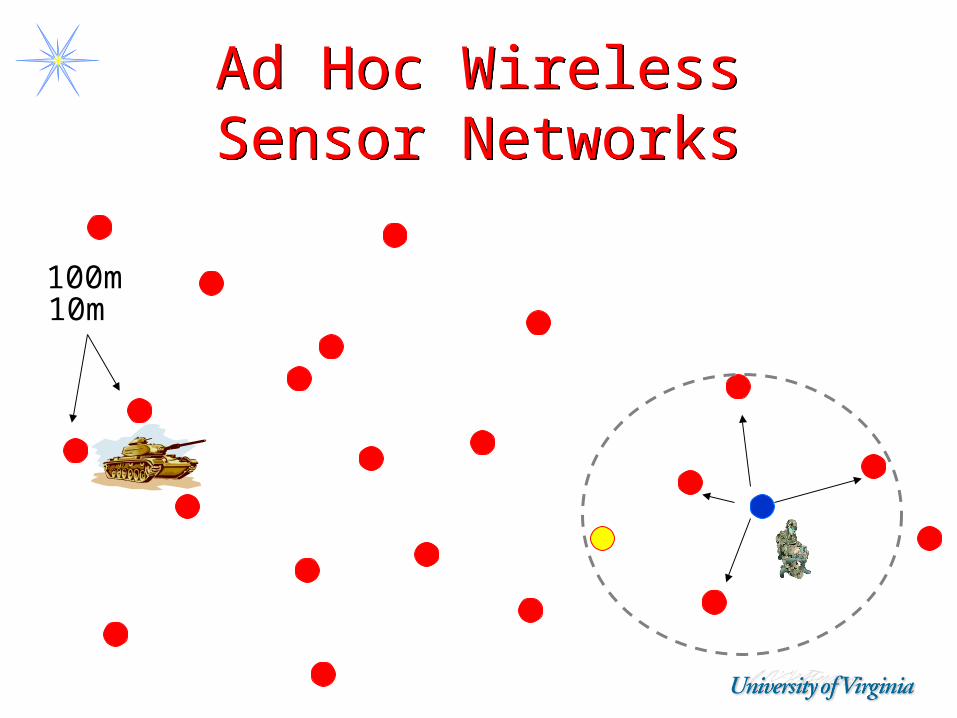
Ad Hoc Wireless Sensor NetworksAd Hoc Wireless Sensor Networks

10m100m

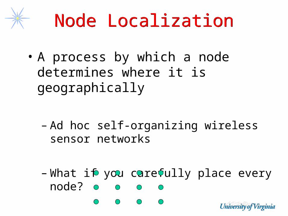
Node LocalizationNode Localization

• A process by which a node determines where it is geographically

– Ad hoc self-organizing wireless sensor networks

– What if you carefully place every node?

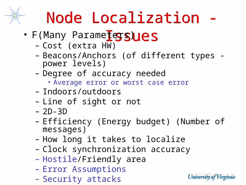
Node Localization - Issues

Node Localization - Issues• F(Many Parameters)

– Cost (extra HW)– Beacons/Anchors (of different types - power

levels)– Degree of accuracy needed

• Average error or worst case error– Indoors/outdoors– Line of sight or not– 2D-3D– Efficiency (Energy budget) (Number of

messages)– How long it takes to localize– Clock synchronization accuracy– Hostile/Friendly area– Error Assumptions – Security attacks

Using LocalizationUsing Localization

• Location of sensor readings to identify where event/target is– Accuracy

• Communication protocols route to area/location– Impact on GF?

• To determine sensing coverage• Location directory service (where is

person A?)

Localization TaxonomyLocalization Taxonomy

• Range Based– Determine distances between nodes

(range)– Then compute location using geometry

• Range Free– No need to determine distances

directly, instead use hop count– Use average distances between hops– Then compute location using geometry

Localization via 3 Distance

Measurements

Localization via 3 Distance

Measurements

X X

X

D1D2

D3

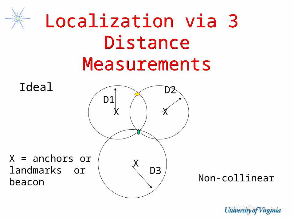
Ideal

X = anchors orlandmarks orbeacon Non-collinear

Localization via N Distance

Measurements

Localization via N Distance

Measurements

X X

X

D1D2

D3

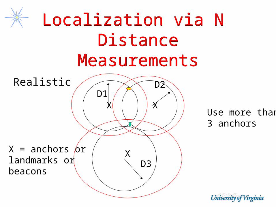
Realistic

X = anchors orlandmarks orbeacons

Use more than3 anchors

Localization Taxonomy

Localization Taxonomy

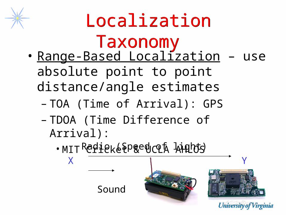
• Range-Based Localization – use absolute point to point distance/angle estimates– TOA (Time of Arrival): GPS– TDOA (Time Difference of Arrival):

•MIT Cricket & UCLA AHLOS

Sound

Radio (Speed of light)

X Y

Range-Based (cont.)Range-Based (cont.)

– AOA (Angle of Arrival):• Aviation System and Rutgers APS

– Signal Strength•Microsoft RADAR and UW SpotOn•Assume signal strength is proportional to

distance– RSSI (received signal strength indicator)

Localization TaxonomyLocalization Taxonomy

• Range-Free Localization – cost is more appropriate for many sensor nodes– USC/ISI Centroid localization – Rutgers DV-Hop Localization– MIT Amorphous Localization – UVA APIT

• Localization that does not rely on information derived from signals. Only Hear/NotHear Distinction (hop count)

TOA - GPSTOA - GPS

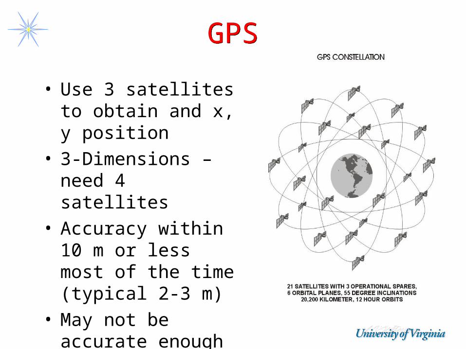
• Constellation of 27 satellites – 24 active and 3 redundant– Clocks must be synchronized (use

signal and clock to compute distance)– Requires line of sight– Billions of dollars of infrastructure

– Each node with GPS is expensive for sensor nodes

– May also be a problem with form factor – makes node too large

GPSGPS

• Use 3 satellites to obtain and x, y position

• 3-Dimensions – need 4 satellites

• Accuracy within 10 m or less most of the time (typical 2-3 m)

• May not be accurate enough

TDOATDOA

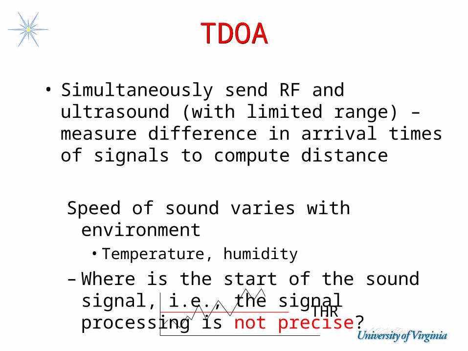
• Simultaneously send RF and ultrasound (with limited range) – measure difference in arrival times of signals to compute distance

Speed of sound varies with environment• Temperature, humidity

– Where is the start of the sound signal, i.e., the signal processing is not precise?

THR

Received Signal Strength Indicator (RSSI)

Received Signal Strength Indicator (RSSI)

• Translate signal strength into distance– Use model/formula to do the conversion– E.g., signal strength drops as inverse

square of distance

• Multi-path fading, background interference, irregular signal propagation render this technique largely unsuitable

Recall - Radio Model Recall - Radio Model

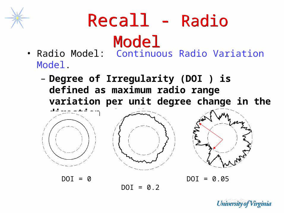
• Radio Model: Continuous Radio Variation Model.– Degree of Irregularity (DOI ) is defined as

maximum radio range variation per unit degree change in the direction of radio propagation

DOI = 0 DOI = 0.05 DOI = 0.2

Range Free: APIT Algorithm

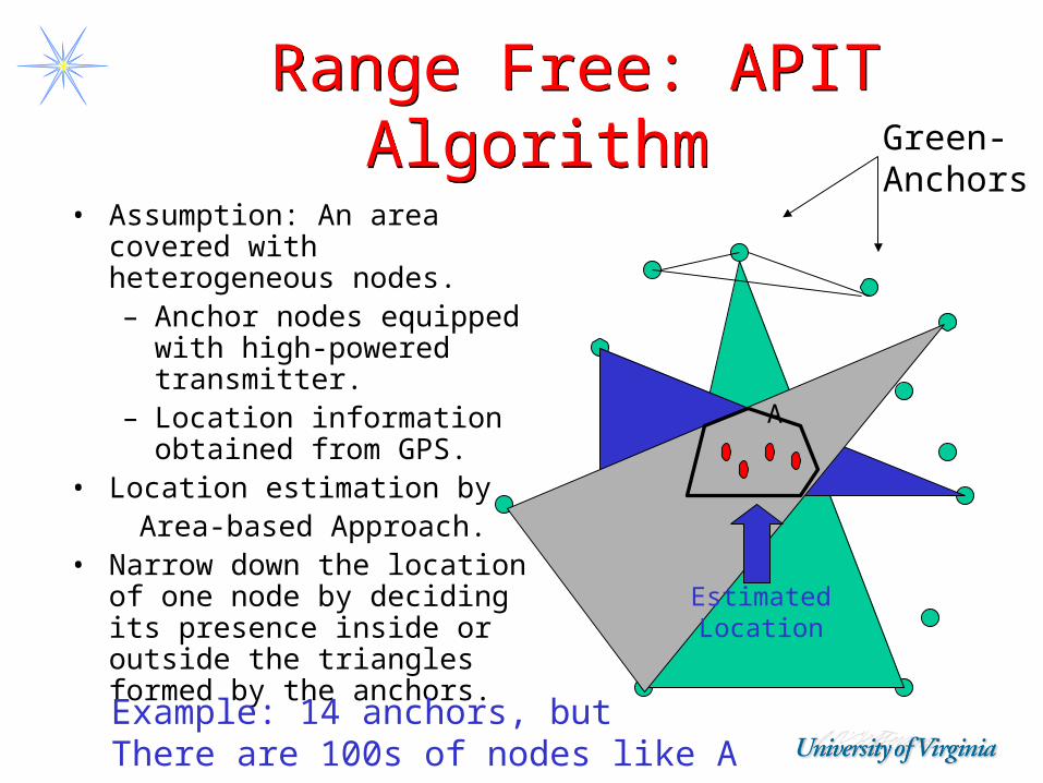
Range Free: APIT Algorithm

• Assumption: An area covered with heterogeneous nodes. – Anchor nodes equipped

with high-powered transmitter.

– Location information obtained from GPS.

• Location estimation by Area-based Approach.• Narrow down the location of

one node by deciding its presence inside or outside the triangles formed by the anchors.

Estimated Location

A

Green-Anchors

Example: 14 anchors, butThere are 100s of nodes like A

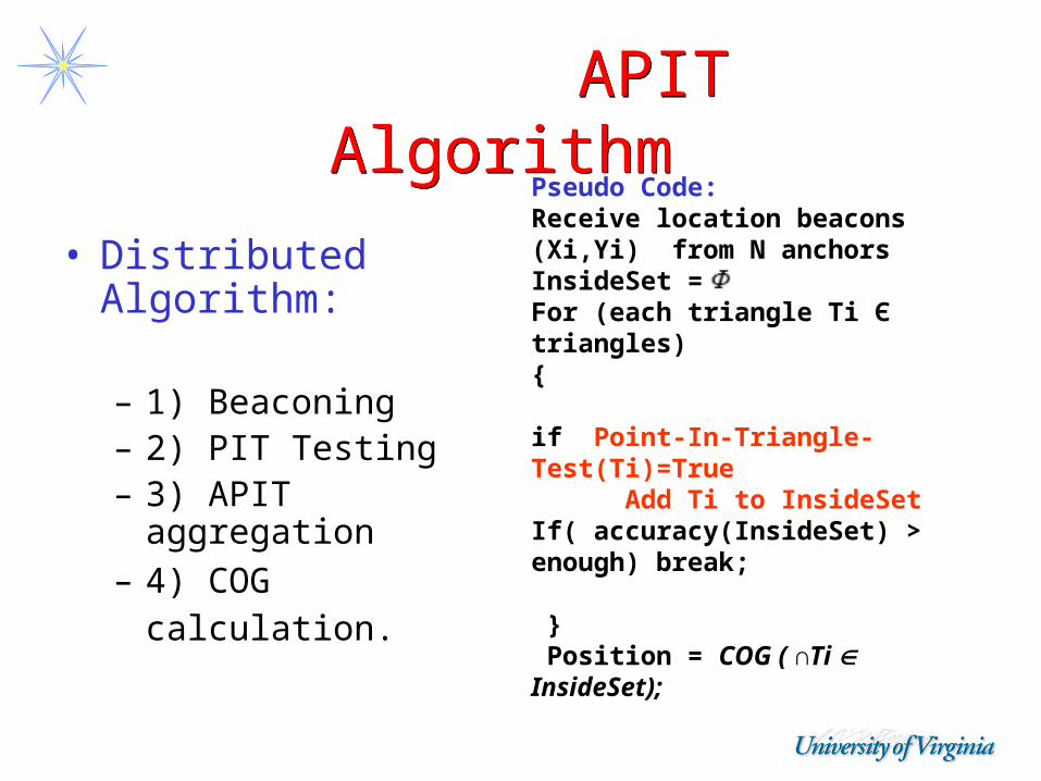
APIT Algorithm APIT Algorithm

• Distributed Algorithm:

– 1) Beaconing– 2) PIT Testing– 3) APIT aggregation

– 4) COG calculation.

Pseudo Code:Receive location beacons (Xi,Yi) from N anchorsInsideSet = For (each triangle Ti Є triangles){

if Point-In-Triangle-Test(Ti)=True Add Ti to InsideSetIf( accuracy(InsideSet) > enough) break;

} Position = COG ( ∩Ti InsideSet);

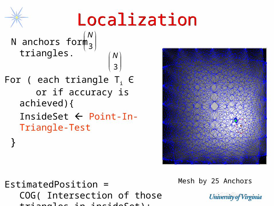
LocalizationLocalization N anchors form triangles.

For ( each triangle Ti Є or if accuracy is achieved){ InsideSet Point-In-Triangle-Test

}

EstimatedPosition = COG( Intersection of those triangles in insideSet);

3

N

Mesh by 25 Anchors

3

N

Point In Triangle Test Point In Triangle Test

• Problem Statement: For three anchors with known positions: A(ax,ay),

B(bx,by), C(cx,cy), determine whether a point M with an unknown position is inside triangle ∆ABC or not.

B(bx,by)C(cx,cy),

A(ax,ay)

M

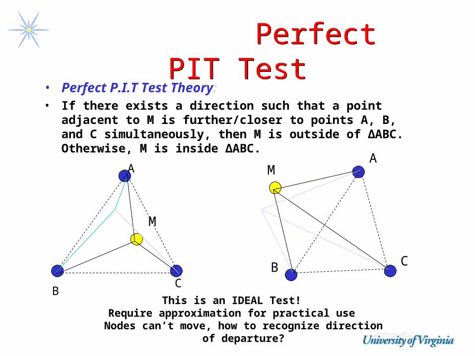
Perfect PIT Test Perfect PIT Test

• Perfect P.I.T Test Theory: • If there exists a direction such that a point adjacent

to M is further/closer to points A, B, and C simultaneously, then M is outside of ∆ABC. Otherwise, M is inside ∆ABC.

A

BC

This is an IDEAL Test!Require approximation for practical use

Nodes can’t move, how to recognize direction of departure?

M

MA

B C

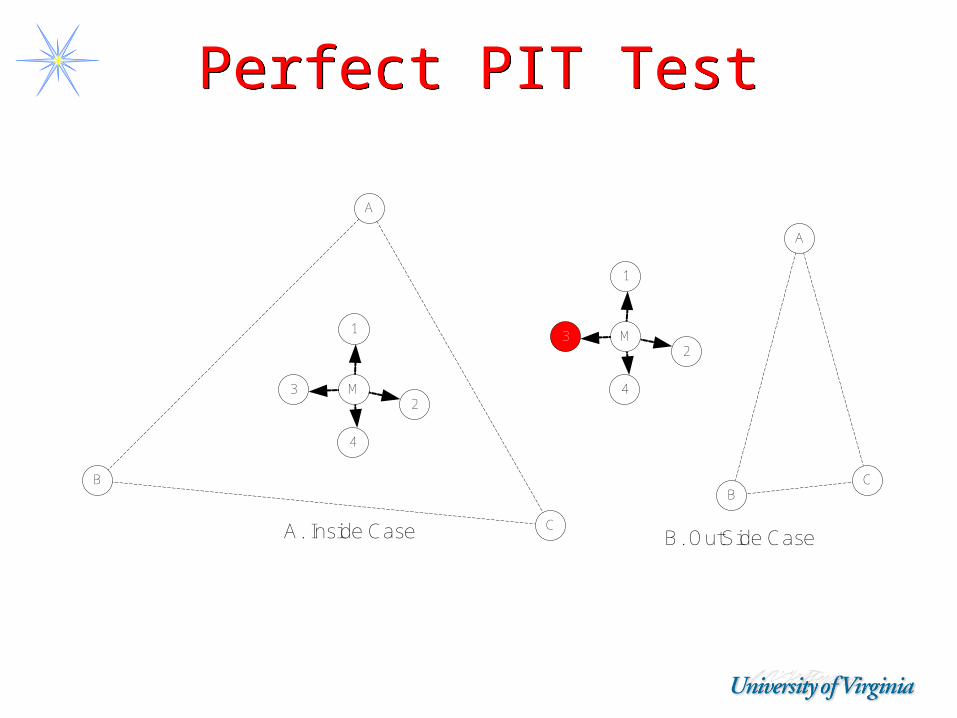
Perfect PIT TestPerfect PIT Test

A

C

1

23

4

M

B

A

CB

A. Inside Case B. OutSide Case

1

23

4

M

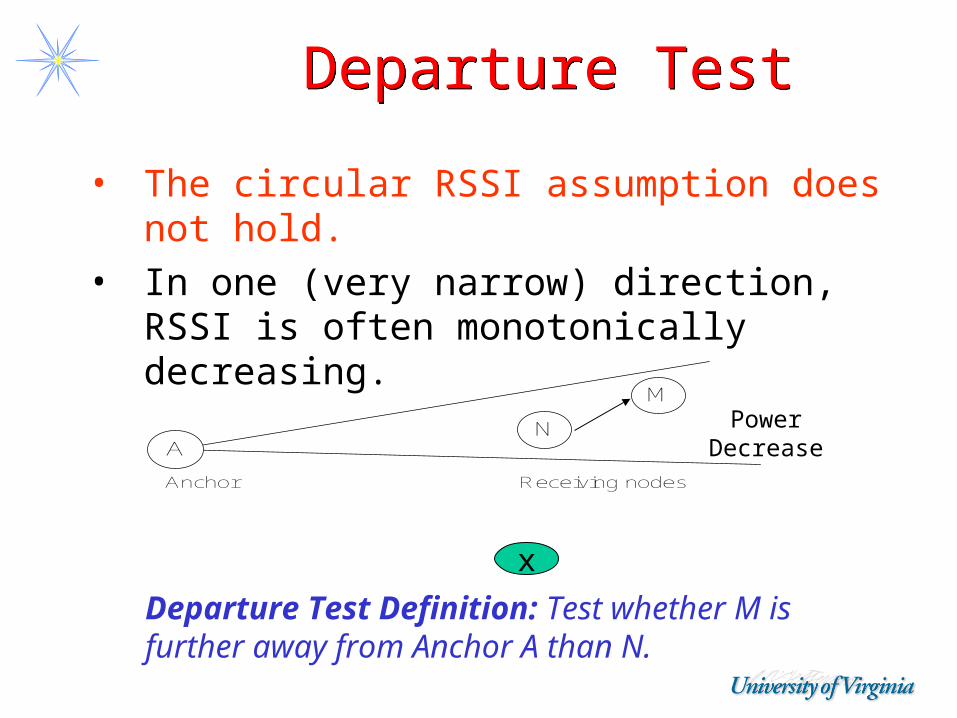
Departure Test Departure Test

• The circular RSSI assumption does not hold.

• In one (very narrow) direction, RSSI is often monotonically decreasing.

M

NA

Anchor Receiving nodes

Power Decrease

Departure Test Definition: Test whether M is further away from Anchor A than N.

x

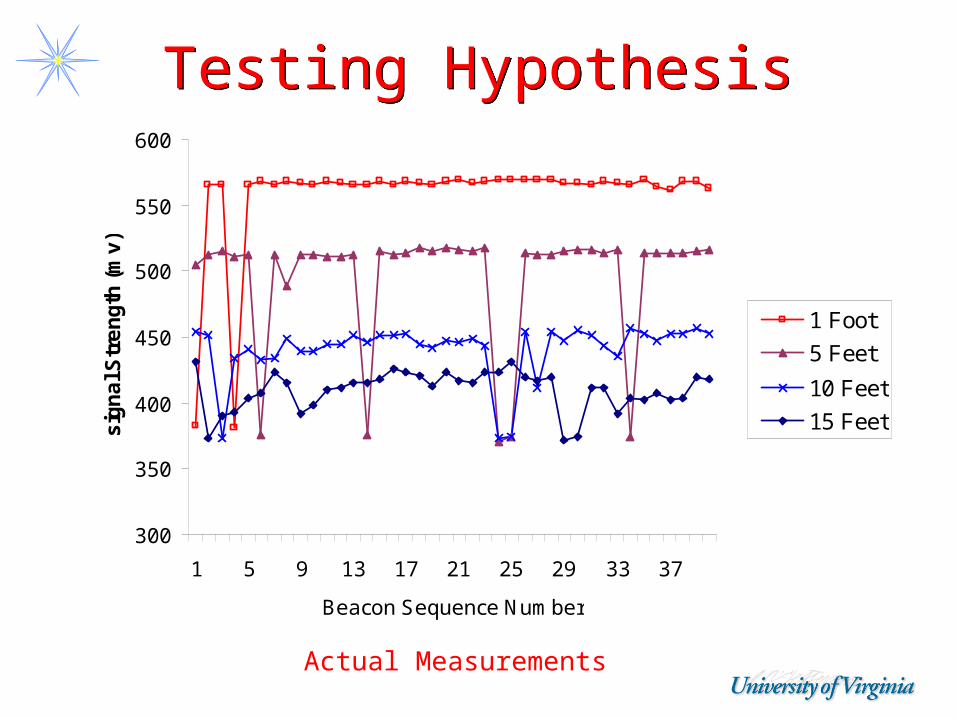
Testing HypothesisTesting Hypothesis

300

350

400

450

500

550

600

1 5 9 13 17 21 25 29 33 37

Beacon Sequence Number

sig

na

l Str

en

gth

(m

v)

1 Foot

5 Feet

10 Feet

15 Feet

Actual Measurements

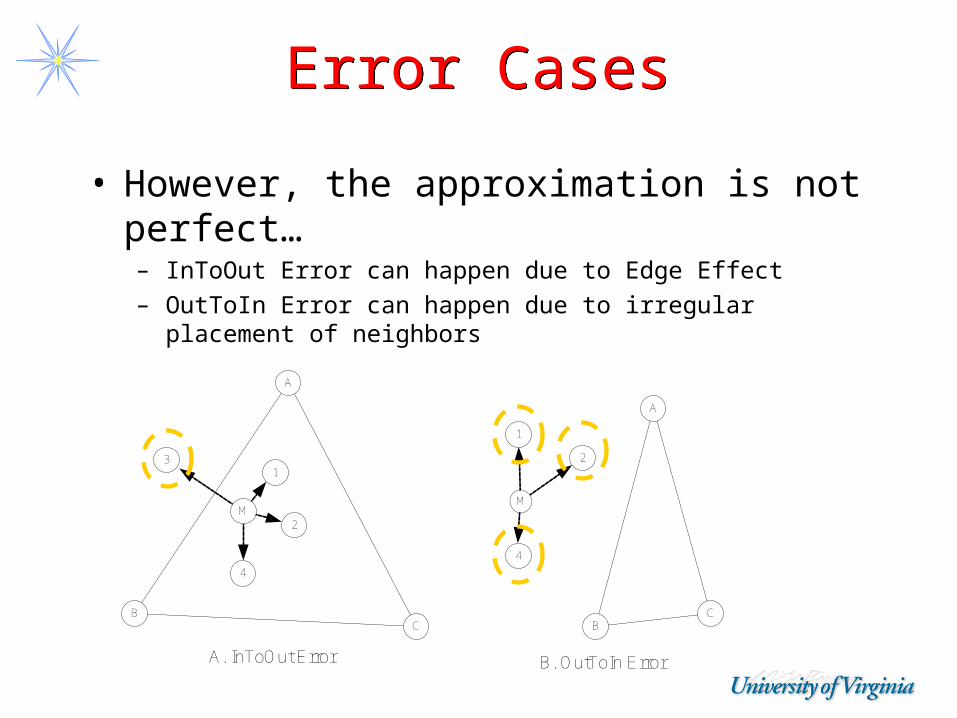
Error CasesError Cases

• However, the approximation is not perfect…– InToOut Error can happen due to Edge Effect– OutToIn Error can happen due to irregular placement of

neighbors

1

2

4

M

A

C

1

2

4

B

A

CB

A. InToOut Error B. OutToIn Error

3

M

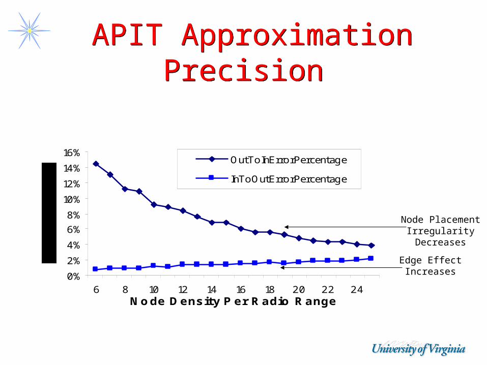
APIT Approximation Precision

APIT Approximation Precision

0%

2%

4%

6%

8%

10%

12%

14%

16%

6 8 10 12 14 16 18 20 22 24Node Density Per Radio Range

OutToInErrorPercentage

InToOutErrorPercentage

Node Placement Irregularity Decreases

Edge Effect Increases

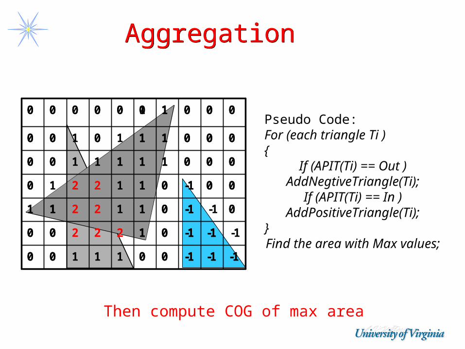
Aggregation Aggregation

-1-1-10011100

-1-1-10122200

0-1-10112211

00-10112210

0001111100

0001110100

0001000000

-1-1-10000

-1-10100

0-1011

00-1010

00011100

00011000

0001100000Pseudo Code:For (each triangle Ti ) {

If (APIT(Ti) == Out ) AddNegtiveTriangle(Ti);

If (APIT(Ti) == In ) AddPositiveTriangle(Ti);

}Find the area with Max

values;

Then compute COG of max area

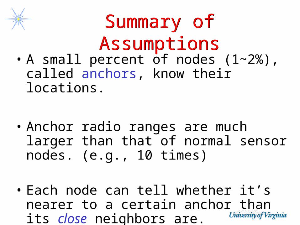
Summary of AssumptionsSummary of Assumptions

• A small percent of nodes (1~2%), called anchors, know their locations.

• Anchor radio ranges are much larger than that of normal sensor nodes. (e.g., 10 times)

• Each node can tell whether it’s nearer to a certain anchor than its close neighbors are.

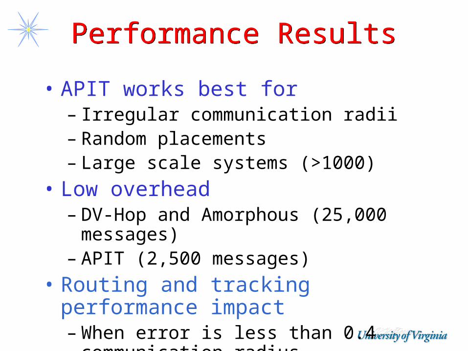
Performance ResultsPerformance Results

• APIT works best for– Irregular communication radii – Random placements– Large scale systems (>1000)

• Low overhead– DV-Hop and Amorphous (25,000

messages)– APIT (2,500 messages)

• Routing and tracking performance impact– When error is less than 0.4

communication radius

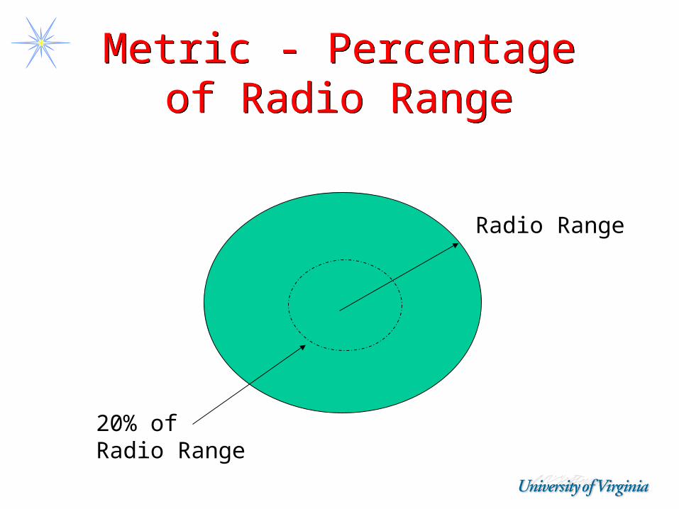
Metric - Percentage of Radio Range

Metric - Percentage of Radio Range

Radio Range

20% ofRadio Range

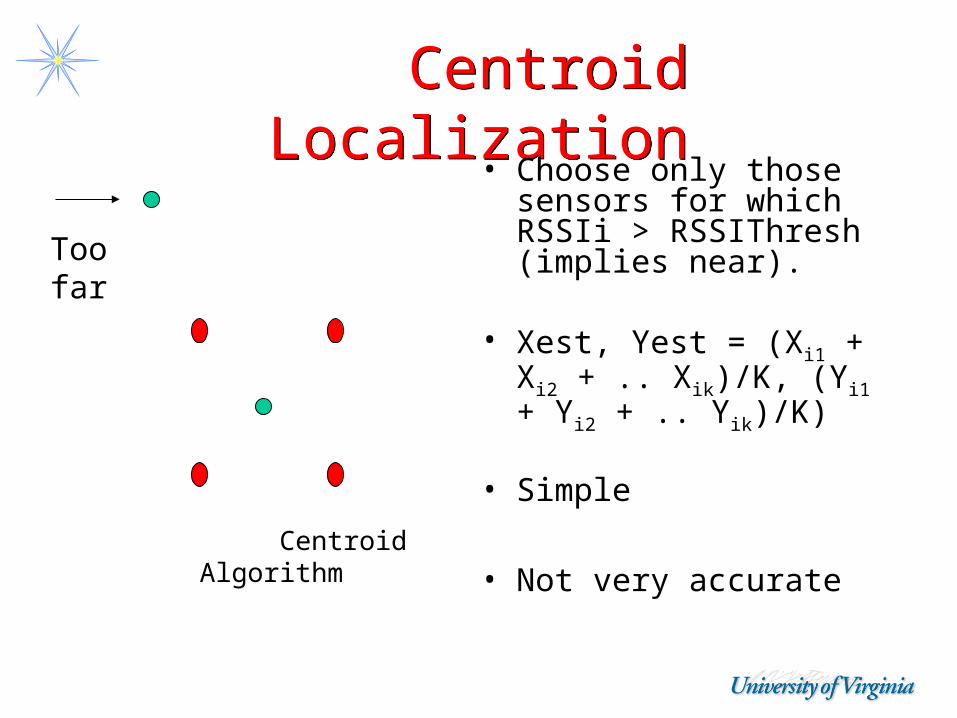
Centroid Localization Centroid Localization

Centroid Algorithm

• Choose only those sensors for which RSSIi > RSSIThresh (implies near).

• Xest, Yest = (Xi1 + Xi2 + .. Xik)/K, (Yi1 + Yi2 + .. Yik)/K)

• Simple

• Not very accurate

Too far

Amorphous Localization Amorphous LocalizationCalculate the

position of the node based on several

given nodes.

Based on hop counts and estimated

distance between nodes.

Compute estimated distance by knowing

size of area and density.

Note: no long range beacons needed like

in APIT.

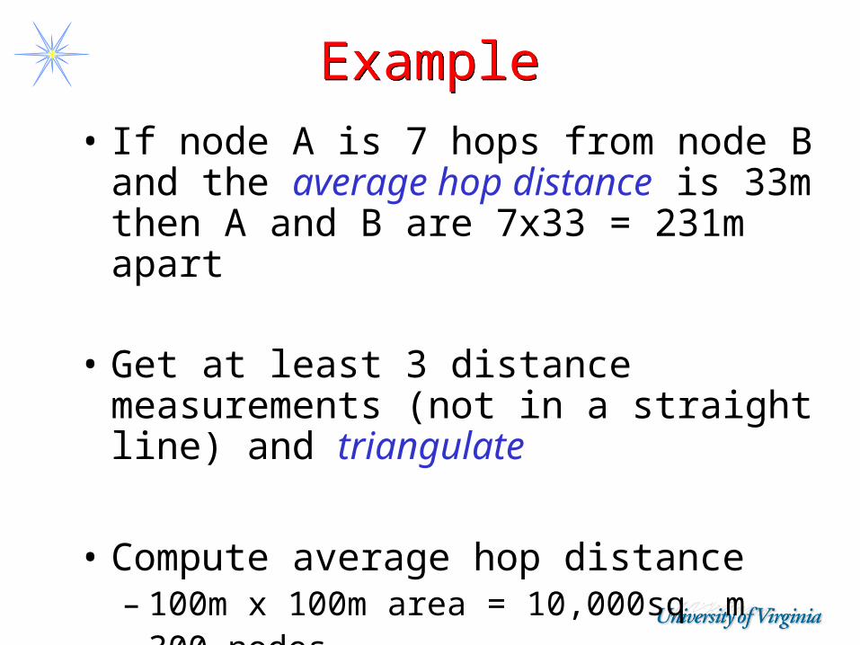
ExampleExample• If node A is 7 hops from node B and

the average hop distance is 33m then A and B are 7x33 = 231m apart

• Get at least 3 distance measurements (not in a straight line) and triangulate

• Compute average hop distance– 100m x 100m area = 10,000sq m– 300 nodes– One node every 33m

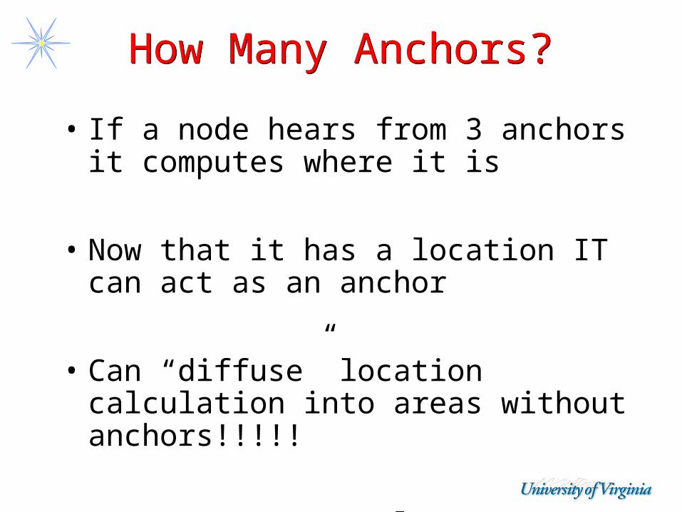
How Many Anchors?How Many Anchors?

• If a node hears from 3 anchors it computes where it is

• Now that it has a location IT can act as an anchor

• Can “diffuse” location calculation into areas without anchors!!!!!

• Errors can accumulate

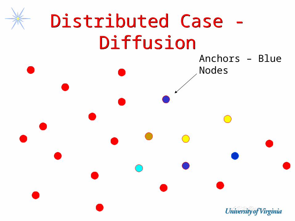
Distributed Case - Diffusion

Distributed Case - Diffusion

Anchors – BlueNodes

Walking GPS – Overview(manual deployment)

Walking GPS – Overview(manual deployment)

• A person or vehicle has a GPS Mote assembly attached to them/it.

• The GPS Mote periodically beacons its location.

• Sensor Motes that receive this beacon infer their location based on the information present in this beacon.

• From the localization perspective, two distinct software components exist. Sensor Mote

Localization

GPS Mote

GPS

GPS Mote

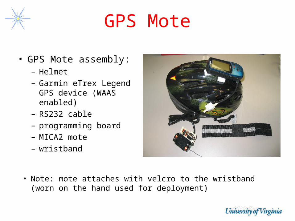
• GPS Mote assembly:– Helmet– Garmin eTrex Legend

GPS device (WAAS enabled)

– RS232 cable– programming board– MICA2 mote– wristband

• Note: mote attaches with velcro to the wristband (worn on the hand used for deployment)

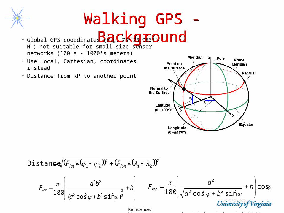
Walking GPS - BackgroundWalking GPS - Background

221

221Distance lonlat FF

h

ba

baFlat

2

32222

22

)sincos(180

cos

sincos180 2222

2

h

ba

aFlon

Reference: http://pasture.ecn.purdue.edu/~abegps/web_ssm/web_GPS.html

• Global GPS coordinates (e.g. 78o 23.9667’ N ) not suitable for small size sensor networks (100's - 1000's meters)

• Use local, Cartesian, coordinates instead• Distance from RP to another point

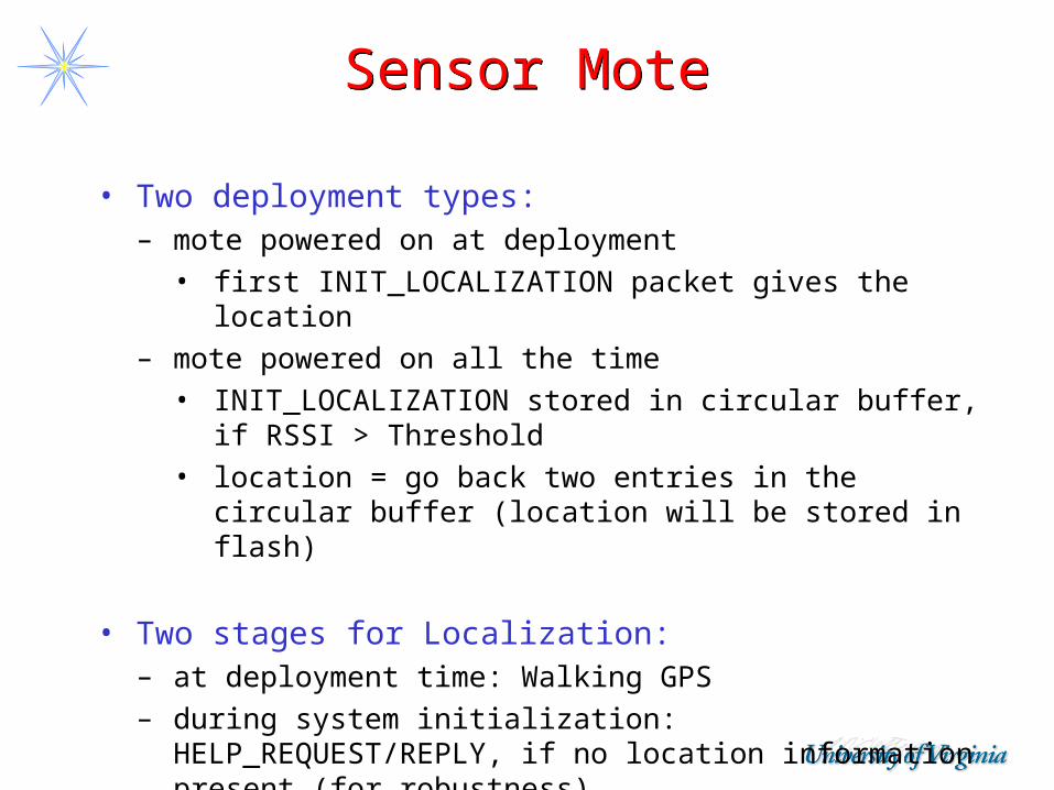
Sensor MoteSensor Mote

• Two deployment types: – mote powered on at deployment

• first INIT_LOCALIZATION packet gives the location– mote powered on all the time

• INIT_LOCALIZATION stored in circular buffer, if RSSI > Threshold

• location = go back two entries in the circular buffer (location will be stored in flash)

• Two stages for Localization:– at deployment time: Walking GPS– during system initialization: HELP_REQUEST/REPLY, if no

location information present (for robustness)

ImplementationImplementation

• Walking GPS device– 17Kbytes of code 595 bytes of data

area

• Field mote– 972 bytes of code– 117 bytes for data area

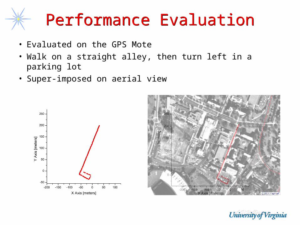
Performance EvaluationPerformance Evaluation• Evaluated on the GPS Mote• Walk on a straight alley, then turn left in a parking lot• Super-imposed on aerial view

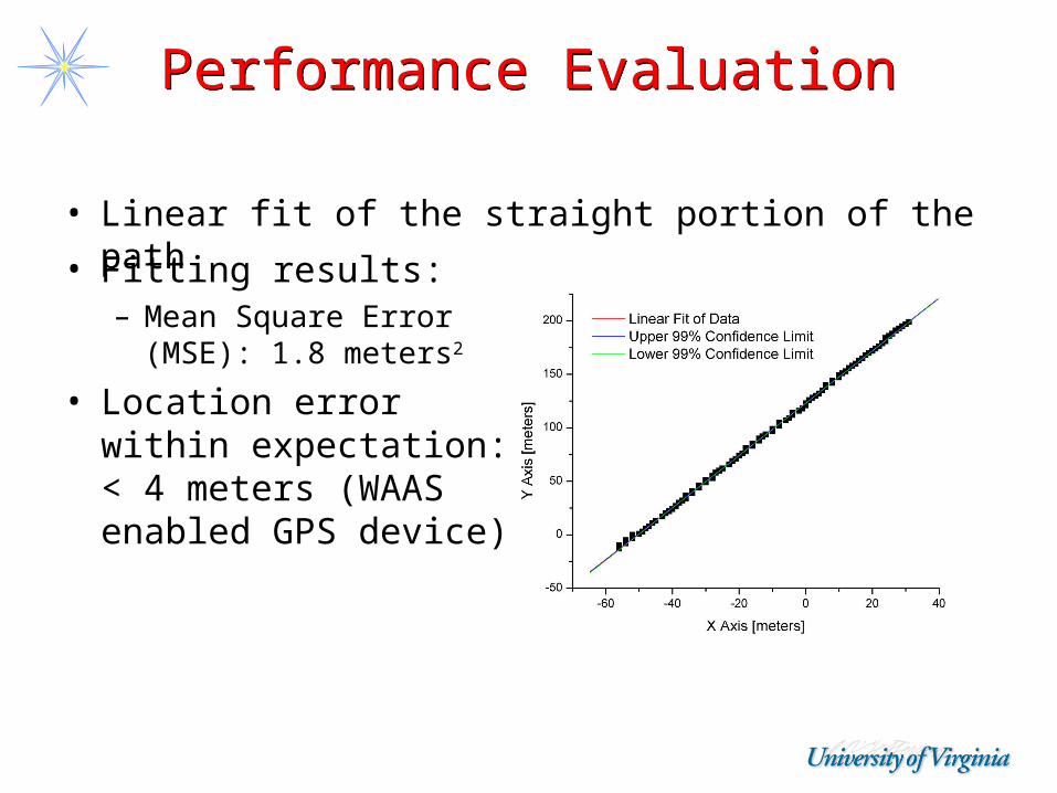
Performance EvaluationPerformance Evaluation

• Linear fit of the straight portion of the path• Fitting results:

– Mean Square Error (MSE): 1.8 meters2

• Location error within expectation: < 4 meters (WAAS enabled GPS device)

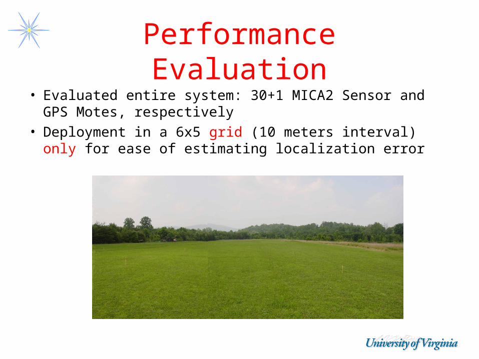
Performance Evaluation

• Evaluated entire system: 30+1 MICA2 Sensor and GPS Motes, respectively

• Deployment in a 6x5 grid (10 meters interval) only for ease of estimating localization error

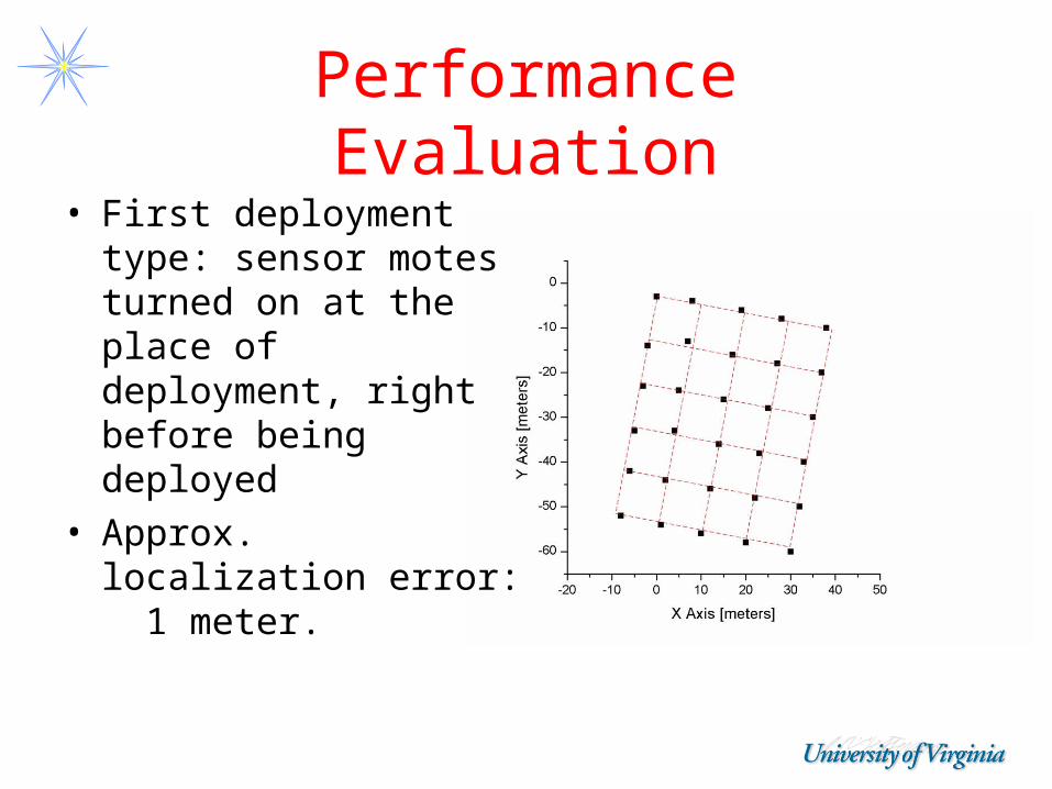
Performance Evaluation

• First deployment type: sensor motes turned on at the place of deployment, right before being deployed

• Approx. localization error: 1 meter.

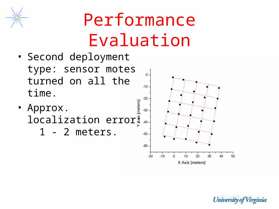
Performance Evaluation

• Second deployment type: sensor motes turned on all the time.

• Approx. localization error: 1 - 2 meters.

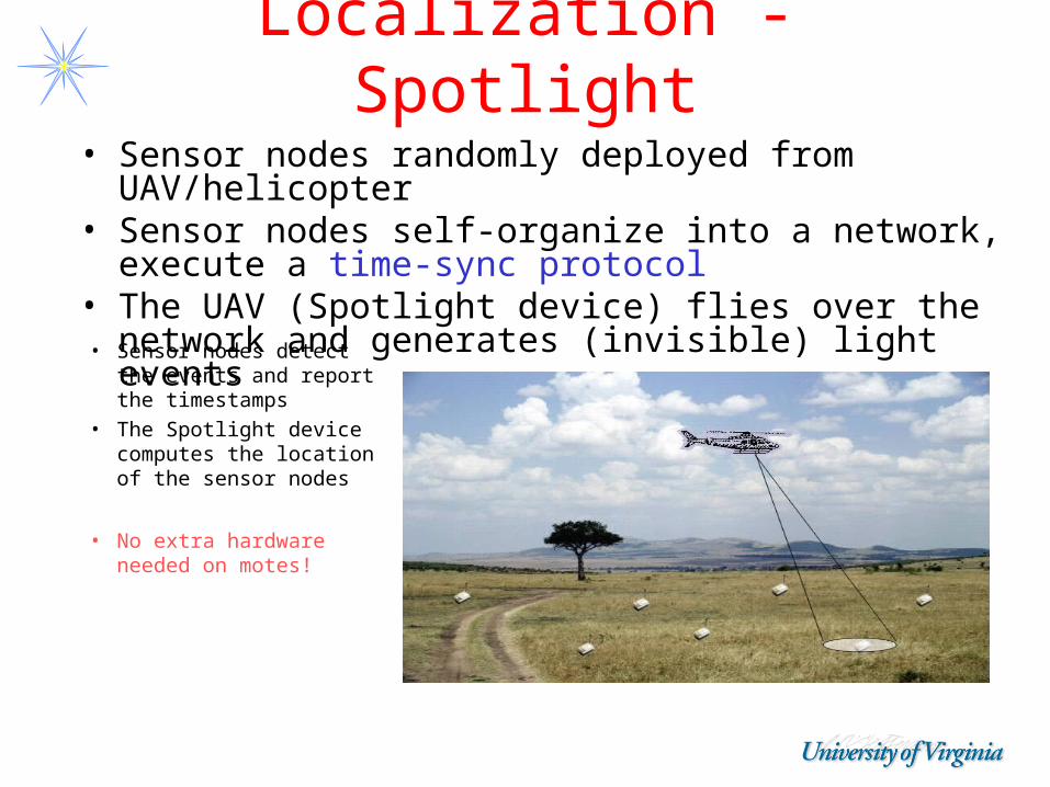
Localization - Spotlight• Sensor nodes randomly deployed from

UAV/helicopter• Sensor nodes self-organize into a network, execute

a time-sync protocol• The UAV (Spotlight device) flies over the network

and generates (invisible) light events• Sensor nodes detect the events and report the timestamps

• The Spotlight device computes the location of the sensor nodes

• No extra hardware needed on motes!

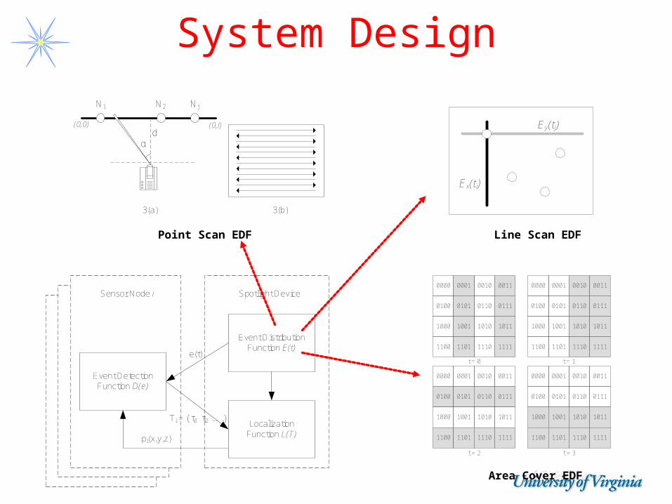
Event DetectionFunction D(e)

Event DistributionFunction E(t)

Localization Function L(T)

e(t)

Ti = { ti1 ti2 ….}

Sensor Node i Spotlight Device

pi(x,y,z)

System Design

(0,0) (0,l)

αd

N2

3(b)3(a)

N1 Nj

Ey(tj)

Ex(ti)

0000 0001 0010 0011

0100 0101 0110 0111

1000 1001 1010 1011

1100 1101 1110 1111

t = 2

0000 0001 0010 0011

0100 0101 0110 0111

1000 1001 1010 1011

1100 1101 1110 1111

t = 0

0000 0001 0010 0011

0100 0101 0110 0111

1000 1001 1010 1011

1100 1101 1110 1111

t = 3

0000 0001 0010 0011

0100 0101 0110 0111

1000 1001 1010 1011

1100 1101 1110 1111

t = 1

Point Scan EDF Line Scan EDF

Area Cover EDF

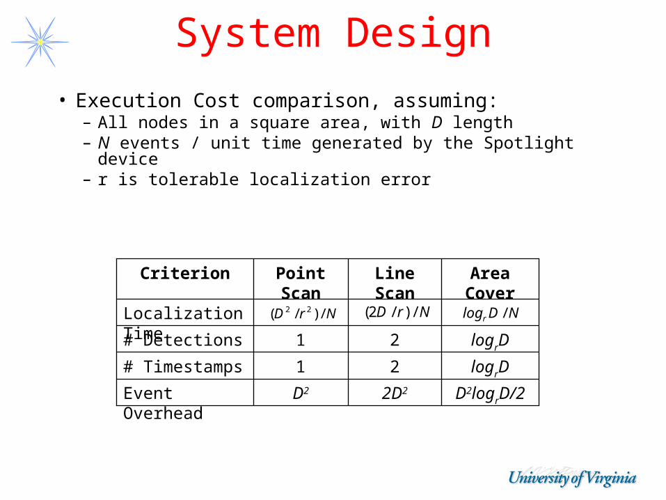
System Design

NrD /)/( 22 NrD /)/2( NDlog r /

D2logrD/22D2D2Event Overhead

logrD21# Timestamps

logrD21# Detections

Localization Time

Area CoverLine ScanPoint ScanCriterion

• Execution Cost comparison, assuming:– All nodes in a square area, with D length– N events / unit time generated by the Spotlight device– r is tolerable localization error

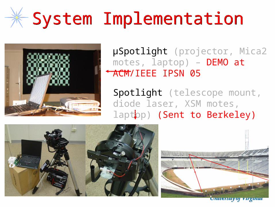
System ImplementationSystem Implementation

μSpotlight (projector, Mica2 motes, laptop) – DEMO at ACM/IEEE IPSN 05

Spotlight (telescope mount, diode laser, XSM motes, laptop) (Sent to Berkeley)

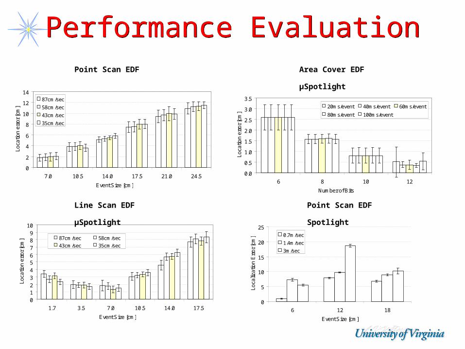
Performance EvaluationPerformance Evaluation

0

5

10

15

20

25

6 12 18

Event Size [cm]

Loc

aliz

atio

n E

rro

r [cm

] 0.7m/sec

1.4m/sec

3m/sec

Point Scan EDF μSpotlight

0

2

4

6

8

10

12

14

7.0 10.5 14.0 17.5 21.0 24.5

Event Size [cm]

Lo

catio

n e

rro

r [c

m]

87cm/sec

58cm/sec

43cm/sec

35cm/sec

0.0

0.5

1.0

1.5

2.0

2.5

3.0

3.5

6 8 10 12

Number of Bits

Lo

catio

n e

rro

r [c

m]

20ms/event 40ms/event 60ms/event

80ms/event 100ms/event

0123456789

10

1.7 3.5 7.0 10.5 14.0 17.5

Event Size [cm]

Lo

catio

n e

rro

r [c

m] 87cm/sec 58cm/sec

43cm/sec 35cm/sec

Area Cover EDF μSpotlight

Line Scan EDF μSpotlight Point Scan EDF Spotlight

Localization - Questions

Localization - Questions

• Stealthy– No manual deployment– Minimize packets

• Minimum cost, time, energy• Handling errors and outliers• Node, Target and Location Directory

Services• Security

SummarySummary

• Critical issue for WSN– Accurate, Robust and Secure– Impacts MAC, Routing, ,,,

• If fixed infrastructure – many solutions work

• Normally executed once at system init time– What if mobile system– What if nodes get moved

SummarySummary

• Range Based– Expensive for large systems

• Range-free– Too many based on general signal

strength– Variations in assumptions about types

of beacons, etc.– APIT improvement over Centroid,

Amorphous, DV-Hop– Walking GPS – practical

SummarySummary

• Fn(Many Parameters)– HW, beacons of different types, degree

of accuracy needed, indoors/outdoors, 2D-3D, energy budget, how well clocks can be synchronized, …)

• More work to be done– Exploit deployment information (e.g.,

you know that you are trying to deploy the nodes in a grid)

– Robust and Secure (worst case error not average; attack resistant)