Winner’s Curse and the Competitive E ect - Economics 2010 Winner’s Curse and the Competitive E...
28
Winner’s Curse and the Competitive Effect: Measuring Competition in the Viatical Settlement Market Peter Tu [email protected] Department of Economics Stanford University Stanford, CA 94305 Advisor: Jay Bhattacharya May 10, 2010 Abstract This paper attempts to develop a methodology for measuring competition in markets where the object for sale has a common but unknown monetary value. We do this by conceptualizing transactions in the viatical settlement market as first-price, common value auctions and deriving a parametric model for equilibrium bid functions. Within this model, we then estimate parameters and make observations about bidder behavior. Our analysis finds on average, fewer than five bidders compete for viatical contracts. We believe this is strong evidence of market power. Finally, by simulating comparative statics on the distribution of number of bidders, we conclude that at our estimated levels of competition, any evidence of winner’s curse was completely dominated by the competitive effect. Keywords: winner’s curse, viatical settlement, competitive effect, common value auction, life insurance This thesis would not have made it to its current state if not for the direction, patience and amazing encouragement from Professor Jay Bhattacharya. I also express endless gratitude to Professor Han Hong; his vast knowledge has been inspiring. Lastly, thanks go to all my friends who have been so incredibly supportive. 1
Transcript of Winner’s Curse and the Competitive E ect - Economics 2010 Winner’s Curse and the Competitive E...
Winner’s Curse and the Competitive Effect:Measuring Competition in the Viatical Settlement Market
Peter [email protected]
Department of EconomicsStanford UniversityStanford, CA 94305
Advisor: Jay Bhattacharya
May 10, 2010
Abstract
This paper attempts to develop a methodology for measuring competition in marketswhere the object for sale has a common but unknown monetary value. We do this byconceptualizing transactions in the viatical settlement market as first-price, commonvalue auctions and deriving a parametric model for equilibrium bid functions. Withinthis model, we then estimate parameters and make observations about bidder behavior.Our analysis finds on average, fewer than five bidders compete for viatical contracts.We believe this is strong evidence of market power. Finally, by simulating comparativestatics on the distribution of number of bidders, we conclude that at our estimatedlevels of competition, any evidence of winner’s curse was completely dominated by thecompetitive effect.
Keywords: winner’s curse, viatical settlement, competitive effect, common value auction,life insurance
This thesis would not have made it to its current state if not for the direction, patience and amazingencouragement from Professor Jay Bhattacharya. I also express endless gratitude to Professor HanHong; his vast knowledge has been inspiring. Lastly, thanks go to all my friends who have been soincredibly supportive.
1
Tu 2010 Winner’s Curse and the Competitive Effect
Contents
1 Introduction 3
2 Bidding for Viatical Settlements 4
3 Assumptions for Empirical Analysis 103.1 The Distribution of Contract Values . . . . . . . . . . . . . . . . . . . . . . . . . . . 103.2 The Distribution of Signals of Contract Value . . . . . . . . . . . . . . . . . . . . . . 113.3 The Distribution of the Number of Bidding Firms . . . . . . . . . . . . . . . . . . . 12
4 Data 13
5 Empirical Strategy 16
6 Results 186.1 Effect of Increased Competition . . . . . . . . . . . . . . . . . . . . . . . . . . . . . . 20
7 Conclusion 23
8 Appendix: Calculation of Standard Errors 24
2

Tu 2010 Winner’s Curse and the Competitive Effect
1 Introduction
Fundamental to economics is the core postulate that increased competition improves social welfare,
and that perfect competition is welfare maximizing. Hence, measuring the level of competition is
essential for evaluating the functioning of any market. We attempt to add to literature on this
topic by conceptualizing a market as a first-price auction. In this framing, the final auction price
is determined by the number of bidders and the ability of these bidders to reliably judge the value
of the auctioned item. The number of bidders serves as our measure of competition, and using an
auction model, we can measure the impact of competition and information on market efficiency.
We conduct this analysis on data between 1995-2001 from the secondary life insurance market,
where transactions known as viatical settlements allowed life insurance holders to trade their future
death benefits for immediate payouts. Participants in this market were typically those who had
previously purchased a life insurance policy but were recently diagnosed with a terminal illness. The
insured individual can then agree to gain a lumpsum cash benefit now in exchange for listing the
third-party purchaser as the policy’s sole beneficiary. This purchaser, a viatical firm, then receives
the full face value upon the policyseller’s (i.e. viaticator’s) death. Though the eventual value to
the viatical firm is constant at the policy face value, the firm cannot collect until after the seller’s
death, so it shoulders risks that the insured outlives the predicted life expectancy or that the death
occurs in such a way that voids the policy. The insured individual’s predicted life expectancy and
judgment of these risks determine the viatical settlement amount that the policy seller receives,
and this amount is inversely related to life expectancy and the level of uncertainty.
Even when purchasers price against these risks, the sale of a life insurance policy can be pareto-
improving. Sellers benefit from the heightened liquidity, which can finance vital end-of-life medical
care or consumption. Viatical settlement payouts also generally greatly exceed the policies’ cash
surrender values, because the cash surrender value calculation neglects to adjust for the policy-
holder’s alterred health status. Hence, the viatical insurance market can be a source of much
needed equity for the terminally ill. Despite this potential benefit, the viatical market faces its
criticisms, ranging from the benign ”macabre” (Goldstein 2007) to the more condemning ”ghoul-
ish, perverse and vampire” (Quinn 2008). Parts of this backlash stem from moral discomfort about
the business of death speculation. Others worry about the moral hazards present when the new
life insurance policy owner post-transaction suddenly has economic interest in an early death of
the insured. Fears of abuse in this market are also accentuated by the possibly acute vulnerability
of the policy seller. Could the terminally ill be exploited into giving up their policies for ”below
market” rates?
This conflict has drawn scrutiny into the ethics of viatical settlements and also spurred attempts
to regulate the market (Trinkaus and Giacalone 2002; Quinn 2008). Gloria Grening-Wolk fears that
viatical firms exploit consumers by exercising market power, and four-time Presidential candidate
Ralph Nader too has spoken out for regulation (Grening Wolk 1997). We attempt to evaluate these
claims of imperfect competition by comparing settlement values to the actuarially fair prices.
Several other factors make the secondary insurance market between 1995-2001 worthy of study.
3
Tu 2010 Winner’s Curse and the Competitive Effect
First, the market has undergone tremendous change in a small number of years. Though a Supreme
Court decision upheld their legality in 1911 (Quinn 2008), viatical transactions remained very rare
until the surge in HIV/AIDS in the early 1990s. So the market was still fairly new in 1995. We
also hypothesize that the market was deeply altered by the arrival of efficacious treaments for
HIV in 1996. The adoption of Highly Active Anti-Retrovireal Therapy (HAART) almost overnight
removed HIV/AIDS as an immediate death sentence. Because our data spans the adoption of this
new treatment, we can assess the impact of HAART on calculations of mortality risk as well as its
effect on market competition.
Lastly, though our data supports other reports that the popularity of viatical settlements has
fallen dramatically since its peak in the mid-1990s (Belth 2000), the market seems not to have
vanished but transitioned from the terminally ill to the elderly. Those transactions between policy
purchasers and the elderly known as life settlements reached $3.4 billion in 2005 (LISA 2007) and
an estimated $12.2 billion in 2007 (Tergesen 2008). As end of life care becomes more expensive,
the importance of this secondary insurance market will only grow. Hence, learnings gained from
our investigation into the 1995-2001 viatical settlement market may be insightful for current policy
questions about this burgeoning market as well.
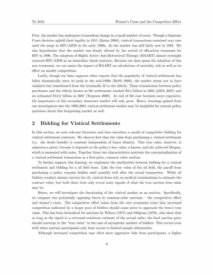
2 Bidding for Viatical Settlements
In this section, we note relevant literature and then introduce a model of competitive bidding for
viatical settlement contracts. We observe first that the value from purchasing a viatical settlement
(i.e. the death benefit) is constant independent of buyer identity. This true value, however, is
unknown a priori, because it depends on the policy’s face value, a known, and the achieved lifespan,
which is measured with noise. Together these two characteristics motivate the conceptualization of
a viatical settlement transaction as a first-price, common value auction.
To further support this framing, we emphasize the similiarities between bidding for a viatical
settlement and bidding for a oil field lease. Like the true value of the oil field, the payoff from
purchasing a policy remains hidden until possibly well after the actual transaction. While oil
bidders conduct seismic surveys for oil, viatical firms rely on medical examinations to estimate the
contract value, but both these tests only reveal noisy signals of what the true auction item value
may be.
Hence, we will investigate the functioning of the viatical market as an auction. Specifically,
we compare two potentially opposing forces in common-value auctions – the competitive effect
and winner’s curse. The competitive effect arises from the core economics tenet that increased
competition indicated by a larger pool of bidders should cause price to approach the item’s true
value. This has been formalized for auctions by Wilson (1977) and Milgrom (1979), who show that
as long as the signal is a extremal-consistent estimate of the actual value, the final auction price
should converge to the “true value” in the case of asymptotic number of bidders. This occurs even
with when auction participants only have access to limited sample information.
Although increased competition may elicit more aggressive bids from participants, a higher
4

Tu 2010 Winner’s Curse and the Competitive Effect
number of bidders also raises the spectre of winner’s curse, which occurs when auction winners
receive a negative profit because their signal overestimated the contract’s true value. This fear
of having an overly-optimistic value estimate encourages more cautious bidding behavior, and the
more bidders the more caution. This has led Bulow and Kemperer (2002) to argue that in some
scenarios, restricting entry into the auction may actually increase prices, because bidders may shade
their bids less. Literature has agreed that that auction participants are aware of the winner’s curse,
and in equilibrium, at least the sophisticated bidders do incorporate it into their bidding strategies
(Harrison and List 2008). For example, Hendricks, Pinkse and Porter (2003) found evidence of
winner’s curse internalized into bidding behavior for wildcat oil leases on the Outer Continental
Shelf from 1954 to 1970. We similarly conjecture that firms acting in the viatical settlement market
are sophiscated enough to protect against winner’s curse in their equilibrium strategies.
Thus, bidder behavior in common value auctions reacts mainly to these two effects – higher
competition and winner’s curse. Paarsch (1992) argues that bids and therefore, prices should
initially rise with increased competition as participants reduce their profit padding to increase
the probability of winning. However, beyond a certain point, the adverse selection impact of
winner’s curse eclipses the competitive effect as potential purchasers increasingly shade their bids
to avoid negative profits. The critical point of balancing these two effects remains an open question
depending on market attributes (Armantier 2002), though Kagel and Levin (2002) in their survey of
experimental common value auctions, claim that at least five bidders are necessary before winner’s
curse arises.
Also crucial to the functioning of common value auctions is the reliability of bidders’ signals of
the auctioned item’s true value. Poor estimates raise the risk associated with participating in the
auction and so may distort bids downward. An auction might also collapse if buyers and sellers
do not share the same information set. Specifically, if viaticators know their own mortality risks
better than the firms, then Akerlof’s market for lemons problem of adverse selection might arise
(1970). The market would also be impacted if policy sellers have biased judgments about their
own mortality risk depending on their perceptions of death. But Cawley and Philipson (1999)
develop evidence that in life insurance markets, firms and consumers make decisions from the same
information set. Similarly, Bhattacharya and Snood (2001) argue that the the viatical settlement
market better matches the full-information model than adverse selection ones.
Literature on parametrically estimating common auction models has been more limited. Most
of the early work including Rothkopf (1969), Smiley (1979), Thiel (1988) and Levin and Smith
(1991) have relied on bidding models that produce closed-form solutions, which enable estimation
through non-linear least squares or maximum likelihood (Paarsch 1994). The model we propose
does not lend itself as easily to a closed form, so we opt instead to emulate the simulated non-linear
least squares strategy taken by Hong and Shum (2002).
Lastly, before we develop our model, we describe an important difference between our con-
ceptualization and the more canonical auction model. For a viatical settlement transaction, the
policy seller approaches viatical firms to request offers. This is different from the case of an oil
field when interested bidders take the initiative to conduct seismic surveys. So the number of offers
5

Tu 2010 Winner’s Curse and the Competitive Effect
for a viatical settlement may be better modeled as a sequential search for an acceptably high bid.
Additionally, auction entry may be endogenous to the viaticator’s search costs and health. While
this presents a possible extension to our analysis, we will instead argue that the number of bidding
firms can be well-modeled by a probability distribution known to all viatical firms.
We develop our model of viatical settlement auctions with the following notation:
Let N be the number of firms that the seller chooses to contact.
Let i be an index over the N , and let Πi represent firm i’s profits.
Let bi be firm i’s bid, so b = (b1, ...bN ) denotes a vector of firm bids.
Let r be the fixed interest rate.
Let v be the true value from winning the auction. In the viatical settlements market, this
value depends upon the life expectancy of the seller (longer life expectancy implies a smaller
v) and upon the interest rate (increases in r also imply a smaller v). G(v) represents the
cumulative distribution function of v over the population of viaticators. For a policy with
face value C, g(v) has support on (0, C].
When a seller approaches a firm, the potential bidder receives a noisy signal xi of the true
value of the viatical settlement. Fv(xi) = F (xi|v) is the cumulative distribution of xi given
the viatical settlement’s true value. Similarly, fv(xi) also has support over [0, C].
When the firm bids on a contract, it does not know the number of other firms that it competes
against. But the firm does the distribution of N , which we denote by pn = P [N = n].
Let Bi denote the event that bi is the winning bid, Bi = bi > bj∀j 6= i. Analogously, Xi
represents the event that firm i’s signal dominates all others, Xi = xi;xi > xj∀j 6= i.
To derive the equilibrium bidding function, we modify a strategy well-documented in literature
(Paarsch and Hong 2006, p.34). We assume a market of risk-neutral firms striving to maximize
expected profits. Firm i’s expected profit if it makes a bid of bi is the probability that it wins the
auction times the expected return it earns after paying that bid.
E[Πi|xi, bi] = P [Bi|xi] (E[v|xi, Bi]− bi) (1)
=
∞∑n=1
pnP [Bi|N = n] (E [v|xi, Bi, N = n]− bi)
In this model, before their reading of the seller’s health, xi, all firms are exactly alike. This
observation motivates our assumption that the firm’s bidding strategies are symmetric. Moreover,
we model that separate estimates of the viaticator’s health are independent since bidders each
conduct their own medical examinations independently.
To maximize E [Π|xi, bi], firm chooses bi to satisfy the first order condition:
6

Tu 2010 Winner’s Curse and the Competitive Effect
∂E[Π|bi]∂bi
=
∞∑n=1
pn
(∂P [Bi|n]
∂bi(E [v|Bi, n]− bi)− P [Bi|xi, n]
)= 0 (2)
Equations (2) says firms maximize expected profits by equating the marginal increase in ex-
pected revenue due to the higher probability of winning with the marginal cost of paying out that
higher bid.
Rearranging the first order condition (2) yields:
bi =
∞∑n=1
pn
(∂P [Bi|n]
∂biE [v|Bi, n]− P [Bi|n]
)∞∑
n=1
pn∂P [Bi|n]
∂bi
(3)
Let β be firm i’s bidding strategy, so bi = β(xi), and we claim that symmetric firms share
the same strategy. The bidding function, β is monotonically increasing in xi, so we can write
xi = β−1(bi). Along with this monotonicity property, firm symmetry permits a simple way to
calculate the probability that a bid of bi will win in an auction with n participants.
P [Bi|n] =
∞∫0
g (v)[Fv
(β−1 (Bi)
)]n−1dv (4)
Differentiating this equation with respect to bi yields,
∂P [Bi|n]
∂bi=
∞∫0
g (v) (n− 1)[Fv
(β−1 (bi)
)]n−2 fv (β−1 (bi))
β′ (bi)dv (5)
Our theoretical goal is to obtain an an analytic expression for β(x) in equilibrium. The next
steps manipulate our original first order condition to derive such an expression. First, we distribute
equation (3) into two terms:
bi = β (xi) =
∞∑n=1
pn∂P [Bi|n]
∂biE [v|Bi, n]
∞∑n=1
pn∂P [Bi|n]
∂bi
−
∞∑n=1
pnP [Bi|n]
∞∑n=1
pn∂P [Bi|n]
∂bi
(6)
Next, we plug equations (4) and (5) into equation (6).
7

Tu 2010 Winner’s Curse and the Competitive Effect
β (xi) =
∞∑n=1
pnE [v|Bi, n]
∫ ∞0
g (v) (n− 1) [Fv (xi)]n−2 fv (xi)
β′ (xi)dv
∞∑n=1
pn
∫ ∞0
g (v) (n− 1) [Fv (xi)]n−2 fv (xi)
β′ (xi)dv
−
∞∑n=1
pn
∫ ∞0
g (v) [Fv (xi)]n−1
dv
∞∑n=1
pn
∫ ∞0
g (v) (n− 1) [Fv (xi)]n−2 fv (xi)
β′ (xi)dv
(7)
Since β′(x) does not depend on n, we pull these terms out of the summations in equation (7).
Cancelling terms then yields:
β (xi) =
∞∑n=1
pnE [v|Bi, n]
∫ ∞0
g (v) (n− 1) [Fv (xi)]n−2
fv (xi) dv
∞∑n=1
pn
∫ ∞0
g (v) (n− 1) [Fv (xi)]n−2
fv (xi) dv
−
∞∑n=1
pn
∫ ∞0
g (v) [Fv (xi)]n−1
dv
∞∑n=1
pn
∫ ∞0
g (v) (n− 1) [Fv (xi)]n−2
fv (xi) dv
β′ (xi)
(8)
Next, we solve (8) for β′(x) as a function of β(x). This gives us a first order linear differential
equation of β(x) in standard form:
β′ (xi) =
∞∑n=1
pnE [v|Bi, n]
∫ ∞0
g (v) (n− 1) [Fv (xi)]n−2
fv (xi) dv
∞∑n=1
pn
∫ ∞0
g (v) [Fv (xi)]n−1
dv
−
∞∑n=1
pn
∫ ∞0
g (v) (n− 1) [Fv (xi)]n−2
fv (xi) dv
∞∑n=1
pn
∫ ∞0
g (v) [Fv (xi)]n−1
dv
β (x)
(9)
The theory of ordinary linear differential equations then gives us that for an equation of the
form β′(x) = Q(x)−R(x)β(x), the solution for β(x) is:
β (x) = exp
(−∫ x
R (u) du
)[∫ x
Q (u) exp
(∫ u
R (y) dy
)du+ c
], (10)
where c is an arbitrary real number.
Clearly, the terms in equation (9) line up directly with equation (10). Hence,
8

Tu 2010 Winner’s Curse and the Competitive Effect
∫ x
R (u) du =
∫ x∑∞
n=1 pn∫∞0g(v)(n− 1) [Fv(u)]
n−2fv(u)dv
∞∑n=1
∫ ∞0
g(v) [Fv(u)]n−1
dv
du
= ln
[ ∞∑n=1
pn
∫ ∞0
g(v) [Fv(u)]n−1
dv
](11)
This gives:
exp
(∫ x
R (u)du
)=
∞∑n=1
pn
∫ ∞0
g (v) [Fv (xi)]n−1
dv (12)
Similarly, ∫ x
Q (u) exp
(∫ u
R (y)dy
)du =∫ x
( ∞∑n=1
pnE [v|Bi, n]
∫ ∞0
g (v) (n− 1) [Fv (u)]n−2
fv (u) dv
)du (13)
Plugging equations (12) and (13) into equation (10) gives our final solution for β(x):
β (x) =
∫ x
0
( ∞∑n=1
pnE [v|Bi, n]
∫ ∞0
g (v) (n− 1) [Fv (u)]n−2 fv (u) dv
)du
∞∑n=1
pn
∫ ∞0
g (v) [Fv (x)]n−1 dv
(14)
The integration constant must equal zero, since in equilibrium, firms that receive a
signal that the value of the viatical settlement is zero will bid zero, limx→0
β (x) = 0.
We define probabilistically the expected value of v, given that x is the highest signal
received among n bidders, as:
E [v|xi, Bi, n] =
∫ ∞0
vfv (xi) g (v)Fv (xi)n−1 dv∫ ∞
0fv (xi) g (v)Fv (xi)
n−1 dv
(15)
Though we have constructed this model to predict the behavior of all bids, our empirical
work focuses only on winning bids, since losing bids remain unobserved. While this may
seem like a drastic loss in data, winning bids are often sufficient for analysis, because they
become the upper bounds for all the unobserved bids (Milgrom and Weber 1982). This fact
combined with the monotinicity of our equilibrium bid function underpin our investigation.
9

Tu 2010 Winner’s Curse and the Competitive Effect
3 Assumptions for Empirical Analysis
We now turn to the problem of assigning structure to our equilibrium bid function for
empirical analysis. To do so, we develop assumptions about the constituent functions of
Equation (14):
g(v), the probability density function of the value of the contract;
fv(x), the probability density function of the signal, given the true contract value;
Fv(x), the cumulative density function of the signal, given the true contract value; and
pn, the probability that a consumer contacts n firms.We derive parametrized formulae for these four functions in three main steps. First,
we assume that viaticators’ lifespans are drawn from a exponential distribution. Then we
derive fv(x) and Fv(x) based upon assumptions about how estimates of lifespan should
be related to actual lifespan. Finally, we argue that the number of firms a policy seller
contacts can be well-approximated by a Poisson distribution.
3.1 The Distribution of Contract Values
To derive the distribution of contract values g(v), we first derive the relationship between
the value of the contract and the patients’ lifespan. Then we make a distributional as-
sumption about these lifespans, and finally we combine the first relationship with the dis-
tributional assumption to determine a parametrization of the probability density function
of contract values.
Given the contract face value C and interest rate r, value of the contract is given by:
v =C
(1 + r)l, (16)
where l is the lifespan of the viaticator. From the perspective of the firm, C and r are
observable constants, while l is an outcome of the random variable L. Thus, the cumulative
distribution of contract values is given by:
G(v) = 1−H
(ln C
v
r
), (17)
where H(l) is the cumulative density function of achieved viaticator lifespans, and we apply
the small value approximation ln(1 + r) ≈ r for r << 1 Differentiating through, we obtain
10

Tu 2010 Winner’s Curse and the Competitive Effect
the probability density function:
g(v) =1
rvh
(ln C
v
r
), (18)
where h(l) is the probability density function associated with H(l). Though it restricts us to
a constant hazard rate, we model achieved lifespans as following an exponential distribution
because of the distribution’s empirical tractability. This generates the following distribution
of true settlement values:
g(v) =λ
rvexp
(−λr
lnC
v
)(19)
3.2 The Distribution of Signals of Contract Value
We next turn to deriving parametrizations of the probability and cumulative density func-
tions for the contract value signal measured by bidding firms, conditional on the viaticator
actual lifespan. We proceed in four steps. First, we mimic the argument of the last section
and derive Fv(x) and fv(x) in terms of a distribution over lifespan signals. Second, we
make a strong assumption on the relationship between observed lifespan and actual lifes-
pan. This allows us to find that our model requires only one additional parameter. Third,
we derive the probability and cumulative density functions and lastly, we combine these
functions with that of the previous section to define the joint distribution.
The signal of contract value observed by the firm may be written as:
x =C
(1 + r)s, (20)
where C and r are constants as before, and s is an outcome of the random variable S,
which itself is a signal of the true achieved lifespan l. As before, the cumulative density
function of signals, conditional on the true value may be written as:
Fv(x) = 1−Kl
(ln C
x
r
), (21)
where l =ln C
v
ris the lifespan corresponding to settlement value v and Kl(s) is the cumu-
lative density function of lifespan signals. Differentiating through we obtain:
fv(x) =1
rxkl
(ln C
x
r
), (22)
11

Tu 2010 Winner’s Curse and the Competitive Effect
where kl(s) is the probability density function corresponding to Kl(s). We next assume
that the signal of life expectancy observed by the bidding firms has a Weibull distribution
conditional the true lifespan. This assumption is consistent with existing literature; for
example, Smiley (1979) also takes the Weibull distribution for signal values in his analysis
of offshore oil and gas lease auctions. Hence, the cumulative and probability density of the
contract signal given the true lifespan are:
Kl(s) = 1− exp(−al−msm
)(23)
kl(s) = aml−msm−1 exp(−al−msm
)(24)
where a and m are our two parameters. Next we make the unbiasedness assumption that
in expectation, the signal equals the true value, E[s|l] = l.
E[s|l] =
∫ ∞0
skl(s)ds = la−1/mΓ(1 + 1/m) = l (25)
Solving yields a = Γm(1 + 1/m):
Fv(x) = exp
[−
(Γ(1 + 1/m)
ln Cx
ln Cv
)m](26)
fv(x) =m
x
Γ(1 + 1/m)
ln Cv
[Γ(1 + 1/m)
ln Cx
ln Cv
]m−1exp
[−
(Γ(1 + 1/m)
ln Cx
ln Cv
)m](27)
In this construction, m is the shape parameter of our Weibull distribution and is the
second parameter we need to estimate in the joint distribution:
g(v)fv(x) =λ
rvexp
(−λr
lnC
v
)×
m
x
Γ(1 + 1/m)
ln Cv
[Γ(1 + 1/m)
ln Cx
ln Cv
]m−1exp
[−
(Γ(1 + 1/m)
ln Cx
ln Cv
)m](28)
3.3 The Distribution of the Number of Bidding Firms
Lastly, we attempt to define the final parametric assumptions of our empirical model, those
regarding the distribution over the number of bidding firms, which depends on the number
12
Tu 2010 Winner’s Curse and the Competitive Effect
of potential purchasers contacted by the viaticator. Since we always observe a winning bid,
each auction must have at least one bidding firm, so we write:
N = 1 +M (29)
where M is a non-negative, integer random variable that represents the number of firms
after the first that a policy seller contacts. To approximate M , we note that there are
relatively many firms to approach, and each firm has a small probability of being contacted
within the viaticator’s shopping period. The probability is low, because costs associated
with approaching another firm, namely medical examinations, are high. This motivates
our conceptualization of M as a Poisson random variable.
We introduce our final variable ρ as the Poisson parameter and write:
pn = Pr(M = n− 1) = e−ρρn−1
(n− 1)!. (30)
This completes the parametrization of our equilibrium bid function.
4 Data
Scrutiny placed on the viatical settlement market has spurred some states into regulating
the market. In those jurisdictions, viatical firms are required to register for state licenses
and file annual statements for all their transactions. California, New York and Oregon have
futher mandated that any firm making purchases in their state must also report all their
U.S. transactions through that calendar year. Because of these disclosures, we can obtain
information about the face value of the policy, settlement amount and life expectancy of
the seller at the time of sale.
By the Freedom of Information Act, we were able to request these filed transaction
information from 1995-2001 and aggregate them into a large STATA database. After
scrubbing nonsensical values (e.g. negative life expectancy or missing face values), our data
span 11,877 transactions, mostly from California, New York, Texas and North Carolina.
The dataset also contains at least one transaction in every state across the six-year period
and includes 32 different viatical firms making purchases. By the identity of the regulated
states, we have confidence that our dataset includes nearly the entire population of U.S.
transactions, which greatly palliates any fears of sample bias.
Before we conduct our empirical analysis, we first make some descriptive comments
about the data. Table 1 shows a dramatic decline in the number of viatical settlements
13
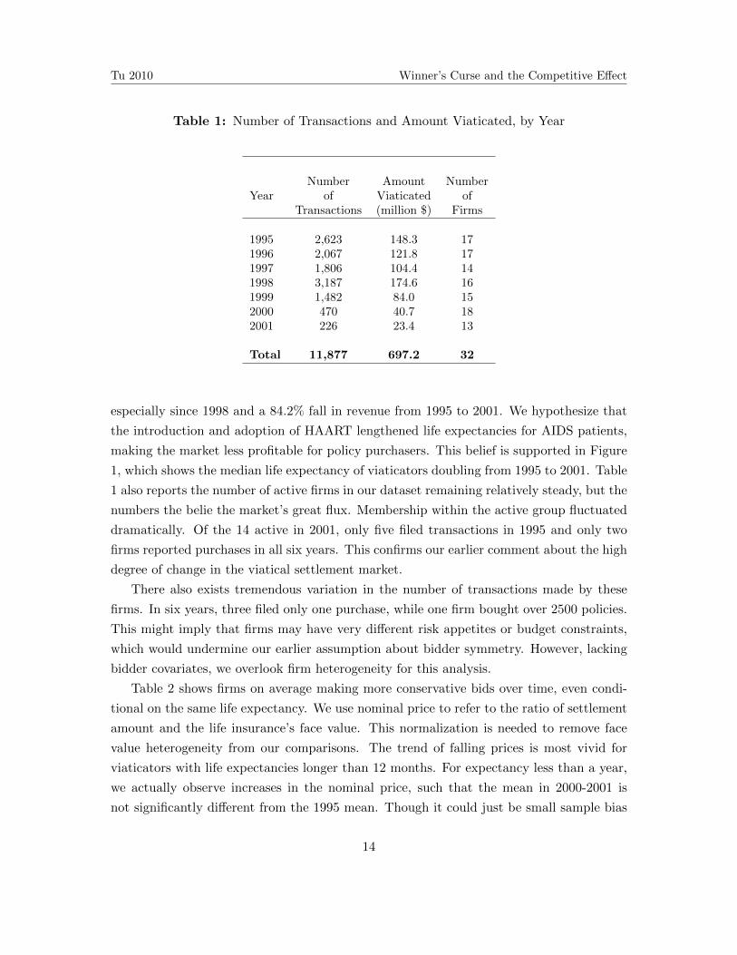
Tu 2010 Winner’s Curse and the Competitive Effect
Table 1: Number of Transactions and Amount Viaticated, by Year
YearNumber Amount Number
of Viaticated ofTransactions (million $) Firms
1995 2,623 148.3 171996 2,067 121.8 171997 1,806 104.4 141998 3,187 174.6 161999 1,482 84.0 152000 470 40.7 182001 226 23.4 13
Total 11,877 697.2 32
especially since 1998 and a 84.2% fall in revenue from 1995 to 2001. We hypothesize that
the introduction and adoption of HAART lengthened life expectancies for AIDS patients,
making the market less profitable for policy purchasers. This belief is supported in Figure
1, which shows the median life expectancy of viaticators doubling from 1995 to 2001. Table
1 also reports the number of active firms in our dataset remaining relatively steady, but the
numbers the belie the market’s great flux. Membership within the active group fluctuated
dramatically. Of the 14 active in 2001, only five filed transactions in 1995 and only two
firms reported purchases in all six years. This confirms our earlier comment about the high
degree of change in the viatical settlement market.
There also exists tremendous variation in the number of transactions made by these
firms. In six years, three filed only one purchase, while one firm bought over 2500 policies.
This might imply that firms may have very different risk appetites or budget constraints,
which would undermine our earlier assumption about bidder symmetry. However, lacking
bidder covariates, we overlook firm heterogeneity for this analysis.
Table 2 shows firms on average making more conservative bids over time, even condi-
tional on the same life expectancy. We use nominal price to refer to the ratio of settlement
amount and the life insurance’s face value. This normalization is needed to remove face
value heterogeneity from our comparisons. The trend of falling prices is most vivid for
viaticators with life expectancies longer than 12 months. For expectancy less than a year,
we actually observe increases in the nominal price, such that the mean in 2000-2001 is
not significantly different from the 1995 mean. Though it could just be small sample bias
14

Tu 2010 Winner’s Curse and the Competitive Effect
Figure 1: Life Expectancy of Viaticators from 1995 to 2001
*: 25th percentile; o: 50th percentile; +: 75th percentile
(n = 52), the aberrant increase may also be an unexpected consequence of HAART. In
general, HAART elongated life expectancies, but for patients whose illness had either pro-
gressed too far for HAART or were otherwise resistant to the treatment, the post-1995
technological improvements had no impact. For these sickliest of individuals having ex-
hausted their treatment options, uncertainty about their expected time of death would
have been very low, which could drive higher nominal prices. Other trends in Table 2
support this hypothesis. Notice that for life expectancy buckets of greater than two years,
number of transactions actually rose before the market’s near dissolution in 2000-2001. On
the other hand, the number of policies sold with expectancies under a year declined, even
with the sudden spike in transactions in 1998 (see Table 1). One explanation for this is
that viaticators who in 1995 would have fallen into the < 12 bucket because of HAART
extended their life expectancies and instead fell into a healthier bucket. Thus, the few pol-
icy sellers that remained in the most sickly cohort were the ones whose deaths were most
imminent and least uncertain. In sum, the success of HAART could have acted as a sieve
15
Tu 2010 Winner’s Curse and the Competitive Effect
to differentiate out patients with the highest mortality risk, and this plausibly explains why
nominal price for viaticators with life expectancy < 12 defied the overall industry decline
in settlement values.
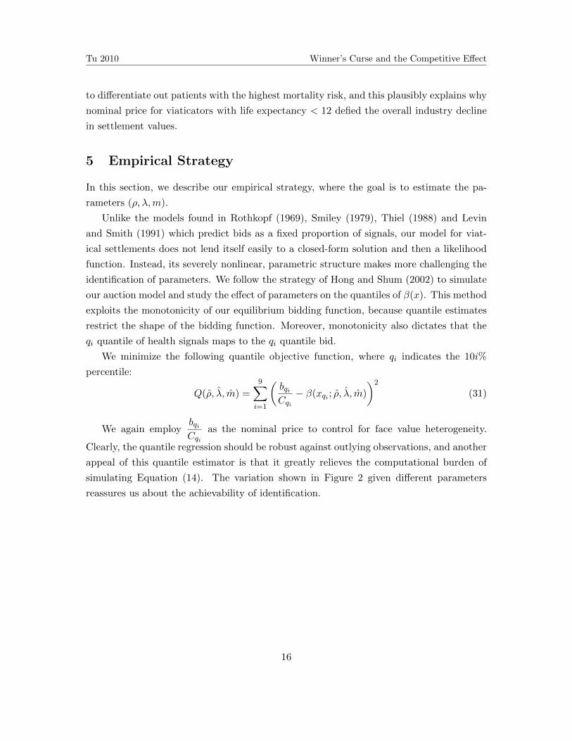
5 Empirical Strategy
In this section, we describe our empirical strategy, where the goal is to estimate the pa-
rameters (ρ, λ,m).
Unlike the models found in Rothkopf (1969), Smiley (1979), Thiel (1988) and Levin
and Smith (1991) which predict bids as a fixed proportion of signals, our model for viat-
ical settlements does not lend itself easily to a closed-form solution and then a likelihood
function. Instead, its severely nonlinear, parametric structure makes more challenging the
identification of parameters. We follow the strategy of Hong and Shum (2002) to simulate
our auction model and study the effect of parameters on the quantiles of β(x). This method
exploits the monotonicity of our equilibrium bidding function, because quantile estimates
restrict the shape of the bidding function. Moreover, monotonicity also dictates that the
qi quantile of health signals maps to the qi quantile bid.
We minimize the following quantile objective function, where qi indicates the 10i%
percentile:
Q(ρ, λ, m) =9∑i=1
(bqiCqi− β(xqi ; ρ, λ, m)
)2
(31)
We again employbqiCqi
as the nominal price to control for face value heterogeneity.
Clearly, the quantile regression should be robust against outlying observations, and another
appeal of this quantile estimator is that it greatly relieves the computational burden of
simulating Equation (14). The variation shown in Figure 2 given different parameters
reassures us about the achievability of identification.
16

Tu 2010 Winner’s Curse and the Competitive Effect
Table 2: Average Nominal Price and Life Expectancy of a Viatical Settlement, by LifeExpectancy and Year
Life Expectancy1995 1996-1997 1998-1999 2000-2001
(months)
<12
Nominal Price (%) 73.59 78.62 68.20 73.2395% CI [72.77 , 74.42] [77.84 , 79.40] [66.05 , 70.35] [70.42 , 75.94]std error 0.420 0.397 1.093 1.350
Life Expectancy 7.592 8.192 7.878 8.276std error 0.107 0.120 0.153 0.307
n 373 445 273 53
12-23
Nominal Price (%) 71.43 71.34 60.08 50.6095% CI [71.00 , 71.86] [70.74 , 71.94] [59.35 , 60.82] [47.76 , 53.45]std error 0.217 0.306 0.373 1.440
Life Expectancy 15.761 16.377 15.656 16.207std error 0.096 0.104 0.107 0.283
n 1202 1223 1099 142
24-35
Nominal Price (%) 61.65 60.74 48.24 38.9995% CI [61.01 , 62.29] [59.84 , 61.64] [47.50 , 48.98] [36.52 , 41.46]std error 0.324 0.457 0.378 1.249
Life Expectancy 25.302 27.541 25.730 26.651std error 0.100 0.136 0.088 0.321
n 624 703 1257 132
36-47
Nominal Price (%) 48.72 46.92 36.25 29.8695% CI [47.02, 50.41] [46.14 , 47.69] [35.49 , 37.01] [27.93 , 31.80]std error 0.860 0.397 0.386 0.981
Life Expectancy 37.728 37.096 36.849 36.721std error 0.196 0.082 0.066 0.150
n 212 1026 1152 195
≥48
Nominal Price (%) 39.31 36.13 28.86 26.9195% CI [36.90 , 41.72] [34.70 , 37.56] [28.00 , 29.73] [24.86 , 28.97]std error 1.222 0.729 0.441 1.039
Life Expectancy 55.066 56.062 58.281 58.250std error 0.672 0.553 0.694 0.927
n 212 492 888 154
17

Tu 2010 Winner’s Curse and the Competitive Effect
Figure 2: Bids with Different Parameters
o: ρ = 3, λ = 0.1, m = 0.5; +:ρ = 3, λ = 0.5, m = 1; +:ρ = 3, λ = 1, m = 3; :ρ = 3,λ = 1.5, m = 1.5
The delta estimation strategy we use to calculate standard errors is explored in the
Appendix.
6 Results
Our estimates are presented in Table 3 and graphed in Figure 3 on page 19.
18

Tu 2010 Winner’s Curse and the Competitive Effect
Table 3: Parameter Estimates
1995 1996-1997 1998-1999 2000-2001
ρ 4.592 4.468 3.329 2.9911(1.279) (0.091) (0.224) (0.146)
λ 0.698 0.878 0.797 0.873(0.154) (0.022) (0.061) (0.075)
m 0.756 1.174 1.127 1.125(0.172) (0.057) (0.112) (0.091)
n 2623 3889 4669 696
Figure 3: Predicted Bids
o: 1995; *: 1996-1997; +: 1998-1999; : 2000-2001
These results capture the trends we observed previously. Bids conditional on the same
19

Tu 2010 Winner’s Curse and the Competitive Effect
life expectancy are falling over time, except transactions between 1996-1997 for higher
mortality risk settlements. Yet, we predict that 1995 bids are higher than 1996-1997 bids
for life expectancies greater than 32 months. We see this as evidence of rising uncertainty
about the life expectancy readings of the healthier viaticators, as captured in our joint
distribution. This rising uncertainty also manifests as more negative slopes for 1998-1999
and 2000-2001 bid functions. Conversely, bids for the most sickly appear not to have
fallen significantly, which agrees with the data and our hypothesis that HAART helped
differentiate between risky and less risky policies.
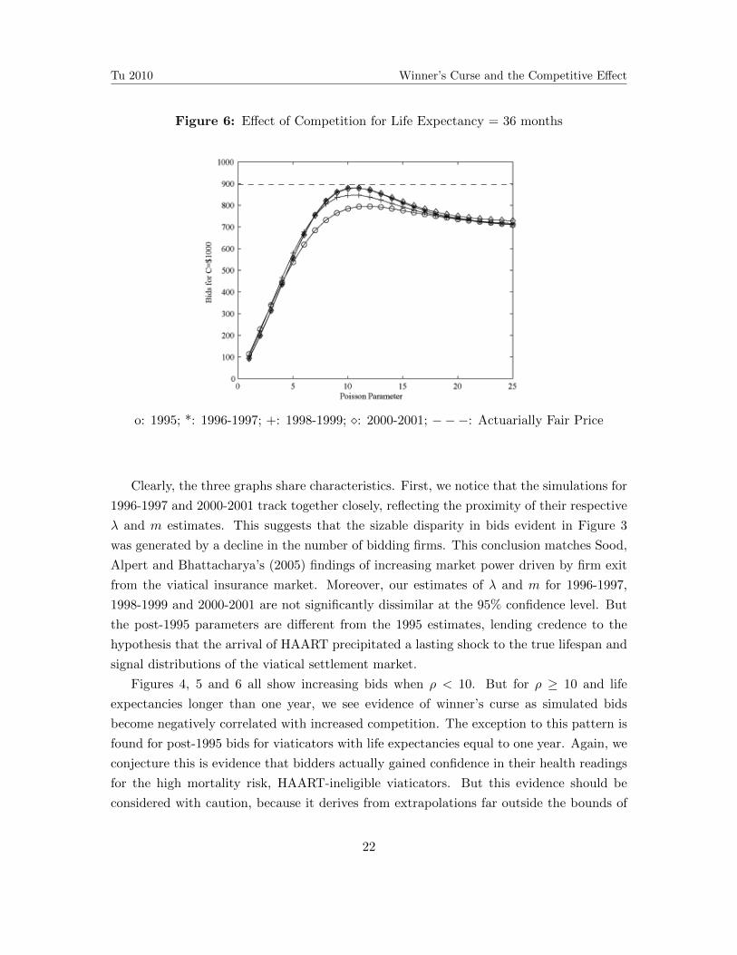
6.1 Effect of Increased Competition
We next address claims that purchasers in the viatical market exploited market power to
offer viaticators lower than actuarially fair prices. We also test Paarsch’s prediction that
in common value auctions, increasing the number of bidders drives prices upward initially
but then causes bids to drop as fears of the winner’s curse supersede the competitive effect
(1992). Since our analysis treats number of bidders as unobserved, we rely on comparative
statics on our poisson parameter ρ to investigate market power.
Figures 4, 5 and 6 show simulated bids in response to increasing ρ, conditional on
different life expectancies. We also plot the actuarially fair price AFP , which is calculated
using D = time of death and an annual insurance premium z. We continue to model life
expectancy using an exponential distribution.
AFP =
∫ ∞0
P [D = t]
[C
(1 + r)t− zt
]dt (32)
20

Tu 2010 Winner’s Curse and the Competitive Effect
Figure 4: Effect of Competition for Life Expectancy = 12 months
o: 1995; *: 1996-1997; +: 1998-1999; : 2000-2001; −−−: Actuarially Fair Price
Figure 5: Effect of Competition for Life Expectancy = 24 months
o: 1995; *: 1996-1997; +: 1998-1999; : 2000-2001; −−−: Actuarially Fair Price
21
Tu 2010 Winner’s Curse and the Competitive Effect
Figure 6: Effect of Competition for Life Expectancy = 36 months
o: 1995; *: 1996-1997; +: 1998-1999; : 2000-2001; −−−: Actuarially Fair Price
Clearly, the three graphs share characteristics. First, we notice that the simulations for
1996-1997 and 2000-2001 track together closely, reflecting the proximity of their respective
λ and m estimates. This suggests that the sizable disparity in bids evident in Figure 3
was generated by a decline in the number of bidding firms. This conclusion matches Sood,
Alpert and Bhattacharya’s (2005) findings of increasing market power driven by firm exit
from the viatical insurance market. Moreover, our estimates of λ and m for 1996-1997,
1998-1999 and 2000-2001 are not significantly dissimilar at the 95% confidence level. But
the post-1995 parameters are different from the 1995 estimates, lending credence to the
hypothesis that the arrival of HAART precipitated a lasting shock to the true lifespan and
signal distributions of the viatical settlement market.
Figures 4, 5 and 6 all show increasing bids when ρ < 10. But for ρ ≥ 10 and life
expectancies longer than one year, we see evidence of winner’s curse as simulated bids
become negatively correlated with increased competition. The exception to this pattern is
found for post-1995 bids for viaticators with life expectancies equal to one year. Again, we
conjecture this is evidence that bidders actually gained confidence in their health readings
for the high mortality risk, HAART-ineligible viaticators. But this evidence should be
considered with caution, because it derives from extrapolations far outside the bounds of
22

Tu 2010 Winner’s Curse and the Competitive Effect
our data.
Instead, the most striking observation is that all our estimates through 1995-2001 fall in
the strictly increasing region across all three life expectancies. Realized settlement values
are well below the actuarially fair price, and more competition would cause settlement
values to grow dramatically. This supports claims that viatical firms enjoyed market power,
enabling them to extract surpluses from policy sellers. This analysis also provides empirical
evidence that despite the common value nature of this auction, winner’s curse did not play
a role in affecting bidding behavior.
7 Conclusion
We have conceptualized transactions in the viatical settlement market from 1995-2001
as first-price, common value auctions. By applying a simulated quantile non-linear least
squares estimation to our parametric model, we observe that the market experienced in a
lasting shock between 1995 and 1996, likely due to the introduction of HAART, which dra-
matically extended the life expectancy of HIV/AIDS patients. Our analysis also suggests
that throughout the six-year period, viatical firms exercised market power that allowed
them to underprice their purchases. Over time, this market power actually increased as
a result of firm exit, but market consolidation also coincided with a significant decline in
market size.
Our analysis should not necessarily be read as advocating price floors for the viatical
market. Such regulation would likely be too heavy-handed and inflexible for this mar-
ket’s complexities and need to rapidly react to technological improvements. Bhattacharya,
Goldman and Sood (2004) have claimed that price floors would reduce social welfare by
blocking potential pareto-improving transactions. However, more competition in this mar-
ket should have been encouraged, and it warrants further study to assess whether the
growing life settlement market also suffers analogously from imperfect competition.
In this paper’s introduction, we set forth to propose a novel strategy for evaluating the
level of competition in a given market. We have done this for the viatical insurance market
and discovered that on average, transactions for life insurance policies between 1995 and
2001 had fewer than five bidders. At that level, we did not see evidence of winner’s curse,
since any impact was completely eclipsed by the competitive effect. This conclusion drawn
from our model is striking in and of itself, but it also augurs the more general application
of our methodology for measuring competition in other markets wherever the object for
sale has a common but unknown value.
23

Tu 2010 Winner’s Curse and the Competitive Effect
8 Appendix: Calculation of Standard Errors
We apply a delta estimation procedure to calculate our standard errors. For θ = (ρ, λ,m),
our objective function in Equation (31) can be rewritten with the following matrix multi-
plication, where g(θ) gives the predicted quantile bids and y represents the actual quantile
nominal prices from our dataset. Since we are considering the ten-percentiles, both g(θ)
and y are 9× 1 matrices.
(ρ, λ, m) = minθ
(g(θ)− y
)′I(g(θ)− y
)We take the first order condition, and let H(θ) be the Jacobian matrix of g(θ). We denote
the true population parameters as θ0.
0 = H(θ)′I(g(θ)− y
)0 ≈ H(θ)′I
[g(θ0)− y +H(θ)(θ − θ0)
]by Taylor approximation
H(θ)′I[H(θ)(θ − θ0)
]= H(θ)I (g(θ0)− y)
θ − θ0 =[H(θ)′IH(θ)
]−1H(θ)′ (g(θ0)− y)
V ar(θ − θ0) = V ar(θ) =[H(θ)′IH(θ)
]−1H(θ)′V ar [g(θ0)− y]
[[H(θ)′IH(θ)
]−1H(θ)′
]′So it suffices to find V ar [g(θ0)− y], which is a 9 × 9 variance-covariance matrix, and by
Newey and McFadden (1994) and Paarsch (1994), we note that
√n [y − g(θ0)] −→ N(0,Ω)
To find Ω, we first introduce a kernel density function f(x), which denotes the density of
the error distribution at different quantiles (Koenker and Hallock 2000). Here, n is the
number of observations, q is the number of estimated quantiles and h is a bandwidth term
we find by assuming the underlying Guassian errors and minimizing the asymptotic mean
integrated squared error.
f(x) =1
qh
q∑i=1
1√2π
exp
[(x− xi)2)
2h2
]
24
Tu 2010 Winner’s Curse and the Competitive Effect
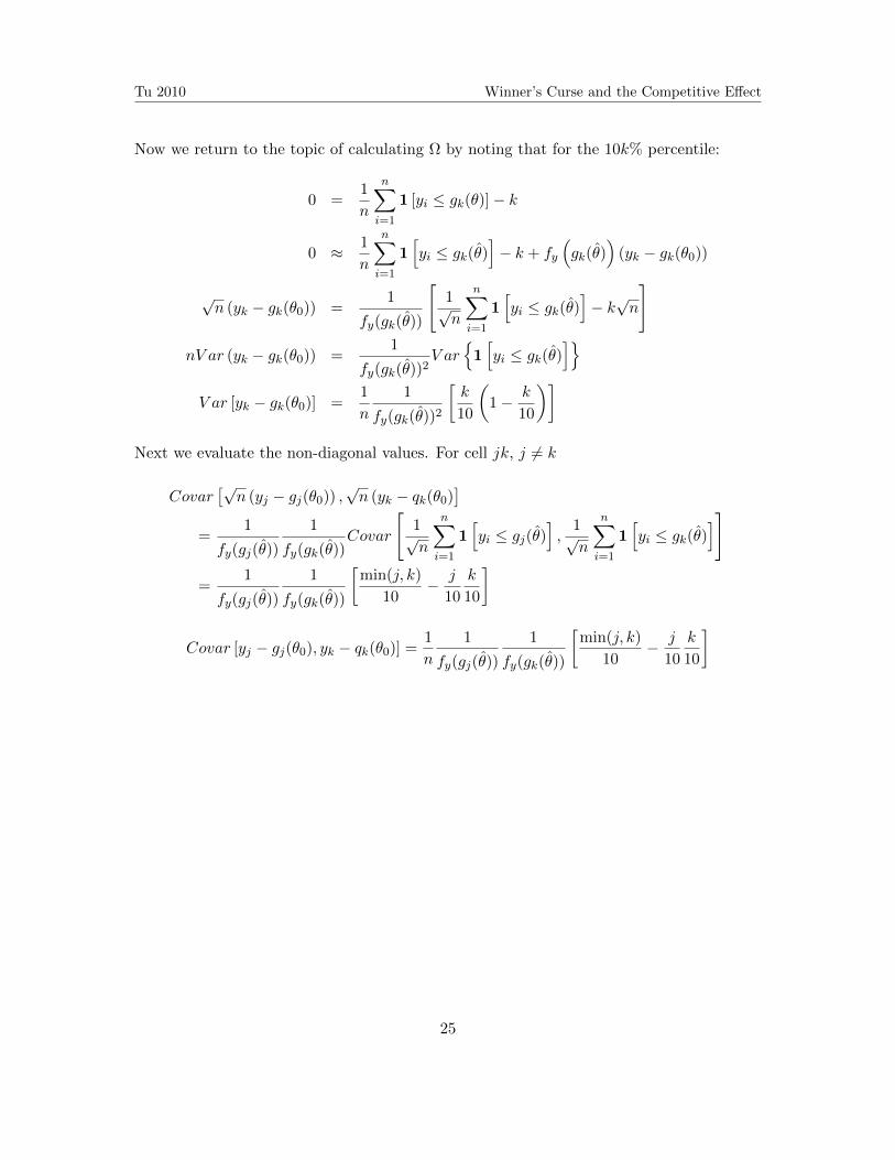
Now we return to the topic of calculating Ω by noting that for the 10k% percentile:
0 =1
n
n∑i=1
1 [yi ≤ gk(θ)]− k
0 ≈ 1
n
n∑i=1
1[yi ≤ gk(θ)
]− k + fy
(gk(θ)
)(yk − gk(θ0))
√n (yk − gk(θ0)) =
1
fy(gk(θ))
[1√n
n∑i=1
1[yi ≤ gk(θ)
]− k√n
]
nV ar (yk − gk(θ0)) =1
fy(gk(θ))2V ar
1[yi ≤ gk(θ)
]V ar [yk − gk(θ0)] =
1
n
1
fy(gk(θ))2
[k
10
(1− k
10
)]Next we evaluate the non-diagonal values. For cell jk, j 6= k
Covar[√n (yj − gj(θ0)) ,
√n (yk − qk(θ0)
]=
1
fy(gj(θ))
1
fy(gk(θ))Covar
[1√n
n∑i=1
1[yi ≤ gj(θ)
],
1√n
n∑i=1
1[yi ≤ gk(θ)
]]
=1
fy(gj(θ))
1
fy(gk(θ))
[min(j, k)
10− j
10
k
10
]
Covar [yj − gj(θ0), yk − qk(θ0)] =1
n
1
fy(gj(θ))
1
fy(gk(θ))
[min(j, k)
10− j
10
k
10
]
25

Tu 2010 Winner’s Curse and the Competitive Effect
References
Akerlof, George. 1970. “The Market for Lemons: Quality Uncertainty and the MarketMechanism,” Quarterly Journal of Economics, 84(3), 488-500.
Armantier, Olivier. 2002. “Deciding between the Common and Private Values Paradigm:An Application to Experimental Data,” International Economic Review, 43(3), 783-801.
Belth, Joseph. 2000. “Viatical and Life Settlement Transactions: The Frightening Sec-ondary Market for Life Insurance Policies,” Contingencies, March/April, 22-25.
Bhattacharya, Jay, Dana Goldman and Neeraj Sood. 2001. ”The Decision to Sell LifeInsurance,” MIMEO, RAND.
——————–. 2004. “Price Regulation in Secondary Insurance Markets.” The Journalof Risk and Insurance, 71(4), 643-675.
Bulow, Jeremy and Paul Klemperer. 2002. “Prices and Winner’s Curse,” RAND Journalof Economics, 33(1), 1-21.
Cawley, John and Tomas Philipson. 1999. “An Empirical Examination of InformationBarriers to Trade in Insurance.” The American Economic Review, 89(4), 827-846.
Goldstein, Matthew. 2007. “Profiting from Mortality: Death bonds may be the mostmacabre investment scheme ever devised by Wall Street,” BusinessWeek, July 30.
Harrison, Glenn and John List. 2008. “Naturally Occuring Markets and Exogenous Lab-oratory Experiments: A Case Study for the Winner’s Curse,” The Economic Journal,119(April), 822-843.
Hendricks, Kenneth, Joris Pinkse and Robert Porter. 2003. “Empirical Implications ofEquilibrium Bidding in First-Price, Symmetric, Common-Value Auctions,” The Review ofEconomic Studies, 70(1), 115-145.
Hong, Han and Matthew Shum. 2002. “Increasing Competition and the Winner’s Curse:Evidence from Procurement,” Review of Economic Studies, 69(Oct 2002), 871-898.
Kagel, John and Dan Levin. 2002. Common Value Auctions and the Winner’s Curse,Princeton: Princeton University Press.
Koenker, Roger and Kevin Hallock. 2001. ”Quantile Regression: An Introduction,” Jour-nal of Economic Perspectives, 15(4), 143-156.
26

Tu 2010 Winner’s Curse and the Competitive Effect
Levin, Dan and James Smith. 1991. ”Some Evidence on the Winner’s Curse: Comment,”The American Economic Review, 81(1), 370-375.
Life Insurance Settlement Association (LISA). 2007. “Data Collection Report: 2004-2005,”http://www.lisaassociation.org.
Milgrom, Paul. 1979. “A Convergence Theorem for Competitive Bidding with DifferentialInformation,” Econometrica, 47, 679-688.
Milgrom, Paul and Robert Weber. 1982. “A Theory of Auctions and Competitive Bid-ding,” Econometrica, 50(5), 1089-1122.
Newey, Whitney and Daniel McFadden. 1994. “Large Sample Estimation and HypothesisTesting,” R.F. Engle and D.L. McFadden, eds., Handbook of Econometrics, Vol. 4, NorthHolland: Elsevier, 2112-2245.
Paarsch, Harry. 1992. “Deciding between the common and private value paradigms inempirical models of auctions.” Journal of Econometrics, 51, 191-215.
——————–. 1994. “A Comparison of Estimators for Empirical Models of Auctions,”Annales d’conomie et de Statistique, 34 (April 1994), 143-157.
Paarsch, Harry and Han Hong. 2006. An Introduction to the Structural Econometrics ofAuction Data. Cambridge: MIT Press.
Quinn, Sarah. 2008. “The Transformation of Morals in Markets: Death, Benefits, and theExchange of Life Insurance Policies.” American Journal of Sociology, 114(3), 738-780.
Rothkpof, Michael. 1969. “A Model of Rational Bidding,” Management Science, 18(7),362-373.
Smiley, Albert. 1979. Competitive Bidding Under Uncertainty: the Case of Offshore Oil.Cambridge: Ballinger Publishing Company.
Sood, Neeraj, Abby Alpert and Jay Bhattacharya. 2005. “Technology, Monopoly and theDecline of the Viatical Settlements Industry.” NBER Working Paper 11164.
Tergesen, Anne. 2008. ”Source of Cash for Seniors is Drying Up,” The Wall Street Journal,November 13.
Thiel, Stuart. 1988. “Some Evidence on the Winner’s Curse,” American Economic Review,78, 884-895.
27

Tu 2010 Winner’s Curse and the Competitive Effect
Trinkaus, John and Joseph Giacalone. 2002. “Entrepreneurial ’Mining’ of the Dying:Viatical Transactions, Tax Strategies and Mind Games,” Journal of Business Ethics, 36,187-194.
Wilson, Robert. 1977. “A Bidding Model of Perfect Competition,” Review of EconomicStudies, 44, 511-518.
Wolk, Gloria Grening. 1997. Cash for the Final Days: A Financial Guide for the Termi-nally Ill and Their Advisors. Laguna Hills: Balkin Books.
28