The Winner’s Curse - European Banking Authority Pausch...The Winner’s Curse Evidence on the...

The Winner’s Curse∗

Evidence on the Danger ofAggressive Credit Growth in Banking

Thomas Kick Thilo Pausch Benedikt Ruprecht

September 22, 2015

Abstract

Excessive credit creation by banks was at the root of the recent financial crisis. Nev-ertheless, micro-prudential regulation lacks a clear methodology to identify thesebanks. Combining arguments from banking and auction theory, we show thatoveroptimism causes excessive lending, subsequently yielding abnormal loan write-offs. We propose a new measure of excessive credit growth known from macroe-conomics to identify credit booms and test our model for German bank and bank-portfolio level data. Unlike traditional measures of (excessive) loan growth, our newmeasure identifies banks that are affected by abnormal loan write-offs, need capitalsupport, or default in subsequent years.

Keywords: Excessive credit growth, Winner’s Curse, Loan-to-GDP gap, Micro-prudential regulation, Identifying weak banks

JEL classification: C23, G21, G32.

∗Contact address: Deutsche Bundesbank, P.O. Box 10 06 02, 60006 Frankfurt, Germany.Phone: +49 69 9566 8194. E-Mail: [email protected], [email protected],[email protected]. The authors thank Hans Degryse, Klaus Dullmann, Rainer Hasel-mann, Christoph Memmel, Klaus Schaeck, Weidong Tian, as well as participants at the 2013 EEA-ESEMConference (Gothenburg), the 2014 MFA Meetings (Orlando), the 2014 SUERF Colloquium and BAFFIFinlawmetrics Conference (Bocconi), the 2014 Swiss Society for Financial Market Research Conference(Zurich), the 2015 WEAI/IBEFA meeting (Honolulu) and participants at the Bundesbank Seminar onBanking and Finance for their valuable input. This discussion paper represents the authors’ personalopinions and does not necessarily reflect the views of the Deutsche Bundesbank or its staff.

1 Introduction

Excessive credit and asset growth has been a major driver of the recent financial crisis(e.g., Mian and Sufi, 2009). When too many banks follow the same common strategy— for example due to competition (e.g., Gorton and He, 2008; Aikman et al., 2015) —lending standards are lowered in order to attract more borrowers and a credit boom arises.But how can loan growth be characterized as excessive in advance before a bank fails?Regulators tried to restrict excessive credit growth in the new Basel III capital frameworkby introducing countercyclical buffers as a macro-prudential tool to prevent the build-upof systemic risk (BCBS, 2011)1 or by demanding countercyclical loan loss provisioning(Jimenez and Saurina, 2006; Jimenez et al., 2014b). These approaches increase banks’minimum capital requirements and simultaneously lower banks’ excess capital which mightbe used to fund additional loans. BCBS (2010) offers guidance when credit growth at anational level increases too much and the countercyclical capital buffer should be acti-vated. However, at a micro-prudential level supervisors lack measures to gauge when anindividual bank has become vulnerable due to excessive lending.

Therefore, we focus on identifying weak banks with excessive credit growth as mo-tivated by (BCBS, 2015). Our paper makes three contributions to the nexus betweenexcess credit growth and subsequent losses through loan charge-offs and potential bankdefault. First, we offer a new simple theoretical argument for why some banks engage inexcessive credit growth as a consequence of a Winner’s Curse situation even though creditrationing in the sense of Stiglitz and Weiss (1981) and Williamson (1987) is still presentin the aggregate credit market. Second, we propose a new methodology to measure ex-cessive credit growth at the bank level. Our approach is based on methods of estimatingaggregate credit gaps at the national level (e.g., Mendoza and Terrones, 2008, 2012) andconsistent with the method proposed by BCBS (2010).2 Specifically, we estimate excesscredit growth as the difference between real loan growth and its long term trend, wherethe trend is derived from the Hodrick-Prescott (HP) filter. Third, we use a unique regula-tory data set that allows us to identify write-offs (following credit growth) not only at thebank level, but also at the portfolio level to test the results of our model. We find thatbanks identified as excessive credit suppliers — either with respect to total credit or theirmajor sectoral portfolios — will incur disproportionately large write-offs in subsequentyears. Furthermore, excessive credit suppliers are more likely to default and to receivecapital support in later years. Therefore, our method is a useful tool for micro-prudentialsupervisors to identify endangered institutions and can be used to justify capital chargesin excess of the minimum requirements of Basel III under the Supervisory Review Processof Pillar 2.

To develop our simple theoretical model, we combine arguments from the literatureon banking and auction theory to explain why some banks excessively expand credit. Weargue that there exists a kind of Winner’s Curse in credit markets. At the time when

1The Accord states: As witnessed during the financial crisis, losses incurred in the banking sectorduring a downturn preceded by a period of excess credit growth can be extremely large. Such losses candestabilize the banking sector [,...]. (BCBS, 2011, paragraph 29). National authorities can demand aCommon Equity Tier 1 ratio of up to 2.5% of risk-weighted assets.

2National authorities consider the macroeconomic credit-to-GDP gap when deciding about the levelof the countercyclical buffer. The gap is determined as the difference between actual credit-to-GDP ratioand its long-term trend, which is calculated using the Hodrick-Prescott filter (BCBS, 2010).

2

banks make lending decisions, they need to evaluate the general level of credit risk in theaggregate lending market. Being too optimistic encourages the bank to extend more newloans than would be optimal. That is, banks may find themselves in a situation wherelending and credit risk turn out to be excessive ex post, causing extremely high rates ofloan default. Interestingly, the intention to ration credit does not protect banks againstexcessive future loan losses.

We test the predictions of our model by analyzing the relationship between past mea-sures of (excess) loan growth and proxies for ex post credit risk, i.e. loan write-offs,using prudential data from Germany. Germany did not experience a credit boom overthe last two decades. Nevertheless, individual banks have expanded their balance sheetsand encountered distress or even collapsed. Hence, our data set is well-suited to identifythose banks that engage in excessive lending as a rather small group compared to thewhole banking system. Using a unique data set of bank loan portfolio data, we applythe HP filter to decompose a bank’s loan growth into a trend and a cyclical component.Excessive credit growth is defined as a cyclical component, i.e. the difference betweenactual growth and the long term trend in credit growth. As our data set contains loancharge-offs for different lending sectors, we conduct our analysis for both total lendingand lending at a sectoral loan portfolio level where we investigate banks’ three largestlending portfolios. Using traditional measures of (excessive) loan growth, we show thatthe majority of banks are doing well in extending credit supply; i.e. banks are basicallymonitoring loan exposures sufficiently and do not lend excessively. Based on excessivecredit growth measures derived from the HP filter, we identify those banks that extendtoo much credit and therefore experience significantly higher loan-write offs.

Our paper contributes to the empirical and theoretical literature linking excessivecredit growth and future loan losses. Salas and Saurina (2002), Jimenez and Saurina(2006), and Foos et al. (2010) all find a positive relationship between abnormal creditgrowth and loan losses in subsequent years, but differ in the time lag between lending ex-pansion and loan defaults. Jimenez and Saurina (2006) find that the major driver behindexcessive credit growth is banks lowering their credit standards during boom periods. Adeterioration in lending standards can be the product of bank managers’ herding behav-ior (Rajan, 1994), increased collateral values during boom periods (Asea and Blomberg,1998), the general opaqueness of information on borrowers’ creditworthiness (Dell’Aricciaand Marquez, 2006), or macroeconomic drivers such as low interest rates, i.e. the risk-taking channel of monetary policy (Dell’Ariccia et al., 2014; Jimenez et al., 2014a). Also,interbank competition can induce lower credit standards and fuel credit cycles (Gortonand He, 2008; Aikman et al., 2015). Broecker (1990) and Shaffer (1998) address theproblem of competition when new banks enter the market and find that borrowers’ loanquality decreases with the number of banks previously rejected loan applicants can applyat.

Another strand of the empirical literature focuses on credit expansion (and contrac-tion) as a consequence of the procyclical behavior of loan-loss provisioning and capitalrequirements (e.g., Laeven and Majnoni, 2003; Bikker and Metzemakers, 2005; Behn et al.,2015). Although credit risk builds up during booms, banks delay loan-loss provisioningfor too long, and therefore have to write off a disproportionately large volume of loansduring recessions (Laeven and Majnoni, 2003). Berger and Udell (2004) see the cause ofthe procyclicality of bank lending in the “institutional memory hypothesis.” Institutions

3

forget about prior loan defaults, as older loan officers are replaced with officers who havenever experienced a crisis. As a consequence, as more and more time passes since the lastcrisis, banks lower their credit standards and attract more borrowers of poor quality.

A small literature provides evidence at the bank level on how the enforcement ofregulations can mitigate credit growth. Aiyar et al. (2014) investigate the time-varyingbank-specific capital requirements imposed by the UK Financial Services Authority un-der the Basel I regime. The authors find that higher capital requirements reduce lendinggrowth for regulated banks, whereas the opposite holds for unregulated banks. Jimenezet al. (2014b) investigate the impact of the dynamic loan loss provisioning regime inSpain on credit supply. They find that countercyclical dynamic provisioning mitigatescredit supply cycles, but firms switch to receive credit supply from banks not coveredunder the provisioning scheme. Besides this form of regulatory arbitrage, affected bankslend to riskier borrowers during booms. Basten and Koch (2014) investigate the rates de-manded by banks after the activation of the countercyclical capital buffer in Switzerlandin February 2013. Capital-constraint banks with less excess capital are found to increasemortgage rates relatively more and rates to highly levered borrowers are increased overpro-portionally. While banks demand higher loan rates, the activation of the countercyclicalcapital buffer does not impact banks’ willingness to accept new mortgage loans.

The remainder of this paper is organized as follows: Section 2 links the credit supplyliterature with auction pricing theory to provide the foundation of our Winner’s Curseargument. Section 3 presents some institutional background on the German bankingsector and explains the data and methodology underlying our empirical analysis. Resultsare presented in Section 4. Section 5 concludes.

2 Theoretical foundation of the argument

From the post-crisis perspective, the question arises as to why banks engage in excessivelending, subsequently leading to high loan charge-offs. Williamson (1987) shows thatbanks’ expected cash flows from offering a standard debt contract decline when the nomi-nal loan rate is set too high (i.e. sufficiently close to a borrower’s maximum ability to pay)due to an increasing probability of borrower default. As a consequence, in a situation ofcostly state verification with ex-ante identical borrowers, a backward bending loan supplyfunction and credit rationing appear due to the nature of an optimal loan contract design.In more formal terms: a bank’s expected profit from lending rises in the nominal paymentobligation R on loans as long as the payment obligation does not exceed a given thresh-old level R∗. Beyond R∗ the expected profit falls when the nominal payment obligationis increased. This effect translates into a backward bending loan supply function whichreaches a maximum at R∗.3

Given that both the common design of loan contracts as well as asymmetric informa-

3Stiglitz and Weiss (1981) present an alternative argument for the existence of backward bendingloan supply functions based on asymmetric information about the quality of borrowers. When potentialborrowers differ with respect to their individual risk levels and ability to meet payment obligations,adverse selection drives good borrowers out of the market if they are offered a standard debt contract. Asa result, the average credit quality of the bank’s loan portfolio decreases when loan supply is expanded. Toa certain degree, banks are able to over-compensate this adverse selection effect by increasing borrowers’payment obligations. However, beyond a certain threshold the adverse selection effect dominates.

4

tion cause backward bending loan supply functions it cannot be optimal for individualbanks to increase lending beyond the volume corresponding to the threshold paymentobligation R∗. Additionally, credit rationing is also, at first glance, not compatible withexcessive lending. Our model therefore combines banking theory, auction theory and de-cision making in situations of risk. We show that, regardless of the existence of creditrationing, uncertainty with respect to the general level of credit risk in the market distortsbanks’ lending decisions. This causes a Winner’s Curse: a single bank’s assessment ofthe general risk level turns out too optimistic ex post, resulting in excessive lending andextremely high write-offs on loans.

For a more formal representation of the argument we build on Williamson (1987): con-sider a credit market with a large number of ex-ante identical borrowers who need externalfunds to finance a profitable investment project with an uncertain outcome. Banks providecredit by offering identical standard debt contracts with a nominal payment obligationR to borrowers. That is, a representative borrower has to make a predefined repaymentR to the bank when the debt contract matures. If, however, the borrower is not able tomake this repayment, the bank takes possession of all available outcome of the borrower’sproject and incurs some fixed cost γ to monitor the project. Let F (x|s) and f(x|s) > 0denote the cumulative probability distribution function and the probability density func-tion of the outcome x of a representative borrower’s investment project conditional onthe general level of risk s in the credit market.4 The bank’s expected profit from such astandard debt contract E(π(x|s)) amounts to:

E(π(x|s)) =

∫ R

0

(x− γ) dF (x|s) +R (1− F (R|s)) . (1)

There exists a certain R∗ which maximizes E(π(x|s)). For all R > R∗ the functionE(π(x|s)) is backward bending. That is, differentiating (1) with respect to R yields

d

dRE(π(x|s)) = (1− F (R|s))− γf(R|s). (2)

Due to F (R|s) ∈ [0, 1] and γ, f(R|s) > 0 there exists a certain R∗ for which the right-handside of (2) becomes zero. Furthermore, the common features of cumulative probabilitydistribution functions imply that d

dRE(π(x|s)) is positive (negative) for R < R∗ (R > R∗).

If we further assume that a bank’s loan supply function L is an increasing function ofthe expected (conditional) profit of a representative standard debt contract, i.e.

L ≡ L (E(π(x|s))) with L′(·) ≡ d

dE(·)L (E(π(x|s))) > 0, (3)

then the previous observations translate into a backward-bending loan supply function ofa bank with L′(·) ≥ (<)0 for R ≤ (>)R∗ and L′(·) = 0 for R = R∗. However, from (3) oneeasily observes that a bank’s loan supply depends not only on R, but also on the generalrisk level s in the credit market. The risk level s represents a number of factors in the(macro) economic environment of borrowers with an impact on their project outcomeswhich they cannot directly affect by their behavior.

4Note that the general risk level s is treated as given, i.e. a scalar, for the moment. We generalize sbeing a random variable later on.

5

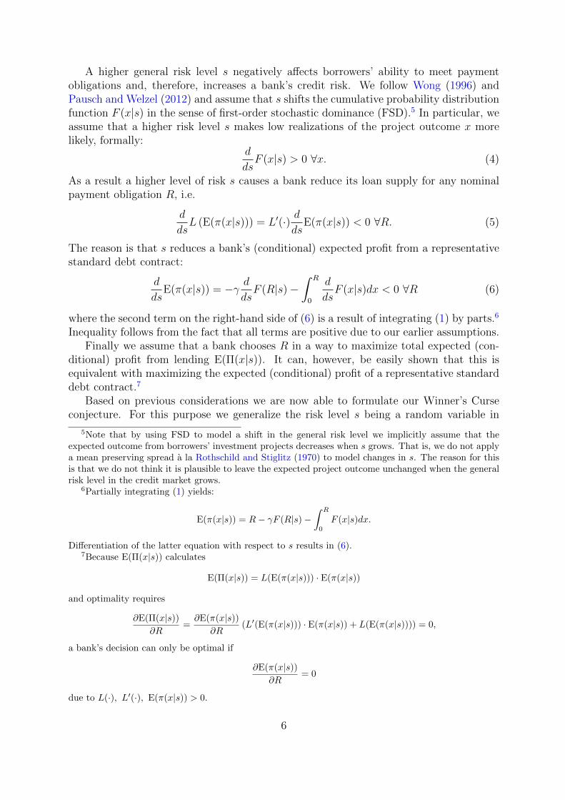
A higher general risk level s negatively affects borrowers’ ability to meet paymentobligations and, therefore, increases a bank’s credit risk. We follow Wong (1996) andPausch and Welzel (2012) and assume that s shifts the cumulative probability distributionfunction F (x|s) in the sense of first-order stochastic dominance (FSD).5 In particular, weassume that a higher risk level s makes low realizations of the project outcome x morelikely, formally:

d

dsF (x|s) > 0 ∀x. (4)

As a result a higher level of risk s causes a bank reduce its loan supply for any nominalpayment obligation R, i.e.

d

dsL (E(π(x|s))) = L′(·) d

dsE(π(x|s)) < 0 ∀R. (5)

The reason is that s reduces a bank’s (conditional) expected profit from a representativestandard debt contract:

d

dsE(π(x|s)) = −γ d

dsF (R|s)−

∫ R

0

d

dsF (x|s)dx < 0 ∀R (6)

where the second term on the right-hand side of (6) is a result of integrating (1) by parts.6

Inequality follows from the fact that all terms are positive due to our earlier assumptions.Finally we assume that a bank chooses R in a way to maximize total expected (con-

ditional) profit from lending E(Π(x|s)). It can, however, be easily shown that this isequivalent with maximizing the expected (conditional) profit of a representative standarddebt contract.7

Based on previous considerations we are now able to formulate our Winner’s Curseconjecture. For this purpose we generalize the risk level s being a random variable in

5Note that by using FSD to model a shift in the general risk level we implicitly assume that theexpected outcome from borrowers’ investment projects decreases when s grows. That is, we do not applya mean preserving spread a la Rothschild and Stiglitz (1970) to model changes in s. The reason for thisis that we do not think it is plausible to leave the expected project outcome unchanged when the generalrisk level in the credit market grows.

6Partially integrating (1) yields:

E(π(x|s)) = R− γF (R|s)−∫ R

0

F (x|s)dx.

Differentiation of the latter equation with respect to s results in (6).7Because E(Π(x|s)) calculates

E(Π(x|s)) = L(E(π(x|s))) · E(π(x|s))

and optimality requires

∂E(Π(x|s))∂R

=∂E(π(x|s))

∂R(L′(E(π(x|s))) · E(π(x|s)) + L(E(π(x|s)))) = 0,

a bank’s decision can only be optimal if

∂E(π(x|s))∂R

= 0

due to L(·), L′(·), E(π(x|s)) > 0.

6

the following. In particular we assume, as is common in the auction theory literature,that each individual bank i in the credit market is uncertain about the actual generalrisk level s and observes just a noisy signal si, i.e. a specific realization of the randomvariable s, which is private information to bank i. Consequently, individual signals siare not independent between banks because they come out of a common random processsi = s + εi where s is the actual general risk level and the εi’s represent iid noise termsof individual banks with E(εi) = 0 ∀i.8 As a result, si is an unbiased estimator for theactual s of any individual bank i.

Now our Winner’s Curse argument goes as follows: based on the private signal si,each individual bank i determines the expected conditional profit of a representative loancontract E(x|si) and the corresponding R∗i which ensures bank i a maximum expectedprofit from lending. As a result, depending on the individual signal si each bank observes acorresponding realization of the conditional expected profit E(π(x|s)) of a representativestandard debt contract. Banks which observe very low signals si will hence infer thatlending is highly profitable and any bank with a low signal si will supply more loans thanany other bank observing a higher risk-level signal sj:

9

Li (E(π(x|si))) > Lj (E(π(x|sj))) because E(π(x|si)) > E(π(x|sj)) ∀ si < sj, i 6= j.

Ex post this is, however, bad news for all banks with individual signals below the truerisk level s, i.e. si < s. All these banks overestimate expected profits from lending andsupply more loans than would be optimal at the prevailing nominal loan payment R∗i .Note that for any given R∗i relations (5) and (6) imply

L (E(π(x|s))) < L (E(π(x|si))) because E(π(x|s)) < E(π(x|si)) ∀ si < s at given R∗i .

Figure 1 illustrates the case.In other words, all banks with si < s are too optimistic about the profit opportunities

in the credit market. As a result their loan supply is too high and, ex post, they willfind themselves in a situation where they face write-downs on loans even if their ex-ante decisions seem to credit-ration borrowers in the sense of Stiglitz and Weiss (1981)and Williamson (1987). A Winner’s Curse situation – well known in auction theory –occurs in the credit market.10 Moreover, in highly competitive credit markets the previousarguments emphasize that particularly banks with very low signals si will behave veryaggressive. This might encourage other banks to lower their credit standards and increasethe volume of loans.

8For a similar setting to model banks’ credit decisions depending on private signals on fundamentals,see Aikman et al. (2015).

9Note, this argument compares specific realizations of conditional expected profits E(π(x|si)) that aredriven by realizations of the common random process si = s+ εi.

10Note, one may argue that banks that behave rational should be aware of this effect and therefore willtake this into account when making decisions. However, there are two arguments for why the Winner’sCurse will still prevail. First, because banks are modeled symmetrically, modifying the decision processfor Winner’s Curse will just reduce expectations on E(π(x|si)). Relative expectations among individualbanks, which depend on the individual signals si, do not change, however. Second, it is absolutely rationalfor each individual bank to formulate expectations E(π(x|si)) based on private signals. This is becauseany bank is aware of the fact that due to the random process si is an unbiased estimator of the actualgeneral risk level s.

7

Figure 1: Loan Supply with si < s

R

L(E(p(x|si)))

L(E(p(x|s)))

Ri*

L(E(p(R*|si)))

L(E(p(R*|s)))

3 Institutional background, methodology and data

3.1 Institutional background

The German banking sector comprises three pillars of universal banks: the commercial,savings, and cooperative bank sector with 1,787 institutions and e6,064 billion in totalassets in 2013. The largest pillar, the sector of commercial banks, is highly concentrated,with the four largest banks representing some 62% of total assets in this segment. In sum,all 277 commercial banks represent 46.0% of total assets in the system of universal banks.

The second-largest group, savings banks and their central institutions (DekaBank andnine Landesbanks), comprise banks which are mostly owned by cities, counties or stategovernments. Within this sector, each savings bank is closely linked to its respectivecentral institution (Landesbank, DekaBank) which provides additional banking services(e.g., securities and international banking). The savings bank sector, including DekaBankand Landesbanks, is rather fractionalized, comprising 421 banks in all. In general, savingsbanks are smaller than private banks and are mainly restricted to the area of the city orcounty in which the bank is located. This “regional principle” makes competition betweensavings banks almost impossible. In 2013 the savings bank sector represented 36.9% ofthe total assets of universal banks in Germany.

The third and smallest pillar comprises cooperative banks. This sector is even morefractionalized than the savings bank pillar as cooperative central banks only hold 26.5%of total assets of the sector and, in addition, the number of banks is larger. Like savingsbanks, cooperative banks are also limited to specific geographic areas, enabling themto compete against commercial and savings banks, but restricting competition withinthe cooperative bank pillar. By law, cooperative banks are committed to promotingthe economic interests of their members, which are also the owners of these banks. In2013, the 1,078 cooperative banks in Germany together with the two central cooperativeinstitutions accounted for 17.1% of total assets in the three-pillar system of universalbanks.

8

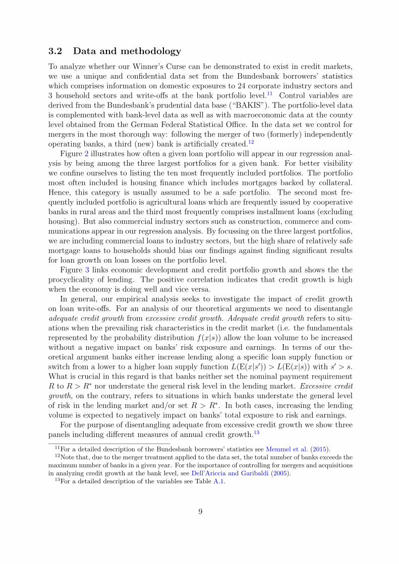
3.2 Data and methodology

To analyze whether our Winner’s Curse can be demonstrated to exist in credit markets,we use a unique and confidential data set from the Bundesbank borrowers’ statisticswhich comprises information on domestic exposures to 24 corporate industry sectors and3 household sectors and write-offs at the bank portfolio level.11 Control variables arederived from the Bundesbank’s prudential data base (“BAKIS”). The portfolio-level datais complemented with bank-level data as well as with macroeconomic data at the countylevel obtained from the German Federal Statistical Office. In the data set we control formergers in the most thorough way: following the merger of two (formerly) independentlyoperating banks, a third (new) bank is artificially created.12

Figure 2 illustrates how often a given loan portfolio will appear in our regression anal-ysis by being among the three largest portfolios for a given bank. For better visibilitywe confine ourselves to listing the ten most frequently included portfolios. The portfoliomost often included is housing finance which includes mortgages backed by collateral.Hence, this category is usually assumed to be a safe portfolio. The second most fre-quently included portfolio is agricultural loans which are frequently issued by cooperativebanks in rural areas and the third most frequently comprises installment loans (excludinghousing). But also commercial industry sectors such as construction, commerce and com-munications appear in our regression analysis. By focussing on the three largest portfolios,we are including commercial loans to industry sectors, but the high share of relatively safemortgage loans to households should bias our findings against finding significant resultsfor loan growth on loan losses on the portfolio level.

Figure 3 links economic development and credit portfolio growth and shows the theprocyclicality of lending. The positive correlation indicates that credit growth is highwhen the economy is doing well and vice versa.

In general, our empirical analysis seeks to investigate the impact of credit growthon loan write-offs. For an analysis of our theoretical arguments we need to disentangleadequate credit growth from excessive credit growth. Adequate credit growth refers to situ-ations when the prevailing risk characteristics in the credit market (i.e. the fundamentalsrepresented by the probability distribution f(x|s)) allow the loan volume to be increasedwithout a negative impact on banks’ risk exposure and earnings. In terms of our the-oretical argument banks either increase lending along a specific loan supply function orswitch from a lower to a higher loan supply function L(E(x|s′)) > L(E(x|s)) with s′ > s.What is crucial in this regard is that banks neither set the nominal payment requirementR to R > R∗ nor understate the general risk level in the lending market. Excessive creditgrowth, on the contrary, refers to situations in which banks understate the general levelof risk in the lending market and/or set R > R∗. In both cases, increasing the lendingvolume is expected to negatively impact on banks’ total exposure to risk and earnings.

For the purpose of disentangling adequate from excessive credit growth we show threepanels including different measures of annual credit growth.13

11For a detailed description of the Bundesbank borrowers’ statistics see Memmel et al. (2015).12Note that, due to the merger treatment applied to the data set, the total number of banks exceeds the

maximum number of banks in a given year. For the importance of controlling for mergers and acquisitionsin analyzing credit growth at the bank level, see Dell’Ariccia and Garibaldi (2005).

13For a detailed description of the variables see Table A.1.

9

Figure 2: Top ten largest domestic credit portfolios

0 1,000 2,000 3,000 4,000 5,000

No. of largest portfolios (bank-year observations) in the sample

Communications; advocacy; publishing; services

Non installment credit without housing finance

Professional housing providers

Other real estate

Installment credit without housing finance

Housing finance

Agriculture, forestry, fishing

Commerce; maintenance/repair of vehicles

Hospitality industry

Construction industry

Top ten largest domestic credit portfolios

• Panel A: CREDIT GROWTH is measured as delta ln credit (if change in credit ispositive)

• Panel B: DUMMY LARGE CREDIT GROWTH takes one when a bank increasesits lending by more than the mean plus two times the standard deviation of thebanking sector.

• Panel C: GAP EXCESSIVE CREDIT GROWTH measures the positive deviationfrom the long-run bank-specific trend in % derived by employing the HP filter.

• Panel D: REL. GAP EXCESSIVE CREDIT GROWTH measures the positivedeviation from the long-run banking sector trend in % derived by employing theHP filter.

Our first measure, CREDIT GROWTH, is simply the change in the log of credit and isset to zero if a bank reports a decline in lending. DUMMY LARGE CREDIT GROWTHis an indicator of extreme lending growth and assigns a value of one to banks that increasetheir lending more than two standard deviations above the mean of their banking sector.Growth rates were separately measured for private commercial, savings, and cooperativebanks. This measure is only assigned to less than five percent of the banks with thehighest credit growth. Nevertheless, our analysis will show that large loan growth does

10

Figure 3: Credit growth and the real economy

-6-4

-20

24

Per

cent

age

chan

ge o

fre

al G

DP

(in

per

cent

)

-10

12

3

Mea

n cr

edit

grow

th(in

per

cent

)

2003 2004 2005 2006 2007 2008 2009 2010 2011 2012 2013

Mean credit growth

Percentage change of real GDP

Credit growth vs. GDP growth

not necessarily mean excessive credit growth. Even the opposite might hold: a bankassigned a value of zero might have excessive credit growth if it is undercapitalized orits loan monitoring techniques are inadequate. Excessive credit growth is calculated asthe deviation from the long-run trend when applying the the HP filter. Using quarterlydata, the smoothing parameter is set to 1,600. Based on credit data from the first quar-ter of 1999 until the end of 2013 we calculate GAP EXCESSIVE CREDIT GROWTHas the percentage of positive deviation from the bank-individual trend and REL. GAPEXCESSIVE CREDIT GROWTH as the percentage positive deviation from the industrytrend,14 i.e. the aggregated growth trend in the banking sector of private commercial,savings or cooperative banks. Excessive growth rates are calculated for total domesticlending as well as the three largest domestic sectoral portfolios. For banks experiencingcredit growth below their long-run trend, GAP EXCESSIVE CREDIT GROWTH is setto zero. We exclude banks and bank portfolios which do not exist for at least ten suc-cessive quarters in the sample period. Following Mendoza and Terrones (2008, 2012), weemploy the standard form of the HP filter and do not use an expanding HP filter as thestandard version proved to be superior in identifying the timing of credit booms. Theirapproach also proved to be suitable for separating the development of bank-level variables— such as profitability, non-performing loans, loan expansion and capital adequacy —of a country’s median bank into boom and bust phases. As the HP filter estimates thecyclical and trend components inaccurately at endpoints (Mise et al., 2005) the standardversion is preferable. Moreover, using previous year-end lagged values of (REL.) GAPEXCESSIVE CREDIT GROWTH excludes the last four less accurately estimated quar-terly observations of excess credit growth from our analysis. Hence, applying the standard

14This measure is similar to that of Dell’Ariccia and Garibaldi (2005).

11

version of the HP filter seems suitable for measuring and timing excessive credit growthat a micro-prudential bank level that might translate into a macroeconomic credit boom.

Furthermore, we consider a set of control variables which help to validate our results.The most important one is a proxy for pricing or market power — the LERNER INDEX.Adjusting the LERNER INDEX for inefficiencies (see, Koetter et al., 2012) allows us toincorporate the idea that banks might exercise even higher market power than their ob-served profits and costs would suggest but forego some of these profits due to non-optimaland therefore inefficient behavior. A higher LERNER INDEX indicates that banks enjoymore price-setting power in the credit market. Banks are, in turn, able to enforce highernominal payment requirements R in loan contracts. Against the background of our the-oretical considerations the LERNER INDEX helps to analyze whether banks operate tothe left or to the right of the optimal R∗ on a given loan supply function. Operating onthe left would result in a negative coefficient and is consistent with the franchise valuetheory of competition (e.g., Keeley, 1990), i.e. that lower competition decreases the riskof default as banks limit risk-taking in order not to lose the franchise value of their op-erations. On the other hand, if we observe a positive impact of the LERNER INDEX onloan losses, a bank would operate to the right of the optimal R∗. This is in line with therisk-shifting hypothesis of competition developed by Boyd and De Nicolo (2005) whichis based on moral hazard behavior of borrowers similar to that modeled in Stiglitz andWeiss (1981). If banks use their price-setting power to increase the nominal repaymentobligation R close to borrowers’ maximum ability to repay, the corresponding increasein the probability of borrowers defaulting on loan repayment would outweigh the posi-tive margin effect of higher loan repayment. By allowing for imperfectly correlated loandefaults, Martinez-Miera and Repullo (2010) demonstrate the existence of a U-shapedrelationship between competition and bank failure. For low levels of competition the risk-shifting effect dominates and an increase in competition reduces bank failure, whereasin markets with a high degree of competition the margin effect of higher interest incomeon performing loans dominates and a further increase in competition makes bank failuremore likely. These non-linearities can be captured empirically by including a squared termof the Lerner index (SQUARED LERNER INDEX) (Jimenez et al., 2013). We expectLERNER INDEX to show a negative coefficient, i.e. higher market power allows banksto choose high-quality borrowers and reduces their charge-off rates. For the SQUAREDterm we expect a positive coefficient as banks that try to extract excessively high ratesfrom their borrowers will observe moral hazard.

Our regression framework has the following form and includes a set of further controlvariables:

LWO = f (CG,BS,C,ME, u) , (7)

where LWO is a vector of loan write-offs. In each panel we compare two model speci-fications: (1) an ordinary least squares (OLS) model with the deviation of loss rate tooverall loss rate (at the bank or the bank-portfolio level for domestic loans), and (2) aTobit model with the loss rate (i.e., the total write-offs to total credit in the domesticcredit portfolio) as the dependent variable. In order to separate the effect of the totaldomestic loan portfolio from the effect of a bank’s three largest portfolios we estimatemodels for both “Total domestic credit” and the “Three largest portfolios of domesticcredit”. All regressions are run for the whole banking system as well as separately for theprivate, savings and cooperative banking pillars. Loan write-offs are a function of a vec-

12

tor CG of three lagged values of the credit growth proxies introduced above. We includelagged values to mitigate endogeneity concerns and control for the fact that borrowersdo not necessarily default in the first year. Instead, contemporaneous write-offs can bethe consequence of credit supply dating back several years. Taking lagged values of upto three periods is supported by other empirical studies (e.g., Foos et al., 2010; Jimenezet al., 2014a). BS is a vector of bank-specific control variables, C is a vector that cap-tures the stance of credit market competition, and ME controls for the macroeconomicenvironment. Bank-specific control variables include EQUITY CAPITAL RATIO, theratio of Tier 1 capital to risk-weighted assets (RWA). Equity serves as a measure of abank’s risk-aversion but also controls for a bank’s ability to lend. CUSTOMER LOANSRATIO is the percentage of customer loans to total assets and controls for the fact thatloans to households and corporates have on average higher default rates. SHARE FEEINCOME is the percentage of fee and commission income to total income and is a proxyfor a bank’s engagement in other than the traditional banking activities. Finally, LOANPORTFOLIO HHI is the Herfindahl-Hirschman Index (HHI) calculated over 8 groupedcredit sectors. Competition C includes the LERNER INDEX and its SQUARED term.ME includes REGIONAL GDP at the county level. All other macroeconomic develop-ments at the national level are captured using YEAR DUMMIES. To control for othertime-invariant regional characteristics, we include STATE DUMMIES. Regional dummiesattempt to capture differing loan demand driving loan losses.15 Finally, u represents theerror term.

From a micro-prudential perspective we want to know whether excessive loan growthmakes banks more risky. Therefore, we replace LWO in further regressions at the banklevel by the ZSCORE, interpreted as a bank’s distance to default. If excessive lendingincreases bank risk, we would expect a negative coefficient on lagged loan growth, i.e. wewould observe a shrinking distance to default. Moreover, we investigate whether excessivelenders are more likely to need capital support (DISTRESS) or to go into outright default(DEFAULT). The latter two regressions are run as probit models and we expect a positivecoefficient on lagged loan growth. In order to address unobserved bank characteristics inour regressions, in evaluating the significance of the results, we report standard errorsclustered on the bank level.

Table 1 presents summary statistics of these variables for the sample between 1999and 2013. The average loss rate for total lending is 0.461%, and slightly higher for thelargest loan portfolio at 0.693%. Annual loan growth for total credit is around 3%, butsignificantly higher for the largest portfolio at around 9%. Hence, banks are more likely toincrease lending to those industry sectors they already have a large experience in. Usingour DUMMY LARGE CREDIT GROWTH, we find that between 3% and 4% of banksshow credit growth in excess of average growth + two standard deviations. Both GAPand REL. GAP EXCESSIVE CREDIT GROWTH are on average around 1% for totalcredit and 4% for the largest portfolio.

15Carlson et al. (2013) find that dummies for metropolitan statistical areas adequately capture localloan demand. The importance to control for local conditions in order to separate supply from demandfactors when investigating loan losses has been stressed by Mian and Sufi (2009). For robustness wereplace the (16) STATE DUMMIES with (415) COUNTY DUMMIES, or in order to control for time-varying local demand conditions (38) ADMINISTRATIVE DISTRICT DUMMIES and interactions ofADMINISTRATIVE DISTRICT DUMMIES and TIME DUMMIES. Results are qualitatively similarand available upon request.

13

Table 1: Descriptive statistics

This table presents descriptive statistics for regulatory data obtained from the Bundesbank. The sample comprises 17,590 bank-year observations for totaldomestic credit and 52,314 bank-year observations to cover the three largest portfolios of domestic credit on up to 2,361 banks reporting during the 1999 –2013 period. LOSS RATE: write-offs (portfolio) to credit (portfolio) in the domestic credit portfolio (three largest domestic credit portfolios); DEVIATIONLOSS RATE (SECTOR): deviation of loss rate (sector) from the industry aggregate (commercial bank sector, public bank sector, cooperative bank sector)per year; DISTRESS: dummy variable that takes on the value of one for banks receiving capital support measures from the deposit insurance funds, orexiting the market in a distressed merger/in a moratorium; DEFAULT: dummy variable that takes on the value of one for banks exiting the market in adistressed merger/in a moratorium; ZSCORE: Ln of the z-score calculated as the ratio of equity capital and operating profits to the standard deviation ofoperating profits (all components scaled by total assets). CREDIT GROWTH is defined as delta ln credit for positive changes; DUMMY LARGE CREDITGROWTH is a dummy variable that takes on the value of one when the threshold per banking group (mean growth + 2 standard deviations) is exceeded;GAP EXCESSIVE CREDIT GROWTH is the positive deviation from the long-run trend (measured in %); REL. GAP EXCESSIVE CREDIT GROWTH isthe positive deviation from the long-run trend (measured in %) adjusted by the industry aggregate (i.e. the positive deviation from the long-run trend for thecommercial bank sector, public bank sector, cooperative bank sector); L1 - L3 denote lag-operators. Bank-specific control variables are measured in percent(REGIONAL GDP as a percentage change) and averaged over three years. Note: For ZSCORE regressions the number of observations is 17,024.

Total domestic credit Largest portfolio of domestic credit

Variable Mean SD P10 P25 P50 P75 P90 Mean SD P10 P25 P50 P75 P90

Dependent variables

LOSS RATE 0.461 0.63 0.00 0.07 0.28 0.60 1.09 0.693 1.44 0.00 0.00 0.10 0.73 2.00

DEVIATION LOSS RATE 0.157 0.60 -0.29 -0.18 0.00 0.29 0.74 0.480 1.36 -0.28 -0.09 0.00 0.49 1.68

DISTRESS 0.014 0.12 0.00 0.00 0.00 0.00 0.00

DEFAULT 0.005 0.07 0.00 0.00 0.00 0.00 0.00

ZSCORE 3.166 0.65 2.33 2.74 3.18 3.60 4.01

CREDIT GROWTH

L1.CREDIT GROWTH 2.383 4.10 0.00 0.00 0.64 3.37 6.49 8.910 21.01 0.00 0.00 0.95 9.56 23.23

L2.CREDIT GROWTH 2.373 4.32 0.00 0.00 0.54 3.27 6.41 8.809 20.76 0.00 0.00 0.61 9.33 23.46

L3.CREDIT GROWTH 3.248 6.14 0.00 0.00 0.82 4.05 8.35 9.606 22.11 0.00 0.00 1.11 10.33 25.79

DUMMY LARGE CREDIT GROWTH (threshold per banking group: mean growth + 2 standard deviations)

L1.DUMMY LARGE CG 0.033 0.18 0.00 0.00 0.00 0.00 0.00 0.036 0.19 0.00 0.00 0.00 0.00 0.00

L2.DUMMY LARGE CG 0.034 0.18 0.00 0.00 0.00 0.00 0.00 0.036 0.19 0.00 0.00 0.00 0.00 0.00

L3.DUMMY LARGE CG 0.070 0.26 0.00 0.00 0.00 0.00 0.00 0.039 0.19 0.00 0.00 0.00 0.00 0.00

GAP EXCESSIVE CREDIT GROWTH

L1.GAP EXCESSIVE CG 0.832 1.87 0.00 0.00 0.00 1.00 2.39 4.554 8.83 0.00 0.00 0.18 5.23 13.61



RELATIVE GAP EXCESSIVE CREDIT GROWTH (industry adjusted)

L1.REL. GAP EXCESSIVE CG 0.954 1.94 0.00 0.00 0.00 1.25 2.72 4.615 8.39 0.00 0.00 0.47 5.77 13.86



Bank-specific control variables (averaged over three years)

EQUITY CAPITAL RATIO 5.981 2.16 4.10 4.80 5.63 6.64 8.08 5.962 2.19 4.10 4.80 5.63 6.62 8.03

CUSTOMER LOANS RATIO 57.292 14.14 38.25 50.23 59.10 66.51 73.26 57.466 13.87 38.81 50.40 59.16 66.53 73.25

OBS ACTIVITIES 5.544 5.70 2.07 3.07 4.50 6.55 9.48 5.525 5.58 2.08 3.08 4.50 6.54 9.43

SHARE FEE INCOME 13.814 7.24 8.13 10.33 12.82 15.75 19.03 13.726 7.01 8.16 10.34 12.81 15.72 18.92

LOAN PORTFOLIO HHI 13.486 10.58 7.64 8.54 10.22 13.67 21.01 13.169 9.74 7.64 8.53 10.19 13.52 20.34

LERNER INDEX 0.478 0.07 0.41 0.45 0.48 0.52 0.55 0.478 0.08 0.41 0.45 0.48 0.51 0.55

SQUARED LERNER INDEX 0.235 0.07 0.17 0.20 0.23 0.27 0.30 0.236 0.16 0.17 0.20 0.23 0.27 0.30

PERSONNEL INTENSITY 0.371 0.58 0.21 0.27 0.33 0.41 0.54 0.368 0.42 0.21 0.27 0.33 0.41 0.54

Macroeconomic control variable

REGIONAL GDP 1.247 1.90 -1.01 0.02 1.15 2.40 3.51 1.252 1.90 -1.01 0.02 1.16 2.41 3.52

Banking group dummies

DUMMY SAVINGS BANKS 0.263 0.44 0.00 0.00 0.00 1.00 1.00 0.265 0.44 0.00 0.00 0.00 1.00 1.00

DUMMY COOP. BANKS 0.663 0.47 0.00 0.00 1.00 1.00 1.00 0.667 0.47 0.00 0.00 1.00 1.00 1.00

Observations 17,590 52,314

14

Tab

le2:

Cor

rela

tion

mat

rice

s

Th

ista

ble

pre

sents

resu

lts

from

poole

dP

rob

itre

gre

ssio

ns

wit

hD

IST

RE

SS

:a

du

mm

yvari

ab

leth

at

takes

on

the

valu

eof

on

efo

rb

an

ks

rece

ivin

gca

pit

al

sup

port

mea

sure

sfr

om

the

dep

osi

tin

sura

nce

fun

ds,

or

exit

ing

the

mark

etin

ad

istr

esse

dm

erger

/in

am

ora

tori

um

/D

EFA

ULT

:a

du

mm

yvari

ab

leth

at

takes

on

the

valu

eof

on

efo

rb

an

ks

exit

ing

the

mark

etin

ad

istr

esse

dm

erger

/in

am

ora

tori

um

as

the

dep

end

ent

vari

ab

le;

more

over

,p

oole

dO

LS

regre

ssio

ns

wit

hZ

SC

OR

E:

the

lnof

the

z-sc

ore

calc

ula

ted

as

the

rati

oof

equ

ity

cap

ital

an

dop

erati

ng

pro

fits

toth

est

an

dard

dev

iati

on

of

op

erati

ng

pro

fits

(all

com

pon

ents

scale

dby

tota

lass

ets)

as

the

dep

end

ent

vari

ab

leare

show

n.

CR

ED

ITG

RO

WT

His

defi

ned

as

del

taln

cred

itfo

rp

osi

tive

chan

ges

;D

UM

MY

LA

RG

EC

RE

DIT

GR

OW

TH

isa

du

mm

yvari

ab

leth

at

takes

on

the

valu

eof

on

ew

hen

the

thre

shold

per

ban

kin

ggro

up

(mea

ngro

wth

+2

stan

dard

dev

iati

on

s)is

exce

eded

;G

AP

EX

CE

SS

IVE

CR

ED

ITG

RO

WT

His

the

posi

tive

dev

iati

on

from

the

lon

g-r

un

tren

d(m

easu

red

in%

);R

EL

.G

AP

EX

CE

SS

IVE

CR

ED

ITG

RO

WT

His

the

posi

tive

dev

iati

on

from

the

lon

g-r

un

tren

d(m

easu

red

in%

)ad

just

edby

the

ind

ust

ryaggre

gate

(i.e

.th

ep

osi

tive

dev

iati

on

from

the

lon

g-r

un

tren

dfo

rth

eco

mm

erci

al

ban

kse

ctor,

pu

blic

ban

kse

ctor,

coop

erati

ve

ban

kse

ctor)

;L

1-

L3

den

ote

lag-o

per

ato

rs;

Ba

nk-

spec

ific

con

tro

lva

ria

bles

are

mea

sure

din

per

cent

(RE

GIO

NA

LG

DP

as

ap

erce

nta

ge

chan

ge)

an

daver

aged

over

thre

eyea

rs.

***

p<

0.0

1,

**

p<

0.0

5,

*p<

0.1

;st

an

dard

erro

rscl

ust

ered

at

ban

kle

vel

(ban

k-p

ort

folio

level

)in

pare

nth

eses

.

(1)

(2)

(3)

(4)

(5)

(6)

(7)

(8)

(9)

(10)

(11)

(12)

(13)

(14)

(15)

(16)

(17)

(18)

(19)

(20)

(21)

(22)

(23)

(24)

(25)

(26)

(27)

(28)

(1)

LO

SS

RA

TE

1.0

00

(2)

DE

VIA

TIO

NL

OSS

RA

TE

0.9

83

1.0

00

(3)

DIS

TR

ESS

0.1

23

0.1

24

1.0

00

(4)

DE

FA

ULT

0.0

90

0.0

93

0.1

98

1.0

00

(5)

ZSC

OR

E-0

.197

-0.2

16

-0.1

06

-0.0

88

1.0

00

(6)

L1.C

RE

DIT

GR

OW

TH

-0.0

67

-0.0

91

-0.0

18

-0.0

19

-0.0

24

1.0

00

(7)

L2.C

RE

DIT

GR

OW

TH

-0.0

40

-0.0

58

-0.0

07

-0.0

04

-0.0

42

0.5

69

1.0

00

(8)

L3.C

RE

DIT

GR

OW

TH

0.0

39

0.0

44

0.0

27

0.0

16

-0.0

79

0.3

07

0.4

37

1.0

00

(9)

L1.D

UM

MY

LA

RG

EC

G-0

.033

-0.0

40

0.0

00

-0.0

09

-0.0

41

0.6

33

0.3

43

0.1

79

1.0

00

(10)

L2.D

UM

MY

LA

RG

EC

G-0

.018

-0.0

23

0.0

10

0.0

04

-0.0

54

0.3

72

0.6

53

0.2

71

0.3

76

1.0

00

(11)

L3.D

UM

MY

LA

RG

EC

G0.0

35

0.0

48

0.0

26

0.0

18

-0.0

70

0.1

69

0.2

67

0.7

37

0.1

45

0.2

74

1.0

00

(12)

L1.G

AP

EX

CE

SSIV

EC

G0.1

11

0.1

07

0.0

71

0.0

41

-0.1

03

0.4

40

0.4

56

0.2

81

0.2

65

0.2

93

0.1

69

1.0

00

(13)

L2.G

AP

EX

CE

SSIV

EC

G0.1

47

0.1

59

0.0

73

0.0

42

-0.1

33

-0.0

66

0.3

89

0.4

83

-0.0

43

0.2

31

0.3

30

0.3

97

1.0

00

(14)

L3.G

AP

EX

CE

SSIV

EC

G0.1

45

0.1

67

0.0

77

0.0

36

-0.1

31

-0.0

94

-0.0

83

0.5

66

-0.0

36

-0.0

56

0.4

27

0.0

62

0.4

80

1.0

00

(15)

L1.R

EL

.G

AP

EX

CE

SSIV

EC

G0.1

05

0.1

04

0.0

68

0.0

40

-0.0

95

0.4

10

0.4

27

0.2

58

0.2

48

0.2

67

0.1

43

0.9

40

0.3

85

0.0

59

1.0

00

(16)

L2.R

EL

.G

AP

EX

CE

SSIV

EC

G0.1

21

0.1

13

0.0

62

0.0

33

-0.0

97

-0.0

68

0.3

72

0.4

47

-0.0

47

0.2

18

0.2

92

0.3

76

0.9

28

0.4

45

0.4

07

1.0

00

(17)

L3.R

EL

.G

AP

EX

CE

SSIV

EC

G0.1

13

0.1

07

0.0

68

0.0

22

-0.0

95

-0.0

89

-0.0

83

0.5

24

-0.0

39

-0.0

58

0.3

92

0.0

42

0.4

32

0.9

25

0.0

47

0.4

70

1.0

00

(18)

EQ

UIT

YC

AP

ITA

LR

AT

IO-0

.013

-0.0

48

-0.0

59

-0.0

35

0.1

96

0.1

66

0.1

54

0.1

13

0.0

87

0.0

68

0.0

15

0.1

26

0.0

95

0.0

94

0.1

21

0.1

12

0.1

20

1.0

00

(19)

CU

ST

OM

ER

LO

AN

SR

AT

IO-0

.007

0.0

04

-0.0

12

-0.0

08

0.1

27

-0.0

42

-0.0

04

0.0

08

-0.0

64

-0.0

39

-0.0

02

-0.0

71

-0.0

62

-0.0

80

-0.0

49

-0.0

54

-0.0

89

-0.0

03

1.0

00

(20)

OB

SA

CT

IVIT

IES

0.0

36

0.0

35

0.0

00

-0.0

01

-0.0

39

0.1

15

0.1

16

0.0

94

0.0

78

0.0

91

0.0

51

0.0

97

0.1

09

0.0

94

0.0

80

0.0

92

0.0

82

0.0

52

0.1

04

1.0

00

(21)

SH

AR

EF

EE

INC

OM

E0.0

42

-0.0

04

0.0

05

0.0

06

-0.0

80

0.1

76

0.1

69

0.1

32

0.0

83

0.0

69

0.0

30

0.1

59

0.1

35

0.1

17

0.1

36

0.1

50

0.1

53

0.2

86

-0.2

85

0.0

77

1.0

00

(22)

LO

AN

PO

RT

FO

LIO

HH

I-0

.013

-0.0

11

0.0

03

0.0

17

-0.0

62

0.3

14

0.3

33

0.2

79

0.1

81

0.1

91

0.1

24

0.2

44

0.2

45

0.2

05

0.2

37

0.2

29

0.1

82

0.2

93

-0.1

42

0.0

87

0.1

80

1.0

00

(23)

LE

RN

ER

IND

EX

-0.0

33

-0.0

91

-0.0

94

-0.0

44

0.2

39

0.0

18

0.0

16

-0.0

37

-0.0

29

-0.0

22

-0.0

47

-0.0

20

-0.0

70

-0.0

91

-0.0

34

-0.0

38

-0.0

46

0.3

19

0.0

45

0.0

41

0.1

13

-0.0

21

1.0

00

(24)

SQ

UA

RE

DL

ER

NE

RIN

DE

X-0

.011

-0.0

61

-0.0

72

-0.0

41

0.1

59

0.0

98

0.0

70

0.0

08

0.0

40

0.0

24

-0.0

17

0.0

13

-0.0

38

-0.0

64

-0.0

01

-0.0

12

-0.0

25

0.3

29

-0.0

17

0.0

37

0.1

68

0.0

49

0.5

31

1.0

00

(25)

PE

RSO

NN

EL

INT

EN

SIT

Y0.0

06

0.0

12

0.0

05

0.0

08

-0.0

43

0.0

21

0.0

30

0.0

34

0.0

13

0.0

02

0.0

08

0.0

61

0.1

02

0.1

19

0.0

58

0.0

85

0.1

02

0.2

09

-0.1

95

-0.0

65

0.2

82

0.0

96

-0.0

50

0.0

50

1.0

00

(26)

RE

GIO

NA

LG

DP

0.0

07

-0.0

24

-0.0

02

0.0

10

0.0

39

-0.0

22

-0.0

16

-0.0

08

-0.0

29

-0.0

24

-0.0

14

0.0

13

-0.0

21

-0.0

42

-0.0

19

0.0

04

0.0

01

0.0

00

-0.0

33

-0.0

27

0.0

30

-0.0

38

0.0

33

0.0

23

0.0

10

1.0

00

(27)

DU

MM

YSA

VIN

GS

BA

NK

S-0

.007

0.0

76

-0.0

22

-0.0

19

-0.0

34

-0.1

65

-0.1

48

-0.1

39

-0.0

37

-0.0

29

-0.0

24

-0.0

87

-0.0

97

-0.1

19

-0.0

96

-0.1

13

-0.1

25

-0.2

66

0.0

42

-0.0

30

-0.2

11

-0.2

38

-0.1

06

-0.1

20

-0.0

70

0.0

06

1.0

00

(28)

DU

MM

YC

OO

P.

BA

NK

S-0

.050

-0.1

24

0.0

09

0.0

13

0.1

07

-0.0

30

-0.0

63

-0.0

32

-0.0

36

-0.0

52

-0.0

20

-0.1

13

-0.0

99

-0.0

36

-0.0

99

-0.0

80

-0.0

29

0.0

81

0.0

49

-0.0

62

-0.0

30

-0.0

53

0.1

39

0.0

99

0.0

10

0.0

23

-0.8

38

1.0

00

15

4 Results

4.1 Adequate credit growth

As shown in Tables 3 for OLS and 4 for Tobit models, analyzing the effect of CREDITGROWTH in general, i.e. without making corrections for certain thresholds or the long-term trend, does not support our Winner’s Curse conjecture and we observe significantlynegative or insignificant coefficients on lagged CREDIT GROWTH. This suggests thatin general, increasing the loan volume reduces banks’ loan write-offs, and loan growthis adequate. Coefficients for the three largest portfolios are less pronounced than fortotal domestic credit, but increasing the number of observations by almost three timesimproves statistical significance. Results are robust to different kind of estimations (OLSvs. Tobit).16

Taking a look at the control variables, we find that a higher CUSTOMER LOANSRATIO increases loan write-offs. This is consistent with loans to households and corpo-rates being on average riskier than those to financial institutions. For small, local banks(i.e. savings and cooperative banks) we find support for the model of Martinez-Mieraand Repullo (2010). We find that a higher LERNER INDEX decreases loan defaults but,as the SQUARED term is positive, the relationship changes for high levels of LERNERINDEX. For savings and cooperative banks higher market power increases loan defaults ata level of 0.88. Hence, only banks that try to exploit very high margins with a LERNERINDEX more than five standard deviations above the mean (mean: 0.48; std: 0.07) willexperience situations in which the risk-shifting channel dominates the margin channel.At the portfolio level this result only holds for cooperative banks and for the total sam-ple, whereas for savings banks the SQUARED term becomes insignificant. Consequently,banks appear to be able to exploit price-setting power in order to stabilize earnings fromlending, and only those banks that charge excessively high rates suffer disproportionatelylarge losses. The coefficients OBS ACTIVITIES and PERSONNEL INTENSITY remaininsignificant.

The previous results basically hold even when we consider a relatively high thresh-old of two standard deviations above the mean growth rate for a banking sector. Twoobservations are, however, noteworthy: on the one hand, the coefficients of the controlvariables appear robust in terms of sign, magnitude and significance. On the other hand,although the signs of the DUMMY LARGE CREDIT GROWTH coefficients are basicallythe same as those for positive credit growth above, significance appears weaker. The F-statistics of joint significance of the coefficients still indicate significantly negative effectsbut are lower in magnitude than the corresponding F-statistics for CREDIT GROWTH.The latter observations, therefore, indicate that results may change when credit growthbecomes extraordinarily large (see Tables 5 and 6).

In contrast, previous studies found significant effects of lagged (abnormal) loan growthmeasures on loan losses. Salas and Saurina (2002) and Jimenez and Saurina (2006) findthat even lagged normal loan growth has a positive impact on non-performing loans.Foos et al. (2010) find that their lags of abnormal loan growth — defined as the differ-ence of bank-specific to a country’s aggregate loan growth — is positive and statisticallysignificant.

16For robustness, we replace CREDIT GROWTH, for which loan contraction has been set to zero witha variable that allows for negative loan growth. Results are robust and lagged loan growth has an evenlarger positive impact. 16

Table 3: Panel A1. Pooled OLS model with CREDIT GROWTH

This table presents results from pooled OLS regressions with DEVIATION LOSS RATE (SECTOR): deviation of loss rate (sector) from the industryaggregate (commercial bank sector, public bank sector, cooperative bank sector) per year as the dependent variable; CREDIT GROWTH is definedas delta ln credit for positive changes; L1 - L3 denote lag-operators; Bank-specific control variables are measured in percent (REGIONAL GDP as apercentage change) and averaged over three years. *** p<0.01, ** p<0.05, * p<0.1; standard errors clustered at bank level (bank-portfolio level) inparentheses.

Total domestic credit Three largest portfolios of domestic credit

Variable All Private Savings Coops All Private Savings Coops

Credit growth

L1.CREDIT GROWTH -0.0105*** -0.0094*** -0.0160** -0.0157*** -0.0018*** -0.0025* -0.0040*** -0.0017***

[-5.9443] [-3.2577] [-2.5632] [-7.3843] [-5.3463] [-1.7753] [-5.6380] [-4.7691]

L2.CREDIT GROWTH -0.0060*** -0.0094*** -0.0087* -0.0029 -0.0011*** -0.0011 -0.0023*** -0.0009***

[-3.2949] [-3.4186] [-1.6664] [-1.4499] [-3.9894] [-0.7858] [-4.0348] [-3.3870]

L3.CREDIT GROWTH 0.0030** 0.0025 -0.0004 0.0022 -0.0007*** -0.0014* -0.0002 -0.0008***

[2.1270] [0.8568] [-0.1182] [1.5904] [-2.9390] [-1.9618] [-0.2469] [-3.3049]


EQUITY CAPITAL RATIO 0.0018 0.0120 -0.0443*** -0.0127 -0.0147** 0.0000 -0.0803*** -0.0381***

[0.2556] [1.2813] [-2.9621] [-1.2697] [-2.4516] [0.0022] [-4.3627] [-4.5382]

CUSTOMER LOANS RATIO 0.0032*** 0.0042** 0.0049** 0.0015* 0.0050*** 0.0057*** 0.0094*** 0.0021**

[3.8652] [2.1051] [2.4486] [1.9340] [6.0884] [3.3403] [4.2559] [2.1464]

OBS ACTIVITIES 0.0024 -0.0014 0.0030 0.0121* -0.0003 -0.0012 -0.0031 -0.0003

[1.0663] [-0.6499] [0.6493] [1.8762] [-0.2131] [-0.7436] [-0.5838] [-0.0634]

SHARE FEE INCOME 0.0007 0.0006 -0.0208** 0.0002 -0.0008 0.0004 -0.0186* 0.0006

[0.3723] [0.2134] [-2.2746] [0.0629] [-0.5037] [0.1627] [-1.8537] [0.2016]

LOAN PORTFOLIO HHI -0.0050*** -0.0011 -0.0058 -0.0092*** -0.0047*** 0.0004 -0.0170** -0.0105***

[-2.9182] [-0.4990] [-0.7258] [-2.9883] [-3.2795] [0.1674] [-2.2191] [-5.3532]

LERNER INDEX -0.1643 -0.0078 -5.2876** -3.1018*** -0.5247** -0.2343 -4.8329 -5.1450***

[-0.4015] [-0.0281] [-2.0767] [-8.0958] [-2.0873] [-0.8946] [-1.5918] [-6.2237]

SQUARED LERNER INDEX 0.1759 -0.1645 6.0162** 3.5352*** -0.0588 -0.0957 4.9792 5.1910***

[0.5276] [-1.2102] [2.1598] [9.1311] [-1.2880] [-1.2676] [1.5109] [5.7865]

PERSONNEL INTENSITY -0.0151 -0.0190 0.3285 -0.1273 -0.0294 -0.0089 0.8298** -0.4569***

[-1.3160] [-1.3744] [1.1524] [-1.4730] [-1.2105] [-0.4560] [2.4066] [-4.6955]

Macroeconomic control variables

REGIONAL GDP 0.0049 0.0302 0.0096 0.0007 0.0005 0.0108 0.0115 -0.0069

[1.3542] [1.1996] [1.4742] [0.1938] [0.1230] [0.3868] [1.4234] [-1.4124]

STATE/YEAR DUMMIES YES YES

Banking group dummies and constant

DUMMY SAVINGS BANKS -0.4390*** -0.3871***

[-6.1001] [-6.9579]

DUMMY COOP. BANKS -0.3868*** -0.2938***

[-5.8363] [-5.5937]

Constant 0.4335** 0.4091 1.4673*** 1.1079*** 1.4080*** 0.5583** 1.5455** 2.2021***

[2.5764] [1.5004] [2.6505] [5.6157] [11.5283] [2.2785] [2.2434] [9.4927]

Observations 17,590 1,302 4,621 11,667 52,314 3,538 13,863 34,913

Number of banks / portfolios 2,361 184 571 1,607 10,706 818 2,660 7,231

Adjusted R-squared 0.088 0.065 0.147 0.102 0.040 0.033 0.074 0.051

L1-3.CREDIT GROWTH (F stat) 20.553 8.815 3.845 23.481 19.891 3.027 15.436 15.211

L1-3.CREDIT GROWTH (p value) 0.000 0.000 0.010 0.000 0.000 0.029 0.000 0.000

17

Table 4: Panel A2. Pooled Tobit model with CREDIT GROWTH

This table presents results from pooled Tobit regressions with LOSS RATE: write-offs (portfolio) to credit (portfolio) in the domestic credit portfolioas the dependent variable; CREDIT GROWTH is defined as delta ln credit for positive changes; L1 - L3 denote lag-operators; Bank-specific controlvariables are measured in percent (REGIONAL GDP as a percentage change) and averaged over three years. *** p<0.01, ** p<0.05, * p<0.1; standarderrors clustered at bank level (bank-portfolio level) in parentheses.



Credit growth

L1.CREDIT GROWTH -0.0130*** -0.0150*** -0.0169*** -0.0185*** -0.0026*** -0.0064*** -0.0047*** -0.0022***

[-5.8323] [-3.2678] [-2.5890] [-6.8008] [-4.4963] [-8.4181] [-4.8412] [-3.6935]

L2.CREDIT GROWTH -0.0083*** -0.0131*** -0.0087 -0.0059** -0.0013*** -0.0029*** -0.0019** -0.0009*

[-3.7045] [-3.1839] [-1.5987] [-2.4360] [-2.7022] [-3.5407] [-2.3838] [-1.8428]

L3.CREDIT GROWTH 0.0026 -0.0001 -0.0007 0.0024 -0.0008* -0.0038*** -0.0003 -0.0004

[1.5715] [-0.0219] [-0.1859] [1.5787] [-1.9288] [-5.2849] [-0.3364] [-0.8168]


EQUITY CAPITAL RATIO -0.0033 0.0182 -0.0442*** -0.0268** -0.0659*** -0.0170*** -0.0716*** -0.1375***

[-0.3491] [1.1877] [-2.8180] [-2.0040] [-4.3809] [-2.9330] [-2.9112] [-6.8199]

CUSTOMER LOANS RATIO 0.0047*** 0.0111*** 0.0050** 0.0016 0.0120*** 0.0282*** 0.0103*** 0.0024

[4.5162] [3.5970] [2.4347] [1.4639] [7.8139] [31.9429] [3.6036] [1.1312]

OBS ACTIVITIES 0.0033 -0.0034 0.0034 0.0152* 0.0031 0.0012 0.0020 0.0067

[1.0901] [-0.7438] [0.6960] [1.8737] [0.8078] [0.7802] [0.2970] [0.7709]

SHARE FEE INCOME 0.0006 0.0002 -0.0220** 0.0007 0.0033 -0.0038** -0.0249* 0.0166**

[0.2400] [0.0343] [-2.2838] [0.1933] [0.8538] [-2.2973] [-1.9222] [2.4755]

LOAN PORTFOLIO HHI -0.0081*** -0.0055 -0.0055 -0.0139*** -0.0195*** -0.0107*** -0.0184* -0.0342***

[-3.4590] [-1.5356] [-0.6718] [-3.0165] [-6.1980] [-7.6197] [-1.6989] [-5.8826]

LERNER INDEX -0.1811 0.6729 -4.9583* -3.3497*** -1.2266*** 0.5370*** 0.8992 -6.1180***

[-0.3672] [0.5012] [-1.8331] [-8.1010] [-2.6283] [3.8227] [0.2212] [-7.5555]

SQUARED LERNER INDEX 0.2099 -0.9442 5.6265* 3.8092*** 0.0816 -1.7392*** -2.1498 5.5685***

[0.5451] [-0.5500] [1.9071] [8.6413] [0.5072] [-6.9808] [-0.4897] [5.9033]

PERSONNEL INTENSITY -0.0368 -0.0489 0.3649 -0.2405** -0.4734** -0.0926*** 0.5726 -1.3798***

[-0.7565] [-1.3267] [1.2442] [-2.0067] [-2.4678] [-2.8334] [1.3396] [-4.7430]


REGIONAL GDP 0.0047 0.0451 0.0091 0.0003 -0.0071 0.0267** 0.0046 -0.0159*

[1.1313] [1.5883] [1.3300] [0.0593] [-1.0440] [2.3189] [0.4372] [-1.9408]


INDUSTRY SECTOR DUMMIES NO YES

Banking group dummies, and constant

DUMMY SAVINGS BANKS -0.3657*** -0.1301

[-4.1645] [-1.3389]

DUMMY COOP. BANKS -0.4687*** -0.5419***

[-5.7898] [-5.8582]

Constant 0.6114*** -0.2395 1.5468*** 1.2273*** 0.4416 -16.3037*** 0.3728 2.1565***

[2.8496] [-0.4979] [2.6617] [4.6084] [1.0599] [-238.9051] [0.4065] [4.1017]

Observations 17,590 1,302 4,621 11,667 52,314 3,538 13,863 34,913


Pseudo R-squared 0.070 0.066 0.115 0.080 0.045 0.064 0.042 0.047

L1-3.CREDIT GROWTH (F stat) 20.565 7.683 3.815 20.340 9.214 367.670 9.079 5.046

L1-3.CREDIT GROWTH (p value) 0.000 0.000 0.010 0.000 0.000 0.000 0.000 0.002

18

Table 5: Panel B1. Pooled OLS model with DUMMY LARGE CREDIT GROWTH(mean + 2 Std)

This table presents results from pooled OLS regressions with DEVIATION LOSS RATE (SECTOR): deviation of loss rate (sector) from the industryaggregate (commercial bank sector, public bank sector, cooperative bank sector) per year as the dependent variable; DUMMY LARGE CREDIT GROWTHis a dummy variable that takes on the value of one when the threshold per banking group (mean growth + 2 standard deviations) is exceeded; L1 - L3denote lag-operators; Bank-specific control variables are measured in percent (REGIONAL GDP as a percentage change) and averaged over three years.*** p<0.01, ** p<0.05, * p<0.1; standard errors clustered at bank level (bank-portfolio level) in parentheses.




L1.DUMMY LARGE CG -0.0877*** -0.2272*** -0.1020* -0.0947*** -0.1150*** -0.2299** -0.1756*** -0.1087***

[-3.2588] [-2.8874] [-1.7942] [-3.7006] [-4.1395] [-2.1638] [-3.3632] [-3.1849]

L2.DUMMY LARGE CG -0.0528 -0.2663*** -0.0685 0.0011 -0.0799*** -0.1356 -0.1230*** -0.0692**

[-1.6306] [-3.4939] [-1.1136] [0.0346] [-3.1093] [-1.1842] [-3.0274] [-2.1897]

L3.DUMMY LARGE CG 0.0445* 0.0198 0.0137 0.0440* -0.0643** -0.1509* -0.0634 -0.0770**

[1.7313] [0.1996] [0.2299] [1.7313] [-2.3077] [-1.6936] [-1.2694] [-2.4077]


EQUITY CAPITAL RATIO 0.0024 0.0134 -0.0400*** -0.0093 -0.0149** -0.0003 -0.0789*** -0.0382***

[0.3338] [1.3828] [-2.6456] [-0.9047] [-2.4911] [-0.0477] [-4.2845] [-4.5351]

CUSTOMER LOANS RATIO 0.0030*** 0.0033* 0.0048** 0.0013* 0.0050*** 0.0056*** 0.0095*** 0.0020**

[3.5631] [1.7007] [2.4570] [1.6515] [6.0132] [3.2756] [4.3083] [2.0543]

OBS ACTIVITIES 0.0021 -0.0011 0.0021 0.0099 -0.0004 -0.0012 -0.0034 -0.0005

[0.9517] [-0.5283] [0.4382] [1.5504] [-0.2817] [-0.7301] [-0.6306] [-0.1250]

SHARE FEE INCOME 0.0007 0.0006 -0.0219** 0.0017 -0.0008 0.0003 -0.0194* 0.0011

[0.3759] [0.2231] [-2.4053] [0.6281] [-0.4916] [0.1237] [-1.9323] [0.3551]

LOAN PORTFOLIO HHI -0.0058*** -0.0010 -0.0085 -0.0101*** -0.0049*** 0.0003 -0.0180** -0.0106***

[-3.4145] [-0.4609] [-1.0983] [-3.2623] [-3.4550] [0.1093] [-2.3574] [-5.4299]

LERNER INDEX -0.1499 -0.0291 -5.1155** -2.9098*** -0.5287** -0.2177 -4.7509 -5.1401***

[-0.3752] [-0.1052] [-1.9874] [-6.8736] [-2.1063] [-0.8291] [-1.5684] [-6.1995]

SQUARED LERNER INDEX 0.1469 -0.1792 5.7221** 3.2480*** -0.0603 -0.0905 4.8623 5.1569***

[0.4532] [-1.3000] [2.0284] [7.8680] [-1.3245] [-1.1923] [1.4786] [5.7320]

PERSONNEL INTENSITY -0.0152 -0.0227 0.3651 -0.1265 -0.0285 -0.0085 0.8691** -0.4574***

[-1.2823] [-1.5991] [1.2705] [-1.4379] [-1.1848] [-0.4361] [2.5077] [-4.6871]


REGIONAL GDP 0.0050 0.0291 0.0090 0.0005 0.0012 0.0115 0.0112 -0.0061

[1.3638] [1.1681] [1.3577] [0.1460] [0.2691] [0.4115] [1.3798] [-1.2487]




[-5.4764] [-6.5405]

DUMMY COOP. BANKS -0.3419*** -0.2761***

[-5.3244] [-5.2726]

Constant 0.4160*** 0.3751 1.3846** 0.8067*** 1.0264*** 0.5130** 1.5008** 2.1805***

[2.6005] [1.3664] [2.4851] [3.7341] [8.5898] [2.0832] [2.1837] [9.3847]

Observations 17,590 1,302 4,621 11,667 52,314 3,538 13,863 34,913



L1-3.DUMMY LARGE CG (F stat) 5.823 6.723 1.485 4.931 10.238 2.447 6.714 7.062

L1-3.DUMMY LARGE CG (p value) 0.001 0.000 0.218 0.002 0.000 0.063 0.000 0.000

19

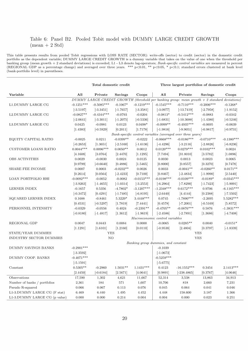
Table 6: Panel B2. Pooled Tobit model with DUMMY LARGE CREDIT GROWTH(mean + 2 Std)

This table presents results from pooled Tobit regressions with LOSS RATE (SECTOR): write-offs (sector) to credit (sector) in the domestic creditportfolio as the dependent variable; DUMMY LARGE CREDIT GROWTH is a dummy variable that takes on the value of one when the threshold perbanking group (mean growth + 2 standard deviations) is exceeded; L1 - L3 denote lag-operators; Bank-specific control variables are measured in percent(REGIONAL GDP as a percentage change) and averaged over three years. *** p<0.01, ** p<0.05, * p<0.1; standard errors clustered at bank level(bank-portfolio level) in parentheses.




L1.DUMMY LARGE CG -0.1251*** -0.5085*** -0.1067* -0.1219*** -0.1545*** -0.7110*** -0.2006*** -0.1268*

[-3.5197] [-3.3451] [-1.7657] [-3.3581] [-3.0977] [-13.7419] [-2.7958] [-1.9152]

L2.DUMMY LARGE CG -0.0827** -0.4344*** -0.0793 -0.0204 -0.0813* -0.5412*** -0.0883 -0.0342

[-2.0641] [-3.3011] [-1.2075] [-0.5336] [-1.6831] [-10.3688] [-1.4380] [-0.5246]

L3.DUMMY LARGE CG 0.0425 -0.0981 0.0123 0.0498* -0.0999** -0.4935*** -0.0695 -0.0639

[1.4383] [-0.5929] [0.2011] [1.7178] [-1.9816] [-9.9051] [-0.9817] [-0.9731]


EQUITY CAPITAL RATIO -0.0025 0.0211 -0.0399** -0.0222 -0.0668*** -0.0186*** -0.0710*** -0.1380***

[-0.2653] [1.3651] [-2.5160] [-1.6136] [-4.4296] [-3.2116] [-2.8826] [-6.8236]


[4.1608] [3.0764] [2.4470] [1.1295] [7.7494] [31.8010] [3.5782] [1.0896]

OBS ACTIVITIES 0.0029 -0.0030 0.0024 0.0125 0.0030 0.0013 0.0023 0.0065

[0.9799] [-0.6640] [0.4886] [1.5465] [0.8000] [0.8557] [0.3270] [0.7478]

SHARE FEE INCOME 0.0007 0.0003 -0.0232** 0.0026 0.0033 -0.0041** -0.0260** 0.0171**

[0.2614] [0.0564] [-2.4233] [0.7100] [0.8467] [-2.4834] [-1.9990] [2.5440]

LOAN PORTFOLIO HHI -0.0092*** -0.0052 -0.0082 -0.0153*** -0.0198*** -0.0109*** -0.0189* -0.0345***

[-3.9263] [-1.4655] [-1.0314] [-3.2553] [-6.2964] [-7.8290] [-1.7423] [-5.9091]

LERNER INDEX -0.1657 0.5356 -4.7802* -3.1207*** -1.2348*** 0.6172*** 0.9706 -6.1165***

[-0.3472] [0.4291] [-1.7485] [-6.8195] [-2.6440] [4.4144] [0.2388] [-7.5502]

SQUARED LERNER INDEX 0.1688 -0.8461 5.3229* 3.4448*** 0.0745 -1.7890*** -2.2695 5.5282***

[0.4531] [-0.5297] [1.7819] [7.4441] [0.4578] [-7.2001] [-0.5169] [5.8572]


[-0.8180] [-1.4817] [1.3612] [-1.9619] [-2.4586] [-2.7891] [1.3686] [-4.7408]


REGIONAL GDP 0.0047 0.0443 0.0084 0.0000 -0.0065 0.0285** 0.0040 -0.0151*

[1.1291] [1.6101] [1.2160] [0.0110] [-0.9538] [2.4804] [0.3797] [-1.8339]




DUMMY SAVINGS BANKS -0.2901*** -0.1039

[-3.3592] [-1.0673]

DUMMY COOP. BANKS -0.4071*** -0.5259***

[-5.1591] [-5.6775]

Constant 0.5305** -0.2960 1.5031** 1.1431*** 0.4123 -16.1552*** 0.3454 2.1413***

[2.4450] [-0.6184] [2.5671] [4.0641] [0.9891] [-238.4865] [0.3767] [4.0646]

Observations 17,590 1,302 4,621 11,667 52,314 3,538 13,863 34,913


Pseudo R-squared 0.066 0.067 0.113 0.076 0.045 0.064 0.041 0.046

L1-3.DUMMY LARGE CG (F stat) 6.469 6.440 1.495 4.452 4.448 158.600 3.187 1.366

L1-3.DUMMY LARGE CG (p value) 0.000 0.000 0.214 0.004 0.004 0.000 0.023 0.251

20

To conclude, normal credit growth and even very large credit growth being two stan-dard deviations above the industry mean cannot (necessarily) be considered excessive asincreasing loan volumes are consistent with decreasing loan loss rates. Therefore, creditgrowth cannot simply be regarded as excessive only because it is large in magnitude,but has to take banks’ previous growth rates into account. The measures of (abnormal)loan growth used in the literature so far are therefore likely not to assist supervisors inidentifying weak banks.

4.2 Excessive credit growth

Application of our credit growth measures based on the cyclical deviation from the long-run trend, dramatically changes the results. The GAP EXCESSIVE CREDIT GROWTHcoefficients are positive and significant. Credit growth beyond the long-term trend in-creases banks’ loan write-offs. The control variables prove to be robust in terms of sign,magnitude and significance, which suggests that credit growth beyond the long-term trendcorresponds to a situation of excessive credit growth.

Moreover, our results suggest that banks find themselves in a Winner’s Curse situationif they engage in excessive credit growth, as the sign and size of the LERNER INDEXand its SQUARED term coefficients are robust to our findings for adequate credit growthmeasures. This suggests that banks operate in the region of credit rationing where themargin channel outweighs the negative effects of borrower moral hazard. Therefore, thelosses stem solely from banks taking on poorer-quality borrowers and not from banksdriving borrowers into default by charging excessively high lending rates. Banks seemto mistakenly assume that they operate in the region of credit rationing, and the onlyexplanation in line with rational bank behavior is the underestimation of loan riskiness,as presented by our Winner’s Curse argument. (REL.) GAP EXCESSIVE CREDITGROWTH that goes beyond the long-term trend of a bank’s total credit portfolio or ofits major sectoral portfolio will lead to disproportionately large write-offs in subsequentyears. Banks following business strategies which are centered around such excessive creditgrowth will find themselves in a situation of Winner’s Curse as their lending standardsare too lax in light of an overly optimistic evaluation of the general risk level in the creditmarket (see Tables 7 and 8 for GAP EXCESS CREDIT GROWTH and Tables 9 and 10for REL. GAP EXCESS CREDIT GROWTH).

21

Table 7: Panel C1. Pooled OLS model with GAP EXCESSIVE CREDIT GROWTH

This table presents results from pooled OLS regressions with DEVIATION LOSS RATE (SECTOR): deviation of loss rate (sector) from the industryaggregate (commercial bank sector, public bank sector, cooperative bank sector) per year as the dependent variable; GAP EXCESSIVE CREDITGROWTH is the positive deviation from the long-run trend (measured in %); L1 - L3 denote lag-operators; Bank-specific control variables aremeasured in percent (REGIONAL GDP as a percentage change) and averaged over three years. *** p<0.01, ** p<0.05, * p<0.1; standard errorsclustered at bank level (bank-portfolio level) in parentheses.



Gap excessive credit growth

L1.GAP EXCESSIVE CG 0.0249*** 0.0101 0.0564*** 0.0386*** 0.0015** 0.0030 -0.0042** 0.0019**

[4.9653] [1.3663] [5.0111] [5.4383] [2.0219] [1.1115] [-2.4893] [2.2579]

L2.GAP EXCESSIVE CG 0.0162*** 0.0095 0.0269** 0.0215*** 0.0013* 0.0005 0.0018 0.0016*

[3.3120] [1.2712] [2.0498] [3.9291] [1.6477] [0.2162] [1.0366] [1.6881]

L3.GAP EXCESSIVE CG 0.0196*** 0.0247*** 0.0236** 0.0162*** 0.0034*** 0.0051* 0.0044** 0.0022**

[5.2845] [3.2154] [2.4328] [4.5387] [3.8266] [1.8821] [2.3288] [2.0907]


EQUITY CAPITAL RATIO 0.0010 0.0094 -0.0309** -0.0089 -0.0157*** -0.0011 -0.0798*** -0.0389***

[0.1371] [0.9787] [-2.0249] [-0.9026] [-2.6071] [-0.1553] [-4.3465] [-4.6030]

CUSTOMER LOANS RATIO 0.0031*** 0.0046** 0.0042** 0.0009 0.0050*** 0.0059*** 0.0096*** 0.0020**

[3.8044] [2.4378] [2.2065] [1.1807] [6.0600] [3.4668] [4.3476] [2.0090]

OBS ACTIVITIES 0.0006 -0.0024 0.0009 0.0078 -0.0006 -0.0017 -0.0029 -0.0005

[0.2914] [-1.1045] [0.1904] [1.3267] [-0.4105] [-1.0646] [-0.5461] [-0.1140]

SHARE FEE INCOME 0.0005 0.0003 -0.0188** 0.0037 -0.0008 -0.0002 -0.0205** 0.0018

[0.2493] [0.1054] [-2.1132] [1.4291] [-0.5194] [-0.0715] [-2.0390] [0.5686]

LOAN PORTFOLIO HHI -0.0068*** -0.0027 -0.0146** -0.0100*** -0.0055*** -0.0005 -0.0187** -0.0110***

[-4.0677] [-1.2094] [-2.0992] [-3.4509] [-3.8636] [-0.2317] [-2.4241] [-5.6143]

LERNER INDEX -0.1168 0.0171 -4.4307* -2.7771*** -0.5190** -0.2059 -4.6379 -5.1049***

[-0.3017] [0.0628] [-1.7791] [-5.9403] [-2.0730] [-0.7877] [-1.5330] [-6.1482]

SQUARED LERNER INDEX 0.1932 -0.0900 4.9999* 3.1165*** -0.0571 -0.0854 4.7538 5.1202***

[0.6305] [-0.6741] [1.8270] [6.9349] [-1.2549] [-1.1196] [1.4465] [5.6935]

PERSONNEL INTENSITY -0.0248** -0.0278** 0.4270 -0.1426* -0.0306 -0.0112 0.9123*** -0.4567***

[-2.0308] [-1.9831] [1.4858] [-1.6764] [-1.2616] [-0.5974] [2.6340] [-4.7040]


REGIONAL GDP 0.0049 0.0303 0.0090 0.0004 0.0021 0.0095 0.0122 -0.0050

[1.3724] [1.2131] [1.3746] [0.1119] [0.4701] [0.3401] [1.4999] [-1.0312]




[-3.5381] [-6.4025]

DUMMY COOP. BANKS -0.2195*** -0.2656***

[-3.4170] [-5.0809]

Constant 0.2459 0.2783 1.1603** 0.7985*** 0.9830*** 0.4717* 1.4510** 2.1315***

[1.5468] [1.0189] [2.1544] [3.9415] [8.2337] [1.9241] [2.1152] [9.1596]

Observations 17,590 1,302 4,621 11,667 52,314 3,538 13,863 34,913



L1-3.GAP EXCESSIVE CG (F stat) 23.694 5.087 13.170 17.694 6.711 1.426 4.996 3.617

L1-3.GAP EXCESSIVE CG (p value) 0.000 0.002 0.000 0.000 0.000 0.234 0.002 0.013

22

Table 8: Panel C2. Pooled Tobit model with GAP EXCESSIVE CREDIT GROWTH

This table presents results from pooled Tobit regressions with LOSS RATE (SECTOR): write-offs (sector) to credit (sector) in the domestic creditportfolio as the dependent variable; GAP EXCESSIVE CREDIT GROWTH is the positive deviation from the long-run trend (measured in %); L1 - L3denote lag-operators; Bank-specific control variables are measured in percent (REGIONAL GDP as a percentage change) and averaged over three years.*** p<0.01, ** p<0.05, * p<0.1; standard errors clustered at bank level (bank-portfolio level) in parentheses.



Gap excessive credit growth

L1.GAP EXCESSIVE CG 0.0250*** 0.0084 0.0573*** 0.0375*** 0.0018 -0.0001 -0.0062*** 0.0043***

[4.2466] [0.7838] [4.9621] [4.6397] [1.4625] [-0.0716] [-2.7852] [2.8655]

L2.GAP EXCESSIVE CG 0.0175*** 0.0135 0.0275** 0.0208*** 0.0023* -0.0009 0.0040* 0.0034**

[3.1124] [1.3076] [2.0557] [3.4251] [1.7580] [-0.4078] [1.8194] [2.1217]

L3.GAP EXCESSIVE CG 0.0204*** 0.0289*** 0.0232** 0.0178*** 0.0043*** 0.0062*** 0.0075*** 0.0028

[4.7782] [2.7780] [2.2929] [4.4261] [2.9746] [3.0325] [3.1558] [1.5913]


EQUITY CAPITAL RATIO -0.0043 0.0136 -0.0303* -0.0215 -0.0684*** -0.0224*** -0.0728*** -0.1394***

[-0.4753] [0.8733] [-1.8970] [-1.6222] [-4.5254] [-3.7729] [-2.9665] [-6.8768]


[4.3490] [3.7787] [2.1941] [0.7827] [7.7206] [31.4225] [3.5388] [1.0198]

OBS ACTIVITIES 0.0012 -0.0049 0.0011 0.0101 0.0031 0.0008 0.0032 0.0070

[0.4165] [-1.0330] [0.2255] [1.3409] [0.8178] [0.4796] [0.4638] [0.8032]

SHARE FEE INCOME 0.0004 -0.0004 -0.0200** 0.0048 0.0033 -0.0048*** -0.0268** 0.0179***

[0.1576] [-0.0818] [-2.1382] [1.3175] [0.8501] [-2.8092] [-2.0694] [2.6658]

LOAN PORTFOLIO HHI -0.0103*** -0.0078** -0.0146** -0.0152*** -0.0204*** -0.0126*** -0.0195* -0.0349***

[-4.4789] [-2.1993] [-2.0328] [-3.3996] [-6.4572] [-8.7915] [-1.7770] [-5.9703]

LERNER INDEX -0.1141 0.7795 -4.0745 -2.9600*** -1.2397*** 0.6730*** 1.0564 -6.1025***

[-0.2483] [0.5947] [-1.5331] [-5.8972] [-2.6622] [4.7222] [0.2595] [-7.5617]

SQUARED LERNER INDEX 0.2114 -0.9393 4.5735 3.2811*** 0.0828 -1.7842*** -2.3619 5.4856***

[0.5981] [-0.5569] [1.5716] [6.6374] [0.5121] [-7.0526] [-0.5371] [5.8475]

PERSONNEL INTENSITY -0.0390 -0.0574* 0.4659 -0.2519** -0.4809** -0.0991*** 0.6070 -1.3986***

[-1.3063] [-1.6749] [1.5764] [-2.1335] [-2.5223] [-2.8049] [1.4145] [-4.7875]


REGIONAL GDP 0.0048 0.0454 0.0084 -0.0001 -0.0057 0.0231** 0.0054 -0.0140*

[1.1643] [1.6066] [1.2261] [-0.0175] [-0.8297] [1.9787] [0.5114] [-1.7055]




DUMMY SAVINGS BANKS -0.1524* -0.0929

[-1.7623] [-0.9524]

DUMMY COOP. BANKS -0.2824*** -0.5203***

[-3.5816] [-5.6094]

Constant 0.3496 -0.4160 1.2635** 1.0537*** 0.3903 -16.5865*** 0.2996 2.1078***

[1.6292] [-0.8669] [2.2140] [3.7662] [0.9418] [-238.9773] [0.3264] [4.0022]

Observations 17,590 1,302 4,621 11,667 52,314 3,538 13,863 34,913


Pseudo R-squared 0.073 0.064 0.122 0.084 0.045 0.062 0.042 0.047

L1-3.GAP EXCESSIVE CG (F stat) 19.978 4.089 12.848 13.830 4.191 134.840 8.567 4.377

L1-3.GAP EXCESSIVE CG (p value) 0.000 0.007 0.000 0.000 0.006 0.000 0.000 0.004

23

Table 9: Panel D1. Pooled OLS model with REL. GAP EXCESSIVE CREDIT GROWTH

This table presents results from pooled OLS regressions with DEVIATION LOSS RATE (SECTOR): deviation of loss rate (sector) from the industryaggregate (commercial bank sector, public bank sector, cooperative bank sector) per year as the dependent variable; Rel. GAP EXCESSIVE CREDITGROWTH is the positive deviation from the long-run trend (measured in %) adjusted by the industry aggregate (i.e. the positive deviation from thelong-run trend for the commercial bank sector, savings bank sector, cooperative bank sector); L1 - L3 denote lag-operators; Bank-specific control variablesare measured in percent (REGIONAL GDP as a percentage change) and averaged over three years. *** p<0.01, ** p<0.05, * p<0.1; standard errorsclustered at bank level (bank-portfolio level) in parentheses.



Relative gap excessive credit growth (industry adjusted)

L1.REL. GAP EXCESSIVE CG 0.0234*** 0.0100 0.0494*** 0.0331*** 0.0015* 0.0030 -0.0034* 0.0022**

[4.8348] [1.3791] [4.6094] [5.2421] [1.8326] [1.0628] [-1.8406] [2.2419]

L2.REL. GAP EXCESSIVE CG 0.0132*** 0.0069 0.0211* 0.0194*** 0.0014* -0.0010 0.0033* 0.0017*

[2.9494] [0.9694] [1.7374] [3.9272] [1.7376] [-0.3938] [1.7777] [1.7493]

L3.REL. GAP EXCESSIVE CG 0.0191*** 0.0239*** 0.0194** 0.0162*** 0.0029*** 0.0050* 0.0033* 0.0022**

[5.2294] [3.1165] [2.1502] [4.6382] [3.2417] [1.8775] [1.6570] [2.1029]


EQUITY CAPITAL RATIO 0.0011 0.0097 -0.0321** -0.0088 -0.0156*** -0.0010 -0.0794*** -0.0388***

[0.1518] [1.0112] [-2.0938] [-0.8853] [-2.5936] [-0.1462] [-4.3223] [-4.5906]

CUSTOMER LOANS RATIO 0.0030*** 0.0044** 0.0043** 0.0009 0.0050*** 0.0059*** 0.0096*** 0.0019**

[3.6957] [2.3440] [2.2322] [1.1037] [6.0592] [3.4447] [4.3424] [2.0013]

OBS ACTIVITIES 0.0010 -0.0020 0.0010 0.0081 -0.0006 -0.0016 -0.0030 -0.0004

[0.4660] [-0.9410] [0.2064] [1.3444] [-0.3843] [-1.0085] [-0.5557] [-0.0989]

SHARE FEE INCOME 0.0006 0.0003 -0.0194** 0.0038 -0.0009 -0.0001 -0.0207** 0.0018

[0.3147] [0.1294] [-2.1575] [1.4373] [-0.5289] [-0.0578] [-2.0534] [0.5761]

LOAN PORTFOLIO HHI -0.0067*** -0.0027 -0.0142* -0.0101*** -0.0055*** -0.0005 -0.0191** -0.0110***

[-4.0200] [-1.1735] [-1.9634] [-3.4363] [-3.8600] [-0.2108] [-2.4630] [-5.6384]

LERNER INDEX -0.1141 0.0218 -4.5944* -2.7646*** -0.5197** -0.2058 -4.6542 -5.1075***

[-0.2948] [0.0798] [-1.7783] [-5.9025] [-2.0752] [-0.7854] [-1.5386] [-6.1536]

SQUARED LERNER INDEX 0.1759 -0.1086 5.1358* 3.0916*** -0.0582 -0.0877 4.7638 5.1172***

[0.5735] [-0.8125] [1.8166] [6.8558] [-1.2791] [-1.1460] [1.4499] [5.6918]

PERSONNEL INTENSITY -0.0226* -0.0264* 0.4027 -0.1433* -0.0299 -0.0102 0.9097*** -0.4573***

[-1.8310] [-1.8794] [1.4069] [-1.6664] [-1.2330] [-0.5509] [2.6244] [-4.7066]


REGIONAL GDP 0.0053 0.0316 0.0086 0.0005 0.0020 0.0098 0.0121 -0.0051

[1.4854] [1.2621] [1.3069] [0.1501] [0.4486] [0.3518] [1.4892] [-1.0565]




[-3.6605] [-6.3656]

DUMMY COOP. BANKS -0.2297*** -0.2658***

[-3.5533] [-5.0779]

Constant 0.2552 0.2938 1.2825** 0.7486*** 0.9816*** 0.4776* 1.4616** 2.1381***

[1.6125] [1.0829] [2.2958] [3.4458] [8.2338] [1.9487] [2.1305] [9.1929]

Observations 17,590 1,302 4,621 11,667 52,314 3,538 13,863 34,913



L1-3.REL. GAP EXCESSIVE CG (F stat) 22.368 4.608 10.804 17.744 5.443 1.363 3.946 3.932

L1-3.REL. GAP EXCESSIVE CG (p value) 0.000 0.004 0.000 0.000 0.001 0.253 0.008 0.008

24

Table 10: Panel D2. Pooled Tobit model with REL. GAP EXCESSIVE CREDITGROWTH

This table presents results from pooled Tobit regressions with LOSS RATE (SECTOR): write-offs (sector) to credit (sector) in the domestic credit portfolioas the dependent variable; REL. GAP EXCESSIVE CREDIT GROWTH is the positive deviation from the long-run trend (measured in %) adjusted by theindustry aggregate (i.e. the positive deviation from the long-run trend for the commercial bank sector, savings bank sector, cooperative bank sector); L1 - L3denote lag-operators; Bank-specific control variables are measured in percent (REGIONAL GDP as a percentage change) and averaged over three years. ***p<0.01, ** p<0.05, * p<0.1; standard errors clustered at bank level (bank-portfolio level) in parentheses.



Relative gap excessive credit growth (industry adjusted)

L1.REL. GAP EXCESSIVE CG 0.0233*** 0.0085 0.0499*** 0.0321*** 0.0019 0.0002 -0.0035 0.0038**

[4.0935] [0.7984] [4.5030] [4.4730] [1.4005] [0.0824] [-1.4665] [2.3531]

L2.REL. GAP EXCESSIVE CG 0.0135*** 0.0104 0.0223* 0.0187*** 0.0027** -0.0030 0.0067*** 0.0035**

[2.5903] [1.0362] [1.8033] [3.3992] [2.0926] [-1.3159] [2.8453] [2.2390]

L3.REL. GAP EXCESSIVE CG 0.0200*** 0.0265** 0.0186** 0.0181*** 0.0041*** 0.0046** 0.0074*** 0.0033*

[4.7454] [2.5454] [1.9626] [4.5698] [2.8202] [2.1861] [2.9878] [1.8622]


EQUITY CAPITAL RATIO -0.0042 0.0139 -0.0316** -0.0215 -0.0685*** -0.0221*** -0.0718*** -0.1392***

[-0.4620] [0.8934] [-1.9640] [-1.6087] [-4.5275] [-3.7193] [-2.9279] [-6.8663]


[4.2659] [3.7014] [2.2220] [0.7282] [7.7297] [31.2897] [3.5231] [1.0202]

OBS ACTIVITIES 0.0017 -0.0044 0.0012 0.0104 0.0031 0.0008 0.0032 0.0071

[0.5591] [-0.9339] [0.2415] [1.3548] [0.8261] [0.5206] [0.4562] [0.8120]

SHARE FEE INCOME 0.0005 -0.0003 -0.0206** 0.0048 0.0033 -0.0047*** -0.0273** 0.0179***

[0.2037] [-0.0607] [-2.1801] [1.3178] [0.8394] [-2.7798] [-2.1056] [2.6689]

LOAN PORTFOLIO HHI -0.0103*** -0.0078** -0.0141* -0.0154*** -0.0204*** -0.0125*** -0.0207* -0.0350***

[-4.4364] [-2.1541] [-1.8981] [-3.3874] [-6.4700] [-8.7267] [-1.8909] [-5.9788]

LERNER INDEX -0.1120 0.7317 -4.2445 -2.9462*** -1.2383*** 0.6543*** 1.0486 -6.1049***

[-0.2438] [0.5694] [-1.5433] [-5.8489] [-2.6586] [4.5871] [0.2576] [-7.5716]

SQUARED LERNER INDEX 0.1924 -0.9033 4.7146 3.2562*** 0.0810 -1.7788*** -2.3708 5.4820***

[0.5438] [-0.5444] [1.5713] [6.5510] [0.5002] [-7.0249] [-0.5393] [5.8455]


[-1.1827] [-1.5956] [1.4994] [-2.1147] [-2.5127] [-2.7643] [1.4007] [-4.7827]


REGIONAL GDP 0.0052 0.0471* 0.0080 0.0001 -0.0058 0.0232** 0.0055 -0.0143*

[1.2667] [1.6665] [1.1566] [0.0175] [-0.8457] [1.9876] [0.5147] [-1.7440]




DUMMY SAVINGS BANKS -0.1646* -0.0890

[-1.8982] [-0.9124]

DUMMY COOP. BANKS -0.2952*** -0.5197***

[-3.7234] [-5.5997]

Constant 0.3788* -0.4206 1.3658** 1.0765*** 0.4001 -16.4831*** 0.3039 2.1270***

[1.7743] [-0.8861] [2.3120] [3.8290] [0.9654] [-237.3262] [0.3310] [4.0424]

Observations 17,590 1,302 4,621 11,667 52,314 3,538 13,863 34,913


Pseudo R-squared 0.072 0.063 0.119 0.083 0.045 0.062 0.042 0.047

L1-3.REL. GAP EXCESSIVE CG (F stat) 18.171 3.353 10.519 14.093 4.482 115.940 8.087 4.284

L1-3.REL. GAP EXCESSIVE CG (p value) 0.000 0.018 0.000 0.000 0.004 0.000 0.000 0.005

25

4.3 Bank stability

High loan losses are a threat to banks, but as long as the losses are overcompensated bythe credit risk premia charged, bank stability is not in danger. In line with the modelof Martinez-Miera and Repullo (2010) we analyze whether the risk-shifting channel ofmoral hazard or the margin channel of higher interest income dominates for banks thatattract large credit growth. We replace loan write-offs as our dependent variable withmore comprehensive bank stability measures, such as DISTRESS (i.e. which identifiesbanks receiving capital support measures from the deposit insurance funds, or exiting themarket in a distressed merger/in a moratorium), DEFAULT (i.e. which identifies banksexiting the market in a distressed merger/in a moratorium), and the ZSCORE (i.e. banks’distance to default) as dependent variables at the bank level. Whereas a positive coefficienton the lagged values of our four credit growth measures indicates increased risk (i.e. ahigher likelihood) for DISTRESS and DEFAULT, the opposite holds for the ZSCORE,as a negative coefficient indicates a shorter distance to default. For most German banks— especially the savings and cooperative banks that are bound by the regional principle— domestic credit is the largest and most important portfolio and contributes the largestshare of overall RWA. Therefore, it seems justified to draw conclusions whether the risk-shifting or the margin channel dominates when comparing our previous results to thefinancial stability indicators.

Table 11 confirms that excessive credit growth is consistent with reduced bank stability.Whereas the joint significance of the coefficients for adequate credit growth measures (seethe bottom of the table) only leads to a reduced ZSCORE but has no significant effecton the likelihood of DISTRESS or DEFAULT, our measures of excessive credit growthindicate that the HP filter is able to identify banks with a higher likelihood of default.Therefore, these measures have a clear predictive power for micro-prudential regulationand additional capital charges can be justified based on them. Similarly, Segoviano et al.(2006) find that the cyclical gap of the aggregate credit to GDP ratio derived from the HPfilter is a major determinant of the probability of default of the largest banks in the OECDcountries.17 Our results complement their findings by showing that excess credit growthcan be determined at the bank-level and is therefore more suitable for microprudentialsupervision.

Moreover, the results for DISTRESS and the ZSCORE provide evidence that higherpricing power in the market (i.e. a higher LERNER INDEX) ensures a more stablebanking system (see also Kick and Prieto, 2015).18

17When determining the optimal lag structure of the the credit-to-GDP gap Segoviano et al. (2006)find that it varies between countries from 5 to 17 quarters and that the 1-year, 2-year, and 3-year lag aresignificant — consistent with our results — in a pooled analysis over all OECD countries.

18For DEFAULT the result only holds when excessive credit growth measures are used.

26

Tab

le11

:P

anel

E.

Ban

kSta

bilit

y

Th

ista

ble

pre

sents

resu

lts

from

poole

dP

rob

itre

gre

ssio

ns

wit

hD

IST

RE

SS

:a

du

mm

yvari

ab

leth

at

takes

on

the

valu

eof

on

efo

rb

an

ks

rece

ivin

gca

pit

al

sup

port

mea

sure

sfr

om

the

dep

osi

tin

sura

nce

fun

ds,

or

exit

ing

the

mark

etin

ad

istr

esse

dm

erger

/in

am

ora

tori

um

/D

EFA

ULT

:a

du

mm

yvari

ab

leth

at

takes

on

the

valu

eof

on

efo

rb

an

ks

exit

ing

the

mark

etin

ad

istr

esse

dm

erger

/in

am

ora

tori

um

as

the

dep

end

ent

vari

ab

le;

more

over

,p

oole

dO

LS

regre

ssio

ns

wit

hZ

SC

OR

E:

the

lnof

the

z-sc

ore

calc

ula

ted

as

the

rati

oof

equ

ity

cap

ital

an

dop

erati

ng

pro

fits

toth

est

an

dard

dev

iati

on

of

op

erati

ng

pro

fits

(all

com

pon

ents

scale

dby

tota

lass

ets)

as

the

dep

end

ent

vari

ab

leare

show

n.

CR

ED

ITG

RO

WT

His

defi

ned

as

del

taln

cred

itfo

rp

osi

tive

chan

ges

;D

UM

MY

LA

RG

EC

RE

DIT

GR

OW

TH

isa

du

mm

yvari

ab

leth

at

takes

on

the

valu

eof

on

ew

hen

the

thre

shold

per

ban

kin

ggro

up

(mea

ngro

wth

+2

stan

dard

dev

iati

on

s)is

exce

eded

;G

AP

EX

CE

SS

IVE

CR

ED

ITG

RO

WT

His

the

posi

tive

dev

iati

on

from

the

lon

g-r

un

tren

d(m

easu

red

in%

);R

EL

.G

AP

EX

CE

SS

IVE

CR

ED

ITG

RO

WT

His

the

posi

tive

dev

iati

on

from

the

lon

g-r

un

tren

d(m

easu

red

in%

)ad

just

edby

the

ind

ust

ryaggre

gate

(i.e

.th

ep

osi

tive

dev

iati

on

from

the

lon

g-r

un

tren

dfo

rth

eco

mm

erci

al

ban

kse

ctor,

pu

blic

ban

kse

ctor,

coop

erati

ve

ban

kse

ctor)

;L

1-

L3

den

ote

lag-o

per

ato

rs;

Ba

nk-

spec

ific

con

tro

lva

ria

bles

are

mea

sure

din

per

cent

(RE

GIO

NA

LG

DP

as

ap

erce

nta

ge

chan

ge)

an

daver

aged

over

thre

eyea

rs.

***

p<

0.0

1,

**

p<

0.0

5,

*p<

0.1

;st

an

dard

erro

rscl

ust

ered

at

ban

kle

vel

(ban

k-p

ort

folio

level

)in

pare

nth

eses

.

(1)

CR

ED

IT

GROW

TH

(2)

DU

MM

YLA

RG

E(3)

GA

PEXCESSIV

E(4)

REL.G

AP

EXCESSIV

ECR

ED

IT

GROW

TH

CR

ED

IT

GROW

TH

CR

ED

IT

GROW

TH

Varia

ble

DISTR

ESS

DEFAU

LT

ZSCO

RE

DISTR

ESS

DEFAU

LT

ZSCO

RE

DISTR

ESS

DEFAU

LT

ZSCO

RE

DISTR

ESS

DEFAU

LT

ZSCO

RE

L1.(

1)

(2)

(3)

(4)

-0.0

203*

-0.0

319

0.0

007

-0.1

365

-0.4

784

-0.0

522*

0.0

723***

0.0

555***

-0.0

206***

0.0

740***

0.0

530***

-0.0

169***

[-1.7

913]

[-1.6

420]

[0.4

604]

[-0.7

735]

[-1.2

335]

[-1.6

938]

[5.7

075]

[3.3

155]

[-5.1

318]

[5.7

509]

[3.1

518]

[-4.5

097]

L2.(

1)

(2)

(3)

(4)

-0.0

046

0.0

057

-0.0

000

0.1

451

0.1

900

-0.0

636**

0.0

106

0.0

214

-0.0

073***

0.0

070

0.0

268

-0.0

051*

[-0.3

879]

[0.4

338]

[-0.0

343]

[0.8

545]

[0.7

456]

[-2.1

595]

[0.8

164]

[1.3

346]

[-2.6

795]

[0.4

935]

[1.5

043]

[-1.9

176]

L3.(

1)

(2)

(3)

(4)

0.0

057

0.0

011

-0.0

048***

0.1

192

0.0

812

-0.1

078***

0.0

455***

0.0

090

-0.0

169***

0.0

517***

0.0

090

-0.0

168***

[1.0

013]

[0.1

704]

[-4.5

372]

[1.1

283]

[0.6

025]

[-5.2

104]

[4.5

124]

[0.6

468]

[-6.5

014]

[4.8

211]

[0.5

717]

[-6.3

540]

Ban

k-s

pec

ific

con

trol

varia

ble

s(a

vera

ged

over

thre

eyea

rs)

EQ

UIT

YC

AP

ITA

LR

AT

IO-0

.1159***

-0.1

176**

0.0

603***

-0.1

117***

-0.1

107**

0.0

606***

-0.1

164***

-0.1

034**

0.0

613***

-0.1

191***

-0.1

074**

0.0

612***

[-3.1

295]

[-2.3

327]

[6.9

297]

[-3.1

375]

[-2.2

204]

[6.9

983]

[-3.3

256]

[-2.1

717]

[7.0

814]

[-3.4

176]

[-2.2

293]

[7.0

377]

CU

ST

OM

ER

LO

AN

SR

AT

IO0.0

071*

0.0

056

0.0

022**

0.0

071*

0.0

053

0.0

020**

0.0

078**

0.0

058

0.0

019*

0.0

078**

0.0

056

0.0

020**

[1.8

887]

[1.5

012]

[2.2

116]

[1.9

585]

[1.4

461]

[2.0

799]

[2.1

205]

[1.5

501]

[1.9

599]

[2.1

031]

[1.5

125]

[2.0

098]

OB

SA

CT

IVIT

IES

-0.0

006

-0.0

022

-0.0

041***

-0.0

006

-0.0

019

-0.0

039**

-0.0

050

-0.0

040

-0.0

034**

-0.0

041

-0.0

036

-0.0

037**

[-0.1

255]

[-0.6

829]

[-2.7

213]

[-0.1

304]

[-0.5

985]

[-2.5

454]

[-0.9

776]

[-0.9

728]

[-2.3

610]

[-0.8

175]

[-0.8

741]

[-2.5

657]

SH

AR

EF

EE

INC

OM

E0.0

094

0.0

169***

-0.0

081***

0.0

085

0.0

165***

-0.0

082***

0.0

067

0.0

170***

-0.0

081***

0.0

066

0.0

171***

-0.0

082***

[1.6

251]

[3.3

737]

[-3.7

036]

[1.4

979]

[3.4

745]

[-3.7

252]

[1.1

345]

[3.5

148]

[-3.6

188]

[1.1

359]

[3.5

699]

[-3.6

745]

LO

AN

PO

RT

FO

LIO

HH

I-0

.0033

0.0

061

-0.0

014

-0.0

051

0.0

050

-0.0

012

-0.0

068

0.0

034

-0.0

012

-0.0

068

0.0

034

-0.0

013

[-0.6

985]

[1.5

275]

[-0.9

570]

[-1.1

055]

[1.3

125]

[-0.8

401]

[-1.3

801]

[0.8

483]

[-0.8

692]

[-1.3

874]

[0.8

311]

[-0.8

863]

LE

RN

ER

IND

EX

-1.8

985***

4.8

207

1.1

866***

-1.6

352***

5.1

167

1.1

642***

-1.5

800***

6.9

175

1.1

815***

-1.5

341***

7.0

106

1.1

796***

[-3.1

873]

[1.2

667]

[5.6

542]

[-2.8

118]

[1.2

782]

[5.5

605]

[-2.7

262]

[1.4

535]

[5.6

017]

[-2.6

949]

[1.4

897]

[5.5

754]

SQ

UA

RE

DL

ER

NE

RIN

DE

X-1

.9674**

-8.3

036

0.0

640

-2.3

077***

-8.7

058

0.0

702

-2.2

362***

-11.0

824*

0.0

262

-2.2

553***

-11.1

243*

0.0

396

[-2.3

916]

[-1.6

173]

[0.3

541]

[-2.8

957]

[-1.6

164]

[0.3

920]

[-2.8

005]

[-1.7

941]

[0.1

453]

[-2.8

644]

[-1.8

208]

[0.2

181]

PE

RSO

NN

EL

INT

EN

SIT

Y-0

.1066

0.0

574*

-0.0

308***

-0.0

676

0.0

604*

-0.0

316***

-0.0

648

0.0

460

-0.0

234**

-0.0

563

0.0

492

-0.0

249***

[-0.7

582]

[1.6

553]

[-3.4

406]

[-0.4

889]

[1.7

919]

[-3.5

635]

[-0.5

122]

[1.3

457]

[-2.4

773]

[-0.4

453]

[1.4

418]

[-2.6

711]

Macro

econ

om

icco

ntr

ol

varia

ble

sR

EG

ION

AL

GD

P-0

.0200

0.0

307

-0.0

058

-0.0

202

0.0

324

-0.0

061

-0.0

222

0.0

364

-0.0

056

-0.0

214

0.0

355

-0.0

060

[-0.9

645]

[1.1

946]

[-1.3

952]

[-0.9

656]

[1.2

480]

[-1.4

621]

[-1.0

374]

[1.3

823]

[-1.3

433]

[-0.9

933]

[1.3

441]

[-1.4

386]

ST

AT

E/Y

EA

RD

UM

MIE

SY

ES

YE

SY

ES

YE

SY

ES

YE

SY

ES

YE

SY

ES

YE

SY

ES

YE

SB

an

kin

ggro

up

du

mm

ies

an

dco

nst

an

tD

UM

MY

SA

VIN

GS

BA

NK

S-0

.6476***

-0.3

381*

0.2

612***

-0.6

015***

-0.2

868

0.2

824***

-0.2

517

0.0

281

0.1

878**

-0.2

335

0.0

465

0.1

997**

[-3.1

269]

[-1.7

474]

[3.1

002]

[-2.9

004]

[-1.4

784]

[3.4

662]

[-1.0

242]

[0.1

215]

[2.3

499]

[-0.9

613]

[0.2

005]

[2.4

936]

DU

MM

YC

OO

P.

BA

NK

S-0

.2536

0.0

615

0.2

885***

-0.2

126

0.1

076

0.3

050***

0.0

981

0.3

973*

0.2

208***

0.1

038

0.3

998*

0.2

328***

[-1.4

757]

[0.3

735]

[3.8

058]

[-1.2

567]

[0.6

524]

[4.1

448]

[0.4

554]

[1.9

156]

[3.0

633]

[0.4

879]

[1.9

257]

[3.2

212]

Const

ant

-0.3

642

-3.6

346***

2.2

915***

-0.5

067

-3.7

932***

1.9

108***

-0.8

958**

-4.4

740***

2.3

916***

-0.8

860**

-4.4

623***

1.9

938***

[-0.8

756]

[-4.8

007]

[16.1

937]

[-1.2

128]

[-4.6

822]

[14.9

028]

[-2.0

848]

[-4.6

453]

[17.2

460]

[-2.0

592]

[-4.7

058]

[15.3

760]

Obse

rvati

ons

17,5

90

17,5

90

17,0

24

17,5

90

17,5

90

17,0

24

17,5

90

17,5

90

17,0

24

17,5

90

17,5

90

17,0

24

Num

ber

of

banks

/p

ort

folios

2,3

61

2,3

61

2,2

24

2,3

61

2,3

61

2,2

24

2,3

61

2,3

61

2,2

24

2,3

61

2,3

61

2,2

24

(Adj.

/P

seudo)

R-s

quare

d0.1

32

0.1

58

0.1

69

0.1

30

0.1

55

0.1

70

0.1

57

0.1

68

0.1

76

0.1

59

0.1

69

0.1

74

L1-3

.(1)

(2)

(3)

(4)

(chi2

/F

stat)

4.6

08

2.8

08

7.2

86

2.4

51

1.7

51

9.4

03

50.0

50

25.8

38

17.9

96

52.7

74

25.9

92

16.0

95

L1-3

.(1)

(2)

(3)

(4)

(pvalu

e)

0.2

03

0.4

22

0.0

00

0.4

84

0.6

26

0.0

00

0.0

00

0.0

00

0.0

00

0.0

00

0.0

00

0.0

00

27

5 Conclusion

Excessive credit growth has preceded many banking crises and can put the financial systemas a whole in danger. From a micro-prudential perspective a limited number of banksmay engage in excessive lending even though domestic credit growth is fairly adequate.Banks engaging in excessive lending usually lower their lending standards and tend toaccept borrowers that are unable to repay their loans in subsequent years, leading to loanwrite-offs. Finally, the losses generated lead to a deterioration of the bank’s equity capitaland bank failure.

Extending insights from classical banking theory models to include overoptimisticbehavior from auction theory, we show that excessive lending can affect a subgroup ofoveroptimistic banks while the majority of banks still sticks to sound lending standardsand engages in credit rationing. Using a unique data set of loan volume and write-offs atthe aggregated bank level as well as at specific industry portfolio levels, we empirically testthe implications of our model. We find that, in general, standard measures of loan growthare associated with falling levels of loan loss provisioning in subsequent years. Hence,German commercial banks seem to be doing well in monitoring loan portfolio creditrisk. However, by estimating the deviations of banks’ credit growth from their (bank-specific or industry) long-term trend using a Hodrick-Prescott (HP) filter — a techniquefrequently used in macroeconomic time series to identify credit booms — we distinguishoveroptimistic banks from those with adequate credit growth based on sound lendingstandards. For overoptimistic banks we find that loan growth is associated with abnormalloan write-offs in later years. This finding supports the Winners’ Curse conjecture in loanmarket competition developed in our theoretical model.

Moreover, the excessive credit growth measures that build on the HP filter have predic-tive power in identifying weak banks — as demanded by BCBS (2015) — whose distanceto default is shrinking, which need capital support or which will simply default outright.The Basel Committee proposes using the HP filter at an aggregate level in order to deter-mine when to activate the countercyclical capital buffer. We show that applying the samefiltering technique to microeconomic bank-level data helps to identify banks that mightsuffer loan losses and collapse in subsequent years. Therefore, our empirical method isuseful to banking supervisors as a tool for monitoring the institutions in the SupervisoryReview Process of Pillar 2 more closely and for justifying additional capital requirements.

28

References

Aikman, D., A. G. Haldane, and B. D. Nelson (2015). Curbing the credit cycle. EconomicJournal, forthcoming .

Aiyar, S., C. W. Calomiris, and T. Wieladek (2014). Does macro-prudential regulationleak? Evidence from a UK policy experiment. Journal of Money, Credit and Bank-ing 46, 181–214.

Asea, P. K. and B. Blomberg (1998). Lending cycles. Journal of Econometrics 83 (1),89–128.

Basten, C. and C. Koch (2014). Higher bank capital requirements and mortgage pricing:Evidence from the counter-cyclical capital buffer. Working Paper 169, University ofZurich.

Battese, G. and T. Coelli (1988). Prediction of firm-level technical efficiencies with ageneralized frontier production function and panel data. Journal of Econometrics 38,387–399.

BCBS (2010, December). Guidance for national authorities operating the countercyclicalcapital buffer. Technical report, Bank for International Settlements.

BCBS (2011, June). Basel III: A global regulatory framework for more resilient banksand banking systems. Technical report, Bank for International Settlements.

BCBS (2015, July). Guidelines for identifying and dealing with weak banks. Technicalreport, Bank for International Settlements.

Behn, M., R. Haselmann, and P. Wachtel (2015). Pro-cyclical capital regulation andlending. Journal of Finance, forthcoming .

Berger, A. and G. Udell (2004). The institutional memory hypothesis and the procycli-cality of bank lending behavior. Journal of Financial Intermediation 13 (4), 458–495.

Bikker, J. and P. Metzemakers (2005). Bank provisioning behaviour and procyclicality.Journal of International Financial Markets, Institutions and Money 15 (2), 141–157.

Boyd, J. H. and G. De Nicolo (2005). The theory of bank risk taking and competitionrevisited. Journal of Finance 60 (3), 1329–1343.

Broecker, T. (1990). Credit-worthiness tests and interbank competition. Economet-rica 58 (2), 429–452.

Carlson, M., H. Shan, and M. Warusawitharana (2013). Capital ratios and bank lending:A matched bank approach. Journal of Financial Intermediation 22, 663–687.

Dell’Ariccia, G. and P. Garibaldi (2005). Gross credit flows. Review of Economic Stud-ies 72 (3), 665–685.

29

Dell’Ariccia, G., L. Laeven, and R. Marquez (2014). Real interest rates, leverage, andbank risk-taking. Journal of Economic Theory 149, 65–99.

Dell’Ariccia, G. and R. Marquez (2006). Lending booms and lending standards. Journalof Finance 61 (5), 2511–2546.

Foos, D., L. Norden, and M. Weber (2010). Loan growth and riskiness of banks. Journalof Banking and Finance 34, 2929–2940.

Gorton, G. B. and P. He (2008). Bank credit cycles. The Review of Economic Stud-ies 75 (4), 1181–1214.

Jimenez, G., J. A. Lopez, and J. Saurina (2013). How does competition impact bankrisk-taking? Journal of Financial Stability 9 (2), 185–195.

Jimenez, G., S. Ongena, J.-L. Peydro, and J. Saurina (2014a). Hazardous times formonetary policy: What do twenty-three million bank loans say about the effects ofmonetary policy on credit risk-taking? Econometrica 82 (2), 463–505.

Jimenez, G., S. Ongena, J.-L. Peydro, and J. Saurina (2014b). Macroprudential pol-icy, countercyclical bank capital buffers and credit supply: Evidence from the Spanishdynamic provisioning experiments. National Bank of Belgium Working Paper (231).

Jimenez, G. and J. Saurina (2006). Credit cycles, credit risk, and prudential regulation.International Journal of Central Banking 2, 65–98.

Keeley, M. C. (1990). Deposit insurance, risk, and market power in banking. The Amer-ican Economic Review 80 (5), 1183–1200.

Kick, T. and E. Prieto (2015). Bank risk and competition: Evidence from regional bankingmarkets. Review of Finance 19 (3), 1185–1222.

Koetter, M., J. W. Kolari, and L. Spierdijk (2012). Enjoying the quiet life under dereg-ulation? evidence from adjusted lerner indices for us banks. Review of Economics andStatistics 94 (2), 462–480.

Laeven, L. and G. Majnoni (2003). Loan loss provisioning and economic slowdowns: Toomuch, too late? Journal of Financial Intermediation 12 (2), 178–197.

Martinez-Miera, D. and R. Repullo (2010). Does competition reduce the risk of bankfailure? Review of Financial Studies 23 (10), 3638–3664.

Memmel, C., Y. Gunduz, and P. Raupach (2015). The common drivers of default risk.Journal of Financial Stability 16, 232–247.

Mendoza, E. G. and M. E. Terrones (2008). An anatomy of credit booms: Evidence frommacro aggregates and micro data. NBER Working Paper 14049 .

Mendoza, E. G. and M. E. Terrones (2012). An anatomy of credit booms and their demise.NBER Working Paper 18379 .

30

Mian, A. and A. Sufi (2009). The consequences of mortgage credit expansion: Evidencefrom the U.S. mortgage default crisis. Quarterly Journal of Economics 124 (4), 1449–1496.

Mise, E., T.-H. Kim, and P. Newbold (2005). On suboptimality of the Hodrick-Prescottfilter at time series endpoints. Journal of Macroeconomics 27 (1), 53–67.

Pausch, T. and P. Welzel (2012). Regulation, credit risk transfer with CDS, and banklending. Deutsche Bundesbank Discussion Paper No. 5/2012.

Rajan, R. G. (1994). Why bank credit policies fluctuate: A theory and some evidence.Quarterly Journal of Economics 109 (2), 399–441.

Rothschild, M. and J. Stiglitz (1970). Increasing Risk: I. A Definition. Journal of Eco-nomic Theory 2 (3), 225–243.

Salas, V. and J. Saurina (2002). Credit risk in two institutional regimes: Spanish com-mercial and savings banks. Journal of Financial Services and Research 22 (3), 203–224.

Sealey, C. W. and J. T. Lindley (1977). Inputs, outputs, and a theory of production andcost at depository financial institutions. Journal of Finance 32 (4), 1251–1266.

Segoviano, M., C. Goodhart, and B. Hofmann (2006). Default, credit growth, and assetprices. IMF Working Paper 06/223 .

Shaffer, S. (1998). The winner’s curse in banking. Journal of Financial Intermedia-tion 7 (4), 359–392.

Stiglitz, J. and A. Weiss (1981). Credit rationing in markets with imperfect information.American Economic Review 71 (3), 393–410.

Williamson, S. D. (1987). Costly monitoring, loan contracts, and equilibrium credit ra-tioning. Quarterly Journal of Economics 102 (1), 135–146.

Wong, K. P. (1996). Background risk and the theory of the competitive firm underuncertainty. Bulletin of Economic Research 48 (3), 241–251.

31

A Appendix

A.1 Variable description

Table A1: Variable description

Dependent variables

LOSS RATE Total write-offs to total credit in the domestic credit portfolioDEVIATION LOSS RATE Deviation of loss rate from the industry aggregate (commercial bank sector, public bank

sector, cooperative bank sector) per yearLOSS RATE PORTFOLIO Total write-offs to total credit per portfolio (i.e. industry sector as part of the domestic

credit portfolio)DEVIATION LOSS RATE PORT-FOLIO

Deviation of loss rate per portfolio from the industry aggregate (commercial bank sector,public bank sector, cooperative bank sector) per year

DISTRESS Dummy variable that takes on the value of one for banks receiving capital support mea-sures from the deposit insurance funds, or exiting the market in a distressed merger/in amoratorium

DEFAULT Dummy variable that takes on the value of one for banks exiting the market in a distressedmerger/in a moratorium

ZSCORE Ln of the z-score calculated as the ratio of equity capital and operating profits to thestandard deviation of operating profits (all components scaled by total assets)

Credit growth and gap excessive credit growth

L1.-L3.CREDIT GROWTH Credit growth, measured as delta ln credit (if change in credit is positive)L1.-L3.DUMMY LARGE CREDITGROWTH

A dummy variable that takes on the value of one when the threshold per banking group(mean growth + 2 standard deviations) is exceeded

L1.-L3.GAP EXCESSIVE CG Gap excessive credit growth: positive deviation from the long-run trend in % (measuredby HP filter, quarterly data)

L1.-L3.REL. GAP EXCESSIVE CG Rel. gap excessive credit growth: positive deviation from the long-run trend in % (mea-sured by HP filter, quarterly data) adjusted by the industry aggregate (i.e. the positivedeviation from the long-run trend for the commercial bank sector, savings bank sector,cooperative bank sector)


EQUITY CAPITAL RATIO Tier 1 capital to risk-weighted assetsCUSTOMER LOANS RATIO Customer loans to total assetsOBS ACTIVITIESSHARE FEE INCOME Fee income to total operative income (interest income, fee income, trading income)LOAN PORTFOLIO HHI Herfindahl-Hirschman Index (HHI) of the domestic loan portfolio (27-sector classification,

higher values indicate a higher concentration in the domestic loan portfolio)LERNER INDEX Cost and income efficiency-adjusted Lerner index (reflecting a bank’s price setting power)SQUARED LERNER INDEX Squared cost and income efficiency-adjusted Lerner indexPERSONNEL INTENSITY Number of bank employees to deflated total assets (in million euros)


REGIONAL GDP Growth of real regional GDP per capita per countySTATE DUMMIES State dummy identifies banks in each of the 16 German states (“Bundeslands”)YEAR DUMMIES Dummy identifies the specific economic situation (“business cycle”) for each year

Banking group dummies

DUMMY SAVINGS BANKS Dummy for savings banks and Landesbanks (base group = private banks)DUMMY COOP. BANKS Dummy for cooperative banks and cooperative central banks (base group = private banks)

32

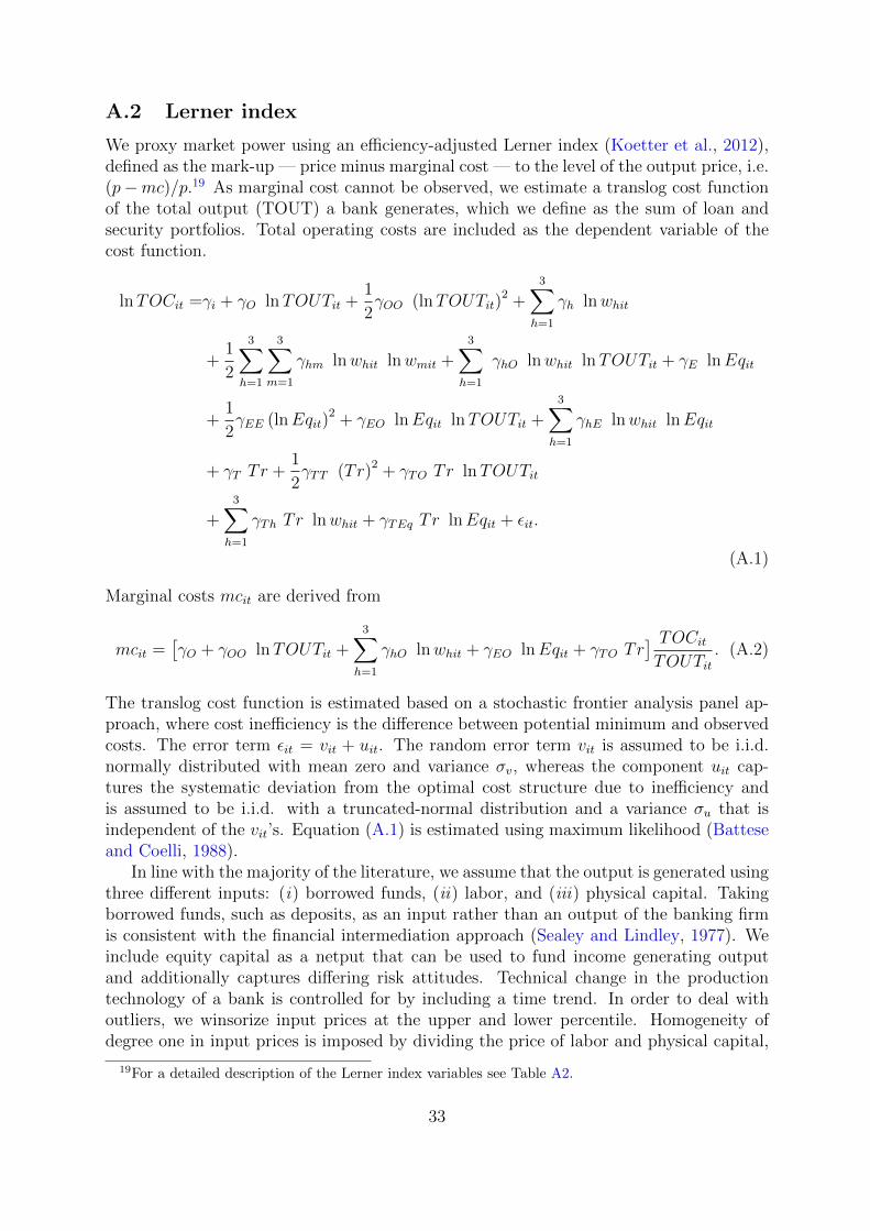
A.2 Lerner index

We proxy market power using an efficiency-adjusted Lerner index (Koetter et al., 2012),defined as the mark-up — price minus marginal cost — to the level of the output price, i.e.(p−mc)/p.19 As marginal cost cannot be observed, we estimate a translog cost functionof the total output (TOUT) a bank generates, which we define as the sum of loan andsecurity portfolios. Total operating costs are included as the dependent variable of thecost function.

lnTOCit =γi + γO lnTOUTit +1

2γOO (lnTOUTit)

2 +3∑

h=1

γh lnwhit

+1

2

3∑h=1

3∑m=1

γhm lnwhit lnwmit +3∑

h=1

γhO lnwhit lnTOUTit + γE lnEqit

+1

2γEE (lnEqit)

2 + γEO lnEqit lnTOUTit +3∑

h=1

γhE lnwhit lnEqit

+ γT Tr +1

2γTT (Tr)2 + γTO Tr lnTOUTit

+3∑

h=1

γTh Tr lnwhit + γTEq Tr lnEqit + εit.

(A.1)

Marginal costs mcit are derived from

mcit =[γO + γOO lnTOUTit +

3∑h=1

γhO lnwhit + γEO lnEqit + γTO Tr] TOCit

TOUTit. (A.2)

The translog cost function is estimated based on a stochastic frontier analysis panel ap-proach, where cost inefficiency is the difference between potential minimum and observedcosts. The error term εit = vit + uit. The random error term vit is assumed to be i.i.d.normally distributed with mean zero and variance σv, whereas the component uit cap-tures the systematic deviation from the optimal cost structure due to inefficiency andis assumed to be i.i.d. with a truncated-normal distribution and a variance σu that isindependent of the vit’s. Equation (A.1) is estimated using maximum likelihood (Batteseand Coelli, 1988).

In line with the majority of the literature, we assume that the output is generated usingthree different inputs: (i) borrowed funds, (ii) labor, and (iii) physical capital. Takingborrowed funds, such as deposits, as an input rather than an output of the banking firmis consistent with the financial intermediation approach (Sealey and Lindley, 1977). Weinclude equity capital as a netput that can be used to fund income generating outputand additionally captures differing risk attitudes. Technical change in the productiontechnology of a bank is controlled for by including a time trend. In order to deal withoutliers, we winsorize input prices at the upper and lower percentile. Homogeneity ofdegree one in input prices is imposed by dividing the price of labor and physical capital,

19For a detailed description of the Lerner index variables see Table A2.

33

as well as total operating cost by the price of borrowed funds. Output prices are assumedto be exogenously determined and given by total revenues to total assets.

The Lerner index can alternatively be written as (AR−MC)/AR, where AR representsaverage revenues and equals average profit plus average costs. In order to also integrateprofit inefficiencies into the Lerner index, we substitute total operating costs by profitsbefore tax (PBT) in Equation (A.1). Using predicted total operating costs and profitsbefore tax from these estimations, the Lerner index is calculated as (PBT +TOC−mc×TOUT )/(PBT + TOC).

The following table explains the variables included in the estimation:

Table A2: Variable description for Lerner index

Symbol Variable name DescriptionTOC Total operating cost Sum of interest, fee and administrative expensesPBT Profits before tax Profit before taxTOUT Total output Total earning output measured as the sum of interest-bearing assets

and securitiesw1 Cost of fixed assets Other administrative expenses excluding personnel expensesw2 Cost of labor Personnel expenditures to number of full time employee equivalentsw3 Cost of borrowed funds Interest expenses to total interest-paying liabilitiesEq Total equity capital Total regulatory capitalTr Time trend Time trend starting with 0 in the year 1999p Output price Total operating revenue to total assets

34

The Winner’s Curse - European Banking Authority Pausch...The Winner’s Curse Evidence on the...

Documents

Transcript of The Winner’s Curse - European Banking Authority Pausch...The Winner’s Curse Evidence on the...