Wind Resistance Generated by Containers on Reefer Vessels/Menu/... · Wind Resistance Generated by...
79
KTH Center for Naval Architecture
Transcript of Wind Resistance Generated by Containers on Reefer Vessels/Menu/... · Wind Resistance Generated by...

Wind Resistance Generated byContainers on Reefer Vessels
Master Thesis
CHRISTIAN [email protected]
KTH Center forNaval Architecture
STOCKHOLM
April 8, 2008

Abstract
The use of containers is steadily increasing and traditional container shipshave been taking market shares from the specialized reefer ships. The reefershipping industry loads its cargo on pallets that are loaded inside environ-mentally controlled cargo holds and reefer containers on the ships weatherdeck. The main concern of this investigation is to investigate the e�ectson the wind resistance generated from the varying deck load of containers.Speci�c ships in the NYKCool �eet are used to exemplify and quantify theresistances. This is done by modeling the wind resistance of a ship withvarying container loads using coe�cient estimations from Fujiwara et al.[2006] semi-empirical model. A wind load model is developed that gives fora full load of containers a mean increase of the total resistance of 1% whenaveraging over all wind directions. When also taking into account the lateralaerodynamic forces of the ship a mean increase of 4% is noted. Further aprocess to evaluate stored voyage data from ships performance and weatherconditions is developed and presented. The method is exempli�ed using thetypical reefer ships. Due to uncertainties in the database extract no conclu-sive results to support the wind load model could be found from the databaseanalysis.

Acknowledgments
The author would like to thank the following people for their contributionto this master thesis:
Brita Melén Eriksson, supervisor at NYKCool AB, for her guidance, adviceand help in retrieving material and deciding the path to take while workingon my thesis and this report.
Dr. Anders Rosén, examiner from the Center for Naval Architecture atthe Royal Institute of Technology, KTH, for his advice, teaching and con-structive comments during my �nal years at KTH and while working on mythesis and this report.
The sta� at NYKCool AB main o�ce for their assistance with my thesiswork, good company and for giving me the opportunity to work in the o�ce.
My family and friends for always encouraging me to do my best and giv-ing me assistance when needed.
Navigare necesse ist, vivere non necesse est!
-Pompejus
Solna, March 2008,
Christian Lindeen
2

Contents
1 Investigation 9
1.1 Background . . . . . . . . . . . . . . . . . . . . . . . . . . . . 9
1.2 Objectives . . . . . . . . . . . . . . . . . . . . . . . . . . . . . 10
1.3 Method . . . . . . . . . . . . . . . . . . . . . . . . . . . . . . 10
1.4 Wind load models . . . . . . . . . . . . . . . . . . . . . . . . 11
1.5 Comparisons of wind forces and hydrodynamic forces . . . . . 12
1.6 Database . . . . . . . . . . . . . . . . . . . . . . . . . . . . . 12
1.7 Studied ships . . . . . . . . . . . . . . . . . . . . . . . . . . . 12
2 Models 15
2.1 Wind load modeling . . . . . . . . . . . . . . . . . . . . . . . 15
2.2 Hull hydrodynamic resistance . . . . . . . . . . . . . . . . . . 23
2.3 Propeller forces . . . . . . . . . . . . . . . . . . . . . . . . . . 25
2.4 Force comparison . . . . . . . . . . . . . . . . . . . . . . . . . 26
2.5 Alternative factors . . . . . . . . . . . . . . . . . . . . . . . . 30
3 Database 31
3.1 Reported data . . . . . . . . . . . . . . . . . . . . . . . . . . . 31
3.2 Breakdown of analysis . . . . . . . . . . . . . . . . . . . . . . 34
3.3 Reliability of results . . . . . . . . . . . . . . . . . . . . . . . 44
3.4 Alternative analysis in database . . . . . . . . . . . . . . . . . 44
4 Comparison Model and Database 45
5 Conclusion 48
5.1 E�ect from containers on deck . . . . . . . . . . . . . . . . . . 48
5.2 The next step . . . . . . . . . . . . . . . . . . . . . . . . . . . 49
Bibliography 50
Appendix 52
A Fujiwara et al. [2006] wind force coe�cient calculations 52
3

B Holtrop-Mennen 57B.1 Resistance factor calculations . . . . . . . . . . . . . . . . . . 57
C Propeller force calculations 60C.1 Propeller non-dimensional coe�cients . . . . . . . . . . . . . . 60C.2 Taylor wake fraction, w . . . . . . . . . . . . . . . . . . . . . 60C.3 Force calculation . . . . . . . . . . . . . . . . . . . . . . . . . 61
D Data plots for selected states in database analysis 62D.1 Crown, Number of data points . . . . . . . . . . . . . . . . . 63D.2 Crown, I95% . . . . . . . . . . . . . . . . . . . . . . . . . . . . 66D.3 Family, Number of data points . . . . . . . . . . . . . . . . . 69D.4 Family, I95% . . . . . . . . . . . . . . . . . . . . . . . . . . . . 73D.5 Spread of I95% . . . . . . . . . . . . . . . . . . . . . . . . . . 77
4

Nomenclature
AF Frontal projected area [m2]
AL Lateral projected area of the hull [m2]
AT Area of immersed transom [m2]
ABT Cross-sectional area of the bulb [m2]
AOD Over deck projected area [m2]
B Breadth molded [m]
C Horizontal distance from G of the aerodynamic pressure center [m]
CB Block coe�cient []
CH Roll angle coe�cient[]
CM Midship area coe�cient []
CP Prismatic coe�cient of the ship []
CAK Roll wind moment coe�cient []
CAN Yaw wind moment coe�cient []
CAX Longitudinal wind force coe�cient []
CAY Lateral wind force coe�cient []
CWP Waterplane area coe�cient []
D Propeller diameter [m]
FP Propeller thrust force [N]
Fx Longitudinal force [N]
Fy Lateral force [N]
FALF Additional longitudinal drag []
5

FCF Cross-�ow drag []
FLF Longitudinal-�ow drag []
FXH0 Calm water resistance in x direction [N]
FXH Hydrodynamic hull force in x direction [N]
FXLI Lift induced drag x direction []
FY H Hydrodynamic hull force in y direction [N]
FY LI Lift induced drag y direction []
HFC Hourly fuel consumption [Tonnes/hour]
HC Vertical distance from waterline to the aerodynamic pressure center[m]
HL Mean lateral height [m]
HBR Bridge height from keel line [m]
I95% 95% con�dence interval [ton/h]
J Propeller advance ratio []
K Roll moment [Nm]
KH Hydrodynamic rolling moment around x axis [Nm]
KQ Propeller moment coe�cient []
KPT Propeller thrust coe�cient []
Loa Length overall [m]
Lpp Length between perpendiculars [m]
N Yaw moment [Nm]
NH Hydrodynamic yawing moment around z axis [Nm]
Q Propeller moment [Nm]
RA Model-ship correlation resistance [N]
RB Additional pressure resistance of bulbous bow near the water surface[N]
RF Frictional resistance [N]
RW Wave resistance [N]
6

RAPP Appendage resistance [N]
RTR additional pressure resistance due to transom immersion [N]
Rhydro Hydrodynamic resistance [N]
Sapp Surface area of rudder [m2]
T Draft summer load line [m]
UA Apparent wind speed [m/s]
UI Incident water speed at the propeller [m/s]
UT True wind speed [m/s]
Ukt Service speed [knots]
∆ Mass displacement [Tonnes]
ΨA Apparent wind angle [◦]
ΨT True wind angle [◦]
β Yaw angle of the ship [◦]
G Amidships section []
η0 Propeller e�ciency []
GM Transverse metacentric height [m]
φ Roll angle [◦]
ρA Air density [kg/m3]
ρh Water density [kg/m3]
σ Standard deviation [ton/h]
hb Height of the bulb from keel line [m]
k1 Hull form factor []
lcb Longitudinal center of buoyancy forward of G [m]
limconfint Con�dence interval limit []
n Number of data points []
n Rotational speed of propeller [rev/s]
qA Aerodynamic pressure [N ]
7

ux Longitudinal wind speed [m/s]
uy Lateral wind speed [m/s]
w Taylor wake fraction []
xi Residual fuel consumption [ton/h]
IFO Intermediate Fuel Oil [tonnes]
MDO Marine Diesel Oil [tonnes]
ME Main Engine
8

Chapter 1
Investigation
1.1 Background
The use of reefer containers is steadily increasing and traditional containerships have been taking market shares from the specialized reefer ships. Thereefer shipping industry loads its cargo on pallets that are loaded insideenvironmentally controlled cargo holds. Pallets can also be loaded into reefercontainers which are loaded on the weather deck of the reefer ships or onboardcontainer ships. To match the increased competition from container lines thespecialized reefer ships have increased their capacity for reefer containers.The competition also calls for e�orts in optimization of fuel usage and voyagerouting.
NYKCool apply a model for fuel consumption evaluation. This modeltakes into account both the hydrodynamic and aerodynamic resistance ofthe ship. Fuel consumption is modeled by taking into account the seagoingcharacteristics for typical reefer ships and correction factors for loading con-dition and for weather direction and force. The loading correction factor isexclusively dependant of the deadweight and not the volume of containers.
The weather correction factor relating to the weather force and directioncan be used to normalize the fuel consumption so it can be compared tostandard voyage conditions without the in�uence of weather. The correctionfactor does not take into account the variation of the wind resistance dueto the varying number of loaded containers on deck. To study the windresistance it is necessary to quantify how the wind a�ects a ship and use theseresults to expand or adjust the current models weather correction factor.
In the studies of wind induced forces and moments scaled tank test andsemi-empirical models are used. Several models are presented in the litera-ture and publications with varying degrees of complexity. Here the modelsby Fujiwara et al. [2006], Fujiwara et al. [2001], Blendermann [1994] and Ish-erwood [1972] are studied. The more modern models use regression analysisof scaled tank tests to produce equations that can be used to calculate the
9

wind related forces and moments for di�erent types of ships. In standardscaled resistance tank test a simple wind correction factor relating to thefrontal projected area of a ship is used to correct for di�erent wind speeds.This resistance usually only pertains to the ahead resistance which changesonly slightly when containers are added due to the frontal projected areaof the superstructure and ship. The lateral or side projected area, which isusually not included, is highly a�ected by the number of containers on deckproducing a substantial lateral force. The lateral force will produce a leewayas well as roll and yaw moments. The moments have to be balanced by theships hydrodynamics resulting in a change in the roll and yaw angles of theship.
1.2 Objectives
The main concern of this investigation is to investigate and quantify the ef-fects on the wind resistance from the varying deck load of containers. Windresistances for di�erent container loading conditions are calculated and inves-tigated. Of further interest is to compare these resistances with the hydro-dynamic resistance. A semi-empirical model is used to provide estimationsof the wind forces and their e�ects on a ship with containers. A comparisonof the modeled results with actual voyage data for several ships is made. Thevoyage data is analyzed with the aim of �nding trends in fuel consumptiondue to the loading of containers. The voyage data analysis results are inves-tigated as a possible veri�cation of the results from the calculation models.
Questions to be answered are:
• Does the number of containers greatly a�ect the resistance of the ship?
• Can trends be seen in the ships resistance for certain wind forces ordirections as well as ships draft or speed?
• Can actual voyage data be used to verify the theoretical results?
1.3 Method
To provide for a sound investigation several methods are required. A windload model is used to quantify the forces and moments acting on a ship.A variation of container loading conditions is used to �nd trends in theaerodynamic loading of a ship. Results are compared with hydrodynamicmodeling of the ships resistance. The model is implemented on varying reeferships in the NYKCool �eet. An analysis of voyage data for several ships isalso investigated to �nd trends in actual conditions on the fuel consumptionof the vessels. A comparison from voyage data with modeled total shipsresistance provides further insight into the e�ect of a varying deck load of
10
containers on the aerodynamic loading of the ships. General parametersused in the comparisons and modeling are the ships draft and speed as wellas wind force and direction while the number of containers loaded on theweather deck is varied.
1.4 Wind load models
Studies of the literature provide several models to estimate the wind resis-tance of ships. Most of these are semi-empirical and relate to wind tunneltests made on several di�erent types of ships. Fujiwara et al. [2006] presenta model based on the physical components of ship responses. Included arethe contributions from hull, rudder, propeller and above waterline structurein conjunction with the wind and sea state. Part of the model is the calcu-lations of wind induced forces and moments on a vessel. The model is basedon wind tunnel and towing tank tests. Actual ships parameters are used tocalculate the forces and moments. This wind load model is an extension ofthe model presented in Fujiwara et al. [2001].
Other models are also presented in literature. Isherwood [1972] presentsa semi-empirical model that provides for wind forces and moments basedon actual ships parameters but is based on a smaller sample of test datacompared to Fujiwara et al. [2006]. A later model is the one by Blendermann[1994] that is based on general coe�cients for several di�erent types of ships.Data for reefer ships or similar ships is not provided for. Both of these modelsdo not provide for di�erent parameters based on the projected area of theships hull and the projected area of the over deck structures and cargo.
The wind load model presented by Fujiwara et al. [2006] is here chosento model the wind forces and moments on the ship from the varying load ofcontainers due to several factors. Primarily it is claimed by Fujiwara et al.[2006] to have a higher accuracy level than the previously presented models.The number of basic ships factors needed is lower and the calculations morerational compared to Fujiwara et al. [2001]. Also the possibility to connectthe wind loads with the other physical components a�ecting the ship is ofinterest. The model can also be implemented directly to actual ships dimen-sions and parameters to calculate wind load coe�cients rather than usinggeneral coe�cients for di�erent types of ships.
The model is implemented in Matlab by The MathWorks Inc. [2007] sothat variables can be easily changed and adapted. In this way the codecan be used for several di�erent ships. Data sets can also be produced soas to facilitate comparisons with the database of previous journeys. Theimplementation of the model includes the ability to change the number ofcontainers loaded and their positions onboard.
11
1.5 Comparisons of wind forces and hydrodynamic
forces
In order to quantify the e�ects of containers onboard the ships a comparisonbetween the modeled wind loads and the hydrodynamic resistance of thehull is required. This is accomplished using the Holtrop-Mennen model ofships resistance. Using general ships data the hydrodynamic resistance iscalculated for the chosen example vessels. The results can then be usedto compare the hydrodynamic resistance and the aerodynamic resistancevariation caused by the varying number of containers.
1.6 Database
The main goal of the database analysis is to see if the data can be usedto study the e�ects from deck loaded containers on the fuel consumptionof the ships. This is quanti�ed in a plot of the hourly fuel consumptionagainst the number of containers on the weather deck. A further goal is todevelop a method to analyze the data and �nd trends in the e�ects fromdi�erent parameters. The outlining of trends is achieved by using states ofsimilar parameter conditions as a more quantative approach is possible whenrelating to data sets grouped into states instead of individual data points.Filtering is achieved as averages can be calculated for each state while stillkeeping a spread over the total data. The analysis method is also aimed atusing the trend results in a comparison with the theoretical wind load model.
The data compromise several vessels in the NYKCool �eet. The primarygoal is to �nd trends for the individual ships and not to do a general analysisfor the whole �eet. Many ships are sister ships and therefore it is advanta-geous to group these ships together and see if any trends arise for the classof ships.
The data is divided according to several factors. The division limits forthe factors are set up into groups in order to achieve a proper spread betweenthe states. These divisions are changed to include states that are relevantto the investigation or exclude less relevant states. Discretisation of data issuch that a proper number of data points are present in each state to achievea sound data spread.
1.7 Studied ships
Several ships are analyzed. The ships are chosen since they represent modernreefer ships with capability to load reefer containers on the weather deck andcan be seen in �gure 1.1. A table of ships particulars for the investigatedships can be seen in table 1.1.
12

(a) Crown
(b) Family
(c) Summer
Figure 1.1: Ships studied in the report. Photos courtesy of NYKCool AB.
13

Table 1.1: Ships data used in the modeling calculations.Ship class Crown Family Summer
Length overall Loa [m] 152 164 169
Breadth molded B [m] 23 24 24
Height of bridgefrom keel line
HBR [m] 19 22 21.6
Draft summer loadline
T [m] 8.7 10 9.5
Length betweenperpendiculars
Lpp [m] 139.4 150.6
Service speed Ukt [knots] 21 21 20
Container capacityon weather deck,empty containers
[FEU] 98 138 82
14

Chapter 2
Models
The Fujiwara et al. [2006] semi-empirical model takes into account the forcesfrom the hull hydrodynamics in both calm seas as well as in waves andcoordinates it with the wind e�ects into a steady state solution. The externalloads modeled are the longitudinal and lateral force, roll and yaw momentsusing the contributions from the hull, propeller, waves and wind. From themodel presented by Fujiwara et al. [2006] only the wind induced loads arecalculated. Hull hydrodynamic resistance forces are calculated using theHoltrop-Mennen method. Parameters for ship and on deck sources for windresistance are derived from general arrangements and loading plans. Theseare then used to calculate wind load coe�cients according to Fujiwara et al.[2006]. The coe�cients are used to calculate the wind forces and momentsacting on the ship. Wave induced forces are not calculated as only conditionsbetween 0-5 beaufort are part of the analysis. Propeller data and generalmethods for propeller force calculations are used to calculate the propellerinduced forces. The number of loaded containers and conditions a�ectingthe ships are varied to see how they a�ect the forces and moments acting onthe ships.
2.1 Wind load modeling
2.1.1 Model
The steady state equations that govern the motion of the ship around thecenter of gravity in longitudinal, lateral, yaw and roll degrees of freedom are:
FX = 0 (2.1)
FY = 0 (2.2)
N = 0 (2.3)
K −∆ ·GM sinφ = 0 (2.4)
15

here the de�nitions of the external loads acting on a ship are the longitudinal,FX , and lateral, FY , forces as well as the yaw, N , and roll, K, moments.These are oriented as seen in �gure 2.1. The mass displacement, ∆ andtransverse metacentric height, GM , together with the roll angle, φ, balancethe roll moment equation.
Figure 2.1: Coordinate system and de�nitions of force and moment signconventions for ship under wind loading, Fujiwara et al. [2006].
The components of the external forces and moments acting on a shipare identi�ed by Fujiwara et al. [2006] using subscripts as being the hull, H,propeller, P, rudder, R, wind, A, and waves, W. This results in the followingequations:
FX = FXH0 + FXH + FP + FXR + FXA + FXW
FY = FY H + FY R + FY A + FYW (2.5)
N = NH +NR +NA +NW
K = KH +KR +KA
The hydrodynamic loads on the hull are compromised of the calm waterresistance in x direction, FXH0, and the hydrodynamic hull loads FXH , FY H ,NH and KH . Hydrodynamic hull forces arrise when the ships are given ayaw, β, and/or roll, φ, angle. These are usually derived from towing tanktests. Since no towing tank test are available only the wind related forces andmoments are studied together with FXH0 and FP . FXHO is approximatedusing the Holtrop-Mennen method and FP according to general methods asdescribed in the following section. The wave and rudder induced forces arenot studied for reasons explained later in this report.
16

For the wind related forces and moments Fujiwara et al. [2006] calculatesestimations for the longitudinal-force coe�cient, CAX , lateral-force coe�-cient, CAY , yaw-moment coe�cient, CAN , and roll-moment coe�cient, CAK ,as follows:
FXA = CAX(ΨA)qAAF (2.6)
FY A = CHCAY (ΨA)qAAL (2.7)
NA = CHCAN (ΨA)qAALLOA (2.8)
KA = CHCAK(ΨA)qAALHL (2.9)
qA =12ρAU
2A (2.10)
HL =ALLoa
(2.11)
The coe�cients are dependant on the parameters presented in �gure 2.2 andin table 2.1. They are calculated using estimations by Fujiwara et al. [2006]presented in appendix A. The changes in position of the aerodynamic pres-sure and size of the projected areas when the number of containers is variedcan be seen in �gure 2.3. Variables describing the aerodynamic propertiesof the hull and superstructure are derived from General Arrangement plansas well as Capacity and Deadweight plans for each ship.
Table 2.1: Parameters used by Fujiwara et al. [2006] to calculate the windforce and moment coe�cients.
UA Apparent wind velocityρA Air densityAF Frontal projected areaAL Lateral (side) projected area of the hull
AOD Over deck projected areaqA Aerodynamic pressureHL Mean lateral height
HBR Bridge height from keel lineC Horizontal distance from G to the aerodynamic pressure center
HC Vertical distance from waterline to the aerodynamic pressure centerΨA Apparent wind angleCH Roll angle coe�cient
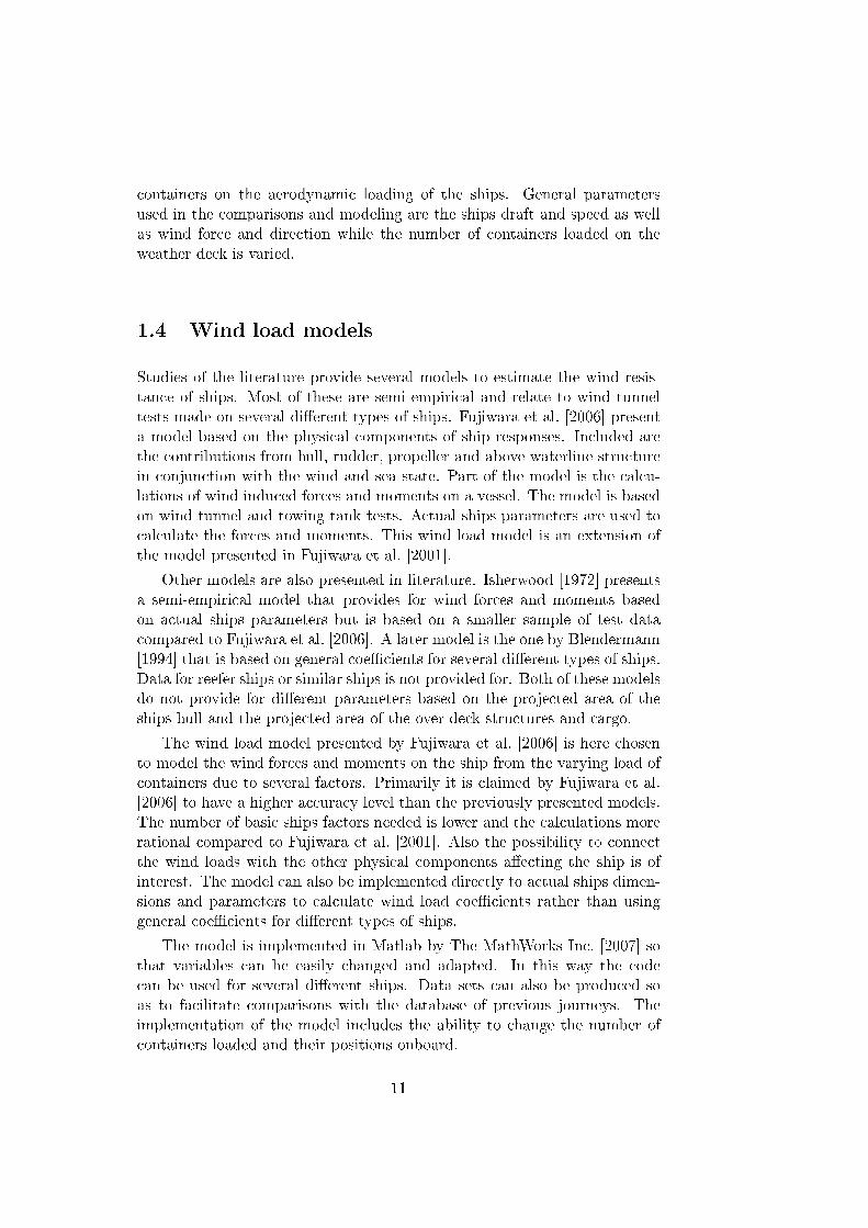
As seen in �gure 2.3 the addition of containers on the weather deck ofthe Crown and Summer ships has only minimal e�ect on the position ofthe center of aerodynamic pressure and the projected areas. For the Familyclass a large di�erence is noted as the center of dynamic pressure is furtheraft and moves steadily forward with the addition of containers. For all theship classes AF is not a�ected since the addition of containers generally fallswithin the bounds of the ships superstructure. A large increase in the lateral
17

Figure 2.2: Parameters used by Fujiwara et al. [2006] to estimate wind forcecoe�cients, Fujiwara et al. [2006].
above deck projected area, AOD, is seen upon the addition of containers. TheCrown class ships almost triple their AOD with 98 FEU1 loaded compared to0 FEU. The general increase in the total lateral projected area, AOD + AL,upon the addition of containers is generally between 36% to 47%. The shipshull lateral projected area AL is the largest area for all the ships but thesuperstructure and container area, AOD, can be of the same size upon theaddition of the full load of containers. The only major di�erence between theclasses is the position of qA for the Family class ships being further behindthan for the other ships.
2.1.2 Wind Pro�le
Relative wind velocity, UA, and direction, ΨA, are calculated using the lon-gitudinal, ux and lateral, uy wind speeds and the true wind speed, UT , shipspeed, US , and true wind angle, ΨT . Also the conventions of �gure 2.1 areused as follows:
ux = UT cos ΨT + US cosβuy = UT sin ΨT − US sinβ (2.12)
U2A = u2
x + u2y = U2
T + U2S + 2UTUS cos(Ψ + β) (2.13)
ΨA = tan−1 uxuy
= tan−1 UT cos ΨT + US cosβUT sin ΨT − US sinβ
(2.14)
How the wind pro�le of the apparent wind angle, ΨA, varies with truewind angle, ΨT , can be seen in �gure 2.4.
The apparent wind a�ecting the ships is highly in�uenced by the shipspeed. Two wind pro�le types can occur. The �rst case is when the windalways appears to come forward of amidships even when the true wind comes
1FEU: Forty foot Equivalent Unit, Standard measurement used to quantify the numberof 40 foot containers carried onboard.
18
(a) Summer, T=8 m, AL = 1088 m2, 40% increase in total lateral projected area, AL +AOD, due to containers.
(b) Crown, T=8 m, AL = 982 m2, 47% increase in total lateral projected area, AL +AOD,due to containers.
(c) Family, T=8 m, AL = 1202 m2, 36% increase in total lateral projected area, AL+AOD,due to containers.
Figure 2.3: Longitudinal distance of the aerodynamic pressure from G andsize of projected areas with varying number of forty foot container, FEU.
19
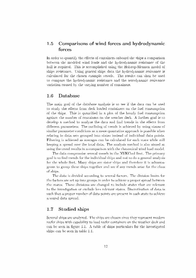
Figure 2.4: Wind pro�le for ships speed 20 knots and wind force 5 beaufort,averaged to 10 m/s.
from behind. The true wind speed is then not high enough in relation to theship speed to allow the apparent wind to come from behind the ship, insteadthe apparent wind speed is then greatly reduced. The second wind pro�lethat can occur is when the true wind speed is higher than the ship speedand the wind force assist the ship propulsion for true wind angles behindamidships. If the apparent wind came in from behind it then pushes theship forward and thereby producing a �negative� wind resistance.
For all the states studied in this investigation with UT below force 6beaufort and with US generally above 18 knots the wind pro�le always is suchthat the wind forces acts as added resistance and not as a propulsor. This isseen in �gure 2.4. The e�ect is that UA becomes minimal for astern windsand the wind loads become almost nonexistent for these directions. Theresulting e�ect of adding containers on deck in these conditions is thereforeminimal in comparison to when the UA is ahead or abeam.
These conditions change when the wind speed is increased above force 6beaufort or the ships speed is slowed below 18 knots. These new conditions,which are not studied, produce the e�ect that the additions of containershelp to reduce the ships resistance.
2.1.3 Assumptions
Several assumptions and parameters are here �xed in the calculation of thewind loads. The calculations are made for the three vessels to achieve aspread in results. The number of containers is varied from 0 to full loadof empty containers. The resulting change in the center of aerodynamicpressure and the longitudinal projected area is calculated. These are thenused to calculate a varying wind force and moment for di�erent numbers ofcontainers and wind directions. In order to make comparisons to the voyage
20
database the lateral and frontal area of the hull are compensated from thesummer draft conditions according to the examined draft in each case.
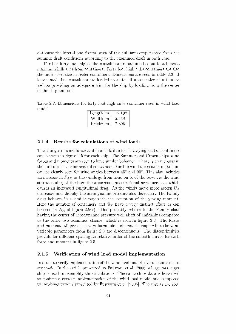
Further forty foot high cube containers are assumed so as to achieve amaximum in�uence from containers. Forty foot high cube containers are alsothe most used size in reefer containers. Dimensions are seen in table 2.2. Itis assumed that containers are loaded so as to �ll up one tier at a time aswell as providing an adequate trim for the ship by loading from the centerof the ship and out.
Table 2.2: Dimensions for forty foot high cube container used in wind loadmodel
Length [m] 12.192Width [m] 2.438Height [m] 2.896
2.1.4 Results for calculations of wind loads
The changes in wind forces and moments due to the varying load of containerscan be seen in �gure 2.5 for each ship. The Summer and Crown ships windforces and moments are seen to have similar behavior. There is an increase inthe forces with the increase of containers. For the wind direction a maximumcan be clearly seen for wind angles between 45◦ and 90◦. This also includesan increase in FAX as the winds go from head on to of the bow. As the windstarts coming of the bow the apparent cross-sectional area increases whichcauses an increased longitudinal drag. As the winds move more astern UAdecreases and thereby the aerodynamic pressure also decreases. The Familyclass behaves in a similar way with the exception of the yawing moment.Here the number of containers and ΨT have a very distinct e�ect as canbe seen in NA of �gure 2.5(c). This probably relates to the Family classhaving the center of aerodynamic pressure well abaft of amidships comparedto the other two examined classes, which is seen in �gure 2.3. The forcesand moments all present a very harmonic and smooth shape while the windvariable parameters from �gure 2.3 are discontinuous. The discontinuitiesprovide for di�erent spacing an relative order of the smooth curves for eachforce and moment in �gure 2.5.
2.1.5 Veri�cation of wind load model implementation
In order to verify implementation of the wind load model several comparisonsare made. In the article presented by Fujiwara et al. [2006] a large passengership is used to exemplify the calculations. The same ships data is here usedto con�rm a correct implementation of the wind load model and comparedto implementations presented by Fujiwara et al. [2006]. The results are seen
21

(a) Summer, Ukt = 20 knots, UT = 10 m/s, T = 8 m
(b) Crown, Ukt = 20 knots, UT = 10 m/s, T = 8 m
(c) Family, Ukt = 20 knots, UT = 10 m/s, T = 8 m
Figure 2.5: Changes in wind forces and moments on the ships.
22

in �gure 2.6. The results of Fujiwara et al. [2006] are replicated with onlyminimal di�erences. The di�erences are assumed to be caused by slight dif-ferences in input values and uncertainty on values not stated by Fujiwaraet al. [2006] and that are here approximated. The wind moment calculatedfor the exempli�ed ships is compared to the roll angle required to achievean equal hydrostatic righting moment. The resulting values are highly de-pendant on the guessed GM . These do fall within reasonable ranges andtherefore the calculated moments are assumed to be reasonable and withinproper margins for the analysis done.
(a) Fujiwara et al. [2006] results for largepassenger ship.
(b) Implementation of same ships data for largepassenger using implemented wind load model.
Figure 2.6: Comparison of coe�cients from Fujiwara et al. [2006] and imple-mentation of wind load model.
2.2 Hull hydrodynamic resistance
The hydrodynamic resistance of the Crown class is calculated according tothe widely used Holtrop-Mennen method. This is done to allow quanta-tive comparisons between the hydrodynamic and aerodynamic forces. TheHoltrop-Mennen method is described in Holtrop and Mennen [1978], Holtropand Mennen [1982] and Holtrop [1984]. This method is chosen since it usesbasic ship data and other factors relating to resistance of the hull to providefor a good estimation of the hydrodynamic resistance. The Holtrop-Mennenapproximation of the ships resistance, Rhydro, is calculated to approximatethe hydrodynamic calm water resistance, FXHO, acting on the hull. Theresistance components are divided into:
Rhydro = RF (1 + k1) +RAPP +RW +RB +RTR +RA (2.15)
where:
23

RF = frictional resistance1 + k1 = form factor of the hullRAPP = appendage resistanceRW = wave resistanceRB = additional pressure resistance of bulbous bow near the water
surfaceRTR = additional pressure resistance due to transom immersionRA = model-ship correlation resistance.
Calculation of the resistance components can be seen in appendix B.These calculations are done for the Crown class ships. No appendage otherthan the rudder is accounted for. Since the ships usually are not loadedto the load lines no additional resistance from the immersed transom is in-cluded. The hull hydrodynamic resistance calculations are done using thedata provided in table 1.1 and table 2.3. Linear interpolation of the hullhydrodynamic resistance from the mean drafts T = 4.5, 6, 8 is used to cal-culate the resistance for a speci�ed draft. In �gure 2.7 resistance curves canbe seen for the Crown class at typical drafts and speeds.
Table 2.3: Data used for the Crown class in the Holtrop-Mennen resistancecalculations
Mean draft T [m] 4.5 6 8
Block coe�cient CB [-] 0.4929 0.5260 0.5657
Midship area coe�-cient
CM [-] 0.9108 0.9331 0.9498
Waterplane area coe�-cient
CWP [-] 0.6029 0.6478 0.7265
Prismatic coe�cient ofthe ship
CP [-] 0.5411 0.5637 0.5956
Longitudinal center ofbuoyancy forward of G
lcb [m] 0.83703 1.3616 2.08727
Cross-sectional area ofthe bulb approximated
ABT [m2] 3.14
Height of the bulbfrom keel line
hb [m] 2
Surface area of rudder Sapp [m2] 23.107Area of immersed tran-som
AT [m2] 0
24

Figure 2.7: Holtrop-Mennen hydrodynamic resistance of Crown class
2.3 Propeller forces
A comparison between the total ships resistance and propulsive power isdone using the propeller thrust force. The e�ective propeller thrust force,FP , is calculated using propeller thrust diagrams produced by Lindgren andBjärne [1967] and presented by Garme [2007] together with the methods andcoe�cients presented in appendix C. For the Crown class ships data accord-ing to table 2.4 and the propeller thrust coe�cient, KPT , from Lindgren andBjärne [1967] is used to calculate the propeller thrust force, FP , de�ned as:
FP = KPTρD4n2 (2.16)
Calculations are made for a draft of T = 8 m resulting in a wake factorapproximation according to equation C.5 of w = 0.23 with results seen intable 2.4. The value in table 2.4 for the propeller force shows a good correla-tion with the total resistance calculated in the model when Rhydro is addedto FA.
25

Table 2.4: Propeller force characteristics and results for Crown classPropeller diameter D [m] 6.2
Propeller revolutions RPM [rev/min] 105
Number of blades 5
Expanded Area Ratio 0.61
Ships speed Ukt [knots] 21
Incidence speed UI [knots] 16.17
Advance ratio Jw 0.7667
Thrust force coe�cient KPT 0.2
Propeller Thrust FP [kN] 905
2.4 Force comparison
2.4.1 Wind loads
Several forces and moments are calculated for the ships being analyzed.These are the wind induced forces in longitudinal, FXA, and lateral, FY A di-rections together with wind induced moments in roll, KA and yaw, NA. Alsothe hydrodynamic resistance, Rhydro and the counteracting propeller force,Fp are calculated. Of interest is to study how these forces and momentschange when the number of loaded containers changes. This is done withoutchanging the ships draft and speed or wind force and direction. The changeis made in the projected areas and the position of the center of dynamicpressure corresponding to the addition of the containers. This counteractsthe change in draft usually arising from changes in the number of loaded con-tainers. These values can be seen in �gure 2.3. For all the ships examinedthe frontal projected area does not change upon the addition of containerssince the superstructure and other parts of the ships already covered thesesurfaces. Changes in the ships center of gravity are not examined as it doesnot a�ect the wind related forces.
The subject of this investigation is how much the di�erent wind inducedforces and moments change when containers are added. Therefore a meanvalue for wind directions 0◦ 6 ΨT 6 180◦ for each number of containers iscalculated for FXA, FY A, NA and KA. The average force and moment isthen compared to the baseline of 0 containers and plotted to see how thenumber of containers relatively a�ects the wind loads. This can be seen in�gure 2.8.
The addition of a full load of containers has a 10% to 30% relative increasein FAX . The lateral force FAY has almost a 40 to 50% relative increase. Thehigh relative increase in the lateral forces is to be given high considerationwhen doing comparison to the other forces acting on the ships.
The yawing moment for the Crown and Summer class ships have a similarbehavior. Here the relative shape of C from �gure 2.3 has a clear e�ect
26

(a) Summer
(b) Crown
(c) Family
Figure 2.8: Average wind forces and moments spanning over wind directions0◦ 6 ΨT 6 180◦ compared to baseline of 0 containers.
27

on the mean relative yawing moment. The high change for the last addedcontainers is due to the position of these containers being high up on theforedeck of the ships. For the Family class the true wind angle and the largesuperstructure produce a yawing moment which dramatically changes whenthe number of containers onboard is increased. The large lever arm producedby the position of the aerodynamic pressure center, C, has in this case a bigin�uence on the yawing moment.
2.4.2 Wind loads compared to hydrodynamic resistance
The in�uence of the containers compared to the hydrodynamic resistanceneeds to be compared to provide a clear understanding of how the varyingnumber of containers a�ect the ships total resistance and thereby the fuelconsumption. Just comparing the longitudinal forces is not enough since aship is a�ected by lateral forces when the wind a�ects the ship from di�erentdirections. The lateral forces cause a lateral drift as well as the rolling andyawing moments. To counteract these, the ship is given an incident anglerelative to the direction of travel in the water producing a lifting hydrody-namic force. This results in an increased drag on the ship in the longitudinaldirection. To approximate the e�ects of this on the ships total resistance andthe e�ect from the increased lateral wind force due to a changing number ofcontainers a total wind force, FA, is calculated using:
FA =√F 2XA + F 2
Y A (2.17)
This approximation probably overestimates the e�ect from the lateral windforce since no compensation is made for the ship having a leeway or hydro-dynamic lifting force due to an incident angle of the hull to the water.
In �gure 2.9 FA and FXA are compared relative to Rhydro with meansover 0◦ 6 ΨT 6 180◦ for each added container. The maximum and minimumvalues are also presented. Rawson and Tupper [2001] state that the aerody-namic resistance can be 2-4% of the total resistance in full speed conditionsif no wind is present and quadrupled to 4-16% if there is a head wind of thesame speed as the ship. The �gure 2.9 shows that when only the longitu-dinal forces are studied the aerodynamic resistance is up to 15% of Rhydroas would be expected. If the lateral wind forces also are accounted for theaerodynamic resistance it up to 30% of Rhydro. It is therefore of interest tostudy how this relationship changes upon the addition of containers. Themean values and the maximum values show a very slight increase when thenumber of containers is increased.
To isolate the e�ect from containers the relative change in total resistance,Rtot, compared to the baseline of no containers is calculated for both Rtot =FAX +Rhydro and Rtot = FA+Rhydro. Results are shown in �gure 2.10. The�gure shows how the addition of a full load of containers changes the total
28

Figure 2.9: Comparison between the aerodynamic and hydrodynamic resis-tances for Crown class with US = 20 knots, UT = 10 m/s and T = 8 m. Inthe left �gures the max, mean and min is calculated over 0◦ 6 ΨT 6 180◦. Inthe right �gure the max, mean and min is calculated over all the containers.
Figure 2.10: Max, mean and min e�ect on the total resistance from contain-ers. In the left �gures the mean is calculated over all the wind angles. Inthe right �gure the mean is calculated over all the containers.
29

resistance. On average a 1% increase is noted when only looking at forces inthe x direction. When also taking into account FAY a mean 4% increase isnoted. These are the �gures that best represent the e�ect from a full loadof containers on the resistance of the Crown class.
In general it can be said that the addition of containers on deck causesan increase in the forces a�ecting the ship even when the wind comes fromastern. Since the apparent wind never comes from behind in the typical shipsspeed and wind range studied the addition of containers does not reduce thetotal resistance. The variation of the wind angle has a large e�ect on therelative size of the aerodynamic and hydrodynamic forces. The highest e�ectof the wind angle after being averaged over all container conditions is seenfor wind conditions between of the bow and abeam.
2.5 Alternative factors
Are there other factors that are not taken into consideration that could a�ectthe results? By doing the calculations for wind forces below 6 beaufort it isassumed that the e�ect from the waves is minimal. In the wind load modelfactors that are not accounted for are the rudder and wave induced forces.Introducing the rudder forces would also provide for the need to take intoaccount the lifting force from the hull. This lifting force arises when the hull isgiven an incident angle to the in�owing water. The lifting force balances theyawing moment and lateral force from the wind. The resulting induced dragon the hull would then be a complement to the calculation of forces a�ectingthe hull. An attempt to take this into account is done when comparing theaerodynamic force FA to Rhydro. Further when the ship is given a roll angledue to the wind load Rhydro will change. These are the hydrodynamic loadsFXH , FY H , NH and KH presented by Fujiwara et al. [2006] whom also statethat these forces can become substantial and a�ect the ships speed. Anotherfactor that can be discussed is the stacking order and position of containers.This might have an e�ect on the aerodynamic character of the ships whichchanges the relationships governing the approximations for the wind loadcoe�cients. Since it was assumed in the model that the containers wereloaded in a basic way, based on stability, this need not be a factor.
30

Chapter 3
Database
A parallel investigation to the theoretical process is made through analysis ofstored vessel voyage data. The method for database analysis is here outlinedand applied on a database extract. The aim is to make a qualitative analysisof e�ects on the IFO1 and MDO2 ME3 fuel consumption due to the addedwind resistance from containers on the weather deck.
3.1 Reported data
The data consists of several vessels daily reports from voyages over severalyears. Each day the ships masters report the status of the ship and theweather conditions. This is then stored by the land organization for evalua-tion and follow-up of the ships. Two classes of ships are analyzed from thedatabase. For the Family class four sister ships daily voyage data is usedfrom the latest eight years compromising 11785 data points. Five ships inthe Crown class with voyage data from the latest four years compromising7923 data points are used. The fuel consumption against the number of con-tainers for both ships can be seen in �gure 3.1 for all data points. A widespread can be seen for both classes. This is caused by the large variation inthe loading conditions and in uncertainties in the reported data as discussedin the following sections. For the Crown class a slight increasing trend can benoted. The variations for the Family class are larger and no trend is clearlyvisible which might pertain to the Family class having a variable pitch pro-peller, VPP. The VPP highly a�ects the fuel consumption of the ships as theengines can be run at a higher e�ciency for more loading conditions thanthe Crown class �xed propellers.
1IFO: Intermediate Fuel Oil are fuels blended from diesel and bunker fuels classi�edinto di�erent grades as speci�ed by the universally adopted SI (System International d'Unites) metric system of measurement. Petron [2007]
2MDO: Marine Diesel Oil3ME: Main Engine
31

(a) Crown
(b) Family
Figure 3.1: Fuel consumption against number of containers for Crown andFamily class ships. All data points.
32

The reported data consists of estimated and measured values collectedby the crew. Only the data used in conjunction with this report is discussed.Constant data for each voyage is the number of containers onboard. Thereports only contain the number of containers loaded on the weather deckand not their positions. Recorded data is seen in table 3.1.
Table 3.1: Recorded data from ships daily reportsData Units Comment
Date daySailed time h
Sailed distance NmSpeed knots
IFO consumption tonesMDO consumption tones
Wind force Beaufort 24 h meanWind direction See �gure 3.2 24 h mean
Propeller revolutions RPMDraft fore and aft m
Figure 3.2: Wind direction codes. Calm = 0, Variable = 9
Measurements are made by the crew on a daily basis. The main partsof the measurements are to be taken as having rather high accuracy. Mostof the measurements are made manually and this can have an e�ect on theresults. Care is to be taken into data sets where special conditions applythat brings the data outside of the objective of this investigation. Suchcircumstances are transits to and from harbors and sea passages, increasedresistance due to changes in hull and propeller conditions before and afterdocking. Other factors that a�ect the accuracy of the results is the lack of
33
container positions in the reports.
A discrepancy is noted in the extracted data that a�ects the conclusivenature of the results in this report. As can be seen in �gure 3.1(a) for theCrown class ships there are several data points where the reported numberof FEU containers on deck highly exceeds the maximum loading conditionof 98 FEU. For the Family class the number of data points exceeding themaximum number of 138 FEU only accounted for a few voyages. For theFamily class voyage data is compared to another NYKCool database andit is found that the majority of the examined container on deck �elds areerroneously reported into the voyage database. Possible causes for the wrong�gures in the voyage database can be tracked down to a mix of FEU andTEU4 containers being reported instead of the equivalent number of FEUs.Further some containers carried by the ship were loaded in the cargo holdsand these containers were reported in the voyage database as being on deck.
The comparison with the second NYKCool database is done for 29 voy-ages of the Family class. These voyages are spread over the whole span ofcontainer loading conditions with emphasis on the voyages over the shipsmaximum on deck FEU loading. Most of the data for FEU containers ondeck is found to be wrongly reported or can not be checked. The voyageswhere correct data is found are corrected but this is only a small amountof voyages compared to all data points. The corrected values are the onesplotted for the Family class in �gure 3.1(b). The Crown class data pointsare assumed to have the same bad reliability when it comes to the number ofreported containers on deck. Because of these di�erent sources of uncertain-ties in the database the focus in this report is on developing a methodologyfor �nding trends from database results rather than actually �nding trendsapplicable to the exempli�ed vessels.
3.2 Breakdown of analysis
In order to calculate the fuel consumption dependency on the numbers ofloaded containers the database data has to be prepared for analysis. A dia-gram of this algorithm is presented in �gure 3.3 with a detailed explanationin the following sections. Here a short description is made. Firstly the datais sorted into states, by state meaning a set spread of factors and conditionsa�ecting the ships fuel consumption. Each data point is sorted into a speci�cstate if the factors and conditions represented by the data point fall withinthe set spread of sorting factors for that state. An even spread of data intothe states is assured by choosing limits for the sorting factors a�ecting thefuel consumption. The spread in conditions for each state is represented bythe intervals in the sorting factors. Once the data is sorted into states a
4TEU: Twenty foot Equivalent Unit, Standard measurement used to quantify the num-ber of 20 foot containers carried onboard.
34
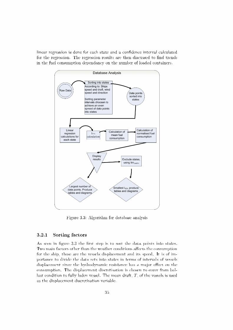
linear regression is done for each state and a con�dence interval calculatedfor the regression. The regression results are then discussed to �nd trendsin the fuel consumption dependancy on the number of loaded containers.
Figure 3.3: Algorithm for database analysis
3.2.1 Sorting factors
As seen in �gure 3.3 the �rst step is to sort the data points into states.Two main factors other than the weather conditions a�ects the consumptionfor the ship, these are the vessels displacement and its speed. It is of im-portance to divide the data sets into states in terms of intervals of vesselsdisplacement since the hydrodynamic resistance has a major e�ect on theconsumption. The displacement discretisation is chosen to cover from bal-last condition to fully laden vessel. The mean draft, T , of the vessels is usedas the displacement discretisation variable.
35

The next part of the sorting step is to divide the data according toships speeds. Ships are ordered to maintain a certain speed depending onthe nature of the time table and cargo type onboard. Further the shipscrew might choose to lower the speed due to weather conditions or otherfactors. The ships speeds are highly in�uenced by the hulls free streamingand wave making resistance. The usage of ships speed to sort the datapoints means that both the hulls free streaming and wave making resistanceis accounted for. The ships speed, US , is used as the discretisation variablefor hydrodynamic resistance.
The wind force has an e�ect on the fuel consumption and speed of thevessels. Since the wind force is reported in beaufort a �rst division is madeaccording to the beaufort scale. An upper limit for the wind force is used.This since the wave induced resistance will start to have an e�ect on theships performance as well as the crew opting to voluntarily reduce speedwhen the wind force is high. The upper limit is set to include data up tobeaufort force 5.
A division according to wind direction also has to be done. The symmetryof the vessels is used to sort data points into states according to table 3.2using direction codes presented in �gure 3.2.
Table 3.2: Wind direction grouping according to wind direction codes.Wind direction codes
Ahead wind 1,0,9Of the bow wind 2, 8
Beam wind 3, 7Of the stern wind 4, 6
Stern wind 5
Each state now represents a group of data points with similar conditions.The main remaining factor that di�erentiates the data within a state is thenumber of containers loaded on the weather deck and the fuel consumptionwhich is the basis for the following analysis. Other factors still remain such asthe swell size and direction, ships trim, and time since dry docking amongstothers. These are in this �rst basic analysis disregarded. The usage of windforce and direction, ships speed and draft will provide for a good basic �rstanalysis which is the aim of this investigation.
3.2.2 Interval selection
The four main sorting factors for placing data points into states are thus theships speed and draft, wind direction and wind force. Each state comprisesdata points sorted according to intervals of these four sorting factors. Thesizes of the intervals are di�erent but keeping an even number of data pointsin each interval is prioritized to keep balanced intervals. The intervals are
36

chosen in both length and number so that the data points are evenly spreadover the ships speed and draft. Wind direction and force are already in aninterval grouping and kept that way.
A spread of the data for the Crown and Family class ships can be seenin �gure 3.4. Two counteracting factors a�ect the choice of interval. The�rst is the need for a high number of data points in each state so thatthe linear regression has a high number of data points which provides for astable regression. This demands wide intervals to get a high number of datapoints in each state. The second counteracting factor is the need for distinctresults so that a continuous analysis over varying conditions can be appliedwith consistent and smooth results. This demands that the intervals be madeas small as possible and increased in number. The smaller the intervals thelarger the number of states thus leading to the data points being spreadthinly into all the states and thereby not allowing for accurate regressionsdue to lack of data points.
3.2.3 Linear regression
The second step in �gure 3.3 is to do a linear regression. Once the datapoints are sorted into states an analysis is made within each state to �nd thedependancy of the ME fuel consumption against the number of containersloaded on the weather deck. The mean Hourly Fuel Consumption, HFC, iscalculated for each data point. The usage of IFO is predominant throughoutthe voyage data. The HFC is then compared to the number of contain-ers on deck. From the theoretical studies a linear dependency is observedin the forces. Therefore for the database investigation a �rst degree poly-nomial is the assumed dependency of the number of containers on the fuelconsumption. Further the interval or span of the conditions within a stateare small. This means that a linear approximation of the dependency of thefuel consumption on the number of loaded containers is a viable if simpleapproximation.
For each state a linear regression is made using the method of leastsquares on a �rst degree polynomial. The inclination of this line representsthe HFC/container coe�cient with the unit tones of fuel per hour percontainer. This coe�cient represents the e�ect of containers on the fuelconsumption. The linear dependency is plotted onto the data points in eachstate to see the congruence of the data points and the regression, see �gure3.5. Further the residuals, xi, being the distance from the regression line andthe data points is calculated. The standard deviation, σ, of the residuals iscalculated and used in the calculation of a 95% con�dence interval, I95%.
37

(a) Crown
(b) Family
Figure 3.4: Spread of the data points for both Crown and Family class ships.
38

This is done using:
σ = (1n
n∑i=1
(xi − x)2)12 (3.1)
x =1n
n∑i=1
xi (3.2)
I95% = λα/2σ√n
(3.3)
where n is the number of data points within the state on which the regressionis based, λα/2 = 1.6449 for the assumed normal distribution and for a 95%con�dence interval and where x is the mean for the residual. By 95% con�-dence interval it is meant that 95% of the residuals fall within the con�denceinterval from the regression line. The con�dence interval is here calculatedand used to give a general assumption of the quality of the regression, notas a con�dence interval for the regression itself. The smaller the con�denceinterval, the better the regression curve is �tted to the data points in thestate and the higher the concentration of data points around the regressioncurve. The con�dence interval is not meant to be a quantative measure tobe used in the calculation of coe�cients but rather as a qualitave measureto how accurate the regression coe�cients are.
3.2.4 State selection for comparison
In order to �nd trends in the data a selection is made to study the stateswith the highest accuracy and quality as well as trends over several states toachieve a general conclusion. Two criteria are chosen to pick out the stateswith the highest accuracy and quality in the regression. Firstly the number ofdata points in the regression and secondly the size of the con�dence interval.The more points used in a regression the better the regression. A problemarises if the spread of the data points is high, due to erroneous data, resultingin a loss of quality in the regression.
Using the con�dence interval as a selection criteria means that the stateswith the lowest con�dence interval are the ones with the best quality of re-gression results. The con�dence interval will decrease in size with increasingnumber of data points in the state but also having very few data pointsresults in a small standard variation producing a small con�dence interval.These states of few data points have to be �ltered out in the analysis sincethe few data points do not produce indicative regressions for that state.Therefore when the con�dence interval is used as selection criteria a lowerlimit, limconfint, for the number of data points in a state is used in the se-lection process. The limconfint is presented in the �gures when used and isgenerally around 10 data points. The e�ects of this is seen in section D.5.
39

The two selection criteria are used to pick the 18 states with highest num-ber of data points and the 18 states with the smallest con�dence interval.This is done for grouped data for wind forces 0-5 beaufort and 0-2 beaufortfor the Family and Crown class. In �gure 3.5 examples for both the highestnumber of data points in a state and the regression with the smallest con�-dence interval, I95%, are presented for both ships. Complete �gures for the�rst 18 states selected according to the number of data points and smallestI95% is presented in appendix D. The results for the selected states is foundin tables D.1 to D.6. In appendix D.5 the spread of I95% is presented as wellas the choice of lower limit, limconfint, for the number of data points usedin the selection according to I95%.
(a) Family, Highest number of datapoints
(b) Family, Smallest I95%
(c) Crown, Highest number of data points (d) Crown, Smallest I95%
Figure 3.5: States with most data points for regression and the smallestcon�dence interval, I95%, for Crown and Family class. Wind force span forselection of data points 0-5 beaufort.
Another possible way of selecting states which can be used to draw con-clusions on the fuel dependency of containers on deck is to do a convergenceanalysis. This is achieved by studying the coe�cients in the regression anal-ysis using smaller sample sets for the regression calculations. Then withadded number of data points the coe�cients converge to certain values. The
40

rate of convergence and relative change in size of the coe�cients can be usedto ascertain when a coe�cient has achieved the required accuracy and qual-ity. It is also possible to select states on this basis of fast convergence todo further analysis. This convergence analysis is implemented but no resultsare presented since no good and consistent results are found due to lack ofdata points and accuracy.
3.2.5 Discussion
In the implementation on the Crown and Family class ships a conclusioncould not be made over all states. This since not enough data points couldpopulate all states and still have a linear regression with a good con�denceinterval for each state. A possible solution is to increase the interval foreach state but then the spread of the data points grows and the linear ap-proximation is no longer based on the container number to fuel consumptionrelation but also on the sorting factors themselves. The methods for selec-tion of states still provide for a good means of comparison since they takeinto account the number of data points used in the regression as well as thespread of these data points.
Further for the implementation it can be seen in the result tables ofappendix D that the �rst degree polynomial regression used within each statedoes not provide for a conclusive �gure on the FHC/container coe�cient.For both the Family and Crown class the e�ect of changing the numbers ofcontainers is inconclusive in this analysis having both negative and positivecoe�cients and no general trend can be seen. What can be seen is that themagnitude of adding or removing one container provides for a change in thefuel consumption by either increasing or decreasing the fuel consumption by0.01-1 kg of fuel per hour. This translates into a %��to % change in the totalfuel consumption for each container added. There is not even any trendwhen looking at the sorting factors on when the FHC/container coe�cientchanges sign.
If only the lower wind speeds of 0-2 beaufort are used in the analysis nonew results arrise. For the Crown class too few states are populated withenough data points to give any viable results. The Family class has morehighly populated states but does not provide any conclusive initial trends.
Several things could be a�ecting the fact that no trend is seen for the fuelconsumption coe�cients. The main factor is thought to be the uncertaintyin the reported values of containers on deck. Further factors could be thatthe intervals set for the speed and draft are too wide and that a smallersubdivision into states is necessary. Also a larger database extract might benecessary.
41

3.2.6 Trends over several states
To study trends over several states the FHC/container coe�cient is studiedfor �xed conditions for one of the sorting factors, while the others are varied.The aim here is to �nd trends for a variation in each sorting factor. This isaccomplished by identifying the states for a set value of one of the sortingfactors and calculating the mean coe�cient value, mean number of datapoints and mean con�dence interval for these states. This then includesvalues for a variation of all the other sorting factors and makes it possible toisolate the e�ect of a certain sorting factors. In this manner it is possible to�nd general trends for each of the sorting factors. The mean value of I95%
for the regression is also calculated in the same process and used as a way ofmeasuring the relative accuracy of the comparison. Figure 3.6 shows thesemeans for the Crown and Family class ships in the division into states usingwind forces 0-5 beaufort.
It is seen that most of the means are >0. This falls in line with the windload model results that the addition of containers should increase the fuelconsumption. The means that were <0 for the Crown class are when thedraft is shallow at 4.95 m and when the wind direction is astern. Also thehighest ship speed at 22 knots gave a mean decrease in the fuel consumptioncoe�cient. A possible explanation for these results is that at these pointswhen the aerodynamic pressure is large and the lateral cross-sectional areais large the addition of containers causes a slipstreaming e�ect for Crownclass ships when the wind has a more rounded body to move over. This thendecreases the fuel consumption.
The Family class showed general increase in fuel consumption for themeans for each sorting factor except for the largest draft at 8.675 m and lowwind forces of 0 and 2 beaufort. For the low wind speeds to give an e�ect oflowering the fuel consumption upon the addition of containers it might bedue to a more aerodynamic and slipstreamed form as the Family class havea large square superstructure. At the low wind speeds the apparent winddirection is for the most part straight ahead and the containers then providefor a more slipstreamed frontal projected area.
42

(a) Crown, WindD = Wind direction code, WindF = Wind force beaufort, Speed in knots anddraft T in m.
(b) Family, WindD = Wind direction code, WindF = Wind force beaufort, Speed in knots anddraft T in m.
Figure 3.6: E�ects of the isolated sorting factors on the fuel consumptioncoe�cient. Wind force division 0-5 beaufort.
43

3.3 Reliability of results
The use of the voyage database to verify the results of the wind load modelwould be ideal. However due to the uncertainty in the quality of the reportednumber of containers on deck the results done from the database analysis arenot conclusive. To just remove the data points that lie outside the maximumrange of allowed FEU on deck is not an option. The data points that wereindependently checked showed there could be a lot of wrongly reported pointswithin the selected data sets. Since the �gure of containers on deck is criticalto the work in this investigation a big uncertainty arises in the assumptionsmade from the database analysis.
3.4 Alternative analysis in database
If no trends can be found in the data alternate methods could be explored.One method is to make corrections in the data sets by normalizing for thesorting factors and other factors. It can be assumed that within the smallstates of data sets the fuel consumption due to displacement, speed andweather behaves linearly. By making a linear regression within the states forthe ships draft and speed, wind forces and directions a correction factor forthe consumption valid for the data points within that state can be calculated.The consumption is then normalized within the state and only the numberof containers loaded will be left as a factor. Another possible method is tomake a regression for the ships whole data. The curves can then be used tonormalize the consumption according to ships draft and speed, wind forcesand directions so as to leave the number of containers as sole factor.
Further factors can be analyzed and used to sort the data points usedin the analysis. Factors that might reduce the quality of the measurementsare the engine, hull and propeller conditions of the ships. Also since theships are docked and serviced periodically it might be necessary to removedata sets around the time of docking since hull condition will then have anadverse e�ect on the analysis.
44

Chapter 4
Comparison Model andDatabase
The use of the database results from the previous chapter to verify the resultsof the wind load model produced in chapter 2 is here discussed. The valuesbeing compared are factors of di�erent types. The model provides for afactor that describes how much the total resistance changes for a certain statewhen containers are added and relates to the forces involved. The databaseprovides for each state a factor of change in fuel consumption dependent ona change in number of containers. A comparison between these two factorswill not provide for a numeric veri�cation but an indication of the trends.
In order to compare the theoretical results to the database, wind loadmodel calculations are made for speci�c states. For these states the windforces FA and FAX are modeled and compared to the hydrodynamic resis-tances. The total resistance for both aerodynamic forces is calculated usingrespectively:
Rtot = Rhydro + FA (4.1)
Rtot = Rhydro + FAX (4.2)
The total resistance will change with the addition of containers due to thechange in the aerodynamic forces. To better isolate the e�ect of addingcontainers on the total resistance a baseline total resistance is calculatedusing the aerodynamic forces when no containers are loaded as follows:
RF0 = Rhydro + FA(0 containers) (4.3)
RF0 = Rhydro + FAX(0 containers) (4.4)
The aerodynamic forces from the containers is then isolated from theships aerodynamic forces and used to calculate a relative e�ect usingFcontainers/Rtot and Fcontainers/RF0. An average linear relative e�ect fromthe addition of containers and the inclination coe�cient, ∆FAcontainers/Rtot,is also calculated for each case. Figure 4.1 shows an example of these �gures.
45

Figure 4.1: Relative e�ect from containers on the aerodynamic force com-pared to the hydrodynamic force
From the database analysis the HFC/container coe�cient, from sec-tion 3.2.3, is normalized using the mean HFC within the state to calculatethe relative e�ect of the addition of containers on the fuel consumption.This factor is named ∆HFC/container. This is compared to the factor∆FAcontainers/Rtot calculated as above for the conditions in each state forthe Crown class and presented in table 4.1. A comparison between the tworight columns shows that no clear correlation can be seen for the coe�cientsfrom each state in the database extract and the corresponding modeled co-e�cient. The results from the database extract are clearly a�ected by theuncertainties and discrepancies mentioned in section 3.1.
The only conclusion that can be made is that a change produced by eachcontainer is a change by 0.001 to 0.01% in the forces and fuel consumption.If this is compared to the full load of containers less than 1% relative changeis produced in the states to be compared with the similar results in section2.4.2. The modeled forces all produce a relative increase while the fuelconsumption according to the analyzed database extract is very random toif it is a relative increase or decrease.
46

Table 4.1: Comparison of relative fuel consumption coe�cient∆HFC/container with wind model forces ∆FAcontainers/Rtot. Com-parison made for Crown class with selection based on I95% and wind forces0-5 beaufort.Wind Wind Mean Mean ∆HFC/container ∆FAcontainers/RtotDirection Force speed T Database Wind load model
1 3 20,5 7 3,70E-04 8,46E-061 4 19,5 7 1,68E-04 1,23E-051 4 19,5 7,95 5,76E-04 1,03E-051 4 20,5 7 2,23E-04 1,12E-051 5 19,5 7 3,06E-04 1,63E-051 5 19,5 7,95 5,12E-05 1,39E-052 3 20,5 7 -7,28E-06 2,49E-042 3 22,2 4,95 -8,48E-04 3,00E-042 4 19,5 7 3,40E-04 5,26E-042 4 19,5 7,95 -4,56E-05 4,54E-042 4 20,5 7 -5,99E-04 4,67E-042 5 19,5 7,95 -1,48E-04 7,46E-043 4 20,5 7 -7,89E-05 5,87E-044 3 20,5 6 1,61E-04 2,12E-044 3 20,5 7 1,67E-04 1,76E-044 4 20,5 6 -1,48E-04 3,21E-044 4 20,5 7 -8,52E-05 2,70E-044 5 20,5 6 1,68E-04 4,31E-04
47
Chapter 5
Conclusion
5.1 E�ect from containers on deck
In order to study the e�ects from loading containers on the weather deckof ships this investigation had two parts, a wind load model and a voyagedatabase analysis. For the wind load model the ships speeds were generally20 knots with a draft of 8 m and a wind speed of force 5 beaufort. The windload model gave reasonable results that the longitudinal aerodynamic forcesincrease by 10% with the addition of a full load of containers. The lateralaerodynamic forces have an even larger increase of up to 40%. However theseforces have to be put into relation with the hydrodynamic resistance of thehull. When looking at the e�ect of a full deck load of FEU containers onthe total resistance of the Crown class ships the wind force model providesfor an increase of 1% when averaging over all wind directions. When takinginto account the lateral aerodynamic forces a mean increase of 4% is noted.However since the lifting force of the hull is not taken into account to balancethe lateral aerodynamic force an assumption can be made that the e�ect ofa full load of containers on the ships total resistance is between 1 and 4%.This means that the relative e�ect of loading one container onboard is thatthe wind forces will increase by 0.01 to 0.04%.
The second part of the investigation was to do an analysis of voyagedata stored in a database. A method was presented in this report whichprovides for such an analysis. This was done by dividing the data in statesof similar data points were certain conditions are kept within intervals. Theseconditions are the ships draft and speed while also sorting the data accordingto the prevailing wind direction and force. For each state a linear regressionwas made of how the fuel consumption varies with the addition of containers.By then looking at the linear regressions for di�erent groups of states aconclusion of the fuel consumption under certain conditions could be made.This process was done to data for the Family and Crown class. Howeverdue to uncertainties in the database material it was not possible to draw
48

any conclusive results. Neither was it possible to con�rm the results fromthe wind model predictions. The results indicate that a change in bothincrease and decrease in fuel consumption due to containers is in the order ofmagnitude between 0.01-1 kg of fuel per hour for each loaded container. Thishas to be taken into relation that the mean fuel consumption is between 1.4-1.9 tones per hour for the ships. The relative change in the fuel consumptionis then in the same order of magnitude as the change in the forces modeled.
5.2 The next step
Several aspects can be addressed for continuation of this investigation. Forthe wind force model it is possible to expand the model with the rudderforces and the e�ects of an incident angle on the hull to the hydrodynamicforces. The e�ects of di�erent con�gurations of containers with respect toaerodynamic slipstreaming and the e�ects of turbulence could also be exam-ined. For the database analysis it would be interesting to improve the datacollection and thereby do a proper comparison to the wind load model. Thesub division into states can be further re�ned by normalizing the fuel con-sumption within in each state for the exact values of the sorting factors. Thiscould also be done for the whole data set by using non dimensional factorsand use this to compare ships from di�erent classes. Another assumptionthan the linear dependency of fuel consumption to number of containers canalso be tested.
49

Bibliography
Werner Blendermann. Parameter identi�cation of wind loads on ships. J
Wind Engineering and Industrial Aerodynamics, 51:339�351, 1994.
Toshifumi Fujiwara, Michio Ueno, and Yoshiho Ikeda. An estimation methodof wind forces and moments acting on ships. In Procedings of the Mini
Symposium on Prediction of Ship Manoeuvring Performance, pages 83�92,18 October 2001.
Toshifumi Fujiwara, Michio Ueno, and Yoshiho Ikeda. Cruising performanceof a large passenger ship in heavy sea. In Proceedings of the Sixteenth
(2006) International O�shore and Polar Engineering Conference, pages304�311. The International Society of O�shore and Polar Engineers, 2006.
Kalle Garme. Fartygs motstånd och e�ektbehov. In Kurspärm för Förd-
jupningsarbete i Marina System och Marin Teknik. Marina System, KTH,Stockholm, Februari 2007.
J. Holtrop. A statistical re-analysis of resistance and propulsion data. In-
ternational Shipbuilding Progress, 31(363):272�276, November 1984.
J. Holtrop and G.G.J. Mennen. A statistical power prediction method. In-ternational Shipbuilding Progress, 25(290):253�256, October 1978.
J. Holtrop and G.G.J. Mennen. An approximate power prediction method.International Shipbuilding Progress, 29(335):166�170, July 1982.
The MathWorks Inc. Matlab, 15 August 2007. version 7.5.0.342 (R2007B).
R.M. Isherwood. Wind resistance of merchant ships. In Transactions of the
Royal Institution of Naval Architects, volume 114, pages 327�338. RINA,1972.
Edward V. Lewis, editor. Priciples of Naval Architecture, Second Revision,volume II Resistance, Propulsion and Vibration. SNAME, The Society ofNaval Arhitects and Marine Engineers, 1988.
Lindgren and Bjärne. The sspa standard propeller family open water char-acteristics. Technical report, SSPA Meddelande NR. 60, 1967.
50

Petron. Petron - fuel business - petron intermediate fuels.http://www1.petron.com/fuelbusiness/fuels/fuel_business-fuels-pintermdtefuels.asp, 03/12 2007. Online.
K.J. Rawson and E.C. Tupper. Basic Ship Theory, volume 2, chapter 10Powering of ships: general principles. Butterworth-Heinemann, �fth edi-tion, 2001.
Tornblad. Fartygspropellrar och fartygs framdrift. Technical report, Marin-laboratoriet KaMeWa AB, Kristinehamn, 1990.
51

Appendix A
Fujiwara et al. [2006] windforce coe�cient calculations
This chapter describes the calculations proposed by Fujiwara et al. [2006]to calculate the wind force parameters seen in equations 2.6 to 2.9 and seenhere in equations A.1 to A.4.
FXA = CAX(ΨA)qAAF (A.1)
FY A = CHCAY (ΨA)qAAL (A.2)
NA = CHCAN (ΨA)qAALLOA (A.3)
KA = CHCAK(ΨA)qAALHL (A.4)
The coordinate system and de�nition of forces is discussed in section 2.1 andpresented in �gure A.1. The coe�cients are calculated using the parametersin table A.1 and shown in �gure A.2.
Figure A.1: Coordinate system and de�nitions of force and moment signconventions for ship under wind loading, Fujiwara et al. [2006].
The longitudinal and lateral wind force coe�cients are then de�ned asfollows:
CAX(ΨA) = F ′LF + F ′XLI + F ′ALF
52
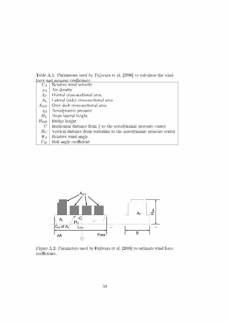
Table A.1: Parameters used by Fujiwara et al. [2006] to calculate the windforce and moment coe�cients.
UA Relative wind velocityρA Air densityAF Frontal cross-sectional areaAL Lateral (side) cross-sectional area
AOD Over deck cross-sectional areaqA Aerodynamic pressureHL Mean lateral height
HBR Bridge heightC Horizontal distance from G to the aerodynamic pressure center
HC Vertical distance from waterline to the aerodynamic pressure centerΨA Relative wind angleCH Roll angle coe�cient
Figure A.2: Parameters used by Fujiwara et al. [2006] to estimate wind forcecoe�cients.
53

= CLF cos ΨA + (A.5)
+ CXLI(sin ΨA − 1/2 sin ΨA cos2 ΨA) · sin ΨA cos ΨA ++ CALF sin ΨA cos3 ΨA
CAY (ΨA) = F ′CF + F ′Y LI
= CCF sin2 ΨA + (A.6)
+ CY LI(cos ΨA +12
sin2 ΨA cos ΨA) · sin ΨA cos ΨA
using the longitudinal-�ow drag, F ′LF , lift induced drag, F ′XLI , and addi-tional longitudinal drag, F ′ALF . For the lateral force coe�cient the cross-�owdrag, F ′CF , and the lift induced drag, F ′Y LI , in the lateral direction are used.
The roll angle coe�cient is calculated using
CH = 0.355φ+ 1.0 (A.7)
with the heel angle φ [rad].
Table A.2: Non-dimensional parameters for wind load estimation equationsi j: 0 1 2 3 4
αj 0.404 0.368 0.902
βij 1 -0.922 0.507 1.1622 0.018 -5.091 10.367 -3.011 -0.341
γij 1 0.116 3.3452 0.446 2.192
δij 1 0.458 3,245 -2.3132 -1.901 12.727 24.407 -40.310 -5.481
εij 1 -0.585 -0.906 3.2392 -0.314 -1.117
54

Using the values from table A.2 the cross-�ow and longitudinal-�ow co-e�cients are:
CCF = α0 + α1AF
BHBR+ α2
HBR
LOA(A.8)
C0◦6Ψ690◦
LF = β10 + β11AL
LOAB+ β12
C
LOA
C90◦6Ψ6180◦
LF = β20 + β21B
LOA+ β22
HC
LOA+
+ β23AODL2OA
+ β24AFB2
(A.9)
The lift and induced drag coe�cient in the term F ′Y LI :
CY LI = πALL2OA
+ CYM (A.10)
where the corrective term, CYM , a�ected from the ship hull form above sealevel separates into wind direction dependant coe�cients as follows:
C0◦6Ψ690◦
YM = γ10 + γ11AF
LOAB
C90◦6Ψ6180◦
YM = γ20 + γ21AODL2OA
(A.11)
The lift and induced drag coe�cients in the term F ′XLI :
C0◦6Ψ690◦
XLI = δ10 + δ11AL
LOAHBR+ δ12
AFBHBR
C90◦6Ψ6180◦
XLI = δ20 + δ21AL
LOAHBR+ δ22
AFAL
+ (A.12)
+ δ23B
LOA+ δ24
AFBHBR
The coe�cient CALF in the term F ′ALF :
C0◦6Ψ690◦
ALF = ε10 + ε11AODAL
+ ε12B
LOA
C90◦6Ψ6180◦
ALF = ε20 + ε21AODAL
(A.13)
The yaw and heel moment coe�cients are calculated using the lateralwind force coe�cient:
CAN (ΨA) = CAY (ΨA)LN (ΨA)
= CAY (ΨA)[0.927× C
LOA− 0.149× (ΨA −
π
2)]
(A.14)
55

CAK(ΨA) = CAY (ΨA)LK
= CAY (ΨA)(0.0737×( HC
LOA
)−0.821) for
HC
LOA6 0.097
= CAY (ΨA)(0.500) forHC
LOA> 0.097 (A.15)
56

Appendix B
Holtrop-Mennen
B.1 Resistance factor calculations
The total resistance of the ship is calculated according to:
Rhydro = RF (1 + k1) +RAPP +RW +RB +RTR +RA (B.1)
The frictional resistance is de�ned according to the ITTC-57 formula:
RF =12ρU2
SCFStot (B.2)
CF =0.075
(log10(Rn)− 2)2(B.3)
where ρ is the water density, US is the ships speed, CF frictional coe�cient,Stot is the total wetted surface area and Rn = USLν the Reynolds numberbased on waterline length L and kinematic viscosity ν of water.
For the form factor Holtrop [1984] suggests the following formula:
1 + k1 = 0.93 + 0.487118c14(B/L)1.06806(T/L)0.46106
(L/LR)0.121563(L3/5)0.36486(1− CP )−0.604247 (B.4)
here B is the molded breadth, T the molded depth, 5 the volume displace-ment and CP the prismatic coe�cient.
The coe�cient c14 pertains to the shape of the stern and is for all theships modeled equal to 1. LR is de�ned as:
LR = L(1− CP + 0.06CP lcb/(4CP − 1)) (B.5)
with lcb being the longitudinal position of the center of buoyancy forwardof G as percentage of L.
The wetted surface area of the ship can be approximated using, Holtropand Mennen [1982]:
Stot = L(2T +B)√CM (0.453 + 0.4425CB − · · ·
−0.2862CM − 0.003467B/T + 0.3696CWP ) + · · ·+2.38ABT /CB (B.6)
57

where CM is the amidships section coe�cient, CB the block coe�cient, CWP
the water plane area coe�cient and ABT the transverse sectional area forthe bulb at the forward perpendicular.
For the appendage resistance, RAPP , the same equation as B.2 can beused but with the appendage surface area, SAPP , instead of Stot and ap-pendage form factors (1 + k2) where Holtrop and Mennen [1982] provides(1 + k2) ≈ 1.7 for rudder behind skeg and (1 + k2) ≈ 1.4 for rudder behindstern.
The wave resistance, RW , is given by Holtrop [1984] for ships with Froudenumbers bellow 0.4 as:
RW = c1c2c6 5 ρgem1F dn+m4 cos(λF−2
n ) (B.7)
with:
c1 = 2223105c3.786137 (T/B)1.07961(90− iE)−1.37565 (B.8)
c7 = 0.229577(B/L)0.3333 when B/L < 0.11 (B.9)
c7 = B/L when 0.11 < B/L < 0.25 (B.10)
c7 = 0.5− 0.0625L/B when B/L > 0.25 (B.11)
c2 = e−1.89√c3 (B.12)
c3 = 0.56A1.5BT /{BT (0.31
√ABT + TF − hb}) (B.13)
c6 = (1− 0.8AT /(BTCM )) (B.14)
m1 = 0.0140407L/T − 1.7525451/3 /L− 4.79323B/L− c16 (B.15)
c16 = 8.07981CP − 13.8673C2P + 6.984388C3
P when CP < 0.8(B.16)c16 = 1.73012− 0.7067CP when CP > 0.8 (B.17)
d = −0.9 (B.18)
m4 = c150.4e−0.034F−3.29n (B.19)
c15 = −1.69385 when L3/5 < 512 (B.20)
c15 = −1.69385 + (L/51/3 −8)/2.36 (B.21)
when 512 < L3/5 < 1726.91c15 = 0 when L3/5 > 1726.91 (B.22)
λ = 1.446CP − 0.03L/B when L/B < 12 (B.23)
λ = 1.446CP − 0.36 when L/B > 12 (B.24)
where AT is the transverse area of the inversed transom at zero speed, hbthe center of the transverse area of the bulbous bow,ABT , above the keel lineand TF the forward draft.
The half angle of entrance iE is de�ned by Holtrop and Mennen [1982]between 1◦ to 90◦ as:
iE = 1 + 89exp{−(L/B)0.80856(1− CWP )0.30484
58

(1− CP − 0.0225lcb)0.6367(LR/B)0.34574
(1005 /L3)0.16302} (B.25)
For the resistance of a bulbous bow near the surface Holtrop and Mennen[1982] provide the following formula:
RB = 0.11e−3P−2B F 3
niA1.5BTρg/(1 + F 2
ni) (B.26)
where the emergence of the bow is measured by the coe�cient PB and theFroude number based on immersion, Fni:
PB = 0.56√ABT /(TF − 1.5hb) (B.27)
Fni = Us/
√g(TF − hb − 0.25
√ABT ) + 0.15U2
s (B.28)
Further the immerse transom produces an additional resistance as:
RTR = 0.5ρU2SAT c6 (B.29)
with c6 related to the Froude number based on the transom immersion FnT :
c6 = 0.2(1− 0.2FnT ) when FnT < 5 (B.30)
c6 = 0 when FnT > 5 (B.31)
FnT = US/√
2gAT /(B +BCWP ) (B.32)
where CWP is the water plane area coe�cient.In order to have a better congruence of results from model test to full
scale trials a model-ship correlation resistance RA is calculated by Holtropand Mennen [1982] as:
RA =12ρU2
SSCA (B.33)
with:
CA = 0.006(L+ 100)−0.16 − 0.00205 + · · ·+0.003
√L/7.5C4
Bc2(0.04− c4) (B.34)
c4 = TF /L when TF /L 6 0.04 (B.35)
c4 = 0.04 when TF /L > 0.04 (B.36)
CA is to be increased if another �gure of the standard roughness ks =150µm is used.
59

Appendix C
Propeller force calculations
C.1 Propeller non-dimensional coe�cients
Principles of Naval Architecture, Lewis [1988, p 145], uses the following non-dimensional coe�cients to describe a propeller advance ratio, J , thrust coef-�cient, KPT , and moment coe�cient, KQ as well as the propeller e�ciency,η0 according to:
J =UInD
(C.1)
KPT =FP
ρhn2D4(C.2)
KQ =Q
ρhn2D5(C.3)
η0 =J
2π× KT
KQ(C.4)
where KPT , KQ and η0 are functions of J . In equations C.1 to C.4 thevariables used are incident water speed at the propeller or advance speed,UI [m/s], rotational speed, n [rev/s], propeller diameter, D [m], thrust force,FP [N], propeller moment, Q [Nm], and water density, ρh [kg/m3]. Thecoe�cients presented here are read from open water curves produced forpropellers by Lindgren and Bjärne [1967] and presented in Garme [2007].
C.2 Taylor wake fraction, w
Propeller testing is done in an open con�guration where the incident wateris free from disturbances. When the propeller is placed behind the hull of aship the incident water is a�ected by the hull. One of the e�ects is that thewater behind the hull has been accelerated by the hull in the direction oftravel. This produces a wake behind the ship that makes the propeller workin water with a lower incidence speed, UI , than US . The di�erence between
60

the speeds is de�ned by the Taylor wake fraction, w, as presented in Lewis[1988, p 145-6]:
w =US − UIUS
→ (C.5)
→ UI = US(1− w) (C.6)
Several approximations of the wake fraction are presented in the litera-ture. Here the approximation for single screw ships by Tornblad [1990] ascitet by Garme [2007, eq. 61] is used:
w = 0.5CB − 0.05 (C.7)
C.3 Force calculation
The propeller force is calculated using equations C.1 and C.5 to derive acorrected advance ratio:
Jw =US(1− w)
Dn(C.8)
61

Appendix D
Data plots for selected states indatabase analysis
62

D.1 Crown, Number of data points
(a) 1-9 highest number of data points
(b) 10-18 highest number of data points
Figure D.1: Plots of the highest number of data points in each state forCrown class, Wind force 0-5 beaufort
63

TableD.1:
Crow
nclass
results
fornumber
ofcon
tainers
fromdatab
ase.Windforce
0-5beau
fort,lim
confint =
10.Wind
Wind
Mean
Mean
I95%
Coe�
cient
Number
ofMean
fuel
∆HFC/con
tainer
Direction
Force
speed
TFHC/con
tainer
data
poin
tcon
sumption
44
20,56
0,0146-0,0002296
1491,5523
-0,00014791
519,5
7,950,0102
8,39E-05
1381,6374
5,12E-05
24
19,57,95
0,0167-7,43E
-05133
1,6293-4,56E
-052
519,5
7,950,0152
-0,0002412132
1,6260-0,0001483
43
20,56
0,01460,0002516
1291,5630
0,00016092
320,5
60,0207
0,0001977116
1,56390,0001264
14
19,57,95
0,01320,0009477
1001,6448
0,00057614
419,5
60,0278
0,000231891
1,49800,0001547
23
19,57,95
0,02380,0006539
781,5873
0,00041194
520,5
60,0194
0,000262775
1,56460,0001679
23
20,57
0,0179-1,16E
-0573
1,5961-7,28E
-062
420,5
60,0213
-0,000174071
1,5630-0,0001113
24
19,57
0,01800,0005440
701,6008
0,000339824
420,5
70,0158
-0,000135870
1,5932-8,52E
-051
419,5
70,0186
0,000271669
1,61900,0001677
14
20,56
0,03420,0002651
671,6195
0,00016372
320,5
4,950,0246
-0,000557166
1,5226-0,0003659
13
20,56
0,0214-0,0002570
621,5982
-0,0001608
64
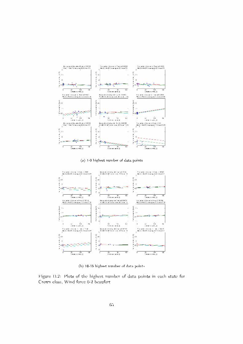
(a) 1-9 highest number of data points
(b) 10-18 highest number of data points
Figure D.2: Plots of the highest number of data points in each state forCrown class, Wind force 0-2 beaufort
65

D.2 Crown, I95%
(a) 1-9 smallest I95%
(b) 10-18 smallest I95%
Figure D.3: Plots of the states with the smallest con�dence interval I95% forCrown class, Wind force 0-5 beaufort
66
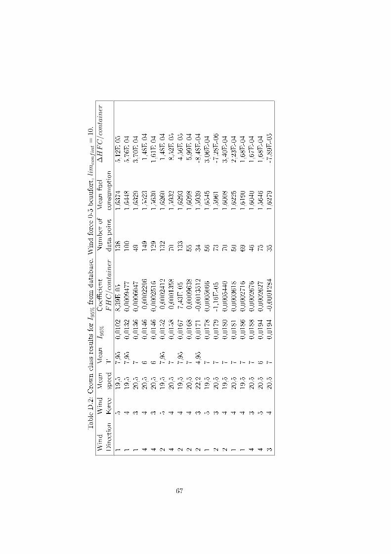
TableD.2:CrownclassresultsforI 9
5%from
database.
Windforce0-5beaufort,limconfint
=10.
Wind
Wind
Mean
Mean
I 95%
Coe�
cient
Number
ofMeanfuel
∆HFC/container
Direction
Force
speed
TFHC/container
datapoint
consumption
15
19,5
7,95
0,0102
8,39E-05
138
1,6374
5,12E-05
14
19,5
7,95
0,0132
0,0009477
100
1,6448
5,76E-04
13
20,5
70,0136
0,0006047
491,6329
3,70E-04
44
20,5
60,0146
-0,0002296
149
1,5523
-1,48E
-04
43
20,5
60,0146
0,0002516
129
1,5630
1,61E-04
25
19,5
7,95
0,0152
-0,0002412
132
1,6260
-1,48E
-04
44
20,5
70,0158
-0,0001358
701,5932
-8,52E
-05
24
19,5
7,95
0,0167
-7,43E
-05
133
1,6293
-4,56E
-05
24
20,5
70,0168
-0,0009638
551,6098
-5,99E
-04
23
22,2
4,95
0,0171
-0,0013512
341,5939
-8,48E
-04
15
19,5
70,0178
0,0005066
561,6545
3,06E-04
23
20,5
70,0179
-1,16E
-05
731,5961
-7,28E
-06
24
19,5
70,0180
0,0005440
701,6008
3,40E-04
14
20,5
70,0181
0,0003618
501,6225
2,23E-04
14
19,5
70,0186
0,0002716
691,6190
1,68E-04
43
20,5
70,0188
0,0002676
461,6040
1,67E-04
45
20,5
60,0194
0,0002627
751,5646
1,68E-04
34
20,5
70,0194
-0,0001284
351,6279
-7,89E
-05
67

(a) 1-9 smallest I95%
(b) 10-18 smallest I95%
Figure D.4: Plots of the states with the smallest con�dence interval I95% forCrown classs, Wind force 0-2 beaufort
68

D.3 Family, Number of data points
(a) 1-9 highest number of data points
(b) 10-18 highest number of data points
Figure D.5: Plots of the highest number of data points in each state forFamily class, Wind force 0-5 beaufort
69
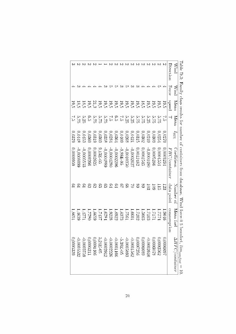
TableD.3:
Fam
ilyclass
results
fornumber
ofcon
tainers
fromdatab
ase.Windforce
0-5beau
fort,lim
confint =
10.Wind
Wind
Mean
Mean
I95%
Coe�
cient
Number
ofMean
fuel
∆HFC/con
tainer
Direction
Force
speed
TFHC/con
tainer
data
poin
tcon
sumption
24
19,57,5
0,02700,0003234
1231,9046
0,00016972
519,5
5,750,0254
0,0004554115
1,77740,0002562
24
19,55,75
0,03030,0005286
1091,7171
0,00030782
419,5
5,250,0249
-0,0004480103
1,7163-0,0002610
24
18,55,75
0,03020,0002545
891,5063
0,00016892
319,5
5,750,0315
0,001248289
1,72020,0007256
23
19,55,25
0,0421-0,0002627
701,6601
-0,00015822
519,5
5,250,0268
-0,001035068
1,7561-0,0005893
23
19,57,5
0,0409-9,88E
-0567
1,8373-5,38E
-052
519,5
6,50,0364
-0,000220664
1,8922-0,0001166
25
19,57,5
0,0284-0,0004280
641,9228
-0,00022261
319,5
5,750,0358
-0,000488963
1,6784-0,0002912
14
19,55,75
0,03039,13E
-0563
1,74375,24E
-052
421,3
5,750,0319
0,000262562
1,86590,0001406
24
19,56,5
0,03600,0009266
621,7780
0,00052112
418,5
5,250,0453
-0,000555361
1,4771-0,0003759
23
18,55,75
0,0448-0,0008099
611,4639
-0,00055323
419,5
7,50,0379
0,000995961
1,86510,0005339
70
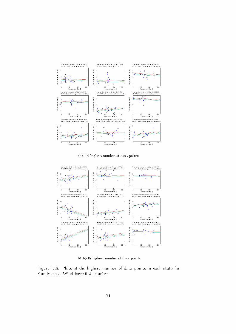
(a) 1-9 highest number of data points
(b) 10-18 highest number of data points
Figure D.6: Plots of the highest number of data points in each state forFamily class, Wind force 0-2 beaufort
71

TableD.4:
Fam
ilyclass
results
fornumber
ofcon
tainers
fromdatab
ase.Windforce
0-2beau
fort,lim
confint =
10.Wind
Wind
Mean
Mean
I95%
Coe�
cient
Number
ofMean
fuel
∆HFC/con
tainer
Direction
Force
speed
TFHC/con
tainer
data
poin
tcon
sumption
12
177.5
0.0506-0.0004202
351.2959
-0.00032432
217
5.250.0670
-0.000313031
1.2025-0.0002603
22
19.55.25
0.0541-0.0007047
301.7130
-0.00041142
219.5
5.750.0533
0.000398629
1.70900.0002332
12
175.25
0.04680.0011572
281.0754
0.00107612
219.5
7.50.0475
-0.000697928
1.9429-0.0003592
12
175.75
0.05920.0009683
271.2510
0.00077402
218.5
5.750.0616
-0.000193626
1.4585-0.0001327
12
18.55.25
0.06040.0012285
251.3617
0.00090221
218.5
7.50.0642
0.002064025
1.62330.0012715
12
19.57.5
0.0590-0.0005191
251.8622
-0.00027882
221.3
5.750.0279
-0.000184024
1.8423-0.0000999
12
176.5
0.0717-0.0049939
241.3162
-0.00379431
117
5.250.0475
0.001345223
1.07110.0012558
12
19.55.75
0.05260.0010857
231.7533
0.00061931
117
7.50.0633
0.005310522
1.30640.0040651
22
177.5
0.09070.0018113
221.3781
0.00131444
221.3
5.250.0484
-0.000163221
1.8090-0.0000902
72

D.4 Family, I95%
(a) 1-9 smallest I95%
(b) 10-18 smallest I95%
Figure D.7: Plots of the states with the smallest con�dence interval I95% forFamily class, Wind force 0-5 beaufort
73
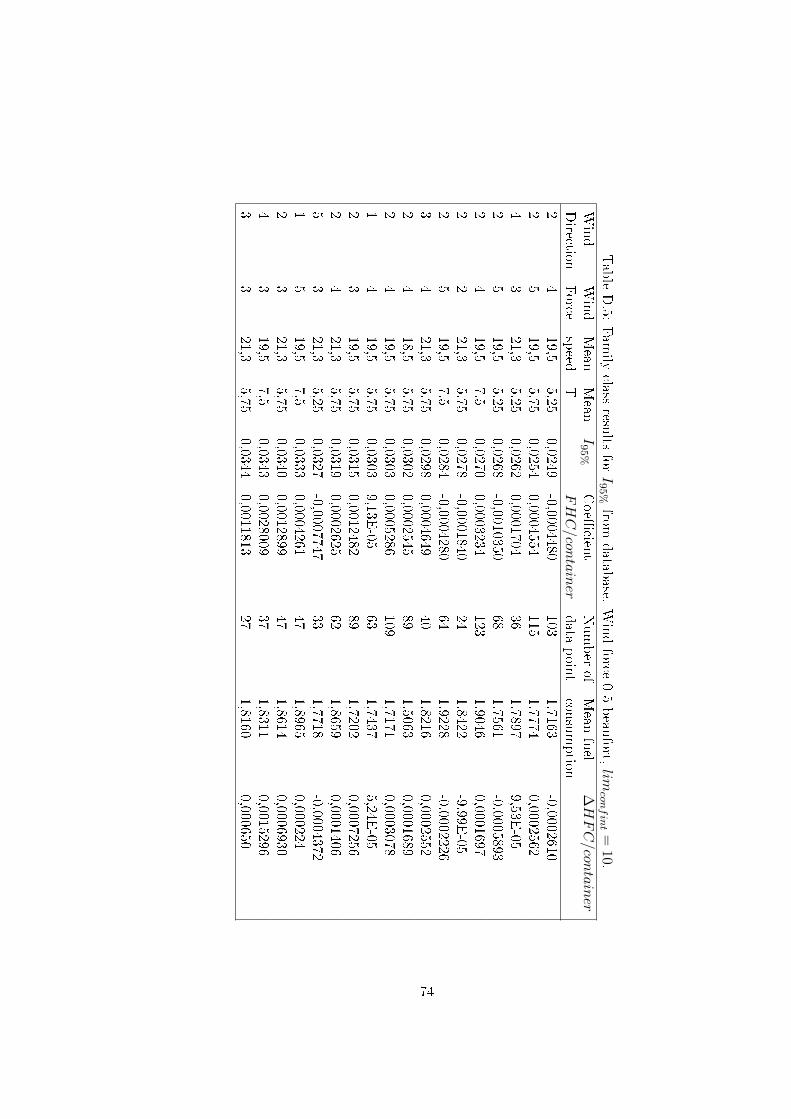
TableD.5:
Fam
ilyclass
results
forI
95%from
datab
ase.Windforce
0-5beau
fort,lim
confint =
10.Wind
Wind
Mean
Mean
I95%
Coe�
cient
Number
ofMean
fuel
∆HFC/con
tainer
Direction
Force
speed
TFHC/con
tainer
data
poin
tcon
sumption
24
19,55,25
0,0249-0,0004480
1031,7163
-0,00026102
519,5
5,750,0254
0,0004554115
1,77740,0002562
43
21,35,25
0,02620,0001704
361,7897
9,53E-05
25
19,55,25
0,0268-0,0010350
681,7561
-0,00058932
419,5
7,50,0270
0,0003234123
1,90460,0001697
22
21,35,75
0,0278-0,0001840
241,8422
-9,99E-05
25
19,57,5
0,0284-0,0004280
641,9228
-0,00022263
421,3
5,750,0298
0,000464940
1,82160,0002552
24
18,55,75
0,03020,0002545
891,5063
0,00016892
419,5
5,750,0303
0,0005286109
1,71710,0003078
14
19,55,75
0,03039,13E
-0563
1,74375,24E
-052
319,5
5,750,0315
0,001248289
1,72020,0007256
24
21,35,75
0,03190,0002625
621,8659
0,00014065
321,3
5,250,0327
-0,000774733
1,7718-0,0004372
15
19,57,5
0,03330,0004261
471,8965
0,0002242
321,3
5,750,0340
0,001289947
1,86140,0006930
43
19,57,5
0,03430,0028009
371,8311
0,00152963
321,3
5,750,0344
0,001181327
1,81600,000650
74

(a) 1-9 smallest I95%
(b) 10-18 smallest I95%
Figure D.8: Plots of the states with the smallest con�dence interval I95% forFamily classs, Wind force 0-2 beaufort
75

TableD.6:
Fam
ilyclass
results
forI
95%from
datab
ase.Windforce
0-2beau
fort,lim
confint =
10.Wind
Wind
Mean
Mean
I95%
Coe�
cient
Number
ofMean
fuel
∆HFC/con
tainer
Direction
Force
speed
TFHC/con
tainer
data
poin
tcon
sumption
22
21.35.75
0.0279-0.0001840
241.8423
-0.00009994
221.3
5.750.0376
0.000576311
1.76390.0003267
22
19.56.5
0.04070.0007142
171.8203
0.00039244
217
5.250.0448
0.001505416
1.03930.0014486
12
175.25
0.04680.0011572
281.0754
0.00107612
219.5
7.50.0475
-0.000697928
1.9429-0.0003592
11
175.25
0.04750.0013452
231.0711
0.00125584
221.3
5.250.0484
-0.000163221
1.8090-0.0000902
12
177.5
0.0506-0.0004202
351.2959
-0.00032435
218.5
5.250.0506
0.002233112
1.27430.0017525
11
21.35.75
0.05090.0032136
101.9483
0.00164941
219.5
5.750.0526
0.001085723
1.75330.0006193
12
19.55.25
0.05280.0012169
201.5948
0.00076312
219.5
5.750.0533
0.000398629
1.70900.0002332
22
19.55.25
0.0541-0.0007047
301.7130
-0.00041143
219.5
5.750.0578
0.001481613
1.63890.0009040
32
19.57.5
0.05840.00317616
181.9352
0.00164131
219.5
7.50.0590
-0.000519125
1.8622-0.0002788
76

D.5 Spread of I95%
The spread of I95% can here seen as well as the detailed spread above the cho-sen lower limit for the number of data points used in the selection accordingto I95%.
(a) Wind force 0-5 beaufort. Lower limit 10 data points
(b) Wind force 0-2 beaufort. Lower limit 5 data points
Figure D.9: Spread of I95% for Crown class
77

(a) Wind force 0-5 beaufort. Lower limit 10 data points
(b) Wind force 0-2 beaufort. Lower limit 10 data points
Figure D.10: Spread of I95% for Family class
78