When and Where: Deep diving into Wireless...

When and Where: Deep diving into Wireless Localization

Dr. Domenico Giustiniano

Computer Engineering and Networks Laboratory (TIK)Communication Systems Group (CSG)

Introduction

Localize me!

This class covers the system designs and trade-offs of pervasive positioningmethods and their underlying technologies, focusing on mobile positioning.

D. Giustiniano When and Where

Introduction

What application?

Location is at the core of a number of high-value Location-Based Services(LBS) on smarthphones:

navigation, social applications, emergency response, advertisements,sport.

E.g. Social check-in (Foursquare), Friends-find APP (Google Latitude)

key for emerging applications

personalized experiences in games and theme parksaugmented reality.


Introduction

Once upon a time...(I)

In 1998, the FCC rolled out phase I of E911:

carriers should identify the originating call’s phone number andthe location of the cell tower, accurate to within a mile.

(Automatic Location Identification (ALI)).

In 2001, the FCC rolled out phase 2 of E911

FCC required that each carrier in the US must detect the caller’slocation within 100 meter accuracy.GPS was not an option at that time.


Introduction

Once upon a time...(II)

LBS were initially launched in Japan:

July 2001: Docomo → pre-GPS handsets.December 2001: KDDI → first mobile phones with GPS.

1st mobile LBS search application launched by AT&T in May 2002

It used ALI.

The users were able to use ALI to:

determine their locationfind list of search query results near their location

(restaurants, hospitals, etc.).


Introduction

Market Growth

Two main key success factors:growing adoption of GPS devices and smartphone adoption.


Introduction

LBS APPs

source: “http://www.skyhookwireless.com/locationapps/”


Introduction

LBS by Category


http://www.skyhookwireless.com/locationapps/

Introduction

Paid versus Free LBS


Introduction

Where am I? What’s around me?

Example: MyLocation from Google (Maps)

Available for outdoor navigation, and partially for indoor navigation.

Adding new indoor maps to public buildings across the world.

In Switzerland, already available in some locations, including:

Sihlcity (Zurich)Airport Center, Zurich Airport


Introduction

Absolute location

Our focus is to determine the absolute location. We distinguish:

Positioning, estimation of the position.

Navigation, where besides the position, also velocity, heading,acceleration and angular rates are estimated

Target tracking, where another object’s position is to be estimatedbased on measurements of relative range and angles.


Introduction

Main technologies

Positioning technologies of mobile devices fall in three main categories:

1 GNSS (Global Navigation Satellite System)

2 Network-based positioning systems (Cellular, Wi-Fi, Bluetooth, ...)

3 Inertial tracking systems


Metrics

Metrics


Metrics

Metrics: Accuracy

The most important requirement of positioning systems.

Performance metric: mean distance error E [e]

For each sample: Euclidean distance e between the estimated locationp =

(x , y , z

)and the true location p =

(x , y , z

).

Accuracy

E [e] = E [‖p − p‖] = E [√(

x − x)2

+(y − y

)2+(z − z

)2]


Metrics

Accuracy of GPS, WPS and GSM

In tests with clear view of sky:

GPS is more accurate than WPSWPS=WiFi-based positioning system from Skyhook.

GSM-based positioning has an error as high as 300 m.

source: “Energy-efficient rate-adaptive GPS-based positioning for smarthphones”, Mobisys 2010


Metrics

GPS in urban areas



Metrics

Accuracy of GPS versus ground truth



Metrics

Example using Android Wingle APP and Google Fusion


Metrics

Metrics: Precision

The precision considersalso the CDF distribution

“Empirical evaluation of the limits on localization using signal strength”, SECON’09


Metrics

Cost

Computation Cost

Minimise it when location is calculated on mobile devices.Some units (as passive RFID tags) are completely energy passive.

Hardware Cost

Mobile units may have tight space and weight constraints.A positioning system that uses a technology already for communicationdoes not have hardware cost.


Metrics

Other metrics

Power Consumption

Keeping GPS activated continuously would drain the battery on asmartphone in less than 6− 11 hours.

Response time

it should be sufficiently fast to allow to track mobile targets.

Required infrastructure

none, markers, passive tags, active beacons, pre-existing or dedicated,local or global.

Coverage area

single room, building, city, global.


Metrics

Pinpoint position?

Accuracy (m)

Response time (ms)

Power Consumption (mW)

Figure: Kiviat diagram

No single location technology exhibits high accuracy, low response time,low consumption, low cost and universal coverage for every situation.


Technologies: GPS

Technologies: GPS


Technologies: GPS Principles of GPS

What is GPS?

The Global Positioning System (GPS) is a satellite-based navigationsystem

made up of a network of 24 satellites placed into orbit between 1978and 1994 by US.

GPS satellites send signals for civilian use at the 1.575 Ghz frequency.

Satellites are positioned so that every location of the earth’s surfacehas access to four satellites 24 h a day.

Satellites orbit the earth in 12 hours.

33 satellites in orbit as of March 2008.

A set of ground stations monitor the satellites’ trajectory and health,and send the satellite parameters to the satellites.



source: “http://www.n2yo.com/”



GPS signal modulation (I)

Carrier modulated with a Pseudo-Random Noise (PRN) code

unique to each satellite.37 suitable codes (GOLD codes).

Code multiplexing: PRN allows to use a single receiver for receivingthe signal of multiple satellites.



GPS signal modulation (II)

Modulated additionally with a navigation message

with almanac data and its precise ephemeris data.



Navigation data

A full data packet from a satellite broadcast is 30 sec long, containing 5six-second-long frames.

Ephemeris data are the orbit parameters for the satellite andsatellite’s predicted trajectory as a function of time.Almanac data consists of coarse orbit and status information for eachsatellite in the constellation.

Used for easier acquisition of further satellites.


http://www.n2yo.com/


How the receiver calculates its position (I)

Each GPS satellite has an on-board atomic clock and includes thetimestamp [time sent] of the signal it broadcasts (HOW).

GPS signals take from 64 to 89 ms to travel from a satellite to theEarth’s surface.

The receiver decodes the satellite timestamp, and hence it knowswhen the signal was transmitted.

A GPS receiver also keeps track of time (with its clock) of thereceived signal [time received].



How the receiver calculates its position (II)

Coarse estimation:Compute tp by using [time sent] and [time received] at packet level.

Accuracy is in the order of ms.

Fine estimation:Compute the sub-millisecond part of tp at PRN code level, measuringthe time shift tp between the local copy and received PRN code.

Figure from P. Steemkiste, CMU



How the receiver calculates its position (III)

A GPS receiver acquires each GPS satellite’s signal by correlating thesignal it receives with a local copy of the satellite’s PRN code.

Acquisition requires shifting the copy both in time (distance) andfrequency (Doppler effect).

source: “Energy Efficient GPS Sensing with Cloud Offloading”, Sensys 2012



How the receiver calculates its position (IV)

d = ctp: Speed of light is known, and hence the distance from eachsatellite to the receiver (called pseudoranges) is estimated.

Trilateration algorithms are finally applied to calculate the position ofthe GPS receiver.



Cold and Hot Start

Time-To-First-Fix (TTFF)

Time required for a GPS receiver to acquire satellite signals and navigationdata, and calculate its position.

Cold start is the TTFF, while starting without initial position, time,almanac and ephemeris.

50− 300 sec

Warm start, when the receiver has a previous lock to the satellites, itcan start from the previous Doppler shift and code phases.

Hot start is the TTFF starting with initial position, time, almanacand ephemeris.

4− 30 sec

50 bps data rate explains why a standalone GPS takes some time for TTFF



Assisted GPS (A-GPS)

A-GPS allows for hot start by sending almanac and ephemeris datavia an additional communication channel to a GPS receiver

e.g. using a cellular network or WiFi.

After a hot start, TTFF depends on how fast a GPS receiver can tuneto the carrier frequencies (shifted due to Doppler effect) andsyncronize with their signals.

It is in the order of tens of sec when target moves, less when it is static.

However, it does not improve positioning accuracy.



Real-time differential GPS

Using commercial off-the-shelf hardware: precision of 7.8 m in 95%

due to systematic and nonsystematic errors.

Differential methods or military GPS receivers can minimize some ofthe systematic errors

accuracy up to 0.3 m.

They correct bias errors at one location with measured bias errors ata known position

Tower or satellite (Wide Area Augmentation System (WAAS).

However Differential GPS is quite expensive.



Trilateration algorithms



Range-based schemes

Triangulation = working with angles

Measuring the angle with respect to reference points and a referencedirection.

Those angles determine rays.

Their intersection gives the triangulation point.

Trilateration = working with distances

Measuring distances to reference points.

They intersect in the trilateration points.

GPS uses trilateration!



Basic notions of trilateration

Lateration is the most common method for deriving the location of awireless device.

For example, GPS uses trilateration.

Two steps are involved: ranging and lateration.1 The distance (range) to the anchors is calculated.2 The location of the wireless device is estimated based on these

distances.



GPS Time-of-Flight

The (xi , yi , zi ) components of i-th satellite position and the time sentare (xi , yi , zi , ti ).

The message traveled at the speed of light c .

It reaches the destination at time tr ,

The distance traveled is (tr + b − ti )c .

b = bc represents the clock bias b [µs] of receiver in terms of distance.



Pseudorange

Pseudorange equation

ρi = ||si − p||+ b + v

ρi is measured for each satellite i .

si and p are the position of the i-th satellite and receiver.

v is the pseudorange measurement noise,

modeled as white noise.

b solved along with the position of the receiver.



One, two, three, four satellites: the GPS case

Figure from P. Steemkiste, CMU



Log example

12 10 10 8 35 40.0000000 0 11G21G31G29G12S26G 2G24G14G30G10S24

24574152.706 -444467.323 4727.657 43.000

21467975.296 -292886.318 3094.940 38.000

20093222.765 -184619.4132 1943.763 33.000

22340274.564 111703.3453 -1188.122 29.000

37651336.056 -125084.9782 1334.439 34.000

22827576.606 11482.5643 -138.480 29.000

20880239.835 -161500.549 1694.054 37.000

24004670.329 160075.6813 -1697.439 26.000

24636015.072 -462005.7093 4914.218 28.000

25127098.314 -221143.4543 2326.690 28.000

37391651.426 -120954.5962 1269.244 35.000


Technologies: GPS Data fitting

Data fitting



Main algorithms for trilateration positioning

The most used approaches for trilateration positioning:

Non-Linear Least Square (NLS).Bayes filters such as Extended Kalman filtering (EKF) methods.

There are 4 unknowns:

the coordinate of receiver position and the clock bias.

NLS is largely used to calculate these unknowns.

EKF for tracking and sensor fusion.



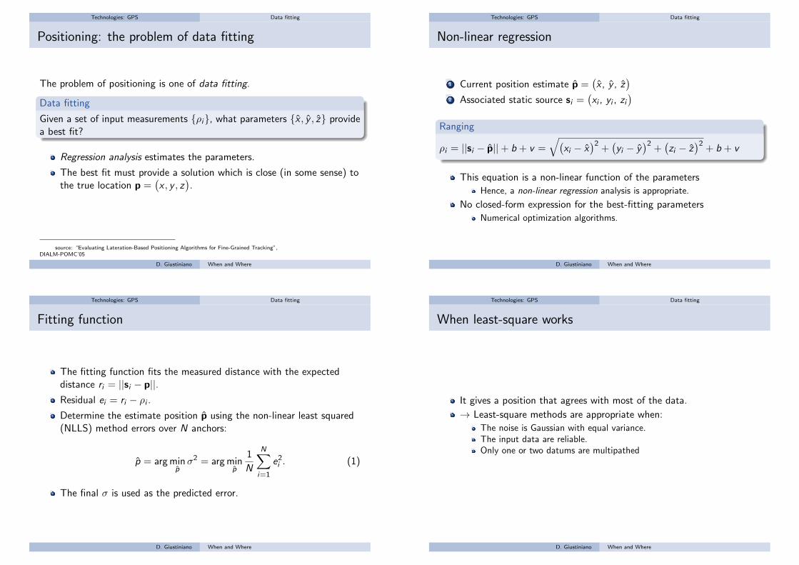
Positioning: the problem of data fitting

The problem of positioning is one of data fitting.

Data fitting

Given a set of input measurements {ρi}, what parameters {x , y , z} providea best fit?

Regression analysis estimates the parameters.

The best fit must provide a solution which is close (in some sense) tothe true location p =

(x , y , z

).

source: “Evaluating Lateration-Based Positioning Algorithms for Fine-Grained Tracking”,DIALM-POMC’05



Non-linear regression

1 Current position estimate p =(x , y , z

)2 Associated static source si =

(xi , yi , zi

)Ranging

ρi = ||si − p||+ b + v =√(

xi − x)2

+(yi − y

)2+(zi − z

)2+ b + v

This equation is a non-linear function of the parameters

Hence, a non-linear regression analysis is appropriate.

No closed-form expression for the best-fitting parameters

Numerical optimization algorithms.



Fitting function

The fitting function fits the measured distance with the expecteddistance ri = ||si − p||.Residual ei = ri − ρi .Determine the estimate position p using the non-linear least squared(NLLS) method errors over N anchors:

p = arg minpσ2 = arg min

p

1

N

N∑i=1

e2i . (1)

The final σ is used as the predicted error.



When least-square works

It gives a position that agrees with most of the data.

→ Least-square methods are appropriate when:

The noise is Gaussian with equal variance.The input data are reliable.Only one or two datums are multipathed



Why is multipath a problem?

Multipath causes a positive bias in the estimate distance

An over-estimation of the actual distance to the source.

Solutions:

PHY processing can alleviate severe multipath effects.data fitting function sufficiently robust to multipath.

NLOS

LOS

d2 > d1

d1



INLR

Iterative NLR (INLR) repeatedly remove outliers

(measurement with the greatest residual).

It computes a new non-linear model computed using the remainingdata.

Iterative process until fit (value σ) is good enough.

INLR gets better accuracy (and good multipath rejection) but it iscomputationally expensive.



Linearization: LLS algorithm

The Linear Least Square (LLS) approach linearizes the NLS problem,

by introducing a constraint in the formulation

It obtains a closed form expression of the estimated location.

“Handbook of Position Location: Theory, Practice, and Advances - Chap. 12: On the Performance ofWireless Indoor Localization Using Received Signal Strength”, Wiley Library



Starting with the N ≥ 2 equations to estimate the position (x , y):(x1 − x)2 + (y1 − y)2 = d2

1

(x2 − x)2 + (y2 − y)2 = d22

...

(xN − x)2 + (yN − y)2 = d2N

(2)

and subtracting the constraint

1

N

N∑i=1

[(xi − x)2 + (yi − y)2] =1

N

N∑i=1

d2i

from both sides of each equation, the above can be rewritten as Ap = b.



LLS

A =

x1 − 1

N

∑Ni=1 xi y1 − 1

N

∑Ni=1 yi

......

xN − 1N

∑Ni=1 xi yN − 1

N

∑Ni=1 yi

(3)



LLS

b =1

2

(x21 − 1

N

∑Ni=1 x2

i ) + (y 21 − 1

N

∑Ni=1 y 2

i )

−(d21 − 1

N

∑Ni=1 d2

i )

...

(x2N −

1N

∑Ni=1 x2

i ) + (y 2N −

1N

∑Ni=1 d2

i )

−(d2N −

1N

∑Ni=1 d2

i )

(4)

A only function of anchors’ coordinates.

b function of distances to anchors together with anchors’ coordinates.

p = (ATA)−1ATb



Pros and Cons of LLS algorithm

LLS is popular for ease of implementation.

It is highly susceptible to outliers.

LLS solution can serve as the starting point for the nonlinear leastsquares problem.

source: “Evaluating Lateration-Based Positioning Algorithms for Fine-Grained Tracking”,DIALM-POMC’05


Technologies: GPS Extended Kalman filter

Extended Kalman filter



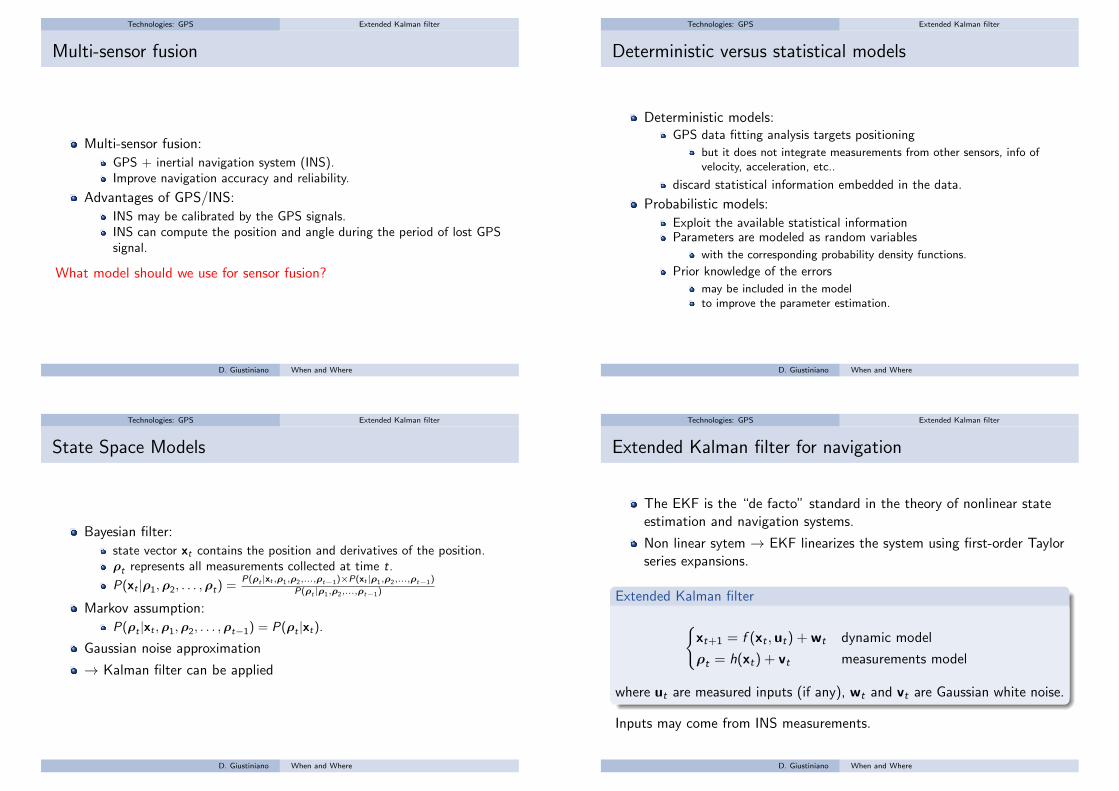
Multi-sensor fusion

Multi-sensor fusion:

GPS + inertial navigation system (INS).Improve navigation accuracy and reliability.

Advantages of GPS/INS:

INS may be calibrated by the GPS signals.INS can compute the position and angle during the period of lost GPSsignal.

What model should we use for sensor fusion?



Deterministic versus statistical models

Deterministic models:GPS data fitting analysis targets positioning

but it does not integrate measurements from other sensors, info ofvelocity, acceleration, etc..

discard statistical information embedded in the data.

Probabilistic models:

Exploit the available statistical informationParameters are modeled as random variables

with the corresponding probability density functions.

Prior knowledge of the errors

may be included in the modelto improve the parameter estimation.



State Space Models

Bayesian filter:

state vector xt contains the position and derivatives of the position.ρt represents all measurements collected at time t.

P(xt |ρ1,ρ2, . . . ,ρt) =P(ρt |xt ,ρ1,ρ2,...,ρt−1)×P(xt |ρ1,ρ2,...,ρt−1)

P(ρt |ρ1,ρ2,...,ρt−1)

Markov assumption:

P(ρt |xt ,ρ1,ρ2, . . . ,ρt−1) = P(ρt |xt).

Gaussian noise approximation

→ Kalman filter can be applied



Extended Kalman filter for navigation

The EKF is the “de facto” standard in the theory of nonlinear stateestimation and navigation systems.

Non linear sytem → EKF linearizes the system using first-order Taylorseries expansions.

Extended Kalman filter

{xt+1 = f (xt ,ut) + wt dynamic model

ρt = h(xt) + vt measurements model

where ut are measured inputs (if any), wt and vt are Gaussian white noise.

Inputs may come from INS measurements.



Design of Kalman filter for navigation

Dynamic model: linear.

Measurement model: non-linear.

(cartesian coordinates).

To achieve good filtering results:

Complete a priori knowledge of both the dynamic model andmeasurement model.Both the dynamic and the measurements are corrupted by zero-meanGaussian white noise.Initial estimate of the state is correct.The errors is within the “linear region”

accurate sensors or sensors with high update ratescovariance doesn’t propagated through linearization



State vector

We denote:

vt = [vx ,t vy ,t vz,t ]T as the receiver’s velocity.

b [m] and d [m/s] as the clock bias and clock drift.

If the velocity vt is measurable → xt = [xt yt zt b d ]T .



Dynamic and measurement model

Dynamic Model

For a sampling period Ts , the discrete time model f (xt) is:

f (xt) =

pt + Tsvt

b + Tsd

d

(5)

Masurement model

Using the pseudorange equation: h(xt) = ||si ,t − pt ||+ b



Linearization

Functions f (xt) and h(xt) are linearized to get the state transition matrixF and the measurement matrix H of an ordinary Kalman filter.

Linearization

xp = f (xt) provides linearization point (and predicted state estimate).

F = dfdxt

∣∣xp

linearizes the state equation.

H = dhdxt

∣∣xp

linearizes the measurement equation.model).

The filter then updates the state, as a normal Kalman filter:xo = xp + Kt(ρt − h(xp)), where Kt is the Kalman gain.



Example using Matlab script, with logs of pseudorange and satellites’position


Technologies: GPS GPS error

GPS error



GDOP: Geometric Dilution of Precision (I)

It measures how correlated are the pseudorange information:

GDOP =∆OutputLocation

∆MeasuredData.

It is a measure based solely on:the geometry of the satellitesclock-related components of the navigation solution.

(a) Low GDOP (b) High GDOP

source: “Dilution of Precision”, GPS World, 1999



GDOP: Geometric Dilution of Precision (II)

Ideally small changes in the measured data will not result in largechanges in output location.

When visible GPS satellites are close together in the sky, thegeometry is weak and the GDOP value is high.

When far apart, the geometry is strong and the DOP value is low(ideally DOP = 1).



HDOP

GDOP is often divided up into components Horizontal DOP (HDOP)and Vertical DOP (VDOP).

These componets are used because the accuracy of the GPS systemmay vary with the component.For example horizontal position can usually be measured moreaccurately than vertical position.

An HDOP of 6 or less → location error less than 12 m.

source: “Energy-Accuracy Aware Localization for Mobile Devices”, Mobisys 2010



GPS error in smarthphones (I)

The horizonal position error of GPS eGPS is:

eGPS =√

e2xGPS + e2

yGPS

exGPS and eyGPS are random variables that give the error in longitudeand latitute and have a normal distribution with zero mean.σrms =

√σ2xGPS + σ2

yGPS is the root mean square (RMS).

Assuming the same variance σ2 in both directions:

eGPS is Rayleigh distributed:

Pr (eGPS < r) = 1− exp

(− r 2

2σ2

)= 1− exp

(− r 2

σ2rms

)

“GPS/Galileo testbed using a high precision optical positioning systems”, SIMPAR ’10 and“Performance of collaborative GPS localization in pedestrian ad hoc networks”, Mobiopp ’12



GPS error in smarthphones (II)

When r = σrms , Pr (eGPS < σrms) ≈ 0.63.

Hence 63% of the errors fall within a circle of radius σrms .

σrms is referred as distance root-mean-square (dRMS).

Value that most GPS receivers report as their localization error.

Other receivers report 2dRMS,

r = 2σrms ,where 98% of the errors fall.



dRMS and HDOP

HDOP =

√σ2x+σ2

y

σ2r

= dRMSσr→ dRMS = σr · HDOP

where σ2r is the variance of pseudorange observations.

E [eGPS ] (accuracy) can be estimated from the error reported by GPSreceivers.

For Rayleigh distribution:

E [eGPS ] = σ√

π2 = dRMS

√π

2 .


Technologies: GPS GPS sensitivity

GPS sensitivity



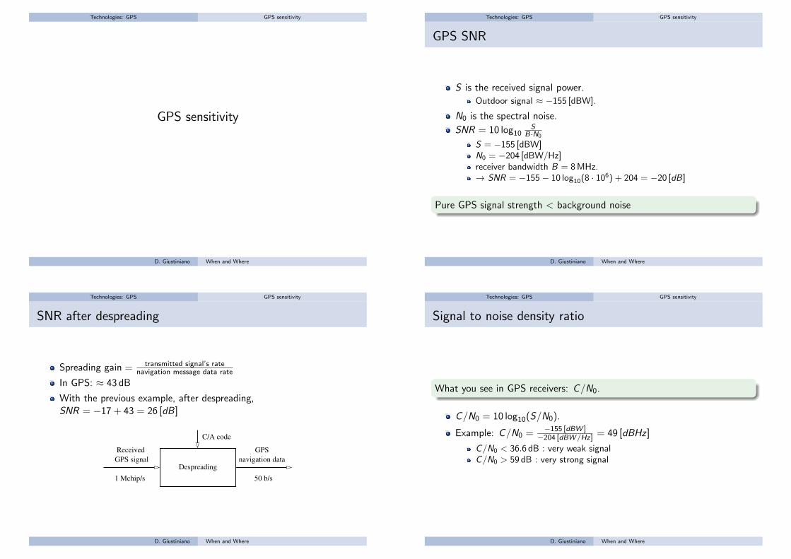
GPS SNR

S is the received signal power.

Outdoor signal ≈ −155 [dBW].

N0 is the spectral noise.

SNR = 10 log10S

B·N0

S = −155 [dBW]N0 = −204 [dBW/Hz]receiver bandwidth B = 8 MHz.→ SNR = −155− 10 log10(8 · 106) + 204 = −20 [dB]

Pure GPS signal strength < background noise



SNR after despreading

Spreading gain = transmitted signal’s ratenavigation message data rate

In GPS: ≈ 43 dB

With the previous example, after despreading,SNR = −17 + 43 = 26 [dB]

Despreading

C/A code

Received

GPS signal navigation data

GPS

50 b/s1 Mchip/s



Signal to noise density ratio

What you see in GPS receivers: C/N0.

C/N0 = 10 log10(S/N0).

Example: C/N0 = −155 [dBW ]−204 [dBW /Hz] = 49 [dBHz ]

C/N0 < 36.6 dB : very weak signalC/N0 > 59 dB : very strong signal



GPS indoor

GPS doesn’t provide pervasive coverage

But this situation may change due to

high-sensitivity receivers (HSGPS).Galileo system.

GPS sensitivity for HSGPS:

−190 dBW for tracking.−175 dBW for acquisition.



Precision of HSGPS with hot-start

But (not shown here) lower accuracy with cold start (or not sync at all)and TTFF from a few seconds to minutes.

Source: “Indoor Position using GPS revisited”, Pervasive 2010


Pervasive localization




Towards pervasive positioning system

How can we improve the accuracy, time response, coverage, etc. of ourpositioning system?

GPS is aided by other technologies.

Let’s look at the principles that make them complementary to GPS!


Pervasive localization Technologies: Inertial Tracking

Technologies: Inertial Tracking



Inertial Tracking

Use electronic accelerometers, compasses, and altimeters.

Sense movement and direction in 2D and 3D.

dead-reckoning → relative positions

(w.r.t. given fixed point).

position error grows with time and distance in the absence of:

position fixesfusion with other sensorscontext information (e.g., map)

Outdoor, but not indoorGPS is unreliable indoors,

rendering dead-reckoning based approaches useless.



Example

Positioning error can reach 5% of the distance travelled, in favorableconditions even 1% to 2%.

Source: “In Step with INS”, GPS World Magazine 2002



Accelerometer

An accelerometer measures all accelerations.

except those accelerations due to gravity.

An accelerometer indicates:

≈ 1g upwards, when at rest relative to the Earth’s surface.0g, during any type of free fall in a vacuum.



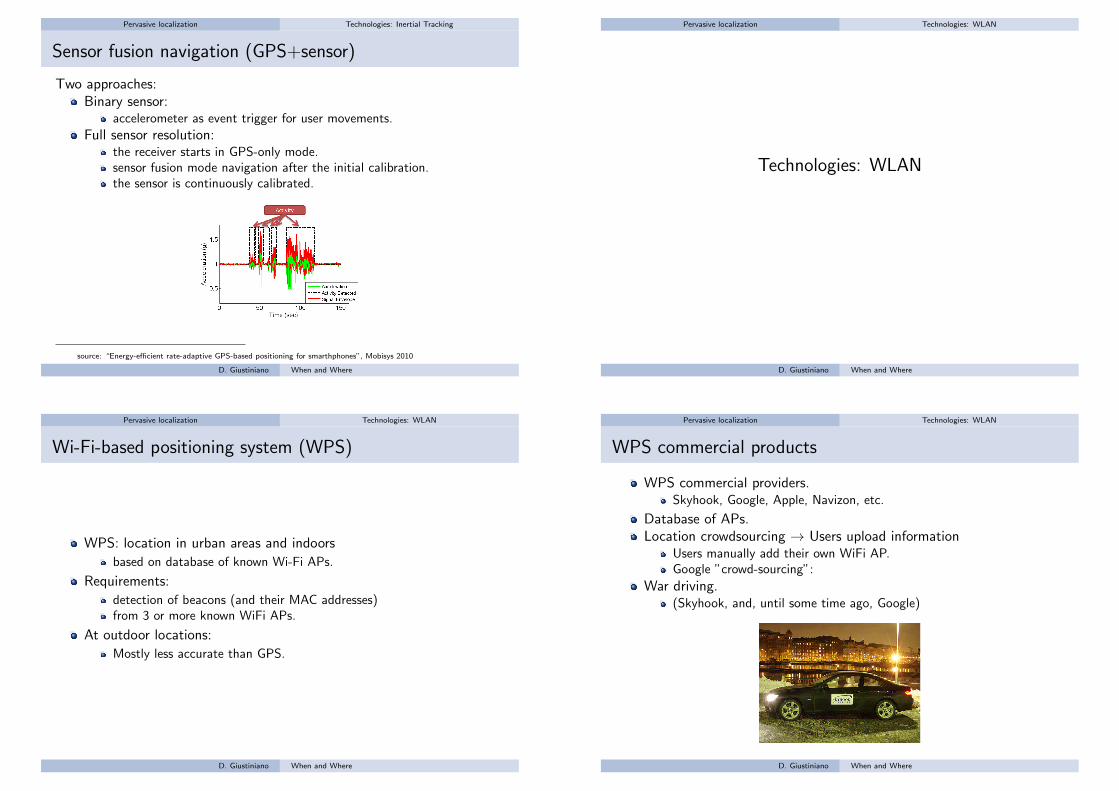
Sensor fusion navigation (GPS+sensor)

Two approaches:Binary sensor:

accelerometer as event trigger for user movements.

Full sensor resolution:the receiver starts in GPS-only mode.sensor fusion mode navigation after the initial calibration.the sensor is continuously calibrated.



Pervasive localization Technologies: WLAN

Technologies: WLAN



Wi-Fi-based positioning system (WPS)

WPS: location in urban areas and indoors

based on database of known Wi-Fi APs.

Requirements:

detection of beacons (and their MAC addresses)from 3 or more known WiFi APs.

At outdoor locations:

Mostly less accurate than GPS.



WPS commercial products

WPS commercial providers.Skyhook, Google, Apple, Navizon, etc.

Database of APs.Location crowdsourcing → Users upload information

Users manually add their own WiFi AP.Google ”crowd-sourcing”:

War driving.(Skyhook, and, until some time ago, Google)



Wingle WarDriving

Free database.

Over 74 million network beacons seen.

What happened after Jan-Mar 2010?!?



Key Hindrances

It requires a lot of hotspots.Mobile hotspots (Tethering mode).High dependence on Internet connectivity.Bad when moving fast (i.e. driving).Location database must be dynamically updated

to capture changing AP positions (everyday?).


Pervasive localization Technologies: Cell Tower

Technologies: Cell Tower



LTE positioning protocol (LPP)

Cellular network is already successfully used

for A-GPS and cell ID positioning.

LTE is defining three new positioning methods:

Network-assisted GNSS methods.Enhanced cell ID method.Downlink positioning.



Network-assisted GNSS

Network-assisted GNSS.

It uses GPS to determine the positions of mobile device equippedwith GPS receivers.

Two types of assistance data are provided:

Data assisting the measurements.Data assisting position calculation.



Enhanced cell ID

It improves the position estimation of Cell ID methods.

Based on Time-of-Advance.

The resolution of the single measurement is 29.4 m.

source: at&t



Cell Towers in Zuerich

Rundfunk: Station

Antenne

Mobile communication

(GSM)

Antenne

Mobile communication

(UMTS)

Antenne

Scale 1:44'750

? 20

06 s

wis

stop

o (D

V13

18)

But, we see more than one cell ID in range...

source: http://map.funksender.admin.ch/bakom.php



Downlink positioning

DownLink Observed Time (DL-OTDOA)

The mobile device estimates the difference in the arrival times of signalsfrom separate base stations.

Handset position is estimated by intersecting hyperbolic lines.

The base stations have to be time synchronized.

The mobile device must know the geographical coordinates of themeasured base station.

Based on Time-of-Advance as well.


http://map.funksender.admin.ch/bakom.php

Pervasive localization Technologies: Sound

Technologies: Sound



Sound

Sound propagation speed is much slower than radio.

≈ 343.2 m/s versus ≈ 300 m/µs, 106 times slower !!

No need for high clock rates.

Lower-bound accuracy is due to wavelength (λ).



Research directions

Example: Active Bat

Ultrasonic signals and location based on trilateration.Cons: Sound is strongly attenuated through wallsIt needs a bunch of sensors on the ceil(Receivers are placed in a square grid).

Deployment cost is too high

research uses phones for sensing the environment.

source: “The Anatomy of a Context-Aware Application” Mobicom ’99,“SoundSense: Scalable Sound Sensing ...”, Mobisys 2009 and“Indoor Localization without Infrastructure using the Acoustic Background Spectrum”, Mobisys 2011.


Energy-efficient navigation




Power Consumption

0.37 W of power consumed by GPS.

In another study, 0.23 W consumed bya Qualcomm gpsOne in a smartphone.

Keeping GPS activated continuously would drain the battery on asmartphone in less than 6− 11 hours.

source: “Energy-efficient rate-adaptive GPS-based positioning for smarthphones”, Mobisys 2010,“Energy-Accuracy Aware Localization for Mobile Devices”, Mobisys 2010



Reasons behind high GPS consumption

1 Data sent from the satellites at 50 bps.

GPS turned on for up to 30 secs to receive the full data packets fromthe satellites for computing its location.

2 Intensive signal processing to acquire and track satellites

due to weak signal strengths and Doppler frequency shifts

3 Powerful CPU for post-processing and position calculation.

source: “Energy Efficient GPS Sensing with Cloud Offloading”, Sensys 2012




Duty cycle GPS used in many real-world applications.

Decide the time interval at which to turn GPS on/off.

GPS actived too often → energy wasted for stationary phone.GPS activated too infrequently → accuracy will suffer.



Power Consumption

Figure: The accelerometer consumes 0.08 W.




Energy-efficient approach

Four types of information into account:

1 An error model to model positioning accuracy.

2 Delays associated with powering on and off.3 A profiled power model

to minimize the consumption on a given device.

4 Motion sensing using accelerometer readings

It allows to sense standstill→ GPS can be switched off and position updates are not necessary.

source: “Entracked: energy-efficient robust position tracking for mobile devices”, Mobisys 2009


Conclusion

Conclusion (I)

Location-based services market is enjoying strong growth.

Several technologies can provide the mobile position

Each of them with its own advantages and disadvantages, in terms ofaccuracy, consumption, time response, etc.

Studied key features of GPS technology

Modulation, messages, acquisition, TTFF, error reported bysmarthphones . . .

Observed how Android phone actually uses GPS and other sensors insome key example.


Conclusion

Conclusion (II)

We have studied how GPS SNR is computed and what you usuallymeasure with GPS receivers.

Introduced main technologies for positioning.

(not only GPS!).

Main approaches for positioning algorithms.

GPS doesn’t use triangulation!

Data fitting: NLS approach and its variations.

Sensor fusion are extensively used in today’s smartphones.

And EKF is “de facto” standard for navigation.

The need for energy-efficient location-based services.

Still room for improvements.


When and Where: Deep diving into Wireless...

Documents

Transcript of When and Where: Deep diving into Wireless...