What is Matlab - University of Jordanengineering.ju.edu.jo/Laboratories/CPE/Labs/CPE_0907311...3...
145
1 Computer Applications Lab Lab 1 Introduction to Matlab Chapter 1 Sections 1,2,3,5 Dr. Iyad Jafar Adapted from the publisher slides What is Matlab ? • A Computer programming language and software environment to manage data interactively • Originally developed in 1970s for applications involving matrices, linear algebra and numerical analysis • Maintained and sold by the MathWorks, Inc. • Functionality: manage variables, import/export data, calculations, generate plots, and more …… • Toolboxes such as image processing, statistics, control, financial analysis, and more … 2
Transcript of What is Matlab - University of Jordanengineering.ju.edu.jo/Laboratories/CPE/Labs/CPE_0907311...3...

1
Computer Applications Lab
Lab 1
Introduction to Matlab
Chapter 1
Sections 1,2,3,5
Dr. Iyad Jafar
Adapted from the publisher slides
What is Matlab ?
• A Computer programming language and software environment to manage data interactively
• Originally developed in 1970s for applications involving matrices, linear algebra and numerical analysis
• Maintained and sold by the MathWorks, Inc.
• Functionality: manage variables, import/export data, calculations, generate plots, and more ……
• Toolboxes such as image processing, statistics, control, financial analysis, and more …
2

2
Matlab Desktop
3
Toolbar
Menus
Current Directory
Command Window
Command History
Workspace
Matlab as interactive calculator
>> 8/10
ans=
0.8000
>> 5*ans
ans=
4
>> r=8/10
r =
0.8000
>> r
r =
0.8000
>> s=20*r
s =
16 4
NOTES
• ans is a built-in special variable to store the
result of the last computation. Can be reused by
typing ans
• variables defined by the assignment operator ‘=‘
are stored in memory and can be used again using
their names

3
Matlab as interactive calculator
• Matlab retains your previous keystrokes.
• Use the up-arrow key to scroll back through the commands.
• Press the key once to see the previous entry, and so on.
• Use the down-arrow key to scroll forward. Edit a line using the left-and right-arrow keys the Backspace key, and the Delete key.
• Press the Enter key to execute the command.
5
Scalar Arithmetic Operations
6
Symbol Operation
Mathematical
Syntax
Matlab Syntax
^ Exponentiation ab a^b
* Multiplication ab a*b
/ Forward Division a/b a/b
\ Backward Division a\b a\b
+ Addition a+b a+b
- Subtraction a-b a-b

4
Order of Precedence of
Arithmetic Operators
7
Note: if
precedence is
equal, evaluation is
performed from left
to right.
Parentheses
Exponentiation
Multiplication & division
Addition and subtraction
Examples of Precedence
>> 8 + 3*5
ans=
23
>> 8 + (3*5)
ans=
23
>> (8 + 3)*5
ans=
55
>> 4^2-12- 8/4*2
ans=
0
>> 4^2-12- 8/(4*2)
ans=
3 8

5
Examples of Precedence
(continued) >> 3*4^2 + 5
ans=
53
>> (3*4)^2 + 5
ans=
149
>> 27^(1/3) + 32^(0.2)
ans=
5
>> 27^(1/3) + 32^0.2
ans=
5
>> 27^1/3 + 32^0.2
ans=
11 9
The Assignment Operator ‘=’
• Typing x = 3 assigns the value 3 to the variable x.
• We can then type x = x + 2. This assigns the value 3 + 2 = 5 to x. But in algebra this implies that 0 = 2.
• In algebra we can write x + 2 = 20, but in Matlab we cannot.
• In Matlab the left side of the assignment operator ‘=‘ must be a single variable.
• The right side must be a computable value.
10

6
Variables in Matlab
No declaration or dimension statements are required to
define variables in Matlab.
To define a new variable, simply write the variable name
followed by the assignment operator and the value to be
stored in the variable.
num_students = 25
If the variable already exists, Matlab changes its contents and,
if necessary, allocates new storage.
To view the value of the variable, type its name on the
command prompt and hit Enter.
Variable names consist of a letter, followed by any number
of letters, digits, or underscores. 11
Special Variables and Constants
12
Variable Description
ans Temporary variable containing
the most recent answer
i and j The imaginary unit √−1
inf Infinity
NaN Indicates an undefined numerical result
pi The number π

7
Commonly Used Mathematical
Functions
13
NOTES
• Trigonometric functions in Matlab use radian measure
• cos2(x) is written (cos(x))^2 in Matlab
Function Matlab Syntax
ex exp(x)
√x sqrt(x)
ln x log(x)
log10 x log10(x)
cos x cos(x)
sin x sin(x)
tan x tan(x)
cos−1 x acos(x)
sin −1 x asin(x)
tan −1 x atan(x)
|x| abs(x)
Complex Number Operations
• The number c1= 1 –2i is entered as follows:
c1 = 1-2i
• An asterisk is not needed between i or j
and a number, although it is required with
a variable, such as c2 = 5 - i*c1.
• Be careful ! The expressions y = 7/2*i and
x = 7/2i give two different results
y = (7/2)i = 3.5i
x = 7/(2i) = –3.5i
14

8
Commands for managing the
work session
15
Command Operation
clc Clears the command window
clear Clears all the variables from the workspace
clear v1 v2 Clears variables v1 and v2 only
exist(‘var’) Check if the variable or function exist
quit Exits Matlab session
who List the names of the variables defined in the work space
whos List the names of the variables defined in the work space
and their details
Semicolon (;) Suppresses the display of results in the command window
Ellipsis (…) Line continuation
Numeric Display Formats
16
Format Operation Example
short Four decimal digits (the default
format);
13.6745
long 16 decimal digits; 17.27484029463547
short e Five digits (four decimals) plus
exponent 6.3792e+03
long e 16 digits (15 decimals) plus
exponent; 6.379243784781294e–04

9
Command Resolving in Matlab
What happens when you type problem1 in the
command prompt ?
1. Matlab first checks to see if problem1 is a variable and if so,
displays its value.
2. If not, Matlab then checks to see if problem1 is one of its
own commands, and executes it if it is.
3. If not, Matlab then looks in the current directory for a file
named problem1.m and executes problem1if it finds it.
4. If not, Matlab then searches the directories in its search
path, in order, for problem1.m and then executes it if found.
17
The Help Navigator
Available through the help menu
Contents
◦ Contents: contents listing tab
◦ Index : a global index tab,
◦ Search: a search tab having a find function and
full text search features
◦ Demos: a bookmarking tab to start built-in
demonstrations.
18

10
Help Functions
• help funcname: Displays in the Command window a description of the specified function funcname.
• lookfor topic: Displays in the Command window a brief description for all functions whose description includes the specified key word topic.
• doc funcname: Opens the Help Browser to the reference page for the specified function funcname, providing a description, additional remarks, and examples.
19

1
Computer Applications Lab
Lab 2
Arrays in Matlab
Chapter 2
Sections 1,2,6,7
Dr. Iyad Jafar
Adapted from the publisher slides
Outline
Introduction
Arrays in Matlab
Vectors and arrays
◦ Creation
◦ Addressing
◦ Functions
Cell and structure arrays
2

2
Introduction
Matlab has the capability of handling arrays of numbers and many data types
Array manipulation in Matlab is much simpler when compared to other programming languages (C = A + B is done without writing loops)
This makes Matlab the choice for many engineering application that require processing of data sets.
3
Frequently Used Arrays in Matlab
Numeric:
◦ Single and double precision
◦ Signed integers; Int8, int16, in32
◦ Unsigned integers; uint8, uint16, uint32
Character: array of strings
Logical: contains ‘1’ or ‘0’ that corresponds to
‘True’ or ‘False’
Cell and Structure arrays
◦ Data structures that allows the storage of different data
types such as strings and numbers
4

3
Vectors in Matlab
Vectors are special case of arrays,
with one of its dimensions being 1.
The vector p can be specified by
three components: x, y, and z, and
is written as
p = xi + yj + zk
In Matlab, vector p can be written
as
p= [x, y, z]
Matlab can use vectors having
more than three elements.
5
NOTE
• We can define vectors in
Matlab with more than
three elements
• scalar values in Matlab
are treated as a vector of
size 1x1
Creating Vectors in Matlab 1. To create a row vector, separate the elements by commas or spaces. For
example,
>> p = [3,7,9]
p =
3 7 9
2. You can create a column vector by using the transpose notation (').
>> p = [3,7,9]'
p =
3
7
9
3. You can also create a column vector by separating the elements by
semicolons. For example
>> g = [3;7;9]
6

4
Creating Vectors in Matlab
4. You can create larger vectors by appending one vector to
another. For example, to create the row vector u whose first
three columns contain the values of r = [2,4,20] and whose
fourth, fifth, and sixth columns contain the values of w = [9,-
6,3], you type u = [r,w]. The result is the vector u = [2,4,20,9,-
6,3].
7
NOTE
• In order to append vectors they should be either
row vectors or column vectors. Otherwise,
transposition is required before appending.
• Example >> u = [1,3,4] ;
>> r = [6;8;9] ;
>> z = [u,r’]
z =
[1,3,4,6,8,9]
Creating Vectors in Matlab
5. The colon operator (:) easily generates a large vector of regularly spaced elements.
Syntax: ◦ x = [m:q:n] to create a vector x of values with a spacing q.
◦ The first value is m. The last value is n if m–n is an integer multiple of q. If not, the last value is less than n.
◦ Number of elements = ((n-m)/q )+ 1
Example:
typing x = [0:2:8]creates the vector x = [0,2,4,6,8]
typing x = [0:2:7]creates the vector x = [0,2,4,6].
Default increment: ◦ If the increment q is omitted, it is presumed to be 1.
◦ Thus typing y = [-3:2]produces the vector y = [-3,-2,-1,0,1,2].
8

5
Creating Vectors in Matlab
6. The linspace command also creates a linearly spaced row vector, but instead you specify the number of elements rather than the increment.
Syntax:
◦ linspace(x1,x2,n) where x1 and x2 are the lower and upper limits and n is the number of points.
◦ Increment = (x2-x1) / (n-1)
Example:
◦ linspace(5,8,31)is equivalent to [5:0.1:8].
Default spacing: If n is omitted, the spacing is 1.
9
Magnitude and Length of a
Vector
• The length(v) command gives the number
of elements in the vector.
• The magnitude of a vector x having
elements x1, x2, …, xn is a scalar, given by
and is the same as the vector's
geometric length.
10
2 2 21 2 n x x + ... x

6
Matrices
A matrix has multiple rows and columns. For
example, the matrix
has four rows and three columns.
Vectors are special cases of matrices having one
row or one column.
11
Creating Matrices in Matlab
1. For small matrices, type the elements such that
◦ Elements in the same row are separated by
commas or spaces
◦ Rows are separated by semicolons
Example
>>A = [2,4,10;16,3,7];
Creates the matrix
12

7
Creating Matrices in Matlab
13
Addressing Array and Vector
Elements
To access a single element use Matrix A(row number , column number)
Vectors v(element position)
or
Row vectors v (1, column number)
Column vectors v(row number ,1)
14
Row =2 , column = 3
Row =1 , column = 1

8
Addressing Array and Vector
Elements
To access a group of elements, rows, columns, or
subarrays of arrays use the colon symbol
Examples
15
Array Addressing : Example
16

9
Additional Array Functions
17
Exercise: open the Matlab help browser and read the documentation of the
following array-related functions: find(A), max(A) , min(A), cat(n,A,B,C)
Function Description
size(A) Returns a row vector [m n] containing
the size of the mxn array A
sort(A) Sorts each column of the array A in
ascending order and returns an array
of same size as A
sum(A) Sums the elements in each column of
the array A and returns a row vector
containing the sums
inv(A) Computes the inverse of array A
diag(A) Returns the elements along the main
diagonal of A
fliplr(A) Flips array A about it central column
flipud(A) Flips array A about it central row
Examples
18

10
Multidimensional Arrays
Matlab supports multidimensional arrays.
Examples
◦ Three dimensional arrays have the dimension
m x n x q
◦ four dimensional arrays have the dimension
m x n x q x r
The first two dimensions are the row and the
column.
Higher dimensions are called pages.
19
Multidimensional Arrays
Create multidimensional arrays by defining the
pages then appending
Example
>> A = [1 , 2; 3 , 4] ;
>> A(:,:,2) = [5 , 6; 7 , 8];
Creates a three dimensional array with two
pages.
20

11
Cell Arrays A cell array is an array in which each element is a bin, or cell,
which can contain an array.
Information of different data types and dimensions can be stored in cell arrays.
• Creation ◦ You can create a cell array by using the cell function
myCell = cell(m,n)
creates empty cell array C with mxn cells
◦ Using the assignment operator and the curly brackets to define its elements.
myCell(1,1) = {‘CA LAB’} % creates the cell array my cell and initializes element (1,1)
myCell(1,2) = {0907311} % assign value to element (1,2)
21
Cell Arrays Creation
22

12
23
Accessing Cell Arrays
Cell indexing (Using paranthesis) Extracts cell(s) and places them in a new cell array Speed = C(3,4) places the contents of cell (3,4) of the array
C in the new variable Speed D = C(1:3,2:5) this places the contents of the cells in rows
1 to 3, columns 2 to 5 in the new cell array D. The new cell array will have three rows, fours columns, and 12 arrays.
Arithmetic operations are not allowed on cells data. They have to be converted to numeric type first (use the double function), or use Content indexing to extract the content.
Content indexing (Using curly brackets) Extracts the content of the cell and places it in a variable of
the same type speed = C {3,4} assigns ’30 mph’ to variable speed of type
string
24

13
Structure Arrays
Structures arrays are a class of arrays that allows you to store dissimilar arrays together. The elements in the structure are accessed using named fields.
Example
◦ In a student database (e.g. name, social security number, email address, test scores). There are four fields (4 field names): 3 string and 1 vector containing numerical elements.
◦ A structure consists of all this information for a single student and a structure array is an array of such structures for different students.
Creation
◦ Using assignment statements
◦ Using the struct function
◦ Structure arrays use the dot notation (.) to specify and to access the fields.
25
Example >> student.name='John Smith';
>> student.ssn='123-45-6789';
>> student.email='[email protected]';
>> student.tests=[67,75,84];
>> student
student =
name: 'John Smith‘
ssn: '123-45-6789‘
email: '[email protected]‘
tests: [67 75 84]
>> size(student)
ans=1 1
26

14
Example (cont’d)
>> student(2).name='Mary Jones';
>> student(2).ssn='987-65-4321';
>>student(2).email='[email protected]
';
>> student(2).tests=[84,78,93];
>> student
student = 1x2 struct array with fields:
name
ssn
tests
27
Example (cont’d)
The previous structure array can be constructed using the struct function
>> student(1) =struct(‘name’, ’John Smith’, ’SSN’, ’123-45-6789’,
’email’,
’[email protected]’,’tests’,[67,7
5,84])
>> student(2) =struct(‘name’, Mary
Jones, ’SSN’, ’987-65-4321’,
’email’, ’
[email protected]’,’tests’,[84,78
,93])
28

15
Structure Functions
29
Function Description
names = fieldnames(S) Returns the field names associated
with structure array S as names; a cell
array of strings
F = getfield(S,’field’) Returns the contents of the field ‘field’
in the structure array S.
isfield(S,’field’) Returns 1 if ‘field’ is the name of a
field in the stucture array S, and 0
otherwise
S = rmfield(S,’field’) Removes the field ‘field’ from the
structure array S
S = setfield(S,’field’,V) Sets the contents of the field ‘field’ to
the value V in the structure array S
S = struct(‘f1’,’v1’,’f2’,’v2’,…) Creates a structure array with the
fields ‘f1,’f2’, … having the values
‘v1’,’v2’, …
Accessing Structure Arrays Type a period after the structure array name followed by
the field name to access the contents of the field
student(2).name returns the value ‘Mary Jones’
You can assign the result to a variable in the usual way
name2=student(2).name
assigns the value ‘Mary Jones’ to the variable name2
To add more information to an existing database
◦ student(1).phone=‘555=1653’
◦ This adds a phone number field to the first student’s
◦ All other structures in the array will also have the phone number
field, but will contain an empty array until you give them values.
To delete a field from every structure in the array, use the
rmfield function.
new_struc = rmfield(array,’field’)
30

1
Computer Applications Lab
Lab 3
Arithmetic Operations on
Arrays
Chapter 2
Sections 3,4,5
Dr. Iyad Jafar
Adapted from the publisher slides
Outline
Element-by-element operations
Matrix operations
Special Matrices
Polynomial operations using arrays
2

2
Element-by-Element Operations
It is used to perform the desired mathematical operation between corresponding elements of arrays or by applying the operation between a scalar and each element of the array
3
Element-by-Element Operations
scalar-array operations ◦ Addition B = A + 4
◦ Subtraction B = A – 4
◦ Multiplication B = A * 4
◦ Division B = A / 4
◦ The operation is repeated for each element in the array separately.
Example
4

3
Element-by-Element Operations
Array-array operations
◦ The mathematical operation is repeated between
corresponding elements in the arrays
◦ Arrays should be of equal dimensions
Example
5
Note
Subtraction is
performed in similar
way
Element-by-Element Operations
Array-array operations
◦ For multiplication (division) use .* (./) to multiply
(divide) corresponding elements of the two arrays
Example
6
Note
Division is performed
in similar way

4
Element-by-Element Operations
7
Element-by-Element Operations
8

5
Element-by-Element Operations
Array-array operations
◦ For exponentiation, use .^ to raise each element in the
array to specified base
Example
9
Element-by-Element
Operations
Can be used to evaluate functions at a set of points
Example
evaluate f(x,y) = xy^2 + 8x at (1,2), (3,1), (5,9)
>> x = [1,3,5];
>> y = [2,1,9];
>> f = x.*(y.^2) + 8*x
ans =
12 27 445
10

6
Matrix Operations
We have discussed addition and subtraction earlier
Multiplication
11
Matrix Operations
12
• In MATLAB, use * to perform multiplication of matrices

7
Matrix Operations
Matrix division is more challenging topic than
matrix multiplication.
Matrix division uses both right and left division
operators, / and \, for various applications
One application is solving linear algebraic equations 6x+ 12y+ 4z= 70
7x–2y+ 3z= 5
2x+ 8y–9z= 64
>> A = [6,12,4;7,-2,3;2,8,-9];
>> B = [70;5;64];
>> Solution = A\B
Solution = 3 5 -2
The solution is x= 3, y= 5,and z= –2.
13
Matrix Operations
Solving the previous set of linear
equations can be done by matrix
inversion.
>> A = [6,12,4;7,-2,3;2,8,-9];
>> B = [70;5;64];
>> solution = inv(A) * B
solution =
3.0000
5.0000
-2.0000
14

8
Matrix Operations
Matrix exponentiation
◦ An is equivalent to multiplying the
matrix by itself n times
◦ A should be a square matrix
◦ AB , where B is a matrix, is not defined
15
Special Matrices
Identity matrix I
◦ eye(n) , eye(m,n) , eye(m,n)
All-ones matrix ◦ ones(n) , ones(m,n) , ones (size(A))
All-zeros matrix ◦ zeros(n), zeros(m,n), zeros(size(A))
16

9
Polynomial Operations Using Arrays
The polynomial
can be represented in MATLAB by
Use the function roots(A) to find the polynomial roots
>> c = roots ([1,5,6])
c = -2 -3
Use the function poly(c) to find the coefficients of the
polynomial from its roots.
>> c = [-1,2]
>> ploy(c)
ans = 1 -1 -2
This means that the answer is x2 – x – 2
17
n n 1 n 21 2 3 n 1f(x) = ax + a x + a x + ... + a
1 2 n 1A = [a ,a , ... , a ]
Polynomial Operations Using Arrays
Multiplication
Use the function conv(a,b) to compute the product of the two polynomials described by the coefficient arrays a and b. The two polynomials need not be the same degree. The result is the coefficient array of the product polynomial.
Division
Use the function [q,r] = deconv(num,den) to compute the result of dividing a numerator polynomial, whose coefficient array is num, by a denominator polynomial represented by the coefficient array den. The quotient polynomial is given by the coefficient array q, and the remainder polynomial is given by the coefficient array r.
18

10
Polynomial Operations Using Arrays
Example: if a = 9x3 – 5x2 + 3x + 7 and b = 6x2 + 2, then find a x b and a / b.
>> a = [9,-5,3,7] ; b = [6,0,2] ;
>> product = conv(a,b)
product =
54 -30 36 32 6 14
(This is equivalent to 54x5 – 30x4 + 36x3 + 32x2 + 6x + 14)
>> [Q,R] = deconv(a,b)
Q =
1.5000 -0.8333
R =
0 0 0 8.6667
19
Polynomial Operations Using Arrays
Evaluation of polynomials
The function polyval(a,x) evaluates a polynomial at specified values of its independent variable x, which can be a matrix or a vector. The polynomial’s coefficients of descending powers are stored in the array a. The result is the same size as x.
>> a = [9,-5,3,7];
>> x = [-2,3,4,5];
>> f = polyval(a,x)
f = -91 214 515 1022
20

1
Computer Applications Lab
Lab 4
Functions and Script Files
Chapter 3
Sections 1,2,3,4
Dr. Iyad Jafar
Adapted from the publisher slides
Outline
Passing function arguments
Common mathematical functions in
Matlab
Script files
User-defined functions
Importing and Exporting Data
2

2
Passing Function Arguments
3
Passing Function Arguments
4

3
Common Mathematical
Functions
5
Common Mathematical
Functions
>> x = 3 + 4j
>> abs(x)
ans = 5
>> angle(x)
ans = 53.1301
6
>> conj(x)
ans = 3 -4j
>> imag(x)
ans = 4
>> real(x)
ans = 3

4
Common Mathematical
Functions
7
>> x = [5,7,15] ;
>> y = sqrt(x) ;
y =
2.2361 2.6358 3.8730
>> ceil(y)
ans = 3,3,4
>> fix(y)
ans = 2,2,3
>> floor(y)
ans = 2,2,3
>> round(y)
ans = 2,3,4
>> sign(y)
Ans = 1 1 1
Common Mathematical
Functions
8

5
Common Mathematical
Functions
9
Common Mathematical
Functions
10

6
Script Files - Introduction
Up to this point, we have used Matlab in the interactive mode (commands are entered in the Command window) .
The interactive mode is desirable when we have few commands.
For larger problems we usually use a Script file.
Basically, the script file contains the same Matlab commands that we type on the command prompt (we don’t have to retype everything if we want to execute/change the commands again.
11
Script Files - Creation
Use the Matlab editor/debugger to create your script
file. Available from File>New>M-file or by clicking the
new M-file shortcut .
Enter your commands as desired
Use
◦ ‘;’ to suppress the result of commands
◦ ‘%’ to insert comments; inline or full-line comments
Script files are saved in Matlab with .m extension.
Run your script file by typing fileName.m on the
command prompt or click on the run shortcut in
the editor .
12

7
Script Files - Example
Problem
The speed v of a falling object dropped with no initial
velocity is given as a function of time t by v= gt.
Plot v as a function of t for 0 ≤ t≤ tf, where tf is the
final time entered by the user.
13
Script Files - Example
% Comments section
% Program falling speed.m:
% Plots speed of a falling object.
% Created on March 1, 2004 by W. Palm
%
% Input Variable:
% tf= final time (in seconds)
%
% Output Variables:
% t = array of times at which speed is
% computed (in seconds)
% v = array of speeds (meters/second)
14

8
Script Files - Example
% Parameter Value:
g = 9.81;
% Acceleration in SI units
% Input section:
tf = input(’Enter final time in seconds:’);
% Calculation section:
dt= tf/500;
% Create an array of 501 time values.
t = [0:dt:tf];
% Compute speed values.
v = g*t;
% Output section:
Plot(t,v),xlabel(’t(s)’),ylabel(’vm/s)’)
15
Notes on Script File Names
1. The name of a script file must begin with a letter,
and may include digits and the underscore
character, up to 31 characters.
2. Do not give a script file the same name as a
variable.
3. Do not give a script file the same name as a
Matlab command or function. You can check to
see if a command, function or file name already
exists by using the exist command.
16

9
Some Input/output Commands
17
Command Description
disp(A) Displays the contents, but not the
name, of the array A.
disp(’text’) Displays the text string enclosed within
quotes.
x =
input(’text’)
Displays the text in quotes, waits for
user input from the keyboard, and
stores the value in x.
x =
input(’text’,’s’)
Displays the text in quotes, waits for
user input from the keyboard, and
stores the input as a string in x.
User-defined Functions
Another type of m-files.
It is simply a script file that implements some operation that is not available in Matlab.
It uses Matlab commands and accepts user arguments.
To define your function, begin the script file with
function [output variables] = name(input variables)
Note:
◦ the output variables are enclosed in square brackets.
◦ the input variables must be enclosed with parentheses.
◦ The function name should be the same as the file name in which it is saved (with the .m extension).
18

10
User-defined Functions - Example Example
function z = fun(x,y)
u = 3*x;
z = u + 6*y.^2;
Call this function with its output argument:
>> z = fun(3,7)
z = 303
The function uses x = 3 and y = 7 to compute z.
Note
• the use of a semicolon at the end of the lines prevents the values
of u and z from being displayed.
• the use of the array exponentiation operator (.^). This enables the
function to accept y as an array.
• the variables defined inside the function are local to the function
and are cleared when the function returns
19
Example of Function Definition
Lines
1. One input, one output: function names in red letters
function [area_square] = square(side) square.m
2. Brackets are optional for one input, one output:
function area_square = square(side) square.m
3. Three inputs, one output:
function [volume_box] = box(height,width,length) box.m
4. One input, two outputs:
function [area_circle,circumf] = circle(radius) circle.m
5. No named output:
function sqplot(side) sqplot.m
20

11
Functions- Local Variables
The names of the input variables given in the
function definition line are local to that
function.
This means that other variable names can be
used when you call the function.
All variables inside a function are erased after
the function finishes executing, except when
the same variable names appear in the output
variable list used in the function call.
21
Functions – Global Variables
The global keyword declares certain variables
global, and therefore their values are available to
the basic workspace and to other functions that
declare these variables global.
The syntax to declare the variables a, x, and q is
global a x q
Any assignment to those variables, in any function
or in the base workspace, is available to all the
other functions declaring them global.
22

12
Subfunctions
Primary : the first function in an m-file and has the same name as the file name. used to call the function from the command line or from other m-file.
Subfunctions : functions defined in the same file as the primary function and they are available to it only (except with function handles). Used to break large tasks into smaller oners
23
Subfunctions - Example
% function to compute circle parameters
% Inputs: radius of the circle
% outputs:
% 1) area: area of circle
% 2) cricum: circumference of the circle
% the function contains two subfunctions; computeArea
and
% computeCircum to calculate the area and the
circumference
% the given radius
24

13
% main function
function [area,circum] = circleParameters(radius)
area = computeArea(radius) ;
circum = computeCircum(radius) ;
% function to compute the area
function a = computeArea(r)
a = pi*r^2;
% function to compute circumference
function c = computeCircum(r)
c = 2*pi*r;
25
Subfunctions – Example Cont’d
Functions Handle @
It is used to call functions indirectly.
The handle then can be used as an
argument to other functions or as a new
function that accepts arguments
For Matlab functions
fHanldle = @functionName
For anonymous functions
fHandle = @ (argList) anonymus function
26

14
Functions Handle @
Example 1 : creating handle for a Matlab function >> fhandle = @humps;
>> x = fminbnd(fhandle, 0.3, 1)
x =
0.6370
Example 2: creating and using a handle to anonymous function >> sqr = @(x) x.^2;
>> a = sqr(5)
a =
25
>> quad(sqr, 0, 1)
ans =
0.3333
27
fzero function
Use fzero function to find the zero(s) of a function of single variable, denoted by x.
fzero(‘function’,x0)
function is the function expression as a string.
x0 is the initial guess of the solution.
For example, fzero(’cos’,2) returns the value 1.5708.
The function fzero(‘function’,x0) tries to find a zero of function near x0, if x0 is a scalar. fzero(‘function’,[x1 x2] searches for the zero in the interval [x1,x2]. The value returned by fzero is near a point where function changes sign or NaN if the search fails.
28

15
fminbnd function
The fminbnd function finds the minimum of a function of a single variable, which is denoted by x.
One form of its syntax is fminbnd(’function’, x1, x2)
where function is a string containing the expression to be minimized.
The fminbnd function returns a value of x that minimizes the function in the interval x1 ≤x ≤x2. For example, fminbnd(’cos’,0,4) returns the value 3.1416.
29
fminsearch Function
The fminsearch function finds the minimum of a function of several variables, which is denoted by x.
One form of its syntax is fminsearch(function, x0)
where function is a function handle for the function to be minimized and x0 is a vector for initial point.
Example - find the minimum of f(x,y) = x*exp(-x2 –y2)
>> % define the function handle
>> f = @ (x) x(1)*exp(-(x(1))^2 – (x(2))^2)
>> fminsearch(f,[0,0])
ans = -0.7071 0.000
30

16
Working with Data Files
Matlab has the capability of importing data
created by other application into its
workspace.
Also, it is capable of exporting workspace
variables so that it can be used by other
applications
31
Importing & Exporting
Spreadsheet Files
The command
A = xlsread(’filename’)
imports the Microsoft Excel workbook file filename.xls
into the array A.
The command
[A, B] = xlsread(’filename’)
imports all numeric data into the array A and all text data
into the cell arrayB
The command
[SUCCESS,MESSAGE]=xlswrite(FILE,ARRAY)
writes the ARRAY into and xls file whose name is given by
FILE. 32

17
Spreadsheet Examples >> [num,charc] =
xlsread(‘e1.xls’)
num =
1.3000 2.1000 29.0000
3.5000 9.0300 3.1000
0.1000 2.0330 2.1000
-2.0000 -0.2000 0.3000
22.0000 1.0000 0.5552
14.0000 -123.0000 7.0000
charc =
'x' 'y' 'z'
33
e1.xls
>> a = [2 , 3 ; 4 , 5] ;
>> [succes,message] =
xlswrite(‘e2.xls’,a)
succes =
1
message =
message: ''
identifier: ''
Exam
ple
1
Exam
ple
2
Working with CSV files
CSV stands for Comma-Separated Values
One format that is used to exchange data between applications
Some properties
◦ Each record is a line
◦ Records are separated by a carriage return and a line feed pair.
◦ Record fields are separated by commas.
◦ leading and trailing spaces adjacent to commas are ignored.
34

18
Working with CSV files
Commands to
◦ Read CSV data into matrix X
X = csvread (fileName)
◦ Write matrix M into file fileName
csvwrite(fileName,M)
>> x = csvread('csvExample.csv')
x =
1 3 10 20
-9 2 1 12
35
Working with ASCII Files
Many applications support the ASCII file format.
If the ASCII file contains a header or the data is separated by
commas , you have to remove the header and replace the
commas with spaces (one at least); otherwise Matlab will
produce an error message.
To load the data in filename into matrix S
S = load(‘filename’)
To save ASCII data
save filename A - ASCII
36

1
Computer Applications Lab
Lab 5
Programming in Matlab
Chapter 4
Sections 1,2,3,4
Dr. Iyad Jafar
Adapted from the publisher slides
Outline
Program design and development
Relational operators and logical variables
Logical operators and functions
Loops
The switch statement
Debugging Matlab programs
2

2
Program Design and
Development Algorithm: an ordered sequence of precisely defined instructions
that performs some task in a finite amount of time.
Ordered means that the instructions can be numbered, but an
algorithm must have the ability to alter the order of its
instructions using a control structure.
There are three categories of algorithmic operations:
◦ Sequential operations: Instructions executed in order.
◦ Conditional operations: Control structures that first ask a question to be
answered with a true/false answer and then select the next instruction
based on the answer.
◦ Iterative operations (loops): Control structures that repeat the execution of
a block of instructions.
3
Program Design and
Development
Structured Programming
A technique for designing programs in which a hierarchy of
modules is used, each having a single entry and a single exit
point, and in which control is passed downward through the
structure without unconditional branches to higher levels of the
structure (the use of GOTO). In Matlab these modules can be
built-in or user-defined functions.
4
3
Program Design and
Development Structured Programming
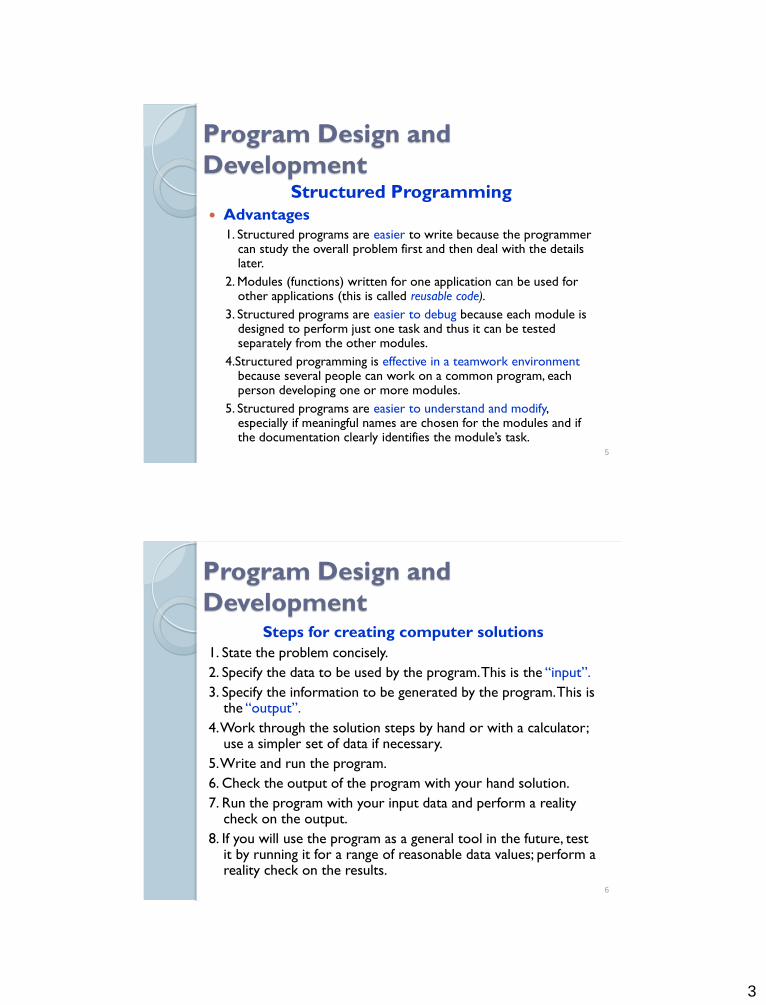
Advantages
1. Structured programs are easier to write because the programmer can study the overall problem first and then deal with the details later.
2. Modules (functions) written for one application can be used for other applications (this is called reusable code).
3. Structured programs are easier to debug because each module is designed to perform just one task and thus it can be tested separately from the other modules.
4.Structured programming is effective in a teamwork environment because several people can work on a common program, each person developing one or more modules.
5. Structured programs are easier to understand and modify, especially if meaningful names are chosen for the modules and if the documentation clearly identifies the module’s task.
5
Program Design and
Development Steps for creating computer solutions
1. State the problem concisely.
2. Specify the data to be used by the program. This is the “input”.
3. Specify the information to be generated by the program. This is the “output”.
4. Work through the solution steps by hand or with a calculator; use a simpler set of data if necessary.
5. Write and run the program.
6. Check the output of the program with your hand solution.
7. Run the program with your input data and perform a reality check on the output.
8. If you will use the program as a general tool in the future, test it by running it for a range of reasonable data values; perform a reality check on the results.
6

4
Program Design and
Development
Documentation
1. Proper selection of variable names to reflect the quantities
they represent.
2. Use of comments within the program.
3. Use of structure charts.
4. Use of flowcharts.
5. A verbal description of the program, often in pseudocode.
7
Program Design and
Development
Documenting with Charts
Two types of charts aid in developing structured programs
and in documenting them. These are structure charts and
flowcharts.
A structure chart is a graphical description showing how the
different parts of the program are connected together.
8

5
Program Design and
Development
Documenting with
Charts
Flowcharts are useful for
developing and documenting
programs that contain
conditional statements, because
they can display the various
paths (called “branches”) that a
program can take, depending on
how the conditional statements
are executed.
9
Program Design and
Development
Documenting with Pseudocode
We can document with pseudocode, in which
natural language and mathematical expressions are
used to construct statements that look like
computer statements but without detailed syntax.
Each pseudocode instruction may be numbered, but
should be unambiguous and computable.
10

6
Relational Operators
Six operators that are used for comparison of
variables (scalars or arrays) or expressions
They have equal precedence (evaluated from left to
right)
11
Relational Operators
For example, suppose that x = [6,3,9] and y = [14,2,9].
The following Matlab session shows some examples.
>>z = (x < y)
z = 1 0 0
>>z = (x ~= y)
z = 1 1 0
>>z = (x > 8)
z = 0 0 1
12
Note
Comparison is performed
element-wise

7
Relational Operators
The relational operators can be used for array addressing.
For example, with x = [6,3,9] and y = [14,2,9], typing
z = x(x<y)
finds all the elements in x that are less than the
corresponding elements in y. The result is z = 6.
The arithmetic operators +, -, *, /, and \ have precedence
over the relational operators. Thus the statement z = 5 > 2
+ 7 is equivalent to z = 5 >(2+7) and returns the result z =
0.
We can use parentheses to change the order of
precedence; for example, z = (5 > 2) + 7evaluates to z = 8.
13
The Logical Class
When the relational operators are used, such as x
= (5 > 2) they create a logical variable, in this case, x.
Prior to Matlab 6.5 logical was an attribute of any
numeric data type. Now logical is a first-class data
type and a Matlab class, and so logical is now
equivalent to other first-class types such as character
and cell arrays.
Logical variables may have only the values 1 (true)
and 0 (false).
14

8
Logical Operators
15
Logical Operators
16

9
Precedence of Different
Operators
17
Logical Functions
18

10
Logical Functions
19
Logical Functions
Use Matlab documentation to check the
following logical functions.
1. isstr
2. isnumeric
3. isvector
4. ishold
5. isequal
6. isscalar
20

11
The Find Function
The Matlab function find computes an array containing the indices of the nonzero elements of the numeric array x.
Example
>> x = [-2, 0, 4];
>> y = find(x)
Y = 1 3
The resulting array y = [1, 3] indicates that the first and third elements of x are nonzero.
[u,v,w] = find(A)
Computes the arrays u and v containing the row and column indices of the nonzero elements of the array A and computes the array w containing the values of the nonzero elements. The array w may be omitted.
21
The find Function
When the find function is used with arrays, the return value is the linear indices of the nonzero elements.
With linear indices, we can refer to array elements with a single value A(k), where k is the element location if the columns of the array are appended to each other.
Example A =
A(2) is equivalent to A(2,1) which is 5
A(5) is equivalent to A(2,2) which is 6
22
2 1 05 6 71 2 3

12
The Find Function
With logical operators
The expression inside the function is evaluated first, then the search for nonzero elements is performed
Consider the session >> x = [5, -3, 0, 0, 8]; y = [2, 4, 0, 5, 7];
>> z = find(x&y)
z = 1 2 5
Note that the find function returns the indices, and not the values.
To extract the values, use array indexing y = x(z)
23
Conditional Statements
The if statement’s basic form is
if logical expression
statements
end
Every if statement must have an accompanying end statement.
The end statement marks the end of the statements that are to be executed if the logical expression is true.
24

13
Conditional Statements
The else statement
The basic structure for the use of the else
statement is
if logical expression
statements group 1
else
statement group 2
end
25
Conditional Statements
26

14
Conditional Statements
Example
x = [4,-9,25];
if x < 0
disp(’Some elements of x are negative.’)
else
y = sqrt(x)
end
Because the test if x < 0 is false, when this program
is run it gives the result
y = [2, +3.000i, 5]
27
Conditional Statements
Example
x = [4,-9,25];
if x >= 0
y = sqrt(x)
else
disp(’Someelements of x are negative.’)
end
When executed, it produces the following message: Some elements of x are negative. The test if x < 0 is false, and the test if x >= 0 also returns a false value because x >= 0 returns the vector [1,0,1].
28

15
Conditional Statements
The elseif Statement
The general form of the if statement is if logical expression 1 statement group 1 elseif logical expression 2 statement group 2 else statement group 3 end
The else and elseif statements may be omitted if not required. However, if both are used, the else statement must come after the elseif statement to take care of all conditions that might be unaccounted for.
29
Conditional Statements
30

16
Conditional Statements
Example, suppose that
The following statements will compute y if x already has a scalar value
if x > 10
y = log(x)
elseif x >= 0
y = sqrt(x)
else
y = exp(x) -1
end
31
exp(x) 1,x 0
y sqrt(x),0 x 10
log(x),x 10
Loops
For Loops.
Used to repeat a set of statements for specific number of times.
The loop variable k is initially assigned the value 5, and x is calculated from x = k^2. Each successive pass through the loop increments k by 10 and calculates x until k exceeds 35. Thus k takes on the values 5, 15, 25, and 35, and x takes on the values 25, 225, 625, and 1225. The program then continues to execute any statements following the end statement.
32

17
33
Note the following rules when using for loops
with the
loop variable expression k = m:s:n
The step value s may be negative.
Example: k = 10:-2:4 produces k = 10, 8, 6, 4.
• If s is omitted, the step value defaults to 1.
• If s is positive, the loop will not be executed if m is greater than n.
• If s is negative, the loop will not be executed if m is less than n.
• If m equals n, the loop will be executed only once.
• If the step value s is not an integer, round-off errors can cause the loop to execute a different number of passes than intended.
34

18
Loops – The While Statement
The while loop is used when the looping process terminates because a specified condition is satisfied, and thus the number of passes is not known in advance.
The structure of a while loop
while logical expression
statements
end
For the while loop to function properly, the following two conditions must occur:
1.The loop variable must have a value before the while statement is executed.
2. The loop variable must be changed somehow by the statements.
35
Loops
While loop
A simple example of a while loop is
x = 5;
while x < 25
disp(x)
x = 2*x -1;
end
The results displayed by the disp statement are 5, 9, and 17.
36

19
Loops
Infinite Loops
You can create an infinite while loop which is a loop that never ends:
x = 8;
while x ~=0
x = x -3;
end
Within the loop the variable x takes on the values 5, 2, -1, -4….., and the condition x~=0 is always satisfied, so the loop never stops.
37
Loop Vectorization
We can often avoid the use of loops and branching and thus create simpler and faster programs by using a logical array as a mask that selects elements of another array. This called loop vectorization.
Example Here is one way to compute the sine of 1001 values ranging from 0 to 10:
i = 0;
for t = 0:.01:10
i = i + 1;
y(i) = sin(t);
End
A vectorized version of the same code is t = 0:.01:10 ;
y = sin(t) ; The second example executes much faster than the first and is the way Matlab is meant to be use
38

20
Loop Vectorization
Example: for the array A = [0, -1, 4; 9, -14, 25; -34, 49, 64], find all the elements that are greater than or equal to 0.
Using loops [m,n] = size(A) ;
C = zeros(m,n) ;
for k = 1:m*n
if A(k) >= 0
C(k) = A(k)
end
end
Using array masking and relational operators to vectorize
the loop C = A ;
C(C<0) = 0 ;
39
The Switch Structure
The switch structure provides an alternative to
using the if, elseif, and else commands. Anything
programmed using switch can also be
programmed using if structures. However, for
some applications the switch structure is more
readable than code using the if structure.
40

21
The Switch Statement
switch input expression
case value1
statement group 1
case value2
statement group 2
.
.
.
otherwise
statement group n
end 41
The Switch Statement
Example
The following switch block displays the point on the compass that corresponds to that angle.
switch angle case 45
disp(’Northeast’)
case 135
disp(’Southeast’)
case 225
disp(’Southwest’)
case 315
disp(’Northwest’)
otherwise
disp(’DirectionUnknown’)
end
42

22
Program Design and
Development
Finding Bugs
Debugging a program is the process of finding and removing the “bugs,” or errors, in a program. Such errors usually fall into one of the following categories.
1.Syntax errors such as omitting a parenthesis or comma, or spelling a command name incorrectly. Matlab usually detects the more obvious errors and displays a message describing the error and its location.
2. Runtime errors; These errors occur due to an incorrect mathematical procedure. They do not necessarily occur every time the program is executed; their occurrence often depends on the particular input data. A common example is division by zero.
43
Program Design and
Development
Locate Errors
1. Always test your program with a simple version of the problem, whose answers can be checked by hand calculations.
2. Display any intermediate calculations by removing semicolons at the end of statements.
3. To test user-defined functions, try commenting out the function line and running the file as a script.
4. Use the debugging features of the Editor/Debugger.
44

23
Matlab Editor/Debugger
Menus: File, Edit, text, Tools, Debug, Desktop, Window, Help
45
The Debug Menu
Breakpoints
Set/Clear Breakpoint
Step
Step In
Step Out
Continue
Go Until Cursor
Exit Debug Mode
Enable/Disable Breakpoint
Stop if Errors/Warnings
46

24
The Debug Menu
Example Two functions that find the values of a vector x that are
greater than the average values of all elements in x
47
% fun1.m function = fun1(x)
avg = sum(x) / length(x);
y= fun2(avg,x)
%fun2.m function fun2(x,avg)
above = length(find(x>avg));
>> % Test the functions
>> x = [1,2,3,4,10];
>> y = fun1(x)
y =
3
ERROR !!! Answer should be 1 !!!
Let’s see how we can debug …..
Strings
A string is a variable that contains characters.
Strings are useful for creating input prompts and messages and for storing and operating on data such as names and addresses.
To create a string variable, enclose the characters in single quotes.
For example, the string variable name is created as follows:
>>name = ’Leslie Student’
name =
Leslie Student
48

25
Strings and the Input Command
The input function, whose syntax is
x = input(’prompt’, ’s’)
displays the string prompt on the screen, waits for input
from the keyboard, and returns the entered value in the
string variable x.
49
Concatenating Strings
Given strings S1, S2, and S3, a string S that
is composed of appending the three stings
can be formulated by S = [S1 S2 S3]
concatenates character
Example >> S1 = ‘CPE’ ;
>> S2 = ‘0907311’;
>> S = [S1 S2]
S =
CPE0907311
50

26
Strings Conversion
Use the num2str() function to convert numeric values in strings.
Use the str2num() function to convert numeric values that are stored as strings to numbers.
Example
>> d = 1.23;
>> class(d)
ans = double
>> f = num2str(d)
f = 1.23
>> class(f)
ans = char
51

1
Computer Applications Lab
Lab 6
Plotting
Chapter 5
Sections 1,2,3,8
Dr. Iyad Jafar
Adapted from the publisher slides
Outline
xy Plotting Functions
Subplots
Special Plot Types
Three-Dimensional Plotting
2

2
xy Plotting The most common types of plots.
Plots the function y = f(x). (other symbols can be used also)
Anatomy of a plot
3
xy Plotting
The command that is used for xy plots in MATLAB is
plot(x,y)
where both x and y are vectors of the same length.
Example
The following MATLAB session plots y = 0.4 √1.8x for 0 ≤x ≤52, where y
represents the height of a rocket after launch, in miles, and x is the horizontal
(downrange) distance in miles.
>>x = [0:0.1:52];
>>y = 0.4*sqrt(1.8*x);
>>plot(x,y)
>>xlable(’Distance(miles)’) % Adds label to x-axis
>>ylable(’Height(miles)’) % Adds label to y-axis
>>title(’Rocket Height as a Function of Downrange Distance’)
% Adds title to the plot.
4

3
xy Plotting
5
xy Plotting
Requirements for a Correct Plot
1. Each axis must be labeled with the name of the quantity
being plotted and its units!
2. Each axis should have regularly spaced tick marks at
convenient intervals—not too sparse, but not too dense—
with a spacing that is easy to interpret and interpolate. For
example, use 0.1, 0.2, and so on, rather than 0.13, 0.26, and so
on.
3. If you are plotting more than one curve or data set, label
each on its plot or use a legend to distinguish them.
4. If you are preparing multiple plots of a similar type or if the
axes‟ labels cannot convey enough information, use a title.
6

4
xy Plotting Requirements for a Correct Plot
5 . If you are plotting measured data, plot each data point with a
symbol such as a circle, square, or cross (use the same symbol
for every point in the same data set). If there are many data
points, plot them using the dot symbol.
6. Sometimes data symbols are connected by lines to help the
viewer visualize the data, especially if there are few data
points. However, connecting the data points, especially with a
solid line, might be interpreted to imply knowledge of what
occurs between the data points. Thus you should be careful to
prevent such misinterpretation.
7. If you are plotting points generated by evaluating a function
(as opposed to measured data), do not use a symbol to plot the
points. Instead, be sure to generate many points, and connect the
points with solid lines.
7
xy Plotting The Figure Window
It has different menus to save, export, and edit
generated figures.
For example, we can
◦ save the figure to be used later on (it has .fig extension).
◦ print the plot
◦ we can insert text boxes, arrows, shapes, and legends.
◦ zoom in and out and rotate plot
◦ clear the figure
◦ copy the plot to be inserted in other documents
◦ export the figure in other data formats using File>Export
Setup
8

5
xy Plotting
More Commands grid command
The grid command displays gridlines at the tick marks corresponding to the tick labels.
Type grid on to add gridlines; type grid off to stop plotting gridlines. When used by
itself, grid toggles this feature on or off, but you might want to use grid on and grid off
to be sure.
axis command
Is used to override the MATLAB selections for the axis limits. The basic syntax is
axis([xmin xmax ymin ymax]). This command sets the scaling for the x-and y-axes
to the minimum and maximum values indicated. Note that, unlike an array, this command
does not use commas to separate the values.
figure command
Use this command to open a new figure window to be used for new plots. Using the plot
command more than once update the same figure window that was used by the first plot
command, unless the hold command is used
9
xy Plotting
10

6
xy Plotting Some Variations of the plot Command
If y is a vector and we use plot(y), MATLAB plots the
elements of y versus their indices.
If y is a vector of complex numbers, the use of plot(y) plots
the imaginary part of the elements versus the real part.
In other words, plot(y) in case y contains complex values is
equivalent to plot(real(y),imag(x)).
Example
>> z = 0.1 + 0.9i;
>> n = [0:0.01:10];
>> plot(z.^n),
xlabel(‘Real’),ylabel(‘imaginary’);
11
xy Plotting
The plot command with complex numbers
12

7
xy Plotting The function plot command fplot
It is a smart command that takes the function to be plotted
and determine the required number of points to show most
of the features of the function
Syntax
fplot(‘string’,[xmin xmax ymin ymax])
[x,y] = fplot(‘string’,[xmin xmax ymin ymax])
Example
compare the result of using fplot(‘cos(tan(x)) –
tan(sin(x))’,[1 2]) with
>> x = [1:0.01:2] ;
>> y = cos(tan(x)) – tan(sin(x));
>> plot(x,y)
13
xy Plotting
Using fplot command
14

8
xy Plotting
15
Using plot command
xy Plotting
Plotting Polynomials
The polyval(coeff,x) function in MATLAB can be used to
evaluate a polynomial whose coefficients are given in coeff
evaluated at values specified by x
Example
>> x = [-6:0.01:6];
>> y = [3,2,-100,2,-7,90];
>> plot(x,polyval(y,x))
>> xlable(‘x)
>> ylable(‘p’)
16
-6 -4 -2 0 2 4 6-3000
-2000
-1000
0
1000
2000
3000
4000
5000
p
x

9
xy Plotting
Subplots
You can use the subplot command to obtain several smaller “subplots”
in the same figure.
Syntax
subplot(m,n,p)
This command divides the Figure window into an array of rectangular
panes with m rows and n columns.
The variable p tells MATLAB to place the output of the plot
command following the subplot command into the pth pane.
For example, subplot(3,2,5)creates an array of six panes, three panes
deep and two panes across, and directs the next plot to appear in the
fifth pane (in the bottom-left corner).
17
xy Plotting
Subplots
Example
x = [0:0.01:5];
y = exp(-1.2*x).*sin(10*x+5);
subplot(1,2,1)
plot(x,y),axis([0 5 -1 1])
x = [-6:0.01:6];
y = abs(x.^3-100);
subplot(1,2,2)
plot(x,y),axis([-6 6 0 350])
18

10
xy Plotting - Example
19
xy Plotting Data Markers and Line Types
We can change the data markers, line styles, and colors for our plots by using a string in a
plot command
For example, plot(x,y,‟b-.o‟) plots y versus x using a blue dash-dotted line with circles as data
markers.
More data markers, line styles, and colors are listed below
20

11
xy Plotting
Controlling Tick-Mark Spacing and Labels
The set command is a powerful command for controlling objects
One of these objects is the axes in the plot.
We can change the tick mark spacing and use labels instead of numbers
as tick marks.
Syntax
Set(gca,’XTick’,[xmin:dx:xmax],’YTick’,[ymin:dy:ymax])
◦ gca is a function that returns a handle for the current axes
Example
set(gca,’XTick’,[0:0.1:2],’YTick’,[0:0,1:1])
21
xy Plotting
Controlling Tick-Mark Spacing and Labels
We can assign labels to tick marks instead of numbers.
Example >> x = [1:6];
>> y = [13,5,7,14,10,12]
>> set(gca,‟Xticklabel‟,[„Jan‟;‟Feb‟;‟Mar‟;Apr‟;‟May‟;‟Jun‟])
>> set(gca,‟XTick„,[1:6]), axis([1 6 0 15]) , xlabel(„Month‟) …
,ylabel(„Monthly Sales $1000‟), title(„Printer Sales for January to June, 1997‟)
22

12
xy Plotting
Labeling Curves and Data When we plot more than one curve on the same plot, we
have to distinguish them with ◦ Legends
legend(‘string1’,’string2’,…)
◦ By a label next to each curve
gtext(‘string’) (it requires user interaction to specify the location of the text by the mouse)
or use
text(x,y,’string’) where x and y specify the location of the text
Example
23
xy Plotting
24

13
xy Plotting
The hold Command
We can plot y versus x and v versus u on the same figure using the plot
command by
plot(x,y,u,v)
If we use the plot command once more, the figure gets updated with the
new plot and the old plot is erased.
To preserve earlier plots, use the hold on command.
This command will allow the new plot to be superimposed over the old
plot.
Use hold off to disable the hold command.
25
xy Plotting
Annotating Plots
We already saw the title(‘string’) that is used to insert a title for the plot.
We can insert mathematical symbols in the title, axes labels, and text
labels by using the backslash character \ followed by the symbol name.
Superscripts and subscripts are denoted by ^ and _ , respectively. To set
multiple characters as superscripts or subscripts, enclose them by {}.
Example : the command
>> title(‘Ae^{-t/\tau} sin(\omega t)’)
produces
in the figure title.
26
t/Ae sin( t)

14
xy Plotting Hints for Improving Plots
1. Start scales from zero whenever possible. This technique prevents a false
impression of the magnitudes of any variations shown on the plot.
2. Use sensible tick-mark spacing. If the quantities are months, choose a
spacing of 12 because 1/10 of a year is not a convenient division. Space
tick marks as close as is useful, but no closer. If the data is given monthly
over a range of 24 months, 48 tick marks might be too dense, and also
unnecessary.
3. Minimize the number of zeros in the data being plotted. For example, use
a scale in millions of dollars when appropriate, instead of a scale in dollars
with six zeros after every number
4. Determine the minimum and maximum data values for each axis before
plotting the data. Then set the axis limits to cover the entire data range
plus an additional amount to allow convenient tick-mark spacing to be
selected.
27
xy Plotting Hints for Improving Plots
5. Use a different line type for each curve when several are plotted on a
single plot and they cross each other; for example, use a solid line, a
dashed line, and combinations of lines and symbols. Beware of using
colors to distinguish plots if you are going to make black-and-white
printouts and photocopies.
6. Do not put many curves on one plot, particularly if they will be close to
each other or cross one another at several points.
7. Use the same scale limits and tick spacing on each plot if you need to
compare information on more than one plot
28

15
xy Plotting Special Types of Plots
Exercise: use the help browser to check the stairs
command.
29
0 1 2 3 4 5 6 7 8 9 100
1
2
3
4
5
6
7
8
9
10
x
y
Stem Plots: use stem(x,y) Bar Plots: use bar(x,y)
1 4 5 8 90
1
2
3
4
5
6
7
8
9
10
x
y
3-D Plotting Plotting of Curves
Use the command plot3(x,y,z) to plot three-
dimensional curves.
We can use the grid command and the attributes for
selecting the line style, color and data markers.
Example
30

16
3-D Plotting
Surface Mesh Plots
The function z = f(x,y) represents a surface
when plotted on xyz axes, and the mesh
function provides the means to generate a
surface plot. Before you can use this function,
you must generate a grid of points on the xy-
plane, and then evaluate the function f(x,y) at
these points. The meshgrid function
generates the grid.
31
3-D Plotting
Surface Mesh Plots
Syntax
[X,Y] = meshgrid(x,y)
Where x = [xmin:xspacing:xmax] and y = [ymin:yspacing:ymax],
This computes the Cartesian product between x and y.
The function [X,Y] = meshgrid(x) is the equivalent to [X,Y] =
meshgrid(x,x) and can be used if x and y have the same minimum
values, the same maximum values, and the same spacing. Using this
form, you can type [X,Y] = meshgrid(min:spacing:max), where min and
max specify the minimum and maximum values of both x and y and
spacing is the desired spacing of the x and y values.
Once the grid is obtained, we can plot the three dimensional surface
using the mesh(x,y,z) function. As always, the grid, label, and text
functions can be used with the mesh function.
32

17
3-D Plotting
Surface Mesh Plots
Example
33
3-D Plotting Contour Plots
Contour plot contain lines that indicate constant elevation (values).
Contour plots can be generated in MATLAB by the contour(x,y,z) command.
We need first to use the meshgrid.
34

18
3-D Plotting
35
3-D Plotting Examples
36
mesh(x,y,z) meshc(x,y,z)
meshz(x,y,z) waterfall(x,y,z)

1
Computer Applications Lab
Lab 7
Designing GUI with Matlab
Dr. Iyad Jafar
Adapted from Mathworks
Outline
What is Graphical User Interface (GUI) ?
GUI in Matlab
How does GUI work ?
Structure of GUI in Matlab
The GUIDE Tool
Structure of GUI M-File
A Simple GUI Example
Adding Menus
2

2
What is GUI ? A graphical user interface (GUI) is a graphical display that
contains devices, or components, that enable a user to
perform interactive tasks.
To perform these tasks, the user of the GUI does not have
to create a script or type commands at the command line.
Often, the user does not have to know the details of the
task at hand.
3
How Does a GUI Work?
Each component, and the GUI itself, is associated with one or more user-written routines known as callbacks. The execution of each callback is triggered by a particular user action such as a button push, mouse click, selection of a menu item, or the cursor passing over a component. You, as the creator of the GUI, provide these callbacks.
This kind of programming is often referred to as event-driven programming.
The writer of a callback has no control over the sequence of events that leads to its execution or, when the callback does execute.
4

3
Structure of GUI in Matlab
Any GUI in MATALB is associated with two files
◦ Figure file with extension .fig that contains all the components or controls to be used in the GUI application. The FIG-file is a binary file and you cannot modify it except by changing the layout in GUIDE.
◦ M-file that contains the code for the GUI initialization and the callbacks/functions for different components in the GUI layout and other hidden functions of the GUI.
5
Creating GUI Using GUIDE
GUIs in Matlab can be created either
programmatically or by using the GUIDE
tool.
Type guide on the command prompt to
start the GUIDE tool.
With this tool, you can use the mouse to
add different components and set their
properties (size, text, callbacks)
6

4
7
8
Use This Tool... To...
Layout Editor Select components from the component palette, at the left side of the Layout
Editor, and arrange them in the layout area. See Adding Components to the GUI for
more information.
Figure Resize Tab Set the size at which the GUI is initially displayed when you run it. See Setting the
GUI Size for more information.
Menu Editor Create menus and context, i.e., pop-up, menus. See Creating Menus for more
information.
Align Objects Align and distribute groups of components. Grids and rulers also enable you to
align components on a grid with an optional snap-to-grid capability. See Aligning
Components for more information.
Tab Order Editor Set the tab and stacking order of the components in your layout. See Setting Tab
Order for more information.
Toolbar Editor Create Toolbars containing predefined and custom push buttons and toggle buttons.
See Creating Toolbars for more information.
Icon Editor Create and modify icons for tools in a toolbar. See Creating Toolbars for more
information.
Property Inspector Set the properties of the components in your layout. It provides a list of all the
properties you can set and displays their current values.
Object Browser Display a hierarchical list of the objects in the GUI. See Viewing the Object
Hierarchy for more information.
Run Save and run the current GUI. See Saving and Running a GUIDE GUI for more
information.
M-File Editor Display, in your default editor, the M-file associated with the GUI. See GUI Files: An
Overview for more information.
Position Readouts Continuously display the mouse cursor position and the positions of selected
objects

5
Structure of GUI M-file
The GUI M-file that GUIDE generates is a function file. It has the same name as the GUI figure file.
It contains the callbacks for the GUI components which are subfunctions of the main function.
When GUIDE generates an M-file, it automatically includes templates for the most commonly used callbacks for each component.
The M-file also contains initialization code, as well as an opening function callback and an output function callback.
You must add code to the component callbacks for your GUI to work as you want.
9
Structure of GUI M-file Example, the GUI opening function % --- Executes just before simple_gui is made visible.
function simple_gui_OpeningFcn(hObject, eventdata, handles, varargin)
% This function has no output args, see OutputFcn.
% hObject handle to figure
% eventdata reserved - to be defined in a future version of Matlab
% handles structure with handles and user data (see GUIDATA)
% varargin command line arguments to simple_gui (see VARARGIN)
% Choose default command line output for simple_gui
handles.output = hObject;
handles.x = 7
% Update handles structure
guidata(hObject, handles);
The handles argument is an important structure that contains the data of the GUI. This structure is available for all components in the GUI. It can be used to store any data.
10

6
Structure of GUI M-file
Example, callback function for a pushbutton % --- Executes on button press in pushbutton1.
function pushbutton1_Callback(hObject, eventdata, handles)
% hObject handle to pushbutton1 (see GCBO)
% eventdata reserved - to be defined in a future version
of Matlab
% handles structure with handles and user data (see
GUIDATA)
handles.x = sqrt(5)
% Update handles structure
guidata(hObject, handles);
Each time the handles data is modified, the function guidata has to be used to save the new data to the handles structure.
11
The Get function
The get function is extensively used in programming GUIs. It is used to get properties and values of the GUI component.
Syntax
get(h,'PropertyName')
h is a handle to the component and propertyName is the name of the property that we want to get for the component specified by the handle.
Components handles can specified using the handles.tagValue, where tagValues is the vaule of the tag property for the component.
12

7
The Set Function
The set function is the opposite of the get
function.
It is used to change the value of certain
property of a component.
Syntax set(h,'PropertyName',PropertyValue,...)
The properties differ from component to
component.
13
Components Properties
Each GUI component has its own properties that can be changed by the property inspector or by the set function.
Some of these properties are
◦ ‘String’, ‘fontWeight’, ‘fontSize’, ‘fontName’, ‘fontAngle’, which are used to format and specify the component label.
◦ ‘value’ property depends on component type.
◦ ‘Tag’ is the name of the component that is used to get and set its properties in the code.
◦ ‘Enable’ is used to disable or enable the component.
◦ ‘Visible’ controls if the component is visible or not.
◦ ‘Resize’ enable or disable resizing fo components or the GUI figure.
14
8
Example
We want to create a GUI that plots a sine or a cosine function over a range that is specified by the user. When the GUI is started, the default plot is a sine wave over [-π,π] with 100 points. The user should have the option to show or hide gridline
Required components ◦ Axes to plot the function.
◦ Popmenu to allow the user to choose which function to plot.
◦ Two text boxes to specify the minimum and the maximum of the range.
◦ One text box to specify the number of points to be used in the plot
◦ A push button to update the plot based on the user input.
◦ A check box to show or hide gridlines
15
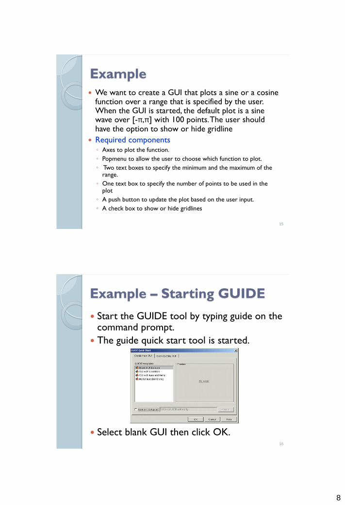
Example – Starting GUIDE
Start the GUIDE tool by typing guide on the command prompt.
The guide quick start tool is started.
Select blank GUI then click OK.
16

9
Example – Adding Components
Use the GUI preferences from the File menu to display the names of the components.
17
Example – Adding Components Using the mouse, drag and drop the required
components in the figure
18

10
Example – Adding Components Use the property editor to change the labels of different
components. Change the property ‘String’ for each component.
19
Example - Saving
Save your GUI with the name guiExample by clicking on save from the File menu.
Matlab will create two files
◦ guiExample.fig
◦ guiExample.m
Matlab will open the editor to show the contents of the guiExample.m file.
The m-file contains the common callbacks for different components in the GUI.
20

11
Example - Programming the GUI
Initialization part
We want the GUI to generate a default plot
when it is first started. This code is added to
the opening function of the GUI.
In the M-file editor, click on show function
icon . . A menu will appear listing all
functions in the M-file.
Select guiExample_OpeningFcn. The editor
goes to the line where this function starts.
Add the following code to opening function.
21
Example - Programming the GUI % Set the values for the text boxes to default values
% access the handles for the text boxes from the handles
structure
set(handles.xMin,'string',num2str(-pi))
set(handles.xMax,'string',num2str(pi))
set(handles.nPoints,'string',num2str(100))
% define default range, points, and function to be
plotted
xMin = -pi , xMax = pi , nPoints = 100 ;
% define default range, points, and function to be plotted
x = xMin: (xMax-xMin)/(100-1):xMax;
y = sin(x) ;
plot(x,y), xlabel(‘x’),ylabel(‘y’);
% Update handles structure
guidata(hObject, handles);
22

12
Example - Programming the
GUI
Programming the Push Button
The callback function of the push button should perform the following tasks:
◦ Read the minimum and maximum of the plotting range from xMin and xMax textboxes.
◦ Read the number of points to be used from nPoints textbox.
◦ Read the function to be plotted from the popmenu.
◦ Plot the required function based no user selection.
Select the plotButton callback function from the function icon . . Insert the following code in the function.
23
Example - Programming the
GUI
Programming the Push Button % when this key is pressed, we have to read the values from the text
boxes
% and the function to be plotted, the plot.
xMin = str2num(get(handles.xMin,'string'));
xMax = str2num(get(handles.xMax,'string'));
nPoints = str2num(get(handles.nPoints,'string'));
func = get(handles.funcMenu,'value')
% generate x vector and plot the function based on the value of the popmenu
x = xMin : (xMax-xMin)/(nPoints-1) : xMax ;
if func == 1
plot(x,sin(x));
title('Sin(x)'), xlabel('x'),ylabel('y');
else
plot(x,cos(x));
title('cos(x)'), xlabel('x'),ylabel('y');
end
%clear selection of the grid checkbox
set(handles.gridChkBox,'value',0)
24

13
Example - Programming the
GUI
Programming the Checkbox
When this checkbox is on, gridlines should appear on the axes of the GUI. When it is not selected, no gridlines are shown.
To program this, just add the grid command in the body of the checkBox callback function (the tag name is gridChkBox).
Each time the checkbox is selected or deselected, the function is executed and the use of the grid command toggles the gridlines.
25
Final GUI
26

14
Notes
To run your GUI, type its name on the command prompt. Or click on the run icon in GUIDE.
To open your GUI, start the guide tool then click on the open existing GUI tab and select your file.
To close your GUI from your code, use the close command.
If you have more than one axes in your GUI and you want activate one of them for plotting, use axes(h) where h is a handle to axes. Example axes(handles.axes1) set axes1 in the GUI as the current axes.
27
Adding Menus We can add menus to our GUI similar to those found in
most GUI application. Let’s add a File menu to the
previous example. The menu should contain two items:
close, to close the GUI, and reset to clear the axes and
the text boxes.
This can be done using the menu editor.
Click on the menu editor icon to start the menu
editor.
28

15
Adding Menus
Click on the new menu icon to insert a
new menu. Click on the new menu and
update its properties as shown.
29
Adding Menus
Click on the new menu item icon and add
two items with labels Reset and Close, and tags
restItem and closeItem.
30

16
Adding Menus
Now if you run you GUI by clicking on the
run icon in GUIDE, you will see the
created menu.
31
Adding Menus
We need now to define the callbacks for the menus items.
In the editor, select resetItem_callback from the funtion list and add the following line of code
% clear current axes1
cla(handles.axes1)
set(handles.xMin,'string','')
set(handles.xMax,'string','')
set(handles.nPoints,'string','')
set(handles.gridChkBox,'value',0)
Similarly, add the close command to the callback function of closeItem to close the GUI.
32

17
The uigetfile Command
The uigetfile command opens the standard box for retrieving files. It can be used with other data importing functions to open files interactively.
Syntax [FileName,PathName,FilterIndex] = uigetfile(FilterSpec)
The returned values are strings
Example:
>> [fName,fPath,fInex] = uigetfile(‘*.csv’) ;
>> % Matlab will open the dialog box
>> class(fName)
ans =
char
33
The uigetfile Command
If the Cancel button is pressed, an empty string is returned.
34

18
The msgbox Command
We can generate message windows by
using the msgbox command.
Syntax msgbox(Message,Title,Icon)
Message is the message to be displayed as
string.
Title is the title of the window as a string.
Icon is the icon to be displayed on the
message. It can be ’error’, ‘help’, or ‘warn’.
35
The msgbox Command
Example msgbox(‘Division by Zero’,’My
Message’,’Warn’)
36

1
Computer Applications Lab
Lab 9 Probability, Statistics, Interpolation,
and Calculus
Chapter 7
Dr. Iyad Jafar
Adapted from the publisher slides
Outline
Statistics and Probability
Histograms
Normal and Uniform Distributions
Random Number Generation
Interpolation
2

2
Common Statistical Functions MATALB provides several functions to compute statistical properties of
any set of numerical data
For the first three commands, if x is a matrix, Matlab returns a raw vector
in which each element is the result of applying these function to its
columns. cumsum returns a matrix that contains cumulative sums of the
columns.
3
Function Description
mean (x) Computes the average value for the elements of vector x.
median(x) Computes the median value for the elements in vector x.
std(x) Computes the standard deviation of the elements in vector
x.
cumsum(x) Returns a vector the same size of x containing the
cumulative sum of the elements in x.
Examples
>> x =[ones(1,5)*3,ones(1,4),ones(1,6)*(2)];
>> mean(x)
ans = 31
>> median(x)
ans = 2
>> std(x)
ans = 0.7988
>> cumsum(x)
ans = 3 6 9 12 15 16 17
18 19 21 23 25 27 29
31
4

3
Histograms Given a set of data values stored in vector x, the histogram of x
is a display of statistical information that uses rectangles to
show the frequency of data items in successive numerical
intervals of equal size.
Histograms are useful in studying data properties and
distribution as they can be used to approximate the probability
function.
Suppose x = [1,1,1,3,4,4,5,5,5,6,6,7,7,7,7,7,7], the histogram of
these values is shown below.
5 0 1 2 3 4 5 6 7 80
1
2
3
4
5
6
7Histogram of x
x
Absolu
te F
requency
Histograms
To generate histograms in MATALB, use the ◦ hist(x) function or its variants (discussed later)
◦ bar(x,y), where x is a vector containing the centers of the bars (counts) and y is a vector containing the frequencies of the values in each bar.
Example
>> x = [1,1,1,3,4,4,5,5,5,6,6,7,7,7,7,7,7];
>> hist(x,[0:8]); % here we specified the bin centers. If not provided, Matlab default is 10 bins between the min and max of input data
OR
>> x = [0:8] ; % specify bar centers
>> y = [0,3,0,1,2,3,2,6,0]; % absolute frequencies manually computed
>> bar(x,y);
6

4
Histograms
7
Command Description
bar(x,y) Creates a bar chart of y versus x.
hist(y) Aggregates the data in the vector y into 10 bins evenly spaced
between the minimum and maximum values in y.
hist(y,n) Aggregates the data in the vector y into n bins evenly spaced
between the minimum and maximum values in y.
hist(y,x) Aggregates the data in the vector y into bins whose center
locations are specified by the vector x. The bin widths are the
distances between the centers.
[z,x] = hist(y) Same as hist(y) but returns two vectors z and x that contain
the frequency count and the bin locations.
[z,x] = hist(y,n) Same as hist(y,n) but returns two vectors z and x that contain
the frequency count and the bin locations.
[z,x] = hist(y,x) Same as hist(y,x) but returns two vectors z and x that contain
the frequency count and the bin locations. The returned vector
x is the same as the user-supplied vector x
Probability In any experiment or phenomena, the probability of
an event is a number between 0 and 1 that indicates the likelihood of that event to occur if the experiment is repeated infinitely
Example: Rolling a dice. The probability of obtaining any of the number on the dice is 1/6.
Random variable is often the term used to express the outcome of an experiment. In rolling a dice, the random variable may take any of the values 1,2,3,4,5,6.
Based on the experiment, these random variables could be continuous or discrete.
8

5
Probability - Example
9
Probability – Probability Functions
Random variables are usually associated with
functions or distributions to characterize the
experiment they come from.
Such functions are called probability density functions
(pdf).
If available, these distributions can be used to
calculate the probability of the random variable to
take certain value(s).
The area under pdf is always equal to 1. this is based
on the fact that we will obtain any of the possible
outcomes if we run the experiment.
10

6
Common Distributions
Uniform Distribution
Normal Distribution
11
1 , a x b
pdf(x) b a 0 , otherwise
2
2(x )
21pdf(x) e
2
ba
b - a
_____1
-6 -4 -2 0 2 4 60
0.05
0.1
0.15
0.2
0.25
0.3
0.35
0.4
0.45
Computing Probability of an Event
The probability that a random variable x is less than or equal than some value b is computed from the pdf by
Continuous RV Discrete RV
This is usually referred as the cumulative distribution function CDF.
For continuous random variables, the probability P(x=b) = 0.
For discrete random variables, the probability P(x=xk) = pdf(xk)
12
b
P(x b) pdf(x)dx CDF(x)
k
k ii
P(x x ) pdf(x)

7
Histograms as pdf
For practical experiments, it is common
to use the normalized histogram to
represent the pdf of the experiment.
The normalized histogram is defined as
the absolute frequency histogram divided
by total number of frequencies.
13
Example Suppose that x = [1,1,1,1,1,2,2,3,3,3,3,5,5,5,5,7,7,7,7,7,7,7,8]
The following commands generates the normalized histogram of x with
bin centers at 1 through 8.
>> [y,binLocations] = hist(x,[1:8]) ;
>> normhist = y / sum(y) ; % or could use normhist = y / length(x)
>> label(‘x’)
>> ylabel(‘Normalized Histogram’)
The probability of obtaining a number less than or equal to 3 can be found by
>> cdf = cumsum(normhist)
>> prob = cdf(3)
14 1 2 3 4 5 6 7 8
0
0.05
0.1
0.15
0.2
0.25
0.3
0.35
x
Nor
mal
ized
His
togr
am

8
Sums and Differences of
Random Variables
15
It can be proved that the mean of the sum (or difference)
of two independent normally distributed random variables
equals the sum (or difference) of their means, but the
variance is always the sum of the two variances. That is,
if x and y are normally distributed with means x and y,
and variances x and y, and if u x + y and u x y,
then
u x + y
u x y
u2 u
2 x2 + y
2
Random Numbers
Random numbers are extensively used in
simulation and game programming.
Matlab provides several functions to
generate random numbers based on a given
distribution.
16

9
Random Numbers
17
Command Description
rand Generates a single uniformly distributed random number
between 0 and 1.
rand(n) Generates an n x n matrix containing uniformly
distributed random numbers between 0 and 1.
rand(m,n) Generates an m x n matrix containing uniformly
distributed random numbers between 0 and 1.
s = rand(’state’) Returns a 35-element vector s containing the current
state of the uniformly distributed generator.
rand(’state’,s) Sets the state of the uniformly distributed generator to s.
rand(’state’,0) Resets the uniformly distributed generator to its initial
state.
rand(’state’,j) Resets the uniformly distributed generator to state j, for
integer j.
rand(’state’,sum(100*clock)) Resets the uniformly distributed generator to a different
state each time it is executed.
Random Numbers
18
Command Description
randn Generates a single normally distributed random number having
a mean of 0 and a standard deviation of 1.
randn(n) Generates an n ´ n matrix containing normally distributed
random numbers having a mean of 0 and a standard deviation of
1.
randn(m,n) Generates an m ´ n matrix containing normally distributed
random numbers having a mean of 0 and a standard deviation of
1.
s = randn(’state’) Like rand(’state’) but for the normally distributed generator
randn(’state’,s) Like rand(’state’,s) but for the normally distributed generator.
randn(’state’,0) Like rand(’state’,0) but for the normally distributed generator.
randn(’state’,j) Like rand(’state’,j) but for the normally distributed generator.
randn(’state’,sum(100*clo
ck))
Like rand(’state’,sum(100*clock)) but for the normally
distributed generator.

10
Random Numbers
Example: check the operation of randn >> x = randn(1,10000);
>> [y,bins] = hist(x,[-4:0.01:4]));
>> y = y / length(x)
>> Bar(bins,y)
>> axis([-5 5 0 max(y)*1.1])
19 -5 -4 -3 -2 -1 0 1 2 3 4 5
0
1
2
3
4
5
x 10-3
Random Numbers To generate uniformly distributed random
numbers in the interval [a,b], use
y = (b-a) * x + a
Where x is a set of uniformly distributed numbers generated by rand function.
Example : the following session generates 1000 uniformly distributed numbers in the interval [-3,3].
>> x = rand(1,1000) ;
>> y = (3+3) * x – 3 ;
>> [yhist,bins] = hist(y,[-4:0.1:4]);
>> bar(bins,yhist);
20

11
Random Numbers
-5 -4 -3 -2 -1 0 1 2 3 4 50
5
10
15
20
25
30
x
Appro
xim
ate
Uniform
Dis
trib
ution
21
Random Numbers
To generate normally distributed random numbers with a mean µ and standard deviation σ
y = σ * x + µ
Where x is a set of normally distributed numbers generated by randn function.
Example : the following session generates 1000 normally distributed numbers with a mean of 5 and deviation of 1.5
>> x = randn(1,1000) ;
>> y = 1.5* x + 5 ;
>> [yhist,bins] = hist(x,[0:0.1:10];
>> bar(bins,yhist);
22

12
Random Numbers
-2 0 2 4 6 8 10 120
5
10
15
20
25
30
35
x
Appro
xim
ate
Norm
al D
istr
ibution
23
Interpolation
Engineering problems often require the analysis of data pairs; cause and effect, or input output relationships.
It is sometimes required to estimate variable’s value between the given data point. This process is known as interpolation.
Plotting the data greatly aids interpolation and extrapolation.
24

13
Interpolation Linear and cubic spline interpolation
25
0 1 2 3 4 5 60
1
2
3
4
5
6
7
8
x
y
Linear
Cubic Spline
Interpolation
26
Function Description
Y_int =
interp1(x,y,x_int)
Used to linearly interpolate a function of one variable: y f (x). Returns a linearly interpolated vector y_int at the
specified value x_int, using data stored in x and y.
Z_int =
interp2(x,y,z,x_int,y
_int)
Used to linearly interpolate a function of two variables: y f (x, y). Returns a linearly interpolated vector z_int at
the specified values x_int and y_int, using data stored
in x, y, and z.
Y_int =
spline(x,y,x_int)
Computes a cubic-spline interpolation where x and y
are vectors containing the data and x_int is a vector
containing the values of the independent variable x at
which we wish to estimate the dependent variable y. The
result Y_int is a vector the same size as x_int containing
the interpolated values of y that correspond to x_int.

14
Interpolation
When using interp1 or spline functions, note that x should be sorted in ascending order and x_int values should be within the range of x.
Example: assume that x = [1,2,3,4,5] and y = [2,5,8,10,6]. Estimate the value of y when x_int = [2.5,3.5].
% using linear
>> y_int = interp1(x,y,x_int)
y_int = 6.5000 9.0000
% using cubic spline
>> y_int = spline(x,y,x_int)
y_int = 6.5000 9.3750
27

1
Computer Applications Lab
Lab 10 Numerical Calculus and Symbolic
Processing
Chapter 8 - Sections 8.1 through 8.3
Chapter 10 - Sections 10.1 through 10.3
Dr. Iyad Jafar
Adapted from the publisher slides
Outline
Numerical Calculus
◦ Integration
◦ differentiation
Symbolic Processing ◦ Defining symbolic expressions
◦ Manipulation of symbolic expressions
◦ Symbolic differentiation, integration, and limits
2

2
Numerical Calculus - Integration
Integration of function f(x) in the interval a ≤ x ≤
b can be represented as the area between f(x) and
the x-axis.
3
Numerical Calculus - Integration
Numerical integration can be approximated by
partitioning the area into rectangles or trapezoidals
then summing up their areas.
4

3
Numerical Calculus - Integration
5
Function Description
trapz(x,y) Uses trapezoidal integration to compute the integral
of y with respect to x, where the array y contains the
function values at the points contained in the array x.
quad(‘func’,a,b,tol) Uses an adaptive Simpson’s rule to compute the
integral of the function ’fun’ with a as the lower
integration limit and b as the upper limit. The
parameter tol is optional. tol indicates the specified
error tolerance.
quad1(‘fun’,a,b,tol) Uses Lobatto quadrature to compute the integral of
the function ’fun’. The rest of the syntax is identical to
quad.
Numerical Calculus - Integration
The quad and quadl functions are more accurate than trapz; however, they are restricted to computing the integrals of functions and cannot be used when the integrand is specified by a set of points. For such cases, use the trapz function.
Example: the integration can be computed in Matlab
6
Function Result
quad(‘sin’,0,pi) 2
quad1(‘sin’,0,pi) 2
x = 0:0.01:pi
trapz(x,sin(x)) 1.9797
0
sin(x)dx 2

4
Numerical Calculus - Differentiation
The derivative of a function can be interpreted
graphically as the slope function.
Three methods can be used to estimate the slope at
a point numerically; backward difference, forward
difference, and central difference.
7
Matlab provides the diff function for computing derivative estimates. It computes the backward difference.
Syntax
d = diff(x)
where x is a vector of values and the result is a vector d containing the differences between adjacent elements in x.
if x has n elements, then d is n-1 elements.
Example:
>> x = [5,7,12,-20];
>> y = diff(x)
y = 2 5 -32
8
Numerical Calculus - Differentiation

5
Example: compare the true derivative of sin(x) with backward and central derivatives.
x = [0:pi/50:2*pi] ;
n = length(x);
y = sin(x);
% true derivative
td = cos(x) ;
% numerical derivative backward difference
nd = diff(y) ./ diff(x) ;
% numerical derivative using central difference
ncd = (y(3:n)-y(1:n-2))./ (x(3:n)-x(1:n-2)) ;
plot(x,td,'b'), ;hold on
plot(x(2:n),nd,'ro'), plot(x(3:n),ncd,'g*') ;
xlabel('x'), ylabel('Derivative of SIN(x)')
legend('COS(x)','Backward Derivative','Central Derivative')
9
Numerical Calculus - Differentiation
10
0 1 2 3 4 5 6 7-1
-0.8
-0.6
-0.4
-0.2
0
0.2
0.4
0.6
0.8
1
x
Derivative o
f S
IN(x
)
COS(x)
Backward Derivative
Central Derivative
Numerical Calculus - Differentiation

6
11
Command Description
d = diff(x)
Returns a vector d containing the differences between adjacent
elements in the vector x.
b = polyder(p)
Returns a vector b containing the coefficients of the derivative
of the polynomial represented by the vector p.
b =
polyder(p1,p2)
Returns a vector b containing the coefficients of the polynomial
that is the derivative of the product of the polynomials represented by p1 and p2.
[num, den] =
polyder(p2,p1)
Returns the vectors num and den containing the coefficients of
the numerator and denominator polynomials of the derivative of the quotient p2/p1, where p1 and p2 are polynomials.
Numerical Calculus - Differentiation
Example
F(x) = x2 + 2x + 1 , G(x) = x3 + 5x2 – x + 8, find the derivative of F * G and F/G
>> F = [1,2,1], G = [1,5,-1,8];
% d/dx(F*G) >> d = polyder(F,G)
d = 5 28 30 22 15
% d/dx(F/G) >> [num,denum] = polyder(F,G)
num = -1 -4 -14 6 17
denum = 1 10 23 6 81 -16
64
12
Numerical Calculus - Differentiation

7
Symbolic Processing
Refers to the way that computers
perform operations on mathematical
expressions the way that humans it with
pencil and paper.
Matlab contains many functions to define
symbols, symbolic expressions,
simplification, and solution to symbolic
expressions.
13
Symbolic Processing – Defining Symbols
To define a symbol in Matlab use the sym() or the syms functions. We can create symbolic constants or symbolic variables.
Examples
1. x = sym(‘x’) % creates the symbolic variable with name x
2. syms x y u v % creates four symbolic variables x,y,u, and v
3. fraction = sym(‘1/3’) % create symbolic constant fraction with value 1/3
When mathematical operations are used with symbols, the result is symbolic.
Example >> x = sym(‘sqrt(2)’);
>> 2 * x
ans = 2*2^(1/2)
>> class(ans)
ans = sym
14

8
Symbolic Processing – Symbolic
Expressions We can use symbols to define symbolic expressions. We can use the
operators + - / ^ and the built-in functions.
Example
>> syms x y ;
>> r = sqrt(x^2+y^2)
r = (x^2+y^2)^(1/2)
If we later assign x and y to 3 and 5, typing r will not result in the evaluation
of the expression.
We can use the vector and matrix notation with symbols.
Example
>> n = 3 , syms x, A = x.^((0:n)’*(0:n))
A = [ 1, 1, 1, 1]
[ 1, x, x^2, x^3]
[ 1, x^2, x^4, x^6]
[ 1, x^3, x^6, x^9]
>> class(A)
ans = sym
15
Symbolic Processing The function findsym(E,n) returns the n symbolic variables in
expression E that are closest to x (default symbol in Matlab), with
the tie breaker going to the variable closer to z. >>syms b x1 y
>>findsym(6*b+y)
ans =
b,y
>>findsym(6*b+y,1) %Find the one variable closest to
x
ans =
y
>>findsym(6*b+y+x1,1) %Find the one variable closest
to x
ans =
x1
>>findsym(6*b+y*i) %i is not symbolic
ans =
b, y 16

9
Manipulating Symbolic Expressions
With symbolic expressions in Matlab, we can expand, collect, simplify, and
create new expressions from old expressions using the mathematical
operators.
The function collect(E) collects coefficients of like powers in the
expression E. If there is more than one variable, you can use the optional
form collect(E,v), which collects all the coefficients with the same
power of v.
>>syms x y
>>E = (x-5)^2+(y-3)^2;
>>collect(E) % will collect x powers
ans =
x^2-10*x+25+(y-3)^2
>>collect(E,y) % will collect y powers
ans =
y^2-6*y+(x-5)^2+9
17
Manipulating Symbolic Expressions
The expand and simplify functions. >>syms x y
>>expand((x+y)^2) % applies algebra rules
ans =
x^2+2*x*y+y^2
>>expand(sin(x+y)) % applies trig identities
ans =
sin(x)*cos(y)+cos(x)*sin(y)
>>simplify(6*((sin(x))^2+(cos(x))^2))
% applies another trig identity
ans = 6
18

10
Manipulating Symbolic Expressions
The factor function finds the factors of the expression.
>>syms x y
>>factor(x^2-1)
ans =
(x-1)*(x+1)
The function subs(E,old,new) substitutes new for old
in the expression E, where old can be a symbolic variable or
expression and new can be a symbolic variable, expression, or
matrix, or a numeric value or matrix. For example,
>>syms x y
>>E = x^2+6*x+7;
>>F = subs(E,x,y)
F =
y^2+6*y+7
19
Manipulating Symbolic Expressions
The function poly2sym(p) converts the
coefficient vector p to a symbolic polynomial.
The function sym2poly(E) converts the
expression E to a polynomial coefficient vector.
>> ploy2sym([2,4,5])
ans = 2*x^2 + 4*x + 5
>> ploy2sym([2,4,5],y)
ans = 2*y^2 + 4*y + 5
20
>> sys x ;
>> sym2poly(9*x^2+4)
ans =
9 0 4

11
Manipulating Symbolic Expressions
The function [num,den] = numden(E) returns two expressions num and den for the numerator and denominator for expression E.
>> syms x
>> E1 = x^2 + 5 ;
>> E2 = 1 / (x+6) ;
>> [num,den] = numden(E1+E2)
num = x^3 + 6*x^2 + 5*x + 31
den = x + 6
>> pretty(num) % provides mathematical friendly
expression
3 2
x + 6 x + 5 x + 31
21
Evaluating Symbolic Expressions Use the subs and double functions to evaluate an
expression numerically. Use subs(E,old,new) to replace old with a numeric value new in the expression E. The result is of class double. For example,
% evaluate symbolic
expressions
>>syms x
>>E = x^2+6*x+7;
>>G = subs(E,x,2)
G =
23
>>class(G)
ans =
double
22
% evaluate constant
expressions
>> sqt2 = sym(‘sqrt(2));
>> y = 6 * sqrt2
y = 6 * 2^(1/2)
>> double(y)
ans = 8.4853

12
Plotting Expressions
The Matlab function ezplot(E) generates a plot of a symbolic expression E, which is a function of one variable. The default range of the independent variable is the interval [-2, 2].
The optional form ezplot(E,[xmin xmax]) generates a plot over the range from xmin to xmax.
The ezplot function accepts E as string also.
The ezplot function does not accept the specification of line styles and data markers.
23
ezplot(x^2-6*x+7)
24
-6 -4 -2 0 2 4 6
0
10
20
30
40
50
60
70
80
90
x
x2-6 x+7

13
The Solve Function
It is used to find the solution of an equation, i.e. the zeros of the expression.
>> eq1 = ‘x+5’
>> solve(eq1)
ans = -5
>> solve(‘exp(2*x)+3*exp(x)=54’)
ans =
[log(-9)]
[log(6) ]
>> eq3 = ’x^2+9*y^4=0’;
>>solve(eq3) %Note that x is presumed to be the unknown variable
ans =
[ 3*i*y^2]
[-3*i*y^2]
25
The Solve Function We can solve an equation in terms of a symbol
Example:
>> solve (‘b^2+8*c+2*b=0’)
ans = -1/8*b^2-1/4*b
>> solve (‘b^2+8*c+2*b=0’,’b’) % solve for b
ans = [-1+(1-8*c)^(1/2)]
[-1-(1-8*c)^(1/2)]
We can solve more than equation
>> eq1 = ‘6*x+2*y=14’;
>> eq2 = ‘3*x+7*y=31’;
>> solve(eq1,eq2)
ans = x: [1x1 sym] % the answer is a structure
y: [1x1 sym]
>> x = ans.x
x = 1
>> y = ans.y
y = 4 26

14
Evaluating Symbolic Expressions
Example
>> syms w x y z ;
>> M = w - x^2 + log(y) + 5*z ;
>> % evaluate M with y = 5 and z = 1
>> N = subs(M,[y,z],[5 1])
ans = w-x^2+log(5)+5
>> % solve in terms of w
>> G = solve(N,w) % the result is symbolic array
G = (w+log(5)+5)^(1/2)
-(w+log(5)+5)^(1/2)
>> % evaluate the first root if w = 6
>> subs(G(1),w,6)
ans =
3.5510
27
Solving Symbolic Expressions
Example: find the intersection of y = x2 and y = 2x
>> syms x ;
>> y1 = x^2 ;
>> y2 = 2*x ;
>> solve(y1-y2)
ans =
0
2
Example: if x + 6y = a and 2x – 3y = 9, then find the solution for x and y in
terms of the parameter a.
>> syms a x y ;
>> [x,y] = solve('x+6*y = a','2*x-3*y = 9')
x = 1/5*a+18/5
y = 2/15*a-3/5
28

15
Symbolic Differentiation We can use the diff function to perform symbolic
differentiation by passing the expression directly, as a string, or as a symbolic expression.
>> diff(‘sin(x*y)’) % differentiation with respect to
x
ans = cos(x*y)*y
>> syms x y ; % differentiation with respect to y
>> diff(sin(x*y),y)
ans = x*cos(x*y)
>> diff(x*sin(x*y),y,2) % Computes the second
derivative
ans = -x^3*sin(x*y)
29
Symbolic Integration
We can use the int function to perform symbolic integration by passing the expression directly, as a string, or as a symbolic expression.
>> int(2*x) % x is defined as a symbol
ans = x^2
>> int(sin(x*y),y) % integration with respect to y
ans = -1/x*cos(x*y)
>> int(sin(x*y),y,0,1) % integrates with respect
to y over [0,1]
ans = -(-1+cos(x))/x
>> int(sin(x*y),0,1) %integrates with respect to x
over [0,1]
ans = -(-1+cos(y))/y
30

16
Limits
We can use the limit function to find the limits of
expressions.
>> limit(sin(a*x)/x) % limit as x goes to 0
ans = a
>> limit(sin(a*x)/x,3) % limit as x goes to 3
ans = 1/3*sin(3*a)
>> limit(sin(a*x)/x,a,3) % limit as a goes to 3
ans = sin(3*x)/x
>> limit((1/x),x,0,’right’) % limit as x goes to 0
from right
ans = Inf
31


![Lethal-Keystrokes[1]ccsh a i i . co Congratulations! You have completed your 2012/2013 Lethal Keystrokes Training Complete the form below, print this page and return to Human Resources,](https://static.fdocuments.net/doc/165x107/5f60a08d7733273f644eb2a1/lethal-keystrokes1-ccsh-a-i-i-co-congratulations-you-have-completed-your-20122013.jpg)