Well-balanced schemes for Euler equations with...
61
Well-balanced schemes for Euler equations with gravity Praveen. C [email protected] Center for Applicable Mathematics Tata Institute of Fundamental Research Bangalore 560065 Conference on Partial Differential Equations LNMIT Jaipur, 10-11 December, 2014 This work supported by Airbus Foundation Chair at TIFR-CAM/ICTS 1 / 61
Transcript of Well-balanced schemes for Euler equations with...

Well-balanced schemes for Euler equations with gravity
Praveen. [email protected]
Center for Applicable MathematicsTata Institute of Fundamental Research
Bangalore 560065
Conference on Partial Differential EquationsLNMIT Jaipur, 10-11 December, 2014
This work supported by Airbus Foundation Chair at TIFR-CAM/ICTS
1 / 61

Acknowledgements
• Christian KlingenbergDept. of MathematicsUniv. of Wurzburg, Germany
• Fritz Ropke and Phillip EdelmannDept. of PhysicsUniv. of Wurzburg, Germany
• Airbus Foundation Chair at TIFR-CAM
2 / 61
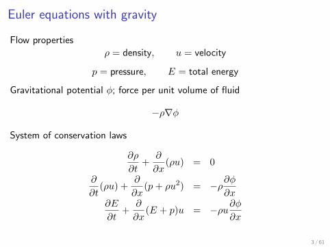
Euler equations with gravity
Flow properties
ρ = density, u = velocity
p = pressure, E = total energy
Gravitational potential φ; force per unit volume of fluid
−ρ∇φ
System of conservation laws
∂ρ
∂t+
∂
∂x(ρu) = 0
∂
∂t(ρu) +
∂
∂x(p+ ρu2) = −ρ∂φ
∂x∂E
∂t+
∂
∂x(E + p)u = −ρu∂φ
∂x
3 / 61

Euler equations with gravity
Perfect gas assumption
p = (γ − 1)
[E − 1
2ρu2
], γ =
cpcv> 1
In compact notation
∂q
∂t+∂f
∂x= −
0ρρu
∂φ∂x
where
q =
ρρuE
, f =
ρup+ ρu2
(E + p)u
4 / 61

Hydrostatic solutions
• Fluid at restue = 0
• Mass and energy equation satisfied
• Momentum equationdpedx
= −ρedφ
dx(1)
• Need additional assumptions to solve this equation
• Assume ideal gas and some temperature profile Te(x)
pe(x) = ρe(x)RTe(x), R = gas constant
integrate (1) to obtain
pe(x) = p0 exp
(−∫ x
x0
φ′(s)
RTe(s)ds
)5 / 61

Hydrostatic solutions• If the hydrostatic state is isothermal, i.e., Te(x) = Te = const, then
pe(x) exp
(φ(x)
RTe
)= const (2)
Density
ρe(x) =pe(x)
RTe• If the hydrostatic solution is polytropic then we have following
relations
peρ−νe = const, peT
− νν−1
e = const, ρeT− 1ν−1
e = const (3)
where ν > 1 is some constant. From (1) and (3), we obtain
νRTe(x)
ν − 1+ φ(x) = const (4)
E.g., pressure is
pe(x) = C1 [C2 − φ(x)]ν−1ν
6 / 61
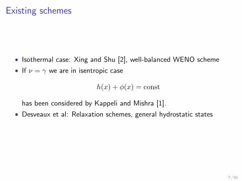
Existing schemes
• Isothermal case: Xing and Shu [2], well-balanced WENO scheme
• If ν = γ we are in isentropic case
h(x) + φ(x) = const
has been considered by Kappeli and Mishra [1].
• Desveaux et al: Relaxation schemes, general hydrostatic states
7 / 61
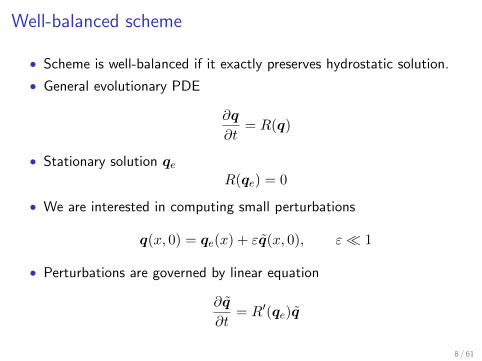
Well-balanced scheme
• Scheme is well-balanced if it exactly preserves hydrostatic solution.
• General evolutionary PDE
∂q
∂t= R(q)
• Stationary solution qeR(qe) = 0
• We are interested in computing small perturbations
q(x, 0) = qe(x) + εq(x, 0), ε 1
• Perturbations are governed by linear equation
∂q
∂t= R′(qe)q
8 / 61

Well-balanced scheme
• Some numerical scheme
∂qh∂t
= Rh(qh)
• qh,e = interpolation of qe onto the mesh
• Scheme is well balanced if
Rh(qh,e) = 0 =⇒ ∂qh∂t
= 0
• Suppose scheme is not well-balanced Rh(qh,e) 6= 0. Solution
qh(x, t) = qh,e(x) + εqh(x, t)
9 / 61
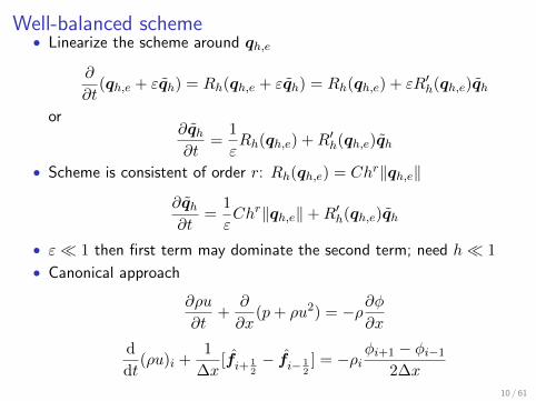
Well-balanced scheme• Linearize the scheme around qh,e
∂
∂t(qh,e + εqh) = Rh(qh,e + εqh) = Rh(qh,e) + εR′h(qh,e)qh
or∂qh∂t
=1
εRh(qh,e) +R′h(qh,e)qh
• Scheme is consistent of order r: Rh(qh,e) = Chr‖qh,e‖
∂qh∂t
=1
εChr‖qh,e‖+R′h(qh,e)qh
• ε 1 then first term may dominate the second term; need h 1
• Canonical approach
∂ρu
∂t+
∂
∂x(p+ ρu2) = −ρ∂φ
∂x
d
dt(ρu)i +
1
∆x[fi+ 1
2− fi− 1
2] = −ρi
φi+1 − φi−1
2∆x
10 / 61

Scope of present work
• Second order finite volume scheme
• Ideal gas model: well-balanced for both isothermal and polytropicsolutions
• Most numerical fluxes can be used
11 / 61

Source term [2]Define
ψ(x) = −∫ x
x0
φ′(s)
RT (s)ds, x0 is arbitrary
Then∂ψ
∂x= − ∂
∂x
∫ x
x0
φ′(s)
RT (s)ds = − φ′(x)
RT (x)
and∂
∂xexp(ψ(x)) = exp(ψ(x))
∂ψ
∂x= − exp(ψ(x))
φ′(x)
RT (x)
so that
−ρ(x)∂φ
∂x= p(x) exp(−ψ(x))
∂
∂xexp(ψ(x))
Euler equations
∂q
∂t+∂f
∂x=
0ppu
exp(−ψ(x))∂
∂xexp(ψ(x))
12 / 61
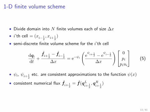
1-D finite volume scheme
• Divide domain into N finite volumes each of size ∆x
• i’th cell = (xi− 12, xi+ 1
2)
• semi-discrete finite volume scheme for the i’th cell
dqidt
+fi+ 1
2− fi− 1
2
∆x= e−ψi
(eψi+1
2 − eψi− 1
2
∆x
) 0pipiui
(5)
• ψi, ψi+ 12
etc. are consistent approximations to the function ψ(x)
• consistent numerical flux fi+ 12
= f(qLi+ 1
2
, qRi+ 1
2
)
13 / 61
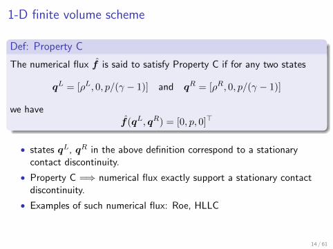
1-D finite volume scheme
Def: Property C
The numerical flux f is said to satisfy Property C if for any two states
qL = [ρL, 0, p/(γ − 1)] and qR = [ρR, 0, p/(γ − 1)]
we havef(qL, qR) = [0, p, 0]>
• states qL, qR in the above definition correspond to a stationarycontact discontinuity.
• Property C =⇒ numerical flux exactly support a stationary contactdiscontinuity.
• Examples of such numerical flux: Roe, HLLC
14 / 61

1-D finite volume scheme
• First order scheme
qLi+ 1
2
= qi, qRi+ 1
2
= qi+1
• Higher order scheme: To obtain the states qLi+ 1
2
, qRi+ 1
2
, reconstruct
the following set of variables
w =[ρe−ψ, u, pe−ψ
]>• Once wL
i+ 12
etc. are computed, the primitive variables are obtained as
ρLi+ 1
2
= eψi+1
2 (w1)Li+ 1
2
, uLi+ 1
2
= (w2)Li+ 1
2
, pLi+ 1
2
= eψi+1
2 (w3)Li+ 1
2
, etc.
15 / 61

Well-balanced property
Theorem
The finite volume scheme (5) together with a numerical flux whichsatisfies property C and reconstruction of w variables is well-balanced inthe sense that the initial condition given by
ui = 0, pi exp(−ψi) = const, ∀ i (6)
is preserved by the numerical scheme.
Proof: Start computation with an initial condition that satisfies (6). Sincewe reconstruct the variables w, at any interface i+ 1
2 we have
(w2)Li+ 1
2
= (w2)Ri+ 1
2
= 0, (w3)Li+ 1
2
= (w3)Ri+ 1
2
Hence
uLi+ 1
2
= uRi+ 1
2
= 0, pLi+ 1
2
= pRi+ 1
2
= pi exp(ψi+ 12− ψi) =: pi+ 1
2
16 / 61

Well-balanced property
and at i− 12
uLi− 1
2
= uRi− 1
2
= 0, pLi− 1
2
= pRi− 1
2
= pi exp(ψi− 12− ψi) =: pi− 1
2
Since the numerical flux satisfies property C, we have
fi− 12
= [0, pi− 12, 0]>, fi+ 1
2= [0, pi+ 1
2, 0]>
Mass and energy equations are already well balanced, i.e.,
dq(1)i
dt= 0,
dq(3)i
dt= 0
Momentum equation: on the left we have
f(2)
i+ 12
− f(2)
i− 12
∆x=pi+ 1
2− pi− 1
2
∆x
17 / 61

Well-balanced property
while on the right
pie−ψi e
ψi+1
2 − eψi− 1
2
∆x=pie
ψi+1
2−ψi − pie
ψi− 1
2−ψi
∆x=pi+ 1
2− pi− 1
2
∆x
and hence
dq(2)i
dt= 0
This proves that the initial condition is preserved under any timeintegration scheme.
18 / 61

Approximation of source term
• How to approximate ψi, ψi+ 12
, etc. ? Need some quadrature
• well-balanced property independent of quadrature rule to compute ψ.
• To preserve isothermal/polytropic solutions exactly, the quadraturerule has to be exact for these cases.
• To compute the source term in the i’th cell, we define the functionψ(x) as follows
ψ(x) = −∫ x
xi
φ′(s)
RT (s)ds
where we chose the reference position as xi.
19 / 61

Approximation of source term• To approximate the integrals we define the piecewise constant
temperature as follows
T (x) = Ti+ 12, xi < x < xi+1 (7)
where Ti+ 12
is the logarithmic average given by
Ti+ 12
=Ti+1 − Ti
log Ti+1 − log Ti
• The integrals are evaluated using the approximation of thetemperature given in (7) leading to the following expressions for ψ.
ψi = 0
ψi− 12
= − 1
RTi− 12
∫ xi− 1
2
xi
φ′(s)ds =φi − φi− 1
2
RTi− 12
ψi+ 12
= − 1
RTi+ 12
∫ xi+1
2
xi
φ′(s)ds =φi − φi+ 1
2
RTi+ 12
20 / 61

Approximation of source term
• Gravitational potential required at faces φi+ 12
• φ is governed by Poisson equation and hence is a smooth function.We can interpolate
φi+ 12
=1
2(φi + φi+1)
Sufficient to obtain second order accuracy. Then
ψi− 12
=φi − φi−1
2RTi− 12
, ψi = 0, ψi+ 12
=φi − φi+1
2RTi+ 12
(8)
21 / 61

Approximation of source term
Theorem
The source term discretization given by (8) is second order accurate.
Proof: The source term in (5) has the factor
e−ψieψi+1
2 − eψi− 1
2
∆x=
exp
(φi−φi+1
2RTi+1
2
)− exp
(φi−φi−1
2RTi− 1
2
)∆x
using (8)
Using a Taylor expansion around xi we get
1
Ti− 12
=1
Ti[1 +O(∆x2)],
1
Ti+ 12
=1
Ti[1 +O(∆x2)]
22 / 61
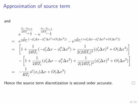
Approximation of source term
and
e
φi−φi+1
2RTi+1
2 − e
φi−φi−1
2RTi− 1
2
= e1
2RTi(−φ′i∆x−φ′′i ∆x2+O(∆x3)) − e
12RTi
(+φ′i∆x−φ′′i ∆x2+O(∆x3))
=
[1 +
1
2RTi(−φ′i∆x− φ′′i ∆x2) +
1
2(2RTi)2(φ′i∆x)2 +O(∆x3)
]−[1 +
1
2RTi(φ′i∆x− φ′′i ∆x2) +
1
2(2RTi)2(φ′i∆x)2 +O(∆x3)
]= − 1
RTiφ′(xi)∆x+O(∆x3)
Hence the source term discretization is second order accurate.
23 / 61

Theorem
Any hydrostatic solution which is isothermal or polytropic is exactlypreserved by the finite volume scheme (5).
Proof: Take initial condition to be a hydrostatic solution. We have toverify that the initial condition satisfies equation (6).
Isothermal case: Ti+ 12
= Te = const, and using (2) we obtain
pi+1e−ψi+1
pie−ψi=pi+1
pieψi−ψi+1 =
pi+1
piexp
(φi+1 − φiRTe
)=pi+1 exp(φi+1/RTe)
pi exp(φi/RTe)= 1
Polytropic case:
pi+1e−ψi+1
pie−ψi=pi+1
pieψi−ψi+1 =
pi+1
piexp
φi+1 − φiRTi+ 1
2
24 / 61
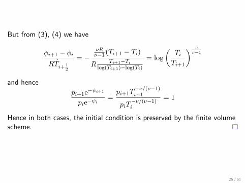
But from (3), (4) we have
φi+1 − φiRTi+ 1
2
= −νRν−1(Ti+1 − Ti)R Ti+1−Ti
log(Ti+1)−log(Ti)
= log
(TiTi+1
) νν−1
and hence
pi+1e−ψi+1
pie−ψi=pi+1T
−ν/(ν−1)i+1
piT−ν/(ν−1)i
= 1
Hence in both cases, the initial condition is preserved by the finite volumescheme.
25 / 61

Summary of the scheme
Using the approximations given by (8), the semi-discrete finite volumescheme is given by
dqidt
+fi+ 1
2− fi− 1
2
∆x=
eβi+1
2(φi−φi+1) − e
βi− 1
2(φi−φi−1)
∆x
0pipiui
where we have introduced the quantity
βi+ 12
=1
2RTi+ 12
As an example of reconstruction, we discuss the minmod-type scheme forthe interface i+ 1
2 which is given by
wLi+ 1
2
= wi +1
2m(θ(wi −wi−1), (wi+1 −wi−1)/2, θ(wi+1 −wi))
26 / 61

Summary of the scheme
wRi+ 1
2
= wi+1 −1
2m(θ(wi+1 −wi), (wi+2 −wi+1)/2, θ(wi+2 −wi+1))
where θ ∈ [1, 2] and m(·, ·, ·) is the minmod limiter function given by
m(a, b, c) =
smin(|a|, |b|, |c|) if s = sign(a) = sign(b) = sign(c)
0 otherwise
The variables w are defined using the potential relative to xi+ 12
ψ(x) = −∫ x
xi+1
2
φ′(s)
RT (s)ds
27 / 61

Summary of the schemeThen
ψi−1 =φi − φi−1
RTi− 12
+φi+ 1
2− φi
RTi+ 12
= 2βi− 12(φi − φi−1) + βi+ 1
2(φi+1 − φi)
ψi =φi+ 1
2− φi
RTi+ 12
= βi+ 12(φi+1 − φi)
ψi+1 = −φi+1 − φi+ 1
2
RTi+ 12
= −βi+ 12(φi+1 − φi)
ψi+2 = −φi+1 − φi+ 1
2
RTi+ 12
− φi+2 − φi+1
RTi+ 32
= −βi+ 12(φi+1 − φi)− 2βi+ 3
2(φi+2 − φi+1)
In terms of the above ψi’s, the variables w are defined as follows
wj =
ρje−ψjujpje−ψj
, j = i− 1, i, i+ 1, i+ 2
28 / 61

Summary of the scheme
Since ψi+ 12
= 0 we obtain the reconstructed values as
ρup
Li+ 1
2
= wLi+ 1
2
,
ρup
Ri+ 1
2
= wRi+ 1
2
For the first and last cells, we extrapolate the potential from inside thedomain to the faces located on the domain boundary
φ 12
=3
2φ1 −
1
2φ2, φN+ 1
2=
3
2φN −
1
2φN−1
29 / 61

Isothermal examples: well-balanced test
Density and pressure are given by
ρe(x) = pe(x) = exp(−φ(x))
N = 100, 1000, final time = 2
Potential 1 Potential 2 Potential 3
φ(x) x 12x
2 sin(2πx)
Table: Potential functions used for well-balanced tests
30 / 61

Isothermal examples: well-balanced test
Potential Cells Density Velocity Pressure
x 100 8.21676e-15 4.98682e-16 9.19209e-151000 8.00369e-14 1.51719e-14 9.15152e-14
12x
2 100 1.01874e-14 2.49332e-16 1.06837e-141000 1.05202e-13 4.10434e-16 1.11861e-13
sin(2πx) 100 1.12466e-14 5.79978e-16 1.74966e-141000 1.16191e-13 2.93729e-15 1.76361e-13
Table: Error in density, velocity and pressure for isothermal example
31 / 61

Isentropic examples: well-balanced testIsentropic hydrostatic solution
Te(x) = 1− γ − 1
γφ(x), ρe = T
1γ−1e , pe = ργe
N = 100, 1000, final time = 2
Potential Cells Density Velocity Pressure
x 100 6.86395e-15 2.65535e-16 7.88869e-151000 7.03820e-14 7.79350e-16 8.03623e-14
12x
2 100 1.06604e-14 2.27512e-16 1.04128e-141000 1.10726e-13 1.15415e-15 1.09185e-13
sin(2πx) 100 1.27570e-14 5.18212e-16 1.65185e-141000 1.29020e-13 1.12837e-15 1.66566e-13
Table: Error in density, velocity and pressure for isentropic example
32 / 61

Polytropic examples: well-balanced test
Polytropic hydrostatic solutions
Te(x) = 1− ν − 1
νφ(x), ρe = T
1ν−1e , pe = ρνe
ν = 1.2, N = 100, 1000, final time = 2
Potential Cells Density Velocity Pressure
x 100 6.86395e-15 2.65535e-16 7.88869e-151000 7.03820e-14 7.79350e-16 8.03623e-14
12x
2 100 1.06604e-14 2.27512e-16 1.04128e-141000 1.10726e-13 1.15415e-15 1.09185e-13
sin(2πx) 100 1.27570e-14 5.18212e-16 1.65185e-141000 1.29020e-13 1.12837e-15 1.66566e-13
Table: Error in density, velocity and pressure for polytropic example
33 / 61

Non-isothermal example
• Stationary solution
φ(x) =1
2x2, ρe(x) = exp(−x), pe(x) = (1 + x) exp(−x)
• corresponds to a non-uniform temperature profile
Te(x) = 1 + x
• Neither isothermal nor polytropic; present scheme will not be able topreserve the exact hydrostatic solution
• Instead, we construct an approximation to the above hydrostaticsolution by numerically integrating the hydrostatic equations (1)
p1 = pe(x1), ρ1 =p1
RTe(x1)
pi = pi−1 exp(−2βi− 12(φi−φi−1)), ρi =
piRTe(xi)
, i = 2, 3, . . . , N
34 / 61
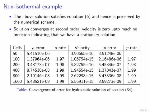
Non-isothermal example
• The above solution satisfies equation (6) and hence is preserved bythe numerical scheme.
• Solution converges at second order; velocity is zero upto machineprecision indicating that we have a stationary solution
Cells ρ error ρ rate Velocity p error p rate
50 5.41510e-06 - 3.90665e-16 8.51248e-06100 1.37964e-06 1.97 1.06754e-15 2.16486e-06 1.97200 3.48173e-07 1.98 4.82755e-16 5.45846e-07 1.98400 8.74530e-08 1.99 1.94554e-15 1.37043e-07 1.99800 2.19146e-08 1.99 2.62298e-15 3.43336e-08 1.991600 5.48521e-09 1.99 6.56911e-15 8.59273e-09 1.99
Table: Convergence of error for hydrostatic solution of section (34).
35 / 61
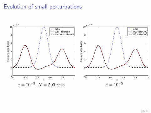
Evolution of small perturbations
The initial condition is taken to be the following
φ =1
2x2, u = 0, ρ(x) = exp(−φ(x))
Add small perturbation to equilibrium pressure
p(x) = exp(−φ(x)) + ε exp(−100(x− 1/2)2), 0 < ε 1
Non-well-balanced scheme
∂φ
∂x(xi) ≈
φi+1 − φi−1
2∆x, reconstruct ρ, u, p
Using exact derivative of potential does not improve results. In practice, φis only available at grid points.
36 / 61

Evolution of small perturbations
0 0.2 0.4 0.6 0.8 1−2
0
2
4
6
8
10x 10
−4
x
Pre
ssur
e pe
rtur
batio
n
InitialWell−balancedNon well−balanced
0 0.2 0.4 0.6 0.8 1−2
0
2
4
6
8
10x 10
−6
xP
ress
ure
pert
urba
tion
InitialWell−balancedNon well−balanced
ε = 10−3, N = 100 cells ε = 10−5, N = 100 cells
37 / 61
Evolution of small perturbations
0 0.2 0.4 0.6 0.8 1−2
0
2
4
6
8
10x 10
−6
x
Pre
ssur
e pe
rtur
batio
n
InitialWell−balancedNon well−balanced
0 0.2 0.4 0.6 0.8 1−2
0
2
4
6
8
10x 10
−6
xP
ress
ure
pert
urba
tion
InitialWB, cells=100WB, cells=500
ε = 10−5, N = 500 cells ε = 10−5
38 / 61

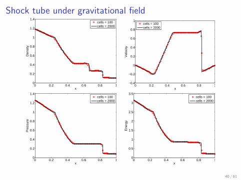
Shock tube under gravitational field
Gravitational field
φ(x) = x
The domain is [0, 1] and the initial conditions are given by
(ρ, u, p) =
(1, 0, 1) x < 1
2
(0.125, 0, 0.1) x > 12
Solid wall boundary conditions. Final time t = 0.2, N = 100, 2000 cells
39 / 61
Shock tube under gravitational field
0 0.2 0.4 0.6 0.8 10
0.2
0.4
0.6
0.8
1
1.2
1.4
x
Den
sity
cells = 100cells = 2000
0 0.2 0.4 0.6 0.8 1−0.4
−0.2
0
0.2
0.4
0.6
0.8
1
x
Vel
ocity
cells = 100cells = 2000
0 0.2 0.4 0.6 0.8 10
0.2
0.4
0.6
0.8
1
1.2
1.4
x
Pre
ssur
e
cells = 100cells = 2000
0 0.2 0.4 0.6 0.8 10
0.5
1
1.5
2
2.5
3
3.5
x
Ene
rgy
cells = 100cells = 2000
40 / 61
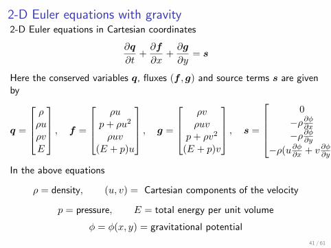
2-D Euler equations with gravity2-D Euler equations in Cartesian coordinates
∂q
∂t+∂f
∂x+∂g
∂y= s
Here the conserved variables q, fluxes (f , g) and source terms s are givenby
q =
ρρuρvE
, f =
ρu
p+ ρu2
ρuv(E + p)u
, g =
ρvρuv
p+ ρv2
(E + p)v
, s =
0
−ρ∂φ∂x−ρ∂φ∂y
−ρ(u∂φ∂x + v ∂φ∂y )
In the above equations
ρ = density, (u, v) = Cartesian components of the velocity
p = pressure, E = total energy per unit volume
φ = φ(x, y) = gravitational potential
41 / 61
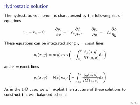
Hydrostatic solution
The hydrostatic equilibrium is characterized by the following set ofequations
ue = ve = 0,∂pe∂x
= −ρe∂φ
∂x,
∂pe∂y
= −ρe∂φ
∂y
These equations can be integrated along y = const lines
pe(x, y) = a(y) exp
(−∫ x
x0
φx(s, y)
RT (s, y)ds
)and x = const lines
pe(x, y) = b(x) exp
(−∫ y
y0
φy(x, s)
RT (x, s)ds
)As in the 1-D case, we will exploit the structure of these solutions toconstruct the well-balanced scheme.
42 / 61
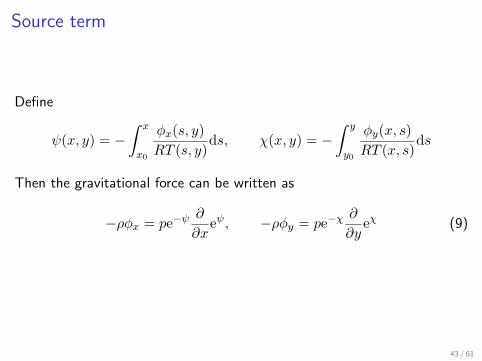
Source term
Define
ψ(x, y) = −∫ x
x0
φx(s, y)
RT (s, y)ds, χ(x, y) = −
∫ y
y0
φy(x, s)
RT (x, s)ds
Then the gravitational force can be written as
−ρφx = pe−ψ∂
∂xeψ, −ρφy = pe−χ
∂
∂yeχ (9)
43 / 61
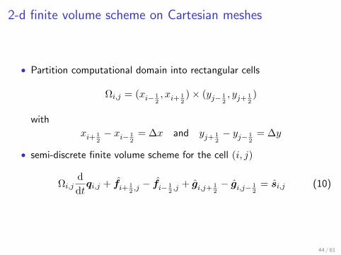
2-d finite volume scheme on Cartesian meshes
• Partition computational domain into rectangular cells
Ωi,j = (xi− 12, xi+ 1
2)× (yj− 1
2, yj+ 1
2)
with
xi+ 12− xi− 1
2= ∆x and yj+ 1
2− yj− 1
2= ∆y
• semi-discrete finite volume scheme for the cell (i, j)
Ωi,jd
dtqi,j + fi+ 1
2,j − fi− 1
2,j + gi,j+ 1
2− gi,j− 1
2= si,j (10)
44 / 61
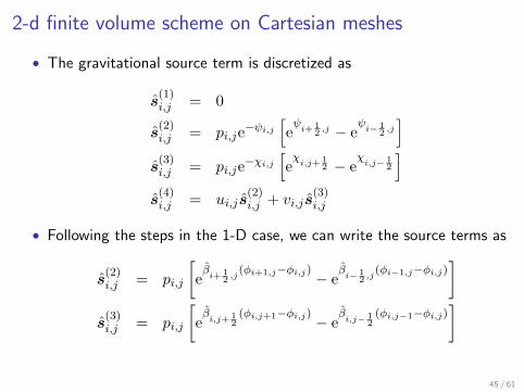
2-d finite volume scheme on Cartesian meshes
• The gravitational source term is discretized as
s(1)i,j = 0
s(2)i,j = pi,je
−ψi,j[eψi+1
2 ,j − eψi− 1
2 ,j
]s
(3)i,j = pi,je
−χi,j[eχi,j+1
2 − eχi,j− 1
2
]s
(4)i,j = ui,j s
(2)i,j + vi,j s
(3)i,j
• Following the steps in the 1-D case, we can write the source terms as
s(2)i,j = pi,j
[eβi+1
2 ,j(φi+1,j−φi,j) − e
βi− 1
2 ,j(φi−1,j−φi,j)
]s
(3)i,j = pi,j
[eβi,j+1
2(φi,j+1−φi,j) − e
βi,j− 1
2(φi,j−1−φi,j)
]
45 / 61
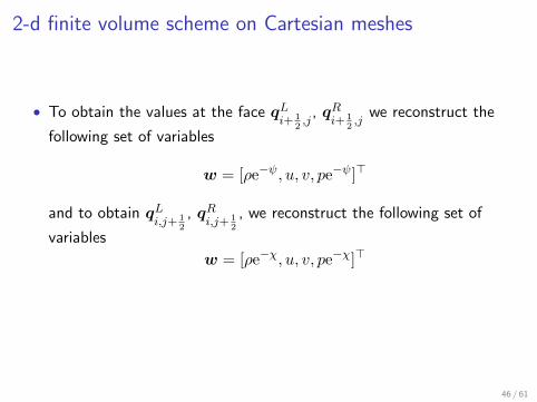
2-d finite volume scheme on Cartesian meshes
• To obtain the values at the face qLi+ 1
2,j
, qRi+ 1
2,j
we reconstruct the
following set of variables
w = [ρe−ψ, u, v, pe−ψ]>
and to obtain qLi,j+ 1
2
, qRi,j+ 1
2
, we reconstruct the following set of
variables
w = [ρe−χ, u, v, pe−χ]>
46 / 61
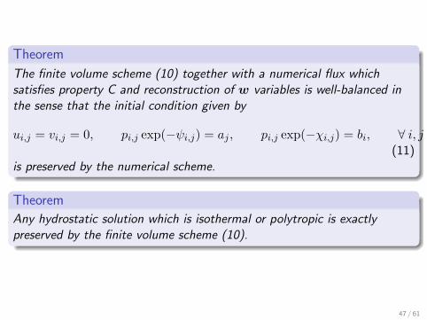
Theorem
The finite volume scheme (10) together with a numerical flux whichsatisfies property C and reconstruction of w variables is well-balanced inthe sense that the initial condition given by
ui,j = vi,j = 0, pi,j exp(−ψi,j) = aj , pi,j exp(−χi,j) = bi, ∀ i, j(11)
is preserved by the numerical scheme.
Theorem
Any hydrostatic solution which is isothermal or polytropic is exactlypreserved by the finite volume scheme (10).
47 / 61
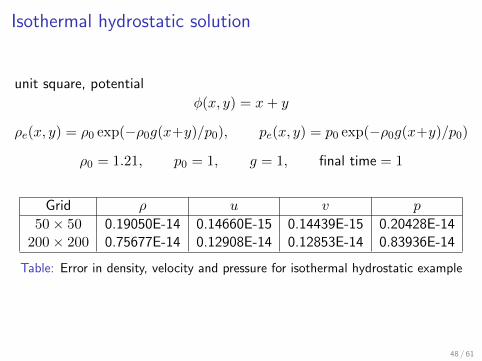
Isothermal hydrostatic solution
unit square, potential
φ(x, y) = x+ y
ρe(x, y) = ρ0 exp(−ρ0g(x+y)/p0), pe(x, y) = p0 exp(−ρ0g(x+y)/p0)
ρ0 = 1.21, p0 = 1, g = 1, final time = 1
Grid ρ u v p
50× 50 0.19050E-14 0.14660E-15 0.14439E-15 0.20428E-14200× 200 0.75677E-14 0.12908E-14 0.12853E-14 0.83936E-14
Table: Error in density, velocity and pressure for isothermal hydrostatic example
48 / 61

Isothermal hydrostatic solution
To study the accuracy of the scheme, we add an initial perturbation to thepressure and take the following initial condition
p(x, y, 0) = p0 exp(−ρ0g(x+y)/p0)+η exp(−100ρ0g((x−0.3)2+(y−0.3)2)/p0)
mesh = 50× 50, transmissive bc, final time = 0.15
pressure perturbation with η = 0.1
49 / 61
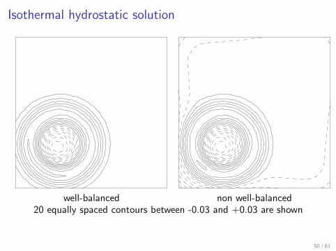
Isothermal hydrostatic solution
well-balanced non well-balanced20 equally spaced contours between -0.03 and +0.03 are shown
50 / 61
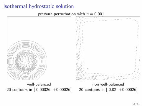
Isothermal hydrostatic solution
pressure perturbation with η = 0.001
well-balanced non well-balanced20 contours in [-0.00026, +0.00026] 20 contours in [-0.02, +0.00026]
51 / 61

Polytropic hydrostatic solution
Unit square, potential φ(x, y) = x+ y
Te = 1− ν − 1
ν(x+ y), pe = T
νν−1e , ρe = T
1ν−1e
ν = 1.2, final time = 1
Grid ρ u v p
50× 50 0.20449E-14 0.41148E-15 0.39802E-15 0.24637E-14200× 200 0.83747E-14 0.18037E-14 0.17986E-14 0.10107E-13
Table: Error in density, velocity and pressure
52 / 61

Polytropic hydrostatic solution
Perturbation of the initial pressure from the above polytropic solution
p(x, y, 0) = pe(x, y) + η exp(−100ρ0g((x− 0.3)2 + (y − 0.3)2)/p0)
mesh = 50× 50, transmissive bc, final time = 0.15
pressure perturbation with η = 0.1
53 / 61
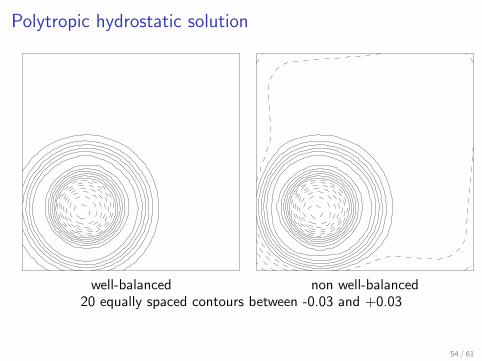
Polytropic hydrostatic solution
well-balanced non well-balanced20 equally spaced contours between -0.03 and +0.03
54 / 61

Polytropic hydrostatic solution
pressure perturbation with η = 0.001
well-balanced non well-balanced20 contours in [-0.00025,+0.00025] 20 contours in [-0.015,+0.0003]
55 / 61

Rayleigh-Taylor instability
• isothermal radial solution with potential φ = r: ρ = p = exp(−r)• Add perturbation: initial pressure and density are given by
p =
e−r r ≤ r0
e−rα
+r0(1−α)α r > r0
, ρ =
e−r r ≤ ri1αe−
rα
+r0(1−α)α r > ri
ri = r0(1 + η cos(kθ)), α = exp(−r0)/(exp(−r0) + ∆ρ)
• density jumps by an amount ∆ρ > 0 at interface r = ri, pressure iscontinuous.
∆ρ = 0.1, η = 0.02, k = 20, mesh = 240× 240 cells
domain = [−1,+1]× [−1,+1].
56 / 61
Rayleigh-Taylor instability
• In the regions r < r0(1− η) and r > r0(1 + η) the initial condition isin stable equilibrium
• but due to the discontinuous density, a Rayleigh-Taylor instabilitydevelops near interface defined by r = ri.
• Due to well-balanced scheme, instability is concentrated only aroundthe discontinuous interface
57 / 61

Rayleigh-Taylor instability
t = 0 t = 2.9
t = 3.8 t = 5.0
58 / 61
Extensions, ongoing work• 2/3-D curvilinear meshes• General equation of state, e.g., ideal gas with radiation pressure
p = ρRT +1
3aT 4
No exact hydrostatic solutions known, preserve an approximatehydrostatic solution
• Weak formulation
find u ∈ V such that a(u, v) = `(v) ∀v ∈ V• Galerkin method
find uh ∈ Vh such that a(uh, vh) = `(vh) ∀vh ∈ VhIn practice
find uh ∈ Vh such that ah(uh, vh) = `h(vh) ∀vh ∈ VhExact solution u is not a solution of above problem.
• Discontinuous Galerkin method: well-balanced for isothermalhydrostatic solution
59 / 61

Thank You
60 / 61

References
[1] R. Kappeli and S. Mishra, Well-balanced schemes for the Eulerequations with gravitation, J. Comput. Phys., 259 (2014),pp. 199–219.
[2] Yulong Xing and Chi-Wang Shu, High order well-balancedWENO scheme for the gas dynamics equations under gravitationalfields, J. Sci. Comput., 54 (2013), pp. 645–662.
61 / 61