COMPARISON OF EULER-EULER AND EULER-LAGRANGE APPROACH … B_Part2.pdf · COMPARISON OF EULER-EULER...
49
Third Serbian (28 th Yu) Congress on Theoretical and Applied Mechanics Vlasina lake, Serbia, 5-8 July 2011 B-08 COMPARISON OF EULER-EULER AND EULER-LAGRANGE APPROACH IN NUMERICAL SIMULATION OF MULTIPHASE FLOW IN VENTILATION MILL-AIR MIXING DUCT Kozic 1 , S. Ristic 2 , M. Puharic 2 , B. Katavic 2 1 Military Technical Institute Ratka Resanovica 1, Belgrade, Serbia e-mail: [email protected] 2 Institute Gosa, Milana Rakica 35, Belgrade Serbia e-mail: [email protected] Abstract. This paper presents the results of multiphase flow numerical simulations in ventilation mill and mixing duct with louvers separator of Kostolac B power plant. Due to very low volume fraction of the secondary solid phase, that is well below 10%, simulations are performed using both the mixture model of the Euler-Euler approach and Euler- Lagrange approach of ANSYS FLUENT software package. The gas mixture distribution at the main and secondary burner feed ducts obtained by the Euler-Euler mixture model is in a good agreement with the experiment. But aforementioned model also gives the same distribution of the pulverized coal at the burners, leading to large differences between the calculations and measurements. Because of that the Euler-Lagrange approach with Discrete Phase Model (DPM) is used where the fluid phase is treated as a continuum, while the dispersed solid phase is solved by tracking a large number of particles through the calculated flow field, i.e. computing the particle trajectories at specified intervals during the fluid phase calculation. Much better agreement of the calculated and measured value of the pulverized coal distribution at the burners is obtained using DPM. The tracking particles of the dispersed phase enables obtaining the influence of the louvers. It is noticed, in the numerical simulation, that due to the narrow gaps between the louvers only a small fraction of the pulverized coal passes through the gaps. The louvers actually act as an obstacle. The DPM model should be used in obtaining accurate distribution of the pulverized coal at the burners. 1. Introduction The world energy situation needs improvement of the economic performance of thermal plant by targeted modifications and future-oriented upgrades. Every contribution to the energy efficiency of thermal power plants, as an energy saving or an environmental protection is a significant result. A variety of theoretical, numerical, empirical and experimental methods are used in multidisciplinary researches of the ventilation mill-air duct systems of thermo plants [1- 18]. Measurement procedures of system parameters included: velocity distribution, temperature, pressure, pulverized coal and send particles concentration. Measurements are performed at different points, especially at burner’s distribution duct. Pitot probes, anemometers, thermo couples, gas analyzers, and others devices are used. Specific measurements conditions often cause failure of measuring equipment, so contactless measuring methods are introduced. 290
Transcript of COMPARISON OF EULER-EULER AND EULER-LAGRANGE APPROACH … B_Part2.pdf · COMPARISON OF EULER-EULER...
Third Serbian (28th Yu) Congress on Theoretical and Applied Mechanics Vlasina lake, Serbia, 5-8 July 2011 B-08
COMPARISON OF EULER-EULER AND EULER-LAGRANGE APPROACH IN NUMERICAL SIMULATION OF MULTIPHASE FLOW IN VENTILATION MILL-AIR MIXING DUCT
Kozic1, S. Ristic2, M. Puharic2, B. Katavic2
1 Military Technical Institute Ratka Resanovica 1, Belgrade, Serbia e-mail: [email protected]
2 Institute Gosa, Milana Rakica 35, Belgrade Serbia e-mail: [email protected]
Abstract. This paper presents the results of multiphase flow numerical simulations in ventilation mill and mixing duct with louvers separator of Kostolac B power plant. Due to very low volume fraction of the secondary solid phase, that is well below 10%, simulations are performed using both the mixture model of the Euler-Euler approach and Euler-Lagrange approach of ANSYS FLUENT software package. The gas mixture distribution at the main and secondary burner feed ducts obtained by the Euler-Euler mixture model is in a good agreement with the experiment. But aforementioned model also gives the same distribution of the pulverized coal at the burners, leading to large differences between the calculations and measurements. Because of that the Euler-Lagrange approach with Discrete Phase Model (DPM) is used where the fluid phase is treated as a continuum, while the dispersed solid phase is solved by tracking a large number of particles through the calculated flow field, i.e. computing the particle trajectories at specified intervals during the fluid phase calculation. Much better agreement of the calculated and measured value of the pulverized coal distribution at the burners is obtained using DPM. The tracking particles of the dispersed phase enables obtaining the influence of the louvers. It is noticed, in the numerical simulation, that due to the narrow gaps between the louvers only a small fraction of the pulverized coal passes through the gaps. The louvers actually act as an obstacle. The DPM model should be used in obtaining accurate distribution of the pulverized coal at the burners.
1. Introduction The world energy situation needs improvement of the economic performance of thermal plant by targeted modifications and future-oriented upgrades. Every contribution to the energy efficiency of thermal power plants, as an energy saving or an environmental protection is a significant result.
A variety of theoretical, numerical, empirical and experimental methods are used in multidisciplinary researches of the ventilation mill-air duct systems of thermo plants [1-18]. Measurement procedures of system parameters included: velocity distribution, temperature, pressure, pulverized coal and send particles concentration. Measurements are performed at different points, especially at burner’s distribution duct. Pitot probes, anemometers, thermo couples, gas analyzers, and others devices are used. Specific measurements conditions often cause failure of measuring equipment, so contactless measuring methods are introduced.
290
Third Serbian (28th Yu) Congress on Theoretical and Applied Mechanics Vlasina lake, Serbia, 5-8 July 2011 B-08
Numerical simulation of the flow is the most economical, fastest, and very reliable method in analyzing the complex issues of the multiphase flow and its optimization. Experimental investigation results are used as the input data and for numerical model verification. Verified model can be used for parametric analysis of the influence of, for example, gas phase velocity field, solid phase concentration and mass flow rate in the burner’s distribution channels, for different pulverized coal mass flow rate, geometry of flow separators and particle size distribution.
Ventilation mill is very important system and its operation has a significant influence on the level of power plant efficiency. The character of the multiphase flow in the ventilation mill and air mixing ducts, where recirculation gases, pulverized coal, sand and other materials are included, is directly related to the efficiency of plant.
Thermal Power Plant “Kostolc B”, total available capacity of 640 MW, consists of two blocks: block B1 in operation since 1987, block B2 in operation since 1991. There are two types of separators in the mixing duct, either louvers or centrifugal separator with adjustable blade angles. Some reconstructions have been accomplished with intention to optimize plant efficiency. This paper presents the results of numerical simulations of multiphase flow in the real system, Kostolac B power plant [1,9]. The flow through the mill duct systems with the lovers is considered. The results of the numerical simulations are compared with the measurements in the mill thermal plant [2,24,25].
Simulations are performed using both the mixture model of the Euler-Euler approach and Euler-Lagrange approach of ANSYS FLUENT software package. The gas mixture distribution at the main and secondary burner ducts obtained by the Euler-Euler mixture model is in a good agreement with the experiment, but large differences appear for the distribution of pulverized coal at the burners.
The Euler-Lagrange approach with Discrete Phase Model (DPM) is used to obtain real distribution of solid phase. The fluid phase is treated as a continuum, while the dispersed solid phase is solved by tracking a large number of particles through the flow field. The DPM model should be used in obtaining accurate distribution of the pulverized coal at the burners.
This paper presents the results of numerical simulations of multiphase flow in the real system, consisted of the ventilation mill and mixture channel of Drmno Kostolac B power plant [1, 9]. The flow through the mill duct systems with the louvers is considered. The results of the numerical simulations are compared with the measurements in the mill thermal plant.
2.Ventilation mill In Kostolac B power plant (total available capacity of 640 MW), the coal is pulverized in the ventilation mills. The system includes eight ventilation mills of EVT N 270.45 type, with a nominal capacity of 76 t / h of coal. Each mill is directly connected to the burner system consisted of four levels. Drying and transporting agent is the mixture of flue gas recirculation from the top of the furnace and primary pre heated air. After mills, the flue gas-coal particle mixture at the temperature in the range of 160-180 ºC passes through the
291
Third Serbian (28th Yu) Congress on Theoretical and Applied Mechanics Vlasina lake, Serbia, 5-8 July 2011 B-08
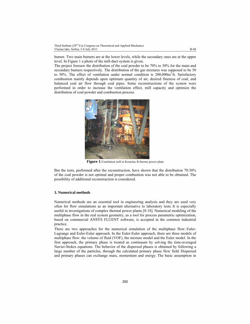
burner. Two main burners are at the lower levels, while the secondary ones are at the upper level. In Figure 1 a photo of the mill-duct system is given. The project foresaw the distribution of the coal powder to be 70% to 30% for the main and secondary burners respectively. The distribution of the gas mixtures was supposed to be 50 to 50%. The effect of ventilation under normal condition is 200,000m3/h. Satisfactory combustion mainly depends upon optimum quantity of air, desired fineness of coal, and balanced coal air flow through coal pipes. Some reconstructions of the system were performed in order to increase the ventilation effect, mill capacity and optimize the distribution of coal powder and combustion process.
Figure 1.Ventilation mill in Kostolac B thermo power plant
But the tests, performed after the reconstruction, have shown that the distribution 70:30% of the coal powder is not optimal and proper combustion was not able to be obtained. The possibility of additional reconstruction is considered. 3. Numerical methods Numerical methods are an essential tool in engineering analysis and they are used very often for flow simulations as an important alternative to laboratory tests. It is especially useful in investigations of complex thermal power plants [8-18]. Numerical modeling of the multiphase flow in the real system geometry, as a tool for process parametric optimization, based on commercial ANSYS FLUENT software, is accepted in the common industrial practice. There are two approaches for the numerical simulation of the multiphase flow: Euler-Lagrange and Euler-Euler approach. In the Euler-Euler approach, there are three models of multiphase flow: the volume of fluid (VOF), the mixture model and the Euler model. In the first approach, the primary phase is treated as continuum by solving the time-averaged Navier-Stokes equations. The behavior of the dispersed phases is obtained by following a large number of the particles, through the calculated primary phase flow field. Dispersed and primary phases can exchange mass, momentum and energy. The basic assumption in
292
Third Serbian (28th Yu) Congress on Theoretical and Applied Mechanics Vlasina lake, Serbia, 5-8 July 2011 B-08
this model is that the volume fraction of the dispersed, secondary phase is below 10-12%, although its mass can be even greater than the mass of the primary phase. The different phases in the Euler-Euler approach are considered as interpenetrating continua, thus introducing physic volume fractions as continuous functions of time and space. The sum for all phase’s volume fractions in each computational cell is equal to one. Conservation laws are applied to each phase. Constitutive relations obtained from empirical information must be added to close the set of equations. The mixture model is a simplified multiphase model that can be used in modeling flows where the phases move at different velocities using the concept of slip velocities, but the existence of local equilibrium at small length scales is assumed. This model can include n phases, where the equations of continuity, momentum and energy conservation are solved for the mixture, while the volume fraction equations are determined for each of the secondary phases. Algebraic equations are used in solving the relative velocities. This model enables selection of granular secondary phases and can be used as a good substitution for the full Euler multiphase model, in cases with wide size distribution of solid phase or when the interphase laws are unknown.
The Lagrange discrete phase model is based on the Euler-Lagrange approach where the fluid phase is treated as a continuum by solving the time-averaged Navier-Stokes equations, whereas the dispersed phase is solved by numerically integrating the equations of motion for the dispersed phase, i.e. computing the trajectories of a large number of particles or droplets through the calculated flow field. The dispersed phase consists of spherical particles that can exchange mass, momentum and energy with the fluid phase. Although the continuous phase acts on the dispersed phase through drag and turbulence while vice versa can be neglected, the coupling between the discrete and continuous phase can be included.
This paper presents the results of numerical simulations of multiphase flow in the real system, consisted of the ventilation mill and duct with the louver separator. The results of two methods (mixture and discrete phase model) for the numerical simulations are compared.
4. Numerical flow simulation
The results of the numerical simulation were obtained using the mixture model in the Euler-Euler approach and the Lagrange discrete phase model. In the mixture model the phases are allowed to be interpenetrating. The volume fractions in the control volume can have any value between 0 and 1. This model allows the phases to move with different velocities, using slip velocity between the phases. To describe particle motion in the fluid flow, all relevant forces have to be taken into account. The origin of the forces with continual effect is the presence and influence of the continual phase on the particles and the gravity [10-16]. The origins of the forces with impulse effect are the particle collision with the walls and obstacles and inter particle interactions. The intensity of the force that acts upon the particle depends on its shape. In most of the practical cases the shapes of the particles are irregular. In mathematical model and numerical calculations presented in this pa per particles are presented as ideal spheres.
293
Third Serbian (28th Yu) Congress on Theoretical and Applied Mechanics Vlasina lake, Serbia, 5-8 July 2011 B-08
The numerical modeling procedure of the multiphase flow in the ventilation mill and mixture channel is made up of two steps. The first step is geometry preparing and mesh generating. An unstructured tetrahedral grid consisted of 2996772 volume and 706444 surface elements is generated.
In the second step the flow field is calculated, after defining the general and multiphase model, phases and their interactions, viscous and turbulence model, boundary conditions, accuracy of numerical discretization, and initialization of the flow field. After obtaining solution convergence, post-processing and analysis of results were made.
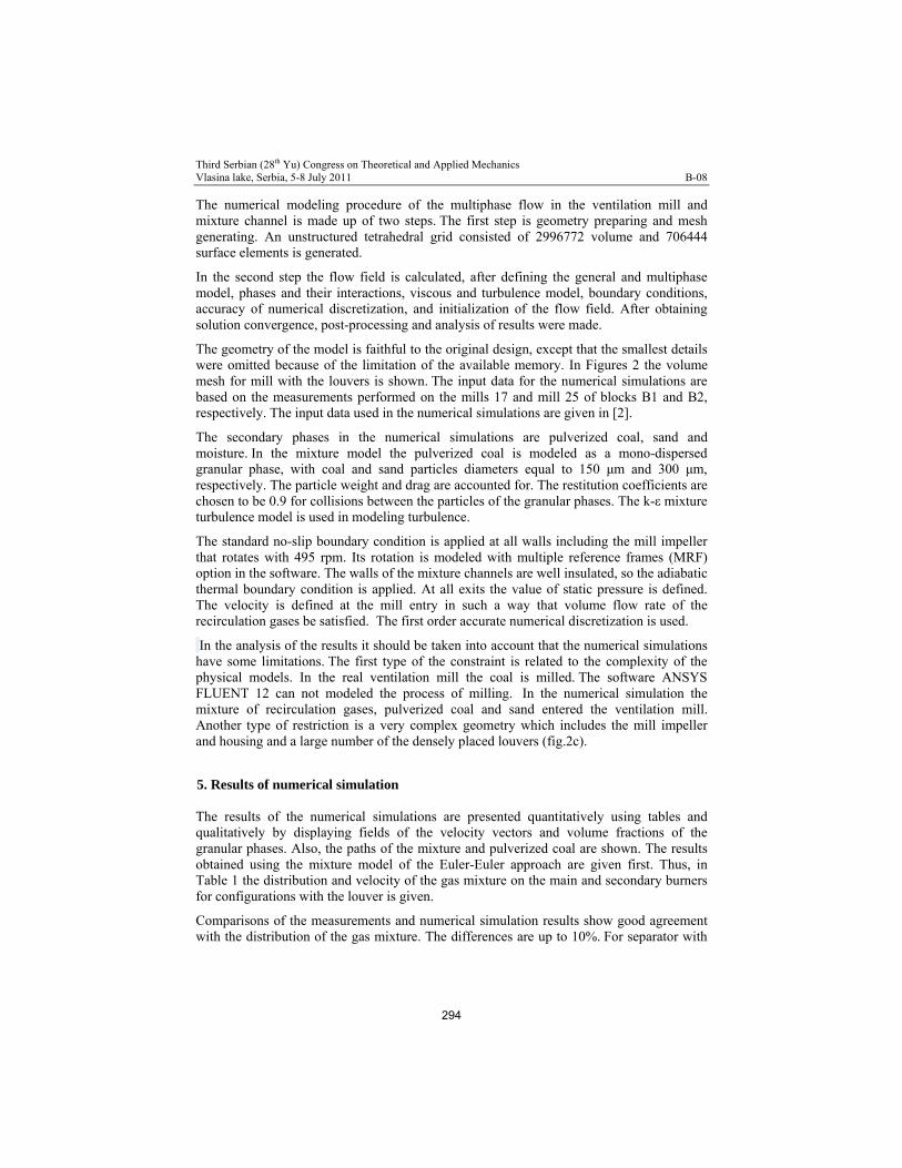
The geometry of the model is faithful to the original design, except that the smallest details were omitted because of the limitation of the available memory. In Figures 2 the volume mesh for mill with the louvers is shown. The input data for the numerical simulations are based on the measurements performed on the mills 17 and mill 25 of blocks B1 and B2, respectively. The input data used in the numerical simulations are given in [2].
The secondary phases in the numerical simulations are pulverized coal, sand and moisture. In the mixture model the pulverized coal is modeled as a mono-dispersed granular phase, with coal and sand particles diameters equal to 150 μm and 300 μm, respectively. The particle weight and drag are accounted for. The restitution coefficients are chosen to be 0.9 for collisions between the particles of the granular phases. The k-ε mixture turbulence model is used in modeling turbulence.
The standard no-slip boundary condition is applied at all walls including the mill impeller that rotates with 495 rpm. Its rotation is modeled with multiple reference frames (MRF) option in the software. The walls of the mixture channels are well insulated, so the adiabatic thermal boundary condition is applied. At all exits the value of static pressure is defined. The velocity is defined at the mill entry in such a way that volume flow rate of the recirculation gases be satisfied. The first order accurate numerical discretization is used.
In the analysis of the results it should be taken into account that the numerical simulations have some limitations. The first type of the constraint is related to the complexity of the physical models. In the real ventilation mill the coal is milled. The software ANSYS FLUENT 12 can not modeled the process of milling. In the numerical simulation the mixture of recirculation gases, pulverized coal and sand entered the ventilation mill. Another type of restriction is a very complex geometry which includes the mill impeller and housing and a large number of the densely placed louvers (fig.2c).
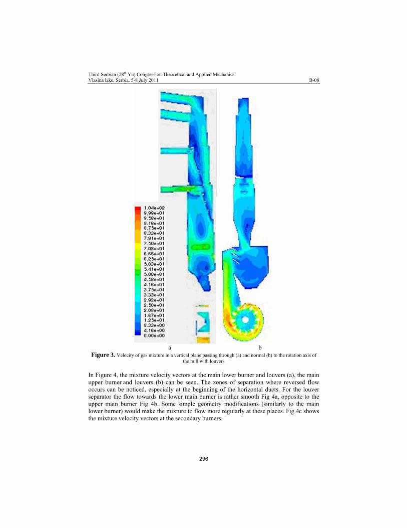
5. Results of numerical simulation The results of the numerical simulations are presented quantitatively using tables and qualitatively by displaying fields of the velocity vectors and volume fractions of the granular phases. Also, the paths of the mixture and pulverized coal are shown. The results obtained using the mixture model of the Euler-Euler approach are given first. Thus, in Table 1 the distribution and velocity of the gas mixture on the main and secondary burners for configurations with the louver is given.
Comparisons of the measurements and numerical simulation results show good agreement with the distribution of the gas mixture. The differences are up to 10%. For separator with
294
Third Serbian (28th Yu) Congress on Theoretical and Applied Mechanics Vlasina lake, Serbia, 5-8 July 2011 B-08
the louvers the gas mixture velocity is in very good agreement for the main lower burner and secondary upper burner, while for the main upper burner difference is about 28%.
a) b) c)
Figure 2. a-Volume mesh in the whole numerical domain for ventilation mill with louvers, b-Cross sections of volume mesh at lower louvers and exit to louver burner and upper louvers with upper burner duct, c) Surface grid
on several upper louvers
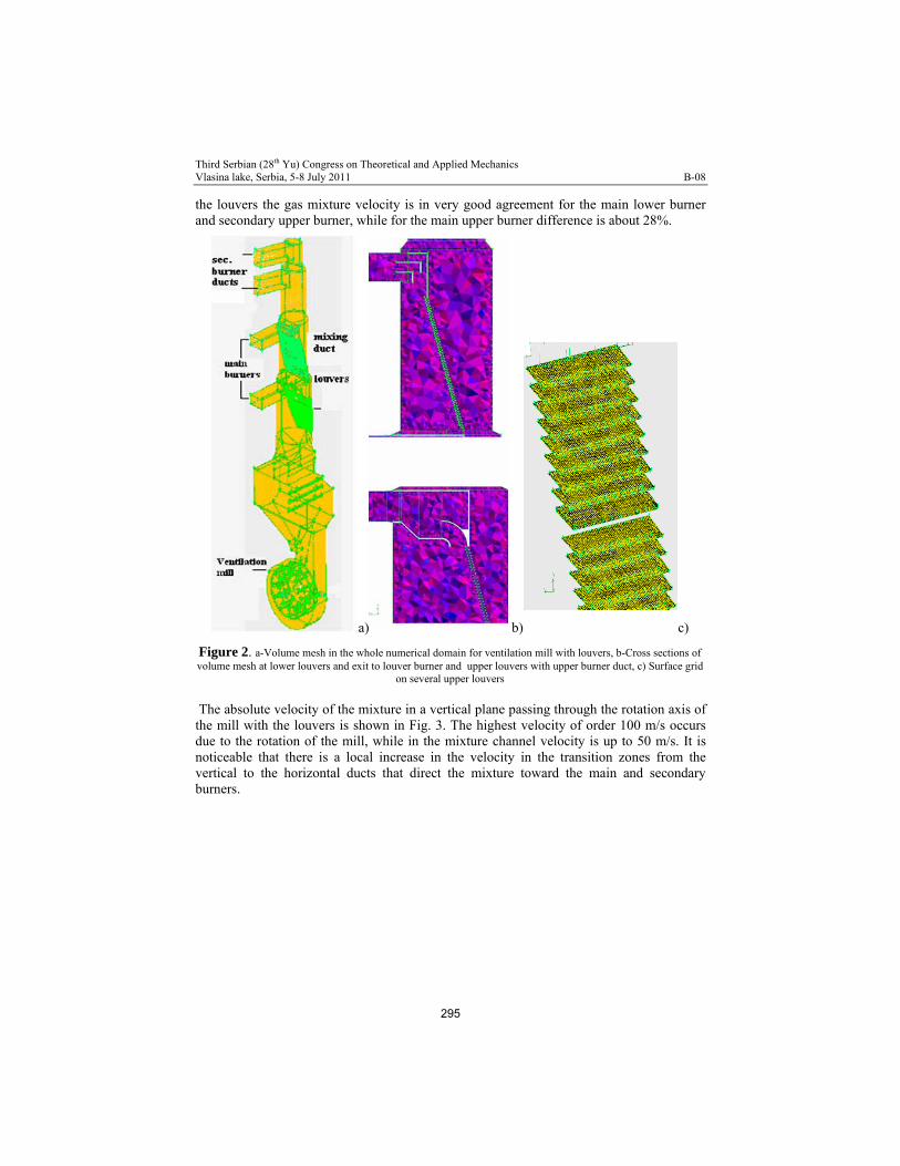
The absolute velocity of the mixture in a vertical plane passing through the rotation axis of the mill with the louvers is shown in Fig. 3. The highest velocity of order 100 m/s occurs due to the rotation of the mill, while in the mixture channel velocity is up to 50 m/s. It is noticeable that there is a local increase in the velocity in the transition zones from the vertical to the horizontal ducts that direct the mixture toward the main and secondary burners.
295
Third Serbian (28th Yu) Congress on Theoretical and Applied Mechanics Vlasina lake, Serbia, 5-8 July 2011 B-08
a b
Figure 3. Velocity of gas mixture in a vertical plane passing through (a) and normal (b) to the rotation axis of the mill with louvers
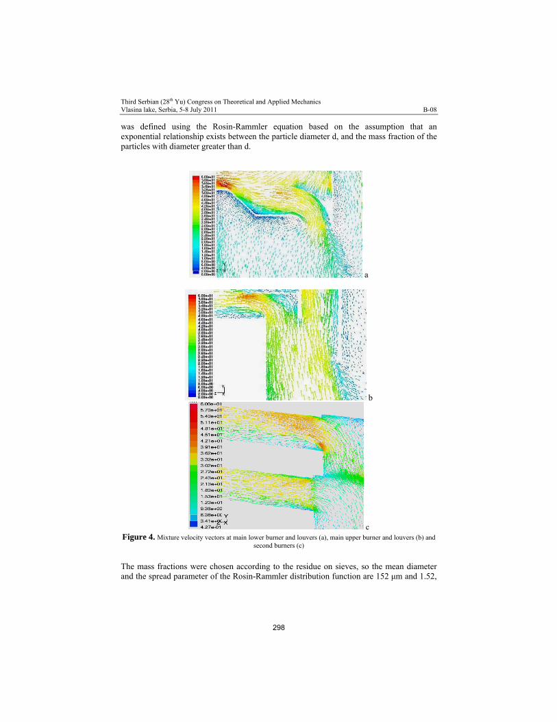
In Figure 4, the mixture velocity vectors at the main lower burner and louvers (a), the main upper burner and louvers (b) can be seen. The zones of separation where reversed flow occurs can be noticed, especially at the beginning of the horizontal ducts. For the louver separator the flow towards the lower main burner is rather smooth Fig 4a, opposite to the upper main burner Fig 4b. Some simple geometry modifications (similarly to the main lower burner) would make the mixture to flow more regularly at these places. Fig.4c shows the mixture velocity vectors at the secondary burners.
296
Third Serbian (28th Yu) Congress on Theoretical and Applied Mechanics Vlasina lake, Serbia, 5-8 July 2011 B-08
Table 1 Gas mixture distribution
Gas mixture distribution Velocity (m/s)
measurements [2]
numerical simulation
measurements [2]
numerical simulation
main lower burner 29 % 29.7 % 29.1 31.0
main upper burner 28 % 26.0 % 27.4 21.3
second lower burner 20 % 22.5 % 18.3 22.4
second upper burner 23 % 21.8 % 21.4 22.0
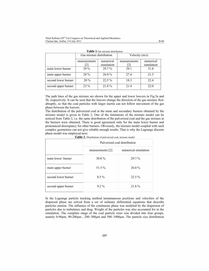
The path lines of the gas mixture are shown for the upper and lower louvers in Fig.5a and 5b, respectively. It can be seen that the louvers change the direction of the gas mixture flow abruptly, so that the coal particles with larger inertia can not follow movement of the gas phase between the louvers. The distribution of the pulverized coal at the main and secondary burners obtained by the mixture model is given in Table 2. One of the limitations of the mixture model can be noticed from Table 2, i.e. the same distribution of the pulverized coal and the gas mixture at the burners were obtained. There is good agreement only for the main lower burner and pronounced discrepancy for other burners. Obviously, the mixture model coupled with such complex geometries can not give reliable enough results. That is why the Lagrange discrete phase model was employed next.
Table 2. Distribution of pulverized coal, mixture model
Pulverized coal distribution
measurements [2] numerical simulation
main lower burner 30.8 % 29.7 %
main upper burner 51.5 % 26.0 %
second lower burner 8.5 % 22.5 %
second upper burner 9.2 % 21.8 %
In the Lagrange particle tracking method instantaneous positions and velocities of the dispersed phase are solved from a set of ordinary differential equations that describe particles motion. The influence of the continuous phase was modeled by the dispersion of particles due to turbulence and drag. Weight of the particles was also accounted for in the simulation. The complete range of the coal particle sizes was divided into four groups, namely 0-90μm, 90-200μm , 200–500μm and 500–1000μm. The particle size distribution
297
Third Serbian (28th Yu) Congress on Theoretical and Applied Mechanics Vlasina lake, Serbia, 5-8 July 2011 B-08
was defined using the Rosin-Rammler equation based on the assumption that an exponential relationship exists between the particle diameter d, and the mass fraction of the particles with diameter greater than d.
a
b
c Figure 4. Mixture velocity vectors at main lower burner and louvers (a), main upper burner and louvers (b) and
second burners (c)
The mass fractions were chosen according to the residue on sieves, so the mean diameter and the spread parameter of the Rosin-Rammler distribution function are 152 μm and 1.52,
298
Third Serbian (28th Yu) Congress on Theoretical and Applied Mechanics Vlasina lake, Serbia, 5-8 July 2011 B-08
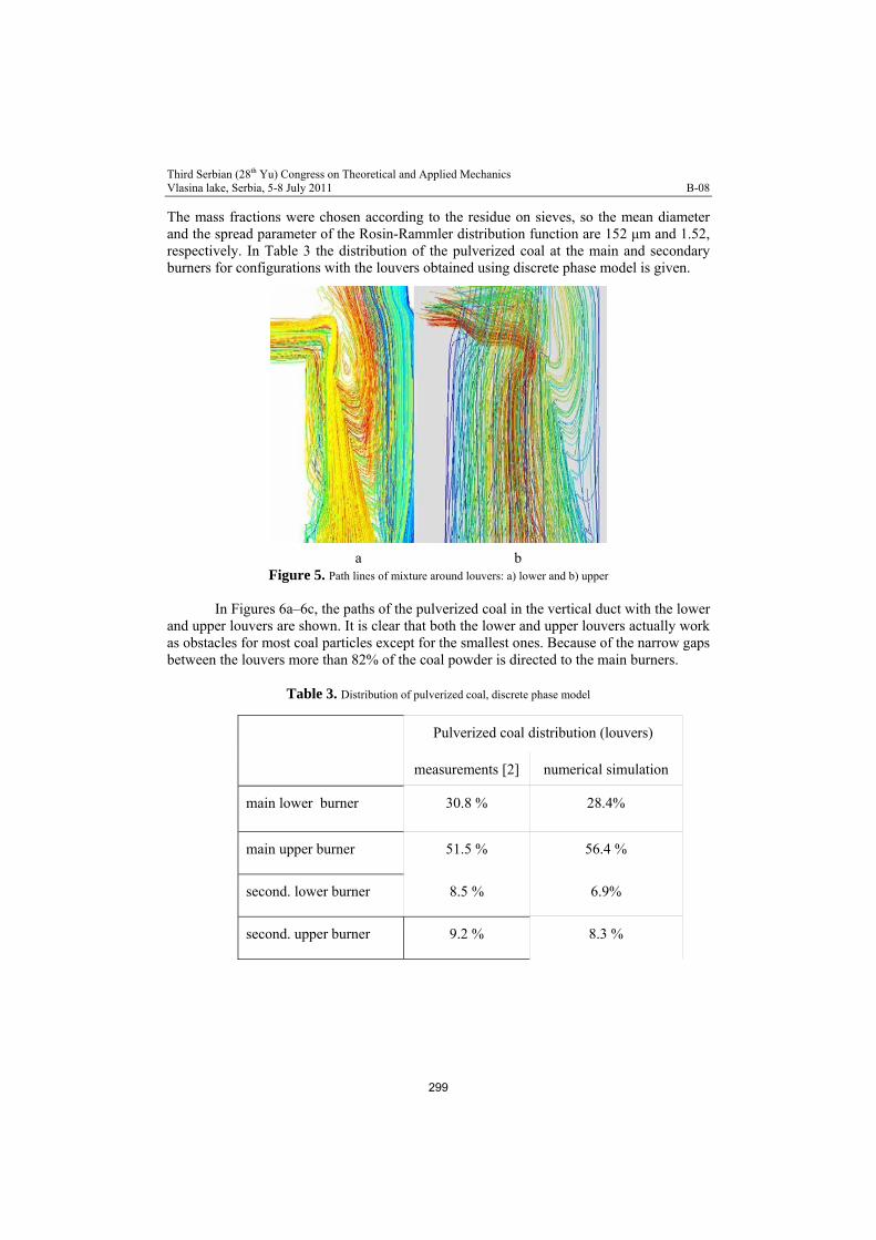
The mass fractions were chosen according to the residue on sieves, so the mean diameter and the spread parameter of the Rosin-Rammler distribution function are 152 μm and 1.52, respectively. In Table 3 the distribution of the pulverized coal at the main and secondary burners for configurations with the louvers obtained using discrete phase model is given.
a b Figure 5. Path lines of mixture around louvers: a) lower and b) upper
In Figures 6a–6c, the paths of the pulverized coal in the vertical duct with the lower and upper louvers are shown. It is clear that both the lower and upper louvers actually work as obstacles for most coal particles except for the smallest ones. Because of the narrow gaps between the louvers more than 82% of the coal powder is directed to the main burners.
Table 3. Distribution of pulverized coal, discrete phase model
Pulverized coal distribution (louvers)
measurements [2] numerical simulation
main lower burner 30.8 % 28.4%
main upper burner 51.5 % 56.4 %
second. lower burner 8.5 % 6.9%
second. upper burner 9.2 % 8.3 %
299
Third Serbian (28th Yu) Congress on Theoretical and Applied Mechanics Vlasina lake, Serbia, 5-8 July 2011 B-08
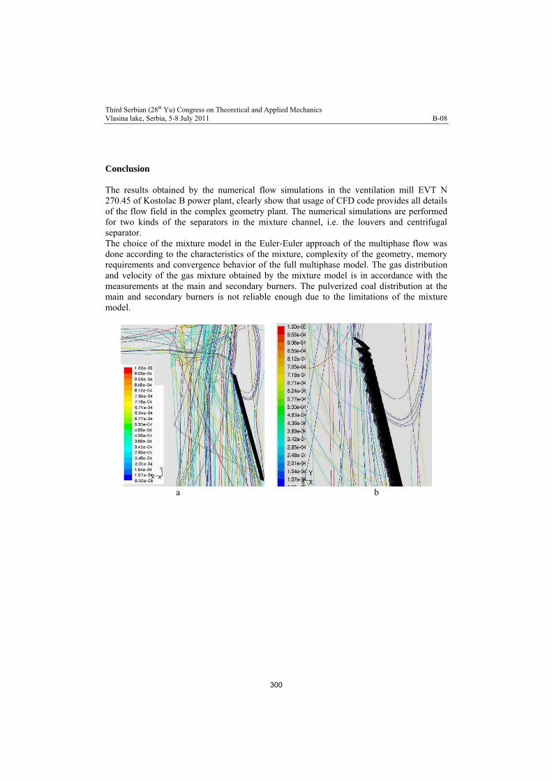
Conclusion The results obtained by the numerical flow simulations in the ventilation mill EVT N 270.45 of Kostolac B power plant, clearly show that usage of CFD code provides all details of the flow field in the complex geometry plant. The numerical simulations are performed for two kinds of the separators in the mixture channel, i.e. the louvers and centrifugal separator. The choice of the mixture model in the Euler-Euler approach of the multiphase flow was done according to the characteristics of the mixture, complexity of the geometry, memory requirements and convergence behavior of the full multiphase model. The gas distribution and velocity of the gas mixture obtained by the mixture model is in accordance with the measurements at the main and secondary burners. The pulverized coal distribution at the main and secondary burners is not reliable enough due to the limitations of the mixture model.
a b
300
Third Serbian (28th Yu) Congress on Theoretical and Applied Mechanics Vlasina lake, Serbia, 5-8 July 2011 B-08
c d
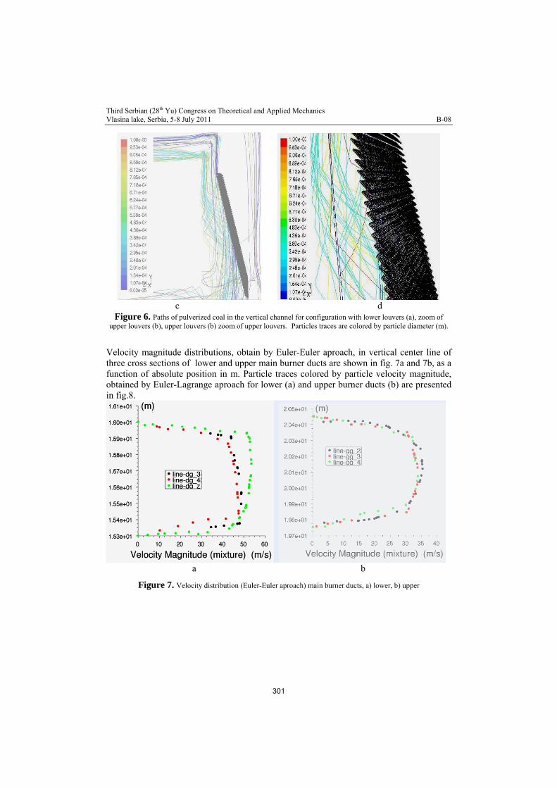
Figure 6. Paths of pulverized coal in the vertical channel for configuration with lower louvers (a), zoom of upper louvers (b), upper louvers (b) zoom of upper louvers. Particles traces are colored by particle diameter (m).
Velocity magnitude distributions, obtain by Euler-Euler aproach, in vertical center line of three cross sections of lower and upper main burner ducts are shown in fig. 7a and 7b, as a function of absolute position in m. Particle traces colored by particle velocity magnitude, obtained by Euler-Lagrange aproach for lower (a) and upper burner ducts (b) are presented in fig.8.
a b
Figure 7. Velocity distribution (Euler-Euler aproach) main burner ducts, a) lower, b) upper
301

Third Serbian (28th Yu) Congress on Theoretical and Applied Mechanics Vlasina lake, Serbia, 5-8 July 2011 B-08
a b
Figure 8. Particle traces colored by particle velocity magnitude: a) lower, b)upper burner ducts
Because of that, the Euler-Lagrange approach of the multiphase flow was finally used. The distribution of the coal obtained by the Lagrange particle tracking method agrees well with the measurements. The agreement is better for the centrifugal separator than the louver separator, because the influence of the former to the coal particles motion is considerably less. We have to point out that the results of the Lagrange particle tracking method are mostly dependent on the distribution of the coal particle sizes after milling. Acknowledgment: This work was financially supported by the Ministry of Science and Technological Development of Serbia under Project No. TR-34028. References: [1] Perković B., Mazurkijevič A., Tarasek V., Stević Lj., (2004), Reconstruction, and realization of the projected modrnization of power block B2 in the TE Costal, Termotehnika, 1, 30, pp.57-81 (in Serbian) [2] Thermo investigation and analysis of boiler plant blocks B1 and B2 in Costal TE, PD TENT Ltd. (2007, 2008), Production-technical sector, (internal study in Serbian), [3] Gulič M., Calculation of fan mill, Beograd, 1982 [4]Kuan B.T. Yang W., Solnordal C., (2003), CFD simulation and experiemental validation of delute particulate turbulent flows in 90º duct bend, Third International conferance on CFD in the minarals and process industries CSIRO, Melbourne, Australia, 10-12 dec., Proceedings, pp.531-536 [5] Kuan B.T., (2005), CFD simulation of dilute gas-solid two-phase flows with different solid size distributions in a curved 90º duct bend, 2005, ANZIAM J. C744-C763, [6] Lopez A.L., Oberkampf W.L., (1995), Numerical simulation of laminar flow in curved duct, SAND conference 95-0012C, 95-0130-6 [7] Tucakovic D. , Zivanovic T., Stevanovic V., Belosevic S., Galic R., (2008), A computer code for the prediction of mill gases and hot air distribution between burners’ sections at the utility boiler, Applied Thermal Engineering, 28, pp.2178–2186
302
Third Serbian (28th Yu) Congress on Theoretical and Applied Mechanics Vlasina lake, Serbia, 5-8 July 2011 B-08
[8] Belosevic S., Sijercic M., Tucakovic D., Crnomarkovic N., A numerical study of a utility boiler tangentially-fired furnace under different operating conditions, Fuel, 87, (2008), pp.3331–3338 [9] Liming Y., Smith A. C., (2008), Numerical study on effects of coal properties on spontaneous heating in longwall gob areas, Fuel, 87, pp.3409–3419 [10] Bhaster C., (2002), Numerical simulation of turbulent flow in complex geometries used in power plants, Advances in Engineering software, 33, pp.71-83 [11] Schiller L., Naumann Z., (1935),Ver.Deutch. Z., Ing., pp.77-318, [12] Drew D.A., Lahey R.T., (1993), In Particulate Two-Phase Flow, Butterworth-Heinemann, Boston, pp.509-566 [13] Baker B.J., Wainwright T.E., (1990), Studies in Molecular Dynamics II: Behaviour of a Small Number of Elastic Spheres, J.Chem.Phys., pp.33-439 [14] Chapman S., Cowling T.G., (1990), The Mathematical Theory of Non-Uniform Gases, Cambridge University Press, Cambridge, England, 3rd edition, [15] Morsi S.A., Alexander A.J., (1972), An Investigation of Particle Trajectories in Two-Phase Flow System, J. Fluid Mech., September 26, 1972, Proceedings.55, pp.193-208 [16] Wen C.Y., Yu Y.H., (1966), Mechanics of Fluidization, Chem.Eng.Prog.Symp. Series, 62, pp.100-111 [17] Živković G., Nemoda S., Stefanović, Radovanović P., (2009), Numerical simulation of the influence of stationary louver and coal P. particle size on distribution of pulverized coal to the feed ducts of a power plant burner, Thermal Science, Vol. 13, No. 4, pp. 79 – 90 [18] Živković N. V., Cvetinović D. B., Erić M. D., Marković Z. J., (2010), Numerical Analysis of the Flue Gas-Coal Particles mixture flow in burner’s distribution channels with regulation shutters at the tpp Nikola Tesla–a1 utility boiler, Thermal science, Vol. 14, No. 2, pp. 505-520
303

Third Serbian (28th Yu) Congress on Theoretical and Applied Mechanics Vlasina lake, Serbia, 5-8 July 2011 B-09
DETERMINATION OF THE AERODYNAMIC BRAKE EFFICIENCY FOR VARIOUS HIGH SPEED TRAIN VELOCITIES
S.Linic1, M.Puharic1, D.Matic1, V.Lucanin2 1 Institute Gosa, Milana Rakica 35, 11000 Belgrade
e-mail: [email protected] 2 Faculty of Mechanical Engineering, The University of Belgrade, Kraljice Marije 16, 11120 Belgrade
Abstract. This work is presenting the research results of the aerodynamic brake influence, mounted on the high-speed train’s roof, on the flow field and overall braking force. Aerodynamic brakes are designed in such way to generate braking force by means of increasing the aerodynamic drag by opened panels over the train. Train consists of two locomotives at each end and four passenger cars between, with 121m of gross length. Flow simulations were made by Fluent, for following configurations: clean train without the aerodynamic brakes; train configuration with one, two and three aerodynamic brakes. First brake panel was placed at a distance of 6m behind the train’s nose, the second panel at distance of 17m behind the first one and the third panel at a distance of 20m behind the second. At work, the analysis was made for the effect of serial interference that occurred as a consequence of the flow separation on the first aerodynamic brake. As the second brake is placed inside the first brake vortex trail, it generates lower drag and so the lower contribution to the overall drag force. Flow simulations are made for following velocities: 30 and 70 m/s, and the drag force per unit panel area was determined as a function of high speed train velocity and the brake position.
Keywords: aerodynamic brake, train, aerodynamic drag,
1. Introduction The aerodynamic brakes, designed in form of panels mounted over the roof of the high speed train, have a task to generate the drag force increasing the aerodynamic drag in open position. The brake that is in pullout (open) position blocks the air stream and causes the overpressure appearances in front of and under-pressure behind of braking panel. Pressure difference between in front and behind panel creates the drag force, normal to the panel surface. The tangential force, component caused by surface friction is negligible small in comparison to normal force, that presents braking force. As the aerodynamic drag is varying with the square of velocity, thus the braking force of aerodynamic brakes increases in a proportion to the square of velocity [1]. Flow field numerical simulations facilitate determination of the braking force intensity generated by the aerodynamic brakes. Flow simulation was done for half-model train (at
304

Third Serbian (28th Yu) Congress on Theoretical and Applied Mechanics Vlasina lake, Serbia, 5-8 July 2011 B-09
following text named train) by use of ANSYS Fluent 12.1 software. Flow space around the half-model was discredited by the tetrahedral mesh. Boundary conditions were defined over the boundaries of the numerical flow model of the cuboidical shape. In the near space all over the train body, the appropriate mesh elements were placed in the zone of the boundary layer. Largeness of the boundary layer mesh element was defined upon the condition of y+ = 30 for the first mesh element row close to the train body, with adequate 20% mesh element scale increment for every other mesh element row. Number of mesh elements for the train was 5 millions. Numerical flow simulations were performed for train velocities of 110 and 250km/h. Boundary conditions at the flow space input and output, in which simulations were done, were defined by pressures at those actual positions. All other boundary conditions were defined by the flow symmetry. Flow around the train was simulated as steady-state flow of the viscous incompressible fluid. The k – ε Realizable model of turbulence was applied with standard wall functions. The average number of iterations, needed for reaching of the result convergence was about 300 [4,5].
2. GEOMETRY OF THE TRAIN AND AERODYNAMIC BRAKES In this paper we discussed the train consist of two locomotives at ends and 4 passenger wagons between them. Over all length of the train composition was L=121m.
Figure 1. Train geometry and aerodynamic brakes positions
Each locomotive was 20m long, passenger wagons the same 20m long and the gaps between passengers wagons was 0.2m width. In Fig. 1.a train with aerodynamic brakes was shown. Near by, in Fig. 1.b, the first brake position was shown at the distance of 6m behind the train nose, and in Fig. 1.c the placement of second brake, which was placed at 17m behind the first one. The third brake was placed at a distance of 20m behind second brake.
3. THE AERODYNAMIC DRAG OF THE FLAT PLATE PLACED ORTHOGONALLY TO THE FREE STREAM
305
Third Serbian (28th Yu) Congress on Theoretical and Applied Mechanics Vlasina lake, Serbia, 5-8 July 2011 B-09
Here are discussed aerodynamic panels of rectangular shape, b=1.5m width and c=0.9m height. The drag coefficient for the flat plate, with dimension ration of 67.1cb was
Cx=1.14 [3,6,8]. As well known from the aerodynamic theory, aerodynamic drag per unit area being calculated from Eq. [3,8]:
2
2
2
1
m
NVC
A
FX
x
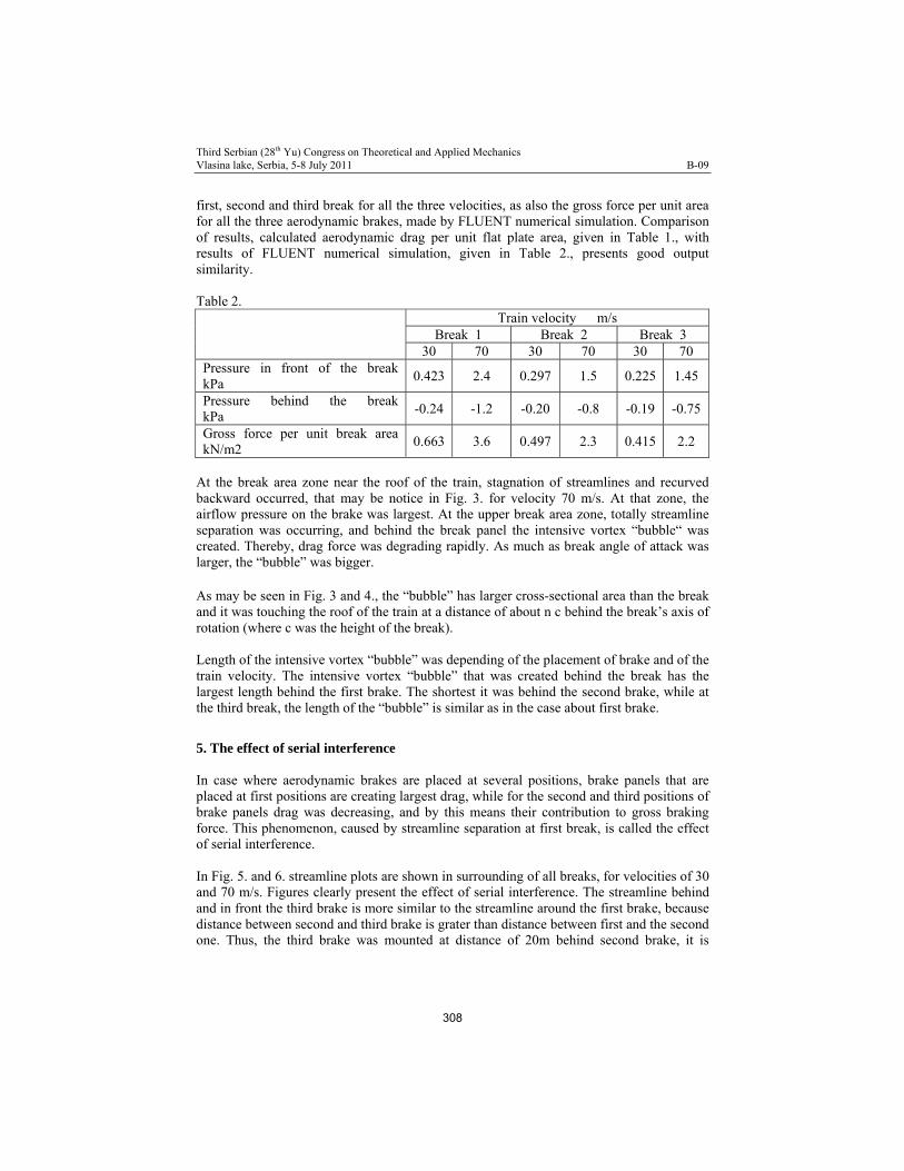
Calculation results for the aerodynamic drag per flat plate unit area, for velocities of V = 30, 50 and 70 m/s, are given in the Table 1. Table 1.
Gross force per break unit area ΔFx/A kN/m2 The number of panels n
Train velocity m/s
1 2 3 30 0.63 0.40 0.39 70 3.42 2.20 2.14
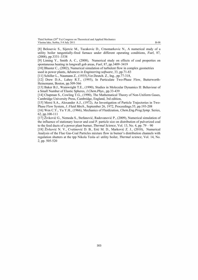
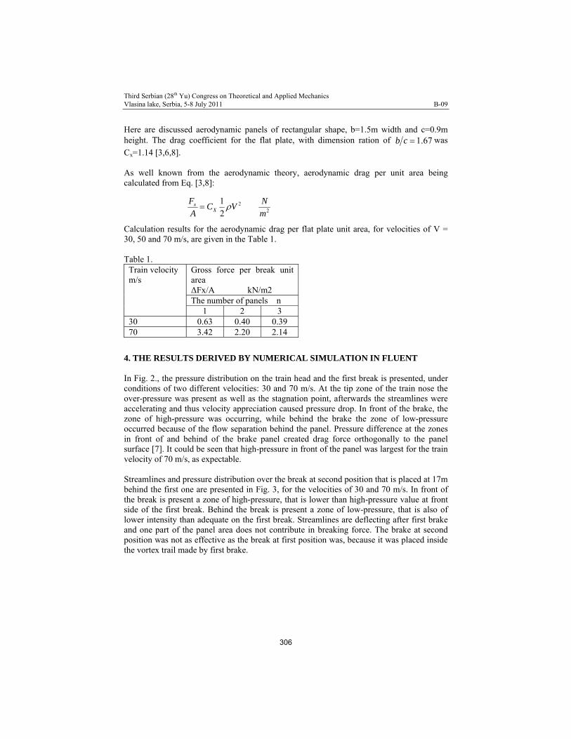
4. THE RESULTS DERIVED BY NUMERICAL SIMULATION IN FLUENT In Fig. 2., the pressure distribution on the train head and the first break is presented, under conditions of two different velocities: 30 and 70 m/s. At the tip zone of the train nose the over-pressure was present as well as the stagnation point, afterwards the streamlines were accelerating and thus velocity appreciation caused pressure drop. In front of the brake, the zone of high-pressure was occurring, while behind the brake the zone of low-pressure occurred because of the flow separation behind the panel. Pressure difference at the zones in front of and behind of the brake panel created drag force orthogonally to the panel surface [7]. It could be seen that high-pressure in front of the panel was largest for the train velocity of 70 m/s, as expectable. Streamlines and pressure distribution over the break at second position that is placed at 17m behind the first one are presented in Fig. 3, for the velocities of 30 and 70 m/s. In front of the break is present a zone of high-pressure, that is lower than high-pressure value at front side of the first break. Behind the break is present a zone of low-pressure, that is also of lower intensity than adequate on the first break. Streamlines are deflecting after first brake and one part of the panel area does not contribute in breaking force. The brake at second position was not as effective as the break at first position was, because it was placed inside the vortex trail made by first brake.
306
Third Serbian (28th Yu) Congress on Theoretical and Applied Mechanics Vlasina lake, Serbia, 5-8 July 2011 B-09
30 m/s 70 m/s
Figure 2. Pressure distribution at nose tip zone and on the first break at velocities of 30 and 70 m/s
30 m/s 70 m/s
Figure 3. Streamline plot and the pressure distribution around second break placed at 17m behind first brake, for the velocities of 30 and 70 m/s
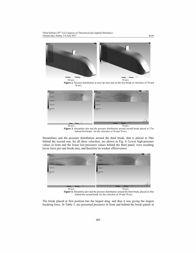
Streamlines and the pressure distribution around the third break, that is placed at 20m behind the second one, for all three velocities, are shown in Fig. 4. Lower high-pressure values in front and the lower low-pressures values behind the third panel, were resulting lower force per unit break area, and therefore its weaker effectiveness.
30 m/s 70 m/s
Figure 4. Streamline plot and the pressure distribution around the third break, placed at 20m behind the second break, for the velocities of 30 and 70 m/s
The break placed at first position has the largest drag, and thus it was giving the largest breaking force. In Table 2. are presented pressures in front and behind the break panels at
307
Third Serbian (28th Yu) Congress on Theoretical and Applied Mechanics Vlasina lake, Serbia, 5-8 July 2011 B-09
first, second and third break for all the three velocities, as also the gross force per unit area for all the three aerodynamic brakes, made by FLUENT numerical simulation. Comparison of results, calculated aerodynamic drag per unit flat plate area, given in Table 1., with results of FLUENT numerical simulation, given in Table 2., presents good output similarity. Table 2.
Train velocity m/s Break 1 Break 2 Break 3
30 70 30 70 30 70 Pressure in front of the break kPa
0.423 2.4 0.297 1.5 0.225 1.45
Pressure behind the break kPa
-0.24 -1.2 -0.20 -0.8 -0.19 -0.75
Gross force per unit break area kN/m2
0.663 3.6 0.497 2.3 0.415 2.2
At the break area zone near the roof of the train, stagnation of streamlines and recurved backward occurred, that may be notice in Fig. 3. for velocity 70 m/s. At that zone, the airflow pressure on the brake was largest. At the upper break area zone, totally streamline separation was occurring, and behind the break panel the intensive vortex “bubble“ was created. Thereby, drag force was degrading rapidly. As much as break angle of attack was larger, the “bubble” was bigger. As may be seen in Fig. 3 and 4., the “bubble” has larger cross-sectional area than the break and it was touching the roof of the train at a distance of about n c behind the break’s axis of rotation (where c was the height of the break). Length of the intensive vortex “bubble” was depending of the placement of brake and of the train velocity. The intensive vortex “bubble” that was created behind the break has the largest length behind the first brake. The shortest it was behind the second brake, while at the third break, the length of the “bubble” is similar as in the case about first brake.
5. The effect of serial interference In case where aerodynamic brakes are placed at several positions, brake panels that are placed at first positions are creating largest drag, while for the second and third positions of brake panels drag was decreasing, and by this means their contribution to gross braking force. This phenomenon, caused by streamline separation at first break, is called the effect of serial interference. In Fig. 5. and 6. streamline plots are shown in surrounding of all breaks, for velocities of 30 and 70 m/s. Figures clearly present the effect of serial interference. The streamline behind and in front the third brake is more similar to the streamline around the first brake, because distance between second and third brake is grater than distance between first and the second one. Thus, the third brake was mounted at distance of 20m behind second brake, it is
308
Third Serbian (28th Yu) Congress on Theoretical and Applied Mechanics Vlasina lake, Serbia, 5-8 July 2011 B-09
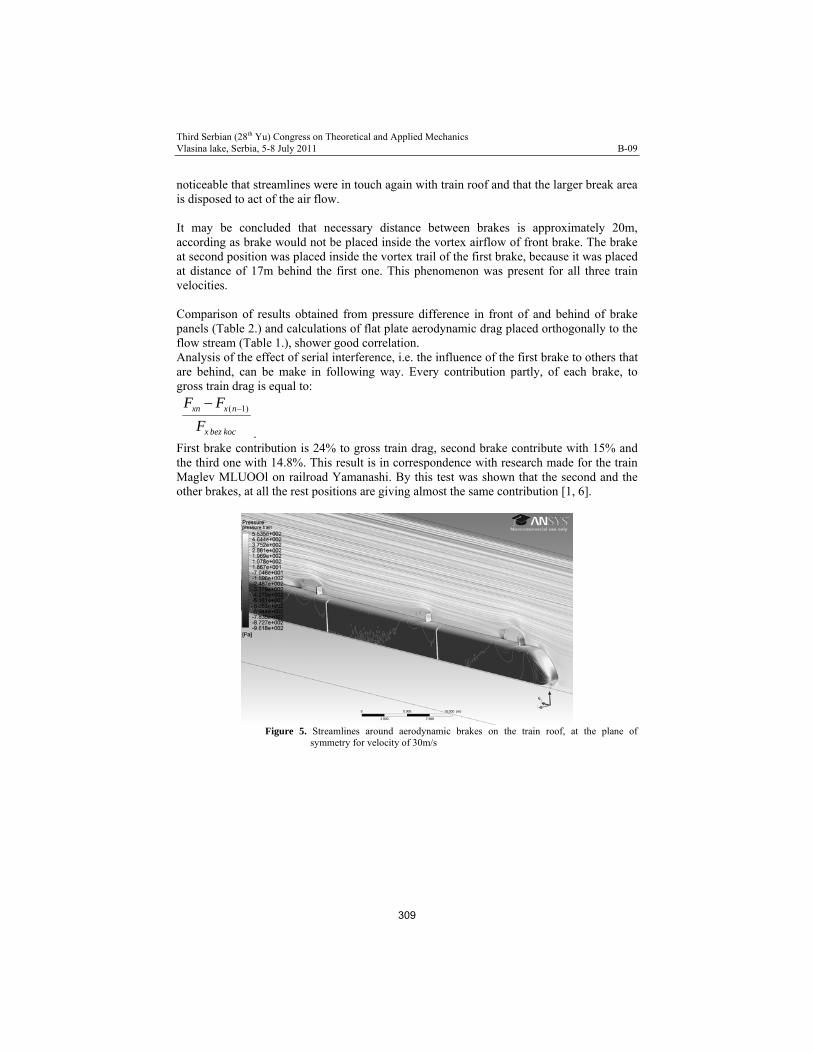
noticeable that streamlines were in touch again with train roof and that the larger break area is disposed to act of the air flow. It may be concluded that necessary distance between brakes is approximately 20m, according as brake would not be placed inside the vortex airflow of front brake. The brake at second position was placed inside the vortex trail of the first brake, because it was placed at distance of 17m behind the first one. This phenomenon was present for all three train velocities. Comparison of results obtained from pressure difference in front of and behind of brake panels (Table 2.) and calculations of flat plate aerodynamic drag placed orthogonally to the flow stream (Table 1.), shower good correlation. Analysis of the effect of serial interference, i.e. the influence of the first brake to others that are behind, can be make in following way. Every contribution partly, of each brake, to gross train drag is equal to:
( 1)xn x n
x bez koc
F F
F
. First brake contribution is 24% to gross train drag, second brake contribute with 15% and the third one with 14.8%. This result is in correspondence with research made for the train Maglev MLUOOl on railroad Yamanashi. By this test was shown that the second and the other brakes, at all the rest positions are giving almost the same contribution [1, 6].
Figure 5. Streamlines around aerodynamic brakes on the train roof, at the plane of
symmetry for velocity of 30m/s
309

Third Serbian (28th Yu) Congress on Theoretical and Applied Mechanics Vlasina lake, Serbia, 5-8 July 2011 B-09
Figure 6. Streamlines around aerodynamic brakes on the train roof, at the plane of
symmetry for velocity of 70m/s
6. Conclusion The force of the aerodynamic drag is proportional to the square of train velocity, thus pulling out of panels over the train can create a braking force with defined intensity, that become more significant by increasing the train velocity. The aerodynamic brakes like discussed can be used for trains at extremely urgent situations, when the imperative is rapid stopping. FLUENT flow simulations, for the train configuration with two locomotives at the ends and four passenger wagons in middle, for velocities of 30 and 70 m/s, for clear train and the train with one, two and three aerodynamic brakes over the train roof, have shown that high-pressure zones were arising behind the panel and the low-pressure zone in front of the panel, which were resulting the creation drag force on the break. For all the three brakes, dimensions of the intensive vortex “bubble”, behind the panel, was analyzed. It was noticed that the “bubble” length at first and third break are very the same, while the “bubble” behind the second brake has shorter length. This was caused by the fact that distance between first and second brakes was smaller than distance between second and third one. A dimension of the “bubble” depends also of train velocity. The “bubble“ was largest when the train velocity was highest (by 70m/s). It was also presented that braking panels, which are placed at first position, were creating the largest drag, while for panels at second and other positions drag force is decreasing, and by that means their contribution to braking force. At the first brake, the separation of air streamlines was occurring so the second brake was implicated by vortex trail of the first brake.
310
Third Serbian (28th Yu) Congress on Theoretical and Applied Mechanics Vlasina lake, Serbia, 5-8 July 2011 B-09
Acknowledgments. This paper was a result of research realized by the project of the the Ministry of Science and Technological Development, Republic of Serbia TR-35045, 2011-2014.
References [1] Yoshimura M., Saito S., Hosaka S., Tsunoda H (jun 2000.) Characteristics of the Aerodynamic Brake of the
Vehicle on the Yamanashi Maglev Test Line, QR of RTRI, vol.41, No.2. [2] Puharić, M. (2009.) The Model of Aerodynamic Research for High Speed Trains, PhD Thesis, Zrenjanin. [3] Anderson, J.D. (1996.) Fundamentals of aerodynamics, McGraw-Hill, inc. [4] H.K.Veersteg, W. Malalasekera (1995.): An Introduction to computational fluid dynamics – The finite volume
method, Longman. [5] J. Blazek (2001.) Computational Fluid Dynamics – Principles and Applications, Elsevier, [6] Puharić, M., Lučanin, V., Ristić, S., Linić, S. (2010.) Primena aerodinamičkih kočnica na vozove, Istraživanja
i projektovanja za privredu, ISSN 1451-4117, UDC 33, 8(2010)1, 168, pp.13-21, [7] Puharić, M., Adamović, Ž. (2008.) Research of high speed trains in the subsonic wind tunnel- Strojarstvo, No
50 (3), ISSN 0562-1887, UDK629.4.016.54.624.191:533.6, pp.151-160, [8] Rebuffet, P. (1969.) Aerodynamique experimentale, tome 1, Dunod, Paris,
311
Third Serbian (28th Yu) Congress on Theoretical and Applied Mechanics Vlasina lake, Serbia, 5-8 July 2011 B-11
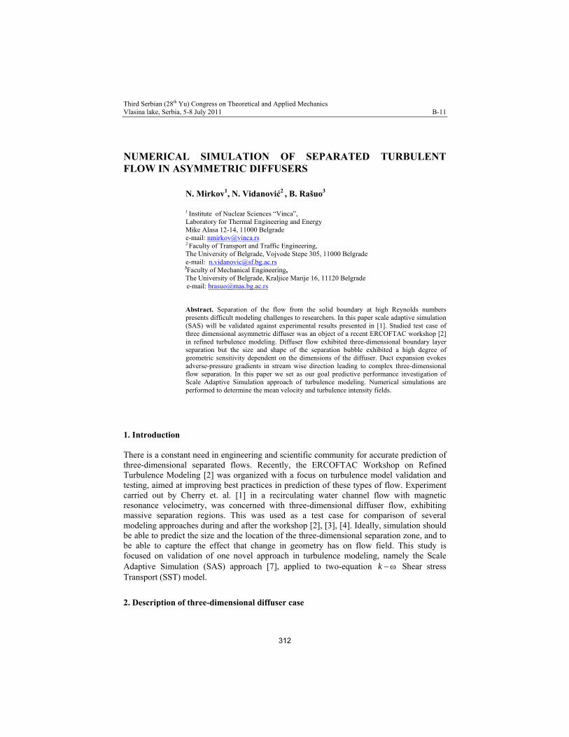
NUMERICAL SIMULATION OF SEPARATED TURBULENT FLOW IN ASYMMETRIC DIFFUSERS
N. Mirkov1, N. Vidanović2 , B. Rašuo3
1 Institute of Nuclear Sciences “Vinca”, Laboratory for Thermal Engineering and Energy Mike Alasa 12-14, 11000 Belgrade e-mail: [email protected] 2 Faculty of Transport and Traffic Engineering, The University of Belgrade, Vojvode Stepe 305, 11000 Belgrade e-mail: [email protected]
3Faculty of Mechanical Engineering, The University of Belgrade, Kraljice Marije 16, 11120 Belgrade
e-mail: [email protected]
Abstract. Separation of the flow from the solid boundary at high Reynolds numbers presents difficult modeling challenges to researchers. In this paper scale adaptive simulation (SAS) will be validated against experimental results presented in [1]. Studied test case of three dimensional asymmetric diffuser was an object of a recent ERCOFTAC workshop [2] in refined turbulence modeling. Diffuser flow exhibited three-dimensional boundary layer separation but the size and shape of the separation bubble exhibited a high degree of geometric sensitivity dependent on the dimensions of the diffuser. Duct expansion evokes adverse-pressure gradients in stream wise direction leading to complex three-dimensional flow separation. In this paper we set as our goal predictive performance investigation of Scale Adaptive Simulation approach of turbulence modeling. Numerical simulations are performed to determine the mean velocity and turbulence intensity fields.
1. Introduction There is a constant need in engineering and scientific community for accurate prediction of three-dimensional separated flows. Recently, the ERCOFTAC Workshop on Refined Turbulence Modeling [2] was organized with a focus on turbulence model validation and testing, aimed at improving best practices in prediction of these types of flow. Experiment carried out by Cherry et. al. [1] in a recirculating water channel flow with magnetic resonance velocimetry, was concerned with three-dimensional diffuser flow, exhibiting massive separation regions. This was used as a test case for comparison of several modeling approaches during and after the workshop [2], [3], [4]. Ideally, simulation should be able to predict the size and the location of the three-dimensional separation zone, and to be able to capture the effect that change in geometry has on flow field. This study is focused on validation of one novel approach in turbulence modeling, namely the Scale Adaptive Simulation (SAS) approach [7], applied to two-equation k Shear stress Transport (SST) model.
2. Description of three-dimensional diffuser case
312
Third Serbian (28th Yu) Congress on Theoretical and Applied Mechanics Vlasina lake, Serbia, 5-8 July 2011 B-11
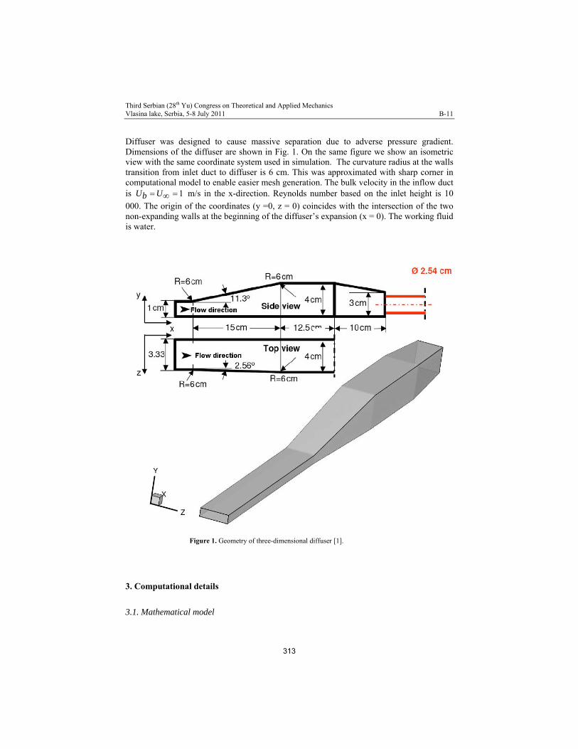
Diffuser was designed to cause massive separation due to adverse pressure gradient. Dimensions of the diffuser are shown in Fig. 1. On the same figure we show an isometric view with the same coordinate system used in simulation. The curvature radius at the walls transition from inlet duct to diffuser is 6 cm. This was approximated with sharp corner in computational model to enable easier mesh generation. The bulk velocity in the inflow duct is 1U Ub m/s in the x-direction. Reynolds number based on the inlet height is 10
000. The origin of the coordinates (y =0, z = 0) coincides with the intersection of the two non-expanding walls at the beginning of the diffuser’s expansion (x = 0). The working fluid is water.
Figure 1. Geometry of three-dimensional diffuser [1].
3. Computational details
3.1. Mathematical model
313
Third Serbian (28th Yu) Congress on Theoretical and Applied Mechanics Vlasina lake, Serbia, 5-8 July 2011 B-11
Reynolds-Averaged Navier-Stokes (RANS) system of equations is used to describe incompressible turbulent fluid flow in three dimensional diffuser:
0,i
i
U
x
(1)
1i j ji it
j i j j i
U U UU UP
t x x x x x
. (2)
Over-bar ( ) denotes time-averaged values, i.e. iU represents time-averaged velocity field.
Here, represents molecular viscosity, t represents turbulent viscosity. Turbulent
models based on Boussinesq hypothesis, or eddy viscosity models (EVM) imply determination of turbulent viscosity which takes part in linear relationship between Reynolds stress tensor (resulting after substituting the sum of average and fluctuating velocity fields into the Navier-Stokes equations) and averaged velocity gradients. Two-equation EVM reflect the idea that the information required for modeling the effect of turbulence on the mean flow are two independent scales, obtained from two independent transport equations [7]. All established two equations models use exact equation for the turbulent kinetic energy k , as a starting point. For the second, scale determining equation
there were many propositions, most notable ones were ( 3 2k L , where L is integral
length scale of turbulence), and ( 1 2 ~ 1k L T ) equations. These were modeled in
analogy with k using dimensional and intuitive arguments, which is the main reason for shortcomings of these equations. RANS turbulence models are known to be highly dissipative, which means they will not likely be triggered into the unsteady mode unless the flow instabilities are strong enough. The idea of SAS-SST model developed by Menter et al. [7] is to add the additional production term in the equation, which will be sensitive to unsteady fluctuations. In the chain of events, the term is increased; both turbulence kinetic energy k and turbulent viscosity t are reduced. Note, more the turbulent viscosity is being reduced more of the
flow unsteadiness is being resolved. Zero turbulent viscosity would mean there is no modeled part, there is just resolved one, as in the case of Direct Numerical Simulation (DNS). This promotes switching of momentum equations from steady to unsteady mode. The essence of SAS approach would be the ability to resolve turbulent structures, without dissipating them as classical RANS models do. The SAS concept is based on the introduction of the von Karman length-scale vkL into the
turbulence scale equation. The information provided by the von Karman length-scale allows SAS models to dynamically adjust to resolved scales in unsteady RANS simulation. This results in a LES like behavior in unsteady regions and standard RANS capabilities in stable flow regions. The transport equations for the SAS-SST model are [7], [8]:
i tk
i j k j
U kk kG c k
t x x x
(3)
314
Third Serbian (28th Yu) Congress on Theoretical and Applied Mechanics Vlasina lake, Serbia, 5-8 July 2011 B-11
21
,2
2 1(1 )i t
k SASi j j j j
U kG Q F
t x k x x x x
(4)
2
22 2 2
2 1 1max max , ,0SAS
vk j j j j
L k k kQ S C
L x x x xk
(5)
Where SASQ is the additional source term. Here L is the length scale of modeled
turbulence given by:
1 4L k c (6)
The von Karman length scale is given by:
''vk
SL
U
(7)
Scalar invariant of the strain rate tensor participates in the definition of von Karman length scale and also directly in SASQ term and is given here:
1
2 ;2
jiij ij ij
j i
UUS S S S
x x
(8)
Implementation of this model involves calculation of the second velocity derivative. It is generalized to three dimensions using the magnitude of the velocity Laplacian:
22
'' ii
j j
UU
x x
(9)
The model coefficients are: 2 3.51; 2 3; 2; 0.41C .
3.2. Numerical method Equations presented in the previous sub-section are solved by Finite-Volume method using ANSYS Fluent [8]. Convective terms are discretized using second order upwind scheme. Pressure based, sequential solver is used, and pressure-velocity coupling is realized through SIMPLE algorithm. Finest grid consisting of around one and a half million cells (1 578 720 cells precisely) ensured grid independent solution.
315

Third Serbian (28th Yu) Congress on Theoretical and Applied Mechanics Vlasina lake, Serbia, 5-8 July 2011 B-11
4. Results and discussion Precursor simulation in a rectangular duct was conducted first to generate inflow conditions for the simulation. The choice of the duct length compared to it’s height h was dependent on a need to have fully developed turbulence at the simulation domain inlet and had different values in other studies [3], [4]. In DNS study [6] the inflow development duct of 63h was used, and it included calculation of transition of initially laminar flow. Nothing similar was needed in our approach, therefore a duct with length equal to twenty times the diffuser inlet height was used.
Figure 2. Surface of constant x-velocity ( 0)xV , colored by turbulent viscosity [m2/s].
The wall boundary layer resolution with y being 1O in the finest grid was in the
domain of viscous sub-layer. Surface of constant zero stream-wise velocity colored by turbulent viscosity is shown in Fig. 2. This surface represents the delimiting region of the recirculation zone within the flow-filed. This figure presents first impression of flow topology.
316
Third Serbian (28th Yu) Congress on Theoretical and Applied Mechanics Vlasina lake, Serbia, 5-8 July 2011 B-11
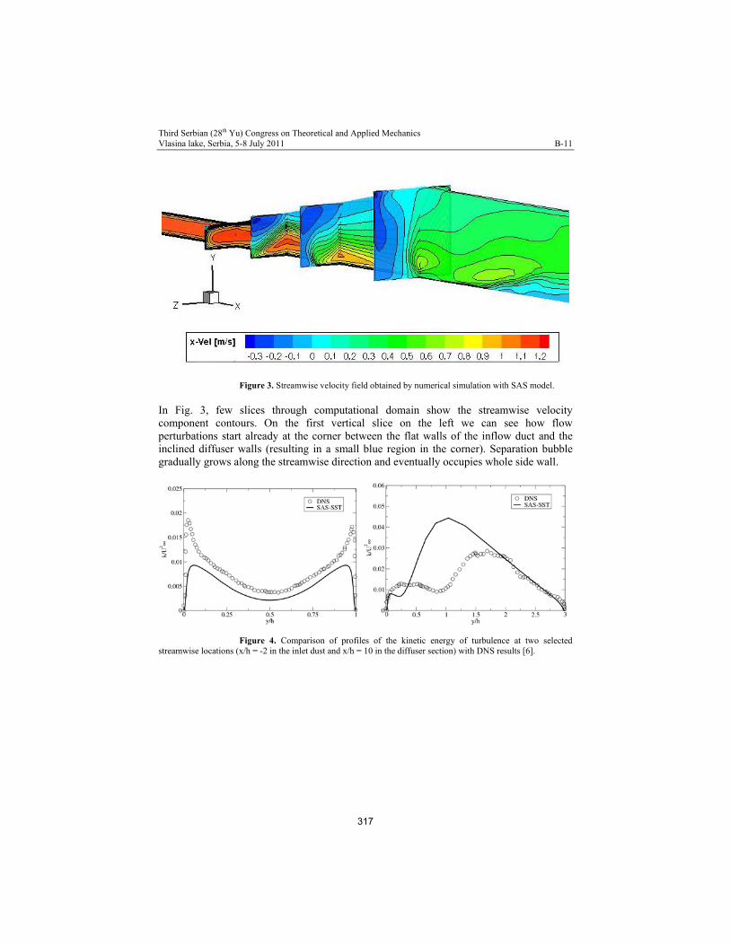
Figure 3. Streamwise velocity field obtained by numerical simulation with SAS model.
In Fig. 3, few slices through computational domain show the streamwise velocity component contours. On the first vertical slice on the left we can see how flow perturbations start already at the corner between the flat walls of the inflow duct and the inclined diffuser walls (resulting in a small blue region in the corner). Separation bubble gradually grows along the streamwise direction and eventually occupies whole side wall.
Figure 4. Comparison of profiles of the kinetic energy of turbulence at two selected streamwise locations (x/h = -2 in the inlet dust and x/h = 10 in the diffuser section) with DNS results [6].
317
Third Serbian (28th Yu) Congress on Theoretical and Applied Mechanics Vlasina lake, Serbia, 5-8 July 2011 B-11
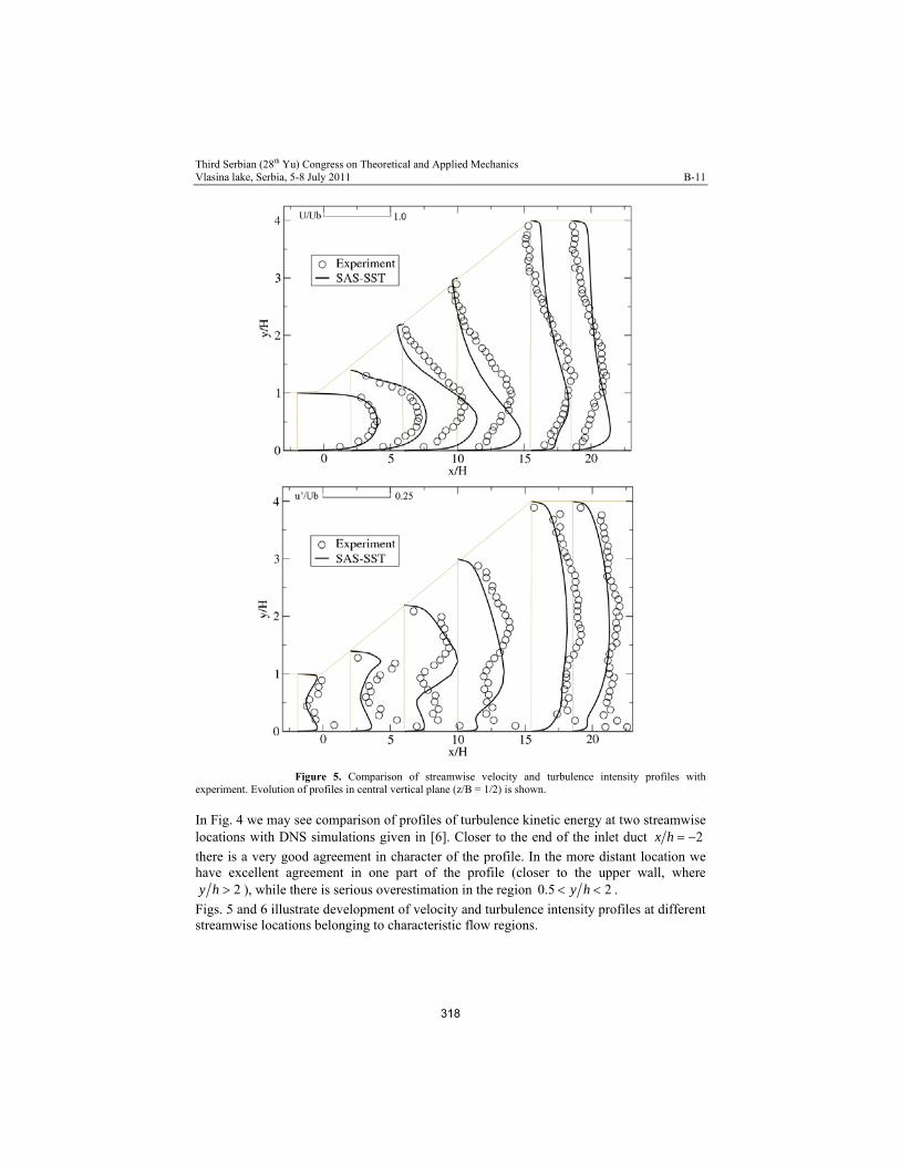
Figure 5. Comparison of streamwise velocity and turbulence intensity profiles with experiment. Evolution of profiles in central vertical plane (z/B = 1/2) is shown.
In Fig. 4 we may see comparison of profiles of turbulence kinetic energy at two streamwise locations with DNS simulations given in [6]. Closer to the end of the inlet duct 2x h
there is a very good agreement in character of the profile. In the more distant location we have excellent agreement in one part of the profile (closer to the upper wall, where
2y h ), while there is serious overestimation in the region 0.5 2y h .
Figs. 5 and 6 illustrate development of velocity and turbulence intensity profiles at different streamwise locations belonging to characteristic flow regions.
318
Third Serbian (28th Yu) Congress on Theoretical and Applied Mechanics Vlasina lake, Serbia, 5-8 July 2011 B-11
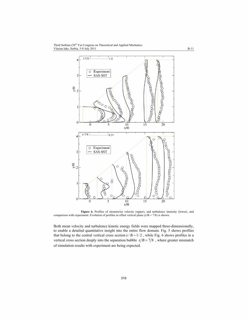
Figure 6. Profiles of streamwise velocity (upper), and turbulence intensity (lower), and comparison with experiment. Evolution of profiles in offset vertical plane (z/B = 7/8) is shown.
Both mean velocity and turbulence kinetic energy fields were mapped three-dimensionally, to enable a detailed quantitative insight into the entire flow domain. Fig. 5 shows profiles that belong to the central vertical cross section / 1/ 2z B , while Fig. 6 shows profiles in a vertical cross section deeply into the separation bubble 7 8z B , where greater mismatch
of simulation results with experiment are being expected.
319

Third Serbian (28th Yu) Congress on Theoretical and Applied Mechanics Vlasina lake, Serbia, 5-8 July 2011 B-11
5. Conclusions Scale Adaptive Simulation approach was used to predict flow in a three-dimensional diffuser, subject of a recent experiment [1], and of Direct Numerical Simulation study [6]. The flow configuration was chosen to exhibit three-dimensional recirculation pattern, adequate as a suitable benchmark for complex separated flow prediction by state of the art turbulence models. The aim our study was assessment of the SAS-SST model’s predictive performance. In our calculations grid resolution around one and a half million cells was adopted for critical assessment of model performance. Comparing with results from [3] and [4] we conclude that nothing less than hybrid LES/RANS approach with collecting statistics over large enough number of time steps to enable convergence of statistics will not enough for accurate prediction of separation region. This suggests that in the near future with further development of hybrid models we should expect more frequent dispatch from RANS models in engineering applications when complex, wall bounded flows are concerned.
Acknowledgement. The authors wish to express the gratitude to Ministry of Science of Republic of Serbia, for supporting their current research through projects TR-33036 and TR-35006.
References
[1] Cherry E M, Elkins C J, and Eaton J K (2007) Geometric Sensitivity of 3-D Separated Flows, Proc. of 5th International Symposium on Turbulence and Shear Flow Phenomena – TSFP5 Munich
[2] Jakirlić S, et. al. (2009) Report on 14th ERCOFTAC Workshop on Refined Turbulence Modeling. ERCOFTAC Bulletin No. 84.
[3] Abe K, Ohtsuka T (2010) An Investigation of LES and hybrid RANS/LES models for predicting 3D diffuser flow, Int. J. Heat and Fluid Flow, 31, pp. 833-844.
[4] Jakirlić S, et. al. (2010) Numerical and Physical Aspects in LES and hybrid RANS/LES of turbulent flow separation in a 3-D diffuser, Int. J. Heat and Fluid Flow, 31 pp. 820-832.
[5] Cherry E M, Iaccarino G, Elkins C J and Eaton J K (2006) Separated flow in a three-dimensional diffuser: preliminary validation, Center for Turbulence Research, Stanford University, Annual Research Brief pp. 31-40.
[6] Ohlsson J, Schlatter P, Fischer P F, Henningson D S (2009) DNS of separated flow in in a three-dimensional diffuser by the spectral element method. J. Fluid Mech. 650, pp. 307-318.
[7] Menter F R, Egorov Y (2010) The Scale-Adaptive Simulation Method for Unsteady Turbulent Flow Predictions. Part 1: Theory and Model Description, Flow Turbulence Combust, 85, pp. 113-138
[8] ANSYS Fluent Release 13.0 – Documentation, ANSYS, Inc., Canonsburg, 2010.
320
Third Serbian (28th Yu) Congress on Theoretical and Applied Mechanics Vlasina lake, Serbia, 5-8 July 2011 B-12
INVESTIGATION OF FULLY DEVELOPED PLANE TURBULENT CHANNEL FLOW BY MEANS OF REYNOLDS STRESS MODELS
B. Stanković , S. Belošević , M. Sijerčić , N. Crnomarković , V. Beljanski, I. Tomanović, A. Stojanović Institute of Nuclear Sciences Vinča, University of Belgrade, Laboratory of Thermal Engineering and Energy P.O. Box 522, 11001 Belgrade, Serbia, Tel. +381-11 3408-204 e-mail: [email protected]
Abstract. Two-dimensional fully developed turbulent plane-channel flow has served as canonical flow for studying near-wall turbulence and testing and calibration of Reynolds stress models. Most of the commonly used second-moment closure models were derived on the basis of the equilibrium Reynolds stress anisotropies in homogeneous shear flow. However, the behaviour of turbulent flows in the near-wall flow region is always highly inhomogeneous and therefore a modelling of wall-effects is required. The performance of the models in the inhomogeneous elementary or complex flows is not well known. Despite some opposing views in literature, in the present study, in order to compensate for difference in anisotropy of the Reynolds stress tensor in homogeneous and wall flows, a wall reflection term with the use of wall distance and unit normal vector is added to the pressure-strain model to provide good predictions for the log-layer of fully developed turbulent channel flow. In this paper the main characteristics of the mean flow and turbulent fields are numerically calculated by the second-moment closure models and compared against available experimental data. Available results from the direct numerical simulation are used to further clarify the behaviour of the proposed Reynolds stress models. Numerical results presented in this work provide verification of two-dimensional flow Reynolds stress models that are to be used in further numerical investigations of fully developed three-dimensional channel flows. Keywords: plane channel flow, Reynolds stress models, wall reflection term
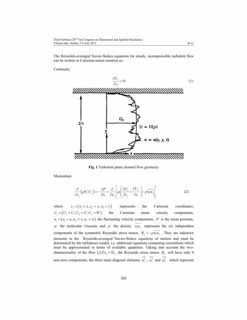
1. Introduction The fully developed turbulent plane channel flow, as one of the basic wall-bounded shear flows, has been extensively studied from the analytical, experimental and numerical point of view due to its simple geometry and fundamental nature of this flow case [1-5]. From the theoretical viewpoint, turbulent flow of an incompressible fluid with constant physical properties between two parallel plates separated at a distance 2h is considered. The plates are assumed infinitely wide. They are at rest with respect to the coordinate system used. The sketch of the flow is given in Figure 1. Since the flow is two-dimensional, the mean flow is assumed to be in the x y plane
0W and all derivatives of mean quantities on the z coordinate direction are assumed
to be zero 0z . The flow is steady 0t .
321
Third Serbian (28th Yu) Congress on Theoretical and Applied Mechanics Vlasina lake, Serbia, 5-8 July 2011 B-12
The Reynolds-averaged Navier-Stokes equations for steady, incompressible turbulent flow can be written in Cartesian tensor notation as: Continuity
0i
i
U
x
(1)
Fig. 1 Turbulent plane channel flow geometry
Momentum
jii j i j
j i j j i
UUPU U u u
x x x x x
(2)
where 1 2 3, ,ix x x x y x z represents the Cartesian coordinates,
1 2 3, ,iU U U U V U W the Cartesian mean velocity components,
1 2 3, ,iu u u u v u w the fluctuating velocity components, P is the mean pressure,
the molecular viscosity and the density. i ju u represents the six independent
components of the symmetric Reynolds stress tensor, ij i jR u u . They are unknown
elements in the Reynolds-averaged Navier-Stokes equations of motion and must be determined by the turbulence model, i.e. additional equations containing correlations which must be approximated in terms of available quantities. Taking into account the two-dimensionality of the flow 3 0x , the Reynolds stress tensor ijR will have only 4
non-zero components; the three main diagonal elements 21u , 2
2u and 23u which represent
322
Third Serbian (28th Yu) Congress on Theoretical and Applied Mechanics Vlasina lake, Serbia, 5-8 July 2011 B-12
the turbulent normal stresses, and one off-diagonal element 1 2u u which represents the
turbulent shear stress.
2. Reynolds stress models
2.1 Transport equation for i ju u . Turbulence closure problem and models.
The system of equations (1) and (2) is not closed, as i ju u is a new variable (second order
tensor) which emerges as a consequence of the averaging. The task of the RANS (Reynolds averaged Navier Stokes) modelling is to provide the approximated value (the model) of
i ju u in order to close and solve the system of equations (1) and (2). Differential second-
moment (Reynolds-stress models) turbulence closure models are regarded today as the best compromise between the current knowledge of the turbulence physics and possibilities of efficient solving of the modelled equations by means of the currently available computers. The foundation for a full Reynolds stress turbulence closure was laid by Rotta (1951) [6]. This new approach was based on the Reynolds stress transport equation [7], ie. balance equations for the Reynolds stresses, which can be written for high Reynolds number turbulent flow in Cartesian tensor notation as:
i jk ij ij ij ij
k
u uU P d
x
(3)
where ijP is the production, ijd is the diffusion, ij is the pressure-strain correlation, and
ij is the dissipation rate. In order to close the set of differential equations (1), (2) and (3),
the turbulence quantities on the right-hand side of (3) must be represented in terms of the mean velocities, Reynolds stresses and their derivatives (i.e. some of them need to be modelled).
The production term can be treated exactly, j iij i k j k
k k
U UP u u u u
x x
, and need not to be
modelled. At high Reynolds numbers the correlation 2 i jij
k k
u u
x x
- which is associated
with smallest eddies - is assumed to be locally isotropic. A common way to model the viscous destruction of stresses for high Re-number flows, as proposed by Rotta (1951), is:
2
3ij ij (4)
where 2
i ku x is the dissipation rate of the turbulent kinetic energy k and ij is
the Kronecker unit tensor.
323
Third Serbian (28th Yu) Congress on Theoretical and Applied Mechanics Vlasina lake, Serbia, 5-8 July 2011 B-12
2.2 Turbulent diffusion term The diffusive transport term consists of 3 parts: t p
ij ij ij ijd d d d . The molecular diffusion
ijd can be treated exactly and at high turbulence Re numbers is negligible. The remaining
two parts, the turbulent diffusion by fluctuating velocity and fluctuating pressure, tijd and
pijd , need to be modelled. ijd has a character of divergence, so that 0ij
V
d dV over a
closed domain bounded by impermeable surface (as follows from Gauss transformation of the volume integral into a surface integral). Hence the ijd term is of a transport (diffusive)
nature. The most popular way for modelling tijd is based on the generalized gradient
diffusion hypothesis (GGDH): k k ll
u C u ux
, where k is the time scale. Thus,
if is the Reynolds stress i ju u , the application of GGDH to the turbulent velocity
diffusion of Reynolds stresses yields:
i jtij i j k s k l
k k l
u ukd u u u C u u
x x x
(5)
known also as Daly-Harlow (1970) turbulent diffusion model , which is used in this paper. The turbulent transport by pressure fluctuations has a different nature (transport by the propagation of disturbances) and none of the gradient transport forms is applicable to modelling p
ijd . It is common to “lump” pijd with t
ijd and to adjust the coefficient sC
0.22sC . In many flows, except in flows driven by thermal buoyancy, the pressure
transport is smaller than the velocity transport, so that this approximation is appropriate.
2.3 Pressure-strain interaction – the slow and rapid terms
The pressure-strain correlation is of decisive importance for determination of the Reynolds stresses from their transport equations. Pressure fluctuations redistribute the turbulent stress among components to make turbulence more isotropic. Pressure-shear correlation takes care of the exchange of turbulence energy between the velocity components of different directions in order to bring about an equal distribution of the fluctuation intensities in all directions. The most common approach is to split the pressure-strain term,
jiij
j i
uup
x x
, into the following parts:
,1 ,2 ,ij ij ij ij w (6)
324
Third Serbian (28th Yu) Congress on Theoretical and Applied Mechanics Vlasina lake, Serbia, 5-8 July 2011 B-12
,1ij , “the slow term”, involving just fluctuating quantities, represents return to isotropy of
non-isotropic turbulence. Based on the idea that the pressure fluctuations tend to diminish turbulence anisotropy, Rotta (1951) proposed a simple linear model by which ,1ij is
proportional to the stress anisotropy tensor 2
3i j
ij ij
u ua
k . The expression is known as a
linear Return-to-Isotropy model:
,1 1 1
2
3i j
ij ij ij
u uC a C
k
(7)
where 1 1.8C .
,2ij , “the rapid term”, arising from the presence of the mean rate of strain
1
2ji
ijj i
UUS
x x
, acts as “isotropization” of the process of stress production due to
ijS . The complete influence of the mean strain on the pressure-strain correlation may be
expressed in the following form, as proposed by [8]:
2 2 2,2
8 30 2 8 22 2
11 3 55 11 3ji
ij ij ij ij ijj i
UUC C CP P k D P
x x
(8)
where: , ,j i k k iij i k j k ij i k j k i j
k k j i j
U U U U UP u u u u D u u u u P u u
x x x x x
and 2 0.4C . This model is also known as LRR-QI (Launder-Reece-Rodi Quasi-Isotropic
model). Launder, Reece and Rodi (1975) showed how second-order closure models could be calibrated and applied to the solution of practical engineering flows. The truncated version of (8), including only the first group of terms on the right side of (8) is known as “Isotropization of Production” (IP) model:
,2
2
3ij ij ijP P
(9)
where 0.6 .
2.4 Modelling the wall-effects on ij
325
Third Serbian (28th Yu) Congress on Theoretical and Applied Mechanics Vlasina lake, Serbia, 5-8 July 2011 B-12
The third term on the right-hand side of (6), ,ij w , is the wall reflection term (the near-wall
effect). Solid walls, by pressure fluctuation reflection, “splat” neighbouring eddies, which leads to the higher stress anisotropy and damping the velocity fluctuations in the wall- normal direction. The majority of models were developed for homogeneous flows. The most imporatant reason for it is the simplicity of this kind of flows, especially when compared to the wall bounded flows, which are strongly non-homogeneous due to the presence of a solid wall. Developed and tuned for homogeneous flows, these models usually perform rather poor when applied to wall flows, especially if the model equations are to be solved up to the wall. Two approaches used currently for modelling wall bounded turbulent flows differ much both in requirements for the mathematical model and the numerical solver. The high-Re-number approach, with wall function (used in this work), where some empirical laws are used to bridge a thin viscous sublayer close to the wall, requires a mathematical model to represent turbulence only at high-Re-number (though in highly inhomogeneous conditions), so that a relatively coarse numerical mesh can be used. The low-Re-number approach [9], where the model equations are integrated up to the solid boundary with the exact boundary conditions, requires more sophisticated model which needs to describe behaviour of the turbulence quantities in the wall vicinity where a multitude of effects (viscosity, high inhomogeneity, wall blockage, etc.) impose additional requirements for model modification. The model needs to satisfy the two-componentality limit which the turbulence obeys close to the wall due to a higher damping of the normal-to-the-wall fluctuatuions than of those in stream and spanwise directions. Therefore, a much finer numerical grid than for wall functions approach has to be used. Since developed with assumption of the local homogeneity and equilibrium, the models for homogeneous flows described above are not capable of representnig properly the behaviour of turbulent flows which are far from the equilibrium, and particularly in the near-wall flow region which is always highly inhomogeneous. Therefore, in order to compensate for difference in anisotropy of the Reynolds stress tensor in homogeneous and wall flows [10] at comparable ratio of production/dissipation, a wall effect term, ,ij w , is added to model
for ij . The near-wall correction to the pressure-strain correlation, for the plane channel flow, was proposed by [8] in the following form:
3 2
,
2 1 10.125 0.015
3 2ij w i j ij ij ijw w
ku u k P D
k y h y
(10)
where 2h is the distance between two walls and wy is the distance from the wall.
In somewhat different manner, the wall reflection term is decomposed into a slow and a rapid contribution as done with the pressure-strain model: , ,1 ,2
w wij w ij ij , as proposed
in [11]:
326
Third Serbian (28th Yu) Congress on Theoretical and Applied Mechanics Vlasina lake, Serbia, 5-8 July 2011 B-12
,1 1
,2 2 ,2 ,2 ,2
3 3
2 2
3 3
2 2
w wij k m k m ij i k k j k j k i w
w wij km k m ij ik k j jk k i w
C u u n n u u n n u u n n fk
C n n n n n n f
(11)
where 1 2 3, ,n n n n
is the unit vector normal to the wall and wf is a function which
indicates proximity of a wall. The most frequently used definition of wf was proposed by
[8] :
1
wl w
lf
C y (12)
where 3 4 2.5lC C is a coefficient chosen to provide unity value of wf in the log-law
region, 3 2k
l
is the turbulent length scale and wy is the distance from the nearest wall.
For the case of plane channel flow instead of 1
wy the expression
1 1
2w wy h y
should be
used. Function wf has value of unity close to a wall and diminishes as the distance to the
wall increases. The model coefficients proposed by [11] are: 1 0.5wC and 2 0.3wC (used
in model denoted as GL-a). However, in this paper, according to Obi (1991), the value of
2 0.18wC (used in model denoted as GL-b) is tested and the obtained results are
compared. The model GL-b showed slightly better performance in comparison with the model GL-a. 2.5 The model equation for
The exact equation for gives some indication of the meanings and importance of various terms. In the differential second-moment turbulence closure models the same basic form of model equation for is used as in the k model. Hence, the model equation for has the form:
2
1 2i k i
k k lk k l k
u u UkU C u u C C
t x x x k x k
(13)
where the coefficients 1C and 2C have the same values as in the k model, 1 1.45C and 2 1.92C , except for the new coefficient 0.18C .
In this paper three different Reynolds stress models (denoted as LRR1, LRR2 and GL) are numerically tested, according to the modelling equations (8)-(11) of the rapid pressure-
327
Third Serbian (28th Yu) Congress on Theoretical and Applied Mechanics Vlasina lake, Serbia, 5-8 July 2011 B-12
strain term and wall reflection term, Table 1. The remaining modelling equations of the other terms for these models are the same (Eq. (4), (5), (7) and (13)).
Rapid and wall-echo terms
LRR1 LRR2 GL
,2ij Eq. (8) Eq. (9) Eq. (9)
,ij w Eq. (10) Eq. (10) Eq. (11)
Table 1. LRR1, LRR2 and GL second-moment closure models - ,2ij and ,ij w terms
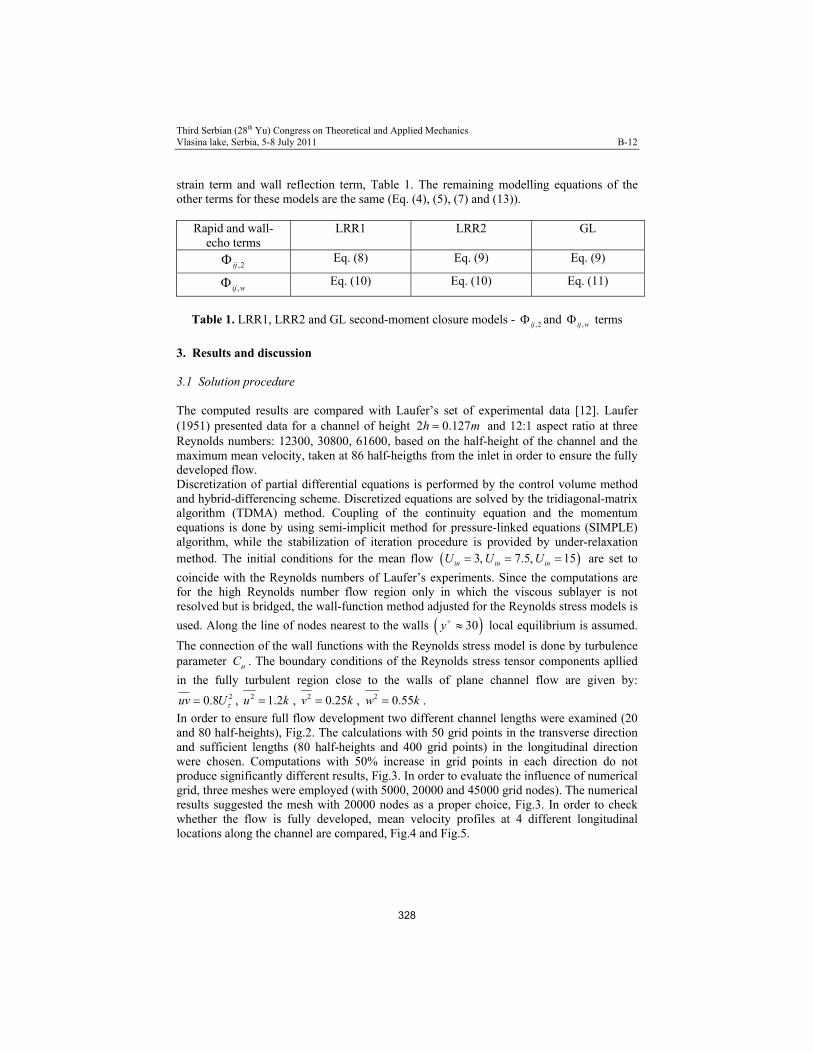
3. Results and discussion 3.1 Solution procedure The computed results are compared with Laufer’s set of experimental data [12]. Laufer (1951) presented data for a channel of height 2 0.127h m and 12:1 aspect ratio at three Reynolds numbers: 12300, 30800, 61600, based on the half-height of the channel and the maximum mean velocity, taken at 86 half-heigths from the inlet in order to ensure the fully developed flow. Discretization of partial differential equations is performed by the control volume method and hybrid-differencing scheme. Discretized equations are solved by the tridiagonal-matrix algorithm (TDMA) method. Coupling of the continuity equation and the momentum equations is done by using semi-implicit method for pressure-linked equations (SIMPLE) algorithm, while the stabilization of iteration procedure is provided by under-relaxation method. The initial conditions for the mean flow 3, 7.5, 15in in inU U U are set to
coincide with the Reynolds numbers of Laufer’s experiments. Since the computations are for the high Reynolds number flow region only in which the viscous sublayer is not resolved but is bridged, the wall-function method adjusted for the Reynolds stress models is
used. Along the line of nodes nearest to the walls 30y local equilibrium is assumed.
The connection of the wall functions with the Reynolds stress model is done by turbulence parameter C . The boundary conditions of the Reynolds stress tensor components apllied
in the fully turbulent region close to the walls of plane channel flow are given by: 20.8uv U , 2 1.2u k , 2 0.25v k , 2 0.55w k .
In order to ensure full flow development two different channel lengths were examined (20 and 80 half-heights), Fig.2. The calculations with 50 grid points in the transverse direction and sufficient lengths (80 half-heights and 400 grid points) in the longitudinal direction were chosen. Computations with 50% increase in grid points in each direction do not produce significantly different results, Fig.3. In order to evaluate the influence of numerical grid, three meshes were employed (with 5000, 20000 and 45000 grid nodes). The numerical results suggested the mesh with 20000 nodes as a proper choice, Fig.3. In order to check whether the flow is fully developed, mean velocity profiles at 4 different longitudinal locations along the channel are compared, Fig.4 and Fig.5.
328
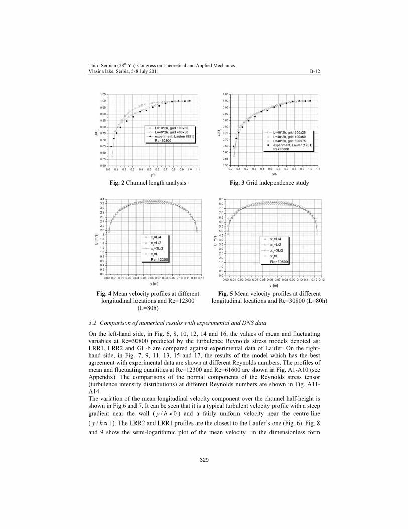
Third Serbian (28th Yu) Congress on Theoretical and Applied Mechanics Vlasina lake, Serbia, 5-8 July 2011 B-12
Fig. 2 Channel length analysis Fig. 3 Grid independence study
Fig. 4 Mean velocity profiles at different longitudinal locations and Re=12300
(L=80h)
Fig. 5 Mean velocity profiles at different longitudinal locations and Re=30800 (L=80h)
3.2 Comparison of numerical results with experimental and DNS data
On the left-hand side, in Fig. 6, 8, 10, 12, 14 and 16, the values of mean and fluctuating variables at Re=30800 predicted by the turbulence Reynolds stress models denoted as: LRR1, LRR2 and GL-b are compared against experimental data of Laufer. On the right-hand side, in Fig. 7, 9, 11, 13, 15 and 17, the results of the model which has the best agreement with experimental data are shown at different Reynolds numbers. The profiles of mean and fluctuating quantities at Re=12300 and Re=61600 are shown in Fig. A1-A10 (see Appendix). The comparisons of the normal components of the Reynolds stress tensor (turbulence intensity distributions) at different Reynolds numbers are shown in Fig. A11-A14. The variation of the mean longitudinal velocity component over the channel half-height is shown in Fig.6 and 7. It can be seen that it is a typical turbulent velocity profile with a steep gradient near the wall ( / 0y h ) and a fairly uniform velocity near the centre-line
( / 1y h ). The LRR2 and LRR1 profiles are the closest to the Laufer’s one (Fig. 6). Fig. 8
and 9 show the semi-logarithmic plot of the mean velocity in the dimensionless form
329
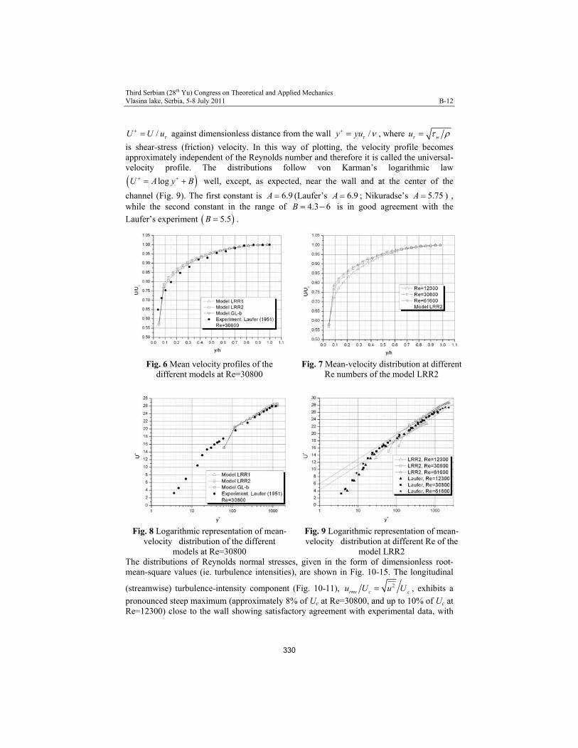
Third Serbian (28th Yu) Congress on Theoretical and Applied Mechanics Vlasina lake, Serbia, 5-8 July 2011 B-12
/U U u against dimensionless distance from the wall /y yu , where wu
is shear-stress (friction) velocity. In this way of plotting, the velocity profile becomes approximately independent of the Reynolds number and therefore it is called the universal-velocity profile. The distributions follow von Karman’s logarithmic law
logU A y B well, except, as expected, near the wall and at the center of the
channel (Fig. 9). The first constant is 6.9A (Laufer’s 6.9A ; Nikuradse’s 5.75A ) , while the second constant in the range of 4.3 6B is in good agreement with the
Laufer’s experiment 5.5B .
Fig. 6 Mean velocity profiles of the
different models at Re=30800 Fig. 7 Mean-velocity distribution at different
Re numbers of the model LRR2
Fig. 8 Logarithmic representation of mean-velocity distribution of the different
models at Re=30800
Fig. 9 Logarithmic representation of mean-velocity distribution at different Re of the
model LRR2 The distributions of Reynolds normal stresses, given in the form of dimensionless root-mean-square values (ie. turbulence intensities), are shown in Fig. 10-15. The longitudinal
(streamwise) turbulence-intensity component (Fig. 10-11), 2rms c cu U u U , exhibits a
pronounced steep maximum (approximately 8% of Uc at Re=30800, and up to 10% of Uc at Re=12300) close to the wall showing satisfactory agreement with experimental data, with
330
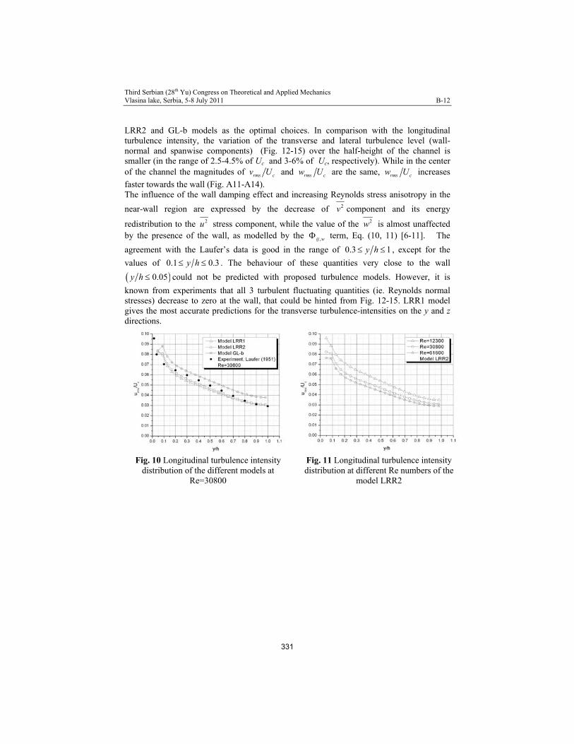
Third Serbian (28th Yu) Congress on Theoretical and Applied Mechanics Vlasina lake, Serbia, 5-8 July 2011 B-12
LRR2 and GL-b models as the optimal choices. In comparison with the longitudinal turbulence intensity, the variation of the transverse and lateral turbulence level (wall-normal and spanwise components) (Fig. 12-15) over the half-height of the channel is smaller (in the range of 2.5-4.5% of Uc and 3-6% of Uc, respectively). While in the center of the channel the magnitudes of rms cv U and rms cw U are the same, rms cw U increases
faster towards the wall (Fig. A11-A14). The influence of the wall damping effect and increasing Reynolds stress anisotropy in the
near-wall region are expressed by the decrease of 2v component and its energy
redistribution to the 2u stress component, while the value of the 2w is almost unaffected by the presence of the wall, as modelled by the ,ij w term, Eq. (10, 11) [6-11]. The
agreement with the Laufer’s data is good in the range of 0.3 1y h , except for the
values of 0.1 0.3y h . The behaviour of these quantities very close to the wall
0.05y h could not be predicted with proposed turbulence models. However, it is
known from experiments that all 3 turbulent fluctuating quantities (ie. Reynolds normal stresses) decrease to zero at the wall, that could be hinted from Fig. 12-15. LRR1 model gives the most accurate predictions for the transverse turbulence-intensities on the y and z directions.
Fig. 10 Longitudinal turbulence intensity distribution of the different models at
Re=30800
Fig. 11 Longitudinal turbulence intensity distribution at different Re numbers of the
model LRR2
331
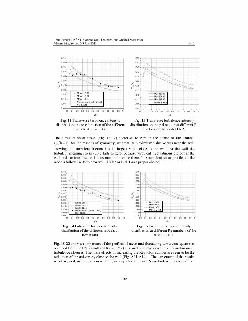
Third Serbian (28th Yu) Congress on Theoretical and Applied Mechanics Vlasina lake, Serbia, 5-8 July 2011 B-12
Fig. 12 Transverse turbulence intensity distribution on the y direction of the different
models at Re=30800
Fig. 13 Transverse turbulence intensity distribution on the y direction at different Re
numbers of the model LRR1 The turbulent shear stress (Fig. 16-17) decreases to zero in the centre of the channel
1y h for the reasons of symmetry, whereas its maximium value occurs near the wall
showing that turbulent friction has its largest value close to the wall. At the wall the turbulent shearing stress curve falls to zero, because turbulent fluctuatuions die out at the wall and laminar friction has its maximum value there. The turbulent shear profiles of the models follow Laufer’s data well (LRR2 or LRR1 as a proper choice).
Fig. 14 Lateral turbulence intensity
distribution of the different models at Re=30800
Fig. 15 Lateral turbulence intensity distribution at different Re numbers of the
model LRR1 Fig. 18-22 show a comparison of the profiles of mean and fluctuating turbulence quantities obtained from the DNS results of Kim (1987) [13] and predictions with the second-moment turbulence closures. The main effects of increasing the Reynolds number are seen to be the reduction of the anisotropy close to the wall (Fig. A11-A14). The agreement of the results is not as good, in comparison with higher Reynolds numbers. Nevertheless, the results from
332
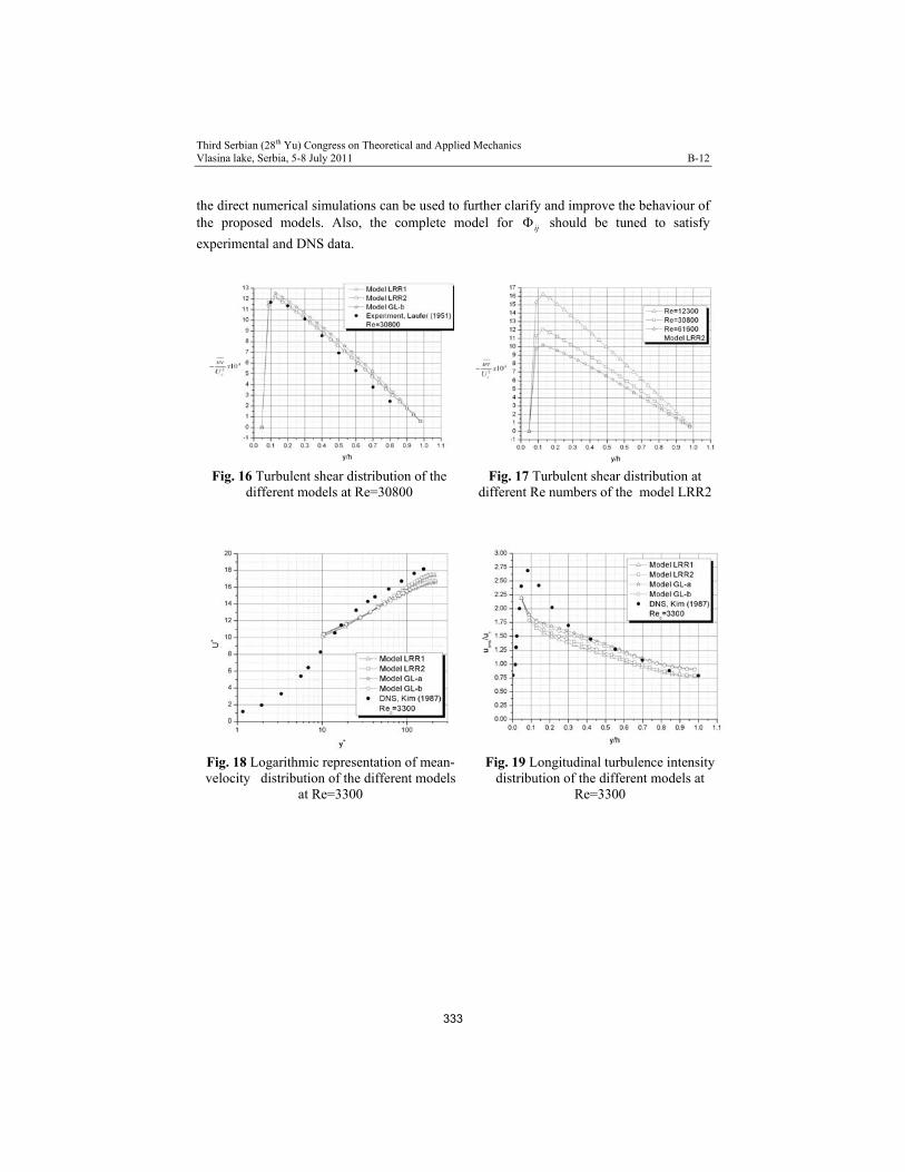
Third Serbian (28th Yu) Congress on Theoretical and Applied Mechanics Vlasina lake, Serbia, 5-8 July 2011 B-12
the direct numerical simulations can be used to further clarify and improve the behaviour of the proposed models. Also, the complete model for ij should be tuned to satisfy
experimental and DNS data.
Fig. 16 Turbulent shear distribution of the
different models at Re=30800 Fig. 17 Turbulent shear distribution at
different Re numbers of the model LRR2
Fig. 18 Logarithmic representation of mean-velocity distribution of the different models
at Re=3300
Fig. 19 Longitudinal turbulence intensity distribution of the different models at
Re=3300
333

Third Serbian (28th Yu) Congress on Theoretical and Applied Mechanics Vlasina lake, Serbia, 5-8 July 2011 B-12
Fig. 20 Transverse turbulence intensity
distribution on the y direction of the different models at Re=3300
Fig. 21 Lateral turbulence intensity distribution of the different models at
Re=3300
Fig. 22 Turbulent shear distribution of the different models at Re=3300
4. Conclusion
The test problem was the numerical investigation of fully-developed planne channel flow at high Reynolds numbers. Three Reynolds stress closure models are used in the computations. Among a large number of experimental studies Laufer's data was chosen as the best compromise for the results comparison. The main characteristics of the mean flow and turbulent fields are compared against experimental data. All three models produce similar predictions of the mean flow velocity, which agree well with the logarithmic law of the wall over most of the channel cross-section. LRR2 and GLb give the best prediction of the longitudinal Reynolds normal stress, whereas LRR1 gives the most accurate prediction of the transverse and lateral components of the normal Reynolds stresses. All models predict the shear stress distribution correctly. The significance of the turbulence Reynolds stress profiles, obtained in the analysed test-cases of fully developed two-dimensional
334
Third Serbian (28th Yu) Congress on Theoretical and Applied Mechanics Vlasina lake, Serbia, 5-8 July 2011 B-12
channel flow, is in the fact that these distribution laws can be used as an indicator for the check, analysis of the behaviour of the turbulent quantities and defining of the boundary conditions for other complex flows.
Acknowledgement. This work has been supported by the Republic of Serbia Ministry of Education and Science (project: “Increase in energy and ecology efficiency of processes in pulverized coal-fired furnace and optimization of utility steam boiler air preheater by using in-house developed software tools”, No. 33018). References 1. Zanoun E.S., Durst F., 2009, Turbulent momentum transport and kinetic energy
production in plane-channel flows, International Journal of Heat and Mass Transfer, vol. 52, pp. 4117-4124
2. Buschmann M., Gad-el-Hak M., 2010, Normal and cross-flow Reynolds stresses: differences between confined and semi-confined flows, Exp. Fluids, vol. 49, pp. 213-223
3. Gerolymos G.A., Sauret E., Vallet I., 2004, Contribution to single-point closure Reynolds-stress modeling of inhomogeneous flow, Theoret. Comput. Fluid Dynamics, vol. 17, pp. 407-431
4. Abe H., Kawamura H., 2001, Direct numerical simulation of a fully developed turbulent channel flow with respect to the Reynolds number dependence, Transactions of the ASME, Journal of Fluids Engineering, vol. 123, pp. 382-393
5. Demuren A.O., Sarkar S., 1993, Perspective: Systematic study of Reynolds stress closure models in the computations of plane channel flows, Transactions of the ASME, Journal of Fluids Engineering, vol. 115, pp. 5-12
6. Sijerčić M., 1998, Matematičko modeliranje kompleksnih turbulentnih transportnih procesa, Jugoslovensko društvo termičara i Institut za nuklearne nauke „Vinča“, Beograd
7. Hanjalić K., 1984, Modeliranje turbulentnih transportnih procesa, Zbornik radova, Knjiga 13, ANU BiH, Odeljenje tehničkih nauka, Sarajevo
8. Launder B.E., Reece G.J. and Rodi W., 1975, Progress in the development of a Reynolds-stress turbulence closure, Journal of Fluid Mechanics, vol. 68, pp. 537-566
9. Jakirlić S., 1991, Doprinos razvoju diferencijalnog naponskog modela turbulencije uvođenjem efekata viskoznosti i uticaja čvrstog zida, Magistarski rad, Univerzitet u Sarajevu, Mašinski fakultet - Sarajevo
10. Hadžić I., 1999, Second-Moment Closure Modelling of Transitional and Unsteady Turbulent Flows, PhD Thesis, Technical University Delft
11. Gibson M.M. and Launder B.E., 1978, Ground effects on pressure fluctuations in the atmospheric boundary layer, Journal of Fluid Mechanics, vol. 86, pp. 491-511
12. Laufer J., 1951, Investigation of turbulent flow in a two-dimensional channel, NACA Report 1053
13. Kim J., Moin P. and Moser R., 1987, Turbulence statistics in fully developed channel flow at low Reynolds number, Journal of Fluid Mechanics, vol. 177, pp. 133-166
335
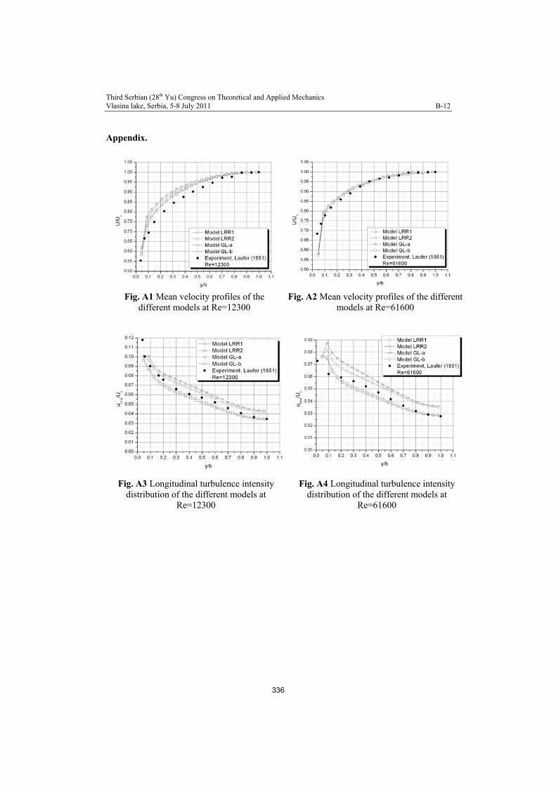
Third Serbian (28th Yu) Congress on Theoretical and Applied Mechanics Vlasina lake, Serbia, 5-8 July 2011 B-12
Appendix.
Fig. A1 Mean velocity profiles of the
different models at Re=12300 Fig. A2 Mean velocity profiles of the different
models at Re=61600
Fig. A3 Longitudinal turbulence intensity distribution of the different models at
Re=12300
Fig. A4 Longitudinal turbulence intensity distribution of the different models at
Re=61600
336
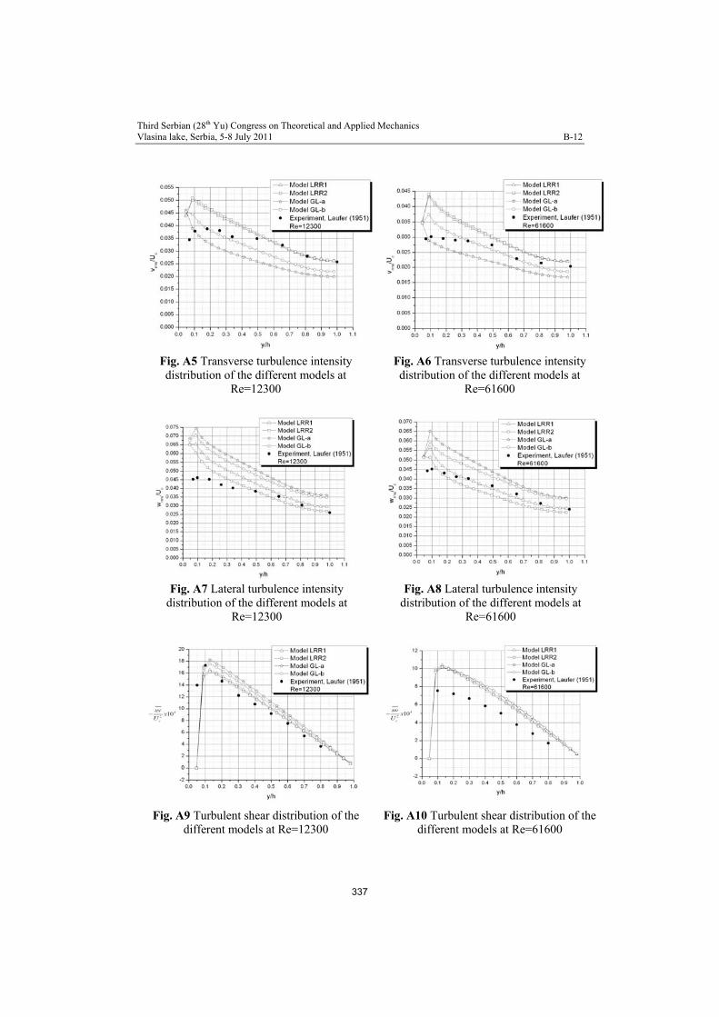
Third Serbian (28th Yu) Congress on Theoretical and Applied Mechanics Vlasina lake, Serbia, 5-8 July 2011 B-12
Fig. A5 Transverse turbulence intensity distribution of the different models at
Re=12300
Fig. A6 Transverse turbulence intensity distribution of the different models at
Re=61600
Fig. A7 Lateral turbulence intensity
distribution of the different models at Re=12300
Fig. A8 Lateral turbulence intensity distribution of the different models at
Re=61600
Fig. A9 Turbulent shear distribution of the different models at Re=12300
Fig. A10 Turbulent shear distribution of the different models at Re=61600
337
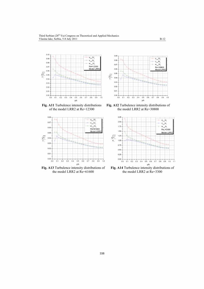
Third Serbian (28th Yu) Congress on Theoretical and Applied Mechanics Vlasina lake, Serbia, 5-8 July 2011 B-12
Fig. A11 Turbulence intensity distributions
of the model LRR2 at Re=12300 Fig. A12 Turbulence intensity distributions of
the model LRR2 at Re=30800
Fig. A13 Turbulence intensity distributions of
the model LRR2 at Re=61600 Fig. A14 Turbulence intensity distributions of
the model LRR2 at Re=3300
338