We study the mechanisms that are associated with the … · We study the mechanisms that are...

econstor www.econstor.eu

Der Open-Access-Publikationsserver der ZBW – Leibniz-Informationszentrum WirtschaftThe Open Access Publication Server of the ZBW – Leibniz Information Centre for Economics

Standard-Nutzungsbedingungen:

Die Dokumente auf EconStor dürfen zu eigenen wissenschaftlichenZwecken und zum Privatgebrauch gespeichert und kopiert werden.

Sie dürfen die Dokumente nicht für öffentliche oder kommerzielleZwecke vervielfältigen, öffentlich ausstellen, öffentlich zugänglichmachen, vertreiben oder anderweitig nutzen.

Sofern die Verfasser die Dokumente unter Open-Content-Lizenzen(insbesondere CC-Lizenzen) zur Verfügung gestellt haben sollten,gelten abweichend von diesen Nutzungsbedingungen die in der dortgenannten Lizenz gewährten Nutzungsrechte.

Terms of use:

Documents in EconStor may be saved and copied for yourpersonal and scholarly purposes.

You are not to copy documents for public or commercialpurposes, to exhibit the documents publicly, to make thempublicly available on the internet, or to distribute or otherwiseuse the documents in public.

If the documents have been made available under an OpenContent Licence (especially Creative Commons Licences), youmay exercise further usage rights as specified in the indicatedlicence.

zbw Leibniz-Informationszentrum WirtschaftLeibniz Information Centre for Economics

Riphahn, Regina T.; Schwientek, Caroline

Working Paper

What Drives the Reversal of the Gender EducationGap? Evidence from Germany

CESifo Working Paper, No. 5395

Provided in Cooperation with:Ifo Institute – Leibniz Institute for Economic Research at the University ofMunich

Suggested Citation: Riphahn, Regina T.; Schwientek, Caroline (2015) : What Drives theReversal of the Gender Education Gap? Evidence from Germany, CESifo Working Paper, No.5395

This Version is available at:http://hdl.handle.net/10419/113728

What Drives the Reversal of the Gender Education Gap? Evidence from Germany

Regina T. Riphahn Caroline Schwientek

CESIFO WORKING PAPER NO. 5395 CATEGORY 5: ECONOMICS OF EDUCATION

JUNE 2015

An electronic version of the paper may be downloaded • from the SSRN website: www.SSRN.com • from the RePEc website: www.RePEc.org

• from the CESifo website: Twww.CESifo-group.org/wp T

ISSN 2364-1428

http://www.ssrn.com/

http://www.repec.org/

http://www.cesifo-group.de/

CESifo Working Paper No. 5395

What Drives the Reversal of the Gender Education Gap? Evidence from Germany

Abstract We study the mechanisms that are associated with the gender education gap and its reversal in Germany. We focus on three outcomes, graduation from upper secondary school, any tertiary education, and tertiary degree. Neither individual and family background nor labor market characteristics appear to be strongly associated with the gender education gap. There is some evidence that the gender gap in upper secondary education reflects the rising share of single parent households which impacts boys’ attainment more than girls’. The gender education gap in tertiary education is correlated with the development of class sizes and social norms.

JEL-Code: I210, J160.

Keywords: educational attainment, wage premium, gender gap.

Regina T. Riphahn* University of Erlangen-Nürnberg

Lange Gasse 20 Germany – 90403 Nuremberg

[email protected]

Caroline Schwientek University of Erlangen-Nürnberg

Lange Gasse 20 Germany – 90403 Nuremberg

[email protected]

*corresponding author 1 June 2015 We gratefully acknowledge helpful referee comments and comments from the cesifo Economics of Education conference 2013.

1

1. Introduction

In many industrialized countries the gender education gap recently changed direction such that

the educational attainment of females now often exceeds that of males. In advanced economies

the gender difference in the share of 30-34 years olds with a tertiary degree shifted from 5.6

percentage points in favor of men in 1980 to 6.6 points in favor of women in 2005 (Parro 2012).

It is intriguing to explore the determinants of this development and it is important: the rising

female advantage in higher education may affect societies in many ways, among them, e.g.,

shifting labor market structures and family formation patterns.

We investigate the mechanisms behind the reversal of the gender education gap in

secondary and tertiary education in Germany. The German case is of special interest for various

reasons: being a federal state Germany offers the opportunity to study the role of educational

institutions that vary at the state level. At the same time, the education system itself has been

reasonably stable over time such that there are no independent reforms confounding the

development of educational choices (cf., Pekkarinen 2008). Also, a reversal of gender

differences is particularly remarkable in Germany where until today the male breadwinner

model dominates welfare state institutions and the income tax system.

So far, the international literature focuses on changing gender patterns in tertiary

education, only. Goldin et al. (2006) look at college completion rates in the U.S. and discuss

various mechanisms behind the relative progress of females: the rising expectation of

permanent labor force attachment encouraged higher investments in human capital particularly

for the female birth cohorts since 1960. For these birth cohorts contraceptives became available,

the age at first marriage increased, and rising divorce rates further incentivized female economic

independence. Some authors argue that women benefited from the shift in labor demand to

college educated workers and from a college wage premium that was higher for females than

2

for males (e.g., Charles and Luoh 2003, DiPrete and Buchmann 2006).1 Also, gender

differences in non-cognitive abilities are considered to render females' effort cost of higher

education lower than that of males.

Becker et al. (2010) study gender-specific changes in the costs and benefits of higher

education. The authors consider the female advantage in the total cost of education to be central

to the reversal of the gender education gap. In particular, higher non-cognitive skills of females,

a lower incidence of behavioral problems, and the smaller variance in the distribution of non-

cognitive skills render the female supply of college educated labor more elastic than that of

males. The authors argue that the rising demand for college educated workers generated a larger

supply response among females rather than males.

The literature on the gender education gap outside of the U.S. is slim. Christofides et al.

(2010) confirm much of the U.S. evidence for Canadian university attendance. They find that

the university wage premium explains most of the changes over time with smaller roles for

changes in tuition and real incomes.2

For the case of Germany only Legewie and DiPrete (2009) address the gender education

gap.3 They focus on the role of parental education and point out that in terms of college

completion U.S. females have overtaken U.S. males while German females only narrowed the

gap. The authors argue that in the U.S. − but not in Germany − a cultural transformation lifted

prior constraints on female tertiary education. We extend this study by considering a much

broader set of mechanisms potentially affecting the gender education gap and by including more

recent birth cohorts.

1 In contrast, Hubbard (2011) points out that the college wage premium for women does not exceed that of men, once unbiased estimations are used. 2 Further important contributions to this literature are, e.g., DiPrete and Buchmann (2006), Hubbard (2011), Bailey and Dynarski (2011), Parro (2012), and Cho (2007). 3 Beyond that the relevant German literature mainly comprises studies on the development of male and female returns to education over time; see, e.g., Ammermüller and Weber (2005), Schnabel and Schnabel (2002), Boockmann and Steiner (2006), Fitzenberger and Kohn (2006), or Gebel and Pfeiffer (2010).

3

We study determinants of the German gender education gap and its reversal for the birth

cohorts 1965 through 1989. In contrast to most of the literature we consider education outcomes

at different stages of the life cycle, i.e., secondary as well as tertiary education outcomes.4 We

describe recent developments and evaluate the relevance of potential determinants of the gender

education gap and its reversal including a rich set of indicators of wage and employment

premiums, shifts in occupation-specific skill requirements, characteristics of the education

system, and demographic developments.

Using individual level data we find that neither individual and family background nor

labor market characteristics appear to be strongly associated with the gender education gap.

Based on analyses of pooled data there is some evidence that the gender gap in upper secondary

education is associated with the rising share of single parent households which impacts boys'

attainment more than girls'. The gender education gap in tertiary education and its reversal are

correlated with the development of class sizes and social norms.

The next section sketches the German education system and section 3 surveys the

developments in secondary and tertiary educational attainment. Then we describe our data and

empirical approach. Our analysis and a detailed discussion of the considered mechanisms

follow in section 5. Next, we discuss robustness tests and section 7 concludes.

2. Institutional Background

We briefly summarize some key features of the German education system. Starting at

age three children can attend Kindergarten, which traditionally provides instruction for half a

day until midday. At about age six children enter elementary school, which generally lasts four

years. At age ten, pupils move on to secondary school which - generally - offers three tracks:

lower secondary school (Hauptschule) lasts another six years and prepares for vocational

4 For a related approach see Bertocchi and Bozzano (2014).

4

training in blue collar occupations and crafts. Intermediate secondary school

(Realschule/Mittelschule) also provides six years of instruction and typically prepares for

vocational training in white collar occupations. At upper secondary schools (Gymnasium) eight

or nine years of education lead to the upper secondary school degree (Abitur), which is required

for admission to tertiary education. In principle, an initial track choice can be reversed later on,

but this happens only rarely. Since the 1960s the "education expansion" yielded a steady

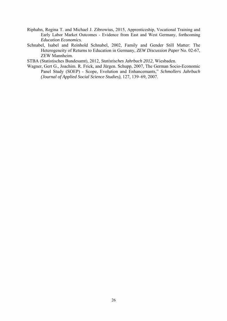
improvement in secondary education outcomes over subsequent birth cohorts (see Figure 1).5

Once pupils leave secondary school different pathways are available: those with an

upper secondary school degree can start tertiary education. Generally, however, a transition into

vocational training is most common and possible for graduates from all tracks. Instead of

pursuing tertiary education, vocational training, or military or substitute service, secondary

school graduates may work as unqualified workers, leave the labor force, or become

unemployed.6 As of 2011, about 67 percent of the German adult working age (age 25-65)

population held a degree from the vocational training system, mostly from an apprenticeship,

15 percent held a tertiary degree, and 17 percent held no vocational degree (STBA 2012).

The German education system is administered at the level of federal states. The states

regulate the transition from elementary to secondary school, educational curricula, the number

and size of secondary schools, teacher training and hiring, and budgets.7 Some states are more

restrictive than others in allowing access to upper secondary schools, however, most features

of the educational system such as curricula, teacher training, employment conditions, and

5 Jürges and Schneider (2011) discuss biases in track assignment that result from developmental differences by gender and relative age at the disadvantage of boys (Pekkarinen (2008) also shows evidence on this issue). However, as the German track system existed for many decades, a permanent gender bias can hardly explain recent changes in the gender education gap. 6 For details on the German vocational training system, see, e.g., Riphahn and Zibrowius (2015). 7 In contrast to the local property tax based funding of schools in the U.S., in there is no direct or formal connection between school budgets and local wealth in Germany as all schools are paid by the state government.

5

salaries are similar across states (KMK 2013). Also, the tertiary education system is similar

across states.

3. Development of the gender education gap

As in other countries, men in Germany traditionally received more education than

women (Parro 2012). Early in the twentieth century about 10 percent of male and five percent

of female birth cohorts graduated from upper secondary school (Riphahn 2011). These shares

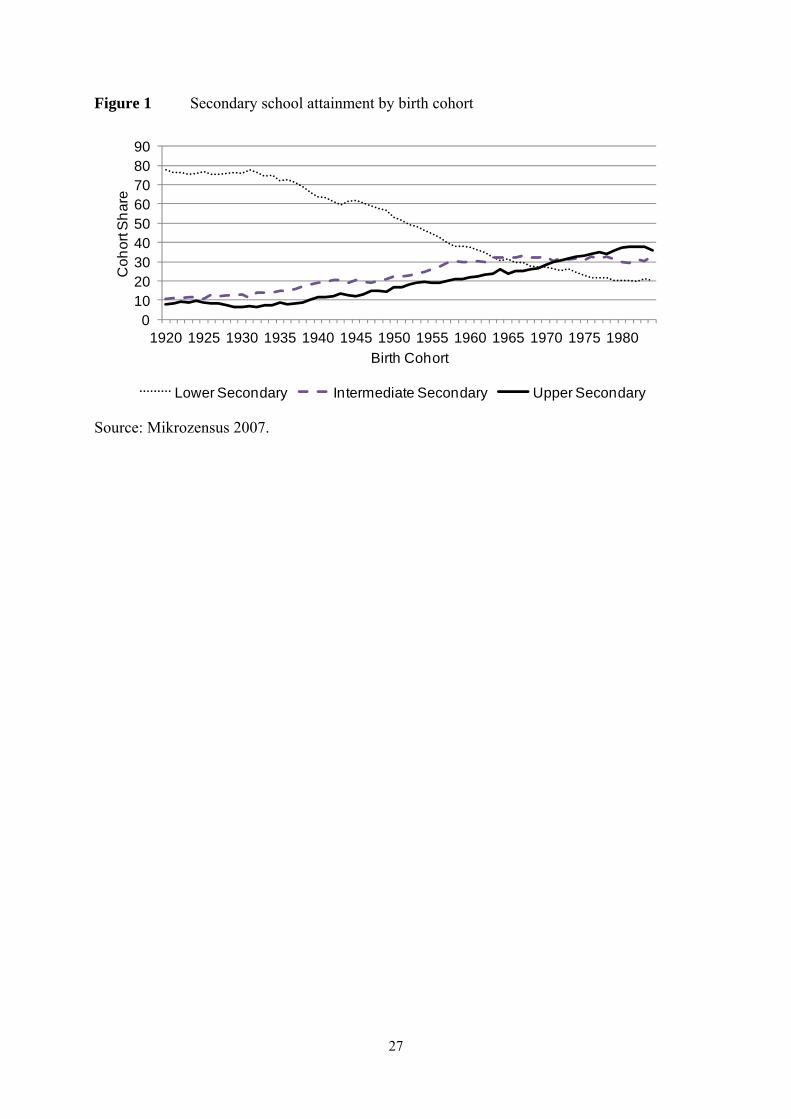
increased starting with the birth cohorts of the late 1930s (see Figure 1). Figure 2 presents

gender-specific cohort shares attaining upper secondary school and academic degrees

beginning with the 1950 birth cohort. In the 1950 birth cohort about 30 percent of males and 15

percent of females attained the upper secondary school degree: these cohort shares increased

for both sexes but with a steeper slope for females (see Figure 2.1). Starting with the 1980 birth

cohort a larger female than male cohort share attained the upper secondary degree. Today, more

than half of male and female birth cohorts attain the degree. Figure 2.2 shows the male and

female cohort shares completing tertiary education: the shares were about constant at 15 percent

for females and 25 percent for males through the mid 1960s birth cohorts. Then they increased,

again with a steeper slope for females. The 1979 birth cohort reached male-female parity at a

cohort share of about 30 percent for both sexes.8

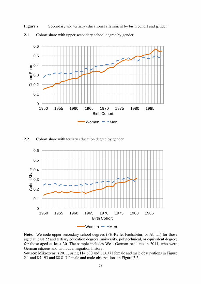
We depict the relative and absolute gender differences in educational attainment in

Figures 3.1 and 3.2. In contrast to evidence for the U.S. (Goldin et al. 2006) the two patterns

look similar: for the birth cohorts of the early 1950s the gender difference in secondary school

attainment exceeded that in academic degrees indicating a higher propensity for females than

males to study conditional on holding the upper secondary school degree. The patterns reversed

by the late 1950s when the difference in secondary school attainment declined rapidly. The

8 We do not show developments for the birth cohorts after 1981 because we conservatively measure tertiary attainment only at age 30 and do not have access to more recent Mikrozensus data.

6

difference in the cohort shares holding academic degrees stayed higher, at an absolute value of

about 7 percentage points throughout the birth cohorts of the 1960s (see Figure 3.2). Our

analysis focuses on this absolute difference.

Before we investigate the mechanisms behind the shift in gender patterns we examine

whether the rise in female educational attainment was equally spread across population groups.

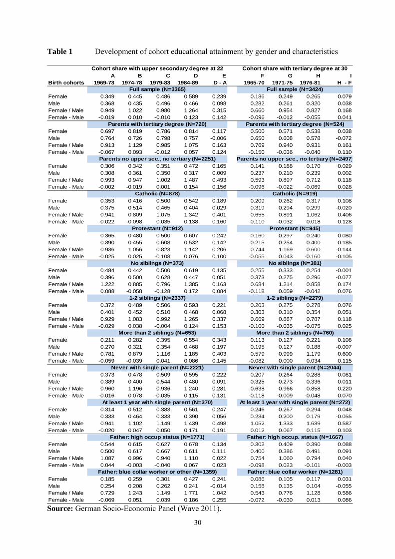
Table 1 presents evidence based on survey data from the German Socio-Economic Panel

(SOEP) which provides individual background information. We evaluate secondary and tertiary

attainment for birth cohorts who have reached age 22 and age 30, respectively. The first rows

show the cohort shares with secondary and tertiary educational attainment by gender and year

of birth. For the full sample we observe an increase of female cohort shares with the upper

secondary school degree over time from 34.9 (column A) to 58.9 percent (column D), whereas

male cohort shares increased from 36.8 to 46.6 percent (again, columns A and D). Column E

summarizes the change over time. The rightmost columns show the development of cohort

shares with tertiary degrees. Again, the female share increased more than male cohort share

(see rows 1 and 2 for columns F, H, and I). The entries in rows 3 and 4 indicate relative and

absolute differences for the two sexes in the respective birth cohort groups. Columns E and I

show that females advanced faster than males for both educational attainments. The relative

'female over male' differences (row 3) rose by 31.5 and 16.8 percentage points, and the absolute

'female minus male' differences (row 4) increased by 14.2 and 4.1 points between the first and

the last cohort group for secondary and tertiary education, respectively.

The next panels describe specific subsamples. We find that the gender difference in

secondary attainment declined more in families with low parental education (i.e., where parents

have neither upper secondary nor tertiary degrees) compared to parents with academic

background. The level differences in educational attainment by parental educational

background are still substantial for both genders in the last cohort group (see columns D and

7

H). More than 75 percent of children of highly educated parents attain upper secondary

education compared to fewer than half of the children of parents with lower education.

Particularly girls in catholic families improved their educational attainment relative to

boys: among Catholics, the female-to-male ratio increased by more than 40 percentage points

for secondary and tertiary attainment. The decline in the gender education gap also varies

depending on whether there are additional siblings in the household; the largest advance in both

secondary and tertiary educational attainment occurred for those with more than two siblings.

Girls growing up in single parent families and those with fathers of low occupational status

advanced the most relative to boys.

Overall, we observe an improvement for females across all population groups; in

contrast, the educational attainment of males did not increase and even declined over time in

some population groups.9 The gender education gap reversed most clearly in favor of females

in disadvantaged circumstances, e.g., with many siblings, in single parent households, with

fathers of low occupational status, and with parents of low educational attainment or catholic

belief. This matches the findings for the U.S. presented by Goldin et al. (2006). In contrast,

Bailey and Dynarski (2011) find that educational advancement and female educational

advantage over males was stronger for those from high-income families. Most of the patterns

that we find are similar for both secondary and tertiary educational attainment.10

9 Our evidence matches the observation of Buchmann and DiPrete (2006) who point to the decline of male educational attainment in situations of absent fathers or of fathers with little education or low occupational status. These authors view the declining rate of male college completion in the U.S. as an important determinant of the educational gender gap reversal. 10 Table 1 looks at different birth cohorts for the analysis of the secondary attainment (1969-1989) and tertiary attainment (1965-1981) for two reasons. First, we assume that completed secondary school attainment can be observed at age 22 and completed tertiary education attainment at age 30. Therefore, the SOEP data of 2011 allow us to study birth cohorts up until 1989 and 1981. Second, we describe only those birth cohorts which we will use in our analysis, where data is available starting in 1984; we assume that the key determinants for secondary school outcomes are observed by age 15 and the factors behind tertiary attainment happen by age 19. Since we can only measure these features starting in 1984, we can go back to birth cohort 1969 in the case of secondary school degrees and to birth cohort 1965 in the case of tertiary education.

8

4. Empirical approach and data

4.1 Empirical approach

We are interested in the sets of factors that are correlated with and potentially explain

the gender education gap and its reversal. Our baseline model for the linear regression of

educational outcomes (Y) is

(1) Yi = β0 + β1 femalei + β2 cohorti + β3 (femalei * cohorti) + δ State FEi + e0i .

Here, β2 describes the mean change in male educational attainment with every new birth cohort

and β3 yields a linear approximation of the gender difference in cohort trends in educational

attainment. If β3 is significant and positive, females' attainment increases faster over time than

males'.11 Since unobserved heterogeneities at the state-level might affect outcomes, we

condition on a set of state fixed effects. Our strategy is to add explanatory variables (X) to the

model that might be associated with the difference in trends for males and females and thus

may reduce the magnitude and statistical significance of the estimate of β3:

(2) Yi = β0 + β1 femalei + β2 cohorti + β3 (femalei * cohorti) + β4 X'i + δ State FEi + e1i .

Following the literature, we focus on four groups of indicators for X: (a) individual

characteristics, (b) labor market characteristics, (c) characteristics of state education systems,

and (d) other characteristics such as state-level demographics and social norms (for a detailed

list of the considered indicators, please see Appendix A). Also, we consider interactions of the

characteristics X with the 'female' indicator to allow for gender-specific differences in the

correlations of X with educational attainment:

(3) Yi = β0 + β1 femalei + β2 cohorti + β3 (femalei * cohorti)

+ β4 X'i + β5 (femalei * X'i) + δ State FEi + e2i .

11 In principle, the time trend could be specified in a more flexible way. However, as Figure 2 suggests that the developments are almost linear and because the interpretation of linear trends is much clearer we prefer the simple linear specification.

9

We investigate whether the consideration of control variables and their gender-interaction

effects affects the estimates of β3: if we obtain a statistically significant estimate of β3 based on

equation (1) and if adding a control variable X renders the estimate of β3 small and/or

insignificant then we consider the control variable X to be correlated with the gender education

gap and therefore with its development over time and reversal.12 Generally, we use

heteroscedasticity-robust standard errors.13 In robustness tests we extend the specification by

adding controls for X-by-cohort interactions, for state fixed effects by cohort interactions, and

for both additional controls jointly. Also, we estimate our models on grouped data at the state-

by-gender-by-cohort level.

4.2 Sample and covariates

We use data from the German Socio-Economic Panel (SOEP) (Wagner et al. 2007). The

SOEP offers rich individual and parental background data, which we supplement with

information from official statistics. Our sample considers West German natives and second

generation immigrants who grew up in West Germany. We use the cross-section of individuals

interviewed in 2011 which allows us to also consider recent birth cohorts.

We analyze three binary outcome variables: graduation from upper secondary school,

entry to tertiary education ("any tertiary"), and completion of a tertiary degree.14 These

measures describe separate education outcomes that are determined at different stages in the

life cycle; clearly, not all upper secondary school graduates start tertiary education, and not all

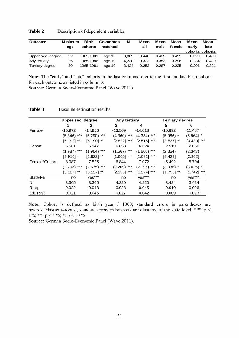
who start successfully complete it. Table 2 describes the dependent variables and their

respective samples. We measure each outcome imposing age limitations on the sample; in

12 Strictly speaking, X would only be correlated with the gender difference in time trends, however, eventually that determines the reversal of the gender gap. 13 Considering random effects at the family level does not affect our results. We prefer robust standard errors because they allow for more general error term correlation patterns. 14 Goldin et al. (2006) and Bailey and Dynarski (2011) similarly study college entry and college completion. In the German educational system, upper secondary school attainment is more relevant than in the U.S. because it can present an entry barrier to tertiary education.

10

particular, we check among those who are at least 22 years old whether they hold the upper

secondary school degree, among those aged at least 25 whether they ever started tertiary

education, and among those aged at least 30 whether they hold a tertiary degree. Given that our

data were gathered in 2011 this defines the youngest considered birth cohorts available for each

outcome as 1989, 1986, and 1981, respectively.

To explain educational choices we match information that was available when the

person decided to pursue a degree: we pick age 15, i.e., about grade ten, to match information

that may have been relevant for the decision to attend upper secondary school, and age 19 to

match information that may have been relevant for the decision to pursue tertiary education.

The SOEP provides data since 1984. Given the matching ages 15 and 19, this determines as the

oldest birth cohorts considered in our analyses, 1969 and 1965 for the secondary and tertiary

outcomes, respectively. In all cases our samples comprise more than 3,000 observations. Table

2 shows the overall means, the means by gender, and for early and late birth cohorts. In our

sample, the share of females holding the upper secondary school degree exceeds the share of

males while males on average still predominate with respect to tertiary education. The two

rightmost columns confirm increases in educational attainment over time.

5. Results

5.1 Approach and baseline results

We present our results in two steps. First, we discuss the baseline results of model (1)

for the three outcomes. In step two, we separately consider the association of four sets of

characteristics (X) with the development of the gender education gap using models (2) and (3);

we differentiate the role of (i) individual characteristics (e.g., family background or religion),

(ii) regional labor market characteristics (e.g., wage returns to education or state

unemployment), (iii) state education systems (e.g., class size and share of female teachers) and,

finally, (iv regional demographics (e.g., divorce, marriage, and fertility rates) and social norms.

11

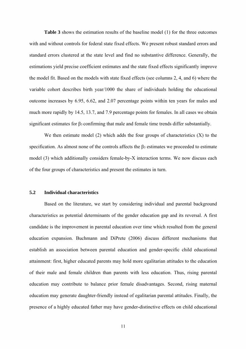
Table 3 shows the estimation results of the baseline model (1) for the three outcomes

with and without controls for federal state fixed effects. We present robust standard errors and

standard errors clustered at the state level and find no substantive difference. Generally, the

estimations yield precise coefficient estimates and the state fixed effects significantly improve

the model fit. Based on the models with state fixed effects (see columns 2, 4, and 6) where the

variable cohort describes birth year/1000 the share of individuals holding the educational

outcome increases by 6.95, 6.62, and 2.07 percentage points within ten years for males and

much more rapidly by 14.5, 13.7, and 7.9 percentage points for females. In all cases we obtain

significant estimates for β3 confirming that male and female time trends differ substantially.

We then estimate model (2) which adds the four groups of characteristics (X) to the

specification. As almost none of the controls affects the β3 estimates we proceeded to estimate

model (3) which additionally considers female-by-X interaction terms. We now discuss each

of the four groups of characteristics and present the estimates in turn.

5.2 Individual characteristics

Based on the literature, we start by considering individual and parental background

characteristics as potential determinants of the gender education gap and its reversal. A first

candidate is the improvement in parental education over time which resulted from the general

education expansion. Buchmann and DiPrete (2006) discuss different mechanisms that

establish an association between parental education and gender-specific child educational

attainment: first, higher educated parents may hold more egalitarian attitudes to the education

of their male and female children than parents with less education. Thus, rising parental

education may contribute to balance prior female disadvantages. Second, rising maternal

education may generate daughter-friendly instead of egalitarian parental attitudes. Finally, the

presence of a highly educated father may have gender-distinctive effects on child educational

12

attainment; typically, the attainment of sons responds more strongly to the absence of a father

than the attainment of girls (see also Table 1 on single parent households).15

Various authors point to heterogeneities in educational outcomes based on the

availability of parental resources. We know that firstborn children are at an advantage compared

to later born siblings and we know that children in large families have to share parental

resources with more competitors than children without siblings (e.g., de Haan 2010, Eschelbach

2014). Similarly, the income situation is on average better in households with two income

earning parents than in single parent households.16 Therefore we investigate whether changes

in household size and structure are associated with the gender education gap and its reversal.17

Also, we consider the relevance of parental migration experience. There is evidence that

intergenerational mobility differs by immigrant status (Bauer and Riphahn 2007) and that

attitudes to educational advancement differ between natives and immigrants (Buchmann and

DiPrete 2006). Both mechanisms may affect the gender education gap, given rising population

shares of immigrants in Germany.

Finally, we consider a set of controls for religious affiliation and church attendance. The

heterogeneity between Christian and non-Christian beliefs may approximate the native-

immigrant divide, as the majority of West German natives are of Christian belief. Also, Table

1 shows considerable differences in child educational attainment, its development over time,

and the gender education gap between Catholics and Protestants.18 Traditionally, female

15 Legewie and DiPrete (2009) discuss differences in the role of parental education for the gender education gap in the United States and Germany. Christofides et al. (2010) show that changes in parental education yield different effects for males and females in Canadian higher education. 16 Autor et al. (2014) show a clear connection between single parent households and the gender education gap in the U.S.. 17 In addition to the estimates presented in Table 4.1 we considered alternative specifications with various interaction terms of birth order and sibship size. However, the key results are highly robust to variations in these controls. 18 Based on the 2011 census roughly 30 percent of the German population are catholic, 30 percent are protestant, and 40 percent "nothing or other". In West Germany a population share of about 40 percent is catholic and protestant, each.

13

education was valued more by Protestants than Catholics (Becker and Wößmann 2008); this

suggests that any changes over time, e.g., in social norms, may differ across denominations.

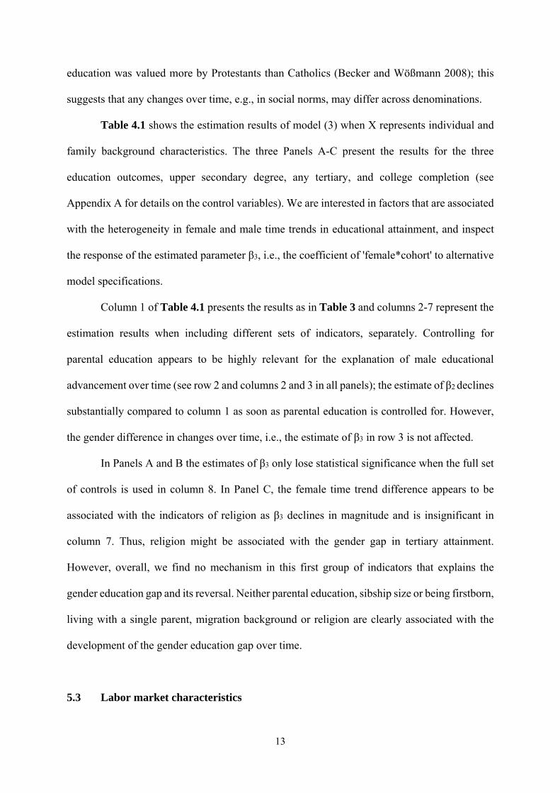
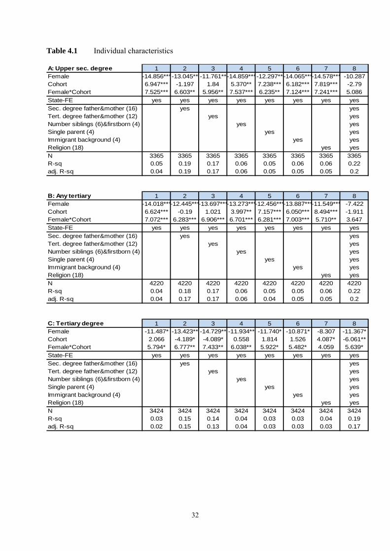
Table 4.1 shows the estimation results of model (3) when X represents individual and

family background characteristics. The three Panels A-C present the results for the three

education outcomes, upper secondary degree, any tertiary, and college completion (see

Appendix A for details on the control variables). We are interested in factors that are associated

with the heterogeneity in female and male time trends in educational attainment, and inspect

the response of the estimated parameter β3, i.e., the coefficient of 'female*cohort' to alternative

model specifications.

Column 1 of Table 4.1 presents the results as in Table 3 and columns 2-7 represent the

estimation results when including different sets of indicators, separately. Controlling for

parental education appears to be highly relevant for the explanation of male educational

advancement over time (see row 2 and columns 2 and 3 in all panels); the estimate of β2 declines

substantially compared to column 1 as soon as parental education is controlled for. However,

the gender difference in changes over time, i.e., the estimate of β3 in row 3 is not affected.

In Panels A and B the estimates of β3 only lose statistical significance when the full set

of controls is used in column 8. In Panel C, the female time trend difference appears to be

associated with the indicators of religion as β3 declines in magnitude and is insignificant in

column 7. Thus, religion might be associated with the gender gap in tertiary attainment.

However, overall, we find no mechanism in this first group of indicators that explains the

gender education gap and its reversal. Neither parental education, sibship size or being firstborn,

living with a single parent, migration background or religion are clearly associated with the

development of the gender education gap over time.

5.3 Labor market characteristics

14

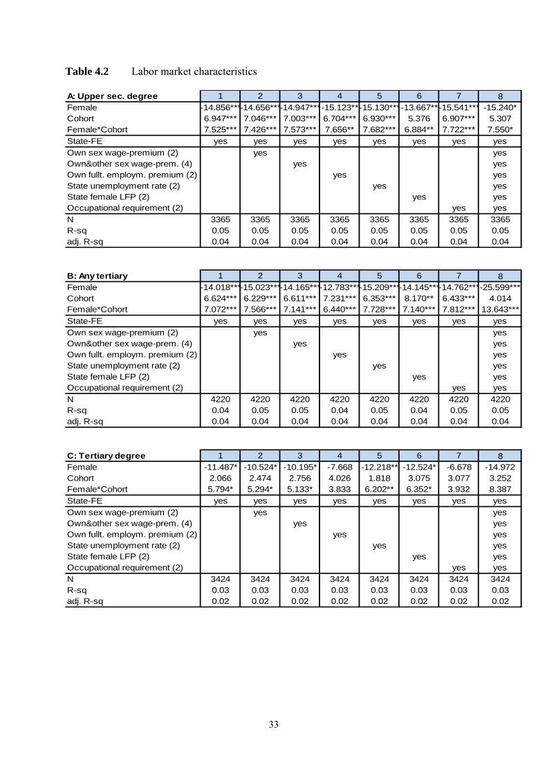
Next, we study the association of the gender education gap with labor market

characteristics. We focus on six potentially relevant indicators. The wage return to education is

generally considered to be a key benefit of higher education and many contributions discuss

whether its level and development explain the trend of the gender gap in educational attainment

(e.g., Hubbard 2011). We code medium-run fulltime earnings differences with and without

upper secondary or tertiary degrees by sex, calendar year, and federal state and match them to

the data. Because numerous authors discuss marriage market advantages as an important benefit

of higher education (e.g., Bailey and Dynarksi 2011, DiPrete and Buchmann 2006, or Goldin

et al. 2006), we additionally consider the returns to education of the opposite sex as an

explanatory variable.

Goldin et al. (2006) point out that shifts in female labor market participation

expectations affect education choices. Therefore we code as a "full-time employment premium"

the mean difference in the number of years in full-time employment (up to age 35) that is

connected with upper secondary or tertiary education. We differentiate by sex, birth cohort and

federal state and use the indicator in the estimations. Since labor market characteristics such as

the state unemployment rate or state female labor force participation may affect human capital

investments and females' expectations regarding the relevance of education for their life cycle

labor market opportunities, we consider them as well.

We code our last indicator, occupational requirement, in response to the observation

that gender-specific shifts in job tasks over time, in particular the decline in routine tasks for

females, contributed to the closing of the gender wage gap (Black and Spitz-Oener 2010,

Beaudry and Lewis 2014). In order to measure possible gender-specific shifts in educational

requirements for occupations we calculated for men and women the average number of

'occupation-specific years of schooling' among job starters weighted by the gender-specific

frequency of occupations: if, e.g., the educational requirements of 'female occupations'

15

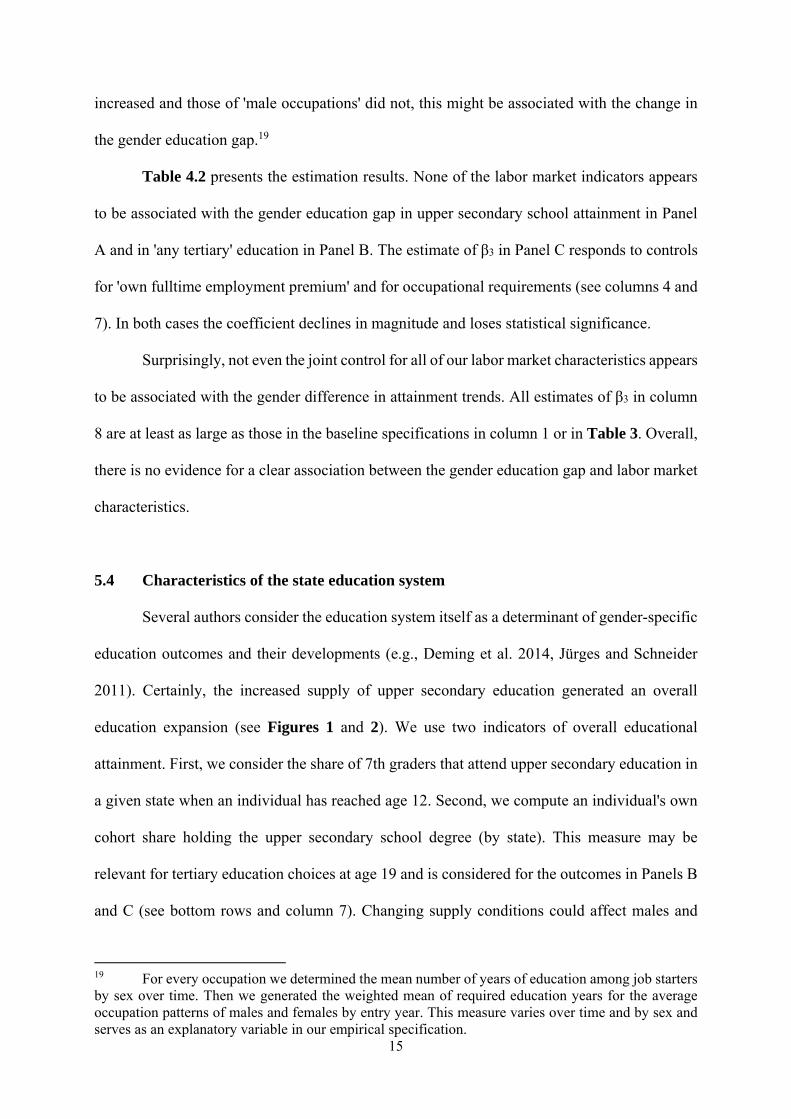
increased and those of 'male occupations' did not, this might be associated with the change in

the gender education gap.19

Table 4.2 presents the estimation results. None of the labor market indicators appears

to be associated with the gender education gap in upper secondary school attainment in Panel

A and in 'any tertiary' education in Panel B. The estimate of β3 in Panel C responds to controls

for 'own fulltime employment premium' and for occupational requirements (see columns 4 and

7). In both cases the coefficient declines in magnitude and loses statistical significance.

Surprisingly, not even the joint control for all of our labor market characteristics appears

to be associated with the gender difference in attainment trends. All estimates of β3 in column

8 are at least as large as those in the baseline specifications in column 1 or in Table 3. Overall,

there is no evidence for a clear association between the gender education gap and labor market

characteristics.

5.4 Characteristics of the state education system

Several authors consider the education system itself as a determinant of gender-specific

education outcomes and their developments (e.g., Deming et al. 2014, Jürges and Schneider

2011). Certainly, the increased supply of upper secondary education generated an overall

education expansion (see Figures 1 and 2). We use two indicators of overall educational

attainment. First, we consider the share of 7th graders that attend upper secondary education in

a given state when an individual has reached age 12. Second, we compute an individual's own

cohort share holding the upper secondary school degree (by state). This measure may be

relevant for tertiary education choices at age 19 and is considered for the outcomes in Panels B

and C (see bottom rows and column 7). Changing supply conditions could affect males and

19 For every occupation we determined the mean number of years of education among job starters by sex over time. Then we generated the weighted mean of required education years for the average occupation patterns of males and females by entry year. This measure varies over time and by sex and serves as an explanatory variable in our empirical specification.

16

females differently if the genders respond differently to changes in the signal value of

education. If the signal value of the upper secondary school degree declines when a larger

cohort share holds it, more individuals then may move on to tertiary education (Bedard 2001).

If the cost of education differs by gender (Becker et al. 2010) females might respond more

strongly to this shifting signal value than males. This could explain the change in the gender

education gap.

One mechanism that is broadly discussed as a possible source of gender differences is

the share of female teachers (Nixon and Robinson 1999). Bailey and Dynarski (2011)

differentiate the effect of having a role model and the effect of gender biases in teacher

behaviors that may result in different outcomes for boys and girls in the class room. If the share

of female teachers changed over time this may alter gender-specific education outcomes. We

consider the share of females among all teachers in elementary/lower secondary schools and in

upper secondary schools, by state and year.20

Finally, there is a broad literature on the beneficial effect of small class size on

educational attainment (e.g., Mueller 2013). De Giorgi et al. (2012) and Dearden et al. (2002)

show that the impact of class size on student performance can differ for males and females.21

Therefore, changes in class sizes over time may affect the gender education gap and its reversal.

We use indicators of average class size in elementary school and in grades 7 and 8 at upper

secondary schools by state and year to investigate this mechanism.

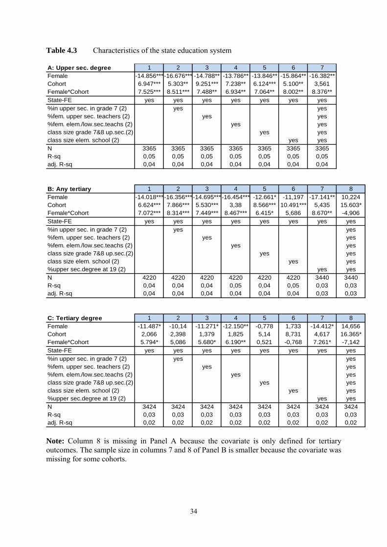
Table 4.3 shows the estimation results for our three outcomes. None of the education

indicators appears to be associated with the gender education gap in upper secondary school

attainment in Panel A. The estimate of β3 in Panel B declines in magnitude and turns

insignificant in column 6 where we control for class size. The same holds for the results in

20 We also control for the share of female taught hours. The results did not differ from those presented (available upon request). 21 For additional evidence on differential response to educational quality by gender, see Lavy (2011) or Deming et al. (2014).

17

columns 5 and 6 in Panel C. These results, which are identified based on the heterogeneity in

class sizes within states over time, suggest that the advance of females' academic achievement

is associated with the trend to smaller classes in both elementary school and early upper

secondary school.22 Our results are in contrast to those of De Giorgi et al. (2012) who study the

effect of tertiary education class sizes on tertiary education outcomes and find larger benefits

for men. Our finding of beneficial class size effects for females confirms Deming et al. (2014,

p.1010) who conclude "that girls are more responsive than boys to gains in school quality." In

addition, the estimates of β3 in Panel C turn insignificant when we control for 'supply effects',

i.e., the cohort share in upper secondary education in grade 7 (see column 2).

In Table 4.3 the joint model in the rightmost column does not affect the estimate of β3

substantially in Panel A; however, it yields a reversal of the gender-specific trends in Panels B

and C. Overall, the gender education gap in tertiary education and its reversal appear to be

associated most closely with the availability of upper secondary education and with class size.

5.5 Demographics and social norms

As our final group of characteristics we consider demographics such as divorce,

marriage, and fertility rates, and indicators of social norms, all measured at the state-by-year

level. We measure these covariates in the period when individuals make educational choices,

i.e., at age 15 for Panel A and at age 19 for Panels B and C.

Numerous authors discuss the relevance of these measures for female education choices

(e.g., Goldin et al. 2006, Buchmann and DiPrete 2006, Bronson 2013). The shifts to delayed

marriage, reduced fertility, and increased divorce rates may affect females' education choices:

if, e.g., marriage rates decline, the probability of being able to rely on the financial support of

22 The mean class sizes in elementary school / grades 7 and 8 in upper secondary school for the samples used in Panel C of Table 4.3 indeed declined over time: for birth cohort 1965 we observe 28.9 / 31.5, for birth cohort 1975 22.2 / 25.1, and for birth cohort 1981 21.5 / 25.8 pupils per class.

18

a husband declines. Similarly, rising divorce rates increase the relevance of economic

independence (e.g., Fernandez and Wong 2014). These developments incentivize investments

in human capital.

In Germany these demographic shifts came along with substantial changes in social

norms and attitudes regarding the role of women. We gather information on attitudes from the

ALLBUS surveys where respondents were asked regularly whether women should give up their

job after getting married and whether women should stay at home and look after their kids

(Koch and Wasmer 2004). The share of individuals agreeing with these statements dropped

from 57 percent in the 1982 survey to below 30 percent in 2008. We evaluate whether this shift

in social norms is associated with the gender education gap and its reversal in Germany. The

connection between norms and education choices is asserted in numerous studies (e.g., Parro

2012, Goldin et al. 2006, Bailey and Dynarski 2006, Christofides et al. 2010, Legewie and

DiPrete 2009).

Table 4.4 presents our results. In Panel A the estimate of β3 turns insignificant when

controls for state divorce rates (column 2) and social norms (column 5) are considered.

However, the latter control renders the coefficient substantially larger in size. In Panel B only

the change in norms appears to be associated with the shift in the gender education gap: the

estimate of β3 in column 5 turns negative and insignificant. The same holds in Panel C. The

shift in social norms is the only mechanism which generates an insignificant estimate of β3 for

all three outcomes. In addition, in Panel C the estimate of β3 declines in magnitude and turns

insignificant when we control for the state fertility rate measured at the time when young

women take tertiary educational choices (see column 4). Overall, state divorce rates, fertility

rates, and particularly social attitudes regarding the role of women appear to be associated with

the gender education gap and its reversal.

6. Robustness Tests

19

To investigate the robustness of our results we follow three pathways: first we apply

alternative and more flexible model specifications, second we acknowledge that many

covariates vary at the state-by-year level and re-estimate our models on grouped 'state-by-year-

by-sex' data. Finally, we address potential measurement problems and consider alternative

definitions of our indicators. We discuss the findings in turn.

As a first set of robustness tests we added further controls to the specification of model

(3). Specifically, we considered state-specific cohort trends, interactions of the control variables

(X) with cohort trends, and both additions jointly. The results are available upon request. The

estimates generally confirm prior findings: religion, the own fulltime employment premium,

occupational requirements, class size, fertility rates, and conservative attitudes are associated

with the gender-specific trends in attaining a tertiary degree; class size in elementary school

and conservative attitudes are correlated with the trends in attending tertiary education, and we

continue to find that none of the individual level and state education system characteristics are

associated with gender differences in the trends of attaining the upper secondary school degree.

Additionally, we find some support for an association of the own fulltime employment premium

for all three dependent variables, and we find that the state divorce rate may be associated with

upper secondary school trends once the time trend interactions of the indicators (X) are

considered. However, the only controls that render the estimate of β3 not only statistically but

also economically insignificant, i.e., reduce it to close to zero or even negative, continue to be

class size and conservative attitudes for the tertiary degree outcome. Therefore we consider

these two indicators to reflect the mechanisms which are most closely associated with the steep

increase in female to male education ratio.

In a second robustness test we address the fact that several of our indicators are collected

at the 'state-by-year' level. To determine whether the findings are connected to the weighting of

subgroups of individuals we generated a pooled sample of mean values of all characteristics at

the 'state-by-cohort-by-sex' level. The estimation results are provided in Appendix B. Column

20

1 of Table B.1 shows that in these smaller samples we still obtain large differences between

educational trends for males and females. The difference is statistically significant only for the

"any tertiary" outcome (see column 1 of Panel B); however, Panels A and C also yield faster

growth for females than for males. Panel C shows no overall growth in tertiary education for

males over time. We redo the analysis with the four groups of indicators as in Tables 4.1-4.4.

Among the individual level characteristics (see Table B.1) the single parent indicator now

appears to be most able to reduce the estimate of β3 to near zero or negative value.23 Table B.2

confirms that the own fulltime employment premium may be (weakly) correlated with the

female education cohort trend. In Table B.3 we find additional evidence supporting the role of

class sizes as a driver of relative female educational advancement, particularly at the tertiary

level. Table B.4 shows that the evidence on the role of social norms is robust to the change in

the sample. Therefore overall, the additional estimations confirm previous results.

Finally, we redefine a number of variables to ensure that the results are not the outcome

of specific measurement choices. We use alternative specifications such as divorce rates per

inhabitant vs. per marriage, considered the share of female taught lessons in addition to and

instead of the share of female teachers. So far we used wage and employment premiums based

on averages of observed values; additionally we applied regression estimates of premiums using

various specifications with alternative regional and age controls. We did not find substantial

sensitivity of the results to our measurement choices.

7. Conclusions

23 The coefficient estimates for the model of column 5 of Panel A show a significant negative association between growing up with a single parent and attaining the upper secondary school degree. This association is larger for boys than for girls. This result is identical for the pooled data and the individual level data of Tables B.1 and 4.1. Over time the average time which youths spent in single parent households increased from about 5 months for the birth cohort of 1969 to about 14 months for the birth cohort of 1989.

21

This paper describes the reversal of the gender education gap in Germany and

investigates mechanisms that may explain it. Up until the birth cohort of 1979 the educational

attainment of males in secondary and tertiary education exceeded that of females. Since then

females increasingly outperform males. This phenomenon is observed in almost all advanced

economies (Parro 2012) and various studies have investigated the shift in college entry,

persistence, and completion for the United States.

The reversal of the gender education gap in Germany appears to be most pronounced in

disadvantaged population groups: relative to their male peers, female secondary and tertiary

education caught up the most in families with many children, in single parent households, in

families with fathers of low occupational status, and in catholic households.

We investigate the mechanisms behind the the gender education gap and its reversal for

three outcomes: attainment of the upper secondary school degree, any tertiary education, and

completed tertiary education. We test the association of four groups of characteristics with

gender trend differences: individual and family background, labor market indicators,

characteristics of the education system, and state demographics and social norms. The results

vary somewhat across outcomes. Our major findings on potential determinants of the German

gender education gap and its reversal are as follows:

None of the individual and family background variables contributes substantially to an

explanation of the reversal of the gender education gap when we use individual level data.24 In

an analysis using grouped data we find that living with a single parent is associated with the

gender difference in education trends. Two interpretations may be relevant. First, we know from

prior studies that boys' educational attainment suffers more than girls' educational attainment

from the absence of a father (Bertrand and Pan 2013). A rising share of single parent households

24 Clearly, changes in unobserved heterogeneities such as the allocation of time and resources between male and female children may have changed over time but cannot be investigated due to the lack of information.

22

thus may hurt boys' attainment. Second, once information on economic risks in life becomes

salient, girls may respond more strongly than boys and intensify their investments in human

capital. After all, they see the mother as the typical single parent and gender differences in risk

aversion may be at work. Numerous studies have discussed the insurance value of education

for women (see Bronson 2013 and literature cited there). Through this mechanism the rising

share of single parent households may − at least in principle − increase girls' (relative)

educational attainment.

We find surprisingly little evidence of an association between the gender education gap

and the labor market. Wage returns to education, state unemployment, and female labor force

participation rates appear to be correlated with the gender education gap. Two indicators seem

to be weakly associated with the development of the gender education gap in tertiary degrees

over time: the 'own educational employment premium', i.e., the expected increase in fulltime

employment following educational achievement, and the occupation-specific educational

requirements over time. This suggests that female tertiary education choices respond to the

demands of the labor market.

Interestingly, the only characteristic of state education systems that is associated with

the gender education gap and its reversal (at the tertiary level) is not the increase in upper

secondary school supply but the development of secondary school class sizes over time. This

suggests that females benefit more from the decline in class sizes over time confirming Deming

et al. (2014). If investments in educational quality affect males and females differently, future

studies of the causal effects of educational reforms should add a focus on gender differences.

Finally, demographics such as marriage, divorce, and fertility rates are not central to the

gender education gap and its reversal. Pooled data confirm a weak contribution of the drop in

fertility to explain the shift in secondary school attainment, and individual data find a slim

contribution of divorce rates. These correlations, however, are weak at best. Much stronger is

the correlation of the gender education gap with our measure of social norms: controlling for

23

social norms that persisted at the time when educational choices are made contributes

substantially to explain the shift in tertiary educational attainment. Across all considered

mechanisms, the change in social norms (plus the relevance of reduced class sizes) appears to

be most closely associated with the reversal of the gender education gap at the level of tertiary

education in Germany. Clearly, an economic interpretation of this correlation is challenging for

various reasons. However, reverse causality appears unlikely as the attitudes are measured for

the entire society and are then related to the educational choice of 15 and 19 years olds.

24

Bibliography Ammermüller, Andreas and Andrea Maria Weber, 2005, Educational Attainment and Returns

to Education in Germany, ZEW Discussion Paper No. 05-17, ZEW Mannheim. Autor, David H., David Figlio, Krzysztof Karbownik, Jeffrey Roth, and Melanie Wasserman,

2014, Family Structure and the Gender Gap in Educational and Behavioral Outcomes, mimeo, MIT and Northwestern University.

Bailey, Martha J. and Susan M. Dynarski, 2011, Gains and gaps: changing inequality in U.S. college entry and completion, NBER Working Paper No. 17633, Cambridge MA.

Bauer, Philipp and Regina T. Riphahn, 2007, Heterogeneity in the Intergenerational Transmission of Educational Attainment: Evidence from Switzerland on Natives and Second Generation Immigrants, Journal of Population Economics 20(1), 121-148.

Beaudry, Paul and Ethan Lewis, 2014, Do Male-Female Wage Differentials Reflect Differences in the Return to Skill? Cross-City Evidence from 1980-2000, American Economic Journal: Applied Economics 6(2), 178-194.

Becker, Gary S., William H.J. Hubbard, and Kevin M. Murphy, 2010, Explaining the Worldwide Boom in Higher Education of Women, Journal of Human Capital 4(3), 203-241.

Becker, Sascha O. and Ludger Wößmann, 2008, Luther and the Girls: Religious Denomination and the Female Education Gap in 19th Century Prussia, Scandinavian Journal of Economics 110(4), 777-805.

Bedard, Kelly, 2001, Human Capital vs. Signaling Models: University Access and High School Dropouts, Journal of Political Economy 109(4), 749-775.

Bertocchi, Graziella and Monica Bozzano, 2014, Family Structure and the Education Gender Gap: Evidence from Italian Provinces, IZA Discussion Paper No. 8347, IZA Bonn.

Bertrand, Marianne and Jessica Pan, 2013, The Trouble with Boys: Social Influences and the Gender Gap in Disruptive Behavior, American Economic Journal: Applied Economics 5(1), 32-64.

Black, Sandra E. and Alexandra Spitz-Oener, 2010, Explaining women's success: technological change and the skill content of women's work, Review of Economics and Statistics 92(1), 187-194.

Boockmann, Bernhard and Viktor Steiner, 2006, Cohort effects and the returns to education in West Germany, Applied Economics 38, 1135-1152.

Bronson, 2013, Degrees are forever: marriage, educational investment, and lifecycle labor decisions of men and women, mimeo, UCLA, Los Angeles.

Buchmann, Claudia and Thomas A. DiPrete, 2006, The Growing Female Advantage in College Completion: The Role of Family Background and Academic Achievement, American Sociological Review 71(4), 515-541.

Charles, Kerwin Kofi and Ming-Ching Luoh, 2003, Gender differences in completed schooling, Review of Economics and Statistics 85(3), 559-577.

Cho, Donghun, 2007, The role of high school performance in explaining women's rising college enrollment, Economics of Education Review 26(4), 450-462.

Christofides, Louis N., Michael Hoy, and Ling Yang, 2010, Participation in Canadian Universities: The gender imbalance (1977-2005), Economics of Education Review 29(3), 400-410.

De Giorgi, Giacomo, Michele Pellizzari, and William Gui Woolston, 2012, Class Size and Class Heterogeneity, Journal of the European Economic Association 10(4), 795-830.

Dearden, Lorraine, Javier Ferri, and Costas Meghir, 2002, The effect of school quality on educational attainment and wages, Review of Economics and Statistics 84(1), 1-20.

De Haan, Monique, 2010, Birth order, family size and educational attainment, Economics of Education Review 29(4), 576-588.

25

Deming, David J., Justine S. Hastings, Thomas J. Kane, and Douglas O. Staiger, 2014, School Choice, School Quality, and Postsecondary Attainment, American Economic Review 104(3), 991-1013.

DiPrete, Thomas A. and Claudia Buchmann, 2006, Gender-specific trends in the value of education and the emerging gender gap in college completion, Demography 43(1), 1-24.

Eschelbach, Martina, 2014, Crown Princes and Benjamins: Birth Order and Educational Attainment in East and West Germany, forthcoming: Journal of Economics and Statitistics (Jahrbücher für Nationalökonomie und Statistik).

Fernandez, Raquel and Joyce Wong, 2014, Unilateral Divorce, the Decreasing Gender Gap and Married Women's Labor Force Participation, American Economic Review 104(5), 342-347.

Fitzenberger, Bernd and Karsten Kohn, 2006, Skill Wage Premia, Employment, and Cohort Effects: Are Workers in Germany All of the Same Type?, IZA Discussion Paper No. 2185, IZA, Bonn.

Gebel, Michael and Friedhelm Pfeiffer, 2010, Educational expansion and its heterogeneous returns for wage workers, Schmollers Jahrbuch 130(1), 19-42.

Goldin, Claudia, Lawrence F. Katz, and Ilyana Kuziemko, 2006, The Homecoming of American College Women: The Reversal of the College Gender Gap, Journal of Economic Perspectives 20(4), 133-156.

Hubbard, William H.J., 2011, The Phantom Gender Difference in the College Wage Premium, Journal of Human Resources 46(3), 568-586.

Jürges, Hendrik and Kerstin Schneider, 2011, Why Young Boys Stumble: Early Tracking, Age and Gender Bias in the German School System, German Economic Review 12(4), 371-394.

KMK (Kultusministerkonferenz), 2013, The Education System in the Federal Republic of Germany 2011/2012, Secretariat of the Standing Conference of the Ministers of Education and Cultural Affairs of the Länder in the Federal Republic of Germany, Bonn. [www.kmk.org/fileadmin/doc/Dokumentation/Bildungswesen_en_pdfs/dossier_en_ebook.pdf - last accessed Sept. 11, 2014]

Koch, Achim and Martina Wasmer, 2004, Der ALLBUS als Instrument zur Untersuchung sozialen Wandels. In: Schmitt-Beck, R.; Wasmer, M.; Koch, A. (eds.), Sozialer und politischer Wandel in Deutschland. Analysen mit ALLBUS-Daten aus zwei Jahrzehnten. 2004, Wiesbaden: VS Verlag für Sozialwissenschaften, pp. 13-41.

Lavy, Victor, 2011, What makes an effective teacher? Quasi-experimental evidence, NBER Working Paper No. 16885, NBER Cambridge, Massachusetts.

Legewie, Joscha and Thomas A. DiPrete, 2009, Family Determinants of the Changing Gender Gap in Educational Attainment: A Comparison of the U.S. and Germany, Schmollers Jahrbuch (Journal of Applied Social Science Studies) 129(2), 169-180.

Mueller, Steffen, 2013, Teacher experience and the class size effect - Experimental evidence, Journal of Public Economics 98(C), 44-52.

Nixon, Lucia A. and Michael D. Robinson, 1999, The educational attainment of young women: role model effects of female high school faculty, Demography 36(2), 185-194.

Parro, Francisco, 2012, International Evidence on the Gender Gap in Education over the Past Six Decades: A Puzzle and an Answer to It, Journal of Human Capital 6(2), 150-185.

Pekkarinen, Tuomas, 2008, Gender Differences in Educational Attainment: Evidence on the Role of Tracking from a Finnish Quasi-experiment, Scandinavian Journal of Economics 110(4), 807-825.

Riphahn, Regina T., 2011, Effect of secondary school fees on educational attainment, Scandinavian Journal of Economics 114(1), 148-176.

26

Riphahn, Regina T. and Michael J. Zibrowius, 2015, Apprenticeship, Vocational Training and Early Labor Market Outcomes - Evidence from East and West Germany, forthcoming Education Economics.

Schnabel, Isabel and Reinhold Schnabel, 2002, Family and Gender Still Matter: The Heterogeneity of Returns to Education in Germany, ZEW Discussion Paper No. 02-67, ZEW Mannheim.

STBA (Statistisches Bundesamt), 2012, Statistisches Jahrbuch 2012, Wiesbaden. Wagner, Gert G., Joachim. R. Frick, and Jürgen. Schupp, 2007, The German Socio-Economic

Panel Study (SOEP) - Scope, Evolution and Enhancemants,” Schmollers Jahrbuch (Journal of Applied Social Science Studies), 127, 139–69, 2007.

27

Figure 1 Secondary school attainment by birth cohort

0102030405060708090

1920 1925 1930 1935 1940 1945 1950 1955 1960 1965 1970 1975 1980

Co

ho

rt S

ha

re

Birth Cohort

Lower Secondary Intermediate Secondary Upper Secondary

Source: Mikrozensus 2007.

28

Figure 2 Secondary and tertiary educational attainment by birth cohort and gender

2.1 Cohort share with upper secondary school degree by gender

0

0.1

0.2

0.3

0.4

0.5

0.6

1950 1955 1960 1965 1970 1975 1980 1985

Co

ho

rt S

ha

re

Birth Cohort

Women Men

2.2 Cohort share with tertiary education degree by gender

0

0.1

0.2

0.3

0.4

0.5

0.6

1950 1955 1960 1965 1970 1975 1980 1985

Co

ho

rt S

ha

re

Birth Cohort

Women Men

Note: We code upper secondary school degrees (FH-Reife, Fachabitur, or Abitur) for those aged at least 22 and tertiary education degrees (university, polytechnical, or equivalent degree) for those aged at least 30. The sample includes West German residents in 2011, who were German citizens and without a migration history. Source: Mikrozensus 2011, using 114.630 and 113.371 female and male observations in Figure 2.1 and 85.193 and 88.813 female and male observations in Figure 2.2.

29

Figure 3 Relative and absolute gender differences in attainment by cohort

3.1 Ratio of male-to-female attainment rates by cohort and educational level

0.0

0.2

0.4

0.6

0.8

1.0

1.2

1.4

1.6

1.8

2.0

1950 1955 1960 1965 1970 1975 1980 1985

Ma

le-t

o-F

em

ale

Ra

tio

Birth Cohort

Upper Secondary School Tertiary Education

3.2 Difference of male and female attainment rates by cohort and educational level

-0.15

-0.10

-0.05

0.00

0.05

0.10

0.15

1950 1955 1960 1965 1970 1975 1980 1985

Ma

le-m

inu

s-F

emal

e R

ate

Birth Cohort

Upper Secondary School Tertiary Education

Note: see Figure 2. Source: see Figure 2.

30

Table 1 Development of cohort educational attainment by gender and characteristics

A B C D E F G H IBirth cohorts 1969-73 1974-78 1979-83 1984-89 D - A 1965-70 1971-75 1976-81 H - F

Female 0.349 0.445 0.486 0.589 0.239 0.186 0.249 0.265 0.079Male 0.368 0.435 0.496 0.466 0.098 0.282 0.261 0.320 0.038Female / Male 0.949 1.022 0.980 1.264 0.315 0.660 0.954 0.827 0.168Female - Male -0.019 0.010 -0.010 0.123 0.142 -0.096 -0.012 -0.055 0.041

Female 0.697 0.819 0.786 0.814 0.117 0.500 0.571 0.538 0.038Male 0.764 0.726 0.798 0.757 -0.006 0.650 0.608 0.578 -0.072Female / Male 0.913 1.129 0.985 1.075 0.163 0.769 0.940 0.931 0.161Female - Male -0.067 0.093 -0.012 0.057 0.124 -0.150 -0.036 -0.040 0.110

Female 0.306 0.342 0.351 0.472 0.165 0.141 0.188 0.170 0.029Male 0.308 0.361 0.350 0.317 0.009 0.237 0.210 0.239 0.002Female / Male 0.993 0.947 1.002 1.487 0.493 0.593 0.897 0.712 0.118Female - Male -0.002 -0.019 0.001 0.154 0.156 -0.096 -0.022 -0.069 0.028

Female 0.353 0.416 0.500 0.542 0.189 0.209 0.262 0.317 0.108Male 0.375 0.514 0.465 0.404 0.029 0.319 0.294 0.299 -0.020Female / Male 0.941 0.809 1.075 1.342 0.401 0.655 0.891 1.062 0.406Female - Male -0.022 -0.098 0.035 0.138 0.160 -0.110 -0.032 0.018 0.128

Female 0.365 0.480 0.500 0.607 0.242 0.160 0.297 0.240 0.080Male 0.390 0.455 0.608 0.532 0.142 0.215 0.254 0.400 0.185Female / Male 0.936 1.056 0.823 1.142 0.206 0.744 1.169 0.600 -0.144Female - Male -0.025 0.025 -0.108 0.076 0.100 -0.055 0.043 -0.160 -0.105

Female 0.484 0.442 0.500 0.619 0.135 0.255 0.333 0.254 -0.001Male 0.396 0.500 0.628 0.447 0.051 0.373 0.275 0.296 -0.077Female / Male 1.222 0.885 0.796 1.385 0.163 0.684 1.214 0.858 0.174Female - Male 0.088 -0.058 -0.128 0.172 0.084 -0.118 0.059 -0.042 0.076


Female 0.211 0.282 0.395 0.554 0.343 0.113 0.127 0.221 0.108Male 0.270 0.321 0.354 0.468 0.197 0.195 0.127 0.188 -0.007Female / Male 0.781 0.879 1.116 1.185 0.403 0.579 0.999 1.179 0.600Female - Male -0.059 -0.039 0.041 0.086 0.145 -0.082 0.000 0.034 0.115


Female 0.314 0.512 0.383 0.561 0.247 0.246 0.267 0.294 0.048Male 0.333 0.464 0.333 0.390 0.056 0.234 0.200 0.179 -0.055Female / Male 0.941 1.102 1.149 1.439 0.498 1.052 1.333 1.639 0.587Female - Male -0.020 0.047 0.050 0.171 0.191 0.012 0.067 0.115 0.103

Female 0.544 0.615 0.627 0.678 0.134 0.302 0.409 0.390 0.088Male 0.500 0.617 0.667 0.611 0.111 0.400 0.386 0.491 0.091Female / Male 1.087 0.996 0.940 1.110 0.022 0.754 1.060 0.794 0.040Female - Male 0.044 -0.003 -0.040 0.067 0.023 -0.098 0.023 -0.101 -0.003

Female 0.185 0.259 0.301 0.427 0.241 0.086 0.105 0.117 0.031Male 0.254 0.208 0.262 0.241 -0.014 0.158 0.135 0.104 -0.055Female / Male 0.729 1.243 1.149 1.771 1.042 0.543 0.776 1.128 0.586Female - Male -0.069 0.051 0.039 0.186 0.255 -0.072 -0.030 0.013 0.086

Father: blue collar worker (N=1281)

Father: high occup. status (N=1667)

Cohort share with tertiary degree at 30

Full sample (N=3424)

Parents with tertiary degree (N=524)

Parents no upper sec., no tertiary (N=2497)

More than 2 siblings (N=760)

Never with single parent (N=2044)

At least 1 year with single parent (N=272)

Catholic (N=919)

Protestant (N=945)

No siblings (N=381)

1-2 siblings (N=2279)

Father: high occup status (N=1771)

Cohort share with upper secondary degree at 22

Full sample (N=3365)

Catholic (N=878)

Protestant (N=912)

Parents with tertiary degree (N=720)

Parents no upper sec., no tertiary (N=2251)

Father: blue collar worker or other (N=1359)

No siblings (N=373)

More than 2 siblings (N=653)

Never with single parent (N=2221)

At least 1 year with single parent (N=370)

1-2 siblings (N=2337)

Source: German Socio-Economic Panel (Wave 2011).

31

Table 2 Description of dependent variables Outcome Minimum Birth Covariates N Mean Mean Mean Mean Mean

age cohorts matched all male female early latecohorts cohorts

Upper sec. degree 22 1969-1989 age 15 3,365 0.446 0.435 0.459 0.329 0.490Any tertiary 25 1965-1986 age 19 4,220 0.322 0.353 0.296 0.234 0.420Tertiary degree 30 1965-1981 age 19 3,424 0.253 0.287 0.225 0.208 0.321

Note: The "early" and "late" cohorts in the last columns refer to the first and last birth cohort for each outcome as listed in column 3. Source: German Socio-Economic Panel (Wave 2011).

Table 3 Baseline estimation results

1 2 3 4 5 6Female -15.972 -14.856 -13.569 -14.018 -10.892 -11.487

(5.346) *** (5.290) *** (4.360) *** (4.334) *** (5.986) * (5.964) *[6.192] ** [6.190] ** [2.822] *** [2.515] *** [3.537] ** [3.430] ***

Cohort 6.561 6.947 6.853 6.624 2.519 2.066(1.987) *** (1.964) *** (1.667) *** (1.660) *** (2.354) (2.343)[2.916] * [2.822] ** [1.660] *** [1.082] *** [2.429] [2.302]

Female*Cohort 8.087 7.525 6.844 7.072 5.492 5.794(2.703) *** (2.675) *** (2.209) *** (2.196) *** (3.036) * (3.025) *[3.127] ** [3.127] ** [2.196] *** [1.274] *** [1.796] ** [1.742] ***

State-FE no yes*** no yes*** no yes***N 3.365 3.365 4.220 4.220 3.424 3.424R-sq 0.022 0.048 0.028 0.045 0.010 0.026adj. R-sq 0.021 0.045 0.027 0.042 0.009 0.023

Upper sec. degree Any tertiary Tertiary degree

Note: Cohort is defined as birth year / 1000; standard errors in parentheses are heteroscedasticity-robust, standard errors in brackets are clustered at the state level; ***: p < 1%; **: p < 5 %; *: p < 10 %. Source: German Socio-Economic Panel (Wave 2011).

32

Table 4.1 Individual characteristics A: Upper sec. degree 1 2 3 4 5 6 7 8Female -14.856***-13.045** -11.761**-14.859***-12.297**-14.065***-14.578*** -10.287Cohort 6.947*** -1.197 1.84 5.370** 7.238*** 6.182*** 7.819*** -2.79Female*Cohort 7.525*** 6.603** 5.956** 7.537*** 6.235** 7.124*** 7.241*** 5.086

State-FE yes yes yes yes yes yes yes yes

Sec. degree father&mother (16) yes yesTert. degree father&mother (12) yes yesNumber siblings (6)&firstborn (4) yes yesSingle parent (4) yes yesImmigrant background (4) yes yesReligion (18) yes yes

N 3365 3365 3365 3365 3365 3365 3365 3365R-sq 0.05 0.19 0.17 0.06 0.05 0.06 0.06 0.22adj. R-sq 0.04 0.19 0.17 0.06 0.05 0.05 0.05 0.2

B: Any tertiary 1 2 3 4 5 6 7 8Female -14.018***-12.445***-13.697***-13.273***-12.456***-13.887***-11.549*** -7.422Cohort 6.624*** -0.19 1.021 3.997** 7.157*** 6.050*** 8.494*** -1.911Female*Cohort 7.072*** 6.283*** 6.906*** 6.701*** 6.281*** 7.003*** 5.710** 3.647



N 4220 4220 4220 4220 4220 4220 4220 4220R-sq 0.04 0.18 0.17 0.06 0.05 0.05 0.06 0.22adj. R-sq 0.04 0.17 0.17 0.06 0.04 0.05 0.05 0.2

C: Tertiary degree 1 2 3 4 5 6 7 8Female -11.487* -13.423** -14.729** -11.934** -11.740* -10.871* -8.307 -11.367*Cohort 2.066 -4.189* -4.089* 0.558 1.814 1.526 4.087* -6.061**Female*Cohort 5.794* 6.777** 7.433** 6.038** 5.922* 5.482* 4.059 5.639*



N 3424 3424 3424 3424 3424 3424 3424 3424R-sq 0.03 0.15 0.14 0.04 0.03 0.03 0.04 0.19adj. R-sq 0.02 0.15 0.13 0.04 0.03 0.03 0.03 0.17

33

Table 4.2 Labor market characteristics A: Upper sec. degree 1 2 3 4 5 6 7 8Female -14.856***-14.656***-14.947***-15.123**-15.130***-13.667**-15.541*** -15.240*Cohort 6.947*** 7.046*** 7.003*** 6.704*** 6.930*** 5.376 6.907*** 5.307Female*Cohort 7.525*** 7.426*** 7.573*** 7.656** 7.682*** 6.884** 7.722*** 7.550*


Own sex wage-premium (2) yes yesOwn&other sex wage-prem. (4) yes yesOwn fullt. employm. premium (2) yes yesState unemployment rate (2) yes yesState female LFP (2) yes yesOccupational requirement (2) yes yes

N 3365 3365 3365 3365 3365 3365 3365 3365R-sq 0.05 0.05 0.05 0.05 0.05 0.05 0.05 0.05adj. R-sq 0.04 0.04 0.04 0.04 0.04 0.04 0.04 0.04

B: Any tertiary 1 2 3 4 5 6 7 8Female -14.018***-15.023***-14.165***-12.783***-15.209***-14.145***-14.762***-25.599***Cohort 6.624*** 6.229*** 6.611*** 7.231*** 6.353*** 8.170** 6.433*** 4.014Female*Cohort 7.072*** 7.566*** 7.141*** 6.440*** 7.728*** 7.140*** 7.812*** 13.643***



N 4220 4220 4220 4220 4220 4220 4220 4220R-sq 0.04 0.05 0.05 0.04 0.05 0.04 0.05 0.05adj. R-sq 0.04 0.04 0.04 0.04 0.04 0.04 0.04 0.04

C: Tertiary degree 1 2 3 4 5 6 7 8Female -11.487* -10.524* -10.195* -7.668 -12.218** -12.524* -6.678 -14.972Cohort 2.066 2.474 2.756 4.026 1.818 3.075 3.077 3.252Female*Cohort 5.794* 5.294* 5.133* 3.833 6.202** 6.352* 3.932 8.387



N 3424 3424 3424 3424 3424 3424 3424 3424R-sq 0.03 0.03 0.03 0.03 0.03 0.03 0.03 0.03adj. R-sq 0.02 0.02 0.02 0.02 0.02 0.02 0.02 0.02

34

Table 4.3 Characteristics of the state education system A: Upper sec. degree 1 2 3 4 5 6 7Female -14.856***-16.676*** -14.788** -13.786** -13.846** -15.864** -16.382**Cohort 6.947*** 5.303** 9.251*** 7.238** 6.124*** 5.100** 3,561Female*Cohort 7.525*** 8.511*** 7.488** 6.934** 7.064** 8.002** 8.376**State-FE yes yes yes yes yes yes yes%in upper sec. in grade 7 (2) yes yes%fem. upper sec. teachers (2) yes yes%fem. elem./low.sec.teachs (2) yes yesclass size grade 7&8 up.sec.(2) yes yesclass size elem. school (2) yes yesN 3365 3365 3365 3365 3365 3365 3365R-sq 0,05 0,05 0,05 0,05 0,05 0,05 0,05adj. R-sq 0,04 0,04 0,04 0,04 0,04 0,04 0,04

B: Any tertiary 1 2 3 4 5 6 7 8Female -14.018***-16.356***-14.695***-16.454*** -12.661* -11,197 -17.141** 10,224Cohort 6.624*** 7.866*** 5.530*** 3,38 8.566*** 10.491*** 5,435 15.603*Female*Cohort 7.072*** 8.314*** 7.449*** 8.467*** 6.415* 5,686 8.670** -4,906State-FE yes yes yes yes yes yes yes yes%in upper sec. in grade 7 (2) yes yes%fem. upper sec. teachers (2) yes yes%fem. elem./low.sec.teachs (2) yes yesclass size grade 7&8 up.sec.(2) yes yesclass size elem. school (2) yes yes%upper sec.degree at 19 (2) yes yesN 4220 4220 4220 4220 4220 4220 3440 3440R-sq 0,04 0,04 0,04 0,05 0,04 0,05 0,03 0,03adj. R-sq 0,04 0,04 0,04 0,04 0,04 0,04 0,03 0,03

C: Tertiary degree 1 2 3 4 5 6 7 8Female -11.487* -10,14 -11.271* -12.150** -0,778 1,733 -14.412* 14,656Cohort 2,066 2,398 1,379 1,825 5,14 8,731 4,617 16.365*Female*Cohort 5.794* 5,086 5.680* 6.190** 0,521 -0,768 7.261* -7,142State-FE yes yes yes yes yes yes yes yes%in upper sec. in grade 7 (2) yes yes%fem. upper sec. teachers (2) yes yes%fem. elem./low.sec.teachs (2) yes yesclass size grade 7&8 up.sec.(2) yes yesclass size elem. school (2) yes yes%upper sec.degree at 19 (2) yes yesN 3424 3424 3424 3424 3424 3424 3424 3424R-sq 0,03 0,03 0,03 0,03 0,03 0,03 0,03 0,03adj. R-sq 0,02 0,02 0,02 0,02 0,02 0,02 0,02 0,02

Note: Column 8 is missing in Panel A because the covariate is only defined for tertiary outcomes. The sample size in columns 7 and 8 of Panel B is smaller because the covariate was missing for some cohorts.

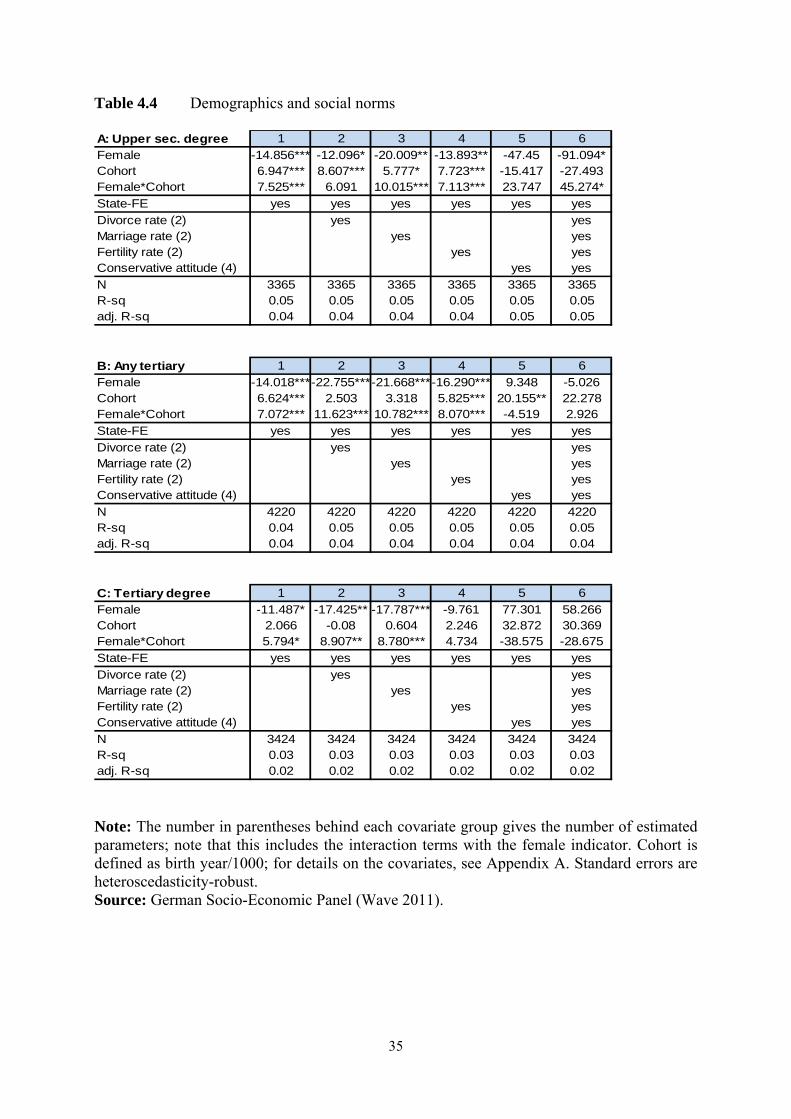
35

Table 4.4 Demographics and social norms A: Upper sec. degree 1 2 3 4 5 6

Female -14.856*** -12.096* -20.009** -13.893** -47.45 -91.094*Cohort 6.947*** 8.607*** 5.777* 7.723*** -15.417 -27.493Female*Cohort 7.525*** 6.091 10.015*** 7.113*** 23.747 45.274*

State-FE yes yes yes yes yes yes

Divorce rate (2) yes yesMarriage rate (2) yes yesFertility rate (2) yes yesConservative attitude (4) yes yes

N 3365 3365 3365 3365 3365 3365R-sq 0.05 0.05 0.05 0.05 0.05 0.05adj. R-sq 0.04 0.04 0.04 0.04 0.05 0.05

B: Any tertiary 1 2 3 4 5 6

Female -14.018***-22.755***-21.668***-16.290*** 9.348 -5.026Cohort 6.624*** 2.503 3.318 5.825*** 20.155** 22.278Female*Cohort 7.072*** 11.623*** 10.782*** 8.070*** -4.519 2.926



N 4220 4220 4220 4220 4220 4220R-sq 0.04 0.05 0.05 0.05 0.05 0.05adj. R-sq 0.04 0.04 0.04 0.04 0.04 0.04

C: Tertiary degree 1 2 3 4 5 6

Female -11.487* -17.425** -17.787*** -9.761 77.301 58.266Cohort 2.066 -0.08 0.604 2.246 32.872 30.369Female*Cohort 5.794* 8.907** 8.780*** 4.734 -38.575 -28.675



N 3424 3424 3424 3424 3424 3424R-sq 0.03 0.03 0.03 0.03 0.03 0.03adj. R-sq 0.02 0.02 0.02 0.02 0.02 0.02 Note: The number in parentheses behind each covariate group gives the number of estimated parameters; note that this includes the interaction terms with the female indicator. Cohort is defined as birth year/1000; for details on the covariates, see Appendix A. Standard errors are heteroscedasticity-robust. Source: German Socio-Economic Panel (Wave 2011).

36

Appendix A: List of control variables and definitions (a) Individual characteristics (SOEP) Secondary degree father & mother - five 0/1 indicators each for Upper secondary degree (reference) Intermediate secondary school degree Lower secondary school degree Other degree or no degree or no schooling Information missing Tertiary degree father & mother - four 0/1 indicators each for Polytechnical or university degree (reference) Vocational training degree No vocational or tertiary education degree Information missing Number siblings - four 0/1 indicators for No siblings (reference) 1-2 siblings 3-20 siblings Information missing Firstborn - three 0/1 indicators for Born first in the sibling row Not born first in the sibling row (reference) Information missing Single parent - number of years spend with a single parent up to age 15 (0-15) 0/1 indicator for information missing Immigrant background father & mother - three 0/1 indicators each for

a. At least one parent is 1rst or 2nd generation immigrant or of non-German b. Not a. (reference)

Information missing Religion - six 0/1 indicators for church affiliation Catholic (reference) Protestant Other christian Other non-christian affiliation No religious affiliation Information missing Religion - five 0/1 indicators for frequency of church attendance Every day or every week (reference) Once a month Not often Never Information missing (b) Labor market characteristics Own sex wage premium: difference in average monthly gross fulltime earnings for age group 20-35 (for

secondary school outcome) and 25-35 (for tertiary outcomes) with vs. without secondary / tertiary degree by sex, state, birth cohort. Forward looking perspective merged for the calendar year in which the observed individual was age 15 / 19. (SOEP)

Other sex wage premium: as above, just use male wage premium in regressions for females and vice versa. (SOEP)

Own fulltime employment premium: difference in average number of years of fulltime employment for age group 20-35 (for secondary school outcome) and 25-35 (for tertiary outcomes) with vs.

37

without secondary / tertiary degree by sex, state, birth cohort. Forward looking perspective merged for the calendar year in which the observed individual was age 15 / 19. (SOEP)

State unemployment rate: state unemployment rate (age 15-64) merged for the calendar year in which the observed individual was age 15 / 19. (Official statistics)

State female LFP: state female share in the labor force (age 15-74) merged for the calendar year in which the observed individual was age 15 / 19. (Official statistics)

Occupational requirement: weighted average of the number of years of education required for occupations in newly started jobs of individuals aged 20-29 in a given calendar year. The average number of years of education by occupation is calculated identically for males and females by calendar year. The weights for the weighted average derive from the relevance of each occupation for the two genders. Variation exists at the sex and year level (not by state). Merged for the calendar year in which the observed individual was age 15 / 19. (SOEP)

(c) Characteristics of the state education system (Official statistics unless stated otherwise) % in upper sec. in grade 7 -

share of pupils in upper secondary education in 7. grade at age 12, by state and year % female upper sec. teachers -

share of females in all upper secondary education teachers at age 12, by state and year % fem. element. teachers -

share of females in all grades 1-4 teachers at age 8, by state and year class size grade 7 upper sec - Average class size grades 7 at upper secondary school at age 12, by state and year class size elementary school - Average class size in grades 1-4 (elementary school) at age 8, by state and year % upper sec. degree at 19 -

share of birth cohort with upper secondary degree at age 19 (three year moving average), by state and year (only for tertiary outcomes in panels B and C) Source: Mikrozensus 2008

(d) Demographics (official statistics) and social norms (Allbus Survey) State FE - ten 0/1 indicators for residence in federal state: Schleswig-Holstein / Hamburg /

Niedersachsen / Bremen / NRW / Hessen / Rheinland-Pfalz / Baden-Württemberg / Bavaria (reference)

Divorce rate - divorces / 10,000 marriages, matched at age 15/19, by state and year Marriage rate - marriages / 10,000 inhabitants, matched at age 15/19, by state and year Fertility rate - births / female population age 18-45, matched 15/19, by state and year Conservative attitude - two measures of

- share of "reference group respondents" (age 18-50, West German residents) who agree or completely agree with the statement "women should stay home and take care of the children" matched at age 15/19, by year - share of "reference group respondents" (age 18-50, West German residents) who agree or completely agree with the statement "after getting married women should leave their job" matched at age 15/19, by year Source: Allbus of 1982, 91, 92, 96, 2000, 04, 08. Missing years were interpolated

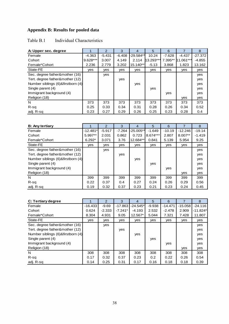
38

Appendix B: Results for pooled data Table B.1 Individual Characteristics A: Upper sec. degree 1 2 3 4 5 6 7 8Female -4.363 -5.431 -6.408 -29.584** 10.24 -7.628 -4.437 -27.372Cohort 9.628*** 3.007 4.149 2.114 13.293*** 7.395** 11.061*** -4.855Female*Cohort 2.236 2.779 3.202 15.140** -5.13 3.868 1.823 13.162



N 373 373 373 373 373 373 373 373R-sq 0.25 0.33 0.34 0.31 0.28 0.26 0.34 0.52adj. R-sq 0.23 0.27 0.29 0.26 0.25 0.23 0.28 0.4

B: Any tertiary 1 2 3 4 5 6 7 8Female -12.481* -5.917 -7.264 -25.005** -1.649 -10.19 -12.246 -19.14Cohort 5.997** 2.031 0.862 0.723 8.674*** 2.807 8.007** -1.419Female*Cohort 6.292* 3.071 3.76 12.684** 0.841 5.139 5.954 9.25



N 399 399 399 399 399 399 399 399R-sq 0.22 0.37 0.4 0.27 0.24 0.26 0.29 0.56adj. R-sq 0.19 0.32 0.37 0.23 0.21 0.23 0.24 0.45

C: Tertiary degree 1 2 3 4 5 6 7 8Female -16.433 -9.69 -17.863 -24.545* -9.938 -14.471 -15.058 -24.116Cohort 0.624 -2.333 -7.241* -4.193 2.532 -2.478 2.909 -11.824*Female*Cohort 8.304 4.931 9.05 12.567* 5.044 7.321 7.428 11.807



N 308 308 308 308 308 308 308 308R-sq 0.17 0.32 0.37 0.23 0.2 0.22 0.26 0.54adj. R-sq 0.14 0.25 0.31 0.17 0.16 0.18 0.18 0.39

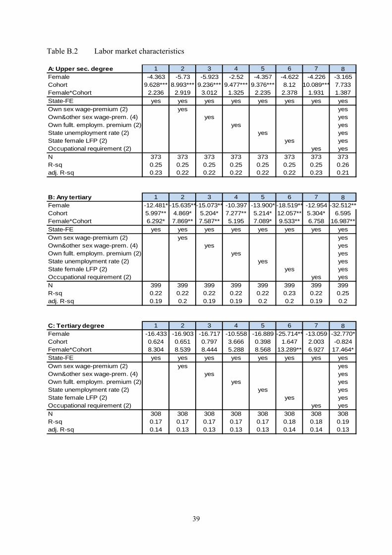
39

Table B.2 Labor market characteristics A: Upper sec. degree 1 2 3 4 5 6 7 8Female -4.363 -5.73 -5.923 -2.52 -4.357 -4.622 -4.226 -3.165Cohort 9.628*** 8.993*** 9.236*** 9.477*** 9.376*** 8.12 10.089*** 7.733Female*Cohort 2.236 2.919 3.012 1.325 2.235 2.378 1.931 1.387



N 373 373 373 373 373 373 373 373R-sq 0.25 0.25 0.25 0.25 0.25 0.25 0.25 0.26adj. R-sq 0.23 0.22 0.22 0.22 0.22 0.22 0.23 0.21

B: Any tertiary 1 2 3 4 5 6 7 8Female -12.481* -15.635**-15.073** -10.397 -13.900* -18.519** -12.954 -32.512**Cohort 5.997** 4.869* 5.204* 7.277** 5.214* 12.057** 5.304* 6.595Female*Cohort 6.292* 7.869** 7.587** 5.195 7.089* 9.533** 6.758 16.987**



N 399 399 399 399 399 399 399 399R-sq 0.22 0.22 0.22 0.22 0.22 0.23 0.22 0.25adj. R-sq 0.19 0.2 0.19 0.19 0.2 0.2 0.19 0.2

C: Tertiary degree 1 2 3 4 5 6 7 8Female -16.433 -16.903 -16.717 -10.558 -16.889 -25.714** -13.059 -32.770*Cohort 0.624 0.651 0.797 3.666 0.398 1.647 2.003 -0.824Female*Cohort 8.304 8.539 8.444 5.288 8.568 13.289** 6.927 17.464*



N 308 308 308 308 308 308 308 308R-sq 0.17 0.17 0.17 0.17 0.17 0.18 0.18 0.19adj. R-sq 0.14 0.13 0.13 0.13 0.13 0.14 0.14 0.13

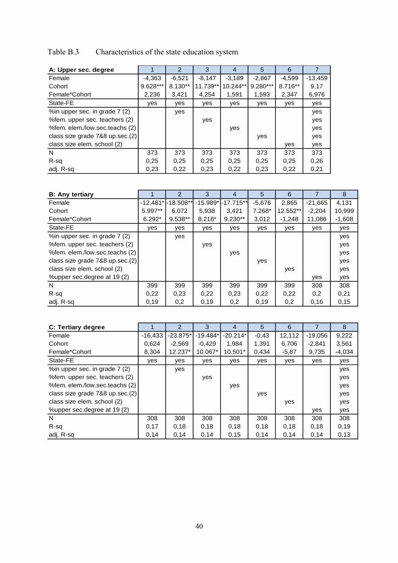
40

Table B.3 Characteristics of the state education system A: Upper sec. degree 1 2 3 4 5 6 7Female -4,363 -6,521 -8,147 -3,189 -2,867 -4,599 -13,459Cohort 9.628*** 8.130** 11.739** 10.244** 9.280*** 8.716** 9,17Female*Cohort 2,236 3,421 4,254 1,591 1,593 2,347 6,976State-FE yes yes yes yes yes yes yes%in upper sec. in grade 7 (2) yes yes%fem. upper sec. teachers (2) yes yes%fem. elem./low.sec.teachs (2) yes yesclass size grade 7&8 up.sec.(2) yes yesclass size elem. school (2) yes yesN 373 373 373 373 373 373 373R-sq 0,25 0,25 0,25 0,25 0,25 0,25 0,26adj. R-sq 0,23 0,22 0,23 0,22 0,23 0,22 0,21

B: Any tertiary 1 2 3 4 5 6 7 8Female -12.481* -18.508** -15.989* -17.715** -5,676 2,865 -21,665 4,131Cohort 5.997** 6,072 5,938 3,421 7.268* 12.552** -2,204 10,999Female*Cohort 6.292* 9.538** 8.218* 9.230** 3,012 -1,248 11,086 -1,608State-FE yes yes yes yes yes yes yes yes%in upper sec. in grade 7 (2) yes yes%fem. upper sec. teachers (2) yes yes%fem. elem./low.sec.teachs (2) yes yesclass size grade 7&8 up.sec.(2) yes yesclass size elem. school (2) yes yes%upper sec.degree at 19 (2) yes yesN 399 399 399 399 399 399 308 308R-sq 0,22 0,23 0,22 0,23 0,22 0,22 0,2 0,21adj. R-sq 0,19 0,2 0,19 0,2 0,19 0,2 0,16 0,15

C: Tertiary degree 1 2 3 4 5 6 7 8Female -16,433 -23.875* -19.484* -20.214* -0,43 12,112 -19,056 9,222Cohort 0,624 -2,569 -0,429 1,984 1,391 6,706 -2,841 3,561Female*Cohort 8,304 12.237* 10.067* 10.501* 0,434 -5,87 9,735 -4,034State-FE yes yes yes yes yes yes yes yes%in upper sec. in grade 7 (2) yes yes%fem. upper sec. teachers (2) yes yes%fem. elem./low.sec.teachs (2) yes yesclass size grade 7&8 up.sec.(2) yes yesclass size elem. school (2) yes yes%upper sec.degree at 19 (2) yes yesN 308 308 308 308 308 308 308 308R-sq 0,17 0,18 0,18 0,18 0,18 0,18 0,18 0,19adj. R-sq 0,14 0,14 0,14 0,15 0,14 0,14 0,14 0,13

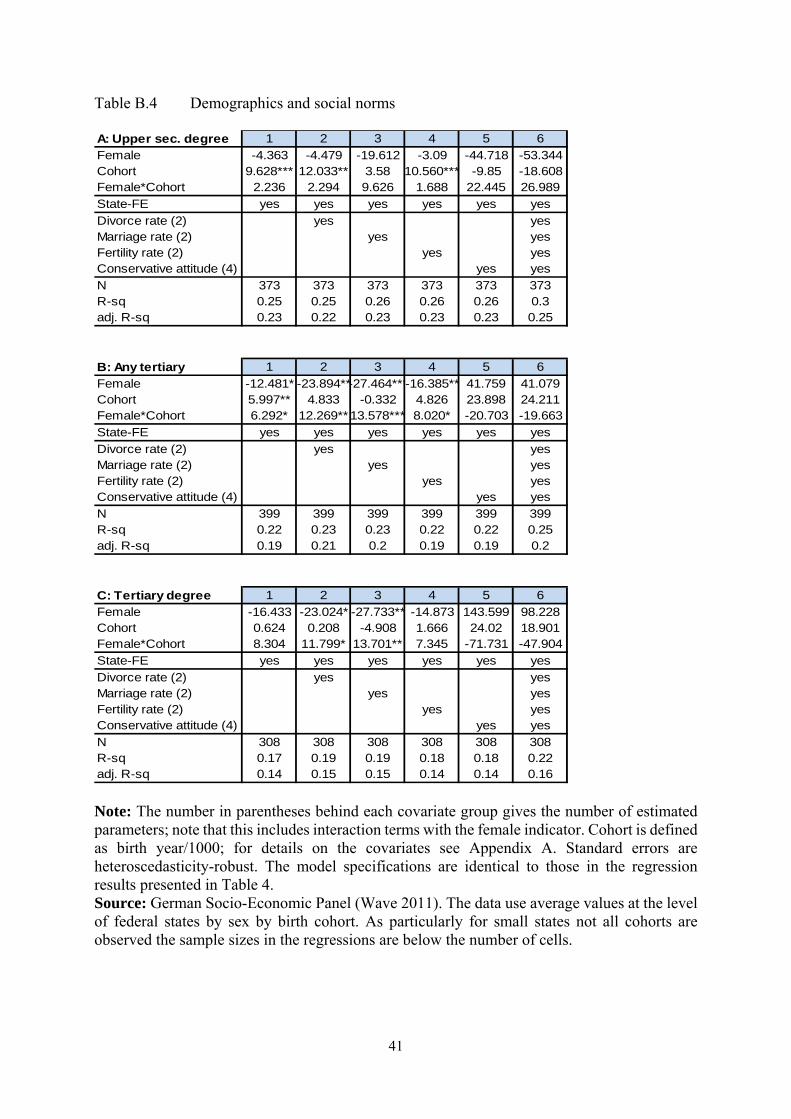
41

Table B.4 Demographics and social norms A: Upper sec. degree 1 2 3 4 5 6

Female -4.363 -4.479 -19.612 -3.09 -44.718 -53.344Cohort 9.628*** 12.033** 3.58 10.560*** -9.85 -18.608Female*Cohort 2.236 2.294 9.626 1.688 22.445 26.989



N 373 373 373 373 373 373R-sq 0.25 0.25 0.26 0.26 0.26 0.3adj. R-sq 0.23 0.22 0.23 0.23 0.23 0.25

B: Any tertiary 1 2 3 4 5 6

Female -12.481* -23.894**-27.464***-16.385** 41.759 41.079Cohort 5.997** 4.833 -0.332 4.826 23.898 24.211Female*Cohort 6.292* 12.269** 13.578*** 8.020* -20.703 -19.663



N 399 399 399 399 399 399R-sq 0.22 0.23 0.23 0.22 0.22 0.25adj. R-sq 0.19 0.21 0.2 0.19 0.19 0.2

C: Tertiary degree 1 2 3 4 5 6

Female -16.433 -23.024* -27.733** -14.873 143.599 98.228Cohort 0.624 0.208 -4.908 1.666 24.02 18.901Female*Cohort 8.304 11.799* 13.701** 7.345 -71.731 -47.904



N 308 308 308 308 308 308R-sq 0.17 0.19 0.19 0.18 0.18 0.22adj. R-sq 0.14 0.15 0.15 0.14 0.14 0.16 Note: The number in parentheses behind each covariate group gives the number of estimated parameters; note that this includes interaction terms with the female indicator. Cohort is defined as birth year/1000; for details on the covariates see Appendix A. Standard errors are heteroscedasticity-robust. The model specifications are identical to those in the regression results presented in Table 4. Source: German Socio-Economic Panel (Wave 2011). The data use average values at the level of federal states by sex by birth cohort. As particularly for small states not all cohorts are observed the sample sizes in the regressions are below the number of cells.

We study the mechanisms that are associated with the … · We study the mechanisms that are...

Documents

Transcript of We study the mechanisms that are associated with the … · We study the mechanisms that are...