WAVE-PROPAGATION SIMULATIONIN AN ELASTIC ANISOTROPIC

(TRANSVERSELY ISOTROPIC) SOLIDBy J. M. CARCIONE.t D. KOSLOFF

(Department of Geophysics and Planetary Sciences, Tel Aviv University, TelAviv, Israel 69978)

and R. KOSLOFF

(Department of Physical Chemistry and The Fritz Haber Research Center forMolecular Dynamics, The Hebrew University, Jerusalem 91904, Israel)

[Received 18 May 1987. Revise 18 September 1987]

SUMMARYA new formulation for wave-propagation simulation in a transversely isotropic

material is presented. A pseudospectral time-integration technique to solve theequation of motion is used, where the propagation is done by a direct expansion ofthe evolution operator by a Chebycheff polynomial series. Examples of wavepropagation in different homogeneous materials and comparison with analyticalsolutions in the symmetry axis, show that the new method is highly accurate. Thepresent numerical simulation can be very important in determining the solution ofelastodynamic problems when the analytical solutions are either very complicated orunknown.

1. Introduction

THE problem of wave propagation through anisotropic solids has beenextensively studied by many researchers (see, for example, Musgrave (1) andPayton (2)), but exact analytical solutions of the wave field are very difficultto obtain, even in the most simple cases. The equations of motion for solidsof low symmetry are extremely complicated. The velocity and wave-frontcurves have only been determinated in detail for hexagonal ^nd cubicmaterials. The simplest is the hexagonal system which belongs to the class oftransversely isotropic solids, due to the circular symmetry around thehexagonal axis. For this type of anisotropy exact analytical solutions of thewave field have been calculated for homogeneous media only along thesymmetry axis (3), and for the surface wave-motion problem of a point-loaded half-space (4) (Lamb's problem).

As mentioned before the type of transversely isotropic materials includeshexagonal crystals and also may be a very good representation of the earth'sstructure. The real earth is generally stratified with elastic properties anddensity which vary stepwise with increasing depth. If the dominant

tOn leave from: Yacunientos Petroliferos Fiscales, Gerencia de Exploration, Pte. R. S.Pena 777, 1364 Buenos Aires, Argentina. Present Address: Hamburg University, D-2000Hamburg, Federal Republic of Germany.

[Q. Jl Meed. ippL Math., Vol. 41, Pi. 3, 1988] © Oxford Unlrcnitjr Prco 19S8

320 J. M. CARCIONE ET AL.

wavelength of the wave field is long enough compared to the dimensions ofthese varying strata, an averaging effect takes place which leads totransverse isotropy. In the first case measurements of ultrasonic wavepropagation are performed in order to determine the elasticities of crystals,and in the latter case information about the lithology of formations isextracted through the inversion of the seismograms.

Wave-propagation simulation has been advancing considerably in recentyears (see, for example, Aboudi (5)). With the progress in new methods andnew computer technology, it has become possible to solve the governingwave equation with a high degree of precision. This combined withsignificant advances in data quality suggests a strong need to develop anaccurate algorithm for wave-propagation calculations in anisotropic media.

This paper considers two-dimensional wave propagation through a generalheterogeneous transversely isotropic medium. To solve the equation ofmotion, a new time-integration technique is used. The method is veryaccurate and yet involves the same amount of computational effort assecond-order finite differences in time. This new pseudospectral numericalscheme (6) has already been successfully applied to solving the acoustic (7)and SchrOdinger (8) wave equations, and to the viscoacoustic (9) andviscoelastic (10) equations of motion.

The first section presents the constitutive relation of the transverselyisotropic solid. Then the equation of motion for the two-dimensional case isderived, and the numerical algorithm is developed. The next section reviewssome basic concepts about the velocity and wave-front curves in transverselyisotropic materials, and finally examples of wave propagation are presented.

The numerical algorithm is tested against the problem of wave propaga-tion in a homogeneous class IV transversely isotropic media.

2. Constitutive relations of the transversely isotropic mediumThe constitutive relation of a heterogeneous anisotropic and elastic solid

is expressed by the generalized Hooke's law, which can be written as

Oij = cijkleu, i, j , k, I = 1,... , 3, (2.1)

where t is the time, x is the position vector, a,y(x, t) and %(x, t) are theCartesian components of the stress and strain tensors respectively, andCjjU(x) are the components of a fourth-order tensor called the elasticities ofthe medium. The Einstein convention for repeated indices is used.

To express the stress-strain relation for a transversely isotropic mediumwe introduce a shortened matrix notation commonly used in the literature.With this convention, pairs of subscripts concerning the elasticities arereplaced by a single number according to the following correspondence:

(11)->1, (22)->2, (33)-* 3, (23) = ( 3 2 ) - 4 ,

(31) = (13)-* 5, (12) = (21)-* 6.

SIMULATED ELASTIC-WAVE PROPAGATION 321

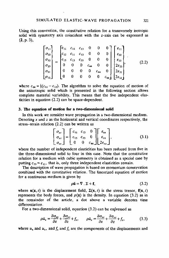
Using this convention, the constitutive relation for a transversely isotropicsolid with symmetry axis coincident with the z-axis can be expressed as(2, p. 3),

31

;11

:12

:13

000

Cl2

Cll

Cl3

000

Cl3

Cl3

C33

000

000

C44

00

0000

C44

0

0

0

0

0

0

c«,

£22

£33

2e31

(2.2)

where cM = \{cn — c12). The algorithm to solve the equation of motion ofthe anisotropic solid which is presented in the following section allowscomplete material variability. This means that the five independent elas-ticities in equation (2.2) can be space-dependent.

3. The equation of motion for a two-dimensional solidIn this work we consider wave propagation in a two-dimensional medium.

Denoting x and z as the horizontal and vertical coordinates respectively, thestress-strain relation (2.2) can be written as

Ozz

Cll

Cl3

0

Cl3

C33

0

0 "0

C 4 4 _

Exx

Mxz.

(3.1)

where the number of independent elasticities has been reduced from five inthe three-dimensional solid to four in this case. Note that the constitutiverelation for a medium with cubic symmetry is obtained as a special case byputting c33 = cn, that is, only three independent elasticities remain.

The description of wave propagation is based on momentum conservationcombined with the constitutive relation. The linearized equation of motionfor a continuous medium is given by

pu = V . 2 + f, (3.2)

where u(x, t) is the displacement field, 2(x, t) is the stress tensor, f(x, t)represents the body forces, and p(x) is the density. In equation (3.2) as inthe remainder of the article, a dot above a variable denotes timedifferentiation.

For a two-dimensional solid, equation (3.2) can be expressed as

dx dzpuz =

do^

dx dz(3.3)

where ux and uz, zndfx and/j are the components of the displacements and

322 J. M. CARCIONE ET AL.

body forces respectively. By replacing the constitutive relation (3.1) in theequations of motion (3.3), and making use of the strain-displacementrelations (11, p. 13), we obtain

3

3

3

(3.4)

The equations of motion for an isotropic solid are a special case ofequations (3.4) when cn = c33 = k + 2fi, cu = A, and c^ = /z, where X and pare the Lame" constants.

4. Numerical algorithmIn order to solve the problem numerically we recast equations (3.4) as a

coupled first-order equation in time as follows:

U = MU + F, (4.1)

where M is a spatial operator matrix of dimension 4 given by

" 0 0 1 0 "0 0 0 1

M31 A/32 0 0M42 0 0 .

M =

with its components denned by

i / aM

(4.2)

l / a dd d\32 = - I — C 1 3 — + — C 4 4 — ,

p \dx dz dz dx)1/3 3 3 3\

*41 = - I — C44 — + — C13 — ,

p\3x 3z dz 3x)1 13 3 3 3p \3x dx dz dz

(4.3)

and

with the source vector,

U r = [ux, uz, ux, uz],

FT = [0,O,/x/p,/ r/p].

(4.4)

(4.5)

After a spatial discretization in x and 2 and a suitable approximation for thespatial derivatives, equation (4.1) becomes a coupled system of

SIMULATED ELASTIC-WAVE PROPAGATION 323

4N^4NZNZ ordinary differential equations in the unknowns ux, uz, ux anduz at the grid points. The numbers of grid points in the x- and z-directionsare denoted by Nx and Nz respectively.

In this work we calculate the spatial-derivative terms by the Fourierpseudospectral method (12,13), which consists of a spatial discretizationand calculation of spatial derivatives using the fast Fourier transform (FFT).For instance, the quantity (3/3x)c1 3(3u I /3z) in equation (3.4)x is calculatedin the following way. First, along each z-line a spatial FFT on uz isperformed. The result is then multiplied by the complex spatial-wave-number vector,

UCv= ^ N ^ NNDZ' V = ^N"->^N"

where DZ is the grid spacing in the z-direction and i2 = —1. This operationis followed by an inverse FFT into the spatial domain yielding duz/dz,which is then multiplied by c i 3 . Then forward and inverse FFTs along eachx-line are performed to calculate (9/dx)cl3(duz/dz).

Equation (4.1) can be expressed in compact notation as

UA, = MAfUiV + FA,, (4.6)

subject to the initial conditions

U*(0) = US,, (4.7)

where I V , M^ and ¥N are the discrete representations of U, M and Frespectively. The solution to equation (4.6) subject to (4.7) is formally givenby

[ eM»zVN(t -+ [ eM»zVN(t - T) dx. (4.8)

We consider a separable source term ¥N(t) = \Nh(t), where AN is thespatial distribution of the source, usually chosen to be a delta or a highlylocalized function. The function h(t) is the source-time history. Consideringzero initial condition and replacing the source term, equation (4.8) becomes

VN = [fe^hit - T) dx^\N. (4.9)

To solve this equation we use a new time-integration technique based on thewell-known Chebycheff expansion of the function ez (6),

l , (4.10)

where \z\ =£ zR and z lies close to the imaginary axis. Now Co = 1 and Ck = 2for k 5s 1, Jk is the Bessel function of order k and Qk are the modified

324 J. M. CARCIONE ET AL.

Chebycheff polynomials which satisfy the recurrence relation

Qk+1(s) = 2sQk(s) + Qk-!(s), (4.11)

withCo = l and £>!=.$. (4.12)

Substituting T M ^ for z in (4.10), equation (4.9) becomes

VN(t) ~ U* = £ Ckbk(tR)Qk\y*]AN, (4.13)

where the coefficients fct are given by

bk=fjk(zR)h(t-r)dT. (4.14)Jo

The variable R must be chosen larger than the region spanned by theeigenvalues of MN, which should be in the vicinity of the imaginary axis(this is shown in Appendix A together with the determination of R).Tal-Ezer (6) showed that the largest k = K in equation (4.13) should begreater than tR to ensure convergence. The actual value of K can bedetermined by finding the range in which the coefficients bk are significantlydifferent from zero.

The starting values for the recursion are given by

QO[^]AN = AN and Q ^ A ^ ^ A * , (4.15)

according to equation (4.12). Additional terms are generated by (4.11) withMN/R replacing s, while U£ is cumulated by (4.13). The final value of U£ isobtained after cumulating K terms.

The solution can be propagated in time again by considering U%(t0) as aninitial condition, by means of the homogeneous solution in equation (4.8).This yields

VN(t) - U£ = f CkJk{tR)QJ^Wa (4.16)= 0

where tQ is the size of the first time increment which should be larger thanthe duration of the source time history. The calculation of time histories at agiven point of the material does not require significant additional computa-tional effort since the terms Qk(MN/R)UN are calculated in any case; onlyadditional sets of Bessel functions need to be generated. The intermediateresults are calculated according to

VN(t') ~ U£ = £ CkJk{fR)QJ^Wo) (4.17)*-o L K J

for t' < t.

SIMULATED ELASTIC-WAVE PROPAGATION 325

Because the Fourier pseudospectral method considers the discretizedvariables on the grid as periodic functions, absorbing boundaries areimplemented to prevent wrap-around, the phenomenon in which a pulsewhich leaves the grid on one side re-enters it on the opposite side. Toeliminate this effect from the boundaries of the numerical grid, we use amethod developed by Kosloff and Kosloff (14). The absorbing boundary isperformed through a systematic elimination of the wave amplitude in a stripalong the boundary of the grid. This is achieved by replacing the operator Min equation (4.1) by the operator (M — al), where I is the identity matrixand a, which determines the absorption, is given by

a =UQ/cosh2 (6m), (4.18)

where C/o is a constant and 6 is a decay factor. The parameter a(x, z) ischosen in order that it differs from zero only in a strip of nodes (m)surrounding the numerical mesh.

Equation (4.18) has the functional form of the complex potentials used inquantum mechanics, where with an appropriate choice of the parameters itis possible to eliminate reflected or transmitted energy from the absorbingregion. The spatial dependence of a(x, z) is chosen to give the bestamplitude elimination.

To clarify the method we consider the one-dimensional version ofequation (4.1) with constant material properties and zero source term,

1? -" [";]•where c is the wave velocity. When a = 0, the first equation in (4.19)expresses the relation V = dujdt, whereas the second one is the acousticwave equation. With the inclusion of the parameter a and eliminating thevariable V, equation (4.19) reads

y - 2auz - o?ux. (4.20)dx

This equation has a general solution of the form

ux(x, t) = Afr(x - ct)e-(°"c)z + Bf2{x + c^"1^, (4.21)

with A and B arbitrary constants and fx and f2 arbitrary twice-differentiablefunctions. The solution represents attenuating waves in space, where allfrequency components are equally attenuated. This means that the absorb-ing boundary will gradually attenuate the wave field without changing its shapeor producing dispersion.

326 J. M. CARCIONE ET AL.

5. The velocity and wave-firont corves in a homogeneous medinni

The normal curve for a transversely isotropic solid is defined by thefollowing parametric form (2, p. 17):

p = R±(6) cos 0 and q = R±(6) sin 0, (5.1)

where

2MB)with

_R±(6) - I 2MB) J

} (5-3)A(d) = a cos" 0 + y cos2 0 sin2 0 + 0 sin4 0,

5(0) = (a- +1) cos2 0 + 03 + 1) sin2 0.

The parameters a, /3 and y in equations (5.3) are given by

The velocity curve is the inverse of the normal curve and is definedparametrically by

vx± = V±(6)sind and vz± = V±(0) cos 0, (5.5)

with

V±(6) = Vs/R±(d), (5.6)

and

(5.7)

is a reference wave velocity of the medium, which in a transversely isotropicmedium corresponds to the vertical and to the horizontal pure transversewave velocity (15).

The velocity curve consists of two branches differentiated by the sign in(5.5). Under the condition of strict hyperbolicity (2, p. 18) we must have

V+(0) < V.ifi). (5.8)

The velocity curve defined by the minus sign in (5.5) corresponds to thequasilongitudinal mode, and that defined by the plus sign to the quasi-transverse mode. The displacement amplitudes corresponding to thesemodes are always orthogonal, but not perpendicular or coincident with thewave front as in the isotropic solid. In seismology these modes represent theP and SV wave fronts, but actually the waves are purely compressionalor shear only when the direction of propagation is perpendicular to(VP= (cn/p)i), or coincident with (VP = (c33/pp) the symmetry axis of thetransversely isotropic solid (15).

The wave-front curve, which is constructed as the envelope of planewaves at a given time t, consists also of two branches defined parametrically

SIMULATED ELASTIC-WAVE PROPAGATION 327

by (2, p. 35),

V± /cos0r 2a . 2a sin2Ofacos2 6 - k2sin2 6)Z± = ' 1A

" v~ ""' " \ (5 9)V±tsind[ O . 2n 2n cos20(A:1cos20-A:2sin20)- '

x+ =——— 2psin 0 + ycos 0 T j—^— i2/4. L (B ~ 4/l)i

where fc, = 2or(/3 + 1) + y(ar + 1) and )k2 = 2/3(o- + 1) - y()3 + 1).The normal and wave-front curves in transversely isotropic materials are

classified according to the existence and location of inflexion points andcusps respectively (2, pp. 26, 38). The existence of inflexion points in thenormal curve gives rise to lacunae or cusps in the wave-front curve.

It is important to point out that there is no simple correspondencebetween the velocity and wave-front curves. The velocity V±(d) measuresthe velocity of advance of the wave front along the wave-number vectork(0), which is normal to the wave-front curve. Given a point P = (x0, ZQ) onthis curve, the corresponding point Q = (vZo, v^ is obtained by passingthrough the origin a line parallel to the direction of the vector k andintersecting the velocity curve (15). Only for spherical wave fronts (isotropiccase) will the points P and Q lie on the same radial line.

6. Wave-propagation simulationNow we examine wave propagation through different materials (homoge-

neous and heterogeneous), and test the numerical algorithm against theanalytical solution along the symmetry axis.

6.1 Wave fronts in three different hexagonal crystalsThe motion is initiated by a z-directional point force located at the centre

of a 165 X 165 grid with spacing DX = DZ = 0-2 cm. The source is a shiftedzero-phase pulse defined by

F(t) = e-°-5^-^ cos nfo(t- t0), (6.1)

with to = 6fis and a high cut-off frequency f0 = 5 x 10s Hz. No absorbingboundaries are used in this case because the perturbation does not exceedthe grid limits.

Table 1 shows the elasticity constants and densities of the three materials.The last column presents the time at which the snapshots are calculated.The materials are classified according to the existence and location ofinflexion points in the normal curve or, equivalently, of cusps in thewave-front curve.

Figures 1 and 2, and 3 and 4 show the velocity curves, wave-front curvesand snapshots of the three crystals, respectively (a) for apatite, (b) for zinc,and (c) for cobalt. Figures 3 represent the ux-components of the wave front

328 J. M. CARCIONE ET AL.

TABLE 1. Material properties of the hexagonal crystals

Density Timeci3 c33 c« (grcm"') (us)Crystal Oass c,

ApatiteZincCobalt

IVIVV

16-716-530-7

6-650

10-3

14-06-2

35-8

6-633-967-55

3-2718-9

203224

The elasticities should be multiplied by 10u dyne cm"

and Figs 4, the uz-components. The velocity and wave-front curves have thecorresponding inflexion points and cusps, respectively, according to theclassification given by Payton (2, pp. 26, 38). The cuspidal triangles aroundz+ = 0 in zinc cannot be seen because they are too small.

All the wave fronts show the characteristics predicted by the respectivewave-front curves, with the quasilongitudinal mode weaker than thequasitransverse mode. It can be seen also that the ux-component along thesymmetry axis is zero, in agreement with the theoretical solution given byequation (B.3).

Due to symmetry considerations, the ux wave fronts should show

FIG. 1. Velocity curves for (a) apatite, (b) zinc, and (c) cobalt. The minussign corresponds to the quasilongitudinal mode, and the plus sign to the

quasitransverse mode

SIMULATED ELASTIC-WAVE PROPAGATION 329

- 8 - 6 - 4 - 2 0

- 8 - 6 - 4 - 2 0 2 4 6K<t (km s-1)

FIG. 1. (Continued)

330 J. M. CARCIONE ET AL.

-16 -12 - 8 - 4 0

-12

-16-16

FIG. 2. Wave-front curves for (a) apatite, (b) zinc, and (c) cobalt. Theminus sign corresponds to the quasilongitudinal mode, and the plus sign to

the quasitransverse mode

SIMULATED ELASTIC-WAVE PROPAGATION 331

12 16

FIG. 2. (Continued)

antisymmetric behaviour across x = 0 and z = 0, and the uz wave frontsshow symmetric behaviour across the same lines. The effects can bevisualized for both components across z = 0, but because of the nature ofthe display, these are not evident across x = 0. A careful analysis revealsthat equidistant points at both sides of the line x = 0 for the ux wave frontshave the same amplitude but opposite sign (antisymmetry). The sameanalysis shows that the uz wave fronts are symmetric across x = 0.

6.2 Wave propagation in a heterogeneous materialThis example considers wave propagation in a region consisting of two

materials (Fig. 5). The left half-space is zinc and the right half-space is anisotropic solid with the following properties:

c n = 16-5, c33 = 16-5, c,3 = 8-58, 044 = 3-%, p = 7-lgrcm"3,

where the elasticities should be multiplied by 1011 dyne cm"2. This solid canbe considered as an isotropic zinc, because the compressional and shear-wave velocities corresponds to the pure longitudinal (horizontal direction)and pure transverse wave velocities in zinc.

The simulation uses the grid parameters and pulse function of theprevious example, but the source position is shifted from the centre of the

332 J. M. CARCIONE ET AL.

16

12

12 16

i) x (cm)

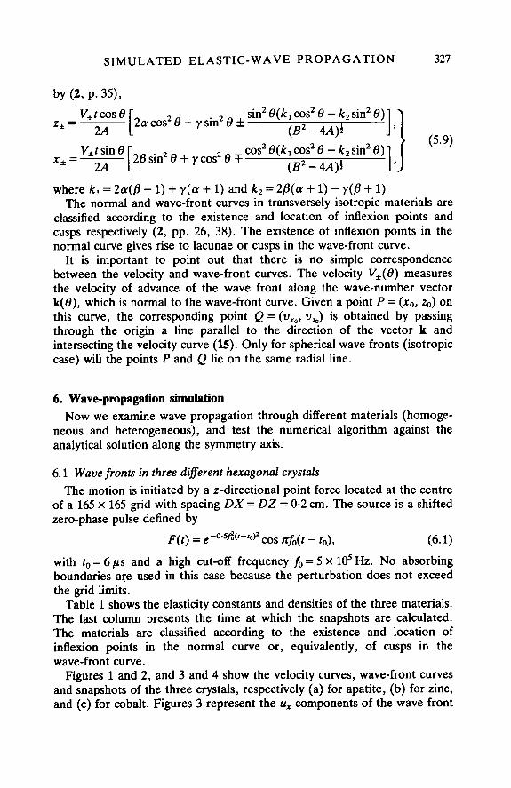
FIG. 3. ^-components of the wave front for (a) apatite, (b) zinc, and (c)cobalt, due to a z-directional point force

grid (it is indicated by S in Fig. 5b). Snapshots of the wave field at t = 32 fxsafter the excitation of the source are shown in Figs 5a (ux-component) and5b (uz-component). The main wave fronts present the expected characteris-tics of zinc (see Figs 3b and 4b) in the left half-space, and of an isotropicsolid (concentric circles) in the right half-space.

A detailed interpretation of the snapshots allows the identification of thefollowing events.

(A) Primary quasilongirudinal wave.(B) Primary quasitransverse wave.(C) Reflected quasitransverse wave.(D) Converted quasitransverse wave generated by reflection of A.(E) Head wave which connects A with the transmitted longitudinal wave

H.

SIMULATED ELASTIC-WAVE PROPAGATION 333

£ 0

- 4 -

- 8 -

- 1 2 -

- 1 6

-

(b)

16 - 1 2 - 8

FIG.

—

3

4 0

v (cm)

. (Continued)

(F) Reflected quasilongitudinal wave.(G) Converted quasilongitudinal wave generated by reflection of B.(H) Transmitted longitudinal wave.(I) Transmitted transverse wave.(J) Transmitted transverse wave generated by the cusps.

(K) Converted transverse wave generated by transmission of A.The application shows how the model can handle the large number of

phenomena present in heterogeneous materials, even the small-amplitudehead-wave fronts.

6.3 Comparison with analytical resultsIn class IV transversely isotropic media the wave-front curve has four

cuspidal triangles, two centred on the z+-axis, and two centred on the

334 J. M. CARCIONE ET AL.

- 1 2 -

- 1 6 -

- 1 6

(c)

-12 - 8 - 4 0

x (cm)

Fio. 3. (Continued)

16

x+-axis. In the apatite, as can be seen from Fig. 2a, a line drawn very closeto the axis of symmetry, for example, intersects the wave-front curve in fourpoints. This means that a single pulse at the origin will produce fourseparated pulses of energy.

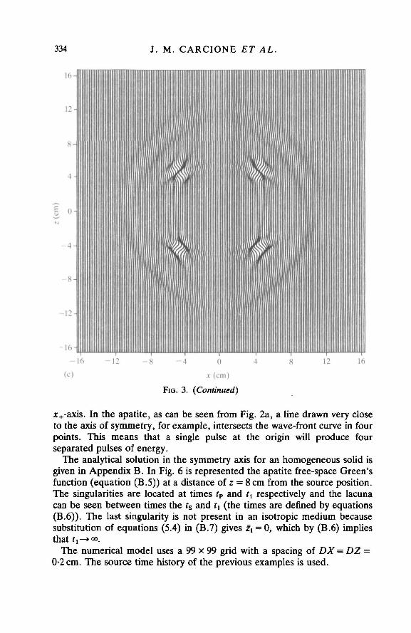
The analytical solution in the symmetry axis for an homogeneous solid isgiven in Appendix B. In Fig. 6 is represented the apatite free-space Green'sfunction (equation (B.5)) at a distance of z = 8 cm from the source position.The singularities are located at times tP and tx respectively and the lacunacan be seen between times the ts and tx (the times are denned by equations(B.6)). The last singularity is not present in an isotropic medium becausesubstitution of equations (5.4) in (B.7) gives zx = 0, which by (B.6) impliesthat *!-»<».

The numerical model uses a 99 x 99 grid with a spacing of DX = DZ =0-2 cm. The source time history of the previous examples is used.

SIMULATED ELASTIC-WAVE PROPAGATION 335

16-

12

16

Fia. 4. M,-components of the wave front for (a) apatite, (b) zinc, and (c)cobalt, due to a z-directional point force

Figures 7a and 7b compare numerical and analytical solutions at distancesof 2-6 and 8 cm from the source position respectively. As the figures show,the comparison between numerical and analytical solutions is excellent.

7. Conclusions

This work has dealt with wave-propagation simulation in a two-dimensional transversely isotropic solid. The equations of motion are solvedusing a new pseudospectral numerical scheme in time. The method is basedon the approach introduced by Tal-Ezer (6), in which the evolutionoperator is expanded in a Chebycheff polynomial series. Wave frontscalculated by the simulation algorithm show the characteristics predicted bythe respective wave-front curves. The theory has been tested successfully

336 J. M. CARCIONE ET AL.

16

P 0

- 4

- 8

•12

- 16

- 16

(b)

- 12 - 4 (I 4

x (cm)

FIG. 4. (Continued)

12 16

SIMULATED ELASTIC-WAVE PROPAGATION 337

16

16

FIG. 4. (Continued)

338 J. M. CARCIONE ET AL.

- 1 6 - 1 2

(a)

- 8 - 4 0

x (cm)

12

8-

4 -

(1-

- 4 - 1

— 8-

12-

- 1 6 -

1A l

HHillli111in•i

1iUuffiiUH H

^ ^ " ^ i i f f l P i i i l f l i^ f f iWi i '

^SiffiiffiMill HlIlillllWlllfflllflfllMllllmffililllllllllllr

l l l l l l i l l l l l i l l i i l l l l l i l l l l l i l l l l l^

1 116

FIG. 5. Snapshots at f = 32/*s for a heterogeneous material composed ofzinc (left half-space) and an isotropic solid (right half-space); (a) ux-

component, (b) uz-component

SIMULATED ELASTIC-WAVE PROPAGATION 339

16

Fio. 5. (Continued)

340 J. M. CARCIONE ET AL.

10

0-5

-0 -5

- 1 0

+ 00 1

'/

+ 00 1

/

V

10 20 30 40 50

Time (/is)

FIG. 6. Free-space Green's function (uzz(x, t)) due to a z-directional pointforce versus time in apatite, at a distance of 8 cm from the source position

10

0-5

E

-0 -5

- 1 0

(a)NumericalAnalytical

10 20 30Time (fis)

40 50

Time (jis)

FIG. 7. Time-history comparison between the numerical and analyticalsolutions in the symmetry axis (time convolution of uXI(t) with F(t)) atdistances of (a) 2-6 cm and (b) 8 cm from the source position, due to a

z-directional point force. The medium is apatite

342 J. M. CARCIONE ET AL.

also when the medium is heterogeneous. The accuracy of the algorithm wasverified in the comparison with the analytical solution in the symmetry axisof the material. The present numerical simulation can be very important indetermining the solution of elastodynamic problems when the analyticalsolutions are either very complicated or unknown. Possible applicationsinclude realistic simulation of wave propagation through the earth, as wellas in the field of material science. Extension of the algorithm to problemsinvolving wave propagation in materials of different symmetry will becarried out in a future work.

Acknowledgement

This work was partially supported by a research project on three-dimensional seismic modelling conducted jointly between the University ofHamburg and Tel Aviv University under contract 03E-6424-A of theBMFT, Federal Republic of Germany, and contract EN3C-0008-D of theEuropean Community Commission.

REFERENCES1. M. J. P. MUSGRAVE, Crystal Acoustics (Holden-Day, San Francisco 1970).2. R. G. PAYTON, Elastic Wave Propagation in Transversely Isotropic Media

(Martinus Nijhoff, The Hague 1983).3. R. G. PAYTON, Z. angew. Math. Phys. 29 (1978) 262-272.4. R. BURRIDGE, Q. Jl Mech. appl. Math. 24 (1971) 81-98.5. J. ABOUDI, Modern Problems in Elastic Wave Propagation (eds J. Miklowitz

and J. D. Achenbach; Wiley, New York 1977) 45-65.6. H. TAL-EZER, S1AM J. numcr. Anal. 23 (1986) 11-26.7. , D. KOSLOFF and Z. KOREN, Geophys. Prosp. 35 479-490.8. and R. KOSLOFF, J. Chem. Phys. 81 (1984) 3967-3971.9. J. M. CARCIONE, D. KOSLOFF and R. KOSLOFF, unpublished.

10. , and , unpublished.11. K. AKI and P. G. RICHARDS, Quantitative Seismology, Theory and Methods

(Freeman, San Francisco 1980).12. B. FORNBERG, SIAM J. numer. Anal. 12 (1975) 509-528.13. D. KOSLOFF and E. BAYSAL, Geophysics 47 (1982) 1402-1412.14. and R. KOSLOFF, J. Comp. Phys. 63 (1986) 363-376.15. G. W. POSTMA, Geophysics 20 (1955) 780-806.

APPENDIX AEigenvalues of the propagation matrix and determination of R

A plane-wave solution to equation (4.1) is assumed of the form

V = Voe'ia'-^\ (A.I)

where a) is the angular frequency, k is the wave-number vector given by k = (kx, kx),and x is the position vector. Considering constant elasticities and density and a zero

SIMULATED ELASTIC-WAVE PROPAGATION 343

source term, substitution of (A.I) in equation (4.1) yields

" 0 0 1 0 "0 0 0 1

M31 Mx 0 0M41 Mn 0 0

U, (A.2)

where the spatial double Fourier transform of the components of M are given byL _ K2

(c13 + cM)kxkz (A.3)

Equation (A.2) forms an eigenvalue equation for the eigenvalues A, = ico, i = 1.....4.The characteristic equation of (A.2) is given by

A? - (M3 1 = 0. (A.4)

For a transversely isotropic solid the constraints on the elasticities are as follows:Cii,c33ic«>0; \c^ + cu\<[(cncyi)

}i + c»] (2, p. 11). Thus B = -(Af3I + A£«)>0,Co(M31M«-M ( lM32)>fl and B 2 - 4 C > 0 . With these conditions the roots ofequation (A.4) lie on the imaginary axis. The eigenvalues are

*>i + Mn\ - [(M31 - \U2

For an isotropic solid, equations (A.3) become

A2 = -A,,

A4=-A3.(A.5)

= "*41 ^

P

(A.6)

Substitution of these expressions in equations (A.5) yields

(A.7)

The first and second eigenvalues correspond to longitudinal wave propagation, andthe third and fourth to shear wave propagation. They define the dispersion relations

and w = vs(k2

x (A.8)

344 J. M. CARCIONE ET AL.

for longitudinal and shear waves respectively, where vP = ((A + 2/i)/p)i, andf s f

Similarly, for a transversely isotropic solid, A, = ica and A3 = i(o define thedispersion relations. Note that substitution of the parametric form

kx=k(d) sin 6, kL = k(d) cos 0 (A.9)

in the dispersion relations yields k±(0) = co/V±(6), where V±(0) is the phasevelocity (5.6). A numerical evaluation of the dispersion relations reveals thatW ) l = V-(6) (quasilongitudinal mode), and |A3(0)| = V+(8) (quasitransversemode). This can also be deduced from the isotropic limit, equations (A.7).

The range of the eigenvalues of the propagation matrix, R, is obtained bysubstitution of k% = n/DX and A^ = n/DZ (the Nyquist wave numbers give thehighest eigenvalues) in equations (A.5). For the isotropic case we obtain

( A 1 0 )

using the fact that vP > vs, while for a transversely isotropic solid, R is given by

R = IW, O, (A.ii)where the condition of strict hyperbolicity (5.8) was used. In the heterogeneouscase, the elasticities which give t ie maximum R should be chosen.

APPENDIX BFree-space Green's function along the symmetry axis for the transversely isotropicsolid

The two-dimensional anisotropic Green's function u^ix, t) satisfies the followingequation of motion:

= P Hi*' '"';"' k>l'p = h 2' (B1)

where /^ is the impulsive body force given by

/„ = 8lp8(x)6(z)d(t). (B.2)

Denning the dimensionless variable

Z=Z/T,

with

T=Vst,

where Vs is given by equation (5.7), the solution to equation (B.I) for class IVtransversely isotropic materials along the symmetry axis z is (2, p. 78)

(B.3)

t>tu

SIMULATED ELASTIC-WAVE PROPAGATION 345

with

m ) h [&(frF? ] [ { y 0 ) >^( f f ^o ^ r *.and

tf<t<ts,r s « /« / l f (B-5)

with1 r i 2(1 - f2) - {y - (ft + l)f2} If - {y - tf + l)z2} + Dhh

l(2)~^rU Wl JL -2(a--z2)(l-f2) J '

where

ts = z/(cjp)i, <p = z/(c33/p)i, f, = fs/z,. (B.6)

The quantity D(f) is given by

and

+ 1) - 2/5(ar + 1) + 2{P(1 + «{}- y)(cr + /S - y)}i]i/(/S - 1). (B.7)

To perform the comparison with the numerical solution we convolve the free-spaceGreen's function with the shifted zero-phase pulse function given by (6.1).