Water Use Conflicts in East Africa - University of Rhode ...
75
Water Use Conflicts in East Africa Irrigation demand of a biofuel crop in the Wami Basin, Tanzania Eivy Y. Monroy A RESEARCH PROJECT SUBMITTED IN PARTIAL FULFILLMENT OF THE REQUIREMENTS FOR THE DEGREE OF MASTER OF ENVIRONMENTAL SCIENCE AND MANAGEMENT UNIVERSITY OF RHODE ISLAND 2010
Transcript of Water Use Conflicts in East Africa - University of Rhode ...

Water Use Conflicts in East
Africa Irrigation demand of a biofuel crop in the Wami
Basin, Tanzania
Eivy Y. Monroy
A RESEARCH PROJECT SUBMITTED IN PARTIAL FULFILLMENT OF THE REQUIREMENTS
FOR THE DEGREE OF MASTER OF ENVIRONMENTAL SCIENCE AND MANAGEMENT
UNIVERSITY OF RHODE ISLAND
2010

Abstract
The demand for water exceeds available supplies in many watersheds of East Africa. The Wami
River system, one of the most important watersheds in Tanzania for agro-industry and
biodiversity, follows this trend. The Wami River flows through Saadani National Park in the
coastal basin, with the Indian Ocean its final destination. A project proposal to develop biofuel
from sugarcane (Saccarum officinarum) in the lower Wami watershed would draw water from
the Wami for irrigation. Sugarcane is a high biomass crop that requires large quantities of water
(approximately 1500-2000 mm over the growing season) from both rainfall and irrigation, for
maximum production of sucrose, which can be converted into ethanol. The objectives of this
paper are to estimate irrigation demands of 15,000 ha of planted sugarcane under different
irrigation regimes and water stress during the growing season. A model of the Food and
Agriculture Organization of United Nations (FAO) named Aquacrop is used for this purpose.
The outputs are compared with historic seasonal flows of the Wami River. Aquacrop is a robust
water-driven crop model that simulates yield response to water use based on sugarcane growth
parameters and inputs of climatic data, crop characteristics, soil, and management characteristics
that together define the environment in which the crop will develop. Aquacrop was introduced in
2009, and is widely used in African countries. The final goals of this research are to estimate
crop requirements for assessing the impact of the proposed biofuel production on Wami River
flows near the National Park and to contribute to improved water supply management.
Predictions of irrigation supply for growing 15,000 ha of sugarcane in Razaba Ranch using
AquaCrop as a water-drive model, estimate that water withdrawal from the Wami River will
exceed the water available for maintaining the seasonal flows.
Table of Contents
1. Introduction ................................................................................................................................1
2. Problem Statement.....................................................................................................................1
3. Objectives....................................................................................................................................3
4. Lower Wami River and Its Flows.............................................................................................4
4.1 Ecological functions ...............................................................................................................9
4.1.1 Wildlife ............................................................................................................................9
4.1.2 Surrounding habitats ......................................................................................................10
4.1.3 Fisheries .........................................................................................................................11
4.1.4 National Park sustainability ...........................................................................................11
4.1.5 Livelihoods ....................................................................................................................12
5. Biofuel Project Background ....................................................................................................12
6. Aquacrop Model.......................................................................................................................13
6.1 Conceptual framework .........................................................................................................13
6.2 Opportunities and challenges ..............................................................................................14
6.3 Assumptions ........................................................................................................................14
6.4 Scenarios ..............................................................................................................................15
6.4.1 Net irrigation ................................................................................................................15
6.4.2 Irrigation schedule ........................................................................................................16
7. Data and Methodology ............................................................................................................21
7.1 Climate .................................................................................................................................22
7.1.1 Rainfall ..........................................................................................................................23
7.1.2 Air temperature ..............................................................................................................24
7.1.3 Reference evapotranspiration (ETo) .............................................................................25
7.1.1 Mean annual atmospheric CO2 concentration ...............................................................26
7.2 Crop -Sugarcane ..................................................................................................................27
7.2.1 Overview .......................................................................................................................28
7.2.2 Phenology and ecology .................................................................................................28
7.2.3 Aerial canopy ................................................................................................................30
7.2.4 Rooting depth ................................................................................................................30
7.2.5 Water stress factors .......................................................................................................31
7.3 Soil .......................................................................................................................................33
8. Results of the simulations ........................................................................................................35
8.1 Net irrigation results ...........................................................................................................35
8.2 Irrigation scheduling ..........................................................................................................37
9. Conclusions and recommendations ........................................................................................47

Figures
Page
Figure 1. Biofuel project in the Wami River Basin adjacent to Saadani National Park
2
Figure 2. Gauging station at Mandera near Saadani National Park and the biofuel
project
5
Figure 3. Section of Wami River bordering the proposed project area, rainy season
2008
5
Figure 4. Lower Wami River flows during sugarcane growing cycle in Razaba Ranch
7
Figure 5. Rainfall of a dry year in Razaba Ranch
8
Figure 6. Sugarcane growing cycle
8
Figure 7. Lower Wami River ecological functions
9
Figure 8. Net irrigation determination for sugarcane crop using AquaCrop (a) 0%
RAW (b) 50%RAW (Readily Available Water)
16
Figure 9. Drip irrigation for sugarcane seed experiment site, SEKAB
16
Figure 10. Irrigation schedule for scenario 5 in AquaCrop
20
Figure 11. Irrigation schedule for scenario 6 in AquaCrop
21
Figure 12. Components for estimating water requirements for sugarcane growth
22
Figure 13. Shows the location of rainfall, air temperature and ETo (CLIMWAT FAO)
in Tanzania
22
Figure 14. Rainfall input for Aquacrop, from the Wami lower basin Tanzania
23
Figure 15. Air temperature input for AquaCrop, from Tanga Tanzania
25
Figure 16. ETo input data for AquaCrop, from Tanga Tanzania
26
Figure 17. Atmospheric CO2 concentration data, default data from AquaCrop
26
Figure 18. The relationship between the aboveground and the total amount water
transpired for C3 and C4 crops after normalization of CO2 and ETo
27
Figure 19. Sugarcane phenology and factors that determine its development
29
Figure 20. Relationship between effective rooting depth and canopy cover for 31

sugarcane
Figure 21. Water stress factor for sugarcane under normal conditions
32
Figure 22. Soils map for Razaba Ranch
33
Figure 23. Net irrigation at 50% RAW for sugarcane at Razaba Ranch
37
Figure 24. Net irrigation at field capacity for sugarcane at Razaba Ranch
37
Figure 25. Comparison of daily irrigation demand and lower Wami River flows for a
dry year – scenarios 1 and 2 (15,000 ha of sugarcane)
39
Figure 26. Comparison of irrigation demand for a weekly interval and lower Wami
River flows for a dry year – scenarios 1 and 2 (15,000 ha of sugarcane)
41
Figure 1. Comparison of irrigation demand for a regime matched with the sugarcane
phenology and the lower Wami River during a dry year - Scenario 5 (15,000 ha of
sugarcane)
43
Figure 28. Comparison of irrigation demand for Wami River flow availability and
sugarcane phenology during a dry year - Scenario 6 (15,000 ha of sugarcane)
45
Tables
Table 1. EFA (2007) findings of the Wami River flow characteristics at Mandera
6
Table 2. How are the flows in the lower Wami River vital for wildlife in Saadani
National and its surroundings?
10
Table 3. How are the low flows of the lower Wami River imperative for the
livelihoods in Saadani National Park and other adjacent communities?
12
Table 4. FAO sugarcane canopy cover
30
Table 5. Arenosol (FAO classification) characteristics
34
Table 6. AquaCrop estimates of net irrigation requirements for sugarcane growth at
Razaba Ranch based on scenarios of daily regimes of readily available water (RAW)
36
Table 7. AquaCrop results for sugarcane irrigation supply and final yield at Razaba
Ranch
38

1. Introduction
With gasoline and diesel fuel prices at record levels, interest and investments in alternatives such
as biofuel is growing. An expression of this is a proposal by a European company to establish a
network of sugar cane biofuel plantations in Tanzania, with the first to be located in Bagamoyo
District, along the Wami River. There are many environmental, economic and social issues to be
considered in biofuel, and one of them is sustainability in terms of water requirements. Tanzania
does not have sufficient rainfall to grow sugarcane efficiently without irrigation. Therefore,
biofuel places a new demand on water supplies. This report examines what the water
requirements would be for an industrial scale biofuel project located at the proposed site near the
Wami River and compares this with historical data on actual flows. Existing data on physical
parameters are collected, organized and applied to the United Nations Food and Agriculture’s
AquaCrop model to assess water requirements for sugar cane cultivation under several scenarios.
It is found that the water requirement exceeds the flow of the Wami, implying that the plantation
would need to operate with a suboptimal water regime. It also implies that the environmental
flow requirements of the Wami would be undermined and damage to the wildlife and
biodiversity of the adjacent Saadani National Park would be incurred.
2. Problem Statement
A growing demand for water is stressing water supplies in some regions of Tanzania, including
the Wami watershed that empties into the Indian Ocean after passing through Saadani National
Park. Saadani National Park is unique, as it is the only marine and terrestrial national park in
Tanzania. The growing demand for Wami River water uses comes primarily from agriculture and
agro-industry. The Wami-Ruvu Basin Water Office recognizes the need for better data for water
supply decision making. Thus, it is collecting data on water extraction and use and is studying
the environmental flow requirements to maintain desired ecological conditions and human uses.
One proposed new agro-industrial use of the Wami watershed is for the cultivation of sugarcane
to produce bioethanol. Currently, there are no bioethanol plants in Tanzania, so there is no
experience with it and its effects on the environment. The proposed area of the sugarcane
plantation is 15,000 hectares in a plot that the Government of Tanzania has made available to a
company in Sweden (SEKAB) (Figure 1). The area is known as the site of the old Razaba cattle

2
ranch. To date, the company has invested in a sophisticated seedling plantation that uses drip
irrigation (drawing water from the Ruvu River near the mouth of the River) and application of a
fertilizer mix. This area is just to the south of the proposed sugarcane growout plantation and
bio-ethanol plant. The proposed area is the shape of a rectangle with the northern boundary along
the Wami River and Saadani National Park. The Wami River is crucial to the project plan, as the
sugarcane plantation would need to be irrigated with water extracted from the river. Sugarcane is
a high biomass crop that requires vast amounts of water for maximum yield. Natural rainfall is
not at all sufficient as a source of water for the proposed plantation.
Figure 1 Biofuel project in the Wami River Basin adjacent to Saadani National Park
The flow of water in the main branch of the Wami River in and near Saadani National Park is
crucial to wildlife in the Park and to the ecology of the highly productive estuarine habitat
(Anderson, June 2008). The Wami is one of the few rivers near the Park that has water
throughout the year, although flows drop considerably during dry seasons. Giraffes, elephants,
wildebeest, hippos, wading birds and other game animals depend on the Wami, especially during

3
the dry periods. Officials of Saadani National Park expect tourist growth to the Park to grow
rapidly after road and bridge access (over the Wami) is improved. With that improvement,
Saadani National Park would be the closest Park to Dar es Salaam, the population center of
Tanzania. Given that water flow in the Wami is integral to wildlife in the Park, then it is also
integral to the future tourist success and revenues from the Park. Freshwater flows are also
important to the estuary, which serves as a nursery for shrimp. The inhabitants of the village of
Saadani and other migrant fishers from neighboring coastal villages are dependent on the wild
shrimp harvest from the beaches north of the estuary for their livelihood.
For all these reasons, it is important to understand- as best possible with existing data and
appropriate soil and plant agricultural models -- what the optimal irrigated water requirement for
the proposed, sugarcane plantation would be and how the water need would vary over the course
of the growing cycle. The water requirement and annual distribution of water extraction needs
must then be compared with the known historical flows of the Wami to assess feasibility and
potential harm to the estuarine ecology, biodiversity, and wildlife.
3. Objectives
The specific objectives of this report are the following:
• Determine water withdrawal requirements for a sugarcane plantation for biofuel
production in coastal Tanzania using the Aquacrop model of the United Nations Food
and Agricultural Organization
• Compare water withdrawal requirements with the seasonal flows in the lower Wami
River using historical flow data as well as a focus on flows during unusually dry
years.

4
4. Lower Wami River and its Flows
The Wami River Sub-Basin1 encompasses an area of 43,000 Km
2 and its altitudinal gradient is
approximately 2,260 m. The Wami River’s network covers perennial and intermittent streams
across the basin through dense forest areas, fertile agricultural areas, savannas, and wetlands.
This paper is focused on the lower Wami River since the area of study is located toward the
mouth of the Sub-Basin. However, the effects of activities occurring upstream are taken into
consideration as they affect flows downstream. Human activities such as water withdrawals, tree
cutting, land conversion, and channelization alter the regime of the natural flows.
Licensed water abstractions from the Wami River and its tributaries total 296 license water
rights, including surface rivers and springs. The actual number of extractions and amount from
licensed abstractions is likely much greater than what is on the books because the Basin authority
does not have the staff, vehicles and resources to monitor and supervise water uses in the
watershed. In addition, groundwater abstractions are not known or quantified.
Information on the instream flow regime for this study is taken from the gauging station at
Mandera (Figure 2), which is the closest studied site to the proposed sugarcane plantation on the
old Razaba Ranch. This station is coded as 1G2. Table 1 summarizes findings from a 2007
Environmental Flows Assessment (EFA) of the Wami River Sub-basin by the Wami-Ruvu Water
Basin Office and a water development project implemented by the University of Rhode Island,
Coastal Resources Center, and other partners.
1 As it is commonly referred to by the Wami-Ruvu Water Basin Office. Tanzania manages its water basins on an
ecological scale, not by administrative or political boundary. The Wami-Ruvu River Basin is one of 11 river basins
in the country. The Wami River is termed a sub-basin because the full basin is the Wami and Ruvu together.

5
Figure 2 Gauging Station at Mandera near Saadani National Park and the biofuel project
Daily flow data from the gauging station (1G2) at Mandera are available for 24 years from 1956
to 1980. The wettest year for that period
was 1968 with an average flow of
206m3/sec and the driest in 1973 with an
average flow of 73m3/sec. This study is
focused on the driest year to evaluate the
potential water abstractions from irrigation
and its relationships to low river flows.
These types of scenarios cast light on the
vulnerability of the lower Wami River to
increasing water withdrawals. The lowest
flows coincide with the dry season which is from June to the end of December and the highest
flows are during the period of April to May. Even though there is a large amount of water in the
river during the rainy season (Figure 3), these high flows are necessary to maintain the
geomorphology of the stream channel and they also feed freshwater to the estuary in Saadani
National Park and adjacent floodplains.
Figure 3 Section of Wami River bordering the proposed project
area, rainy season 2008. Source: EIA SEKAB
6
The hydrograph (Figure 4) shows the available water for a dry year at the lower Wami River
during the growing cycle of sugarcane for the biofuel project. Low flows match the period when
sugarcane is more sensitive to water stress and rainfall is limited.
Table 1. EFA (Valimba, August 2007) findings of the Wami River flow characteristics at
Mandera
Hydrology
- Perennial stream
- Hydrograph shows a bimodal pattern , two peak flows
- Overflows occur normally at the peak of the rainy season in April
- High inter-annual variability
- Occasional drying up of the river occurs during relative dry years
Geomorphology and Hydraulic characteristics
- River channel lacks of floodplain with some branching
- There are no impoundments but abstraction of water takes place for domestic use
- Bedrock predominates at the reach of the channel. Some pools and runs are present
collecting silt, clay and fine sands
- No woody debris is collected at the low flow
- Vegetation along the stream bank is undisturbed with some invasive species
- Low average velocity (<0.5m/s) even at bankfull discharge
- This section of the river is considered the most sensitive to low flows due to its
streambed characteristics. Wetted perimeter changes dramatically with increase of
flow.
Ecology
- This site has the highest vegetation density and diversity of riparian species
- Also high density and diversity of macroinvertebrates found at this site are sensitive
to highly sensitive species

7
Figure 4 Lower Wami River Flows during sugarcane growing cycle in Razaba Ranch (Wami Ruvu Basin Office, 1973-1974)
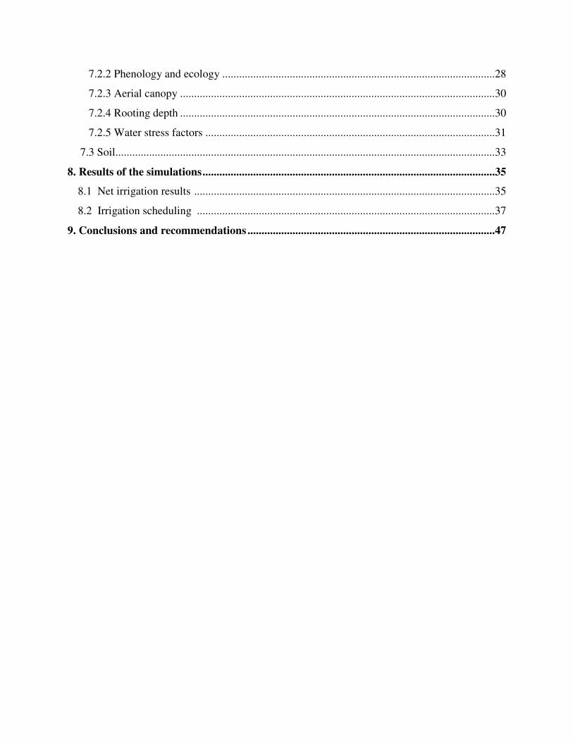
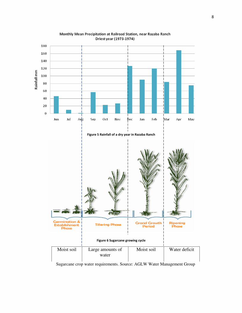
According to the phenology (Figure 5) and environmental conditions required to grow sugarcane
successfully, this crop thrives as the soil water content is readily available on all stages except
ripening, therefore more irrigation water is required because rainfall is unreliable during the dry
season (Figure 6). The hydrograph for a dry year is used to compare irrigation water to be
withdrawn for the different simulations run with Aquacrop for a 15,000 ha of sugarcane farmed
and the instream flows of the Wami River.
The relationship between monthly average rainfall in Razaba Ranch and the phenology of
sugarcane is shown in figures 4 and 5. The biofuel project is going to be other water user of the
Wami River as sugarcane water requirements are imperative for its development.
The National Water Policy (2002) of Tanzania recognizes that irrigation is a highly consumptive
water user and makes greatest impact on net water resources and that agricultural activities also
contribute to pollution from the use of agrochemicals.
8
Figure 5 Rainfall of a dry year in Razaba Ranch
Figure 6 Sugarcane growing cycle
Moist soil Large amounts of
water
Moist soil Water deficit
Sugarcane crop water requirements. Source: AGLW Water Management Group

9
4.1 Ecological functions
The information for the ecological functions (Figure 7) in the lower Wami River is taken from
the USDA Forest Service Technical Assistant Report (Gritzner & Sumerlin, 2007) that was
conducted from January to February 2007.
Wami River Flow and Its Ecological Funtions
Commercial Fisheries
Tourism
Refugia for Wildlife
Figure 7 Lower Wami River ecological functions
4.1.1 Wildlife
Two of three groups of animals rely on the perennial Wami River, tributaries and wetlands for
fresh water drinking and high quality forage during the dry season in Saadani National Park. The
groups are differentiated by their migratory routes; among the animals in these groups are
giraffe, kongoni, lions, wildebeest, zebras, warthogs, buffalos. Also, Saadani is an important area
for a large scale of elephant migration corridors. Some paths of these corridors are located within
the Razaba Ranch where the biofuel project will take place. Wetlands along the river are
important habitat for birds. The Wami River estuary is reported to have at least 20 commonly-
sighted species of birds (Anderson, June 2008). The location of finite, limited dry season habitats
and routes that animals travel to and from are critical for their routes, habitats and behavior in the
short and long term.

10
Table 2. How are the flows in the lower Wami River vital for wildlife in Saadani National and
its surroundings? (Gritzner & Sumerlin, 2007)
Floods Low flows
Maintain riparian zones; including wetlands that
serve as migration corridors, important shelter
habitats and development of vegetation that also
maintain morphological features of the stream.
During dry periods, the low flows provide the
only source of drinking water for game wildlife
and birds.
Diminishing floods have been cited as a cause for
diminished fish runs
Decrease of low flows can strand animals in
residual pools and reduce habitat for wading birds
Cutbanks that are maintained by the riparian
vegetation are important areas where cocrodiles
forage for fish and prawns.
Shelter pools are important for cocrodiles and
hippos, especially during the dry season
Freshwater that flows into the estuary is important
for many fish and shrimp species
If low flows decrease or cease during the dry
periods, the estuary may not be fed by freshwater
thus salinity will increase, so will sedimentation
in the lower reaches of the Wami River
Any type of development near the lower Wami River at any dry season freshwater source may
alter the migration patterns and refugia for the conservation of the wildlife in the park, which in
turn will affect the tourism that sustains the park as well. Altering the floods or low flows needs
to be examined to determine the potential degradation to critical ecological function to Saadani
National Park and its estuary.
4.1.2 Surrounded habitats
Decreasing flows along the Wami River means fewer habitats for wildlife that provide refugia
for their living strategies and behavior, not only within the river channel but also along adjacent
riparian habitats. (Gritzner & Sumerlin, 2007)
11
• Riparian gallery forests along the Wami River are critical habitats for black and white
monkeys, also birds rely on these forests for fruits, roosts, hunting perches and nesting
habitat.
• Dense riparian forests provide important hiding cover for ambush predators.
• Hippos and crocodiles rely on these vegetated areas as corridors to upland feeding
grounds.
4.1.3 Fisheries
Villagers from the regions nearby the Razaba Rancha, fish from the sea and the river.
Information gathered by the USFS team (Gritzner & Sumerlin, 2007)from key informants,
revealed that fish stock of tilapia and catfish is decreasing, which also affect the crocodiles that
also feed from these species. Lack of fish for crocodiles is causing increase in crocodile’s
predation on humans.
On the other hand, villagers from Saadani who rely on fish from the sea have reported decrease
on fish and this may be attributed to reduced floods events in the Wami River. Also, Wami River
fish population seems to be inadequate to support the food chain as raptors and wading bird
species also rely on these fishes. Fish populations in the Wami River are no longer available to
support local populations; therefore villagers are seeking other sources of food.
4.1.4 National Park sustainability
Saadani National Park (SANAPA) is unique because is the only park in Tanzania that contains
both terrestrial and marine ecosystems. The Wami River provides important functions to the park
as already mentioned in previous sections. One of the most important functions to sustain the
park is the ecotourism. This park is the closest to the capital, Dar es Salam, thus tourists have a
closer trip to sight wildlife, not the easier though. People are interested not only in game wildlife
but also for bird watching. Bird’s habitats such as mangroves, banks of the rivers, riparian zones,
can be in threat if the lower Wami River’s flow decline. Also the conversion of dense forests to
agricultural areas will contribute to habitat lost.

12
4.1.5 Livelihoods
Table 3. How are the low flows of the lower Wami River imperative for the livelihoods in
Saadani National Park and other adjacent communities? (Gritzner & Sumerlin, 2007)
Agriculture Shrimp fishery
Lack of fish in the river is changing the traditional
source of food for people in the region, which in
turn is increasing the agricultural activities
Saadani villagers rely mostly in shrimp as source
of food
Conversion of forests into agricultural areas
decreases wildlife habitats
Freshwater fluxes into the estuary are less often
due to lack of floods, thus declining habitat for
shrimp
Larger areas for agriculture mean greater water
needs for food production. In the Wami River
basin, most agriculture withdraws water from the
river, its tributaries and springs.
Floods are diminishing mostly due to large water
withdrawals for agriculture, industry and human
supply purposes upstream; therefore less water
flows into the estuary
5. Biofuel project background
In the first phase of the biofuel project, the government of Tanzania leased to the SEKAB
company a 67 ha plot of land with poor soil and frequent flooding just north of the Ruvu River
near Bagamoyo. The soil is very saline; it dries quickly and becomes crusty. This land is
cultivated with N19 and N25 varieties of sugarcane that will be used as seed for the plantation on
the Wami. A drip irrigation system is in place. The equipment, design and installation all comes
from Israel. All the land has been prepared and sugarcane is being grown on most of it. They are
expecting to obtain yields of 140 tons/ha. Through the drip irrigation, fertilizer (potassium and
urea) is also delivered (fertigation). The drip irrigation system is expensive, but it has been
demonstrated to generate high yields. High temperatures also increase yield. The combination of
equatorial sun and high temperatures with the requisite water and nutrients permits high yields of
quality sugarcane even in poor soil. So far, the company has invested some $300 million USD in
the sugarcane seed farm. (Tobey, 2009)
The sugarcane plantation and ethanol processing plant will be on Razaba Ranch. This is a large
tract of land that the Government of Tanzania gave to Zanzibar in the 60’s. The Razaba Ranch is
13
30,000 ha. Of that, 20,000 hectares were offered to Sekab to use. The remainder (the coastal
strip) is being kept by the government. Sekab’s western boundary is the railroad, the northern
boundary is the Wami, and the eastern boundary is the old coast road (Tobey, 2009)
6. AquaCrop Model
6.1 Conceptual framework
Aquacrop (Raes, Steduto, Hsiao, & Fereres, January 2009) is a computer simulation model that
was used to evaluate the water use requirements of different irrigation practices on sugarcane.
Daily weather data input was obtained from the driest year of a 20 year period—based on daily
flow data and monthly rainfall data. Current practices and various degrees of deficit irrigation
practices that could be applied for drip irrigation were compared. Drip irrigation system is the
technology that SEKAB has proposed to use and which is already in place for 200 ha of an
experimental sugarcane site. Transplanted sugarcane crop was assumed to be irrigated between
June and May followed by harvesting.
Aquacrop evolves from previous the Doorenbos and Kassan (1979) approach by separating (i)
the ET into soil evaporation (E) and crop transpiration (Tr) and (ii) the final yield (Y) into
biomass (B) and harvest index (HI), the mass of the harvested product as a percentage of the total
plant mass of the crop. Harvest Index is the ratio of the yield mass to the total above ground
biomass that will be reached at maturity for non-stressed conditions (Raes, Steduto, Hsiao, &
Fereres, January 2009).
(i) This separation avoids the confounding effect of the non-productive consumptive use of
water (E), especially important during periods of incomplete ground cover.
(ii) This separation avoids the confounding effects of water stress on biomass and harvest index
as their relations with the environment are fundamentally different (Raes, Steduto, Hsiao, &
Fereres, January 2009)
These two concepts deviate from earlier FAO approaches and add to the robustness, simplicity
and accuracy of the model (Raes, Steduto, Hsiao, & Fereres, January 2009). In addition, the time
scale for simulation is based on daily time steps, a period that is closer to the time scale of crop
responses to water deficits (Raes, Steduto, Hsiao, & Fereres, January 2009)

14
Aquacrop is a water-driven model that follows the atmosphere-plant-soil continuum. It also
includes management practices as they affect the crop development, water soil balance and the
final yield. These are the components encompassing the model:
- Climate: rainfall, air temperature, evaporative demand and CO2 concentration
- Crop: development, growth, yield processes and water stress thresholds
- Soil: water characteristics that depend on type of soil
- Management practices: irrigation, fertilization and initial conditions of the soil
Pests, diseases and weeds are not considered.
6.2 Opportunities and Challenges
This software developed by FAO, first released in January 2009, has been used to model
different crops worldwide for different purposes. The software is free and there is support
assistance for users. The model is user friendly and intuitive, data requirements are reasonable,
information is available on the web, and is compatible with other tools provided by FAO such as
ETo calculator and ClimWAT, which are explained later.
For these reasons aside from the conceptual framework, Aquacrop is suitable for determining
sugarcane water requirements under different scenarios in a study area like Razaba Ranch in
Tanzania. Limited resources to carry out this project were the main challenge as data for each
component were not readily available.
6.3 Assumptions
It was necessary to make several assumptions due to the data variability in terms of time frame
and location.
- The climate data are from two different locations and time frame. The rainfall data are from a
gauging station near Razaba Ranch and it was obtained in a monthly basis, whereas the
evaporative demand and air temperature come from the same source which is ClimWAT, the
former calculated and imported using ETo calculator which is a software developed by the
Land and Water Division of FAO. Its main function is to calculate Reference

15
evapotranspiration (ETo) according to FAO standards (FAO-UN, FAO Water, Software,
2010). These options are useful to overcome the problem of no data from the area of study. It
was assumed that both sites the gauging station for the rainfall data and ClimWAT have
similar environmental and climatic conditions.
- Soil characteristics in Razaba Ranch were assumed to be loamy sand based on the description
of the FAO classification for Arenosol which is the soil type that dominates the sugarcane
farm. (FAO-UN, Digital Soil Map of the World, 2010)
- The major assumption made for the crop component is that sugarcane is had to be classified
for modeling as a “tuber and root crop” because it is a type of vegetative crop which is not
yet available in the model. Among the crop types to choose from, the difference between
grain producing crops, leafy vegetable and root and tubers is linked to the flowering and
building up of the harvest index. Neither grain product crop nor leafy vegetable type apply
for sugarcane, as the former simulates flowering and the latter does not allow to set up an
initial accumulation of the yield. A sugarcane crop should not flower but should have an
accumulation of sugar in the stem which represents the final yield.
- The soil water content across the farm area is assumed to be at either field capacity or 50% of
total available water to the plants as transplanting is preceded by the long rainy season.
- Irrigation scheduling is created for different scenarios.
6.4 Scenarios
6.4.1 Net Irrigation
The total amount of irrigation water required to keep the water content in the soil profile above a
certain threshold (50% of Readily Available Water) is the net irrigation water required for the
cropping period. This net requirement does not consider extra water that has to be applied to the
field to account for conveyance losses or the uneven distribution of irrigation on the field. When
the root zone depletion exceeds a given threshold value (Figure 8), a small amount of irrigation
water will be stored in the soil profile to keep the root zone depletion just above the specific
threshold (Raes, Steduto, Hsiao, & Fereres, January 2009).

16
a) b)
Figure 8 Net irrigation determinants for sugarcane crop (a) 0% RAW (b) 50% RAW
6.4.2 Irrigation schedule
The goal of an efficient irrigation scheduling planning is to “provide knowledge on correct time
and optimum quantity of water application to optimize crop yield with maximum water use
efficiency and at the same time ensure minimum damage to the soil” (Netafim)
Management, irrigation and fertilization are practices that affect the development of the crop and
therefore the final yield. Because of limiting factors such
as water availability through rainfall and sandy soil
conditions, these management practices should be designed
according to the needs. SEKAB is proposing to irrigate the
crop using the Wami River as the main source and through
a sophisticated drip irrigation (Figure 9) system which is
going to be able to also apply fertilizer directly to the root
zone.
In order to estimate the crop water requirements for 15,000 hectares of sugarcane farm, different
scenarios were simulated using Aquacrop model. The scenarios generated are based on changes
to three factors that can influence the outcome of the modeling. These include factors that
emerge from management decisions (Factors 1 and 3) as well as a factor (Factor 2) that depends
on climatic conditions:
Drip irrigation for sugarcane
seed experiment site, SEKAB
Figure 9 Drip irrigation for sugarcane
seed experiment site, SEKAB
Threshold stomata
closure 100% RAW
Threshold leaf
expansion growth
Field capacity
0%RAW
Allowable root zone depletion
Saturation
FC
RAW
TAW
PWP

17
1. Irrigation frequency: Daily and 7 day-interval
2. Initial conditions of the soil: At field capacity (FC) or 50% of total available water
(TAW)
3. Applying irrigation dose equivalent to a percentage of the soil moisture depletion of the
root zone, e.g. an irrigation of 100% depletion to bring the soil moisture reservoir to field
capacity. Irrigation doses selected were 100% and 50%.
Combinations of the three factors were simulated and the results were analyzed. Each factor was
defined given similar studies using different models; however this study is not intended to
compare their results. Because the exact period of each phenological stage for this specific project
is not specifically known, irrigation water was homogenously applied throughout the growing
season.
Factor 1: Frequency of irrigation events.
Frequency of irrigation events, daily or 7 day-intervals were used for simulation. Because
sugarcane has different water requirements over the growing cycle, for the stem, canopy, root
and yield formation, it is necessary to investigate whether there is a change in yield if frequency
also changes.
Factor 2: Initial soil water conditions.
The initial soil water conditions depend on the climate and management practices. Since the
growing season begins in June, after the main rainy season occurs in the Razaba Ranch area, it is
most likely that the soil is at field capacity. On the other hand, if the soil has been exposed to
extended evapotranspiration, the soil water content may drop to 50% of TAW which is also
assumed. Despite the large amount of precipitation, the soil is unlikely to be saturated due its
sandy characteristics. Along the floodplains of the Wami River, where the soil is richer and
flooding frequently occurs, initial conditions of the soil can be at saturation, however this
assumption was not considered in the model.

18
Factor 3. Soil moisture content following irrigation.
This is the difference between the amount of water applied and the amount of irrigation water
required to bring the root zone back to field capacity. In the model, a value of zero indicates that
the applied irrigation will bring the soil water content in the root zone at field capacity (reached
at the end of the day), whereas a negative value indicates that an under irrigation is planned. This
strategy applied zero and -5mm throughout the growing season. The value of -5mm refers to the
amount of water through the root zone and is adopted only to investigate how the crop performs
under less water availability.
These are the combinations of the factors that create the scenarios analyzed for this study:
Scenario Initial
conditions
Depth Criteria Irrigation regime
(Time Criteria)
1 Field Capacity Back to Field
Capacity
Daily
7 days
2 Field Capacity 5mm of water deficit
below FC
Daily
7 days
3 TAW 50% Back to Field
Capacity
Daily
7days
4 TAW 50% 5mm of water deficit
below FC
Daily
7 days
In addition to these scenarios, two more were created to match frequency and depth of irrigation
to sugarcane specific stages of water requirements as stated in the text box below. These
scenarios are intended to investigate if irrigation practices taking into account the crop
phenology and available water in the river would result in similar final yield as an homogeneous
irrigation application.
Frequency and depth of irrigation should vary with growth periods of the cane.
- Establishment period: light frequent irrigation applications are preferred
19
- Early vegetative period: tillering is in direct proportion to the frequency of irrigation
- Stem elongation and early yield formation period: irrigation interval can be extended but
depth of water should be increased
- Ripening period: irrigation intervals are extended or irrigation is stopped when it is necessary
to bring the crop to maturity by reducing the rate of vegetative growth, dehydrating the cane
and forcing the conversion of total sugars to recoverable sucrose
Source: (FAO-UN, Land and Water Development Division, 2002)
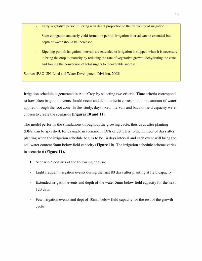
Irrigation schedule is generated in AquaCrop by selecting two criteria. Time criteria correspond
to how often irrigation events should occur and depth criteria correspond to the amount of water
applied through the root zone. In this study, days fixed intervals and back to field capacity were
chosen to create the scenarios (Figures 10 and 11).
The model performs the simulations throughout the growing cycle, thus days after planting
(DNr) can be specified, for example in scenario 5, DNr of 80 refers to the number of days after
planting when the irrigation schedule begins to be 14 days interval and each event will bring the
soil water content 5mm below field capacity (Figure 10). The irrigation schedule scheme varies
in scenario 6 (Figure 11).
• Scenario 5 consists of the following criteria:
- Light frequent irrigation events during the first 80 days after planting at field capacity
- Extended irrigation events and depth of the water 5mm below field capacity for the next
120 days
- Few irrigation events and dept of 10mm below field capacity for the rest of the growth
cycle

20
These criteria are adjusted to the phenological stages and their water requirements.
Figure 10 Irrigation schedule for scenario 5 in AquaCrop (FAO-UN, AquaCrop Software, 2009)
• Scenario 6 consists in the following criteria:
- Light frequent irrigation events during the first 80 days after planting keeping the soil at
5mm of water below field capacity
- Light frequent irrigation events and depth of the water 15mm below field capacity for the
next 120 days
- Few irrigation events and dept of 20mm below field capacity for the rest of the growth
cycle
These criteria are defined to match with water availability in the Wami River during the dry and
wet months and teasing the depth of water in the root zone.

21
Figure 11 Irrigation schedule for scenario 6 in AquaCrop (FAO-UN, AquaCrop Software, 2009)
7. Data and Methodology
This scheme represents the methodology of this study. First, the sugarcane characteristics are
incorporated within the model to simulate its performance for the physical and climatic
conditions established by the input data. Aquacrop is the program used to put all the components
together and the different scenarios which are later compared with the flows of the Wami River.
The amount of water withdrawal required to irrigate 15,000 ha of sugarcane are then compared
with flows available during a dry year.

22
Climate
Crop
Soil
Irrigation
Field
Sugarcane Characteristics
Wami River Flows
Water Withdrawal
Scenarios
Low Flows
Morphology
Phenology
Figure 12 Components for estimating water requirements for sugarcane growth
7.1 Climate
The atmospheric environment of the crop’s
site is described in the climate component and
deals with key input meteorological variables.
Five weather input variables are required to
run Aquacrop, and are separately described
below. These data are linked temporally
which means the growing season depends on
the climatic conditions given by these data.
Since SEKAB’s proposal (SEKAB,
November 2008) is to grow sugarcane starting
from June and a year is the maximum period
that takes for harvesting but not less than six
months, two years of data are required (1973-
1974). Figure 13. Shows the location of rainfall, air temperature and ETo (CLIMWAT FAO) in
Tanzania
ClimWAT FAO Station
Rainfall Station
Bioethanol Plant

23
7.1.1 Rainfall
Aquacrop is robust enough to allow the creation of scenarios from data of different time scales.
The amount of precipitation during the growing cycle of sugarcane represents one of the most
important inputs of water to the soil. The rainfall data is collected in rain gauging stations, in this
case a nearby station to the Razaba Ranch. Monthly rainfall is available from 1964 to 1981.
Data are missing for 1968 and 1969 and in some years the months of April and May have suspect
data.
Because Aquacrop accounts for daily time steps instead of long periods (of the order of months),
the monthly data are interpolated to obtain daily rainfall data, which is a period that is closer to
the time scale of crop responses to water stress. The interpolation procedure is performed by the
model itself. On the other hand it is important to keep in mind that the model arranges the period
of the simulation to be the same as the rainfall data. For instance, during the period of 1973-1974
which is the year of rainfall data, the growing cycle starts in June and finishes towards the end of
May, and thus the simulation uses the data during this period to generate the outputs.
Precipitation in the lower Wami River averages 800-1000mm per annum and is bimodal with
two rainy seasons (Figure 14):
Figure 13 Rainfall input for Aquacrop, from the Wami lower basin Tanzania (FAO-UN, AquaCrop Software, 2009)
1 Jan 31 Dec Month

24
The long rains occur during March to May/June which account for about 60% of the total rainfall
in the year. On the other hand, the short rains happen during the period September/October –
December and these rains are unreliable and poorly distributed.
7.1.2 Air temperature
The model requires both maximum and minimum air temperature as these parameters determine
crop growth and phenology. Because data were not available for the same gauging station of the
rainfall data, nor were available through officials in Tanzania, temperature data were obtained
from a location with similar climatic, geographical and environmental conditions with available
data.
ClimWAT (FAO-UN, FAO Water, Databases, 2010) is a database that contains worldwide
climatic data that provides long-term monthly mean values of seven climatic parameters:
- Mean daily maximum temperature in Celsius
- Mean daily minimum temperature in Celsius
- Mean relative humidity %
- Mean wind speed in km/day
- Mean sunshine hours per day
- Mean solar radiation in MJ/m2/day
- Monthly rainfall in mm/month
- Monthly effective rainfall mm/month
- Reference evapotranspiration calculated with Penman-Monteith method mm/day
From the database, multiple stations are found in Tanzania; however Tanga is the closest station
to Razaba area at about 60 miles north. Moreover, Tanga region has similar environmental
conditions to the area of study, it is a coastal town with low development, and thus climatic
conditions may resemble the ones in the Razaba area especially in terms of air temperature..
Based on this assumption, the minimum and maximum air temperature data are shown in Figure
15 in which temperature ranges from 19.8° to 32.9°. Temperatures in the coastal area of

25
Tanzania are most of the time homogeneous throughout the years; therefore using a long-term
monthly mean data should not introduce major errors into the results.
Figure 14 Air temperature input for Aquacrop, from Tanga Tanzania (FAO-UN, AquaCrop Software, 2009)
7.1.3 Reference evapotranspiration (ETo)
The evapotranspiration rate from a reference surface (living grass), not short of water, is called
reference evapotranspiration (ETo). ETo is used in Aquacrop as a measure of the evaporative
demand of the atmosphere by means of the FAO Penman-Monteith equation.
Actual site-specific weather data from a local station are not available to calculate ETo, thus the
data provided by ClimWAT is used such as maximum and minimum air temperature, solar
radiation, wind run and maximum and minimum air humidity.
Aquacrop does not have the capability to calculate ETo values, however FAO provides the ETo
Calculator for this purpose. This tool is compatible with data from ClimWAT as it contains
weather data for the chosen station that can be used to estimate ETo. The outputs from the ETo
Calculator can be exported into Aquacrop within the climate component. These three tools:
Aquacrop, ClimWAT and ETo calculator are free and downloadable from the FAO website,
which is very convenient for users that cannot afford expensive software and data.
In the graph is shown below (Figure 16) the reference evapotranspiration ranges from 3.8
mm/day to 5.6 mm/day which represent the evaporating power of the atmosphere at Tanga and
these are also long-term monthly mean records. Because ETo, is a reference rate of ET it does not
1 Jan 31 Dec Month
T max
T min

26
consider crop characteristics and soil factors (Allen, Pereira, Raes, & Smith, 1998). Actual ET
emerges by linking ETo to plant and water stress conditions.
Figure 15 ETo input data for AquaCrop, from Tanga Tanzania (FAO-UN, AquaCrop Software, 2009)
7.1.4 Mean Annual Atmospheric CO2 Concentration
This weather parameter influences the crop growth rate and crop water productivity. CO2
concentration is measured at Mauna Loa Observatory in Hawaii and used as default in Aquacrop
because the air at the site is very pure to its remote location in the Pacific Ocean, high altitude
(3397 m.a.s.l) and great distance from major pollution sources (Raes, Steduto, Hsiao, & Fereres,
January 2009).
Figure 16. Atmospheric CO2 concentration, default data from AquaCrop (FAO-UN, AquaCrop Software, 2009)
1 Jan 31 Dec Month
mm/day
4 mm
2 mm
6mm
8 mm
Reference:
369.41ppm
From 1990 To 2010 Range displayed
320 ppm
340 ppm
360 ppm
Reference
380 ppm
27
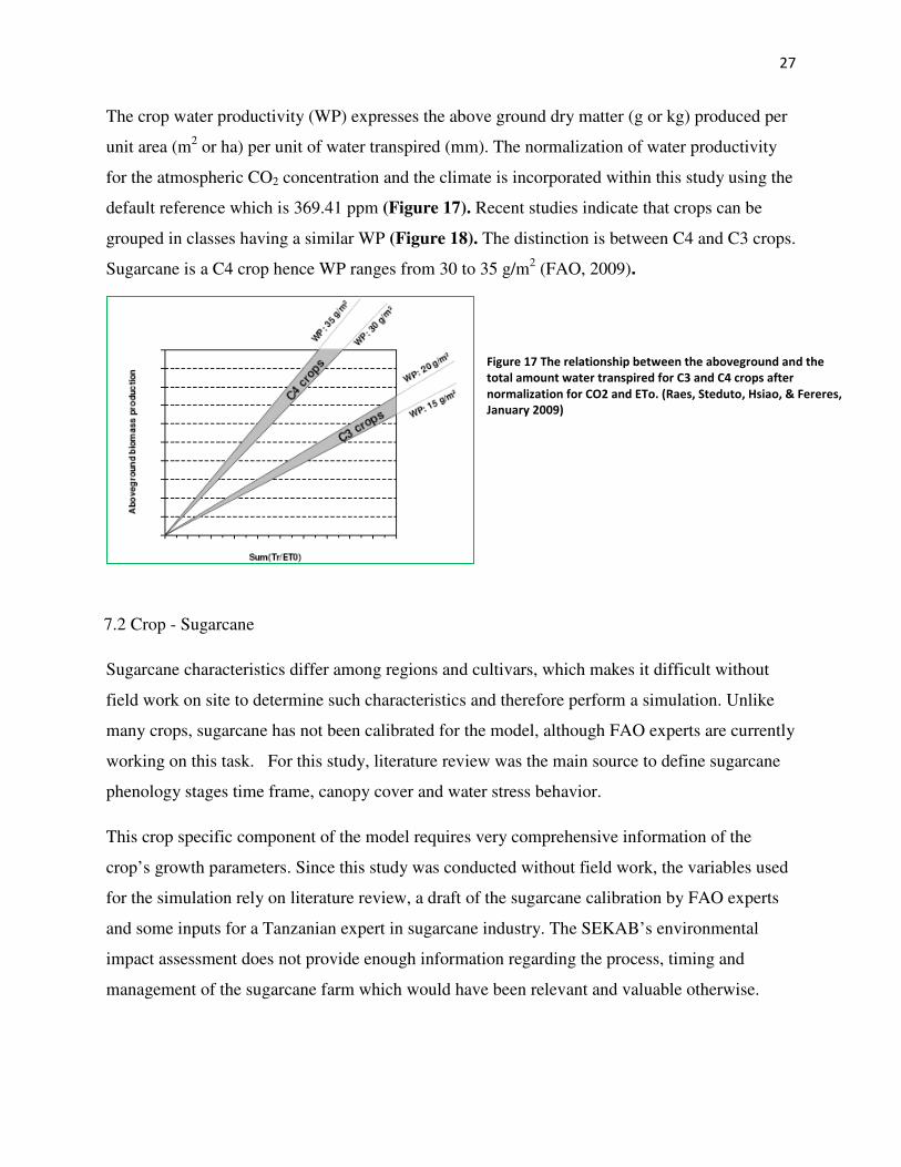
The crop water productivity (WP) expresses the above ground dry matter (g or kg) produced per
unit area (m2 or ha) per unit of water transpired (mm). The normalization of water productivity
for the atmospheric CO2 concentration and the climate is incorporated within this study using the
default reference which is 369.41 ppm (Figure 17). Recent studies indicate that crops can be
grouped in classes having a similar WP (Figure 18). The distinction is between C4 and C3 crops.
Sugarcane is a C4 crop hence WP ranges from 30 to 35 g/m2 (FAO, 2009).
7.2 Crop - Sugarcane
Sugarcane characteristics differ among regions and cultivars, which makes it difficult without
field work on site to determine such characteristics and therefore perform a simulation. Unlike
many crops, sugarcane has not been calibrated for the model, although FAO experts are currently
working on this task. For this study, literature review was the main source to define sugarcane
phenology stages time frame, canopy cover and water stress behavior.
This crop specific component of the model requires very comprehensive information of the
crop’s growth parameters. Since this study was conducted without field work, the variables used
for the simulation rely on literature review, a draft of the sugarcane calibration by FAO experts
and some inputs for a Tanzanian expert in sugarcane industry. The SEKAB’s environmental
impact assessment does not provide enough information regarding the process, timing and
management of the sugarcane farm which would have been relevant and valuable otherwise.
Figure 17 The relationship between the aboveground and the
total amount water transpired for C3 and C4 crops after
normalization for CO2 and ETo. (Raes, Steduto, Hsiao, & Fereres,
January 2009)
28
In this case the cultivar-specific parameters of sugarcane are assumed to be under favorable
conditions to grow in a tropical country like Tanzania.
The model, Aquacrop, simulates the crop’s development and responses to environmental factors
through five major components: phenology, aerial canopy, rooting depth, biomass and
harvestable yield. As the crop responds to water stress, which can occur at any time during the
crop cycle, three major feedbacks are driven by this: reduction of the canopy expansion rate,
acceleration of senescence and closure of the stomata (Raes, Steduto, Hsiao, & Fereres, January
2009).
7.2.1 Overview
Sugarcane(Saccharum officinarum) is a C4 plant that grows from tropical to subtropical regions
of the globe between 33°N and S of the equator (Griffee, 2000). The climatic and weather
regimes in Tanzania are suitable for sugarcane growth, however water from rainfall is a limiting
factor in this area since the crop requires large amounts of water to achieve high yield.
Worldwide sugarcane occupies 20.42 million hectares with a total yield of 1333 million metric
tons (Netafim). This crop is an important commercial product in Tanzania, since this is the main
source of sugar production mainly for home consumption and small proportion is exported.
Tanzania’s annual sugar production ranges from 250,000 to 300,000 tons and these estimates are
expected to increase given more irrigation supply and management (Tarimo & Takaruma, 1998).
Sugarcane is a natural, renewable agricultural source that not only provides sugar production but
also numerous by products such as ethanol, fertilizer, and more.
7.2.2 Phenology and ecology
The principal climatic components that control cane growth, yield and quality are temperature,
light and moisture availability (Netafim). Each growth phase of sugarcane requires different
climatic conditions to develop properly and thus the location of the farm and the timing of
growth are important considerations for producing sugarcane.

29
Figure 19 shows the phenology of sugarcane under normal conditions and the climatic factors
for each phase:
These ecological requirements of sugarcane make Tanzania best suited for its production
(Netafim):
• Relative humidity: high humidity is favorable for rapid cane elongation during yield
development. As for the ripening phase, a moderate humidity is recommended.
• Temperature: this is a very important factor for sugarcane growth. For germination of the
stem, ideal temperature is 27-34ºC; however the process slows above 35ºC and stops at 38ºC.
High temperatures reduce photosynthesis and increase respiration. This would be a minimal
concern for Razaba Ranch since temperatures are normally not higher than 33º C. Optimum
growth is achieved with mean daily temperatures in the range of 22-30ºC with a minimum of
20ºC (Pursglove and Evans, 1974) Citation 24. During the ripening phase however,
temperatures should be cooler to increase sucrose content in the cane.
TimeframeLasts 30-35
daysLasts up 120 days
Lasts up to
270 days
Starts from ~
270-360 days
Lasts up to 3
months
Humidity 80-85% 45-65%
Temperature32 – 38 C 22 – 30 C; Minimum 20 C
20 – 10 C
Enrichment of
sucrose
Rainfall or Irrigation 1200-1500mm Limited or non
Sunlight Paramount importance RequiredAmple sunshine
and cool nights
Soil type >1m depth with deep rooting, total available water 15%, pH 5-8.5
Factors that contribute to
growth by phasesSaccharum officinarum
Figure 18 Sugarcane phenology and factors that determine its development

30
• Rainfall: abundant water is required in the months of vegetative growth and less water
during the ripening phase. Precipitation between 1200-1500 mm annual is (Tarimo &
Takaruma, 1998). The duration of the rainy season could be as high as 1300 mm per year and
as low as 570mm per year in the Razaba Ranch area, indicating that supplementary irrigation
is necessary during the growing season, especially in the dry months. One season can be
between 12 to 13 months from transplanting to harvesting; therefore the crop is exposed to
dry periods in which physiological stages require large amount of water for effective
development, water stress occurring during stem elongation dramatically reduces cane
production.
• Sunlight: because sugarcane is a sun loving plant, this parameter plays an important role in
the overall growth. Being a C4 plant, sugarcane is capable of photosynthetic rates and the
process shows a high saturation range with regards to light. The greater the exposure of the
sugarcane to sunlight, the greater the yield.
7.2.3 Aerial Canopy
Table 4. FAO sugarcane canopy cover (FAO-UN, Land and Water Development Division, 2002)
Crop age Growth stage in terms of canopy cover
months
0 - 1 harvest to 0.25 full canopy
1 - 2 0.25 - 0.5 full canopy
2 - 2.5 0.5 - 0.75 full canopy
2.5 - 4 0.75 to full canopy
4 - 10 full canopy
10 - 11 early senescence
11 - 12 ripening
7.2.4 Rooting depth
The rooting system is simulated in AquaCrop through its effective root zone and water extraction
pattern. The effective root zone (Z) is defined as the soil depth where most of the root water
uptake takes place. Active root zone for water uptake is generally limited to the uppermost
layers, about 2m in which 100 percent of the water is normally extracted (Raes, Steduto, Hsiao,

31
& Fereres, January 2009). Rooting depth varies with soil type and irrigation regime; infrequent,
heavy irrigations normally results in a more extensive root system.
The relationship between the percentage of canopy cover and the rooting depth over the growing
cycle of sugarcane as simulated in Aquacrop is shown in Figure 20. Maximum rooting depth is
reached 180 days after planting.
Figure 19 Relationship between effective rooting depth and canopy cover for sugarcane (FAO-UN, AquaCrop Software, 2009)
7.2.5 Water stress factors
Effects of water stress on canopy expansion, stomatal conductance, and early canopy senescence
are described by water stress coefficients Ks. These coefficients depend on thresholds chosen for
the specific crop.
Thresholds: are expressed as a fraction of the Total Available soil Water (TAW). TAW is the
amount of water soil can hold between field capacity (FC) and permanent wilting point
(PWP). For each physiological pattern of sugarcane different Ks were assumed.
Canopy Expansion: Leaf growth by area expansion and therefore canopy development are the
highest sensitivity to water stress among all the plant processes described by the model.
• Sugarcane is very sensitive to water stress during canopy expansion. Water deficit
during the establishment period and early vegetative period (tillering) have an
adverse effect on yield.

32
Stomata closure: stomata has been shown to be much less sensitive to water stress in
comparison to leaf expansive growth.
• Sugarcane is moderately sensitive to water stress. Water deficit during the
vegetative period (stem elongation) and early yield formation causes a lower rate of
stalk elongation
Early canopy senescence: under moderate severe water stress conditions, leaf and canopy
senescence is triggered, thereby reducing the transpiring foliage area.
• Sugarcane is moderately tolerant to water stress. During the ripening period, low
moisture content is necessary. However, when the plant is too seriously deprived of
water, loss in sugar content can be greater than sugar formation.
In Figure 21, water stress effects simulated by AquaCrop are shown. Ks is an adimensional
variable in which 1 indicates no stress and 0 indicates full stress. The more sensitive the
physiological factor is to water stress the closer to field capacity it requires to be at to avoid such
stress.
Simulating water stress effects
Ks
Leaf expansionStomata closure
Senescence
Figure 20 Water stress factor for sugarcane under normal conditions (FAO-UN, AquaCrop Software, 2009)

33
8. Soil
Narrative information indicates that sandy soil composes most of northern portion of the
proposed plantation. This can be farmed with sugarcane, but it is more costly because it requires
good irrigation and fertilizer. Closer to the Wami the soil is dark and rich. The vegetation is
thick. This area is flooded annually. The dark soil is deep, over 5-6 feet. (Tobey, 2009).
Figure 21 Soils Map for Razaba Ranch (FAO-UN, Digital Soil Map of the World, 2010)
The Soil and Terrain (SOTER) digital database of Tanzania was the source to identify soil types
within Razaba Ranch and its scale is 1:2,000.000 (Figure 21). According to this map Arenosol
34
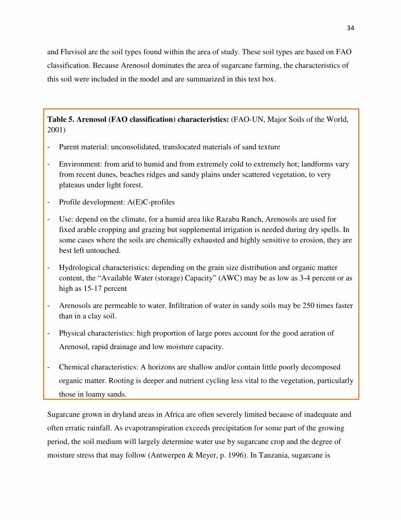
and Fluvisol are the soil types found within the area of study. These soil types are based on FAO
classification. Because Arenosol dominates the area of sugarcane farming, the characteristics of
this soil were included in the model and are summarized in this text box.
Table 5. Arenosol (FAO classification) characteristics: (FAO-UN, Major Soils of the World,
2001)
- Parent material: unconsolidated, translocated materials of sand texture
- Environment: from arid to humid and from extremely cold to extremely hot; landforms vary
from recent dunes, beaches ridges and sandy plains under scattered vegetation, to very
plateaus under light forest.
- Profile development: A(E)C-profiles
- Use: depend on the climate, for a humid area like Razaba Ranch, Arenosols are used for
fixed arable cropping and grazing but supplemental irrigation is needed during dry spells. In
some cases where the soils are chemically exhausted and highly sensitive to erosion, they are
best left untouched.
- Hydrological characteristics: depending on the grain size distribution and organic matter
content, the “Available Water (storage) Capacity” (AWC) may be as low as 3-4 percent or as
high as 15-17 percent
- Arenosols are permeable to water. Infiltration of water in sandy soils may be 250 times faster
than in a clay soil.
- Physical characteristics: high proportion of large pores account for the good aeration of
Arenosol, rapid drainage and low moisture capacity.
- Chemical characteristics: A horizons are shallow and/or contain little poorly decomposed
organic matter. Rooting is deeper and nutrient cycling less vital to the vegetation, particularly
those in loamy sands.
Sugarcane grown in dryland areas in Africa are often severely limited because of inadequate and
often erratic rainfall. As evapotranspiration exceeds precipitation for some part of the growing
period, the soil medium will largely determine water use by sugarcane crop and the degree of
moisture stress that may follow (Antwerpen & Meyer, p. 1996). In Tanzania, sugarcane is

35
typically grown on loamy soils with good proportions of sand and clay (Tarimo & Takaruma,
1998), however Razaba Ranch as it was described above has sandy soils which indicate other
limiting factor for crop’s development under appropriate conditions.
8. Results of simulations
Sugarcane crop water requirements depend on climatic conditions, soil characteristics,
management practices and most importantly how the plant’s physiology responds to these
factors. The sugarcane crop outputs of simulations taking into account these considerations and
run with AquaCrop software are shown and analyzed in this section.
Seasonal water withdrawal from the lower Wami River is estimated by calculating the irrigation
water demand for a 15,000 ha sugarcane farm. This water extraction is compared with historical
flow data from the gauging station at Mandera for a dry year scenario.
A 12 month harvest season was assumed for these simulations with a growing season
commencing in June after the primary rainy season. A 12 month growing season is applied
because that is what the literature refers to in characterizing the crop’s growth.
8.1 Net irrigation results
The amount of water needed to bring the soil to field capacity is defined as “net irrigation,”
which depends on environmental conditions at the farm. Field capacity is the maximum amount
of water that can be retained against gravitational forces. It is not necessarily the amount of water
in the soil that sugarcanes needs to grow properly without water stress at all times of the growing
cycle. Readily available water (RAW) is the water represents soil water in the root zone and is
the water required for the plant to grow without crop stress. Different scenarios of RAW were
applied to assess the impact on net irrigation requirements and crop yield.
Table 6 shows the results of sugarcane net irrigation at Razaba Ranch BioEnergy project using
the AquaCrop model and different assumptions of Readily Available Water.

36
Table 6 AquaCrop estimates of net irrigation requirements for sugarcane growth at Razaba Ranch
based on scenarios of daily regimes of readily available water (RAW)
Allowable root zone
depletion Initial conditions
Net Irrigation
(mm)
Yield
(ton/ha)
FC*
(0%) RAW**
FC 760 23
TAW***
50% 760 22.5
10% RAW FC 640 23
TAW 50% 680 22.5
35% RAW FC 610 23
TAW 50% 655 22.5
50% RAW FC 595 23
TAW 50% 640 22.5 *Field Capacity;
** Readily Available Water;
***Total Available Water
The results show that net irrigation needs to be higher when water content in the root zone is
managed at close to field capacity. However, if the initial conditions of the water content based
on the soil profile, are below field capacity (50% of total available water), slightly more water is
required to achieve the depth that triggers water stress.
The comparison between two scenarios in which allowable root zone depletion is at 50% RAW
(Figure 23) and at field capacity (Figure 24) demonstrates that the model predicts that sugarcane
does not need to maintain soil water content at field capacity for successful development.
Although it is not shown in the Table 5, the modeling approach assumes that the crop will
experience severe water stress when RAW is below 50%.
The Aquacrop model results are not sensitive to yield if net irrigation conditions are adequately
altered. However, this result will also depend on site crop development criteria such as timing of
specific stages, canopy cover and yield built up.
Calculating net irrigation requirements at different levels of RAW was useful to determine the
crop’s thresholds in regard to water content in the soil. It is important to note, however, that the
irrigation technology used at the farm will also affect net irrigation since different irrigation
systems apply water will differing degrees of efficiency.
The management implication is that understanding sugarcane’s water stress thresholds
throughout the growing season helps plantation managers and water resource authorities to
estimate overall crop water requirements.
37
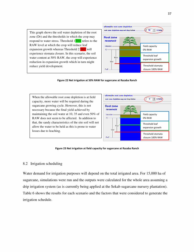
Figure 22 Net Irrigation at 50% RAW for sugarcane at Razaba Ranch
Figure 23 Net irrigation at field capacity for sugarcane at Razaba Ranch
8.2 Irrigation scheduling
Water demand for irrigation purposes will depend on the total irrigated area. For 15,000 ha of
sugarcane, simulations were run and the outputs were calculated for the whole area assuming a
drip irrigation system (as is currently being applied at the Sekab sugarcane nursery plantation).
Table 6 shows the results for each scenario and the factors that were considered to generate the
irrigation schedule.
This graph shows the soil water depletion of the root
zone (Dr) and the thresholds in which the crop may
respond to water stress. Threshold 1TH1 refers to the
RAW level at which the crop will reduce leaf
expansion growth whereas Threshold 2 TH2 will
experience stomata closure. In this scenario, the soil
water content at 50% RAW, the crop will experience
reduction in expansion growth which in turn might
reduce yield development.
When the allowable root zone depletion is at field
capacity, more water will be required during the
sugarcane growing cycle. However, this is not
necessary because the final yield achieved by
maintaining the soil water at 10, 35 and even 50% of
RAW does not seem to be affected. In addition to
that, the sandy characteristics of the site soil will not
allow the water to be held as this is prone to water
losses due to leaching.
Threshold leaf
expansion growth
Threshold stomata
closure 100% RAW
Field capacity
0% RAW
Threshold leaf
expansion growth
Threshold stomata
closure 100% RAW
Field capacity
0% RAW

38
Table 7 AquaCrop results for sugarcane irrigation supply and final yield at Razaba Ranch
In Figure 25, scenarios 1 and 2 for daily irrigation requirements are shown and compared with
available water in the Wami River during a dry year. Special attention is paid to low flow events
when irrigation demand exceeds Wami river flows. The following results are found:
- At the beginning of the growing season, when sugarcane is transplanted from the seed farm,
the main rains of April and May still have influence on river flow, and the soil water content
will likely be at field capacity in the planting area. Scenario 1, which simulates maintaining
the soil at field capacity in every irrigation event, will require more water withdrawal than
scenario 2 which keeps the soil water content 5mm of water below field capacity.
- At the end of September during the dry season and low flows, irrigation demand begins to
exceed available water in the river at a level of almost double the flow availability for both
scenarios. Water extraction for irrigation of 15,000 ha of sugarcane would completely dry the
river with zero flow to the estuary. The lowest flow recorded was 1.6m3/sec during this
period and the irrigation demand is 7.4m3/sec for both scenarios.
Scenario Initial
conditions Depth Criteria (Back
to Field Capacity) Irrigation regime (Time Criteria)
Irrigation Supply
Yield
mm ton/ha
1 Field Capacity Back to field capacity Daily 1365 23
Weekly 670 23
2 Field Capacity 5mm less than field
capacity
Daily 670 23
Weekly 490 23
3 TAW 50% Back to field capacity Daily 1290 23
Weekly 620 23
4 TAW 50% 5mm less than field
capacity
Daily 735 23
Weekly 570 23
5 Field Capacity 7 days (FC)
14 days (-5mm) 21 days (-10mm)
Matched to phenology
450 23
6 Field Capacity 3 days (-5mm) 2days (-15mm)
14 days (-20mm) Matched to flows 460 23

39
m3/sec Scenario 2: Daily irrigation events
Figure 24 Comparison of daily irrigation demand and lower Wami River flows for a dry year - scenarios 1 and 2
(15,000 ha of sugarcane)
Irrigation water demand
Wami River flows (Dry year)
Scenario 1: Daily irrigation events

40
- During the second short rainy season that brings more water discharge in the river, the water
demand in scenario 1 is ten times higher than scenario 2. Under the latter scenario, soil water
content is maintained by rainfall sufficient to maintain proper development without stress. As
a consequence, insignificant Wami River water withdrawal for irrigation is required.
Scenario 1 demands more irrigation water but the sugarcane crop does not develop better
when the soil water content is maintained at field capacity.
- In March, unreliable flows and a high demand for irrigation water are in conflict for both
scenarios. Low discharge values in the Wami River less than 1m3/sec were recorded in
March and irrigation demand for scenarios 1 and 2 are 9.5 m3/sec and 5.5m
3/sec respectively.
- By the end of the growing season, scenario 1 still demands water despite the amount of
rainfall, which is the highest in the year. On the other hand, scenario 2 does not require water
to be withdrawn. In the former, the highest flow recorded was 495m3/sec and irrigation
demand is 7.5m3/sec.
Management implications:
- Daily irrigation events may be desirable for sugarcane growth when water use efficiency is
considered using the soil profile as water reservoir.
- Irrigation planning for sugarcane in Razaba Ranch should take into account that this crop
does not require the soil water content to be at field capacity, thus more water use efficiency
and less water to be withdrawn for needless irrigation supply.
- Wami River will go dry during the low flows if management practices similar to scenarios 1
and 2 for daily irrigation events are carried out.
The daily irrigation demand in scenario 3 and 4 differs slightly from scenarios 1 and 2. Table 6
shows total irrigation supply and crop yield for these scenarios. Because the initial soil water
content factor depends on the environmental conditions, scenarios 3 and 4 were simulated at
50% of the total available water, hence the higher the irrigation demand.

41
In Figure 26, scenarios 1 and 2 are shown and the irrigation water demand for a 7 day interval is
compared with the available water in the Wami River during a dry year scenario. The flows were
m3/sec
m3/sec
Scenario 1: 7 day interval
Scenario 2: 7 day interval
Irrigation water demand
Wami River flows (Dry year)
Figure 25 Comparison of irrigation demand for a weekly interval and lower Wami River flows for a dry year – scenarios 1
and 2 (15,000 ha of sugarcane)

42
averaged for a 7 day period to determine the likelihood of water available in the river. The
following results are found:
- Irrigation schedule for a 7 day interval regime exceeds water requirements of a daily regime
for these specific irrigation events. This will incur more extractable water from the Wami
River every 7 days in greater quantities compared with the daily events.
- Comparing both figures 25 and 26, the pattern of irrigation water demand is similar, however
as already mentioned, the crop requires more water during the irrigation events as it was
exposed to 6 days of zero irrigation. The average flow during the 7 day interval indicates the
amount of water that will likely be available during the irrigation events.
- During low flows from September through November, the average of the lowest flow is
2m3/sec and irrigation water demand to be withdrawn from the Wami River is 45m
3/sec in
both scenarios. This indicates that 7 day interval irrigation is not suitable for this project
since the crop is sensitive to water stress in this period without irrigation or rainfall water
input to the soil.
Management implication:
- Because irrigation management practices are not known for this project, whether the
irrigation takes place every day, or in other pattern, a weekly interval simulation similar to
this performed with AquaCrop should be considered according to pumping maintenance,
planting area and irrigation zoning, sporadic changes of weather, etc.

43
Figure 26 Comparison of irrigation demand for a regime matched with the sugarcane phenology and
the lower Wami River during a dry year - Scenario 5 (15,000 ha of sugarcane)
In scenario 5, irrigation is matched to the needs of sugarcane for water over the growing cycle.
Figure 27 shows the irrigation demand and the flow for the Wami River during a dry year
scenario for this scenario. The following results were found:
- During sugarcane establishment, frequent inputs of water through the soil profile are
required. That would rely mostly on irrigation water since this period falls at the end of the
rainy season at Razaba Ranch. Irrigation events taking place in a 7 day interval for 80 days
after planting will withdraw water from the Wami River where the largest irrigation demand
is half of the water available in the stream, 15m3/sec and 30m
3/sec respectively. The soil
water content is at field capacity for this period.
m3/sec Scenario 5: Phenology matched
Irrigation water demand
Wami River flows (Dry year)

44
- When the tillering phase starts, flow in the Wami River declines due to less water input from
rainfall and perhaps more demanding withdrawal activities upstream. Extended periods of
irrigation are recommended but irrigation demand for each event exceeds the available flows.
The lowest flow during this period is 1.5m3/sec and irrigation demand is 80m
3/sec.
- A short rainy season occurs at the end of November through December, thus less irrigation
water is required. Sporadic irrigation events were scheduled with a 21 day interval 200 days
after planting which coincides with sugarcane early senescence. Because sugarcane is
tolerant to water stress during this period, lighter irrigation demand was expected, however it
exceeded water availability in the Wami River during low flows.
- At the end of the harvest, large and long rainfall occurs in the area that maintains the crop
from experiencing water stress from April to May. However, excessive water during this
time can have a negative impact on sucrose built up (Figure 5 and 6).
- Overall, this scenario requires less irrigation water in comparison with the other scenarios;
however, the Wami River cannot sustain even this lower irrigation demand scenario,
especially during low flows.
Management implications:
- Irrigation practices that take into account sugarcane water requirements based on its
physiological characteristics and phenology improves water use efficiency.
- The time when crop water needs are most critical to keep it from water stress and reduced
yield development occurs when Wami River flows are low.
- Even the most efficient irrigation scenario 5 does not maintain river flow in its natural
environmental flow condition.
- AquaCrop’s component that generates irrigation schedule is useful to tease out different
scenarios; however this would be more reliable and accurate with on-site data of the
sugarcane growing season.

45
-
Figure 27 Comparison of irrigation demand for Wami River flow availability and sugarcane phenology
during a dry year - Scenario 6 (15,000 ha of sugarcane)
In scenario 6, the irrigation schedule is matched to natural rainfall and Wami River flows.
Because there are periods in which the crop can be rainfed and periods when water availability
from rainfall and flows are not sufficient for sugarcane water needs, the irrigation schedule in
this scenario was created to minimize irrigation needs. The results of scenario 6 are shown in
Figure 28. The following results were found:
- Frequent and light irrigation during the sugarcane establishment maintains the soil moist
which improves stem development. During the first 80 days of the growing cycle, irrigation
water is applied in a 3 day interval and the soil water content is 5 mm below field capacity. It
was found in previous scenarios’ results that sugarcane does not experience water stress if the
m3/sec
Scenario 5: Wami River availability and sugarcane water needs
Irrigation water demand
Wami River flows (Dry year)

46
soil water content is not at field capacity. On the other hand, the soil should have stored some
water incoming from heavy rainfall season. 5 mm is a conservative depth given the sandy
conditions of the soil.
- Because of short interval irrigation events, water demand is not as high as scenario 5 per
event; this is attributed perhaps to efficient plant water uptake and some storage through the
soil profile as well occasional rainfall. The flows in the Wami River are higher than irrigation
water demand during this period; the highest irrigation demand is 12m3/sec when the flow is
53m3/sec.
- Even though irrigation events are shorter and depth of soil water content is 5mm below field
capacity, irrigation demand still exceeds flow availability during one of the most sensitive to
water stress stages of sugarcane. At this point, sugarcane cannot be exposed to less irrigation
supply as it will hamper stem elongation, canopy cover development and yield. The lowest
flow in this period is 2m3/sec and the irrigation demand is 12m
3/sec.
- In early senescence (200 days after planting), sugarcane irrigation events are extended for a
14 day interval and the soil water content is 20mm below field capacity. It is shown that
some irrigation events require more water to be withdrawn than the available water in Wami
River during a dry year scenario.
- In late maturity, there are no irrigation events since the crop is rainfed and the crop is water
stress tolerant during this last stage.
- Total irrigation water applied throughout the growing season is the same as scenario 5.

47
Management implications:
- Available water throughout the growing season from the river should be considered as part of
irrigation management.
- This scenario increased frequency of irrigation when sugarcane water requirements are
imperative, and maintained the depth of soil water content below field capacity. It resulted in
less water to be withdrawn from the Wami River per irrigation event than scenario 5, but
during low flows the demand still exceeds water flowing in the river.
- Water allocation for this project, using this irrigation approach, will likely dry the Wami
River during a dry year scenario when the low flows occur.
8.3 Conclusions and recommendations
• Scenarios 1, 2, 3 and 4 applied the greatest amount of irrigation water on a daily basis. The
amount of water for irrigation was greatest when the initial condition of soil was at 50% of
total available water. In this condition there is greater evapotranspiration and faster
infiltration.
• Water requirements for sugarcane growth in a 15,000 ha farm were higher than water
availability in the river in all scenarios, especially during growing stages when moisture and
soil water content for plant uptake are more critical.
• Transplanting of sugarcane after the main rainy season means that when the crop needs water
the most, it is the dry season when the flows of the lower Wami River are at its lowest.
• None of the scenarios show that the flows of the lower Wami River could sustain irrigation
needs for the biofuel project, most specifically during the dry season which indeed coincides
with the most water-demanding phenological stages. The crop should not experience water
stress during the germinating and tillering phase as it will be deleterious for morphological
functions and ultimately will not produce a final yield.
48
• Sugarcane site data are needed to further calibrate final yield estimates. Another source of
imprecision comes from the fact that the crop was modeled as a tuber/root type, which might
introduce some errors when computing final yield. Technically, optimal sugarcane final
production is 90-130 ton/ha. AquaCrop model results reached only 23ton/ha. The difference
appears to be the separation of final yield into biomass and harvest index, parameters that
depend on crop type in the AquaCrop model.
• According to the Environmental Impact Assessment of SEKAB, the crop water requirements
were calculated monthly with its highest demand of water irrigation in February
corresponding to be 7.7m3/sec for 15,000 ha of sugarcane. Assuming this irrigation demand
corresponds to a daily irrigation regime, it can be compared to the results obtained with
AquaCrop for scenarios 1-4 (daily irrigation), in which February and March are the months
of highest irrigation demand, or about 9.5m3/sec on average.
• It is not known whether SEKAB’s method to calculate irrigation demand took into account
the depth of soil water content over the growing season (as it was estimated in the present
study with AquaCrop). Because the soil serves as water reservoir, irrigation practices should
consider the dynamics of the water through the soil profile to maximize water efficiency and
final yield. For example, sugarcane does not require the soil to be at field capacity, which
especially for sandy soil would imply a much larger than needed application of water.
• Scenario 6 appears to be more water efficient and still successfully maintains crop
development. It takes into account the needs of the crop and the amount of water attained
by the flow of the Wami River. Nevertheless, this scenario was not able to maintain the
natural low flows of the river as the requirements for withdrawal will exceed dramatically
the available water in the stream.
• Water allocation for the Biofuel project at Razaba Ranch should be estimated based on
flows during a dry year scenario as this represents the most sensitive conditions to
ecological factors of the surrounding area that can be jeopardized by irrigation withdrawals.
• All scenarios compared with streamflow were calculated for a 15,000 ha of sugarcane,
thus similar estimations can be done for a smaller scale project in order to assess the
impacts on the Wami River flows.

49
Works Cited
Allen, R., Pereira, L., Raes, D., & Smith, M. (1998). Crop Evapotranspiration, Guidelines for Computing
Water Requirements-FAO Irrigation and Drainage Paper 56. Rome: Food and Agriculture Organization of
the United Nations.
Anderson, E. (June 2008). Technical Report, Initial Environmental Flow Assessment, Wami River Sub-
basin. University of Rhode Island. Dar es Salam: Coastal Resources Center.
Antwerpen, R. V., & Meyer, J. (1996). Soil Factors Affecting Water Use Efficiency in Sugar Cane. South
African Sugar Association Experiment Station , 5.
FAO-UN. (2009, January). AquaCrop Software. (V.3.1). Rome.
FAO-UN. (2010). Digital Soil Map of the World. Retrieved from Land Resources:
http://www.fao.org/nr/land/soils/digital-soil-map-of-the-world/en/
FAO-UN. (2010). FAO Water, Databases, 2.0. Retrieved 2009, from ClimWAT 2.0:
http://www.fao.org/nr/water/infores_databases_climwat.html
FAO-UN. (2010). FAO Water, Software, 3.1. Retrieved 2009, from ETo Calculator:
http://www.fao.org/nr/water/eto.html
FAO-UN. (2002, August 27). Land and Water Development Division. Retrieved 2008, from Crop Water
Management, Sugar cane: http://www.fao.org/landandwater/aglw/cropwater/sugarcane.stm
FAO-UN. (2001). Major Soils of the World. Retrieved 2009, from Arenosols (AR):
http://www.isric.org/ISRIC/webdocs/docs/major_soils_of_the_world/set3/ar/arenosol.pdf
Griffee, P. (2000). Saccharum officinarum. Food and Agriculture Organization of the United Nations.
Gritzner, J., & Sumerlin, D. (2007). USDA Forest Service Technical Assistance Trip. University of Rhode
Island. Dar es Salam, Tanzania: Coastal Resources Center.
Netafim. (n.d.). Netafim Ethanol. Retrieved 2009, from Sugar cane:
http://www.netafim.com/crop/sugar-cane-bio-energy/best-practice
Office, W.-R. B. (1973-1974). Flow data. Morogoro, Tanzania.
Raes, D., Steduto, P., Hsiao, T., & Fereres, E. (January 2009). Users Guide, AquaCrop. In FAO, Reference
Manual (p. 93). Rome: Food and Agricultural Organization of United Nations.
SEKAB. (November 2008). Environmental and Social Impact Assessment SEKAB. Stockholm, Sweden:
ORGUT Consulting AB.
Tarimo, A. J., & Takaruma, Y. T. (1998). Sugarcane Production, Processing and Marketing in Tanzania.
African Study Monographs (19(1): 1-11), 11.

50
Tobey, J. (2009). SEKAB Field Trip Report. University of Rhode Island. Dar es Salam, Tanzania: Coastal
Resources Center.
Valimba, P. (August 2007). Hydrology Component of EFA Study, Wami River Sub-basin Tanzania.
University of Rhode Island. Dar es Salam, Tanzania: Coastal Resources Center.

Apendix 1 Daily irrigation scheduling results from AquaCrop for the Biofuel Project at Razaba Ranch, Tanzania. Scenarios 1, 2, 3 and 4
Mandera (1G2) (Scenario 1) (Scenario 2) 1973/74 flow Irrigation Water withdrawal Irrigation Water withdrawal
Date m3/sec mm m3/sec mm m3/sec 1-Jun 82.6 2.2 3.9 0 0.02-Jun 79.5 4.5 8.0 1.3 2.33-Jun 76.6 4.5 8.0 2.4 4.34-Jun 72.6 4.5 8.0 2.4 4.35-Jun 68.7 4.5 8.0 2.4 4.36-Jun 64.9 4.5 8.0 2.4 4.37-Jun 61.8 4.5 8.0 2.4 4.38-Jun 60 4.5 8.0 2.4 4.39-Jun 57.7 4.5 8.0 2.4 4.3
10-Jun 55.8 4.5 8.0 2.4 4.311-Jun 53.7 5.2 9.2 3 5.312-Jun 52.4 4.6 8.2 3 5.313-Jun 50.3 4.6 8.2 3 5.314-Jun 49.7 4.5 8.0 3 5.315-Jun 48.7 4.5 8.0 3 5.316-Jun 48.2 4.5 8.0 3 5.317-Jun 49.8 4.5 8.0 3 5.318-Jun 53.3 4.5 8.0 3 5.319-Jun 53 4.5 8.0 3 5.320-Jun 53 4.5 8.0 3 5.321-Jun 54.1 5 8.9 3.5 6.222-Jun 54 4.2 7.4 2.9 5.123-Jun 50.4 3.3 5.9 1.9 3.424-Jun 49.7 3.1 5.5 1.6 2.825-Jun 48.6 2.8 5.0 1.4 2.526-Jun 46.6 2.8 5.0 1.1 2.027-Jun 45.9 2.7 4.8 0.9 1.628-Jun 44.9 2.5 4.4 0.8 1.429-Jun 44.8 2.5 4.4 0.7 1.230-Jun 43.5 2.4 4.3 0.6 1.1
1-Jul 43.5 2.6 4.6 1.1 2.02-Jul 44.8 2.2 3.9 1 1.83-Jul 44.4 2.2 3.9 1.1 2.04-Jul 43.4 2 3.5 1.1 2.05-Jul 42.5 1.9 3.4 1.1 2.06-Jul 41.3 1.9 3.4 1.1 2.0

7-Jul 39.9 1.9 3.4 1.1 2.08-Jul 38.1 1.9 3.4 1.1 2.09-Jul 37.3 1.8 3.2 1.1 2.0
10-Jul 33.7 1.8 3.2 1.1 2.011-Jul 33.4 2 3.5 1.4 2.512-Jul 32.6 1.8 3.2 1.4 2.513-Jul 32.1 1.8 3.2 1.4 2.514-Jul 31.3 1.8 3.2 1.4 2.515-Jul 30.8 1.8 3.2 1.4 2.516-Jul 31.6 1.8 3.2 1.4 2.517-Jul 32.1 1.8 3.2 1.5 2.718-Jul 32 1.8 3.2 1.5 2.719-Jul 30.9 1.8 3.2 1.5 2.720-Jul 30.8 1.8 3.2 1.5 2.721-Jul 30.3 2.1 3.7 1.8 3.222-Jul 30 1.9 3.4 1.8 3.223-Jul 31.2 1.9 3.4 1.8 3.224-Jul 31 1.9 3.4 1.8 3.225-Jul 32.5 1.9 3.4 1.8 3.226-Jul 33.4 1.9 3.4 1.9 3.427-Jul 33.3 1.9 3.4 1.9 3.428-Jul 32.5 1.9 3.4 1.9 3.429-Jul 39 1.9 3.4 1.9 3.430-Jul 40.4 2 3.5 1.9 3.431-Jul 39.7 2 3.5 2 3.51-Aug 35.3 2 3.5 2 3.52-Aug 33.4 2 3.5 2 3.53-Aug 33.4 2 3.5 2 3.54-Aug 32.9 2.1 3.7 2 3.55-Aug 31.3 2.1 3.7 2.1 3.76-Aug 30 2.1 3.7 2.1 3.77-Aug 29.5 2.1 3.7 2.1 3.78-Aug 28.4 2.2 3.9 2.1 3.79-Aug 28.3 2.2 3.9 2.2 3.9
10-Aug 28.2 2.2 3.9 2.2 3.911-Aug 27.2 2.2 3.9 2.3 4.112-Aug 27.8 2.3 4.1 2.3 4.113-Aug 27.2 2.3 4.1 2.3 4.114-Aug 29.6 2.3 4.1 2.3 4.115-Aug 31.5 2.4 4.3 2.4 4.316-Aug 28 2.4 4.3 2.4 4.3

17-Aug 26.2 2.5 4.4 2.5 4.418-Aug 23.8 2.5 4.4 2.5 4.419-Aug 23.6 2.6 4.6 2.6 4.620-Aug 23.6 2.7 4.8 2.7 4.821-Aug 23.3 2.4 4.3 2.4 4.322-Aug 31.4 2.7 4.8 2.5 4.423-Aug 40.7 2.6 4.6 2.6 4.624-Aug 38.8 2.8 5.0 2.6 4.625-Aug 33.1 2.8 5.0 2.7 4.826-Aug 29.5 2.9 5.1 2.8 5.027-Aug 25.6 3 5.3 2.9 5.128-Aug 23.6 3.1 5.5 3 5.329-Aug 23 3.1 5.5 3.1 5.530-Aug 22.8 3.2 5.7 3.1 5.531-Aug 20.5 3.3 5.9 3.2 5.7
1-Sep 19.1 1.9 3.4 1.9 3.42-Sep 18.4 4.8 8.5 3.5 6.23-Sep 17.8 3.3 5.9 2.7 4.84-Sep 16.8 3.6 6.4 2.7 4.85-Sep 15.6 3.4 6.0 2.7 4.86-Sep 14.8 3.5 6.2 2.7 4.87-Sep 14.2 3.4 6.0 2.7 4.88-Sep 13.5 3.5 6.2 2.7 4.89-Sep 13 3.5 6.2 2.7 4.8
10-Sep 12.7 3.5 6.2 2.7 4.811-Sep 12.1 3.2 5.7 2.5 4.412-Sep 10.8 3.5 6.2 2.5 4.413-Sep 10.7 3.3 5.9 2.5 4.414-Sep 10.6 3.5 6.2 2.5 4.415-Sep 10 3.4 6.0 2.5 4.416-Sep 10 3.5 6.2 2.5 4.417-Sep 9.1 3.4 6.0 2.5 4.418-Sep 8.6 3.4 6.0 2.5 4.419-Sep 8.2 3.4 6.0 2.5 4.420-Sep 7.7 3.4 6.0 2.6 4.621-Sep 7.3 3.5 6.2 2.6 4.622-Sep 6.8 3.4 6.0 2.6 4.623-Sep 6.5 3.5 6.2 2.6 4.624-Sep 6.2 3.5 6.2 2.6 4.625-Sep 6.2 3.5 6.2 2.6 4.626-Sep 6 3.5 6.2 2.6 4.6

27-Sep 5.9 3.5 6.2 2.7 4.828-Sep 7.2 3.5 6.2 2.7 4.829-Sep 6 3.5 6.2 2.7 4.830-Sep 5.1 3.5 6.2 2.7 4.8
1-Oct 4.9 4.5 8.0 3.7 6.62-Oct 4.6 3.8 6.7 3.7 6.63-Oct 4.7 4 7.1 3.7 6.64-Oct 7.2 4 7.1 3.7 6.65-Oct 7.7 4 7.1 3.7 6.66-Oct 6.4 4 7.1 3.7 6.67-Oct 6.2 4 7.1 3.7 6.68-Oct 6.3 4 7.1 3.7 6.69-Oct 5.8 4 7.1 3.8 6.7
10-Oct 5.1 4 7.1 3.8 6.711-Oct 4.7 4.2 7.4 4 7.112-Oct 4.6 4 7.1 4 7.113-Oct 4.6 4.2 7.4 4 7.114-Oct 4.6 4.1 7.3 4 7.115-Oct 4.7 4.1 7.3 4 7.116-Oct 5 4.1 7.3 4 7.117-Oct 4.6 4.1 7.3 4 7.118-Oct 4.2 4.1 7.3 4 7.119-Oct 3.7 4.1 7.3 4 7.120-Oct 3.7 4.1 7.3 4 7.121-Oct 3.3 4.3 7.6 4.2 7.422-Oct 3.3 4.2 7.4 4.2 7.423-Oct 3.3 4.2 7.4 4.2 7.424-Oct 3.2 4.2 7.4 4.2 7.425-Oct 2.9 4.2 7.4 4.2 7.426-Oct 2.9 4.2 7.4 4.2 7.427-Oct 2.9 4.2 7.4 4.2 7.428-Oct 2.6 4.2 7.4 4.2 7.429-Oct 2.5 4.2 7.4 4.2 7.430-Oct 2.2 4.2 7.4 4.2 7.431-Oct 2.2 4.2 7.4 4.2 7.41-Nov 2.2 4.4 7.8 4.3 7.62-Nov 2.1 4.1 7.3 4.1 7.33-Nov 1.9 4.2 7.4 4.2 7.44-Nov 2.5 4.2 7.4 4.2 7.45-Nov 2.3 4.2 7.4 4.2 7.46-Nov 2.1 4.2 7.4 4.2 7.4

7-Nov 1.9 4.2 7.4 4.2 7.48-Nov 1.6 4.2 7.4 4.2 7.49-Nov 1.6 4.2 7.4 4.2 7.4
10-Nov 1.7 4.2 7.4 4.2 7.411-Nov 1.7 3.8 6.7 3.8 6.712-Nov 2.3 4 7.1 3.8 6.713-Nov 2.6 3.9 6.9 3.8 6.714-Nov 3.1 3.9 6.9 3.7 6.615-Nov 2.5 3.9 6.9 3.7 6.616-Nov 2.5 3.9 6.9 3.7 6.617-Nov 6.7 3.9 6.9 3.7 6.618-Nov 6.4 3.9 6.9 3.7 6.619-Nov 6.8 3.9 6.9 3.7 6.620-Nov 8.4 3.9 6.9 3.7 6.621-Nov 8.8 3.1 5.5 2.9 5.122-Nov 7.9 3.9 6.9 3.1 5.523-Nov 9.1 3.3 5.9 3 5.324-Nov 24.1 3.8 6.7 3 5.325-Nov 19.6 3.5 6.2 3 5.326-Nov 13 3.7 6.6 3 5.327-Nov 9.5 3.5 6.2 3 5.328-Nov 8.4 3.6 6.4 3 5.329-Nov 7.5 3.6 6.4 3 5.330-Nov 6.7 3.6 6.4 3 5.3
1-Dec 6.2 1.3 2.3 0.7 1.22-Dec 6.1 3.4 6.0 0.7 1.23-Dec 6.2 2.6 4.6 0.7 1.24-Dec 8 2.5 4.4 0.7 1.25-Dec 7 2.6 4.6 0.7 1.26-Dec 6.1 2.6 4.6 0.7 1.27-Dec 8.5 2.6 4.6 0.7 1.28-Dec 13.7 2.6 4.6 0.7 1.29-Dec 31 2.6 4.6 0.7 1.2
10-Dec 32 2.7 4.8 0.7 1.211-Dec 22.4 2.1 3.7 0.1 0.212-Dec 17 2.6 4.6 0.1 0.213-Dec 14.7 2.7 4.8 0.1 0.214-Dec 10.6 2.7 4.8 0.1 0.215-Dec 10.4 2.8 5.0 0.1 0.216-Dec 9.2 2.8 5.0 0.1 0.217-Dec 11.2 2.8 5.0 0.1 0.2
18-Dec 10.7 2.9 5.1 0.1 0.219-Dec 9.1 2.9 5.1 0.1 0.220-Dec 10.7 2.9 5.1 0.1 0.221-Dec 16.3 3.2 5.7 0.4 0.722-Dec 20.2 3 5.3 0.4 0.723-Dec 19.5 3 5.3 0.4 0.724-Dec 20.5 3 5.3 0.4 0.725-Dec 23.4 3.1 5.5 0.4 0.726-Dec 22.2 3.1 5.5 0.4 0.727-Dec 21.9 3.1 5.5 0.4 0.728-Dec 30.3 3.2 5.7 0.4 0.729-Dec 24.6 3.2 5.7 0.5 0.930-Dec 23.4 3.3 5.9 0.5 0.931-Dec 18.8 3.3 5.9 0.5 0.9
1-Jan 17.6 4.3 7.6 1.5 2.72-Jan 15.6 2.9 5.1 0.9 1.63-Jan 14.2 3.3 5.9 1.2 2.14-Jan 12.8 3.3 5.9 1.2 2.15-Jan 11.2 3.4 6.0 1.2 2.16-Jan 9.5 3.4 6.0 1.2 2.17-Jan 8.6 3.5 6.2 1.2 2.18-Jan 7.8 3.5 6.2 1.2 2.19-Jan 7.1 3.6 6.4 1.2 2.1
10-Jan 6 3.6 6.4 1.2 2.111-Jan 6.1 3.8 6.7 1.4 2.512-Jan 7 3.7 6.6 1.4 2.513-Jan 6.2 3.8 6.7 1.4 2.514-Jan 5.4 3.8 6.7 1.4 2.515-Jan 5.5 3.9 6.9 1.4 2.516-Jan 5.6 3.9 6.9 1.4 2.517-Jan 5.6 4 7.1 1.4 2.518-Jan 4.5 4 7.1 1.4 2.519-Jan 13.1 4.1 7.3 1.4 2.520-Jan 11.7 4.2 7.4 1.5 2.721-Jan 16.5 4.4 7.8 1.6 2.822-Jan 16.9 4.3 7.6 1.7 3.023-Jan 14.7 4.3 7.6 1.7 3.024-Jan 12 4.4 7.8 1.7 3.025-Jan 10.6 4.4 7.8 1.7 3.026-Jan 9.5 4.4 7.8 1.7 3.027-Jan 8.6 4.5 8.0 1.7 3.0

28-Jan 7.6 4.5 8.0 1.7 3.029-Jan 7.2 4.5 8.0 1.8 3.230-Jan 10.1 4.5 8.0 1.8 3.231-Jan 17.9 4.5 8.0 1.8 3.21-Feb 28 3.3 5.9 0.6 1.12-Feb 27.4 4.5 8.0 0.6 1.13-Feb 19.7 4.6 8.2 0.6 1.14-Feb 18 4.6 8.2 0.6 1.15-Feb 16.1 4.6 8.2 0.7 1.26-Feb 16.4 4.7 8.3 0.7 1.27-Feb 13.9 4.7 8.3 0.7 1.28-Feb 13 4.8 8.5 0.8 1.49-Feb 16.6 4.8 8.5 0.8 1.4
10-Feb 13.1 4.8 8.5 0.8 1.411-Feb 10.7 4.8 8.5 0.8 1.412-Feb 9.5 4.9 8.7 0.8 1.413-Feb 8.6 5 8.9 0.9 1.614-Feb 7.7 5 8.9 0.9 1.615-Feb 8.9 5.1 9.0 1 1.816-Feb 9.6 5.1 9.0 1.1 2.017-Feb 9.7 5.2 9.2 1.2 2.118-Feb 8.6 5.3 9.4 1.3 2.319-Feb 8.6 5.3 9.4 1.4 2.520-Feb 8.6 5.4 9.6 1.6 2.821-Feb 9.6 4.7 8.3 0.9 1.622-Feb 14.3 5.5 9.8 1 1.823-Feb 12 5.6 9.9 1.1 2.024-Feb 9.1 5.7 10.1 1.3 2.325-Feb 7.3 5.7 10.1 1.4 2.526-Feb 6 5.8 10.3 1.6 2.827-Feb 5.7 5.9 10.5 1.8 3.228-Feb 7.2 6 10.6 1.9 3.41-Mar 7.4 8.3 14.7 4.4 7.82-Mar 5.5 6.1 10.8 4.2 7.43-Mar 5.3 5.9 10.5 4.2 7.44-Mar 3.7 5.9 10.5 4.2 7.45-Mar 4 5.9 10.5 4.2 7.46-Mar 5 5.9 10.5 4.1 7.37-Mar 5.9 5.9 10.5 4.1 7.38-Mar 5.1 5.8 10.3 4.1 7.39-Mar 5.2 5.8 10.3 4 7.1

10-Mar 4.9 5.8 10.3 4 7.111-Mar 4 5.7 10.1 3.9 6.912-Mar 3.4 5.7 10.1 3.9 6.913-Mar 4 5.7 10.1 3.8 6.714-Mar 2.7 5.7 10.1 3.8 6.715-Mar 1.9 5.7 10.1 3.8 6.716-Mar 1.5 5.6 9.9 3.7 6.617-Mar 1.3 5.7 10.1 3.7 6.618-Mar 1.2 5.6 9.9 3.6 6.419-Mar 0.9 5.6 9.9 3.6 6.420-Mar 0.7 5.6 9.9 3.5 6.221-Mar 0.5 5.4 9.6 3.3 5.922-Mar 0.5 5.5 9.8 3.2 5.723-Mar 0.3 5.5 9.8 3.2 5.724-Mar 0.2 5.5 9.8 3.1 5.525-Mar 0.2 5.5 9.8 3.1 5.526-Mar 0.9 5.4 9.6 3 5.327-Mar 8.1 5.4 9.6 2.9 5.128-Mar 32.2 5.4 9.6 2.9 5.129-Mar 33.2 5.3 9.4 2.8 5.030-Mar 19.4 5.3 9.4 2.8 5.031-Mar 5.2 9.2 2.7 4.8
1-Apr 10.6 2.5 4.4 0 0.02-Apr 10.9 4 7.1 0 0.03-Apr 16.6 4 7.1 0 0.04-Apr 14.5 3.9 6.9 0 0.05-Apr 19 3.8 6.7 0 0.06-Apr 47.4 3.8 6.7 0 0.07-Apr 74.2 3.7 6.6 0 0.08-Apr 67.4 3.7 6.6 0 0.09-Apr 63.4 3.6 6.4 0 0.0
10-Apr 68.3 3.5 6.2 0 0.011-Apr 65.9 3.2 5.7 0 0.012-Apr 80.9 3.2 5.7 0 0.013-Apr 86.3 3.1 5.5 0 0.014-Apr 108.4 3.1 5.5 0 0.015-Apr 118.5 3 5.3 0 0.016-Apr 117.7 3 5.3 0 0.017-Apr 125 2.9 5.1 0 0.018-Apr 147.9 2.9 5.1 0 0.019-Apr 139.6 2.8 5.0 0 0.0

20-Apr 128.8 2.8 5.0 0 0.021-Apr 141.5 3.1 5.5 0 0.022-Apr 140.8 3.1 5.5 0 0.023-Apr 126.2 3 5.3 0 0.024-Apr 133.2 3 5.3 0 0.025-Apr 143.8 3 5.3 0 0.026-Apr 126.4 2.9 5.1 0 0.027-Apr 135.2 2.9 5.1 0 0.028-Apr 172.8 2.9 5.1 0 0.029-Apr 213.2 2.9 5.1 0 0.030-Apr 218.6 2.8 5.0 0 0.01-May 217.3 5.1 9.0 0.4 0.72-May 240.9 4.4 7.8 1.2 2.13-May 266.6 4.3 7.6 1.2 2.14-May 313.7 4.3 7.6 1.1 2.05-May 352.4 4.3 7.6 1.1 2.06-May 368.9 4.3 7.6 1.1 2.07-May 345.1 4.3 7.6 1.1 2.08-May 385.9 4.3 7.6 1.1 2.09-May 442.1 4.3 7.6 1.1 2.0
10-May 495.6 4.3 7.6 1.1 2.011-May 495.8 5.1 9.0 1.9 3.412-May 464.1 4.3 7.6 1.9 3.413-May 428.8 4.3 7.6 1.9 3.414-May 396.2 4.3 7.6 1.9 3.415-May 360.3 4.3 7.6 1.9 3.416-May 345.6 4.3 7.6 1.9 3.417-May 291.1 4.3 7.6 1.9 3.418-May 256.2 4.3 7.6 1.9 3.419-May 228.2 4.3 7.6 1.9 3.420-May 209 4.3 7.6 1.9 3.421-May 192.6 4.9 8.7 2.5 4.422-May 182.3 4.3 7.6 2.5 4.423-May 168.8 4.3 7.6 2.5 4.424-May 135.1 4.3 7.6 2.5 4.425-May 101.6 4.3 7.6 2.5 4.426-May 84 4.3 7.6 2.5 4.427-May 76.1 4.3 7.6 2.6 4.628-May 68.3 4.3 7.6 2.6 4.629-May 63 4.3 7.6 2.6 4.630-May 68.4 4.3 7.6 2.6 4.6

Mandera (1G2) (Scenario 3) (Scenario 4)
1973/74 flow Irrigation Water withdrawal Irrigation Water withdrawal
Date m3/sec mm m3/sec mm m3/sec 1-Jun 82.6 2.2 24.3 0 15.42-Jun 79.5 4.5 5.7 1.3 4.43-Jun 76.6 4.5 5.9 2.4 4.44-Jun 72.6 4.5 7.3 2.4 5.55-Jun 68.7 4.5 8.0 2.4 5.06-Jun 64.9 4.5 8.0 2.4 4.47-Jun 61.8 4.5 8.0 2.4 4.38-Jun 60 4.5 8.0 2.4 4.39-Jun 57.7 4.5 8.0 2.4 4.4
10-Jun 55.8 4.5 8.0 2.4 4.411-Jun 53.7 5.2 9.2 3 5.512-Jun 52.4 4.6 8.2 3 6.613-Jun 50.3 4.6 8.2 3 6.714-Jun 49.7 4.5 8.0 3 7.315-Jun 48.7 4.5 8.0 3 7.316-Jun 48.2 4.5 8.0 3 6.717-Jun 49.8 4.5 8.0 3 6.218-Jun 53.3 4.5 8.0 3 5.919-Jun 53 4.5 8.0 3 5.520-Jun 53 4.5 8.0 3 5.521-Jun 54.1 5 8.9 3.5 6.922-Jun 54 4.2 7.4 2.9 6.223-Jun 50.4 3.3 5.9 1.9 5.124-Jun 49.7 3.1 5.5 1.6 4.625-Jun 48.6 2.8 5.0 1.4 4.126-Jun 46.6 2.8 5.0 1.1 3.727-Jun 45.9 2.7 4.8 0.9 3.228-Jun 44.9 2.5 4.4 0.8 2.829-Jun 44.8 2.5 4.4 0.7 2.730-Jun 43.5 2.4 4.3 0.6 2.7
1-Jul 43.5 2.6 4.6 1.1 3.02-Jul 44.8 2.2 3.9 1 2.83-Jul 44.4 2.2 3.9 1.1 2.84-Jul 43.4 2 3.5 1.1 2.75-Jul 42.5 1.9 3.4 1.1 2.76-Jul 41.3 1.9 3.4 1.1 2.87-Jul 39.9 1.9 3.4 1.1 2.8

8-Jul 38.1 1.9 3.4 1.1 2.89-Jul 37.3 1.8 3.2 1.1 2.8
10-Jul 33.7 1.8 3.2 1.1 2.811-Jul 33.4 2 3.5 1.4 3.512-Jul 32.6 1.8 3.2 1.4 3.413-Jul 32.1 1.8 3.2 1.4 3.214-Jul 31.3 1.8 3.2 1.4 3.215-Jul 30.8 1.8 3.2 1.4 3.416-Jul 31.6 1.8 3.2 1.4 3.417-Jul 32.1 1.8 3.2 1.5 3.418-Jul 32 1.8 3.2 1.5 3.419-Jul 30.9 1.8 3.2 1.5 3.420-Jul 30.8 1.8 3.2 1.5 3.421-Jul 30.3 2.1 3.7 1.8 3.922-Jul 30 1.9 3.4 1.8 3.923-Jul 31.2 1.9 3.4 1.8 3.924-Jul 31 1.9 3.4 1.8 3.925-Jul 32.5 1.9 3.4 1.8 3.926-Jul 33.4 1.9 3.4 1.9 3.927-Jul 33.3 1.9 3.4 1.9 3.928-Jul 32.5 1.9 3.4 1.9 3.929-Jul 39 1.9 3.4 1.9 3.930-Jul 40.4 2 3.5 1.9 3.931-Jul 39.7 2 3.5 2 3.91-Aug 35.3 2 3.5 2 4.12-Aug 33.4 2 3.5 2 4.33-Aug 33.4 2 3.5 2 4.34-Aug 32.9 2.1 3.7 2 4.35-Aug 31.3 2.1 3.7 2.1 4.46-Aug 30 2.1 3.7 2.1 4.47-Aug 29.5 2.1 3.7 2.1 4.48-Aug 28.4 2.2 3.9 2.1 4.69-Aug 28.3 2.2 3.9 2.2 4.6
10-Aug 28.2 2.2 3.9 2.2 4.611-Aug 27.2 2.2 3.9 2.3 4.612-Aug 27.8 2.3 4.1 2.3 4.613-Aug 27.2 2.3 4.1 2.3 4.814-Aug 29.6 2.3 4.1 2.3 4.815-Aug 31.5 2.4 4.3 2.4 5.016-Aug 28 2.4 4.3 2.4 5.117-Aug 26.2 2.5 4.4 2.5 5.1
18-Aug 23.8 2.5 4.4 2.5 5.319-Aug 23.6 2.6 4.6 2.6 5.320-Aug 23.6 2.7 4.8 2.7 5.521-Aug 23.3 2.4 4.3 2.4 5.122-Aug 31.4 2.7 4.8 2.5 5.123-Aug 40.7 2.6 4.6 2.6 5.324-Aug 38.8 2.8 5.0 2.6 5.525-Aug 33.1 2.8 5.0 2.7 5.726-Aug 29.5 2.9 5.1 2.8 5.727-Aug 25.6 3 5.3 2.9 5.928-Aug 23.6 3.1 5.5 3 6.029-Aug 23 3.1 5.5 3.1 6.230-Aug 22.8 3.2 5.7 3.1 6.431-Aug 20.5 3.3 5.9 3.2 6.4
1-Sep 19.1 1.9 3.4 1.9 4.12-Sep 18.4 4.8 8.5 3.5 6.93-Sep 17.8 3.3 5.9 2.7 5.74-Sep 16.8 3.6 6.4 2.7 5.55-Sep 15.6 3.4 6.0 2.7 5.56-Sep 14.8 3.5 6.2 2.7 5.37-Sep 14.2 3.4 6.0 2.7 5.38-Sep 13.5 3.5 6.2 2.7 5.19-Sep 13 3.5 6.2 2.7 5.1
10-Sep 12.7 3.5 6.2 2.7 5.511-Sep 12.1 3.2 5.7 2.5 5.012-Sep 10.8 3.5 6.2 2.5 5.013-Sep 10.7 3.3 5.9 2.5 5.014-Sep 10.6 3.5 6.2 2.5 5.015-Sep 10 3.4 6.0 2.5 5.016-Sep 10 3.5 6.2 2.5 5.017-Sep 9.1 3.4 6.0 2.5 5.118-Sep 8.6 3.4 6.0 2.5 5.119-Sep 8.2 3.4 6.0 2.5 5.120-Sep 7.7 3.4 6.0 2.6 5.121-Sep 7.3 3.5 6.2 2.6 5.322-Sep 6.8 3.4 6.0 2.6 5.323-Sep 6.5 3.5 6.2 2.6 5.524-Sep 6.2 3.5 6.2 2.6 5.325-Sep 6.2 3.5 6.2 2.6 5.326-Sep 6 3.5 6.2 2.6 5.327-Sep 5.9 3.5 6.2 2.7 5.1

28-Sep 7.2 3.5 6.2 2.7 5.129-Sep 6 3.5 6.2 2.7 5.130-Sep 5.1 3.5 6.2 2.7 5.1
1-Oct 4.9 4.5 8.0 3.7 6.92-Oct 4.6 3.8 6.7 3.7 7.13-Oct 4.7 4 7.1 3.7 7.14-Oct 7.2 4 7.1 3.7 7.15-Oct 7.7 4 7.1 3.7 7.16-Oct 6.4 4 7.1 3.7 7.37-Oct 6.2 4 7.1 3.7 7.38-Oct 6.3 4 7.1 3.7 7.39-Oct 5.8 4 7.1 3.8 7.3
10-Oct 5.1 4 7.1 3.8 7.311-Oct 4.7 4.2 7.4 4 7.612-Oct 4.6 4 7.1 4 7.613-Oct 4.6 4.2 7.4 4 7.614-Oct 4.6 4.1 7.3 4 7.615-Oct 4.7 4.1 7.3 4 7.616-Oct 5 4.1 7.3 4 7.617-Oct 4.6 4.1 7.3 4 7.618-Oct 4.2 4.1 7.3 4 7.619-Oct 3.7 4.1 7.3 4 7.820-Oct 3.7 4.1 7.3 4 7.821-Oct 3.3 4.3 7.6 4.2 8.222-Oct 3.3 4.2 7.4 4.2 8.023-Oct 3.3 4.2 7.4 4.2 8.024-Oct 3.2 4.2 7.4 4.2 8.025-Oct 2.9 4.2 7.4 4.2 8.026-Oct 2.9 4.2 7.4 4.2 7.827-Oct 2.9 4.2 7.4 4.2 7.828-Oct 2.6 4.2 7.4 4.2 7.829-Oct 2.5 4.2 7.4 4.2 7.830-Oct 2.2 4.2 7.4 4.2 8.031-Oct 2.2 4.2 7.4 4.2 8.01-Nov 2.2 4.4 7.8 4.3 8.22-Nov 2.1 4.1 7.3 4.1 7.83-Nov 1.9 4.2 7.4 4.2 8.04-Nov 2.5 4.2 7.4 4.2 8.05-Nov 2.3 4.2 7.4 4.2 8.06-Nov 2.1 4.2 7.4 4.2 8.07-Nov 1.9 4.2 7.4 4.2 8.0
8-Nov 1.6 4.2 7.4 4.2 8.09-Nov 1.6 4.2 7.4 4.2 8.0
10-Nov 1.7 4.2 7.4 4.2 8.011-Nov 1.7 3.8 6.7 3.8 7.312-Nov 2.3 4 7.1 3.8 7.313-Nov 2.6 3.9 6.9 3.8 7.114-Nov 3.1 3.9 6.9 3.7 7.115-Nov 2.5 3.9 6.9 3.7 7.116-Nov 2.5 3.9 6.9 3.7 7.317-Nov 6.7 3.9 6.9 3.7 7.318-Nov 6.4 3.9 6.9 3.7 7.319-Nov 6.8 3.9 6.9 3.7 7.320-Nov 8.4 3.9 6.9 3.7 7.321-Nov 8.8 3.1 5.5 2.9 5.922-Nov 7.9 3.9 6.9 3.1 6.623-Nov 9.1 3.3 5.9 3 6.024-Nov 24.1 3.8 6.7 3 5.925-Nov 19.6 3.5 6.2 3 5.726-Nov 13 3.7 6.6 3 5.727-Nov 9.5 3.5 6.2 3 5.728-Nov 8.4 3.6 6.4 3 5.329-Nov 7.5 3.6 6.4 3 5.330-Nov 6.7 3.6 6.4 3 5.3
1-Dec 6.2 1.3 2.3 0.7 1.22-Dec 6.1 3.4 6.0 0.7 2.03-Dec 6.2 2.6 4.6 0.7 1.64-Dec 8 2.5 4.4 0.7 1.45-Dec 7 2.6 4.6 0.7 1.26-Dec 6.1 2.6 4.6 0.7 1.27-Dec 8.5 2.6 4.6 0.7 1.28-Dec 13.7 2.6 4.6 0.7 1.29-Dec 31 2.6 4.6 0.7 1.2
10-Dec 32 2.7 4.8 0.7 1.211-Dec 22.4 2.1 3.7 0.1 0.212-Dec 17 2.6 4.6 0.1 0.213-Dec 14.7 2.7 4.8 0.1 0.214-Dec 10.6 2.7 4.8 0.1 0.215-Dec 10.4 2.8 5.0 0.1 0.216-Dec 9.2 2.8 5.0 0.1 0.217-Dec 11.2 2.8 5.0 0.1 0.218-Dec 10.7 2.9 5.1 0.1 0.2
19-Dec 9.1 2.9 5.1 0.1 0.220-Dec 10.7 2.9 5.1 0.1 0.221-Dec 16.3 3.2 5.7 0.4 0.722-Dec 20.2 3 5.3 0.4 0.723-Dec 19.5 3 5.3 0.4 0.724-Dec 20.5 3 5.3 0.4 0.725-Dec 23.4 3.1 5.5 0.4 0.726-Dec 22.2 3.1 5.5 0.4 0.727-Dec 21.9 3.1 5.5 0.4 0.728-Dec 30.3 3.2 5.7 0.4 0.729-Dec 24.6 3.2 5.7 0.5 0.930-Dec 23.4 3.3 5.9 0.5 0.931-Dec 18.8 3.3 5.9 0.5 0.9
1-Jan 17.6 4.3 7.6 1.5 2.72-Jan 15.6 2.9 5.1 0.9 1.63-Jan 14.2 3.3 5.9 1.2 2.14-Jan 12.8 3.3 5.9 1.2 2.15-Jan 11.2 3.4 6.0 1.2 2.16-Jan 9.5 3.4 6.0 1.2 2.17-Jan 8.6 3.5 6.2 1.2 2.18-Jan 7.8 3.5 6.2 1.2 2.19-Jan 7.1 3.6 6.4 1.2 2.1
10-Jan 6 3.6 6.4 1.2 2.111-Jan 6.1 3.8 6.7 1.4 2.512-Jan 7 3.7 6.6 1.4 2.513-Jan 6.2 3.8 6.7 1.4 2.514-Jan 5.4 3.8 6.7 1.4 2.515-Jan 5.5 3.9 6.9 1.4 2.516-Jan 5.6 3.9 6.9 1.4 2.517-Jan 5.6 4 7.1 1.4 2.518-Jan 4.5 4 7.1 1.4 2.519-Jan 13.1 4.1 7.3 1.4 2.520-Jan 11.7 4.2 7.4 1.5 2.721-Jan 16.5 4.4 7.8 1.6 2.822-Jan 16.9 4.3 7.6 1.7 3.023-Jan 14.7 4.3 7.6 1.7 3.024-Jan 12 4.4 7.8 1.7 3.025-Jan 10.6 4.4 7.8 1.7 3.026-Jan 9.5 4.4 7.8 1.7 3.027-Jan 8.6 4.5 8.0 1.7 3.028-Jan 7.6 4.5 8.0 1.7 3.0

29-Jan 7.2 4.5 8.0 1.8 3.230-Jan 10.1 4.5 8.0 1.8 3.231-Jan 17.9 4.5 8.0 1.8 3.21-Feb 28 3.3 5.9 0.6 1.12-Feb 27.4 4.5 8.0 0.6 1.13-Feb 19.7 4.6 8.2 0.6 1.14-Feb 18 4.6 8.2 0.6 1.15-Feb 16.1 4.6 8.2 0.7 1.26-Feb 16.4 4.7 8.3 0.7 1.27-Feb 13.9 4.7 8.3 0.7 1.28-Feb 13 4.8 8.5 0.8 1.49-Feb 16.6 4.8 8.5 0.8 1.4
10-Feb 13.1 4.8 8.5 0.8 1.411-Feb 10.7 4.8 8.5 0.8 1.412-Feb 9.5 4.9 8.7 0.8 1.413-Feb 8.6 5 8.9 0.9 1.614-Feb 7.7 5 8.9 0.9 1.815-Feb 8.9 5.1 9.0 1 1.816-Feb 9.6 5.1 9.0 1.1 2.017-Feb 9.7 5.2 9.2 1.2 2.118-Feb 8.6 5.3 9.4 1.3 2.319-Feb 8.6 5.3 9.4 1.4 2.520-Feb 8.6 5.4 9.6 1.6 2.821-Feb 9.6 4.7 8.3 0.9 1.622-Feb 14.3 5.5 9.8 1 1.823-Feb 12 5.6 9.9 1.1 2.024-Feb 9.1 5.7 10.1 1.3 2.325-Feb 7.3 5.7 10.1 1.4 2.526-Feb 6 5.8 10.3 1.6 2.827-Feb 5.7 5.9 10.5 1.8 3.228-Feb 7.2 6 10.6 1.9 3.41-Mar 7.4 8.3 14.7 4.4 7.82-Mar 5.5 6.1 10.8 4.2 7.43-Mar 5.3 5.9 10.5 4.2 7.44-Mar 3.7 5.9 10.5 4.2 7.45-Mar 4 5.9 10.5 4.2 7.46-Mar 5 5.9 10.5 4.1 7.37-Mar 5.9 5.9 10.5 4.1 7.38-Mar 5.1 5.8 10.3 4.1 7.39-Mar 5.2 5.8 10.3 4 7.1
10-Mar 4.9 5.8 10.3 4 7.1
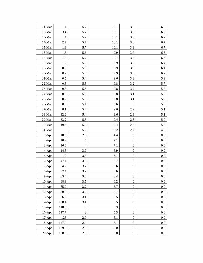
11-Mar 4 5.7 10.1 3.9 6.912-Mar 3.4 5.7 10.1 3.9 6.913-Mar 4 5.7 10.1 3.8 6.714-Mar 2.7 5.7 10.1 3.8 6.715-Mar 1.9 5.7 10.1 3.8 6.716-Mar 1.5 5.6 9.9 3.7 6.617-Mar 1.3 5.7 10.1 3.7 6.618-Mar 1.2 5.6 9.9 3.6 6.419-Mar 0.9 5.6 9.9 3.6 6.420-Mar 0.7 5.6 9.9 3.5 6.221-Mar 0.5 5.4 9.6 3.3 5.922-Mar 0.5 5.5 9.8 3.2 5.723-Mar 0.3 5.5 9.8 3.2 5.724-Mar 0.2 5.5 9.8 3.1 5.525-Mar 0.2 5.5 9.8 3.1 5.526-Mar 0.9 5.4 9.6 3 5.327-Mar 8.1 5.4 9.6 2.9 5.128-Mar 32.2 5.4 9.6 2.9 5.129-Mar 33.2 5.3 9.4 2.8 5.030-Mar 19.4 5.3 9.4 2.8 5.031-Mar 5.2 9.2 2.7 4.8
1-Apr 10.6 2.5 4.4 0 0.02-Apr 10.9 4 7.1 0 0.03-Apr 16.6 4 7.1 0 0.04-Apr 14.5 3.9 6.9 0 0.05-Apr 19 3.8 6.7 0 0.06-Apr 47.4 3.8 6.7 0 0.07-Apr 74.2 3.7 6.6 0 0.08-Apr 67.4 3.7 6.6 0 0.09-Apr 63.4 3.6 6.4 0 0.0
10-Apr 68.3 3.5 6.2 0 0.011-Apr 65.9 3.2 5.7 0 0.012-Apr 80.9 3.2 5.7 0 0.013-Apr 86.3 3.1 5.5 0 0.014-Apr 108.4 3.1 5.5 0 0.015-Apr 118.5 3 5.3 0 0.016-Apr 117.7 3 5.3 0 0.017-Apr 125 2.9 5.1 0 0.018-Apr 147.9 2.9 5.1 0 0.019-Apr 139.6 2.8 5.0 0 0.020-Apr 128.8 2.8 5.0 0 0.0

21-Apr 141.5 3.1 5.5 0 0.022-Apr 140.8 3.1 5.5 0 0.023-Apr 126.2 3 5.3 0 0.024-Apr 133.2 3 5.3 0 0.025-Apr 143.8 3 5.3 0 0.026-Apr 126.4 2.9 5.1 0 0.027-Apr 135.2 2.9 5.1 0 0.028-Apr 172.8 2.9 5.1 0 0.029-Apr 213.2 2.9 5.1 0 0.030-Apr 218.6 2.8 5.0 0 0.01-May 217.3 5.1 9.0 0.4 0.72-May 240.9 4.4 7.8 1.2 2.13-May 266.6 4.3 7.6 1.2 2.14-May 313.7 4.3 7.6 1.1 2.05-May 352.4 4.3 7.6 1.1 2.06-May 368.9 4.3 7.6 1.1 2.07-May 345.1 4.3 7.6 1.1 2.08-May 385.9 4.3 7.6 1.1 2.09-May 442.1 4.3 7.6 1.1 2.0
10-May 495.6 4.3 7.6 1.1 2.011-May 495.8 5.1 9.0 1.9 3.412-May 464.1 4.3 7.6 1.9 3.413-May 428.8 4.3 7.6 1.9 3.414-May 396.2 4.3 7.6 1.9 3.415-May 360.3 4.3 7.6 1.9 3.416-May 345.6 4.3 7.6 1.9 3.417-May 291.1 4.3 7.6 1.9 3.418-May 256.2 4.3 7.6 1.9 3.419-May 228.2 4.3 7.6 1.9 3.420-May 209 4.3 7.6 1.9 3.421-May 192.6 4.9 8.7 2.5 4.422-May 182.3 4.3 7.6 2.5 4.423-May 168.8 4.3 7.6 2.5 4.424-May 135.1 4.3 7.6 2.5 4.425-May 101.6 4.3 7.6 2.5 4.426-May 84 4.3 7.6 2.5 4.427-May 76.1 4.3 7.6 2.6 4.628-May 68.3 4.3 7.6 2.6 4.629-May 63 4.3 7.6 2.6 4.630-May 68.4 4.3 7.6 2.6 4.6