Volume 7 Algebras John Cannon Wieb Bosma Claus Fieker ... · HANDBOOK OF MAGMA FUNCTIONS Volume 7...
390
HANDBOOK OF MAGMA FUNCTIONS Volume 7 Algebras John Cannon Wieb Bosma Claus Fieker Allan Steel Editors Version 2.19 Sydney April 24, 2013
Transcript of Volume 7 Algebras John Cannon Wieb Bosma Claus Fieker ... · HANDBOOK OF MAGMA FUNCTIONS Volume 7...

HANDBOOK OF MAGMA FUNCTIONS
Volume 7
Algebras
John Cannon Wieb Bosma
Claus Fieker Allan Steel
Editors
Version 2.19
Sydney
April 24, 2013

ii

MAGMAC O M P U T E R • A L G E B R A
HANDBOOK OF MAGMA FUNCTIONS
Editors:
John Cannon Wieb Bosma Claus Fieker Allan Steel
Handbook Contributors:
Geoff Bailey, Wieb Bosma, Gavin Brown, Nils Bruin, John
Cannon, Jon Carlson, Scott Contini, Bruce Cox, Brendan
Creutz, Steve Donnelly, Tim Dokchitser, Willem de Graaf,
Andreas-Stephan Elsenhans, Claus Fieker, Damien Fisher,
Volker Gebhardt, Sergei Haller, Michael Harrison, Florian
Hess, Derek Holt, David Howden, Al Kasprzyk, Markus
Kirschmer, David Kohel, Axel Kohnert, Dimitri Leemans,
Paulette Lieby, Graham Matthews, Scott Murray, Eamonn
O’Brien, Dan Roozemond, Ben Smith, Bernd Souvignier,
William Stein, Allan Steel, Damien Stehle, Nicole Suther-
land, Don Taylor, Bill Unger, Alexa van der Waall, Paul
van Wamelen, Helena Verrill, John Voight, Mark Watkins,
Greg White
Production Editors:
Wieb Bosma Claus Fieker Allan Steel Nicole Sutherland
HTML Production:
Claus Fieker Allan Steel


VOLUME 7: OVERVIEW
XI ALGEBRAS . . . . . . . . . . . . . . . . . 241779 ALGEBRAS 241980 STRUCTURE CONSTANT ALGEBRAS 243181 ASSOCIATIVE ALGEBRAS 244182 FINITELY PRESENTED ALGEBRAS 246783 MATRIX ALGEBRAS 250584 GROUP ALGEBRAS 254585 BASIC ALGEBRAS 255986 QUATERNION ALGEBRAS 261987 ALGEBRAS WITH INVOLUTION 266388 CLIFFORD ALGEBRAS 2679
XII REPRESENTATION THEORY . . . . . . . . . 268389 MODULES OVER AN ALGEBRA 268590 K[G]-MODULES AND GROUP REPRESENTATIONS 272191 CHARACTERS OF FINITE GROUPS 275792 REPRESENTATIONS OF SYMMETRIC GROUPS 277993 MOD P GALOIS REPRESENTATIONS 2787

vi VOLUME 7: CONTENTS
VOLUME 7: CONTENTS
XI ALGEBRAS 2417
79 ALGEBRAS . . . . . . . . . . . . . . . . . . . . . . . 2419
79.1 Introduction 242179.1.1 The Categories of Algebras 242179.2 Construction of General Algebras and their Elements 242179.2.1 Construction of a General Algebra 242279.2.2 Construction of an Element of a General Algebra 242379.3 Construction of Subalgebras, Ideals and Quotient Algebras 242379.3.1 Subalgebras and Ideals 242379.3.2 Quotient Algebras 242479.4 Operations on Algebras and Subalgebras 242479.4.1 Invariants of an Algebra 242479.4.2 Changing Rings 242579.4.3 Bases 242579.4.4 Decomposition of an Algebra 242679.4.5 Operations on Subalgebras 242879.5 Operations on Elements of an Algebra 242979.5.1 Operations on Elements 242979.5.2 Comparisons and Membership 243079.5.3 Predicates on Elements 2430
80 STRUCTURE CONSTANT ALGEBRAS . . . . . . . . . . 2431
80.1 Introduction 243380.2 Construction of Structure Constant Algebras and Elements 243380.2.1 Construction of a Structure Constant Algebra 243380.2.2 Construction of Elements of a Structure Constant Algebra 243480.3 Operations on Structure Constant Algebras and Elements 243580.3.1 Operations on Structure Constant Algebras 243580.3.2 Indexing Elements 243680.3.3 The Module Structure of a Structure Constant Algebra 243780.3.4 Homomorphisms 2437
81 ASSOCIATIVE ALGEBRAS . . . . . . . . . . . . . . . . 2441
81.1 Introduction 244381.2 Construction of Associative Algebras 244381.2.1 Construction of an Associative Structure Constant Algebra 244381.2.2 Associative Structure Constant Algebras from other Algebras 244481.3 Operations on Algebras and their Elements 244581.3.1 Operations on Algebras 244581.3.2 Operations on Elements 244781.3.3 Representations 244881.3.4 Decomposition of an Algebra 244881.4 Orders 245081.4.1 Creation of Orders 245181.4.2 Attributes 245481.4.3 Bases of Orders 245581.4.4 Predicates 2456

VOLUME 7: CONTENTS vii
81.4.5 Operations with Orders 245781.5 Elements of Orders 245881.5.1 Creation of Elements 245881.5.2 Arithmetic of Elements 245881.5.3 Predicates on Elements 245981.5.4 Other Operations with Elements 245981.6 Ideals of Orders 246081.6.1 Creation of Ideals 246081.6.2 Attributes of Ideals 246181.6.3 Arithmetic for Ideals 246281.6.4 Predicates on Ideals 246281.6.5 Other Operations on Ideals 246381.7 Quaternionic Orders 246581.8 Bibliography 2466
82 FINITELY PRESENTED ALGEBRAS . . . . . . . . . . . 2467
82.1 Introduction 246982.2 Representation and Monomial Orders 246982.3 Exterior Algebras 247082.4 Creation of Free Algebras and Elements 247082.4.1 Creation of Free Algebras 247082.4.2 Print Names 247082.4.3 Creation of Polynomials 247182.5 Structure Operations 247182.5.1 Related Structures 247182.5.2 Numerical Invariants 247182.5.3 Homomorphisms 247282.6 Element Operations 247382.6.1 Arithmetic Operators 247382.6.2 Equality and Membership 247382.6.3 Predicates on Algebra Elements 247382.6.4 Coefficients, Monomials, Terms and Degree 247482.6.5 Evaluation 247682.7 Ideals and Grobner Bases 247782.7.1 Creation of Ideals 247782.7.2 Grobner Bases 247882.7.3 Verbosity 247982.7.4 Related Functions 248082.8 Basic Operations on Ideals 248282.8.1 Construction of New Ideals 248382.8.2 Ideal Predicates 248382.8.3 Operations on Elements of Ideals 248482.9 Changing Coefficient Ring 248582.10 Finitely Presented Algebras 248582.11 Creation of FP-Algebras 248582.12 Operations on FP-Algebras 248782.13 Finite Dimensional FP-Algebras 248882.14 Vector Enumeration 249282.14.1 Finitely Presented Modules 249282.14.2 S-algebras 249282.14.3 Finitely Presented Algebras 249382.14.4 Vector Enumeration 249382.14.5 The Isomorphism 249482.14.6 Sketch of the Algorithm 249582.14.7 Weights 2495

viii VOLUME 7: CONTENTS
82.14.8 Setup Functions 249682.14.9 The Quotient Module Function 249682.14.10 Structuring Presentations 249682.14.11 Options and Controls 249782.14.12 Weights 249782.14.13 Limits 249882.14.14 Logging 249982.14.15 Miscellaneous 2500
82.15 Bibliography 2503
83 MATRIX ALGEBRAS . . . . . . . . . . . . . . . . . . 2505
83.1 Introduction 2509
83.2 Construction of Matrix Algebras and their Elements 250983.2.1 Construction of the Complete Matrix Algebra 250983.2.2 Construction of a Matrix 250983.2.3 Constructing a General Matrix Algebra 251183.2.4 The Invariants of a Matrix Algebra 2512
83.3 Construction of Subalgebras, Ideals and Quotient Rings 2513
83.4 The Construction of Extensions and their Elements 251583.4.1 The Construction of Direct Sums and Tensor Products 251583.4.2 Construction of Direct Sums and Tensor Products of Elements 2517
83.5 Operations on Matrix Algebras 2518
83.6 Changing Rings 2518
83.7 Elementary Operations on Elements 251883.7.1 Arithmetic 251883.7.2 Predicates 2519
83.8 Elements of Mn as Homomorphisms 2523
83.9 Elementary Operations on Subalgebras and Ideals 252483.9.1 Bases 252483.9.2 Intersection of Subalgebras 252483.9.3 Membership and Equality 2524
83.10 Accessing and Modifying a Matrix 252583.10.1 Indexing 252583.10.2 Extracting and Inserting Blocks 252683.10.3 Joining Matrices 252683.10.4 Row and Column Operations 2527
83.11 Canonical Forms 252783.11.1 Canonical Forms for Matrices over Euclidean Domains 252783.11.2 Canonical Forms for Matrices over a Field 2529
83.12 Diagonalising Commutative Algebras over a Field 2532
83.13 Solutions of Systems of Linear Equations 2534
83.14 Presentations for Matrix Algebras 253583.14.1 Quotients and Idempotents 253583.14.2 Generators and Presentations 253883.14.3 Solving the Word Problem 2542
83.15 Bibliography 2544

VOLUME 7: CONTENTS ix
84 GROUP ALGEBRAS . . . . . . . . . . . . . . . . . . . 2545
84.1 Introduction 2547
84.2 Construction of Group Algebras and their Elements 254784.2.1 Construction of a Group Algebra 254784.2.2 Construction of a Group Algebra Element 2549
84.3 Construction of Subalgebras, Ideals and Quotient Algebras 2550
84.4 Operations on Group Algebras and their Subalgebras 255284.4.1 Operations on Group Algebras 255284.4.2 Operations on Subalgebras of Group Algebras 2553
84.5 Operations on Elements 2555
85 BASIC ALGEBRAS . . . . . . . . . . . . . . . . . . . 2559
85.1 Introduction 2563
85.2 Basic Algebras 256385.2.1 Creation 256385.2.2 Special Basic Algebras 256485.2.3 Access Functions 257085.2.4 Elementary Operations 257185.2.5 Boolean Functions 2575
85.3 Homomorphisms 2575
85.4 Subalgebras and Quotient Algebras 257685.4.1 Subalgebras and their Constructions 257685.4.2 Ideals and their Construction 257785.4.3 Quotient Algebras 2578
85.5 Minimal Forms and Gradings 2579
85.6 Automorphisms and Isomorphisms 2581
85.7 Modules over Basic Algebras 258385.7.1 Indecomposable Projective Modules 258385.7.2 Creation 258485.7.3 Access Functions 258585.7.4 Predicates 258785.7.5 Elementary Operations 2588
85.8 Homomorphisms of Modules 259085.8.1 Creation 259085.8.2 Access Functions 259185.8.3 Projective Covers and Resolutions 2592
85.9 Duals and Injectives 259685.9.1 Injective Modules 2597
85.10 Cohomology 260085.10.1 Ext-Algebras 2605
85.11 Group Algebras of p-groups 260785.11.1 Access Functions 260885.11.2 Projective Resolutions 260885.11.3 Cohomology Generators 260985.11.4 Cohomology Rings 261085.11.5 Restrictions and Inflations 2610
85.12 A-infinity Algebra Structures on Group Cohomology 261485.12.1 Homological Algebra Toolkit 2616
85.13 Bibliography 2618

x VOLUME 7: CONTENTS
86 QUATERNION ALGEBRAS . . . . . . . . . . . . . . . . 2619
86.1 Introduction 262186.2 Creation of Quaternion Algebras 262286.3 Creation of Quaternion Orders 262686.3.1 Creation of Orders from Elements 262786.3.2 Creation of Maximal Orders 262886.3.3 Creation of Orders with given Discriminant 263086.3.4 Creation of Orders with given Discriminant over the Integers 263186.4 Elements of Quaternion Algebras 263286.4.1 Creation of Elements 263286.4.2 Arithmetic of Elements 263286.5 Attributes of Quaternion Algebras 263486.6 Hilbert Symbols and Embeddings 263686.7 Predicates on Algebras 263986.8 Recognition Functions 264086.9 Attributes of Orders 264286.10 Predicates of Orders 264386.11 Operations with Orders 264486.12 Ideal Theory of Orders 264586.12.1 Creation and Access Functions 264586.12.2 Enumeration of Ideal Classes 264886.12.3 Operations on Ideals 265186.13 Norm Spaces and Basis Reduction 265286.14 Isomorphisms 265486.14.1 Isomorphisms of Algebras 265486.14.2 Isomorphisms of Orders 265586.14.3 Isomorphisms of Ideals 265586.14.4 Examples 265786.15 Units and Unit Groups 265986.16 Bibliography 2661
87 ALGEBRAS WITH INVOLUTION . . . . . . . . . . . . . 2663
87.1 Introduction 266587.2 Algebras with Involution 266587.2.1 Reflexive Forms 266687.2.2 Systems of Reflexive Forms 266687.2.3 Basic Attributes of ∗-Algebras 266787.2.4 Adjoint Algebras 266887.2.5 Group Algebras 266987.2.6 Simple ∗-Algebras 267087.3 Decompositions of ∗-Algebras 267187.4 Recognition of ∗-Algebras 267287.4.1 Recognition of Simple ∗-Algebras 267287.4.2 Recognition of Arbitrary ∗-Algebras 267387.5 Intersections of Classical Groups 267587.6 Bibliography 2677
88 CLIFFORD ALGEBRAS . . . . . . . . . . . . . . . . . 2679
88.1 Introduction 268188.2 Clifford Algebras and their Elements 268188.2.1 Elements of a Clifford Algebra 268288.3 Bibliography 2682

VOLUME 7: CONTENTS xi
XII REPRESENTATION THEORY 2683
89 MODULES OVER AN ALGEBRA . . . . . . . . . . . . . 2685
89.1 Introduction 2687
89.2 Modules over a Matrix Algebra 268889.2.1 Construction of an A-Module 268889.2.2 Accessing Module Information 268989.2.3 Standard Constructions 269189.2.4 Element Construction and Operations 269289.2.5 Submodules 269489.2.6 Quotient Modules 269789.2.7 Structure of a Module 269889.2.8 Decomposability and Complements 270489.2.9 Lattice of Submodules 270689.2.10 Homomorphisms 2710
89.3 Modules over a General Algebra 271689.3.1 Introduction 271689.3.2 Construction of Algebra Modules 271689.3.3 The Action of an Algebra Element 271789.3.4 Related Structures of an Algebra Module 271789.3.5 Properties of an Algebra Module 271889.3.6 Creation of Algebra Modules from other Algebra Modules 2718
90 K[G]-MODULES AND GROUP REPRESENTATIONS . . . . 2721
90.1 Introduction 2723
90.2 Construction of K[G]-Modules 272390.2.1 General K[G]-Modules 272390.2.2 Natural K[G]-Modules 272590.2.3 Action on an Elementary Abelian Section 272690.2.4 Permutation Modules 272790.2.5 Action on a Polynomial Ring 2729
90.3 The Representation Afforded by a K[G]-module 2730
90.4 Standard Constructions 273290.4.1 Changing the Coefficient Ring 273290.4.2 Writing a Module over a Smaller Field 273390.4.3 Direct Sum 273790.4.4 Tensor Products of K[G]-Modules 273790.4.5 Induction and Restriction 273890.4.6 The Fixed-point Space of a Module 273990.4.7 Changing Basis 2739
90.5 The Construction of all Irreducible Modules 274090.5.1 Generic Functions for Finding Irreducible Modules 274090.5.2 The Burnside Algorithm 274390.5.3 The Schur Algorithm for Soluble Groups 274490.5.4 The Rational Algorithm 2747
90.6 Extensions of Modules 2750
90.7 The Construction of Projective Indecomposable Modules 2751

xii VOLUME 7: CONTENTS
91 CHARACTERS OF FINITE GROUPS . . . . . . . . . . . 2757
91.1 Creation Functions 275991.1.1 Structure Creation 275991.1.2 Element Creation 275991.1.3 The Table of Irreducible Characters 276091.2 Character Ring Operations 276491.2.1 Related Structures 276491.3 Element Operations 276591.3.1 Arithmetic 276591.3.2 Predicates and Booleans 276591.3.3 Accessing Class Functions 276691.3.4 Conjugation of Class Functions 276791.3.5 Functions Returning a Scalar 276791.3.6 The Schur Index 276891.3.7 Attribute 277191.3.8 Induction, Restriction and Lifting 277191.3.9 Symmetrization 277291.3.10 Permutation Character 277391.3.11 Composition and Decomposition 277391.3.12 Finding Irreducibles 277391.3.13 Brauer Characters 277691.4 Bibliography 2778
92 REPRESENTATIONS OF SYMMETRIC GROUPS . . . . . . 2779
92.1 Introduction 278192.2 Representations of the Symmetric Group 278192.2.1 Integral Representations 278192.2.2 The Seminormal and Orthogonal Representations 278292.3 Characters of the Symmetric Group 278392.3.1 Single Values 278392.3.2 Irreducible Characters 278392.3.3 Character Table 278392.4 Representations of the Alternating Group 278392.5 Characters of the Alternating Group 278492.5.1 Single Values 278492.5.2 Irreducible Characters 278492.5.3 Character Table 278492.6 Bibliography 2785
93 MOD P GALOIS REPRESENTATIONS . . . . . . . . . . . 2787
93.1 Introduction 278993.1.1 Motivation 278993.1.2 Definitions 278993.1.3 Classification of ϕ-modules 279093.1.4 Connection with Galois Representations 279093.2 ϕ-modules and Galois Representations in Magma 279093.2.1 ϕ-modules 279193.2.2 Semisimple Galois Representations 279293.3 Examples 2793

PART XIALGEBRAS
79 ALGEBRAS 2419
80 STRUCTURE CONSTANT ALGEBRAS 2431
81 ASSOCIATIVE ALGEBRAS 2441
82 FINITELY PRESENTED ALGEBRAS 2467
83 MATRIX ALGEBRAS 2505
84 GROUP ALGEBRAS 2545
85 BASIC ALGEBRAS 2559
86 QUATERNION ALGEBRAS 2619
87 ALGEBRAS WITH INVOLUTION 2663
88 CLIFFORD ALGEBRAS 2679


79 ALGEBRAS79.1 Introduction . . . . . . . . 2421
79.1.1 The Categories of Algebras . . . . 2421
79.2 Construction of GeneralAlgebras and their Elements . 2421
79.2.1 Construction of a General Algebra . 2422
Algebra< > 2422AssociativeAlgebra< > 2422QuaternionAlgebra< > 2422LieAlgebra< > 2422LieAlgebra(A) 2422GroupAlgebra(R, G) 2422MatrixAlgebra(R, n) 2422
79.2.2 Construction of an Element of a Gen-eral Algebra . . . . . . . . . . 2423
Zero(A) 2423! 2423One(A) 2423! 2423Random(A) 2423
79.3 Construction of Subalgebras,Ideals and Quotient Algebras . 2423
79.3.1 Subalgebras and Ideals . . . . . . 2423
sub< > 2423lideal< > 2423rideal< > 2424ideal< > 2424
79.3.2 Quotient Algebras . . . . . . . . 2424
quo< > 2424/ 2424
79.4 Operations on Algebras and Sub-algebras . . . . . . . . . . 2424
79.4.1 Invariants of an Algebra . . . . . 2424
CoefficientRing(A) 2424BaseRing(A) 2424Dimension(A) 2424# 2424
79.4.2 Changing Rings . . . . . . . . . 2425
ChangeRing(A, S) 2425ChangeRing(A, S, f) 2425
79.4.3 Bases . . . . . . . . . . . . . 2425
BasisElement(A, i) 2425. 2425Basis(A) 2425IsIndependent(Q) 2425ExtendBasis(S, A) 2425ExtendBasis(Q, A) 2425
79.4.4 Decomposition of an Algebra . . . 2426
CompositionSeries(A) 2426CompositionFactors(A) 2426MinimalLeftIdeals(A : -) 2426MinimalRightIdeals(A : -) 2426MinimalIdeals(A : -) 2426MaximalLeftIdeals(A : -) 2426MaximalRightIdeals(A : -) 2426MaximalIdeals(A : -) 2426JacobsonRadical(A) 2426IsSemisimple(A) 2427IsSimple(A) 2427
79.4.5 Operations on Subalgebras . . . . 2428
IsZero(A) 2428eq 2428ne 2428subset 2428notsubset 2428meet 2428* 2428^ 2428Morphism(A, B) 2428
79.5 Operations on Elements of an Al-gebra . . . . . . . . . . . 2429
79.5.1 Operations on Elements . . . . . 2429
+ 2429- 2429- 2429* 2429* 2429* 2429/ 2429^ 2429MinimalPolynomial(a) 2429Parent(a) 2429
79.5.2 Comparisons and Membership . . 2430
eq 2430ne 2430in 2430notin 2430
79.5.3 Predicates on Elements . . . . . 2430
IsZero(a) 2430IsOne(a) 2430IsMinusOne(a) 2430IsUnit(a) 2430IsRegular(a) 2430IsZeroDivisor(a) 2430IsIdempotent(a) 2430IsNilpotent(a) 2430


Chapter 79
ALGEBRAS
79.1 Introduction
Algebras are viewed as free modules over a ring R with an additional multiplication. Thereare no a priori conditions imposed on the ring except that it must be unital, but somefunctions may require that an echelonization algorithm is available for modules over R andsometimes it is also required that R is a field. For example, quotients of algebras can onlybe constructed over fields, since otherwise the quotient module is not necessarily a freemodule over R.
The most general way to define an algebra is by structure constants, but for specialtypes of algebras Magma uses more efficient representations.
79.1.1 The Categories of AlgebrasAt present, Magma contains seven main categories of algebras:
(1)General algebras represented by structure constants: category AlgGen;
(2)Associative algebras represented by structure constants: category AlgAss;
(3)Quaternion algebras as special types of associative algebras; category AlgQuat;
(4)Lie algebras represented by structure constants: category AlgLie;
(5)Group algebras: category AlgGrp with a special type AlgGrpSub for subalgebras ofgroup algebras;
(6)Matrix algebras: category AlgMat;
(7)Finitely presented algebras: category AlgFP.
The hierarchy of these categories is such that AlgGen is on the top level and AlgAss andAlgLie are on the next level inheriting the functions available for AlgGen. The categoriesAlgQuat, AlgGrp and AlgMat are on a third level inheriting the functions available forAlgAss. Finitely presented algebras are independent of the other categories.
79.2 Construction of General Algebras and their Elements

2422 ALGEBRAS Part XII
79.2.1 Construction of a General AlgebraThe construction of an algebra depends on its category. The chapters on the individualalgebra categories describe this in detail. Here only an overview is given.
Algebra< R, n | Q >
Let R be ring, n an integer and Q a sequence of n3 elements of R. This functioncreates an algebra A of dimension n over R with basis e1, . . . , en such that Q containsthe structure constants of A, i.e. ei∗ej =
∑ak
ijek, where akij is the element in position
(i− 1) ∗ n2 + (j − 1) ∗ n+ k of Q.
AssociativeAlgebra< R, n | Q >
Check BoolElt Default : true
This function creates the associative structure constant algebra A as returned byAlgebra< R, n | Q >. By default, the algebra is checked on associativity, but thiscan be avoided by setting Check := false. The returned algebra is of type AlgAss.
QuaternionAlgebra< K | a, b >
This function creates the quaternion algebra A over the field K on generators x andy with relations x2 = a, y2 = b, and xy = −yx.
LieAlgebra< R, n | Q >
Check BoolElt Default : true
This function creates the Lie structure constant algebra A as returned by Algebra<R, n | Q >. By default, the algebra is checked to be a Lie algebra, but this can beavoided by setting Check := false. The returned algebra is of type AlgLie.
LieAlgebra(A)
Given an associative algebra A, create the Lie algebra generated by the elements inL using the induced Lie product (x, y) → x ∗ y − y ∗ x.
GroupAlgebra(R, G)
Given a ring R and a group G construct the group algebra R[G] of dimension |G|over R.
MatrixAlgebra(R, n)
Given a positive integer n and a ring R, create the full matrix algebra Mn(R) ofdimension n2 over R.

Ch. 79 ALGEBRAS 2423
79.2.2 Construction of an Element of a General AlgebraThe construction of a generic element of an algebra varies for the different types of algebrasand is therefore explained in the corresponding chapters.
Zero(A)
A ! 0
Create the zero element of the algebra A.
One(A)
A ! 1
If it exists, create the identity element of the algebra A; otherwise an error occurs.
Random(A)
Given an algebra A defined over a finite ring, return a random element.
79.3 Construction of Subalgebras, Ideals and Quotient Algebras
79.3.1 Subalgebras and IdealsIf the coefficient ring R of an algebra A is a Euclidean domain then one may constructsubmodules and ideals of A in Magma.
sub< A | L >
Create the subalgebra S of the algebra A that is generated by the elements definedby L, where L is a list of one or more items of the following types:(a)An element of A;(b)A set or sequence of elements of A;(c) A subalgebra or ideal of A;(d)A set or sequence of subalgebras or ideals of A.The constructor returns the subalgebra as an algebra of the same type as A. Anexception are group algebras, where the subalgebra is either of type AlgAss or of thespecial type AlgGrpSub. As well as the subalgebra S itself, the constructor returnsthe inclusion homomorphism f : S → A.
lideal< A | L >
Create the left ideal I of the algebra A generated by the elements defined by L,where L is a list as for the sub constructor above.
The constructor returns the left ideal as an algebra of the same type as A withthe same exception for group algebras as for the sub constructor. As well as the leftideal I itself, the constructor returns the inclusion homomorphism f : I → A.

2424 ALGEBRAS Part XII
rideal< A | L >
Create the right ideal I of the algebra A generated by the elements defined by L,where L is a list as for the sub constructor above.
The constructor returns the right ideal as an algebra of the same type as A withthe same exception for group algebras as for the sub constructor. As well as theright ideal I itself, the constructor returns the inclusion homomorphism f : I → A.
ideal< A | L >
Create the (two-sided) ideal I of the algebra A generated by the elements definedby L, where L is a list as for the sub constructor above.
The constructor returns the right ideal as an algebra of the same type as A withthe same exception for group algebras as for the sub constructor. As well as theideal I itself, the constructor returns the inclusion homomorphism f : I → A.
79.3.2 Quotient AlgebrasIf the coefficient ring R of an algebra A is a field, then quotient algebras of A may also beconstructed.
quo< A | L >
Create the quotient algebra Q = A/I, where I is the two-sided ideal of A generatedby the elements of A specified by the list L, which should satisfy the same conditionsas for the sub constructor above.
The constructor returns the quotient as a structure constant algebra with degreeequal to its dimension. If A is known to be associative, then Q is of type AlgAss,otherwise Q is of type AlgGen. As well as the quotient Q itself, the constructorreturns the natural homomorphism f : A→ Q.
A / S
The quotient of the algebra A by the (two-sided) ideal closure of its subalgebra S.
79.4 Operations on Algebras and Subalgebras
79.4.1 Invariants of an Algebra
CoefficientRing(A)
BaseRing(A)
The coefficient ring (or base ring) over which the algebra A is defined.
Dimension(A)
The dimension of the algebra A.
#A
The cardinality of the algebra A if both R and the dimension of A are finite. Notethat this cannot be computed if the dimension of A is too large.

Ch. 79 ALGEBRAS 2425
79.4.2 Changing Rings
ChangeRing(A, S)
Given an algebra A with base ring R, together with a ring S, construct the algebraB with base ring S obtained by coercing the coefficients of elements of A into S,together with the homomorphism from A to B.
This function can not be applied if A is of type AlgGrpSub, as the parent structureof elements of A is the full group algebra of which A is a subalgebra.
ChangeRing(A, S, f)
Given an algebra A with base ring R, together with a ring S and a map f : R→ S,construct the algebra B with base ring S obtained by mapping the coefficients ofelements of A into S via f , together with the homomorphism from A to B.
As above, this function can not be applied if A is of type AlgGrpSub.
79.4.3 BasesIn general, every algebra comes with a basis, corresponding to its underlying modulestructure. The only exception for that are group algebras in the "Terms" representation,where the dimension of the algebra may be too large to create vectors of that degree.
BasisElement(A, i)
A . i
The i-th basis element of the algebra A.
Basis(A)
The basis of the algebra A, as a sequence of elements of A.Note that if A is of type AlgGrpSub the returned elements will be elements of
the full group algebra of which A is a subalgebra.
IsIndependent(Q)
Given a sequence Q of elements of the R-algebra A, this functions returns true ifthese elements are linearly independent over R; otherwise false.
ExtendBasis(S, A)
ExtendBasis(Q, A)
Given an algebra A and either a subalgebra S of dimension m of A or a sequenceQ of m linearly independent elements of A, return a sequence containing a basis ofA such that the first m elements are the basis of S resp. the elements in Q.

2426 ALGEBRAS Part XII
79.4.4 Decomposition of an AlgebraAn algebra A can be regarded as a (left- or right-) module for itself. If A is defined over afinite field, the machinery to decompose modules over finite fields can be used to investigatethe structure of the algebra A.
CompositionSeries(A)
Compute a composition series for the algebra A. The function has three returnvalues:(a) a sequence containing the composition series as an ascending chain of subalgebras
such that the successive quotients are irreducible A-modules;(b)a sequence containing the composition factors as structure constant algebras;(c) a transformation matrix to a basis compatible with the composition series, that
is, the first basis elements form a basis of the first term of the composition series,the next extend these to a basis for the second term etc.
CompositionFactors(A)
Compute the composition factors of a composition series for the algebra A. Thisfunction returns the same as the second return value of CompositionSeries above,but will often be very much quicker.
MinimalLeftIdeals(A : parameters)
MinimalRightIdeals(A : parameters)
MinimalIdeals(A : parameters)
Limit RngIntElt Default : ∞Return the minimal left/right/two-sided ideals of A (in non-decreasing size). IfLimit is set to n, at most n ideals are calculated and the second return valueindicates whether all of the ideals were computed.
MaximalLeftIdeals(A : parameters)
MaximalRightIdeals(A : parameters)
MaximalIdeals(A : parameters)
Limit RngIntElt Default : ∞Return the maximal left/right/two-sided ideals of A (in non-decreasing size). IfLimit is set to n, at most n ideals are calculated and the second return valueindicates whether all of the ideals were computed.
JacobsonRadical(A)
Construct the Jacobson (or nilpotent) radical of A, that is, the intersection of themaximal ideals of A (which is equal to the intersection of the maximal left or rightideals).

Ch. 79 ALGEBRAS 2427
IsSemisimple(A)
Return true if the Jacobson radical of A is trivial; otherwise false.
IsSimple(A)
Return true if A has no non-trivial composition factor; otherwise false.
Example H79E1
We create a division algebra of dimension 4 over the rational field.
> Q := MatrixAlgebra< Rationals(), 4 |
> [0,1,0,0, -1,0,0,0, 0,0,0,-1, 0,0,1,0],
> [0,0,1,0, 0,0,0,1, -1,0,0,0, 0,-1,0,0]>;
> i := Q.1;
> j := Q.2;
> k := i*j;
> Dimension(Q);
4
> MinimalPolynomial( (1+i+j+k)/2 );
$.1^2 - $.1 + 1
Hence, the element (1+i+j+k)/2 is integral. In fact, together with 1, i and j it forms a Z-basisof a maximal order in Q. We create this maximal order as a structure constant algebra over theintegers.
> a := [ Q!1, i, j, (1+i+j+k)/2 ];
> T := MatrixAlgebra(Rationals(),4) ! &cat[ Coordinates(Q,a[i]) : i in [1..4] ];
> V := RSpace(Rationals(), 4);
> C := [ V ! Coordinates(Q, a[i]*a[j]) * T^-1 : j in [1..4], i in [1..4] ];
> A := ChangeRing( Algebra< V | C >, Integers() );
> IsAssociative(A);
true
> AA := AssociativeAlgebra(A);
> AA;
Associative Algebra of dimension 4 with base ring Integer Ring
> MinimalPolynomial(AA.4);
$.1^2 - $.1 + 1
The so constructed maximal order is ramified at 2 and ∞, hence it should be simple after reducingat odd primes.
> for p in [ i : i in [1..100] | IsPrime(i) ] do
> if not IsSimple( ChangeRing( AA, GF(p) ) ) then
> print p;
> end if;
> end for;
2
> CS, CF, T := CompositionSeries( ChangeRing( AA, GF(2) ) );
> T;
[1 0 1 0]

2428 ALGEBRAS Part XII
[0 1 1 0]
[0 0 1 0]
[0 0 0 1]
A glance at the preimages of the basis of the irreducible submodule shows the ramification of AAat the prime 2.
> MinimalPolynomial(AA.1 + AA.3);
$.1^2 - 2*$.1 + 2
> MinimalPolynomial(AA.2 + AA.3);
$.1^2 + 2
79.4.5 Operations on Subalgebras
IsZero(A)
Returns true if the algebra A is trivial; otherwise false.
A eq B
Returns true if the algebras A and B (having a common superalgebra) are equal;otherwise false.
A ne B
Returns true if the algebras A and B are not equal; otherwise false.
A subset B
Returns true if A is a subalgebra of the algebra B; otherwise false.
A notsubset B
Returns true if A is not a subalgebra of the algebra B; otherwise false.
A meet B
The intersection of the algebras A and B, which must have a common superalgebra.
A * B
The algebra product A ∗ B of the algebras A and B, which must have a commonsuperalgebra.
A ^ n
The (left-normed) n-th power of the algebra A, i.e. ((. . . (A ∗A) ∗ . . .) ∗A).
Morphism(A, B)
The map giving the morphism from A to B. Either A is a subalgebra of B, in whichcase the embedding of A into B is returned, or B is a quotient algebra of A, inwhich case the natural epimorphism from A onto B is returned.

Ch. 79 ALGEBRAS 2429
79.5 Operations on Elements of an Algebra
79.5.1 Operations on Elements
a + b
The sum of the elements a and b of an algebra A.
-a
The negation of the algebra element a.
a - b
The difference of the elements a and b of an algebra A.
a * b
The product of the elements a and b of an algebra A.
a * r
r * a
The product of the element a of the algebra A and the ring element r ∈ R, whereR is the coefficient ring of A.
a / r
The product of the element a of the R-algebra A and the ring element 1/r ∈ R,where R is a field.
a ^ n
If n is positive, form the (left-normed) n-th power ((. . . ((a ∗ a) ∗ a) . . .) ∗ a) of a; ifthe parent algebra A of a has an identity and n is zero, return the identity; if n < 0and a has an inverse a−1 in A, form the n-th power of a−1.
MinimalPolynomial(a)
If R is a field or the integer ring, return the minimal polynomial of the algebraelement a.
Parent(a)
For an element a in an algebra A return A.

2430 ALGEBRAS Part XII
79.5.2 Comparisons and Membership
a eq b
Returns true if the elements a and b of an algebra A are equal; otherwise false.
a ne b
Returns true if the elements a and b of an algebra A are not equal; otherwise false.
a in A
Returns true if a is in the algebra A; otherwise false.
a notin A
Returns true if a is not in the algebra A; otherwise false.
79.5.3 Predicates on Elements
IsZero(a)
Returns true if the algebra element a is zero; otherwise false.
IsOne(a)
Returns true if the algebra element a is the identity; otherwise false.
IsMinusOne(a)
Returns true if the algebra element a is the negative of the identity element; oth-erwise false.
IsUnit(a)
Returns true if the element a is a unit, plus the inverse; otherwise false.
IsRegular(a)
Returns true if the element a is regular, that is, is not a zero divisor; otherwisefalse.
IsZeroDivisor(a)
Returns true if the algebra element a is a divisor of zero; otherwise false.
IsIdempotent(a)
Returns true if the element a is an idempotent, i.e. if a2 = a; otherwise false.
IsNilpotent(a)
Returns true if the element a is nilpotent, i.e. if an = 0 for some n ≥ 0; otherwisefalse. If true, the minimal n such that an = 0 is returned as a second value.

80 STRUCTURE CONSTANT ALGEBRAS80.1 Introduction . . . . . . . . 2433
80.2 Construction of Structure Con-stant Algebras and Elements . 2433
80.2.1 Construction of a Structure ConstantAlgebra . . . . . . . . . . . . 2433
Algebra< > 2433Algebra< > 2433Algebra< > 2434ChangeBasis(A, B) 2434ChangeBasis(A, B) 2434ChangeBasis(A, B) 2434
80.2.2 Construction of Elements of a Struc-ture Constant Algebra . . . . . . 2434
elt< > 2434! 2434BasisProduct(A, i, j) 2434BasisProducts(A) 2435
80.3 Operations on StructureConstant Algebras and Elements2435
80.3.1 Operations on Structure ConstantAlgebras . . . . . . . . . . . . 2435
IsCommutative(A) 2435IsAssociative(A) 2435IsLie(A) 2435DirectSum(A, B) 2435
80.3.2 Indexing Elements . . . . . . . . 2436
a[i] 2436a[i] := r 2436
80.3.3 The Module Structure of a StructureConstant Algebra . . . . . . . . 2437
Module(A) 2437Degree(A) 2437Degree(a) 2437ElementToSequence(a) 2437Eltseq(a) 2437Coordinates(S, a) 2437InnerProduct(a, b) 2437Support(a) 2437
80.3.4 Homomorphisms . . . . . . . . 2437
hom< > 2437


Chapter 80
STRUCTURE CONSTANT ALGEBRAS
80.1 IntroductionA structure constant algebra A of dimension n over a ring R can be defined in Magma bygiving the n3 structure constants ak
ij ∈ R(1 ≤ i, j, k ≤ n) such that, if e1, e2, . . . , en is thebasis of A, ei ∗ ej =
∑nk=1 a
kij ∗ ek. Structure constant algebras may be defined over any
unital ring R. However, many operations require that R be a Euclidean domain or even afield.
80.2 Construction of Structure Constant Algebras and Elements
80.2.1 Construction of a Structure Constant AlgebraThere are three ways in Magma to specify the structure constants for a structure constantalgebra A of dimension n. The first is to give n3 ring elements, the second to identify Awith the module M = Rn and give the products ei ∗ ej as elements of M and the third tospecify only the non-zero structure constants.
Algebra< R, n | Q : parameters >
Algebra< M | Q : parameters >
Rep MonStgElt Default : “Dense”This function creates the structure constant algebra A over the free moduleM = Rn,with standard basis e1, e2, . . . , en, and with the structure constants ak
ij being givenby the sequence Q. The sequence Q can be of any of the following three forms. Notethat in all cases the actual ordering of the structure constants is the same: it is onlytheir division that varies.(i) A sequence of n sequences of n sequences of length n. The j-th element of the
i-th sequence is the sequence [a1ij , . . . , a
nij ], or the element (a1
ij , . . . , anij) of M ,
giving the coefficients of the product ei ∗ ej .(ii)A sequence of n2 sequences of length n, or n2 elements ofM . Here the coefficients
of ei ∗ ej are given by position (i− 1) ∗ n+ j of Q.(iii)A sequence of n3 elements of the ringR. Here the sequence elements are the struc-
ture constants themselves, with the ordering a111, a
211, . . . , a
n11, a
112, a
212, . . . , a
nnn.
So akij lies in position (i− 1) ∗ n2 + (j − 1) ∗ n+ k of Q.
The optional parameter Rep can be used to select the internal representation ofthe structure constants. The possible values for Rep are "Dense", "Sparse" and"Partial", with the default being "Dense". In the dense format, the n3 structure

2434 ALGEBRAS Part XII
constants are stored as n2 vectors of length n, similarly to (ii) above. This is the bestrepresentation if most of the structure constants are non-zero. The sparse format,intended for use when most structure constants are zero, stores the positions andvalues of the non-zero structure constants. The partial format stores the vectors,but records for efficiency the positions of the non-zero structure constants.
Algebra< R, n | T : parameters >
Rep MonStgElt Default : “Sparse”
This function creates the structure constant algebra A with standard basise1, e2, . . . , en over R. The sequence T contains quadruples < i, j, k, ak
ij > givingthe non-zero structure constants. All other structure constants are defined to be 0.
As above, the optional parameter Rep can be used to select the internal repre-sentation of the structure constants.
ChangeBasis(A, B)
ChangeBasis(A, B)
ChangeBasis(A, B)
Rep MonStgElt Default : “Dense”
Create a new structure constant algebra A′, isomorphic to A, by recomputing thestructure constants with respect to the basis B. The basis B can be specified asa set or sequence of elements of A, a set or sequence of vectors, or a matrix. Thesecond returned value is the isomorphism from A to A′.
As above, the optional parameter Rep can be used to select the internal repre-sentation of the structure constants. Note that the default is dense representation,regardless of the representation used by A.
80.2.2 Construction of Elements of a Structure Constant Algebra
elt< A | r1, r2, . . . , rn >
Given a structure constant algebra A of dimension n over a ring R, and ring elementsr1, r2, . . . , rn ∈ R construct the element r1 ∗ e1 + r2 ∗ e2 + . . .+ rn ∗ en of A.
A ! Q
Given a structure constant algebra A of dimension n and a sequence Q =[r1, r2, . . . , rn] of elements of the base ring R of A, construct the element r1 ∗ e1 +r2 ∗ e2 + . . .+ rn ∗ en of A.
BasisProduct(A, i, j)
Return the product of the i-th and j-th basis element of the algebra A.

Ch. 80 STRUCTURE CONSTANT ALGEBRAS 2435
BasisProducts(A)
Rep MonStgElt Default : “Dense”
Return the products of all basis elements of the algebra A.The optional parameter Rep may be used to specify the format of the result. If
Rep is set to “Dense”, the products are returned as a sequence Q of n sequences ofn elements of A, where n is the dimension of A. The element Q[i][j] is the productof the i-th and j-th basis elements.
If Rep is set to “Sparse”, the products are returned as a sequence Q contain-ing quadruples (i, j, k, aijk) signifying that the product of the i-th and j-th basiselements is
∑nk=1 aijkbk, where bk is the k-th basis element and n = dim(A).
80.3 Operations on Structure Constant Algebras and Elements
80.3.1 Operations on Structure Constant Algebras
IsCommutative(A)
Returns true if the algebra A is commutative; otherwise false.
IsAssociative(A)
Returns true if the algebra A is associative; otherwise false.Note that for a structure constant algebra of dimension n this requires up to n3
tests.
IsLie(A)
Returns true if the algebra A is a Lie algebra; otherwise false.Note that for a structure constant algebra of dimension n this requires about
n3/3 tests of the Jacobi identity.
DirectSum(A, B)
Construct a structure constant algebra of dimension n+m where n and m are thedimensions of the algebras A and B, respectively. The basis of the new algebra isthe concatenation of the bases of A and B and the products a ∗ b where a ∈ A andb ∈ B are defined to be 0.

2436 ALGEBRAS Part XII
Example H80E1
We define a structure constant algebra which is a Jordan algebra.
> M := MatrixAlgebra( GF(3), 2 );
> B := Basis(M);
> C := &cat[Coordinates(M,(B[i]*B[j]+B[j]*B[i])/2) : j in [1..#B], i in [1..#B]];
> A := Algebra< GF(3), #B | C >;
> #A;
81
> IsAssociative(A);
false
> IsLie(A);
false
> IsCommutative(A);
true
This is a good start, as one of the defining properties of Jordan algebras is that they are commu-tative. The other property is that the identity (x2 ∗ y) ∗ x = x2 ∗ (y ∗ x) holds for all x, y ∈ A. Wecheck this on a random pair.
> x := Random(A); y := Random(A); print (x^2*y)*x - x^2*(y*x);
(0 0 0 0)
The algebra is small enough to check this identity on all elements.
> forall<x, y>: x, y in A | (x^2*y)*x eq x^2*(y*x);
true
So the algebra is in fact a Jordan algebra (which was clear by construction). We finally have alook at the structure constants.
> BasisProducts(A);
[
[ (1 0 0 0), (0 2 0 0), (0 0 2 0), (0 0 0 0) ],
[ (0 2 0 0), (0 0 0 0), (2 0 0 2), (0 2 0 0) ],
[ (0 0 2 0), (2 0 0 2), (0 0 0 0), (0 0 2 0) ],
[ (0 0 0 0), (0 2 0 0), (0 0 2 0), (0 0 0 1) ]
]
80.3.2 Indexing Elements
a[i]
If a is an element of a structure constant algebra A of dimension n and 1 ≤ i ≤ nis a positive integer, then the i-th component of the element a is returned (as anelement of the base ring R of A).
a[i] := r
Given an element a belonging to a structure constant algebra of dimension n overR, a positive integer 1 ≤ i ≤ n and an element r ∈ R, the i-th component of theelement a is redefined to be r.

Ch. 80 STRUCTURE CONSTANT ALGEBRAS 2437
80.3.3 The Module Structure of a Structure Constant Algebra
Module(A)
The module Rn underlying the structure constant algebra A.
Degree(A)
The degree (= dimension) of the module underlying the algebra A.
Degree(a)
Given an element belonging to the structure constant algebra A of dimension n,return n.
ElementToSequence(a)
Eltseq(a)
The sequence of coefficients of the structure constant algebra element a.
Coordinates(S, a)
Let a be an element of a structure constant algebra A and let S be a subalgebra ofA containing a. This function returns the coefficients of a with respect to the basisof S.
InnerProduct(a, b)
The (Euclidean) inner product of the coefficient vectors of a and b, where a and bare elements of some structure constant algebra A.
Support(a)
The support of the structure constant algebra element a; i.e. the set of indices ofthe non-zero components of a.
80.3.4 Homomorphisms
hom< A -> B | Q >
Given a structure constant algebra A of dimension n over R and either a structureconstant algebra B over R or a module B over R, construct the homomorphismfrom A to B specified by Q. The sequence Q may be of the form [b1, . . . , bn],bi ∈ B, indicating that the i-th basis element of A is mapped to b1 or of the form[< a1, b1 >, . . . , < an, bn >] indicating that ai maps to bi, where the ai(1 ≤ i ≤ n)must form a basis of A.
Note that this is in general only a module homomorphism, it is not checkedwhether it is an algebra homomorphism.

2438 ALGEBRAS Part XII
Example H80E2
We construct the real Cayley algebra, which is a non-associative algebra of dimension 8, containing7 quaternion algebras. If the basis elements are labelled 1, . . . , 8 and 1 corresponds to the identity,these quaternion algebras are spanned by 1, (n+1) mod 7+2, (n+2) mod 7+2, (n+4) mod 7+4,where 0 ≤ n ≤ 6. We first define a function, which, given three indices i, j, k constructs a sequencewith the structure constants for the quaternion algebra spanned by 1, i, j, k in the quadruplenotation.
> quat := func<i,j,k | [<1,1,1, 1>, <i,i,1, -1>, <j,j,1, -1>, <k,k,1, -1>,
> <1,i,i, 1>, <i,1,i, 1>, <1,j,j, 1>, <j,1,j, 1>, <1,k,k, 1>, <k,1,k, 1>,
> <i,j,k, 1>, <j,i,k, -1>, <j,k,i, 1>, <k,j,i, -1>, <k,i,j, 1>, <i,k,j, -1>]>;
We now define the sequence of non-zero structure constants for the Cayley algebra using thefunction quat. Some structure constants are defined more than once and we have to get rid ofthese when defining the algebra.
> con := &cat[quat((n+1) mod 7 +2, (n+2) mod 7 +2, (n+4) mod 7 +2):n in [0..6]];
> C := Algebra< Rationals(), 8 | Setseq(Set(con)) >;
> C;
Algebra of dimension 8 with base ring Rational Field
> IsAssociative(C);
false
> IsAssociative( sub< C | C.1, C.2, C.3, C.5 > );
true
The integral elements in this algebra are those where either all coefficients are integral or exactly4 coefficients lie in 1/2 + Z in positions i1, i2, i3, i4, such that i1, i2, i3, i4 are a basis of one of the7 quaternion algebras or a complement of such a basis. These elements are called the integralCayley numbers and form a Z-algebra. The units in this algebra are the elements with either oneentry ±1 and the others 0 or with 4 entries ±1/2 and 4 entries 0, where the non-zero entries arein the positions as described above. This gives 240 units and they form (after rescaling with
√2)
the roots in the root lattice of type E8.
> a := (C.1 - C.2 + C.3 - C.5) / 2;
> MinimalPolynomial(a);
$.1^2 - $.1 + 1
> MinimalPolynomial(a^-1);
$.1^2 - $.1 + 1
> MinimalPolynomial(C.2+C.3);
$.1^2 + 2
> MinimalPolynomial((C.2+C.3)^-1);
$.1^2 + 1/2
Tensoring the integral Cayley algebra with a finite field gives a finite Cayley algebra. As theZ-algebra generated by the chosen basis for C has index 24 in the full integral Cayley algebra,we can get the finite Cayley algebras by applying the ChangeRing function for finite fields of oddcharacteristic. The Cayley algebra over GF (q) has the simple group G2(q) as its automorphismgroup. Since the identity has to be fixed, every automorphism is determined by its image on theremaining 7 basis elements. Each of these has minimal polynomial x2 + 1, hence one obtains a

Ch. 80 STRUCTURE CONSTANT ALGEBRAS 2439
permutation representation of G2(q) on the elements with this minimal polynomial. As ±-pairshave to be preserved, this number can be divided by 2.
> C3 := ChangeRing( C, GF(3) );
> f := MinimalPolynomial(C3.2);
> f;
$.1^2 + 1
> #C3;
6561
> time Im := [ c : c in C3 | MinimalPolynomial(c) eq f ];
Time: 3.099
> #Im;
702
> C5 := ChangeRing( C, GF(5) );
> f := MinimalPolynomial(C5.2);
> f;
$.1^2 + 1
> #C5;
390625
> time Im := [ c : c in C5 | MinimalPolynomial(c) eq f ];
Time: 238.620
> #Im;
15750
In the case of the Cayley algebra over GF (3) we obtain a permutation representation of degree351, which is in fact the smallest possible degree (corresponding to the representation on thecosets of the largest maximal subgroup U3(3) : 2). Over GF (5), the permutation representationis of degree 7875, corresponding to the maximal subgroup L3(5) : 2, the smallest possible degreebeing 3906.


81 ASSOCIATIVE ALGEBRAS81.1 Introduction . . . . . . . . 2443
81.2 Construction of Associative Al-gebras . . . . . . . . . . . 2443
81.2.1 Construction of an Associative Struc-ture Constant Algebra . . . . . . 2443
AssociativeAlgebra< > 2443AssociativeAlgebra< > 2443AssociativeAlgebra< > 2444AssociativeAlgebra(A) 2444ChangeBasis(A, B) 2444ChangeBasis(A, B) 2444ChangeBasis(A, B) 2444
81.2.2 Associative Structure Constant Alge-bras from other Algebras . . . . . 2444
Algebra(A) 2444Algebra(F, E) 2445AlgebraOverCenter(A) 2445
81.3 Operations on Algebras and theirElements . . . . . . . . . . 2445
81.3.1 Operations on Algebras . . . . . 2445
Centre(A) 2445Centralizer(A, S) 2445Centraliser(A, S) 2445Idealizer(A, B: -) 2445Idealiser(A, B: -) 2445LieAlgebra(A) 2445CommutatorModule(A, B) 2445CommutatorIdeal(A, B) 2446LeftAnnihilator(A, B) 2446RightAnnihilator(A, B) 2446
81.3.2 Operations on Elements . . . . . 2447
Centralizer(A, s) 2447Centraliser(A, s) 2447LieBracket(a, b) 2447(a, b) 2447IsScalar(a) 2447RepresentationMatrix(a, M : -) 2448
81.3.3 Representations . . . . . . . . . 2448
MatrixAlgebra(A) 2448MatrixAlgebra(A, M : -) 2448RegularRepresentation(A : -) 2448
81.3.4 Decomposition of an Algebra . . . 2448
JacobsonRadical(A) 2448DirectSumDecomposition(A) 2449IndecomposableSummands(A) 2449CentralIdempotents(A) 2449
81.4 Orders . . . . . . . . . . . 2450
81.4.1 Creation of Orders . . . . . . . 2451
Order(R, S) 2451
Order(S) 2451Order(S, I) 2451Order(A, m, I) 2451Order(A, pm) 2451MaximalOrder(A) 2453
81.4.2 Attributes . . . . . . . . . . . 2454
BaseRing(O) 2454CoefficientRing(O) 2454Algebra(O) 2454Degree(O) 2454Dimension(O) 2454Discriminant(O) 2454FactoredDiscriminant(O) 2454MultiplicationTable(O) 2454Module(O) 2454TraceZeroSubspace(O) 2454
81.4.3 Bases of Orders . . . . . . . . . 2455
Basis(O) 2455PseudoBasis(O) 2455PseudoMatrix(O) 2455ZBasis(O) 2455Generators(O) 2455
81.4.4 Predicates . . . . . . . . . . . 2456
eq 2456in 2456notin 2456
81.4.5 Operations with Orders . . . . . 2457
Adjoin(O, x) 2457Adjoin(O, x, I) 2457+ 2457meet 2457^ 2457
81.5 Elements of Orders . . . . . 2458
81.5.1 Creation of Elements . . . . . . 2458
! 2458Zero(O) 2458! 2458One(O) 2458. 2458! 2458Random(O) 2458
81.5.2 Arithmetic of Elements . . . . . 2458
+ 2458- 2458- 2458* 2458* 2458* 2458/ 2459div 2459^ 2459

2442 ALGEBRAS Part XII
81.5.3 Predicates on Elements . . . . . 2459
eq 2459ne 2459IsZero(x) 2459IsUnit(a) 2459IsScalar(x) 2459
81.5.4 Other Operations with Elements . 2459
ElementToSequence(x) 2459Eltseq(x) 2459Norm(x) 2459Trace(x) 2459LeftRepresentationMatrix(e) 2459RightRepresentationMatrix(e) 2459RepresentationMatrix(a) 2460CharacteristicPolynomial(x) 2460MinimalPolynomial(x) 2460
81.6 Ideals of Orders . . . . . . . 2460
81.6.1 Creation of Ideals . . . . . . . . 2460
lideal< > 2460rideal< > 2460ideal< > 2460lideal< > 2460rideal< > 2460ideal< > 2460* 2460* 2460RandomRightIdeal(O) 2460
81.6.2 Attributes of Ideals . . . . . . . 2461
Algebra(I) 2461Order(I) 2461LeftOrder(I) 2461RightOrder(I) 2461Basis(I) 2461Basis(I, R) 2461BasisMatrix(I) 2461BasisMatrix(I, R) 2461PseudoBasis(I) 2461PseudoBasis(I, R) 2461PseudoMatrix(I) 2461
PseudoMatrix(I, R) 2461ZBasis(I) 2461Generators(I) 2461Denominator(I) 2462
81.6.3 Arithmetic for Ideals . . . . . . . 2462
+ 2462* 2462* 2462* 2462Colon(J, I) 2462MultiplicatorRing(I) 2462
81.6.4 Predicates on Ideals . . . . . . . 2462
IsLeftIdeal(I) 2462IsRightIdeal(I) 2462IsTwoSidedIdeal(I) 2462eq 2462subset 2462in 2462notin 2462
81.6.5 Other Operations on Ideals . . . . 2463
Norm(I) 2463
81.7 Quaternionic Orders . . . . . 2465
MaximalOrder pMaximalOrder 2465IsMaximal IspMaximal 2465pMatrixRing 2465Embed 2465LeftIdealClasses RightIdealClasses 2465TwoSidedIdealClasses 2465TwoSidedIdealClassGroup 2465OptimizedRepresentation 2465OptimisedRepresentation 2465Units MultiplicativeGroup UnitGroup 2465Conjugate 2465Enumerate Enumerate Enumerate 2465ReducedBasis ReducedBasis 2465IsIsomorphic IsLeftIsomorphic 2465IsRightIsomorphic IsPrincipal 2465
81.8 Bibliography . . . . . . . . 2466

Chapter 81
ASSOCIATIVE ALGEBRAS
81.1 IntroductionDefining an algebra by structure constants gives a very general set-up, but many structuralconcepts are restricted to associative algebras. Therefore, Magma provides a special typefor structure constant algebras which are known to be associative.
81.2 Construction of Associative Algebras
81.2.1 Construction of an Associative Structure Constant Algebra
The construction of an associative structure constant algebra is identical to that of a generalstructure constant algebra, with the exception that an additional parameter is providedwhich may be used to avoid checking that the algebra is associative.
AssociativeAlgebra< R, n | Q : parameters >
AssociativeAlgebra< M | Q : parameters >
Check BoolElt Default : true
Rep MonStgElt Default : “Dense”This function creates the associative structure constant algebra A over the freemoduleM = Rn, with standard basis e1, e2, . . . , en, and with the structure constantsak
ij being given by the sequence Q. The sequence Q can be of any of the followingthree forms. Note that in all cases the actual ordering of the structure constants isthe same: it is only their division that varies.(i) A sequence of n sequences of n sequences of length n. The j-th element of
the i-th sequence is the sequence [a1ij , . . . , a
nij ], or the element (a1
ij , . . . , anij) of
M , giving the coefficients of the product ei ∗ ej .(ii) A sequence of n2 sequences of length n, or n2 elements of M . Here the
coefficients of ei ∗ ej are given by position (i− 1) ∗ n+ j of Q.(iii) A sequence of n3 elements of the ring R. Here the sequence elements are the
structure constants themselves, a111, a
211, . . . , a
n11, a
112, a
212, . . . , a
nnn. So ak
ij liesin position (i− 1) ∗ n2 + (j − 1) ∗ n+ k of Q.
By default the algebra is checked to be associative; this can be overruled by settingthe parameter Check to false.
The optional parameter Rep can be used to select the internal representation ofthe structure constants. The possible values for Rep are "Dense", "Sparse" and"Partial", with the default being "Dense". In the dense format, the n3 structure

2444 ALGEBRAS Part XII
constants are stored as n2 vectors of length n, similarly to (ii) above. This is the bestrepresentation if most of the structure constants are non-zero. The sparse format,intended for use when most structure constants are zero, stores the positions andvalues of the non-zero structure constants. The partial format stores the vectors,but records for efficiency the positions of the non-zero structure constants.
AssociativeAlgebra< R, n | T : parameters >
Check BoolElt Default : true
Rep MonStgElt Default : “Sparse”
This function creates the associative structure constant algebra A with standardbasis e1, e2, . . . , en over R. The sequence T contains quadruples < i, j, k, ak
ij >giving the non-zero structure constants. All other structure constants are definedto be 0.
The optional parameters are as above.
AssociativeAlgebra(A)
Given a structure constant algebra A of type AlgGen, construct an isomorphic asso-ciative structure constant algebra of type AlgAss. If it is not known whether or notA is associative, this will be checked and an error occurs if it is not. The elementsof the resulting algebra can be coerced into A and vice versa.
ChangeBasis(A, B)
ChangeBasis(A, B)
ChangeBasis(A, B)
Rep MonStgElt Default : “Dense”
Create a new associative structure constant algebra A′, isomorphic to A, by recom-puting the structure constants with respect to the basis B. The basis B can bespecified as a set or sequence of elements of A, a set or sequence of vectors, or amatrix. The second returned value is the isomorphism from A to A′.
As above, the optional parameter Rep can be used to select the internal repre-sentation of the structure constants. Note that the default is dense representation,regardless of the representation used by A.
81.2.2 Associative Structure Constant Algebras from other Algebras
Algebra(A)
If A is either a group algebra of type AlgGrp given in vector representation or amatrix algebra of type AlgMat, construct the associative structure constant algebraB isomorphic to A together with the isomorphism A→ B.

Ch. 81 ASSOCIATIVE ALGEBRAS 2445
Algebra(F, E)
Let E and F be either finite fields or algebraic number fields such that E is a subfieldof F . This function returns the associative algebra A of dimension [F : E] over Ewhich is isomorphic to F , together with the isomorphism from F to A such that the(i− 1)-th power of the generator of F over E is mapped to the i-th basis vector ofA.
AlgebraOverCenter(A)
Given a simple algebra A of type AlgMat or AlgAss with center K, this functionreturns a K-algebra B which is K-isomorphic to A as well as an isomorphism fromA to B.
81.3 Operations on Algebras and their Elements
81.3.1 Operations on Algebras
Centre(A)
The centre of the associative algebra A.
Centralizer(A, S)
Centraliser(A, S)
The centralizer of the subalgebra S of the associative algebra A, that is, the subal-gebra of A commuting elementwise with S.
Idealizer(A, B: parameters)
Idealiser(A, B: parameters)
Side MonStgElt Default : “Both”Given an associative algebra A and a subalgebra B of A, compute the idealizer ofB in A, that is, the largest subalgebra of A in which B is an ideal. By default thetwo-sided idealizer, that is, the largest subalgebra in which B is a two-sided ideal,is found; the left- or right-idealizer can be found by setting the parameter Side to"Left" or "Right" respectively.
LieAlgebra(A)
For an associative structure constant algebra A, return the structure constant alge-bra L with product given by the Lie bracket (a, b) 7→ a ∗ b− b ∗ a. As a second valuethe map identifying the elements of A and L is returned.
CommutatorModule(A, B)
Let A and B be subalgebras of an associative algebra with underlying module M .This function returns the submodule of M which is spanned by the elements [a, b] =a ∗ b− b ∗ a, a ∈ A, b ∈ B.

2446 ALGEBRAS Part XII
CommutatorIdeal(A, B)
For two subalgebras A and B of an associative algebra, return the ideal generatedby all [a, b] = a ∗ b− b ∗ a, a ∈ A, b ∈ B.
LeftAnnihilator(A, B)
For two subalgebras A and B of an associative algebra, return the left annihilator ofB in A; that is, the subalgebra of A consisting of all elements a such that a ∗ b = 0for all b ∈ B.
RightAnnihilator(A, B)
For two subalgebras A and B of an associative algebra, return the right annihilatorof B in A; that is, the subalgebra of A consisting of all elements a such that b∗a = 0for all b ∈ B.
Example H81E1
We create the Lie algebra sl3(Q) as a structure constant algebra. First, we construct gl3(Q) fromthe full matrix algebra M3(Q) and get sl3(Q) as the derived algebra of gl3(Q).
> gl3 := LieAlgebra(Algebra(MatrixRing(Rationals(), 3)));
> sl3 := gl3 * gl3;
> sl3;
Lie Algebra of dimension 8 with base ring Rational Field
Let’s see how the first basis element acts.
> for i in [1..8] do
> print sl3.i * sl3.1;
> end for;
(0 0 0 0 0 0 0 0)
( 0 -1 0 0 0 0 0 0)
( 0 0 -2 0 0 0 0 0)
(0 0 0 1 0 0 0 0)
(0 0 0 0 0 0 0 0)
( 0 0 0 0 0 -1 0 0)
(0 0 0 0 0 0 2 0)
(0 0 0 0 0 0 0 1)
Since it acts diagonally, this element lies in a Cartan subalgebra. The next candidate seems to bethe fifth basis element.
> for i in [1..8] do
> print sl3.i * sl3.5;
> end for;
(0 0 0 0 0 0 0 0)
(0 1 0 0 0 0 0 0)
( 0 0 -1 0 0 0 0 0)
( 0 0 0 -1 0 0 0 0)
(0 0 0 0 0 0 0 0)

Ch. 81 ASSOCIATIVE ALGEBRAS 2447
( 0 0 0 0 0 -2 0 0)
(0 0 0 0 0 0 1 0)
(0 0 0 0 0 0 0 2)
This also acts diagonally and commutes with sl3.1, hence we have luckily found a full Cartanalgebra in sl3(Q). We can now easily work out the root system. Obviously the root spacescorrespond to the pairs (sl3.2, sl3.4), (sl3.3, sl3.7) and (sl3.6, sl3.8). The product ofa positive root with its negative should lie in the Cartan algebra.
> sl3.2*sl3.4;
( 1 0 0 0 -1 0 0 0)
> sl3.3*sl3.7;
(1 0 0 0 0 0 0 0)
> sl3.6*sl3.8;
(0 0 0 0 1 0 0 0)
Clearly some choices have to be made and we fix sl3.3 as the element eα corresponding to thefirst fundamental root α, sl3.7 as e−α and get sl3.1 as hα = eα∗e−α. For the other fundamentalroot β we have to find an element eβ such that eα ∗ eβ is non-zero.
> sl3.3*sl3.2;
(0 0 0 0 0 0 0 0)
> sl3.3*sl3.4;
( 0 0 0 0 0 -1 0 0)
> sl3.3*sl3.6;
(0 0 0 0 0 0 0 0)
> sl3.3*sl3.8;
(0 1 0 0 0 0 0 0)
We choose sl3.8 as eβ , sl3.6 as e−β and consequently -sl3.5 as hβ . This now determines eα+β
to be sl3.2 and e−α−β to be sl3.4.
81.3.2 Operations on Elements
Centralizer(A, s)
Centraliser(A, s)
The centralizer of the element s of the associative algebra A, that is, the subalgebraof A commuting with s.
LieBracket(a, b)
(a, b)
The Lie bracket a ∗ b− b ∗ a of a and b, where a and b are elements of an associativealgebra A.
IsScalar(a)
Returns true (and a coerced to F ) iff a belongs to the base ring F of its parentalgebra.

2448 ALGEBRAS Part XII
RepresentationMatrix(a, M : parameters)
Side MonStgElt Default : “Right”
Returns the matrix representation of Side-multiplication by the element a in theassociative algebra A (which must have 1) on the A-module M .
81.3.3 Representations
MatrixAlgebra(A)
For an associative algebra A of dimension n return an isomorphic matrix algebra.If A contains the identity-element, the matrix algebra will be of degree n, otherwiseit will be of degree n+ 1.
MatrixAlgebra(A, M : parameters)
Side MonStgElt Default : “Right”
Given a finite-dimensional R-algebra A and a Side A-module M (both free as R-modules), return the matrix algebra of A-endomorphisms of M , and the R-algebrahomomorphism from A into this endomorphism ring.
RegularRepresentation(A : parameters)
Side MonStgElt Default : “Right”
For an associative algebra A of dimension n over R return its regular representation.If B = (e1, e2, . . . , en) is the stored basis for A, an element a ∈ A is mapped to thematrix in Rn×n which has as its i-th row the coordinates of ei ∗ a with respect toB. As a second map, the homomorphism of A onto the regular representation isreturned.
By default, the right-regular representation is computed. This can be changedto the left-regular representation (in which the i-th row of the image of a containsthe coordinates of a ∗ ei) by setting the parameter Side to "Left".
81.3.4 Decomposition of an AlgebraThis section describes a few functions that can be used to obtain information on thestructure of a finite-dimensional associative algebra.
JacobsonRadical(A)
Al MonStgElt Default : “Default”
This returns the largest nilpotent ideal of A. This function works for finite-dimensional associative algebras defined over a field of characteristic 0, or over afinite field.
The algorithm used by default is taken from [CIW97]. The meataxe algorithmcan be used by setting Al := "Meataxe".

Ch. 81 ASSOCIATIVE ALGEBRAS 2449
Example H81E2
We compute the Jacobson radical of the group algebra over the field of three elements of a 3-group.In that case it is equal to the augmentation ideal.
> G:= SmallGroup( 27, 5 );
> A:= GroupAlgebra( GF(3), G );
> JacobsonRadical( A );
Ideal of dimension 26 of the group algebra A
DirectSumDecomposition(A)
IndecomposableSummands(A)
Given an associative algebra A, return the direct sum decomposition of L as a se-quence of ideals of L whose sum is L and each of which cannot be further decomposedinto a direct sum of ideals. The second sequence return contains the correspondingprimitive central idempotents.
For a description of the algorithm we refer to [EG96].
CentralIdempotents(A)
Let Z be the centre of the associative algebra A, and let J(Z) denote its Jacobsonradical. This function returns a sequence of primitive orthogonal idempotents in Zsuch that their images in Z/J(Z) span J(Z). Each such idempotent generates atwo-sided ideal in A. The second return value is the sequence of these ideals.
In particular, if A is a semisimple algebra, then this function returns a sequenceof primitive orthogonal idempotents spanning Z. Furthermore, the ideals in thesecond sequence returned are simple algebras, and their direct sum equals A.
For a description of the algorithm we refer to [EG96].
Example H81E3
We compute the direct sum decomposition of a group algebra.
> G:= SmallGroup( 10, 2 );
> A:= GroupAlgebra( Rationals(), G );
> ee, II:= CentralIdempotents( A );
> ee[1];
1/10*Id(G) + 1/10*G.2 + 1/10*G.2^2 + 1/10*G.2^3 + 1/10*G.2^4 + 1/10*G.1 +
1/10*G.1 * G.2 + 1/10*G.1 * G.2^2 + 1/10*G.1 * G.2^3 + 1/10*G.1 * G.2^4
> II;
[
Ideal of dimension 1 of the group algebra A
Basis:
Id(G) + G.2 + G.2^2 + G.2^3 + G.2^4 + G.1 + G.1 * G.2 + G.1 * G.2^2 +
G.1 * G.2^3 + G.1 * G.2^4,
Ideal of dimension 1 of the group algebra A
Basis:

2450 ALGEBRAS Part XII
Id(G) + G.2 + G.2^2 + G.2^3 + G.2^4 - G.1 - G.1 * G.2 - G.1 * G.2^2 -
G.1 * G.2^3 - G.1 * G.2^4,
Ideal of dimension 4 of the group algebra A
Basis:
Id(G) - G.2^4 + G.1 - G.1 * G.2^4
G.2 - G.2^4 + G.1 * G.2 - G.1 * G.2^4
G.2^2 - G.2^4 + G.1 * G.2^2 - G.1 * G.2^4
G.2^3 - G.2^4 + G.1 * G.2^3 - G.1 * G.2^4,
Ideal of dimension 4 of the group algebra A
Basis:
Id(G) - G.2^4 - G.1 + G.1 * G.2^4
G.2 - G.2^4 - G.1 * G.2 + G.1 * G.2^4
G.2^2 - G.2^4 - G.1 * G.2^2 + G.1 * G.2^4
G.2^3 - G.2^4 - G.1 * G.2^3 + G.1 * G.2^4
]
We see that here the group algebra is the direct sum of two 1-dimensional and two 4-dimensionalideals. The first idempotent is the sum over all group elements divided by the group order.
81.4 Orders
Let F be a number field with ring of integers R, and let A be a associative algebra overF (finite-dimensional, with 1). An associative order O of A is a subring O ⊂ A which is aprojective R-module such that O ·F = A. We will also refer to an associative order simplyas an order.
In Magma, associative orders have the type AlgAssVOrd, and may be declared forany associative algebra of type AlgAssV, namely, AlgAss, AlgMat, AlgQuat and AlgGrp.Orders have ideals of type AlgAssVOrdIdl, and elements of type AlgAssVOrdElt. In thespecial case where A is a quaternion algebra over the rationals, A has type AlgQuat andorders in A have type AlgQuatOrd.
Orders, like modules over Dedekind domains, are represented by a pseudobasis, seeSection 55.10. Currently, only basic arithmetic functions and procedures are availablefor general associative orders. Most of the nontrivial functionality currently available isdesigned for orders in quaternion algebras (over the rationals or number fields). Thespecialised functions for quaternionic orders are described in Chapter 86.
IMPORTANT WARNING for algebras over the rationals: In Magma, the rationalsare not considered to be a number field (the type FldRat is not a subtype of FldNum).Currently, much of the functionality here is designed primarily for algebras whose basefield is a FldNum (while some of it, but not all, also works for algebras over the FldRat).To compute with algebras over Q, in many cases the best solution is to create Q as anumber field at the outset, using RationalsAsNumberField(), and create the algebraover this field instead of Rationals().

Ch. 81 ASSOCIATIVE ALGEBRAS 2451
81.4.1 Creation of Orders
Order(R, S)
Given a ring R and sequence S of elements of an associative algebra A, returns theorder of A generated freely over R by the sequence S. The ring R must be a numberring or Z.
Order(S)
Given a sequence of elements S of an associative algebra A, returns the order of Agenerated by the sequence S. The algebra A must be defined over a number fieldF .
Order(S, I)
Given a sequence of elements S of an associative algebra A and a sequence I ofideals of a number ring R, returns the order of A generated by the sequence S withcoefficient ideals I. The algebra A must be defined over a number field F and havering of integers R.
Order(A, m, I)
Given an associative algebra A, a matrix m, and a sequence I of ideals of a numberring R, returns the order of A generated by the sequence of elements specified bythe rows of m in the basis of A with coefficient ideals I. The algebra A must bedefined over a number field F and have ring of integers R.
Order(A, pm)
Given an associative algebra A and a pseudomatrix pm, returns the order of Aspecified by the pseudomatrix pm. The basis of the order is specified by the rowsof pm which have coefficients with respect to the basis of A. The algebra A mustbe defined over a number field with ring of integers R which is the base ring of thepseudomatrix pm.
Example H81E4
We begin by illustrating three methods for creating an associative order.
> P<x> := PolynomialRing(Rationals());
> F<b> := NumberField(x^3-3*x-1);
> Z_F := MaximalOrder(F);
> A<alpha,beta,alphabeta> := QuaternionAlgebra<F | -3,b>;
First type of constructor takes an algebra, a matrix representing the basis elements, and coefficientideals.
> M := MatrixAlgebra(F,4) ! 1;
> I := [ideal<Z_F | 1> : i in [1..4]];
> O := Order(A, M, I);
> O;
Order of Quaternion Algebra with base ring Field of Fractions of Z_F

2452 ALGEBRAS Part XII
with coefficient ring Maximal Equation Order with defining polynomial x^3 - 3*x
- 1 over its ground order
The second type takes an algebra and a pseudomatrix.
> P := PseudoMatrix(I, M);
> O := Order(A, P);
> O;
Order of Quaternion Algebra with base ring Field of Fractions of Z_F
with coefficient ring Maximal Equation Order with defining polynomial x^3 - 3*x
- 1 over its ground order
The third takes simply a sequence of elements.
> O := Order([alpha,beta]);
> O;
Order of Quaternion Algebra with base ring Field of Fractions of Z_F
with coefficient ring Maximal Equation Order with defining polynomial x^3 - 3*x
- 1 over its ground order
Example H81E5
Here we give two other examples of order creation.
> F<w> := CyclotomicField(3);
> A := FPAlgebra<F, x,y | x^3-3, y^3+5, y*x-w*x*y>;
> Aass, f := Algebra(A);
> Aass;
Associative Algebra of dimension 9 with base ring F
> f;
Mapping from: AlgFP: A to AlgAss: Aass
> S := [f(A.i) : i in [1..2]];
> S;
[ (0 0 1 0 0 0 0 0 0), (0 1 0 0 0 0 0 0 0) ]
> O := Order(S);
> O;
Order of Associative Algebra of dimension 9 with base ring Field of Fractions of R
with coefficient ring Maximal Equation Order with defining polynomial x^2 + x +
1 over its ground order
>
> A := GroupAlgebra(F, DihedralGroup(6));
> Aass := Algebra(A);
> O := Order([g : g in Generators(Aass)]);
> O;
Order of Associative Algebra of dimension 12 with base ring Field of Fractions
of R with coefficient ring Maximal Equation Order with defining polynomial
x^2 + x + 1 over its ground order

Ch. 81 ASSOCIATIVE ALGEBRAS 2453
MaximalOrder(A)
Computes a maximal Z-order in the semisimple associative algebra A, which mustbe defined over the rational numbers. The algorithm can be found in [Fri00], §3.5.We refer to [IR93] for a very similar approach.
Example H81E6
First we define two 9 × 9-matrices that generate a 9-dimensional associative algebra. We checkthat its Jacobson radical is zero, and then we compute a maximal order.
> a1 := Matrix( [
> [-184174/80137, -325/80137, 71/2163699, 0, 0, 0, 0, 0, 0],
> [17713719/80137, 92087/80137, -325/80137, 0, 0, 0, 0, 0, 0],
> [-2189265975/80137, -16429806/80137, 92087/80137, 0, 0, 0, 0, 0, 0],
> [0, 0, 0, 64850/80137, 1472/240411, -25/2163699, 0, 0, 0],
> [0, 0, 0, -6237225/80137, -32425/80137, 1472/240411, 0, 0, 0],
> [0, 0, 0, 3305230272/80137, 45310743/80137, -32425/80137, 0, 0, 0],
> [0, 0, 0, 0, 0, 0, 119324/80137, -497/240411, -46/2163699],
> [0, 0, 0, 0, 0, 0, -11476494/80137, -59662/80137, -497/240411],
> [0, 0, 0, 0, 0, 0, -1115964297/80137, -28880937/80137, -59662/80137] ] );
> a2:= Matrix( [
> [0, 0, 0, 282469/240411, 956/2163699, -26/2163699, 0, 0, 0],
> [0, 0, 0, -6486714/80137, -21029/240411, 956/2163699, 0, 0, 0],
> [0, 0, 0, 238511484/80137, -2766918/80137, -21029/240411, 0, 0, 0],
> [0, 0, 0, 0, 0, 0, -85879/240411, -4894/2163699, 64/6491097],
> [0, 0, 0, 0, 0, 0, 5322432/80137, 163145/240411, -4894/2163699],
> [0, 0, 0, 0, 0, 0, -1220999166/80137, -13720122/80137, 163145/240411],
> [-1183167/80137, -11814/80137, -14/80137, 0, 0, 0, 0, 0, 0],
> [-94306842/80137, -2653965/80137, -11814/80137, 0, 0, 0, 0, 0, 0],
> [-79581502242/80137, -1335450240/80137, -2653965/80137, 0, 0, 0, 0, 0, 0] ] );
> M := MatrixAlgebra( Rationals(), 9 );
> A := sub< M | [ a1, a2 ] >;
> Dimension(A);
9
> JacobsonRadical( A );
Matrix Algebra [ideal of A] of degree 9 and dimension 0 with 0 generators over
Rational Field
> O := MaximalOrder( A );
> Discriminant( O );
1
> T :=MultiplicationTable(O);
> T[3][7];
[ -16583482050411285785256, 5672389828626293786946, 1059868937213366777403,
55245368126632733561175, -41598423838438078787076, 1726223870812049536260,
66694491159819102489072, 76373181201401217517416, -114928189655490866071212 ]

2454 ALGEBRAS Part XII
81.4.2 Attributes
BaseRing(O)
CoefficientRing(O)
The base ring of the associative order O.
Algebra(O)
The container algebra of the associative order O.
Degree(O)
Dimension(O)
Returns the dimension (or degree) of the order O, equivalently the dimension of itsparent algebra as a vector space over its ground field.
Discriminant(O)
Returns the discriminant of the order O. If O is a quaternion order, returns thereduced discriminant which is the square root of the usual discriminant.
FactoredDiscriminant(O)
Returns the factorization of the discriminant of the order O. If O is a quaternionorder, returns the factorization of the reduced discriminant which is the square rootof the usual discriminant.
MultiplicationTable(O)
Returns the multiplication table of the maximal order O. This is a three dimensionaltable of structure constants. If T denotes this table, then T [i][j] is a sequence ofintegers containing the coefficients of the product of the i-th and j-th basis elementswith respect to the basis of the order.
Module(O)
Return the pseudo matrix describing the basis of the associative order O over anumber ring.
TraceZeroSubspace(O)
Given an order O in a quaternion algebra, this computes the submodule of elementswith trace 0. A basis or a pseudo-basis for this submodule is returned, dependingwhether the base field of the quaternion algebra is Q or a number field. (The basering of O is, respectively, either Z or an order in that number field.)

Ch. 81 ASSOCIATIVE ALGEBRAS 2455
81.4.3 Bases of Orders
Basis(O)
Returns a basis of the order O. All other elements of the order are integral linearcombinations of elements of this basis. Note that the elements of a basis will onlybe elements of the parent algebra A and may not be elements of O because of theexistence of coefficient ideals.
PseudoBasis(O)
Returns the pseudobasis of the associative order O over a number ring.
PseudoMatrix(O)
Returns the pseudomatrix describing the pseudobasis of the associative order O overa number ring.
ZBasis(O)
Returns a Z-basis for the order O.
Generators(O)
Returns a sequence of generators of O as a module over its base ring.
Example H81E7
We compute an order and show how a basis and a pseudobasis can differ.
> P<x> := PolynomialRing(Rationals());
> F<b> := NumberField(x^3-3*x-1);
> Z_F := MaximalOrder(F);
> A := QuaternionAlgebra<F | -3,b>;
> O := Order([1/3*A.1, A.2], [ideal<Z_F | b^2+b+1>, ideal<Z_F | 1>]);
> O;
Order of Quaternion Algebra with base ring Field of Fractions of Z_F
with coefficient ring Maximal Equation Order with defining polynomial x^3 - 3*x
- 1 over its ground order
> Basis(O);
[ Z_F.1, i, j, k ]
> PseudoBasis(O);
[
<Principal Ideal of Z_F
Generator:
Z_F.1, Z_F.1>,
<Fractional Principal Ideal of Z_F
Generator:
1/3*Z_F.1 + 1/3*Z_F.2 + 1/3*Z_F.3, i>,
<Principal Ideal of Z_F
Generator:
Z_F.1, j>,
<Fractional Principal Ideal of Z_F

2456 ALGEBRAS Part XII
Generator:
1/3*Z_F.1 + 1/3*Z_F.2 + 1/3*Z_F.3, k>
]
> PseudoMatrix(O);
Pseudo-matrix over Maximal Equation Order with defining polynomial x^3 - 3*x
- 1 over its ground order
Principal Ideal of Z_F
Generator:
Z_F.1 * ( Z_F.1 0 0 0 )
Fractional Principal Ideal of Z_F
Generator:
1/3*Z_F.1 + 1/3*Z_F.2 + 1/3*Z_F.3 * ( 0 Z_F.1 0 0 )
Principal Ideal of Z_F
Generator:
Z_F.1 * ( 0 0 Z_F.1 0 )
Fractional Principal Ideal of Z_F
Generator:
1/3*Z_F.1 + 1/3*Z_F.2 + 1/3*Z_F.3 * ( 0 0 0 Z_F.1 )
> ZBasis(O);
[ Z_F.1, Z_F.2, Z_F.3, (1/3*Z_F.1 + 1/3*Z_F.2 + 1/3*Z_F.3)*i, (1/3*Z_F.1 +
4/3*Z_F.2 + 1/3*Z_F.3)*i, (1/3*Z_F.1 + 4/3*Z_F.2 + 4/3*Z_F.3)*i, j, Z_F.2*j,
Z_F.3*j, (1/3*Z_F.1 + 1/3*Z_F.2 + 1/3*Z_F.3)*k, (1/3*Z_F.1 + 4/3*Z_F.2 +
1/3*Z_F.3)*k, (1/3*Z_F.1 + 4/3*Z_F.2 + 4/3*Z_F.3)*k ]
Note that the basis of O does not generate O—one needs to include the coefficient ideals.
81.4.4 Predicates
O1 eq O2
Return true if and only if the orders O1 and O2 are equal as subrings of the samealgebra.
x in O
x notin O
Return true (respectively, false) if the element x of an associative algebra is inthe associative order O.

Ch. 81 ASSOCIATIVE ALGEBRAS 2457
81.4.5 Operations with Orders
Adjoin(O, x)
Adjoin(O, x, I)
Returns the order obtained by adjoining the element x to the order O, optionallywith coefficient ideal I.
O1 + O2
Returns the sum of the orders O1 and O2.
O1 meet O2
Returns the intersection of the orders O1 and O2.
O ^ x
Returns the conjugate order x−1Ox.
Example H81E8
> P<x> := PolynomialRing(Rationals());
> F<b> := NumberField(x^3-3*x-1);
> Z_F := MaximalOrder(F);
> F := FieldOfFractions(Z_F);
> A<alpha,beta,alphabeta> := QuaternionAlgebra<F | -3,b>;
> O := Order([alpha,beta]);
> O1 := Order([1/3*alpha,beta], [ideal<Z_F | b^2+b+1>, ideal<Z_F | 1>]);
> Discriminant(O1);
Principal Ideal of Z_F
Generator:
4/1*F.1 + 12/1*F.2 + 8/1*F.3
> xi := (1 + alpha + (7+5*b+6*b^2)*beta + (3+b+6*b^2)*alphabeta)/2;
> zeta := (-6-25*b-5*b^2)*alpha - 3*beta;
> O2 := Adjoin(O, xi);
> O := O1+O2;
> Discriminant(O);
Ideal of Z_F
Basis:
[2 0 4]
[0 2 4]
[0 0 6]

2458 ALGEBRAS Part XII
81.5 Elements of Orders
81.5.1 Creation of Elements
O ! 0
Zero(O)
The zero element of the associative order O.
O ! 1
One(O)
The identity element of the associative order O.
O . i
Given an associative order O and an integer i, returns the ith basis element as anorder over the base ring. Note that the element 1 may or may not be the firstelement of a basis. These basis elements are returned as elements of the algebra ofO not as elements of O itself.
O ! x
Return an element of the associative order O described by x, where x may be asequence, an element of an associative order, an element coercible into the coefficientring of O or into the algebra of O.
Random(O)
Returns a “random” element of the associative order O with small coefficients.
81.5.2 Arithmetic of Elements
x + y
The sum of elements x and y of an order of an associative algebra.
x - y
The difference of elements x and y of an order of an associative algebra.
-x
The negation of element x of an order of an associative algebra.
x * y
The product of elements x and y of an associative algebra.
u * c
c * u
The product of the element u of an associative order by the scalar c.

Ch. 81 ASSOCIATIVE ALGEBRAS 2459
x / y
The quotient of x by the unit y in the parent algebra.
x div y
The exact division of x by y in the order containing them.
x ^ n
The product of the element x of an associative order with itself n times.
81.5.3 Predicates on Elements
x eq y
Returns true if and only if the elements x and y are equal.
x ne y
Returns true if and only if the elements x and y are not equal.
IsZero(x)
Return true if the element x of an associative order is the zero element.
IsUnit(a)
Return true if the element x of an associative order is a unit in that order.
IsScalar(x)
Returns true if and only if x is an element of the base ring of the order containingit, and if so returns the coerced element.
81.5.4 Other Operations with Elements
ElementToSequence(x)
Eltseq(x)
Given an element x of an associative order O, returns the sequence of coordinatesof x in terms of the basis of O.
Norm(x)
The norm of the element x of an order as an element of its parent algebra.
Trace(x)
The trace of the element x of an order as an element of its parent algebra.
LeftRepresentationMatrix(e)
RightRepresentationMatrix(e)
The representation matrix describing left (right) multiplication by the element e ofan associative order.

2460 ALGEBRAS Part XII
RepresentationMatrix(a)
Side MonStgElt Default : “Left”
The representation matrix of the element a of an associative order. This describesleft multiplication unless the parameter Side is set to "Right".
CharacteristicPolynomial(x)
The characteristic polynomial of the element x of an order as an element of itsparent algebra.
MinimalPolynomial(x)
The minimal polynomial of the element x of an order as an element of its parentalgebra.
81.6 Ideals of Orders
81.6.1 Creation of Ideals
lideal< O | E >
rideal< O | E >
ideal< O | E >
For an associative order O, this constructs the left, right or two sided O-ideal gen-erated by the elements in the given sequence E (these elements should be coercibleinto O).
lideal< O | M >
rideal< O | M >
ideal< O | M >
Constructs a left, right or two sided ideal of the associative order O whose basis isgiven by M , which may be either a matrix or a pseudo matrix.
O * e
e * O
The principal left (right) ideal of the associative order O generated by the elemente.
RandomRightIdeal(O)
Returns a “random” right ideal of the order O, generated by elements with smallcoefficients.

Ch. 81 ASSOCIATIVE ALGEBRAS 2461
81.6.2 Attributes of Ideals
Algebra(I)
The container algebra of the associative ideal I.
Order(I)
The associative order the associative ideal I was created as an ideal of.
LeftOrder(I)
RightOrder(I)
The order which maps the associative ideal I to itself under left (right) multiplica-tion.
Basis(I)
Basis(I, R)
The basis of the associative ideal I. This will be returned as elements of the orderor algebra R if this second argument is given, otherwise as elements of the algebraof I.
BasisMatrix(I)
BasisMatrix(I, R)
The basis matrix of the associative ideal I. This will be with respect to the basis ofthe order or algebra R if this second argument is given, otherwise with respect tothe basis of the order I was created as an ideal of.
PseudoBasis(I)
PseudoBasis(I, R)
Return a sequence of tuples of the coefficient ideals and the basis elements of theassociative ideal I. If a second argument is given, an order or algebra R, then thebasis elements will be in R, otherwise the algebra of I.
PseudoMatrix(I)
PseudoMatrix(I, R)
Return a pseudo matrix describing the basis of the associative ideal I. If a secondargument is given, an order or algebra R, then the basis matrix will be with respectto the basis of R, otherwise the order I was created as an ideal of.
ZBasis(I)
Returns a Z-basis for the ideal I.
Generators(I)
Returns a sequence of generators for the ideal I as a module over its base ring.

2462 ALGEBRAS Part XII
Denominator(I)
Return the denominator of the ideal I. This is the minimal element d of the coeffi-cient ring of O such that d ∗ I ⊆ O where O is the order I was created as an idealof.
81.6.3 Arithmetic for Ideals
I + J
The sum of the ideals I and J , which are ideals which share a side in equal orders.
I * J
The product of the ideals I and J , where I is a right ideal and J is a left ideal ofthe same order O. Returns the product given the structure of left and right ideal.
a * I
I * a
Returns the product of a and I as an ideal.
Colon(J, I)
If I, J are left ideals, returns the colon (J : I) = x ∈ A : xI ⊂ J, similarly definedif I, J are right ideals.
MultiplicatorRing(I)
Returns the colon (I : I) of the ideal I, the set of all elements which multiply I intoI.
81.6.4 Predicates on Ideals
IsLeftIdeal(I)
IsRightIdeal(I)
IsTwoSidedIdeal(I)
Return true if the associative ideal I is a left, right or two sided ideal (respectively).
I eq J
Return true if the associative ideals I and J are equal.
I subset J
Returns true if and only if the ideal I is contained in the ideal J .
a in I
a notin I
Return true (false) if the element a of an associative algebra is contained in theassociative ideal I.

Ch. 81 ASSOCIATIVE ALGEBRAS 2463
81.6.5 Other Operations on Ideals
Norm(I)
Returns the norm of the ideal I, the ideal of the base number ring of I generatedby the norms of the elements in I.
Example H81E9
> F<w> := CyclotomicField(3);
> R := MaximalOrder(F);
> A := Algebra(FPAlgebra<F, x, y | x^3-3, y^3+5, y*x-w*x*y>);
> O := Order([A.i : i in [1..9]]);
> MinimalPolynomial(O.2);
$.1^3 + 5/1*R.1
> I := rideal<O | O.2>;
> IsLeftIdeal(I), IsRightIdeal(I), IsTwoSidedIdeal(I);
false true false
> MultiplicatorRing(I) eq O;
true
> PseudoBasis(I);
[
<Principal Ideal of R
Generator:
R.1, (0 R.1 0 0 0 0 0 0 0)>,
<Principal Ideal of R
Generator:
R.1, (0 0 0 R.1 0 0 0 0 0)>,
<Principal Ideal of R
Generator:
R.1, (0 0 0 0 -R.1 - R.2 0 0 0 0)>,
<Principal Ideal of R
Generator:
R.1, (-5/1*R.1 0 0 0 0 0 0 0 0)>,
<Principal Ideal of R
Generator:
R.1, (0 0 0 0 0 0 -R.1 - R.2 0 0)>,
<Principal Ideal of R
Generator:
R.1, (0 0 0 0 0 0 0 R.2 0)>,
<Principal Ideal of R
Generator:
R.1, (0 0 5/1*R.1 + 5/1*R.2 0 0 0 0 0 0)>,
<Principal Ideal of R
Generator:
R.1, (0 0 0 0 0 0 0 0 R.2)>,
<Principal Ideal of R
Generator:

2464 ALGEBRAS Part XII
R.1, (0 0 0 0 0 -5/1*R.2 0 0 0)>
]
> ZBasis(I);
[ [0 R.1 0 0 0 0 0 0 0], [0 R.2 0 0 0 0 0 0 0], [0 0 0 R.1 0 0 0 0 0], [0 0 0
R.2 0 0 0 0 0], [0 0 0 0 -R.1 - R.2 0 0 0 0], [0 0 0 0 R.1 0 0 0 0],
[-5/1*R.1 0 0 0 0 0 0 0 0], [-5/1*R.2 0 0 0 0 0 0 0 0] ]
> Norm(I);
Principal Ideal of R
Generator:
15625/1*R.1
> J := rideal<O | O.3>;
> Norm(J);
Principal Ideal of R
Generator:
729/1*R.1
> A!1 in I+J;
false
> Denominator(1/6*I);
[1, 0]
> Colon(J,I);
Pseudo-matrix over Maximal Equation Order with defining polynomial x^2 + x + 1
over its ground order
Principal Ideal of R
Generator:
3/1*R.1 * ( R.1 0 0 0 0 0 0 0 0 )
Principal Ideal of R
Generator:
3/1*R.1 * ( 0 R.1 0 0 0 0 0 0 0 )
Principal Ideal of R
Generator:
R.1 * ( 0 0 R.1 0 0 0 0 0 0 )
Fractional Principal Ideal of R
Generator:
3/5*R.1 * ( 0 0 0 R.1 0 0 0 0 0 )
Principal Ideal of R
Generator:
R.1 * ( 0 0 0 0 R.1 0 0 0 0 )
Principal Ideal of R
Generator:
R.1 * ( 0 0 0 0 0 R.1 0 0 0 )
Fractional Principal Ideal of R
Generator:
-1/5*R.1 * ( 0 0 0 0 0 0 R.1 0 0 )
Principal Ideal of R
Generator:
R.1 * ( 0 0 0 0 0 0 0 R.1 0 )
Fractional Principal Ideal of R
Generator:

Ch. 81 ASSOCIATIVE ALGEBRAS 2465
1/5*R.1 * ( 0 0 0 0 0 0 0 0 R.1 )
81.7 Quaternionic Orders
The following intrinsics which take an argument of type AlgAssVOrd, AlgAssVOrdElt, orAlgAssVOrdIdl, apply only to associative orders of quaternion algebras and are docu-mented in that chapter, Chapter 86.
MaximalOrder(O) pMaximalOrder(O, p)
IsMaximal(O) IspMaximal(O, p)
pMatrixRing(O, p)
Embed(Oc, O)
LeftIdealClasses(S) RightIdealClasses(S)
TwoSidedIdealClasses(S)
TwoSidedIdealClassGroup(S)
OptimizedRepresentation(O) OptimisedRepresentation(O)
Units(S) MultiplicativeGroup(S) UnitGroup(S)
Conjugate(x)
Enumerate(O, A, B) Enumerate(O, B) Enumerate(I, B)
ReducedBasis(O) ReducedBasis(I)
IsIsomorphic(I, J) IsLeftIsomorphic(I, J)
IsRightIsomorphic(I, J) IsPrincipal(I)

2466 ALGEBRAS Part XII
81.8 Bibliography[CIW97] Arjeh M. Cohen, Gabor Ivanyos, and David B. Wales. Finding the radical of
an algebra of linear transformations. J. Pure Appl. Algebra, 117/118:177–193, 1997.Algorithms for algebra (Eindhoven, 1996).
[EG96] W. Eberly and M. Giesbrecht. Efficient decomposition of associative algebras.In Y. N. Lakshman, editor, Proceedings of the 1996 International Symposium on Sym-bolic and Algebraic Computation: ISSAC’96, pages 170–178, New York, 1996. ACM.
[Fri00] Carsten Friedrichs. Berechnung von Maximalordnungen uber Dedekindringen.Dissertation, Technische Universitat Berlin, 2000.URL:http://www.math.tu-berlin.de/∼kant/publications/diss/diss fried.pdf.gz.
[IR93] Gabor Ivanyos and Lajos Ronyai. Finding maximal orders in semisimple alge-bras over Q. Comput. Complexity, 3(3):245–261, 1993.
82 FINITELY PRESENTED ALGEBRAS82.1 Introduction . . . . . . . . 2469
82.2 Representation and MonomialOrders . . . . . . . . . . . 2469
82.3 Exterior Algebras . . . . . . 2470
82.4 Creation of Free Algebras and El-ements . . . . . . . . . . . 2470
82.4.1 Creation of Free Algebras . . . . 2470
FreeAlgebra(K, n) 2470ExteriorAlgebra(K, n) 2470
82.4.2 Print Names . . . . . . . . . . 2470
AssignNames(∼F, s) 2470Name(F, i) 2471
82.4.3 Creation of Polynomials . . . . . 2471
. 2471elt< > 2471! 2471elt< > 2471One Identity 2471Zero Representative 2471
82.5 Structure Operations . . . . 2471
82.5.1 Related Structures . . . . . . . . 2471
BaseRing(F) 2471CoefficientRing(F) 2471Category Parent PrimeRing 2471
82.5.2 Numerical Invariants . . . . . . . 2471
Rank(F) 2471Characteristic # 2471
82.5.3 Homomorphisms . . . . . . . . 2472
hom< > 2472hom< > 2472
82.6 Element Operations . . . . . 2473
82.6.1 Arithmetic Operators . . . . . . 2473
+ - 2473+ - * ^ / div 2473+:= -:= *:= div:= 2473
82.6.2 Equality and Membership . . . . 2473
eq ne 2473in notin 2473
82.6.3 Predicates on Algebra Elements . . 2473
IsZero IsOne IsMinusOne 2473IsNilpotent IsIdempotent 2473IsUnit IsZeroDivisor IsRegular 2473IsIrreducible IsPrime 247382.6.4 Coefficients, Monomials, Terms and
Degree . . . . . . . . . . . . . 2474
Coefficients(f) 2474LeadingCoefficient(f) 2474TrailingCoefficient(f) 2474MonomialCoefficient(f, m) 2474Monomials(f) 2474LeadingMonomial(f) 2474Terms(f) 2474LeadingTerm(f) 2475TrailingTerm(f) 2475Length(m) 2475m[i] 2475TotalDegree(f) 2475LeadingTotalDegree(f) 2475
82.6.5 Evaluation . . . . . . . . . . . 2476
Evaluate(f, s) 2476
82.7 Ideals and Grobner Bases . . 2477
82.7.1 Creation of Ideals . . . . . . . . 2477
ideal< > 2477lideal< > 2477rideal< > 2477Basis(I) 2477BasisElement(I, i) 2478
82.7.2 Grobner Bases . . . . . . . . . 2478
Groebner(I: -) 2478GroebnerBasis(I: -) 2479GroebnerBasis(S: -) 2479GroebnerBasis(S, d: -) 2479
82.7.3 Verbosity . . . . . . . . . . . . 2479
SetVerbose("Groebner", v) 2479SetVerbose("Buchberger", v) 2480SetVerbose("Faugere", v) 2480
82.7.4 Related Functions . . . . . . . . 2480
MarkGroebner(I) 2480Reduce(S) 2480
82.8 Basic Operations on Ideals . . 2482
82.8.1 Construction of New Ideals . . . . 2483
+ 2483* 2483/ 2483Generic(I) 2483
82.8.2 Ideal Predicates . . . . . . . . . 2483
eq 2483ne 2483notsubset 2483subset 2483IsZero(I) 2483
82.8.3 Operations on Elements of Ideals . 2484
in 2484NormalForm(f, I) 2484

2468 ALGEBRAS Part XII
NormalForm(f, S) 2484notin 2484
82.9 Changing Coefficient Ring . . 2485
ChangeRing(I, S) 2485
82.10 Finitely Presented Algebras 2485
82.11 Creation of FP-Algebras . . 2485
quo< > 2485quo< > 2485/ 2486FPAlgebra< > 2486
82.12 Operations on FP-Algebras . 2487
. 2487CoefficientRing(A) 2487Rank(A) 2487DivisorIdeal(I) 2487PreimageIdeal(I) 2487PreimageRing(A) 2487OriginalRing(A) 2487IsCommutative(A) 2487eq 2488subset 2488+ 2488* 2488IsProper(I) 2488IsZero(I) 2488
82.13 Finite Dimensional FP-Algebras . . . . . . . . . 2488
Dimension(A) 2488VectorSpace(A) 2488MatrixAlgebra(A) 2488Algebra(A) 2488RepresentationMatrix(f) 2489IsUnit(f) 2489
IsNilpotent(f) 2489MinimalPolynomial(f) 2489
82.14 Vector Enumeration . . . . 2492
82.14.1 Finitely Presented Modules . . . 2492
82.14.2 S-algebras . . . . . . . . . . 2492
82.14.3 Finitely Presented Algebras . . . 2493
82.14.4 Vector Enumeration . . . . . . 2493
82.14.5 The Isomorphism . . . . . . . 2494
82.14.6 Sketch of the Algorithm . . . . 2495
82.14.7 Weights . . . . . . . . . . . 2495
82.14.8 Setup Functions . . . . . . . . 2496
FreeAlgebra(R, M) 2496FreeAlgebra(R, G) 2496
82.14.9 The Quotient Module Function . 2496
QuotientModule(A, S) 2496
82.14.10 Structuring Presentations . . . 2496
82.14.11 Options and Controls . . . . . 2497
82.14.12 Weights . . . . . . . . . . . 2497
QuotientModule(A, S) 2497
82.14.13 Limits . . . . . . . . . . . . 2498
QuotientModule(A, S) 2498
82.14.14 Logging . . . . . . . . . . . 2499
QuotientModule(A, S) 2499
82.14.15 Miscellaneous . . . . . . . . . 2500
QuotientModule(A, S) 2500
82.15 Bibliography . . . . . . . 2503

Chapter 82
FINITELY PRESENTED ALGEBRAS
82.1 Introduction
This chapter describes finitely presented algebras (FPAs) in Magma. An FPA is a quotientof a free associative algebra by an ideal of relations. To compute with these ideals, oneconstructs noncommutative Grobner bases (GBs), which have many parallels with thestandard commutative GBs, discussed in Chapter 105. At the heart of the theory is anoncommutative version of the Buchberger algorithm which computes a GB of an ideal ofan algebra starting from an arbitrary basis (generating set) of the ideal. One significantdifference with the commutative case is that a noncommutative GB may not be finite for afinitely-generated ideal. For overviews of the theory and the basic algorithms, see [Mor94,Li02].
Magma also contains an implementation of a noncommutative generalization of theFaugere F4 algorithm (due to Allan Steel), based on sparse linear algebra techniques,which usually performs dramatically better than the Buchberger algorithm, and so this isused by Magma by default.
82.2 Representation and Monomial Orders
Let A be the free algebra K〈x1, . . . , xn〉 of rank n over a field K. A word in the underlyingmonoid of A is simply an associative product of the letters (or variables) of A. For consis-tency with the commutative case, we will call these monoid words monomials. Elementsof A, called noncommutative polynomials, are finite sums of terms, where a term is theproduct of a coefficient from K and a monomial. The terms are sorted with respect to anadmissible order <, which satisfies, for monomials p, q, r, the following conditions:
(a) If p < q, then pr < qr and sp < sq.
(b)If p = qr then p > q and p > r.Currently Magma only supports the noncommutative graded-lexicographical order
(glex), which first compares degrees and then uses a left-lexicographical comparison fordegree-ties. There is no admissible lexicographic order in the noncommutative case.

2470 ALGEBRAS Part XII
82.3 Exterior AlgebrasSince V2.15 (December 2008), Magma has a special type for exterior algebras. Such analgebra is skew-commutative and is a quotient of the free algebra K〈x1, . . . , xn〉 by therelations x2
i = 0 and xixj = −xjxi for 1 ≤ i, j ≤ n, i 6= j. Because of these relations,elements of the algebra can be written in terms of commutative monomials in the variables(via a collection algorithm), and the associated algorithms are much more efficient than forthe general noncommutative case. Also, a Grobner basis of an ideal of an exterior algebrais always finite (in fact, the whole exterior algebra has dimension 2n as a K-vector space).
Exterior algebras may be constructed with the ExteriorAlgebra function below, andall operations applicable to general FP algebras are also applicable to them (so will notbe duplicated here). Furthermore, modules over exterior algebras are also allowed: seeChapter 109 for details.
82.4 Creation of Free Algebras and Elements
82.4.1 Creation of Free AlgebrasCurrently algebras may only be created over fields. Free algebras are objects of type AlgFrwith elements of type AlgFrElt.
FreeAlgebra(K, n)
Create a free algebra in n > 0 variables over the field K. The angle bracketnotation can be used to assign names to the indeterminates; e.g., F<a,b,c> :=FreeAlgebra(GF(2), 3);.
ExteriorAlgebra(K, n)
Create an exterior algebra in n > 0 variables over the field K. The angle bracketnotation can be used to assign names to the indeterminates; The angle bracketnotation can be used to assign names to the indeterminates; e.g., F<a,b,c> :=ExteriorAlgebra(GF(2), 3);.
82.4.2 Print NamesThe AssignNames and Name functions can be used to associate names with the indetermi-nates of free algebras after creation.
AssignNames(∼F, s)
Procedure to change the name of the indeterminates of a free algebra F . The i-th indeterminate will be given the name of the i-th element of the sequence ofstrings s (for 1 ≤ i ≤ #s); the sequence may have length less than the numberof indeterminates of F , in which case the remaining indeterminate names remainunchanged.
This procedure only changes the name used in printing the elements of F . Itdoes not assign to identifiers corresponding to the strings the indeterminates in F ;to do this, use an assignment statement, or use angle brackets when creating thefree algebra.

Ch. 82 FINITELY PRESENTED ALGEBRAS 2471
Name(F, i)
Given a free algebra F , return the i-th indeterminate of F (as an element of F ).
82.4.3 Creation of PolynomialsThe easiest way to create (noncommutative) polynomials in a given algebra is to use theangle bracket construction to attach variables to the indeterminates, and then to use thesevariables to create polynomials (see the examples). Below we list other options.
F . i
Return the i-th indeterminate for the free algebra F in n variables (1 ≤ i ≤ n) asan element of F .
elt< R | a >
R ! s
elt< R | s >
This element constructor can only be used for trivial purposes in noncommutativefree algebras: given a free algebra F = R[x1, . . . , xn] and an element a that can becoerced into the coefficient ring R, the constant polynomial a is returned; if a is inF already it will be returned unchanged.
One(F) Identity(F) Zero(F) Representative(F)
82.5 Structure Operations
82.5.1 Related StructuresThe main structure related to a free algebra is its coefficient ring. Multivariate free algebrasbelong to the Magma category AlgFr.
BaseRing(F)
CoefficientRing(F)
Return the coefficient ring of the free algebra F .
Category(F) Parent(F) PrimeRing(F)
82.5.2 Numerical InvariantsNote that the # operator only returns a value for finite (quotients of) free algebras.
Rank(F)
Return the number of indeterminates of free algebra F over its coefficient ring.
Characteristic(F) # F
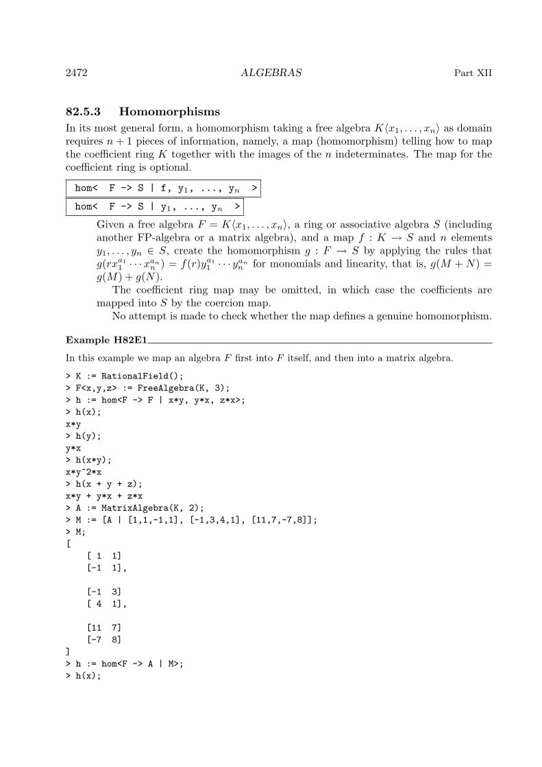
2472 ALGEBRAS Part XII
82.5.3 HomomorphismsIn its most general form, a homomorphism taking a free algebra K〈x1, . . . , xn〉 as domainrequires n+ 1 pieces of information, namely, a map (homomorphism) telling how to mapthe coefficient ring K together with the images of the n indeterminates. The map for thecoefficient ring is optional.
hom< F -> S | f, y1, ..., yn >
hom< F -> S | y1, ..., yn >
Given a free algebra F = K〈x1, . . . , xn〉, a ring or associative algebra S (includinganother FP-algebra or a matrix algebra), and a map f : K → S and n elementsy1, . . . , yn ∈ S, create the homomorphism g : F → S by applying the rules thatg(rxa1
1 · · ·xann ) = f(r)ya1
1 · · · yann for monomials and linearity, that is, g(M + N) =
g(M) + g(N).The coefficient ring map may be omitted, in which case the coefficients are
mapped into S by the coercion map.No attempt is made to check whether the map defines a genuine homomorphism.
Example H82E1
In this example we map an algebra F first into F itself, and then into a matrix algebra.
> K := RationalField();
> F<x,y,z> := FreeAlgebra(K, 3);
> h := hom<F -> F | x*y, y*x, z*x>;
> h(x);
x*y
> h(y);
y*x
> h(x*y);
x*y^2*x
> h(x + y + z);
x*y + y*x + z*x
> A := MatrixAlgebra(K, 2);
> M := [A | [1,1,-1,1], [-1,3,4,1], [11,7,-7,8]];
> M;
[
[ 1 1]
[-1 1],
[-1 3]
[ 4 1],
[11 7]
[-7 8]
]
> h := hom<F -> A | M>;
> h(x);

Ch. 82 FINITELY PRESENTED ALGEBRAS 2473
[ 1 1]
[-1 1]
> h(y);
[-1 3]
[ 4 1]
> h(x*y - y*z);
[ 35 -13]
[-32 -38]
82.6 Element Operations
82.6.1 Arithmetic OperatorsThe usual unary and binary ring operations are available for noncommutative polynomials,noting that multiplication is associative but noncommutative, of course.
+ a - a
a + b a - b a * b a ^ k a / b a div b
a +:= b a -:= b a *:= b a div:= b
82.6.2 Equality and Membership
a eq b a ne b
a in R a notin R
82.6.3 Predicates on Algebra Elements
IsZero(f) IsOne(f) IsMinusOne(f)
IsNilpotent(f) IsIdempotent(f)
IsUnit(f) IsZeroDivisor(f) IsRegular(f)
IsIrreducible(f) IsPrime(f)

2474 ALGEBRAS Part XII
82.6.4 Coefficients, Monomials, Terms and DegreeThe functions in this subsection allow one to access noncommutative polynomials.
Coefficients(f)
Given a noncommutative polynomial f with coefficients in R, this function returnsa sequence of ‘base’ coefficients, that is, a sequence of elements of R occurringas coefficients of the monomials in f . Note that the monomials are ordered, andthat the sequence of coefficients corresponds exactly to the sequence of monomialsreturned by Monomials(f).
LeadingCoefficient(f)
Given a noncommutative polynomial f with coefficients in R, this function returnsthe leading coefficient of f as an element of R; this is the coefficient of the leadingmonomial of f , that is, the first among the monomials occurring in f with respectto the ordering of monomials used in F .
TrailingCoefficient(f)
Given a noncommutative polynomial f with coefficients in R, this function returnsthe trailing coefficient of f as an element of R; this is the coefficient of the trailingmonomial of f , that is, the last among the monomials occurring in f with respectto the ordering of monomials used in F .
MonomialCoefficient(f, m)
Given a noncommutative polynomial f and a monomial m, this function returns thecoefficient with which m occurs in f as an element of R.
Monomials(f)
Given a noncommutative polynomial f ∈ F , this function returns a sequence ofthe monomials (monoid words) occurring in f . Note that the monomials in F areordered, and that the sequence of monomials corresponds exactly to the sequenceof coefficients returned by Coefficients(f).
LeadingMonomial(f)
Given a noncommutative polynomial f ∈ F this function returns the leading mono-mial of f , that is, the first monomial element of F that occurs in f , with respect tothe ordering of monomials used in F .
Terms(f)
Given a noncommutative polynomial f ∈ F , this function returns the sequence of(non-zero) terms of f as elements of F . The terms are ordered according to theordering on the monomials in F . Consequently the i-th element of this sequence ofterms will be equal to the product of the i-th element of the sequence of coefficientsand the i-th element of the sequence of monomials.

Ch. 82 FINITELY PRESENTED ALGEBRAS 2475
LeadingTerm(f)
Given a noncommutative polynomial f ∈ F , this function returns the leading termof f as an element of F ; this is the product of the leading monomial and the leadingcoefficient that is, the first among the monomial terms occurring in f with respectto the ordering of monomials used in F .
TrailingTerm(f)
Given a noncommutative polynomial f ∈ F , this function returns the trailing termof f as an element of F ; this is the last among the monomial terms occurring in fwith respect to the ordering of monomials used in F .
Length(m)
Given a noncommutative monomial (word) m, return the length of m, i.e., thenumber of letters of m. Note that this differs from the commutative case, where thenumber of terms in a polynomial is returned.
m[i]
Given a noncommutative monomial (word) m of length l, and an integer i with1 ≤ i ≤ l, return the i-th letter of m.
TotalDegree(f)
Given a noncommutative polynomial f , this function returns the total degree of f ,which is the maximum of the lengths of all monomials that occur in f . If f is thezero polynomial, the return value is −1.
LeadingTotalDegree(f)
Given a noncommutative polynomial, this function returns the leading total degreeof f , which is the length of the leading monomial of f .
Example H82E2
In this example we illustrate the above access functions.
> K := RationalField();
> F<x,y,z> := FreeAlgebra(K, 3);
> f := (3*x*y - 2*y*z)*(4*x - 7*z*y) + 23*x*y*z;
> f;
-21*x*y*z*y + 14*y*z^2*y + 12*x*y*x + 23*x*y*z - 8*y*z*x
> TotalDegree(f);
4
> Coefficients(f);
[ -21, 14, 12, 23, -8 ]
> Monomials(f);
[
x*y*z*y,
y*z^2*y,

2476 ALGEBRAS Part XII
x*y*x,
x*y*z,
y*z*x
]
> Terms(f);
[
-21*x*y*z*y,
14*y*z^2*y,
12*x*y*x,
23*x*y*z,
-8*y*z*x
]
> MonomialCoefficient(f, x*y*z);
23
> LeadingTerm(f);
-21*x*y*z*y
> LeadingCoefficient(f);
-21
> m := Monomials(f)[1];
> m;
x*y*z*y
> Length(m);
4
> m[1];
x
> m[2];
y
82.6.5 Evaluation
Evaluate(f, s)
Given an element f of a free algebra F = R〈x1, . . . , xn〉 and a sequence or tuples of ring or algebra elements of length n, return the value of f at s, that is, thevalue obtained by substituting xi = s[i]. This behaves in the same way as the homconstructor above.
If the elements of s lie in a ring and can be lifted into the coefficient ring R,then the result will be an element of R. If the elements of s cannot be lifted to thecoefficient ring, then an attempt is made to do a generic evaluation of f at s. Inthis case, the result will be of the same type as the elements of s.

Ch. 82 FINITELY PRESENTED ALGEBRAS 2477
Example H82E3
In this example we illustrate the above access functions.
> K := RationalField();
> F<x,y,z> := FreeAlgebra(K, 3);
> g := x*y + y*z;
> g;
x*y + y*z
> Evaluate(g, [1,2,3]);
8
> Parent($1);
Rational Field
> Evaluate(g, [y,x,z]);
x*z + y*x
> Parent($1);
Finitely presented algebra of rank 3 over Rational Field
Non-commutative Graded Lexicographical Order
Variables: x, y, z
82.7 Ideals and Grobner BasesMagma supports left-sided, right-sided, and two-sided ideals of free algebras. In general,there are not many operations applicable to single-sided ideals: quotients are supportedonly in the case of two-sided ideals.
Within the general context of fp-algebras, the term “basis” will refer to an orderedsequence of polynomials which generate an ideal. (Thus a basis may contain duplicatesand zero elements so it is dissimilar to a basis of a vector space.)
82.7.1 Creation of Ideals
ideal< A | L >
lideal< A | L >
rideal< A | L >
Given a free algebra A over a field K, return the two-sided (ideal), left-sided(lideal), or right-sided (rideal) of A generated by the elements of A specified bythe list L. Each term of the list L must be an expression defining an object of oneof the following types:(a)An element of A;(b)A set or sequence of elements of A;(c) An ideal of A;(d)A set or sequence of ideals of A.
Basis(I)

2478 ALGEBRAS Part XII
Given an ideal I, return the current basis of I. If a Grobner basis of I has beencomputed, that is returned.
BasisElement(I, i)
Given an ideal I together with an integer i, return the i-th element of the currentbasis of I. This the same as Basis(I)[i].
82.7.2 Grobner BasesGrobner bases (GBs) may be computed for any kind of ideal (left-, right-, or two-sided),but for single-sided ideals, the GBs are generally weak (i.e., they rarely differ much fromthe original generators of the ideals).
Unfortunately, the GB of a given ideal may not be finite. Thus the Buchberger or F4
algorithms below will run forever in such cases. One can interrupt any GB computationby pressing Ctrl-C. Alternatively, the function GroebnerBasis(S,d) below, which createsa truncated degree-d Grobner basis, can be used to set a limit on the degrees of the pairsconsidered, so the computation will always terminate.
As in the commutative case, when Magma constructs a GB G of an ideal I, then Gis always the unique sorted minimal reduced GB of I. Before this happens, an ideal willusually possess a basis which is not a Grobner basis, but that will be changed into theunique Grobner basis when the GB is computed. Thus the original basis will be discarded.See the procedure Groebner below for details on the algorithms available.
The unique Grobner basis will be computed automatically when necessary; theGroebner procedure below simply allows control of the algorithms used to compute theGrobner basis.
Groebner(I: parameters)
(Procedure.) Explicitly force a Grobner basis (GB) for I to be constructed. Thisprocedure is normally not necessary, as Magma will automatically compute the GBwhen needed, but it does allow one to control how the GB is constructed.
Faugere BoolElt Default : true
Magma has two algorithms for computing noncommutative GBs:(1)A noncommutative generalization (due to Allan Steel) of the Faugere F4
algorithm [Fau99], which works by specialized sparse linear algebra and isapplicable to two-sided ideals defined over a finite field or the rational field;
(2)The noncommutative Buchberger algorithm [CLO96, Chap. 2, §7] for idealsdefined over any field.
If the parameter Faugere is set to true, then the Faugere F4 algorithm will be used(if the field is a finite field or the rational field); otherwise the Buchberger algorithmis used.
The current implementation of the Faugere algorithm is usually very much fasterthan the Buchberger algorithm and usually does not take much more memory, sothat it is why it is selected by default. However, there may be examples for which it

Ch. 82 FINITELY PRESENTED ALGEBRAS 2479
may be more desirable to use the Buchberger algorithm (particularly to save somememory).
GroebnerBasis(I: parameters)
Given an ideal I, force the Grobner basis of I to be computed, and then return that.The parameters are the same as those for the procedure Groebner.
GroebnerBasis(S: parameters)
Given a set or sequence S of polynomials, return the unique Grobner basis of the two-sided ideal generated by S as a sorted sequence. This function is useful for computingGrobner bases without the need to construct ideals. The parameters are the sameas those for the procedure Groebner. See also the function GroebnerBasis(S,d)below, which creates a truncated degree-d Grobner basis.
GroebnerBasis(S, d: parameters)
Given a set or sequence S of polynomials, return the degree-d Grobner basis of theideal generated by S, which is the truncated Grobner basis obtained by ignoringS-polynomial pairs whose total degree is greater than d.
If the ideal is homogeneous, then it is guaranteed that the result is equal to theset of all polynomials in the full Grobner basis of the ideal whose total degree is lessthan or equal to d, and a polynomial whose total degree is less than or equal to dis in the ideal if and only if its normal form with respect to this truncated basis iszero. But if the ideal is not homogeneous, these last properties may not hold, butit may still be useful to construct the truncated basis.
The parameters are the same as those for the procedure Groebner.
82.7.3 VerbosityThis subsection describes the verbose flags available for the Grobner basis algorithms.There are separate verbose flags for each algorithm (Buchberger, etc.), but the all-encompassing verbose flag Groebner includes all these flags implicitly.
For each procedure provided for setting one of these flags, the value false is equivalentto level 0 (nothing), and true is equivalent to level 1 (minimal verbosity). For eachSet- procedure, there is also a corresponding Get- function to return the value of thecorresponding flag.
SetVerbose("Groebner", v)
(Procedure.) Change the verbose printing level for all Grobner basis algorithmsto be v. This includes all of the algorithms whose verbosity is controlled by flagssubsequently listed, as well as some other minor related algorithms. Currently thelegal levels are 0, 1, 2, 3, or 4. One would normally set this flag to 1 for minimalverbosity for Grobner basis-type computations, and possibly also set one or more ofthe following flags to levels higher than 1 for more verbosity.

2480 ALGEBRAS Part XII
SetVerbose("Buchberger", v)
(Procedure.) Change the verbose printing level for the Buchberger algorithm to bev. Currently the legal levels are 0, 1, 2, 3, or 4. If the value w of the Groebnerverbose flag is greater than v, then w is taken to be the current value of this flag.
SetVerbose("Faugere", v)
(Procedure.) Change the verbose printing level for the Faugere algorithm to be v.Currently the legal levels are 0, 1, 2, or 3. If the value w of the Groebner verboseflag is greater than v, then w is taken to be the current value of this flag.
82.7.4 Related FunctionsThe following functions and procedures perform operations related to Grobner bases.
MarkGroebner(I)
(Procedure.) Given an ideal I, mark the current basis of I to be the Grobner basisof the ideal with respect to the monomial order of the ideal. Note that the currentbasis must exactly equal the unique (reverse) sorted minimal reduced Grobner basisfor the ideal, as returned by the function GroebnerBasis. This procedure is usefulwhen one creates an ideal with a basis known to be the Grobner basis of the idealfrom a previous computation or for other reasons. If the basis is not the uniqueGrobner basis, the results are unpredictable.
Reduce(S)
Given a set or sequence S of polynomials, return the sequence consisting of thereduction of S. The reduction is obtained by reducing to normal form each elementof S with respect to the other elements and sorting the resulting non-zero elementsleft. Note that all Grobner bases returned by Magma are automatically reduced sothat this function would usually only be used just to simplify a set or sequence ofpolynomials which is not a Grobner basis.
Example H82E4
For a certain sequence B of noncommutative polynomials, we create the left-, right- and two-sidedideals generated by B. We note that for the first two cases, the GB is no different from B, butfor the two-sided case, the GB contains several more elements.
> K := RationalField();
> F<x,y,z> := FreeAlgebra(K, 3);
> B := [x^2 - y*z, x*y - y*z, y*x - z^2, y^3 - x*z];
> I := lideal<F | B>;
> I;
Left ideal of Finitely presented algebra of rank 3 over Rational Field
Non-commutative Graded Lexicographical Order
Variables: x, y, z
Basis:
[

Ch. 82 FINITELY PRESENTED ALGEBRAS 2481
x^2 - y*z,
x*y - y*z,
y*x - z^2,
y^3 - x*z
]
> GroebnerBasis(I);
[
y^3 - x*z,
x^2 - y*z,
x*y - y*z,
y*x - z^2
]
> I := rideal<F | B>;
> GroebnerBasis(I);
[
y^3 - x*z,
x^2 - y*z,
x*y - y*z,
y*x - z^2
]
> I := ideal<F | B>;
> Groebner(I);
> I;
Two-sided ideal of Finitely presented algebra of rank 3 over Rational Field
Non-commutative Graded Lexicographical Order
Variables: x, y, z
Groebner basis:
[
y*z^2*y - y*z^2,
y*z^3 - y*z^2,
z*y*z^2 - y*z^2,
z^2*y^2 - y*z^2,
z^2*y*z - y*z^2,
z^3*y - y*z^2,
z^4 - y*z^2,
x*z*x - y*z^2,
x*z*y - z^3,
x*z^2 - y*z^2,
y^3 - x*z,
y^2*z - z^2*y,
y*z*x - y*z^2,
y*z*y - y*z^2,
z^2*x - z^2*y,
x^2 - y*z,
x*y - y*z,
y*x - z^2
]
> NormalForm(x*y, I);

2482 ALGEBRAS Part XII
y*z
> NormalForm(y*x, I);
z^2
Finally, we compute some truncated bases of the two-sided ideal. For degree 2, the truncated GBhas no new polynomials while for degree 3, some are added. Only at degree 5 do we obtain thefull GB.
> GroebnerBasis(B, 2);
[
y^3 - x*z,
x^2 - y*z,
x*y - y*z,
y*x - z^2
]
> GroebnerBasis(B, 3);
[
x*z^2 - y*z^2,
y^3 - x*z,
y^2*z - z^2*y,
y*z*x - y*z^2,
y*z*y - y*z^2,
z^2*x - z^2*y,
x^2 - y*z,
x*y - y*z,
y*x - z^2
]
> #GroebnerBasis(I);
18
> #GroebnerBasis(B, 4);
16
> #GroebnerBasis(B, 5);
18
> GroebnerBasis(B, 5) eq GroebnerBasis(I);
true
82.8 Basic Operations on Ideals
In the following, note that the free algebra F itself is a valid ideal (the ideal containing 1).

Ch. 82 FINITELY PRESENTED ALGEBRAS 2483
82.8.1 Construction of New Ideals
I + J
Given ideals I and J belonging to the same algebra F , return the sum of I and J ,which is the ideal generated by the union of the generators of I and J .
I * J
Given ideals I and J belonging to the same algebra A, return the product of I andJ , which is the ideal generated by the products of the generators of I with those ofJ .
F / J
Given an algebra F over a field and an ideal J of F , return the fp-algebra F/J (seebelow).
Generic(I)
Given an ideal I of a generic algebra A, return A.
82.8.2 Ideal Predicates
I eq J
Given two ideals I and J belonging to the same algebra F , return whether I and Jare equal.
I ne J
Given two ideals I and J belonging to the same algebra F , return whether I and Jare not equal.
I notsubset J
Given two ideals I and J belonging to the same algebra F return whether I is notcontained in J .
I subset J
Given two ideals I and J belonging to the same algebra F return whether I iscontained in J .
IsZero(I)
Given an ideal I of the algebra F , return whether I is the zero ideal (contains zeroalone).

2484 ALGEBRAS Part XII
82.8.3 Operations on Elements of Ideals
f in I
Given a polynomial f from an algebra F , together with an ideal I of F , returnwhether f is in I.
NormalForm(f, I)
Given a polynomial f from an algebra F , together with an ideal I of F , return theunique normal form of f with respect to (the Grobner basis of) I. The normal formof f is zero if and only if f is in I.
NormalForm(f, S)
Given a polynomial f from an algebra F , together with a set or sequence S ofpolynomials from F , return a normal form of f with respect to S. This is notunique in general. If the normal form of f is zero then f is in the ideal generatedby S, but the converse is false in general. In fact, the normal form is unique if andonly if S forms a Groebner basis.
f notin I
Given a polynomial f from an algebra F , together with an ideal I of F , returnwhether f is not in I.
Example H82E5
We demonstrate the element operations with respect to an ideal of Q[x, y, z].
> F<x,y,z> := FreeAlgebra(RationalField(), 3);
> I := ideal<F | (x + y)^3, (y - z)^2, y^2*z + z>;
> NormalForm(y^2*z + z, I);
0
> NormalForm(x^3, I);
-x^2*y - x*y*x - x*y*z - x*z*y + x*z^2 - y*x^2 - y*x*y - y*z*x -
y*z*y - z*y*x - z*y*z + z^2*x + z^3
> NormalForm(z^4 + y^2, I);
z^4 + y*z + z*y - z^2
> x + y in I;
false

Ch. 82 FINITELY PRESENTED ALGEBRAS 2485
82.9 Changing Coefficient Ring
The ChangeRing function enables the changing of the coefficient ring of an algebra or ideal.
ChangeRing(I, S)
Given an ideal I of an algebra F = R[x1, . . . , xn] of rank n with coefficient ringR, together with a ring S, construct the ideal J of the algebra Q = S[x1, . . . , xn]obtained by coercing the coefficients of the elements of the basis of I into S. It isnecessary that all elements of the old coefficient ring R can be automatically coercedinto the new coefficient ring S. If R and S are fields and R is known to be a subfieldof S and the current basis of I is a Grobner basis, then the basis of J is markedautomatically to be a Grobner basis of J .
82.10 Finitely Presented Algebras
A finitely presented algebra (fp-algebra) in Magma is simply the quotient ring of a freealgebra F = R〈x1, . . . , xn〉 by an ideal J of F . It is an object of type AlgFP with elementsof type AlgFPElt.
The elements of fp-algebras are simply noncommutative polynomials which are alwayskept reduced to normal form modulo the ideal J of “relations”. Practically all operationswhich are applicable to noncommutative polynomials are also applicable in Magma toelements of fp-algebras (when meaningful).
If an fp-algebra A has finite dimension, considered as a vector space over its coefficientfield, then extra special operations are available for A and its elements.
82.11 Creation of FP-Algebras
One can create an fp-algebra simply by forming the quotient of a free algebra by an ideal(quo constructor or / function). A special constructor FPAlgebra is also provided toremove the need to create the free algebra.
NOTE: When one creates an fp-algebra, the ideal of relations is left unchanged, but assoon as one does just about any operation with elements of the algebra (such as printingor multiplying), then the Grobner basis of the underlying ideal will have to be computedto enable Magma to compute a unique form of each element of the algebra.
quo< F | J >
quo< F | a1, ..., ar >
Given a free algebra F and a two-sided ideal J of F , return the fp-algebra (quotientalgebra) F/J . The ideal J may either be specified as an ideal or by a list a1, a2,. . ., ar, of generators which all lie in F . The angle bracket notation can be used toassign names to the indeterminates: A<q, r> := quo< I | I.1 + I.2, I.2^2 -2, I.3^2 + I.4 >;.
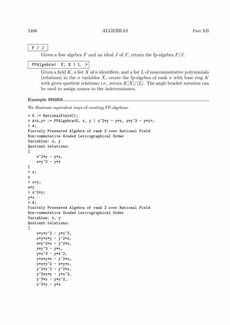
2486 ALGEBRAS Part XII
F / J
Given a free algebra F and an ideal J of F , return the fp-algebra F/J .
FPAlgebra< K, X | L >
Given a field K, a list X of n identifiers, and a list L of noncommutative polynomials(relations) in the n variables X, create the fp-algebra of rank n with base ring Kwith given quotient relations; i.e., return K[X]/〈L〉. The angle bracket notation canbe used to assign names to the indeterminates.
Example H82E6
We illustrate equivalent ways of creating FP-algebras.
> K := RationalField();
> A<x,y> := FPAlgebra<K, x, y | x^2*y - y*x, x*y^3 - y*x>;
> A;
Finitely Presented Algebra of rank 2 over Rational Field
Non-commutative Graded Lexicographical Order
Variables: x, y
Quotient relations:
[
x^2*y - y*x,
x*y^3 - y*x
]
> x;
x
> x*y;
x*y
> x^2*y;
y*x
> A;
Finitely Presented Algebra of rank 2 over Rational Field
Non-commutative Graded Lexicographical Order
Variables: x, y
Quotient relations:
[
x*y*x^2 - y*x^2,
x*y*x*y - y^2*x,
x*y^2*x - y^2*x,
x*y^3 - y*x,
y*x^3 - y*x^2,
y*x*y*x - y^2*x,
y*x*y^2 - x*y*x,
y^2*x^2 - y^2*x,
y^2*x*y - y*x^2,
y^3*x - y*x^2,
x^2*y - y*x

Ch. 82 FINITELY PRESENTED ALGEBRAS 2487
]
The following is equivalent.
> K := RationalField();
> F<x,y> := FreeAlgebra(K, 2);
> A<x,y> := quo<F | x^2*y - y*x, x*y^3 - y*x>;
82.12 Operations on FP-Algebras
This section describes operations on fp-algebras. Most of the operations are very similarto those for noncommutative free algebras; such operations are done by mapping thecomputation to the preimage ideal and then by mapping the result back into the fp-algebra.See the corresponding functions for the noncommutative free algebras for details.
A . i
Given an fp-algebra A, return the i-th indeterminate of A as an element of A.
CoefficientRing(A)
Return the coefficient ring of the fp-algebra A.
Rank(A)
Return the rank of the fp-algebra A (the number of indeterminates of A).
DivisorIdeal(I)
Given an ideal I of an fp-algebra A which is the quotient ring F/J , where F is afree algebra and J an ideal of F , return the ideal J .
PreimageIdeal(I)
Given an ideal I of an fp-algebra A which is the quotient ring F/J , where F is afree algebra and J an ideal of F , return the ideal I ′ of F such that the image of I ′
under the natural epimorphism F → A is I.
PreimageRing(A)
Given an fp-algebra A which is the quotient ring F/J , where F is a free algebra andJ an ideal of F , return the free algebra F .
OriginalRing(A)
Return the generic free algebra F such that A is F/J for some ideal J of F .
IsCommutative(A)
Return whether the algebra A is commutative.

2488 ALGEBRAS Part XII
I eq J
Given two ideals I and J of the same fp-algebra A, return true if and only if I andJ are equal.
I subset J
Given two ideals I and J of the same fp-algebra A, return true if and only if I iscontained in J .
I + J
Given two ideals I and J of the same fp-algebra A, return the sum I + J .
I * J
Given two ideals I and J of the same fp-algebra A, return the product I ∗ J .
IsProper(I)
Given an ideal I of the fp-algebra A, return whether I is proper; that is, whether Iis strictly contained in A.
IsZero(I)
Given an ideal I of the fp-algebra A, return whether I is the zero ideal. Note thatthis is equivalent to whether the preimage ideal of I is the divisor ideal of A.
82.13 Finite Dimensional FP-Algebras
If an fp-algebra A has finite dimension, considered as a vector space over its coefficientfield, then extra special operations are available for A and the elements of A.
Dimension(A)
Given a finite dimensional fp-algebra A, return the dimension of A.
VectorSpace(A)
Given a finite dimensional fp-algebra A, construct the vector space V isomorphic toA, and return V together with the isomorphism f from A onto V .
MatrixAlgebra(A)
Given a finite dimensional fp-algebra A, construct the matrix algebra M isomorphicto A, and return M together with the isomorphism f from A onto M .
Algebra(A)
Given a finite dimensional fp-algebra A, construct the associative structure-constantalgebra S isomorphic to A, and return S together with the isomorphism f from Aonto S.

Ch. 82 FINITELY PRESENTED ALGEBRAS 2489
RepresentationMatrix(f)
Given an element f of a finite dimensional fp-algebra A, return the representationmatrix of f , which is a d by d matrix over the coefficient field of A which representsf (where d is the dimension of A).
IsUnit(f)
Given an element f of a finite dimensional fp-algebra A defined over a field, returnwhether f is a unit.
IsNilpotent(f)
Given an element f of a finite dimensional fp-algebra A defined over a field, returnwhether f is nilpotent, and if so, return also the smallest q such that fq = 0.
MinimalPolynomial(f)
Given an element f of a finite dimensional fp-algebra A defined over a field, returnthe minimal polynomial of f as a univariate polynomial over the coefficient field ofA.
Example H82E7
We demonstrate the functions available for finite-dimensional fp-algebras.
> K := RationalField();
> A<x,y,z> := FPAlgebra<K, x,y,z |
> x^2 - y*z*y + z, y^2 - y*x*y + 1, z^2 - y*x*y - x*z*x>;
> A;
Finitely Presented Algebra of rank 3 over Rational Field
Non-commutative Graded Lexicographical Order
Variables: x, y, z
Quotient relations:
[
y^4 - 7/2*z^2*x + z^3 - 1/2*x^2 + 2*y^2 + z*x + z^2 + x + 1,
z*y*x^2 + y^3 - z^2*y + y,
z^2*y*x - 1/2*z*y*z - z^2*y - 1/2*y*x,
z^2*y*z - 3/2*y*x^2 - 3/4*z*y*z - 3/2*z^2*y - 3/4*y*x - y*z - z*y,
z^3*x - 3/2*z^3 - 1/2*z*x,
z^3*y - 3/2*y*x^2 - 3/4*z*y*z - 3/2*z^2*y - 3/4*y*x - y*z - z*y,
z^4 - 2*z^2*x - 9/4*z^3 + 3/2*y^2 - 3/4*z*x - 1/2*z^2 + x + 3/2,
x^3 + 3/2*z^2*x - z^3 + 1/2*x^2 + z*x,
y^2*x - y^2 - 1,
y^2*z + 3/2*z^2*x - z^3 + 1/2*x^2 + z,
y*z*x - z*y*x,
y*z*y - x^2 - z,
y*z^2 - z^2*y,
z*x^2 + y^2 - z^2 + 1,
z*y^2 + 3/2*z^2*x - z^3 + 1/2*x^2 + z,
x*y - y*x,

2490 ALGEBRAS Part XII
x*z - z*x
]
> IsCommutative(A);
false
> y*z;
y*z
> z*y;
z*y
> U<u> := PolynomialRing(K);
> MinimalPolynomial(x);
u^8 - 7/2*u^7 + 4*u^6 - 3/2*u^5 - 1/2*u^4 + 2*u^3 - 2*u^2
> MinimalPolynomial(y);
u^16 - u^12 + 3*u^10 + u^8 - 10*u^6 - 15*u^4 - 9*u^2 - 2
> Dimension(A);
18
> V, Vf := VectorSpace(A);
> V;
Full Vector space of degree 18 over Rational Field
> Vf(x);
(0 0 0 1 0 0 0 0 0 0 0 0 0 0 0 0 0 0)
> [V.i@@Vf: i in [1 .. Dimension(V)]];
[
1,
z,
y,
x,
z^2,
z*y,
z*x,
y*z,
y^2,
y*x,
x^2,
z^3,
z^2*y,
z^2*x,
z*y*z,
z*y*x,
y^3,
y*x^2
]
> M, Mf := MatrixAlgebra(A);
> M;
Matrix Algebra of degree 18 with 4 generators over Rational Field
> M.1;
[0 0 0 1 0 0 0 0 0 0 0 0 0 0 0 0 0 0]
[0 0 0 0 0 0 1 0 0 0 0 0 0 0 0 0 0 0]
[0 0 0 0 0 0 0 0 0 1 0 0 0 0 0 0 0 0]
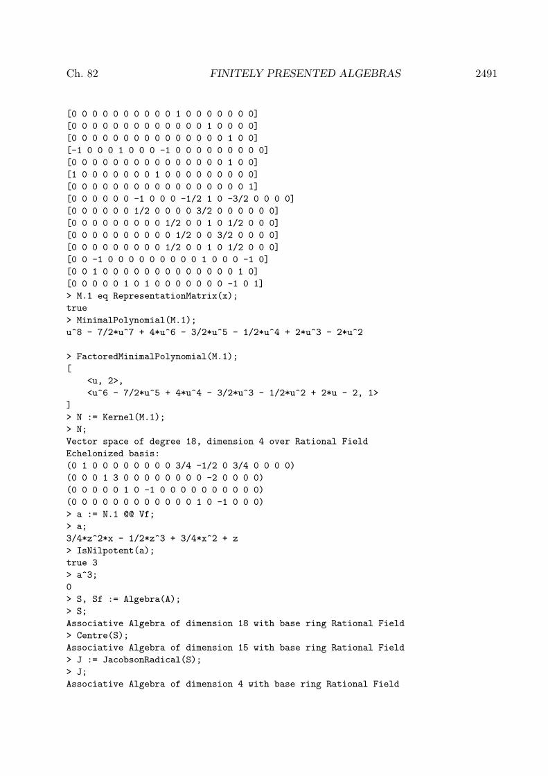
Ch. 82 FINITELY PRESENTED ALGEBRAS 2491
[0 0 0 0 0 0 0 0 0 0 1 0 0 0 0 0 0 0]
[0 0 0 0 0 0 0 0 0 0 0 0 0 1 0 0 0 0]
[0 0 0 0 0 0 0 0 0 0 0 0 0 0 0 1 0 0]
[-1 0 0 0 1 0 0 0 -1 0 0 0 0 0 0 0 0 0]
[0 0 0 0 0 0 0 0 0 0 0 0 0 0 0 1 0 0]
[1 0 0 0 0 0 0 0 1 0 0 0 0 0 0 0 0 0]
[0 0 0 0 0 0 0 0 0 0 0 0 0 0 0 0 0 1]
[0 0 0 0 0 0 -1 0 0 0 -1/2 1 0 -3/2 0 0 0 0]
[0 0 0 0 0 0 1/2 0 0 0 0 3/2 0 0 0 0 0 0]
[0 0 0 0 0 0 0 0 0 1/2 0 0 1 0 1/2 0 0 0]
[0 0 0 0 0 0 0 0 0 0 1/2 0 0 3/2 0 0 0 0]
[0 0 0 0 0 0 0 0 0 1/2 0 0 1 0 1/2 0 0 0]
[0 0 -1 0 0 0 0 0 0 0 0 0 1 0 0 0 -1 0]
[0 0 1 0 0 0 0 0 0 0 0 0 0 0 0 0 1 0]
[0 0 0 0 0 1 0 1 0 0 0 0 0 0 0 -1 0 1]
> M.1 eq RepresentationMatrix(x);
true
> MinimalPolynomial(M.1);
u^8 - 7/2*u^7 + 4*u^6 - 3/2*u^5 - 1/2*u^4 + 2*u^3 - 2*u^2
> FactoredMinimalPolynomial(M.1);
[
<u, 2>,
<u^6 - 7/2*u^5 + 4*u^4 - 3/2*u^3 - 1/2*u^2 + 2*u - 2, 1>
]
> N := Kernel(M.1);
> N;
Vector space of degree 18, dimension 4 over Rational Field
Echelonized basis:
(0 1 0 0 0 0 0 0 0 0 3/4 -1/2 0 3/4 0 0 0 0)
(0 0 0 1 3 0 0 0 0 0 0 0 0 -2 0 0 0 0)
(0 0 0 0 0 1 0 -1 0 0 0 0 0 0 0 0 0 0)
(0 0 0 0 0 0 0 0 0 0 0 0 1 0 -1 0 0 0)
> a := N.1 @@ Vf;
> a;
3/4*z^2*x - 1/2*z^3 + 3/4*x^2 + z
> IsNilpotent(a);
true 3
> a^3;
0
> S, Sf := Algebra(A);
> S;
Associative Algebra of dimension 18 with base ring Rational Field
> Centre(S);
Associative Algebra of dimension 15 with base ring Rational Field
> J := JacobsonRadical(S);
> J;
Associative Algebra of dimension 4 with base ring Rational Field

2492 ALGEBRAS Part XII
> L := [J.i@@Sf: i in [1 .. 4]];
> L;
[
3/4*z^2*x - 1/2*z^3 + 3/4*x^2 + z,
-2*z^2*x + 3*z^2 + x,
-y*z + z*y,
-z*y*z + z^2*y
]
> [MinimalPolynomial(x): x in L];
[
u^3,
u^2,
u^3,
u^2
]
82.14 Vector Enumeration
Vector enumeration (originally misnamed module enumeration) is an algorithm for con-verting a finitely-presented module for a finitely-presented algebra into a concrete vectorspace on which the algebra has explicit matrix action. The algebra may be the group al-gebra of an fp-group, in which case the resulting module will be a matrix representation ofthe group, or it might be a more general fp-algebra, such as a Hecke algebra or a quotientof a polynomial ring.
82.14.1 Finitely Presented ModulesFor a ring R, let M be an R-module M , generated as an R-module by s elementsm1, . . . ,ms. There is an R-module epimorphism ψ : Rs 7→M , given by
(r1, . . . , rs) 7→ m1r1 + · · ·+msrs.
This shows that M is isomorphic to As/ kerψ.If kerψ is generated as an R-module by a finite set L then we will say that M is
presented by s generators and the relators L.
82.14.2 S-algebrasSuppose there is another ring S, equipped with a ring homomorphism φ : S 7→ R, suchthat φ(S) is central in R. In this situation any R-module can be described as an S-module,on which R acts as a ring of S-module endomorphisms. We say that R is an S-algebra. Inparticular, when S is a field k, any R-module is a k-vector space. If such a module V hasfinite k-dimension n, then V is characterised by this dimension and R will act on it as asubring of Mn(k).

Ch. 82 FINITELY PRESENTED ALGEBRAS 2493
82.14.3 Finitely Presented AlgebrasGiven a finite set X, and a ring S, we can define the free S-algebra A generated by X.This can be seen either as the monoid algebra of the free monoid of words in X, or as allexpressions in X and k, combined by addition and multiplication.
Given a finite set R ⊂ A we can define
P =A
〈ARA〉 .
We say that P is a finitely-presented S-algebra, with generators X and relators R, andwrite it
P = 〈X | R〉 .The monoid algebra of any finitely-presented monoid (or group, of course) is finitely-
presented, since
k 〈X | l1 = r1, . . . , lk = rk〉monoid = 〈X | l1 − r1, . . . , lk − rk〉k−algebra .
Furthermore, any quotient of a finitely-presented algebra by a finitely-generated two-sidedideal is finitely-presented. This gives us the general form of a finitely-presented algebra inMagma, as the quotient of the monoid algebra of an fp-monoid, by the two-sided idealgenerated by some additional relators.
82.14.4 Vector EnumerationThe vector enumeration algorithm explicitly reconciles these two descriptions of an R-module, in the case where R is a finitely presented k-algebra for a field k, and M is afinitely presented R-module, which also has finite k-dimension.
Given the presentation of R as k-algebra, and that of M as R-module, it computes thek-dimension of M and the matrices giving the action of the generators of R on M . If Mhas infinite k-dimension the algorithm will fail to terminate.
Example H82E8
We consider some examples in the abstract. Below we will see how these and other calculationsmay be performed in Magma.(1) A permutation moduleIn practice, it is always better to use the classical Todd-Coxeter algorithm to construct permuta-tion representations of groups.We know that the group with presentation
⟨a, b | a4 = b2 = (ab)2 = 1
⟩
is the dihedral group of order 8. Its group algebra over any field k is thus the fp-k-algebra
⟨a, b, a′, b′ | aa′ − 1, a′a− 1, bb′ − 1, b′b− 1, a4 − 1, b2 − 1, (ab)2 − 1
⟩.

2494 ALGEBRAS Part XII
The permutation module of degree 4 of this algebra is presented by one generator (as it is transi-tive) and the submodule generator b− 1.Applying the algorithm to this case we obtain the matrices
a =
0 0 1 01 0 0 00 0 0 10 1 0 0
b =
1 0 0 00 0 1 00 1 0 00 0 0 1
and their inverses for a′ and b′.(2) A quotient of a permutation moduleLike all permutation modules, this one fixes the all-ones vector (1, 1, 1, 1), which we can see to bean image of 1 + a′(1 + b + a′). We can construct the quotient of the permutation module by this1-dimensional submodule by adding that word to the submodule generators. This gives
a =
(0 0 11 0 0−1 −1 −1
)b =
(1 0 00 0 10 1 0
).
(3) A non-cyclic moduleA permutation module of a group-ring is cyclic (that is, generated as a module by one element) justwhen the permutation representation is transitive. An intransitive permutation representation canbe easily constructed from its transitive components, but in general it is not so easy to constructan arbitrary module from cyclic submodules. Accordingly it can be worthwhile to constructnon-cyclic modules directly.As an example we take two copies of the representation constructed in example one, and fuse theirone-dimensional submodules. The generators and relators are as before, and now s = 2 and thesubmodule generators are a2 = (b− 1, 0), (0, b− 1), (1 + a′(1 + a′ + b),−1− a′(1 + a′ + b)). Weobtain a representation of degree seven, given by
a =
0 0 0 1 0 0 00 0 0 0 0 0 11 0 0 0 0 0 00 0 0 0 1 0 00 0 1 0 0 0 00 1 0 0 0 0 01 −1 1 1 1 −1 −1
b =
1 0 0 0 0 0 00 1 0 0 0 0 00 0 0 1 0 0 00 0 1 0 0 0 00 0 0 0 1 0 00 0 0 0 0 0 10 0 0 0 0 1 0
.
82.14.5 The IsomorphismIn determining the k-dimension of M , and giving matrices representing the action of Ron M , the algorithm is, in effect, constructing a k-vector space, on which R has matrixaction, and which is R-module isomorphic to M , which is formally a quotient module ofRs. The algorithm also computes this isomorphism, giving images in the vector space forthe s standard generators of Rs and pre-images in Rs of the basis of the vector space.
In example (1) above, we find that the module generator has image (1, 0, 0, 0), whilethe basis vectors have pre-images 1, a′, a′2 and b.
In example (3) the images of the two module generators are (1, 0, 0, 0, 0, 0, 0) and(0, 1, 0, 0, 0, 0, 0) while the basis vectors are images of (1, 0), (0, 1), (a′, 0) ,(a, 0), (a2, 0),(0, a′) and (0, a).

Ch. 82 FINITELY PRESENTED ALGEBRAS 2495
82.14.6 Sketch of the AlgorithmThe algorithm is based on the Haselgrove-Leech-Trotter (HLT) version of the Todd-Coxeteralgorithm, which we consider as a means of constructing the permutation representationof a finitely-presented group on the cosets of a finitely generated subgroup.
The algorithm proceeds by manipulating a partial action of the free algebra on a vectorspace. This is represented as a table, with columns indexed by the generators of thealgebra, and rows indexed by the basis of the space. Each entry is either a vector or ⊥,signifying that no action is given.
We can extend this to a “complete action with side-effects”, by adding a new row tothe table whenever needed. We call this the action with defining.
The action of the fp-algebra P on M gives an action for the free algebra A, and ourobjective is to modify out partial action until it becomes this action. We know certainthings about this action, which drive our modification process:1. It is a complete action.2. The relators of P annihilate every vector.3. The images in the space of the relators of M are zero.4. The space contains images of the R-module generators of M .The algorithm begins by applying the fourth fact and creating s linearly independentvectors. It then applies the third, computing the action with defining of the relators ofM (the set called L above). The fact that these images should be zero gives a lineardependence among our basis vectors (called a coincidence), which we use to reduce theirnumber. As we do this, we have to take care not to lose the information already in thetable, which may give rise to further coincidences.
We now start to exploit the second fact aboutM , constructing the action (with defining)of the relators of P , on the basis vectors, and applying the resulting coincidences. Thisprocess may not terminate, as we are defining new basis vectors on the one hand, andremoving them through coincidences on the other. It is possible to prove, however, that ifM is in fact finite-dimensional then the process will terminate.
The first fact is applied by adding the relators x− x for each x ∈ X to the relators ofP , so that the image of every basis vector under each x is sure to be defined.
82.14.7 WeightsThe above sketch leaves open the question of the order in which the relators are appliedto the basis vectors. The proof that the algorithm completes when M is finite-dimensionalimposes some rather loose constraints, but within these constraints there is considerablechoice.
The implementation in Magma uses a system of weights. Each relator r is assigneda weight wr by the user, and each basis vector e has a weight we. There is a currentweight w, which increases as the computation progresses, and at weight w all basis vector,relator pairs (b, r) such that wb + wr ≤ w, which have not been processed already, areprocessed. New basis vectors defined during this process are assigned weight w. Theinitial basis vectors and those defined during processing of the submodule generators areassigned weight 1. See below for details of how to set the weights, and their default values.
2496 ALGEBRAS Part XII
82.14.8 Setup FunctionsFor V2.11, the following functions create the old representation for fp-algebras which arenecessary for the Vector Enumeration algorithm. These are compatible with older versionsof Magma. See the examples below for examples of how to use these functions.
FreeAlgebra(R, M)
FreeAlgebra(R, G)
Construct the special fp-algebra over the ring R and the monoid M or the group G,for use in the Vector Enumeration algorithm.
82.14.9 The Quotient Module Function
QuotientModule(A, S)
Given an fp-k-algebra A, for a field k, with r generators, and a submodule N of thefree A-module of rank s specified by S, construct an A-module isomorphic to thequotient module As/N together with the isomorphism.
The three values returned are:M a sequence of r n× n matrices with entries in k;I a sequence of s vectors of length n with entries in k;P a sequence of n elements of the free A-module As.
The matrices M specify a homomorphism from A to Endk(kn), under whichkn becomes an A-module isomorphic to As/N . That isomorphism is given in onedirection by the vectors I, which are the images in kn of the s generators (1, 0, . . . , 0),(0, 1, 0, . . . , 0), . . . , (0, . . . , 0, 1) of As. In the other direction, the elements P giverepresentatives for the images in As/N of the images of the n standard basis elementsof kn.
The submodule N may be specified by the parameter S in three ways:(1)S may simply be N , a finitely generated submodule of a free A-module (except
that such an object cannot currently be created).(2)S may be a finitely generated right ideal of A, in which case s = 1 and N is S
considered as a submodule of A considered as a right module for itself.(3)S may be a sequence of elements of a free A-module As, in which case N is the
submodule that they generate (this is a stand in for 1 and could be removedwhen 1 is implemented).
82.14.10 Structuring PresentationsThe relations used by the vector enumeration algorithm come from three sources:(1)The relations of the fp-group or fp-monoid underlying A.(2)The relations of A itself.(3)The generators of N .

Ch. 82 FINITELY PRESENTED ALGEBRAS 2497
The third group play the same role as subgroup generators in the Todd-Coxeter algorithm,and are treated specially, while the first two groups are logically equivalent, forming therelations of A in the variety of free finitely-generated associative algebras. However, whenthe underlying monoid of A is actually an fp-group G, the vector enumeration algorithmcan use a more efficient technique to process the relations of G, and can take advantage ofthe fact that the generators of G are known to be invertible.
This greatly improves the performance of the algorithm, and so users are recommendedto ensure as far as possible that:(1) If the underlying monoid of an fp-algebra is in fact an fp-group then it should be
presented to Magma as such.(2)Relations which can be written as equations between monomials should be given as
relations of the underlying monoid, rather than as relations of the algebra.
82.14.11 Options and ControlsThe QuotientModule function supports a large selection of optional arguments.
82.14.12 WeightsThe processing of the relations of A by the vector enumeration algorithm depends onweights which are assigned to those relations (see above). The higher the weight of arelation the later it will be processed. By default, all relations are given weight 3, exceptthose arising from relators of an fp-group, which are given weight equal to half the lengthof the relator.
Separate weights are used in lookahead mode, with the same default values.
QuotientModule(A, S)
MonomialWeights [ RngIntElt ] Default :
MonWts [ RngIntElt ] Default :
This option sets the sequence of weights for the relations derived from the rela-tions of the underlying monoid of A. The weights w1, w2, etc. are applied to therelations in the order in which they appear. If there are fewer weights than relationsthe remaining relations are assigned the default weight; if there are more weightsthan relations the extra weights are silently discarded.
Unless the MonomialLookaheadweights or MonLWts parameters are present,these weights are also used in lookahead mode.
MonomialLookaheadWeights
[ RngIntElt ] Default :
MonLWts [ RngIntElt ] Default :
This option sets the sequence of weights for the relations derived from the relationsof the underlying monoid of A in lookahead mode only. It is otherwise similar toMonomialWeights.
AlgebraWeights [ RngIntElt ] Default :

2498 ALGEBRAS Part XII
AlgWts [ RngIntElt ] Default :
This option sets the sequence of weights for the relations given explicitly as relationsof the algebra A. It is otherwise similar to MonomialWeights.
AlgebraLookaheadWeights
[ RngIntElt ] Default :
AlgLWts [ RngIntElt ] Default :
This option sets the sequence of weights for the relations given explicitly as relationsof the algebra A in lookahead mode only. It is otherwise similar to AlgebraWeights.
82.14.13 Limits
QuotientModule(A, S)
Options in this group set limits on the progress of the algorithm. If the calculationcannot be performed under these constraints the value undef is returned, unless theErrorOnFail option was set, in which case a run-time error is generated.
MaximumDimension RngIntElt Default : ∞MaxDim [ RngIntElt ] Default : ∞This sets a limit of n on the dimension of the vector-space constructed, and on
the dimension of the intermediate spaces used in the construction.By default there is no limit, except for available memory.
MaximumTime FldReElt Default : ∞MaxTime FldReElt Default : ∞
This sets a limit on the CPU time available for the vector enumeration. The limitis given as a real number t and is measured in seconds.
This limit is only checked at certain points in the calculation, so it is possiblefor a vector enumeration to over-run, possibly by a significant amount.
By default, there is no limit.
MaximumWeight RngIntElt Default : 100
MaxWt RngIntElt Default : 100
This sets a limit on the maximum weight of (basis vector, relation) pairs that willbe used by the algorithm.
The weight of a basis vector is the weight of the pair that was being processedwhen it was defined. The weight of a pair is the weight of the basis vector plus theweight of the relation (see above).
The default limit is 100.

Ch. 82 FINITELY PRESENTED ALGEBRAS 2499
82.14.14 Logging
QuotientModule(A, S)
There are a number of options to control the level of detail provided in the informa-tional message from the vector enumerator. When multiple contradictory optionsare given the first one given takes precedence.
NoLogging BoolElt Default : false
NoLog BoolElt Default : false
Silent BoolElt Default : false
This option turns off all the informational messages produced by the vectorenumerator.
MaximumLogging BoolElt Default : false
MaxLog BoolElt Default : false
This option turns on the highest possible level of detail in the informational mes-sages. This is too detailed for almost all purposes except debugging.
LogActions RngIntElt Default : 0LogAct RngIntElt Default : 0
This option sets the level of messages about the computation of the action of thealgebra on the vector space under construction. At level 0 (the default) no messagesare produced. All other levels produce copious output, with all levels above 2 beingequivalent.
LogCoincidences RngIntElt Default : 0LogCoin RngIntElt Default : 0
This option sets the level of messages about the coincidences discovered and theprocessing of them. At level 0 (the default) no messages are produced. At level 1every coincidence and deduction is recorded when it is discovered and when it isprocessed. At level 2 or higher the operation of finding the undeleted image of avector is also recorded.
LogInitialization RngIntElt Default : 0LogInitialisation RngIntElt Default : 0LogInit RngIntElt Default : 0
This option sets the level of messages about the initialisation of new basis vectors.At level 0 (the default) no messages are produced. All other levels produce a messagewhenever a new basis vector is defined.
LogPacking RngIntElt Default : 1LogPack RngIntElt Default : 1
This option sets the level of messages about the reclamation of free space in thetables used by the algorithm. At level 0 no messages are produced. At level 1 (the

2500 ALGEBRAS Part XII
default) it produces a message each time the pack routine is called. At level 2 orhigher it records the exact renaming used to reclaim the space.
LogPushes RngIntElt Default : 0LogPush RngIntElt Default : 0
This option sets the level of messages about the pushing (or tracing) of (basis vector,relation) pairs. At level 0 (the default) it produces no messages. At level 1 a messageis produced for each push that is started. At level 2 or higher the outcome of thepush is also recorded.
LogProgress RngIntElt Default : 0LogStages RngIntElt Default : 0
This option sets the level of messages about the overall progress of the algorithm.At level 0 no messages are produced. At level 1, simple messages are printed as thealgorithm passes through its major stages. At level 2 the relations are printed asthey are read in, and the complete action on the final module is printed. At level 3or higher the action is also printed after the processing of submodule generators iscomplete.
LogWeightChanges RngIntElt Default : 1LogWt RngIntElt Default : 1
This option sets the level of messages about changes in the current weight (ie theweight of (basis vector, relation pairs) currently being pushed. At level 0 no suchmessages are produced. At level 1 (the default) or higher a message giving the newweight and the current dimension is printed.
82.14.15 Miscellaneous
QuotientModule(A, S)
Lookahead BoolElt Default : true
This option controls whether, and to what extent, lookahead is used. If x isfalse then lookahead is not used. If x is true, the default, the lookahead by thedefault amount (two weights) is used. If x is a positive integer n then lookahead nweights is used. A sufficiently large value of n is equivalent to complete lookahead.Lookahead is commenced approximately every time the dimension doubles.
EarlyClosing BoolElt Default : false
Early BoolElt Default : false
This option permits the algorithm to stop as soon as the table represents a completeaction (but see below), without checking to see whether the action satisfies all therelations. In practice this action is usually correct. The default behaviour is tocontinue and check all the relations.
EarlyClosingMinimum RngIntElt Default :
ECMin RngIntElt Default :

Ch. 82 FINITELY PRESENTED ALGEBRAS 2501
This option sets a minimum dimension at which the algorithm may stop withoutchecking all the relators. It implies EarlyClosing.
EarlyClosingMaximum RngIntElt Default :
ECMax RngIntElt Default :
This option sets a maximum dimension at which the algorithm aamy stop withoutchecking all the relators. It implies EarlyClosing.
ConstructMorphism BoolElt Default : true
Morphism BoolElt Default : true
This option controls whether the third return value of the QuotientModule functionis in fact computed. A small overhead of time and space is required to compute it,and many applications do not need it, so this option is provided. When b is true(the default) the third return value is computed, when b is false it is not.
ErrorOnFail BoolElt Default :
ErrFail BoolElt Default :
This option controls the behaviour of the program if there is insufficient time orspace to complete the calculation, or if the calculation has not been completedwhen the maximum weight is reached. If it is present a run-time error is generated,otherwise the value undef is returned.
Example H82E9
First we repeat the examples above, in Magma. The permutation action of D8
> d8<a,b> := Group<a,b | a^4 = b^2 = (a*b)^2 = 1>;
> q := RationalField();
> a1<a,b> := FreeAlgebra(q,d8);
> i1 := rideal<a1 | b-1 >;
> mats, im, preim := QuotientModule(a1,i1);
Read Input
Done submodule generators
Starting weight 2 in define mode, 1 alive out of 2
Starting weight 3 in define mode, 1 alive out of 2
Looking ahead ...
Starting weight 4 in lookahead mode, 4 alive out of 5
Starting weight 5 in lookahead mode, 4 alive out of 5
...done
Packing 5 to 4
Starting weight 4 in define mode, 4 alive out of 4
Starting weight 5 in define mode, 4 alive out of 4
Starting weight 6 in define mode, 4 alive out of 4
Starting weight 7 in define mode, 5 alive out of 6
Starting weight 8 in define mode, 6 alive out of 7
Starting weight 9 in define mode, 4 alive out of 7
Starting weight 10 in define mode, 4 alive out of 7
Closed, 7 rows defined

2502 ALGEBRAS Part XII
Packing 7 to 4
4 live dimensions
Successful
> mats;
[
[0 0 1 0]
[1 0 0 0]
[0 0 0 1]
[0 1 0 0],
[1 0 0 0]
[0 0 1 0]
[0 1 0 0]
[0 0 0 1]
]
> im;
[
(1 0 0 0)
]
> preim;
[ Id(), a^-1, a^-1 * b, a^-2 ]
>
Example H82E10
A quotient of that module.We continue from the last example and set:
> d8<a,b> := Group<a,b | a^4 = b^2 = (a*b)^2 = 1>;
> q := RationalField();
> a1<a,b> := FreeAlgebra(q,d8);
> i2 := rideal<a1 | b-1, 1+a^3+a^3*b+a^2>;
> mats, im, preim := QuotientModule(a1,i2);
Read Input
Done submodule generators
Starting weight 2 in define mode, 4 alive out of 6
Starting weight 3 in define mode, 5 alive out of 7
Starting weight 4 in define mode, 3 alive out of 7
Starting weight 5 in define mode, 3 alive out of 7
Closed, 7 rows defined
Packing 7 to 3
3 live dimensions
Successful
> mats;
[
[ 0 1 0]
[ 0 0 1]
[-1 -1 -1],

Ch. 82 FINITELY PRESENTED ALGEBRAS 2503
[ 1 0 0]
[-1 -1 -1]
[ 0 0 1]
]
82.15 Bibliography[CLO96] David Cox, John Little, and Donal O’Shea. Ideals, Varieties and Algorithms.
Undergraduate Texts in Mathematics. Springer, New York–Berlin–Heidelberg, 2ndedition, 1996.
[Fau99] Jean-Charles Faugere. A new efficient algorithm for computing Grobner bases(F4). Journal of Pure and Applied Algebra, 139 (1-3):61–88, 1999.
[Li02] Huishi Li. Noncommutative Grobner Bases and Filtered-Graded Transfer, vol-ume 1795 of Lecture Notes in Math. Springer-Verlag, Berlin–Heidelberg–New York,2002.
[Mor94] Teo Mora. An introduction to commutative and noncommutative Grobnerbases. Theoretical Computer Science, 134:134–173, 1994.


83 MATRIX ALGEBRAS83.1 Introduction . . . . . . . . 2509
83.2 Construction of Matrix Algebrasand their Elements . . . . . 2509
83.2.1 Construction of the Complete MatrixAlgebra . . . . . . . . . . . . 2509
MatrixAlgebra(S, n) 2509MatrixRing(S, n) 2509
83.2.2 Construction of a Matrix . . . . . 2509
elt< > 2509! 2509CambridgeMatrix(t, K, n, Q) 2510CompanionMatrix(p) 2510DiagonalMatrix(R, Q) 2510MatrixUnit(R, i, j) 2510Random(R) 2510ScalarMatrix(R, t) 2510! 2510! 2510! 251083.2.3 Constructing a General Matrix Alge-
bra . . . . . . . . . . . . . . 2511
MatrixAlgebra< > 2511MatrixRing< > 2511
83.2.4 The Invariants of a Matrix Algebra 2512
. 2512BaseRing(R) 2512CoefficientRing(R) 2512Degree(R) 2512Generators(R) 2512Generic(R) 2512BaseModule(R) 2512NumberOfGenerators(R) 2512Ngens(R) 2512Parent(a) 2512
83.3 Construction of Subalgebras,Ideals and Quotient Rings . . 2513
sub< > 2513ideal< > 2514lideal< > 2514rideal< > 2514
83.4 The Construction of Extensionsand their Elements . . . . . 2515
83.4.1 The Construction of Direct Sums andTensor Products . . . . . . . . . 2515
DirectSum(R, T) 2515TensorProduct(A, B) 2515
83.4.2 Construction of Direct Sums andTensor Products of Elements . . . 2517
DirectSum(a, b) 2517ExteriorSquare(a) 2517
ExteriorPower(a,r) 2517SymmetricSquare(a) 2517SymmetricPower(a,r) 2517TensorProduct(a, b) 2517
83.5 Operations on Matrix Algebras 2518
Centre(A) 2518Centralizer(A, S) 2518
83.6 Changing Rings . . . . . . . 2518
ChangeRing(A, S) 2518ChangeRing(A, S, f) 2518hom< > 2518
83.7 Elementary Operations on Ele-ments . . . . . . . . . . . 2518
83.7.1 Arithmetic . . . . . . . . . . . 2518
+ 2518+ 2518+ 2518- 2518- 2518- 2519- 2519* 2519* 2519* 2519* 2519* 2519* 2519^ 2519NumberOfColumns(a) 2519Ncols(a) 2519NumberOfRows(a) 2519Nrows(a) 2519
83.7.2 Predicates . . . . . . . . . . . 2519
eq 2520ne 2520IsDiagonal(a) 2520IsMinusOne(a) 2520IsOne(a) 2520IsScalar(a) 2520IsSymmetric(a) 2520IsUnit(a) 2520IsZero(a) 2520IsNilpotent(a) 2520IsUnipotent(a) 2521Rank(a) 2521Determinant(A) 2521Trace(a) 2521Transpose(a) 2521Order(a) 2522FactoredOrder(a) 2522ProjectiveOrder(a) 2522FactoredProjectiveOrder(a) 2522

2506 ALGEBRAS Part XII
CharacteristicPolynomial(a: -) 2522MinimalPolynomial(a) 2522HessenbergForm(a) 2522Adjoint(a) 2522Eigenvalues(a) 2523Eigenspace(a, e) 2523
83.8 Elements of Mn as Homomor-phisms . . . . . . . . . . . 2523
Image(a) 2523RowSpace(a) 2523Kernel(a) 2523NullSpace(a) 2523RowNullSpace(a) 2523NullspaceOfTranspose(a) 2523
83.9 Elementary Operations on Subal-gebras and Ideals . . . . . . 2524
83.9.1 Bases . . . . . . . . . . . . . 2524
Dimension(R) 2524Basis(R) 2524BasisElement(R, i) 2524Coordinates(R, X) 2524
83.9.2 Intersection of Subalgebras . . . . 2524
meet 2524
83.9.3 Membership and Equality . . . . 2524
in 2524subset 2524subset 2524notin 2525notsubset 2525notsubset 2525eq 2525ne 2525
83.10 Accessing and Modifying aMatrix . . . . . . . . . . 2525
83.10.1 Indexing . . . . . . . . . . . 2525
a[i] 2525a[i] := u 2525a[i, j] 2525a[i, j] := t 2525ElementToSequence(a) 2525Eltseq(a) 2525
83.10.2 Extracting and Inserting Blocks . 2526
Submatrix(a, i, j, p, q) 2526ExtractBlock(a, i, j, p, q) 2526InsertBlock(∼a, b, i, j) 2526
83.10.3 Joining Matrices . . . . . . . 2526
HorizontalJoin(X, Y) 2526HorizontalJoin(Q) 2526VerticalJoin(X, Y) 2526VerticalJoin(Q) 2526DiagonalJoin(X, Y) 2526DiagonalJoin(Q) 2527
83.10.4 Row and Column Operations . . 2527
SwapRows(∼a, i, j) 2527MultiplyRow(∼a, u, j) 2527AddRow(∼a, u, i, j) 2527SwapColumns(∼a, i, j) 2527MultiplyColumn(∼a, u, i) 2527AddColumn(∼a, u, i, j) 2527
83.11 Canonical Forms . . . . . 252783.11.1 Canonical Forms for Matrices over
Euclidean Domains . . . . . . 2527
EchelonForm(a) 2527ElementaryDivisors(a) 2528HermiteForm(X) 2528SmithForm(a) 252883.11.2 Canonical Forms for Matrices over
a Field . . . . . . . . . . . . 2529
PrimaryRationalForm(a) 2529JordanForm(a) 2529RationalForm(a) 2530PrimaryInvariantFactors(a) 2530InvariantFactors(a) 2530IsSimilar(a, b) 2530
83.12 Diagonalising CommutativeAlgebras over a Field . . . 2532
CommonEigenspaces(Q) 2532CommonEigenspaces(A) 2532Diagonalisation(Q) 2533Diagonalization(Q) 2533Diagonalisation(A) 2533Diagonalization(A) 2533
83.13 Solutions of Systems of LinearEquations . . . . . . . . 2534
IsConsistent(A, w) 2534IsConsistent(A, W) 2534Solution(A, w) 2534Solution(A, W) 2534
83.14 Presentations for Matrix Alge-bras . . . . . . . . . . . 2535
83.14.1 Quotients and Idempotents . . . 2535
NaturalFreeAlgebraCover(A) 2535SimpleQuotientAlgebras(A) 2535PrimitiveIdempotentData(A) 2536PrimitiveIdempotents(A) 2536RanksOfPrimitiveIdempotents(A) 2536NaturalFreeAlgebraCover(A) 2536CondensedAlgebra(A) 2536
83.14.2 Generators and Presentations . . 2538
SemisimpleGeneratorData(A) 2538AlgebraGenerators(A) 2539AlgebraStructure(A) 2539Presentation(A) 2540StandardFormConjugationMatrices(A) 2540CondensationMatrices(A) 2540SequenceOfRadicalGenerators(A) 2540CartanMatrix(A) 2540

Ch. 83 MATRIX ALGEBRAS 2507
83.14.3 Solving the Word Problem . . . 2542
WordProblemData(A) 2542
WordProblem(A, x) 2542
83.15 Bibliography . . . . . . . 2544


Chapter 83
MATRIX ALGEBRAS
83.1 Introduction
Matrix algebras (or matrix rings) may be defined over any ring S. We shall regard sucha matrix algebra as an S-algebra. Let us denote the complete algebra of n × n matricesover S by Mn(S). It will often be convenient to regard Mn(S) as the endomorphism ringof the free S-module S(n). We will then speak of S(n) as the natural S-module associatedwith Mn(S).
Matrix algebras have type AlgMat and their elements have type AlgMatElt. These typesinherit from AlgMatV and AlgMatVElt respectively (which cover both ordinary matrixalgebras and matrix Lie algebras).
83.2 Construction of Matrix Algebras and their Elements
83.2.1 Construction of the Complete Matrix Algebra
MatrixAlgebra(S, n)
MatrixRing(S, n)
Given a positive integer n and a ring S, create the complete matrix algebra Mn(S),consisting of all n× n matrices with coefficients in the ring S.
83.2.2 Construction of a Matrix
elt< R | L >
Given a matrix algebra defined as a subalgebra of Mn(S), create the element of Rdefined by the list L of n2 elements from S.
R ! Q
Given a matrix algebra R defined as a subalgebra of Mn(S) and a sequence Q =[a11, . . . , a1n, a21, . . . , a2n, . . . , an1, . . . , ann] of n2 elements of S, return the matrix
a11 a12 . . . a1n
a21 a22 . . . a2n...
.... . .
...an1 an2 . . . ann
as an element of R. Note that the algebra R must exist before an attempt is madeto create matrices.

2510 ALGEBRAS Part XII
CambridgeMatrix(t, K, n, Q)
This function creates a n by n matrix over the finite field K of cardinality q specifiedin a “Cambridge” format in the general matrix algebra of degree n over K. Theparameter t specifies the type of the format. If t is 1, then q is assumed to be lessthan 10 and the sequence Q must consist of n strings which give the n rows—eachstring must have length n and contain the entries of that row (each entry is a digitin the range [0, q − 1]). If t is 3 then Q must consist of n2 integers in the range[0, q − 1] which give the entries in row-major order. In either format, if q = pe,where p is prime and e > 1, then an entry x is written as a vector using the base-prepresentation of length e of x and the corresponding element in K is used (seethe Finite Fields chapter for details). This function is principally provided for thereading in of large matrices.
CompanionMatrix(p)
Given a monic polynomial p of degree n over a ring R, create the companion matrixC for p as an element of Mn(R). The minimal and characteristic polynomial of Cis then p.
DiagonalMatrix(R, Q)
If R is a subalgebra of Mn(S) and Q is a sequence of n elements of S, create thediagonal matrix diag(Q[1], Q[2], . . . , Q[n]).
MatrixUnit(R, i, j)
Create the matrix unit E(i, j) in the matrix algebra R, i.e. the matrix having theone of the coefficient ring of R in position (i, j) and zeros elsewhere.
Random(R)
Create a random matrix of the matrix algebra R.
ScalarMatrix(R, t)
If R is a subalgebra of Mn(S) and t is an element of the ring S, create the scalarmatrix t ∗ I in R.
R ! 1
Create the identity matrix In of the matrix algebra R.
R ! 0
Create the zero matrix of the matrix algebra R.
R ! t
Create the scalar matrix t ∗ I of the matrix algebra R.

Ch. 83 MATRIX ALGEBRAS 2511
83.2.3 Constructing a General Matrix Algebra
MatrixAlgebra< S, n | L >
MatrixRing< S, n | L >
Given a commutative ring S and a positive integer n, create the S-algebra R con-sisting of the n × n matrices over the ring S generated by the elements defined inthe list L. Let F denote the algebra Mn(S). Each term Li of the list L must be anexpression defining an object of one of the following types:(a)A sequence of n2 elements of S defining an element of F .(b)A set or sequence whose terms are sequences of type (a).(c) An element of F .(d)A set or sequence whose terms are elements of F .(e) The null list.The generators stored for R consist of the elements specified by terms Li togetherwith the stored generators for subalgebras specified by terms of Li. Repetitions ofan element and occurrences of scalar matrices are removed.
Example H83E1
We demonstrate the use of the matrix algebra constructor by creating an algebra of 3 × 3 lower-triangular matrices over the rational field.
> Q := RationalField();
> A := MatrixAlgebra< Q, 3 | [ 1/3,0,0, 3/2,3,0, -1/2,4,3],
> [ 3,0,0, 1/2,-5,0, 8,-1/2,4] >;
> A:Maximal;
Matrix Algebra of degree 3 with 2 generators over Rational Field
Generators:
[ 1/3 0 0]
[ 3/2 3 0]
[-1/2 4 3]
[ 3 0 0]
[ 1/2 -5 0]
[ 8 -1/2 4]
> Dimension(A);
6
Example H83E2
We construct a 4 by 4 matrix over the finite field with 5 elements using the CambridgeMatrixfunction.
> K := FiniteField(5);
> x := CambridgeMatrix(1, K, 4, [ "1234", "0111", "4321", "1211" ]);

2512 ALGEBRAS Part XII
> x;
[1 2 3 4]
[0 1 1 1]
[4 3 2 1]
[1 2 1 1]
83.2.4 The Invariants of a Matrix Algebra
R . i
The i-th defining generator for the matrix algebra R.
BaseRing(R)
CoefficientRing(R)
The coefficient ring S for the matrix algebra R.
Degree(R)
Given a matrix algebra R, return the degree n of R.
Generators(R)
The set consisting of the defining generators for the matrix algebra R.
Generic(R)
The complete matrix algebra Mn(S) in which the matrix algebra R is naturallyembedded.
BaseModule(R)
If R is a subring of the matrix algebra Mn(S), then R is considered to act on thefree S-module of rank n, consisting of n-tuples over S. The function BaseModulereturns this S-module.
NumberOfGenerators(R)
Ngens(R)
The number of defining generators for the matrix algebra R.
Parent(a)
Given an element a belonging to the matrix algebra R, return R, i.e. the parentstructure for a.

Ch. 83 MATRIX ALGEBRAS 2513
Example H83E3
We illustrate the use of these functions by applying them to the algebra of 3× 3 lower-triangularmatrices over the rational field constructed above.
> Q := RationalField();
> A := MatrixAlgebra< Q, 3 | [ 1/3,0,0, 3/2,3,0, -1/2,4,3],
> [ 3,0,0, 1/2,-5,0, 8,-1/2,4] >;
> CoefficientRing(A);
Rational Field
> Degree(A);
3
> Ngens(A);
2
> Generators(A);
[ 1/3 0 0]
[ 3/2 3 0]
[-1/2 4 3],
[ 3 0 0]
[ 1/2 -5 0]
[ 8 -1/2 4]
> Generic(A);
Full Matrix Algebra of degree 3 over Rational Field
> Dimension(A);
6
83.3 Construction of Subalgebras, Ideals and Quotient Rings
sub< R | L >
Given the matrix algebra R, defined as a subring of Mn(S), construct the subringT of R generated by the elements specified by the list L, where L is a list of one ormore items of the following types:(a)A sequence of n2 elements of S defining an element of R;(b)An element of R;(c) A set or sequence of elements of R;(d)A subring of R;(e) A set or sequence of subrings of R.Each element or subalgebra specified by the list must belong to the same completematrix algebra. The subalgebra T will be constructed as a subalgebra of some

2514 ALGEBRAS Part XII
matrix algebra which contains each of the elements and subalgebras specified in thelist.
The generators of T consist of the elements specified by the terms of the listL together with the stored generators for subalgebras specified by terms of thelist. Repetitions of an element and occurrences of the identity element are removed(unless T is trivial).
The constructor returns the subalgebra T and the inclusion homomorphism f :T → R.
ideal< R | L >
Given the matrix algebra R, construct the two-sided ideal I of R generated by theelements of R specified by the list L, where the possibilities for L are the same asfor the sub-constructor.
lideal< R | L >
Given the matrix algebra R, construct the left ideal I of R generated by the elementsof R specified by the list L, where the possibilities for L are the same as for thesub-constructor.
rideal< R | L >
Given the matrix algebra R, construct the right ideal I of R generated by theelements of R specified in the list L, where the possibilities for L are the same asfor the sub-constructor.
Example H83E4
We construct the subalgebra of the matrix algebra A (defined above) that is generated by the firstgenerator.
> Q := RationalField();
> A := MatrixAlgebra< Q, 3 | [ 1/3,0,0, 3/2,3,0, -1/2,4,3],
> [ 3,0,0, 1/2,-5,0, 8,-1/2,4] >;
> B := sub< A | A.1 >;
> Dimension(B);
3
> B: Maximal;
Matrix Algebra of degree 3 and dimension 3 with 1 generator
over Rational Field
Generators:
[ 1/3 0 0]
[ 3/2 3 0]
[-1/2 4 3]
Basis:
[1 0 0]
[0 1 0]

Ch. 83 MATRIX ALGEBRAS 2515
[0 0 1]
[ 0 0 0]
[ 1 16/9 0]
[ 0 88/27 16/9]
[ 0 0 0]
[ 0 0 0]
[ 1 16/9 0]
83.4 The Construction of Extensions and their Elements
83.4.1 The Construction of Direct Sums and Tensor Products
DirectSum(R, T)
Given two matrix algebras R and T , where R and T have the same coefficient ringS, return the direct sum D of R and T (with the action given by the direct sum ofthe action of R and the action of T ).
TensorProduct(A, B)
Given two unital matrix algebras A and B, where A and B have the same coefficientring S, construct the tensor product of A and B.
Example H83E5
We construct the direct product and tensor product of the matrix algebra A (defined above) withitself.
> Q := RationalField();
> A := MatrixAlgebra< Q, 3 | [ 1/3,0,0, 3/2,3,0, -1/2,4,3],
> [ 3,0,0, 1/2,-5,0, 8,-1/2,4] >;
> AplusA := DirectSum(A, A);
> AplusA: Maximal;
Matrix Algebra of degree 6 with 4 generators over
Rational Field
Generators:
[ 1/3 0 0 0 0 0]
[ 3/2 3 0 0 0 0]
[-1/2 4 3 0 0 0]
[ 0 0 0 0 0 0]
[ 0 0 0 0 0 0]
[ 0 0 0 0 0 0]
[ 3 0 0 0 0 0]
[ 1/2 -5 0 0 0 0]
[ 8 -1/2 4 0 0 0]

2516 ALGEBRAS Part XII
[ 0 0 0 0 0 0]
[ 0 0 0 0 0 0]
[ 0 0 0 0 0 0]
[ 0 0 0 0 0 0]
[ 0 0 0 0 0 0]
[ 0 0 0 0 0 0]
[ 0 0 0 1/3 0 0]
[ 0 0 0 3/2 3 0]
[ 0 0 0 -1/2 4 3]
[ 0 0 0 0 0 0]
[ 0 0 0 0 0 0]
[ 0 0 0 0 0 0]
[ 0 0 0 3 0 0]
[ 0 0 0 1/2 -5 0]
[ 0 0 0 8 -1/2 4]
> AtimesA := TensorProduct(A, A);
> AtimesA: Maximal;
Matrix Algebra of degree 9 with 4 generators over
Rational Field
Generators:
[ 1/3 0 0 0 0 0 0 0 0]
[ 0 1/3 0 0 0 0 0 0 0]
[ 0 0 1/3 0 0 0 0 0 0]
[ 3/2 0 0 3 0 0 0 0 0]
[ 0 3/2 0 0 3 0 0 0 0]
[ 0 0 3/2 0 0 3 0 0 0]
[-1/2 0 0 4 0 0 3 0 0]
[ 0 -1/2 0 0 4 0 0 3 0]
[ 0 0 -1/2 0 0 4 0 0 3]
[ 3 0 0 0 0 0 0 0 0]
[ 0 3 0 0 0 0 0 0 0]
[ 0 0 3 0 0 0 0 0 0]
[ 1/2 0 0 -5 0 0 0 0 0]
[ 0 1/2 0 0 -5 0 0 0 0]
[ 0 0 1/2 0 0 -5 0 0 0]
[ 8 0 0 -1/2 0 0 4 0 0]
[ 0 8 0 0 -1/2 0 0 4 0]
[ 0 0 8 0 0 -1/2 0 0 4]
[ 1/3 0 0 0 0 0 0 0 0]
[ 3/2 3 0 0 0 0 0 0 0]
[-1/2 4 3 0 0 0 0 0 0]
[ 0 0 0 1/3 0 0 0 0 0]
[ 0 0 0 3/2 3 0 0 0 0]
[ 0 0 0 -1/2 4 3 0 0 0]

Ch. 83 MATRIX ALGEBRAS 2517
[ 0 0 0 0 0 0 1/3 0 0]
[ 0 0 0 0 0 0 3/2 3 0]
[ 0 0 0 0 0 0 -1/2 4 3]
[ 3 0 0 0 0 0 0 0 0]
[ 1/2 -5 0 0 0 0 0 0 0]
[ 8 -1/2 4 0 0 0 0 0 0]
[ 0 0 0 3 0 0 0 0 0]
[ 0 0 0 1/2 -5 0 0 0 0]
[ 0 0 0 8 -1/2 4 0 0 0]
[ 0 0 0 0 0 0 3 0 0]
[ 0 0 0 0 0 0 1/2 -5 0]
[ 0 0 0 0 0 0 8 -1/2 4]
83.4.2 Construction of Direct Sums and Tensor Products of Elements
DirectSum(a, b)
Given an element a of the matrix algebra Q and an element b of the matrix algebraR, form the direct sum of matrices a and b. The square is returned as an elementof the matrix algebra T , which must be the direct sum of the parent of a and theparent of b.
ExteriorSquare(a)
Given an element a of the matrix algebra Mn(S), form the exterior square of a asan element of Mm(S), where m = n(n− 1)/2.
ExteriorPower(a,r)
Given an element a of the matrix algebra Mn(S), form the rth exterior power of aas an element of Mm(S), where
(m=n
r
).
SymmetricSquare(a)
Given an element a of the matrix algebra Mn(S), form the symmetric square of aas an element of Mm(S), where m = n(n+ 1)/2.
SymmetricPower(a,r)
Given an element a of the matrix algebra Mn(S), form the rth symmetric power ofa as an element of Mm(S), for the appropriate m.
TensorProduct(a, b)
Given an element a belonging to a subalgebra of Mn1(S) and an element b belongingto a subalgebra of Mn2(S), construct the tensor product of a and b as an elementof the matrix algebra Mn(S), where n = n1 ∗ n2.

2518 ALGEBRAS Part XII
83.5 Operations on Matrix Algebras
Centre(A)
Given a matrix algebra A whose base ring is a field, return the centre of A.
Centralizer(A, S)
Given a matrix algebra A whose base ring is a field, together with a subalgebra Sof A return the centralizer of S in A.
83.6 Changing Rings
ChangeRing(A, S)
Given a matrix algebra A with base ring R, together with a ring S, construct thematrix algebra B with base ring S obtained by coercing the components of elementsof A into S, together with the homomorphism from A to B.
ChangeRing(A, S, f)
Given a matrix algebra A with base ring R, together with a ring S and a homomor-phism f : R− > S, construct the matrix algebra B with base ring S obtained bymapping the components of elements of R into S by f , together with the homomor-phism from A to B.
hom< A -> B | f >
Given full matrix algebras A and B, together with a homomorphism f from thebase ring R of A to the base ring S of B, create the homomorphism from A to Bwhich, given a matrix in A, applies f to the entries of the matrix.
83.7 Elementary Operations on Elements
83.7.1 Arithmetic
a + b
Sum of the matrices a and b, where a and b belong to a common matrix algebra R.
a + t
t + a
Sum of the matrix a and the scalar matrix t ∗ I.-a
Negation of the matrix a.
a - b
Difference of the matrices a and b, where a and b belong to the same matrix algebraR.

Ch. 83 MATRIX ALGEBRAS 2519
a - t
t - a
Difference of the matrix a and the scalar matrix t ∗ I.
a * b
Product of the matrices a and b, where a and b belong to the same matrix algebraR.
a * b
Given a matrix a belonging to a subalgebra of Mn(S) and an element b of a sub-module of Hom(R(n), R(m)), construct the product of a and b as an element ofHom(R(n), R(m)).
a * b
Given a matrix a belonging to a submodule of Hom(R(n), R(m)) and an elementb of a subalgebra of Mm(S), construct the product of a and b as an element ofHom(R(n), R(m)).
t * a
a * t
Given an element a of the matrix algebra R, and an element t belonging to thecoefficient ring S of R, form their scalar product.
u * a
Given an element u belonging to the S-module S(n) and an element a belonging toa subalgebra of Mn(S), form the element u ∗ a of Sn.
a ^ n
If n is positive, form the n-th power of a; if n is zero, form the identity matrix; if nis negative, form the (−n)-th power of the inverse of a.
NumberOfColumns(a)
Ncols(a)
The number of columns in the matrix a.
NumberOfRows(a)
Nrows(a)
The number of rows in the matrix a.
83.7.2 Predicates

2520 ALGEBRAS Part XII
83.7.2.1 Comparison
a eq b
Returns true if the matrix a is equal to the matrix b, where a and b are elementsof a common matrix algebra R.
a ne b
Returns true if the matrix a is not equal to the matrix b, where a and b are elementsof a common matrix algebra R.
83.7.2.2 Properties of ElementsThe functions given here test properties of matrices. See also the section in the Latticeschapter for a description of the function IsPositiveDefinite and related functions.
IsDiagonal(a)
Returns true iff the element a belonging to the matrix algebra R is a diagonalmatrix; i.e. the only non-zero entries are on the diagonal.
IsMinusOne(a)
Returns true iff the element a belonging to the matrix algebra R is the negation ofthe identity element for R.
IsOne(a)
Returns true iff the element a belonging to the matrix algebra R is the identityelement for R.
IsScalar(a)
Returns true iff the element a belonging to the matrix algebra R is a scalar matrix.
IsSymmetric(a)
Returns true iff the element a belonging to the matrix algebra R is a symmetricmatrix; i.e. the transpose of a equals a.
IsUnit(a)
Returns true iff the matrix a belonging to the matrix algebra R is a unit.
IsZero(a)
Returns true iff the element a belonging to the matrix algebra R is the zero elementfor R.
IsNilpotent(a)
Return true if some power of the matrix a belonging to a matrix algebra is the zeroof the matrix algebra. Also returns the minimum exponent n such that an = 0.

Ch. 83 MATRIX ALGEBRAS 2521
IsUnipotent(a)
Return true if the matrix a belonging to a matrix algebra is the identity of thatalgebra plus a nilpotent matrix. Also returns the index of nilpotence of a− I.
Rank(a)
Return the rank of the element a belonging to the matrix algebra R.
Determinant(A)
MonteCarloLevel RngIntElt Default : 0
Proof BoolElt Default : true
pAdic BoolElt Default : true
Divisor RngIntElt Default : 0
Given a square matrix A over the ring R, return the determinant of A as an elementof R. R may be any commutative ring. The determinant of the 0 × 0 matrix overR is defined to be R!1.
If the coefficient ring is the integer ring Z or the rational field Q then a modularalgorithm based on that of Abbott et al. [ABM99] is used, which first computes adivisor d of the determinant D using a fast p-adic nullspace computation, and thencomputes the quotient D/d by computing the determinant D modulo enough smallprimes to cover the Hadamard bound divided by d. This always yields a correctanswer.
If the parameter MonteCarloLevel is set to a small positive integer s, then aprobabilistic Monte-Carlo modular technique is used. Rather than using sufficientprimes to cover the Hadamard bound divided by the divisor d, this version of thealgorithm terminates when the constructed residue remains constant for s steps.The probability of this being wrong is non-zero but extremely small, even if s isonly 1 or 2. If the level is set to 0, then the normal deterministic algorithm is used.Setting the parameter Proof to falseis equivalent to setting MonteCarloLevel to2.
If the coefficient ring is Z and the parameter Divisor is set to an integer d, thend must be a known exact divisor of the determinant (the sign does not matter), andthe algorithm may be sped up because of this knowledge.
Trace(a)
Given an element a of a subalgebra of Mn(S), return the trace of a as an elementof S.
Transpose(a)
Given an element a of a subalgebra ofMn(S), return the transpose of a as an elementof Mn(S).

2522 ALGEBRAS Part XII
Order(a)
Given an invertible matrix a over any commutative ring, determine the order of a.If a has infinite order, the function may become stuck indefinitely since it cannotprove such.
FactoredOrder(a)
Given an invertible matrix a over a finite field, return the order of a in factoredform.
ProjectiveOrder(a)
Given an invertible matrix a over a finite field, return the projective order o of aand a scalar s such that ao = sI.
FactoredProjectiveOrder(a)
Given an invertible matrix a over a finite field, return the projective order o of a infactored form and a scalar s such that ao = sI.
CharacteristicPolynomial(a: parameters)
Al MonStgElt Default : “Modular”Proof BoolElt Default : true
The characteristic polynomial of the element a belonging to the algebra Mn(R),where R can be any commutative ring. The parameter Al may be used to specifythe algorithm used. The algorithm Modular (the default) can be used for matricesover Z and Q—in such a case the parameter Proof can also be used to suppress proofof correctness. The algorithm Hessenberg, allowed for matrices over fields, worksby first reducing the matrix to Hessenberg form. The algorithm Interpolation,allowed for matrices over Z and Q, works by evaluating the characteristic matrixof a at various points and then interpolating. The algorithm Trace, allowed formatrices over fields, works by calculating the traces of powers of a.
MinimalPolynomial(a)
The minimal polynomial of the element a belonging to the module Mn(R), whereR is a field or Z.
HessenbergForm(a)
The Hessenberg form for the matrix a belonging to the algebra Mn(K), where thecoefficient ring K must be a field. The form has zero entries above the super-diagonal. (This form is used in one of the characteristic polynomial algorithms.)
Adjoint(a)
The adjoint of the matrix a belonging to the algebra Mn(K), where the coefficientring K must be a ring with exact division whose characteristic must be zero orgreater than the degree of a.
Ch. 83 MATRIX ALGEBRAS 2523
Eigenvalues(a)
The eigenvalues of the matrix a returned as a set of pairs, each of which gives thevalue of a distinct eigenvalue and its multiplicity. The coefficient ring must have apolynomial roots algorithm.
Eigenspace(a, e)
The eigenspace of the matrix a, corresponding to the eigenvalue e, returned as asubmodule of the base module for the parent algebra of a (i.e. the kernel of a− eI).If the ring element e is not a eigenvalue for the matrix a then the trivial space isreturned.
83.8 Elements of Mn as Homomorphisms
The matrix algebra Mn(S) may also be viewed as the module Hom(S(n), S(n)). At presentthis will not happen automatically so that in order to treat elements of Mn(S) as homo-morphisms, it is necessary to explicitly coerce the matrix into Hom(S(n), S(n)). However,two fundamental homomorphism-type operators are provided for elements of Mn(S).
Image(a)
RowSpace(a)
Given an element of Mn(S), return the image of the module S(n) under the homo-morphism represented by the matrix a (as an element of S(n)).
Kernel(a)
NullSpace(a)
Al MonStgElt Default : “Default”
Given an element of Mn(S), return the kernel of the homomorphism represented bythe matrix a (as an element of S(n)).
RowNullSpace(a)
NullspaceOfTranspose(a)
Given an element of Mn(S), return the row nullspace of the homomorphism repre-sented by the matrix a (as an element of S(n)). This is equal to the kernel of thetranspose of a.

2524 ALGEBRAS Part XII
83.9 Elementary Operations on Subalgebras and Ideals
83.9.1 BasesThe functions described here assume that the matrix algebra R is defined over a ring Swith a matrix echelonization algorithm. Magma computes a basis for R considered as aS-module when necessary so then operations like membership testing can be performed.The following functions allow one to access this basis.
Dimension(R)
Assuming that R is a subalgebra of Mn(S), return the dimension of R, consideredas a S-module.
Basis(R)
Assuming that R is a subalgebra of Mn(S), return the S-basis of R, considered asa S-module. The basis is returned as a sequence of matrices of R.
BasisElement(R, i)
Given R a subalgebra of Mn(S), return the i-th element of the S-basis of R, wherei must be between 1 and the dimension of R.
Coordinates(R, X)
Assuming that R is a subalgebra of Mn(S), and given an element X of R, returnthe coordinates of X with respect to the basis of R. If R has dimension k over itscoefficient ring S, and R has basis U1, . . . , Uk, the coordinates are returned as theunique sequence [a1, . . . , ak] of elements of S such that X = a1U1 + . . .+ arUr.
83.9.2 Intersection of Subalgebras
R meet T
Given algebras R and S that are subalgebras of the same complete algebra Mn(S),where S is a PIR, this operator constructs their intersection.
83.9.3 Membership and EqualityThe operations described here assume that the matrix algebra is defined over a principalideal ring.
x in R
X subset R
T subset R
Given a matrix x (set of matrices X, matrix algebra T ) and a matrix algebra R allbelonging to a common matrix algebra defined over a PIR, return true if x (X, T ,respectively) is contained in R, false otherwise.
Ch. 83 MATRIX ALGEBRAS 2525
x notin R
X notsubset R
T notsubset R
Given a matrix x (set of matrices X, matrix algebra T ) and a matrix algebra R allbelonging to a common matrix algebra defined over a PIR, return true if x (X, T ,respectively) is not contained in R, false otherwise.
R eq T
Given a matrix algebra R, and a matrix algebra T , return true if R is equal to T ,false otherwise.
R ne T
Given a matrix algebra R and a matrix algebra T , return true if R is not equal toT , false otherwise.
83.10 Accessing and Modifying a Matrix
83.10.1 Indexing
a[i]
Given an element a belonging to the matrix algebra R over the ring S, return thei-th row of a as an element of the natural S-module associated with R.
a[i] := u
Given an element a belonging to the matrix algebra R over the ring S, an integeri in the range [1, n] and an element u of the natural S-module associated with R,replace the i-th row of a by the vector u.
a[i, j]
Given an element a belonging to the matrix algebra R over the ring S, return the(i, j)-th entry of a as an element of S.
a[i, j] := t
Given an element a belonging to the matrix algebra R over the ring S, integers iand j in the range [1, n], and an element t of S, replace the (i, j)-th entry of a by t.
ElementToSequence(a)
Eltseq(a)
Given an element a of the matrix algebra R over S, where a = (aij), 1 ≤ i, j ≤ n,return a as the sequence of elements of S:
[a11, . . . , a1n, a21, . . . , a2n, . . . , an1, . . . , ann].

2526 ALGEBRAS Part XII
83.10.2 Extracting and Inserting Blocks
Submatrix(a, i, j, p, q)
ExtractBlock(a, i, j, p, q)
Given a matrix a belonging to a subalgebra of Mn(S) and integers i, j, p and qsatisfying the conditions, 1 ≤ i + p ≤ m, 1 ≤ j + q ≤ n, create the matrix bconsisting of the p × q submatrix of a whose first entry is the (i, j)-th entry of a.If p 6= q, the matrix b is created as an element of Hom(P,Q), where Rank(P ) = p,Rank(Q) = q. Otherwise it is created as an element of Mp(S).
InsertBlock(∼a, b, i, j)
(Procedure.) Given that the matrix a belongs to a subalgebra of Mn(S) and thep× q matrix b is also over S, the integers i, j, p and q must satisfy the conditions,1 ≤ i + p ≤ m, 1 ≤ j + q ≤ n. This procedure modifies a so that the p × q blockbeginning at the (i, j)-th entry of a is replaced by b.
83.10.3 Joining Matrices
HorizontalJoin(X, Y)
Given matrices X with r rows and c columns, and Y with r rows and d columns,both over the same coefficient ring R, return the matrix over R with r rows and(c + d) columns obtained by joining X and Y horizontally (placing Y to the rightof X).
HorizontalJoin(Q)
Given a sequence Q of matrices, each having the same number of rows and beingover the same coefficient ring R, return the matrix over R obtained by joining theelements of Q horizontally in order.
VerticalJoin(X, Y)
Given matrices X with r rows and c columns and Y with s rows and c columns,both over the same coefficient ring R, return the matrix with (r + s) rows and ccolumns over R obtained by joining X and Y vertically (placing Y underneath X).
VerticalJoin(Q)
Given a sequence Q of matrices, each having the same number of columns and beingover the same coefficient ring R, return the matrix over R obtained by joining theelements of Q vertically in order.
DiagonalJoin(X, Y)
Given matrices X with a rows and b columns and Y with c rows and d columns,both over the same coefficient ring R, return the matrix with (a+c) rows and (b+d)columns over R obtained by joining X and Y diagonally (placing Y diagonally tothe right of and underneath X, with zero blocks above and below the diagonal).

Ch. 83 MATRIX ALGEBRAS 2527
DiagonalJoin(Q)
Given a sequence Q of matrices, each being over the same coefficient ring R, returnthe matrix over R obtained by joining the elements of Q diagonally in order.
83.10.4 Row and Column OperationsFor the following operations, a is an element of a subring of the matrix algebra Mn(S), u isa non-zero element of S, and i and j are integers in the range [1, n]. Each of the operationsdescribed here acts on the matrix in place, and is therefore implemented as a procedure.
SwapRows(∼a, i, j)
Mutate the matrix a by interchanging rows i and j.
MultiplyRow(∼a, u, j)
Mutate the matrix a by multiplying row j by the scalar u.
AddRow(∼a, u, i, j)
Mutate the matrix a by adding u times row i to row j.
SwapColumns(∼a, i, j)
Mutate the matrix a by interchanging columns i and j.
MultiplyColumn(∼a, u, i)
Mutate the matrix a by multiplying column i by the scalar u.
AddColumn(∼a, u, i, j)
Mutate the matrix a by adding u times column i to column j.
83.11 Canonical Forms
83.11.1 Canonical Forms for Matrices over Euclidean DomainsThe functions given here apply to matrices defined over Euclidean Domains. See also thesection on Reduction in the Lattices chapter for a description of the function LLL andrelated functions.
EchelonForm(a)
The (row) echelon form of matrix a belonging to a submodule of the module Mn(S).This function returns two values:
(a)The (row) echelon form e of a; and
(b)A matrix b such that b ∗ a = e, i.e. b is a product of elementary matrices thattransforms a into echelon form.

2528 ALGEBRAS Part XII
ElementaryDivisors(a)
The elementary divisors of the matrix a belonging to a submodule of the moduleMn(S). The divisors are returned as a sequence [e1, . . . , ed], ei|ei+1 (i = 1, . . . , d−1)of d elements of R (which may include ones), where d is the rank of a. If R is afield, the result is always the sequence of r ones, where r is the rank of a.
HermiteForm(X)
Al MonStg Default : “LLL”Optimize BoolElt Default : true
Integral BoolElt Default : true
The row Hermite normal form of an matrix X belonging to the matrix algebraMn(R). The coefficient ring R must be an Euclidean domain. This function returnstwo values:(a)The Hermite normal form H of X; and(b)A unimodular matrix T such that T ·X = H, i.e., T is the product of elementary
matrices which transforms X into Hermite normal form.If R is the ring of integers Z and the matrix T is requested (i.e., if an assignment
statement is used with two variables on the left side), then the LLL algorithm willbe used by default to improve T (using the kernel of X) so that the size of its entriesare very small. If the parameter Optimize is set to false, then this will not happen(which will be faster but the entries of T will not be as small). If the parameterIntegral is set to true, then the integral (de Weger) LLL method will be used inthe LLL step, instead of the default floating point method. The integral methodwill often be faster if the rank of the kernel of X is very large (say 200 or more).
If R is the ring of integers Z and the parameter Al is set to the string "Sort", thenthe sorting-gcd algorithm will be used. However, the new algorithm will practicallyalways perform better than the sorting-gcd algorithm.
SmithForm(a)
The Smith normal form for the matrix a belonging to a submodule of the moduleMn(S), where S is a Euclidean Domain. This function returns three values:(a)The Smith normal form s of a; and(b)Unimodular matrices b and c such that b ∗ a ∗ c = s, i.e. b and c are matrices
that transform a into Smith normal form.
Example H83E6
We illustrate some of these operations in the context of the algebra M4(K), where K is the fieldF8.
> K<w> := FiniteField(8);
> M := MatrixAlgebra(K, 4);
> A := M ! [1, w, w^5, 0, w^3, w^4, w, 1, w^6, w^3, 1, w^4, 1, w, 1, w ];

Ch. 83 MATRIX ALGEBRAS 2529
> A;
[ 1 w w^5 0]
[w^3 w^4 w 1]
[w^6 w^3 1 w^4]
[ 1 w 1 w]
> EchelonForm(A);
[1 0 0 0]
[0 1 0 0]
[0 0 1 0]
[0 0 0 1]
83.11.2 Canonical Forms for Matrices over a FieldThe functions in this group apply to elements of matrix algebras whose coefficient ringsare fields which allow factorization of univariate polynomials over them.
PrimaryRationalForm(a)
The primary rational canonical form of a matrix a belonging to Mn(K), where thecoefficient ring K must be a field allowing factorization of univariate polynomialsover it. Each block corresponds to a power of an irreducible polynomial. Thisfunction returns three values:
(a)The primary rational canonical form p of a;
(b)A non-singular matrix t such that t ∗ a ∗ t−1 = p;
(c) A sequence of pairs corresponding to the blocks of p where each pair consists ofthe irreducible polynomial and multiplicity making up the block.
JordanForm(a)
The (generalized) Jordan canonical form for the matrix a belonging to the alge-bra Mn(K), where the coefficient ring K must be a field allowing factorization ofunivariate polynomials over it. This function returns three values:
(a)The (generalized) Jordan canonical form j of a;
(b)A non-singular matrix t such that t ∗ a ∗ t−1 = j;
(c) A sequence of pairs corresponding to the blocks of j where each pair consists ofthe irreducible polynomial and multiplicity making up the block.

2530 ALGEBRAS Part XII
RationalForm(a)
The rational canonical form of a matrix a belonging to Mn(K), where the coefficientring K must be a field allowing factorization of univariate polynomials over it. Foreach block before the last block, the polynomial corresponding to that block dividesthe polynomial corresponding to the next block. This function returns three values:(a)The rational canonical form f of a;(b)A non-singular matrix t such that t ∗ a ∗ t−1 = f ;(c) A sequence containing the polynomials corresponding to each block (each non-
last one dividing the next).
PrimaryInvariantFactors(a)
The primary invariant factors of the matrix a. This is the same as the third returnvalue of PrimaryRationalForm(a) or JordanForm(a). The coefficient ring must bea field allowing factorization of univariate polynomials over it.
InvariantFactors(a)
The invariant factors of the matrix a. This is the same as the third return valueof RationalForm(a). The coefficient ring must be a field allowing factorization ofunivariate polynomials over it.
IsSimilar(a, b)
Returns true iff the matrix a is similar to the matrix b. If a is similar to b, atransformation matrix t is also returned with t ∗ a ∗ t−1 = b. The coefficient ringmust be a field allowing factorization of univariate polynomials over it.
Example H83E7
We consider the algebra M5(P ), where P is the polynomial ring in indeterminate x over the fieldF5. We take the matrix having xi + xj in its (i, j)-th position.
> K := GaloisField(5);
> P<x> := PolynomialAlgebra(K);
> M := MatrixAlgebra(P, 5);
> a := M ! [x^i + x^j: i, j in [1..5]];
> a;
[ 2*x x^2 + x x^3 + x x^4 + x x^5 + x]
[ x^2 + x 2*x^2 x^3 + x^2 x^4 + x^2 x^5 + x^2]
[ x^3 + x x^3 + x^2 2*x^3 x^4 + x^3 x^5 + x^3]
[ x^4 + x x^4 + x^2 x^4 + x^3 2*x^4 x^5 + x^4]
[ x^5 + x x^5 + x^2 x^5 + x^3 x^5 + x^4 2*x^5]
> ElementaryDivisors(a);
[
x,
x^3 + 3*x^2 + x
]
> Rank(a);

Ch. 83 MATRIX ALGEBRAS 2531
2
Example H83E8
We construct a 5 by 5 matrix over the finite field with 5 elements and then calculate variouscanonical forms. We verify the correctness of the polynomial invariant factors corresponding tothe rational form by calculating the Smith form of the characteristic matrix of the original matrix.
> K := GF(5);
> P<x> := PolynomialRing(K);
> A := MatrixAlgebra(K, 5);
> a := A !
> [
> 0, 2, 4, 2, 0,
> 2, 2, 2, 3, 3,
> 3, 4, 4, 1, 3,
> 0, 0, 0, 0, 1,
> 0, 0, 0, 1, 0
> ];
> a;
[0 2 4 2 0]
[2 2 2 3 3]
[3 4 4 1 3]
[0 0 0 0 1]
[0 0 0 1 0]
> PrimaryInvariantFactors(a);
[
<x + 1, 1>,
<x + 1, 1>,
<x + 4, 1>,
<x + 4, 1>,
<x + 4, 1>
]
> r, t, f := RationalForm(a);
> r;
[1 0 0 0 0]
[0 0 1 0 0]
[0 1 0 0 0]
[0 0 0 0 1]
[0 0 0 1 0]
> t;
[1 3 0 2 1]
[2 1 2 2 0]
[3 4 3 4 1]
[1 0 0 0 0]
[0 2 4 2 0]
> f;
[

2532 ALGEBRAS Part XII
x + 4,
x^2 + 4,
x^2 + 4
]
> PA := MatrixAlgebra(P, 5);
> ax := PA ! x - PA ! a;
> ax;
[ x 3 1 3 0]
[ 3 x + 3 3 2 2]
[ 2 1 x + 1 4 2]
[ 0 0 0 x 4]
[ 0 0 0 4 x]
> SmithForm(ax);
[ 1 0 0 0 0]
[ 0 1 0 0 0]
[ 0 0 x + 4 0 0]
[ 0 0 0 x^2 + 4 0]
[ 0 0 0 0 x^2 + 4]
> ElementaryDivisors(ax);
[
1,
1,
x + 4,
x^2 + 4,
x^2 + 4
]
83.12 Diagonalising Commutative Algebras over a Field
The functions in this group apply to (elements of) matrix algebras whose coefficient ringsare fields which allow the construction of splitting fields of univariate polynomials overthem. Specifically, the base field must be the rationals, a number field, a finite field, or analgebraically closed field.
CommonEigenspaces(Q)
The common eigenspaces of the sequence Q of pairwise-commuting matrices. If thefirst sequence returned is V and the second is E, then E[i][j] is the eigenvalue ofQ[i] corresponding to the common eigenspace V [j].
CommonEigenspaces(A)
The common eigenspaces of the commutative matrix algebra A. If the first sequencereturned is V and the second is E, then E[i][j] is the eigenvalue of A.i correspondingto the common eigenspace V [j].

Ch. 83 MATRIX ALGEBRAS 2533
Diagonalisation(Q)
Diagonalization(Q)
The diagonalisation of the sequence Q of pairwise-commuting matrices. That is, asequence of diagonal matrices of the form [P ∗Q[1] ∗ P−1, P ∗Q[2] ∗ P−1, . . .]. Thesecond value returned is the matrix P . Note that the returned values may have alarger base field than the input.
Diagonalisation(A)
Diagonalization(A)
The diagonalisation of the commutative matrix algebra A. That is, an algebra withdiagonal generators [P ∗A.1 ∗P−1, P ∗A.2 ∗P−1, . . .]. The second value returned isthe matrix P .
Example H83E9
> M := MatrixAlgebra(Rationals(),2);
> x := M![0,1,-2,0];
> y := M![0,3,-6,0];
> CommonEigenspaces([x,y]);
[*
Vector space of degree 2, dimension 1 over Number Field with defining
polynomial $.1^2 + 2 over the Rational Field
Generators:
( 1 1/2*r.1)
Echelonized basis:
( 1 1/2*r.1),
Vector space of degree 2, dimension 1 over Number Field with defining
polynomial $.1^2 + 2 over the Rational Field
Generators:
( 1 -1/2*r.1)
Echelonized basis:
( 1 -1/2*r.1)
*] [
[
-r.1,
-3*r.1
],
[
r.1,
3*r.1
]
]
> Diagonalisation(sub<M|x,y>);
Matrix Algebra of degree 2 with 2 generators over Number Field with defining
polynomial $.1^2 + 2 over the Rational Field

2534 ALGEBRAS Part XII
[ 1 1/2*r.1]
[ 1 -1/2*r.1]
83.13 Solutions of Systems of Linear Equations
IsConsistent(A, w)
Given a matrix A belonging to Mn(R) and a vector w belonging to the tuple moduleR(n), return true iff the system of linear equations v ∗ A = w is consistent. If thesystem is consistent, then the function will also return:
(a)A particular solution v;
(b)The kernel K of A so that (v + k) ∗A = w for k ∈ K.
IsConsistent(A, W)
Given a matrix A belonging to Mn(R) and a sequence W of vectors belonging to thetuple module R(m), return true iff the system of linear equations V [i] ∗ A = W [i]for each i is consistent. If the systems are all consistent, then the function will alsoreturn:
(a)A solution sequence V ;
(b)The kernel K of A so that (V [i] + k) ∗A = W [i] for k ∈ K.
Solution(A, w)
Given a matrix A belonging to Mn(R) and a vector w belonging to the tuple moduleR(n), solve the system of linear equations v∗A = w. The function returns two values:
(a)A particular solution v;
(b)The kernel K of A so that (v + k) ∗A = w for k ∈ K.
Solution(A, W)
Given a matrix A belonging to Mn(R) and a sequence W of vectors belonging tothe tuple module R(n), solve the system of linear equations V [i] ∗A = W [i] for eachi. The function returns two values:
(a) A solution sequence V ;
(b) The kernel K of A so that (V [i] + k) ∗A = W [i] for k ∈ K.

Ch. 83 MATRIX ALGEBRAS 2535
83.14 Presentations for Matrix AlgebrasMagma has the capability of constructing a presentation for an algebra A generated by acollection α1, . . . , αt of n× n matrices over a finite field k. The presentation has the form
A ∼= P/I
where P is a free algebra in noncommuting variable and I is a two-sided ideal in P . Thepresentation is obtained by computing a set of primitive idempotents for the algebra andextracting generators for the radical of the algebra. For such an algebra there is a sequence
0 −→ Rad(A) −→ A −→ A/Rad(A) −→ 0
which is split in the sense that A/Rad(A) is a subalgebra A. Moreover, A/Rad(A) is adirect sum of complete matrix algebras Ai over extensions Ki of the field k. Each completematrix algebra Ai is generated by two elements bi and ti. The element bi has minimalrank and bni−1
i = ei is a primitive idempotent where ni is the number of elements in thefield Ki. That is, bi is a generator for the multiplicative group of nonzero elements ofeiAiei
∼= Ki. The element ti is conjugate to a permutation matrix of degree ni in Ai. Theelements z1, . . . , zs are generators of the radical of A. These elements are computed so asto lie in the condensed algebra eAe where e =
∑ei.
The calculation produces also a set of generators and relations for the condensed al-gebra eAe. This algebra is Morita equivalent to A, and hence shares many of the samehomological properties of the algebra A.
In the course of obtaining the presentation, several aspects of the algebra are computed.
83.14.1 Quotients and Idempotents
NaturalFreeAlgebraCover(A)
Returns the map of a free algebra onto the matrix algebra A, such that the variablesof the free algebra go to the generators of A.
SimpleQuotientAlgebras(A)
The simple quotient algebras of the matrix algebra A. The output is a recordhaving the following fields:(a)The actual simple algebras that are the quotients of the algebra A. The function
returns the sequence of mappings from the natural free-algebra cover of A tothe quotients. The variable corresponding to a generator of A is mapped to thecorresponding generator of the quotient. (field name SimpleQuotients)
(b)The degrees of the quotients as matrix algebras over their centers (field nameDegreesOverCenters).
(c) The degrees of the extension of center of the quotient algebra over the base fieldof A (field name DegreesOfCenters).
(d)The number of elements in the center of the quotient algebra (field nameOrdersOfCenters).

2536 ALGEBRAS Part XII
PrimitiveIdempotentData(A)
The initial data for a decomposition of the matrix algebra A. The output is asequence of records, one for each simple quotient algebra of A, each consisting ofthe following fields.(a)AlgebraIdempotent : An idempotent whose image in the simple quotient is the
identity matrix.(b)PrimitiveIdempotent : A primitive idempotents whose image in the quotient
is primitive.(c) PrimitiveIdempotentOnQuotient : The image of the primitive idempotent in
the quotient algebra.(d)FieldGenerator : A multiple of the primitive idempotent which is a field gen-
erator for the center of the algebra.(e) FieldGeneratorOnQuotient : The image of the field generator in the quotient
algebra.(f) GeneratingPolForCenter : The minimal polynomial for the matrix of the field
generator.
PrimitiveIdempotents(A)
A list of primitive idempotent for the matrix algebra A, one idempotent for eachirreducible module.
RanksOfPrimitiveIdempotents(A)
The sequence of ranks of the primitive idempotents for the matrix algebra A.
NaturalFreeAlgebraCover(A)
Returns the map of a free algebra onto the matrix algebra A, such that the variablesof the free algebra go the generators of the algebra.
CondensedAlgebra(A)
Returns the algebra eAe where e is a sum of primitive idempotents, one for eachsimple A-module.
Example H83E10
We form a matrix algebra over the field with three elements generated by two elements. Thealgebra is block upper triangular, where the upper left block is a field extension of degree threeand the lower block is a filed extension of degree 2.
> a1 := KMatrixSpace(GF(3),3,3)![0,1,0,0,0,1,-1,0,1];
> a2 := KMatrixSpace(GF(3),2,2)![0,1,-1,0];
> z1 := KMatrixSpace(GF(3),5,5)!0;
> z2 := InsertBlock(z1,a1,1,1);
> z2;
[0 1 0 0 0]

Ch. 83 MATRIX ALGEBRAS 2537
[0 0 1 0 0]
[2 0 1 0 0]
[0 0 0 0 0]
[0 0 0 0 0]
> z3 := InsertBlock(z1,a2,4,4);
z2 and z3 are the matrices of the field extensions. Next, add an entry to z3 that is an extensionclass between the two algebras.
> z3[1][4] := 1;
> z3;
[0 0 0 1 0]
[0 0 0 0 0]
[0 0 0 0 0]
[0 0 0 0 1]
[0 0 0 2 0]
> A := MatrixAlgebra<GF(3),5|z2,z3>;
We can check to see if the quotients came out as expected.
> SimpleQuotientAlgebras(A);
rec<recformat<SimpleQuotients: SeqEnum, DegreesOverCenters:
SeqEnum, DegreesOfCenters: SeqEnum, OrdersOfCenters: SeqEnum> |
SimpleQuotients := [
Mapping from: Free associative algebra of rank 2 over
GF(3) to Matrix Algebra of degree 3 with 2
generators over GF(3),
Mapping from: Free associative algebra of rank 2 over
GF(3) to Matrix Algebra of degree 2 with 2
generators over GF(3)
],
DegreesOverCenters := [ 1, 1 ],
DegreesOfCenters := [ 3, 2 ],
OrdersOfCenters := [ 27, 9 ]
Here are the idempotents.
> PrimitiveIdempotents(A);
[
[1 0 0 0 0]
[0 1 0 0 0]
[0 0 1 0 2]
[0 0 0 0 0]
[0 0 0 0 0],
[0 0 0 0 0]
[0 0 0 0 0]
[0 0 0 0 1]
[0 0 0 1 0]
[0 0 0 0 1]

2538 ALGEBRAS Part XII
]
Finally we have the Cartan matrix.
> CartanMatrix(A);
[1 3]
[0 1]
83.14.2 Generators and PresentationsWe use the idempotents as the first step in the presentation process. The generators ofthe algebra consist of the field generators, each of which is a generator of the center of asimple quotient algebra multiplied by a corresponding primitive idempotent, permutationmatrices, one for each simple quotient algebra and generators for the radical, all of whichcan be taken to be in the subalgebra eAe where e is the sum of one primitive idempotentfor each simple quotient algebra.
For display purposes the variables for the free algebra of the presentations are givennames. The variables b.i represent field generators, while the t.i’s are permutation matricesand the z.i’s are the generators of the radical. The reader should be warned that thesenames are not suitable for input into other function.
SemisimpleGeneratorData(A)
The data on the semisimple generators of the algebra A, that is the generators in Aof A/Rad(A). Some of the output is intended for use in other functions. The returnis a sequence of records, one for each simple quotient algebra. Each record consistsof the following fields.
(a) PowersOfFieldGenerators : A record consisting of look-up tables for the pow-ers of the field generators as elements both of the algebra A and the simplequotient algebra.
(b) Permutation : The permutation matrix of the quotient algebra as an elementof A.
(c) PermutationOnQuotient : The permutation matrix on the quotient.
(d) FieldGenerator : The matrix of the field generator as an element of A.
(e) FieldGeneratorOnQuotient : The matrix of the field generator as an elementof the quotient algebra.
(f) PrimitiveIdempotent : The matrix of the primitive idempotent on A.
(g) PrimitiveIdempotentOnQuotient : The matrix of the primitive idempotenton the quotient algebra.
(h) GeneratingPolForCenter : The Galois polynomial for the extension of thecenter of the quotient algebra over the base ring.

Ch. 83 MATRIX ALGEBRAS 2539
AlgebraGenerators(A)
The standard generators of the matrix algebra A. The output is a record consistingof the following fields.(a) FieldGenerators : The sequence of matrices of the field generators, one for
each simple quotient algebra.(b) PermutationMatrices : The sequence of permutation matrices for the quotient
algebras as elements of A, one for each quotient algebra.(c) PrimitiveIdempotents : The sequence of primitive idempotents for A, one
for each quotient algebra.(d) RadicalGenerators : A set of generators for the radical of A arranged as a list
of lists of generators of the radical of eiAej for ei and ej primitive idempotents.(e) SequenceRadicalGenerators : A sequence of minimal generators of radical of
A.(f) GeneratingPolynomialsForCenters : The galois polynomials of the centers
over the base field.(g) StandardFormConjugationMatrices : The matrices which conjugate the ele-
ment of A into the standard form relative to the computed primitive idempo-tents for A.
AlgebraStructure(A)
The accumulated structure of the matrix algebra A. The return is a record with thefollowing fields. Some of this information is saved to be used in other calculations.(a) FreeAlgebra : The free algebra in the newly computed variables for the alge-
bra.(b) RelationsIdeal : The ideal of relations among the new computed generators.(c) StandardFreeAlgebraCover : The map from the free algebra to A.(d) FieldGenerators : The matrices in A of the generators of the centers of the
simple quotient algebras of A.(e) PermutationMatrices : The permutation matrices each of which together
with the corresponding field generator, generates a simple quotient algebra asa subalgebra of A.
(f) PrimitiveIdempotents : The primitive idempotents, each of which is a powerof the corresponding field generator.
(g) RadicalGenerators : A list of lists giving the generators of the radical of Awhich are in eiAej where ei are the primitive idempotents.
(h) CondensedRadicalBasis : The condensed matrices in eAe of a basis for theradical of the algebra. The output is a list of lists giving the basis for eiAej .Each entry in the list of lists is a tuple consisting of a matrix in the condensedalgebra and the monomial which expresses this matrix as a product of thegenerators.

2540 ALGEBRAS Part XII
(i) CondensedFieldGenerators : The condensed matrices in eAe of the field gen-erators.
(j) FieldPolynomials : The sequence of minimal polynomials of the field gener-ators.
(k) DegreesOfSimpleModules : The dimensions of the Simple modules of A.(l) DegreeOfFieldExtensions : The degrees of the centers of simple quotient
algebras of A over the base field of A.(m) SimpleQuotientAlgebras : The simple quotient algebras of A.(n) StandardFormConjugationMatrices : The matrices which conjugate the al-
gebra A into standard form with respect to the computed system of primitiveidempotents.
Presentation(A)
The presentation in generators and relations of the matrix algebra A. The functionreturns the free algebra and the relations ideal calculated in the algebra structureprogram, as well as the map from the free algebra to A.
StandardFormConjugationMatrices(A)
Returns the pair (M and M−1) of matrices that conjugate the matrix algebra Ainto standard form with respect to a chosen set of primitive idempotents.
CondensationMatrices(A)
The matrices, conjugating by which, gives the condensation of A.
SequenceOfRadicalGenerators(A)
The sequence of matrices of elements that generate the radical of A.
CartanMatrix(A)
The Cartan Matrix of the algebra A.
Example H83E11
In this example we form the permutation module M of the symmetric group G on seven letters bythe Young subgroup that is the direct product H of two copies of the symmetric group on threeletters. The algebra A is the image of the group algebra in the ring of endomorphisms of M .
> G := Sym(7);
> H := sub<G| G!(1,2,3),G!(1,2),G!(4,5,6), G!(4,5)>;
> M := PermutationModule(G, H, GF(5));
> M;
GModule M of dimension 140 over GF(5)
> A := Action(M);
We see that A has seven simple quotients.
> SimpleQuotientAlgebras(A);

Ch. 83 MATRIX ALGEBRAS 2541
rec<recformat<SimpleQuotients: SeqEnum, DegreesOverCenters:
SeqEnum, DegreesOfCenters: SeqEnum, OrdersOfCenters: SeqEnum> |
SimpleQuotients := [
Mapping from: Free associative algebra of rank 2 over
GF(5) to Matrix Algebra of degree 35 with 2
generators over GF(5),
Mapping from: Free associative algebra of rank 2 over
GF(5) to Matrix Algebra of degree 15 with 2
generators over GF(5),
Mapping from: Free associative algebra of rank 2 over
GF(5) to Matrix Algebra of degree 13 with 2
generators over GF(5),
Mapping from: Free associative algebra of rank 2 over
GF(5) to Matrix Algebra of degree 8 with 2
generators over GF(5),
Mapping from: Free associative algebra of rank 2 over
GF(5) to Matrix Algebra of degree 8 with 2
generators over GF(5),
Mapping from: Free associative algebra of rank 2 over
GF(5) to Matrix Algebra of degree 6 with 2
generators over GF(5),
Mapping from: Free associative algebra of rank 2 over
GF(5) to Matrix Algebra of degree 1 with 2
generators over GF(5)
],
DegreesOverCenters := [ 35, 15, 13, 8, 8, 6, 1 ],
DegreesOfCenters := [ 1, 1, 1, 1, 1, 1, 1 ],
OrdersOfCenters := [ 5, 5, 5, 5, 5, 5, 5 ]
>
> RanksOfPrimitiveIdempotents(A);
[ 1, 1, 3, 2, 1, 4, 3 ]
The condensed algbra of A is a much smaller object.
> B := CondensedAlgebra(A);
> B;
Matrix Algebra of degree 15 with 13 generators over GF(5)
> CartanMatrix(A);
[1 0 0 0 0 0 0]
[0 1 0 0 0 0 0]
[0 0 2 0 1 0 1]
[0 0 0 1 0 1 0]
[0 0 1 0 1 0 0]
[0 0 0 1 0 2 0]
[0 0 1 0 0 0 2]
From the Cartan Matrix we can see that A has four blocks. The first and second simple subalgebrasare in blocks by themselves. The subalgebras numbers 3, 5, and 7 form another block as do the

2542 ALGEBRAS Part XII
subalgebras 4 and 6. Note that B, being Morita equivalent to A, has the same Cartan Matrixand the same block structure.
83.14.3 Solving the Word ProblemThe presentation machinery also gives a test for membership in a matrix algebra. If A isa subalgebra of the n× n matrices generated by some collection of matrices, Magma cantell if any n× n matrix is an element of A. If the element is in A then Magma can writethe element as a polynomial in the polynomial ring of the presentation.
WordProblemData(A)
The data needed for the solution to the word problem. The output is a list of listsof basis elements for the radical together with the corresponding monomials in thegenerators of the free algebra.
WordProblem(A, x)
Returns true if the matrix x is in the subalgebra A, and if true returns also anexpression of the element x as a polynomial in the presentation of A.
Example H83E12
In this example we form the permutation module for the symmetric group G acting on the cosetspace of the normalizer H of Sylow 3-subgroup of G. The coefficients are in the field with twoelements. The algebra A is the image of the group algebra in the endomorphism ring of thepermutation module.
> G := Sym(5);
> H := Normalizer(G,Sylow(G,3));
> M := PermutationModule(G,H, GF(2));
> M;
GModule M of dimension 10 over GF(2)
> A := Action(M);
Here we get the presentation of A.
> P, I, mu := Presentation(A);
> Dimension(P/I);
42
Thus the dimension of A is 42.
> CartanMatrix(A);
[1 0 1]
[0 1 0]
[1 0 2]
> B := CondensedAlgebra(A);
> Q, J, theta := Presentation(B);
The presentation of B has the form:
> J;

Ch. 83 MATRIX ALGEBRAS 2543
Two-sided ideal of Free associative algebra of rank 5 over GF(2)
Non-commutative Graded Lexicographical Order
Variables: b_1, b_2, b_3, z_1, z_2
Groebner basis:
[
b_2^2 + b_2,
b_2*b_3,
b_2*z_1,
b_2*z_2,
b_3*b_2,
b_3^2 + b_3,
b_3*z_1,
b_3*z_2 + z_2,
z_1*b_2,
z_1*b_3 + z_1,
z_1^2,
z_1*z_2,
z_2*b_2,
z_2*b_3,
z_2^2,
b_1 + b_2 + b_3 + 1
]
The matrix A.1 is the first of the original generators for A. We can check that A.1 is an elementof the algebra generated by the computed generators of A.
> boo, y := WordProblem(A,A.1);
> boo;
true
The element y is the expression of A.1 as a polynomial in the free algebra P in the new computedgenerators for A.
> y;
t_1^4*b_1*t_1^3 + t_2^4*b_2*t_2^3 + t_1^4*b_1*t_1^2 +
t_2^3*b_2*t_2^3 + t_1^2*b_1*t_1^3 + t_1^4*b_1*t_1 +
t_2^2*b_2*t_2^3 + t_2^3*b_2*t_2^2 + t_2^4*b_2*t_2 +
t_1^2*b_1*t_1^2 + t_1^3*b_1*t_1 + t_1^4*b_1 + t_1^4*z_1 +
t_2*b_2*t_2^3 + t_2^2*b_2*t_2^2 + t_2^3*b_2*t_2 +
t_1*b_1*t_1^2 + t_1^3*b_1 + t_3*z_2*t_1^2 + t_1^2*b_1 +
t_2*b_2*t_2 + t_2^2*b_2 + t_1*b_1 + t_2*b_2 + t_3*b_3 +
t_3*z_2
The mapping mu is the function from the free algebra P into A.
> mu(y);
[0 1 0 0 0 0 0 0 0 0]
[0 0 0 1 0 0 0 0 0 0]
[0 0 0 0 1 0 0 0 0 0]
[0 0 0 0 0 1 0 0 0 0]
[0 0 0 0 0 0 1 0 0 0]

2544 ALGEBRAS Part XII
[0 0 0 0 0 0 0 0 1 0]
[0 0 0 0 0 0 0 1 0 0]
[0 0 0 0 0 0 0 0 0 1]
[1 0 0 0 0 0 0 0 0 0]
[0 0 1 0 0 0 0 0 0 0]
The ultimate check of the accuracy of the computation is that the polynomial expressions giveback the original generators.
> mu(y) eq A.1;
true
Finally we can check whether a random 10× 10 matrix is an element of A.
> b := Random(Generic(A));
> WordProblem(A,b);
false
83.15 Bibliography[ABM99] John Abbott, Manuel Bronstein, and Thom Mulders. Fast Deterministic
Computation of Determinants of Dense Matrices. In Sam Dooley, editor, ProceedingsISSAC’99, pages 197–204, New York, 1999. ACM Press.

84 GROUP ALGEBRAS84.1 Introduction . . . . . . . . 2547
84.2 Construction of Group Algebrasand their Elements . . . . . 2547
84.2.1 Construction of a Group Algebra . 2547
GroupAlgebra( R, G: -) 2547GroupAlgebra< > 2547
84.2.2 Construction of a Group Algebra El-ement . . . . . . . . . . . . . 2549
elt< > 2549! 2549! 2549! 2549Eta(A) 2549
84.3 Construction of Subalgebras,Ideals and Quotient Algebras . 2550
sub< > 2550lideal< > 2550rideal< > 2551ideal< > 2551* 2551* 2551quo< > 2551/ 2551
84.4 Operations on Group Algebrasand their Subalgebras . . . . 2552
84.4.1 Operations on Group Algebras . . 2552
Algebra(A) 2552AugmentationMap(A) 2552AugmentationIdeal(A) 2553RepresentationType(A) 2553ChangeRepresentationType(A, Rep) 2553ConstructTable(A) 2553CoefficientRing(A) 2553BaseRing(A) 2553
84.4.2 Operations on Subalgebras of GroupAlgebras . . . . . . . . . . . . 2553
! 2553Group(S) 2553
GroupAlgebra(S) 2553Module(S) 2553CoefficientRing(A) 2554BaseRing(A) 2554BasisMatrix(S) 2554Coordinates(S, a) 2554IsLeftIdeal(S) 2554IsRightIdeal(S) 2554IsIdeal(S) 2554Centraliser(S) 2554Centralizer(S) 2554Idealiser(S) 2554Idealizer(S) 2554LeftAnnihilator(S) 2554RightAnnihilator(S) 2554
84.5 Operations on Elements . . . 2555
+ 2555+ 2555+ 2555+ 2555- 2555- 2555- 2556- 2556* 2556* 2556* 2556* 2556Support(a) 2556Trace(a) 2556Augmentation(a) 2556Involution(a) 2556Coefficient(a, g) 2556a[g] 2556ElementToSequence(a) 2556Eltseq(a) 2556Coefficients(a) 2556Centraliser(a) 2557Centralizer(a) 2557Centraliser(S, a) 2557Centralizer(S, a) 2557


Chapter 84
GROUP ALGEBRAS
84.1 IntroductionGroup algebras (or group rings) may be defined over any unital ring R and any group Gin which elements have a canonical form (for example permutation groups, matrix groupsor polycyclic groups). Basic operations, such as simple arithmetic of elements, may beapplied in any such group algebra. Certain functions, however, place stricter requirementson R and G, such as requiring that R have a matrix echelon algorithm in Magma.
84.2 Construction of Group Algebras and their Elements
84.2.1 Construction of a Group AlgebraThere are two different representations of group algebra elements used in Magma. Whichis most suitable depends on the group G and on the operations required, and must bedecided upon when the algebra is created.
The first representation, which requires that G is not too large, is to choose (once andfor all) an ordering (g1, g2, . . . , gn) of the elements of G (where n = |G|), and then tostore elements of the group algebra A = R[G] as coefficient vectors relative to the basis(g1, g2, . . . , gn) of A. So an element a = a1 ∗ g1 + a2 ∗ g2 + . . .+ an ∗ gn (ai ∈ R) of A willbe stored as the vector (a1, a2, . . . , an). This makes for fast arithmetic and allows the useof matrix echelonization for dealing with subalgebras and ideals (if R has a matrix echelonalgorithm).
The alternative representation, necessary when dealing with large groups, stores anelement a ∈ A = R[G] as a pair of parallel arrays giving the terms of the element. One arraycontains the nonzero coefficients of the element and the other contains their associatedgroup elements. This representation allows group algebras to be defined over any groupin which the elements have a canonical form, including potentially infinite matrix groupsover a ring of characteristic 0 or even free groups. Note however, that operations in suchalgebras are limited, as the length of the representing arrays may grow exponentially withthe number of multiplications performed.
GroupAlgebra( R, G: parameters)
GroupAlgebra< R, G: parameters >
Rep MonStgElt Default :
Table BoolElt Default :
Given a unital ring R and a group G (which is not a finitely presented group),create the group algebra R[G]. There are two optional arguments associated withthis creation function.

2548 ALGEBRAS Part XII
The optional parameter Rep can be used to specify which representation shouldbe chosen for elements of the algebra. Its possible values are "Vector" and "Terms".If Rep is not assigned, then Magma chooses the vector representation if |G| ≤ 1000and the term representation otherwise. If Rep is set to "Vector", Magma has tocompute the order of G. If it does not succeed in that or the order is too large toconstruct vectors of this size, then an error message is displayed.
The second optional parameter Table can be used to specify whether or not themultiplication table of the group should be computed and stored upon creation of thealgebra. Storing the multiplication table makes multiplication of algebra elements(and all other group algebra operations using this) much faster. Building this tabledoes, however, increase the time needed to create the algebra. The table can onlybe stored if the vector representation of elements is used. If the Table parameter isnot set, then Magma stores the multiplication table only if G ≤ 200.
Example H84E1
We first construct the default group algebra A = R[G] where R is the ring of integers and G isthe symmetric group on three points.
> G := SymmetricGroup(3);
> R := Integers();
> A := GroupAlgebra( R, G );
> A;
Group algebra with vector representation and stored multiplication table
Coefficient ring: Integer Ring
Group: Permutation group G acting on a set of cardinality 3
Order = 6 = 2 * 3
(1, 2, 3)
(1, 2)
Next we construct the group algebra A = R[G] where R = GF (5) and G is the dihedral group oforder 100, given as a polycyclic group. This time we specify that the term representation shouldbe used for elements.
> G := PCGroup( DihedralGroup(50) );
> A := GroupAlgebra( GF(5), G: Rep := "Terms" );
> A;
Group algebra with terms representation
Coefficient ring: Finite field of size 5
Group: GrpPC : G of order 100 = 2^2 * 5^2
PC-Relations:
G.1^2 = Id(G),
G.2^2 = Id(G),
G.3^5 = G.4,
G.4^5 = Id(G),
G.3^G.1 = G.3^4 * G.4^4,
G.4^G.1 = G.4^4

Ch. 84 GROUP ALGEBRAS 2549
84.2.2 Construction of a Group Algebra Element
elt< A | r, g >
Given a group algebra A = R[G], a ring element r ∈ R and a group element g ∈ G,create the element r ∗ g of A.
A ! g
Given a group element g ∈ G create the element 1R∗g of the group algebra A = R[G].
A ! r
Given a ring element r ∈ R, create the element r∗1G of the group algebra A = R[G].
A ! [c1, . . . , cn]
Given a group algebra A = R[G] in vector representation and a sequence [c1, . . . , cn]of n = |G| elements of R, create the element c1 ∗g1 + . . .+ cn ∗gn, where (g1, . . . , gn)is the fixed basis of A.
Eta(A)
For a group algebra A = R[G] in vector representation, create the element∑
g∈G 1R∗g of A.
Example H84E2
We check that Eta(A)/|G| is an idempotent in A (provided the characteristic of R does not dividethe order of G).
> G := Alt(6);
> A := GroupAlgebra( GF(7), G );
> e := Eta(A) / #G;
> e^2 - e;
0

2550 ALGEBRAS Part XII
84.3 Construction of Subalgebras, Ideals and Quotient Algebras
Let A = R[G] be a group algebra defined in Magma, where R is a unital ring witha matrix echelon algorithm and G is a group. If A was constructed to use the vectorrepresentation for its elements, then subalgebras and left, right and two-sided ideals of Acan be constructed. If R is a field, then quotient algebras of A are also possible.
A subalgebra or ideal of a group algebra A is not in general a group algebra; hence,a different type is needed for these objects. Two possibilities are provided in Magma.The first is to construct the subalgebra or ideal to have type AlgGrpSub: a subalgebra(which may be an ideal) of a group algebra. Its elements are elements of the group algebraand it remains closely connected to its defining group algebra. By default, ideals of groupalgebras will be of this type.
The alternative is to create the subalgebra or ideal as an associative algebra given bystructure constants (type AlgAss). The required structure constants are easily computablefrom the group algebra. This is the default Magma uses when creating subalgebras of agroup algebra.
Regardless of the type given to a subalgebra or ideal, the inclusion map back into thegroup algebra is also provided.
sub< cat : A | L >
cat Cat Default : AlgGrpSub
Create the subalgebra S of the group algebra A generated by the elements definedby L, where L is a list of one or more items of the following types:
(a) an element of A;
(b)a set or sequence of elements of A;
(c) a subalgebra of A;
(d)a set or sequence of subalgebras of A;
(e) a sequence of ring elements specifying an element of A, as returned when theElementToSequence (or Eltseq) function is applied to the element.The constructor returns the subalgebra as an element of the category cat, where
cat is either AlgGrpSub (the default) or AlgAss. As well as the subalgebra itself,the constructor returns the inclusion homomorphism f : S → A.
lideal< cat : A | L >
cat Cat Default : AlgGrpSub
Create the left ideal of the group algebra A, generated by the elements defined byL, where L is a list as for the sub constructor above.
The constructor returns the ideal as an element of the category cat, where cat iseither AlgGrpSub (the default) or AlgAss. As well as the ideal itself, the constructorreturns the inclusion homomorphism f : I → A.

Ch. 84 GROUP ALGEBRAS 2551
rideal< cat : A | L >
cat Cat Default : AlgGrpSub
Create the right ideal of the group algebra A generated by the elements defined byL, where L is a list as for the sub constructor above.
The constructor returns the ideal as an element of the category cat, where cat iseither AlgGrpSub (the default) or AlgAss. As well as the ideal itself, the constructorreturns the inclusion homomorphism f : I → A.
ideal< cat : A | L >
cat Cat Default : AlgGrpSub
Create the (two-sided) ideal I of the group algebra A generated by the elementsdefined by L, where L is a list as for the sub constructor above.
The constructor returns the ideal as an element of the category cat, where cat iseither AlgGrpSub (the default) or AlgAss. As well as the ideal itself, the constructorreturns the inclusion homomorphism f : I → A.
The above operations can also be applied with a subalgebra (type AlgGrpSub) Sin place of the group algebra A. In this case the subalgebra and ideal closures aretaken in S.
a * I
For a right ideal I of the group algebra A construct the right ideal a ∗ b : b ∈ I.
I * a
For a left ideal I of the group algebra A construct the left ideal b ∗ a : b ∈ I.
quo< A | L >
Create the quotient of the group algebra A by the ideal of A generated by theelements defined by L, where L is a list as for the sub constructor above.
The constructor returns the quotient as an associative algebra. As well as thequotient Q itself, the constructor returns the natural homomorphism f : A→ Q.
A / S
The quotient of the algebra A by the ideal closure of its subalgebra S.
Example H84E3
We demonstrate how the degrees of the absolutely irreducible characters of a group can be foundby computing the Wedderburn decomposition of the group algebra over a suitable finite field. Ofcourse, this is neither the smartest nor the quickest way to get this information. In the examplewe deal with an extraspecial group of order 33.
> G := ExtraSpecialGroup(3, 1);
> Exponent(G);

2552 ALGEBRAS Part XII
3
We have to choose a finite field that contains the roots of unity that may be required by theabsolutely irreducible characters. This is the case for GF (q) if the exponent of G divides q − 1.In our example, q = 4 or q = 7 are possible choices.
> FG := GroupAlgebra(GF(4), G);
> FG;
Group algebra with vector representation and stored multiplication table
Coefficient ring: Finite field of size 2^2
Group: Permutation group G acting on a set of cardinality 27
Order = 27 = 3^3
(1, 19, 10)(2, 20, 11)(3, 21, 12)(4, 22, 13)(5, 23, 14)(6, 24, 15)(7,
25, 16)(8, 26, 17)(9, 27, 18)
(1, 7, 4)(2, 8, 5)(3, 9, 6)(10, 18, 14)(11, 16, 15)(12, 17, 13)(19, 26,
24)(20, 27, 22)(21, 25, 23)
(1, 3, 2)(4, 6, 5)(7, 9, 8)(10, 12, 11)(13, 15, 14)(16, 18, 17)(19, 21,
20)(22, 24, 23)(25, 27, 26)
> MI := MinimalIdeals(FG);
> #MI;
11
The minimal ideals are the simple Wedderburn components of the group algebra, correspondingto the absolutely irreducible characters of the group, and their dimensions are the squares of thecharacter degrees.
> [ Isqrt(Dimension(I)) : I in MI ];
[ 1, 1, 1, 1, 1, 1, 1, 1, 1, 3, 3 ]
Hence, there are 9 linear characters and two of degree 3 (which we might have concluded imme-diately from the fact that the derived quotient of G has order 9).
84.4 Operations on Group Algebras and their Subalgebras
84.4.1 Operations on Group AlgebrasThe operations in this section can only be applied to a full group algebra. Functionsaccepting also a subalgebra of type AlgGrpSub are dealt with in the next section.
Algebra(A)
For a group algebra A given in vector representation, construct the associative struc-ture constant algebra B isomorphic to A together with the isomorphism A→ B.
AugmentationMap(A)
The augmentation map of A. That is, the map A→ R :∑
g∈G rg ∗ g →∑
g∈G rg.

Ch. 84 GROUP ALGEBRAS 2553
AugmentationIdeal(A)
The augmentation ideal of the group algebra A given in vector representation. Thisis defined as the kernel of the augmentation map.
RepresentationType(A)
Given a group algebra A, return either "Vector" or "Terms" depending on whichrepresentation is used for the elements of A.
ChangeRepresentationType(A, Rep)
Given a group algebra A, construct an isomorphic group algebra B in which theelements are represented as specified by Rep which may be "Vector" or "Terms",together with the homomorphism from A to B.
ConstructTable(A)
Procedure which, given a group algebra A = R[G] in vector representation, con-structs the multiplication table for the group G to speed up multiplication in A. Ifthe multiplication table already exists, nothing is done.
CoefficientRing(A)
BaseRing(A)
The coefficient ring (base ring) of A.
84.4.2 Operations on Subalgebras of Group AlgebrasThe functions in this section can be applied to group algebras and their subalgebras oftype AlgGrpSub.
S ! 1
Create the identity element of the group algebra (subalgebra) S. Note that for aproper subalgebra of the full group algebra this may be different from the identityelement of the group.
Group(S)
The group G for the group algebra (subalgebra) S.
GroupAlgebra(S)
The group algebra of which S is a subalgebra.
Module(S)
For a subalgebra S of the group algebra A = R[G], return the submodule of themodule underlying A which corresponds to S. This is an R-module of dimensionDimension(S) and degree Dimension(A). Also returns (as a second return value)the natural map from the subalgebra to the module.

2554 ALGEBRAS Part XII
CoefficientRing(A)
BaseRing(A)
The coefficient ring (base ring) of A.
BasisMatrix(S)
For a subalgebra S of the group algebra A = R[G] return the coefficient matrixof the basis of S with respect to the basis of A. If S has dimension m this is anm×|G|-matrix over R where the i-th row are the coefficients of the i-th basis vectorof S with respect to the fixed basis of A.
Coordinates(S, a)
Given an element a which lies in the subalgebra S, return a sequence giving thecoordinates of a with respect to the basis of S.
IsLeftIdeal(S)
Returns true if S is a left ideal of its group algebra; otherwise false.
IsRightIdeal(S)
Returns true if S is a right ideal of its group algebra; otherwise false.
IsIdeal(S)
Returns true if S is a (two-sided) ideal of its group algebra; otherwise false.
Centraliser(S)
Centralizer(S)
The centralizer of the subalgebra S of a group algebra A (in A).
Idealiser(S)
Idealizer(S)
The largest subalgebra T of A such that S is an ideal in T .
LeftAnnihilator(S)
For a subalgebra S of the group algebra A construct the left annihilator of S, thatis, the subalgebra of A consisting of all elements a such that a ∗ s = 0 for all s ∈ S.
RightAnnihilator(S)
For a subalgebra S of the group algebra A construct the right annihilator of S, thatis, the subalgebra of A consisting of all elements a such that s ∗ a = 0 for all s ∈ S.

Ch. 84 GROUP ALGEBRAS 2555
Example H84E4
We construct the group algebra of an elementary abelian group over GF (2) and get its Jacobsonideal.
> A := AbelianGroup([2,2,2,2,2]);
> FG := GroupAlgebra(GF(2), A);
> J := JacobsonRadical(FG);
> J;
Ideal of dimension 31 of the group algebra FG
We now check that the Jacobson radical is nilpotent and get its nilpotency class.
> JPow := [ J ];
> I := J;
> while Dimension(I) ne 0 do
> I := I*J;
> Append(~JPow, I);
> end while;
> [ Dimension(I) : I in JPow ];
[ 31, 26, 16, 6, 1, 0 ]
Thus, J is nilpotent of class 6. However, every non-zero element of J is of course nilpotent ofclass 2.
> IsNilpotent(Random(J));
true 2
84.5 Operations on Elements
The operations in this section can be applied to elements of either a group algebra or of agroup algebra subalgebra of type AlgGrpSub. Only those operations are listed, which areadditional to those available for general algebras.
a + r
r + a
The sum of the group algebra element a ∈ R[G] and the scalar r ∈ R.
a + g
g + a
The sum of the group algebra element a ∈ R[G] and the group element g ∈ G.
a - r
r - a
The difference of the group algebra element a ∈ R[G] and the scalar r ∈ R.
2556 ALGEBRAS Part XII
a - g
g - a
The difference of the group algebra element a ∈ R[G] and the group element g ∈ G.
a * r
r * a
The product of the group algebra element a ∈ R[G] and the scalar r ∈ R.
g * a
a * g
The product of the group algebra element a ∈ R[G] and the group element g ∈ G.
Support(a)
The support of a; that is, the sequence of group elements whose coefficients in a arenon-zero.
Trace(a)
The trace of a; that is, the coefficient of 1G in a.
Augmentation(a)
The augmentation of the group algebra element a; that is,∑
g∈G rg where a =∑g∈G rg ∗ g.
Involution(a)
If a =∑
g∈G rg ∗ g, returns∑
g∈G rg ∗ g−1.
Coefficient(a, g)
a[g]
The coefficient of g ∈ G in a ∈ R[G].
ElementToSequence(a)
Eltseq(a)
If a is an element from a group algebra A given in vector representation, this returnsthe sequence of coefficients with respect to the fixed basis of A. If A is given in termsrepresentation, this returns a sequence of tuples, where the second entry is a groupelement and the first is the coefficient of that group element in a.
Coefficients(a)
For an element a from a group algebra A given in vector representation, this returnsthe sequence of coefficients with respect to the fixed basis of A.
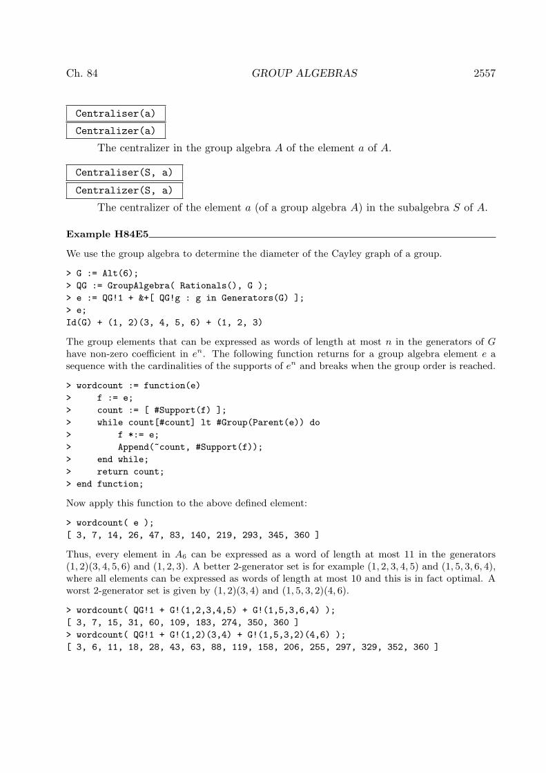
Ch. 84 GROUP ALGEBRAS 2557
Centraliser(a)
Centralizer(a)
The centralizer in the group algebra A of the element a of A.
Centraliser(S, a)
Centralizer(S, a)
The centralizer of the element a (of a group algebra A) in the subalgebra S of A.
Example H84E5
We use the group algebra to determine the diameter of the Cayley graph of a group.
> G := Alt(6);
> QG := GroupAlgebra( Rationals(), G );
> e := QG!1 + &+[ QG!g : g in Generators(G) ];
> e;
Id(G) + (1, 2)(3, 4, 5, 6) + (1, 2, 3)
The group elements that can be expressed as words of length at most n in the generators of Ghave non-zero coefficient in en. The following function returns for a group algebra element e asequence with the cardinalities of the supports of en and breaks when the group order is reached.
> wordcount := function(e)
> f := e;
> count := [ #Support(f) ];
> while count[#count] lt #Group(Parent(e)) do
> f *:= e;
> Append(~count, #Support(f));
> end while;
> return count;
> end function;
Now apply this function to the above defined element:
> wordcount( e );
[ 3, 7, 14, 26, 47, 83, 140, 219, 293, 345, 360 ]
Thus, every element in A6 can be expressed as a word of length at most 11 in the generators(1, 2)(3, 4, 5, 6) and (1, 2, 3). A better 2-generator set is for example (1, 2, 3, 4, 5) and (1, 5, 3, 6, 4),where all elements can be expressed as words of length at most 10 and this is in fact optimal. Aworst 2-generator set is given by (1, 2)(3, 4) and (1, 5, 3, 2)(4, 6).
> wordcount( QG!1 + G!(1,2,3,4,5) + G!(1,5,3,6,4) );
[ 3, 7, 15, 31, 60, 109, 183, 274, 350, 360 ]
> wordcount( QG!1 + G!(1,2)(3,4) + G!(1,5,3,2)(4,6) );
[ 3, 6, 11, 18, 28, 43, 63, 88, 119, 158, 206, 255, 297, 329, 352, 360 ]

2558 ALGEBRAS Part XII
Example H84E6
The group algebra can also be used to investigate the random distribution of words of a certainlength in the generators of the group.
> M11 := sub< Sym(11) | (1,11,9,10,4,3,7,2,6,5,8), (1,5,6,3,4,2,7,11,9,10,8) >;
> A := GroupAlgebra(RealField(16), M11 : Rep := "Vector");
> A;
Group algebra with vector representation
Coefficient ring: Real Field of precision 16
Group: Permutation group M11 acting on a set of cardinality 11
Order = 7920 = 2^4 * 3^2 * 5 * 11
(1, 11, 9, 10, 4, 3, 7, 2, 6, 5, 8)
(1, 5, 6, 3, 4, 2, 7, 11, 9, 10, 8)
> e := (A!M11.1 + A!M11.2) / 2.0;
> eta := Eta(A) / #M11;
For growing n, the words of length n in the generators of M11 converge towards a random distri-bution iff en converges towards eta. We look at the quadratic differences of the coefficients ofen-eta for n = 10, 20, 30, 40, 50.
> e10 := e^10;
> f := A!1;
> for i in [1..5] do
> f *:= e10;
> print &+[ c^2 : c in Eltseq(f - eta) ];
> end for;
0.0012050667195213
1.289719354694155e-5
5.9390965208879e-7
3.394099291966e-8
2.19432454574986e-9

85 BASIC ALGEBRAS85.1 Introduction . . . . . . . . 2563
85.2 Basic Algebras . . . . . . . 2563
85.2.1 Creation . . . . . . . . . . . . 2563
BasicAlgebra(Q) 2563BasicAlgebra(F,R,s,P) 2564BasicAlgebra(F,R) 2564TensorProduct(A, B) 2564BasicAlgebra(G, k) 2564BasicAlgebra(G, k) 2564BasicAlgebra(G) 2564
85.2.2 Special Basic Algebras . . . . . . 2564
BasicAlgebra(A) 2565BasicAlgebraOfMatrixAlgebra(A) 2565BasicAlgebraOfEndomorphismAlgebra(M) 2565BasicAlgebraOfHeckeAlgebra(G, H, F) 2565BasicAlgebraOfSchurAlgebra(n, r, F) 2565BasicAlgebraOfGroupAlgebra(G,F) 2565BasicAlgebraOfGroupAlgebra(G,F) 2565BasicAlgebraOfGroupAlgebra(G,F) 2565BasicAlgebra(S) 2565BasicAlgebraOfBlockAlgebra(S) 2566BasicAlgebraOfPrincipalBlock(G,k) 2566BasicAlgebraOfExtAlgebra(A) 2566BasicAlgebraOfExtAlgebra(A) 2566BasicAlgebraOfExtAlgebra(A) 2566OppositeAlgebra(B) 2566
85.2.3 Access Functions . . . . . . . . 2570
. 2570BaseRing(B) 2570CoefficientRing(B) 2570VectorSpace(B) 2570KSpace(B) 2570Dimension(B) 2570Basis(B) 2570Generators(B) 2570IdempotentGenerators(B) 2570IdempotentPositions(B) 2571NonIdempotentGenerators(B) 2571Random(B) 2571NumberOfProjectives(B) 2571NumberOfGenerators(B) 2571Ngens(B) 2571DimensionsOfProjectiveModules(B) 2571DimensionsOfInjectiveModules(B) 2571
85.2.4 Elementary Operations . . . . . . 2571
+ 2571* 2571^ 2571
85.2.5 Boolean Functions . . . . . . . . 2575
IsDimensionCompatible(B) 2575IsPathTree(B) 2575
IsCommutative(A) 2575IsCentral(A,x) 2575
85.3 Homomorphisms . . . . . . 2575
hom< > 2575Kernel(phi) 2576Image(phi) 2576IsAlgebraHomomorphism(A, B, psi) 2576* 2576IsAlgebraHomomorphism(A, B, psi) 2576IsAlgebraHomomorphism(A, B, psi) 2576IsAlgebraHomomorphism(A, B, psi) 2576IsAlgebraHomomorphism(A, B, psi) 2576IsAlgebraHomomorphism(psi) 2576
85.4 Subalgebras and Quotient Alge-bras . . . . . . . . . . . . 2576
85.4.1 Subalgebras and their Constructions 2576
sub< > 2576SubalgebraFromBasis(A, V) 2576MaximalIdempotent(A, S) 2577MinimalIdentity(A, S) 2577Centre(A) 2577Centralizer(A,S) 2577MaximalCommutativeSubalgebra(A,S) 2577
85.4.2 Ideals and their Construction . . . 2577
ideal< > 2577ideal< > 2577LeftAnnihilator(A, S) 2577RightAnnihilator(A, S) 2577Annihilator(A,S) 2577IsIdeal(A, S) 2577IsLeftIdeal(A,S) 2578IsRightIdeal(A, S) 2578RandomIdealGeneratedBy(A, n) 2578
85.4.3 Quotient Algebras . . . . . . . . 2578
quo< > 2578CoverAlgebra(A) 2578GradedCoverAlgebra(A) 2578TruncatedAlgebra(A,n) 2578
85.5 Minimal Forms and Gradings . 2579
MinimalGeneratorForm(A) 2579MinimalGeneratorFormAlgebra(A) 2579AssociatedGradedAlgebra(A) 2579GradedCapHomomorphism(A) 2579GradedCapHomomorphism(A, B, mu) 2579BuildHomomorphismFromGraded
Cap(A, B, phi) 2579ChangeIdempotents(A, S) 2579ChangeIdempotents(A, S) 2579
85.6 Automorphisms and Isomorphisms2581

2560 ALGEBRAS Part XII
GradedAutomorphismGroupMatchingIdempotents(A) 2581
GradedAutomorphismGroup(A) 2581IsGradedIsomorphic(A, B) 2581AutomorphismGroupMatching
Idempotents(A) 2581AutomorphismGroup(A) 2582IsIsomorphic(A, B) 2582
85.7 Modules over Basic Algebras . 2583
85.7.1 Indecomposable Projective Modules 2583
ProjectiveModule(B, i) 2583PathTree(B, i) 2583ActionGenerator(B, i) 2584IdempotentActionGenerators(B, i) 2584NonIdempotentActionGenerators(B, i) 2584Injection(B, i, v) 2584
85.7.2 Creation . . . . . . . . . . . . 2584
AModule(B, Q) 2584ProjectiveModule(B, S) 2584IrreducibleModule(B, i) 2584SimpleModule(B, i) 2584ZeroModule(B) 2584RightRegularModule(B) 2584RegularRepresentation(v) 2585Restriction(M, B, xi) 2585ChangeAlgebra(M, B, xi) 2585ChangeAlgebra(M, B, xi) 2585JacobsonRadical(M) 2585Socle(M) 2585
85.7.3 Access Functions . . . . . . . . 2585
Algebra(M) 2585Dimension(M) 2585Action(M) 2585IsomorphismTypesOfRadicalLayers(M) 2585IsomorphismTypesOfSocleLayers(M) 2585IsomorphismTypesOfBasicAlgebra
Sequence(S) 2585
85.7.4 Predicates . . . . . . . . . . . 2587
IsSemisimple(M) 2587IsProjective(M) 2588IsInjective(M) 2588
85.7.5 Elementary Operations . . . . . . 2588
* 2588
85.8 Homomorphisms of Modules . 2590
85.8.1 Creation . . . . . . . . . . . . 2590
AHom(M, N) 2590PHom(M,N) 2590ZeroMap(M, N) 2590LiftHomomorphism(x, n) 2590LiftHomomorphism(X, N) 2591Pushout(M, f1, N1, f2, N2) 2591Pullback(f1, M1, f2, M2, N) 2591
85.8.2 Access Functions . . . . . . . . 2591
IsModuleHomomorphism(f) 2591Domain(f) 2591Codomain(f) 2591Kernel(f) 2591Cokernel(f) 2591
85.8.3 Projective Covers and Resolutions . 2592
ProjectiveCover(M) 2592ProjectiveResolution(M, n) 2592CompactProjectiveResolution(M, n) 2593CompactProjectiveResolutionsOf
SimpleModules(A,n) 2593SyzygyModule(M, n) 2593SimpleHomologyDimensions(M) 2593
85.9 Duals and Injectives . . . . . 2596
Dual(M) 2596BaseChangeMatrix(A) 2596
85.9.1 Injective Modules . . . . . . . . 2597
InjectiveModule(B, i) 2597InjectiveHull(M) 2597InjectiveResolution(M, n) 2597CompactInjectiveResolution(M, n) 2597InjectiveSyzygyModule(M, n) 2598SimpleCohomologyDimensions(M) 2598
85.10 Cohomology . . . . . . . 2600
CohomologyRingGenerators(P) 2600CohomologyRightModule
Generators(P, Q, CQ) 2600CohomologyLeftModule
Generators(P, CP, Q) 2601DegreesOfCohomologyGenerators(C) 2601CohomologyGenerator
ToChainMap(P, Q, C, n) 2601CohomologyGeneratorTo
ChainMap(P, C, n) 2601
85.10.1 Ext-Algebras . . . . . . . . . 2605
ExtAlgebra(A, n) 2605BasicAlgebraOfExtAlgebra(ext) 2606BasicAlgebraOfExtAlgebra(A) 2606BasicAlgebraOfExtAlgebra(A, n) 2606SumOfBettiNumbersOfSimple
Modules(A, n) 2606
85.11 Group Algebras of p-groups . 2607
85.11.1 Access Functions . . . . . . . 2608
Group(A) 2608PCGroup(A) 2608PCMap(A) 2608AModule(M) 2608GModule(M) 2608GModule(M) 2608
85.11.2 Projective Resolutions . . . . . 2608
ResolutionData(A) 2608CompactProjectiveResolution
PGroup(M, n) 2608CompactProjectiveResolution(M, n) 2608

Ch. 85 BASIC ALGEBRAS 2561
ProjectiveResolutionPGroup(PR) 2609ProjectiveResolution(M, n) 2609ProjectiveResolution(PR) 2609
85.11.3 Cohomology Generators . . . . 2609
AllCompactChainMaps(PR) 2609CohomologyElementToChainMap(P, d, n) 2609CohomologyElementToCompact
ChainMap(PR, d, n) 2609
85.11.4 Cohomology Rings . . . . . . 2610
CohomologyRing(k, n) 2610CohomologyRing(PR, AC) 2610MinimalRelations(R) 2610
85.11.5 Restrictions and Inflations . . . 2610
RestrictionData(A,B) 2610RestrictResolution(PR, RD) 2610RestrictionChainMap(P1,P2) 2610RestrictionOfGenerators(PR1, PR2, AC1,
AC2, REL2) 2611
InflationMap(PR2, PR1, AC2, AC1,REL1, theta) 2611
85.12 A-infinity Algebra Structureson Group Cohomology . . . 2614
AInfinityRecord(G,n) 2614MasseyProduct(Aoo,terms) 2615HighProduct(Aoo,terms) 2615HighMap(Aoo,terms) 2615
85.12.1 Homological Algebra Toolkit . . 2616
ActionMatrix(A,x) 2616CohomologyRingQuotient(CR) 2616LiftToChainmap(P,f,d) 2616NullHomotopy(f) 2616IsNullHomotopy(f,H) 2616ChainmapToCohomology(f,CR) 2616CohomologyToChainmap(xi,CR,P) 2616
85.13 Bibliography . . . . . . . 2618


Chapter 85
BASIC ALGEBRAS
85.1 Introduction
A basic algebra is a finite dimensional algebra A over a field, all of whose simple moduleshave dimension one. In the literature such an algebra is known as a “split” basic algebra.Every algebra is Morita equivalent to a basic algebra, though a field extension may benecessary to obtain the split basic algebra. Magma has several functions that create thebasic algebras corresponding to algebras of different types.
The type AlgBas in Magma is optimized for the purposes of doing homological calcu-lations. A basic algebra A is generated by elements a1, a2, . . . , at where a1, . . . , as are theprimitive idempotent generators and as+1, . . . , at are the nonidempotent generators. Eachnonidempotent generator, ak must have the property that ai ∗ ak ∗ aj = ak for specificidempotent generators ai and aj . The projective indecomposable modules have the formPi = ai ·A for i = 1, . . . , s and the simple modules have the form Si = Pi/Rad(Pi), whereRad(Pi) is the radical of Pi.
85.2 Basic Algebras
In the Magma implementation the algebra is given as the sequence of projective modulesP1, . . . , Ps together with a path tree for each projective module. A projective moduleconsists of a matrix for each generator a1, a2, . . . , at giving the action of the generator onthe vector space of the module. The basis b1, b2, . . . , bn for the vector space of Pi is chosen sothat each basis element is the image of a basis element of lower index under multiplicationby a nonidempotent generator of A. The structure of the basis is recorded in the path treewhich is a sequence [< 1, i >,< j, k >, . . .] of 2-tuples of length n = Dimension(Pi). Thefirst entry < 1, i > indicates that b1 = b1 ∗ ai where ai is the primitive idempotent in thealgebra A such that Pi = A · ai. Similarly, if entry number k in the path tree is 〈u, v〉 thenbk = bu ∗ av where v > s if k > 1.
85.2.1 CreationThe first function for creating a basic algebra is the most basic, in which the user suppliesthe projective modules and the path trees directly.
BasicAlgebra(Q)
Given a sequence [Qi, . . . , Qs] of 2-tuples such that each Qi =< Mi, Ti > consistingof a module for a matrix algebra Mi and a path tree Ti for Mi, the function createsthe basic algebra whose projective modules are the first entries M1, . . . ,Ms and thepath trees are the corresponding second entries.

2564 ALGEBRAS Part XII
The next two functions create a basic algebra from generators and relations. Theuser must, additionally, specify the quiver with relations, giving the number ofidempotents and the beginning and end points of the arrows in the quiver.
BasicAlgebra(F,R,s,P)
Creates the basic algebra given by the presentation. Here F is a free algebra andR is the sequence of relation for the nonidempotent generators of the algebra. Ifthe free algebra F is generated by elements a1, . . . , at, the function assumes thata1, . . . , as are the mutually orthogonal primitive idempotents and it creates all of theappropriate relations including a1 + . . .+as = 1. The nonidempotent generators arethen as+1, . . . , at. So `k = 〈i, j〉 for i, j ≤ s means that as+k = ai ∗ as+k ∗ aj . Eachof the relations in R is given as a linear combination of words in the nonidempotentgenerators as+1, . . . , at ∈ F . The sequence P is a sequence of 2-tuples, one for eachnonidempotent generator, giving the beginning and ending nodes of the generator.That is, each tuple is the pair of indices of the idempotents which multiply as theidentity on the nonidempotent generator on the left and on the right.
BasicAlgebra(F,R)
Creates the basic algebra of a local algebra from the presentation of the algebra.Here F is a free algebra whose variable represent the nonidempotent generators andR is the sequence of relations among those variables.
TensorProduct(A, B)
The tensor product of the basic algebras A and B.The modular group algebra of a p-group is naturally a basic algebra. The nextfunction create the basic algebra from the group information.
BasicAlgebra(G, k)
BasicAlgebra(G, k)
BasicAlgebra(G)
Given a finite p-group G and a finite field k of characteristic p, returns the groupalgebra kG in the form of a basic algebra. If no field k is supplied then the primefield of characteristic p is assumed to be the field of coefficients.
85.2.2 Special Basic AlgebrasThere are several functions that create basic algebras of special interest. The most basic ofthese creates the basic algebra that is Morita equivalent to a matrix algebra defined overa finite field by first condensing the algebra and then splitting the irreducible modules asneeded.
Included among these constructions are the basic algebras of Schur algebras and Heckealgebras over finite fields. The Schur algebras arise in the representation theory of symmet-ric groups. The Schur algebras have finite global dimension and hence their ext-algebrashave finite dimension. By a Hecke algebra, we mean the algebra of endomorphisms of apermutation module of a finite group.
Ch. 85 BASIC ALGEBRAS 2565
BasicAlgebra(A)
BasicAlgebraOfMatrixAlgebra(A)
This function creates the split basic algebra of the matrix algebra A. The functionfirst produces a presentation and condensed algebra for A. In the event that thefield of coefficients k of A is not a splitting field, then the returned basic algebra isdefined over the minimal extension of k that is a splitting field for A.
BasicAlgebraOfEndomorphismAlgebra(M)
Returns the split basic algebra of the endomorphism ring of the module M . In theevent that the field of coefficients of M is not a splitting field for M , then the fieldis extended and the basic algebra is defined over the minimal extension needed tosplit M .
BasicAlgebraOfHeckeAlgebra(G, H, F)
Returns the basic algebra of the Hecke algebra which is the algebra of endomor-phisms of the permutation module over G with point stabilizer H and field of coef-ficients F . In the event that F is not a splitting field then the field F is extendedto a splitting field which is the field of coefficients of the returned basic algebra.
BasicAlgebraOfSchurAlgebra(n, r, F)
Creates the basic algebra of the Schur algebra S(n, r) over the field F . The Schuralgebra is the algebra of endomorphisms of the module over the symmetric groupSym(r) that is the tensor product of r copies of a vector space V over F of dimensionn, the group Sym(r) acting by permuting the r copies.
BasicAlgebraOfGroupAlgebra(G,F)
BasicAlgebraOfGroupAlgebra(G,F)
BasicAlgebraOfGroupAlgebra(G,F)
The function returns the basic algebra of the group algebra of G with coefficientsin the field F . The function requires the creation of the projective indecomposableFG-modules. In the event that the field F is not a splitting field for the irreducibleFG-modules then the base ring of the returned algebra is the minimal extension ofF that is necessary to get a splitting field.
BasicAlgebra(S)
Returns the basic algebra of the action algebra on the module which is the directsum of the modules in the sequence S. In the event that the irreducible compositionfactors of the modules in S are not absolutely irreducible, then the returned basicalgebra is defined over the splitting field for the irreducible modules.

2566 ALGEBRAS Part XII
BasicAlgebraOfBlockAlgebra(S)
Returns the basic algebra of the block algebra, the projective modules of which aregiven in the sequence S. In the event that the irreducible composition factors ofthe modules in S are not absolutely irreducible, then the returned basic algebra isdefined over the splitting field for the irreducible modules.
BasicAlgebraOfPrincipalBlock(G,k)
Returns the basic algebra of the principal block of the group algebra of G. Ifthe simple modules in the principal kG block are all absolutely simple, then theordering of the projective modules for the returned basic algebra is exactly the sameas the ordering of the projectives modules in the principal block returned by thefunction IndecomposableProjectives. Otherwise, the base ring of the returnedbasic algebra is the least extension of k necessary to split the simple modules inthe principal block and the simple modules of the returned algebra are ordered byincreasing dimension of the corresponding simple modules of kG.
BasicAlgebraOfExtAlgebra(A)
The function returns the basic algebra from a computed ext-algebra which isExt∗A(S, S), where S is the direct sum of the irreducible A-modules, of the basicalgebra A. If no ext-algebra for A has been computed or if the exalgebra is notverified to be finite dimensional then an error is returned.
BasicAlgebraOfExtAlgebra(A)
The function returns the basic algebra for the ext-algebra, which is Ext∗A(S, S),where S is the direct sum of the irreducible A-modules, of A computed to n steps.If no ext-algebra for A to n steps has been computed then it will be computed. Ifthe ext-algebra is not verified to be finite dimensional by the computation, then anerror is returned.
BasicAlgebraOfExtAlgebra(A)
The function creates the basic algebra from a computed ext-algebra. The input extis the output of the ExtAlgebra function. If the ext-algebra is not verified to befinite dimensional by the computation, then an error is returned.
OppositeAlgebra(B)
The opposite algebra of the basic algebra B. The opposite algebra of B is the algebrawith the same set of elements and the same addition but with multiplication ∗ givenby a ∗ b = ba for a and b in A.

Ch. 85 BASIC ALGEBRAS 2567
Example H85E1
We form the basic algebra of the group algebra of the alternating group on 6 letters in characteristic2.
> G := AlternatingGroup(6);
> A := BasicAlgebraOfGroupAlgebra(G, GF(2));
> A;
Basic algebra of dimension 36 over GF(2^2)
Number of projective modules: 5
Number of generators: 9
Note that the field of coefficients has been extended in order to split the irreducible G-modules. Agreat deal of information on the nature of the group algebra and its basic algebra can be obtainedfrom analysis such as the following.
> [Dimension(ProjectiveModule(A,i)): i in [1 .. 5]];
[ 9, 9, 16, 1, 1 ]
> prj := CompactProjectiveResolutionsOfAllSimpleModules(A,8);
> [x‘BettiNumbers:x in prj];
[
[
[ 1, 0, 0, 0, 0 ],
[ 0, 0, 1, 0, 0 ],
[ 1, 0, 0, 0, 0 ],
[ 1, 0, 0, 0, 0 ],
[ 0, 0, 1, 0, 0 ],
[ 1, 0, 0, 0, 0 ],
[ 1, 0, 0, 0, 0 ],
[ 0, 0, 1, 0, 0 ],
[ 1, 0, 0, 0, 0 ]
],
[
[ 0, 1, 0, 0, 0 ],
[ 0, 0, 1, 0, 0 ],
[ 0, 1, 0, 0, 0 ],
[ 0, 1, 0, 0, 0 ],
[ 0, 0, 1, 0, 0 ],
[ 0, 1, 0, 0, 0 ],
[ 0, 1, 0, 0, 0 ],
[ 0, 0, 1, 0, 0 ],
[ 0, 1, 0, 0, 0 ]
],
[
[ 0, 0, 3, 0, 0 ],
[ 1, 1, 2, 0, 0 ],
[ 0, 0, 3, 0, 0 ],
[ 0, 0, 2, 0, 0 ],
[ 1, 1, 1, 0, 0 ],
[ 0, 0, 2, 0, 0 ],

2568 ALGEBRAS Part XII
[ 0, 0, 1, 0, 0 ],
[ 1, 1, 0, 0, 0 ],
[ 0, 0, 1, 0, 0 ]
],
[
[ 0, 0, 0, 0, 0 ],
[ 0, 0, 0, 0, 0 ],
[ 0, 0, 0, 0, 0 ],
[ 0, 0, 0, 0, 0 ],
[ 0, 0, 0, 0, 0 ],
[ 0, 0, 0, 0, 0 ],
[ 0, 0, 0, 0, 0 ],
[ 0, 0, 0, 0, 0 ],
[ 0, 0, 0, 1, 0 ]
],
[
[ 0, 0, 0, 0, 0 ],
[ 0, 0, 0, 0, 0 ],
[ 0, 0, 0, 0, 0 ],
[ 0, 0, 0, 0, 0 ],
[ 0, 0, 0, 0, 0 ],
[ 0, 0, 0, 0, 0 ],
[ 0, 0, 0, 0, 0 ],
[ 0, 0, 0, 0, 0 ],
[ 0, 0, 0, 0, 1 ]
]
]
So we see that the last two simple modules are projective and hence in the group algebra FG,they represent blocks of defect 0. From the information on the Betti numbers we observe that thefirst two simple modules have periodic projective resolutions. Thus the third simple module forthe basic algebra corresponds to the trivial FG-module, which we know is neither projective norperiodic.
Example H85E2
We construct the Schur algebra S(3, 7) with coefficients in a field of characteristic 2.
> A := BasicAlgebraOfSchurAlgebra(3,6,GF(2));
> A;
Basic algebra of dimension 58 over GF(2)
Number of projective modules: 7
Number of generators: 21
It is known that A has finite global dimension, hence its ext-algebra has finite dimension.
> B := BasicAlgebraOfExtAlgebra(A,10);
> B;
Basic algebra of dimension 56 over GF(2)
Number of projective modules: 7

Ch. 85 BASIC ALGEBRAS 2569
Number of generators: 25
We check to see if the ext-algebra of B might have finite dimension.
> SumOfBettiNumbersOfSimpleModules(B,5);
600
> SumOfBettiNumbersOfSimpleModules(B,6);
1334
> SumOfBettiNumbersOfSimpleModules(B,7);
3008
The sum of the Betti number would be the dimension of the ext-algebra computed to the indicateddegree. It would appear that the ext-algebra is infinite dimensional. Just to check, we look at aparticular simple module, chosen randomly.
> CompactProjectiveResolution(SimpleModule(B,4),10)‘BettiNumbers;
[
[ 8, 0, 81, 3, 61, 69, 55 ],
[ 3, 0, 36, 1, 26, 30, 24 ],
[ 1, 0, 16, 1, 11, 13, 10 ],
[ 1, 0, 7, 1, 5, 5, 4 ],
[ 1, 0, 3, 1, 2, 2, 1 ],
[ 1, 0, 1, 0, 1, 1, 0 ],
[ 0, 0, 0, 0, 1, 1, 0 ],
[ 0, 0, 0, 0, 1, 0, 1 ],
[ 0, 0, 0, 1, 0, 1, 0 ],
[ 1, 0, 0, 0, 0, 0, 1 ],
[ 0, 0, 0, 1, 0, 0, 0 ]
]
Thus we have strong evidence that the fourth simple module has infinite projective dimension. Inthat case, the ext-algebra of B is not finite dimensional.Now we consider the same example except in characteristic 3.
> A := BasicAlgebraOfSchurAlgebra(3,6,GF(3));
> A;
Basic algebra of dimension 48 over GF(3)
Number of projective modules: 7
Number of generators: 21
> B := BasicAlgebraOfExtAlgebra(A,10);
> B;
Basic algebra of dimension 98 over GF(3)
Number of projective modules: 7
Number of generators: 21
> SumOfBettiNumbersOfSimpleModules(B,5);
48
> SumOfBettiNumbersOfSimpleModules(B,6);
48
So we see that the algebra B has global dimension at most 5. We can compute its ext-algebra.
> C := BasicAlgebraOfExtAlgebra(B,10);

2570 ALGEBRAS Part XII
> C;
Basic algebra of dimension 48 over GF(3)
Number of projective modules: 7
Number of generators: 21
> D := BasicAlgebraOfExtAlgebra(C,10);
> D;
Basic algebra of dimension 98 over GF(3)
Number of projective modules: 7
Number of generators: 21
This provides evidence that A is isomorphic to its double ext-algebra. This would suggest that Amight be a Koszul algebra.
85.2.3 Access FunctionsThese functions return basic information, underlying structures and elements of the givenbasic algebras.
B . i
The ith element in the standard basis for the underlying vector space of the algebraB.
BaseRing(B)
CoefficientRing(B)
Given an algebra B over a field k the function returns k.
VectorSpace(B)
KSpace(B)
The underlying k-vector space of the algebra B. The space is the direct sum of theunderlying vector space of the indecomposable projective modules.
Dimension(B)
The dimension of the underlying vector space of the algebra B.
Basis(B)
A basis of the underlying vector space of the algebra B.
Generators(B)
The generators of the algebra B as a sequence of elements in the underlying vectorspace of the algebra B.
IdempotentGenerators(B)
The sequence of mutually orthogonal idempotent generators of the basic algebra Bas elements in the underlying vector space of B.

Ch. 85 BASIC ALGEBRAS 2571
IdempotentPositions(B)
The sequenceN = [n1, . . . , ns] such that B.n1, . . . , B.ns are the mutually orthogonalidempotent generators of the algebra B.
NonIdempotentGenerators(B)
The sequence of nonidempotent generators of the basic algebra B as elements in theunderlying vector space of the algebra B.
Random(B)
A random element of the algebra B as an element of the underlying vector space ofB.
NumberOfProjectives(B)
The number of nonisomorphic indecomposable projective modules in the basic al-gebra B.
NumberOfGenerators(B)
Ngens(B)
The number of generators (idempotent and nonidempotent) of the basic algebra B.
DimensionsOfProjectiveModules(B)
The sequence of the dimensions of the projective modules of the basic algebra B.
DimensionsOfInjectiveModules(B)
The sequence of the dimensions of the injective modules of the basic algebra B.
85.2.4 Elementary Operations
a + b
The sum of the two elements a and b.
a * b
The product of the two elements a and b.
a ^ n
The nth power of the element a.

2572 ALGEBRAS Part XII
Example H85E3
We create the basic algebra of the quiver with three nodes and three arrows over the field with 7elements. The first arrow (a) goes from node 1 to node 2, the second (b) from node 2 to node 1,and (c) from node 2 to node 3. The arrows satisfy the relation that (a ∗ b)3 = 0.
> ff := GF(7);
> FA<e1,e2,e3,a,b,c> := FreeAlgebra(ff,6);
> rrr := [a*b*a*b*a*b];
> D := BasicAlgebra(FA,rrr,3,[<1,2>,<2,1>,<2,3>]);
> D;
Basic algebra of dimension 21 over GF(7)
Number of projective modules: 3
Number of generators: 6
> DimensionsOfProjectiveModules(D);
[ 9, 11, 1 ]
> DimensionsOfInjectiveModules(D);
[ 6, 7, 8 ]
So we can see that the algebra is not self-injective.Now we can check the nilpotence degree of the radical of D. The radical of D is generated by thenonidempotent generators.
> S := NonIdempotentGenerators(D);
> S;
[ (0 1 0 0 0 0 0 0 0 0 0 0 0 0 0 0 0 0 0 0 0), (0 0 0 0 0 0 0 0 0 0 1 0 0 0 0 0
0 0 0 0 0), (0 0 0 0 0 0 0 0 0 0 0 1 0 0 0 0 0 0 0 0 0) ]
> S2 := [x*y:x in S, y in S|x*y ne 0];
> #S2;
3
> S3 := [x*y:x in S2, y in S|x*y ne 0];
> #S3;
3
> S4 := [x*y:x in S3, y in S|x*y ne 0];
> #S4;
3
> S5 := [x*y:x in S4, y in S|x*y ne 0];
> #S5;
3
> S6 := [x*y:x in S5, y in S|x*y ne 0];
> #S6;
2
> S7 := [x*y:x in S6, y in S|x*y ne 0];
> #S7;
1
> S8 := [x*y:x in S7, y in S|x*y ne 0];
> #S8;
0

Ch. 85 BASIC ALGEBRAS 2573
Example H85E4
First we create the basic algebra for the symmetric group S3 over the field GF (3)
> FA<e1,e2,a,b> := FreeAlgebra(GF(3),4);
> MM:= [a*b*a, b*a*b];
> BS3 := BasicAlgebra(FA, MM, 2, [<1,2>,<2,1>]);
> BS3;
Basic algebra of dimension 6 over GF(3)
Number of projective modules: 2
Number of generators: 4
> DimensionsOfProjectiveModules(BS3);
[ 3, 3 ]
Next we create the basic algebra for the cyclic group of order 3.
> gg := CyclicGroup(3);
> BC3 := BasicAlgebra(gg,GF(3));
> BC3;
Basic algebra of dimension 3 over GF(3)
Number of projective modules: 1
Number of generators: 2
We create the basic algebra for the direct product C3 × S3.
> A := TensorProduct(BS3,BC3);
> A;
Basic algebra of dimension 18 over GF(3)
Number of projective modules: 2
Number of generators: 6
> DimensionsOfProjectiveModules(A);
[ 9, 9 ]
Example H85E5
We create the basic algebra for A4 over a field with 2 elements. The group algebra has twononisomorphic projective modules. We define the basic algebra by constructing the matrix algebrafor the projective modules and the path trees and entering this data into the BasicAlgebra
function.Note that the matrices are sparse so we will define them by specifying the nonzero rows.
> ff := GF(2);
> MM6 := MatrixAlgebra(ff,6);
> e11 := MM6!0;
> e12 := MM6!0;
> VV6 := VectorSpace(GF(2),6);
> BB6 := Basis(VV6);
> e11[1] := BB6[1];
> e11[3] := BB6[3];
> e11[4] := BB6[4];
> e11[6] := BB6[6];

2574 ALGEBRAS Part XII
> e12[2] := BB6[2];
> e12[5] := BB6[5];
> a1 := MM6!0;
> b1 := MM6!0;
> c1 := MM6!0;
> d1 := MM6!0;
> a1[1] := BB6[2];
> b1[1] := BB6[3];
> c1[2] := BB6[4];
> a1[3] := BB6[5];
> b1[4] := BB6[6];
> c1[5] := BB6[6];
> A1 := sub< MM6 | [e11, e12, a1, b1, c1, d1] >;
> T1 := [ <1,1>, <1,3>, <1,4>, <2,5>, <3,3>, <4,4>];
>
> VV5 := VectorSpace(ff,5);
> BB5 := Basis(VV5);
> MM5 := MatrixAlgebra(ff,5);
> e21 := MM5!0;
> e22 := MM5!0;
> e22[1] := BB5[1];
> e22[3] := BB5[3];
> e22[5] := BB5[5];
> e21[2] := BB5[2];
> e21[4] := BB5[4];
> a2 := MM5!0;
> b2 := MM5!0;
> c2 := MM5!0;
> d2 := MM5!0;
> f2 := MM5!0;
> g2 := MM5!0;
> c2[1] := BB5[2];
> d2[1] := BB5[3];
> b2[2] := BB5[4];
> d2[3] := BB5[5];
> a2[4] := BB5[5];
> A2 := sub< MM5 | [e21, e22, a2, b2, c2, d2] >;
> T2 := [<1,2>, <1,5>, <1,6>, <2,4>, <3,6>];
>
> C := BasicAlgebra( [<A1, T1>, <A2, T2>] );
> C;
Basic algebra of dimension 11 over GF(2)
Number of projective modules: 2
Number of generators: 6
> DimensionsOfProjectiveModules(C);
[ 6, 5 ]
> DimensionsOfInjectiveModules(C);

Ch. 85 BASIC ALGEBRAS 2575
[ 6, 5 ]
85.2.5 Boolean FunctionsA basic algebra in Magma is a sequence of matrix algebras, each with a path tree. Whena basic algebra is created by entering such a sequence, Magma does not check to see ifall of the properties of a basic algebra are satisfied, as this is an expensive operation. Thefollowing two function check to see if the properties of a basic algebra are satisfied.
IsDimensionCompatible(B)
Returns true if the dimension of a basic algebra is the same as the dimension of thematrix algebra of its action on itself. If false then the algebra is not a basic algebra.
IsPathTree(B)
Returns true if the basis elements of the projective modules in the basic algebra aredetermined by the path tree. If false, then the algebra is not a true basic algebra.Two other functions check commutativity.
IsCommutative(A)
Returns true if the basic algebra A is commutative.
IsCentral(A,x)
Returns true if the element x is in the center of the basic algebra A.
85.3 Homomorphisms
Magma has the capability of creating homomorphisms of basic algebras. A homomorphismof a basic algebra has the type Map. The matrix of the homomorphism φ is accessed byentering Matrix(phi). The kernel of a homomorphism is returned as a subspace of thevector space of the domain of the algebra. This is a two-sided ideal. There is no specialtype for ideals. They are subspaces of the underlying vector space of the algebra. Theycan be generated from any given set of elements of the algebra
The image of a homomorphism is returned as a basic algebra, together with the em-bedding homomorphism.
A homomorphism from a basic algebra A to a basic algebra B is normally created froma matrix having dimension of A rows and dimension of B columns. Note that Magmadoes not automatically check to see if the created map is an algebra homomorphism.
hom< A - >
The algebra homomorphism from basic algebra A to basic algebra B, whose matrixis the matrix S. Given a map φ, a homomorphism of basic algebra, the matrix ofthat map is recalled with the command Matrix(phi).

2576 ALGEBRAS Part XII
Kernel(phi)
The kernel of the map φ.
Image(phi)
The image of the homomorphism φ together with the embedding homomorphism ofthe image into the codomain of φ.
IsAlgebraHomomorphism(A, B, psi)
Return true if the matrix ψ represents a homomorphism from basic algebra A tobasic algebra B.
X * Y
The composition of the maps X and Y .
IsAlgebraHomomorphism(A, B, psi)
IsAlgebraHomomorphism(A, B, psi)
IsAlgebraHomomorphism(A, B, psi)
IsAlgebraHomomorphism(A, B, psi)
Returns true, if the map ψ is a homomorphism of basic algebras
IsAlgebraHomomorphism(psi)
Returns true if the map ψ is a homomorphism of basic algebras.
85.4 Subalgebras and Quotient Algebras
A subalgebra is also returned with the embedding homomorphism, and a quotient algebrais returned with the natural quotient map. These are needed for creating some standardsubalgebras such as the centre of the algebra.
85.4.1 Subalgebras and their Constructions
sub< A | S >
The subalgebra of A generated by the elements of the sequence S, together with theinclusion map of the subalgebra into A. The subalgebra contains the idempotent ofminimal rank in A that acts as a multiplicative identity on the elements of S.
SubalgebraFromBasis(A, V)
Given a basic algebra A and the basis V of a subspace of A, the function returnsthe basic algebra which is the subalgebra spanned by the subspace and the inclusionmatrix of the homomorphism embedding the subalgebra into A. Note that the spaceV might not contain the identity element of V and in that case the minimal possibleidentity element is added to the returned subalgebra.

Ch. 85 BASIC ALGEBRAS 2577
MaximalIdempotent(A, S)
Given a basic algebra A, a subspace S of the vector space of A that is closed undermultiplication, this function returns an idempotent in A which has maximal rankamong all idempotents contained in S.
MinimalIdentity(A, S)
Returns the idempotent of smallest rank that is a two sided identity for the elementsin the set S.
Centre(A)
The centre of the basic algebra as a basic algebra together with the inclusion homo-morphism.
Centralizer(A,S)
Returns the centralizer in the basic algebra A of the elements in the sequence S,along with the homomorphism embedding the centralizer into A.
MaximalCommutativeSubalgebra(A,S)
Returns a maximal commutative subalgebra of the basic algebra A that contains theelements of the sequence S. An error occurs if the elements of S do not commute.
85.4.2 Ideals and their Construction
ideal< A | S >
ideal< A | S >
Returns the subspace of the vector space of the algebra A that is the ideal of the Agenerated by the given sequence of elements S.
LeftAnnihilator(A, S)
Returns a basis for the left annihilator of the sequence S of elements in the basicalgebra A.
RightAnnihilator(A, S)
Returns a basis for the right annihilator of the sequence S of elements in the basicalgebra A.
Annihilator(A,S)
Returns a basis for the two-sided annihilator of the sequence of elements S of thebasic algebra A.
IsIdeal(A, S)
Returns true if the subspace spanned by the elements of S is a two-sided ideal ofthe basic algebra A.

2578 ALGEBRAS Part XII
IsLeftIdeal(A,S)
Returns true if the subspace spanned by the elements of S is a left ideal of the basicalgebra A.
IsRightIdeal(A, S)
Returns true if the subspace spanned by the elements of S is a two-sided ideal ofthe basic algebra A.
RandomIdealGeneratedBy(A, n)
Returns the ideal generated by n randomly selected elements in the Jacobson radicalof the basic algebra A.
85.4.3 Quotient Algebras
quo< A | S >
Returns the quotient algebra of A by the ideal S, which is a subspace of the vectorspace of A, together with the quotient map.
CoverAlgebra(A)
Constructs the maximal extension B as in [0 → K → B → A → 0] such that Bacts trivially on K and B is an algebra with exactly the same minimal number ofgenerators as A. Returns B and the algebra homomorphism of B onto A.
GradedCoverAlgebra(A)
This assumes that we are given the truncated algebra of a graded algebra. It createsthe basic algebra of the natural cover of A and also returns the matrix of the coveronto A.
TruncatedAlgebra(A,n)
The quotient of the algebra by the nth power of the radical of A. Returns also thequotient map.

Ch. 85 BASIC ALGEBRAS 2579
85.5 Minimal Forms and GradingsThere are some standard ways of rewriting an algebra to an isomorphic form. We canalso constructed the associated graded algebra of a basic algebra. Also included here is afunction for rearranging the orders of idempotents in a basic algebra.
The first intrinsic is used extensively in the programs for computing automorphismsand isomorphisms.
MinimalGeneratorForm(A)
Returns a record consisting of an isomorphic basic algebra having the property thatit is generated by a minimal number of elements and the projective modules arefiltered by radical layers. The record consists of the following fields:(a) The algebra in minimal form (field algebra).(b) The map from the minimal generator form algebra to A (field Homomorphism).(c) The inverse map from A to the minimal generator form algebra (field
InverseHomomorphism).(d) The dimensions of the radical layer (field RadicalDimensions).(e) The dimensions of the filtration of the top radical layer by the socle layer (field
FilterDimensions).
MinimalGeneratorFormAlgebra(A)
Returns an isomorphic algebra having minimal generator form.
AssociatedGradedAlgebra(A)
Returns the basic algebra that is isomorphic to the associated graded algebra of A.
GradedCapHomomorphism(A)
Returns the matrix of the map from A/Rad(A) to X/Rad(X) where X is the asso-ciated graded algebra of A.
GradedCapHomomorphism(A, B, mu)
Given an algebra homomorphism mu : A→ B, returns the induced homomorphismA/Rad2(A) → B/Rad2(B), where Rad2 is the second power of the Jacobson radical.
BuildHomomorphismFromGradedCap(A, B, phi)
Returns the graded homomorphism from the associated graded algebra X of A tothe associated graded algebra Y of B, whose cap is φ. That is phi is the matrix ofthe induced homomorphism of X/Rad2(X) to Y/Rad2(Y ).
ChangeIdempotents(A, S)
ChangeIdempotents(A, S)
Returns the basic algebra isomorphic to A, obtained by permuting the order of theidempotents by the permutation S. The permutation S can be given as an elementof the symmetric group or as the sequence of images of the permutation.

2580 ALGEBRAS Part XII
Example H85E6
In this examples we investigate properties of the basic algebra of a Schur algebra.
> A := BasicAlgebraOfSchurAlgebra(3,6,GF(3));
> A;
Basic algebra of dimension 48 over GF(3)
Number of projective modules: 7
Number of generators: 21
> B := BasicAlgebraOfExtAlgebra(A,10);
> B;
Basic algebra of dimension 98 over GF(3)
Number of projective modules: 7
Number of generators: 21
> C := BasicAlgebraOfExtAlgebra(B,10);
> C;
Basic algebra of dimension 48 over GF(3)
Number of projective modules: 7
Number of generators: 21
> boo,mat := IsIsomorphic(A,C);
> boo;
true
> IsAlgebraHomomorphism(mat);
true
So we see that A is isomorphic to its double ext-algebra, and it is graded since the double ext-algebra is graded. Thus we know that the basic algebra A is a Koszul algebra.
Example H85E7
Here we see how to rearrange an algebra by changing the ordering on the primitive idempotents.
> A := BasicAlgebraOfSchurAlgebra(3,5,GF(3));
> A;
Basic algebra of dimension 11 over GF(3)
Number of projective modules: 5
Number of generators: 9
> B, uu := ChangeIdempotents(A,[2,4,5,1,3]);
> B;
Basic algebra of dimension 11 over GF(3)
Number of projective modules: 5
Number of generators: 9
> DimensionsOfProjectiveModules(A);
[ 2, 3, 2, 1, 3 ]
> DimensionsOfProjectiveModules(B);
[ 3, 1, 3, 2, 2 ]
> IsAlgebraHomomorphism(A,B,uu);
true
> uu;
[0 0 0 0 0 0 0 1 0 0 0]

Ch. 85 BASIC ALGEBRAS 2581
[0 0 0 0 0 0 0 0 1 0 0]
[1 0 0 0 0 0 0 0 0 0 0]
[0 1 0 0 0 0 0 0 0 0 0]
[0 0 1 0 0 0 0 0 0 0 0]
[0 0 0 0 0 0 0 0 0 1 0]
[0 0 0 0 0 0 0 0 0 0 1]
[0 0 0 1 0 0 0 0 0 0 0]
[0 0 0 0 1 0 0 0 0 0 0]
[0 0 0 0 0 1 0 0 0 0 0]
[0 0 0 0 0 0 1 0 0 0 0]
We see that uu is a permutation matrix.
85.6 Automorphisms and Isomorphisms
Magma has the capability of computing automorphisms and isomorphisms of basic alge-bras. Because the automorphism groups tend to be rather large, the functions work beston small examples.
GradedAutomorphismGroupMatchingIdempotents(A)
Returns the group of graded automorphisms of the basic algebra A that preservethe idempotents of A. Returns also the graded caps (matrices of homomorphismsfrom X/Rad2(X) to itself, where X is the Associated Graded algebra of A) of thegenerators of the automorphism group in two sequenced, nonunipotent generatorsand unipotent generators.
GradedAutomorphismGroup(A)
Returns the group of graded automorphisms of the associated graded algebra Xof the basic algebra A. The function returns also the graded caps of the genera-tors of the graded automorphism group. These are the induced automorphisms ofX/Rad2(X) to itself, and they are returned as two lists of nonunipotent and unipo-tent generators that preserve the idempotents of X and a list of generators thatpermute the idempotents.
IsGradedIsomorphic(A, B)
Returns true if the associated graded algebras of A and B are isomorphic, in whichcase the isomorphism is returned.
AutomorphismGroupMatchingIdempotents(A)
Returns the group of all automorphism of the basic algebra A that preserve thebasic idempotent structure. That is, any element of this group induces the identityautomorphism on the quotient A/Rad(A) of A by its Jacobson radical.

2582 ALGEBRAS Part XII
AutomorphismGroup(A)
Returns the automorphism group of the basic AlgebraA, together with the sequencesof nonnilpotent generators preserving idempotents, nilpotent generators preservingidempotents and generators that permute the idempotents.
IsIsomorphic(A, B)
Returns true if the basic algebra A is isomorphic to the basic algebra B and, if so,the function also returns an isomorphism.
Example H85E8
We compute the automorphism group of a group algebra.
> A := BasicAlgebra(SmallGroup(81, 7));
> time ba := AutomorphismGroup(A);
Time: 6.260
> #ba;
343585013821340887357640753177080848468071681334
> Factorization(#ba);
[ <2, 1>, <3, 99> ]
As expected the automorphism group has a very large unipotent 3-subgroup.
Example H85E9
We can see if small changes in the presentation of an algebra affect the isomorphism type. Wedefine the algebras by generators and relations.
> F<e1,e2,z,y,x> := FreeAlgebra(GF(5),5);
> RR:= [(y*z)^3,x^4,x*y*z];
> A := BasicAlgebra(F,RR,2,[<1,2>,<2,1>,<2,2>]);
> A;
Basic algebra of dimension 49 over GF(5)
Number of projective modules: 2
Number of generators: 5
> RS:= [(y*z)^3-x^4,x^5,x*y*z,(z*y)^3];
> B := BasicAlgebra(F,RS,2,[<1,2>,<2,1>,<2,2>]);
> B;
Basic algebra of dimension 49 over GF(5)
Number of projective modules: 2
Number of generators: 5
> RT:= [(y*z)^3-2*x^4,x^5,x*y*z,(z*y)^3];
> C := BasicAlgebra(F,RS,2,[<1,2>,<2,1>,<2,2>]);
> C;
Basic algebra of dimension 49 over GF(5)
Number of projective modules: 2
Number of generators: 5
> time ab, x := IsIsomorphic(A,B);
Time: 0.100

Ch. 85 BASIC ALGEBRAS 2583
> ab;
false
> time ac, x := IsIsomorphic(A,C);
Time: 0.050
> print ac;
false
> time bc,x := IsIsomorphic(B,C);
Time: 2.350
> print bc;
true
Example H85E10
We can see which groups of order 32 have mod 2 group algebras that are graded. The algebra isgraded if and only if it is isomorphic to its associated graded algebra. So we make a list of thosealgebras whose group algebras are graded. Note that there are 51 isomorphism classes of groupsof order 32. The last one (number 51) is elementary abelian and we know that its group algebrais graded.
> graded := [];
> for i := 1 to 50 do
> A := BasicAlgebra(SmallGroup(32,i));
> B := AssociatedGradedAlgebra(A);
> boo, map := IsIsomorphic(A, B);
> if boo then Append(~graded, i); end if;
> end for;
> graded;
[ 1, 2, 3, 5, 9, 12, 14, 16, 18, 21, 22, 25, 36, 39, 45, 46 ]
85.7 Modules over Basic Algebras
A module M over a basic algebra B is presented as a sequence of matrices, one for eachgenerator of the algebra.
85.7.1 Indecomposable Projective ModulesThe indecomposable projective modules are defined from the structure of the algebra andhave associated path trees that solve the homomorphism lifting problem.
ProjectiveModule(B, i)
The ith projective module of the basic algebra B.
PathTree(B, i)
The path tree of the ith projective module of the basic algebra B.

2584 ALGEBRAS Part XII
ActionGenerator(B, i)
The sequence of matrices for the generators of the basic algebra B acting on the ith
projective module of B.
IdempotentActionGenerators(B, i)
The sequence of matrices for the idempotent generators of the basic algebra B actingon the ith projective module of B.
NonIdempotentActionGenerators(B, i)
The sequence of matrices for the nonidempotent generators of the basic algebra Bacting on the ith projective module of B.
Injection(B, i, v)
Given a vector v in in the ith projective module of the basic algebra B, the functionreturns the image of inclusion of v into B.
85.7.2 Creation
AModule(B, Q)
Given a basic algebra B and a sequence Q of elements in a matrix algebra thefunction returns the B-module M on which the generators of B act by multiplicationby the corresponding elements of Q.
ProjectiveModule(B, S)
Given a sequence S = [s1, s2, ...], the function returns a projective module which isthe direct sum of s1 copies of the first projective of the algebra B, s2 copies of thesecond, etc. It also returns the sequence of inclusions and projections from and tothe indecomposable projective modules.
IrreducibleModule(B, i)
SimpleModule(B, i)
The ith irreducible module of the algebra B. The module is the quotient of the ith
projective module by its radical.
ZeroModule(B)
The zero B-module.
RightRegularModule(B)
The algebra B as a right module over itself. The module is the direct sum of theprojectives modules of B.

Ch. 85 BASIC ALGEBRAS 2585
RegularRepresentation(v)
If v is an element of a basic algebra given as a vector in the underlying space, thenthe function computes the matrix of the action by right multiplication of the elementon the algebra.
Restriction(M, B, xi)
If B is a subalgebra of the basic algebra A, ξ is the embedding of B into A, and Mis an A-module, then the function returns the restriction of M to a B-module.
ChangeAlgebra(M, B, xi)
ChangeAlgebra(M, B, xi)
Given a module M over an algebra A and an algebra homomorphism ξ from B toA, the function returns the module M as a B-module.
JacobsonRadical(M)
The Jacobson radical of the module M .
Socle(M)
The socle of the module M . The sum of the simple submodules of M .
85.7.3 Access Functions
Algebra(M)
Given a module M over a basic algebra B, the function returns B.
Dimension(M)
The dimension of the module M over its base ring.
Action(M)
The matrix algebra of the action of the algebra of M on M .
IsomorphismTypesOfRadicalLayers(M)
Given a module M over a basic algebra, returns the sequence of isomorphism typesof simple composition factors in each layer of the radical filtration of M .
IsomorphismTypesOfSocleLayers(M)
Given a module M over a basic algebra, returns a sequence of isomorphism types ofsimple composition factors in each socle layer with reversed order, i. e. isomorphismtypes of the socle of M will appear last.
IsomorphismTypesOfBasicAlgebraSequence(S)
Given a sequence of irreducible modules S for a basic algebra A, return a sequenceof isomorphism types comparing with the simple modules of A.

2586 ALGEBRAS Part XII
Example H85E11
We show the restriction of a module over an algebra A to a subalgebra of A.
> G := SmallGroup(32,7);
> A := BasicAlgebra(G);
> C, mu := Center(A);
> X := RightRegularModule(A);
> Z := JacobsonRadical(X);
> L := Restriction(Z,C,mu);
> L;
AModule L of dimension 31 over GF(2)
> A eq Algebra(L);
True
> IndecomposableSummands(L);
[
AModule of dimension 1 over GF(2),
AModule of dimension 30 over GF(2)
]
> Dimension(Socle(L));
16
Next we show how to pull back modules along a quotient map. We use the same algebra A.
> U := ideal<A|[A.13 +A.17]>;
> Q, theta := quo<A|U>;
> X := ProjectiveModule(Q,1);
> Y := ChangeAlgebras(X,A,theta);
> Y;
AModule Y of dimension 16 over GF(2)
Example H85E12
Here is another example of pulling back a module along a quotient map. This one involves algebraswith more than one idempotent.
> load m11;
Loading "/usr/local/dmagma/libs/pergps/m11"
M11 - Mathieu group on 11 letters - degree 11
Order 7 920 = 2^4 * 3^2 * 5 * 11; Base 1,2,3,4
Group: G
> A:= BasicAlgebraOfPrincipalBlock(G,GF(2));
> A;
Basic algebra of dimension 22 over GF(2)
Number of projective modules: 3
Number of generators: 9
> DimensionsOfProjectiveModules(A);
[ 8, 8, 6 ]
> I := ideal<A|[A.9]>;
> B, mu := quo<A|I>;

Ch. 85 BASIC ALGEBRAS 2587
> B;
Basic algebra of dimension 6 over GF(2)
Number of projective modules: 2
Number of generators: 5
> P := ProjectiveModule(B,1);
> P;
AModule P of dimension 3 over GF(2)
> Q := ChangeAlgebras(P,A,mu);
> Algebra(Q) eq A;
true
Example H85E13
In this example, we investigate the structure of the projective modules of a basic algebra.
> G := PSL(3,3);
> N := Normalizer(G,Sylow(G,2));
> A := BasicAlgebraOfHeckeAlgebra(G,N,GF(2));
> DimensionsOfProjectiveModules(A);
[ 1, 2, 3, 9, 9, 1, 1, 1, 1 ]
> IsomorphismTypesOfRadicalLayers(ProjectiveModule(A,4));
[
[ 4 ],
[ 2, 3, 4, 5 ],
[ 4, 4, 5 ],
[ 5 ]
]
> IsomorphismTypesOfSocleLayers(ProjectiveModule(A,4));
[
[ 4 ],
[ 3, 4, 5 ],
[ 2, 4, 5 ],
[ 4, 5 ]
]
So we see that, unlike a group algebra, a Hecke algebra can have indecomposable projectivemodules whose socles are not simple.
85.7.4 PredicatesThe following functions return a boolean value.
IsSemisimple(M)
Returns true if the module M is a semisimple module and false otherwise. Iftrue, then the function also returns a list of the ranks of the primitive idempotentsof the algebra. This is also a list of the multiplicities of the simple modules of thealgebra as composition factors in a composition series for the module.

2588 ALGEBRAS Part XII
IsProjective(M)
Returns true if the module M is projective. The function also returns a sequenceof multiplicities of the standard projective modules as direct summands of the pro-jective cover of M .
IsInjective(M)
Returns true if the module M is injective. The function also returns a sequence ofmultiplicities of the standard injective modules as direct summands of the injectivehull of M .
85.7.5 Elementary Operations
m * b
Given an element b in a basic algebra B and an element m in a module M over B,m ∗ b is the product.
Example H85E14
We obtain the dimensions of the radical layers of the group algebra of an extra special group oforder 243 over a field of characteristic 3.
> G := ExtraSpecialGroup(3,2);
> G;
Permutation group G acting on a set of cardinality 243
> ff := GF(3);
> A := BasicAlgebra(G,ff);
> A;
Basic algebra of dimension 243 over GF(3)
Number of projective modules: 1
Number of generators: 6
> P := ProjectiveModule(A,1);
> P;
AModule P of dimension 243 over GF(3)
> R := JacobsonRadical(P);
> R;
AModule R of dimension 242 over GF(3)
> while Dimension(R) ne 0 do
> T := JacobsonRadical(R);
> print Dimension(R) - Dimension(T);
> R := T;
> end while;
4
11
20
30
36
39

Ch. 85 BASIC ALGEBRAS 2589
36
30
20
11
4
1
Example H85E15
We consider the mod-2 group algebra of an extraspecial group of order 128, and construct the mod-ule induced from the trivial module on the subgroups of order 4 generated by the first generatorof the group.
> G := ExtraSpecialGroup(2,3);
> G;
Permutation group G acting on a set of cardinality 128
> F := GF(2);
> A := BasicAlgebra(G,F);
> A;
Basic algebra of dimension 128 over GF(2)
Number of projective modules: 1
Number of generators: 8
> A.1;
(1 0 0 0 0 0 0 0 0 0 0 0 0 0 0 0 0 0 0 0 0 0 0 0 0 0 0 0 0 0 0 0 0 0 0 0 0 0 0 0
0 0 0 0 0 0 0 0 0 0 0 0 0 0 0 0 0 0 0 0 0 0 0 0 0 0 0 0 0 0 0 0 0 0 0 0 0 0
0 0 0 0 0 0 0 0 0 0 0 0 0 0 0 0 0 0 0 0 0 0 0 0 0 0 0 0 0 0 0 0 0 0 0 0 0 0
0 0 0 0 0 0 0 0 0 0 0 0)
Note that A.1 is the unique idempotent (identity element) in the group algebra, whereas A.2 isG.1-1 where G.1 is the first generator of the group.
> A.2;
(0 1 0 0 0 0 0 0 0 0 0 0 0 0 0 0 0 0 0 0 0 0 0 0 0 0 0 0 0 0 0 0 0 0 0 0 0 0 0 0
0 0 0 0 0 0 0 0 0 0 0 0 0 0 0 0 0 0 0 0 0 0 0 0 0 0 0 0 0 0 0 0 0 0 0 0 0 0
0 0 0 0 0 0 0 0 0 0 0 0 0 0 0 0 0 0 0 0 0 0 0 0 0 0 0 0 0 0 0 0 0 0 0 0 0 0
0 0 0 0 0 0 0 0 0 0 0 0)
> g := A.1+A.2;
Now we check the order of g.
> g^2;
(1 0 0 0 0 0 0 0 0 0 0 0 0 0 0 0 0 0 0 0 0 0 0 0 0 0 0 0 0 0 0 0 0 0 0 0 0 0 0 0
0 0 0 0 0 0 0 0 0 0 0 0 0 0 0 0 0 0 0 0 0 0 0 0 1 0 0 0 0 0 0 0 0 0 0 0 0 0
0 0 0 0 0 0 0 0 0 0 0 0 0 0 0 0 0 0 0 0 0 0 0 0 0 0 0 0 0 0 0 0 0 0 0 0 0 0
0 0 0 0 0 0 0 0 0 0 0 0)
> g^4;
(1 0 0 0 0 0 0 0 0 0 0 0 0 0 0 0 0 0 0 0 0 0 0 0 0 0 0 0 0 0 0 0 0 0 0 0 0 0 0 0
0 0 0 0 0 0 0 0 0 0 0 0 0 0 0 0 0 0 0 0 0 0 0 0 0 0 0 0 0 0 0 0 0 0 0 0 0 0
0 0 0 0 0 0 0 0 0 0 0 0 0 0 0 0 0 0 0 0 0 0 0 0 0 0 0 0 0 0 0 0 0 0 0 0 0 0
0 0 0 0 0 0 0 0 0 0 0 0)

2590 ALGEBRAS Part XII
> g^4 eq A!1;
true
So g has order 4.
> P := ProjectiveModule(A,1);
> P;
AModule P of dimension 128 over GF(2)
Note that P is generated by P.1 which corresponds to the identity element of A if we think of Pas the algebra A as a module over itself. Now we create the induced module as the submodulegenerated by (g− 1)3, since (g− 1)4 = 0.
> U := sub<P|P.1*A.6>;
> U;
AModule U of dimension 32 over GF(2)
Because the dimension is a quarter of the order of the group we can be sure that we have theright thing by just checking that U is generated by a g fixed point.
> U.1*g eq U.1;
true
85.8 Homomorphisms of Modules
A homomorphism from module M to module N is simply a matrix that commutes withthe action of the algebra on M and N .
85.8.1 Creation
AHom(M, N)
The space of homomorphisms from module M to module N .
PHom(M,N)
The space of projective homomorphisms from module M to module N . That is, thespace of all homomorphisms that factor through a projective module.
ZeroMap(M, N)
The zero homomorphism from module M to module N .
LiftHomomorphism(x, n)
Given an element x in a module over a basic algebra and a natural number n, thefunction returns the homomorphism from the nth projective module for the algebrato the module with the property that the idempotent e of the projective modulemaps to x ∗ e.

Ch. 85 BASIC ALGEBRAS 2591
LiftHomomorphism(X, N)
Given a sequence X = [x1, . . . , xt] of elements in a module M over a basic algebraand a sequence N = [n1, . . . , ns] of nonnegative integers, such that n1 + . . .+ ns =t, the function returns the homomorphism P → M from the projective moduleP =
∑sj=1 P
nij to M that takes the idempotent e for the ith summand in P to the
element xi ∗ e in M . Here Pj denotes the jth projective module for the algebra.
Pushout(M, f1, N1, f2, N2)
The pushout of the diagramM
f1−→N1yf2
N2
The function returns the module L = (N1 ⊕ N2)/(f1(m),−f2(m))|m ∈ M andthe homomorphisms g1 : N1 −→ L and g2 : N2 −→ L such that f1g1 = f2g2.
Pullback(f1, M1, f2, M2, N)
The pullback of the diagramM2yf2
M1f1−→ N
The function returns the module L = (m1,m2) ∈M1 ⊕M2|f1(m1) = f2(m2) andthe homomorphisms g1 : L −→M1 and g2 : L −→M2 such that g1f1 = g2f2.
85.8.2 Access Functions
IsModuleHomomorphism(f)
Returns true if the map f is a homomorphism of modules over the algebra.
Domain(f)
The domain of f .
Codomain(f)
The codomain of f .
Kernel(f)
The kernel of f and the inclusion of the kernel in Domain(f).
Cokernel(f)
The cokernel of f and the quotient map from Codomain(f) onto the cokernel.

2592 ALGEBRAS Part XII
85.8.3 Projective Covers and ResolutionsA projective cover of a module M is a projective module P and a surjective homomorphismφ : P −→ M such that P is minimal with respect to the property of having such asurjective homomorphism to M . A projective resolution to n steps of an A-module M isa pair consisting of a complex
Pn∂n−→Pn−1 −→ . . . −→ P1
∂1−→P0
which is exact except at the ends, and an augmentation homomorphism ε : P0 → M thatis a projective cover of M . In addition, the image of ∂1 must equal the kernel of ε. Theresolution is minimal if each Pi is a projective cover of its image in Pi−1. In this case theith syzygy module is the image of ∂i.
In the implementation the main function is CompactProjectiveResolution. Thisfunction computes a minimal projective resolution of a given module and stores the mini-mal amount of information that is necessary to create the boundary maps and the termsof the resolution. It runs relatively fast because it avoids the computation of the terms ofthe projective resolution as modules over the algebra. Instead the terms in the compactresolution are only vector spaces together with a sequence of types for the projective mod-ules. The other information that is recorded is the sequence of images of the generatorsfor the indecomposable projective modules. That is, for the boundary map
Pn∂n−→Pn−1
the module Pn∼= ⊕m
i=1Qi where each Qi is an indecomposable projective module generatedby an element ai corresponding to the appropriate idempotent in the basic algebra. Thefunction records the images ∂n(ai) as a sequence of vectors in the vector space of themodule Pn−1.
ProjectiveCover(M)
The projective cover of the module M given as the projective module P , the sur-jective homomorphism of P onto M , the sequences of inclusion and projection ho-momorphism of P from and to its indecomposable direct summands and the iso-morphism type of P in the form of a list of the number of copies of the projectivemodules of the algebra of each type that make up P .
ProjectiveResolution(M, n)
The complex giving the minimal projective resolution of the module M out to nsteps together with the augmentation homomorphism from the projective cover ofM into M . Note that homomorphisms go from left to right so that last term ofthe complex (in degree 0) is the projective cover of M and the cokernel of the lasthomomorphism in the complex is M . The complex is constructed from the compactprojective resolution of M . The function creates the compact projective resolutionif it has not already been computed.

Ch. 85 BASIC ALGEBRAS 2593
CompactProjectiveResolution(M, n)
Returns a minimal projective resolution for the module M out to n steps in com-pact form together with the augmentation map (P0 → M). The compact form ofthe resolution is a list of the minimal pieces of information needed to reconstructthe boundary maps in the resolution. That is the boundary map (Pi
∂i−→Pi−1) isrecorded as a matrix whose entries are the images of the generators for indecom-posable projective modules making up Pi in the indecomposable projective modulesmaking up Pi−1. If a compact projective resolution has been previously computedto degree m and m < n then the function extends that resolution by n−m steps. Ifm ≥ n the function returns the previously computed compact projective resolution.The function returns a record with the fields:(a)The list of isomorphism types of the projective modules in the resolution, each
given as a sequence of integers giving the number of direct summands of eachindecomposable projective in the module (field name BettiNumbers).
(b)The record of the boundary maps (field name ResolutionRecord).(c) The module M (field name Module).(d)The augmentation map (field name AugmentationMap).(e) The type of the resolution, whether projective or injective (field name Typ).
CompactProjectiveResolutionsOfSimpleModules(A,n)
Returns a sequence of the compact projective resolutions of the simple A-modulescomputed to degree n.
SyzygyModule(M, n)
The nth syzygy module of the module M . The module is constructed from thecompact projective resolution of M . The compact resolution is constructed if itdoes not already exist.
SimpleHomologyDimensions(M)
The sequence of sequences of dimensions of the homology groups Torj(Si,M) forsimple modules Si and module M , to the extent that they have been computed.
Example H85E16
We consider the basic algebra of a quiver with relation. The quiver has four nodes and 5 non-idempotent generators (a, b, c, d, e). The first goes from node 1 to node 2, the second from 2 to 3,the third from 3 to 4, the fourth from 3 to 2 and the last from 4 to 1. They satisfy the relationsbcfadbd = (abcf)5ab = (bd)2b = 0.
> ff := GF(8);
> FA<e1,e2,e3,e4,a,b,c,d,f> := FreeAlgebra(ff,9);
> rrr := [b*c*f*a*b*d*b,a*b*c*f*a*b*c*f*a*b*c*f*a*b*c*f*a*b*c*f*a*b,
> b*d*b*d*b];
> BA := BasicAlgebra(FA,rrr,4,[<1,2>,<2,3>,<3,4>,<3,2>,<4,1>]);

2594 ALGEBRAS Part XII
> BA;
Basic algebra of dimension 296 over GF(2^3)
Number of projective modules: 4
Number of generators: 9
Now we take the projective resolutions of the simple modules out to 5 steps. We print the typeof the projective module at each stage.
> for i := 1 to 4 do
> S := SimpleModule(BA,i);
> prj := CompactProjectiveResolution(S, 5);
> SimpleHomologyDimensions(S);
> end for;
[
[ 0, 0, 10, 0 ],
[ 0, 0, 5, 0 ],
[ 0, 0, 2, 0 ],
[ 0, 0, 1, 0 ],
[ 0, 1, 0, 0 ],
[ 1, 0, 0, 0 ]
]
[
[ 0, 0, 16, 0 ],
[ 0, 0, 8, 0 ],
[ 0, 0, 4, 0 ],
[ 0, 0, 2, 0 ],
[ 0, 0, 1, 0 ],
[ 0, 1, 0, 0 ]
]
[
[ 0, 0, 0, 0 ],
[ 0, 0, 0, 0 ],
[ 0, 0, 0, 0 ],
[ 0, 0, 0, 0 ],
[ 0, 1, 0, 1 ],
[ 0, 0, 1, 0 ]
]
[
[ 0, 0, 0, 0 ],
[ 0, 0, 0, 0 ],
[ 0, 0, 0, 0 ],
[ 0, 0, 0, 0 ],
[ 1, 0, 0, 0 ],
[ 0, 0, 0, 1 ]
]
So we see that the third and fourth simple modules have finite projective dimension. The projectiveresolutions of the first and second simple modules appear to have exponential rates of growth but

Ch. 85 BASIC ALGEBRAS 2595
the terms after the second term are all direct sums of copies of the third projective module.
> for i := 1 to 4 do
> Dimension(Socle(ProjectiveModule(BA,i)));
> end for;
12
13
25
12
Notice that the socles of the projective modules have very large dimensions so the injective reso-lutions are probably going to grow at a very rapid rate.
Example H85E17
We create the quotient of the group algebra of a p-group by the ideal generated by a centralelement. In particular, we choose the group algebra of an extra special 3-group and factor outthe ideal generated by (z− 1)2 where z is a central element of order 3. Then we compare the sizeof the projective resolution of the trivial module for the new algebra with that of the antecedentgroup algebra.
> G := ExtraSpecialGroup(3,1);
> F := GF(3);
> B := BasicAlgebra(G,F);
> B;
Basic algebra of dimension 27 over GF(3)
Number of projective modules: 1
Number of generators: 4
> s := NonIdempotentGenerators(B)[3];
Now check that s is in the center.
> [s*x eq x*s: x in Generators(B)];
[ true, true, true, true ]
> P := ProjectiveModule(B,1);
> Q := quo<P|P.1*s^2>;
> Q;
AModule Q of dimension 18 over GF(3)
We need to create the path tree for the projective module of the matrix algebra of the action on Q.In this case it is an easy exercise because the last 9 element of the basis of the projective modulefor B span the submodule that we are factoring out. This can actually be seen from the path treefor the projective module of B.
> PathTree(B,1);
[ <1, 1>, <1, 2>, <2, 2>, <1, 3>, <2, 3>, <3, 3>, <4, 3>,
<5, 3>, <6, 3>, <1, 4>, <2, 4>, <3, 4>, <4, 4>, <5, 4>,
<6, 4>, <7, 4>, <8, 4>, <9, 4>, <10, 4>, <11, 4>, <12, 4>,
<13, 4>, <14, 4>, <15, 4>, <16, 4>, <17, 4>, <18, 4> ]
So we get the path tree for the new module by truncation.
> PT := [PathTree(B,1)[j]: j in [1 .. 18]];

2596 ALGEBRAS Part XII
> PT;
[ <1, 1>, <1, 2>, <2, 2>, <1, 3>, <2, 3>, <3, 3>,
<4, 3>, <5, 3>, <6, 3>, <1, 4>, <2, 4>, <3, 4>,
<4, 4>, <5, 4>, <6, 4>, <7, 4>, <8, 4>, <9, 4> ]
Now form the new basic algebra.
> C := BasicAlgebra([<Action(Q),PT>]);
> C;
Basic algebra of dimension 18 over GF(3)
Number of projective modules: 1
Number of generators: 4
> S := SimpleModule(C,1);
> prj := CompactProjectiveResolution(S, 15);
> SimpleHomologyDimensions(S);
[ 92, 77, 70, 57, 51, 40, 35, 26, 22, 15, 12, 7, 5, 2, 1 ]
Now compare this with the projective resolution for the group algebra.
> T := SimpleModule(B,1);
> pj2 := CompactProjectiveResolution(T,15);
> SimpleHomologyDimensions(T);
[ 20, 18, 17, 16, 15, 14, 12, 10, 9, 8, 7, 6, 4, 2, 1 ]
85.9 Duals and Injectives
If k is the base ring for the algebra A then the k-dual Homk(M,k) for a right module Mover A is a right module over the opposite algebra OA of A. Furthermore, the dual of aprojective OA-module is an injective A-module and the dual of a projective OA-resolutionof a module M is an A-injective resolution of the dual of M .
Dual(M)
Given a module M defined over a basic algebra M , this function returns the dualof M as a module over the opposite of the algebra of M . Note that the opposite ofthe algebra of M is created if it does not already exist.
BaseChangeMatrix(A)
Given a basic algebra A that has opposite algebra O, the function creates the changeof basis matrix B from the vector space of A to the vector space of O, so that if x,y are in A then (xy)B is the same as (yB)(xB) ∈ O.

Ch. 85 BASIC ALGEBRAS 2597
85.9.1 Injective ModulesInjective hulls, and injective resolutions of a module are computed by taking the projectivecover or projective resolution of the dual module over the opposite algebra and then againtaking the dual to retrieve modules or complexes over the original algebra. If the oppositealgebra of the module has not been computed then it will be created in the evaluation ofany of the injective module functions.
InjectiveModule(B, i)
The ith injective module of the algebra B.
InjectiveHull(M)
The injective hull of the module M is the injective module I of minimal dimensionsuch that there is an inclusion ι : M → I. The function returns I, ι, the sequencesof inclusions and projections from and to the indecomposable injective summandsof I, and the type of I as a sequence T := [t1 . . . , ts] where I has t1 summands oftype 1, t2 of type 2, etc.
InjectiveResolution(M, n)
The complex giving the minimal injective resolution of the module M together withthe inclusion homomorphism from M into its injective hull. Note that homomor-phisms go from left to right so that the kernel of the first homomorphism in thecomplex is M . The function computes the compact injective resolution and createsthe complex of the injective resolution from that.
CompactInjectiveResolution(M, n)
A minimal injective resolution for the module M out to n steps in compact form to-gether with the coaugmentation map (M → I0). The compact form of the resolutionis a list of the minimal pieces of information needed to reconstruct the boundarymaps in the resolution. That is, the boundary map (Ii−1
∂i−→Ii) is recorded as amatrix whose entries are the images of the generators for indecomposable injectivemodules making up Ii−1 in the indecomposable projective modules making up Ii.The actual return of the function is the compact projective resolution of the dualmodule of M over the opposite algebra of the algebra of M . The return is a recordwith the fields:(a)The list of isomorphism types of the injective modules in the resolution, each
given as a sequence of integers giving the number of direct summands of eachindecomposable injective in the module (field name BettiNumbers).
(b)The record of the boundary maps (field name ResolutionRecord).(c) The module M (field name Module).(d)The coaugmentation map (field name CoaugmentationMap).(e) The type of the resolution, whether projective or injective (field name Typ).

2598 ALGEBRAS Part XII
InjectiveSyzygyModule(M, n)
The nth injective-syzygy module of M . The module is constructed from the compactinjective resolution of M . The compact resolution is constructed if it does notalready exist.
SimpleCohomologyDimensions(M)
The sequence of sequences of dimensions of the cohomology groups Extj(Si,M) forsimple modules Si and module M , to the extent that they have been computed.
Example H85E18
We create the basic algebra of a quiver over a field with 8 elements. The quiver has two nodesand three arrows, going from node 1 to node 2, from 2 to 1 and from 1 to 1. The relations aregiven in the sequence rrr.
> ff := GF(8);
> FA<e1,e2,a,b,c> := FreeAlgebra(ff,5);
> rrr := [a*b*a*b*a, c*c*c*c, a*b*c - c*a*b];
> B := BasicAlgebra(FA,rrr,2,[<1,2>,<2,1>,<1,1>]);
> B;
Basic algebra of dimension 41 over GF(2^3)
Number of projective modules: 2
Number of generators: 5
> DimensionsOfProjectiveModules(B);
[ 20, 21 ]
> DimensionsOfInjectiveModules(B);
[ 24, 17 ]
> P1 := ProjectiveModule(B,1);
> Socle(P1);
AModule of dimension 1 over GF(2^3)
We consider the injective resolution of the first projective module.
> time in1 := CompactInjectiveResolution(P1,10);
reverse trees
Time: 3.850
Note that part of the time was required to create the opposite algebra of B.
> SimpleCohomologyDimensions(P1);
[
[ 1, 0 ],
[ 0, 4 ],
[ 4, 0 ],
[ 4, 0 ],
[ 4, 0 ],
[ 4, 0 ],
[ 4, 0 ],
[ 4, 0 ],

Ch. 85 BASIC ALGEBRAS 2599
[ 4, 0 ],
[ 4, 0 ]
]
The injective resolution appears to be periodic. Now we look at a module constructed from theresolution.
> M := InjectiveSyzygyModule(P1,6);
> M;
AModule M of dimension 64 over GF(2^3)
Consider the space of endomorphisms of M.
> hh := AHom(M,M);
> hh;
KMatrixSpace of 64 by 64 matrices and dimension 128 over GF(2^3)
> [Rank(hh.i): i in [1 .. Dimension(hh)]];
[ 16, 16, 16, 16, 12, 12, 12, 12, 8, 8, 8, 8, 8, 8, 8, 8, 6, 6, 6, 6, 4, 4, 4,
4, 4, 4, 4, 4, 2, 2, 2, 2, 4, 8, 12, 16, 16, 12, 8, 4, 8, 4, 12, 16, 4, 8, 12,
16, 16, 16, 16, 16, 2, 4, 6, 8, 8, 6, 4, 2, 4, 2, 6, 8, 2, 4, 6, 8, 12, 12, 12,
12, 8, 8, 8, 8, 8, 8, 8, 8, 6, 6, 6, 6, 4, 4, 4, 4, 4, 4, 4, 4, 2, 2, 2, 2, 16,
16, 16, 16, 12, 12, 12, 12, 8, 8, 8, 8, 8, 8, 8, 8, 6, 6, 6, 6, 4, 4, 4, 4, 4,
4, 4, 4, 2, 2, 2, 2 ]
Note that no generator of the endomorphism ring has rank more than 16. This would indicatethat the module is decomposable since the identity map must be a sum of homomorphisms ofsmaller rank.How can we produce a decomposition? One method is the following.
> vv := Random(hh);
> Rank(vv);
64
> vv*vv eq vv;
false
> [Rank(vv*vv-u*vv):u in ff];
[ 60, 64, 64, 64, 64, 64, 64, 64 ]
> [u:u in ff];
[ 1, ff.1, ff.1^2, ff.1^3, ff.1^4, ff.1^5, ff.1^6, 0 ]
> Rank(vv*vv - vv);
60
> U := vv*vv - vv;
> Rank(U);
60
> Rank(U*U);
56
> Rank(U*U*U);
52
> Rank(U*U*U*U);
48
> Rank(U*U*U*U*U);
48

2600 ALGEBRAS Part XII
> Rank(U*U*U*U*U*U);
48
> T := U*U*U*U;
> N1 := Kernel(T);
> N2 := Image(T);
> Dimension(N1);
16
> Dimension(N2);
48
> Dimension(N1+N2);
64
So the sum of N1 and N2 must be all of M and by counting dimensions, it must be a direct sum.
85.10 Cohomology
CohomologyRingGenerators(P)
Given a compact projective resolution P for a simple module S over a basic algebraA, the function returns the chain maps in compact form of a minimal set of genera-tors for the cohomology Ext∗A(S, S), as well as some other information. The recordthat is returned has the following fields:(a)The list of maps in compact form for the chain map of the generators (field name
ChainMapRecord).(b)The sequence of degrees of cohomology generators (field name ChainDegrees).(c) The tops of the chain maps (maps on modules modulo radicals) for the purposes
of computing products (field name TopsOfCohomologyGenerators).(d)The tops of the chain maps representing monomials in the generators (field name
TopsOfCohomologyChainMaps).(e) The original compact projective resolution (field name ProjectiveResolution).
CohomologyRightModuleGenerators(P, Q, CQ)
Given projective resolutions P and Q for simple modules S and T over a basicalgebra A and the cohomology generators CQ for T associated to the resolution Q,the function returns the chain maps in compact form of the minimal generators forthe cohomology Ext∗A(S, T ) as a right module over the cohomology ring Ext∗A(T, T ).The function returns a record consisting of the following fields.(a)The list of maps in compact form for the chain map of each cohomology generator
(field name ChainMapRecord).(b)The sequence of degrees of cohomology generators (field name ChainDegrees).(c) The tops of the chain maps (maps on modules module radicals) for the purposes
of computing products (field name TopsOfCohomologyGenerators).

Ch. 85 BASIC ALGEBRAS 2601
CohomologyLeftModuleGenerators(P, CP, Q)
Given projective resolutions P and Q for simple modules S and T over a basicalgebra A and the cohomology generators CP for T associated to the resolution Q,the function returns the chain maps in compact form of the minimal generators forthe cohomology Ext∗A(S, T ) as a left module over the cohomology ring Ext∗A(S, S).The function returns a record consisting of the following fields.(a)The list of maps in compact form for the chain map of each cohomology generator
(field name ChainMapRecord).(b)The sequence of degrees of cohomology generators (field name ChainDegrees).(c) The tops of the chain maps (maps on modules module radicals) for the purposes
of computing products (field name TopsOfCohomologyGenerators).
DegreesOfCohomologyGenerators(C)
Given the generators C for cohomology, as either module generators or as ringgenerators, the function returns the list of degrees of the minimal generators.
CohomologyGeneratorToChainMap(P, Q, C, n)
Given the projective resolutions P and Q of two modules M and N and the coho-mology generators C of the cohomology module, Ext∗B(M,N), the function returnsthe chain map from P to Q that lifts the nth generator of the cohomology moduleand has degree equal to the degree of that generator.
CohomologyGeneratorToChainMap(P, C, n)
Given the projective resolution P of a module and the cohomology generators C ofthe cohomology ring of that module, the function returns the chain map from P toP that lifts the nth generator of the cohomology ring and has degree equal to thedegree of that generator.
Example H85E19
We create the Basic algebra for the principal block of the sporadic simple group M11 in character-istic 2. The block algebra has three simple modules of dimension 1, 44, and 10. The basic algebrahas dimension 22.
> ff := GF(2);
> VV8 := VectorSpace(ff,8);
> BB8 := Basis(VV8);
> MM8 := MatrixAlgebra(ff,8);
> e11 := MM8!0;
> e12 := MM8!0;
> e13 := MM8!0;
> e11[1] := BB8[1];
> e11[4] := BB8[4];
> e11[5] := BB8[5];
> e11[8] := BB8[8];

2602 ALGEBRAS Part XII
> e12[2] := BB8[2];
> e12[7] := BB8[7];
> e13[3] := BB8[3];
> e13[6] := BB8[6];
> a1 := MM8!0;
> b1 := MM8!0;
> c1 := MM8!0;
> d1 := MM8!0;
> e1 := MM8!0;
> f1 := MM8!0;
> a1[1] := BB8[2];
> a1[5] := BB8[7];
> b1[1] := BB8[3];
> b1[4] := BB8[6];
> c1[2] := BB8[4];
> c1[7] := BB8[8];
> e1[3] := BB8[5];
> e1[6] := BB8[8];
> f1[3] := BB8[6];
> A1 := sub< MM8 | [e11, e12, e13, a1, b1, c1, d1, e1, f1] >;
> T1 := [ <1,1>,<1,4>,<1,5>,<2,6>,<3,8>,<4,5>,<5,4>,<6,8>];
> VV6 := VectorSpace(ff,6);
> BB6 := Basis(VV6);
> MM6 := MatrixAlgebra(ff,6);
> e21 := MM6!0;
> e22 := MM6!0;
> e23 := MM6!0;
> e22[1] := BB6[1];
> e22[5] := BB6[5];
> e22[6] := BB6[6];
> e21[2] := BB6[2];
> e21[4] := BB6[4];
> e23[3] := BB6[3];
> a2 := MM6!0;
> b2 := MM6!0;
> c2 := MM6!0;
> d2 := MM6!0;
> e2 := MM6!0;
> f2 := MM6!0;
> a2[4] := BB6[6];
> b2[2] := BB6[3];
> c2[1] := BB6[2];
> d2[1] := BB6[5];
> d2[5] := BB6[6];
> e2[3] := BB6[4];
> A2 := sub< MM6 | [e21, e22, e23, a2, b2, c2, d2, e2, f2]>;
> T2 := [ <1,2>, <1,6>, <2,5>, <3,8>, <1,7>, <5,7> ];
> VV8 := VectorSpace(ff,8);

Ch. 85 BASIC ALGEBRAS 2603
> BB8 := Basis(VV8);
> MM8 := MatrixAlgebra(ff,8);
> e31 := MM8!0;
> e32 := MM8!0;
> e33 := MM8!0;
> e31[2] := BB8[2];
> e31[6] := BB8[6];
> e32[4] := BB8[4];
> e33[1] := BB8[1];
> e33[3] := BB8[3];
> e33[5] := BB8[5];
> e33[7] := BB8[7];
> e33[8] := BB8[8];
> a3 := MM8!0;
> b3 := MM8!0;
> c3 := MM8!0;
> d3 := MM8!0;
> e3 := MM8!0;
> f3 := MM8!0;a3[2] := BB8[4];
> b3[6] := BB8[8];
> b3[2] := BB8[7];
> c3[4] := BB8[6];
> e3[1] := BB8[2];
> e3[3] := BB8[6];
> f3[1] := BB8[3];
> f3[3] := BB8[5];
> f3[5] := BB8[7];
> f3[7] := BB8[8];
> A3 := sub< MM8 | [e31, e32, e33, a3, b3, c3, d3, e3, f3] >;
> T3 := [ <1,3>,<1,8>,<1,9>,<2,4>,<3,9>,<4,6>,<5,9>,<6,5>];
>
> m11 := BasicAlgebra( [<A1, T1>, <A2, T2>, <A3, T3>] );
> m11;
Basic algebra of dimension 22 over GF(2)
Number of projective modules: 3
Number of generators: 9
> s1 := SimpleModule(m11,1);
> s2 := SimpleModule(m11,2);
Now we compute the projective resolutions of the first and second simple modules. Then we findthe degrees of their cohomology ring generators.
> prj1 := CompactProjectiveResolution(s1,20);
> prj2 := CompactProjectiveResolution(s2,20);
> CR1 := CohomologyRingGenerators(prj1);
> CR2 := CohomologyRingGenerators(prj2);
> DegreesOfCohomologyGenerators(CR1);
[ 3, 4, 5 ]
> DegreesOfCohomologyGenerators(CR2);

2604 ALGEBRAS Part XII
[ 1, 2 ]
Finally we look at the cohomology Ext(s2, s1) as a left module over the cohomology ring of s1and as a right module over the cohomology ring of s2.
> CR12 := CohomologyLeftModuleGenerators(prj1,CR1,prj2);
> DegreesOfCohomologyGenerators(CR12);
[ 1, 2, 3, 4 ]
> CR12 := CohomologyRightModuleGenerators(prj1,prj2,CR2);
> DegreesOfCohomologyGenerators(CR12);
[ 1 ]
So as a module over the cohomology ring of s1 it is generated by 4 elements. But as a moduleover the cohomology ring of s2 it is generated by a single element.Next we get the chain complex for the projective resolution of the first simple module and thechain map for the third generator of the cohomology ring of the first simple module.
> pj1 := ProjectiveResolution(s1,20);
> pj1;
Basic algebra complex with terms of degree 20 down to 0
Dimensions of terms: 74 66 68 68 60 54 54 54 48 40 40 42 34 26 28 28 20 14 14
14 8
> gen113 := CohomologyGeneratorToChainMap(pj1,CR1,3);
> gen113;
Basic algebra chain map of degree -5
We can compose this with itself.
> gen113*gen113;
Basic algebra chain map of degree -10
Now compute the kernel and the dimensions of the homology of the kernel.
> Ker, phi := Kernel(gen113);
> Ker, phi;
Basic algebra complex with terms of degree 20 down to 0
Dimensions of terms: 20 15 19 20 20 17 17 20 22 15 17 22 20 15 19 20 20 14 14
14 8
Basic algebra chain map of degree 0
> DimensionsOfHomology(Ker);
[ 0, 0, 0, 2, 0, 0, 0, 2, 0, 0, 0, 2, 0, 0, 0, 3, 0, 0, 0 ]
We apply the same procedure in the case of the cokernel.
> Cok, mu := Cokernel(gen113);
> Cok, mu;
Basic algebra complex with terms of degree 20 down to 0
Dimensions of terms: 74 66 68 68 60 0 3 5 0 0 3 5 0 0 3 5 0 0 3 5 0
Basic algebra chain map of degree 0
> DimensionsOfHomology(Cok);

Ch. 85 BASIC ALGEBRAS 2605
[ 0, 0, 0, 27, 0, 0, 2, 0, 0, 0, 2, 0, 0, 0, 2, 0, 0, 0, 2 ]
We can also check the image.
> Imm, theta, gamma := Image(gen113);
> Imm;
Basic algebra complex with terms of degree 20 down to 0
Dimensions of terms: 0 0 0 0 0 54 51 49 48 40 37 37 34 26 25 23 20 14 11 9 8
> DimensionsOfHomology(Imm);
[ 0, 0, 0, 0, 27, 0, 0, 2, 0, 0, 0, 2, 0, 0, 0, 2, 0, 0, 0 ]
We can check that certain things make sense.
> IsChainMap(theta);
true
> IsChainMap(gamma);
true
85.10.1 Ext-AlgebrasThe ext-algebra of an algebra B is the algebra Ext∗B(S, S) for S = S1 ⊕ . . . ⊕ Sn whereS1, . . . , Sn are all of the simple B-modules. In the event that the algebra B had finiteglobal dimension, this is a finite dimensional algebra and we can form its basic algebra.
ExtAlgebra(A, n)
The function computes the information on the ext-algebra B of the basic algebra Awhere the projecive resolutions and cohomology have been computed to degree n.The function returns a record carrying the data:
(i) A free algebra F ,
(ii) A list of relations in the elements of F , such that the ext-algebra is the quotientF/I where I is the ideal generated by the relations,
(iii) The sequence of chain maps of the generators. Each chain map goes from theprojective resolution of one simple module to that of another.
(iv) The seqence of degrees of the generators.
(v) A sequence of sequences of sequences of basis element such the jth element ofthe ith sequence is a basis of in Ext∗A(Si, Sj) where Si is the ith simple module.
(vi) A basis of the entire ext-algebra, the concatenation of the previous sequences.
(vii) The number of steps of the cohomology that were computed.
(viii)The global dimension that has been computed. This number is smaller thanthe number of steps only in the case that the global dimension of A is less thann, meaning that the nth step in the projective resolution of any simple moduleis the zero module.

2606 ALGEBRAS Part XII
BasicAlgebraOfExtAlgebra(ext)
The function creates the basic algebra from a computed ext-algebra. The input isthe output of the ExtAlgebra function. If the ext-algebra is not verified to be finitedimensional by the computation, then an error is returned.
BasicAlgebraOfExtAlgebra(A)
The function forms the basic algebra from a computed ext-algebra of the basicalgebra A. If no ext-algebra for A has been computed or if the ext-algebra is notverified to be finite dimensional then an error is returned.
BasicAlgebraOfExtAlgebra(A, n)
The function creates the basic algebra for the ext-algebra of A computed to n steps.If no ext-algebra for A to n steps has been computed then it computes one. If theext-algebra is not verified to be finite dimensional by the computation, then an erroris returned.
SumOfBettiNumbersOfSimpleModules(A, n)
This function computes the Betti numbers of all of simple A-modules out to degreen. This is the dimension of the ext-algebra of A computed to degree n.
Example H85E20
We construct the basic algebra of the algebra B of lower triangular matrices over the field with5 elements. Note that because the identity element of B is the sum of primitive idempotents ofrank 1, B is actually isomorphic to its basic algebra.
> A := MatrixAlgebra(GF(5),10);
> U := A!0;
> ElementaryMatrix := function(i,j);
> W := U;
> W[i,j] := 1;
> return W;
> end function;
> S := &cat[[ElementaryMatrix(i,j): i in [j .. 10]]:j in [1 .. 10]];
> B := sub<A|S>;
> B;
Matrix Algebra of degree 10 with 55 generators over GF(5)
> C := BasicAlgebra(B);
> C;
Basic algebra of dimension 55 over GF(5)
Number of projective modules: 10
Number of generators: 19
Note that C has the same dimension as B. The two are isomorphic, though they have differenttypes.
> SumOfBettiNumbersOfSimpleModules(C,9);
19

Ch. 85 BASIC ALGEBRAS 2607
> SumOfBettiNumbersOfSimpleModules(C,10);
19
From the above we see that C has global dimension at most 9. Consequently, we can computethe basic algebra of its ext-algebra.
> D:= ExtAlgebra(C,10);
> E := BasicAlgebraOfExtAlgebra(D);
> E;
Basic algebra of dimension 19 over GF(5)
Number of projective modules: 10
Number of generators: 19
> SumOfBettiNumbersOfSimpleModules(E,8);
54
> SumOfBettiNumbersOfSimpleModules(E,9);
55
> SumOfBettiNumbersOfSimpleModules(E,10);
55
Here we see that E has global dimension 9. So we compute the basic algebra of its ext-algebra.
> F := BasicAlgebraOfExtAlgebra(E,10);
> F;
Basic algebra of dimension 55 over GF(5)
Number of projective modules: 10
Number of generators: 19
> G := BasicAlgebraOfExtAlgebra(F,10);
> G;
Basic algebra of dimension 19 over GF(5)
Number of projective modules: 10
Number of generators: 19
So it would appear that C and F are isomorphic as well as E and G.
85.11 Group Algebras of p-groups
There is a special type for the basic algebras which are the modular group algebras of p-groups for p a prime. If G is a finite p and k is a field of characteristic p, then the commandsBasicAlgebra(G, k) and BasicAlgebra(G) automatically create a basic algebra of typeAlgBasGrpP. The type is optimized for the computation of cohomology rings. Includedfor this type are restriction and inflation maps. Most of the functions for modules andcomplexes are the same as for general basic algebras.

2608 ALGEBRAS Part XII
85.11.1 Access FunctionsGroup(A)
The group which defines the algebra A.
PCGroup(A)
The internal PC group of the algebra A.
PCMap(A)
The map from Group(A) to PCGroup(A) for an algebra A.
AModule(M)
Converts a GModule M over a p-group to a module over the basic algebra of thatgroup.
GModule(M)
Returns the standard module of the algebra A as a module over Group(A) and as amodule over PCGroup(A).
GModule(M)
Converts a module M for the basic algebra of a p-group into a module over thep-group.
85.11.2 Projective Resolutions
ResolutionData(A)
Returns the data needed to compute the projective resolution of an A-module foran algebra A. The data is given as a record with the fields:(a)The matrices of the PCGenerators of the p-group on the standard indecompos-
able projective module for the algebra (field name PCgenMats).(b)The matrices of the minimal generators of the p-group on the standard indecom-
posable projective module for the algebra (field name MingenMats).(c) The algebra A (field name Algebra).
CompactProjectiveResolutionPGroup(M, n)
CompactProjectiveResolution(M, n)
Computes the projective resolution of the module M out to n steps. The functionreturns a record with the fields:(a)The list of the ranks of the projective modules in the resolution (field name
BettiNumbers).(b)The record of the boundary maps (field name ResolutionRecord).(c) The module M (field name Module).(d)The augmentation map (field name AugmentationMap).(e) The type of the resolution, whether projective or injective (field name Typ).

Ch. 85 BASIC ALGEBRAS 2609
ProjectiveResolutionPGroup(PR)
The projective resolution as a complex of modules over the basic algebra of thegroup algebra, computed from the compact projective resolution PR.
ProjectiveResolution(M, n)
The projective resolution of the module M computed as a complex out to n steps.The function also returns the augmentation map.
ProjectiveResolution(PR)
The projective resolution computed from a compact projective resolution PR as acomplex. The function also returns the augmentation map.
85.11.3 Cohomology Generators
AllCompactChainMaps(PR)
Creates the data on the chain maps for all generators of the cohomology of the simplemodule k in degrees within the limits of the compact projective resolution PR ofthe simple module. The function returns a record having the following information.
(a)The record of the chain maps of the generators of cohomology (field nameChainMapRecord).
(b)The sequence of sizes of the chain map record (field name ChainSizes).
(c) The degrees of the chain maps (field name ChainDegrees).
(d)The list of cocycles representing the generators (field name Cocycles).
(e) The record of the products of the generators (field name ProductRecord).
(f) The locations of the products of the generators (field name ProductLocations).Much of the information is for use in the computation of the cohomology ring.
CohomologyElementToChainMap(P, d, n)
Creates a chain map from the projective resolution P to itself for the element numbern in degree d of cohomology.
CohomologyElementToCompactChainMap(PR, d, n)
Creates a chain map in compact form from the compact projective resolution PRto itself for the element number n in degree d of cohomology.

2610 ALGEBRAS Part XII
85.11.4 Cohomology Rings
CohomologyRing(k, n)
CohomologyRing(PR, AC)
The cohomology ring of the unique simple module k for the basic algebra of thegroup algebra of a p-group. The input can be given either as the module k and thenumber of steps n or as the compact projective resolution PR of k together withAC, the calculation of the chain map generators of the cohomology. In the formercase the compact resolution and the chain map of the generators are computed inthe process. The ring is returned as a record having the following fields:(a)The polynomial ring or free graded-commutative k-algebra R generated by the
cohomology generators (field name PolRing).(b)The ideal of relations in R satisfied by the cohomology generators (field name
RelationsIdeal).(c) The list of relations that have been computed (field name ComputedRelations).(d)The chain maps giving the tops of the monomial in the cohomology generators
(field name MonomialData).(e) The number of computed steps in the resolution (field name NumberOfSteps).
MinimalRelations(R)
A minimal set of relations generating the relations ideal of a cohomology ring R.
85.11.5 Restrictions and Inflations
RestrictionData(A,B)
Assuming that A is the basic algebra of a p-group G and that B is the basic algebraof a subgroup of G, the function returns the change of basis matrix that make thestandard free module for A into a direct sum of standard free modules for B. It alsoreturns the inverse of the matrix and a set of coset representatives of the PCGroup(B)in PCGroup(A).
RestrictResolution(PR, RD)
Takes the compact projective resolution PR for the trivial module of G and theresolution data RD for the basic algebra of a subgroup H and returns the restrictionof the resolution to a complex of modules over the basic algebra for H.
RestrictionChainMap(P1,P2)
Computes the chain map from the resolution P2 of the simple module for the basicalgebra of a subgroup H of a group G to the restriction to H of the resolution P1of the simple module for the basic algebra of G. The inputs P1 and P2 must be incompact form.

Ch. 85 BASIC ALGEBRAS 2611
RestrictionOfGenerators(PR1, PR2, AC1, AC2, REL2)
Computes the sequence of images of the generators of the cohomology ring of Grestricted to a subgroup H. The input is the projective resolutions and cohomologygenerators for the basic algebra of G (PR1 and AC1) and for the basic algebra ofthe subgroup (PR2 and AC2), as well as the cohomology relations for the subgroup,REL2.
InflationMap(PR2, PR1, AC2, AC1, REL1, theta)
Returns the images of the generators of the cohomology ring of a quotient groupQ in the cohomology ring of a group G. The input θ is the quotient map G → Q.Other input is the projective resolutions and cohomology generators for the basicalgebra of G (PR1 and AC1) and for the quotient group Q (PR2 and AC2) as wellas the cohomology relations for G, REL1.
Example H85E21
We create the cohomology ring of a group G of order 64 and find a cyclic subgroup Z of the centerof G. We compute the restriction of the cohomology of G to the cohomology of Z and also theinflation of the cohomology of G/Z to the cohomology ring of G.
> SetSeed(1);
> G := SmallGroup(64,7);
> Z := sub<G| Random(Center(G))>;
> G;
GrpPC : G of order 64 = 2^6
PC-Relations:
G.1^2 = G.4,
G.2^2 = G.5,
G.3^2 = G.5,
G.4^2 = G.6,
G.2^G.1 = G.2 * G.3,
G.3^G.1 = G.3 * G.5,
G.3^G.2 = G.3 * G.5
> #Z, [G!Z.i: i in [1 .. Ngens(Z)]];
4 [ G.4 ]
So we see that Z has order 4 and is generated by the element G.4. Now construct the quotientand the basic Algebras.
> Q, mu := quo<G|Z>;
> A := BasicAlgebra(G);
> B := BasicAlgebra(Q);
> C := BasicAlgebra(Z);
Next we want the simple modules and the cohomology rings. We compute the cohomology out to17 steps which should be more than enough to get the generators and relations.
> k := SimpleModule(A,1);
> kk := SimpleModule(B,1);

2612 ALGEBRAS Part XII
> kkk := SimpleModule(C,1);
> time R := CohomologyRing(k,17);
Time: 2.060
> time S := CohomologyRing(kk,17);
Time: 0.140
> time T := CohomologyRing(kkk,17);
Time: 0.060
The structure of the cohomology rings can be read from the following outputs.
> R‘RelationsIdeal,S‘RelationsIdeal,T‘RelationsIdeal;
First the cohomology ring for $G$.
Ideal of Graded Polynomial ring of rank 6 over GF(2)
Lexicographical Order
Variables: $.1, $.2, $.3, $.4, $.5, $.6
Variable weights: 1 1 2 2 3 4
Basis:
[
$.1^2,
$.1*$.2,
$.2^3,
$.1*$.3,
$.2*$.5,
$.3^2,
$.1*$.5 + $.2^2*$.3,
$.3*$.5,
$.5^2
]
Now the cohomology ring for Q.
Ideal of Graded Polynomial ring of rank 4 over GF(2)
Lexicographical Order
Variables: $.1, $.2, $.3, $.4
Variable weights: 1 1 3 4
Basis:
[
$.1*$.2,
$.1^3,
$.1*$.3,
$.2^2*$.4 + $.3^2
]
And finally the cohomology ring for Z.
Ideal of Graded Polynomial ring of rank 2 over GF(2)
Lexicographical Order
Variables: $.1, $.2
Variable weights: 1 2
Basis:
[

Ch. 85 BASIC ALGEBRAS 2613
$.1^2
]
Next we require the inputs for the restriction and inflation maps.
> Pr1 := k‘CompactProjectiveResolution;
> Pr2 := kk‘CompactProjectiveResolution;
> Pr3 := kkk‘CompactProjectiveResolution;
> Ac1 := k‘AllCompactChainMaps;
> Ac2 := kk‘AllCompactChainMaps;
> Ac3 := kkk‘AllCompactChainMaps;
Now the inflation map from Q to G sends the generators of the cohomology of Q to the given listof elements in the cohomology ring of G.
> inf := InflationMap(Pr2,Pr1,Ac2,Ac1,R,mu);
> inf;
[
$.2,
$.1,
$.5,
$.6
]
The restriction map from the cohomology ring of G to the cohomology ring of Z sends thegenerators of R to the corresponding elements in the computed sequence.
> res := RestrictionOfGenerators(Pr1,Pr3,Ac1,Ac3,T);
> res;
[
0,
0,
0,
$.2,
0,
0
]
Finally, a set of minimal relations is determined for the cohomology ring R.
> MinimalRelations(R);
[
$.1^2,
$.1*$.2,
$.2^3,
$.1*$.3,
$.2*$.5,
$.3^2,
$.1*$.5 + $.2^2*$.3,
$.3*$.5,
$.5^2
2614 ALGEBRAS Part XII
]
85.12 A-infinity Algebra Structures on Group Cohomology
As described in [Kel01, ???? ], an A∞-algebra structure can be induced on H∗A for anydifferential graded algebra A. Consider Ext∗R(S, S), for R a quiver algebra quotient and Sthe direct sum of all simple R-modules. Regarded as the homology of the endomorphismalgebra of a projective resolution of S, Keller further demonstrates how this additionalalgebraic structure allows recovery of R from Ext∗R(S, S).
An A∞-algebra structure on a vector space V consists of higher structural operationsm1, . . . defined as mi : V ⊗i → V fulfilling the Stasheff axioms for all n:
∑
i+j−1=n,0≤k≤n−j
±mi(a1, . . . , ak−1,mj(ak, . . . , ak+j), ak+j+1, . . . , an) = 0
An A∞-algebra homomorphism from an A∞-algebra A to an A∞-algebra B is a familyfi of maps A⊗i → B such that the homomorphism axioms hold for all n:
∑
i+j−1=n,0≤k≤n−j
±fi(a1, . . . , ak−1,mj(ak, . . . , ak+j), ak+j+1, . . . , an) =
∑
i1+...+ir=n
±mr(fi1(a1, . . . , ai1), . . . , fir (an−ir+1, . . . , an))
According to a theorem fundamental to the algebraic uses of A∞-techniques, for adifferential graded algebra A, there is an A∞-structure on H∗A and an A∞-algebra ho-momorphism f : H∗A → A such that f1 is a quasiisomorphism of differential gradedalgebras, and induced by the identity map on H∗A.
A blackbox method of calculation can be based on Kadeishvilis’ proof of this state-ment, using the homomorphism axioms to recursively calculate any specific values that areneeded, and choosing the mi and fi in such a way as not to violate the axioms. The follow-ing package implements this method for the special case of Ext∗kG(k, k) for G a p-group, ka prime field of characteristic p and also the one-dimensional unique simple kG-module.
AInfinityRecord(G,n)
Constructs a record carrying all relevant information to calculate A∞-operationson a group cohomology ring. Among the data carried can be found the cohomologyring in R, the cohomology ring quotient in S, the projective resolution used in P, thesimple module resolved in k and the basic algebra in A.

Ch. 85 BASIC ALGEBRAS 2615
MasseyProduct(Aoo,terms)
HighProduct(Aoo,terms)
Given an A∞ object Aoo corresponding to a group cohomology ring, this intrinsiccalculates the structure map mi(t1 ⊗ . . .⊗ ti), where the i give the length of terms,and t1, . . . , ti are the elements of terms.
HighMap(Aoo,terms)
Given an A∞ object Aoo corresponding to a group cohomology ring, this intrinsiccalculates the value of an A∞-quasiisomorphism f at the point t1 ⊗ . . .⊗ ti, wherethe i gives the length of terms, and t1, . . . , ti are the elements of terms.
Example H85E22
The A∞-structures on the cohomology rings of cyclic p-groups are well known examples in theliterature: the A∞-structure on H∗(Cn, F2) has one single higher structure nontrivial operation,namely mn, which takes any n-tuple of odd coclasses to the even coclass of appropriate degree.
In order to verify this for a specific example, we start by constructing an A∞ record that containsall relevant information for the cohomology ring.
> Aoo := AInfinityRecord(CyclicGroup(4),10);
> S<x,y> := Aoo‘S;
> HighProduct(Aoo,[x,x,x,x]);
y
> HighMap(Aoo,[x,x,x,x]);
Basic algebra chain map of degree -1
Example H85E23
The code as written handles odd characteristics well, with the sign choices featured in Kadeishvilisarticle [Kad80] embedded in the code.
> Aoo := AInfinityRecord(CyclicGroup(3),10);
> S<x,y> := Aoo‘S;
> HighProduct(Aoo,[x,x,x]);
y
> HighMap(Aoo,[x,x,x]);
Basic algebra chain map of degree -1
2616 ALGEBRAS Part XII
85.12.1 Homological Algebra ToolkitFor the computation of A∞-structures, several methods are used that would invite a wideruse in a generic homological algebra toolkit.
ActionMatrix(A,x)
Produces a matrix of the right action of the Basic algebra element described by xin the Basic algebra A.
CohomologyRingQuotient(CR)
Computes the actual cohomology ring as a quotient ring of a multivariate polynomialring from a cohomology ring record.
LiftToChainmap(P,f,d)
Lifts the function described by f to a chain map from P to P of degree d.
NullHomotopy(f)
Constructs a null homotopy of the null homotopic chain map f . If f is not nullhomotopic, the function will throw an error message, since in that case some of theequations encountered on the way are not solvable.
IsNullHomotopy(f,H)
Confirms that H is a null homotopy of f , in other words that f = dH −Hd, withd the differential of the corresponding chain complexes.
ChainmapToCohomology(f,CR)
Takes a chain map f and returns the element in the cohomology quotient ring towhich the chain map corresponds.
CohomologyToChainmap(xi,CR,P)
Takes an element xi of a cohomology quotient ring of the cohomology ring recordCR and a projective resolution corresponding to that cohomology ring, and returnsa chain map in the coclass represented by xi.
Example H85E24
To illustrate the code that generates null homotopies, we consider the cohomology ring of a cyclicgroup, and pick out chain map representatives for the degree 1 coclass. Although this squares tozero, the corresponding chainmaps do not compose to the zero chainmap.
> A := BasicAlgebra(CyclicGroup(4));
> k := SimpleModule(A,1);
> P := ProjectiveResolution(k,5);
> R := CohomologyRing(k,5);
> S<x,y> := CohomologyRingQuotient(R);
> xi := CohomologyToChainmap(x,R,P);
> x*x;

Ch. 85 BASIC ALGEBRAS 2617
0
> IsZero(xi*xi);
false
> ModuleMaps(xi*xi);
[*
[0 0 1 0]
[0 0 0 1]
[0 0 0 0]
[0 0 0 0],
[0 0 1 0]
[0 0 0 1]
[0 0 0 0]
[0 0 0 0],
[0 0 1 0]
[0 0 0 1]
[0 0 0 0]
[0 0 0 0],
[0 0 1 0]
[0 0 0 1]
[0 0 0 0]
[0 0 0 0]
*]
> H := NullHomotopy(xi*xi);
> ModuleMaps(H);
[*
[0 0 0 0]
[0 0 0 0]
[0 0 0 0]
[0 0 0 0],
[0 1 0 0]
[0 0 1 0]
[0 0 0 1]
[0 0 0 0],
[0 0 0 0]
[0 0 0 0]
[0 0 0 0]
[0 0 0 0],
[0 1 0 0]
[0 0 1 0]
[0 0 0 1]
[0 0 0 0],

2618 ALGEBRAS Part XII
[0 0 0 0]
[0 0 0 0]
[0 0 0 0]
[0 0 0 0]
*]
> IsNullHomotopy(xi*xi,H);
true
85.13 Bibliography[Kad80] Tornike V. Kadeishvili. On the homology theory of fiber spaces. Russian Math.
Surveys, (35:3):231–238, 1980. arXiv:math/0504437v1.[Kel01] Bernhard Keller. Introduction to A-infinity algebras and modules. Homology,
Homotopy and Applications, 3(1):1–35 (electronic), 2001.

86 QUATERNION ALGEBRAS
86.1 Introduction . . . . . . . . 2621
86.2 Creation of Quaternion Algebras2622
QuaternionAlgebra< > 2622AssignNames(∼A, S) 2623QuaternionAlgebra(N) 2623QuaternionAlgebra(N) 2624QuaternionAlgebra(I) 2624QuaternionAlgebra(I, S) 2624QuaternionAlgebra(S) 2624QuaternionAlgebra(D1, D2, T) 2625
86.3 Creation of Quaternion Orders 2626
86.3.1 Creation of Orders from Elements . 2627
QuaternionOrder(S) 2627QuaternionOrder(R, S) 2627Order(R, S) 2627
86.3.2 Creation of Maximal Orders . . . 2628
MaximalOrder(A) 2628MaximalOrder(O) 2629pMaximalOrder(O, p) 2630TameOrder(A) 2630
86.3.3 Creation of Orders with given Dis-criminant . . . . . . . . . . . . 2630
Order(O, N) 2630Order(O, N) 2630GorensteinClosure(O) 2630
86.3.4 Creation of Orders with given Dis-criminant over the Integers . . . . 2631
QuaternionOrder(A, M) 2631QuaternionOrder(N) 2631QuaternionOrder(N, M) 2631QuaternionOrder(D1, D2, T) 2631
86.4 Elements of Quaternion Algebras2632
86.4.1 Creation of Elements . . . . . . 2632
! 2632Zero(A) 2632! 2632One(A) 2632. 2632Name(A, i) 2632! 2632
86.4.2 Arithmetic of Elements . . . . . 2632
+ 2632- 2632* 2632/ 2632eq 2633ne 2633in 2633notin 2633
Conjugate(x) 2633ElementToSequence(x) 2633Eltseq(x) 2633Coordinates(x) 2633Norm(x) 2633Trace(x) 2633CharacteristicPolynomial(x) 2633MinimalPolynomial(x) 2633
86.5 Attributes of Quaternion Alge-bras . . . . . . . . . . . . 2634
BaseField(A) 2634BaseRing(A) 2634Basis(A) 2634RamifiedPrimes(A) 2635RamifiedPlaces(A) 2635FactoredDiscriminant(A) 2635Discriminant(A) 2635StandardForm(A) 2636
86.6 Hilbert Symbols andEmbeddings . . . . . . . . 2636
HilbertSymbol(a, b, p) 2636HilbertSymbol(A, p) 2636IsRamified(p, A) 2636IsUnramified(p, A) 2636pMatrixRing(A, p) 2638pMatrixRing(O, p) 2638IsSplittingField(K, A) 2638HasEmbedding(K, A) 2638Embed(K, A) 2638Embed(Oc, O) 2639
86.7 Predicates on Algebras . . . . 2639
IsDefinite(A) 2639IsIndefinite(A) 2639
86.8 Recognition Functions . . . . 2640
IsMatrixRing(A) 2640MatrixRing(A, eps) 2640MatrixAlgebra(A, eps) 2640IsQuaternionAlgebra(B) 2640MatrixRepresentation(A) 2642MatrixRepresentation(R) 2642
86.9 Attributes of Orders . . . . . 2642
Algebra(S) 2642QuaternionAlgebra(S) 2642BasisMatrix(S) 2642EmbeddingMatrix(S) 2642Discriminant(S) 2642FactoredDiscriminant(S) 2643Conductor(S) 2643Level(S) 2643Normalizer(S) 2643

2620 ALGEBRAS Part XII
86.10 Predicates of Orders . . . . 2643
IsMaximal(O) 2643IspMaximal(O, p) 2643IsEichler(O) 2643IsEichler(O, p) 2643EichlerInvariant(O, p) 2644IsHereditary(O) 2644IsHereditary(O, p) 2644IsGorenstein(O) 2644IsGorenstein(O, p) 2644
86.11 Operations with Orders . . 2644
meet 2644^ 2644
86.12 Ideal Theory of Orders . . . 2645
86.12.1 Creation and Access Functions . 2645
LeftIdeal(S, X) 2645lideal< > 2645RightIdeal(S, X) 2645rideal< > 2645ideal< > 2645PrimeIdeal(S, p) 2646CommutatorIdeal(S) 2646MaximalLeftIdeals(O, p) 2646MaximalRightIdeals(O, p) 2646LeftOrder(I) 2647RightOrder(I) 2647
86.12.2 Enumeration of Ideal Classes . . 2648
Mass(S) 2648LeftIdealClasses(S) 2648RightIdealClasses(S) 2648TwoSidedIdealClasses(S) 2649TwoSidedIdealClassGroup(S : Support) 2649ConjugacyClasses(S) 2649
86.12.3 Operations on Ideals . . . . . . 2651
* 2651meet 2651Conjugate(I) 2651Norm(I) 2651Factorization(I) 2651
86.13 Norm Spaces and Basis Reduc-tion . . . . . . . . . . . 2652
NormSpace(A) 2652NormSpace(S) 2652GramMatrix(S) 2652GramMatrix(I) 2652ReducedGramMatrix(S) 2652ReducedBasis(S) 2652ReducedGramMatrix(S) 2653ReducedBasis(S) 2653ReducedBasis(O) 2653ReducedBasis(I) 2653OptimizedRepresentation(O) 2654OptimisedRepresentation(O) 2654OptimizedRepresentation(A) 2654OptimisedRepresentation(A) 2654Enumerate(O, A, B) 2654Enumerate(O, A, B) 2654Enumerate(O, B) 2654
86.14 Isomorphisms . . . . . . . 2654
86.14.1 Isomorphisms of Algebras . . . 2654
IsIsomorphic(A, B) 2654
86.14.2 Isomorphisms of Orders . . . . 2655
IsIsomorphic(S, T) 2655IsConjugate(S, T) 2655Isomorphism(S, T) 2655
86.14.3 Isomorphisms of Ideals . . . . . 2655
IsIsomorphic(I, J) 2656IsPrincipal(I) 2656IsLeftIsomorphic(I, J) 2656IsRightIsomorphic(I, J) 2656IsLeftIsomorphic(I, J) 2656IsRightIsomorphic(I, J) 2656LeftIsomorphism(I, J) 2656RightIsomorphism(I, J) 2656
86.14.4 Examples . . . . . . . . . . 2657
86.15 Units and Unit Groups . . . 2659
NormOneGroup(S) 2659Units(S) 2659MultiplicativeGroup(S) 2660UnitGroup(S) 2660
86.16 Bibliography . . . . . . . 2661

Chapter 86
QUATERNION ALGEBRAS
86.1 Introduction
A quaternion algebra A over a field K is a central simple algebra of dimension four over K,or equivalently when K does not have characteristic 2, an algebra generated by elementsi, j which satisfy
i2 = a, j2 = b, ji = −ijwith a, b ∈ K∗. A quaternion algebra in Magma is a specialized type AlgQuat, which isa subtype of associative algebra AlgAss defined over a field. Magma can recognize if anassociative algebra A is a quaternion algebra and will return a standard representation forA with a, b as above.
Examples of quaternion algebras include the ring M2(K) of 2×2-matrices over K witha = b = 1, as well as the division ring of Hamiltonians over K = R with a = b = −1.Every quaternion algebra over a finite field or an algebraically closed field is isomorphicto M2(K). Over a local field, there is a unique quaternion algebra (up to isomorphism)which is a division ring.
Every quaternion algebra A over K not isomorphic to M2(K) is a division algebra.Finding a zerodivisor in A is computationally equivalent to the problem of finding a K-rational point on a conic. Given a zerodivisor in A, Magma will compute an explicitisomorphism A → M2(K). If L is an extension field of K, then AL = A ⊗K L is aquaternion algebra over L, and we say L is a splitting field if AL
∼= M2(L). If [L : K] = 2,then L is a splitting field if and only if there exists a K-embedding L → A, and such anembedding can be computed in Magma.
Further functionality is available for quaternion algebras A defined over number fieldsK. Such an algebra is said to be unramified at a noncomplex place v of K if Kv is asplitting field for A, otherwise A is ramified at v. Testing if an algebra is ramified at aplace is encoded in the Hilbert symbol, which can be computed for any such algebra. Theset S of ramified places of an algebra is finite and of even cardinality, and conversely,given such a set S there exists a quaternion algebra which is ramified only at S. Onemay compute the set of ramified places of A as well as constructing an algebra given itsramification set.
In Magma, there are algorithms for quaternion algebras which are analogous to thosefor number fields—computation of the ring of integers, class group, and unit group. Onemay compute a maximal order O ⊂ A, a p-maximal order for a prime p of K, and orderswith given index in a maximal order. Secondly, a representative set of (right) ideal classesin O can be enumerated, and one can test if two ideals are isomorphic (hence if a givenideal is principal). Finally, for a definite quaternion algebra (defined over a totally realfield), one may compute the group of units of norm 1 in O. Over Q, these functions tieinto machinery for constructing the Brandt module, with applications to modular forms.

2622 ALGEBRAS Part XII
Orders for quaternion algebras over the rational numbers and over rational functionfields in Magma have type AlgQuatOrd and ideals have type AlgQuatOrdIdl. Over othernumber rings, orders have the general type AlgAssVOrd and ideals AlgAssVOrdIdl whichis also the type for used for associative orders. The types AlgQuatOrd, AlgQuatOrdElt andAlgQuatOrdIdl inherit from the types AlgAssVOrd, AlgAssVOrdElt and AlgAssVOrdIdlrespectively.
The main reference for material in this chapter is the book of Vigneras [Vig80]. Mostnontrivial algorithms for quaternion algebras over the rationals and over number fields aredescribed in [KV10].
IMPORTANT WARNING.In Magma, the rationals are not considered to be a number field (the type FldRat is nota subtype of FldNum). Much of the functionality for quaternion algebras, and particularlyfor orders in quaternion algebras, is implemented only for algebras whose base field is aFldNum (while some, but not all, also works for algebras over the FldRat). To computewith algebras over Q, in many cases the best solution is to create Q as a number fieldat the outset, using RationalsAsNumberField(), and create the algebra over this fieldinstead of Rationals().
86.2 Creation of Quaternion AlgebrasA general constructor for a quaternion algebra over any field K creates a model in termsof two generators x and y and three relations
x2 = a, y2 = b, yx = −xywith a, b ∈ K∗ if K has characteristic different from 2, and
x2 + x = a, y2 = b, yx = (x+ 1)y
if K has characteristic 2. The printing names i, j, and k are assigned to the generators x,y, and xy by default, unless the user assigns alternatives (see the function AssignNamesbelow, or the example which follows).
Special constructors are provided for quaternion algebras over Q, which return analgebra with a more general set of three defining quadratic relations. In general, the thirdgenerator need not be the product of the first two. This allows the creation of a quaternionalgebra A such that the default generators 1, i, j, k form a basis for a maximal order.
QuaternionAlgebra< K | a, b >
For a, b ∈ K∗, this function creates the quaternion algebra A over the field K ongenerators i and j with relations i2 = a, j2 = b, and ji = −ij or ji = (i + 1)j, aschar(K) 6= 2 or char(K) = 2, respectively. A third generator is set to k = ij. Thefield K may be of any Magma field type; for inexact fields, such as local fields, oneshould expect unstable results since one cannot test deterministically for elementequality.

Ch. 86 QUATERNION ALGEBRAS 2623
AssignNames(∼A, S)
Given a quaternion algebra A and sequence S of strings of length 3, this functionassigns the strings to the generators of A, i.e. the basis elements not equal to 1.This function is called by the bracket operators < > at the time of creation of aquaternion algebra.
Example H86E1
A general quaternion algebra can be created as follows. Note that the brackets < > can be usedto give any convenient names to the generators of the ring.
> A<x,y,z> := QuaternionAlgebra< RationalField() | -1, -7 >;
> x^2;
-1
> y^2;
-7
> x*y;
z
In the case of this constructor the algebra generators are of trace zero and are pairwise anticom-muting. This contrasts with some of the special constructors for quaternion algebras over therationals described below.
Example H86E2
Similarly, we have the following for characteristic 2.
> A<i,j> := QuaternionAlgebra< GF(2) | 1, 1 >;
> i^2;
1 + i
> j^2;
1
QuaternionAlgebra(N)
Al MonStgElt Default : “TraceV alues”
Optimized BoolElt Default : true
Given a positive squarefree integer N , this function returns a rational quaternionalgebra of discriminant N . If the optional parameter Al is set to "Random", or Nis the product of an even number of primes (i.e. the algebra is indefinite), then afaster, probabilistic algorithm is used. If Al is set to "TraceValues" and N is aproduct of an odd number of primes, then an algebra basis is computed which alsogives a basis for a maximal order (of discriminant N). If Optimized is true thenan optimized representation of the algebra is returned.

2624 ALGEBRAS Part XII
QuaternionAlgebra(N)
Given a squarefree polynomial N ∈ Fq[x] for some odd q, this function returns aquaternion algebra over Fq(x) of discriminant N .
QuaternionAlgebra(I)
Optimized BoolElt Default : true
Given an ideal I of a number field F with an even number of prime ideal factors,the function returns the quaternion algebra A over F which is ramified exactly atthe primes dividing I. The ideal I is not required to be squarefree, so A will beramified at the radical of I. If Optimized is true then an optimized representationof the algebra is returned.
QuaternionAlgebra(I, S)
Optimized BoolElt Default : true
Given an ideal I and a subset S of real places of a number field F such that thenumber of prime ideal divisors of I has the same parity as S, the function returns thequaternion algebra which is ramified exactly at the primes dividing I and at the realplaces specified by the set S. If Optimized is true then an optimized representationof the algebra is returned.
QuaternionAlgebra(S)
Optimized BoolElt Default : true
Given an even set S of noncomplex places of a number field F , this function returnsthe quaternion algebra which is ramified exactly at S. If Optimized is true thenan optimized representation of the algebra is returned.
Example H86E3
We illustrate the above constructors in the case of a general number field.
> P<x> := PolynomialRing(Rationals());
> F<b> := NumberField(x^3-3*x-1);
> Foo := InfinitePlaces(F);
> Z_F := MaximalOrder(F);
> I := ideal<Z_F | 6>;
> A := QuaternionAlgebra(I);
> FactoredDiscriminant(A);
[
Prime Ideal of Z_F
Two element generators:
[3, 0, 0]
[2, 1, 0],
Principal Prime Ideal of Z_F
Generator:
[2, 0, 0]

Ch. 86 QUATERNION ALGEBRAS 2625
]
[]
> A := QuaternionAlgebra(ideal<Z_F | 1>, Foo[1..2]);
> FactoredDiscriminant(A);
[]
[ 1st place at infinity, 2nd place at infinity ]
QuaternionAlgebra(D1, D2, T)
This intrinsic creates the rational quaternion algebra Q〈i, j〉, where Z[i] and Z[j]are quadratic suborders of discriminant D1 and D2, respectively, and Z[ij − ji] is aquadratic suborder of discriminant D3 = D1D2−T 2. The values D1D2 and T musthave the same parity and D1, D2 and D3 must each be the discriminant of somequadratic order, i.e. nonsquare integers congruent to 0 or 1 modulo 4.
Example H86E4
The above constructor is quite powerful for constructing quaternion algebras with given ramifi-cation. For any i and j, a commutator element such as ij − ji has trace zero, so in the aboveconstructor, the minimal polynomial of this element is x2 + n, where n = (D1D2 − T 2)/4.In the following example we construct such a ring, and demonstrate some of the relations satisfiedin this algebra. Note that the minimal polynomial is an element of the commutative polynomialring over the base field of the algebra.In particular, we note that the algebra is not in standard form.
> A<i,j,k> := QuaternionAlgebra(-7,-47,1);
> PQ<x> := PolynomialRing(RationalField());
> MinimalPolynomial(i);
x^2 - x + 2
> MinimalPolynomial(j);
x^2 - x + 12
> MinimalPolynomial(k);
x^2 - x + 24
> i*j;
k
> i*j eq -j*i;
false
From their minimal polynomials, we see that the algebra generators i, j, and k generate commu-tative subfields of discriminants −7, −47, and −95. The value 82 = (D1D2 − T 2)/4, however, isa more important invariant of the ring. We give a preview of the later material by demonstratingthe functionality for computing the determinant and ramified primes of an algebra over Q.
> MinimalPolynomial(i*j-j*i);
x^2 + 82
> Discriminant(A);
41
> RamifiedPrimes(A);

2626 ALGEBRAS Part XII
[ 41 ]
A ramified prime must be inert or ramified in every subfield and must divide the norm of anycommutator element xy − yx.
> x := i;
> y := j;
> Norm(x*y-y*x);
82
> Factorization(82);
[ <2, 1>, <41, 1> ]
> x := i-k;
> y := i+j+k;
> Norm(x*y-y*x);
1640
> Factorization(1640);
[ <2, 3>, <5, 1>, <41, 1> ]
> KroneckerSymbol(-7,2), KroneckerSymbol(-47,2), KroneckerSymbol(-95,2);
1 1 1
> KroneckerSymbol(-7,41), KroneckerSymbol(-47,41), KroneckerSymbol(-95,41);
-1 -1 -1
The fact that the latter Kronecker symbols are −1, indicating that 41 is inert in the quadraticfields of discriminants −7, −47, and −95, proves that 41 is a ramified prime, and 2 is not.
86.3 Creation of Quaternion Orders
Let R be a ring with field of fractions K, and let A be a quaternion algebra over K. AnR-order in A is a subring O ⊂ A which is a R-submodule of A with O ·K = A. An orderis maximal if it is not properly contained in any other order.
One can create orders for number rings R, for R = Z or for R = k[x] with k a field.Unlike commutative orders, it is important to note that maximal orders O of quaternionalgebras are no longer unique: for any x ∈ A not in the normalizer of O, we have anothermaximal order given by O′ = x−1Ox 6= O.
When R = Z or R = k[x], the order O has type AlgQuatOrd. When R inherits fromtype RngOrd (a number ring), the order O has type AlgAssVOrd; see Section 81.4 for moreinformation on constructors and general procedures for these orders.
See above (86.1) for an important warning regarding quaternion algebras over the ra-tionals.

Ch. 86 QUATERNION ALGEBRAS 2627
86.3.1 Creation of Orders from ElementsThe creation of orders from elements of number rings is covered in Section 81.4. Thecreation of quaternion orders over the integers and univariate polynomial rings is coveredin this section.
QuaternionOrder(S)
IsBasis BoolElt Default : false
Given S a sequence of elements in a quaternion algebra defined over Q or Fq(X),this function returns the order generated by S over Z or Fq[X]. If the set S doesnot generate an order, an error will be returned. If the parameter IsBasis is set totrue then S will be used as the basis of the order returned.
QuaternionOrder(R, S)
Order(R, S)
Check BoolElt Default : true
Given a ring R and a sequence S of elements of a quaternion algebra over Q orFq(X), this function returns the R-order with basis S. The sequence must havelength four.
Example H86E5
First we construct an order over a polynomial ring.
> K<t> := FunctionField(FiniteField(7));
> A<i,j,k> := QuaternionAlgebra< K | t, t^2+t+1 >;
> O := QuaternionOrder( [i,j] );
> Basis(O);
[1, i, j, k ]
Next we demonstrate how to construct orders in quaternion algebras generated by a given sequenceof elements. When provided with a sequence of elements of a quaternion algebra over Q, Magma
reduces the sequence so as to form a basis. When provided with the ring over which these elementsare to be interpreted, the sequence must be a basis with initial element 1, and the order havingthis basis is constructed.
> A<i,j,k> := QuaternionAlgebra< RationalField() | -1, -3 >;
> B := [ 1, 1/2 + 1/2*j, i, 1/2*i + 1/2*k ];
> O := QuaternionOrder(B);
> Basis(O);
[ 1, 1/2*i + 1/2*k, 1/2 - 1/2*j, -1/2*i + 1/2*k ]
> S := QuaternionOrder(Integers(),B);
> Basis(S);
[ 1, 1/2 + 1/2*j, i, 1/2*i + 1/2*k ]

2628 ALGEBRAS Part XII
86.3.2 Creation of Maximal Orders
MaximalOrder(A)
A maximal order is constructed in the quaternion algebra A. The algebra A mustbe defined over a field K where K is either a number field, Q, Fq(X) with q odd, orthe field of fractions of a number ring. Over Fq(X) we use the standard algorithm[Fri97, IR93]. Over the rationals or over a number field, we use a variation of thisalgorithm optimized for the case of quaternion algebras. First, a factorization ofthe discriminant of a tame order (see below) is computed. Then, for each prime pdividing the discriminant, a p-maximal order compatible with the existing order iscomputed. The method used corresponds to Algorithm 4.3.8 in [Voi05]. See also[Voi11].
Example H86E6
The following is an example of a quaternion algebra which is unramified at all finite primes.
> P<x> := PolynomialRing(Rationals());
> F<b> := NumberField(x^3-3*x-1);
> A<alpha,beta,alphabeta> := QuaternionAlgebra<F | -3,b>;
> O := MaximalOrder(A);
> Factorization(Discriminant(O));
[]
Hence the algebra A has a maximal order of discriminant 1, or equivalently, A is unramified atall finite places of F .Since we are working over a general order of a number field, we can no longer guarantee thatan order will have a free basis, so it must be represented by a pseudomatrix. For more onpseudomatrices, see Section 55.10.
> Z_F := BaseRing(O);
> PseudoBasis(O);
[
<Principal Ideal of Z_F
Generator:
Z_F.1, Z_F.1>,
<Fractional Ideal of Z_F
Two element generators:
Z_F.1
2/3*Z_F.1 + 1/6*Z_F.2 + 1/6*Z_F.3, 3/1*Z_F.1 + i>,
<Principal Ideal of Z_F
Generator:
Z_F.1, j>,
<Fractional Ideal of Z_F
Two element generators:
Z_F.1
11/2*Z_F.1 + 1/6*Z_F.2 + 35/6*Z_F.3, 3/1*Z_F.1 - i + 3/1*Z_F.1*j + k>
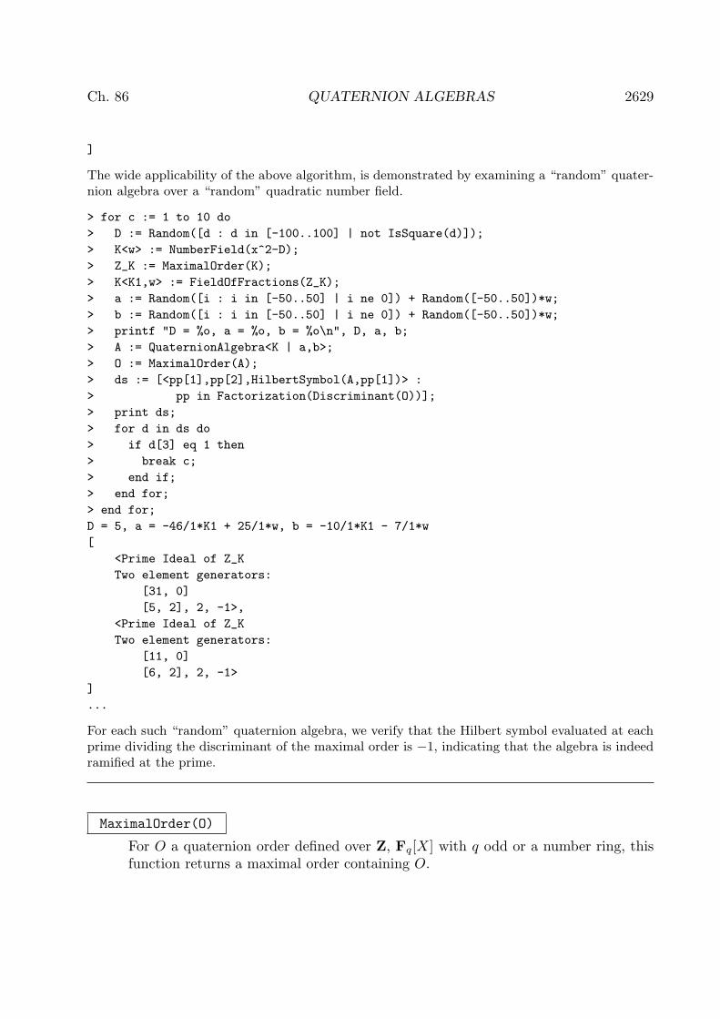
Ch. 86 QUATERNION ALGEBRAS 2629
]
The wide applicability of the above algorithm, is demonstrated by examining a “random” quater-nion algebra over a “random” quadratic number field.
> for c := 1 to 10 do
> D := Random([d : d in [-100..100] | not IsSquare(d)]);
> K<w> := NumberField(x^2-D);
> Z_K := MaximalOrder(K);
> K<K1,w> := FieldOfFractions(Z_K);
> a := Random([i : i in [-50..50] | i ne 0]) + Random([-50..50])*w;
> b := Random([i : i in [-50..50] | i ne 0]) + Random([-50..50])*w;
> printf "D = %o, a = %o, b = %o\n", D, a, b;
> A := QuaternionAlgebra<K | a,b>;
> O := MaximalOrder(A);
> ds := [<pp[1],pp[2],HilbertSymbol(A,pp[1])> :
> pp in Factorization(Discriminant(O))];
> print ds;
> for d in ds do
> if d[3] eq 1 then
> break c;
> end if;
> end for;
> end for;
D = 5, a = -46/1*K1 + 25/1*w, b = -10/1*K1 - 7/1*w
[
<Prime Ideal of Z_K
Two element generators:
[31, 0]
[5, 2], 2, -1>,
<Prime Ideal of Z_K
Two element generators:
[11, 0]
[6, 2], 2, -1>
]
...
For each such “random” quaternion algebra, we verify that the Hilbert symbol evaluated at eachprime dividing the discriminant of the maximal order is −1, indicating that the algebra is indeedramified at the prime.
MaximalOrder(O)
For O a quaternion order defined over Z, Fq[X] with q odd or a number ring, thisfunction returns a maximal order containing O.

2630 ALGEBRAS Part XII
pMaximalOrder(O, p)
For O a quaternion order defined over Z, Fq[X] with q odd or a number ring and aprime (ideal) p, this function returns a p-maximal order O′ containing the order O.The p-adic valuation of the discriminant of O′ (which is either 0 or 1) is returnedas a second return value.
TameOrder(A)
Given a quaternion algebra A, this function returns an order O having the propertythat the odd reduced discriminant of O is squarefree. The algebra A must be definedover a number field or field of fractions of a number ring. The algorithm ignoreseven primes and does not test the remaining odd primes for maximality.
86.3.3 Creation of Orders with given DiscriminantThe following two functions together with the maximal order algorithms of the previoussubsection allow the construction of arbitrary Eichler orders.
Order(O, N)
Given an order O in a quaternion algebra A over the rationals or Fq(x) with q odd,and some element N in the base ring of O, this function returns a suborder O′ of Ohaving index N . Currently, N and the level of O must be coprime and N must havevaluation at most 1 at each ramified prime of A. The order O′ is locally Eichler atall prime divisors of N that are not ramified in A. In particular, if O is Eichler andN is coprime to the discriminant of A, so is O′.
Order(O, N)
Given a maximal quaternion order O over a number ring, this function returns anEichler order of level N inside O.
GorensteinClosure(O)
Given a quaternion order O over the integers, Fq[x] with q odd or a number ring,this function returns the smallest Gorenstein order containing O.
Example H86E7
First we construct a quaternion algebra A over F5(x) ramified at x2 +x+1, then a maximal orderM in A and finally an Eichler O order of discriminant (x2 + x + 1)(x3 + x + 1)5.
> P<x> := PolynomialRing(GF(5));
> A := QuaternionAlgebra(x^2+x+1);
> M := MaximalOrder(A);
> O := Order(M, (x^3+x+1)^5);
> FactoredDiscriminant(O);
[
<x^2 + x + 1, 1>,
<x^3 + x + 1, 5>
]

Ch. 86 QUATERNION ALGEBRAS 2631
86.3.4 Creation of Orders with given Discriminant over the Integers
When constructing quaternion orders over the integers, several shortcuts are available.
QuaternionOrder(A, M)
Given a quaternion algebra A and a positive integer M , this function returns anorder of index M in a maximal order of the quaternion algebra A defined over Q.The second argument M can have at most valuation 1 at any ramified prime of A.
QuaternionOrder(N)
QuaternionOrder(N, M)
Given positive integers N and M , this function returns an order of index M ina maximal order of the rational quaternion algebra A of discriminant N . Thediscriminant N must be a product of an odd number of distinct primes, and theargument M can be at most of valuation 1 at any prime dividing N . If M is omitted,the integer M defaults to 1, i.e., the function will return a maximal order.
QuaternionOrder(D1, D2, T)
This intrinsic constructs the quaternion order Z〈x, y〉, where Z[x] and Z[y] arequadratic subrings of discriminant D1 and D2, respectively, and Z[xy − yx] is aquadratic subring of discriminant D1D2 − T 2.
Note that the container algebra of such a quaternion order is not usually instandard form (see the example below).
Example H86E8
The above constructors permit the construction of Eichler orders over Z, if the discriminant Nand the index M are coprime. More generally they allow the construction of an order whose indexin an Eichler order divides the discriminant.
> A := QuaternionOrder(103,2);
> Discriminant(A);
206
> Factorization($1);
[ <2, 1>, <103, 1> ]
> _<x> := PolynomialRing(Rationals());
> [MinimalPolynomial(A.i) : i in [1..4]];
[
x - 1,
x^2 + 1,
x^2 - x + 52,
x^2 + 104
]
The constructor QuaternionOrder(D1, D2, T) may return an order whose container algebra isnot in standard form.
> A := QuaternionOrder(-4, 5, 2);

2632 ALGEBRAS Part XII
> B := Algebra(A);
> B.1 * B.2 eq - B.2 * B.1;
false
86.4 Elements of Quaternion Algebras
For more information about elements of orders of associative algebras, see Section 81.4.
86.4.1 Creation of Elements
A ! 0
Zero(A)
The zero element of the quaternion algebra A.
A ! 1
One(A)
The identity element of the quaternion algebra A.
A . i
Name(A, i)
Given a quaternion algebra A and an integer 1 ≤ i ≤ 3, returns the ith generatorof A as an algebra over the base ring. Note that the element 1 is always the firstelement of a basis, and is never returned as a generating element.
A ! x
Return an element of the quaternion algebra A described by x, where x may bean algebra element, a module element, a sequence, an element of an order of anassociative algebra or be coercible into the coefficient ring of A.
86.4.2 Arithmetic of Elements
x + y
The sum of x and y.
x - y
The difference of x and y.
x * y
The product of x and y.
x / y
The quotient of x by the unit y in the quaternion algebra.

Ch. 86 QUATERNION ALGEBRAS 2633
x eq y
Returns true if the elements x and y are equal; otherwise false.
x ne y
Returns true if and only if the elements x and y are not equal.
x in A
Returns true if and only if x is in the algebra A.
x notin A
Returns true if and only if x is not in the algebra A.
Conjugate(x)
The conjugate x of the element x of a quaternion algebra, defined so that the reducedtrace and reduced norm are x+ x and xx, respectively.
ElementToSequence(x)
Eltseq(x)
Coordinates(x)
Given an element x of a quaternion algebra or order, this function returns thesequence of coordinates of x in terms of the basis of its parent.
Norm(x)
The reduced norm N(x) of the element x of a quaternion algebra, defined so thatthe characteristic polynomial for x is x2 − Tr(x)x + N(x) = 0, where Tr(x) is thereduced trace.
Trace(x)
The reduced trace Tr(x) of the element x of a quaternion algebra, defined so thatthe characteristic polynomial for x is x2 − Tr(x)x + N(x) = 0, where N(x) is thereduced norm.
CharacteristicPolynomial(x)
The characteristic polynomial of degree 2 for the element x of a quaternion algebraover the base ring of its parent.
MinimalPolynomial(x)
The minimal polynomial of degree 1 or 2 for the element x of a quaternion algebraover the base ring of its parent.

2634 ALGEBRAS Part XII
Example H86E9
We demonstrate the relation between characteristic polynomial, and reduced trace and norm inthe following example.
> A := QuaternionAlgebra< RationalField() | -17, -271 >;
> x := A![1,-2,3,0];
> Trace(x);
2
> Norm(x);
2508
> x^2 - Trace(x)*x + Norm(x);
0
Note that trace and norm of an element x of any algebra can be defined as the trace and normof the linear operator corresponding to right-multiplication by x. The reduced trace and norm ina quaternion algebra A are taken instead to be the corresponding trace and determinant in anytwo-dimensional matrix representation of A, or equivalently, the sum and product of an elementwith its conjugate. The definition of norm and trace used for a general algebra can be realised ina quaternion algebra by the following code.
> P<X> := PolynomialRing(RationalField());
> M := RepresentationMatrix(x, A);
> M;
[ 1 -2 3 0]
[ 34 1 0 3]
[-813 0 1 2]
[ 0 -813 -34 1]
> Trace(M);
4
> Factorization(CharacteristicPolynomial(M));
[
<X^2 - 2*X + 2508, 2>
]
The general definition of trace (for the algebra) is twice the reduced trace, and the general defi-nition of norm is the square of the reduced norm.
86.5 Attributes of Quaternion Algebras
BaseField(A)
BaseRing(A)
The base field of the quaternion algebra A.
Basis(A)
The basis of the algebra A.

Ch. 86 QUATERNION ALGEBRAS 2635
RamifiedPrimes(A)
Given a quaternion algebra A over Q or Fq(X) with q odd, this function returnsa list of primes or normalized irreducible polynomials corresponding to the finiteramified places of A.
Example H86E10
The sequence of ramified primes of a quaternion algebra A over Q determines the isomorphismclass of the algebra.
> A := QuaternionAlgebra(-436,-503,22);
> RamifiedPrimes(A);
[ 17 ]
Provided the discriminant is of a size which can be factored, the ramified primes are determinedefficiently using Hilbert symbols.
RamifiedPlaces(A)
FactoredDiscriminant(A)
Given a quaternion algebra A over Q or Fq(X) with q odd or a number field, thisfunction returns the finite as well as infinite places where A is ramified.
Note: The first return value of these functions is always a list of ideals, even ifthe algebra is given over Q or Fq(X).
Example H86E11
This example shows the (minor) difference between RamifiedPrimes and RamifiedPlaces.
> F<x> := RationalFunctionField( GF(5) );
> A := QuaternionAlgebra< F | 2, x >;
> R<x>:= Integers(F);
> RamifiedPrimes(A);
[ x ]
> RamifiedPlaces(A);
[
Ideal of Univariate Polynomial Ring in x over GF(5) generated by x
]
[ Infinity ]
Discriminant(A)
The reduced discriminant of a quaternion algebra A over Q, Fq(X) with q odd or anumber field. In the first two cases, the functions return the product of the ramifiedprimes. Over number fields, they return the product of the ramified prime ideals aswell as the sequence of ramified infinite places.

2636 ALGEBRAS Part XII
StandardForm(A)
Returns integers a and b in the base field F of the given quaternion algebra A suchthat there exists elements i, j ∈ A where i2 = a, j2 = b, and ji = −ij. The third ob-ject returned is the standard quaternion algebra B = QuaternionAlgebra<F|a,b>,and the fourth object is the homomorphism from A to B.
86.6 Hilbert Symbols and EmbeddingsLet A be a quaternion algebra overQ, Fq(X) (with q odd) or a number field F with definingelements a, b, and let v be a place of F . If v is unramified in A (i.e. A ⊗F Fv
∼= M2(Fv),we define the Hilbert symbol (a, b)v to be 1, and otherwise we define (a, b)v = −1.
HilbertSymbol(a, b, p)
HilbertSymbol(A, p)
Al MonStgElt Default : “NormResidueSymbol”Computes the Hilbert symbol for the quaternion algebra A over F , namely (a, b)p,where a, b ∈ F and p is either a prime (if a, b ∈ Q or Fq(X)) or a prime ideal. Ifa, b ∈ Q, by default table-lookup is used to compute the Hilbert symbol; one canoptionally insist on using the full algorithm by setting the parameter Al to the value"Evaluate".
IsRamified(p, A)
IsUnramified(p, A)
Returns true if and only if the prime or prime ideal p is ramified (unramified) inthe quaternion algebra A.
Example H86E12
We first verify the correctness of all Hilbert symbols over the rationals.
> QQ := Rationals();
> for a,b in [1..8] do
> bl := HilbertSymbol(QQ ! a, QQ ! b,2 : Al := "Evaluate")
> eq NormResidueSymbol(a,b,2);
> print <a,b,bl>;
> if not bl then
> break a;
> end if;
> end for;
<1, 1, true>
<1, 2, true>
<1, 3, true>
...
For a second test, we input a quaternion algebra which is unramified at all finite places.
> P<x> := PolynomialRing(Rationals());
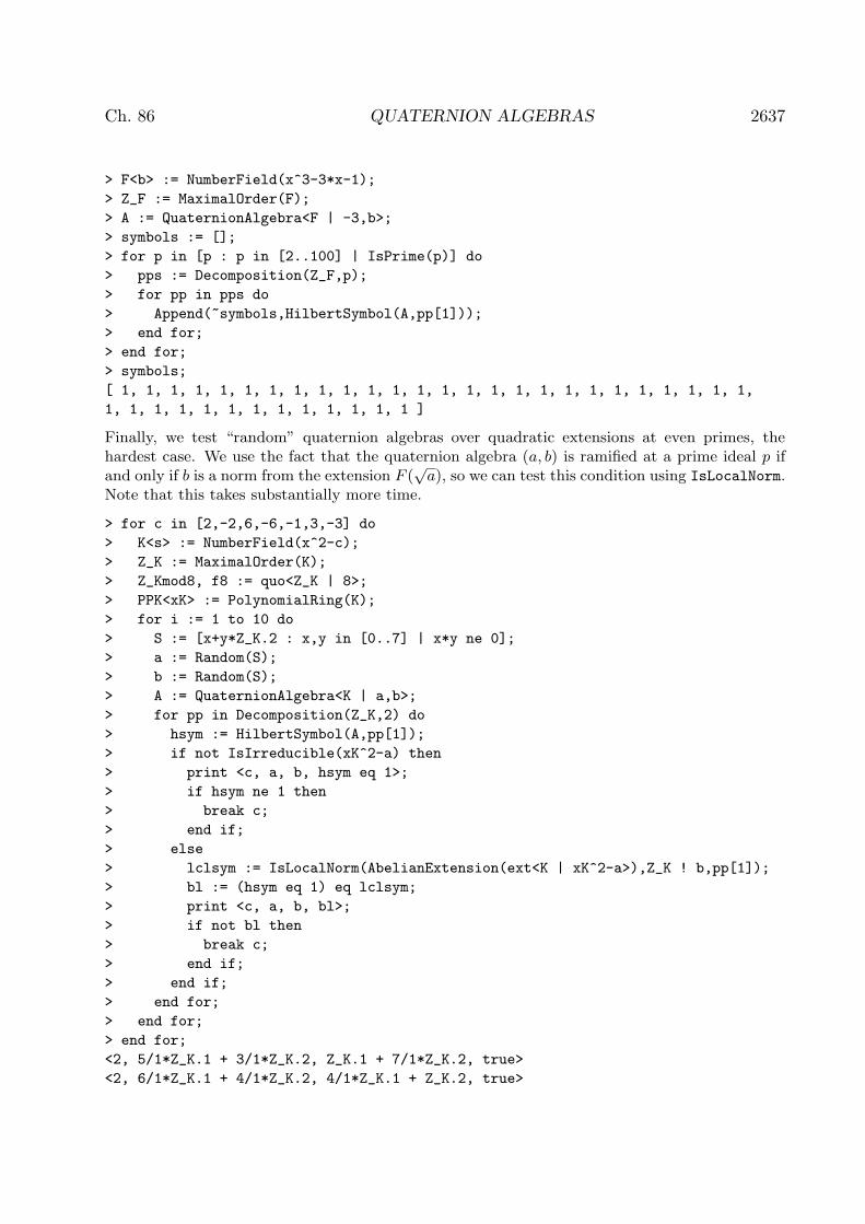
Ch. 86 QUATERNION ALGEBRAS 2637
> F<b> := NumberField(x^3-3*x-1);
> Z_F := MaximalOrder(F);
> A := QuaternionAlgebra<F | -3,b>;
> symbols := [];
> for p in [p : p in [2..100] | IsPrime(p)] do
> pps := Decomposition(Z_F,p);
> for pp in pps do
> Append(~symbols,HilbertSymbol(A,pp[1]));
> end for;
> end for;
> symbols;
[ 1, 1, 1, 1, 1, 1, 1, 1, 1, 1, 1, 1, 1, 1, 1, 1, 1, 1, 1, 1, 1, 1, 1, 1, 1, 1,
1, 1, 1, 1, 1, 1, 1, 1, 1, 1, 1, 1, 1 ]
Finally, we test “random” quaternion algebras over quadratic extensions at even primes, thehardest case. We use the fact that the quaternion algebra (a, b) is ramified at a prime ideal p ifand only if b is a norm from the extension F (
√a), so we can test this condition using IsLocalNorm.
Note that this takes substantially more time.
> for c in [2,-2,6,-6,-1,3,-3] do
> K<s> := NumberField(x^2-c);
> Z_K := MaximalOrder(K);
> Z_Kmod8, f8 := quo<Z_K | 8>;
> PPK<xK> := PolynomialRing(K);
> for i := 1 to 10 do
> S := [x+y*Z_K.2 : x,y in [0..7] | x*y ne 0];
> a := Random(S);
> b := Random(S);
> A := QuaternionAlgebra<K | a,b>;
> for pp in Decomposition(Z_K,2) do
> hsym := HilbertSymbol(A,pp[1]);
> if not IsIrreducible(xK^2-a) then
> print <c, a, b, hsym eq 1>;
> if hsym ne 1 then
> break c;
> end if;
> else
> lclsym := IsLocalNorm(AbelianExtension(ext<K | xK^2-a>),Z_K ! b,pp[1]);
> bl := (hsym eq 1) eq lclsym;
> print <c, a, b, bl>;
> if not bl then
> break c;
> end if;
> end if;
> end for;
> end for;
> end for;
<2, 5/1*Z_K.1 + 3/1*Z_K.2, Z_K.1 + 7/1*Z_K.2, true>
<2, 6/1*Z_K.1 + 4/1*Z_K.2, 4/1*Z_K.1 + Z_K.2, true>

2638 ALGEBRAS Part XII
<2, 7/1*Z_K.1 + Z_K.2, 2/1*Z_K.1 + 2/1*Z_K.2, true>
...
pMatrixRing(A, p)
pMatrixRing(O, p)
Precision RngIntElt Default :
Let A be a quaternion algebra A over a field F where F is the rationals, a numberfield of Fq(x) with q odd. Given A and a prime (ideal) p of the ring of integers Rof F such that p is unramified in A, this function returns the matrix ring over thecompletion Fp of F at p, a map from A→M2(Fp) and the embedding F → Fp.
Given a p-maximal order O in A, the map from A → M2(Fp) induces a mapfrom O → M2(Rp).
IsSplittingField(K, A)
HasEmbedding(K, A)
ComputeEmbedding BoolElt Default : false
Given a quaternion algebra A defined over Q, Fq(X) (with q odd) or a number fieldF and K a quadratic extension of F , the function returns true if and only if thereexists an embedding K → A over F . This is done by comparison of ramified placesin K and A (see [Vig80, Cor. III.3.5]). If no embedding exists, the second returnvalue will be a witness place. If an embedding exists and the optional argumentComputeEmbedding is set to true, the second and third return values contain theresult of a call to Embed as described below.
Embed(K, A)
Al MonStgElt Default : “NormEquation”
Given a quaternion algebra A defined over Q, Fq(X) (with q odd) or a number fieldF and K a quadratic extension of F , returns an embedding K → A over F , givenas an element of A, the image of the primitive generator of K, and the map K → A.
The algorithm by default involves solving a relative norm equation. Alterna-tively, a naive search algorithm may be selected by setting the optional parameterAl:="Search".
If there is no embedding, a runtime error occurs (or the "Search" runs forever).To check whether an embedding exists, use HasEmbedding (see immediately above).

Ch. 86 QUATERNION ALGEBRAS 2639
Embed(Oc, O)
Al MonStgElt Default : “NormEquation”Given a quadratic order Oc with base number ring R and a quaternion order O withbase ring R, the function computes an embedding Oc → O over R. It returns theimage of the second generator Oc.2 of Oc; secondly it returns the embedding mapOc → O.
The algorithm by default involves solving a relative norm equation. Alterna-tively, a naive search algorithm may be selected by setting the optional parameterAl:="Search".
Notes. Let K be the number field containing Oc.(i) Oc.1, Oc.2 are the generators of Oc as a module, and Oc.2 is unrelated to
K.1, where K is the number field containing Oc.(ii) To check whether an embedding of K into the algebra exists, one can use
HasEmbedding(K, Algebra(O) : ComputeEmbedding:=false).
Example H86E13
> F<b> := NumberField(Polynomial([1,-3,0,1]));
> A := QuaternionAlgebra<F | -3, b>;
> K := ext<F | Polynomial([2,-1,1])>;
> mu, iota := Embed(K, A);
> mu;
1/2 + 1/6*(-2*b^2 + 2*b + 7)*i + 1/2*(2*b^2 + b - 6)*j + 1/6*(-2*b^2 - b + 4)*k
> MinimalPolynomial(mu);
$.1^2 - $.1 + 2
> iota(K.1) eq mu;
true
86.7 Predicates on Algebras
A quaternion algebra A over a number field F with [F : Q] = h is definite (or totallydefinite) if F is totally real and A ⊗Q R ∼= Hh, where H is the division ring of realHamiltonians, otherwise A is indefinite.
A quaternion algebra A over Fq(X) is called definite if the place corresponding to thedegree valuation is ramified.
IsDefinite(A)
IsIndefinite(A)
Given a quaternion algebra A over a number field, Q or Fq(X) with q odd, re-turns true if and only if A is a (totally) definite or indefinite quaternion algebra,respectively.

2640 ALGEBRAS Part XII
86.8 Recognition FunctionsA quaternion algebra A over a field K is isomorphic to the matrix ring M2(K) if and only ifthere exists a zerodivisor ε in A. Given such an ε, we can exhibit an explicit isomorphism;otherwise a zerodivisor will be computed first by finding a point on a conic (see [Vig80,Cor. I.2.4]).
Given an associative algebra, we also have an algorithm to recognize if the algebra is aquaternion algebra, and, if so, return an isomorphism to a quaternion algebra in standardform.
IsMatrixRing(A)
Isomorphism BoolElt Default : false
Returns true if and only if the quaternion algebra A with base field F is isomorphicto M2(F ), or equivalently if A has no ramified places. The field F has to be Q,Fq(X) (with q odd) or a number field.
If A is isomorphic to M2(F ) and Isomorphism is set to true, then M2(F ) andan isomorphism A→M2(F ) are also returned.
MatrixRing(A, eps)
MatrixAlgebra(A, eps)
Given a quaternion algebra A and a zerodivisor ε ∈ A, the function returns thematrix algebra M2(F ) and an isomorphism A→M2(F ).
Example H86E14
> A := QuaternionAlgebra<Rationals() | -1, 1>;
> eps := A.3-1;
> MinimalPolynomial(eps), Norm(eps);
x^2 + 2*x
0
Thus, since ε has reduced norm 0, it is a zerodivisor: indeed, ε(ε + 2) = 0.
> M2F, phi := MatrixRing(A,eps);
> [<MinimalPolynomial(A.i), MinimalPolynomial(phi(A.i))> : i in [1..3]];
[
<x^2 + 1, x^2 + 1>,
<x^2 - 1, x^2 - 1>,
<x^2 - 1, x^2 - 1>
]
IsQuaternionAlgebra(B)
Returns true if and only if the associative algebra B is a quaternion algebra; iftrue, it returns the associated quaternion algebra A in standard form and an algebrahomomorphism from B to A. The algorithm used is [Voi05, Algorithm 4.2.9].

Ch. 86 QUATERNION ALGEBRAS 2641
Example H86E15
We create an associative algebra which is known to be a quaternion algebra A and then recoverA (or an isomorphic algebra).
> A := AssociativeAlgebra(QuaternionAlgebra<Rationals() | -1,1>);
> vecs := [&+[Random(10)*A.i : i in [1..4]] : j in [1..4]];
> Mchange := Matrix(Rationals(),4,4,&cat[Eltseq(vecs[i]) : i in [1..4]]);
> Mchange := Mchange^(-1);
> seq := [<i,j,k,((vecs[i]*vecs[j])*Mchange)[k]> : i,j,k in [1..4]];
> A := AssociativeAlgebra<Rationals(),4 | seq>;
> bl, Aquat, phi := IsQuaternionAlgebra(A);
> bl;
true
> Aquat;
Quaternion Algebra with base ring Rational Field
> Aquat.1^2, Aquat.2^2;
25 -3924/25
> phi;
Mapping from: AlgAss: A to AlgQuat: Aquat given by a rule
We now verify the functionality when a zerodivisor is encountered.
> A := Algebra(MatrixAlgebra(Rationals(),2));
> IsQuaternionAlgebra(A);
true Quaternion Algebra with base ring Rational Field
Mapping from: AlgAss: A to Quaternion Algebra with base ring Rational Field
given by a rule
The algebra k < x, y > with x2 = y2 = xy + yx = 0 is not semisimple; the ideal generated by x, yis a nontrivial two-sided ideal. Similarly, a commutative algebra is not a quaternion algebra.
> A := Algebra(FPAlgebra<Rationals(), x,y | x^2, y^2, x*y+y*x>);
> IsQuaternionAlgebra(A);
false
> A := Algebra(FPAlgebra<Rationals(), x | x^4+x^2+1>);
> IsQuaternionAlgebra(A);
false
In characteristic 2, the algorithm also performs correctly, both for an associative but non-quaternion algebra and for the “universal” example of a quaternion algebra.
> A := Algebra(FPAlgebra<GF(2), x,y | x^2, y^2, x*y+y*x+1>);
> IsQuaternionAlgebra(A);
false
> F<a,b,x,y,z,w> := FieldOfFractions(PolynomialRing(GF(2),6));
> M := [[1,0,0,0],[0,1,0,0],[0,0,1,0],[0,0,0,1],
> [0,1,0,0],[a,1,0,0],[0,0,0,1],[0,0,a,1],
> [0,0,1,0],[0,0,1,1],[b,0,0,0],[b,b,0,0],
> [0,0,0,1],[0,0,a,0],[0,b,0,0],[a*b,0,0,0]];
> A<alpha,beta> := AssociativeAlgebra<F,4 | M>;

2642 ALGEBRAS Part XII
> alpha^2+alpha+a;
(0 0 0 0)
> beta^2+b;
(0 0 0 0)
>
> bl, Aquat, phi := IsQuaternionAlgebra(A);
> bl;
true
> Aquat;
Quaternion Algebra with base ring Multivariate rational function field of
rank 6 over GF(2)
> theta := phi(x+y*alpha+z*beta+w*alpha*beta);
> Trace(theta);
y
> Norm(theta);
a*b*w^2 + a*y^2 + b*z^2 + b*z*w + x^2 + x*y
MatrixRepresentation(A)
MatrixRepresentation(R)
Given a quaternion algebra A over Q or a quaternion order R over Z, this functionreturns a 2× 2-matrix representation of A, defined over a quadratic extension.
86.9 Attributes of Orders
For further information about orders of associative algebras, see Section 81.4.For a quaternion order S over Z or Fq[X], Magma additionally defines the following
functions.
Algebra(S)
QuaternionAlgebra(S)
The quaternion algebra for which S is an order.
BasisMatrix(S)
EmbeddingMatrix(S)
Returns the basis matrix of the quaternion order S over Z or Fq[X]. The rows ofthe matrix give the basis elements of S with respect to the basis of the containeralgebra.
Discriminant(S)
Given an order S over Z or Fq[X], this function returns the reduced discriminantof S as a positive integer or a normalized polynomial.

Ch. 86 QUATERNION ALGEBRAS 2643
FactoredDiscriminant(S)
Given a quaternion order S, this function returns the factorisation of the reduceddiscriminant of S (that is, Factorization(Discriminant(S))).
Conductor(S)
Level(S)
Given an order S over Z or Fq[X] in a quaternion algebra A, this function returnsthe reduced index of S in a maximal order of A containing it. Together with thereduced discriminant of the order, this serves to classify the local isomorphism classof an Eichler order.
Normalizer(S)
Let S be an order in a definite quaternion algebra A over a field F where F isthe rationals, Fq(t) or a number field. This function returns a matrix group Gisomorphic to the normalizer of S in A∗ modulo F ∗. A homomorphism from G toA∗ is also returned.
86.10 Predicates of Orders
Let O be a quaternion order with base ring Z, Fq[X] with q odd, or a number ring. ThenMagma can test the following predicates.
IsMaximal(O)
Returns true if and only if the order O is maximal.
IspMaximal(O, p)
Returns true if and only if the order O is maximal at the prime or prime ideal p.
IsEichler(O)
MaximalOrders BoolElt Default : false
Returns true if and only if the order O is Eichler, that is an intersection of two(not necessarily distinct) maximal orders. The function calls the EichlerInvariantintrinsic explained below.
If the optional argument MaximalOrders is set to true, the algorithm also returnstwo maximal orders such that O is their intersection.
IsEichler(O, p)
MaximalOrders BoolElt Default : false
Returns true if and only if the completion of the order O at the prime (ideal) p isEichler.
If the optional argument MaximalOrders is set to true, the algorithm also returnstwo p-maximal orders such that O is their intersection.

2644 ALGEBRAS Part XII
EichlerInvariant(O, p)
Returns the local Eichler invariant of O at some prime (ideal) p which divides thediscriminant of O. Let R be the base ring of O and let J be the Jacobson radical ofthe R/p-algebra O/pO. If J has dimension 3 then the Eichler invariant is defined tobe 0. Otherwise the quotient of O/pO by J is either isomorphic to a direct sum oftwo copies of R/p or a quadratic field extension of R/p. In the first case the Eichlerinvariant is 1, in the latter it is −1.
IsHereditary(O)
Returns true if and only if the order O is a hereditary order in a quaternion algebraA. That is, every lattice in A of full rank such that O is contained in its left order is aprojective left O-module. The hereditary orders are precisely those with squarefreediscriminant.
IsHereditary(O, p)
Returns true if and only if the completion of the order O at the prime (ideal) p ishereditary.
IsGorenstein(O)
Returns true if and only if the order O is a Gorenstein order. That is, the dual ofO with respect to the trace bilinear form is a projective O-module.
IsGorenstein(O, p)
Returns true if and only if the completion of the order O at the prime (ideal) p isGorenstein.
86.11 Operations with Orders
O1 meet O2
This returns the order obtained by intersecting the quaternion orders O1 and O2.
O ^ x
This returns the conjugate of the order O by an element x in the associative algebraA for which O is an order (in other words the order x−1Ox).

Ch. 86 QUATERNION ALGEBRAS 2645
86.12 Ideal Theory of Orders
The right (or left) ideals of an R-order O in a quaternion algebra A defined over a numberfield fall into finitely many isomorphism classes. Already, for the case of number rings, itis a computationally difficult problem to compute the class group, and due to the noncom-mutativity of quaternion algebras, the problem of enumerating ideal classes of quaternionorders is even more difficult because this set does not have the structure of a group.
All orders in this section are required to be Eichler. The reader should recall that thisincludes the maximal orders.
The algorithms underpinning the intrinsics described in this section, in particular, thosefor determining ideal classes, are described in [KV10]. The methods depend on whether Ais definite or indefinite. For a definite algebra, we use a variation of Kneser’s neighbouringmethod together with Eichler’s mass formula (see [Vig80, Chapter 5] and [DG88]) toconstruct sufficient ideals to represent all ideal classes. We then test if two right (or left)ideals I, J are isomorphic (Section 86.14.3).
For an indefinite quaternion algebra, we use a theorem of Eichler [Rei03, Th. 35.14]which states that the reduced norm gives rise to an bijection of sets between the classgroups of the order and the number ring. (Over Z or Fq[X], therefore, every ideal of anindefinite quaternion order is principal.) We may compute representative ideals I of Owhose reduced norm is in a specified ideal class. We then reduce the problem of testingfor an isomorphism I ∼= J between two ideals to the similar problem over R. Here, theproblem of explicitly computing such an isomorphism is much less difficult, as an order(or ideal) will have infinitely many elements of bounded norm, and in most cases a searchamongst reduced bases will find a desired element.
Ideals of quaternion orders belong to the types AlgQuatOrdIdl and AlgAssVOrdIdlaccording as to whether the order O is defined over Z or Fq[X] (both of type AlgQuatOrd)or over a number ring (of type AlgAssVOrd). For more on the constructions and functionsfor ideals of the latter type, see Section 81.4.
86.12.1 Creation and Access Functions
LeftIdeal(S, X)
lideal< S | X >
RightIdeal(S, X)
rideal< S | X >
ideal< S | X >
These intrinsics construct a left, right or two-sided ideal of the order S generated bythe sequence X, which should contain elements that are coercible into the algebraof S.
In the case of the constructors lideal< | > and rideal< | >, the right handside may also be a matrix or pseudo-matrix giving the basis of the ideal with respectto the basis of S.
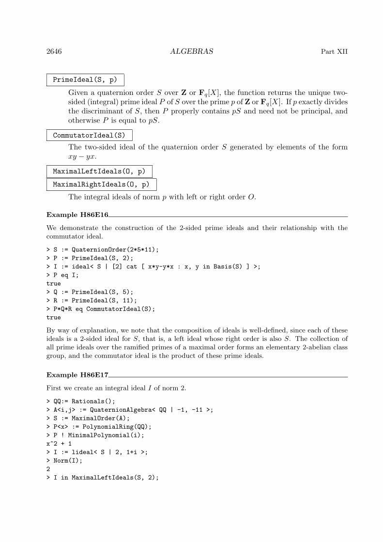
2646 ALGEBRAS Part XII
PrimeIdeal(S, p)
Given a quaternion order S over Z or Fq[X], the function returns the unique two-sided (integral) prime ideal P of S over the prime p of Z or Fq[X]. If p exactly dividesthe discriminant of S, then P properly contains pS and need not be principal, andotherwise P is equal to pS.
CommutatorIdeal(S)
The two-sided ideal of the quaternion order S generated by elements of the formxy − yx.
MaximalLeftIdeals(O, p)
MaximalRightIdeals(O, p)
The integral ideals of norm p with left or right order O.
Example H86E16
We demonstrate the construction of the 2-sided prime ideals and their relationship with thecommutator ideal.
> S := QuaternionOrder(2*5*11);
> P := PrimeIdeal(S, 2);
> I := ideal< S | [2] cat [ x*y-y*x : x, y in Basis(S) ] >;
> P eq I;
true
> Q := PrimeIdeal(S, 5);
> R := PrimeIdeal(S, 11);
> P*Q*R eq CommutatorIdeal(S);
true
By way of explanation, we note that the composition of ideals is well-defined, since each of theseideals is a 2-sided ideal for S, that is, a left ideal whose right order is also S. The collection ofall prime ideals over the ramified primes of a maximal order forms an elementary 2-abelian classgroup, and the commutator ideal is the product of these prime ideals.
Example H86E17
First we create an integral ideal I of norm 2.
> QQ:= Rationals();
> A<i,j> := QuaternionAlgebra< QQ | -1, -11 >;
> S := MaximalOrder(A);
> P<x> := PolynomialRing(QQ);
> P ! MinimalPolynomial(i);
x^2 + 1
> I := lideal< S | 2, 1+i >;
> Norm(I);
2
> I in MaximalLeftIdeals(S, 2);

Ch. 86 QUATERNION ALGEBRAS 2647
true
We now examine the basis of the ideal I.
> Basis(I);
[ 2, 1 + i, i + k, 3/2 + 1/2*i + 1/2*j + 1/2*k ]
> [ Eltseq(x) : x in Basis(I) ];
[
[ 2, 0, 0, 0 ],
[ 1, 1, 0, 0 ],
[ 0, 1, 0, 1 ],
[ 3/2, 1/2, 1/2, 1/2 ]
]
> BasisMatrix(I, A);
[ 2 0 0 0]
[ 1 1 0 0]
[ 0 1 0 1]
[3/2 1/2 1/2 1/2]
If the ideal I is printed, the rational coordinates with respect to the basis of the quaternion orderS will be shown, We can get this base change matrix if we call BasisMatrix with no additionalparameters.
> I;
Left Ideal with basis Pseudo-matrix over Integer Ring
[2 0 0 0]
[1 1 0 0]
[0 0 2 0]
[1 0 1 1]
> BasisMatrix(I);
[2 0 0 0]
[1 1 0 0]
[0 0 2 0]
[1 0 1 1]
LeftOrder(I)
Given an ideal I of a quaternion order defined over Z, Fq[X] or a number ring,this function returns the left order of I, defined as the ring of all elements of thequaternion algebra of I mapping I to itself under left multiplication.
RightOrder(I)
Given an ideal I of a quaternion order defined over Z, Fq[X] or a number ring,this function returns the right order of I, defined as the ring of all elements of thequaternion algebra of I mapping I to itself under right multiplication.

2648 ALGEBRAS Part XII
Example H86E18
> K := NumberField(Polynomial([5,0,1]));
> K;
Number Field with defining polynomial $.1^2 + 5 over the Rational Field
> A := QuaternionAlgebra<K | 3, K.1>;
> O := MaximalOrder(A);
> I := lideal<O | O.2, Norm(O.2)>;
> Norm(I);
Principal Ideal
Generator:
2/1*$.1
> LeftOrder(I) eq O;
true
> RightOrder(I) eq O;
true
86.12.2 Enumeration of Ideal ClassesThe tools provided for calculating ideal classes in the case of a maximal or, more generally,an Eichler order S in a quaternion algebra over Q, Fq(X) (with q odd) or a number fieldare described in this section.
Mass(S)
Given a definite order S of level N over R, this function returns the mass
∑
i
hi/[S∗i : R∗]
where S1, . . . , St represent the conjugacy classes of Eichler orders of level N and hi
denotes the number of two-sided ideal classes of Si.
LeftIdealClasses(S)
RightIdealClasses(S)
Support [RngOrdIdl] Default :
These intrinsics find representatives for the left or right locally free ideal classes ofS, where S is an order in a quaternion algebra A defined over Q, Fq(X) (with qodd) or a number field. The algorithms are guaranteed to work correctly only whenS is a maximal order or an Eichler order.
For definite algebras, the support of the returned ideals may be specified usingparameter Support; this should be a sequence of primes or prime ideals in the basering which generate the narrow class group and which do not ramify in A. In thiscase, the routine will find ideal class representatives whose norms are divisible onlyby primes in the specified support. The algorithm usually runs faster if the support

Ch. 86 QUATERNION ALGEBRAS 2649
is either not specified or if the support includes the prime divisors of the discriminantof S.
For indefinite algebras, the representatives are obtained from a ray class groupof the base field.
TwoSidedIdealClasses(S)
Support [RngOrdIdl] Default :
Given an order S in a quaternion algebra, this function returns a sequence containingrepresentatives for the two-sided locally free ideal classes of S. The algorithm is onlyguaranteed to work when S is a maximal order or an Eichler order.
If the optional argument Support is specified, Magma tries to construct rep-resentatives that have norm divisible by primes or prime ideals in the specifiedsupport. If this is not possible, the set specified using parameter Support will beenlarged by the prime divisors of the discriminant of S. If this enlarged set is stillnot large enough (which can only happen if the set does not generate the class ofgroup of the base ring of S) an error will be raised.
TwoSidedIdealClassGroup(S : Support)
Support [RngOrdIdl] Default :
Given an order S in a quaternion algebra, this returns the two-sided ideal class groupof S as an abstract abelian group, together with a map from the group to the setof two-sided ideal classes of S. Inverses with respect to this map can be calculatedin a very efficient way and thus may be used to compute discrete logarithms. Thealgorithm is only guaranteed to work when S is a maximal order or an Eichler order.
The optional parameter Support may be used to specify a support: this shouldbe a sequence of primes or prime ideals in the base ring which generate the narrowclass group and which do not ramify in the parent algebra.
ConjugacyClasses(S)
Given a maximal order (or an Eichler order S of level N) in a quaternion algebraA, this function returns representatives for the conjugacy classes of maximal orders(or orders of level N) in A.
For definite algebras, the algorithm involves computing the right ideal classes (infact, the two problems are computationally equivalent in practice).
Example H86E19
In the following example we construct a maximal order in the quaternion algebra ramified at 37,and enumerate its left ideal classes.
> S := QuaternionOrder(37);
> ideals := LeftIdealClasses(S);
> [ Basis(I) : I in ideals ];
[
[ 1, i, j, k ],

2650 ALGEBRAS Part XII
[ 2, 2*i, 1 + i + j, i + k ],
[ 2, 2*i, i + j, k ]
]
We now compute the right orders of the two nontrivial left ideal classes.
> _, I, J := Explode(ideals);
> R1 := RightOrder(I);
> R2 := RightOrder(J);
> IsIsomorphic(R1,R2);
true
Although the ideals I and J are non-isomorphic left ideals over S, they have isomorphic rightorders. In the example following the next section we explore this phenomenon further.
Example H86E20
In this example, we enumerate ideal classes for a definite quaternion algebra (over a totally realfield).
> P<x> := PolynomialRing(Rationals());
> F<b> := NumberField(x^3-3*x-1);
> Z_F := MaximalOrder(F);
> Foo := InfinitePlaces(F);
> pp := Decomposition(Z_F, 17)[1][1];
> A := QuaternionAlgebra(pp, Foo);
> O := MaximalOrder(A);
> time Rideals := RightIdealClasses(O);
Time: 0.870
> #Rideals;
2
Example H86E21
In this example the classgroup of the base field is not trivial and there are some ramified primeideals in the algebra. Hence we expect nontrival two-sided ideal classes.
> K:= QuadraticField(401);
> A:= QuaternionAlgebra< K | -1, -1>;
> RamifiedPlaces(A);
[
Prime Ideal
Two element generators:
2
$.2 + 1,
Prime Ideal
Two element generators:
2
$.2 + 2
]

Ch. 86 QUATERNION ALGEBRAS 2651
[ 1st place at infinity, 2nd place at infinity ]
> M:= MaximalOrder(A);
> #TwoSidedIdealClasses(M);
10
> time #RightIdealClasses(M);
140
Time: 6.470
86.12.3 Operations on IdealsIn addition to operations on ideals of orders over more general rings (see Section 81.4), thefollowing operations are defined for ideals of quaternion orders over Z, Fq[X] and numberrings.
I * J
The composite of I and J , where the right order of I equals the left order of J .
I meet J
Given ideals or orders I and J , this function returns the intersection I ∩ J .
Conjugate(I)
Given an ideal I (of a quaternion algebra), this function returns the conjugate ideal.
Norm(I)
Given an ideal I over Z, this function returns the reduced norm of the ideal, definedas the positive generator of the image of the reduced norm map in Q.
Given an ideal I over Fq[X], this function returns the reduced norm of the ideal,defined as the normalized generator of the image of the reduced norm map in Fq(X).
Given an ideal I over a commutative order, this function returns the reducednorm of I as a fractional ideal of the order.
Factorization(I)
Given a two-sided ideal I of an hereditary order O, this function returns the uniquefactorization of I into two-sided O-ideals. The result is a sequence of tuples. Thefirst entry of each tuple is a two-sided ideal of O, the second is its exponent. (If thebase ring of I is Fq[X], then q is currently required to be odd.)

2652 ALGEBRAS Part XII
86.13 Norm Spaces and Basis Reduction
For definite quaternion orders or ideals one can compute reduced bases and Gram matrices.If the base ring of the order or ideal is Z or Fq[X] with q odd, the Gram matrices can
be made unique up to isomorphism. In fact, in these cases, the isomorphism testing ofideals and orders is based on this reduction.
NormSpace(A)
Given a quaternion algebra A over any field F not of characteristic 2, this functionreturns the underlying F -space with inner product the norm form. A map from Ainto the structure is returned as second value.
NormSpace(S)
Given a quaternion order S over Z or Fq[X] (with q odd), this function returns theunderlying module over its base ring, with inner product respect to the norm. Amap from O into the structure is returned as second value.
GramMatrix(S)
GramMatrix(I)
The Gram matrix of the quaternion order S or ideal I over Z or Fq[X] with respectto the norm on the basis for S.
ReducedGramMatrix(S)
Given an order or ideal S over Z in a definite quaternion algebra, this functionreturns the Gram matrix G of the corresponding lattice.
The quaternion ideal machinery makes use of a Minkowski basis reduction algo-rithm which returns a unique normalized reduced Gram matrix G for any definitequaternion ideal. This forms the core of the isomorphism testing for quaternionideals.
ReducedBasis(S)
Given an order or ideal S over Z in a definite quaternion algebra, this functionreturns some basis B of S the Gram matrix G of the corresponding lattice associatedwith S. Note that while there exists a unique Minkowski-reduced Gram matrix G,the basis B is not unique.
Example H86E22
Recall that Minkowski basis reduction is used which returns a unique normalized reduced Grammatrix G for any definite quaternion ideal. This forms the core of the isomorphism testing forquaternion ideals. We illustrate this by applying it to representatives of the set of left ideal classesof an order.
> A := QuaternionOrder(19,2);
> ideals := LeftIdealClasses(A);
> #ideals;
5

Ch. 86 QUATERNION ALGEBRAS 2653
> [ (1/Norm(I))*ReducedGramMatrix(I) : I in ideals ];
[
[ 2 0 1 1]
[ 0 2 1 1]
[ 1 1 20 1]
[ 1 1 1 20],
[6 0 1 3]
[0 6 3 1]
[1 3 8 1]
[3 1 1 8],
[6 0 1 3]
[0 6 3 1]
[1 3 8 1]
[3 1 1 8],
[ 4 0 1 -1]
[ 0 4 1 1]
[ 1 1 10 0]
[-1 1 0 10],
[ 4 0 1 -1]
[ 0 4 1 1]
[ 1 1 10 0]
[-1 1 0 10]
]
ReducedGramMatrix(S)
ReducedBasis(S)
Canonical BoolElt Default : false
Given an order or ideal S over Fq[X] in a quaternion algebra A, this function returnsa Gram matrix and/or a basis of S whose Gram matrix is in dominant diagonal form(see the function DominantDiagonalForm in Section 31.2.1). The Gram matrix willnot be unique unless A is definite and Canonical is set to true.
ReducedBasis(O)
ReducedBasis(I)
Returns a “reduced” basis for the order O or the ideal I over some number ring.If O or I arise from a definite quaternion algebra, then this basis is LLL-reducedwith respect to the norm form; otherwise, the basis is reduced with respect to aMinkowski-like embedding (see [KV10, Section 4]).

2654 ALGEBRAS Part XII
OptimizedRepresentation(O)
OptimisedRepresentation(O)
Given an order O contained in a quaternion algebra A over Q or a number field F ,this function returns a new quaternion algebra A′ such that A′ = ((a, b)/F ) wherea and b are small (with respect to O), and, as second return value, an isomorphismA→ A′.
OptimizedRepresentation(A)
OptimisedRepresentation(A)
Given a quaternion algebra A over Q or a number field F , this function returns anew quaternion algebra A′ such that A′ = ((a, b)/F ) where a and b are small. Anisomorphism A→ A′ is returned as second value.
Enumerate(O, A, B)
The sequence of all elements x (up to sign) in the definite quaternion order O orideal I over Z such that the reduced norm of x lies in the interval [A, . . . B] or[0, . . . B], respectively.
Enumerate(O, A, B)
Enumerate(O, B)
The sequence of elements x (up to sign) in the definite quaternion order O or ideal Iover a number ring such that the absolute trace of the norm of x lies in the interval[A, . . . B] or [0, . . . B], respectively.
86.14 Isomorphisms
86.14.1 Isomorphisms of AlgebrasTwo quaternion algebras A,B over a common field F are isomorphic algebras if and onlyif they share the same ramified places. Finding an explicit isomorphism is much harder.Currently Magma embeds the first standard generator of A into B and then finds anotherelement perpendicular to that image having the correct minimal polynomial. In particular,this requires the construction of two points on a conic (or equivalently, the solution of twonorm equations) over quadratic extensions of F .
IsIsomorphic(A, B)
Isomorphism BoolElt Default : false
Given two quaternion algebras A,B over Q, Fq(X) with q odd or a number field,this function returns true if and only if they are isomorphic.
If the algebras are isomorphic and Isomorphism is set to true, an isomorphismA→ B is also returned.
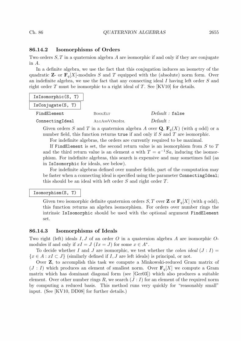
Ch. 86 QUATERNION ALGEBRAS 2655
86.14.2 Isomorphisms of OrdersTwo orders S, T in a quaternion algebra A are isomorphic if and only if they are conjugatein A.
In a definite algebra, we use the fact that this conjugation induces an isometry of thequadratic Z- or Fq[X]-modules S and T equipped with the (absolute) norm form. Overan indefinite algebra, we use the fact that any connecting ideal I having left order S andright order T must be isomorphic to a right ideal of T . See [KV10] for details.
IsIsomorphic(S, T)
IsConjugate(S, T)
FindElement BoolElt Default : false
ConnectingIdeal AlgAssVOrdIdl Default :
Given orders S and T in a quaternion algebra A over Q, Fq(X) (with q odd) or anumber field, this function returns true if and only if S and T are isomorphic.
For indefinite algebras, the orders are currently required to be maximal.If FindElement is set, the second return value is an isomorphism from S to T
and the third return value is an element a with T = a−1Sa, inducing the isomor-phism. For indefinite algebras, this search is expensive and may sometimes fail (asin IsIsomorphic for ideals, see below).
For indefinite algebras defined over number fields, part of the computation maybe faster when a connecting ideal is specified using the parameter ConnectingIdeal;this should be an ideal with left order S and right order T .
Isomorphism(S, T)
Given two isomorphic definite quaternion orders S, T over Z or Fq[X] (with q odd),this function returns an algebra isomorphism. For orders over number rings theintrinsic IsIsomorphic should be used with the optional argument FindElementset.
86.14.3 Isomorphisms of IdealsTwo right (left) ideals I, J of an order O in a quaternion algebra A are isomorphic O-modules if and only if xI = J (Ix = J) for some x ∈ A∗.
To decide whether I and J are isomorphic, we test whether the colon ideal (J : I) =x ∈ A : xI ⊂ J (similarly defined if I, J are left ideals) is principal, or not.
Over Z, to accomplish this task we compute a Minkowski-reduced Gram matrix of(J : I) which produces an element of smallest norm. Over Fq[X] we compute a Grammatrix which has dominant diagonal form (see [Ger03]) which also produces a suitableelement. Over other number rings R, we search (J : I) for an element of the required normby computing a reduced basis. This method runs very quickly for “reasonably small”input. (See [KV10, DD08] for further details.)

2656 ALGEBRAS Part XII
IsIsomorphic(I, J)
Given ideals I and J of the same order O in a quaternion algebra A over Q, Fq(X)(with q odd) or a number field, this function returns true if and only if the quater-nion ideals I and J are isomorphic (left or right) O-ideals. If I and J are isomorphic,there exists some x ∈ A such that xI = J (in the case of right O-ideals) or Ix = J(for left ideals). For definite algebras, such an element x is always returned. Forindefinite algebras over Z or a number ring, a search for such an element is made,and if one is found then it is returned.
IsPrincipal(I)
Given a left (or right) ideal I over Z,Fq[X] or a number ring, this function returnstrue if and only if I is a principal ideal; if so, a generator is returned as the secondvalue.
IsLeftIsomorphic(I, J)
IsRightIsomorphic(I, J)
Given two definite ideals over Z or Fq[X] (with q odd) with the same left (or right)order S, this function returns true if and only if they are isomorphic as S-modules.The isomorphism and the transforming scalar in the quaternion algebra are returnedas second and third values if true.
IsLeftIsomorphic(I, J)
IsRightIsomorphic(I, J)
Given two left (or right) ideals I and J over a number ring, with the same left orderO, this function returns true if and only if they are isomorphic as O-modules. Theisomorphism is given by multiplication as a second return value.
LeftIsomorphism(I, J)
Given two isomorphic left ideals over a definite order S over Z or Fq[X], this func-tion returns the S-module isomorphism between them, followed by the quaternionalgebra element which defines the isomorphism by right-multiplication.
RightIsomorphism(I, J)
Given two isomorphic right ideals over a definite order S over Z or Fq[X], this func-tion returns the S-module isomorphism between them, followed by the quaternionalgebra element which defines the isomorphism by left-multiplication.

Ch. 86 QUATERNION ALGEBRAS 2657
86.14.4 Examples
Example H86E23
In this example, we create two quaternion algebras over F7, show that they are isomorphic andfind an isomorphism between them.
> F<x> := RationalFunctionField( GF(7) );
> Q1 := QuaternionAlgebra< F | (x^2+x-1)*(x+1), x >;
> a := x^3 + x^2 + 3;
> b := x^13 + 4*x^11 + 2*x^10 + x^9 + 6*x^8 + 4*x^5 + 3*x^4 + x;
> Q2:= QuaternionAlgebra< F | a, b >;
> ok, phi:= IsIsomorphic(Q1, Q2 : Isomorphism);
> ok;
true
> forall <x,y> : x,y in Basis(Q1) | phi(x*y) eq phi(x)*phi(y) ;
true
Example H86E24
In this example, we create two ideals, show that they have isomorphic right orders, and thenexplicitly exhibit the isomorphism.
> A := QuaternionAlgebra(37);
> S := MaximalOrder(A);
> ideals := LeftIdealClasses(S);
> _, I, J := Explode(ideals);
> R := RightOrder(I);
> Q := RightOrder(J);
> IsIsomorphic(R,Q);
true
> // Get the x which conjugates R to Q:
> _, pi := Isomorphism(R,Q);
> Norm(pi);
37
> J := lideal< S | [ x*pi : x in Basis(J) ] >;
> RightOrder(J) eq R;
true
Example H86E25
We construct two non-isomorphic left ideals with the same left and right orders, then investigatetheir isomorphisms as right ideals.
> S := QuaternionOrder(37);
> ideals := LeftIdealClasses(S);
> _, I, J := Explode(ideals);
> R := RightOrder(I);
> _, pi := Isomorphism(R,RightOrder(J));

2658 ALGEBRAS Part XII
> J := lideal< S | [ x*pi : x in Basis(J) ] >;
> IsLeftIsomorphic(I,J);
false
> IsRightIsomorphic(I,J);
true Mapping from: AlgQuatOrd: I to AlgQuatOrd: J given by a rule [no inverse]
1 + i - 2*k
> h, x := RightIsomorphism(I,J);
> y := [1,2,-1,3];
> y := &+[y[i]*b[i] : i in [1 .. 4]] where b is Basis(I);
> h(y);
[-73 15 31 4]
> x*y;
-73 + 15*i + 31*j + 4*k
The existence of an isomorphism as a right ideal is due to the fact that the two-sided ideals of Rdo not have non-isomorphic counterparts in S.
> TwoSidedIdealClasses(R);
[ Ideal with basis Pseudo-matrix over Integer Ring
1 * [1 0 0 0]
[0 1 0 0]
[0 0 1 0]
[0 0 0 1]
, Ideal with basis Pseudo-matrix over Integer Ring
1 * [37 0 32 18]
[ 0 37 10 2]
[ 0 0 1 0]
[ 0 0 0 1]
]
> TwoSidedIdealClasses(S);
[ Ideal with basis Pseudo-matrix over Integer Ring
1 * [1 0 0 0]
[0 1 0 0]
[0 0 1 0]
[0 0 0 1]
]
Thus while Conjugate(I)*J is in the non-principal R-ideal class, the ideal I*Conjugate(J) rep-resents the unique principal ideal class of S.
Example H86E26
We exhibit isomorphism testing for ideals of orders over number rings.
> P<x> := PolynomialRing(Rationals());
> F<b> := NumberField(x^3-3*x-1);
> Z_F := MaximalOrder(F);
> F := FieldOfFractions(Z_F);
> A<alpha,beta,alphabeta> := QuaternionAlgebra<F | -3, b>;
> O := Order([alpha,beta,alphabeta]);

Ch. 86 QUATERNION ALGEBRAS 2659
> O;
Order of Quaternion Algebra with base ring F
with coefficient ring Maximal Equation Order with defining polynomial x^3 - 3*x
- 1 over its ground order
> I := ideal<O | 2>;
> I eq (I + ideal<O | 2>);
true
> I eq (I + ideal<O | 3>);
false
>
> Foo := InfinitePlaces(F);
> A := QuaternionAlgebra(ideal<Z_F | 2*3*5>, Foo);
> IsDefinite(A);
true
> O := MaximalOrder(A);
> I := rideal<O | Norm(O.2), O.2>;
> J := rideal<O | Norm(O.3), O.3>;
> IsIsomorphic(I, J);
true (F.2 + F.3) + (27/9190*F.1 - 143/9190*F.2 - 73/9190*F.3)*i +
(-251/27570*F.1 + 7/2757*F.2 + 10/2757*F.3)*k
86.15 Units and Unit Groups
Let S be a definite quaternion order over Z, Fq[X] with q odd, or a number ring. In thefirst two cases, the unit group of S is finite and can be read off any reduced Gram matrixof S. If the base ring of S is some number ring R, then an explicit description of the finitequotient S∗/R∗ is given in [Vig76].
NormOneGroup(S)
ModScalars BoolElt Default : false
Returns a group G isomorphic to the group S1 of elements in S with reduced norm1 (unless ModScalars is set, in which case G is isomorphic to S1 modulo ±1).
The second object returned is a map from G to S expressing the isomorphism.
Units(S)
This intrinsic computes the set of units S∗ for the definite order S. When the basering of S is Z or Fq[X], the returned sequence contains all units of S; when the basefield is a number field, the returned sequence contains representatives modulo theunit group of the base ring (since the unit group is infinite in general).

2660 ALGEBRAS Part XII
MultiplicativeGroup(S)
UnitGroup(S)
This intrinsic computes the unit group S∗ of the definite quaternion order S. Thefunction returns an abstract group G, and a map from G to S. When the base ringof S is Z or Fq[X], G represents the full group of units of S; when the base field isa number field, G represents the unit group of S modulo the unit group of the basering (since the unit group is infinite in general).
Example H86E27
The following example illustrates the unit group computation for an order in a definite quaternionalgebra over Q.
> A := QuaternionAlgebra< RationalField() | -1, -1 >;
> S1 := MaximalOrder(A);
> S2 := QuaternionOrder(A,2);
> G1, h1 := UnitGroup(S1);
> #G1;
24
> [ A | h1(g) : g in G1 ];
[ 1, -1, -j, -k, i, -1/2 + 1/2*i - 1/2*j - 1/2*k, 1/2 + 1/2*i - 1/2*j + 1/2*k,
-1/2 - 1/2*i - 1/2*j + 1/2*k, -1/2 + 1/2*i + 1/2*j + 1/2*k, 1/2 - 1/2*i - 1/2*j
- 1/2*k, 1/2 + 1/2*i + 1/2*j - 1/2*k, 1/2 - 1/2*i + 1/2*j + 1/2*k, -1/2 - 1/2*i
+ 1/2*j - 1/2*k, 1/2 - 1/2*i + 1/2*j - 1/2*k, -1/2 + 1/2*i + 1/2*j - 1/2*k, 1/2
+ 1/2*i - 1/2*j - 1/2*k, -1/2 - 1/2*i - 1/2*j - 1/2*k, 1/2 + 1/2*i + 1/2*j +
1/2*k, -1/2 - 1/2*i + 1/2*j + 1/2*k, -1/2 + 1/2*i - 1/2*j + 1/2*k, 1/2 - 1/2*i -
1/2*j + 1/2*k, k, -i, j ]
> G2, h2 := UnitGroup(S2);
> #G2;
8
> [ A | h2(g) : g in G2 ];
[ 1, -1, -j, j, k, -k, -i, i ]
The unit groups of orders in indefinite quaternion algebras A are infinite arithmetic groups, whichare twisted analogues of the groups SL2(Z) and their families of subgroups. These are studied inrelation to their actions on the upper half complex plane, via an embedding in GL2(R) providedby some isomorphism A⊗R ∼= M2(R).
Example H86E28
Now we exhibit unit group computations over a number ring.
> P<x> := PolynomialRing(Rationals());
> F := NumberField(x^3-3*x-1);
> Z_F := MaximalOrder(F);
> Foo := InfinitePlaces(F);
We use SetSeed since the following line makes random choices.
> SetSeed(1);

Ch. 86 QUATERNION ALGEBRAS 2661
> A := QuaternionAlgebra(ideal<Z_F | 2>, Foo);
> IsDefinite(A);
true
> O := MaximalOrder(A);
> U, h := UnitGroup(O);
> U;
Permutation group U acting on a set of cardinality 12
Order = 12 = 2^2 * 3
Id(U)
(1, 2, 4)(3, 6, 7)(5, 9, 10)(8, 12, 11)
(1, 3)(2, 5)(4, 8)(6, 11)(7, 9)(10, 12)
> #Units(O);
12
86.16 Bibliography[DD08] L. Dembele and S. Donnelly. Computing Hilbert Modular Forms Over Fields
With Nontrivial Class Group. In S. Pauli F. Hess and M.Pohst, editors, ANTS VIII,volume 5011 of LNCS. Springer-Verlag, 2008.
[DG88] M. Denert and J. Van Geel. The Class Number of Hereditary Orders in Non-Eichler Algebras over Global Fields. Math. Ann., 282:379–393, 1988.
[Fri97] Carsten Friedrichs. Berechnung relativer Ganzheitsbasen mit dem Round-2-Algorithmus. Diplomarbeit, Technische Universitat Berlin, 1997.URL:http://www.math.tu-berlin.de/∼kant/publications/diplom/friedrichs.ps.gz.
[Ger03] Larry J. Gerstein. Definite quadratic forms over Fq[X]. J. Algebra, 268(1):252–263, 2003.
[IR93] Gabor Ivanyos and Lajos Ronyai. Finding maximal orders in semisimple algebrasover Q. Comput. Complexity, 3(3):245–261, 1993.
[KV10] M. Kirschmer and J. Voight. Algorithmic enumeration of ideal classes for quater-nion orders. SIAM J. Comput. (SICOMP), 39(5):1714–1747, 2010.
[Rei03] Irving Reiner. Maximal Orders, volume 28 of LMS Monographs. Oxford Univer-sity Press, 2003.
[Vig76] M.-F. Vigneras. Simplification pour les ordres des corps de quaternions totale-ment definits. J. Reine Angew. Math., 286-287:257–277, 1976.
[Vig80] M.-F. Vigneras. Arithmetique des Algebres de Quaternions, volume 800 of LectureNotes in Mathematics. Springer-Verlag, Berlin, 1980.
[Voi05] John Voight. Quadratic forms and quaternion algebras: Algorithms andarithmetic. Dissertation, University of California, Berkeley, 2005.
[Voi11] John Voight. Identifying the matrix ring: algorithms for quaternion algebrasand quadratic forms. 2011.


87 ALGEBRAS WITH INVOLUTION87.1 Introduction . . . . . . . . 2665
87.2 Algebras with Involution . . . 2665
87.2.1 Reflexive Forms . . . . . . . . . 2666
IsometryGroup(F : -) 2666SimilarityGroup(F : -) 2666
87.2.2 Systems of Reflexive Forms . . . . 2666
PGroupToForms(G) 2667PGroupToForms(G) 2667
87.2.3 Basic Attributes of ∗-Algebras . . 2667
IsStarAlgebra(A) 2667IsStarAlgebra(A) 2667Star(A) 2667Star(A) 2667
87.2.4 Adjoint Algebras . . . . . . . . 2668
AdjointAlgebra(S : -) 2668
87.2.5 Group Algebras . . . . . . . . . 2669
StarOnGroupAlgebra(A) 2669GroupAlgebraAsStarAlgebra(R, G) 2669
87.2.6 Simple ∗-Algebras . . . . . . . . 2670
SimpleStarAlgebra(name, d, K) 2670
87.3 Decompositions of ∗-Algebras . 2671
WedderburnDecomposition(A) 2671WedderburnDecomposition(A) 2671TaftDecomposition(A) 2671TaftDecomposition(A) 2671
87.4 Recognition of ∗-Algebras . . 2672
87.4.1 Recognition of Simple ∗-Algebras . 2672
RecogniseClassicalSSA(A) 2672RecogniseExchangeSSA(A) 2672
87.4.2 Recognition of Arbitrary ∗-Algebras 2673
RecogniseStarAlgebra(A) 2673RecogniseStarAlgebra(A) 2673IsSimpleStarAlgebra(A) 2673IsSimpleStarAlgebra(A) 2673SimpleParameters(A) 2674SimpleParameters(A) 2674NormGroup(A) 2674
87.5 Intersections of Classical Groups2675
IsometryGroup(S : -) 2676ClassicalIntersection(S) 2676
87.6 Bibliography . . . . . . . . 2677


Chapter 87
ALGEBRAS WITH INVOLUTION
87.1 Introduction
In this chapter we describe techniques for computing with ∗-algebras, namely algebrasequipped with an anti-automorphism x 7→ x∗ of order at most 2 (an involution or star).For further information on involutions and the structure of ∗-algebras see [Alb61] and[KMRT98].
The principal application of these techniques is currently to isometry groups of systemsof reflexive forms (and the intimately related study of intersections of classical groups).However, it is also possible to use the techniques to compute with group algebras of mod-erate dimension.
To any set of reflexive forms defined on a common vector space (a system of forms) onemay associate a matrix ∗-algebra called the adjoint algebra of the system. The group ofunits of this adjoint algebra contains a natural subgroup of unitary elements, namely thoseelements x satisfying the condition x∗ = x−1. The group of unitary elements coincideswith the group of isometries of the system of forms, which is also the intersection of thegeneral classical groups associated with these forms.
The StarAlgebras package provides functions that enable the user to investigate the struc-ture of ∗-algebras. It also provides functions to compute and determine the structure ofthe group of isometries of a system of reflexive forms, and to compute intersections ofarbitrary collections of classical groups defined on a common vector space.
The algorithms are mainly due to Peter Brooksbank and James Wilson [BW11a,BW11b].
87.2 Algebras with Involution
This section introduces two general constructions for ∗-algebras:
(i) The algebra of adjoints of a system of reflexive (alternating, reflexive, or Hermitian)forms [φ1, . . . , φe] defined on a common vector space V .
(ii) The group algebra K[G], where K is any ring and G is a finite group.We also provide a constructor function for simple ∗-algebras.

2666 ALGEBRAS Part XII
87.2.1 Reflexive FormsA reflexive form on a K-vector space V is a bilinear function φ : V × V → K such that,whenever φ(u, v) = 0 for u, v ∈ V , we also have φ(v, u) = 0. Reflexive forms φ and ψon V are isometric if φ(u, v) = ψ(u, v) for all u, v ∈ V ; they are similar if there existsa ∈ K such that φ and aψ are isometric. The radical of a reflexive form φ is the subspaceradφ = u ∈ V : φ(u, V ) = 0, and φ is nondegenerate if radφ = 0.
A fundamental result of Birkhoff and von Neumann states that there are three similarityclasses of reflexive forms: alternating, symmetric, and Hermitian. Each such form φ isrepresented by a matrix and an automorphism of K. Specifically, regarding V as the spaceof row vectors, we specify F and α such that φ(u, v) = uαFvtr, where α is the identityif φ is bilinear, or the automorphism x 7→ x of order 2 if φ is Hermitian. Thus a matrixg ∈ GL(d,K) is an isometry (respectively similarity) of the reflexive form if gαFgtr = F(respectively gαFgtr = aF ).
IsometryGroup(F : parameters)
Auto RngIntElt Default : 0The group of isometries of the (possibly degenerate) reflexive form represented bythe matrix F with entries in a finite field Fpe . The field automorphism associatedwith F is specified by the parameter Auto, which represents the exponent f in themap x 7→ xpf
. The default is that F is bilinear on its base ring.
SimilarityGroup(F : parameters)
Auto RngIntElt Default : 0The group of similarities of the (possibly degenerate) reflexive form represented bythe matrix F with entries in a finite field Fpe . The field automorphism associatedwith F is specified by the parameter Auto, which represents the exponent f in themap x 7→ xpf
. The default is that F is bilinear on its base ring.
87.2.2 Systems of Reflexive FormsA system of forms is a sequence [φ1, . . . , φe], where each φi is a reflexive form on a commonK-vector space V . The radical of a system of forms is the intersection of the radicals ofthe individual forms in the system; A system is nondegenerate if its radical is zero.
A classical group on a K-vector space V preserves a reflexive form on V that is uniqueup to similarity. Hence systems of forms arise naturally from sets of classical groups havingV as their common defining module.
Systems of forms also arise naturally from the study of p-groups. Let G be a finitep-group. Let G = γ1(G) > γ2(G) > . . . > γm(G) = 1 denote the lower central series ofG, and let 1 = ζ1(G) < ζ2(G) < . . . < ζn(G) = G denote its upper central series. LetΦ(G) be the Frattini subgroup of G, and put N := 〈Φ(G), ζn−1(G)〉. Then V = G/N andW = γ2(G)/γ3(G) are GF(p)-vector spaces and commutation in G induces a bilinear mapV × V →W . One now obtains a system of forms associated to G by choosing bases for Vand W .
Just as matrices are useful representations of bilinear forms, so are systems of formsconvenient computational models for bilinear maps.

Ch. 87 ALGEBRAS WITH INVOLUTION 2667
PGroupToForms(G)
PGroupToForms(G)
Return a system of forms associated to the p-group G. For matrix groups, the inputmust be a class 2 p-group.
Example H87E1
We construct a system of forms associated to a Sylow 7-subgroup of GL(3, 7).
> S := ClassicalSylow(GL (3, 7), 7);
> G := PCGroup(S);
> Forms := PGroupToForms(G);
> Forms;
[
[0 1]
[6 0]
]
Now we apply the same construction working directly with the matrix group as a p-group of class2.
> Forms := PGroupToForms(S);
> Forms;
[
[0 1]
[6 0]
]
It is preferable to input a PC-group if such a representation can readily be obtained. The optionto use a matrix group for p-groups of class 2 enables the user to construct an associated system offorms in situations where it requires considerably more time to first construct a PC-representation.
87.2.3 Basic Attributes of ∗-AlgebrasUsing the following functions one can ascertain whether or not a given algebra has anassigned involution, and also access the map if it has.
IsStarAlgebra(A)
IsStarAlgebra(A)
Return true if and only if A has an assigned involution.
Star(A)
Star(A)
Return the involution associated to the ∗-algebra A.

2668 ALGEBRAS Part XII
87.2.4 Adjoint AlgebrasLet S = [φ1, . . . , φe] be a system of reflexive forms on a K-vector space V . Let R denotethe algebra EndK(V ) and Rop denote its opposite ring. Then the algebra of adjoints of Sis defined as follows:
Adj(S) = (x, y) ∈ R×Rop : φi(ux, v) = φi(u, yv) ∀u, v ∈ V, ∀i ∈ 1, . . . , e.
As the φi are reflexive forms, (x, y) ∈ Adj(S) if and only if (y, x) ∈ Adj(S). If S isnondegenerate, then y is uniquely determined by x; thus we identify Adj(S) with itsprojection onto R and the assignment x∗ := y equips Adj(S) with an involution.
The function to compute Adj(S) is an implementation of the algorithms in [BW11a,Proposition 5.1] and [BW11b, Section 5].
AdjointAlgebra(S : parameters)
Autos SeqEnum Default : [0, .., 0]Given a sequence S containing a nondegenerate system of reflexive forms, this func-tion returns the ∗-algebra of adjoints of the forms in S. The parameter Autos isused to specify a list of Frobenius exponents associated with the given forms. Bydefault all forms are considered to be bilinear over their common base ring, whichmust be a finite field. Note that the individual forms in the system are allowed tobe degenerate.
Example H87E2
We construct the algebra of adjoints of a particular pair of forms on a vector space of dimension3 over GF(52). The matrices have entries in GF(5) but we regard them as forms over the largerfield, and define the first (symmetric) form to be Hermitian over the larger field.
> MA := MatrixAlgebra(GF (25), 3);
> F := MA![1,2,0,2,3,4,0,4,1];
> G := MA![0,1,0,4,0,0,0,0,0];
> A := AdjointAlgebra([F, G] : Autos := [1, 0]);
> IsStarAlgebra(A);
true
> Degree(A);
6
> BaseRing(A);
Finite field of size 5
Observe that the function has converted the given system of forms to a new system over GF(5)and returned an algebra of degree 6 over the subfield. Now we access the involution on A andapply it to a generator of A.
> star := Star(A);
> A.3;
[1 0 2 0 2 0]
[0 1 0 2 0 2]

Ch. 87 ALGEBRAS WITH INVOLUTION 2669
[1 0 4 0 4 0]
[0 1 0 4 0 4]
[0 0 0 0 0 0]
[0 0 0 0 0 0]
> A.3@star;
[4 0 3 0 3 0]
[0 4 0 3 0 3]
[4 0 1 0 1 0]
[0 4 0 1 0 1]
[0 0 0 0 0 0]
[0 0 0 0 0 0]
87.2.5 Group AlgebrasIf G is a finite group and R is any ring, then the group algebra A = R[G] possesses anatural involution. Thus each group algebra may be regarded as a ∗-algebra.
StarOnGroupAlgebra(A)
The natural involution on the group algebra A induced by inversion on the under-lying group. Specifically, if a =
∑g∈G αgg ∈ A, then a∗ =
∑g∈G αgg
−1.
GroupAlgebraAsStarAlgebra(R, G)
Construct the group algebra R[G] equipped with the natural involution afforded byinversion in G.
Example H87E3
We construct the group algebra Z[S3] as a ∗-algebra.
> G := SymmetricGroup(3);
> K := Integers();
> A := GroupAlgebraAsStarAlgebra(K, G);
> IsStarAlgebra(A);
true;
Now access the involution on A and apply it to an element of A.
> star := Star(A);
> a := A![0,0,1,0,3,0];
> a;
(1, 3, 2) + 3*(1, 2)
> a@star;
(1, 2, 3) + 3*(1, 2)
Alternatively, Z[S3] can be constructed using the standard constructor and the involution can beattached later.
> A := GroupAlgebra(K, G);

2670 ALGEBRAS Part XII
> IsStarAlgebra(A);
false
> StarOnGroupAlgebra(A);
Mapping from: AlgGrp: A to AlgGrp: A given by a rule [no inverse]
> IsStarAlgebra(A);
true
87.2.6 Simple ∗-AlgebrasThe Artinian simple ∗-algebras – those having no proper ∗-invariant ideals – were classifiedby Albert [Alb61]. They come in two basic flavours: classical and exchange. The classicaltypes are simple as algebras and arise as adjoints of nondegenerate reflexive forms. A simple∗-algebra of exchange type is a direct sum of two isomorphic simple algebras where theinvolution interchanges the two factors. Naturally extending the Magma classification ofreflexive forms (see the manual entry for the function ClassicalForms) a simple ∗-algebraS is assigned a name as follows:
"symplectic" if S is defined by an alternating form;"orthogonalcircle" if S is defined by a symmetric form in odd dimension;"orthogonalplus" if S is defined by a symmetric form of maximal Witt index;"orthogonalminus" if S is defined by a symmetric form of non-maximal Witt index;"unitary" if S is defined by an Hermitian form; and"exchange" if S has exchange type.
Every simple ∗-algebra is isomorphic to a standard simple ∗-algebra having one of thesesix names defined naturally on a suitable vector space.
We note that involutions on simple ∗-algebras are often classified as being “of the firstkind” or “of the second kind” according to whether or not they induce the identity on thecenter of the algebra. Thus, involutions of the second kind are unitary and exchange, andthe others are all involutions of the first kind [KMRT98].
SimpleStarAlgebra(name, d, K)
Given a name, a positive integer d, and a field K, this function constructs thestandard copy of the simple ∗-algebra of type name defined naturally on a K-vectorspace of dimension d.
Example H87E4
We construct the standard copy of the simple ∗-algebra of exchange type on the vector space ofdimension 4 over GF(16).
> K := GF(16);
> S := SimpleStarAlgebra("exchange", 4, K);
> Dimension(S);
8
> IsStarAlgebra(S);

Ch. 87 ALGEBRAS WITH INVOLUTION 2671
true;
> w := K.1;
> s := S.1 * S.2 + w * S.1;
> s;
[ K.1 1 0 0]
[ 0 0 0 0]
[ 0 0 0 0]
[ 0 0 0 0]
> star := Star(S);
> s@star;
[ 0 0 0 0]
[ 0 0 0 0]
[ 0 0 K.1 0]
[ 0 0 1 0]
87.3 Decompositions of ∗-Algebras
Every finite-dimensional K-algebra A has a decomposition A = J ⊕W , where J is theJacobson radical of A and W is a semisimple subring of A. We refer to such decompositionsas Wedderburn decompositions. The procedure that computes Wedderburn decompositionsis adapted from an analogous Magma function written by W. de Graaf for algebras definedby structure constants.
If A is a ∗-algebra and the characteristic of K is not 2, then it follows from a result ofTaft [Taf57] that A has a Wedderburn decomposition of the form A = J ⊕T in which T isinvariant under the involution of A. We refer to such decompositions as Taft decomposi-tions. The procedure that computes Taft decompositions is based on Taft’s original proof,and is described in [BW11a, Proposition 4.3].
WedderburnDecomposition(A)
WedderburnDecomposition(A)
A Wedderburn decomposition is constructed for the ∗-algebra A. Specifically, theJacobson radical, J , of A, and a semisimple complement, W , to J in A are computed.Here A may be either a matrix algebra or a group algebra over any field.
TaftDecomposition(A)
TaftDecomposition(A)
A Taft decomposition is constructed for the ∗-algebra A. Specifically, the Jacobsonradical, J , of A and a ∗-invariant Wedderburn complement to J in A are computed.This function requires that the base ring of A has characteristic different from 2.Here A may be either a matrix ∗-algebra or a group algebra.

2672 ALGEBRAS Part XII
Example H87E5
We compute a Wedderburn decomposition of the group algebra GF(5)[A5] equipped with itsnatural involution.
> K := GF(5);
> G := AlternatingGroup(5);
> A := GroupAlgebraAsStarAlgebra(K, G);
> J, W := WedderburnDecomposition(A);
We check dimensions and the ∗-invariance of T .
> Dimension(J); Dimension(W);
25
35
> forall i : i in [1..Ngens (W)] | W.i@Star(A) in W ;
false
Now find a ∗-invariant decomposition.
> J, T := TaftDecomposition(A);
> Dimension(J); Dimension(W);
25
35
> forall i : i in [1..Ngens(T)] | T.i@Star(A) in T ;
true
87.4 Recognition of ∗-AlgebrasIn this section we describe methods that facilitate structural examinations of ∗-algebras.All of the functions in this section require that the base ring of the given algebra is a finitefield of odd order. The functions are implementations of the methods described in [BW11a,Sections 4.2 and 4.3].
87.4.1 Recognition of Simple ∗-AlgebrasIf A is a simple ∗-algebra, then we constructively recognise A by finding an explicit inverseisomorphisms between A and the standard copy of the simple ∗-algebra which is isomorphicto A. The latter is the output of the function SimpleStarAlgebra with the appropriateinput parameters.
RecogniseClassicalSSA(A)
Given a matrix ∗-algebra A, this function first decides whether or not A is a simple∗-algebra of classical type. If it is, the standard ∗-algebra, T , corresponding to A, a∗-isomorphism from A to T , and its inverse from T to A are returned.
RecogniseExchangeSSA(A)
Given a matrix ∗-algebra A, this function first decides whether or not A is a simple∗-algebra of exchange type. If it is, the standard ∗-algebra, T , corresponding to A,a ∗-isomorphism from A to T , and its inverse from T to A are returned.

Ch. 87 ALGEBRAS WITH INVOLUTION 2673
Example H87E6
We build a particular simple ∗-algebra of symplectic type and recognise it constructively.
> MA := MatrixAlgebra(GF(7), 4);
> F := MA![0,1,3,4,6,0,0,1,4,0,0,2,3,6,5,0];
> F;
[0 1 3 4]
[6 0 0 1]
[4 0 0 2]
[3 6 5 0]
> A := AdjointAlgebra([F]);
> isit, T, f, g := RecogniseClassicalSSA(A);
> isit;
true;
A quick check that f is, as claimed, a ∗-isomorphism.
> (A.1 + A.2)@f eq (A.1@f) + (A.2@f);
true
> (A.1 * A.2)@f eq (A.1@f) * (A.2@f);
true
> (A.2@Star(A))@f eq (A.2@f)@Star(T);
true
87.4.2 Recognition of Arbitrary ∗-AlgebrasIf A is an arbitrary ∗-algebra, then we constructively recognise A as follows:(i) Find a decomposition A = J ⊕ T , where J is the Jacobson radical of A and T is a
∗-invariant semisimple complement to J in A;(ii) Find a decomposition T = I1 ⊕ . . .⊕ It of T into minimal ∗-ideals; and(iii) For each j ∈ 1, . . . , t constructively recognise the simple ∗-algebra Ij .
RecogniseStarAlgebra(A)
RecogniseStarAlgebra(A)
Constructively recognise the ∗-algebra A given as a matrix ∗-algebra or a groupalgebra.
There are several functions available that permit easy access to structural infor-mation about a ∗-algebra that has been constructively recognised. (In fact all ofthese functions also initiate a constructive recognition of the input ∗-algebra if therecognition has not already been carried out.) For all of the access functions A canbe either a matrix ∗-algebra or a group algebra.
IsSimpleStarAlgebra(A)
IsSimpleStarAlgebra(A)
Return true if and only if A is a simple ∗-algebra.

2674 ALGEBRAS Part XII
SimpleParameters(A)
SimpleParameters(A)
Given a ∗-algebra A, this function returns the parameters that determine (up to∗-isomorphism) the minimal ∗-ideals of the semisimple quotient A/J , where J is theJacobson radical of A. The parameters are returned in the form of a sequence.
NormGroup(A)
Given a ∗-algebra A, this function returns the group of unitary elements of A,namely the group consisting of all units in A satisfying the condition x∗ = x−1. Thefunction is based on methods described in [BW11a, Section 5].
Example H87E7
Our first example illustrates how the ∗-algebra machinery may be used to distinguish betweengroup algebras over GF(5) for the dihedral and quaternion groups of order 8. Those group algebrasare isomorphic as algebras, but the example shows that they are nonisomorphic as ∗-algebras.
> K := GF(5);
> G1 := SmallGroup(8, 3);
> G2 := SmallGroup(8, 4);
> A1 := GroupAlgebraAsStarAlgebra(K, G1);
> A2 := GroupAlgebraAsStarAlgebra(K, G2);
> J1, T1 := TaftDecomposition(A1);
> J2, T2 := TaftDecomposition(A2);
> Dimension(J1); Dimension(J2);
0
0
Thus (as we know from Maschke’s theorem) both GF(5)[D8] and GF(5)[Q8] are semisimple. Wenow recognise them as ∗-algebras and examine their minimal ∗-ideals.
> RecogniseStarAlgebra(A1);
true
> RecogniseStarAlgebra(A2);
true
> SimpleParameters(A1);
[ <"orthogonalcircle", 1, 5>, <"orthogonalcircle", 1, 5>,
<"orthogonalcircle", 1, 5>, <"orthogonalcircle", 1, 5>,
<"orthogonalplus", 2, 5> ]
> SimpleParameters(A2);
[ <"orthogonalcircle", 1, 5>, <"orthogonalcircle", 1, 5>,
<"orthogonalcircle", 1, 5>, <"orthogonalcircle", 1, 5>,
<"symplectic", 2, 5>
]
Both group algebras decompose into four 1-dimensional ∗-ideals, and one 4-dimensional ∗-ideal.However, the latter has type "orthogonalplus" for GF(5)[D8], but type "symplectic" forGF(5)[Q8].

Ch. 87 ALGEBRAS WITH INVOLUTION 2675
Example H87E8
Our second example shows how to use ∗-algebra functions to distinguish between two p-groups ofclass 2 and order 436. The first group is a Sylow 43-subgroup of GL(3, 432).
> P1 := ClassicalSylow(GL(3, 43^2), 43);
> Forms1 := PGroupToForms(P1);
> A1 := AdjointAlgebra(Forms1);
> RecogniseStarAlgebra(A1);
true
> SimpleParameters(A1);
[ <"symplectic", 2, 1849> ]
The second group is constructed as a subgroup of GL(3, GF(43)[x]/(x2)).
> R<x> := PolynomialRing(GF(43));
> S, f := quo< R | x^2 >;
> G := GL(3, S);
> Ua := G![1,1,0,0,1,0,0,0,1];
> Wa := G![1,0,0,0,1,1,0,0,1];
> Ub := G![1,x@f,0,0,1,0,0,0,1];
> Wb := G![1,0,0,0,1,x@f,0,0,1];
> P2 := sub< G | [ Ua, Wa, Ub, Wb ] >;
> Forms2 := PGroupToForms(P2);
> A2 := AdjointAlgebra(Forms2);
> RecogniseStarAlgebra(A2);
true
> SimpleParameters(A2);
[ <"symplectic", 2, 43> ]
Since A1 and A2 are non-isomorphic ∗-algebras, it follows that P1 and P2 are non-isomorphicgroups.
87.5 Intersections of Classical Groups
The main application of the ∗-algebra machinery is to the study of the group preservingeach form in a system of forms; the so-called isometry group of the system. An essentiallyequivalent (but perhaps more familiar) problem is that of computing the intersection of aset of classical groups defined on a common vector space. The main functions are imple-mentations of the algorithms presented in [BW11a, Theorem 1.2] and [BW11b, Theorem1.1].

2676 ALGEBRAS Part XII
IsometryGroup(S : parameters)
Autos SeqEnum Default : [0, .., 0]DisplayStructure BoolElt Default : false
Given a sequence S containing a system of reflexive forms, this function returns thegroup of isometries of the system. In addition to allowing the individual forms tobe degenerate, the function handles degenerate systems.
The field automorphisms associated to the individual forms are specified usingthe parameter Autos; the default is that all forms in the system are bilinear over theircommon base ring. As well as finding generators for the isometry group, the pro-cedure determines the structure of this group. The parameter DisplayStructuremay be used to display this structure.
Example H87E9
We compute the isometry group of the system of forms associated to a particular p-group.
> G := ClassicalSylow(Sp (4, 5^2), 5);
> S := PGroupToForms(G);
> Parent(S[1]);
Full Matrix Algebra of degree 6 over GF(5)
> I := IsometryGroup(S : DisplayStructure := true);
G
| GL ( 1 , 5 ^ 1 )
*
| 5 ^ 4 (unipotent radical)
1
> #I;
2500
ClassicalIntersection(S)
Given a sequence S containing a number of classical groups, each one of whichpreserves (up to similarity) a unique nondegenerate reflexive form on a commonfinite vector space V , this function returns the intersection of the groups. It is notrequired that a classical group G in S be the full group of isometries.
Example H87E10
In our final example we intersect two quasisimple classical groups. First we construct a symplecticgroup Sp(F1) for a particular skew-symmetric matrix F1.
> K := GF(3);
> M := UpperTriangularMatrix
> (K,[0,2,1,0,1,2,1,1,1,2,0,0,1,2,1,0,1,0,1,2,2]);
> F1 := M - Transpose(M);

Ch. 87 ALGEBRAS WITH INVOLUTION 2677
> G1 := IsometryGroup(F1);
First check that G1 is a group of isometries.
> forall g : g in Generators(G1) | g*F1*Transpose(g) eq F1 ;
true
Next we construct a quasisimple orthogonal group Ω−(F2) for a particular symmetric matrix F2.
> F2 := SymmetricMatrix
> (K, [1,2,0,1,2,2,1,0,2,2,1,0,0,0,1,2,1,1,0,1,0]);
> C := TransformForm(F2, "orthogonalminus");
> G := OmegaMinus(6, 3);
> G2 := G^(C^-1);
First check that G2 is a group of isometries.
> forall g : g in Generators(G2) | g*F2*Transpose(g) eq F2 ;
true
Finally compute the intersection of G1 and G2 and ask for the order of this intersection group.
> I := ClassicalIntersection([G1, G2]);
> #I;
14
87.6 Bibliography[Alb61] A. Adrian Albert. Structure of Algebras. American Mathematical Society,
Providence, RI, 1961. Revised printing.[BW11a] Peter A. Brooksbank and James B. Wilson. Computing isometry groups of
Hermitian maps. Transactions of the American Mathematical Society, 2011. to appear.[BW11b] Peter A. Brooksbank and James B. Wilson. Intersecting two classical groups.
Preprint, 2011.[KMRT98] Max-Albert Knus, Alexander Merkurjev, Markus Rost, and Jean-Pierre
Tignol. The Book of Involutions. American Mathematical Society, Providence, RI,1998. Preface by Jacques Tits.
[Taf57] E.J. Taft. Invariant Wedderburn factors. Illinois Journal of Mathematics,1:565–573, 1957.


88 CLIFFORD ALGEBRAS88.1 Introduction . . . . . . . . 2681
88.2 Clifford Algebras and their Ele-ments . . . . . . . . . . . 2681
CliffordAlgebra(Q) 2681CliffordAlgebra(V) 2682
88.2.1 Elements of a Clifford Algebra . . 2682
elt< > 2682! 2682BasisProduct(A, i, j) 2682BasisElement(C, L) 2682
88.3 Bibliography . . . . . . . . 2682


Chapter 88
CLIFFORD ALGEBRAS
88.1 IntroductionGiven a quadratic form Q defined on a vector space V over a field F , the Clifford algebraof Q is an associative F -algebra C with a vector space homomorphism f : V → C suchthat f(v)2 = Q(v) for all v ∈ V . Furthermore, the triple (C, V, f) has the universalproperty that if A is any associative algebra with a homomorphism g : V → A such thatg(v)2 = Q(v) for all v ∈ V , then there is a unique algebra homomorphism h : C → A suchthat hf = g. It can be shown that f is injective and therefore we may identify V with itsimage in C. If the dimension of V is n, then the dimension of C is 2n.
The primary references for quadratic forms and Clifford algebras are [Che97] and[Art57].
88.2 Clifford Algebras and their ElementsClifford algebras are represented in Magma as structure constant algebras and so manyof the functions described in Chapter 79 apply to Clifford algebras. The Magma type ofa Clifford algebra is AlgClff and all Clifford algebras have the attributes
space: the quadratic space from which the Clifford is derived;embedding: the standard embedding of the quadratic space into the Clifford algebra;mainInvolutionMatrix: the matrix of the antiautomorphism of the Clifford algebrathat reverses the multiplication.
Let C be the Clifford algebra of the quadratic form Q defined on the vector space V . Ife1, e2, . . . , en is a basis for V , a basis for C is the set of all products ei1
1 ei22 · · · vin
n , whereik is 0 or 1 for all k. The function k 7→ ik is the characteristic function of a subset of1, 2, . . . , n, namely S = k | ikeq1. The map S 7→ 1+
∑k∈S 2k−1 is a bijection between
the subsets of 1, 2, . . . , n and the integers in the interval [1 . . . 2n].Thus the elements of C can be represented by a sequence of pairs 〈S, a〉 where S is a
subset of 1, 2, . . . , n and a is a field element. Multiplication is determined by the factthat for all u, v ∈ V we have
v2 = Q(v) · 1 and uv + vu = β(u, v) · 1,where β is the polar form of Q.
CliffordAlgebra(Q)
This function returns a triple C, V , f , where C is the Clifford algebra of thequadratic form Q, V is the quadratic space of Q, and f is the standard embed-ding of V into C.

2682 ALGEBRAS Part XII
CliffordAlgebra(V)
If V is a quadratic space with quadratic form Q, this function returns the pair C, f ,where C is the Clifford algebra of Q and f is the standard embedding of V into C.
88.2.1 Elements of a Clifford Algebra
elt< C | r1, r2, . . . , rm >
Given a Clifford algebra C of dimension m = 2n over a field F , and field elementsr1, r2, . . . , rm ∈ F construct the element r1 ∗C.1 + r2 ∗C.2 + · · ·+ rm ∗C.m of C.
C ! L
Given a Clifford algebra C of dimension m = 2n and a sequence L = [r1, r2, . . . , rm]of elements of the base ring R of C, construct the element r1 ∗C.1+ r2 ∗C.2+ · · ·+rm ∗ C.m of C.
BasisProduct(A, i, j)
Return the product of the i-th and j-th basis element of the Clifford algebra C.
BasisElement(C, L)
The basis element C.j of the Clifford algebra C corresponding to the subset L of1, 2, . . . , n where j = 1+
∑k∈L 2k−1. If e1, e2, . . . , en is the standard basis for the
vector space on which C is based, this corresponds to the product ei1 ∗ ei2 ∗ · · · ∗ eih,
where L = i1, i2, . . . , ih and i1 < i2 < · · · < ih.
88.3 Bibliography[Art57] E. Artin. Geometric Algebra. Interscience Publishers, New York, 1957.[Che97] Claude Chevalley. The algebraic theory of spinors and Clifford algebras.
Springer-Verlag, Berlin, 1997. Collected works. Vol. 2, Edited and with a foreword byPierre Cartier and Catherine Chevalley, With a postface by J.-P. Bourguignon.

PART XIIREPRESENTATION THEORY
89 MODULES OVER AN ALGEBRA 2685
90 K[G]-MODULES AND GROUP REPRESENTATIONS 2721
91 CHARACTERS OF FINITE GROUPS 2757
92 REPRESENTATIONS OF SYMMETRIC GROUPS 2779
93 MOD P GALOIS REPRESENTATIONS 2787


89 MODULES OVER AN ALGEBRA89.1 Introduction . . . . . . . . 2687
89.2 Modules over a Matrix Algebra 2688
89.2.1 Construction of an A-Module . . . 2688
RModule(A) 2688RModule(Q) 2688GModule(G, Q) 2689PermutationModule(G, K) 2689
89.2.2 Accessing Module Information . . 2689
. 2689CoefficientRing(M) 2689BaseRing(M) 2689Generators(M) 2689Parent(u) 2689Action(M) 2690RightAction(M) 2690MatrixGroup(M) 2690ActionGenerator(M, i) 2690NumberOfActionGenerators(M) 2690Ngens(M) 2690Group(M) 2690
89.2.3 Standard Constructions . . . . . 2691
ChangeRing(M, S) 2692ChangeRing(M, S, f) 2692DirectSum(M, N) 2692DirectSum(Q) 2692^ 269289.2.4 Element Construction and
Operations . . . . . . . . . . . 2692
elt< > 2692! 2693Zero(M) 2693! 2693Random(M) 2693ElementToSequence(u) 2693Eltseq(u) 2693* 2693* 2693+ 2693- 2693- 2693* 2693* 2693/ 2694u[i] 2694u[i] := x 2694IsZero(u) 2694Support(u) 2694
89.2.5 Submodules . . . . . . . . . . 2694
sub< > 2694ImageWithBasis(X, M) 2695Morphism(M, N) 2695
in 2696subset 2696eq 2696+ 2696meet 2696
89.2.6 Quotient Modules . . . . . . . . 2697
quo< > 2697Morphism(M, N) 2697
89.2.7 Structure of a Module . . . . . . 2698
Meataxe(M) 2698IsIrreducible(M) 2698IsAbsolutelyIrreducible(M) 2698AbsolutelyIrreducibleModule(M) 2698MinimalField(M) 2699IsPermutationModule(M) 2699CompositionSeries(M) 2699CompositionFactors(M) 2699Constituents(M) 2700ConstituentsWithMultiplicities(M) 2700IsSemisimple(M) 2702MaximalSubmodules(M) 2702JacobsonRadical(M) 2702MinimalSubmodules(M) 2702MinimalSubmodules(M, F) 2702MinimalSubmodule(M) 2702Socle(M) 2702SocleSeries(M) 2703SocleFactors(M) 2703
89.2.8 Decomposability and Complements 2704
IsDecomposable(M) 2704DirectSumDecomposition(M) 2704IndecomposableSummands(M) 2704Decomposition(M) 2704HasComplement(M, S) 2704IsDirectSummand(M, S) 2704Complements(M, S) 2704
89.2.9 Lattice of Submodules . . . . . . 2706
SubmoduleLattice(M) 2706SubmoduleLatticeAbort(M, n) 2706SetVerbose("SubmoduleLattice", i) 2706Submodules(M) 2706# 2707! 2707! 2707Bottom(L) 2707Random(L) 2707Top(L) 2707! 2708+ 2708meet 2708eq 2708subset 2708MaximalSubmodules(e) 2708

2686 REPRESENTATION THEORY Part XIII
MinimalSupermodules(e) 2708Module(e) 2708Dimension(e) 2708JacobsonRadical(e) 2708Morphism(e) 2708
89.2.10 Homomorphisms . . . . . . . 2710
hom< > 2711! 2711IsModuleHomomorphism(X) 2711Hom(M, N) 2711AHom(M, N) 2711GHomOverCentralizingField(M, N) 2711EndomorphismAlgebra(M) 2714EndomorphismRing(M) 2714CentreOfEndomorphismRing(M) 2714AutomorphismGroup(M) 2714IsIsomorphic(M, N) 2714
89.3 Modules over a General Algebra2716
89.3.1 Introduction . . . . . . . . . . 2716
89.3.2 Construction of Algebra Modules . 2716
Module(A, m) 2716
89.3.3 The Action of an Algebra Element . 2717
^ 2717^ 2717ActionMatrix(M, a) 2717
89.3.4 Related Structures of an AlgebraModule . . . . . . . . . . . . 2717
Algebra(M) 2717CoefficientRing(M) 2717Basis(M) 2717
89.3.5 Properties of an Algebra Module . 2718
IsLeftModule(M) 2718IsRightModule(M) 2718Dimension(M) 2718
89.3.6 Creation of Algebra Modules fromother Algebra Modules . . . . . . 2718
DirectSum(Q) 2718SubalgebraModule(B, M) 2718ModuleWithBasis(Q) 2718sub< > 2719sub< > 2719quo< > 2719quo< > 2719

Chapter 89
MODULES OVER AN ALGEBRA
89.1 IntroductionLet A be an algebra over a field K and let M be a vector space over K. We say that M isa (right) A-module if for each a ∈ A and m ∈M , a product ma ∈M is defined such that
(m+ n)a = ma+ na,m(a+ b) = ma+mb,
m(ab) = (ma)b,m1 = m,
m(ka) = (ma)k = (mk)a,
for all a, b ∈ A,m, n ∈M,k ∈ K.Recall that a representation of an algebra A over a field K is an algebra homomorphism
ofA into HomK(M,M), for someK-moduleM . TakingM to be an A-module, and defininga mapping ρ : M →M by
ρ(m) := ma (a ∈ A,m ∈M)
then it is an easy exercise to show that ρ is a representation of A. A matrix representationof degree n of the algebra A is an algebra homomorphism of A into Mn(K), the completematrix algebra of degree n over K. Suppose M has finite K-dimension n and choose abasis for M . If, for each a ∈ A, we associate the matrix corresponding to the action of aon the basis elements, we obtain a matrix representation of A. Thus, each A-module offinite K-dimension affords a matrix representation of the algebra A. An important specialcase occurs when A = K[G], the group algebra of a group G. In this case the theory ofA-modules coincides with the theory of group representations.
Throughout this chapter we shall use the term A-module when referring to modules asdefined above. For Magma V2.19, A-modules are restricted to one of the following cases:
(i) A matrix algebra A defined over a field.
(ii) A matrix algebra A defined over a field corresponding to a representation of a groupG of finite degree. In this case the user is (implicitly) computing with the groupalgebra K[G].
(iii) A matrix algebra A defined over an Euclidean Domain R. However, as currentlythe action of A may be used only in the construction of submodules, discussion willbe limited to the case in which the coefficient ring is a field.
Note that in all of the above cases A has finite K-dimension.
Magma provides a range of facilities for defining and computing with A-modules. Inparticular, extensive machinery is provided for creating K[G]-modules which is describedin the following chapter. It should be noted however, that many advanced functions onlyapply when A is an algebra over a finite field. Since the R-module of n-tuples, R(n),underlies an A-module, the operations for R(n) are also applicable.

2688 REPRESENTATION THEORY Part XIII
89.2 Modules over a Matrix Algebra
This section describes function dealing with modules over a matrix algebra, for which thereare the most number of operations available.
89.2.1 Construction of an A-Module
89.2.1.1 General Constructions
RModule(A)
Given a subalgebra A of Mn(K), create the right A-module M with underlyingvector space K(n), where the action of a ∈ A is given by m ∗ a, m ∈M .
RModule(Q)
Given the subalgebra A of Mn(K) generated by the terms of the sequence Q, createthe right A-module M with underlying vector space K(n), where the action of a ∈ Ais given by m ∗ a, m ∈M .
Example H89E1
We construct the 6-dimensional module over F2 with an action given by the matrices
1 0 0 1 0 11 0 0 1 0 10 1 1 1 1 00 0 0 1 1 00 0 0 1 0 10 1 0 1 0 0
1 0 0 1 0 10 1 0 0 1 10 1 1 1 1 00 0 0 1 0 00 0 0 0 1 00 0 0 0 0 1
> A := MatrixAlgebra<GF(2), 6 |
> [ 1,0,0,1,0,1,
> 0,1,0,0,1,1,
> 0,1,1,1,1,0,
> 0,0,0,1,1,0,
> 0,0,0,1,0,1,
> 0,1,0,1,0,0 ],
> [ 0,1,1,0,1,0,
> 0,0,1,1,1,1,
> 1,0,0,1,0,1,
> 0,0,0,1,0,0,
> 0,0,0,0,1,0,
> 0,0,0,0,0,1 ] >;
> M := RModule(A);
> M;
RModule M of dimension 6 over GF(2)

Ch. 89 MODULES OVER AN ALGEBRA 2689
89.2.1.2 Constructions for K[G]-ModulesAlthough K[G]-modules are discussed in the next chapter, it is convenient to use them asexamples in this chapter and so we give two basic constructions here. The reader is referredto the K[G]-module chapter for many other techniques for constructing these modules.
GModule(G, Q)
Check BoolElt Default : true
Let G be a group defined on r generators and let Q be a sequence of r invertibleelements of Mn(K) or GL(n,K). It is assumed that the mapping from G to Qdefined by φ(G.i) 7→ Q[i], for i = 1, . . . , r, is a group homomorphism from G intoGL(n,K). The function constructs a K[G]-module M of dimension n, where theaction of the generators of G is given by the terms of Q.
PermutationModule(G, K)
Given a permutation group G and a field K, create the natural permutation modulefor G over K.
89.2.2 Accessing Module InformationThis section deals with the underlying vector space of a module M , which is a module overthe algebra A.
89.2.2.1 The Underlying Vector Space
M . i
Given an A-module M and a positive integer i, return the i-th generator of M .
CoefficientRing(M)
BaseRing(M)
Given an A-module M , where A is an algebra over the field K, return K.
Generators(M)
The generators for the A-module M , returned as a set.
Parent(u)
Given an element u belonging to the A-module M , return M .

2690 REPRESENTATION THEORY Part XIII
89.2.2.2 The Algebra
Action(M)
RightAction(M)
Given an A-module M , return the matrix algebra A giving the action of A on M .
MatrixGroup(M)
Check BoolElt Default : true
Given an R[G]-module M , return the matrix group whose generators are the (in-vertible) generators of the acting algebra of M .
ActionGenerator(M, i)
The i-th generator of the (right) acting matrix algebra for the module M .
NumberOfActionGenerators(M)
Ngens(M)
The number of action generators (the number of generators of the algebra) for theA-module M .
Group(M)
Given an R[G]-module M , return the group G.
Example H89E2
We illustrate the use of several of these access functions by applying them to the 6-dimensionalrepresentation of a matrix algebra defined over F2.
> F2 := GF(2);
> F := MatrixAlgebra(F2, 6);
> A := sub< F |
> [ 1,0,0,1,0,1,
> 0,1,0,0,1,1,
> 0,1,1,1,1,0,
> 0,0,0,1,1,0,
> 0,0,0,1,0,1,
> 0,1,0,1,0,0 ],
> [ 0,1,1,0,1,0,
> 0,0,1,1,1,1,
> 1,0,0,1,0,1,
> 0,0,0,1,0,0,
> 0,0,0,0,1,0,
> 0,0,0,0,0,1 ] >;
> T := RModule(F2, 6);
> M := RModule(T, A);
> Dimension(M);
6

Ch. 89 MODULES OVER AN ALGEBRA 2691
> BaseRing(M);
Finite field of size 2
We set R to be the name of the matrix ring associated with M . Using the generator subscriptnotation, we can access the matrices giving the (right) action of A.
> R := RightAction(M);
> R.1;
[1 0 0 1 0 1]
[0 1 0 0 1 1]
[0 1 1 1 1 0]
[0 0 0 1 1 0]
[0 0 0 1 0 1]
[0 1 0 1 0 0]
> R.2;
[0 1 1 0 1 0]
[0 0 1 1 1 1]
[1 0 0 1 0 1]
[0 0 0 1 0 0]
[0 0 0 0 1 0]
[0 0 0 0 0 1]
We display full details of the module.
> M: Maximal;
Module M of dimension 6 with base ring GF(2)
Generators of acting algebra:
[1 0 0 1 0 1]
[0 1 0 0 1 1]
[0 1 1 1 1 0]
[0 0 0 1 1 0]
[0 0 0 1 0 1]
[0 1 0 1 0 0]
[0 1 1 0 1 0]
[0 0 1 1 1 1]
[1 0 0 1 0 1]
[0 0 0 1 0 0]
[0 0 0 0 1 0]
[0 0 0 0 0 1]
89.2.3 Standard ConstructionsGiven one or more existing modules, various standard constructions are available to con-struct new modules.

2692 REPRESENTATION THEORY Part XIII
89.2.3.1 Changing the Coefficient Ring
ChangeRing(M, S)
Given an A-module M with base ring R, together with a ring S, such that there isa natural homomorphism from R to S, construct the module N with base ring Swhere N is obtained from M by coercing the components of the vectors of M intoN . The corresponding homomorphism from M to N is returned as a second value.
ChangeRing(M, S, f)
Given a module M with base ring R, together with a ring S, and a homomor-phism f : R → S, construct the module N with base ring S, where N is obtainedfrom M by applying f to the components of the vectors of M . The correspondinghomomorphism from M to N is returned as a second value.
89.2.3.2 Direct Sum
DirectSum(M, N)
Given R-modules M and N , construct the direct sum D of M and N as an R-module. The embedding maps from M into D and from N into D respectivelyand the projection maps from D onto M and from D onto N respectively are alsoreturned.
DirectSum(Q)
Given a sequence Q of R-modules, construct the direct sum D of these modules.The embedding maps from each of the elements of Q into D and the projectionmaps from D onto each of the elements of Q are also returned.
89.2.3.3 Changing Basis
M ^ T
Given a K[G]-module M of dimension n over the field K, and a nonsingular n× nmatrix T over K, construct the K[G]-module N which corresponds to taking therows of T as a basis for M .
89.2.4 Element Construction and Operations
89.2.4.1 Construction of Module Elements
elt< M | a1, ..., an >
Given a module M with underlying vector space K(n), and elements a1, . . . , an
belonging to K, construct the element m = (a1, . . . , an) of M . Note that if m is notan element of M , an error will result.

Ch. 89 MODULES OVER AN ALGEBRA 2693
M ! Q
Given the module M with underlying vector space Kn, and a sequence Q =[a1, . . . , an] with universe K, construct the element m = (a1, . . . , an) of M . Notethat if m is not an element of M , an error will result.
Zero(M)
M ! 0
The zero element for the A-module M .
Random(M)
Given a module M defined over a finite ring or field, return a random vector.
89.2.4.2 Deconstruction of Module Elements
ElementToSequence(u)
Eltseq(u)
Given an element u belonging to the A-module M , return u in the form of a sequenceQ of elements of K.
89.2.4.3 Action of the Algebra on the Module
u * a
Given a vector u belonging to an A-module M , and an element a ∈ A return theimage of u under the action of a.
u * g
Given a vector u belonging to an K[G]-module M , and an element g belonging tothe group G, return the image of u under the action of K[G] on the module M .
89.2.4.4 Arithmetic with Module Elements
u + v
Sum of the elements u and v, where u and v lie in the same A-module M .
-u
Additive inverse of the element u.
u - v
Difference of the elements u and v, where u and v lie in the same A-module M .
k * u
Given an element u in an A-module M , where A is a K-algebra and an elementk ∈ K, return the scalar product k ∗ u as an element of M .
u * k
Given an element u in an A-module M , where A is a K-algebra and an elementk ∈ K, return the scalar product u ∗ k as an element of M .

2694 REPRESENTATION THEORY Part XIII
u / k
Given an element u in an A-module M , where A is a K-algebra and a non-zeroelement k ∈ K, return the scalar product u ∗ (1/k) as an element of M .
89.2.4.5 Indexing
u[i]
Given an element u belonging to a submoduleM of the R-module R(n) and a positiveinteger i, 1 ≤ i ≤ n, return the i-th component of u (as an element of the ring R).
u[i] := x
Given an element u belonging to a submodule M of the R-module T = R(n), apositive integer i, 1 ≤ i ≤ n, and an element x of the ring R, redefine the i-thcomponent of u to be x. The parent of u is changed to T (since the modifiedelement u need not lie in M).
89.2.4.6 Properties of Module Elements
IsZero(u)
Returns true if the element u of the A-module M is the zero element.
Support(u)
A set of integers giving the positions of the non-zero components of the vector u.
89.2.5 Submodules
89.2.5.1 Construction
sub< M | L >
Given an A-module M , construct the submodule N generated by the elements ofM specified by the list L. Each term Li of the list L must be an expression definingan object of one of the following types:
(a)A sequence of n elements of R defining an element of M ;
(b)A set or sequence whose terms are elements of M ;
(c) A submodule of M ;
(d)A set or sequence whose terms are submodules of M .
The generators stored forN consist of the elements specified by terms Li togetherwith the stored generators for submodules specified by terms of Li. Repetitions ofan element and occurrences of the zero element are removed (unless N is trivial).
The constructor returns the submodule N as an A-module together with theinclusion homomorphism f : N →M .

Ch. 89 MODULES OVER AN ALGEBRA 2695
ImageWithBasis(X, M)
Check BoolElt Default : true
Given a basis matrixX for a A-submodule of theA-moduleM , return the submoduleN of M such that the morphism of N into M is X.
Morphism(M, N)
If the A-moduleM was created as a submodule of the moduleN , return the inclusionhomomorphism φ : M → N as an element of HomA(M,N). Thus, φ gives thecorrespondence between elements of M (represented with respect to the standardbasis of M) and elements for N .
Example H89E3
We construct a submodule of the permutation module for L(3, 4) in its representation of degree21.
> G := PSL(3, 4);
> M := PermutationModule(G, GF(2));
> x := M![0,0,0,1,0,1,0,0,0,1,1,0,0,0,1,0,1,1,0,0,1];
> N := sub< M | x >;
> N:Maximal;
GModule N of dimension 9 over GF(2)
Generators of acting algebra:
[1 0 0 0 1 0 1 0 1]
[0 1 0 1 1 1 0 0 0]
[0 0 1 1 1 1 1 0 1]
[0 0 0 0 0 1 1 0 0]
[0 0 0 1 0 0 1 0 0]
[0 0 0 0 1 0 1 0 0]
[0 0 0 1 1 1 0 0 0]
[0 0 0 0 1 1 0 0 1]
[0 0 0 1 0 1 0 1 1]
[0 0 0 0 0 1 0 1 1]
[1 0 0 0 0 0 0 0 1]
[0 1 1 0 0 1 0 0 1]
[0 0 0 0 0 1 0 0 0]
[0 0 1 0 0 1 0 0 0]
[0 0 1 0 1 1 0 0 1]
[0 0 1 1 0 0 0 0 1]
[0 0 1 0 0 0 0 0 1]
[0 0 0 0 0 0 1 0 0]
Note that as a F2-module V has dimension 1, while as a K[G]-module it has dimension 9. Thesubmodule N is defined on a reduced basis so we use Morphism to see N embedded in M .
> phi := Morphism(N, M);

2696 REPRESENTATION THEORY Part XIII
> [ phi(x) : x in Basis(N) ];
[
M: (1 0 0 0 0 0 0 0 0 1 1 1 1 0 0 0 1 0 1 0 1),
M: (0 1 0 0 0 0 0 0 0 1 0 0 0 1 0 0 1 1 1 1 1),
M: (0 0 1 0 0 0 0 0 0 1 0 1 1 0 1 0 1 1 0 1 0),
M: (0 0 0 1 0 0 0 0 0 0 1 0 1 1 0 1 0 1 1 0 1),
M: (0 0 0 0 1 0 0 0 0 1 1 0 1 1 1 0 0 0 0 1 1),
M: (0 0 0 0 0 1 0 0 0 1 0 0 1 1 1 1 1 0 1 0 0),
M: (0 0 0 0 0 0 1 0 0 0 1 0 0 1 1 1 1 1 0 1 0),
M: (0 0 0 0 0 0 0 1 0 0 0 1 0 0 1 1 1 1 1 0 1),
M: (0 0 0 0 0 0 0 0 1 1 1 1 0 0 0 1 0 1 0 1 1)
]
89.2.5.2 Membership and EqualityThe operators described below refer to the underlying vector space.
u in M
Returns true if the element u lies in the A-module M .
N subset M
Returns true if the A-module N is contained in the A-module M .
N eq M
Returns true if the A-modules N and M are equal, where N and M are containedin a common A-module.
89.2.5.3 Operations on Submodules
M + N
Sum of the submodules M and N , where M and N belong to a a common A-module.
M meet N
Intersection of the submodules M and N , where M and N belong to a commonA-module.

Ch. 89 MODULES OVER AN ALGEBRA 2697
89.2.6 Quotient Modules
quo< M | L >
Given an A-module M , construct the quotient module P = M/N as an A-module,where N is the submodule generated by the elements of M specified by the list L.Each term Li of the list L must be an expression defining an object of one of thefollowing types:
(a)A sequence of n elements of R defining an element of M ;
(b)A set or sequence whose terms are elements of M ;
(c) A submodule of M ;
(d)A set or sequence whose terms are submodules of M .
The generators constructed for N consist of the elements specified by terms Li
together with the stored generators for submodules specified by terms of Li. Theconstructor returns the quotient module P as an A-module together with the naturalhomomorphism f : M → P .
Morphism(M, N)
If the A-module N was created as a quotient module of the module M , return thenatural homomorphism φ : M → N as an element of HomR(M,N). Thus φ givesthe correspondence between elements of M and elements of N (represented withrespect to the standard basis for N).
Example H89E4
We construct a quotient module of the permutation module for L(3, 4) considered above.
> G := PSL(3, 4);
> M := PermutationModule(G, GF(2));
> x := M![0,0,0,1,0,1,0,0,0,1,1,0,0,0,1,0,1,1,0,0,1];
> N := sub< M | x >;
> N;
GModule N of dimension 9 over GF(2)
> Q, phi := quo< M | x >;
> Q;
GModule Q of dimension 12 over GF(2)
We locate the kernel of the epimorphism φ and check that it is the same as N .
> K := Kernel(phi);
GModule Ker of dimension 9 over GF(2)
> K eq N;
true
Given an element x in the codomain Q of the epimorphism φ, the value returned as the preimageof x is a representative element of the coset of the kernel that is the actual preimage of x. Since
2698 REPRESENTATION THEORY Part XIII
we are working in a module over a finite field, we can explicitly construct the full preimage PreIm
of x.
> x := Q![0,0,0,1,1,0,0,0,0,1,0,0];
> PreIm := x@@phi + k : k in K ;
> #PreIm;
512
89.2.7 Structure of a ModuleMost of the functions described in this section assume that the base ring is a finite field.
89.2.7.1 Reducibility
Meataxe(M)
Given an A-module M with base ring a finite field attempt to find a proper sub-module N of M or else prove that M is irreducible. If a splitting of M is found,three values are returned:(a)An A-module N corresponding to the induced action of A on S;(b)An A-module P corresponding to the induced action of A on the quotient space
M/N ;(c) Let ρ, ν and π denote the representations of A afforded by modules M , N and P ,
respectively. The third value returned is an invertible matrix T which conjugatesthe matrices of ρ(A) into reduced form. Specifically, if a ∈ A, then
T ∗ ρ(a) ∗ T−1 =(ν(a) 0∗ π(a)
)
If M is proved to be irreducible, the function simply returns M . The fact thatM is irreducible is recorded as part of the data structure for M .
IsIrreducible(M)
Returns true if and only if theA-moduleM is irreducible. IfM is reducible, a propersubmodule S of M together with the corresponding quotient module Q = M/S, arealso returned.
IsAbsolutelyIrreducible(M)
Returns true if and only if the A-module M is absolutely irreducible. Return alsoa matrix algebra generator for the endomorphism algebra E of M (a field), as wellas the dimension of E.
AbsolutelyIrreducibleModule(M)
Let A be an algebra over a field K. Given an irreducible A-module M that is notabsolutely irreducible over K, return an irreducible module N that is a constituentof the module M considered as a module over the splitting field for M . Note thatthe module N , while not unique, is absolutely irreducible.
Ch. 89 MODULES OVER AN ALGEBRA 2699
Example H89E5
Consider the group O5(3) given as a permutation group of degree 45. We construct the permuta-tion module, and we apply the Meataxe manually to find an irreducible constituent.
> SetSeed(3);
> O53 := PermutationGroup<45 |
> (2,3)(4,6)(7,9)(8,11)(12,16)(13,14)(15,19)(18,22)(20,25)(21,26)(27,33)
> (28,35) (29,34)(31,38)(36,43)(39,41),
> (1,2,4,7,10,14,16,3,5)(6,8,12,17,21,27,34,41,44)(9,13,18,23,29,37,33,40,43)
> (11,15,20)(19,24,30,25,31,22,28,36,38)(26,32,39)(35,42,45)>;
>
> P := PermutationModule(O53, GF(2));
> A, B := Meataxe(P); A; B;
GModule A of dimension 20 over GF(2)
GModule B of dimension 25 over GF(2)
> A, B := Meataxe(A); A; B;
GModule A of dimension 14 over GF(2)
GModule B of dimension 6 over GF(2)
> IsIrreducible(A);
true
MinimalField(M)
Let A be an algebra over a finite field K. Given an A-module M over K, return thesmallest subfield of K, over which M can be realised.
IsPermutationModule(M)
Returns true if and only if the generators of the matrix algebra A are permutationmatrices, for a given A-module M .
89.2.7.2 Composition Series
CompositionSeries(M)
Given an A-module M , construct a composition series by repeatedly applying themeataxe. The function returns three values:(a)The composition series as a sequence of A-modules;(b)The composition factors as a sequence of A-modules in the order determined by
the composition series (a);(c) A transformation matrix t such that for each a ∈ A, t∗a∗ t−1 is in reduced form.
CompositionFactors(M)
Given an A-module M , construct the composition factors by repeatedly applyingthe meataxe. The composition factors are returned in the form of a sequence of R-modules in the order determined by a composition series for M . If M is irreducible,the function returns a sequence containing M alone.

2700 REPRESENTATION THEORY Part XIII
Constituents(M)
Given an A-module M , construct the constituents C of M , i.e., a sequence of rep-resentatives for the isomorphism classes of composition factors of M . A sequence Iof indices is also returned, so that that i-th element of C is the I[i]-th compositionfactor of M .
ConstituentsWithMultiplicities(M)
Given an A-module M , return the constituents of M , together with their multiplic-ities. A sequence I of indices is also returned, so that that i-th element of C is theI[i]-th composition factor of M .
Example H89E6
We continue with the O5(3) example from the previous section. We notice that the constituentof dimension of 8 is not absolutely irreducible, so we lift it to over an extension field.
> O53 := PermutationGroup<45 |
> (2,3)(4,6)(7,9)(8,11)(12,16)(13,14)(15,19)(18,22)(20,25)(21,26)(27,33)
> (28,35) (29,34)(31,38)(36,43)(39,41),
> (1,2,4,7,10,14,16,3,5)(6,8,12,17,21,27,34,41,44)(9,13,18,23,29,37,33,40,43)
> (11,15,20)(19,24,30,25,31,22,28,36,38)(26,32,39)(35,42,45)>;
>
> P := PermutationModule(O53, GaloisField(2));
> Constituents(P);
[
GModule of dimension 1 over GF(2),
GModule of dimension 6 over GF(2),
GModule of dimension 8 over GF(2),
GModule of dimension 14 over GF(2)
]
> ConstituentsWithMultiplicities(P);
[
<GModule of dimension 1 over GF(2), 3>,
<GModule of dimension 6 over GF(2), 1>,
<GModule of dimension 8 over GF(2), 1>,
<GModule of dimension 14 over GF(2), 2>
]
> S, F := CompositionSeries(P);
> S, F;
[
GModule of dimension 14 over GF(2),
GModule of dimension 20 over GF(2),
GModule of dimension 21 over GF(2),
GModule of dimension 29 over GF(2),
GModule of dimension 30 over GF(2),
GModule of dimension 31 over GF(2),
GModule P of dimension 45 over GF(2)
]

Ch. 89 MODULES OVER AN ALGEBRA 2701
[
GModule of dimension 14 over GF(2),
GModule of dimension 6 over GF(2),
GModule of dimension 1 over GF(2),
GModule of dimension 8 over GF(2),
GModule of dimension 1 over GF(2),
GModule of dimension 1 over GF(2),
GModule of dimension 14 over GF(2)
]
> IndecomposableSummands(P);
[
GModule of dimension 1 over GF(2),
GModule of dimension 44 over GF(2)
]
> C := Constituents(P);
> C;
[
GModule of dimension 1 over GF(2),
GModule of dimension 6 over GF(2),
GModule of dimension 8 over GF(2),
GModule of dimension 14 over GF(2)
]
> [IsAbsolutelyIrreducible(M): M in C];
[ true, true, false, true ]
> DimensionOfEndomorphismRing(C[3]);
2
> L := GF(2^2);
> E := ChangeRing(C[3], L);
> E;
GModule E of dimension 8 over GF(2^2)
> CE := CompositionFactors(E);
> CE;
[
GModule of dimension 4 over GF(2^2),
GModule of dimension 4 over GF(2^2)
]
> IsAbsolutelyIrreducible(CE[1]);
true
> IsIsomorphic(CE[1], CE[2]);
false

2702 REPRESENTATION THEORY Part XIII
89.2.7.3 Socle Series
IsSemisimple(M)
Given an A-module M , which is a K[G]-module (ModGrp) for a field K, returnwhether M is semisimple.
If M is a semisimple module defined over a matrix algebra, the function returnsas second return value a list of the ranks of the primitive idempotents of the algebra.This is also a list of the multiplicities of the simple modules of the algebra ascomposition factors in a composition series for the module.
MaximalSubmodules(M)
Given an A-module M , return a sequence containing the maximal submodules ofM .
Limit RngIntElt Default : 0
If a limit L is provided, only up L submodules are calculated, and the second returnvalue indicates whether all of the submodules are returned.
JacobsonRadical(M)
The Jacobson radical of the A-module M .
MinimalSubmodules(M)
Given an A-module M , return a sequence containing the minimal submodules ofM .
Limit RngIntElt Default : 0
If a limit L is provided, only up L submodules are calculated, and the second returnvalue indicates whether all of the submodules are returned.
MinimalSubmodules(M, F)
Given an A-module M and an irreducible module F , return a sequence containingthose minimal submodules of M , each of which is isomorphic to F .
Limit RngIntElt Default : 0
If a limit L is provided, only up L submodules are calculated, and the second returnvalue indicates whether all of the submodules are returned.
MinimalSubmodule(M)
Given an A-module M , return a single minimal (or irreducible) submodule of M ; ifM is itself irreducible, M is returned.
Socle(M)
Given a A-module M , return its socle, i.e. the sum of the minimal submodules ofM .

Ch. 89 MODULES OVER AN ALGEBRA 2703
SocleSeries(M)
A socle series S for the A-module M , together with the socle factors correspondingto the terms of S and a matrix T giving the transformation of M into (semi-simple)reduced form. The socle series, as returned, does not include the trivial module butdoes include M .
SocleFactors(M)
The factors corresponding to the terms of a socle series for the A-module M . Thefactors are returned in the form of a sequence of A-modules in the order deter-mined by a socle series for M . If M is irreducible, the function returns a sequencecontaining M alone.
Example H89E7
We continue with the O5(3) example from the previous section.
> O53 := PermutationGroup<45 |
> (2,3)(4,6)(7,9)(8,11)(12,16)(13,14)(15,19)(18,22)(20,25)(21,26)(27,33)
> (28,35) (29,34)(31,38)(36,43)(39,41),
> (1,2,4,7,10,14,16,3,5)(6,8,12,17,21,27,34,41,44)(9,13,18,23,29,37,33,40,43)
> (11,15,20)(19,24,30,25,31,22,28,36,38)(26,32,39)(35,42,45)>;
>
> P := PermutationModule(O53, FiniteField(2));
> MaximalSubmodules(P);
[
GModule of dimension 31 over GF(2),
GModule of dimension 44 over GF(2)
]
> JacobsonRadical(P);
GModule of dimension 30 over GF(2)
> MinimalSubmodules(P);
[
GModule of dimension 1 over GF(2),
GModule of dimension 14 over GF(2)
]
> Soc := Socle(P);
> Soc;
GModule Soc of dimension 15 over GF(2)
> SocleSeries(P);
[
GModule of dimension 15 over GF(2),
GModule of dimension 22 over GF(2),
GModule of dimension 30 over GF(2),
GModule of dimension 31 over GF(2),
GModule P of dimension 45 over GF(2)
]
> SocleFactors(P);
[

2704 REPRESENTATION THEORY Part XIII
GModule of dimension 15 over GF(2),
GModule of dimension 7 over GF(2),
GModule of dimension 8 over GF(2),
GModule of dimension 1 over GF(2),
GModule of dimension 14 over GF(2)
]
89.2.8 Decomposability and ComplementsThe functions in this section currently apply only in the case in which A is an algebra overa finite field.
IsDecomposable(M)
Given an A-module M , return true iff M is decomposable. If M is decomposableand defined over a finite field, the function also returns proper submodules S andT of M such that M = S ⊕ T .
DirectSumDecomposition(M)
IndecomposableSummands(M)
Decomposition(M)
Given an A-module M , return a sequence Q of indecomposable summands of M .Each element of Q is an indecomposable submodule of M and M is equal to the(direct) sum of the terms of Q. If M is indecomposable, the sequence Q consists ofM alone.
HasComplement(M, S)
IsDirectSummand(M, S)
Given an A-module M and a submodule S of M , determine whether S has a A-invariant complement in M . If this is the case, the value true is returned togetherwith a submodule T of M such that M = S ⊕ T ; otherwise the value false isreturned.
Complements(M, S)
Given an A-module M and a submodule S of M , return all A-invariant complementsof S in M .
Ch. 89 MODULES OVER AN ALGEBRA 2705
Example H89E8
> A := MatrixAlgebra<GF(2), 6 |
> [ 1,0,0,1,0,1,
> 0,1,0,0,1,1,
> 0,1,1,1,1,0,
> 0,0,0,1,1,0,
> 0,0,0,1,0,1,
> 0,1,0,1,0,0 ],
> [ 0,1,1,0,1,0,
> 0,0,1,1,1,1,
> 1,0,0,1,0,1,
> 0,0,0,1,0,0,
> 0,0,0,0,1,0,
> 0,0,0,0,0,1 ] >;
> M := RModule(RSpace(GF(2), 6), A);
> M;
RModule M of dimension 6 over GF(2)
> IsDecomposable(M);
false
> MM := DirectSum(M, M);
> MM;
RModule MM of dimension 12 over GF(2)
> l, S, T := IsDecomposable(MM);
> l;
true;
> S;
RModule S of dimension 6 over GF(2)
> HasComplement(MM, S);
true
> Complements(MM, S);
[
RModule of dimension 6 over GF(2),
RModule of dimension 6 over GF(2)
]
> IndecomposableSummands(MM);
[
RModule of dimension 6 over GF(2),
RModule of dimension 6 over GF(2)
]
> Q := IndecomposableSummands(MM);
> Q;
[
RModule of dimension 6 over GF(2),
RModule of dimension 6 over GF(2)
]
> Q[1] meet Q[2];
RModule of dimension 0 over GF(2)

2706 REPRESENTATION THEORY Part XIII
> Q[1] + Q[2];
RModule MM of dimension 12 over GF(2)
89.2.9 Lattice of SubmodulesLet M be an A-module. Magma can construct the lattice L of all submodules of M ifthis is not too large. Various properties of the lattice L may then be examined. Theelements of L are called submodule-lattice elements and are numbered from 1 to n wheren is the cardinality of L. Once the lattice has been constructed, the result of variouslattice operations, such as meet and intersection, are available without the need for anymodule-theoretic calculation. Certain information about M and its submodules may thenbe obtained by analyzing L. Given an element of L, one can easily create the submoduleN of M corresponding to it and one can also create the element of L corresponding to anysubmodule of M .
The functions is this section currently apply only in the case in which A is an algebraover a finite field.
89.2.9.1 Creating Lattices
SubmoduleLattice(M)
Limit RngIntElt Default : 0
CodimensionLimit RngIntElt Default : −1
Given an A-module M , construct the lattice L of submodules of M . If a limitn is provided, at most n submodules are calculated, and the second return valueindicates whether the returned lattice L is the full lattice of submodules of M .
SubmoduleLatticeAbort(M, n)
Given an A-moduleM and a positive integer n, construct the lattice L of submodulesof M , provided that the number of submodule does not exceed n. In this case thevalue true and the lattice L are returned. If M has more than n submodules, thefunction aborts and returns the value false.
SetVerbose("SubmoduleLattice", i)
Control verbose printing for the submodule lattice algorithm. The level i can be2 for maximal printing or 1 for moderate printing. The algorithm works down acomposition series of the module and a summary is printed for each level.
Submodules(M)
CodimensionLimit RngIntElt Default : Dimension(M)
Given an A-module M , return a sequence containing all submodules of M sortedby dimension.

Ch. 89 MODULES OVER AN ALGEBRA 2707
Example H89E9
We create the lattice of submodules for the A-module F3[Z6] with level 1 verbose printing turnedon.
> M := PermutationModule(CyclicGroup(6), GF(3));
> SetVerbose("SubmoduleLattice", 1);
> L := SubmoduleLattice(M);
Submodule Lattice; Dimension: 6, Composition length: 6
Starting level 4; Current number of modules: 2
Starting level 3; Current number of modules: 3
Starting level 2; Current number of modules: 6
Starting level 1; Current number of modules: 9
Starting level 0; Current number of modules: 12
Change basis time: 0.010
Jacobson radical time: 0.060
Complement time: 0.070
Total time: 0.250
> #L;
16
89.2.9.2 Operations on LatticesIn the following, L is the lattice of submodules for a module M .
#L
The cardinality of L, i.e. the number of submodules of M .
L ! i
Create the i-th element of the lattice L. The number i is insignificant (i.e. theelements of L are not numbered in any special way), but this allows one to uniquelyidentify each element of the lattice L.
L ! S
Create the element of the lattice L corresponding to the submodule S of M .
Bottom(L)
Create the bottom of the lattice L, i.e. the element of L corresponding to the zero-submodule ofM . If the lattice was created with a limit on the number of submodulesand the lattice is partial, the bottom of the lattice may not be the zero submodule.
Random(L)
Create a random element of L.
Top(L)
Create the top of the lattice L, i.e. the element of L corresponding to M .

2708 REPRESENTATION THEORY Part XIII
89.2.9.3 Operations on Lattice ElementsIn the following, L is the lattice of submodules for a moduleM . Elements of L are identifiedwith the integers [1..#L] but not in any particular order.
IntegerRing() ! e
The integer corresponding to lattice element e.
e + f
The sum of lattice elements e and f , i.e. the lattice element corresponding to thesum of the modules corresponding to e and f .
e meet f
The intersection of lattice elements e and f .
e eq f
Returns true if and only if lattice elements e and f are equal.
e subset f
Returns true if and only if e is under f in the lattice L, i.e. the submodule corre-sponding to e is a submodule of the submodule corresponding to f .
MaximalSubmodules(e)
The maximal submodules of e, returned as a set of lattice elements.
MinimalSupermodules(e)
The minimal supermodules of e, returned as a set of lattice elements.
Module(e)
The submodule of M corresponding to the element e of the lattice L.
89.2.9.4 Properties of Lattice Elements
Dimension(e)
The dimension of the submodule of M corresponding to e.
JacobsonRadical(e)
The Jacobson radical of e, i.e. the lattice element corresponding to the Jacobsonradical of the submodule corresponding to e.
Morphism(e)
The morphism from the module corresponding to e to M .

Ch. 89 MODULES OVER AN ALGEBRA 2709
Example H89E10
We create the lattice of submodules for the A-module F3[Z6].
> SetSeed(1);
> M := PermutationModule(CyclicGroup(6), GF(3));
> L := SubmoduleLattice(M);
> #L;
16
> T := Top(L);
> B := Bottom(L);
> T;
16
> B;
1
> // Check that element of L corresponding to M is T
> L ! M;
1
> (L ! M) eq T;
true
> // Check that module corresponding to B is zero-submodule of M
> Module(B);
GModule of dimension 0 with base ring GF(3)
We next find the minimal supermodules (immediate parents) of B in L and then determine theactual A-submodules to which they correspond.
> S := MinimalSupermodules(B);
> S;
2, 3
> Module(L ! 2);
GModule of dimension 1 with base ring GF(3)
> Module(L ! 3);
GModule of dimension 1 with base ring GF(3)
> Dimension(L ! 2);
1
> Morphism(L ! 2);
[1 1 1 1 1 1]
> Morphism(L ! 3);
[1 2 1 2 1 2]
> // Set A to the sum of these elements
> A := L!2 + L!3;
> A;
5;
> // Note that A has dimension 2 and its morphism is the sum of the previous
> Dimension(A);
2
> Morphism(A);
[1 0 1 0 1 0]
[0 1 0 1 0 1]

2710 REPRESENTATION THEORY Part XIII
> MaximalSubmodules(A);
2, 3
> S!2 subset A;
true
We now find the maximal submodules of L, and examine one, S, in detail.
> MaximalSubmodules(T);
14, 15
> A := L ! 14;
> Dimension(A);
5
> Morphism(A);
[1 0 0 0 0 1]
[0 1 0 0 0 2]
[0 0 1 0 0 1]
[0 0 0 1 0 2]
[0 0 0 0 1 1]
> S := Module(A);
> S;
GModule S of dimension 5 with base ring GF(3)
Finally, we compute the Jacobson radical of S directly, and also obtain it from the lattice, checkingthat the two methods match.
> J := JacobsonRadical(S);
> J;
GModule J of dimension 3 with base ring GF(3)
> L ! J;
8
> JacobsonRadical(A);
8
89.2.10 HomomorphismsLet M and N be A-modules where A is an algebra defined over a field K. Then HomA(M ,N) consists of all K-homomorphisms from M to N which commute with the action of A.The type of such (matrix) homomorphisms, called A-homs, is ModMatGrpElt.
The functions is this section currently apply only in the case in which A is an algebraover a finite field.

Ch. 89 MODULES OVER AN ALGEBRA 2711
89.2.10.1 Creating Homomorphisms
hom< M -> N | X >
Given A-modules M and N , create the (map) homomorphism from M to N givenby matrix X.
H ! f
Given matrix space H, which is HomA(M , N) for A-modules M and N , togetherwith a homomorphism f from M to N , create the matrix corresponding to the mapf .
IsModuleHomomorphism(X)
Given a matrix X belonging to HomK(M,N), where M and N are A-modules,return true if X is an A-homomorphism.
89.2.10.2 Hom(M,N)
Hom(M, N)
Given A-modules M and N , construct the vector space of homomorphisms,HomK(M,N), where K is the field over which A is defined.
AHom(M, N)
Given A-modules M and N , construct the vector space of homomorphisms,HomA(M,N), as a submodule of HomK(M , N).
GHomOverCentralizingField(M, N)
Given A-modules M and N , construct HomL[G](M , N) as a subspace of HomK(M ,N) where L is the centralizing field of M .
Example H89E11
We construct a 12-dimensional module M and a 9-dimensional submodule P of M for a solublegroup of order 648 over F3. We then construct H = HomA(M, N) and perform map operationson elements of H.
> G := PermutationGroup< 12 |
> (1,6,7)(2,5,8,3,4,9)(11,12),
> (1,3)(4,9,12)(5,8,10,6,7,11) >;
> K := GF(3);
> P := PermutationModule(G, K);
> M := sub< P | [1,0,0,0,0,1,0,0,1,0,0,1] >;
> M;
GModule M of dimension 9 over GF(3)
> H := AHom(P, M);
> H: Maximal;
KMatrixSpace of 12 by 9 GHom matrices and dimension 2 over GF(3)
Echelonized basis:

2712 REPRESENTATION THEORY Part XIII
[1 1 1 0 0 0 0 0 0]
[1 1 1 0 0 0 0 0 0]
[1 1 1 0 0 0 0 0 0]
[0 0 0 1 1 0 0 0 0]
[0 0 0 1 1 0 0 0 0]
[0 0 0 1 1 0 0 0 0]
[0 0 0 0 0 1 1 0 0]
[0 0 0 0 0 1 1 0 0]
[0 0 0 0 0 1 1 0 0]
[0 0 0 0 0 0 0 1 1]
[0 0 0 0 0 0 0 1 1]
[0 0 0 0 0 0 0 1 1]
[0 0 0 1 1 1 1 1 1]
[0 0 0 1 1 1 1 1 1]
[0 0 0 1 1 1 1 1 1]
[1 1 1 0 0 1 1 1 1]
[1 1 1 0 0 1 1 1 1]
[1 1 1 0 0 1 1 1 1]
[1 1 1 1 1 0 0 1 1]
[1 1 1 1 1 0 0 1 1]
[1 1 1 1 1 0 0 1 1]
[1 1 1 1 1 1 1 0 0]
[1 1 1 1 1 1 1 0 0]
[1 1 1 1 1 1 1 0 0]
> // We write down a random homomorphism from M to P.
> f := 2*H.1 + H.2;
> f;
[2 2 2 1 1 1 1 1 1]
[2 2 2 1 1 1 1 1 1]
[2 2 2 1 1 1 1 1 1]
[1 1 1 2 2 1 1 1 1]
[1 1 1 2 2 1 1 1 1]
[1 1 1 2 2 1 1 1 1]
[1 1 1 1 1 2 2 1 1]
[1 1 1 1 1 2 2 1 1]
[1 1 1 1 1 2 2 1 1]
[1 1 1 1 1 1 1 2 2]
[1 1 1 1 1 1 1 2 2]
[1 1 1 1 1 1 1 2 2]
> Ker := Kernel(f);
> Ker;
GModule Ker of dimension 8 with base ring GF(3)
If we print the morphism associated with Ker, we see generators for Ker as a submodule of P .
> Morphism(Ker, P);
[1 0 2 0 0 0 0 0 0 0 0 0]
[0 1 2 0 0 0 0 0 0 0 0 0]

Ch. 89 MODULES OVER AN ALGEBRA 2713
[0 0 0 1 0 2 0 0 0 0 0 0]
[0 0 0 0 1 2 0 0 0 0 0 0]
[0 0 0 0 0 0 1 0 2 0 0 0]
[0 0 0 0 0 0 0 1 2 0 0 0]
[0 0 0 0 0 0 0 0 0 1 0 2]
[0 0 0 0 0 0 0 0 0 0 1 2]
> // Examine the image of f and its morphism to P.
> Im := Image(f);
> Im;
GModule Im of dimension 4 with base ring GF(3)
> Morphism(Im, P);
[1 1 1 0 0 0 0 0 0 0 0 0]
[0 0 0 1 1 1 0 0 0 0 0 0]
[0 0 0 0 0 0 1 1 1 0 0 0]
[0 0 0 0 0 0 0 0 0 1 1 1]
Example H89E12
We construct a G-homomorphism module H1 for a G-module and then the homomorphism moduleH = Hom(H1, H1) with right matrix action which is equivalent to (the right representation of)the endomorphism module of H.
> P := GModule(CyclicGroup(11), GF(3));
> F := Constituents(P);
> F;
[
GModule of dimension 1 over GF(3),
GModule of dimension 5 over GF(3),
GModule of dimension 5 over GF(3)
]
> H1 := GHom(P, F[2]);
> H1;
KMatrixSpace of 2 by 3 matrices and dimension 1 over Rational Field
> H := Hom(H1, H1, "right");
> H: Maximal;
KMatrixSpace of 5 by 5 matrices and dimension 5 over GF(3)
Echelonized basis:
[1 0 0 0 0]
[0 1 0 0 0]
[0 0 1 0 0]
[0 0 0 1 0]
[0 0 0 0 1]
[0 1 0 0 0]
[1 1 1 2 1]
[2 0 2 1 1]
[2 1 0 0 0]

2714 REPRESENTATION THEORY Part XIII
[0 2 1 0 0]
[0 0 1 0 0]
[2 0 2 1 1]
[2 2 2 2 2]
[2 0 1 0 2]
[1 0 1 2 1]
[0 0 0 1 0]
[2 1 0 0 0]
[2 0 1 0 2]
[2 2 1 2 2]
[2 1 1 0 1]
[0 0 0 0 1]
[0 2 1 0 0]
[1 0 1 2 1]
[2 1 1 0 1]
[2 1 0 0 2]
89.2.10.3 Endo– and Automorphisms
EndomorphismAlgebra(M)
EndomorphismRing(M)
Direct BoolElt Default : false
Given a A-module M with base ring K, construct E = EndA(M) as a subring E ofthe complete matrix ring K(n×n).
CentreOfEndomorphismRing(M)
Given a A-module M with base ring K, construct the centre of EndA(M)as a subring Z of the complete matrix ring K(n×n). This is equivalent toCentre(EndomorphismRing(M)) but will often be much faster.
AutomorphismGroup(M)
Given a A-module M with base ring K, construct Aut(M) as a subgroup G of thegeneral linear group GL(n,K). Thus, G is the group of units of End(M).
IsIsomorphic(M, N)
Returns true if the A-modules M and N are isomorphic, false otherwise. If M andN are isomorphic, the function also returns a matrix T such that MT = N . Notethat the action generators of M and N must match, so the function effectively deter-mines whether there is an invertible matrix T such that T^-1*ActionGenerator(M,i)*T equals ActionGenerator(N, i) for each i.

Ch. 89 MODULES OVER AN ALGEBRA 2715
Example H89E13
We construct the endomorphism ring for a permutation module over F3 for a soluble group oforder 648.
> G := PermutationGroup< 12 |
> (1,6,7)(2,5,8,3,4,9)(11,12),
> (1,3)(4,9,12)(5,8,10,6,7,11) >;
> P := PermutationModule(G, GF(3));
> time End := EndomorphismAlgebra(P);
Time: 0.000
> End;
Matrix Algebra of degree 12 and dimension 3 over GF(3)
Thus, the permutation module P has 27 endomorphisms.
> time Aut := AutomorphismGroup(P);
Time: 0.010
> Aut;
MatrixGroup(12, GF(3))
Generators:
[1 0 0 1 1 1 1 1 1 1 1 1]
[0 1 0 1 1 1 1 1 1 1 1 1]
[0 0 1 1 1 1 1 1 1 1 1 1]
[1 1 1 1 0 0 1 1 1 1 1 1]
[1 1 1 0 1 0 1 1 1 1 1 1]
[1 1 1 0 0 1 1 1 1 1 1 1]
[1 1 1 1 1 1 1 0 0 1 1 1]
[1 1 1 1 1 1 0 1 0 1 1 1]
[1 1 1 1 1 1 0 0 1 1 1 1]
[1 1 1 1 1 1 1 1 1 1 0 0]
[1 1 1 1 1 1 1 1 1 0 1 0]
[1 1 1 1 1 1 1 1 1 0 0 1]
[2 1 1 0 0 0 0 0 0 0 0 0]
[1 2 1 0 0 0 0 0 0 0 0 0]
[1 1 2 0 0 0 0 0 0 0 0 0]
[0 0 0 2 1 1 0 0 0 0 0 0]
[0 0 0 1 2 1 0 0 0 0 0 0]
[0 0 0 1 1 2 0 0 0 0 0 0]
[0 0 0 0 0 0 2 1 1 0 0 0]
[0 0 0 0 0 0 1 2 1 0 0 0]
[0 0 0 0 0 0 1 1 2 0 0 0]
[0 0 0 0 0 0 0 0 0 2 1 1]
[0 0 0 0 0 0 0 0 0 1 2 1]
[0 0 0 0 0 0 0 0 0 1 1 2]
[0 1 1 0 0 0 0 0 0 0 0 0]
[1 0 1 0 0 0 0 0 0 0 0 0]
[1 1 0 0 0 0 0 0 0 0 0 0]

2716 REPRESENTATION THEORY Part XIII
[0 0 0 0 1 1 0 0 0 0 0 0]
[0 0 0 1 0 1 0 0 0 0 0 0]
[0 0 0 1 1 0 0 0 0 0 0 0]
[0 0 0 0 0 0 0 1 1 0 0 0]
[0 0 0 0 0 0 1 0 1 0 0 0]
[0 0 0 0 0 0 1 1 0 0 0 0]
[0 0 0 0 0 0 0 0 0 0 1 1]
[0 0 0 0 0 0 0 0 0 1 0 1]
[0 0 0 0 0 0 0 0 0 1 1 0]
> #Aut;
18
> IsAbelian(Aut);
true
> AbelianInvariants(Aut);
[ 3, 6 ]
The module has 18 automorphisms. The automorphism group is isomorphic to the abelian groupZ2 × Z3 × Z3.
89.3 Modules over a General Algebra
89.3.1 IntroductionThis section describes the functionality for modules over general algebras in Magma. Aleft-module over an algebra A is a module M together with a bilinear map A×M →M .A right-module over A is a module M together with a bilinear map M ×A→M . Magmaprovides functionality for both kinds of modules.
89.3.2 Construction of Algebra Modules
Module(A, m)
For an algebra A this function creates a module over A. If the module will be aleft-module then m is a map from the Cartesian product A×M to M . If the modulewill be a right-module then m is a map from M × A to M . Here M has to be anR-module, where R is the coefficient field of A.
Example H89E14
We create the right-module over the full matrix algebra of 3 × 3 - matrices acting on its naturalmodule.
> A:= MatrixAlgebra(Rationals(), 3);
> V:= RModule(Rationals(), 3);
> m:= map< CartesianProduct(V, A) -> V | t :-> t[1]*t[2] >;
> Module(A, m);
Right Module of Full Matrix Algebra of degree 3 over Rational Field

Ch. 89 MODULES OVER AN ALGEBRA 2717
89.3.3 The Action of an Algebra Element
a ^ v
Given an element v of a left-module over an algebra A, and an element a of Acomputes the result of letting a act on v.
v ^ a
Given an element v of a right-module over an algebra A and an element a of Acomputes the result of letting a act on v.
ActionMatrix(M, a)
Given a module M over an algebra A and an element a of A returns the matrix ofthe action of a on M . If M is a left-module then the i-th column of this matrixcontains the coordinates of the image of a acting on the i-th basis element of M . IfA is a right-module then the rows contain these coordinates.
Example H89E15
> A:= MatrixAlgebra(Rationals(), 3);
> V:= RModule(Rationals(), 3);
> m:= map< CartesianProduct(V, A) -> V | t :-> t[1]*t[2] >;
> M:=Module(A, m);
> M.1^A.1;
M: (1 0 0)
> ActionMatrix(M, A.2);
[0 1 0]
[0 0 1]
[1 0 0]
89.3.4 Related Structures of an Algebra Module
Algebra(M)
This returns the algebra over which the algebra module M is defined.
CoefficientRing(M)
Returns the ground field of the algebra module M .
Basis(M)
Returns a sequence containing the basis vectors of the algebra module M .

2718 REPRESENTATION THEORY Part XIII
89.3.5 Properties of an Algebra Module
IsLeftModule(M)
This returns true if the algebra module M is a left-module, and false if it is aright module.
IsRightModule(M)
This returns true if the algebra module M is a right-module, and false if it is aleft module.
Dimension(M)
The dimension of the algebra module M .
89.3.6 Creation of Algebra Modules from other Algebra Modules
DirectSum(Q)
Given a sequence Q of algebra modules (all defined over the same algebra, and allleft (respectively right) modules), returns the module M that is the direct sum ofthe modules in Q. Furthermore, two sequences of mappings are returned. The i-thelement of the first sequence is the embedding of the i-th element of Q into M . Thei-th element of the second sequence is the projection of M onto the i-th element ofQ.
SubalgebraModule(B, M)
Given an algebra module M over the algebra A, and a subalgebra B of A, returnM as a B-module.
ModuleWithBasis(Q)
Given a sequence Q containing the elements of a particular basis of an algebramodule M , create an algebra module that is isomorphic to M , but with basis Q.(Or, more precisely, the basis vectors of the module V that is returned are in bijectionwithQ. The action of an algebra element on the i-th basis vector of V is computed bycomputing it on the i-th vector inQ and expressing the result as a linear combinationof the elements of Q. The resulting coordinates are used to form the correspondingelement of V .) This can be used to compute the action of algebra elements withrespect to a given basis of M .

Ch. 89 MODULES OVER AN ALGEBRA 2719
Example H89E16
> A:= MatrixAlgebra(Rationals(), 3);
> V:= RModule(Rationals(), 3);
> m:= map< CartesianProduct(V, A) -> V | t :-> t[1]*t[2] >;
> M:=Module(A, m);
> N:=DirectSum([ M, M ]);
> ActionMatrix(N, A.1);
[1 0 0 0 0 0]
[0 0 0 0 0 0]
[0 0 0 0 0 0]
[0 0 0 1 0 0]
[0 0 0 0 0 0]
[0 0 0 0 0 0]
> W:= ModuleWithBasis([ M.1+M.2+M.3, M.2+M.3, M.3 ]);
> ActionMatrix(W, A.1);
[ 1 -1 0]
[ 0 0 0]
[ 0 0 0]
sub< M | S >
sub< M | e1, ..., en >
Return the submodule of M containing the elements in the sequence S or the ele-ments e1, . . ., en.
quo< M | S >
quo< M | e1, ..., en >
Construct the quotient module of M by the submodule S of M , the submodulecontaining the elements in the sequence S or the elements e1, ..., en.


90 K[G]-MODULESAND GROUP REPRESENTATIONS
90.1 Introduction . . . . . . . . 2723
90.2 Construction of K[G]-Modules . 2723
90.2.1 General K[G]-Modules . . . . . . 2723
GModule(G, A) 2723GModule(G, Q) 2723TrivialModule(G, K) 2723
90.2.2 Natural K[G]-Modules . . . . . . 2725
GModule(G, K) 2725GModule(G) 2726
90.2.3 Action on an Elementary AbelianSection . . . . . . . . . . . . . 2726
GModule(G, A, B) 2726GModule(G, A) 2726
90.2.4 Permutation Modules . . . . . . 2727
PermutationModule(G, H, K) 2727PermutationModule(G, K) 2727PermutationModule(G, V) 2727PermutationModule(G, u) 2727
90.2.5 Action on a Polynomial Ring . . . 2729
GModule(G, P, d) 2729GModule(G, I, J) 2729GModule(G, Q) 2729
90.3 The Representation Afforded bya K[G]-module . . . . . . . 2730
GModuleAction(M) 2730Representation(M) 2730ActionGenerator(M, i) 2731RightActionGenerator(M, i) 2731ActionGenerators(M) 2731NumberOfActionGenerators(M) 2731Nagens(M) 2731ActionGroup(M) 2731Sections (G) 2731
90.4 Standard Constructions . . . 2732
90.4.1 Changing the Coefficient Ring . . 2732
ChangeRing(M, S) 2732ChangeRing(M, S, f) 2732
90.4.2 Writing a Module over a SmallerField . . . . . . . . . . . . . 2733
IsRealisableOverSmallerField(M) 2733IsRealisableOverSubfield(M, F) 2733WriteOverSmallerField(M, F) 2733AbsoluteModuleOverMinimal
Field(M, F) 2733AbsoluteModuleOverMinimal
Field(M) 2733Minimize(R) 2734AbsoluteModulesOverMinimal
Field(Q, F) 2734ModuleOverSmallerField(M, F) 2734ModulesOverSmallerField(Q, F) 2734ModulesOverCommonField(M, N) 2735WriteGModuleOver(M, K) 2735WriteRepresentationOver(R, K) 2735
90.4.3 Direct Sum . . . . . . . . . . . 2737
DirectSum(M, N) 2737DirectSum(Q) 2737
90.4.4 Tensor Products of K[G]-Modules . 2737
TensorProduct(M, N) 2737TensorPower(M, n) 2737ExteriorSquare(M) 2737SymmetricSquare(M) 2737
90.4.5 Induction and Restriction . . . . 2738
Dual(M) 2738Induction(M, G) 2738Induction(R, G) 2738Restriction(M, H) 2738
90.4.6 The Fixed-point Space of a Module 2739
Fix(M) 2739
90.4.7 Changing Basis . . . . . . . . . 2739
^ 2739
90.5 The Construction of allIrreducible Modules . . . . . 2740
90.5.1 Generic Functions for Finding Irre-ducible Modules . . . . . . . . . 2740
IrreducibleModules(G, K : -) 2740AbsolutelyIrreducible
Modules(G, K : -) 2740
90.5.2 The Burnside Algorithm . . . . . 2743
AbsolutelyIrreducibleModulesBurnside(G, K : -) 2743
IrreducibleModulesBurnside(G, K : -) 2743
AbsolutelyIrreducibleConstituents(M) 2743
90.5.3 The Schur Algorithm for SolubleGroups . . . . . . . . . . . . . 2744
IrreducibleModules(G, K : -) 2744AbsolutelyIrreducible
ModulesSchur(G, K: -) 2744IrreducibleModulesSchur(G, K: -) 2745

2722 REPRESENTATION THEORY Part XIII
AbsolutelyIrreducibleRepresentations
Init(G, F : -) 2746AbsolutelyIrreducibleModules
Init(G, F : -) 2746IrreducibleRepresentations
Init(G, F : -) 2746IrreducibleModulesInit(G, F : -) 2746NextRepresentation(P) 2746NextModule(P) 2746AbsolutelyIrreducibleRepresentation
ProcessDelete(∼P) 2746
90.5.4 The Rational Algorithm . . . . . 2747
IrreducibleModules(G, Q : -) 2747RationalCharacterTable(G) 2748
90.6 Extensions of Modules . . . . 2750
Ext(M, N) 2750Extension(M, N, e) 2750MaximalExtension(M, N, E) 2750
90.7 The Construction of ProjectiveIndecomposable Modules . . . 2751
ProjectiveIndecomposableDimensions(G, K) 2752
ProjectiveIndecomposableModule(I: -) 2752ProjectiveIndecomposable
Modules(G, K) 2752CartanMatrix(G, K) 2754AbsoluteCartanMatrix(G, K) 2754DecompositionMatrix(G, K) 2754ProjectiveCover(M) 2755CohomologicalDimension(M, n) 2755CohomologicalDimensions(M, n) 2755

Chapter 90
K[G]-MODULESAND GROUP REPRESENTATIONS
90.1 IntroductionA module over a group algebra, K[G], where K is a field and G is a group, is an importantspecial case of modules over an algebra. This case coincides with the theory of grouprepresentations. Magma provides extensive machinery for constructing K[G]-modules. Itshould be noted however, that some advanced functions apply only when K is a finite field.
In this chapter the machinery for constructions peculiar to K[G]-modules will be de-scribed. In addition, a number of operations that apply only to K[G]-modules are de-scribed. All of the operations for A-modules also apply to K[G]-modules and are notrepeated in this chapter.
90.2 Construction of K[G]-ModulesThe following functions provide for the construction of finite-dimensional K[G]-modulesfor a group G, where the action of G is given in terms of a matrix representation of G.Note that an Euclidean Domain may appear in place of the field K.
90.2.1 General K[G]-Modules
GModule(G, A)
Let G be a group defined on r generators and let A be a subalgebra of the ma-trix algebra Mn(K), also defined by r non-singular matrices. It is assumed thatthe mapping from G to A defined by φ(G.i) 7→ A.i, for i = 1, . . . , r, is a grouphomomorphism. Let M be an n-dimensional vector space over K. The functionconstructs a K[G]-module M of dimension n, where the action of the i-th generatorof G on M is given by the i-th generator of A.
GModule(G, Q)
Let G be a group defined on r generators and let Q be a sequence of r invertibleelements of Mn(K) or GL(n,K). It is assumed that the mapping from G to Qdefined by φ(G.i) 7→ Q[i], for i = 1, . . . , r, is a group homomorphism from G intothe matrix algebra A defined by the terms of Q. The function constructs a K[G]-module M of dimension n, where the action of G is defined by the matrix algebraA.
TrivialModule(G, K)
Create the trivial K[G]-module for the group G.

2724 REPRESENTATION THEORY Part XIII
Example H90E1
We construct a 3-dimensional module for PSL(2, 7) over F2. The action of the group on M isdescribed in terms of two elements, x and y, belonging to the ring of 3× 3 matrices over F2.
> PSL27 := PermutationGroup< 8 | (2,3,5)(6,7,8), (1,2,4)(3,5,6) >;
> S := MatrixAlgebra< FiniteField(2), 3 |
> [ 0,1,0, 1,1,1, 0,0,1 ], [ 1,1,1, 0,1,1, 0,1,0 ] >;
> M := GModule(PSL27, S);
> M: Maximal;
GModule M of dimension 3 with base ring GF(2)
Generators of acting algebra:
[0 1 0]
[1 1 1]
[0 0 1]
[1 1 1]
[0 1 1]
[0 1 0]
Example H90E2
We write a function which, given a matrix algebra A, together with a matrix group G acting onA by conjugation (so A is closed under action by G), computes the G-module M representing theaction of G on A. We then construct a particular (nilpotent) upper-triangular matrix algebra A,a group G = 1 + A which acts on A, and finally construct the appropriate G-module M .
> MakeMod := function(A, G)
> // Make G-module M of G acting on A by conjugation
> k := CoefficientRing(A);
> d := Dimension(A);
> S := RMatrixSpace(A, k);
> return GModule(
> G,
> [
> MatrixAlgebra(k, d) |
> &cat[
> Coordinates(S, S.j^g): j in [1 .. d]
> ] where g is G.i: i in [1 .. Ngens(G)]
> ]
> );
> end function;
>
> MakeGroup := function(A)
> // Make group G from upper-triangular matrix algebra A
> k := CoefficientRing(A);
> n := Degree(A);
> return MatrixGroup<n, k | [Eltseq(1 + A.i): i in [1 .. Ngens(A)]]>;

Ch. 90 K[G]-MODULES AND GROUP REPRESENTATIONS 2725
> end function;
>
> k := GF(3);
> n := 4;
> M := MatrixAlgebra(k, n);
> A := sub<M |
> [0,2,1,1, 0,0,1,1, 0,0,0,1, 0,0,0,0],
> [0,1,0,0, 0,0,2,2, 0,0,0,1, 0,0,0,0]>;
> G := MakeGroup(A);
> G;
MatrixGroup(4, GF(3)) of order 3^4
Generators:
[1 2 1 1]
[0 1 1 1]
[0 0 1 1]
[0 0 0 1]
[1 1 0 0]
[0 1 2 2]
[0 0 1 1]
[0 0 0 1]
> M := MakeMod(A, G);
> M: Maximal;
GModule M of dimension 5 over GF(3)
Generators of acting algebra:
[1 1 1 2 0]
[0 1 1 0 0]
[0 0 1 0 0]
[0 0 0 1 0]
[0 0 0 0 1]
[1 2 2 2 0]
[0 1 1 0 0]
[0 0 1 0 0]
[0 0 0 1 0]
[0 0 0 0 1]
90.2.2 Natural K[G]-ModulesThe following functions provide for the construction of K[G]-modules for a group G in oneof its natural actions. Note that an Euclidean Domain may be used in place of the field K.
GModule(G, K)
Given a finite permutation group G and a ring K, create the natural permutationmodule for G over K.

2726 REPRESENTATION THEORY Part XIII
GModule(G)
Given a matrix group G defined as a subgroup of the group of units of the ringMatn(K), where K is a field, create the natural K[G]-module for G.
Example H90E3
Given the Mathieu group M11 presented as a group of 5 × 5 matrices over F3, we construct thenatural K[G]-module associated with this representation.
> G := MatrixGroup<5, FiniteField(3) |
> [ 2,1,2,1,2, 2,0,0,0,2, 0,2,0,0,0, 0,1,2,0,1, 1,0,2,2,1],
> [ 2,1,0,2,1, 1,2,0,2,2, 1,1,2,1,1, 0,2,0,1,1, 1,1,2,2,2] >;
> Order(G);
7920
>
> M := GModule(G);
> M : Maximal;
GModule M of dimension 5 with base ring GF(3)
Generators of acting algebra:
[2 1 2 1 2]
[2 0 0 0 2]
[0 2 0 0 0]
[0 1 2 0 1]
[1 0 2 2 1]
[2 1 0 2 1]
[1 2 0 2 2]
[1 1 2 1 1]
[0 2 0 1 1]
[1 1 2 2 2]
90.2.3 Action on an Elementary Abelian Section
GModule(G, A, B)
GModule(G, A)
Given a group G, a normal subgroup A of G and a normal subgroup B of A suchthat the section A/B is elementary abelian of order pn, create the K[G]-module Mcorresponding to the action of G on A/B, where K is the field Fp. If B is trivial, itmay be omitted. The function returns
(a) the module M ; and
(b)the homomorphism φ : A/B →M .

Ch. 90 K[G]-MODULES AND GROUP REPRESENTATIONS 2727
Example H90E4
We construct a module M for the wreath product G of the alternating group of degree 4 with thecyclic group of degree 3. The module is given by the action of G on an elementary abelian normalsubgroup H of order 64.
> G := WreathProduct(AlternatingGroup(4), CyclicGroup(3));
> G := PCGroup(G);
> A := pCore(G, 2);
> A;
GrpPC of order 64 = 2^6
Relations:
A.1^2 = Id(A),
A.2^2 = Id(A),
A.3^2 = Id(A),
A.4^2 = Id(A),
A.5^2 = Id(A),
A.6^2 = Id(A)
> M := GModule(G, A, sub<G|>);
> M;
GModule of dimension 6 with base ring GF(2)
90.2.4 Permutation ModulesThe following functions provide for the construction of permutation modules for a groupG. Note that an Euclidean Domain may be used in place of the field K.
PermutationModule(G, H, K)
Given a group G, a subgroup H of finite index in G and a field K, create theK[G]-module for G corresponding to the permutation action of G on the cosets ofH.
PermutationModule(G, K)
Given a permutation group G and a field K, create the natural permutation modulefor G over K.
PermutationModule(G, V)
Given a permutation group G of degree n and an n-dimensional vector space V ,create the natural permutation module for G over K.
PermutationModule(G, u)
Given a permutation group G of degree n, and a vector u belonging to the vectorspace V = K(n), construct the K[G]-module corresponding to the action of G onthe K-subspace of V generated by the set of vectors obtained by applying thepermutations of G to the vector u.

2728 REPRESENTATION THEORY Part XIII
Example H90E5
We construct the permutation module for the Mathieu group M12 over the field F2.
> M12 := PermutationGroup<12 |
> (1,2,3,4,5,6,7,8,9,10,11),
> (1,12,5,2,9,4,3,7)(6,10,11,8) >;
> M := PermutationModule(M12, FiniteField(2));
> M : Maximal;
GModule M of dimension 12 with base ring GF(2)
Generators of acting algebra:
[0 1 0 0 0 0 0 0 0 0 0 0]
[0 0 1 0 0 0 0 0 0 0 0 0]
[0 0 0 1 0 0 0 0 0 0 0 0]
[0 0 0 0 1 0 0 0 0 0 0 0]
[0 0 0 0 0 1 0 0 0 0 0 0]
[0 0 0 0 0 0 1 0 0 0 0 0]
[0 0 0 0 0 0 0 1 0 0 0 0]
[0 0 0 0 0 0 0 0 1 0 0 0]
[0 0 0 0 0 0 0 0 0 1 0 0]
[0 0 0 0 0 0 0 0 0 0 1 0]
[1 0 0 0 0 0 0 0 0 0 0 0]
[0 0 0 0 0 0 0 0 0 0 0 1]
[0 0 0 0 0 0 0 0 0 0 0 1]
[0 0 0 0 0 0 0 0 1 0 0 0]
[0 0 0 0 0 0 1 0 0 0 0 0]
[0 0 1 0 0 0 0 0 0 0 0 0]
[0 1 0 0 0 0 0 0 0 0 0 0]
[0 0 0 0 0 0 0 0 0 1 0 0]
[1 0 0 0 0 0 0 0 0 0 0 0]
[0 0 0 0 0 1 0 0 0 0 0 0]
[0 0 0 1 0 0 0 0 0 0 0 0]
[0 0 0 0 0 0 0 0 0 0 1 0]
[0 0 0 0 0 0 0 1 0 0 0 0]
[0 0 0 0 1 0 0 0 0 0 0 0]
Example H90E6
We construct the constituent of the permutation module for the alternating group of degree 7that contains the vector (1, 0, 1, 0, 1, 0, 1).
> A7 := AlternatingGroup(7);
> V := VectorSpace(FiniteField(2), 7);
> x := V![1,0,1,0,1,0,1];
> M := PermutationModule(A7, x);
> M : Maximal;
GModule of dimension 6 with base ring GF(2)

Ch. 90 K[G]-MODULES AND GROUP REPRESENTATIONS 2729
Generators of acting algebra:
[1 0 1 0 0 0]
[0 0 1 0 1 0]
[0 1 1 0 0 0]
[0 0 1 0 0 0]
[0 0 1 1 0 0]
[0 0 1 0 0 1]
[0 0 0 0 0 1]
[0 1 0 0 0 0]
[1 0 0 0 0 0]
[0 0 0 1 0 0]
[0 0 0 0 1 0]
[0 0 1 0 0 0]
90.2.5 Action on a Polynomial Ring
GModule(G, P, d)
Let G be a permutation group of degree n or a or matrix group of degree n over afinite field, P = K[x1, . . . , xn] a polynomial ring over a field K in n variables, andd a non-negative integer. This function creates the K[G]-module M correspondingto the action of G on the space of homogeneous polynomials of degree d of thepolynomial ring P . The function also returns the isomorphism f between the spaceof homogeneous polynomials of degree d of P and M , together with an indexed setof monomials of degree d of P which correspond to the columns of M .
GModule(G, I, J)
Let G be a permutation group of degree n or a or matrix group of degree n overa finite field, I an ideal of a multivariate polynomial ring P = K[x1, . . . , xn] in nvariables over a fieldK, and J a zero-dimensional subideal of I. This function createsthe K[G]-module M corresponding to the action of G on the finite-dimensionalquotient I/J . The function also returns the isomorphism f between the quotientspace I/J and M , together with an indexed set of monomials of P , forming a (vectorspace) basis of I/J , and which correspond to the columns of M .
GModule(G, Q)
Let G be a permutation group of degree n or a or matrix group of degree n over afinite field and Q = I/J a finite-dimensional quotient ring of a multivariate polyno-mial ring P = K[x1, . . . , xn] in n variables over a field K. This function creates theK[G]-module M corresponding to the action of G on the finite-dimensional quotientQ. The function also returns the isomorphism f between the quotient ring Q andM , together with an indexed set of monomials of P , forming a (vector space) basisof Q, and which correspond to the columns of M .

2730 REPRESENTATION THEORY Part XIII
Example H90E7
Let T be the polynomial ring in five indeterminates over GF (5). We create the representation ofthe alternating group of degree 5 that corresponds to its action on the space H4 of homogeneouspolynomials of degree 4 of T .
> G := Alt(5);
> R<[x]> := PolynomialRing(GF(5), 5);
> M, f := GModule(G, R, 4);
> M;
GModule M of dimension 70 over GF(5)
Thus, the action of Alt(5) on H4 yields a 70-dimensional module. We find its irreducible con-stituents.
> Constituents(M);
[
GModule of dimension 1 over GF(5),
GModule of dimension 3 over GF(5),
GModule of dimension 5 over GF(5)
]
> t := x[1]^4 + x[2]^4 + x[3]^4 + x[4]^4 + x[5]^4;
> v := f(t); v;
M: (1 0 0 0 0 0 0 0 0 0 0 0 0 0 0 0 0 0 0 0 0 0 0 0 0 0 0 0 0 0 0 0 0 0 0
1 0 0 0 0 0 0 0 0 0 0 0 0 0 0 0 0 0 0 0 1 0 0 0 0 0 0 0 0 0 1 0 0 0 1)
> v@@f;
x[1]^4 + x[2]^4 + x[3]^4 + x[4]^4 + x[5]^4
90.3 The Representation Afforded by a K[G]-module
GModuleAction(M)
Given a K[G]-module M , return the action of G on M as homomorphism f of Ginto the matrix group GLn(K).
Representation(M)
Given a K[G]-module M , return the action of G on M as homomorphism f of Ginto the matrix algebra Mn(K).

Ch. 90 K[G]-MODULES AND GROUP REPRESENTATIONS 2731
Example H90E8
The function Representation allows the easy calculation of group characters. We illustrate thiswith the 6-dimension module for the group A7 constructed above.
> A7 := AlternatingGroup(7);
> M := PermutationModule(A7, Vector(GF(11), [1,0,1,0,1,0,1]));
> phi := Representation(M);
> [ Trace(phi(c[3])) : c in Classes(A7) ];
[ 7, 3, 4, 1, 1, 2, 0, 0, 0 ]
Example H90E9
We present a procedure which, given a K[G]-module M , constructs its dual D.
> DualModule := function(M)
> G := Group(M);
> f := Representation(M);
> return GModule(G, [ Transpose(f(G.i))^-1 : i in [1 .. Ngens(G)] ]);
> end function;
ActionGenerator(M, i)
RightActionGenerator(M, i)
The i-th generator of the (right) acting matrix algebra for the module M . That is,the image of the i-th group generator in the corresponding representation.
ActionGenerators(M)
Return the matrices giving the action on the module M as a sequence. These arethe images of the generators of the group in the corresponding representation.
NumberOfActionGenerators(M)
Nagens(M)
The number of action generators (the number of generators of the algebra) for theR[G]-module M .
ActionGroup(M)
The matrix group generated by the action generators of M .
Sections (G)
Given a matrix group G defined over a finite field K, return the action of G on eachcomposition factor of the natural K[G]-module for G.

2732 REPRESENTATION THEORY Part XIII
Example H90E10
We construct the tensor square T of the natural module M of the matrix group G = SL(3, 5) andthen determine the action of G on each composition factor of T .
> G := SL(3, 5);
> M := GModule(G);
> T := TensorProduct(M, M);
> A := ActionGroup(T);
> S := Sections(A);
> #S;
2
There are just two composition factors of T , the symmetric square and the exterior square of M .
> S[2];
MatrixGroup(3, GF(5))
Generators:
[1 0 0]
[0 2 0]
[0 0 3]
[0 1 0]
[1 0 1]
[1 0 0]
90.4 Standard ConstructionsGiven one or more existing modules, various standard constructions are available to con-struct new modules.
90.4.1 Changing the Coefficient RingIn this collection of functions will be found utilities for changing the base ring of themodule. Note that several of the functions for rewriting over a minimal field are restrictedto rings K[G] where K is a finite field.
ChangeRing(M, S)
Given an A-module M with base ring R, together with a ring S, such that there isa natural homomorphism from R to S, construct the module N with base ring Swhere N is obtained from M by coercing the components of the vectors of M intoN . The corresponding homomorphism from M to N is returned as a second value.
ChangeRing(M, S, f)
Given a module M with base ring R, together with a ring S, and a homomor-phism f : R → S, construct the module N with base ring S, where N is obtainedfrom M by applying f to the components of the vectors of M . The correspondinghomomorphism from M to N is returned as a second value.
Ch. 90 K[G]-MODULES AND GROUP REPRESENTATIONS 2733
90.4.2 Writing a Module over a Smaller FieldThe functions in this section currently only apply to K[G]-modules defined over a finitefield K.
IsRealisableOverSmallerField(M)
Given a K[G]-module M , where K is a finite field, return true if M can be realisedover a proper subfield F of K. The equivalent F [G]-module is also returned. TheGlasby-Howlett algorithm is used to determine the smallest field over which M canbe realised.
IsRealisableOverSubfield(M, F)
Let M be a K[G]-module, where K is a finite field of characteristic p, and let F bea finite field also of characteristic p. If it is possible to realise M over the subfieldF of K, return true and the equivalent F [G]-module.
WriteOverSmallerField(M, F)
Given a module M of dimension d over a finite field E having degree e and a subfieldF of E having degree f , write the action of M as d ∗ e/f by d ∗ e/f matrices overF and return the module and the isomorphism.
AbsoluteModuleOverMinimalField(M, F)
Let M be a K[G]-module, where K is a finite field of characteristic p, and let Fbe a finite field also of characteristic p. This function returns the module obtainedby writing M over the smallest possible field containing F subject to the conditionthat the dimension of M does not increase. The Glasby-Howlett algorithm is usedto determine the smallest field over which M can be realised.
AbsoluteModuleOverMinimalField(M)
Verbose Reduce Maximum : 2
Verbose Cohomology Maximum : 2
Verbose GrunwaldWang Maximum : 2
Let M be a K[G]-module, where K is a finite field of characteristic p or a numberfield. This function returns the module obtained by writingM over a field of smallestpossible degree subject to the condition that the dimension of M does not increase.For modules over finite fields, a field of smallest degree is always a subfield of K,in this case, the Glasby-Howlet algorithm is used. For number fields, a differentfield might be necessary and a combination of Plesken’s method and a constructiveversion of the Grunwald-Wang theorem is used.

2734 REPRESENTATION THEORY Part XIII
Minimize(R)
All BoolElt Default : false
Char AlgChtrElt Default : false
FindSmallest BoolElt Default : false
Verbose Reduce Maximum : 2
Verbose Cohomology Maximum : 2
Verbose GrunwaldWang Maximum : 2
Let R : G→ Gl(n,K) be an absolutely irreducible representation over some numberfield K. This function tries to find minimal subfields k of K that afford R, ie. it triesto write the representation over a smaller field. In general however, there might benumber field k not contained in K of smaller degree that afford R. If All is given,then instead of a single representation over a minimal degree subfield of K, a listof representations over all minimal subfields of K is returned instead. If Char isgiven, it should be set to the character of the representation. If FindSmallest isgiven, the field K will be extended by some auxiliary field A such that KA willcontain a minimal degree field affording R. This involves a constructive version ofthe Grunwald-Wang theorem and can be computationally expensive if the degree ofKA is too large.
AbsoluteModulesOverMinimalField(Q, F)
Let Q be a sequence of K[G]-modules, where K is a finite field of characteristicp, and let F be a finite field also of characteristic p. This function returns thesequence of modules obtained by writing each module M of Q over the small-est possible field containing F subject to the condition that the dimension ofM does not increase. Thus, the effect of the function is to apply the functionAbsoluteModuleOverMinimalField to each module of Q. The Glasby-Howlett al-gorithm is used to determine the smallest field over which the modules M of Q canbe realised.
ModuleOverSmallerField(M, F)
Let M be a K[G]-module of dimension d, where K is a finite field of characteristicp, and let F be a subfield of K of index n. This function returns the F [G]-moduleN obtained by writing the action of M as dn× dn matrices over F .
ModulesOverSmallerField(Q, F)
Let Q be a sequence of K[G]-modules, where K is a finite field of characteristicp, and let F be a subfield of K of index n. This function returns the sequence Rof F [G]-modules obtained by applying the function ModuleOverSmallerField toeach term of Q. That is, each term N of R is formed by writing the action of thecorresponding term of Q as dn× dn matrices over F .

Ch. 90 K[G]-MODULES AND GROUP REPRESENTATIONS 2735
ModulesOverCommonField(M, N)
Given K[G]-modules M and N , change their base fields to K, where K is thesmallest field containing the base fields of M and N .
WriteGModuleOver(M, K)
Char AlgChtrElt Default : false
Subfield BoolElt Default : false
Verbose Reduce Maximum : 2Verbose Cohomology Maximum : 2Verbose GrunwaldWang Maximum : 2
Given a L[G] module M and some number field K, try to write M over K. If Charis specified, it should be set to the character of this module. If Subfield is given,the module will be rewritten over a minimal degree subfield of K.
WriteRepresentationOver(R, K)
Char AlgChtrElt Default : false
Subfield BoolElt Default : false
Verbose Reduce Maximum : 2Verbose Cohomology Maximum : 2Verbose GrunwaldWang Maximum : 2
Given an absolutely irreducible representation R : G → Gl(n,L) and some normalnumber field K, try to write R over K. If Char is specified, it should be set to thecharacter of this representation. If Subfield is given, the representation will berewritten over a minimal degree subfield of K.
Example H90E11
We will work with the G-module and character of the unique 2-dimensional character of Q8. It iswell known that, while the character is defined over Q, the corresponding representation can onlybe defined over fields where −1 is the sum of 2 squares.
> G := TransitiveGroup(8, 5);
> TransitiveGroupDescription(G);
Q_8(8);
> R := AbsolutelyIrreducibleModules(G, Rationals());
> R;
[
GModule of dimension 1 over Rational Field,
GModule of dimension 1 over Rational Field,
GModule of dimension 1 over Rational Field,
GModule of dimension 1 over Rational Field,
GModule of dimension 2 over Cyclotomic Field
of order 4 and degree 2
]

2736 REPRESENTATION THEORY Part XIII
> R := R[5];
> WriteGModuleOver(R, CyclotomicField(5));
GModule of dimension 2 over Cyclotomic Field
of order 5 and degree 4
So Q(ζ5) is an example of a field affording the module but having no minimal degree subfield (ofdegree 2 here) affording R!.
> AbsoluteModuleOverMinimalField($1);
GModule of dimension 2 over Number Field with
defining polynomial Qx.1^2 - Qx.1 + 1 over the
Rational Field
Note that the base field returned here is Q(ζ3) which is of degree 2 but different from Q(ζ4) thatwas found initially. In general there are infinetely many minimal degree splitting fields.If we try to realize R over a field where −1 cannot be written as a sums of two squares we get anerror:
> WriteGModuleOver(R, QuadraticField(3));
>> WriteGModuleOver(R, QuadraticField(3));
^
Runtime error in ’WriteGModuleOver’: The G-module
cannot be realised over K
We can try to find a minimal field containing Q(√
3) by computing the local Schur-indices andthen obtain a splitting field:
> k := QuadraticField(3);
> SchurIndices(Character(R), k);
[ <1st place at infinity, 2>, <2nd place at
infinity, 2> ]
> A := SplittingField($1);
> A;
FldAb, defined by (<3>, [1 2])
of structure: Z/2
So the splitting field is returned as an abelian extension. We can see that A is of degree 2 overk and will be ramified at most at 3 and both infinite places. In order to use it to rewrite themodule, we need to convert to a number field over Q first:
> A := NumberField(A);
> A;
Number Field with defining polynomial $.1^2 + 1
over k
> A := AbsoluteField(A);
> A;
Number Field with defining polynomial Qx.1^4 -
4*Qx.1^2 + 16 over the Rational Field
> WriteGModuleOver(R, A);
GModule of dimension 2 over A
> WriteGModuleOver(R, A:Subfield);

Ch. 90 K[G]-MODULES AND GROUP REPRESENTATIONS 2737
GModule of dimension 2 over Number Field with
defining polynomial Qx.1^2 - Qx.1 + 1 over the
Rational Field
90.4.3 Direct Sum
DirectSum(M, N)
Given K[G]-modules M and N , construct the direct sum D of M and N as anK[G]-module. The embedding maps from M into D and from N into D respectivelyand the projection maps from D onto M and from D onto N respectively are alsoreturned.
DirectSum(Q)
Given a sequence Q of K[G]-modules, construct the direct sum D of these modules.The embedding maps from each of the elements of Q into D and the projectionmaps from D onto each of the elements of Q are also returned.
90.4.4 Tensor Products of K[G]-Modules
TensorProduct(M, N)
Let M and N be two K[G] modules. This function constructs the tensor product,M ⊗A N , with diagonal action.
TensorPower(M, n)
Given a K[G]-module M and an integer n ≥ 1, construct the n-th tensor power ofM .
ExteriorSquare(M)
Given a K[G]-module M , construct the A-submodule of M ⊗A M consisting of theskew tensors.
SymmetricSquare(M)
Given a K[G]-module M , construct the A-submodule of M ⊗A M consisting of thesymmetric tensors.

2738 REPRESENTATION THEORY Part XIII
90.4.5 Induction and Restriction
Dual(M)
Given an K[G]-module M , construct the K[G]-module which is the K-dual,HomK(M,K), of M .
Induction(M, G)
Given a K[H]-module M and a supergroup G of H, construct the K[G]-moduleobtained by inducing M up to G.
Induction(R, G)
Given a representation R of a subgroup of G, construct the representation of Gobtained by inducing R up to G.
Restriction(M, H)
Given a K[G]-module M and a subgroup H of G, form the K[H]-module corre-sponding to the restriction of M to the subgroup H.
Example H90E12
Starting with the permutation module M over F2 for the Mathieu group M22, we apply theinduction and restriction functions to find new irreducible modules for M22.
> SetSeed(1);
> G := PermutationGroup< 22 |
> (1,2,4,8,16,9,18,13,3,6,12)(5,10,20,17,11,22,21,19,15,7,14),
> (1,18,4,2,6)(5,21,20,10,7)(8,16,13,9,12)(11,19,22,14,17),
> (1,18,2,4)(3,15)(5,9)(7,16,21,8)(10,12,20,13)(11,17,22,14) >;
> M := PermutationModule(G, GaloisField(2));
> M;
GModule M of dimension 22 with base ring GF(2)
> CM := Constituents(M);
> CM;
[
GModule of dimension 1 over GF(2),
GModule of dimension 10 over GF(2),
GModule of dimension 10 over GF(2)
]
We restrict the module M to the stabilizer of a point in M22 and then induce back up, a constituentof the restriction.
> L34 := Stabilizer(G, 1);
> N := Restriction(M, L34);
> N;
GModule N of dimension 22 with base ring GF(2)
> CN := Constituents(N);
> CN;
[

Ch. 90 K[G]-MODULES AND GROUP REPRESENTATIONS 2739
GModule of dimension 1 over GF(2),
GModule of dimension 9 over GF(2),
GModule of dimension 9 over GF(2)
]
> Ind1 := Induction(CN[1], G);
> Ind1;
GModule Ind1 of dimension 22 over GF(2)
> Constituents(Ind1);
[
GModule of dimension 1 over GF(2),
GModule of dimension 10 over GF(2),
GModule of dimension 10 over GF(2)
]
> Ind2 := Induction(CN[2], G);
> Ind2;
GModule Ind2 of dimension 198 over GF(2)
> Constituents(Ind2);
[
GModule of dimension 1 over GF(2),
GModule of dimension 10 over GF(2),
GModule of dimension 10 over GF(2),
GModule of dimension 34 over GF(2),
GModule of dimension 98 over GF(2)
]
Thus, inducing up the 1-dimensional constituent of N gives us irreducible modules for G havingthe same dimensions as those appearing as constituents of M . However, inducing up the 9-dimensional module gives us irreducible modules of new dimensions: 34 and 98. Hence startingout with only the permutation module for M22 over F2, we have found 5 irreducible modules forthe group.
90.4.6 The Fixed-point Space of a Module
Fix(M)
Given an K[G]-module M , construct the largest submodule of M on which G actstrivially, i.e. the fixed-point space of M .
90.4.7 Changing Basis
M ^ T
Given a K[G]-module M of dimension n over the field K, and a nonsingular n× nmatrix T over K, construct the K[G]-module N which corresponds to taking therows of T as a basis for M .

2740 REPRESENTATION THEORY Part XIII
90.5 The Construction of all Irreducible Modules
The construction of all irreducible K[G]-modules for a finite group G is of major interest.If G is soluble there is a very effective method that dates back to Schur. This proceeds byworking up a composition series for G and constructing the irreducibles for each subgroupby inducing or extending representations from the previous subgroup. This works equallywell over finite fields and over fields of characteristic zero. If G is non-soluble the situationis more difficult. Starting with a faithful representation, by a theorem of Burnside, it ispossible to construct all representations by splitting tensor powers of the faithful represen-tation. An algorithm based on this idea developed by Cannon and Holt uses the Meataxeto split representations and works well over small finite fields. A similar algorithm forrational representations using a different method for splitting representations is under de-velopment by Steel. Methods based on the theorem of Burnside, will be referred to asBurnside algorithms.
90.5.1 Generic Functions for Finding Irreducible ModulesThe functions described in this section construct all irreducible representations of a finitegroup. The choice of algorithm depends upon the type of group and the kind of fieldgiven. The individual algorithms may be invoked directly by means of intrinsic functionsdescribed in subsequent sections.
IrreducibleModules(G, K : parameters)
AbsolutelyIrreducibleModules(G, K : parameters)
Let G be a finite group and let K be a field. If G is soluble then K may be either afinite field, the rational field or a cyclotomic field whose order divides the exponentof G. If G is non-soluble, then currently K is restricted to being a finite fieldor the rational field. These functions construct all of the irreducible or absolutelyirreducible G-modules over K. Since V2.16, if K is the rational field, then by defaulta new algorithm is used. Otherwise, if G is soluble, Schur’s algorithm is normallyused while if G is non-soluble, the Burnside method is used.
Alg MonStgElt Default :
The parameter Alg may be used to override the usual choice of algorithm ifdesired. Note that Schur’s algorithm may only be applied to soluble groups, while,for the time being, Burnside’s method requires that the field K is finite.
The Schur algorithm is usually very fast and is often able to find the complexrepresentations more quickly than it is possible to compute the character table.The speed of the Burnside algorithm is determined firstly by the maximal degreeof the irreducible modules and secondly by the number of irreducible modules. Itwill start to become quite slow if G has modules of dimension in excess of 1000.In order to prevent the Burnside method from wasting huge amounts of time, thealgorithm takes a parameter which controls the degree of the largest module thatwill be consider for splitting.
DimLim RngInt Default : 2000

Ch. 90 K[G]-MODULES AND GROUP REPRESENTATIONS 2741
The parameter DimLim only affects the Burnside algorithm where it is used tolimit the dimension of the modules which will be considered for splitting. If thislimit prevents all irreducibles being found, a warning message is output and thoseirreducibles that have been found will be returned. This possibility allows the userto determine a sample of low degree modules without using excessive time.
Example H90E13
We take a group of order 416 = 2513 and compute its irreducible modules over various fields.
> G := SmallGroup(416, 136);
> G;
GrpPC : G of order 416 = 2^5 * 13
PC-Relations:
G.1^2 = Id(G),
G.2^2 = G.5,
G.3^2 = Id(G),
G.4^2 = G.5,
G.5^2 = Id(G),
G.6^13 = Id(G),
G.3^G.1 = G.3 * G.5,
G.3^G.2 = G.3 * G.4,
G.4^G.2 = G.4 * G.5,
G.4^G.3 = G.4 * G.5,
G.6^G.1 = G.6^12
We first compute the K[G]-modules for the finite fields K = GF (p), where p runs through theprimes dividing the order of G.
> IrreducibleModules(G, GF(2));
[
GModule of dimension 1 over GF(2),
GModule of dimension 12 over GF(2)
]
> IrreducibleModules(G, GF(13));
[
GModule of dimension 1 over GF(13),
GModule of dimension 1 over GF(13),
GModule of dimension 1 over GF(13),
GModule of dimension 1 over GF(13),
GModule of dimension 1 over GF(13),
GModule of dimension 1 over GF(13),
GModule of dimension 1 over GF(13),
GModule of dimension 1 over GF(13),
GModule of dimension 2 over GF(13),
GModule of dimension 2 over GF(13),
GModule of dimension 4 over GF(13)

2742 REPRESENTATION THEORY Part XIII
]
We now compute the K[G]-modules where K is the rational field.
> time L := IrreducibleModules(G, Rationals());
Time: 16.170
> L;
[
GModule of dimension 1 over Rational Field,
GModule of dimension 1 over Rational Field,
GModule of dimension 1 over Rational Field,
GModule of dimension 1 over Rational Field,
GModule of dimension 1 over Rational Field,
GModule of dimension 1 over Rational Field,
GModule of dimension 1 over Rational Field,
GModule of dimension 1 over Rational Field,
GModule of dimension 2 over Rational Field,
GModule of dimension 2 over Rational Field,
GModule of dimension 8 over Rational Field,
GModule of dimension 12 over Rational Field,
GModule of dimension 12 over Rational Field,
GModule of dimension 12 over Rational Field,
GModule of dimension 12 over Rational Field,
GModule of dimension 24 over Rational Field,
GModule of dimension 96 over Rational Field
]
Finally, we compute the K[G]-modules taking K to be the splitting field over the rationals andverify that the number of irreducibles is equal to the number of conjugacy classes of G.
> Exponent(G);
104
> mods := IrreducibleModules(G, CyclotomicField(104));
> #mods;
53;
> #Classes(G);
53
> [ Dimension(N) : N in mods ];
[ 1, 1, 1, 1, 1, 1, 1, 1, 2, 2, 2, 2, 2, 2, 2, 2, 2, 2,
2, 2, 2, 2, 2, 2, 2, 2, 2, 2, 2, 2, 2, 2, 2, 2, 4, 4,
4, 4, 4, 4, 4, 4, 4, 4, 4, 4, 4, 4, 4, 4, 4, 4, 4 ]
> X := CharacterTable(G);
> [ Degree(x) : x in X ];
[ 1, 1, 1, 1, 1, 1, 1, 1, 2, 2, 2, 2, 2, 2, 2, 2, 2, 2,
2, 2, 2, 2, 2, 2, 2, 2, 2, 2, 2, 2, 2, 2, 2, 2, 4, 4,
4, 4, 4, 4, 4, 4, 4, 4, 4, 4, 4, 4, 4, 4, 4, 4, 4 ]

Ch. 90 K[G]-MODULES AND GROUP REPRESENTATIONS 2743
90.5.2 The Burnside AlgorithmThe Burnside algorithm finds all irreducible K[G]-modules with a faithful K[G]-moduleP and looks for the distinct irreducibles among the tensor powers of P . Both irreducibleand absolutely irreducible modules may be found. At present the algorithm is restricted tofinite fields. In more detail the algorithm starts with a some faithful permutation moduleover the given field, splits it into irreducibles using the meataxe, and constructing furthermodules to split as tensor products of those already found. A warning is printed if allirreducible modules are not found.
AbsolutelyIrreducibleModulesBurnside(G, K : parameters)
DimLim RngIntElt Default : 2000Given a finite group G and a finite field K, this function constructs the absolutelyirreducible K[G]-modules over extensions of K. Currently, the group G is restrictedto a permutation group. The maximum dimension of a module considered for split-ting is controlled by the parameter DimLim, which has default value 2000.
IrreducibleModulesBurnside(G, K : parameters)
DimLim RngIntElt Default : 2000Given a finite group G and a finite field K, this function constructs the irreducibleK[G]-modules over K. Currently, the group G is restricted to a permutation group.The maximum dimension of a module considered for splitting is controlled by theparameter DimLim, which has default value 2000.
AbsolutelyIrreducibleConstituents(M)
Given an irreducible module M , return M if it is already absolutely irreducible, elsereturn the absolutely irreducible modules obtained by finding the constituents of Mafter extending the base field of M to a splitting field.
Example H90E14
We find all irreducible modules for M11 over GF (2), and all absolutely irreducible modules ofcharacteristic 2. The Burnside algorithm is used by default.
> load m11;
Loading "/home/magma/libs/pergps/m11"
M11 - Mathieu group on 11 letters - degree 11
Order 7 920 = 2^4 * 3^2 * 5 * 11; Base 1,2,3,4
Group: G
> IrreducibleModules(G, GF(2));
[
GModule of dimension 1 over GF(2),
GModule of dimension 10 over GF(2),
GModule of dimension 44 over GF(2),
GModule of dimension 32 over GF(2)
]
> AbsolutelyIrreducibleModules(G, GF(2));

2744 REPRESENTATION THEORY Part XIII
[
GModule of dimension 1 over GF(2),
GModule of dimension 10 over GF(2),
GModule of dimension 44 over GF(2),
GModule of dimension 16 over GF(2^2),
GModule of dimension 16 over GF(2^2)
]
90.5.3 The Schur Algorithm for Soluble GroupsThis collection of functions allows the user to find all irreducible modules of a finite solublegroup. The group is first replaced by an isomorphic group defined by a power-conjugatepresentation. The irreducibles are then found using Schur’s method of working up thecomposition series for G defined by the pc-presentation.
IrreducibleModules(G, K : parameters)
AbsolutelyIrreducibleModulesSchur(G, K: parameters)
Let G be a finite soluble group and let K be one the following types of field: afinite field, the rational field or a cyclotomic field. The order of a cyclotomic fieldmust divide the exponent of G. The function constructs all absolutely irreduciblerepresentations of G over appropriate extensions or subfields of the field K. Themodules returned are non-isomorphic and consist of all distinct modules, subject tothe conditions imposed. In the case when K is a finite field, the Glasby-Howlettalgorithm is used to determine the minimal field over which an irreducible modulemay be realised. If K has characteristic 0, the field over which an irreducible moduleis given may not be minimal.
The irreducible modules are found using Schur’s method of climbing the compo-sition series for G defined by the pc-presentation.
Process BoolElt Default : true
If the parameter Process is set true then the list is a list of pairs comprising aninteger and a representation. This list or any sublist of it is a suitable value forthe argument L in the last versions of the function, and in this case only the repre-sentations in L will be extended up the series. This allows the user to inspect therepresentations produced along the way and cull any that are uninteresting.
GaloisAction MonStgElt Default : “Y es”Possible values are “Yes”, “No” and “Relative”. The default is “Yes” for interme-diate levels and “No” for the whole group. The value “Yes” means that it onlylists one irreducible from each orbit of the action of the absolute Galois groupGal(K/primefield(K)). Setting this parameter to “No” turns this reduction off(thus listing all inequivalent representations), while setting it to “Relative” uses thegroup Gal(K/k).
MaxDimension RngIntElt Default :

Ch. 90 K[G]-MODULES AND GROUP REPRESENTATIONS 2745
Restrict the irreducible to those of dimension ≤ MaxDimension. Default is norestriction.
ExactDimension SetEnum Default :
If ExactDimension is assigned a set S of positive integers, attention is restricted toirreducible having dimensions lying in the set S. The default is equivalent to takingthe set of all positive integers.
If both MaxDimension and ExactDimension are assigned values, then irre-ducible having dimensions that are either bounded by MaxDimension or containedin ExactDimension are produced.
IrreducibleModulesSchur(G, K: parameters)
Compute irreducible modules for G over the given field K. All arguments andparameters are as for the absolutely irreducible case.
The computation proceeds by first computing the absolutely irreducible repre-sentations subject to the given conditions, then rewriting over the field K, with aconsequent change of dimension of the representation.
Example H90E15
We compute representations of the dihedral group of order 20.
> G := DihedralGroup(GrpPC, 10);
> FactoredOrder(G);
[ <2, 2>, <5, 1> ]
First some modular representations with characteristic 2.
> r := IrreducibleModulesSchur(G, GF(2));
> r;
[*
GModule of dimension 1 over GF(2),
GModule of dimension 4 over GF(2)
*]
> r := AbsolutelyIrreducibleModulesSchur(G, GF(2));
> r;
[*
GModule of dimension 1 over GF(2),
GModule of dimension 2 over GF(2^2),
GModule of dimension 2 over GF(2^2)
*]
> r := AbsolutelyIrreducibleModulesSchur(G, GF(2) : GaloisAction:="Yes");
> r;
[*
GModule of dimension 1 over GF(2),
GModule of dimension 2 over GF(2^2)
*]
The irreducible representation of dimension 4 is not absolutely irreducible, as over GF (4) it splitsinto two Galois-equivalent representations.

2746 REPRESENTATION THEORY Part XIII
Finding irreducible modules over the complex field is straightforward, despite not being able touse the complex field as the field argument. We could instead specify the cyclotomic field havingorder equal to the exponent of G, but it is preferable to ask for all absolutely irreducible modulesover the rationals.
> r := AbsolutelyIrreducibleModulesSchur(G, Rationals());
> r;
[*
GModule of dimension 1 over Rational Field,
GModule of dimension 1 over Rational Field,
GModule of dimension 1 over Rational Field,
GModule of dimension 1 over Rational Field,
GModule of dimension 2 over Cyclotomic Field of order 5 and degree 4,
GModule of dimension 2 over Cyclotomic Field of order 5 and degree 4,
GModule of dimension 2 over Cyclotomic Field of order 5 and degree 4,
GModule of dimension 2 over Cyclotomic Field of order 5 and degree 4
*]
> Representation(r[6])(G.2);
[zeta_5^3 0]
[ 0 zeta_5^2]
AbsolutelyIrreducibleRepresentationsInit(G, F : parameters)
AbsolutelyIrreducibleModulesInit(G, F : parameters)
IrreducibleRepresentationsInit(G, F : parameters)
IrreducibleModulesInit(G, F : parameters)
Initialize a Process for calculating all linear representations of a soluble group Gover the field F . The field F is restricted to either a finite field or the rationals.The parameters are as described above.
NextRepresentation(P)
NextModule(P)
Return true and the next representation from the process P , if there is one, or justfalse if the process is exhausted.
AbsolutelyIrreducibleRepresentationProcessDelete(∼P)
Free all data associated with the process P .

Ch. 90 K[G]-MODULES AND GROUP REPRESENTATIONS 2747
90.5.4 The Rational AlgorithmMagma V2.16 contains a new algorithm for constructing irreducible rational representa-tions of an arbitrary finite group. This algorithm is now selected by default in the functionIrreducibleModules(G, K) when the field K is Q.
Given an irreducible complex character for a group G, the sum of its Galois orbit givesan irreducible rational character for G. The Schur index of an irreducible rational characterχ is defined to be the Schur index of an irreducible complex character whose Galois orbitsum is χ.
We call the sequence of all possible irreducible rational characters for G (sortedby degree) the rational character table of G. The irreducible modules returned byIrreducibleModules(G, RationalField()) always match the rational character table.
IrreducibleModules(G, Q : parameters)
Given a finite group G, this function returns a sequence L of all irreducible rationalK[G]-modules, and also the rational character table of G as a sequence C, whichmatches L. The character of the i-th module L[i] is always si · C[i], where si
is the Schur index of C[i]. Thus the dimension of the irreducible module L[i] issi·Deg(C[i]).
MaxDegree RngIntElt Default : 0Setting the parameter MaxDegree to a positive integer D instructs the algo-
rithm not to spend effort on constructing irreducible modules whose correspondingirreducible rational characters have degree greater than D. Note that irreduciblemodules whose character degrees greater than D may be returned in any case, ifthey are easily constructed (often as side effects of operations used to constructsmaller-dimensional modules).
Characters [AlgChtrElt] Default :
Setting the parameter Characters to a set or sequence S of characters for thegroupG instructs the algorithm to attempt to construct only the irreducible moduleswhose characters are in S. Each character in S may either be an irreducible rationalcharacter, or a (complex) ordinary character χ, in which case the irreducible rationalcharacter corresponding to χ (the orbit sum of χ) is used. As for the parameterMaxDegree, irreducible modules whose characters are not in S may be returned inany case, if they are easily constructed or are needed as intermediate modules toconstruct the desired modules.
CharacterDegrees [RngIntElt] Default :
Setting the parameter CharacterDegrees to a set or sequence I of positive in-tegers instructs the algorithm to attempt to construct only the irreducible mod-ules whose character degrees are in S. This is equivalent to setting the parameterCharacters to [c: c in RationalCharacterTable(G) | Degree(c) in I].
UseInduction BoolElt Default : true
By default, as the algorithm proceeds, it automatically searches for subgroupsHi of G such that irreducible rational Hi-modules may be induced up to G to yield

2748 REPRESENTATION THEORY Part XIII
G-modules from which irreducible G-modules may be computed. In general, thismethod is very effective (and often yields modules for G with small entries) butcan be very slow for some groups (particularly when G has many subgroups). Thussetting the parameter UseInduction to false will force the algorithm not to useinduction.
RationalCharacterTable(G)
Given a finite group G, return the rational character table of G as a sequence C ofthe irreducible rational characters of G (sorted by degree), and also a index sequenceI, such that for each i, C[i] is the sum of the Galois orbit of T [I[i]], where T is theordinary (complex) character table of G.
Example H90E16
We compute all irreducible rational modules for PSL(3, 3) and note that the characters of theresulting modules match the entries in the rational character table.
> G := PSL(3, 3); #G;
5616
> T := CharacterTable(G); [Degree(x): x in T];
[ 1, 12, 13, 16, 16, 16, 16, 26, 26, 26, 27, 39 ]
> C := RationalCharacterTable(G); C;
[
( 1, 1, 1, 1, 1, 1, 1, 1, 1, 1, 1, 1 ),
( 12, 4, 3, 0, 0, 1, 0, 0, -1, -1, -1, -1 ),
( 13, -3, 4, 1, 1, 0, -1, -1, 0, 0, 0, 0 ),
( 26, 2, -1, -1, 2, -1, 0, 0, 0, 0, 0, 0 ),
( 27, 3, 0, 0, -1, 0, -1, -1, 1, 1, 1, 1 ),
( 39, -1, 3, 0, -1, -1, 1, 1, 0, 0, 0, 0 ),
( 52, -4, -2, -2, 0, 2, 0, 0, 0, 0, 0, 0 ),
( 64, 0, -8, 4, 0, 0, 0, 0, -1, -1, -1, -1 )
]
> time L := IrreducibleModules(G, RationalField());
Time: 0.760
> L;
[
GModule of dimension 1 over Rational Field,
GModule of dimension 12 over Rational Field,
GModule of dimension 13 over Rational Field,
GModule of dimension 26 over Rational Field,
GModule of dimension 27 over Rational Field,
GModule of dimension 39 over Rational Field,
GModule of dimension 52 over Rational Field,
GModule of dimension 64 over Rational Field
]
> [Character(M): M in L];
[
( 1, 1, 1, 1, 1, 1, 1, 1, 1, 1, 1, 1 ),

Ch. 90 K[G]-MODULES AND GROUP REPRESENTATIONS 2749
( 12, 4, 3, 0, 0, 1, 0, 0, -1, -1, -1, -1 ),
( 13, -3, 4, 1, 1, 0, -1, -1, 0, 0, 0, 0 ),
( 26, 2, -1, -1, 2, -1, 0, 0, 0, 0, 0, 0 ),
( 27, 3, 0, 0, -1, 0, -1, -1, 1, 1, 1, 1 ),
( 39, -1, 3, 0, -1, -1, 1, 1, 0, 0, 0, 0 ),
( 52, -4, -2, -2, 0, 2, 0, 0, 0, 0, 0, 0 ),
( 64, 0, -8, 4, 0, 0, 0, 0, -1, -1, -1, -1 )
]
Example H90E17
For large groups, one can use the parameter MaxDegree to compute the irreducible modules ofreasonable dimension.
> load m23;
Loading "/home/magma/libs/pergps/m23"
M23 - Mathieu group on 23 letters - degree 23
Order 10 200 960 = 2^7 * 3^2 * 5 * 7 * 11 * 23; Base 1,2,3,4,5,6
Group: G
> T := CharacterTable(G); [Degree(x): x in T];
[ 1, 22, 45, 45, 230, 231, 231, 231, 253, 770, 770,
896, 896, 990, 990, 1035, 2024 ]
> C := RationalCharacterTable(G); C;
[
( 1, 1, 1, 1, 1, 1, 1, 1, 1, 1, 1, 1, 1, 1, 1, 1, 1 ),
( 22, 6, 4, 2, 2, 0, 1, 1, 0, 0, 0, -1, -1, -1, -1, -1, -1 ),
( 90, -6, 0, 2, 0, 0, -1, -1, -2, 2, 2, 1, 1, 0, 0, -2, -2 ),
( 230, 22, 5, 2, 0, 1, -1, -1, 0, -1, -1, 1, 1, 0, 0, 0, 0 ),
( 231, 7, 6, -1, 1, -2, 0, 0, -1, 0, 0, 0, 0, 1, 1, 1, 1 ),
( 253, 13, 1, 1, -2, 1, 1, 1, -1, 0, 0, -1, -1, 1, 1, 0, 0 ),
( 462, 14, -6, -2, 2, 2, 0, 0, -2, 0, 0, 0, 0, -1, -1, 2, 2 ),
( 1035, 27, 0, -1, 0, 0, -1, -1, 1, 1, 1, -1, -1, 0, 0, 0, 0 ),
( 1540, -28, 10, -4, 0, 2, 0, 0, 0, 0, 0, 0, 0, 0, 0, -1, -1 ),
( 1792, 0, -8, 0, 2, 0, 0, 0, 0, -1, -1, 0, 0, 2, 2, -2, -2 ),
( 1980, -36, 0, 4, 0, 0, -1, -1, 0, 0, 0, -1, -1, 0, 0, 2, 2 ),
( 2024, 8, -1, 0, -1, -1, 1, 1, 0, 0, 0, 1, 1, -1, -1, 0, 0 )
]
> Q := RationalField();
> time L := IrreducibleModules(G, Q: MaxDegree := 253);
Time: 23.400
> L;
[
GModule of dimension 1 over Rational Field,
GModule of dimension 22 over Rational Field,
GModule of dimension 90 over Rational Field,
GModule of dimension 230 over Rational Field,
GModule of dimension 231 over Rational Field,
GModule of dimension 253 over Rational Field,

2750 REPRESENTATION THEORY Part XIII
undef,
undef,
undef,
undef,
GModule of dimension 1980 over Rational Field
]
Note that the module of dimension 1980 is included (it was easily constructed as the tensor productof modules of dimension 20 and 90).
90.6 Extensions of ModulesFor K[G]-modules M and N , the K-vector Ext(M,N) of equivalence classes of K[G]-module extensions
0 → N → L→M → 0
of N by M can be computed, and corresponding extensions L constructed.
Ext(M, N)
Given K[G]-modules M and N , construct the K-vector space Ext(M,N) of equiv-alence classes of K[G]-module extensions of N by M .
Extension(M, N, e)
Construct a K[G]-module extension L of N by M corresponding to the element eof E, where E must be the vector space returned by a previous call of Ext(M,N).The insertion N → L and projection L→M are also returned.
MaximalExtension(M, N, E)
Again E must be the vector space returned by a previous call of Ext(M,N). Constructthe largest possible K[G]-module extension L of a direct sum of copies of N by M ,such that none of the submodules of L that are isomorphic to N has a complementin L.
Example H90E18
> G := Alt(5);
> I := IrreducibleModules(G, GF(2));
> I;
[
GModule of dimension 1 over GF(2),
GModule of dimension 4 over GF(2),
GModule of dimension 4 over GF(2)
]
> M1 := repM: M in I | Dimension(M) eq 1;
> M4 := repM: M in I | Dimension(M) eq 4 and not IsAbsolutelyIrreducible(M);
> M4; assert not IsAbsolutelyIrreducible(M4);

Ch. 90 K[G]-MODULES AND GROUP REPRESENTATIONS 2751
GModule M of dimension 4 over GF(2)
> E, rho := Ext(M4, M1);
> E;
Full Vector space of degree 2 over GF(2)
> Extension(M4, M1, E.1, rho);
GModule of dimension 5 over GF(2)
[0 0 0 0 1]
[1 0 0 0]
[0 1 0 0]
[0 0 1 0]
[0 0 0 1]
[0 0 0 0]
> E := MaximalExtension(M4, M1, E, rho);
> E;
GModule E of dimension 6 over GF(2)
> CompositionFactors(E);
[
GModule of dimension 1 over GF(2),
GModule of dimension 1 over GF(2),
GModule of dimension 4 over GF(2)
]
90.7 The Construction of Projective Indecomposable Modules
For a finite group G and a finite field K, the projective indecomposable K[G]-modulesare in one-one correspondence with the irreducible K[G]-modules, where the projectiveindecomposable module P corresponding to the irreducible module I has the propertythat Socle(P ) and P/JacobsonRadical(P ) are both isomorphic to I.
Magma functions for the construction of the irreducible modules were described inSubsection 90.5.1. The functions described in this section may be used to construct thecorresponding projective indecomposables for finite groups of moderate order – up toaround 106, depending on the example. Large-dimensional projective indecomposablemodules can sometimes be constructed by using condensation techniques, which allowmany of the necessary computations to be carried out in condensed modules, which mayhave significantly smaller dimension than their standard uncondensed equivalents. As withthe computation of irreducible modules, these methods work best for permutation groupsand PC-groups.
The verbose flag "KGModule" may be set to 1 or 2 to show details of the computations.

2752 REPRESENTATION THEORY Part XIII
ProjectiveIndecomposableDimensions(G, K)
The K-dimensions of the projective indecomposable K[G]-modules corresponding tothe irreducible K[G]-modules returned by IrreducibleModules(G,K). (These canbe computed quickly from the Brauer characters of the irreducible modules, usingthe Cartan matrix discussed below.)
ProjectiveIndecomposableModule(I: parameters)
Construct and return the projective indecomposable K[G]-module P correspondingto the irreducible K[G]-module I. Note that Socle(P ) and P/JacobsonRadical(P )are both isomorphic to I.
condensation BoolElt Default : false
If set to true, then an attempt is made to find a subgroup of G which allowscomputations to be carried out in condensed versions of the modules involved.
ProjectiveIndecomposableModules(G, K)
Construct the complete list of projective indecomposable K[G]-modules correspond-ing to the irreducible K[G]-modules returned by IrreducibleModules(G,K).
condensation BoolElt Default : false
If set to true, then an attempt is made to find a subgroup of G which allowscomputations to be carried out in condensed versions of the modules involved.
Example H90E19
We compute the projective indecomposable modules for the alternating group of degree 8 overthe field of order 2.
> G := Alt(8);
> K := GF(2);
> IrreducibleModules(G, K);
[
GModule of dimension 1 over GF(2),
GModule of dimension 4 over GF(2),
GModule of dimension 4 over GF(2),
GModule of dimension 6 over GF(2),
GModule of dimension 14 over GF(2),
GModule of dimension 20 over GF(2),
GModule of dimension 20 over GF(2),
GModule of dimension 64 over GF(2)
]
> ProjectiveIndecomposableDimensions(G, K);
[ 448, 192, 192, 320, 320, 192, 192, 64 ]
> time proj := ProjectiveIndecomposables(G, K);
Time: 22.070
> proj;
[

Ch. 90 K[G]-MODULES AND GROUP REPRESENTATIONS 2753
GModule of dimension 448 over GF(2),
GModule of dimension 192 over GF(2),
GModule of dimension 192 over GF(2),
GModule of dimension 320 over GF(2),
GModule of dimension 320 over GF(2),
GModule of dimension 192 over GF(2),
GModule of dimension 192 over GF(2),
GModule of dimension 64 over GF(2)
]
> CompositionFactors(proj[1]);
[
GModule of dimension 1 over GF(2),
GModule of dimension 20 over GF(2),
GModule of dimension 20 over GF(2),
GModule of dimension 1 over GF(2),
GModule of dimension 14 over GF(2),
GModule of dimension 6 over GF(2),
GModule of dimension 1 over GF(2),
GModule of dimension 20 over GF(2),
GModule of dimension 20 over GF(2),
GModule of dimension 1 over GF(2),
GModule of dimension 14 over GF(2),
GModule of dimension 4 over GF(2),
GModule of dimension 4 over GF(2),
GModule of dimension 14 over GF(2),
GModule of dimension 6 over GF(2),
GModule of dimension 1 over GF(2),
GModule of dimension 4 over GF(2),
GModule of dimension 4 over GF(2),
GModule of dimension 20 over GF(2),
GModule of dimension 20 over GF(2),
GModule of dimension 1 over GF(2),
GModule of dimension 14 over GF(2),
GModule of dimension 6 over GF(2),
GModule of dimension 1 over GF(2),
GModule of dimension 6 over GF(2),
GModule of dimension 14 over GF(2),
GModule of dimension 6 over GF(2),
GModule of dimension 1 over GF(2),
GModule of dimension 20 over GF(2),
GModule of dimension 4 over GF(2),
GModule of dimension 20 over GF(2),
GModule of dimension 1 over GF(2),
GModule of dimension 1 over GF(2),
GModule of dimension 1 over GF(2),
GModule of dimension 14 over GF(2),
GModule of dimension 1 over GF(2),
GModule of dimension 20 over GF(2),

2754 REPRESENTATION THEORY Part XIII
GModule of dimension 1 over GF(2),
GModule of dimension 6 over GF(2),
GModule of dimension 4 over GF(2),
GModule of dimension 20 over GF(2),
GModule of dimension 14 over GF(2),
GModule of dimension 4 over GF(2),
GModule of dimension 4 over GF(2),
GModule of dimension 1 over GF(2),
GModule of dimension 20 over GF(2),
GModule of dimension 6 over GF(2),
GModule of dimension 20 over GF(2),
GModule of dimension 1 over GF(2),
GModule of dimension 6 over GF(2),
GModule of dimension 14 over GF(2),
GModule of dimension 1 over GF(2)
]
CartanMatrix(G, K)
Let k be the number of irreducible K[G]-modules. The Cartan Matrix C forG over K is a k × k matrix of integers, in which the entry Cij is equal tothe number of times that the j-th irreducible K[G]-module is a constituent ofthe i-th projective indecomposable K[G]-module. This can be computed quicklyfrom the Brauer characters of the irreducible K[G]-modules, and is used inProjectiveIndecomposableDimensions.
(Note that, unlike the absolute Cartan matrix discussed below, C need not besymmetric.)
AbsoluteCartanMatrix(G, K)
This is the Cartan matrix of G over an extension L of K that is large enough for allirreducible L[G]-modules to be absolutely irreducible. Its rows and columns corre-spond to the K[G]-modules returned by AbsolutelyIrreducibleModules(G,K).
It is a symmetric matrix with integer entries, and is equal to the Cartan matrixfor G in the characteristic p of K, as defined in textbooks on modular representationtheory.
DecompositionMatrix(G, K)
The decomposition matrix D of G in the characteristic p of K, as defined in text-books on modular representation theory. The entry Dij is equal to the number oftimes that the j-th absolutely irreducible K[G]-module occurs as a constituent ofthe i-th ordinary irreducible G-module over the complex numbers reduced modulop. Note that DTD is equal to the absolute Cartan matrix.

Ch. 90 K[G]-MODULES AND GROUP REPRESENTATIONS 2755
ProjectiveCover(M)
Compute the projective cover P of K[G]-module M together with a K[G]-moduleepimorphism P →M returned as a matrix.
If Pi is the projective indecomposable K[G]-module corresponding to the irre-ducible K[G]-module Ii and M/JacobsonRadical(M) is isomorphic to ⊕t
j=1Iijthen
P is isomorphic to ⊕tj=1Pij
.
CohomologicalDimension(M, n)
For K[G]-module M (with K a finite field and G a finite group), compute and returnthe K-dimension of the cohomology group Hn(G,M) for n ≥ 0. For n = 0 and 1,this is carried out by using the functions described in Chapter 68. For n ≥ 2, itis done recursively using projective covers and dimension shifting to reduce to thecase n = 1. (In particular, for n = 2, the method is different from that employedby the corresponding function for a cohomology module described in Chapter 68.)
CohomologicalDimensions(M, n)
For K[G]-module M (with K a finite field and G a finite group), compute and returnthe sequence of K-dimensions of the cohomology groups Hk(G,M) for 1 ≤ k ≤ n.On account of the recursive method used, this is quicker than computing themindividually.
Example H90E20
We compute the cohomology of the irreducible modules for Alt(8) over the field of order 2 com-puted in the previous example.
> G := Alt(8);
> K := GF(2);
> irr := IrreducibleModules(G, K);
> [ CohomologicalDimension(I, 1) : I in irr ];
[ 0, 0, 0, 1, 1, 1, 1, 0 ]
> time [ CohomologicalDimension(I, 2) : I in irr ];
[ 1, 1, 1, 0, 2, 0, 0, 0 ]
Time: 0.440
> time [ CohomologicalDimension(I, 3) : I in irr ];
[ 2, 1, 1, 1, 1, 1, 1, 0 ]
Time: 15.070
> time [ CohomologicalDimension(I, 4) : I in irr ];
[ 2, 1, 1, 2, 3, 2, 2, 0 ]
Time: 99.500
> time CohomologicalDimensions(irr[1], 6);
[ 0, 1, 2, 2, 3, 6 ]
Time: 139.270


91 CHARACTERS OF FINITE GROUPS91.1 Creation Functions . . . . . 2759
91.1.1 Structure Creation . . . . . . . 2759
ClassFunctionSpace(G) 2759CharacterRing(G) 2759
91.1.2 Element Creation . . . . . . . . 2759
elt< > 2759! 2759! 2760Id(R) 2760Identity(R) 2760One(R) 2760PrincipalCharacter(G) 2760Zero(R) 2760
91.1.3 The Table of Irreducible Characters 2760
KnownIrreducibles(G) 2761CharacterTable(G :-) 2761CharacterTableDS(G :-) 2761Basis(R) 2762CharacterTableConlon(G) 2762LinearCharacters(G) 2762CharacterDegrees(G) 2762CharacterDegrees(G) 2762CharacterDegrees(G) 2762CharacterDegrees(G) 2762CharacterDegrees(G, z, p) 2763CharacterDegreesPGroup(G) 2763RationalCharacterTable(G) 2763
91.2 Character Ring Operations . . 2764
91.2.1 Related Structures . . . . . . . . 2764
Parent Category 2764Group(R) 2764Centre(x) 2764CoefficientField(x) 2764Kernel(x) 2765
91.3 Element Operations . . . . . 2765
91.3.1 Arithmetic . . . . . . . . . . . 2765
+ - 2765+ - * 2765* ^ 2765
91.3.2 Predicates and Booleans . . . . . 2765
in 2765notin 2765in notin 2765eq ne 2765IsCharacter(x) 2765IsGeneralizedCharacter(x) 2766IsIrreducible(x) 2766IsLinear(x) 2766IsFaithful(x) 2766IsReal(x) 2766
IsOne IsMinusOne IsZero 2766
91.3.3 Accessing Class Functions . . . . 2766
T[i] 2766T[i][j] 2766# 2766x(g) 2766@ 2766x[i] 2766# 2767
91.3.4 Conjugation of Class Functions . . 2767
^ 2767^ 2767GaloisConjugate(x, j) 2767GaloisOrbit(x) 2767ClassPowerCharacter(x, j) 2767
91.3.5 Functions Returning a Scalar . . . 2767
Degree(x) 2767InnerProduct(x, y) 2767Order(x) 2767Norm(x) 2768Schur(x, k) 2768Indicator(x) 2768StructureConstant(G, i, j, k) 2768
91.3.6 The Schur Index . . . . . . . . 2768
SchurIndex(x) 2768SchurIndex(x, F) 2768SchurIndices(x) 2768SchurIndices(x, F) 2768SchurIndices(C, s, F) 2768SchurIndexGroup(n: -) 2771CharacterWithSchurIndex(n: -) 2771
91.3.7 Attribute . . . . . . . . . . . . 2771
AssertAttribute(x,"IsCharacter", b) 2771
91.3.8 Induction, Restriction and Lifting . 2771
Induction(x, G) 2771LiftCharacter(c, f, G) 2771LiftCharacters(T, f, G) 2772Restriction(x, H) 2772
91.3.9 Symmetrization . . . . . . . . . 2772
Symmetrization(x, p) 2772OrthogonalComponent(x, p) 2772SymplecticComponent(x, p) 2772SymmetricComponents(x, n) 2772OrthogonalComponents(x, n) 2772SymplecticComponents(x, n) 2773
91.3.10 Permutation Character . . . . . 2773
PermutationCharacter(G) 2773PermutationCharacter(G, H) 2773
91.3.11 Composition and Decomposition 2773

2758 REPRESENTATION THEORY Part XIII
Composition(T, q) 2773Decomposition(T, y) 2773
91.3.12 Finding Irreducibles . . . . . . 2773
RemoveIrreducibles(I, C) 2774ReduceCharacters(I, C) 2774
91.3.13 Brauer Characters . . . . . . . 2776
BrauerCharacter(x, p) 2776Blocks(T, p) 2776
91.4 Bibliography . . . . . . . . 2778

Chapter 91
CHARACTERS OF FINITE GROUPS
Assume that G is a finite group of exponent m with k conjugacy classes of elements. Theoperators discussed here are concerned with the ring of class functions on G, defined to bethe ring of complex-valued functions on G that are constant on conjugacy classes. Thisring is made into a C-algebra by identifying c ∈ C with the constant function that is ceverywhere. In fact we will restrict ourselves to functions with values that are elements ofcyclotomic fields.
Elements of the ring, ie. objects of type AlgChtrElt, are represented by the k values(elements of some cyclotomic field Q(ζn)) on the classes. The numbering of those elementsmatches the numbering of the classes as returned by Classes applied to the underlyinggroup G: Thus X[i] is the value of the character X on the i-th class, ie. Classes(G)[i].
91.1 Creation Functions
91.1.1 Structure Creation
ClassFunctionSpace(G)
CharacterRing(G)
Given a finite group G, create the ring of complex-valued class functions. Thisfunction will trigger the computation of the conjugacy classes of G if these are notyet known. Information about the irreducible characters is stored in the ring whenit is computed.
91.1.2 Element CreationThe elementary constructions for class functions are listed. Other useful ways of definingclass functions and characters are defined in sections discussing the permutation charac-ter, the (de)composition functions, and the sections on the conjugating, restricting andinducing of class functions.
elt< R | a1, ..., ak :parameters >
R ! [ a1, ..., ak ]
Given the ring of class functions R of a finite group G with k conjugacy classes andk elements ai contained in some common cyclotomic field, create a class functionon G for which the value on the i-th class is equal to the i-th term ai.
Character BoolElt Default : false
If Character := true, then the resulting character is flagged to be a proper char-acter.

2760 REPRESENTATION THEORY Part XIII
R ! a
Define a constant class function for the ring of class functions R of the group G.Here a is allowed to be an integer, a rational field element or a cyclotomic fieldelement.
Id(R)
Identity(R)
One(R)
PrincipalCharacter(G)
Given the finite groupG or its ring of class functions R, create the principal character(which takes on the value 1 on every element of G).
Zero(R)
Given a ring of class functions R create its zero element (which is the class functionthat takes on the value 0 on every element of the group).
91.1.3 The Table of Irreducible CharactersThe function CharacterTable can be invoked to determine the complete or a partial tableof irreducible characters on a finite group G. If necessary, an existing character table canbe supplemented by another call to the function. The known irreducible characters arestored in the character ring of G.
The default algorithm for character tables is Unger’s Induce/Reduce algorithm, de-scribed in detail in [Ung06]. Computing character tables assumes that the classes of thegroup can be computed and stored, along with a class representative for each class, aswell as the power map of the group. Unger’s algorithm constructs elementary subgroupsof the group (where elementary means direct product of cyclic group with p-group), andconstructs characters of these subgroups (using Conlon’s algorithm for the character ta-ble of the p-part of the group). Following Brauer’s theorem on induced characters, thesecharacters are induced to the full group and all irreducible characters of the full group arefound in the integral span of the induced characters (using LLL reduction to maintain amanageable basis of the character space found). The two potentially most time-consumingparts of the algorithm are the computation of fusion in the elementary subgroups, which isnecessary for induction, and repeated use of LLL to maintain a basis of the space of gen-eralised characters found to date. Arithmetic with generalised characters is done quicklyby using a finite field representation of these characters, as in Dixon’s work [Dix67], buthere the prime used may be twice the length of Dixon’s.
The Dixon-Schneider algorithm for computing character tables [Dix67, Sch90] is alsoavailable. See below for details on how to access it. This was the previous default algorithmfor character tables. As indicated above, Conlon’s algorithm for the character table of ap-group [Con90a] is also implemented, and may be accessed directly as indicated below.
The functions in this section return character tables, which are enumerated sequencesof characters that are flagged to allow printing in a special format.

Ch. 91 CHARACTERS OF FINITE GROUPS 2761
KnownIrreducibles(G)
Given a finite group G, or a class function space R of G, return the table of irre-ducible characters currently stored. Such a table is a sequence of characters withspecially formatted printing.
It should be noted that characters are stored with some information aboutwhether they are characters, generalized characters or class functions. From thisinformation, it is often possible to deduce with little effort that a character is, infact, irreducible. When a new irreducible is found this way, it is immediately insertedinto the table of irreducible characters.
CharacterTable(G :parameters)
Construct the table of ordinary irreducible characters for the group G.Al MonStgElt Default : “Default”This parameter controls the algorithm used. The string "DS" forces use of
the Dixon-Schneider algorithm. The string "IR" forces the use of Unger’s In-duce/Reduce algorithm [Ung06]. The string "Conlon" forces the use of Conlon’salgorithm. This last is only valid when the group is a p-group. The "Default"algorithm is to use Dixon-Schneider for groups of order ≤ 5000, Conlon’s algorithmfor larger p-groups and Unger’s algorithm for other groups. This may change infuture.
DSSizeLimit RngIntElt Default : 0When the algorithm selected is either “Default” or “IR”, a positive value n
for DSSizeLimit means that before using ithe Induce/Reduce algorithm, the fullpossible character space is split by some passes of the Dixon-Schneider algorithm,restricted to using class matrices corresponding to conjugacy classes with size atmost n.
CharacterTableDS(G :parameters)
ClassMatrices SeqEnum Default : []ClassMatrixLimit RngIntElt Default : ∞ClassSizeLimit RngIntElt Default : ∞MinChars RngIntElt Default : ∞Modulus RngIntElt Default : 0
Given a finite group G, construct the table of irreducible characters of G usingthe Dixon-Schneider algorithm [Dix67, Sch90]. The conjugacy classes of G will becomputed if necessary; if the user wishes to exert control over the computation of theclasses, the function Classes can be invoked on G before calling CharacterTableDS.
There are several optional parameters for CharacterTableDS. Assigning a non-negative integer value m to MinChars, indicates that the computation is to be ter-minated as soon as m or more additional characters have been found. By settingClassMatrixLimit to a positive integer n, the user can limit the number of classmatrices used. If the calculation of all irreducible characters (or at least m of them

2762 REPRESENTATION THEORY Part XIII
if MinChars has been set) cannot be completed by using k class matrices, an incom-plete character table is returned. Setting ClassSizeLimit to an integer n restrictsthe algorithm to computing class matrices corresponding to classes of size at mostn. Again, if the calculation of all irreducible characters cannot be completed usingclass matrices from these small classes, an incomplete character table is returned.The optional argument ClassMatrices (a sequence of integers in the range 1 . . . k,where k is the number of conjugacy classes of G) can be used to specify a preferencefor the order in which class matrices should be used. Finally the Modulus argumentcan be used to set which prime field is used for the internal computations of theDixon-Schneider algorithm. The value used must be a prime equivalent to 1 modulothe group exponent and greater than twice the square root of the group order.
The second return argument is the sequence of unsplit character spaces remainingat the point the algorithm terminated. This is empty when the algorithm returns acomplete character table, but may be useful when an incomplete character table isreturned.
Basis(R)
The function Basis takes the character ring R of G as input and performs the samecomputation to find the basis for R consisting of the irreducible characters.
Both CharacterTable and Basis return a character table, which is an enumer-ated sequence of elements of the character ring over G (if necessary, the ring iscreated) that only differs from arbitrary sequences of class functions with respect toprinting.
CharacterTableConlon(G)
Compute the character table of group G using Conlon’s algorithm for p-groups. Thegroup group G must thus be a p-group for some prime p.
LinearCharacters(G)
Given a finite group G, determine the (partial) character table containing only thelinear characters.
CharacterDegrees(G)
CharacterDegrees(G)
CharacterDegrees(G)
CharacterDegrees(G)
Returns the degrees of the ordinary irreducible characters of the finite group G. Thesequence returned has form [< d1, c1 >,< d2, c2 >, . . .] where ci is the number ofcharacters of degree di. For p-groups Slattery’s algorithm is used, for other solublegroups Conlon’s counting algorithm is used, and for insoluble groups the charactertable of G is computed.

Ch. 91 CHARACTERS OF FINITE GROUPS 2763
CharacterDegrees(G, z, p)
Returns the degrees of the absolutely irreducible characters of G lying over a faithfullinear character of 〈z〉, where z is a central element of G and p is zero or a prime.
CharacterDegreesPGroup(G)
Returns the degrees of the ordinary irreducible characters of the finite p-group G.The sequence returned has form [c0, c1, c2 . . .], where ci is the number of charactersof degree pi. Slattery’s counting algorithm is used.
RationalCharacterTable(G)
Returns a sequence of minimal rational characters of G. These are the sums of theGalois orbits on the character table of G.
Example H91E1
We use the CharacterTable function and print the resulting table. Character tables have a specialprint format.
> G := Alt(5);
> CT := CharacterTable(G);
> CT;
Character Table of Group G
--------------------------
---------------------------
Class | 1 2 3 4 5
Size | 1 15 20 12 12
Order | 1 2 3 5 5
---------------------------
p = 2 1 1 3 5 4
p = 3 1 2 1 5 4
p = 5 1 2 3 1 1
---------------------------
X.1 + 1 1 1 1 1
X.2 + 3 -1 0 Z1 Z1#2
X.3 + 3 -1 0 Z1#2 Z1
X.4 + 4 0 1 -1 -1
X.5 + 5 1 -1 0 0
Explanation of Character Value Symbols
--------------------------------------
# denotes algebraic conjugation, that is,

2764 REPRESENTATION THEORY Part XIII
#k indicates replacing the root of unity w by w^k
Z1 = (CyclotomicField(5: Sparse := true)) ! [
RationalField() | 1, 0, 1, 1 ]
> CT[2];
( 3, -1, 0, zeta(5)_5^3 + zeta(5)_5^2 + 1, -zeta(5)_5^3 -
zeta(5)_5^2 )
> CT[2]:Minimal;
( 3, -1, 0, Z1, Z1#2 )
The character table is represented as a sequence of characters. Non-rational values in a charactertable are printed symbolically. This same printing can be forced on an individual character byusing Minimal printing.
Example H91E2
The CharacterTable algorithm can handle quite large groups. We illustrate this by computingthe character table of the almost simple group PΓU5(4).
> G := PGammaU(5,4);
> G;
Permutation group G acting on a set of cardinality 17425
Order = 2^22 * 3^2 * 5^5 * 13 * 17 * 41
> time CT := CharacterTable(G);
Time: 205.150
> #CT;
160
> Degree(CT[160]);
5227500
91.2 Character Ring Operations
91.2.1 Related Structures
Parent(R) Category(R)
Group(R)
Given the ring R of class functions on a finite group G, return G.
Centre(x)
The centre of the character x of G, i.e. the subgroup of G consisting of those classesC of G for which |x(g)|, g in C, is equal to the degree of x.
CoefficientField(x)
The (minimal) coefficient field Qm of the class function x.

Ch. 91 CHARACTERS OF FINITE GROUPS 2765
Kernel(x)
The kernel of the character x of G, i.e. the normal subgroup of G consisting of thoseelements g for which x(g) = x(1).
91.3 Element Operations
91.3.1 Arithmetic
In the list of arithmetic operations below x and y denote class functions in the same ring,and a denotes a scalar, which is any element coercible into a cyclotomic field. Also, jdenotes an integer.
+ y - y
x + y x - y x * y
a * x x ^ j
91.3.2 Predicates and BooleansThe following Boolean-valued functions are available. Note that with the exception of in,notin, IsReal and IsFaithful, these functions use the table of irreducible characters,which will be created if it is not yet available.
x in y
Returns true if the inner product of class functions x and y is non-zero, otherwisefalse. If x is irreducible and y is a character, this tests whether or not x is aconstituent of y.
x notin y
Returns true if the inner product of class functions x and y is zero, otherwisefalse. If x is irreducible and y is a character, this tests whether or not x is not aconstituent of y. Returns true if the character x is not a constituent of the charactery, otherwise false.
a in F a notin F
x eq y x ne y
IsCharacter(x)
Returns true if the class function x is a character, otherwise false. A class functionis a character if and only if all inner products with the irreducible characters arenon-negative integers.

2766 REPRESENTATION THEORY Part XIII
IsGeneralizedCharacter(x)
Returns true if the class function x is a generalized character, otherwise false. Aclass function is a generalized character if and only if all inner products with theirreducible characters are integers.
IsIrreducible(x)
Returns true if the character x is an irreducible character, otherwise false.
IsLinear(x)
Returns true if the character x is a linear character, otherwise false.
IsFaithful(x)
Returns true if the character x is faithful, i.e. has trivial kernel, otherwise false.
IsReal(x)
Returns true if the character x is a real character, i.e. takes real values on all ofthe classes of G, otherwise false.
IsOne(x) IsMinusOne(x) IsZero(x)
91.3.3 Accessing Class FunctionsIn this subsection T is a character table, and x is any class function. A character tableis an enumerated sequence of characters that has a special print function attached. Inparticular, its entries can be accessed with the ordinary sequence indexing operations.
T[i]
Given the table T of ordinary characters of G, return the i-th character of G, wherei is an integer in the range [1...k].
T[i][j]
The value of the i-th irreducible character (from the character table T ) on the j-thconjugacy class of G.
#T
Given a character table T (or any sequence of characters), return the number ofentries.
x(g)
g @ x
The value of the class function x on the element g of G.
x[i]
The value of the class function x on the i-th conjugacy class of G.

Ch. 91 CHARACTERS OF FINITE GROUPS 2767
#x
Given a class function x on G return its length (which equals the number of conju-gacy classes of the group G).
91.3.4 Conjugation of Class Functions
x ^ g
Given a class function x on a normal subgroup N of the group G, and an elementg of G, construct the conjugate class function xg of x which is defined as follows:xg(n) = x(g−1ng), for all n in N .
x ^ H
Given a class function x on a normal subgroup N of the group G, and a subgroupH of G, construct the sequence of conjugates of x under the action of the subgroupH. The action of an element of H on x is that defined in the previous function.
GaloisConjugate(x, j)
Let Q(x) be the subfield of Q(ζm) generated by Q and the values of the G-characterx. This function returns the Galois conjugate xj of x under the action of the elementof the Galois group Gal(Q(x)/Q) determined by the integer j. The integer j mustbe coprime to m.
GaloisOrbit(x)
Let Q(x) be the subfield of Q(ζm) generated by Q and the values of the G-characterx. This function returns the sequence of Galois conjugates of x under the action ofthe Galois group Gal(Q(x)/Q).
ClassPowerCharacter(x, j)
Given a class function x on the group G and a positive integer j, construct the classfunction xj which is defined as follows: xj(g) = x(gj).
91.3.5 Functions Returning a Scalar
Degree(x)
The degree of the class function x, i.e. the value of x on the identity element of G.
InnerProduct(x, y)
The inner product of the class functions x and y, where x and y are class functionsbelonging to the same character ring.
Order(x)
Given a linear character of the group G, determine the order of x as an element ofthe group of linear characters of G.

2768 REPRESENTATION THEORY Part XIII
Norm(x)
Norm of the class function x (which is the inner product with itself).
Schur(x, k)
Indicator(x)
Given class function x and a positive integer k, return the generalised Frobenius–Schur indicator which is defined as follows: Suppose g is some element of G, andset Tk(g) = |h ∈ G|hk = g|. The value of Schur(x, k) is the coefficient ax inthe expression Tk =
∑x∈Irr(G) axx.
The call Indicator(x) is equivalent to Schur(x,2).
StructureConstant(G, i, j, k)
The structure constant ai,j,k for the centre of the group algebra of the group G. IfKi is the formal sum of the elements of the i-th conjugacy class, ai,j,k is defined bythe equation Ki ∗Kj =
∑k ai,j,k ∗Kk.
91.3.6 The Schur IndexMagma incorporates functions for computing the Schur index of an ordinary irreduciblecharacter over various number fields and local fields. The routines below are all based onthe function SchurIndices(x), which computes the Schur Indices of the given characterover all the completions of the rationals.
The algorithm is based on calculations with characters, groups and fields, and does notcompute representations.
The algorithm was devised by Gabi Nebe and Bill Unger, with code written by BillUnger. The extension to compute a Schur index over a number field was written by ClausFieker.
SchurIndex(x)
SchurIndex(x, F)
The Schur index of the character x over the given field. When no field is given,the Schur index over the rationals is returned. The character x must be a complexirreducible character. The field F must be an absolute number field.
SchurIndices(x)
SchurIndices(x, F)
SchurIndices(C, s, F)
Compute the Schur indices of the character x over the completions of the given field.The character x must be a complex irreducible character. The field F must be anabsolute number field. When no field is specified the rational field is assumed. Thelast form takes the character field, C, and the output from SchurIndices(x), s,as well as a number field. This is sufficient to compute the Schur indices over thenumber field without repeating group and character computations when a numberof fields are being considered for one character.

Ch. 91 CHARACTERS OF FINITE GROUPS 2769
The return value is a sequence of pairs. Each pair gives a completion at whichthe Schur index is not 1, followed by the Schur index over the complete field. Forthe rational field, a completion is specified by an integer. The integer zero specifiesthe archimedean completion (the real numbers), while a prime p specifies the p-adicfield Qp. When a number field is given, the completions are specified by a place ofthe field, an object of type PlcNumElt.
If the character has Schur index 1 over the given field the return value will be anempty sequence. Otherwise the Schur index over the given field is the least commonmultiple of the second entries of the tuples returned.
Example H91E3
We first look at the faithful irreducible character of the Dihedral group of order 8. It has Schurindex 1.
> T := CharacterTable(SmallGroup(8, 3));
> T[5];
( 2, -2, 0, 0, 0 )
> SchurIndex(T[5]);
1
> SchurIndices(T[5]);
[]
The corresponding character of the quaternion group of order 8 has non-trivial Schur index.
> T := CharacterTable(SmallGroup(8, 4));
> T[5];
( 2, -2, 0, 0, 0 )
> SchurIndex(T[5]);
2
> SchurIndices(T[5]);
[ <0, 2>, <2, 2> ]
The Schur index is 2 over the real numbers and Q2. For all odd primes p, the Schur index overQp is 1. We look at the Schur index of this character over some number fields. First we look atsome cyclotomic fields.
> [SchurIndex(T[5], CyclotomicField(n)):n in [3..20]];
[ 1, 1, 1, 1, 2, 1, 1, 1, 1, 1, 1, 2, 1, 1, 1, 1, 1, 1 ]
> SchurIndices(T[5], CyclotomicField(7));
[ <Place at Prime Ideal
Two element generators:
[2, 0, 0, 0, 0, 0]
[1, 1, 0, 1, 0, 0], 2>, <Place at Prime Ideal
Two element generators:
[2, 0, 0, 0, 0, 0]

2770 REPRESENTATION THEORY Part XIII
[1, 0, 1, 1, 0, 0], 2> ]
The cyclotomic field of order 7 gives Schur index 2. An archimedean completion of this field isnecessarily the field of complex numbers, hence no infinite places give Schur index greater than 1.There are now two 2-adic completions which give Schur index 2.
> P<t> := PolynomialRing(Rationals());
> F := ext<Rationals()|t^3-2>;
> SchurIndex(T[5], F);
2
> SchurIndices(T[5], F);
[ <1st place at infinity, 2>, <Place at Prime Ideal
Two element generators:
[2, 0, 0]
[0, 1, 0], 2> ]
For the non-normal field F , one archimedean completion is real, the other complex. Thus the realfield features in the output of SchurIndices, along with the 2-adic completion.
Example H91E4
We will use a general construction for a character with given Schur index over the rationals toconstruct a character with Schur index 6. Given an integer n ≥ 1, we select a prime p such thatp = kn + 1 where k and n are coprime. We take an integer a such that a has order n modulo p.We then consider the metacyclic group
G = 〈< x, y|xn2, yp, yx = ya〉.
The order of G is n2p. The subgroup of G generated by xn and y is cyclic, normal and self-centralizing in G with order np. If λ is any faithful linear character of this subgroup, then λG isan irreducible character of G with Schur index n over the rational field. The correctness of thisconstruction is proved in Lemma 3 of [Tur01].We construct G in two stages. First as a finitely presented group as described above. Then weconvert to a PC-presentation for further computations. We take n = 6, p = 7 and a = 3.
> G1 := Group<x,y|x^36, y^7, y^x = y^3>;
> G, f := SolubleQuotient(G1, 36*7);
> x := f(G1.1); y := f(G1.2);
> C := sub<G|x^6,y>;
> IsCyclic(C);
true
> IsNormal(G, C);
true
> Centralizer(G,C) eq C;
true
> exists(l)l:l in LinearCharacters(C)|IsFaithful(l);
true;
> c := Induction(l, G);
> IsIrreducible(c);
true
> Degree(c);

Ch. 91 CHARACTERS OF FINITE GROUPS 2771
6
> CharacterField(c);
Cyclotomic Field of order 3 and degree 2 in sparse
representation
> SchurIndex(c);
6
The construction of the previous example is used in the following two intrinsics.
SchurIndexGroup(n: parameters)
Prime RngIntElt Default :
Return a group having a faithful character with Schur index n over the rationalfield. The construction used is as in the previous example. The parameter Primemay be used to supply the prime p. (The necessary conditions on p are not checked.If these conditions are not met, an error is possible.) If Prime is not set, then theleast prime meeting the conditions is used.
CharacterWithSchurIndex(n: parameters)
Prime RngIntElt Default :
Return a character with Schur index n over the rational field. The construction usedis as in the previous example. The second return value is the group of the character,equal to SchurIndexGroup(n). The parameter Prime is as for SchurIndexGroup.
91.3.7 Attribute
AssertAttribute(x, "IsCharacter", b)
Procedure that, given a class function x and a Boolean value b, stores with x theinformation that the value of the predicate IsCharacter(x) equals b.
91.3.8 Induction, Restriction and Lifting
Induction(x, G)
Given a class function x on the subgroup H of the group G, construct the classfunction obtained by induction of x to G. Note that if x is a character of H, thenInduction(x, G) will return a character of G.
The Induction command may also be used to induce a sequence of charactersof a particular subgroup (such as a character table) to the given supergroup.
LiftCharacter(c, f, G)
Given a class function c of the quotient group Q of the group G and the naturalhomomorphism f : G→ Q, lift c to a class function of G.

2772 REPRESENTATION THEORY Part XIII
LiftCharacters(T, f, G)
Given a sequence T of class functions of the quotient group Q of the group G andthe natural homomorphism f : G → Q, lift T to a sequence of corresponding classfunctions of G. Since a character table is just a sequence of class functions which isprinted in a special way, this intrinsic may also be applied to it.
Restriction(x, H)
Given a class function x on the group G and a subgroup H of G, construct therestriction of x to H (a class function). Note that if x is a character of G, thenRestriction(x, H) will return a character of H.
91.3.9 SymmetrizationSee [Mur58] or [Fra82] for more details.
Symmetrization(x, p)
Given a class function x and a partition p of n (2 ≤ n ≤ 6), this function returnsthe symmetrized character with respect to p; the partition must be specified in theform of a sequence of positive integers (adding up to n).
OrthogonalComponent(x, p)
Given a class function x and a partition p of n (2 ≤ n ≤ 6), this function returnsthe Murnaghan component of the orthogonal symmetrization of x with respect to p;the partition must be specified in the form of a sequence of positive integers (addingup to n). Here x may not be a linear character, and its Frobenius–Schur indicatormust be 1.
SymplecticComponent(x, p)
Given a class function x and a partition p of n (2 ≤ n ≤ 6), this function returnsthe Murnaghan component of the symplectic symmetrization of x with respect to p;the partition must be specified in the form of a sequence of positive integers (addingup to n). Here x may not be a linear character, and its Frobenius–Schur indicatormust be −1.
SymmetricComponents(x, n)
Given a class function x and an integer n, return the set of symmetrizations of x byall partitions of m with 2 < m ≤ n ≤ 5.
OrthogonalComponents(x, n)
Given a class function x, return the set of Murnaghan components for orthogonalsymmetrizations of x by all partitions of m with 2 < m ≤ n ≤ 6. Here x may notbe a linear character, and its Frobenius–Schur indicator must be 1.

Ch. 91 CHARACTERS OF FINITE GROUPS 2773
SymplecticComponents(x, n)
Given a class function x, return the set of Murnaghan components for symplecticsymmetrizations of x by all partitions of m with 2 < m ≤ n ≤ 5. Here x may notbe a linear character, and its Frobenius–Schur indicator must be −1.
91.3.10 Permutation Character
PermutationCharacter(G)
Given group G represented as a permutation group, construct the character of Gafforded by the defining permutation representation of G.
PermutationCharacter(G, H)
Given a group G and some subgroup H of G, construct the character of G affordedby the permutation representation of G given by the action of G on the right cosetsof H in G.
91.3.11 Composition and Decomposition
Composition(T, q)
Given a sequence or table of characters T for the group G and a sequence q of kelements of Q(ζm) (possibly Q), create the class function q1 ∗ T1 + · · · + qk ∗ Tk,where Ti is the i-th character in T .
Decomposition(T, y)
Given a sequence or table of class functions T for G of length l and a class functiony on G, attempt to express y as a linear combination of the elements of T .
The function returns two values: a sequence q = [q1, . . . , ql] of cyclotomic fieldelements and a class function z. For 1 ≤ i ≤ l, the i-th term of q is defined tobe the ratio of inner products (y, Ti)/(Ti, Ti), where Ti is the i-th entry of T . Thesequence q determines a class function x = q1 · T1 + · · · + ql · Tl which will equal yif T is the complete table of irreducible characters. The difference z = y − x is thesecond return value. If the entries in T are mutually orthogonal, then z is the zeroclass function if and only if y is a linear combination of the Ti.
91.3.12 Finding IrreduciblesA common approach to finding the irreducible characters of a group is to start with anirreducible character and generate new characters by applying SymmetricComponents,OrthogonalComponents or SymplecticComponents. Then, by examining norms and innerproducts, it is often possible to identify irreducible characters or at least characters withsmaller norms. There are two Magma intrinsics available to help with this task.

2774 REPRESENTATION THEORY Part XIII
RemoveIrreducibles(I, C)
Remove occurrences of the irreducible characters in the sequence I from the char-acters in the sequence C and look for characters of norm 1 among the reducedcharacters. Return a sequence of new irreducibles found and the sequence of re-duced characters.
ReduceCharacters(I, C)
Make the norms of the characters in the sequence C smaller by computing thedifferences of appropriate pairs. Return a sequence of new irreducibles found and asequence of reduced characters.
Example H91E5
We conclude this section with an example, showing how the above functions can be used toconstruct the character table for A5 (compare Isaacs, p64), using only characters on subgroups.
> A := AlternatingGroup(GrpPerm, 5);
> R := CharacterRing(A);
The first character will be the principal character
> T1 := R ! 1;
> T1;
( 1, 1, 1, 1, 1 )
Next construct the permutation character
> pc := PermutationCharacter(A);
> T2 := pc - T1;
> InnerProduct(pc, T1), InnerProduct(T2, T2);
1 1
> T2;
( 4, 0, 1, -1, -1 )
It follows that pc - T1 is an irreducible character
> B := Stabilizer(A, 5);
> r := RootOfUnity(3, CyclotomicField(3));
> S := CharacterRing(B);
> lambda := S ! [1, 1, r, r^2 ];
> IsLinear(lambda);
true
This defines a linear character on a subgroup of index 5 in A
> T3 := Induction(lambda, A);
> InnerProduct(T3, T3);
1
> T3;

Ch. 91 CHARACTERS OF FINITE GROUPS 2775
( 5, 1, -1, 0, 0 )
Finally we use characters on the cyclic subgroup of order 5:
> K := sub<A | (1,2,3,4,5) >;
> Y := CharacterTable(K);
> Y;
Character Table of Group K
--------------------------
-------------------------------
Class | 1 2 3 4 5
Size | 1 1 1 1 1
Order | 1 5 5 5 5
-------------------------------
p = 5 1 1 1 1 1
-------------------------------
X.1 + 1 1 1 1 1
X.2 0 1 Z1 Z1#2 Z1#3 Z1#4
X.3 0 1 Z1#2 Z1#4 Z1 Z1#3
X.4 0 1 Z1#3 Z1 Z1#4 Z1#2
X.5 0 1 Z1#4 Z1#3 Z1#2 Z1
Explanation of Symbols:
-----------------------
# denotes algebraic conjugation, that is,
# k indicates replacing the root of unity w by w^k
Z1 = -1 - zeta 5 - zeta 5^2 - zeta 5^3
> mu := Induction(Y[2], A);
We subtract what we already know from mu and get a new irreducible. We use decompositionwith respect to a sequence.
> _, T4 := Decomposition([T1, T2, T3], mu);
> InnerProduct(T4, T4);
1
> T4;
( 3, -1, 0, (1 + zeta_5^2 + zeta_5^3), (-zeta_5^2 - zeta_5^3) )
> T5 := GaloisConjugate(T4, 2);
> T5;
( 3, -1, 0, (-zeta_5^2 - zeta_5^3), (1 + zeta_5^2 + zeta_5^3) )
Compare this to the standard character table:
> CharacterTable(A);
Character Table of Group A
--------------------------
---------------------------

2776 REPRESENTATION THEORY Part XIII
Class | 1 2 3 4 5
Size | 1 15 20 12 12
Order | 1 2 3 5 5
---------------------------
p = 2 1 1 3 5 4
p = 3 1 2 1 5 4
p = 5 1 2 3 1 1
---------------------------
X.1 + 1 1 1 1 1
X.2 + 3 -1 0 Z1 Z1#2
X.3 + 3 -1 0 Z1#2 Z1
X.4 + 4 0 1 -1 -1
X.5 + 5 1 -1 0 0
Explanation of Symbols:
-----------------------
# denotes algebraic conjugation, that is,
# k indicates replacing the root of unity w by w^k
Z1 =(1 + zeta_5^2 + zeta_5^3)
91.3.13 Brauer CharactersMagma has some support for the calculation of Brauer characters. These functions arenoted in this section. We anticipate considerable change to the functionality describedhere in the near future.
A Brauer character modulo p in Magma is represented as a class function (that is,element of a character ring) which is zero on p-singular group elements. In this formatthe standard character operations of addition, multiplication, induction and restriction allapply directly to Brauer characters as they do to other class functions.
Note that problems associated with choice of lifting from finite fields to complex rootsof unity have not yet been dealt with.
BrauerCharacter(x, p)
The Brauer character modulo the prime p obtained by setting the value of x onp-singular elements to be zero.
Blocks(T, p)
When T is the full ordinary character table of a group, return the partition of T intop-blocks, where p is a given prime. The partition is returned as a sequence of sets ofintegers which give the blocks by the positions of the characters in T . The secondreturn value is the corresponding sequence of defects of the blocks. The blocks areordered first by decreasing defect, second by first character in the block.

Ch. 91 CHARACTERS OF FINITE GROUPS 2777
Example H91E6
We give an example of the use of these Brauer character functions. We consider the 3-modularcharacters of the Higman-Sims simple group.
> load hs176;
> T := CharacterTable(G);
> Blocks(T,3);
[
1, 2, 5, 10, 18, 19, 21, 23, 24 ,
3, 4, 6, 7, 11, 12, 14, 15, 20 ,
8, 13, 16 ,
9 ,
17 ,
22
]
[ 2, 2, 1, 0, 0, 0 ]
The characters T [8], T [13], T [16] are the ordinary irreducible characters in a 3-block of defect one.In such a small block the two ordinary irreducibles of minimal degree will restrict to modularirreducibles.
> [Degree(T[i]): i in [8, 13, 16]];
[ 231, 825, 1056 ]
> BrauerCharacter(T[8], 3);
( 231, 7, -9, 0, 15, -1, -1, 6, 1, 1, 0, 0, 0, -1, -1, -1,
2, 1, 0, 0, 0, 0, 0, 0 )
> BrauerCharacter(T[13], 3);
( 825, 25, 9, 0, -15, 1, 1, 0, -5, 0, 0, 0, -1, 1, 1, 1, 0,
-1, 0, 0, 0, 0, 0, 0 )
> $1 + $2 eq BrauerCharacter(T[16], 3);
true
The projective indecomposable characters corresponding to these Brauer irreducible charactersare as follows.
> T[8] + T[16];
( 1287, 39, -9, 0, 15, -1, -1, 12, -3, 2, 0, 0, -1, -1, -1,
-1, 4, 1, 0, 0, 0, 0, 0, 0 )
> T[13] + T[16];
( 1881, 57, 9, 0, -15, 1, 1, 6, -9, 1, 0, 0, -2, 1, 1, 1, 2,
-1, 0, 0, 0, 0, 0, 0 )

2778 REPRESENTATION THEORY Part XIII
91.4 Bibliography[Con90] S. B. Conlon. Calculating characters of p-groups. J. Symbolic Comp., 9:535–550,
1990.[Dix67] J. D. Dixon. High–speed computation of group characters. Numerische Math-
ematik, 10:446–450, 1967.[Fra82] J. S. Frame. Recursive computation of tensor power components. Bayreuth.
Math. Schr., (10):153–159, 1982.[Mur58] F. D. Murnaghan. The orthogonal and symplectic groups. Comm. Dublin Inst.
Adv. Studies. Ser. A, no., 13:146, 1958.[Sch90] G. J. A. Schneider. Dixon’s Character Table Algorithm Revisited. J. Symbolic
Computation, 9:601–606, 1990.[Tur01] A. Turull. Schur indices of perfect groups. Proc. Amer. Math. Soc., 130(2):
367–370, 2001.[Ung06] W.R. Unger. Computing the character table of a finite group. J. Symbolic
Comp., 41(8):847–862, 2006.

92 REPRESENTATIONSOF SYMMETRIC GROUPS
92.1 Introduction . . . . . . . . 2781
92.2 Representations of the Symmet-ric Group . . . . . . . . . 2781
92.2.1 Integral Representations . . . . . 2781
SymmetricRepresentation(pa, pe) 2781
92.2.2 The Seminormal and OrthogonalRepresentations . . . . . . . . . 2782
SymmetricRepresentationSeminormal(pa, pe) 2782
SymmetricRepresentationOrthogonal(pa, pe) 2782
92.3 Characters of the SymmetricGroup . . . . . . . . . . . 2783
92.3.1 Single Values . . . . . . . . . . 2783
SymmetricCharacterValue(pa, pe) 2783
92.3.2 Irreducible Characters . . . . . . 2783
SymmetricCharacter(pa) 2783
92.3.3 Character Table . . . . . . . . . 2783
SymmetricCharacterTable(d) 2783
92.4 Representations of the Alternat-ing Group . . . . . . . . . 2783
92.5 Characters of the AlternatingGroup . . . . . . . . . . . 2784
92.5.1 Single Values . . . . . . . . . . 2784
AlternatingCharacterValue(pa, pe) 2784AlternatingCharacterValue(pa, i, pe) 2784
92.5.2 Irreducible Characters . . . . . . 2784
AlternatingCharacter(pa) 2784AlternatingCharacter(pa, i) 2784
92.5.3 Character Table . . . . . . . . . 2784
AlternatingCharacterTable(d) 2784
92.6 Bibliography . . . . . . . . 2785


Chapter 92
REPRESENTATIONSOF SYMMETRIC GROUPS
92.1 IntroductionThis chapter describes functions available in Magma for computations concerning thenon modular representation theory of the symmetric group and the alternating group. Itis possible to compute different matrix representations, complete character tables usingspecial routines, single irreducible characters or the value of an irreducible character on anelement of the group.
92.2 Representations of the Symmetric GroupFor the symmetric group of degree n the irreducible representations can be indexed bypartitions of weight n. For more information on partitions see Section 145.2.
92.2.1 Integral RepresentationsIt is possible to define representing matrices of the symmetric group over the integers.
SymmetricRepresentation(pa, pe)
Al MonStgElt Default : “JamesKerber”Given a partition pa of weight n and a permutation pe in a symmetric group ofdegree n, return an irreducible representing matrix for pe, indexed by pa, over theintegers. If Al is set to the default "JamesKerber" then the method described in[JK81] is used. If Al is set to "Boerner" the method described in the book ofBoerner [Boe67] is used. If Al is set to "Specht" then the method used is a directimplementation of that used by Specht in his paper from 1935 [Spe35].
Example H92E1
We compute a representing matrix of a permutation using two different algorithms and checkwhether the results have the same character.
> a:=SymmetricRepresentation([3,2],Sym(5)!(3,4,5) : Al := "Boerner");a;
[ 0 0 1 -1 0]
[ 1 0 0 -1 0]
[ 0 1 0 -1 0]
[ 0 0 0 -1 1]
[ 0 0 0 -1 0]
> b:=SymmetricRepresentation([3,2],Sym(5)!(3,4,5) : Al := "Specht");b;

2782 REPRESENTATION THEORY Part XIII
[ 0 1 0 -1 0]
[ 0 0 1 0 -1]
[ 1 0 0 0 0]
[ 0 0 0 0 -1]
[ 0 0 0 1 -1]
> IsSimilar(Matrix(Rationals(), a), Matrix(Rationals(), b));
true
The matrices are similar as they should be.
92.2.2 The Seminormal and Orthogonal RepresentationsThe seminormal and orthogonal representations involve matrices which are not necessarilyintegral. The method Magma uses to construct these matrices is described in [JK81,Section 3.3];
SymmetricRepresentationSeminormal(pa, pe)
Given a partition pa of weight n and a permutation pe in a symmetric group ofdegree n, return the matrix of the seminormal representation for pe, indexed by pa,over the rationals.
SymmetricRepresentationOrthogonal(pa, pe)
Given a partition pa of weight n and a permutation pe in a symmetric group ofdegree n, return the matrix of the orthogonal representation for pe, indexed by pa.An orthogonal basis is used to compute the matrix which may have entries in acyclotomic field.
Example H92E2
We compare the seminormal and orthogonal representations of a permutation and note that theyare similar.
> g:=Sym(5)!(3,4,5);
> a:=SymmetricRepresentationSeminormal([3,2],g);a;
[-1/2 0 -3/4 0 0]
[ 0 1/2 0 3/4 0]
[ 1 0 -1/2 0 0]
[ 0 1/3 0 -1/6 8/9]
[ 0 1 0 -1/2 -1/3]
> b:=SymmetricRepresentationOrthogonal([3,2],g);b;
[-1/2 0 zeta(24)_8^2*zeta(24)_3 + 1/2*zeta(24)_8^2 0 0]
[0 1/2 0 -zeta(24)_8^2*zeta(24)_3 - 1/2*zeta(24)_8^2 0]
[-zeta(24)_8^2*zeta(24)_3 - 1/2*zeta(24)_8^2 0 -1/2 0 0]
[0 -1/3*zeta(24)_8^2*zeta(24)_3 - 1/6*zeta(24)_8^2 0
-1/6 2/3*zeta(24)_8^3 - 2/3*zeta(24)_8]
[0 2/3*zeta(24)_8^3*zeta(24)_3 + 1/3*zeta(24)_8^3
+ 2/3*zeta(24)_8*zeta(24)_3 + 1/3*zeta(24)_8 0

Ch. 92 REPRESENTATIONS OF SYMMETRIC GROUPS 2783
-1/3*zeta(24)_8^3 + 1/3*zeta(24)_8 -1/3]
> IsSimilar(a,b);
true
They should both be of finite order, 3.
> IsOne(a^Order(g));
true
> IsOne(b^Order(g));
true
>
92.3 Characters of the Symmetric Group
92.3.1 Single ValuesThe method used to compute the value of a character on a permutation is the recursionformula of Murnaghan and Nakayama [JK81, p. 60], except when computing the value ofa character on the identity permutation a formula for the dimension of the representationindexed by a partition is used, [JK81, p. 56].
SymmetricCharacterValue(pa, pe)
Computes the value of the irreducible character of the symmetric group of degree nindexed by the partition pa of weight n on the permutation pe. When computing thevalue of the character on the identity permutation, i.e. the degree of the character,the dimension (hook) formula is used on the partition pa.
92.3.2 Irreducible Characters
SymmetricCharacter(pa)
Return the character of the representation of the symmetric group of degree nindexed by the partition pa where pa has weight n.
92.3.3 Character Table
SymmetricCharacterTable(d)
Return the character table of the symmetric group of degree d.
92.4 Representations of the Alternating Group

2784 REPRESENTATION THEORY Part XIII
92.5 Characters of the Alternating Group
There is a special routine which computes the character table of the alternating group, aswell as routines which compute values of alternating characters and the characters them-selves. These routines make use of the fact that in most cases the irreducible characters ofthe symmetric group, which can be computed quickly, are also irreducible in the alternatinggroup. So the irreducible characters of the alternating group may be indexed by partitionsin the same way as those of the symmetric group. As the restriction of the irreduciblecharacter indexed by the partition λ is equal to the restriction of the character indexedby the conjugate partition, we only need to take one from each of these pairs of partitionsto form a full set of irreducible characters. When a partition is conjugate to itself thecharacter of the symmetric group indexed by that partition is no longer irreducible but isthe sum of two irreducibles. This method is described in [JK81].
92.5.1 Single Values
AlternatingCharacterValue(pa, pe)
Return the value of the character of the alternating group of degree n indexed by thepartition pa of weight n on the permutation pe. The partition pa and its conjugateshould be distinct.
AlternatingCharacterValue(pa, i, pe)
Return the value of the ith character of the alternating group of degree n indexedby the self conjugate partition pa of weight n on the permutation pe. Since thereare two possible irreducible characters indexed by such partitions i must be either1 or 2.
92.5.2 Irreducible Characters
AlternatingCharacter(pa)
Return the character of the alternating group of degree n indexed by the partitionpa of weight n. The partition pa and its conjugate should be distinct.
AlternatingCharacter(pa, i)
Return the ith character of the alternating group of degree n indexed by the selfconjugate partition pa of weight n. Since there are two possible irreducible charactersindexed by such partitions i must be either 1 or 2.
92.5.3 Character Table
AlternatingCharacterTable(d)
Returns the character table of the alternating group of degree d.

Ch. 92 REPRESENTATIONS OF SYMMETRIC GROUPS 2785
92.6 Bibliography[Boe67] H. Boerner. Darstellungen von Gruppen. 2. Aufl. Berlin-Heidelberg-New York:
Springer-Verlag. XIV, 317 S. , 1967.[JK81] Gordon James and Adalbert Kerber. The representation theory of the symmetric
group. Addison-Wesley Publishing Co., Reading, Mass., 1981. With a foreword by P.M. Cohn, With an introduction by Gilbert de B. Robinson.
[Spe35] Wilhelm Specht. Die irreduziblen Darstellungen der symmetrischen Gruppe.Math. Z., 39:696–711, 1935.


93 MOD P GALOIS REPRESENTATIONS93.1 Introduction . . . . . . . . 2789
93.1.1 Motivation . . . . . . . . . . . 2789
93.1.2 Definitions . . . . . . . . . . . 2789
93.1.3 Classification of ϕ-modules . . . . 2790
93.1.4 Connection with Galois Representa-tions . . . . . . . . . . . . . . 2790
93.2 ϕ-modules and Galois Represen-tations in Magma . . . . . . 2790
93.2.1 ϕ-modules . . . . . . . . . . . 2791
PhiModule(M) 2791ElementaryPhiModule(S,d,h) 2791PhiModuleElement(x,D) 2791Dimension(D) 2791CoefficientRing(D) 2791FrobeniusMatrix(D) 2791
IsEtale(D) 2791ChangePrecision(∼D, prec) 2791DirectSum(D1, D2) 2791BaseChange(∼D, P) 2792RandomBaseChange(∼D) 2792Phi(D, x) 2792SemisimpleDecomposition(D) 2792Slopes(D) 2792SSGaloisRepresentation(D) 2792
93.2.2 Semisimple Galois Representations 2792
SSGaloisRepresentation(E,K,w,P) 2792CoefficientRing(V) 2793FixedField(V) 2793Weights(V) 2793SSGaloisRepresentation(D) 2793
93.3 Examples . . . . . . . . . . 2793


Chapter 93
MOD P GALOIS REPRESENTATIONS
93.1 IntroductionThis package provides tools to work with ϕ-modules over k((u)) where k is a finite field, andrepresentations of the absolute Galois group of k((u)) with coefficients in a finite field. Themain functionality of the package computes the semisimplification of a given ϕ-module,and the semisimplification of the Galois representation that is naturally attached to it. Inparticular, the slopes of the ϕ-module, corresponding to the tame inertia weights of theGalois representation, can be computed using this package.
93.1.1 MotivationLet K be a p-adic field and let GK be the absolute Galois group of K. Representationsof this group naturally arise from geometry, namely from the p-adic etale cohomology of ascheme over K.
The study of these representations is a central topic in arithmetic, and a motivationfor creating this package is the following: let V be a Qp-representation of GK , i.e. aQp-vector space endowed with a continuous, linear action of GK . Now let T ⊂ V be anyZp-lattice stable under the action of GK . There always exists such a lattice. Moreover, thequotient T/pT has a natural structure of Fp-representation of GK . This representationdepends on the choice of T , but its semisimplification (T/pT )ss does not, according to theBrauer-Nesbitt theorem. Recall the semisimplification of a representation is the direct sumof the composition factors appearing in any Jordan-Holder sequence of this representation.Therefore, it is an interesting question to determine properties of (T/pT )ss in terms of V .Although the Fontaine-Laffaille theory completely addresses this question for some V , thegeneral case remains an open question. Some computations concerning this problem canbe performed in Magma using this package.
93.1.2 DefinitionsLet k be a finite field of characteristic p, and let K = k((u)) be the field of Laurent serieswith coefficients in k. Let s ≥ 0 and b ≥ 2 be integers. We define a “Frobenius” map σ onK by the following formula:
σ
(∑
i∈Z
aiui
)=
∑
i∈Z
aps
i ubi.
A ϕ-module over K is the data of a finite-dimensional K-vector space D, endowed withan endomorphism ϕ : D → D that is semilinear with respect to σ. This means that forall λ ∈ K, x ∈ D, we have the identity ϕ(λx) = σ(λ)ϕ(x).
A ϕ-module is said to be etale if the map ϕ is injective. A ϕ-module can be describedby the matrix representing the action of ϕ on some basis of D, and it is etale if and onlyif this matrix is invertible.

2790 REPRESENTATION THEORY Part XIII
93.1.3 Classification of ϕ-modulesSome ϕ-modules play a crucial role in the theory because they are the simple objects inthe category of etale ϕ-modules over the maximal unramified extension Kur of K.
Let d ≥ 1, h ∈ Z, λ ∈ k. We define the ϕ-module D(d, s, λ) as the ϕ-module ofdimension d whose matrix in some basis is the companion matrix of the polynomial T d−uh.We also write D(d, h) = D(d, h, 1). Note that in general there are several ways to extendthe action of σ on Kur, but we may only distinguish the cases where σ acts as identityon k, and the case where is does not. We say that a couple (d, h) is reduced if there is no
divisor d′ of d (except d) such that bd′−1bd−1
is a divisor of h. The main classification resultsare the following:
If σ 6= id, the simple objects of the category of etale ϕ-modules over Kur are the D(d, h)for (d, h) reduced, and if σ = id, the simple objects of the category of etale ϕ-modules overKur are the D(d, h, λ) for (d, h) reduced.
By definition, the slope of a simple ϕ-module isomorphic to D(d, h, λ) is the rationalnumber h
bd−1, up to the equivalence relation “x ∼ y ⇔ ∃m,n∈ N such that bmx−bny ∈ Z”.
With this equivalence relation, the definition does not depend on the choice of (d, h).If D is a ϕ-module over K, the slopes of D are the collection of the slopes of the
composition factors of Kur ⊗K D (this notion does not depend on how σ is extended toKur). Note that even though the algorithms that we present can give decompositions overK, for most practical uses the knowledge of the slopes should be sufficient.
93.1.4 Connection with Galois RepresentationsLet us explain the link between Galois representations and ϕ-modules over K. In thissection, we assume that σ is the classical Frobenius x 7→ xp. Let Ksep be a separableclosure of K and let GK = Gal(Ksep/K) be the absolute Galois group of K.
A theorem of Katz states that there is an equivalence of categories between the etaleϕ-modules over K and the Fp-representations of GK .
Under this equivalence of categories, the ϕ-module D(d, h) corresponds to the “funda-mental character of level d” to the power h, ωh
d , seen as a Fp-representation. The figuresof h in base p are called the tame inertia weights of the representation, because they de-scribe the action of the tame inertia group on the representation. These weights can berecovered from the slope of the ϕ-module. It is worth noting that if F is a p-adic fieldwhose residue field is k, and F∞ is the extension of F generated by a compatible sequenceof pn-th roots of the uniformizer for all n, then GF∞ is isomorphic to GK . Moreover, thetame inertia weights of a Fp-representation of GF are the same as the tame inertia weightsof its restriction to GF∞ , seen as a representation of GK . Hence, working with ϕ-moduleswill enable us to study representations of p-adic Galois groups.
93.2 ϕ-modules and Galois Representations in Magma
Let us now give an overview of the functionalities of the package.

Ch. 93 MOD P GALOIS REPRESENTATIONS 2791
93.2.1 ϕ-modules
93.2.1.1 CategoryIn Magma, ϕ-modules have type PhiMod. Elements of ϕ-modules have type PhiModElt.
93.2.1.2 Creation functions
PhiModule(M)
F SeqEnum Default : [1, p]Create the ϕ-module whose matrix is given by M in some basis. The optionalargument F describes the action of the Frobenius on coefficients: if F = [s, b] thenϕ acts by a 7→ aps
on the residue field and maps the variable u to ub. The defaultvalue is [1, p] where p is the characteristic of the base field, corresponding to theabsolute Frobenius.
ElementaryPhiModule(S,d,h)
F SeqEnum Default : [1, p]Create the ϕ-module D(d, s) whose matrix is the companion matrix of T d − us.
PhiModuleElement(x,D)
Create the element of the ϕ-module D whose coordinates are given by the vector x.
93.2.1.3 Attributes of ϕ-modules
Dimension(D)
The dimension of a ϕ-module.
CoefficientRing(D)
The coefficient ring of a ϕ-module.
FrobeniusMatrix(D)
Return the matrix of the action of ϕ on D in the current basis.
93.2.1.4 Basic operations and properties of ϕ-modules
IsEtale(D)
Return true if the action of ϕ on D is injective. This is only possible up to theprecision of the coefficient ring of D.
ChangePrecision(∼D, prec)
Change the precision of the coefficient ring of D to prec.
DirectSum(D1, D2)
The direct sum of two ϕ-modules. The coefficient rings and Frobenius action on thecoefficients must be the same.

2792 REPRESENTATION THEORY Part XIII
BaseChange(∼D, P)
Change the basis of D. The base change matrix is P , meaning that if G is thecurrent matrix of ϕ, the new matrix will be P−1Gϕ(P ).
RandomBaseChange(∼D)Randomly change the basis of D.
Phi(D, x)
Compute the image of x ∈ D under the action of ϕ.
93.2.1.5 Reduction of ϕ-modules and Galois Representations
SemisimpleDecomposition(D)
Compute a Jordan-Holder sequence for the ϕ-module D. The result G,P, sl, polis as follows: G is the matrix of ϕ in a basis where it is block upper triangular,with diagonal blocks corresponding to simple ϕ-modules. The matrix P gives thecorresponding basis. The list sl is the list of the slopes of D, and the list pol is alist of polynomials. The isomorphism class of a simple block of G is determined bythe corresponding slope and polynomial.
Slopes(D)
Compute the list of slopes of D (with multiplicities).
SSGaloisRepresentation(D)
Compute the semisimplification of the Galois representation corresponding to D.
93.2.2 Semisimple Galois RepresentationsThis part is dedicated to the study of representations of absolute Galois groups of fields ofthe form k((u)) with k finite, and with coefficients in finite fields. The implementation isfor semisimple representations, and these are described by their tame inertia weights andpolynomials giving the action of the Frobenius on the unramified part.
93.2.2.1 CategoryIn Magma, semisimple Galois representations have type SSGalRep.
93.2.2.2 Creation functions
SSGaloisRepresentation(E,K,w,P)
Create the semisimple representation of the absolute Galois group of K with coeffi-cients in E, tame inertia weights given by w, and action of the Frobenius describedby the elements of the list P .

Ch. 93 MOD P GALOIS REPRESENTATIONS 2793
93.2.2.3 Basic operations
CoefficientRing(V)
The coefficient ring.
FixedField(V)
The fixed field of the absolute Galois group of which V is a representation.
Weights(V)
The tame inertia weights of V .
93.2.2.4 Representation associated to a ϕ-module
SSGaloisRepresentation(D)
If D is a ϕ-module over a field K of Laurent series this returns the semisimplificationof the representation associated to D.
93.3 Examples
Example H93E1
We create two ϕ-modules D1, D2, build their direct sum, and compute its slopes and correspondingrepresentation.
> k<e9> := GF(3,2);
> S<u> := LaurentSeriesRing(k,20);
> D1 := ElementaryPhiModule(S,3,2);
> D1;
Phi-module of dimension 3 over Laurent series field in u over GF(3^2)
with fixed relative precision 20 with matrix
[ O(u^20) O(u^20) u^2 + O(u^20)]
[ 1 + O(u^20) O(u^20) O(u^20) ]
[ O(u^20) 1 + O(u^20) O(u^20) ] and Frobenius [1,3]
> M := Matrix(S,2,2,[0,k.1*u,1,0]);
> D2 := PhiModule(M);
> D2;
Phi-module of dimension 2 over Laurent series field in u over GF(3^2)
with fixed relative precision 20 with matrix
[ O(u^20) e9*u^2 + O(u^20)]
[ 1 + O(u^20) O(u^20) ] and Frobenius [1,3]
> D := DirectSum(D1,D2);
> Slopes(D);
[
[2, 1],
[3, 2]
]
> SSGaloisRepresentation(D);

2794 REPRESENTATION THEORY Part XIII
Semisimple representation of the absolute Galois group of
Laurent series field in u over GF(3^2) with fixed relative
precision 20 with coefficients in Finite field of size 3 and
components [
[3, 18],
[2, 3]
]