RADIO SCIENCE Journal of Research NBS/USNC-URSI Vol. 69D, No. 7, July 1965

International Comparison of Atomic Frequency Standards Via VLF Radio Signals'

A. H. Morgan, E. L. Crow, and B. E. Blair

National Bureau of Standards, Boulder, Colo.

(Received December 31, 1964; revised February 23, 1965)

A study was made of data obtained over an 18-month period (July 1961 to December 1962, inclusive) on the comparison of atomic frequency standards located in seven laboratories in the United States, Europe, and Canada, using the VLF signals of GBR (16 kc/s), Rugby, England, and NBA (18kc/s), Balboa, Canal Zone. Each laboratory observes the accumulated difference in phase over a 24-hr period (the same for all laboratories, or nearly so) between its own standard (either laboratory or com- mercially constructed) and the received VLF signal. A statistical analysis was designed to separate the observations at each laboratory into three components: (a) long-term mean differences among the atomic standards; (b) estimates of the standard deviations, &, at each receiving station; and (c) esti- mates of the transmitter standard deviations, P. Each 2i includes receiver fluctuations, propagation effects perculiar to the path, and measurement uncertainties; 3 includes the transmitter fluctuations and propagation effects common to all paths.

units of fractional fre- quency (that is, 0.39 parts in loto) (GBR data) at LSRH to a high of 1.97 X (GBR data) at NRC with an average for all stations of 1.01 X when measured against NBA. Finally, it is shown that: (1) the means of the frequencies of the seven individual laboratories agreed with the grand mean of these seven laboratories to withink 2 parts in 1010 for the 18-month period, and (2) the labora- tory-type standards agreed with their grand mean to withink 1 part in loLo.

The study shows that Bi at each receiver varied from a low of 0.39 X

measured against GBR and 0.94 X Also, the average ? for GBR is 1.26 X 10-10 and for NBA is 0.68 X lo-'".

1. Introduction The agreement between atomic frequency stand-

ards of varied construction in many laboratories dis- tributed widely over the world is noteworthy. This agreement establishes confidence in such atomic devices as standards of time and provides a basis for defining an atomic second [NBS, 19641. This present paper tests the agreement between atomic frequency standards through the medium of VLF radio signals and derives measures of their individual precisions.

The atomic frequency standards of seven labora- tories located in the United States, Europe, and Canada were compared by means of a fairly complete statistical analysis of data gathered and exchanged over an 18- month period, July 1961 through December 1962. Each laboratory operates one or more atomic stand- ards, which may be either laboratory designed and constructed or commercially constructed, and makes daily measurements of the received phase of stabilized VLF signals from stations GBR and NBA. Each then reports the deviations of the frequencies of the re- ceived signals from nominal (i.e., the rated frequency as defined by its own atomic standard). The reported values are 24-hr averages centered at about the same value of UT.

' A cqmdrnsed VPTSIOII (tf this paper was prrsrntrd ai thr URSl XIC (;mrral Assembly in Tokyii, Japan. September 1963. [Morgan, Blair. and (:n,w, 1')65.]

- 3 -

Six of the laboratories involved are: Centre National d'Etudes des Tklkcommunications (CNET), Bagneux, Seine, France; Cruft Laboratories (CRUFT), Harvard University, Cambridge, Mass.; Laboratoire Suisse de Recherches Horlogkres (LSRH), Neuchatel, Switzer- land; National Bureau of Standards (NBS), Boulder, Colo.; National Physical Laboratory (NPL), Tedding ton, Middlesex, England; National Research Council (NRC), Ottawa, Ontario, Canada. Also included are the data obtained by the U S . Naval Observatory (NOB), Washington, D.C., which obtains a "mean atomic standard" by using weighted results from nine laboratories including the above six [Markowitz, 19621.

A number of comparisons of atomic frequency stand- ards by radio transmissions, VLF transmissions in particular, have already been published [e.g., Pierce, 1957; Essen, Parry, and Pierce, 1957; Holloway, Main- berger, Reder, Winkler, Essen, and Parry, 1959; Pierce, Winkler, and Corke, 1960; Markowitz, 1961; Richardson, Beehler, Mockler, and Fey, 1961; Essen and Steele, 1962; Mitchell, 1963; Markowitz, 19641. The summary statistics of these papers have been primarily mean differences and standard deviations of differences. In addition, Mitchell analyzed data from pairs of laboratories to separate out standard deviations associated with each laboratory and with the transmitter. The present paper provides an analy- sis similar to Mitchell's applicable to any number of laboratories simultaneously.

5 15-905

2. Stabilized Very-Low-Frequency Transmissions Used

The stabilized VLF transmissions of GBR (16 kc/s), Rugby, England, and NBA (18 kc/s), Balboa, Panama Canal Zone, were used by all the laboratories con- cerned to obtain. the comparison data. The VLF transmitters are directly controlled by oscillators, which require regular periodic calibration and adjust- ment, and give transmitted stabilities (standard devia- tions of fractional frequency) of the order of 1 or 2 parts in 1O'O. The transmitted carrier frequencies are held as constant as possible with reference to an atomic standard but are offset in frequency so that the trans- mitted time pulses may be kept in closer agreement with the UT-2 scale. The amount of fractional fre- quency offset is determined in advance for each year by the Bureau International d l'Heure, Paris, France, through cooperative efforts of several astronomical observatories throughout the world, and is based on the assumed value of the cesium resonance of 9,192,631,770 c/s.

Approdmate Type of Reported Reportedt Reference for Geographic Atomic Accuracy Precision Accuracy and

Laboratory Abbreviation Locatio" Standard x 10-10 x 10-11 Prcci*ion 1

3. Brief Description of Measurement Techniques

Figure 1 shows the locations of the laboratories participating in these studies and the radio transmis-

Method of Distributing Results by

Laboratory Concerned

sion paths to each from GBR and NBA. Each labora- tory maintains one or more atomic frequency standards, makes daily measurements of GBR and NBA, and re- ports the deviation of the received VLF signals from nominal (as indicated by the local atomic frequency standards). Table 1 lists the location, type, and stated accuracy of such standards at the receiving labora- tories. Usually the received phase of each transmis- sion is recorded in terms of a local, reference quartz oscillator which, in turn, is calibrated periodically by an atomic frequency standard.

w

M*

40.

GBR NBA CNET 4 7 k m 8 7 x 1 1 1

LSRH 830 9000 ZP

= c D

0'

Yo. IP z

110.

FIGURE 1. Location of transmitters and receiving laboratories.

t2.2 (Sys. De". Decaux [19631 L'ONDE Electrique and monthly Centre National d'Etudes 480 48: Ce Beam

des TSl6oommunicrtions 11 CNET Bagneux. Seine. France

1 2' 19 E 1 I 1 2 - 3 I 1 circulation

Cs Beam cruft Labra to r i e s Harvard University 11 CRUFT 1 710 1 (;gy;;;;";;s ! g:yb&;';el 1 2 ! Pierce 119631 ~ Monthly circulation Cambridge. Mass., USA

42O 2 2 : N

Kartaschoff Observatoire de Neuchatel Bulletin S h e E - monthly 119621 2.7

Labra to i re Suisse de ' 47OOO'N Recherche Horlage're LSRH Cs Beam 6o 57* E Ncuchatel. Switzerland

Beehler et al. NBS - FM monthly report *** from Frequency-Time Dis- senination Reeearch Section

0. 1 0.2 40° 00: N Frequency Standard) 105' l b W r19b21 Beam Boulder. Colorado, USA

I

~ ...,.. .. ~, I NBS - FM monthly report *** 0. 1 0.2 40° 00: N

Frequency Standard) 105' l b W Beam Boulder. Colorado, USA

I - NRC 1 ::::::: ~ Cs Beam I )** I

National Research Council Ottawa. Ontario. Canada

K a k a [19bll Monthly circulation

U. S. Naval Observatory Washington. D. C., USA

I I Cs Beam 1 I 1 I NOB

(weighted aver- 1 resonators in-

38' 55" 1 a g e d 9 Cs I 770 39l w I I cluding Atomi- I I

Markowitr Time Service Bulletins (19621 and weekly circulation

chrons)

*Standard deviation is often but not alwiym specified.

The term "stability" was used. 80 that this result perhaps should be in the "precision" column. 1.

About 10 per cent more days of data were used in the present analyeis than was reported in the FM monthly reports.

**it

3 14-906

V L F R E C E I V E R

FREPUENCY D I V I D E R

100Kc TO V L F I

100

SERVO

K c

D A I L Y C O M P A R I S O N S STANDARD DEVIATION

U N I T E D S T A T E S WORKING F R E O U E N C Y STANDARD (USWFS) 2 x IO+

FIGURE 2 . Block diagram of typical VLF phase comparison at NBS, Boulder, Colo.

U N I T E D S T A T E S FREOUENCY STANDARD

(USFS . C E S I U M ) ACCURACY 2 I x 10.''

One prevalent VLF measuring system employs a phase-lock receiver such as shown in the simplified diagram of figure 2 [Morgan and Andrews, 19611. In such a system the servodriven phase-shifter continu- ously phase locks a synthesized signal from the local standard to the received VLF signal. A linear poten- tiometer, connected to a constant direct voltage, generates the voltage analog of the phase-shifter posi- tion. The sensitivity of the voltage analog recorder is determined by the gear ratio between the potentiom- eter shaft and the phase-shifter shaft. The overall frequency bandwidth of a typical phase-lock servo- system is in the range of 0.01 to 0.001 c/s. The maxi- mum fractional frequency difference between an incoming signal and the local standard that may be tracked is usually near 5 parts i n los (or a change of about 3 psec per minute).

The measuring system of figure 2 (located at NBS) produces phase records of width 4.5 in. for the full scale sensitivity of 100 psec, with coordinate lines at intervals of 2 psec. The time scale, controlled by the recorder speed, normally provides '14 in. per 20 min, which is the interval between coordinate lines. Measurements on the phase records are made during the time the propagation path is sunlit and phase fluctuations are minimal. The duration of such a quiet period varies with the seasons; it ranges, how- ever, from about 2 hr to 8 or 10 hr. (The standard deviation of phase fluctuations in NBA recordings at NBS during the daytime was found to be several tenths of a psecond for a series of 20-min measurements taken over a 7-hr period.)

The error of observing the accumulated phase at each laboratory has not been completely evaluated; any measurement system, however, introduces meas- urement error. The measuring system may also introduce a smoothing or averaging effect, especially if it produces a continuous record. Such smoothing may reduce fluctuations of interest, from frequency standards and propagation in the present case, as well as measurement error. Fluctuations of periods as short as 5 min are visible on the NBS records;

this implies that the averaging time of the system is of the order of 2 min or less. Consequently, only a negligible proportion of' the accumulated phase dif- ference over 24 hr could be averaged out.

The phase records from the system of figure 2 are read to the nearest psec. (They could be read more closely, but the improvement might be marginal rela- tive to the other errors.) The resulting maximum reading error of 0.5 psec corresponds to 6 parts in lo1* over a 24-hr period. Taking account of the two inde- pendent readings, initial and final, needed to produce the 24-hr increment in phase and assuming a uniform distribution of errors up to the maximum, leads to the figure of 0.05 parts in 1Olo for the standard deviation of the fractional frequency due to reading error. This is a contribution to the estimated standard deviation &i of the local atomic standard defined in section 4 and evaluated in figures 5 and 6, but it is an order of magnitude less than the total. There may be appre- ciable measurement error beyond the reading error. No attempt has been made to survey the measurement errors of the laboratories other than NBS.

The reported frequency values, obtained from phase measurements at each laboratory, represent 24-hr averages centered at the same value of UT, 0300 UT, except for one set of values-those reported by NBS for NBA transmissions. These were centered at 0600 UT to avoid diurnal side effects during the winter sunrise periods.

4. Methods of Statistical Analysis The purpose of the statistical analysis is to attempt

to separate the relative observations at each laboratory into components associated with: (a) the long-term mean differences between the atomic standards; (b) effects of the fluctuations of the receiving system, propagation effects peculiar to the particular radio path, and measurement errors; and (c) fluctuations of the transmitter signals and propagation effects common to all the radio paths.

The daily values of fractional frequency differences were placed into a matrix with the columns represent- ing laboratories and the rows representing days. Each matrix contained one quarter of a year of data, so that there were six matrices included in the 18-month period of study. Each matrix is regarded in the analy- sis as a sample of observations from an infinite ensem- ble or population of daily values from the given lab- oratories. The method required that no data be missing in any cell of the matrix; therefore, when any laboratory omitted a daily value, the complete row of data for all laboratories was discarded. This admit- tedly reduced the amount of usable data, but the aver- age number of days remaining per quarter, about 40, is believed to be sufficient.

The analysis of the relative frequency observations at several receiving laboratories into components associated with each laboratory standard and the transmitter can be accomplished in several ways, of which a relatively simple one will be described. The expectation of a random variable, or average over a

3 15-907

population, will be denoted by E[ 1 . This and other statistical concepts may be found in books such as that by Cram& [ 19461.

Let k be the number of receiving laboratories and n the number of days that observations are made by each laboratory. Let xij be the observed fractional difference in frequency of received and local standard signals, in parts in lolo, at the ith receiving laboratory on the jth day ( i = l , 2, . . ., k; j = 1 , 2, . . ., n). The observations xij include (1) any systematic differ- ences between the ith local standard and the oscillator used by the transmitter; (2) fluctuations associated only with the ith standard; (3) fluctuations associated only with the transmitter oscillator, and (4) radio prop- agation fluctuations. Thus we can represent xij by the equation

(1) xij=pi+aij+tj(i=l, 2, . . ., k;

j = 1 , 2, . . ., n), where

pi = systematic (long-term) mean fractional frequency difference at the ith receiver (i.e., pi=E[~ij];

aij = daily fluctuations of fractional frequency differ- ence associated with the ith receiver on the jth day, in particular fluctuation of its standard but including also propagation effects peculiar to the ith path and measurement errors;

tj = daily fluctuation of the transmitted signal, includ- ing any effects, propagation in particular, common to d l received signals.

Thus E [ q ] =E[tj] =0, and we assume that aij and tl are uncorrelated, so that E[~ijtl] = O . Likewise we assume that E[aijahl] = O , i # h o r j # 1, and E[tjtl]=O, j # 1.

The systematic mean frequency difference /.Li is easily estimated by the sample mean at the ith receiver,

where the circumflex accent denotes “estimate of.” It is known that pi is a best estimate in the sense that it is an unbiased estimate of pi and has variance less than that of any other unbiased estimate that is a linear combination of the observations.

Following in part the notation of Mitchell [1963], we let ai be the “true” (long-term) standard (root- mean-square) deviation of the aij, associated with the ith receiver, and T the true standard deviation of the tj, associated with the transmitter. Variance being defined as the square of a standard deviation, we may for brevity refer to a: as the ith receiver variance and 7 2 as the transmitter variance. Let ui be the true standard deviation of the observations xij at the ith receiver. Then it follows from (1) and the above assumptions that

(3) U:=Cr:+T2 , ( T i = ( Y $ + T 2 , . . ., u; = a; + 7 2 .

The purpose of further analysis is to estimate a1, a2, . . . CY^, and 7 from the kn observations xij. Let the sample variance of the n observations from the ith receiver be denoted by

(4)

Since sf is an unbiased estimate of uf, substitution in (3) gives k equations for !he k + 1 unknowns 61, 2 2 , . . ., I&, ?, where 6: and r2 are unbiased estimates of a: and ?. The one required additional equation is fur- nished by calculating the means

- 1 k X . j = k xij G = 1 , 2, . . ., n)

1 = 1 (5)

over all k receivers for each day and then calculating the sample variance of these averages,

where X is the mean of all kn observations. shown that s i is an unbiased estimate of

1

It can be

u;=72+-(Cr::+a;+. k2 . .+a$. (7)

Solving (3) and (7) and substituting estimates for true values, we obtain the unbiased estimates

&t=sf-.;2(i=l, 2, . . .) A). (9)

For k = 2, that is, two receivers, the estimates (8) and (9) reduce essentially to Mitchell’s estimates [1963].

The theoretical precisions of the estimates (8) and (9) have been derived under the assumption of inde- pendence of the measurements from day to day; it is hoped to include formulas for these precisions in a further paper, along with approximations for the degree of dependence. The precision of &(and of Xi.) would appear in theory to be improved by using all observa- tions available at the ith receiver (including those on days when other receivers provide no data) to calcu- late s f , but s i can be obtained only by using days com- mon to all receivers.

is in effect included in that of Grubbs [ 19481 for separating meas- urement errors of several instruments from the product variability which the instruments are measuring.

The above model for separating &i and

5. Discussion of Results Mean values. ‘The mean fractional differences in

frequency recorded at each receiver from both GBR and NBA were calculated for each month and for the entire 18-month period, using all the daily observations.

3 16-908

Likewise a grand mean over all months and receivers was found for GBR to be - 130.06 parts in 10’O relative to the assumed cesium resonance frequency of 9,192,631,770 c/s. The corresponding grand mean for NBA was -129.78. The 18-month means, Ti., deviations from grand mean, Zi, - X, and standard devi- ations, si , of daily recorded values over the 18-month period are listed in table 2 for GBR and in table 3 for NBA.

The mean deviations of individual laboratories from the grand mean range from about + 2 to - 1 parts in 1O1O measured against either transmission and in general appear to be statistically significantly different from 0 due to the large number of observations. The statistical significance cannot be greater than that based on regarding each daily observation as statisti- cally independent of those for other days (whereas in fact there is some autocorrelation). Based on this assumption and the standard deviations and numbers of daily observations in tables 2 and 3, the standard deviations of the means range from 0.04 to 0.19 (parts in lolo), and it would follow that all values of 55, -Z except those for NPL in tables 2 and 3 would be sig- nificantly different from zero at the 5 percent prob- ability level.

However, a more refined test of significance of differences of means of the “common” data is possible by means of a two-factor analysis of variance with standards and days as factors, which eliminates the transmitter and common propagation variation (and hence also any autocorrelation due to these) [Gamer, 1946, pp. 543-5461. This more refined test still neg- lects the effect of any autocorrelation in individual

standards. If this neglect is kept in mind, it is still impressive that all such tests result in significance beyond the 0.1 percent (0.001) probability level. Hence it is believed that even if any autocorrelation in individual standards is accounted for, the values of Ti. --% will prove to be significantly different from zero. In other words, the observed average differ- ences of standards from their grand mean are con- cluded to be real systematic differences, though a few standards differ little in pairs, like NOB and NPL.

The reality of the differences between laboratories is further shown by the mean deviations from the grand mean over the years 1959-60 calculated from the data of Essen and Steele [ 19621 and given in the “ES” column of tables 2 and 3. These indicate that sys- tematic differences between many of the laboratories continued over the years 1959 or 1960 through 1962.

The difference in grand mean frequencies received from GBR and NBA from all data reported in the 18- month period, - 0.28 parts in 1O1O, is replaced by - 0.15 parts in 1 O 1 O when only the “common” (C) data are considered. If a formal Student t test of the difference of two means is made using standard errors derived from (6), the difference - 0.28 is found to be significant at the 5 percent probability level, whereas the differ- ence -0.15 is not. Since significance of the differ- ences would be lessened by taking account of the effect of autocorrelation, no significant average dif- ference between the transmitters GBR and NBA is claimed.

The monthly means of “common” data for each laboratory are shown in figures 3 and 4; these figures

Table 2. Means and Standard Deviations of Frequencies Compared with GBR

July 1961 - December 1962

(unit, 1 part in 10”)

1.

- - x. - x

Deviation from Standard Deviation Grand Mean of Daily Values

C Atomic

Standard

CRUFT -0.78

LSRH -0.93 -1 .04

NOB 278 -130.28 -0.22 - 0 . 3 4 1.49 1 . 51

NBS

NPL

NRC

-130. 50 -0.64 -0.68 1. 56 1 . 5 5 -

GRAND MEAN,

Note: 1. In applying the notation x. s.. and x to all data, the definitions in equations (2) . (4), and that for 1.’ 1 -

x under equation (6) a r e understood to be extended to unequal numbers of days, ni, for each receiver.

T indicates total data reported; C indicates data common to stations within quarters.

deviations from grand mean (with signs appropriately reversed) calculated from Table 2 of Essen and

Steele (1962) for the years 1959-60, except that only las t half of 1960 is given for LSRH and NRC.

2. ES denotes mean

3 17-909

Table 3. Means and Standard Ceviations of Frequencies Compared with NBA

July 1961 - December 1962

(unit, 1 part in 10 ) 10

- X. 1.

I/ _ _ - x. - x 1.

II Deviation from

S .

Standard Deviation No. of Days Mean Grand Mean of Daily Values I

C

t1 .72

Atomic

-1.05 _ _ ___ -1.05

-0.66 0. 96

NOB 474 197 -0.11 -0.27 t o . 53 0.89 0. 88

-0.20 -0.28 -0.17 ~ ~ _ _ _ _ _ ~ _ _ _ _ _

NR C 363 113 -128.75 t l . 30

Note: 1. In applying the notation Fi . , si, and x to all data, the definitions in equations (2). (4). and that for

:under equation (6) are understood to be extended to unequal numbers of days, n. , for each receiver.

T indicates total data reported; C indicates data common to stations within quarters.

deviations from grand mean (with signs appropriately reversed) calculated from Table 2 of Essen and

Steele (1962) for July-December 1960.

2. ES denotes mean

show that not only are observations for individual days missing for particular laboratories but even series for entire months or more. The variability of monthly means is visibly greater than that of the 18-month means reported above, but variations in laboratory data common to all laboratories for a given transmitter are apparent. Similar results were given by Mitchell [1963, fig. 41 for the same period for LSRH, NBS, and NPL.

The standard deviations si of tables 2 and 3 are estimates of the u1 of (3). They tend not to vary greatly for a given transmitter because each contains the common variation of the transmitter and common propagation effects. The standard deviation of the common effects, F, is plotted for each quarter and each transmitter in figures 5 and 6. The compo- nent standard deviation associated with each receiver, &i, is also similarly plotted. A comparison of &, for each receiver as determined from both the GBR and NBA transmissions is plotted in figure 7.

The quarterly receiver (local standard) and trans- mitter (NBA and GBR) standard deviations are all roughly of the same order of magnitude, 1 part in lolo, but there is substantial variation, between transmitters, from receiver to receiver, and from quarter to quarter. Thus the quarterly &i vary from a low of zero to a high of 2.24 (parts in lolo), and the quarterly 4 vary from 0.28 to 1.01 for NBA and from 0.73 to 1.48 for GBK.

Whether these variations are significant, that is, reflect differences among the true values at and T, or are only to be expected statistically in estimates from

Standard deviations.

small samples, can be judged from the standard devia- tions of the estimates, which have as yet been evalu- ated only under the assumption of independence from day to day. Even under this assumption each LY, and T is estimated from all 18 months of data with 95 per- cent confidence limits roughly 15 percent below and 20 percent above the estimates &, and 3, except that the four smaller G I obtained from GBR data (Cruft, NBS, LSRH, NOB) have larger percentage errors, with 95 percent confidence limits up t o 100 percent above or below the estimate &. The effect of day-to- day dependence is to extend these limits even farther. However, it is evident that sr3nic: receivers have con- sistently, and hence probably significantly, lower values of a, than others.

Since the above confidence limits show that much of the fluctuating behakior of & and ? is not significant, it is reasonable to compute weighted root-mean-square average values of & and 3 over all quarters; these averages are tabulated in figures 5 and 6. The small- est average &, are 0.51 when measured against NBA transmissions, obtained for the Naval Observatory, and 0.39 when measured against GBR, obtained for LSRH. The corresponding largest average & are 1.82 and 1.97, both obtained for the Ndtional Research Council of Canada.

It is of interest to compare these results with those obtained by Mitchell [1963] over the same six quarters of 1961 and 1962. He compared three receivers, NRS (C'SFS), NYL, and LSRH, in pairs using both NBA and GBR transmissions. The comparative re-

3 18-910

-129 ~-

CNET - 1 3 2 r

- GRAND WAN ( - 1 2 9 B 2 x O ~ ' ~ CWBINED DATA COMMON TO STATIWS WITHIN 9WRTERS' MONTHLY MEAN -

NOTE 1961 FREWENCY VALUES ADJUSTED TO BASE OF - I X ) . O X I O ~ ' ~ AS IN 1962

.-- t

'--I CRUFT A - -131 -

- r CRUFT

-1 LSRH I h

I -131 -

t LSRH 2 - 1 3 4 l 1 l4. 0 a I -134l I >

I -126 t? NBS

-134' I -126

Y

NO0

-12.9

-130 -- I A

-129 \ -- ---

-132

-126 NPL

NRC

JUL SEPT NOV JAN MAR MAY JUL SEPT NOV -132 " " " I ' ' ' ' ' ' ' ' 8 1

1961 I 1962 JUL SEPT N W JAN MAR MAY JUL SEPT NOV I * ' ' f l X f ' ' j

1961 I 1962

FIGURE 3. GBR monthly means versus grand mean of all labor-atory standards.

FIGURE 4. NBA monthly means versus grand mean of all laboratory standards.

sults are as follows (standard deviations in parts whereas Mitchell's method should tend to yield more precise values of si by virtue of having fewer missing data in the pair-by-pair treatment (although a general treatment is possible using all data). The average number of daily pairs of observations per quarter used by Mitchell was about 60, whereas the number of daily sets of observations per quarter used herein is about 40. The principal justification of the present method is the simultaneous analysis of data from any number of receiving laboratories.

Since the & include przpagation as well as local standard fluctuations and T includes possibly fluctu- ations from sources other than the transmitter oscil- lator, it is desirable to attempt further separation. This should be possible from internal estimates of precision of local standards but has not yet been carried through. Mitchell [ 19631 estimated the standard deviation of transmission time fluctuations in trans- atlantic comparisons of cesium-controlled oscillators at 0.2 x 10-lo, which would leave the standard devia-

in lolo):

Present analysis Mitchell (average)

NBA CBR

0.66 .39

1 .oo 1.26

-~

0.63 .63

1.24 0.68

0.7 .6

1.1 1.1 (GBR), 0.7 (NBA)

NBS (USFS) 2,

NPL Transmitter

LSRH $* a;

The check between the two sets of results is almost complete, to the expected precision. This is not sur- prising, since essentially the same data for these re- ceivers are used. However, the present analysis should tend to yield a more precise estimate of 7 by virtue of using 5 to 7 receivers for its estimation,

319-911

^oi vs OTRS

+ AVERAGE: 1.26 x IO-m FROM ALL STATIONS/6 PTRS

G, AVERAGE* PER STATION AS FOLLOWS

STA AV N I Q7RS NIDAYS

CNET I O S x l O ~ ' o 6 278 CRUFT 0 4 1 ~ 1 0 ' ' ~ 3 I36 LSRH 0 3 9 ~ 1 0 ' ' ~ 5 244 NBS 0 6 6 ~ 1 0 - ' ~ 5 244 NO8 062x IO-'' 6 278

NRC I 97x 5 222

* rms WEIGHTED AVERAGE WITH WEIGHTS

NPL I 001 IO+ 6 278

EQUAL TU NUMBER OF DAYS PER QUARTER MINUS I

FIGURE 5. Estimated standard deviations, &, of receiver variations (including noncomman propagation variations) and estimated standard deviation, $, of variations of transmitter GBR (including common propagation variations).

f, va QTRS

+ AVERAGE: 0.68 x 10-10 FROM ALL STATIONS/6 OTRS

:i AVERAGE* PER STATION AS FOLLOWS:

STA. AV. ai Nt QTRS

CNET 0 . 9 5 ~ 1 0 - ' ~ 6

LSRH Q63x10-'' 6 NBS 0 . 6 3 ~ 1 0 - ' ~ 5

NOB 0 . 5 1 ~ 1 0 - ' ~ 6 NPL 1 .24~10- '~ 3

CRUFT I . I ~ ~ I o - ' O 4

N RC 1.82x10-D 4

N* Dpys

197 131 197 I6 I 197 102 113

* rms WEIGHTED AVERAGE WITH WEIGHTS EQUAL TO NUMBER OF DAYS PER OUARTER MINUS I .

FIGURE 6. Estimuted standard deviations, &, of receiver variations (including noncomman propagation variations) and estimated standard deviation, ?, of variations of transmitter NBA (including common propagation variations).

tions estimated above essentially unaltered (due to the combination by squares).

The mathematical model (1) implies the condition that all daily measurement intervals are simultaneous, whereas the NBS measurements of NBA transmissions were offset 3 hr from all the others. which were simultaneous. An upper bound to the effect of this offset can be derived by assuming that the transmitted fluctuations during the 3-hr offset are uncorrelated with the transmitted fluctuations for which they sub- stitute at the other end of the 24-hr period. The maxi- mum expected effect on ? is to multiply it by the factor [1-l/(8k2)]1'2, where k is the number of receiver stations, so that to correct for the effect one would divide by this factor. Since k is 5 or 6, the maximum effect on $ is 0.25 percent, or 0.002 X for the ? average, a negligible amount. The effect on di varies somewhat with di but is at most 0.43 percent for any iiit average.

As noted earlier, the method used for estimating ai and 7 requires restriction of the data to those meas-

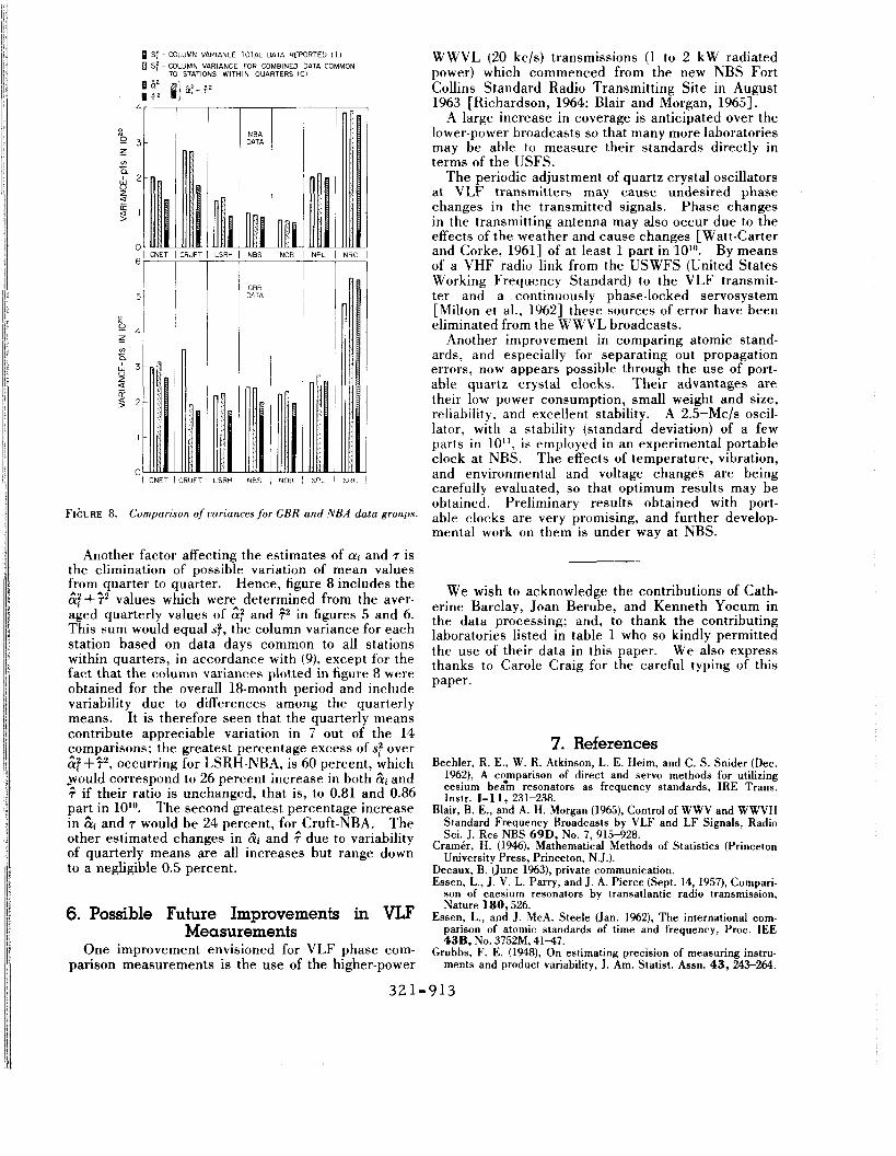
urements common to all stations compared within a given quarter. To estimate the effect of such restric- tion, a comparison was made of the column (station) variances for both restricted (C) and total reported data (T) of each station for the entire 18-month period for both the GBR and NBA transmissions. These data are plotted in figure 8, and the square roots or standard deviations are given in tables 2 and 3 for the GBR and NBA data, respectively. As can be seen there is close agreement in all instances except Cruft- GBR; this exception can be attributed to having only three quarters represented in the restricted data. A new estimate of ai, say Ai, was calculated on the basis of the relative increase or decrease of the restricted data in terms of the total reported data for the overall 18-month period. The previously derived transmitter variance estimate, P, was employed i n these calcu- lations. For the NBA data the new ai differed from -5 to + 6 percent from the previous estimate, di. With the exception of the Cruft data, the new ill for the GBR data differed from - 11 to + 3 percent from Bi. The & calculated from the total reported data for the Cruft GBR data was about three times the &i computed from the quarterly restricted data. This new value, however, is much more in line with that computed from the Cruft NBA data. Thus, with the exception of the Cruft GBR data, the restriction to data days common within quarters has no disturbing effect on the estimation of the atomic standard deviations ai.

1

2t 1 I ;Frl ........... ......... LSR? .....................

0 2 5 2 I

2

<w- 2

.... ...................... .... ---__ '132.h-NBs _ _ I O ___--__

NO8 ............... ................. ;+ .................

:F:.:-/Fl I ..............

, 03 4 1 1 3 4

OTRS 1961 0 7 R S 1962-

FIGURE 7. Comparison of each laboratory standard Gi using either GBR or NBA signals.

32 0-9 12

0 S: -COLUMN VARIANCE TOTAL DATA REPORTED ( T I D S: - COLUMN VARIANCE FOR COMBINED DATA COMMON

TO STATIONS WITHIN QUARTERS IC1

P 0 3 4!7 z

5 t

Q 4 z v)

Q c

h 3 z

3 2 5

I

0 1 CNET

~

NBA DATA

Ilk NBS

~

GER Dr TA

NOB - NPL __

LSRH 1 NBS 1 NOB 1 NPC

F I ~ U R E 8. Comparison of variances f o r GBR and NBA data groups.

Another factor affecting the estimates of ai and 7 is the elimination of possible variation of mean values from quarter to quarter. Hence, figure 8 includes the &: +? values which werc determined from the aver- aged quarterly values of af! and ?2 in figures 5 and 6. This sum would equal sf, the column variance for each station based on data days common to all stations within quarters, in accordance with (9), except for the fact that the column variances plotted in figure 8 were obtained for the overall 18-month period and include variability due to differences among the quarterly means. It is therefore seen that the quarterly means contribute appreciable variation in 7 out of the 14 comparisons; the greatest percentage excess of s,' over ;f+?, occurring for LSRH-NBA, is 60 percent, which _would correspond to 26 percent increase in both &i and ? if their ratio is unchanged, that is, to 0.81 and 0.86 part in lolo. The second greatest percentage increase in 8i and 7 would be 24 percent, for Cruft-NBA. The other estimated changes in Ai and ? due to variability of quarterly means are all increases but range down to a neghgible 0.5 percent.

6. Possible Future Improvements in VLF Measurements

One improvement envisioned for VLF phase com- parison measurements is the use of the higher-power

WWVL (20 kc/s) transmissions (1 to 2 kW radiated power) which commenced from the new NBS Fort Collins Standard Radio Transmitting Site in August 1963 [Richardson, 1964; Blair and Morgan, 19651.

,4 large increase in coverage is anticipated over the lower-power broadcasts so that many more laboratories may be able to measure their standards directly in terms of the USFS.

The periodic adjustment of quartz crystal oscillators at VLF transmitters may cause undesired phase changes in the transmitted signals. Phase changes in the transmitting antenna may also occur due to the effects of the weather and cause changes [Watt-Carter and Corke, 19611 of at least 1 part in lolo. By means of a VHF radio link from the USWFS (United States Working Frequency Standard) to the VLF transmit- ter and a continuously phase-locked servosystem [Milton et al., 19621 these sources of error have been eliminated from the WWVL broadcasts.

Another improvement in comparing atomic stand- ards, and especially for separating out propagation errors, now appears possible through the use of port- able quartz crystal clocks. Their advantages are their low power consumption, small weight and size, reliability, and excellent stability. A 2.5-Mc/s oscil- lator, with a stability (standard deviation) of a few parts in lo", is employed in an experimental portable clock at NBS. The effects of temperature, vibration, and environmental and voltage changes are being carefully evaluated, so that optimum results may be obtained. Preliminary results obtained with port- able clocks are very promising, and further develop- mental work on them is under way at NBS.

We wish to acknowledge the contributions of Cath- erine Barclay, Joan Berube, and Kenneth Yocum in the data processing; and, to thank the contributing laboratories listed in table 1 who so kindly permitted the use of their data in this paper. We also express thanks to Carole Craig for the careful typing of this paper.

7. References Beehler, R. E.. W. R. Atkinson, L. E. Heim, and C. S. Snider (Dec.

1962), A comparison of direct and servo methods for utilizing cesium be& resonators as frequency standards, IRE Trans. Instr. 1-11, 231-238.

Blair, B. E., and A. H. Morgan (1965), Control of WWV and WWVH Standard Frequency Broadcasts by VLF and LF Signals, Radio Sci. J. Res NBS 69D, No. 7,915-928.

Cram&, H. (1946), Mathematical Methods of Statistics (Princeton University Press, Princeton, N.J.).

Decaux, B. (June 1%3), private communication. Essen, L., J. V. L. Parry, and J . A. Pierce (Sept. 14, 1957), Compari-

son of caesium resonators by transatlantic radio transmission, Nature 180,526.

Essen, L., and J . Mc.4. Steele (Jan. 1%2), The international com- parison of atomic standards of time and frequency, Proc. IEE 43B, No. 3752M. 4 1 4 7 .

Grubbs, F. E. (1948), On estimating precision of measuring instru- ments and product variability, J. Am. Statist. Assn. 43, 243-264.

32 1-913

Holloway, J., W. Mainberger, F. H. Reder, G. M. R. Winkler, L. Essen, and J. V. L. Parry (Oct. 1959), Comparison and evalua- tion of cesium atomic beam frequency standards, Proc. IRE 4 7 , 1730-1 736.

Kalra, S. N. (Mar. 1%1), Frequency measurement of standard frequency transmissions, Can. J. Phys. 39,477.

Kartaschoff, P. (Dec. 1962), Operation and improvements of a cesium beam standard having 4-meter interaction length, IRE Trans. on Instr. 1-1 1, 224-230.

Markowitz, W. (April 1961), DCfinition, dktermination et conserva- tion de la seconde, ComitC Consultatif pour la Definition de la Seconde auprks du Comitk International des Poids e t Mesures, 2e session, Annexe 2 (Gauthier-Villars & Cie, Paris), 45-51.

Markowitz, W. (December 1962). The atomic time scale, IRE Trans. on Instr. 1-11, 239-242.

Markowitz, W. (July-August 1964). International Frequency and Clock Synchronization, Frequency, 2, No. 4,30-31.

Milton, J. B., R. L. Fey, and A. H. Morgan (March 17, 1962). Remote phase control of radio station WWVL, Nature 193, No. 4820, 1063-1064.

Mitchell, A. M. J. (June 22, 1963). Frequency comparison of atomic standards by radio links, Nature 198, No. 4886,1155-1158.

Morgan, A. H., and D. H. Andrews (April 1%1), MCthodes et.Tech- niques de contr6le des ondes kilomktriques et myriamktriques aux Boulder Laboratories, ComitC Consultatif pour la DCfinition de la Seconde auprks du Comiti International des Poids et Mesures, 2e session, Annexe 6 (Gauthier-Villars & C'", Paris), 68-72.

Morgan, A. H., B. E. Blair, and E. L. Crow (1%5), International comparison of atomic frequency standards via VLF radio signals, Progress in Radio Science 1960-1%3, 1, Radio Standards and Measurements, (Elsevier Publishing Company, Amsterdam/ London/New York, 1%5), 40.

NBS (Dec. 1964), World sets atomic definition of time, NBS Tech. News Bull. 48,20!+210.

NPL (1963). Report for year 1962, standards division, electrical and frequency measurements, NPL (Teddington, England), 217.

NPL (1%4), Report for year 1963, standards division, electrical and frequency measurements, NPL (Teddington, England), 216, 217.

Pierce, J. A. (June 1957), Intercontinental frequency comparisons by very low frequency radio transmission, Proc. IRE 45, 704-803.

Pierce, J. A., G. M. R. Winkler, and R. L. Corke (September 10, 1960), The 'GBR Experiment': A trans-Atlantic frequency com- parison between caesium-controlled oscillators, Nature 187, No. 4741,914-916.

Pierce, J. A. (July 1963), private communication. Richardson, J. M., R. E. Beehler, R. C. Mockler, and R. L. Fey (April

1961), Les Ctalons atomiques de frkquence au N.B.S., ComitC Consultatif pour la DCfinition de la Seconde auprks du ComitC International des Poids et Mesures, 2e session, Annexe 5 (Gauthier- Villars & Cie, Pans), 57-67.

Richardson, J . M. (January 1964). Establishment of new facilities for WWVL and WWVB, Radio Sci. J. Res. NBS 68D, No. 1, 135.

Watt-Carter, D. E., and R. L. Corke (September 23,1961), VLF trans- mitting'system phase transfer variations, Nature 191, No. 4795, 1286.

Note added in proof. A mistake in the calculation of the rms weighted average b? for LSRH using GBR transmissions has been discovered; it shouid be 0.0156 rather than 0.156, resulting in an rms average 6, of 0.12 rather than 0.39 (parts in 103. The change should be made in the abstract, the table on page 911, and the table within figure 5. The apparently considerable change is of doubtful significance because, as stated on page 910, the confidence limits on this ai are about 100 percent above and below the estimate 6,. In fact the further data for 1%3 and 1964 (502 days) yield 0.43, and when these are combined with the 244 days of data in 1%1 and 1%2, the overall rms average 6, is 0.36.

(Paper 69D7-524)

322-914