VituixCAD - Kimmo Saunisto · VituixCAD Page 3 of 44 Version 1.1 VituixCAD General information...
44
VituixCAD The Loudspeaker Simulation Tool by Kimmo Saunisto Online Manual Copyright © Joni Laakso 2018 [email protected] 2018-03-12
-
Upload
nguyencong -
Category
Documents
-
view
216 -
download
0
Transcript of VituixCAD - Kimmo Saunisto · VituixCAD Page 3 of 44 Version 1.1 VituixCAD General information...

VituixCAD
The Loudspeaker Simulation Tool
by Kimmo Saunisto
Online Manual
Copyright © Joni Laakso 2018
2018-03-12
VituixCAD Page 2 of 44 Version 1.1
Contents
VituixCAD .............................................................................................................................................................................. 3
General information ......................................................................................................................................................... 3
System requirements ....................................................................................................................................................... 3
Installation and Upgrade .................................................................................................................................................. 3
Support ............................................................................................................................................................................. 3
Quick User Guide .................................................................................................................................................................. 4
Preface ............................................................................................................................................................................. 4
Checklist for designing a loudspeaker .............................................................................................................................. 4
Detailed descriptions ........................................................................................................................................................... 6
Main window .................................................................................................................................................................... 6
Menus ............................................................................................................................................................................... 6
Drivers tab ........................................................................................................................................................................ 7
Crossover tab ................................................................................................................................................................... 9
Dashboard (Graphs) ....................................................................................................................................................... 13
Optimizer ........................................................................................................................................................................ 16
Schema window ............................................................................................................................................................. 18
Parts list .......................................................................................................................................................................... 18
Impulse response ........................................................................................................................................................... 19
Power dissipation ........................................................................................................................................................... 20
Options ........................................................................................................................................................................... 21
Enclosure tool ................................................................................................................................................................. 24
Driver database .......................................................................................................................................................... 24
Driver configuration ................................................................................................................................................... 27
Radiator type .............................................................................................................................................................. 28
Tabs ............................................................................................................................................................................ 28
Export functions ......................................................................................................................................................... 31
Dashboard (Graphs) ................................................................................................................................................... 31
Merger tool .................................................................................................................................................................... 32
Calculator tool ................................................................................................................................................................ 34
Multiple output .......................................................................................................................................................... 34
Single output .............................................................................................................................................................. 36
Additional options ...................................................................................................................................................... 37
Graph .......................................................................................................................................................................... 38
Diffraction tool ............................................................................................................................................................... 39
SPL Trace ........................................................................................................................................................................ 41
Auxiliary calculator ......................................................................................................................................................... 43
VituixCAD Page 3 of 44 Version 1.1
VituixCAD
General information
VituixCAD is loudspeaker simulation software. Design philosophy is to simulate loudspeaker behavior in full space.
Even though emphasis is on power response, polar responses and directivity index, it is possible to design a
loudspeaker without comprehensive angled measurements. This is not encouraged though.
VituixCAD offers possibility to design and simulate up to 6-way loudspeaker. Each way can have up to 4 drivers in
different configurations.
Software package includes everything one needs for simulating and designing a loudspeaker. Additional to
simulator itself, there is enclosure simulator, response merger and advanced calculator tool included.
This document is divided into three sections; general information about the software, quick user guide and detailed
descriptions of tools, views and theory behind the software.
System requirements
VituixCAD is tested on Windows XP, 7, 8 and 10.
Microsoft .NET Framework 4 or newer. Tested up to 4.7.1.
Minimum screen resolution is 1024x768 (4:3) or 1280x720 (16:9), but 1600x900 or more is recommended.
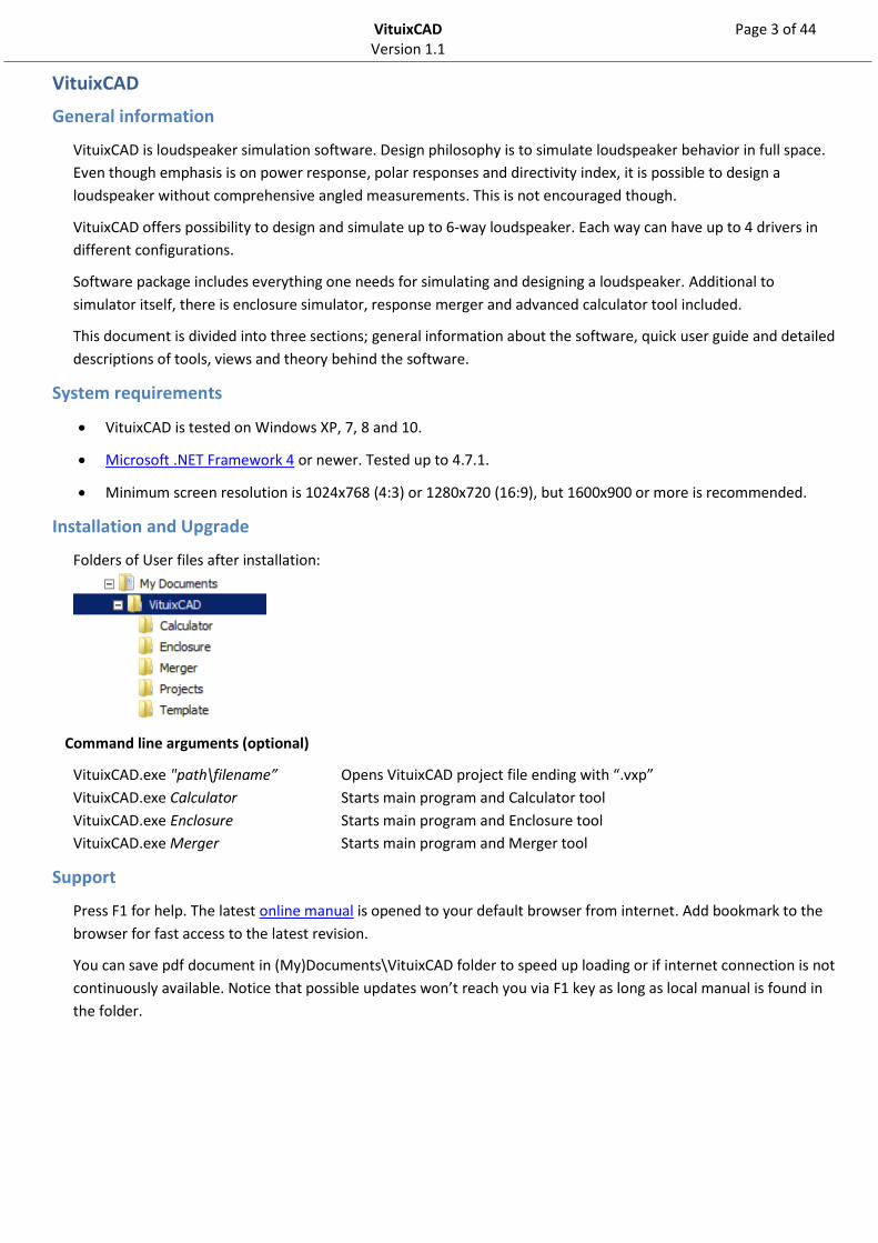
Installation and Upgrade
Folders of User files after installation:
Command line arguments (optional)
VituixCAD.exe "path\filename” Opens VituixCAD project file ending with “.vxp”
VituixCAD.exe Calculator Starts main program and Calculator tool
VituixCAD.exe Enclosure Starts main program and Enclosure tool
VituixCAD.exe Merger Starts main program and Merger tool
Support
Press F1 for help. The latest online manual is opened to your default browser from internet. Add bookmark to the
browser for fast access to the latest revision.
You can save pdf document in (My)Documents\VituixCAD folder to speed up loading or if internet connection is not
continuously available. Notice that possible updates won’t reach you via F1 key as long as local manual is found in
the folder.

VituixCAD Page 4 of 44 Version 1.1
Quick User Guide
Preface
This user guide is a chronological walkthrough on how to design a loudspeaker with VituixCAD. Commonly, design
process starts with deciding enclosure size, drivers, radiator type, alignment etc. Enclosure tool is used for
simulating enclosures, different radiator types and alignments. Next step is to have comprehensive set of acoustic
and electrical measurements of the construction. Merger tool is used for combining far field and near field
responses. After these prerequisites are met, simulation phase can be started. Whether Your goal is to design a
speaker with or without interim listening tests, You’ll need quality control of some sort. Some prefer their ears,
some prefer measurements. If a loudspeaker measures perfectly, but sounds worse than anything You’ve ever
heard, something is terribly wrong. This guide will not teach You how to listen a loudspeaker, but will cover basic
QC steps and VituixCAD Calculator, which can be used for various calculations and manipulations for measured
data.
Building prototypes and crossovers are not covered in this guide. This guide will also assume You have suitable
measurement gear and software and understanding about how to measure loudspeaker drivers for design
purposes. More detailed description of tools and views are provided in Detailed descriptions part of this document.
Checklist for designing a loudspeaker Investigate acoustic parameters, dimensions, materials and speaker placement possibilities of the listening room. It is wise to fix issues of bad environment (the room) first rather than trying to handle everything with massive and complex speaker design. Basic engineering
Decide acoustic design; type and amount of directivity, radiator types, ways, driver size and count.
Estimate possible sensitivity range and crossover frequency ranges.
Select initial drivers and directivity components to reach previous targets
Simulate low frequency radiators with Enclosure tool
Simulate baffle diffraction and export cabinet impact response
Design the cabinet. Construction
Build flexible prototype or final cabinet depending on uncertainties in the design
Connect temporary cables to individual drivers or driver groups for acoustical and electrical measurements.
Measurements
Prepare turning table for polar response measurements. Manual turning table is easy to make and fast to use for example with Clio 10/11 or ARTA 1.9.
Choose directions for off-axis measurements. You are not forced to measure full or half circle around the speaker with constant 5 or 10 deg steps, but it is highly recommended. Simulation is possible with less than 10 directions per axis. Don’t waste Your chance to get all measured data at once. There is no need to measure vertical axis if vertical measurement would be “equal enough” to horizontal measurement. For example full range driver in the center of square box is symmetrical in both directions.
Measure polar response of each driver or driver group as far field measurement. Use equal off-axis angles for all drivers. Don’t let measuring program to corrupt timing: use semi-dual (or full dual) channel measurement to lock time reference to mic capsule. Measure time-windowed responses from the same or at least known/measured distance to the reference point to maintain common time reference with different ways & drivers.
Measure near field responses of midrange and woofer cone(s) and port(s) if anechoic environment is not available. Arrange radiator to half space to avoid baffle loss. Some amount of baffle loss exists with small cabinets in full space even if measurement distance is less than 8 mm. Use same output voltage with far field measurement (if possible without clipping or excessive distortion) to help merging of near field and far field measurements.
Measure impedance responses of each driver or driver group.
VituixCAD Page 5 of 44 Version 1.1
Merge and manipulate response data
Merge far field and near field responses with Merger tool if you didn’t measure low frequency radiators (<300 Hz) from far field in anechoic environment.
Include cabinet impact response (from diffraction simulator) in near field responses.
Export merged responses as separate txt-files (or as extended data file if smoothing is not needed).
Smooth responses with Calculator tool if necessary. Simulate loudspeaker with VituixCAD
Create new empty project and enter Description
Insert number of ways
Select number of drivers and electrical connection
Enter driver names, locations and possible rotation or inclination
Insert frequency responses
Insert impedance response
Outline rough targets for axial response and power response
Outline rough targets for axial responses per way
Design the crossover Insert filter blocks manually or by the Wizard Adjust parameter/component values of filter blocks manually or by the Wizard Play with circuit topologies and parameter/component values until axial response, power response,
directivity index, polar responses and impedance response meet Your targets. Save project periodically. Save as… most promising intermediate results.
Built and install crossover Quality control
Mandatory QC-measurements Angled measurements in horizontal and vertical planes, at least 30 deg steps Impedance response Listen to Your favorite tracks
If you are not satisfied -> back to drawing board Additional QC-measurements
Excess group delay Harmonic distortion Intermodulation distortion Compression Acoustic compatibility to your listening room; room response, clarity parameters.
VituixCAD Page 6 of 44 Version 1.1
Detailed descriptions
Main window
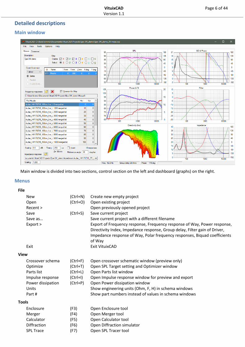
Main window is divided into two sections, control section on the left and dashboard (graphs) on the right.
Menus
File
New (Ctrl+N) Create new empty project Open (Ctrl+O) Open existing project Recent > Open previously opened project Save (Ctrl+S) Save current project Save as… Save current project with a different filename Export > Export of Frequency response, Frequency response of Way, Power response,
Directivity Index, Impedance response, Group delay, Filter gain of Driver, Impedance response of Way, Polar frequency responses, Biquad coefficients of Way
Exit Exit VituixCAD
View
Crossover schema (Ctrl+F) Open crossover schematic window (preview only) Optimize (Ctrl+T) Open SPL Target setting and Optimizer window Parts list (Ctrl+L) Open Parts list window Impulse response (Ctrl+I) Open Impulse response window for preview and export Power dissipation (Ctrl+P) Open Power dissipation window Units Show engineering units (Ohm, F, H) in schema windows Part # Show part numbers instead of values in schema windows
Tools
Enclosure (F3) Open Enclosure tool Merger (F4) Open Merger tool Calculator (F5) Open Calculator tool Diffraction (F6) Open Diffraction simulator SPL Trace (F7) Open SPL Tracer tool
VituixCAD Page 7 of 44 Version 1.1
Auxiliary (F8) Open Auxiliary calculator
Options
(Alt+O) Open Options window
Help
Online Manual EN (F1) Open user manual in English Online Manual DE Open user manual in German About Information about VituixCAD. View changelog.
Drivers tab
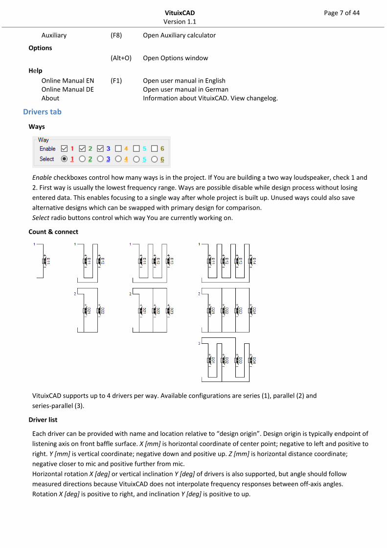
Ways
Enable checkboxes control how many ways is in the project. If You are building a two way loudspeaker, check 1 and
2. First way is usually the lowest frequency range. Ways are possible disable while design process without losing
entered data. This enables focusing to a single way after whole project is built up. Unused ways could also save
alternative designs which can be swapped with primary design for comparison.
Select radio buttons control which way You are currently working on.
Count & connect
VituixCAD supports up to 4 drivers per way. Available configurations are series (1), parallel (2) and
series-parallel (3).
Driver list
Each driver can be provided with name and location relative to “design origin”. Design origin is typically endpoint of
listening axis on front baffle surface. X [mm] is horizontal coordinate of center point; negative to left and positive to
right. Y [mm] is vertical coordinate; negative down and positive up. Z [mm] is horizontal distance coordinate;
negative closer to mic and positive further from mic.
Horizontal rotation X [deg] or vertical inclination Y [deg] of drivers is also supported, but angle should follow
measured directions because VituixCAD does not interpolate frequency responses between off-axis angles.
Rotation X [deg] is positive to right, and inclination Y [deg] is positive to up.

VituixCAD Page 8 of 44 Version 1.1
Multiple drivers should be entered as a single driver if they are measured in the prototype cabinet as a package; all
connected to power amplifier at the same time. Location is entered as a difference between measurement and
design origins.
Example 1: Location (X,Y,Z) = (0,0,0) if multiple driver package is measured on design (listening) axis.
Example 2: Location (X,Y,Z) = (0,-400,0) if multiple driver package is measured 400 mm below design (listening) axis.
Frequency responses
Add driver’s frequency responses by clicking folder button or dropping files into response list. You can use
individual off-axis responses or LspCAD extended format file created with Merger tool. Delete button clears
response list. Drivers #2-4 are able to use all measurements of driver #1 by checking Common for Way.
Maximum of 74 frequency response measurements per driver is supported. Loaded responses are verified against
other ways & drivers. Directions which are common for all enabled ways and drivers are included in simulation.
Frequency responses can be scaled (dB), delayed (± µs) and polarity can be inverted with controls below frequency
response list. Hor and Ver angle can be modified by entering new value to the field if program fails to parse value
from the filename or measurements are swapped intentionally.
Reference angle is direction in horizontal plane which is shown as axial response in SPL, Power & DI and Phase
response graphs. Also directivity index calculation is using Reference angle as main axis. Optimizing to single
off-axis direction is useful if axial response is bad or not representative or measurement data is poor and accurate
power response approximation is not available. Default value is 0 deg hor.
Impedance response
Select impedance response file for a driver(s) by clicking folder button or dropping file into text box.
Impedance response can be scaled as well with a multiplier. If multiple drivers are entered as a single driver, scaled
impedance response should represent total impedance of the driver package.
Supported frequency and impedance response file types
VituixCAD supports tab, space or semicolon delimited .txt or .frd or .zma (for impedance). Following software
exports are supported:
AudioTools
ARTA, LIMP
Clio
Edge
FRD tools

VituixCAD Page 9 of 44 Version 1.1
HOLM Impulse
justMLS, LspCAD 6 extended format
Klippel
LspLAB
REW
SoundEasy
XSim
Crossover tab
Filter schema
Maximum of 15 filter blocks can be assigned for each way via Crossover block menu or a wizard. Drag & drop from
menu to schema is available.
Filter blocks can be moved by Drag & drop, or forward and backwards within the same net by clicking arrow
buttons on the right. Single block can be copied by Ctrl + Drag & drop. Selected block can be removed by clicking
delete button . Filter network can be deleted by pop-up menu (right click). Network can be Copy - Pasted to
another way or project by pop-up menu. Selected block can be bypassed by checkbox below B button on the right.
Bypass status of all blocks on the selected way is inverted by clicking B button. Bypassed blocks are grayed in
schema view.
Up to ten most recent crossover changes and situations before parameter adjustment can be restored with Undo
(Ctrl+Z) command in context menu of filter schema. Way settings such as gain, delay and invert, and every single
parameter change is not saved to undo buffer.
Schema view can be expanded over Block menu, Connection menu and Wizard by clicking expand button .
Schema window showing total crossover without bypassed blocks and disabled ways can be opened by selecting
View→Crossover schema (Ctrl+F).
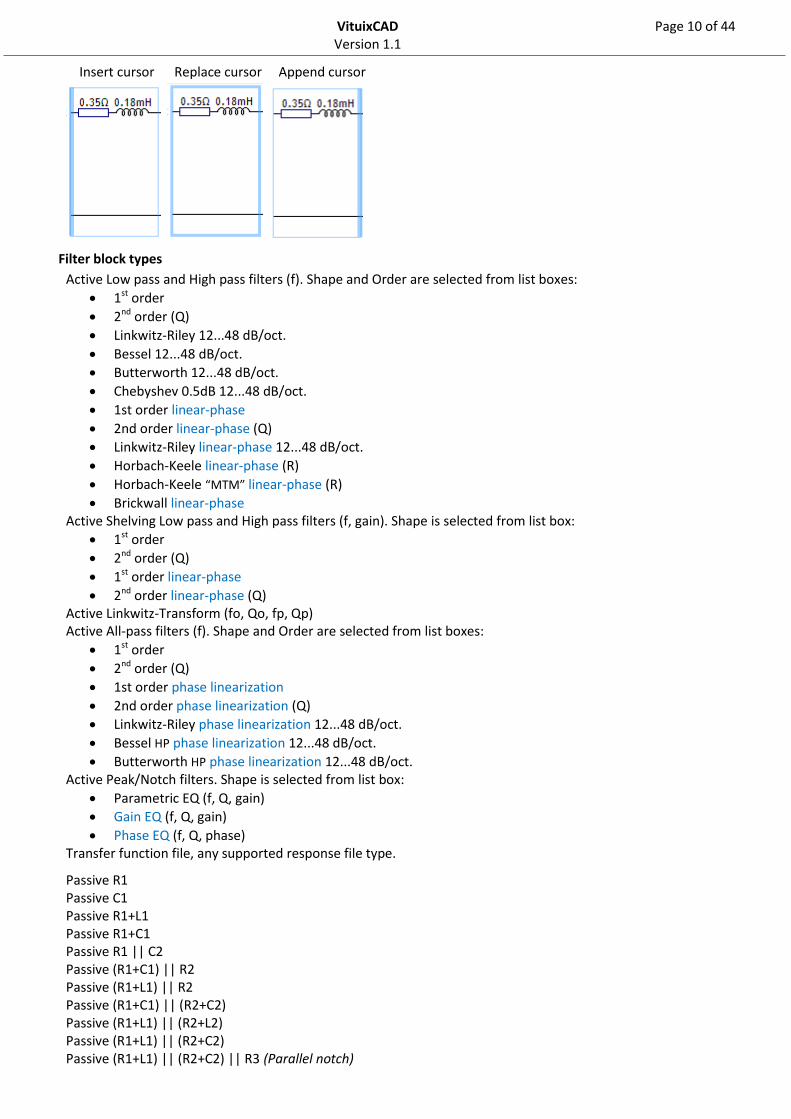
Insert/Replace/Append mode
Filter blocks are placed in the schema according mode selection. In Insert mode new blocks are placed under the
cursor without overwriting existing blocks. Replace mode overwrites the block under the cursor. Replace mode
activates automatically when any filter block in the schema is clicked. In Append mode new blocks are added right
after currently selected block. You can toggle between modes by radio buttons or pressing Insert key when mouse
cursor is over schema.
VituixCAD Page 10 of 44 Version 1.1
Insert cursor Replace cursor Append cursor
Filter block types
Active Low pass and High pass filters (f). Shape and Order are selected from list boxes:
1st order
2nd order (Q)
Linkwitz-Riley 12...48 dB/oct.
Bessel 12...48 dB/oct.
Butterworth 12...48 dB/oct.
Chebyshev 0.5dB 12...48 dB/oct.
1st order linear-phase
2nd order linear-phase (Q)
Linkwitz-Riley linear-phase 12...48 dB/oct.
Horbach-Keele linear-phase (R)
Horbach-Keele “MTM” linear-phase (R)
Brickwall linear-phase Active Shelving Low pass and High pass filters (f, gain). Shape is selected from list box:
1st order
2nd order (Q)
1st order linear-phase
2nd order linear-phase (Q) Active Linkwitz-Transform (fo, Qo, fp, Qp) Active All-pass filters (f). Shape and Order are selected from list boxes:
1st order
2nd order (Q)
1st order phase linearization
2nd order phase linearization (Q)
Linkwitz-Riley phase linearization 12...48 dB/oct.
Bessel HP phase linearization 12...48 dB/oct.
Butterworth HP phase linearization 12...48 dB/oct. Active Peak/Notch filters. Shape is selected from list box:
Parametric EQ (f, Q, gain)
Gain EQ (f, Q, gain)
Phase EQ (f, Q, phase) Transfer function file, any supported response file type.
Passive R1 Passive C1 Passive R1+L1 Passive R1+C1 Passive R1 || C2 Passive (R1+C1) || R2 Passive (R1+L1) || R2 Passive (R1+C1) || (R2+C2) Passive (R1+L1) || (R2+L2) Passive (R1+L1) || (R2+C2) Passive (R1+L1) || (R2+C2) || R3 (Parallel notch)
VituixCAD Page 11 of 44 Version 1.1
Passive R1+L1+C1 (Series notch) Passive (R1+L1+C1) || R2 Passive Lattice all-pass Passive (R1+L1+C1) || (R2+L2) || R3 Passive (R1+L1+C1) || (R2+C2) || R3 Passive (R1+L1+C1) || (R2+L2+C2) || R3
Important! Active filters having blue text are NOT minimum-phase. Blocks in the schema views have ‘FIR’ text for
information. Convolver plugin or DSP device with FIR features is needed for real life application. Transfer function
of active filters per way can be exported as impulse response in wav or txt file format. See section
Impulse response.
Biquad coefficients
Active IIR blocks can be exported or copied to clipboard as digital biquad filter coefficients b0, b1, b2, a1, a2:
Format is compatible with miniDSP Xover/PEQ Advanced view. For example 3rd order Butterworth LP 1000 Hz:
biquad1,
b0=0.004015505022858,
b1=0.008031010045716,
b2=0.004015505022858,
a1=1.86140844453211,
a2=-0.877470464623539,
biquad2,
b0=0.061511768503622,
b1=0.061511768503622,
b2=0,
a1=0.876976462992757,
a2=0,
Biquads of Way can be exported as text file with File -> Export -> Biquad coefficients of Way.
Coefficients can be copied to clipboard with context menu of filter schema (right click):
Copy Biquad coefficients of selected Block (Ctrl+B)
Copy Biquad coefficients of Way (Ctrl+W)
Note! Select correct sample rate from Impulse response window before copying/exporting biquads. FIR, transfer
function file, passive and by-passed blocks are ignored. Stability of biquad filters is not checked.
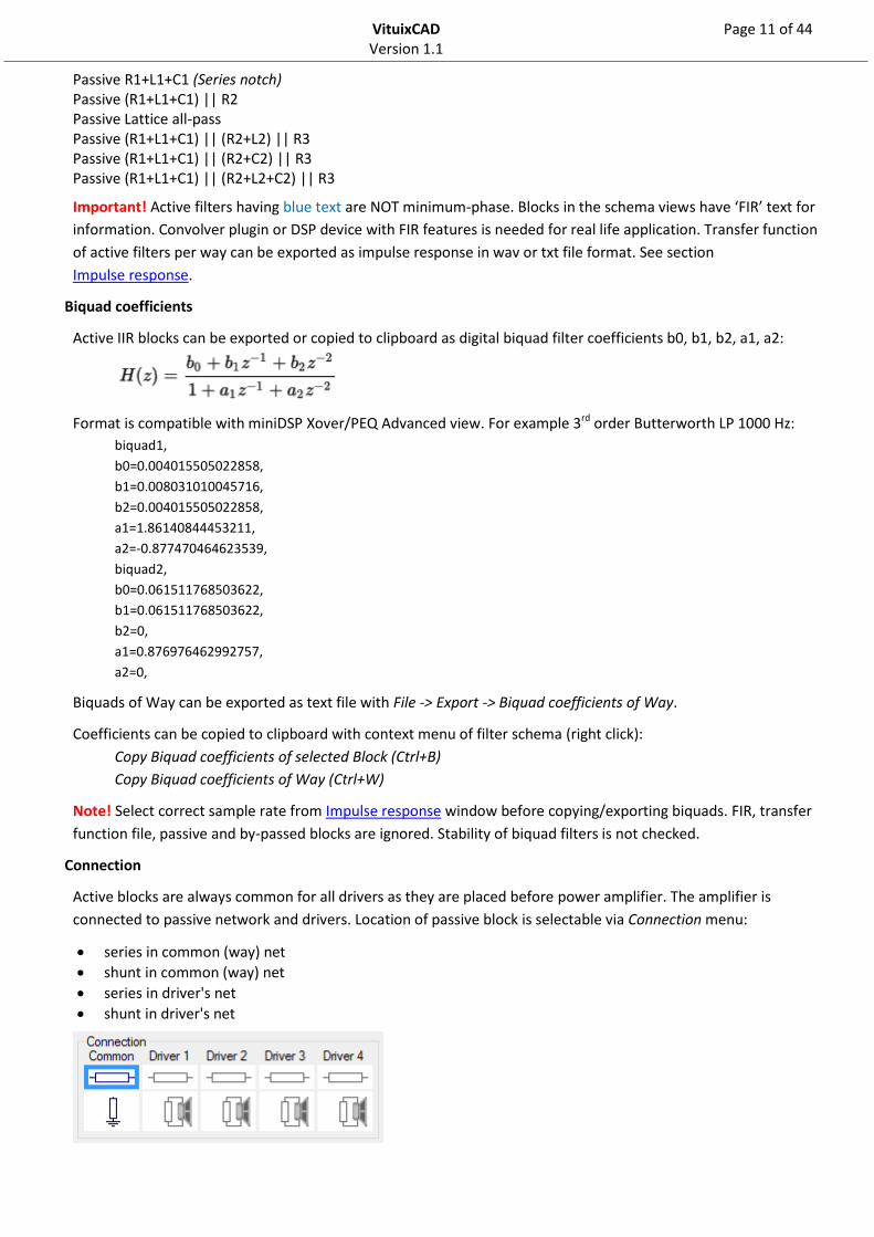
Connection
Active blocks are always common for all drivers as they are placed before power amplifier. The amplifier is
connected to passive network and drivers. Location of passive block is selectable via Connection menu:
series in common (way) net
shunt in common (way) net
series in driver's net
shunt in driver's net
VituixCAD Page 12 of 44 Version 1.1
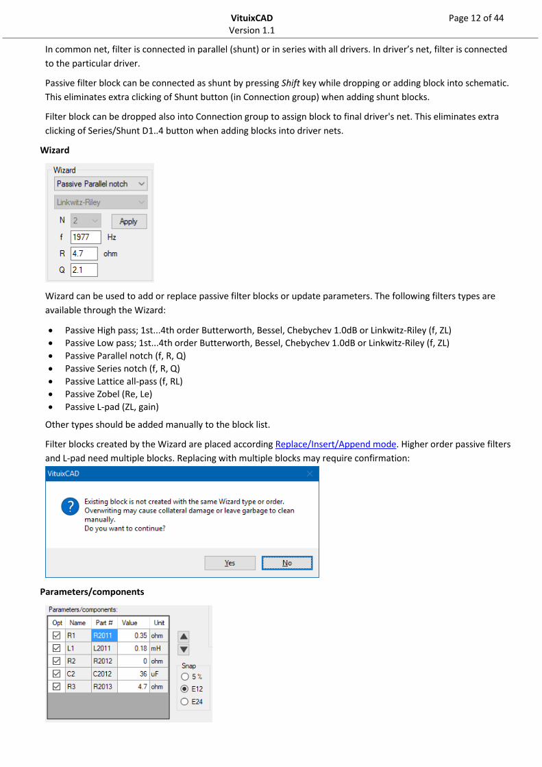
In common net, filter is connected in parallel (shunt) or in series with all drivers. In driver’s net, filter is connected
to the particular driver.
Passive filter block can be connected as shunt by pressing Shift key while dropping or adding block into schematic.
This eliminates extra clicking of Shunt button (in Connection group) when adding shunt blocks.
Filter block can be dropped also into Connection group to assign block to final driver's net. This eliminates extra
clicking of Series/Shunt D1..4 button when adding blocks into driver nets.
Wizard
Wizard can be used to add or replace passive filter blocks or update parameters. The following filters types are
available through the Wizard:
Passive High pass; 1st...4th order Butterworth, Bessel, Chebychev 1.0dB or Linkwitz-Riley (f, ZL)
Passive Low pass; 1st...4th order Butterworth, Bessel, Chebychev 1.0dB or Linkwitz-Riley (f, ZL)
Passive Parallel notch (f, R, Q)
Passive Series notch (f, R, Q)
Passive Lattice all-pass (f, RL)
Passive Zobel (Re, Le)
Passive L-pad (ZL, gain)
Other types should be added manually to the block list.
Filter blocks created by the Wizard are placed according Replace/Insert/Append mode. Higher order passive filters
and L-pad need multiple blocks. Replacing with multiple blocks may require confirmation:
Parameters/components

VituixCAD Page 13 of 44 Version 1.1
Selecting filter block opens corresponding parameters/components to the list. Component values can be entered
directly to the Value field. Additionally, component value can be increased/decreased by Alt+Up/Down key or
arrow buttons on the right or mouse wheel. Increment is defined by component Snap value. Available values are
5 %, E12 or E24.
Parameter will be included in frequency response optimizing if Opt field is checked. Otherwise parameter is
excluded and existing value locked. See Optimize.
Way # settings
Adjustable active gain [dB] and DSP delay [µs] are available for each way. Gain and delay can be adjusted
automatically with optimizer by checking the label. See Optimize. Polarity of the way can be inverted by Invert
checkbox. Enabled is a mirror twin with checkbox on Drivers tab.
Dashboard (Graphs)
SPL
By default, SPL graph shows total SPL, total SPL target, SPL per way, SPL per individual driver and total phase. All
lines are responses to Reference angle, see Frequency responses. Color coding for traces:
Total SPL: black Total phase: gray. Optional, disabled by unchecking Show Normal phase in context menu. Minimum phase: lime. Optional, enabled by checking Show Minimum phase in context menu. Excess phase: steel blue. Optional, enabled by checking Show Excess phase in context menu. SPL per way: red, green, blue, orange, cyan, olive SPL per individual driver: light red, light green, light blue, light orange, light cyan, light olive Adjustable SPL target: magenta. Optional, disabled by unchecking Show Target line in context menu.
SPL Target can be adjusted by dragging the line ends with mouse while Shift or Control key is pressed. This is target
line for axial response optimizing. See Optimize.
Zooming
Every graph can be zoomed to full size and back to dashboard by double clicking in middle of the chart area.
VituixCAD Page 14 of 44 Version 1.1
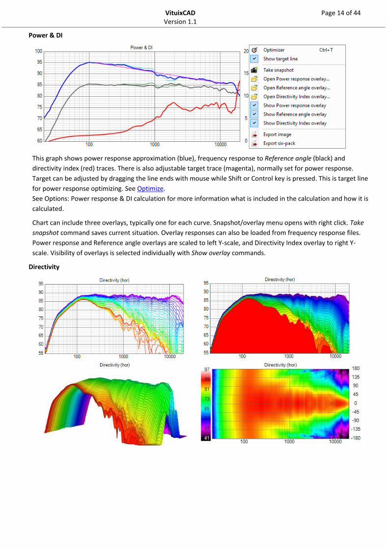
Power & DI
This graph shows power response approximation (blue), frequency response to Reference angle (black) and
directivity index (red) traces. There is also adjustable target trace (magenta), normally set for power response.
Target can be adjusted by dragging the line ends with mouse while Shift or Control key is pressed. This is target line
for power response optimizing. See Optimize.
See Options: Power response & DI calculation for more information what is included in the calculation and how it is
calculated.
Chart can include three overlays, typically one for each curve. Snapshot/overlay menu opens with right click. Take
snapshot command saves current situation. Overlay responses can also be loaded from frequency response files.
Power response and Reference angle overlays are scaled to left Y-scale, and Directivity Index overlay to right Y-
scale. Visibility of overlays is selected individually with Show overlay commands.
Directivity

VituixCAD Page 15 of 44 Version 1.1
Directivity chart options context menu (right click on the graph):
This graph shows directivity simulation as line chart, area chart, surface chart, polar map (aka heat map) or polar
chart. You must have frequency responses to all angles (common for all ways and drivers) You want to show in this
graph. Response to Reference angle is emphasized with thick line.
Rotation, inclination, zooming and panning are available for surface chart with dragging and wheeling with a
mouse. Pan graph by pressing Ctrl-key while dragging. Limits for rotation and inclination are 10…170 deg.
Checking Polar chart will show polar plot at frequency selected with horizontal scrollbar.
Checking Negative angles in front will invert angle-axis of the plot.
Checking Normalized will show flat response to Reference angle.
Checking Contour lines will show edges of level ranges with Polar map. Level steps are initially 3 dB.
Group delay & Phase
This graph shows total group delay (black) and phase response of individual drivers to Reference angle. Color
coding follows the same rules as defined in Ways section. Optional Excess group delay (steel blue) is enabled by
checking Show Excess group delay in context menu. Group delay can be hidden by unchecking Show Normal group
delay.
VituixCAD Page 16 of 44 Version 1.1
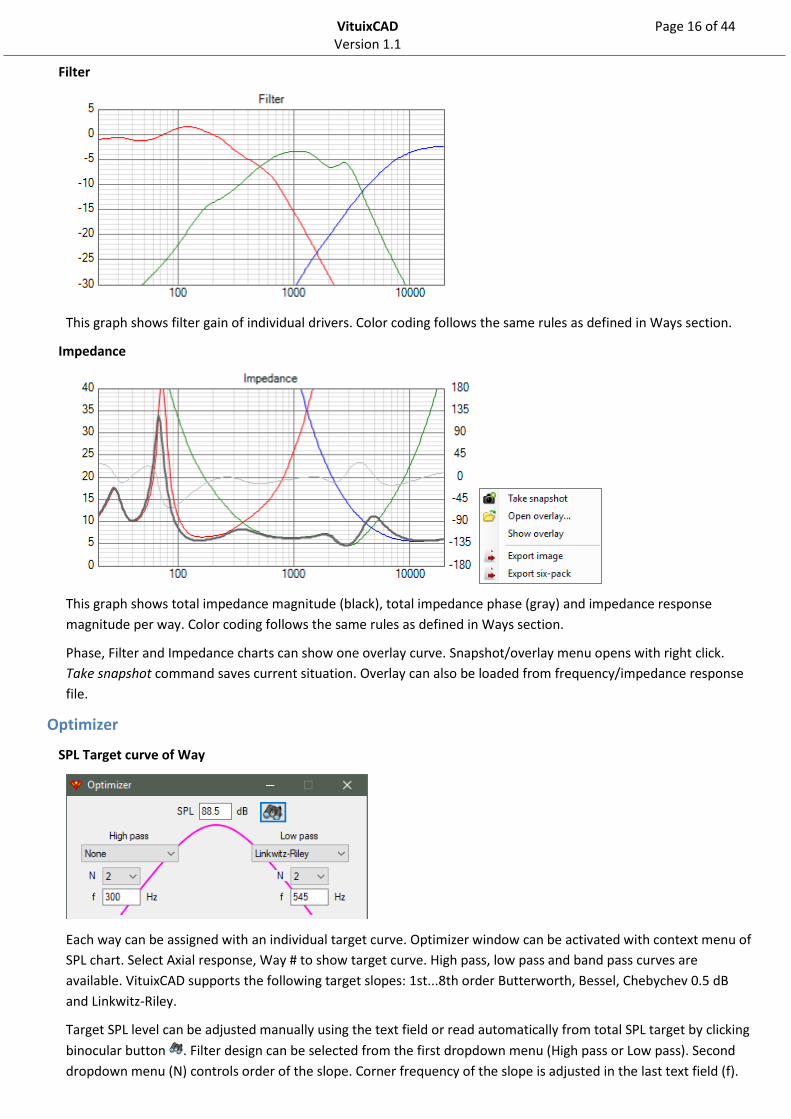
Filter
This graph shows filter gain of individual drivers. Color coding follows the same rules as defined in Ways section.
Impedance
This graph shows total impedance magnitude (black), total impedance phase (gray) and impedance response
magnitude per way. Color coding follows the same rules as defined in Ways section.
Phase, Filter and Impedance charts can show one overlay curve. Snapshot/overlay menu opens with right click.
Take snapshot command saves current situation. Overlay can also be loaded from frequency/impedance response
file.
Optimizer
SPL Target curve of Way
Each way can be assigned with an individual target curve. Optimizer window can be activated with context menu of
SPL chart. Select Axial response, Way # to show target curve. High pass, low pass and band pass curves are
available. VituixCAD supports the following target slopes: 1st...8th order Butterworth, Bessel, Chebychev 0.5 dB
and Linkwitz-Riley.
Target SPL level can be adjusted manually using the text field or read automatically from total SPL target by clicking
binocular button . Filter design can be selected from the first dropdown menu (High pass or Low pass). Second
dropdown menu (N) controls order of the slope. Corner frequency of the slope is adjusted in the last text field (f).
VituixCAD Page 17 of 44 Version 1.1
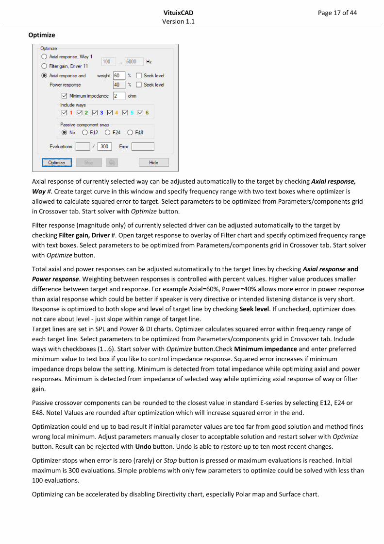
Optimize
Axial response of currently selected way can be adjusted automatically to the target by checking Axial response,
Way #. Create target curve in this window and specify frequency range with two text boxes where optimizer is
allowed to calculate squared error to target. Select parameters to be optimized from Parameters/components grid
in Crossover tab. Start solver with Optimize button.
Filter response (magnitude only) of currently selected driver can be adjusted automatically to the target by
checking Filter gain, Driver #. Open target response to overlay of Filter chart and specify optimized frequency range
with text boxes. Select parameters to be optimized from Parameters/components grid in Crossover tab. Start solver
with Optimize button.
Total axial and power responses can be adjusted automatically to the target lines by checking Axial response and
Power response. Weighting between responses is controlled with percent values. Higher value produces smaller
difference between target and response. For example Axial=60%, Power=40% allows more error in power response
than axial response which could be better if speaker is very directive or intended listening distance is very short.
Response is optimized to both slope and level of target line by checking Seek level. If unchecked, optimizer does
not care about level - just slope within range of target line.
Target lines are set in SPL and Power & DI charts. Optimizer calculates squared error within frequency range of
each target line. Select parameters to be optimized from Parameters/components grid in Crossover tab. Include
ways with checkboxes (1…6). Start solver with Optimize button.Check Minimum impedance and enter preferred
minimum value to text box if you like to control impedance response. Squared error increases if minimum
impedance drops below the setting. Minimum is detected from total impedance while optimizing axial and power
responses. Minimum is detected from impedance of selected way while optimizing axial response of way or filter
gain.
Passive crossover components can be rounded to the closest value in standard E-series by selecting E12, E24 or
E48. Note! Values are rounded after optimization which will increase squared error in the end.
Optimization could end up to bad result if initial parameter values are too far from good solution and method finds
wrong local minimum. Adjust parameters manually closer to acceptable solution and restart solver with Optimize
button. Result can be rejected with Undo button. Undo is able to restore up to ten most recent changes.
Optimizer stops when error is zero (rarely) or Stop button is pressed or maximum evaluations is reached. Initial
maximum is 300 evaluations. Simple problems with only few parameters to optimize could be solved with less than
100 evaluations.
Optimizing can be accelerated by disabling Directivity chart, especially Polar map and Surface chart.

VituixCAD Page 18 of 44 Version 1.1
Schema window
Units Part #
Schema window shows the total crossover network without disabled ways and bypassed filter blocks. Visibility of
values and units or component names is controlled by Units and Part # in View menu.
Parts list
Parts list shows passive filter components and values as text. List can be copied (right click, Select All, Copy) and
pasted to Your favorite spreadsheet or text editor. Please be careful when copy - pasting, resistance of coils are
shown as individual resistors or included in value of actual resistor in series with the coil.
VituixCAD Page 19 of 44 Version 1.1
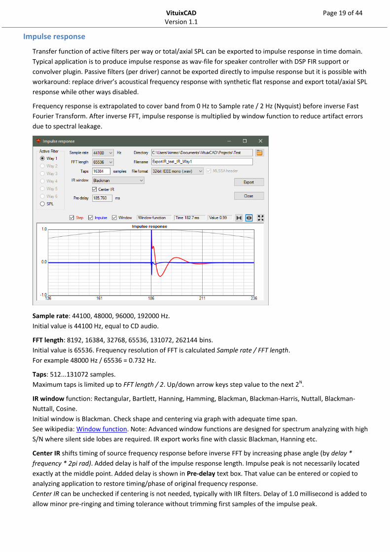
Impulse response
Transfer function of active filters per way or total/axial SPL can be exported to impulse response in time domain.
Typical application is to produce impulse response as wav-file for speaker controller with DSP FIR support or
convolver plugin. Passive filters (per driver) cannot be exported directly to impulse response but it is possible with
workaround: replace driver’s acoustical frequency response with synthetic flat response and export total/axial SPL
response while other ways disabled.
Frequency response is extrapolated to cover band from 0 Hz to Sample rate / 2 Hz (Nyquist) before inverse Fast
Fourier Transform. After inverse FFT, impulse response is multiplied by window function to reduce artifact errors
due to spectral leakage.
Sample rate: 44100, 48000, 96000, 192000 Hz.
Initial value is 44100 Hz, equal to CD audio.
FFT length: 8192, 16384, 32768, 65536, 131072, 262144 bins.
Initial value is 65536. Frequency resolution of FFT is calculated Sample rate / FFT length.
For example 48000 Hz / 65536 = 0.732 Hz.
Taps: 512...131072 samples.
Maximum taps is limited up to FFT length / 2. Up/down arrow keys step value to the next 2N.
IR window function: Rectangular, Bartlett, Hanning, Hamming, Blackman, Blackman-Harris, Nuttall, Blackman-
Nuttall, Cosine.
Initial window is Blackman. Check shape and centering via graph with adequate time span.
See wikipedia: Window function. Note: Advanced window functions are designed for spectrum analyzing with high
S/N where silent side lobes are required. IR export works fine with classic Blackman, Hanning etc.
Center IR shifts timing of source frequency response before inverse FFT by increasing phase angle (by delay *
frequency * 2pi rad). Added delay is half of the impulse response length. Impulse peak is not necessarily located
exactly at the middle point. Added delay is shown in Pre-delay text box. That value can be entered or copied to
analyzing application to restore timing/phase of original frequency response.
Center IR can be unchecked if centering is not needed, typically with IIR filters. Delay of 1.0 millisecond is added to
allow minor pre-ringing and timing tolerance without trimming first samples of the impulse peak.
VituixCAD Page 20 of 44 Version 1.1
File format: 16-bit PCM mono (.wav), 16-bit PCM stereo (.wav), 32-bit IEEE mono (.wav), 32-bit IEEE stereo (.wav),
64-bit IEEE mono (.wav), 64-bit IEEE stereo (.wav), 32/64-bit mono (.txt), miniDSP binary file (.bin), miniDSP manual
mode (.txt, copied also to clipboard).
Signal in 16-bit PCM wav is scaled to ±32760, and IEEE wav to ±0.999 to avoid notification of possibly clipped
values. Stereo wav has the same signal in both channels.
Value scaling in text file is equal to source frequency response. Text file has single column from 0.0 s with step of
1/Sample rate [s]:
8.49378929663085E-25
1.64194430575251E-15
-3.17746589425256E-15 …
MLSSA header can be added in text file to help reading impulse response with applications having ASCII MLSSA file
(.txt) import - like ARTA:
0 start character
0.0226757369614512 1000/Sample rate
16384 taps
Impulse and step curves are updated automatically with selected IFFT parameters when crossover is changed. Time
scale can be expanded and compressed with arrow buttons. Graph can be zoomed to full window for design-time
preview.
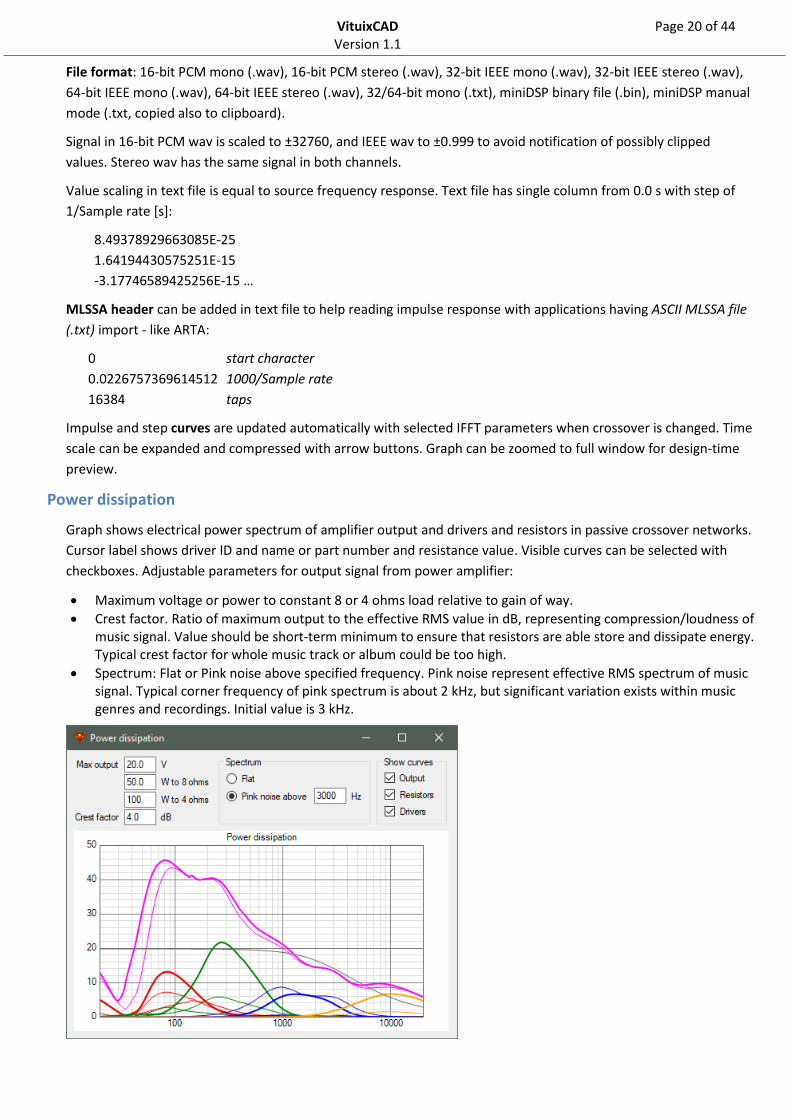
Power dissipation
Graph shows electrical power spectrum of amplifier output and drivers and resistors in passive crossover networks.
Cursor label shows driver ID and name or part number and resistance value. Visible curves can be selected with
checkboxes. Adjustable parameters for output signal from power amplifier:
Maximum voltage or power to constant 8 or 4 ohms load relative to gain of way.
Crest factor. Ratio of maximum output to the effective RMS value in dB, representing compression/loudness of music signal. Value should be short-term minimum to ensure that resistors are able store and dissipate energy. Typical crest factor for whole music track or album could be too high.
Spectrum: Flat or Pink noise above specified frequency. Pink noise represent effective RMS spectrum of music signal. Typical corner frequency of pink spectrum is about 2 kHz, but significant variation exists within music genres and recordings. Initial value is 3 kHz.
VituixCAD Page 21 of 44 Version 1.1
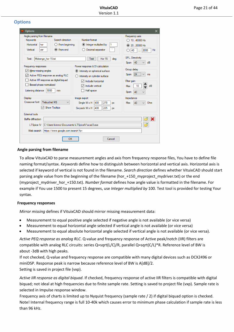
Options
Angle parsing from filename
To allow VituixCAD to parse measurement angles and axis from frequency response files, You have to define file
naming format/syntax. Keywords define how to distinguish between horizontal and vertical axis. Horizontal axis is
selected if keyword of vertical is not found in the filename. Search direction defines whether VituixCAD should start
parsing angle value from the beginning of the filename (hor_+150_myproject_mydriver.txt) or the end
(myproject_mydriver_hor_+150.txt). Number format defines how angle value is formatted in the filename. For
example if You use 1500 to present 15 degrees, use Integer multiplied by 100. Test tool is provided for testing Your
syntax.
Frequency responses
Mirror missing defines if VituixCAD should mirror missing measurement data:
Measurement to equal positive angle selected if negative angle is not available (or vice versa)
Measurement to equal horizontal angle selected if vertical angle is not available (or vice versa)
Measurement to equal absolute horizontal angle selected if vertical angle is not available (or vice versa).
Active PEQ response as analog RLC. Q-value and frequency response of Active peak/notch (IIR) filters are
compatible with analog RLC circuits: series Q=sqrt(L/C)/R, parallel Q=sqrt(C/L)*R. Reference level of BW is
about -3dB with high peaks.
If not checked, Q-value and frequency response are compatible with many digital devices such as DCX2496 or
miniDSP. Response peak is narrow because reference level of BW is A[dB]/2.
Setting is saved in project file (vxp).
Active IIR response as digital biquad. If checked, frequency response of active IIR filters is compatible with digital
biquad; not ideal at high frequencies due to finite sample rate. Setting is saved to project file (vxp). Sample rate is
selected in Impulse response window.
Frequency axis of charts is limited up to Nyquist frequency (sample rate / 2) if digital biquad option is checked.
Note! Internal frequency range is full 10-40k which causes error to minimum phase calculation if sample rate is less
than 96 kHz.
VituixCAD Page 22 of 44 Version 1.1
Bessel phase normalized. Phase angle at nominal frequency is normalized according filter order: 90° (2nd), 135° (3rd),
… 360° (8th). Level at nominal frequency varies: -4.8 dB (2nd), -6.3 dB (3rd), … -13.5 dB (8th). This is popular Bessel
function with many digital devices such as Xilica or miniDSP.
If not checked, level at nominal frequency is normalized to -3.0 dB. This is common in design tables of linear circuit
manufactures such as Analog Devices and Texas Instruments.
Before designing crossover, select Bessel response normalization which is compatible with your target system.
Setting is saved in project file (vxp).Listening distance is virtual distance from loudspeaker to listener or
microphone, needed to calculate phase differences and amplitude relations between drivers in different locations.
Enter typical listening distance in mm. Default value is 2500 mm.
Display
Font for crossover schematic and visibility of tooltips are selectable.
Power response & DI calculation
Intensity on spherical surface is normally selected for common sized single or multiway speakers. Intensity on
spherical surface around speaker is calculated from radial measurements in horizontal and vertical planes.
𝑄(𝑓) =2𝑁
𝜋∑ |𝑝(𝜃𝑛)𝑝(0)
|2
𝑁𝑛=1 𝑠𝑖𝑛𝜃𝑛
𝐷𝐼(𝑓) = 10𝑙𝑜𝑔10𝑄(𝑓)
Intensity on cylinder surface is practical selection for long line sources, or if either horizontal or vertical directivity is
temporarily interesting - not accurate power response & DI result. Intensity on cylinder surface around speaker is
calculated as average pressure from radial measurements, typically in a single (horizontal) plane.
Checkboxes control which planes are included in power response and directivity index calculations; horizontal,
vertical or both.
If Half space is checked, angles >90 deg are excluded from power response and DI calculation. Directivity chart
shows angles -90...+90 deg only. This setting is meant for flush mounted or other clearly uni-directional speakers.
Common box speakers and dipoles with DI <10 dB should be measured and simulated to full space.
Image export
Single W x H is size of exported chart image. Default size is 480x270 px.
Six-pack W x H is size of one exported chart in group of all six charts in main program or Enclosure tool. Default size
is 400x225 px.
Default size can be set by double-clicking the label.
Graph scales
Frequency axis
Internal frequency range is fixed 10…39794 Hz with density of 48 points/octave, but you can limit visible scale.
Options are fixed 20…20000 Hz or custom range with minimum 10…400 Hz and maximum 1000…40000 Hz.
SPL, Directivity
Span controls vertical scale of SPL graphs. SPL, Power & DI and Directivity waterfall span: 20, 30, 40 or 60 dB.
Group delay
Span controls vertical scale of GD & Phase graph. GD span: 2, 4, 8, 16, 24 or 40 ms.
Filter gain
Max defines upper limit and Span controls vertical scale of filter gain graph. Filter gain span: 30, 35, 40, 45, 50 or 60
dB.
VituixCAD Page 23 of 44 Version 1.1
Impedance
Max defines upper limit of impedance graph. Impedance maximum: 20, 30, 40, 60 or 80 ohm.
External tools
Paths in the text fields define applications VituixCAD should open when pressing corresponding buttons/menu
items. Select application by clicking folder button or dropping file into text box.
Baffle diffraction Executable of external diffraction simulator, for example Tolvan Edge Spice Executable of LTspice IV or compatible circuit simulator Web search Search command for drivers in Enclosure tool
Baffle diffraction text box should be empty for activating internal diffraction simulator.
VituixCAD Page 24 of 44 Version 1.1
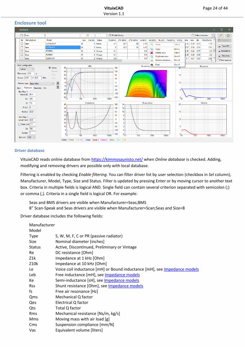
Enclosure tool
Driver database
VituixCAD reads online database from https://kimmosaunisto.net/ when Online database is checked. Adding,
modifying and removing drivers are possible only with local database.
Filtering is enabled by checking Enable filtering. You can filter driver list by user selection (checkbox in Sel column),
Manufacturer, Model, Type, Size and Status. Filter is updated by pressing Enter or by moving cursor to another text
box. Criteria in multiple fields is logical AND. Single field can contain several criterion separated with semicolon (;)
or comma (,). Criteria in a single field is logical OR. For example:
Seas and BMS drivers are visible when Manufacturer=Seas;BMS 8” Scan-Speak and Seas drivers are visible when Manufacturer=Scan;Seas and Size=8
Driver database includes the following fields:
Manufacturer Model Type S, W, M, F, C or PR (passive radiator) Size Nominal diameter [inches] Status Active, Discontinued, Preliminary or Vintage Re DC resistance [Ohm] Z1k Impedance at 1 kHz [Ohm] Z10k Impedance at 10 kHz [Ohm] Le Voice coil inductance [mH] or Bound inductance [mH], see Impedance models Leb Free inductance [mH], see Impedance models Ke Semi-inductance [sH], see Impedance models Rss Shunt resistance [Ohm], see Impedance models fs Free air resonance [Hz] Qms Mechanical Q factor Qes Electrical Q factor Qts Total Q factor Rms Mechanical resistance [Ns/m, kg/s] Mms Moving mass with air load [g] Cms Suspension compliance [mm/N] Vas Equivalent volume [liters]
VituixCAD Page 25 of 44 Version 1.1
Sd Effective cone area [cm2] Bl Force factor [N/A, Tm] Pmax Maximum long term input power [W] Xmax Maximum linear excursion, one way peak [mm] Revision Datasheet revision or date by manufacturer Updated Date/Name in format yyyy-mm-dd/First name Last name
Driver list can be sorted by clicking column header. Right click in driver row opens context menu with more options
to search and modify driver list. Context menu options:
Undo (all changes) Copy Delete rows Duplicate rows Update database Find
button searches for selected driver from web (Google search with Your default browser).
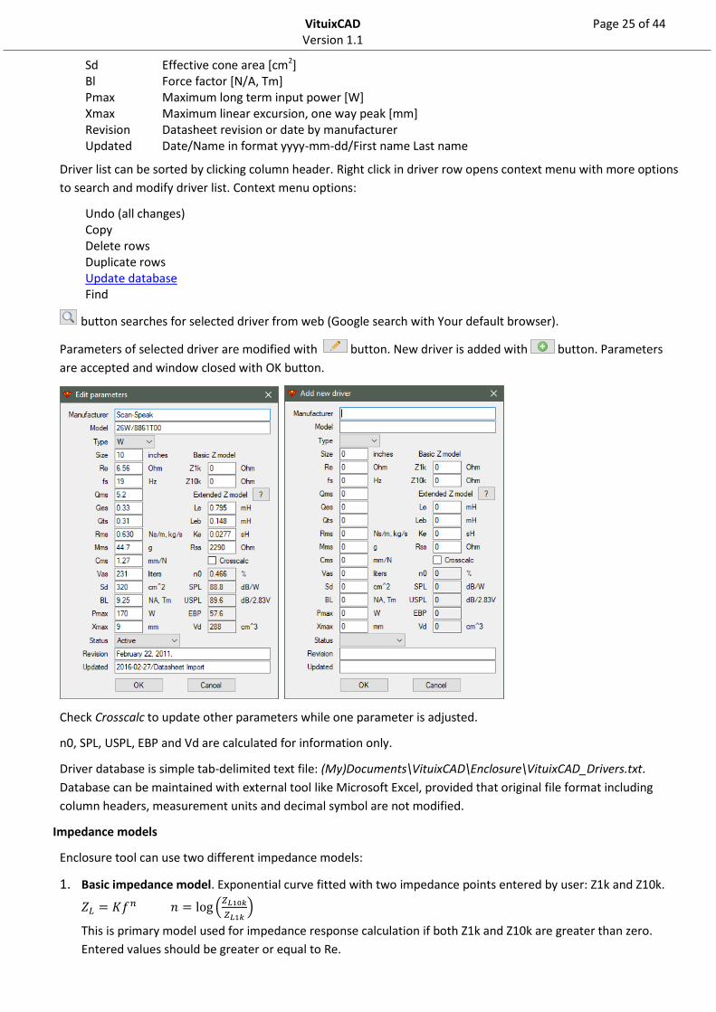
Parameters of selected driver are modified with button. New driver is added with button. Parameters
are accepted and window closed with OK button.
Check Crosscalc to update other parameters while one parameter is adjusted.
n0, SPL, USPL, EBP and Vd are calculated for information only.
Driver database is simple tab-delimited text file: (My)Documents\VituixCAD\Enclosure\VituixCAD_Drivers.txt.
Database can be maintained with external tool like Microsoft Excel, provided that original file format including
column headers, measurement units and decimal symbol are not modified.
Impedance models
Enclosure tool can use two different impedance models:
1. Basic impedance model. Exponential curve fitted with two impedance points entered by user: Z1k and Z10k.
𝑍𝐿 = 𝐾𝑓𝑛 𝑛 = log (𝑍𝐿10𝑘
𝑍𝐿1𝑘)
This is primary model used for impedance response calculation if both Z1k and Z10k are greater than zero.
Entered values should be greater or equal to Re.
VituixCAD Page 26 of 44 Version 1.1
2. Extended impedance model described in detail in the paper Frequency Dependence of Damping and
Compliance in Loudspeaker Suspensions by Knud Thorborg, Carsten Tinggaard, Finn Agerkvist and Claus
Futtrup, published in JAES Volume 58 Issue 6 pp. 472-486; June 2010.
Loudspeaker equivalent circuit (seen from electrical side):
Calculation rules if all parameters of extended impedance model are not applied:
· Semi-inductance Ke is used if bound inductance Le is blank or zero
· Bound inductance Le is used if semi-inductance Ke is blank or zero
· Shunt resistance Rss is ignored (=infinite) if blank or zero.
This is secondary model used for impedance response calculation if Z1k or Z10k or both are blank or zero.
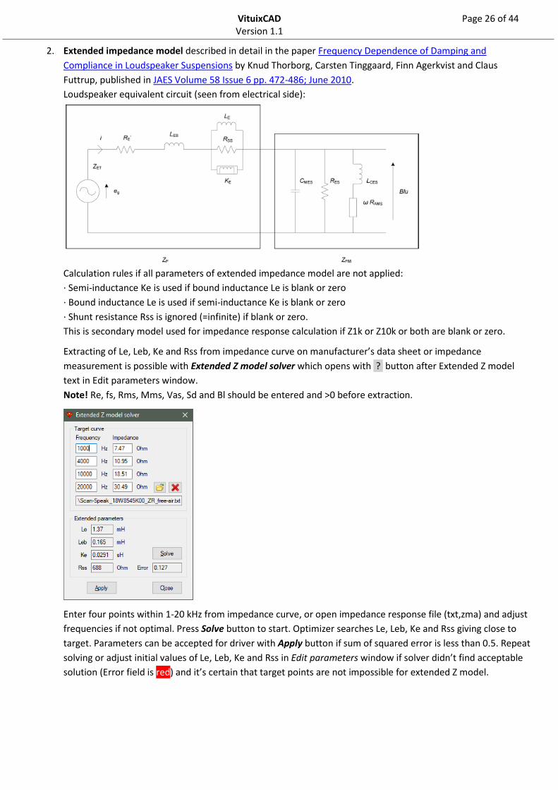
Extracting of Le, Leb, Ke and Rss from impedance curve on manufacturer’s data sheet or impedance
measurement is possible with Extended Z model solver which opens with ? button after Extended Z model
text in Edit parameters window.
Note! Re, fs, Rms, Mms, Vas, Sd and Bl should be entered and >0 before extraction.
Enter four points within 1-20 kHz from impedance curve, or open impedance response file (txt,zma) and adjust
frequencies if not optimal. Press Solve button to start. Optimizer searches Le, Leb, Ke and Rss giving close to
target. Parameters can be accepted for driver with Apply button if sum of squared error is less than 0.5. Repeat
solving or adjust initial values of Le, Leb, Ke and Rss in Edit parameters window if solver didn’t find acceptable
solution (Error field is red) and it’s certain that target points are not impossible for extended Z model.
VituixCAD Page 27 of 44 Version 1.1
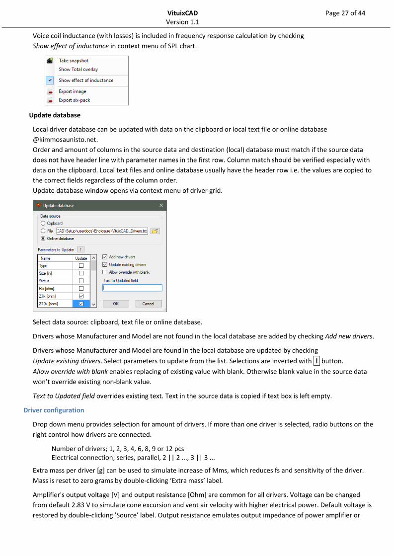
Voice coil inductance (with losses) is included in frequency response calculation by checking
Show effect of inductance in context menu of SPL chart.
Update database
Local driver database can be updated with data on the clipboard or local text file or online database
@kimmosaunisto.net.
Order and amount of columns in the source data and destination (local) database must match if the source data
does not have header line with parameter names in the first row. Column match should be verified especially with
data on the clipboard. Local text files and online database usually have the header row i.e. the values are copied to
the correct fields regardless of the column order.
Update database window opens via context menu of driver grid.
Select data source: clipboard, text file or online database.
Drivers whose Manufacturer and Model are not found in the local database are added by checking Add new drivers.
Drivers whose Manufacturer and Model are found in the local database are updated by checking
Update existing drivers. Select parameters to update from the list. Selections are inverted with ! button.
Allow override with blank enables replacing of existing value with blank. Otherwise blank value in the source data
won’t override existing non-blank value.
Text to Updated field overrides existing text. Text in the source data is copied if text box is left empty.
Driver configuration
Drop down menu provides selection for amount of drivers. If more than one driver is selected, radio buttons on the
right control how drivers are connected.
Number of drivers; 1, 2, 3, 4, 6, 8, 9 or 12 pcs Electrical connection; series, parallel, 2 || 2 ..., 3 || 3 ...
Extra mass per driver [g] can be used to simulate increase of Mms, which reduces fs and sensitivity of the driver.
Mass is reset to zero grams by double-clicking ‘Extra mass’ label.
Amplifier's output voltage [V] and output resistance [Ohm] are common for all drivers. Voltage can be changed
from default 2.83 V to simulate cone excursion and vent air velocity with higher electrical power. Default voltage is
restored by double-clicking ’Source’ label. Output resistance emulates output impedance of power amplifier or

VituixCAD Page 28 of 44 Version 1.1
cable resistance. Actual series resistance is quick and dirty way to increase electrical Q factor and decrease
sensitivity.
Radiator type
Radiator types supported by Enclosure tool:
Infinite baffle
Closed
Bass reflex
Double tuned bass reflex
Passive radiator
Band pass type 1
Band pass type 2
Band pass type 3
Tabs
Align –Closed and Bass reflex radiator alignment
Closed box is aligned by selecting or entering Qtc. Optional high alarm limit for non-linearity [% on Xmax] due to air
compression is available. Box volume is limited and requested Qtc is not produced if alarm limit is exceeded (red
text). Increase % value until red color disappears to get requested Qtc if you don’t care about compression
distortion. Box Q entered on Enclosure tab and series resistance are included in alignment by checking
Include Qb+Rs. Otherwise alignment is done by basic formula: Vb = Vas / ((Qtc/Qts)2-1). Both options are
approximations, but normally including Qb+Rs is giving results closer to effective Qtc around system resonance.
VituixCAD Page 29 of 44 Version 1.1
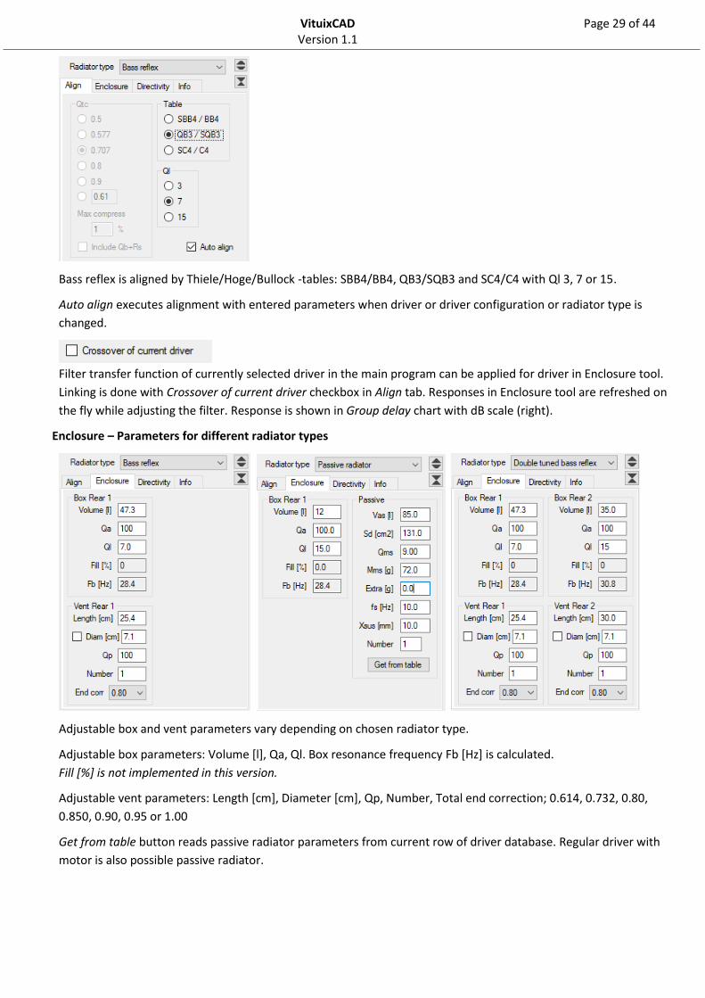
Bass reflex is aligned by Thiele/Hoge/Bullock -tables: SBB4/BB4, QB3/SQB3 and SC4/C4 with Ql 3, 7 or 15.
Auto align executes alignment with entered parameters when driver or driver configuration or radiator type is
changed.
Filter transfer function of currently selected driver in the main program can be applied for driver in Enclosure tool.
Linking is done with Crossover of current driver checkbox in Align tab. Responses in Enclosure tool are refreshed on
the fly while adjusting the filter. Response is shown in Group delay chart with dB scale (right).
Enclosure – Parameters for different radiator types
Adjustable box and vent parameters vary depending on chosen radiator type.
Adjustable box parameters: Volume [l], Qa, Ql. Box resonance frequency Fb [Hz] is calculated.
Fill [%] is not implemented in this version.
Adjustable vent parameters: Length [cm], Diameter [cm], Qp, Number, Total end correction; 0.614, 0.732, 0.80,
0.850, 0.90, 0.95 or 1.00
Get from table button reads passive radiator parameters from current row of driver database. Regular driver with
motor is also possible passive radiator.
VituixCAD Page 30 of 44 Version 1.1
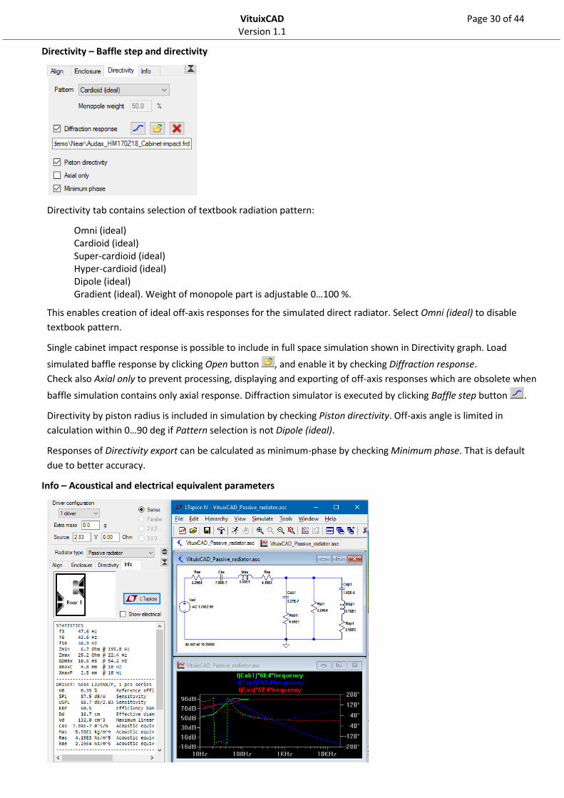
Directivity – Baffle step and directivity
Directivity tab contains selection of textbook radiation pattern:
Omni (ideal) Cardioid (ideal) Super-cardioid (ideal) Hyper-cardioid (ideal) Dipole (ideal) Gradient (ideal). Weight of monopole part is adjustable 0…100 %.
This enables creation of ideal off-axis responses for the simulated direct radiator. Select Omni (ideal) to disable
textbook pattern.
Single cabinet impact response is possible to include in full space simulation shown in Directivity graph. Load
simulated baffle response by clicking Open button , and enable it by checking Diffraction response.
Check also Axial only to prevent processing, displaying and exporting of off-axis responses which are obsolete when
baffle simulation contains only axial response. Diffraction simulator is executed by clicking Baffle step button .
Directivity by piston radius is included in simulation by checking Piston directivity. Off-axis angle is limited in
calculation within 0…90 deg if Pattern selection is not Dipole (ideal).
Responses of Directivity export can be calculated as minimum-phase by checking Minimum phase. That is default
due to better accuracy.
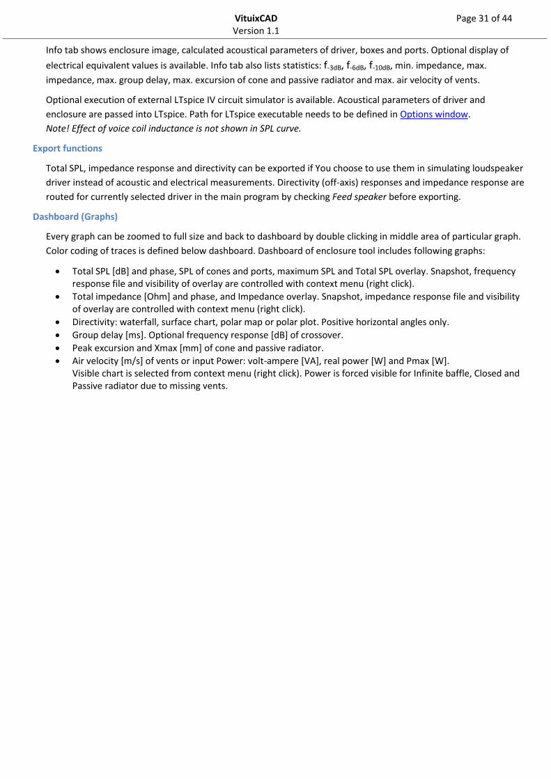
Info – Acoustical and electrical equivalent parameters
VituixCAD Page 31 of 44 Version 1.1
Info tab shows enclosure image, calculated acoustical parameters of driver, boxes and ports. Optional display of
electrical equivalent values is available. Info tab also lists statistics: f-3dB, f-6dB, f-10dB, min. impedance, max.
impedance, max. group delay, max. excursion of cone and passive radiator and max. air velocity of vents.
Optional execution of external LTspice IV circuit simulator is available. Acoustical parameters of driver and
enclosure are passed into LTspice. Path for LTspice executable needs to be defined in Options window.
Note! Effect of voice coil inductance is not shown in SPL curve.
Export functions
Total SPL, impedance response and directivity can be exported if You choose to use them in simulating loudspeaker
driver instead of acoustic and electrical measurements. Directivity (off-axis) responses and impedance response are
routed for currently selected driver in the main program by checking Feed speaker before exporting.
Dashboard (Graphs)
Every graph can be zoomed to full size and back to dashboard by double clicking in middle area of particular graph.
Color coding of traces is defined below dashboard. Dashboard of enclosure tool includes following graphs:
Total SPL [dB] and phase, SPL of cones and ports, maximum SPL and Total SPL overlay. Snapshot, frequency response file and visibility of overlay are controlled with context menu (right click).
Total impedance [Ohm] and phase, and Impedance overlay. Snapshot, impedance response file and visibility of overlay are controlled with context menu (right click).
Directivity: waterfall, surface chart, polar map or polar plot. Positive horizontal angles only.
Group delay [ms]. Optional frequency response [dB] of crossover.
Peak excursion and Xmax [mm] of cone and passive radiator.
Air velocity [m/s] of vents or input Power: volt-ampere [VA], real power [W] and Pmax [W]. Visible chart is selected from context menu (right click). Power is forced visible for Infinite baffle, Closed and Passive radiator due to missing vents.
VituixCAD Page 32 of 44 Version 1.1
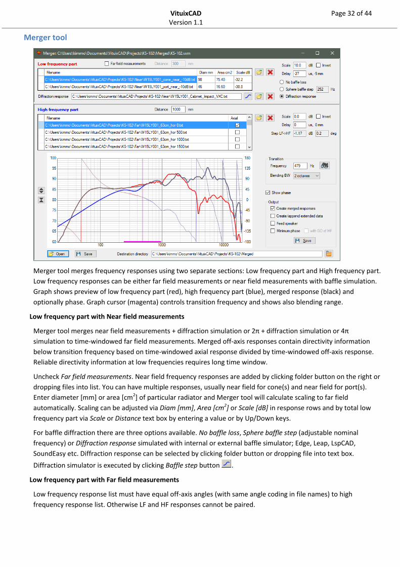
Merger tool
Merger tool merges frequency responses using two separate sections: Low frequency part and High frequency part.
Low frequency responses can be either far field measurements or near field measurements with baffle simulation.
Graph shows preview of low frequency part (red), high frequency part (blue), merged response (black) and
optionally phase. Graph cursor (magenta) controls transition frequency and shows also blending range.
Low frequency part with Near field measurements
Merger tool merges near field measurements + diffraction simulation or 2π + diffraction simulation or 4π
simulation to time-windowed far field measurements. Merged off-axis responses contain directivity information
below transition frequency based on time-windowed axial response divided by time-windowed off-axis response.
Reliable directivity information at low frequencies requires long time window.
Uncheck Far field measurements. Near field frequency responses are added by clicking folder button on the right or
dropping files into list. You can have multiple responses, usually near field for cone(s) and near field for port(s).
Enter diameter [mm] or area [cm2] of particular radiator and Merger tool will calculate scaling to far field
automatically. Scaling can be adjusted via Diam [mm], Area [cm2] or Scale [dB] in response rows and by total low
frequency part via Scale or Distance text box by entering a value or by Up/Down keys.
For baffle diffraction there are three options available. No baffle loss, Sphere baffle step (adjustable nominal
frequency) or Diffraction response simulated with internal or external baffle simulator; Edge, Leap, LspCAD,
SoundEasy etc. Diffraction response can be selected by clicking folder button or dropping file into text box.
Diffraction simulator is executed by clicking Baffle step button .
Low frequency part with Far field measurements
Low frequency response list must have equal off-axis angles (with same angle coding in file names) to high
frequency response list. Otherwise LF and HF responses cannot be paired.
VituixCAD Page 33 of 44 Version 1.1
Check Far field measurements. Far field frequency responses are added by clicking folder button on the right or
dropping files into list. Enter Distance of low frequency and high frequency measurements and Merger tool will
calculate scaling of LF responses automatically. Scaling can be adjusted via Scale text box by entering a value or by
Up/Down keys.
High frequency part
Far field measurements can be added by clicking folder button or dropping files into list. Scaling can be adjusted
manually via Scale text box on the right. Axial response is selected by checking Axial column in response file list.
Default axial response is 0 degrees in horizontal plane. Merged responses (graph below High frequency part) for
particular angle can be previewed by clicking corresponding response from file list.
Transition
Transition from low frequency to high frequency part can be set manually via Frequency text box, graph cursor or
Up/Down keys or automatically by clicking binocular button . Automatic option searches for lowest magnitude
crossing point of low and high frequency curves.
Warning is given with red background color if transition frequency exceeds maximum near field frequency of the
largest low frequency radiator. fNFmax = c/π/Dd (c = 344.0 m/s).
Magnitude and phase blending range between low and high frequency parts can be selected from drop down list:
none, 1, 2, 3 or 4 octaves.
Delay of low frequency part is calculated automatically on transition frequency change but can be adjusted
manually.
Output
Choose which items You want to output. Create merged responses will combine low frequency and high frequency
responses into individual response files. Create/append extended data will combine LF and HF responses into a
single file, having LspCAD 6 extended data format. Merged responses are routed for currently selected driver in the
main program by checking Feed speaker before saving.
Merged responses are exported as minimum-phase by checking Minimum phase. Measured and entered delays are
lost and all responses at all frequencies are normalized to the same acoustic center = 0 mm. Color of merged phase
response is lime in the chart.
Excess group delay of HF response at transition frequency x 1.4 is added to merged minimum phase response by
checking with GD of HF. This option saves measured delay (at transition frequency x 1.4) and delay adjusted by
user.
Minimum phase options may be needed if measured far field HF responses are not minimum-phase at transition
frequency, though radiator is actually minimum-phase. Significant error is possible with some measurement
programs if IR time window is short. Forcing to calculated minimum phase is not recommended if responses are
measured with dual channel gear and phase error at transition frequency is only few degrees.
Destination Directory
Choose work directory where You want to save output files.
Save and Open
Merger project can be saved with Save button in the bottom left corner. File extension is vxm, internally XML.
Saved merger project can be opened with Open button or dropping vxm-file into Merger tool window.
VituixCAD Page 34 of 44 Version 1.1
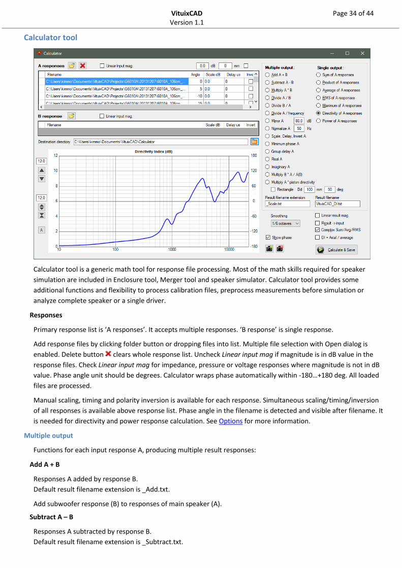
Calculator tool
Calculator tool is a generic math tool for response file processing. Most of the math skills required for speaker
simulation are included in Enclosure tool, Merger tool and speaker simulator. Calculator tool provides some
additional functions and flexibility to process calibration files, preprocess measurements before simulation or
analyze complete speaker or a single driver.
Responses
Primary response list is ‘A responses’. It accepts multiple responses. ‘B response’ is single response.
Add response files by clicking folder button or dropping files into list. Multiple file selection with Open dialog is
enabled. Delete button clears whole response list. Uncheck Linear input mag if magnitude is in dB value in the
response files. Check Linear input mag for impedance, pressure or voltage responses where magnitude is not in dB
value. Phase angle unit should be degrees. Calculator wraps phase automatically within -180…+180 deg. All loaded
files are processed.
Manual scaling, timing and polarity inversion is available for each response. Simultaneous scaling/timing/inversion
of all responses is available above response list. Phase angle in the filename is detected and visible after filename. It
is needed for directivity and power response calculation. See Options for more information.
Multiple output
Functions for each input response A, producing multiple result responses:
Add A + B
Responses A added by response B.
Default result filename extension is _Add.txt.
Add subwoofer response (B) to responses of main speaker (A).
Subtract A – B
Responses A subtracted by response B.
Default result filename extension is _Subtract.txt.
VituixCAD Page 35 of 44 Version 1.1
Multiply A * B
Responses A are multiplied by response B.
Default result filename extension is _Multiply.txt.
Create far field response by multiplying near field measurements (A) with cabinet diffraction simulation (B). Test equalizer, high pass or low pass filter by multiplying raw responses (A) with filter transfer function (B).
Divide A / B
Responses A are divided by response B.
Default result filename extension is _DivideAB.txt.
Normalize polar measurements by dividing off-axis responses (A) with axial response (B). Correct punch of uncalibrated measurements (A) by multiplying with calibration file, representing total frequency response of your measurement system (B).
Divide B / A
Response B is divided by responses A.
Default result filename extension is _DivideBA.txt.
Divide A / frequency
Responses A magnitude is divided by frequency.
Default result filename extension is _DivideByFreq.txt.
Calculate cone excursion response from near field measurement (A) by dividing each magnitude value with associate frequency.
Mirror A
Responses A mirroring aka vertical flipping over entered dB value.
Default result filename extension is _Mirror.txt.
Create equalizer target response by mirroring raw response over entered level. Create correction response by mirroring total frequency response of your measurement system.
Normalize A
Responses A normalizing to magnitude of the first response A at entered frequency.
Default result filename extension is _Normalize.txt.
Reduce excess directivity of time-windowed off-axis responses by normalizing responses at 40 Hz of axial response in case you are sure that radiator is perfect omni until 40 Hz.
Scale, Delay, Invert A
No calculation - just responses A magnitude scaling, time shifting and polarity inversion.
Default result filename extension is _Scale.txt.
Scale measurements (A) to estimated or known SPL [dB/2.83V/1m]. Smooth measurements (A) without any other manipulation. Resample measurements (A) from linear to logarithmic frequency increment; from response export of REW to 24…48 points/octave. This may require appropriate time shifting to maintain correct phase information. Time shifting of measurements (A) if time reference (0 s) point is at the mic capsule or starting point of IR time window was too much before impulse peak. Invert measurements (A) if mic polarity was inverted while measurement or your mic & preamp combination is constantly inverting.
Minimum phase A
Responses A converted to minimum-phase. Response tails below 10 Hz and above 22 kHz are estimated by the first
and last 1/2 octaves. Default result filename extension is _MinPhase.txt.
VituixCAD Page 36 of 44 Version 1.1
Group delay A
Responses A group delay in milliseconds.
Default result filename extension is _GroupDelay.txt.
Real A
Responses A converted to real: phase angle is set to 0 deg or -180 deg if Invert is checked.
Default result filename extension is _Real.txt.
Create correction file for magnitude only. Normally this corrupts minimum phase features, but may be useful if phase information is irrelevant or harmful. Create full impedance response for ideal resistive component from plain magnitude response.
Imaginary A
Responses A converted to imaginary: phase angle is set to 90 deg or -90 deg if Invert is checked.
Default result filename extension is _Imaginary.txt.
Create full impedance response for ideal reactive component from plain magnitude response.
Multiply B * A / A(0)
Creates off-axis responses for measured or captured axial response B with directivity information in responses A.
Directivity data can be simulated with Diffraction tool or compatible set of far field measurements. Response A to
0 degrees is reference in directivity calculation.
Default result filename extension is _MultiplyBdA.txt.
Multiply A * piston directivity
Responses A multiplied by piston directivity. Calculation parameters are piston diameter for circular or width for
rectangular radiator, and off-axis angle in degrees. Off-axis angle coded in filename in response list A is applied if 0
degrees is entered. Directivity function for circular radiator is 2*J1(k*a*sin(angle))/(k*a*sin(angle)), where J1(x) is
1st order Bessel function of first kind, k=wave number and a=radius. Directivity function for rectangular radiator is
Sinc(k*x*sin(angle)), where x is width. Phase shift is approximated with –k*x*sin(angle).
Default result filename extension is _PistonDir.txt.
Create off-axis response including piston directivity from single axial or near field response.
Single output
Functions for multiple input responses, producing single result response:
Sum of A responses
= A0 + A1 + A2 + …
Default result filename is VituixCAD_Sum.txt.
Create total response of multiple radiators Sum near field measurements of all cones and ports. Each response A can be scaled for different radiating area. Create total response of multiple ways/bands. Simulate comb-filtering effects by summing non-delayed and delayed responses. See Complex calculation.
Product of A responses
= A0 * A1 * A2 * …
Product calculation produces overflow error quite soon if several files is loaded. Typically product is needed for
maximum two…three responses.
Default result filename is VituixCAD_Product.txt.

VituixCAD Page 37 of 44 Version 1.1
Average of A responses
= (A0 + A1 + A2 + …) / N
Default result filename is VituixCAD_Average.txt.
Create listening window response by averaging ±30 deg hor and ±5 deg ver responses. See Complex calculation.
RMS of A responses
= SQRT((A02 + A1
2 + A22 + …) / N)
RMS is alternative for simple average (arithmetic mean). Square scales single magnitude value for area or power,
for example from sound pressure to intensity. See Complex calculation.
Default result filename is VituixCAD_RMS.txt.
Maximum of A responses
Searches maximum magnitude from responses (A) for each frequency point. Phase angle of result response is taken
from selected row.
Default result filename is VituixCAD_Maximum.txt.
Create reference response for manual Directivity Index calculation if preferred reference response is maximum pressure within listening window instead of single axial response (which could contain diffraction dips).
Directivity of A responses
Calculates Directivity Factor Q(f) from radial measurements (A) if Linear result mag is checked and DI=Axial/average is not checked. Calculates Directivity Index DI(f) from radial measurements (A) if Linear result mag and DI=Axial/average are not checked. Unit of result is dB.
Phase angle should be included in response filenames in order to calculate intensity on spherical surface from
radial measurements. Angle step must be constant.
‘Horizontal 0 deg’ response is automatically selected as directivity reference. Content of that file should be
modified in order to use some other measurement or calculated result as a reference.
Default result filename is VituixCAD_DI.txt.
Directivity can be calculated as axial to average pressure ratio by checking DI=Axial/average. This option is valid if
polar response set is real 3D containing equally spaced measurements on full spherical surface around the radiator.
Another application is to calculate either horizontal or vertical directivity, without requirement of correct result for
full space.
Power of A responses
Power response approximation is calculated as Reference response magnitude + Directivity Index + 10*log10(4π).
This method requires valid responses for Directivity Index calculation, specified in the previous section.
Default result filename is VituixCAD_Power.txt.
Additional options
Complex Sum/Avg/RMS should be checked in order to calculate complex vector sum, average or RMS with phase
angle information. Complex calculation is sensitive to phase angle; sum of two equal magnitudes with opposite
polarity = 0. This is default option giving correct results with frequency responses.
Absolute magnitudes are summed if Complex calculation is not checked. This option is useful if phase information is
too random or nonsymmetrical (like with multiple room responses) causing steep magnitude dips in result
response. Phase angle of result response is calculated with complex numbers anyway, but minimum phase features
are not completely maintained.
Smoothing options are 1/1, 1/2, 1/3, 1/6, 1/12 octaves or none.

VituixCAD Page 38 of 44 Version 1.1
Result files can be recycled to input responses by checking Result -> input. Multiple result files are recycled to
responses A, and single result file to response B. This enables calculation sequences without manual loading of
result files to input. Result files are saved in Destination directory, which can be changed via folder button.
Result files are created by clicking Calculate & Save button. Calculation to graph without result file creation is
executed when response files are loaded or calculation formula is selected or smoothing or any other additional
option is changed.
Graph
Enter title directly into graph for publishing of captured image.
Maximum and span of magnitude axis are adjusted by arrow buttons or entering value or Up/Down keys in the text
boxes. Magnitude can be auto scaled by clicking A button. Scale of phase axis is constant -180…+180 deg.
Max. 10 overlays can be added into graph with Add overlay button . Clear overlay deletes the latest visible
overlay.
VituixCAD Page 39 of 44 Version 1.1
Diffraction tool
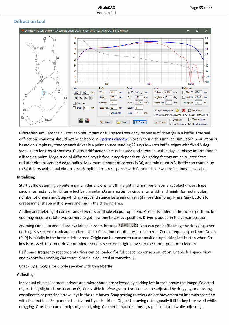
Diffraction simulator calculates cabinet impact or full space frequency response of driver(s) in a baffle. External
diffraction simulator should not be selected in Options window in order to use this internal simulator. Simulation is
based on simple ray theory: each driver is a point source sending 72 rays towards baffle edges with fixed 5 deg
steps. Path lengths of shortest 1st order diffractions are calculated and summed with delay i.e. phase information in
a listening point. Magnitude of diffracted rays is frequency dependent. Weighting factors are calculated from
radiator dimensions and edge radius. Maximum amount of corners is 36, and minimum is 3. Baffle can contain up
to 50 drivers with equal dimensions. Simplified room response with floor and side wall reflections is available.
Initializing
Start baffle designing by entering main dimensions; width, height and number of corners. Select driver shape;
circular or rectangular. Enter effective diameter Dd or area Sd for circular or width and height for rectangular,
number of drivers and Step which is vertical distance between drivers (if more than one). Press New button to
create initial shape with drivers and mic in the drawing area.
Adding and deleting of corners and drivers is available via pop-up menu. Corner is added in the cursor position, but
you may need to rotate two corners to get new one to correct position. Driver is added in the cursor position.
Zooming Out, 1, In and Fit are available via zoom buttons . You can pan baffle image by dragging when
nothing is selected (blank area clicked). Unit of location coordinates is millimeter. Zoom 1 equals 1px=1mm. Origin
(0, 0) is initially in the bottom left corner. Origin can be moved to cursor position by clicking left button when Ctrl
key is pressed. If corner, driver or microphone is selected, origin moves to the center point of selection.
Half space frequency response of driver can be loaded for full space response simulation. Enable full space view
and export by checking Full space. Y-scale is adjusted automatically.
Check Open baffle for dipole speaker with thin I-baffle.
Adjusting
Individual objects; corners, drivers and microphone are selected by clicking left button above the image. Selected
object is highlighted and location (X, Y) is visible in View group. Location can be adjusted by dragging or entering
coordinates or pressing arrow keys in the text boxes. Snap setting restricts object movement to intervals specified
with the text box. Snap mode is activated by a checkbox. Object is moving orthogonally if Shift key is pressed while
dragging. Crosshair cursor helps object aligning. Cabinet impact response graph is updated while adjusting.

VituixCAD Page 40 of 44 Version 1.1
Remove selection (deselect) by clicking blank area. Coordinates of mouse cursor are shown as long as nothing is
selected.
Edge radius and Driver Dd or Sd, Width and Height can be adjusted after project initialization by entering value or
pressing up/down keys in the text boxes. Drawing and cabinet impact response graph are updated while adjusting.
Mic/listening point
Microphone symbol represents listening point at Axis Distance. Baffle can be rotated horizontally and vertically by
entering Axis Angle Hor or Ver, or pressing up/down keys in the text boxes. Rotation origin is perpendicular point of
microphone on (unrotated) baffle surface.
Reflections
Check Floor and enter floor elevation in mm to include floor bounce in frequency response. Side wall reflection is
included by checking Wall. Negative X coordinate locates wall on the left side. Enter absorption within 0…20 dB to
reduce amplitude of boundary reflections.
File functions
Save baffle project by pressing Save button. File extension is .vxb, but it’s human-readable xml file containing main
dimensions and location of corners and drivers. You can print the file for helping final enclosure design.
Open existing baffle project by pressing Open button.
Export simulated Cabinet impact response or full space frequency response shown in the graph by pressing Export
button.
You can also export off-axis responses with 10 deg steps by checking Directivity. Responses in vertical plane
10…170 deg are exported by checking Vertical plane. Responses to negative angles -10…-170 deg are exported by
checking Negative angles. Responses are routed for currently selected driver in the main program by checking
Feed speaker before exporting. Enter root file name for responses. Program extends file name with
horizontal/vertical keyword and angle, using coding defined in Options window.
Graph
Max. 10 overlays can be added into response graph with Add overlay button . Clear overlay deletes the
latest visible overlay.
Note!
1) Bevel can be entered as radius.
2) Long planar radiator should be constructed by stacking multiple small rectangular drivers with Step = Height.
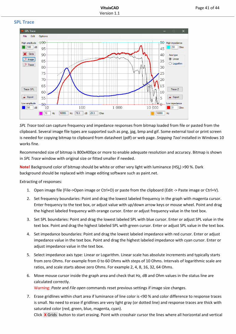
VituixCAD Page 41 of 44 Version 1.1
SPL Trace
SPL Trace tool can capture frequency and impedance responses from bitmap loaded from file or pasted from the
clipboard. Several image file types are supported such as png, jpg, bmp and gif. Some external tool or print screen
is needed for copying bitmap to clipboard from datasheet (pdf) or web page. Snipping Tool installed in Windows 10
works fine.
Recommended size of bitmap is 800x400px or more to enable adequate resolution and accuracy. Bitmap is shown
in SPL Trace window with original size or fitted smaller if needed.
Note! Background color of bitmap should be white or other very light with luminance (HSL) >90 %. Dark
background should be replaced with image editing software such as paint.net.
Extracting of responses:
1. Open image file (File->Open image or Ctrl+O) or paste from the clipboard (Edit -> Paste image or Ctrl+V).
2. Set frequency boundaries: Point and drag the lowest labeled frequency in the graph with magenta cursor.
Enter frequency to the text box, or adjust value with up/down arrow keys or mouse wheel. Point and drag
the highest labeled frequency with orange cursor. Enter or adjust frequency value in the text box.
3. Set SPL boundaries: Point and drag the lowest labeled SPL with blue cursor. Enter or adjust SPL value in the
text box. Point and drag the highest labeled SPL with green cursor. Enter or adjust SPL value in the text box.
4. Set impedance boundaries: Point and drag the lowest labeled impedance with red cursor. Enter or adjust
impedance value in the text box. Point and drag the highest labeled impedance with cyan cursor. Enter or
adjust impedance value in the text box.
5. Select impedance axis type: Linear or Logarithm. Linear scale has absolute increments and typically starts
from zero Ohms. For example from 0 to 60 Ohms with steps of 10 Ohms. Intervals of logarithmic scale are
ratios, and scale starts above zero Ohms. For example 2, 4, 8, 16, 32, 64 Ohms.
6. Move mouse cursor inside the graph area and check that Hz, dB and Ohm values in the status line are
calculated correctly.
Warning: Paste and File open commands reset previous settings if image size changes.
7. Erase gridlines within chart area if luminance of line color is <90 % and color difference to response traces
is small. No need to erase if gridlines are very light gray (or dotted line) and response traces are thick with
saturated color (red, green, blue, magenta, cyan).
Click X Grids button to start erasing. Point with crosshair cursor the lines where all horizontal and vertical
VituixCAD Page 42 of 44 Version 1.1
gridlines are found, but the cursor lines crosses response traces as little as possible. Accept with left click.
Gridlines (with luminance <90 %) should be gone.
8. You can use Image rubber for cleaning vicinity of response curves. Crossing off-axis responses could
interfere tracing of axial and impedance responses.
Warning! Do not cut axial or impedance responses too much because Undo is not available.
9. Trace amplitude response. Click Trace SPL button and then starting point of frequency response at the
lowest visible frequency. Click again few pixels further if tracing was not started. Traced path is marked
with thick red overlay line. If the tracing is interrupted or distracted in an intersection, you can correct the
path by clicking a point few pixels after the problem. You can also restart from earlier position or beginning
as many times you like.
10. You can use Trace rubber for cleaning bad points of traced curve. For example short jumps above or below
correct path. Erased parts will be interpolated when the response is exported to a file.
Check Options -> Smooth 1/12 oct. to remove small peaks and tiny steps due to pixels of original bitmap.
Smoothing of 1/12 oct. is applied to exported responses.
Default density of export is 48 points/octave. Lower densities are available in Options menu, but not
recommended if responses are created for VituixCAD.
11. Export amplitude response with Export button after tracing is completed and red overlay line looks fine.
Enter filename and select extension (txt or frd). Phase response is calculated automatically as minimum
phase. Program estimates slopes of frequency response extensions below and above visible range.
12. Trace impedance response. Click Trace Z button and then starting point of impedance response at the
lowest visible frequency. And so on…
13. Export impedance response with Export button…
Traced sound pressure points can be copied to clipboard with Edit -> Copy raw SPL. Traced impedance points can be
copied to clipboard with Edit -> Copy raw Z. Phase angle is zero and decimal symbol defined in Control panel.
Press Shift key while moving mouse above the image to open circular Magnifier of 400 %.
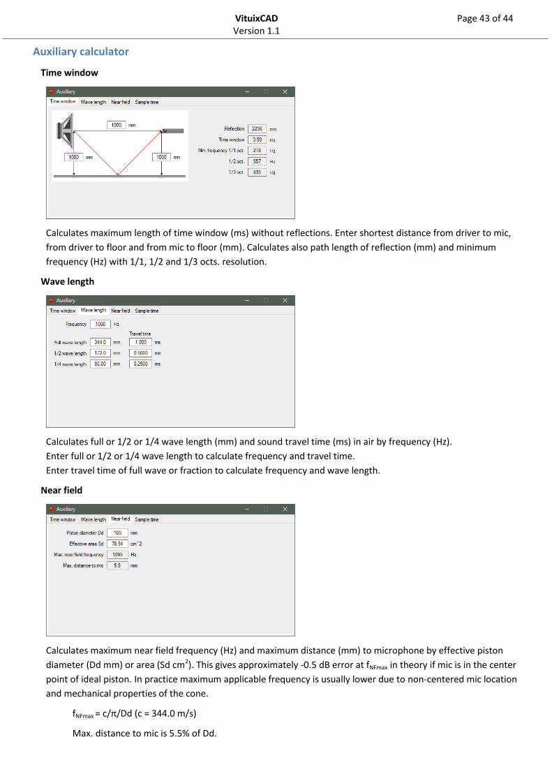
VituixCAD Page 43 of 44 Version 1.1
Auxiliary calculator
Time window
Calculates maximum length of time window (ms) without reflections. Enter shortest distance from driver to mic,
from driver to floor and from mic to floor (mm). Calculates also path length of reflection (mm) and minimum
frequency (Hz) with 1/1, 1/2 and 1/3 octs. resolution.
Wave length
Calculates full or 1/2 or 1/4 wave length (mm) and sound travel time (ms) in air by frequency (Hz).
Enter full or 1/2 or 1/4 wave length to calculate frequency and travel time.
Enter travel time of full wave or fraction to calculate frequency and wave length.
Near field
Calculates maximum near field frequency (Hz) and maximum distance (mm) to microphone by effective piston
diameter (Dd mm) or area (Sd cm2). This gives approximately -0.5 dB error at fNFmax in theory if mic is in the center
point of ideal piston. In practice maximum applicable frequency is usually lower due to non-centered mic location
and mechanical properties of the cone.
fNFmax = c/π/Dd (c = 344.0 m/s)
Max. distance to mic is 5.5% of Dd.
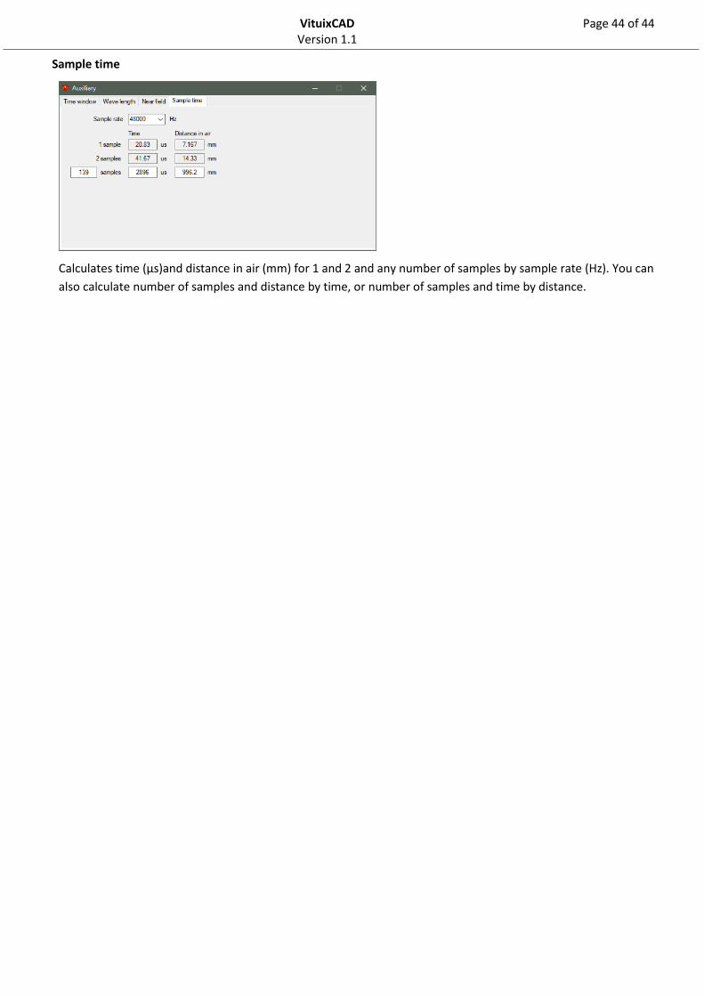
VituixCAD Page 44 of 44 Version 1.1
Sample time
Calculates time (µs)and distance in air (mm) for 1 and 2 and any number of samples by sample rate (Hz). You can
also calculate number of samples and distance by time, or number of samples and time by distance.


![[Kestävän aluesuunnittelun työkalut käyttöön 3.10.2013]: Kimmo Lylykangas, Arkkitehtuuritoimisto Kimmo Lylykangas: Ilmastotavoitteita toteuttava asemakaavoitus -raportin tulokset](https://static.fdocuments.net/doc/165x107/54717587b4af9fa90a8b4b69/kestaevaen-aluesuunnittelun-tyoekalut-kaeyttoeoen-3102013-kimmo-lylykangas-arkkitehtuuritoimisto-kimmo-lylykangas-ilmastotavoitteita-toteuttava-asemakaavoitus-raportin-tulokset.jpg)