Virtual Work 3rd Year Structural Engineering 2008/9colincaprani.com/files/notes/SAIII/Virtual Work...
118
Structural Analysis III Virtual Work 3rd Year Structural Engineering 2008/9 Dr. Colin Caprani Dr. C. Caprani 1
Transcript of Virtual Work 3rd Year Structural Engineering 2008/9colincaprani.com/files/notes/SAIII/Virtual Work...
Structural Analysis III
Virtual Work
3rd Year
Structural Engineering
2008/9
Dr. Colin Caprani
Dr. C. Caprani 1

Structural Analysis III
Contents 1. Introduction ......................................................................................................... 4
1.1 General............................................................................................................. 4
1.2 Background...................................................................................................... 5
2. The Principle of Virtual Work......................................................................... 14
2.1 Definition....................................................................................................... 14
2.2 Virtual Displacements ................................................................................... 15
2.3 Virtual Forces ................................................................................................ 16
2.4 Simple Proof using Virtual Displacements ................................................... 17
2.5 Internal and External Virtual Work............................................................... 18
3. Application of Virtual Displacements ............................................................. 20
3.1 Rigid Bodies .................................................................................................. 20
3.2 Deformable Bodies ........................................................................................ 27
3.3 Problems ........................................................................................................ 37
4. Application of Virtual Forces........................................................................... 39
4.1 Basis............................................................................................................... 39
4.2 Deflection of Trusses..................................................................................... 40
4.3 Deflection of Beams and Frames .................................................................. 47
4.4 Integration of Bending Moments................................................................... 53
4.5 Problems ........................................................................................................ 56
5. Virtual Work for Indeterminate Structures................................................... 62
5.1 General Approach.......................................................................................... 62
5.2 Using Virtual Work to Find the Multiplier ................................................... 64
5.3 Indeterminate Trusses.................................................................................... 66
5.4 Indeterminate Frames .................................................................................... 70
5.5 Continuous Beams......................................................................................... 76
5.6 Problems ........................................................................................................ 84
6. Virtual Work for Self-Stressed Structures ..................................................... 87
Dr. C. Caprani 2

Structural Analysis III
6.1 Background.................................................................................................... 87
6.2 Trusses ........................................................................................................... 93
6.3 Beams ............................................................................................................ 99
6.4 Frames.......................................................................................................... 101
6.5 Problems ...................................................................................................... 106
7. Past Exam Questions....................................................................................... 108
7.1 Summer 1997............................................................................................... 108
7.2 Summer 1998............................................................................................... 109
7.3 Summer 1999............................................................................................... 110
7.4 Summer 2000............................................................................................... 111
7.5 Summer 2001............................................................................................... 112
7.6 Summer 2002............................................................................................... 113
7.7 Summer 2004............................................................................................... 114
7.8 Summer 2007............................................................................................... 115
7.9 Semester 2, 2008.......................................................................................... 116
8. References ........................................................................................................ 117
9. Appendix – Volume Integrals......................................................................... 118
Dr. C. Caprani 3
Structural Analysis III
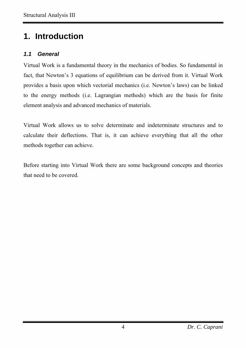
1. Introduction
1.1 General
Virtual Work is a fundamental theory in the mechanics of bodies. So fundamental in
fact, that Newton’s 3 equations of equilibrium can be derived from it. Virtual Work
provides a basis upon which vectorial mechanics (i.e. Newton’s laws) can be linked
to the energy methods (i.e. Lagrangian methods) which are the basis for finite
element analysis and advanced mechanics of materials.
Virtual Work allows us to solve determinate and indeterminate structures and to
calculate their deflections. That is, it can achieve everything that all the other
methods together can achieve.
Before starting into Virtual Work there are some background concepts and theories
that need to be covered.
Dr. C. Caprani 4

Structural Analysis III
1.2 Background
Strain Energy and Work Done
Strain energy is the amount of energy stored in a structural member due to
deformation caused by an external load. For example, consider this simple spring:
We can see that as it is loaded by a gradually increasing force, F, it elongates. We can
graph this as:
The line OA does not have to be straight, that is, the constitutive law of the spring’s
material does not have to be linear.
Dr. C. Caprani 5
Structural Analysis III
An increase in the force of a small amount, Fδ results in a small increase in
deflection, yδ . The work done during this movement (force × displacement) is the
average force during the course of the movement, times the displacement undergone.
This is the same as the hatched trapezoidal area above. Thus, the increase in work
associated with this movement is:
( )2
2
F F FU y
F yF y
F y
δδ δ
δ δδ
δ
+ += ⋅
⋅= ⋅ +
≈ ⋅
(1.1)
where we can neglect second-order quantities. As 0yδ → , we get:
dU F dy= ⋅
The total work done when a load is gradually applied from 0 up to a force of F is the
summation of all such small increases in work, i.e.:
0
yU F d= y∫ (1.2)
This is the dotted area underneath the load-deflection curve of earlier and represents
the work done during the elongation of the spring. This work (or energy, as they are
the same thing) is stored in the spring and is called strain energy and denoted U.
If the load-displacement curve is that of a linearly-elastic material then where
k is the constant of proportionality (or the spring stiffness). In this case, the dotted
area under the load-deflection curve is a triangle.
F ky=
Dr. C. Caprani 6
Structural Analysis III
Draw this:
Dr. C. Caprani 7
Structural Analysis III
As we know that the work done is the area under this curve, then the work done by
the load in moving through the displacement – the External Work Done, - is given
by:
eW
12eW F= y (1.3)
We can also calculate the strain energy, or Internal Work Done, , by: IW
0
0
212
y
y
U F d
ky dy
ky
=
=
=
∫∫
y
Also, since , we then have: F ky=
( )1 12 2IW U ky y F= = = y
I
But this is the external work done, . Hence we have: eW
eW W= (1.4)
Which we may have expected from the Law of Conservation of Energy. Thus:
The external work done by external forces moving through external displacements is
equal to the strain energy stored in the material.
Dr. C. Caprani 8
Structural Analysis III
Law of Conservation of Energy
For structural analysis this can be stated as:
Consider a structural system that is isolated such it neither gives nor receives
energy; the total energy of this system remains constant.
The isolation of the structure is key: we can consider a structure isolated once we
have identified and accounted for all sources of restraint and loading. For example, to
neglect the self-weight of a beam is problematic as the beam receives gravitational
energy not accounted for, possibly leading to collapse.
In the spring and force example, we have accounted for all restraints and loading (for
example we have ignored gravity by having no mass). Thus the total potential energy
of the system, Π , is constant both before and after the deformation.
In structural analysis the relevant forms of energy are the potential energy of the load
and the strain energy of the material. We usually ignore heat and other energies.
Potential Energy of the Load
Since after the deformation the spring has gained strain energy, the load must have
lost potential energy, V. Hence, after deformation we have for the total potential
energy:
212
U V
ky Fy
Π = +
= − (1.5)
In which the negative sign indicates a loss of potential energy for the load.
Dr. C. Caprani 9
Structural Analysis III
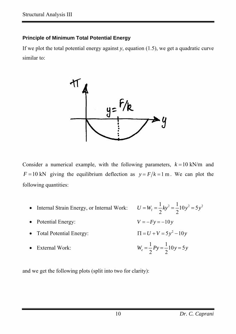
Principle of Minimum Total Potential Energy
If we plot the total potential energy against y, equation (1.5), we get a quadratic curve
similar to:
Consider a numerical example, with the following parameters, and
giving the equilibrium deflection as
10 kN/mk =
10 kNF = 1 my F k= = . We can plot the
following quantities:
• Internal Strain Energy, or Internal Work: 2 21 110 52 2IU W ky y y= = = = 2
y
• Potential Energy: 10V Fy= − = −
• Total Potential Energy: 25 10U V y yΠ = + = −
• External Work: 1 110 52 2eW Py y y= = =
and we get the following plots (split into two for clarity):
Dr. C. Caprani 10

Structural Analysis III
-10
-5
0
5
10
15
20
25
30
35
-0.5 0.0 0.5 1.0 1.5 2.0 2.5
Deflection, y
Ene
rgy
Total Potential EnergyExternal WorkInternal WorkEquilibrium
-40
-30
-20
-10
0
10
20
30
40
-0.5 0.0 0.5 1.0 1.5 2.0 2.5
Deflection, y
Ene
rgy
Total Potential EnergyStrain EnergyPotential EnergyEquilibrium
From these graphs we can see that because increases quadratically with y, while
the increases only linearly,
IW
eW IW always catches up with , and there will always
be a non-zero equilibrium point where
eW
e IW W= .
Dr. C. Caprani 11
Structural Analysis III
Admittedly, these plots are mathematical: the deflection of the spring will not take up
any value; it takes that value which achieves equilibrium. At this point we consider a
small variation in the total potential energy of the system. Considering F and k to be
constant, we can only alter y. The effect of this small variation in y is:
( ) ( ) ( ) ( )
( ) ( )
( ) ( )
2 2
2
2
1 12 21 122 2
12
y y y k y y F y y ky F
k y y F y k y
ky F y k y
δ δ δ
δ δ δ
δ δ
Π + −Π = + − + − +
= ⋅ − ⋅ +
= − +
y
(1.6)
Similarly to a first derivate, for to be an extreme (either maximum or minimum),
the first variation must vanish:
Π
( ) ( )1 0ky F yδ δΠ = − = (1.7)
Therefore:
0ky F− = (1.8)
Which we recognize to be the 0xF =∑ . Thus equilibrium occurs when is an
extreme.
Π
Before introducing more complicating maths, an example of the above variation in
equilibrium position is the following. Think of a shopkeeper testing an old type of
scales for balance – she slightly lifts one side, and if it returns to position, and no
large rotations occur, she concludes the scales is in balance. She has imposed a
Dr. C. Caprani 12
Structural Analysis III
variation in displacement, and finds that since no further displacement occurs, the
‘structure’ was originally in equilibrium.
Examining the second variation (similar to a second derivate):
( ) ( )22 1 02
k yδ δΠ = ≥ (1.9)
We can see it is always positive and hence the extreme found was a minimum. This is
a particular proof of the general principle that structures take up deformations that
minimize the total potential energy to achieve equilibrium. In short, nature is lazy!
To summarize our findings:
• Every isolated structure has a total potential energy;
• Equilibrium occurs when structures can minimise this energy;
• A small variation of the total potential energy vanishes when the structure is in
equilibrium.
These concepts are brought together in the Principle of Virtual Work.
Dr. C. Caprani 13
Structural Analysis III
2. The Principle of Virtual Work
2.1 Definition
Based upon the Principle of Minimum Total Potential Energy, we can see that any
small variation about equilibrium must do no work. Thus, the Principle of Virtual
Work states that:
A body is in equilibrium if, and only if, the virtual work of all forces acting on
the body is zero.
In this context, the word ‘virtual’ means ‘having the effect of, but not the actual form
of, what is specified’. Thus we can imagine ways in which to impose virtual work,
without worrying about how it might be achieved in the physical world.
Virtual Work
There are two ways to define virtual work, as follows.
1. Principle of Virtual Displacements:
Virtual work is the work done by the actual forces acting on the body moving
through a virtual displacement.
2. Principle of Virtual Forces:
Virtual work is the work done by a virtual force acting on the body moving
through the actual displacements.
Dr. C. Caprani 14
Structural Analysis III
2.2 Virtual Displacements
A virtual displacement is a displacement that is only imagined to occur. This is
exactly what we did when we considered the vanishing of the first variation of Π ; we
found equilibrium. Thus the application of a virtual displacement is a means to find
this first variation of Π .
So given any real force, F, acting on a body to which we apply a virtual
displacement. If the virtual displacement at the location of and in the direction of F is
yδ , then the force F does virtual work W F yδ δ= ⋅ .
There are requirements on what is permissible as a virtual displacement. For
example, in the simple proof of the Principle of Virtual Work (to follow) it can be
seen that it is assumed that the directions of the forces applied to P remain
unchanged. Thus:
• virtual displacements must be small enough such that the force directions are
maintained.
The other very important requirement is that of compatibility:
• virtual displacements within a body must be geometrically compatible with
the original structure. That is, geometrical constraints (i.e. supports) and
member continuity must be maintained.
In summary, virtual displacements are not real, they can be physically impossible but
they must be compatible with the geometry of the original structure and they must be
small enough so that the original geometry is not significantly altered.
As the deflections usually encountered in structures do not change the overall
geometry of the structure, this requirement does not cause problems.
Dr. C. Caprani 15
Structural Analysis III
2.3 Virtual Forces
So far we have only considered small virtual displacements and real forces. The
virtual displacements are arbitrary: they have no relation to the forces in the system,
or its actual deformations. Therefore virtual work applies to any set of forces in
equilibrium and to any set of compatible displacements and we are not restricted to
considering only real force systems and virtual displacements. Hence, we can use a
virtual force system and real displacements. Obviously, in structural design it is these
real displacements that are of interest and so virtual forces are used often.
A virtual force is a force imagined to be applied and is then moved through the actual
deformations of the body, thus causing virtual work.
So if at a particular location of a structure, we have a deflection, y, and impose a
virtual force at the same location and in the same direction of Fδ we then have the
virtual work W y Fδ δ= ⋅ .
Virtual forces must form an equilibrium set of their own. For example, if a virtual
force is applied to the end of a spring there will be virtual stresses in the spring as
well as a virtual reaction.
Dr. C. Caprani 16

Structural Analysis III
2.4 Simple Proof using Virtual Displacements
We can prove the Principle of Virtual Work quite simply, as follows. Consider a
particle P under the influence of a number of forces which have a resultant
force,
1, , nF K F
RF . Apply a virtual displacement of yδ to P, moving it to P’, as shown:
The virtual work done by each of the forces is:
1 1 n n RW F y F y F yRδ δ δ= ⋅ + + ⋅ = ⋅K δ
Where 1yδ is the virtual displacement along the line of action of and so on. Now
if the particle P is in equilibrium, then the forces have no resultant. That is,
there is no net force. Hence we have:
1F
1, , nF K F
0n
1 10 R nW y F y F yδ δ δ δ= ⋅ = ⋅ + + ⋅ =K (2.1)
Proving that when a particle is in equilibrium the virtual work of all the forces acting
on it sum to zero. Conversely, a particle is only in equilibrium if the virtual work
done during a virtual displacement is zero.
Dr. C. Caprani 17

Structural Analysis III
2.5 Internal and External Virtual Work
Consider the spring we started with, as shown again below. Firstly it is unloaded.
Then a load, F, is applied, causing a deflection y. It is now in its equilibrium position
and we apply a virtual displacement, yδ to the end of the spring, as shown:
A free body diagram of the end of the spring is:
Thus the virtual work done by the two forces acting on the end of the spring is:
W F y ky yδ δ δ= ⋅ − ⋅
If the spring is to be in equilibrium we must then have:
00
WF y ky y
F y kyF ky
y
δδ δ
δ δ
=⋅ − ⋅ =
⋅ = ⋅=
Dr. C. Caprani 18
Structural Analysis III
That is, the force in the spring must equal the applied force, as we already know.
However, if we define the following:
• External virtual work, EW F yδ δ= ⋅ ;
• Internal virtual work, IW ky yδ δ= ⋅ ;
We then have:
00I E
WW W
δδ δ
=− =
Thus:
EW WIδ δ= (2.2)
which states that the external virtual work must equal the internal virtual work for a
structure to be in equilibrium.
It is in this form that the Principle of Virtual Work finds most use.
Of significance also in the equating of internal and external virtual work, is that there
are no requirements for the material to have any particular behaviour. That is, virtual
work applies to all bodies, whether linearly-elastic, elastic, elasto-plastic, plastic etc.
Thus the principle has more general application than most other methods of analysis.
Internal and external virtual work can arise from either virtual displacements or
virtual forces.
Dr. C. Caprani 19
Structural Analysis III
3. Application of Virtual Displacements
3.1 Rigid Bodies
Basis
Rigid bodies do not deform and so there is no internal virtual work done. Thus:
0
0E I
i i
WW W
F y
δδ δ
δ
==
⋅ =∑ (3.1)
A simple application is to find the reactions of statically determinate structures.
However, to do so, we need to make use of the following principle:
Principle of Substitution of Constraints
Having to keep the constraints in place is a limitation of virtual work. However, we
can substitute the restraining force (i.e. the reaction) in place of the restraint itself.
That is, we are turning a geometric constraint into a force constraint. This is the
Principle of Substitution of Constraints. We can use this principle to calculate
unknown reactions:
1. Replace the reaction with its appropriate force in the same direction (or sense);
2. Impose a virtual displacement on the structure;
3. Calculate the reaction, knowing 0Wδ = .
Dr. C. Caprani 20
Structural Analysis III
Reactions of Determinate and Indeterminate Structures
For statically determinate structures, removing a restraint will always render a
mechanism (or rigid body) and so the reactions of statically determinate structures are
easily obtained using virtual work. For indeterminate structures, removing a restraint
does not leave a mechanism and hence the virtual displacements are harder to
establish since the body is not rigid.
Dr. C. Caprani 21
Structural Analysis III
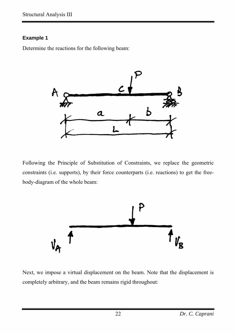
Example 1
Determine the reactions for the following beam:
Following the Principle of Substitution of Constraints, we replace the geometric
constraints (i.e. supports), by their force counterparts (i.e. reactions) to get the free-
body-diagram of the whole beam:
Next, we impose a virtual displacement on the beam. Note that the displacement is
completely arbitrary, and the beam remains rigid throughout:
Dr. C. Caprani 22
Structural Analysis III
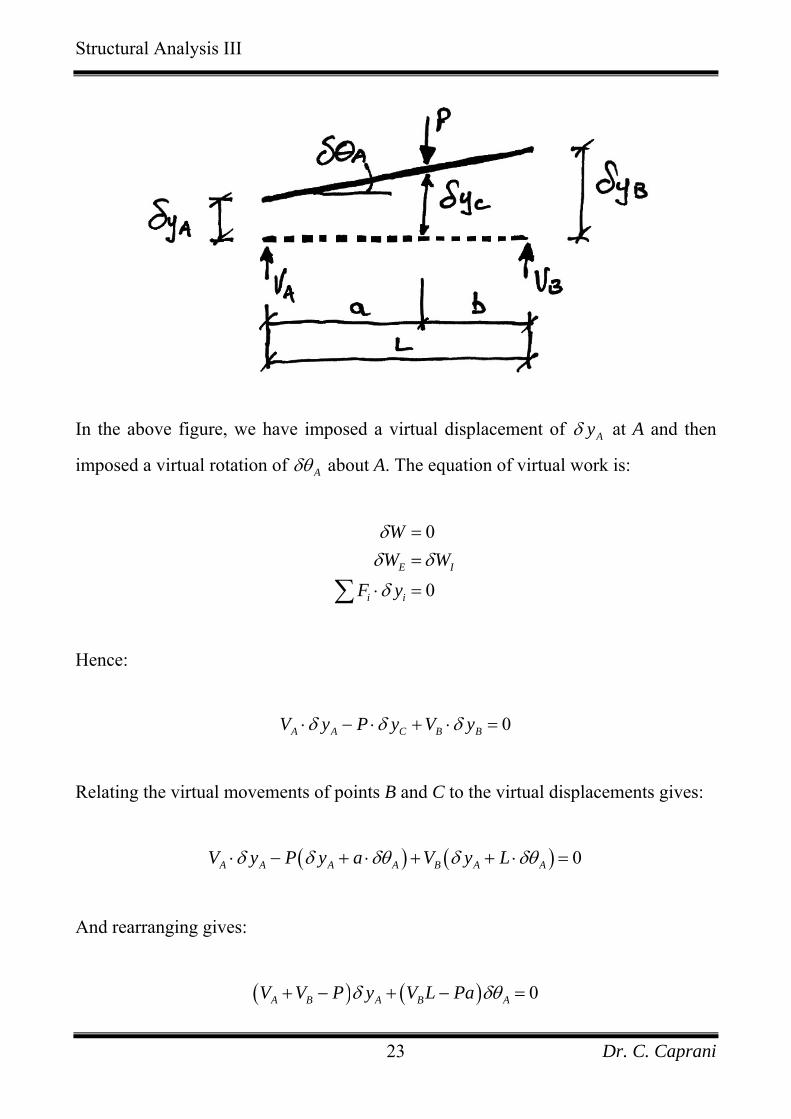
In the above figure, we have imposed a virtual displacement of Ayδ at A and then
imposed a virtual rotation of Aδθ about A. The equation of virtual work is:
0
0E I
i i
WW W
F y
δδ δ
δ
==
⋅ =∑
Hence:
0A A C B BV y P y V yδ δ δ⋅ − ⋅ + ⋅ =
Relating the virtual movements of points B and C to the virtual displacements gives:
( ) ( ) 0A A A A B A AV y P y a V y Lδ δ δθ δ δθ⋅ − + ⋅ + + ⋅ =
And rearranging gives:
( ) ( ) 0A B A B AV V P y V L Paδ δθ+ − + − =
Dr. C. Caprani 23
Structural Analysis III
And here is the power of virtual work: since we are free to choose any value we want
for the virtual displacements (i.e. they are completely arbitrary), we can choose
0Aδθ = and 0Ayδ = , which gives the following two equations:
( ) 00
A B A
A B
V V P yV V P
δ+ − =
+ − =
( ) 00
B A
B
V L PaV L Pa
δθ− =
− =
But the first equation is just 0yF =∑ whilst the second is the same as
. Thus equilibrium equations occur naturally within the virtual work
framework. Note also that the two choices made for the virtual displacements
correspond to the following virtual displaced configurations: Draw them
about 0M A =∑
Dr. C. Caprani 24
Structural Analysis III
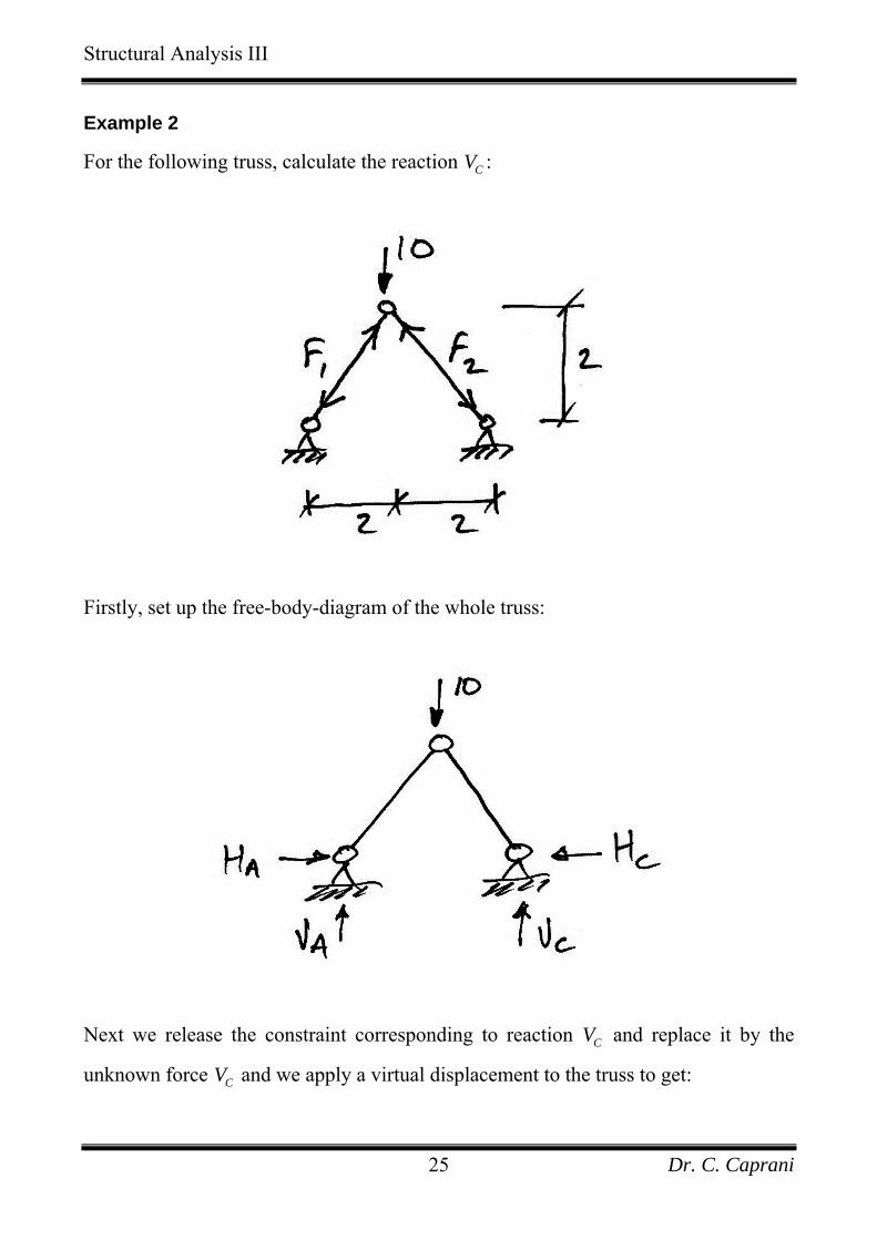
Example 2
For the following truss, calculate the reaction : CV
Firstly, set up the free-body-diagram of the whole truss:
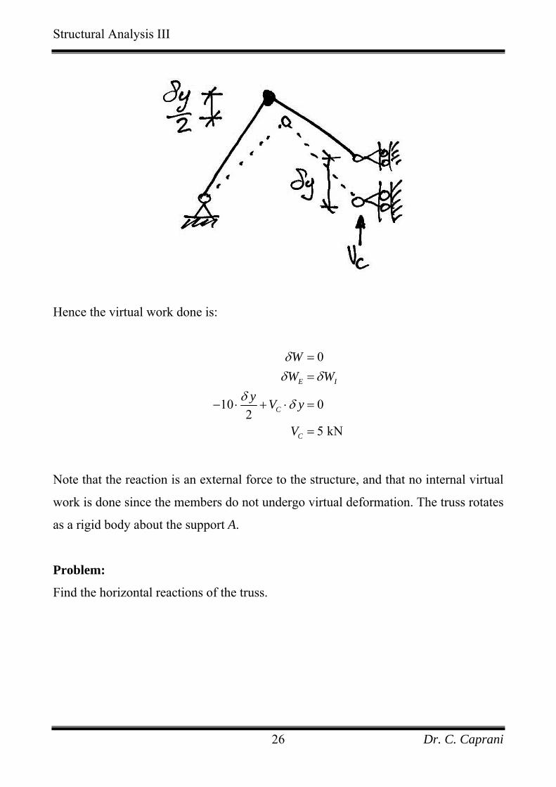
Next we release the constraint corresponding to reaction and replace it by the
unknown force and we apply a virtual displacement to the truss to get:
CV
CV
Dr. C. Caprani 25
Structural Analysis III
Hence the virtual work done is:
0
10 02
5 kN
E I
C
C
WW W
y V y
V
δδ δ
δ δ
==
− ⋅ + ⋅ =
=
Note that the reaction is an external force to the structure, and that no internal virtual
work is done since the members do not undergo virtual deformation. The truss rotates
as a rigid body about the support A.
Problem:
Find the horizontal reactions of the truss.
Dr. C. Caprani 26
Structural Analysis III
3.2 Deformable Bodies
Basis
For a virtual displacement we have:
0
E I
i i i
WW W
F y P ei
δδ δ
δ δ
==
⋅ = ⋅∑ ∫
In which, for the external virtual work, represents an externally applied force (or
moment) and
iF
iyδ its virtual displacement. And for the internal virtual work,
represents the internal force in member i and
iP
ieδ its virtual deformation. Different
stress resultants have different forms of internal work, and we will examine these.
Lastly, the summations reflect the fact that all work done must be accounted for.
Remember in the above, each the displacements must be compatible and the forces
must be in equilibrium, summarized as:
Set of forces in
equilibrium
i i i iF y P eδ δ⋅ = ⋅∑ ∑
Set of compatible
displacements
Dr. C. Caprani 27
Structural Analysis III
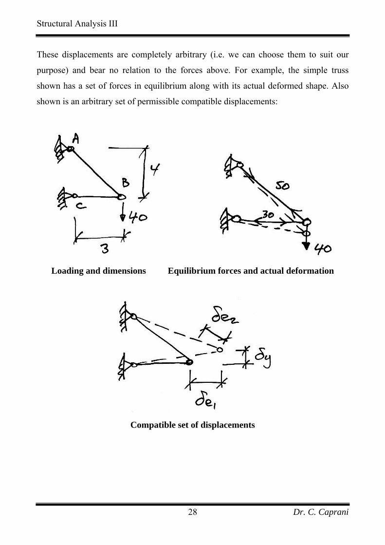
These displacements are completely arbitrary (i.e. we can choose them to suit our
purpose) and bear no relation to the forces above. For example, the simple truss
shown has a set of forces in equilibrium along with its actual deformed shape. Also
shown is an arbitrary set of permissible compatible displacements:
Loading and dimensions Equilibrium forces and actual deformation
Compatible set of displacements
Dr. C. Caprani 28

Structural Analysis III
Internal Virtual Work by Axial Force
Members subject to axial force may have the following:
• real force by a virtual displacement:
IW P eδ δ= ⋅
• virtual force by a real displacement:
IW e Pδ δ= ⋅
We have avoided integrals over the length of the member since we will only consider
prismatic members.
Dr. C. Caprani 29
Structural Analysis III
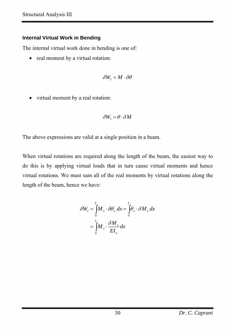
Internal Virtual Work in Bending
The internal virtual work done in bending is one of:
• real moment by a virtual rotation:
IW Mδ δθ= ⋅
• virtual moment by a real rotation:
IW Mδ θ δ= ⋅
The above expressions are valid at a single position in a beam.
When virtual rotations are required along the length of the beam, the easiest way to
do this is by applying virtual loads that in turn cause virtual moments and hence
virtual rotations. We must sum all of the real moments by virtual rotations along the
length of the beam, hence we have:
0 0
0
L L
I x x x x
Lx
xx
W M dx M d
MM dxEI
δ δθ θ δ
δ
= ⋅ = ⋅
= ⋅
∫ ∫
∫
x
Dr. C. Caprani 30
Structural Analysis III
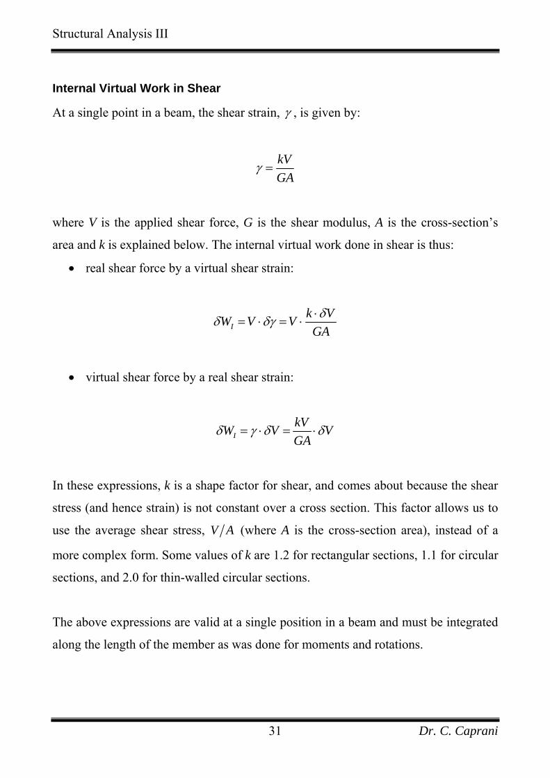
Internal Virtual Work in Shear
At a single point in a beam, the shear strain, γ , is given by:
kVGA
γ =
where V is the applied shear force, G is the shear modulus, A is the cross-section’s
area and k is explained below. The internal virtual work done in shear is thus:
• real shear force by a virtual shear strain:
Ik VW V VGAδδ δγ ⋅
= ⋅ = ⋅
• virtual shear force by a real shear strain:
IkVW VGA
Vδ γ δ δ= ⋅ = ⋅
In these expressions, k is a shape factor for shear, and comes about because the shear
stress (and hence strain) is not constant over a cross section. This factor allows us to
use the average shear stress, V A (where A is the cross-section area), instead of a
more complex form. Some values of k are 1.2 for rectangular sections, 1.1 for circular
sections, and 2.0 for thin-walled circular sections.
The above expressions are valid at a single position in a beam and must be integrated
along the length of the member as was done for moments and rotations.
Dr. C. Caprani 31
Structural Analysis III
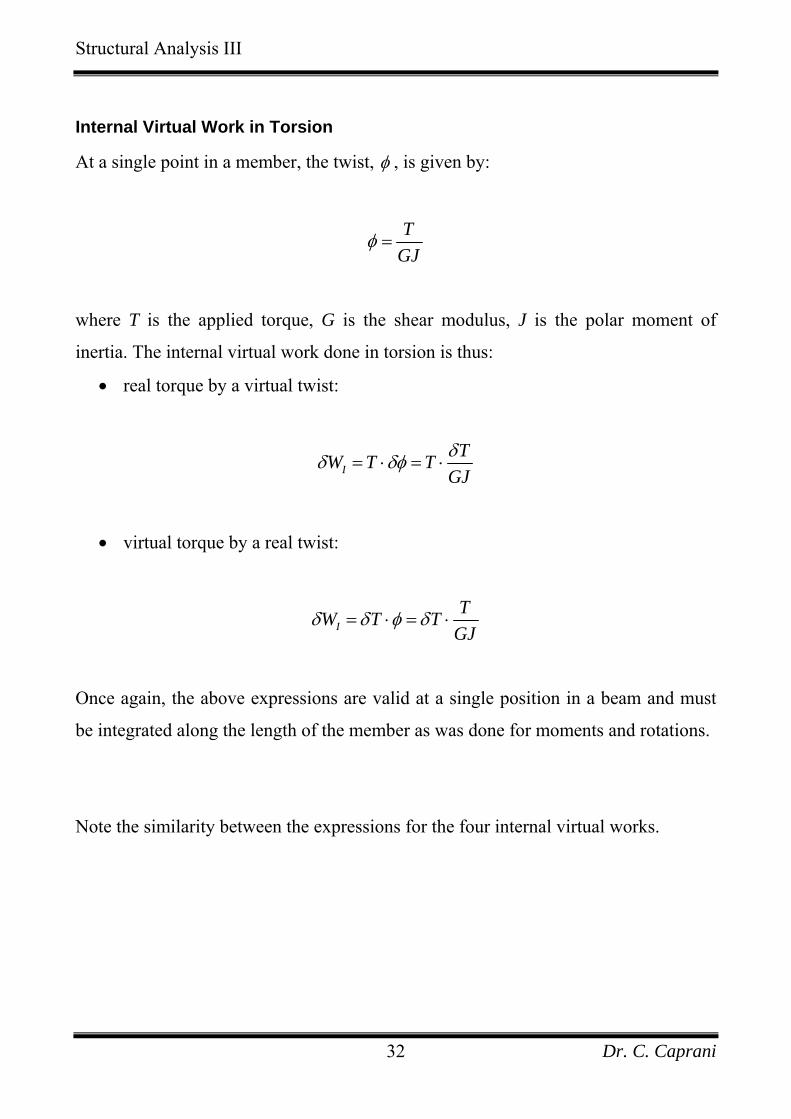
Internal Virtual Work in Torsion
At a single point in a member, the twist, φ , is given by:
TGJ
φ =
where T is the applied torque, G is the shear modulus, J is the polar moment of
inertia. The internal virtual work done in torsion is thus:
• real torque by a virtual twist:
ITW T T
GJδδ δφ= ⋅ = ⋅
• virtual torque by a real twist:
ITW T T
GJδ δ φ δ= ⋅ = ⋅
Once again, the above expressions are valid at a single position in a beam and must
be integrated along the length of the member as was done for moments and rotations.
Note the similarity between the expressions for the four internal virtual works.
Dr. C. Caprani 32
Structural Analysis III
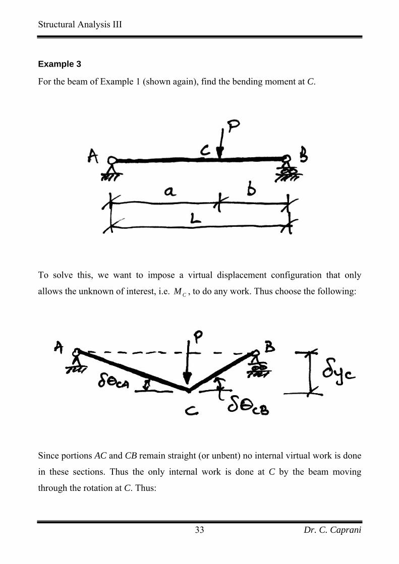
Example 3
For the beam of Example 1 (shown again), find the bending moment at C.
To solve this, we want to impose a virtual displacement configuration that only
allows the unknown of interest, i.e. CM , to do any work. Thus choose the following:
Since portions AC and CB remain straight (or unbent) no internal virtual work is done
in these sections. Thus the only internal work is done at C by the beam moving
through the rotation at C. Thus:
Dr. C. Caprani 33
Structural Analysis III
0
E I
C C
WW W
P y M C
δδ δδ δθ
==
⋅ = ⋅
Bu the rotation at C is made up as:
C CA C
C C
C
y ya ba b yab
Bδθ δθ δθδ δ
δ
= +
= +
+⎛ ⎞= ⎜ ⎟⎝ ⎠
But , hence: a b L+ =
C C
C
LP y M yab
PabM
C
L
δ δ⎛ ⎞⋅ = ⋅ ⎜ ⎟⎝ ⎠
=
We can verify this from the reactions found previously: ( )C BM V b Pa L b= ⋅ = .
Dr. C. Caprani 34
Structural Analysis III
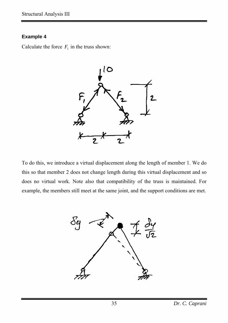
Example 4
Calculate the force in the truss shown: 1F
To do this, we introduce a virtual displacement along the length of member 1. We do
this so that member 2 does not change length during this virtual displacement and so
does no virtual work. Note also that compatibility of the truss is maintained. For
example, the members still meet at the same joint, and the support conditions are met.
Dr. C. Caprani 35

Structural Analysis III
The virtual work done is then:
1
1
0
102
10 5 2 kN2
E I
WW W
y F y
F
δδ δδ δ
==
− ⋅ = − ⋅
= =
Note some points on the signs used:
1. Negative external work is done because the 10 kN load moves upwards; i.e. the
reverse direction to its action.
2. We assumed member 1 to be in compression but then applied a virtual
elongation to the member thus reducing its internal virtual work. Hence
negative internal work is done.
3. We initially assumed to be in compression and we obtained a positive
answer confirming our assumption.
1F
Problem:
Investigate the vertical and horizontal equilibrium of the loaded joint by considering
vertical and horizontal virtual displacements separately.
Dr. C. Caprani 36
Structural Analysis III
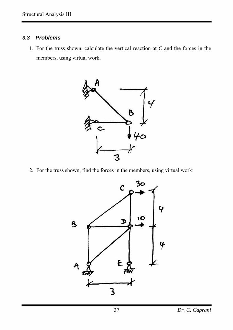
3.3 Problems
1. For the truss shown, calculate the vertical reaction at C and the forces in the
members, using virtual work.
2. For the truss shown, find the forces in the members, using virtual work:
Dr. C. Caprani 37
Structural Analysis III
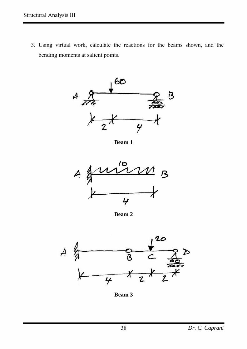
3. Using virtual work, calculate the reactions for the beams shown, and the
bending moments at salient points.
Beam 1
Beam 2
Beam 3
Dr. C. Caprani 38
Structural Analysis III
4. Application of Virtual Forces
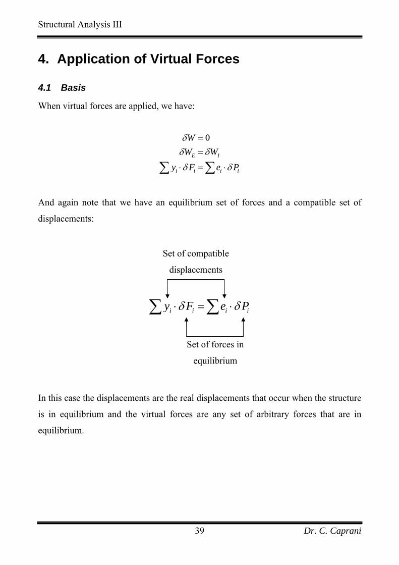
4.1 Basis
When virtual forces are applied, we have:
0
E I
i i i
WW W
y F e Pi
δδ δ
δ δ
==
⋅ = ⋅∑ ∑
And again note that we have an equilibrium set of forces and a compatible set of
displacements:
Set of compatible
displacements
i i i iy F e Pδ δ⋅ = ⋅∑ ∑
Set of forces in
equilibrium
In this case the displacements are the real displacements that occur when the structure
is in equilibrium and the virtual forces are any set of arbitrary forces that are in
equilibrium.
Dr. C. Caprani 39
Structural Analysis III
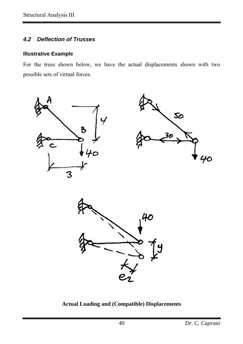
4.2 Deflection of Trusses
Illustrative Example
For the truss shown below, we have the actual displacements shown with two
possible sets of virtual forces.
Actual Loading and (Compatible) Displacements
Dr. C. Caprani 40

Structural Analysis III
Virtual Force (Equilibrium) Systems
In this truss, we know we know:
1. The forces in the members (got from virtual displacements or statics);
2. Thus we can calculate the member extensions, as: ie
ii
PLeEA
⎛ ⎞= ⎜ ⎟⎝ ⎠
3. Also, as we can choose what our virtual force Fδ is (usually unity), we have:
0
E I
i i i i
ii
WW W
y F e P
PLy F PEA
δδ δ
δ δ
δ δ
==
⋅ = ⋅
⎛ ⎞⋅ = ⋅⎜ ⎟⎝ ⎠
∑ ∑
∑
4. Since in this equation, y is the only unknown, we can calculate the deflection
of the truss.
Dr. C. Caprani 41
Structural Analysis III
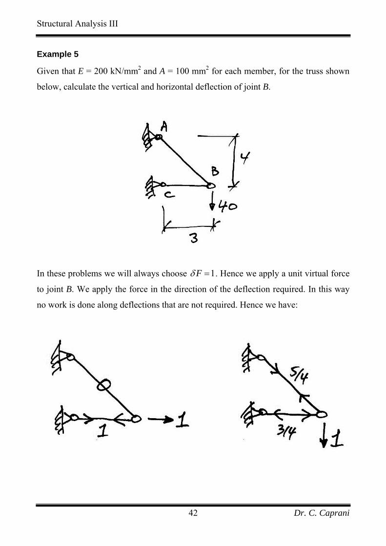
Example 5
Given that E = 200 kN/mm2 and A = 100 mm2 for each member, for the truss shown
below, calculate the vertical and horizontal deflection of joint B.
In these problems we will always choose 1Fδ = . Hence we apply a unit virtual force
to joint B. We apply the force in the direction of the deflection required. In this way
no work is done along deflections that are not required. Hence we have:
Dr. C. Caprani 42
Structural Analysis III
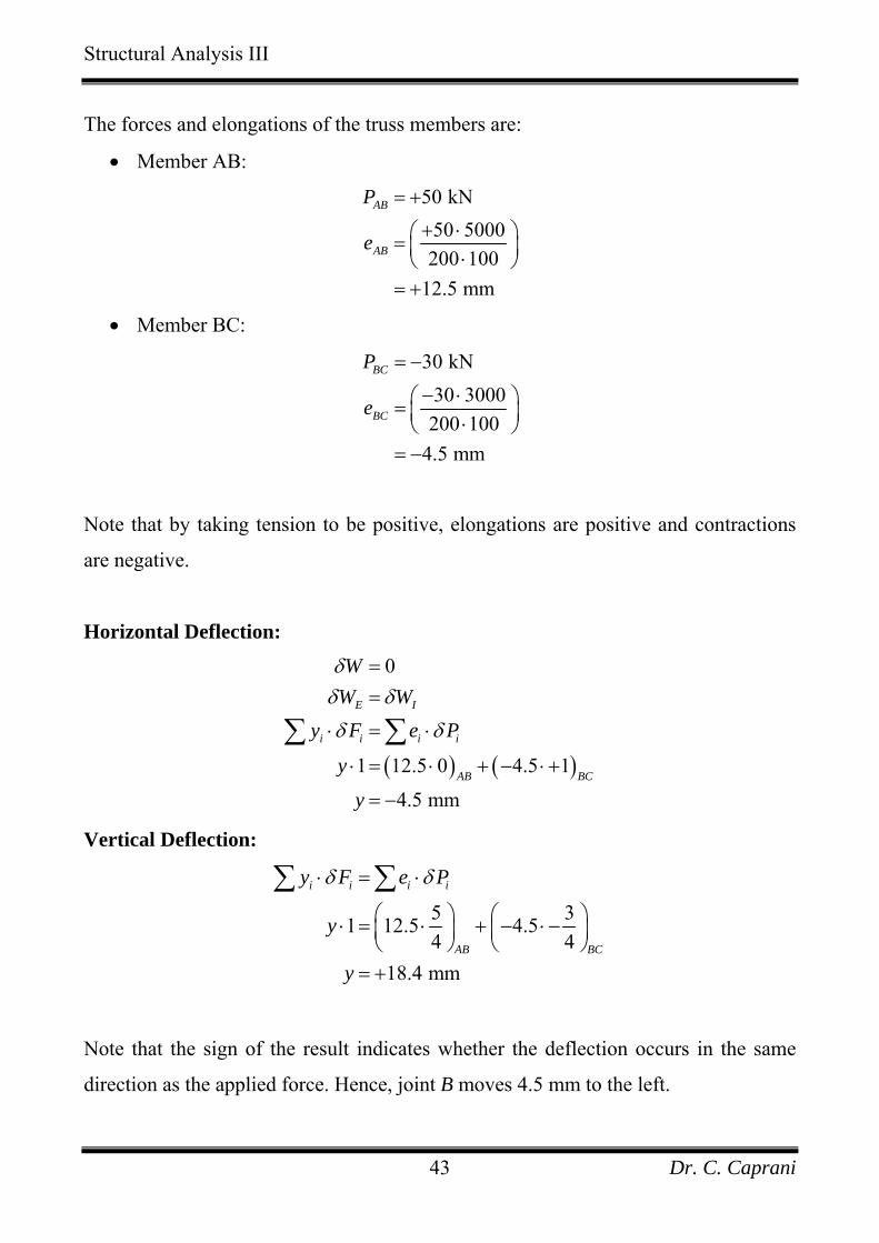
The forces and elongations of the truss members are:
• Member AB:
50 kN50 5000200 100
12.5 mm
AB
AB
P
e
= +
+ ⋅⎛ ⎞= ⎜ ⎟⋅⎝ ⎠= +
• Member BC:
30 kN30 3000200 100
4.5 mm
BC
BC
P
e
= −
− ⋅⎛ ⎞= ⎜ ⎟⋅⎝ ⎠= −
Note that by taking tension to be positive, elongations are positive and contractions
are negative.
Horizontal Deflection:
( ) ( )
0
1 12.5 0 4.5 1
4.5 mm
E I
i i i i
AB B
WW W
y F e P
y
yC
δδ δ
δ δ
==
⋅ = ⋅
⋅ = ⋅ + − ⋅ +
= −
∑ ∑
Vertical Deflection:
5 31 12.5 4.54 4
18.4 mm
i i i i
AB B
y F e P
y
y
δ δ⋅ = ⋅
⎛ ⎞ ⎛⋅ = ⋅ + − ⋅ −⎜ ⎟ ⎜⎝ ⎠ ⎝
= +
∑ ∑
C
⎞⎟⎠
Note that the sign of the result indicates whether the deflection occurs in the same
direction as the applied force. Hence, joint B moves 4.5 mm to the left.
Dr. C. Caprani 43
Structural Analysis III
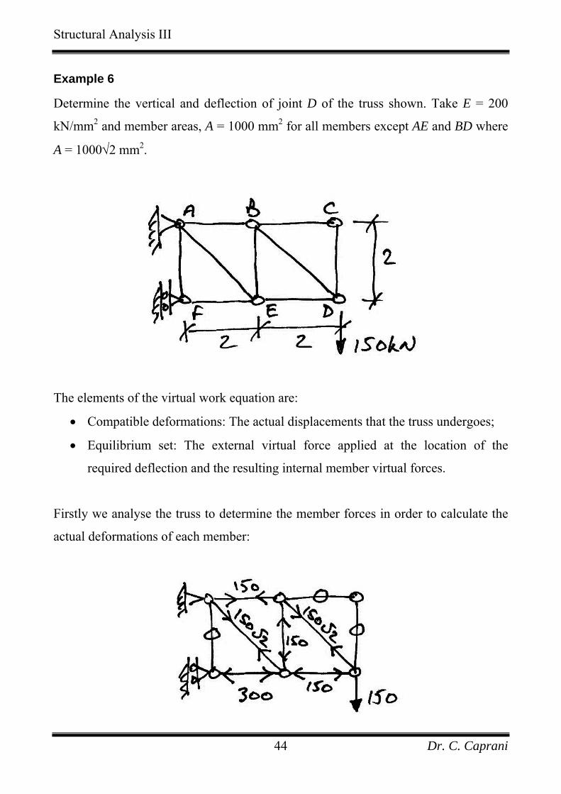
Example 6
Determine the vertical and deflection of joint D of the truss shown. Take E = 200
kN/mm2 and member areas, A = 1000 mm2 for all members except AE and BD where
A = 1000√2 mm2.
The elements of the virtual work equation are:
• Compatible deformations: The actual displacements that the truss undergoes;
• Equilibrium set: The external virtual force applied at the location of the
required deflection and the resulting internal member virtual forces.
Firstly we analyse the truss to determine the member forces in order to calculate the
actual deformations of each member:
Dr. C. Caprani 44
Structural Analysis III
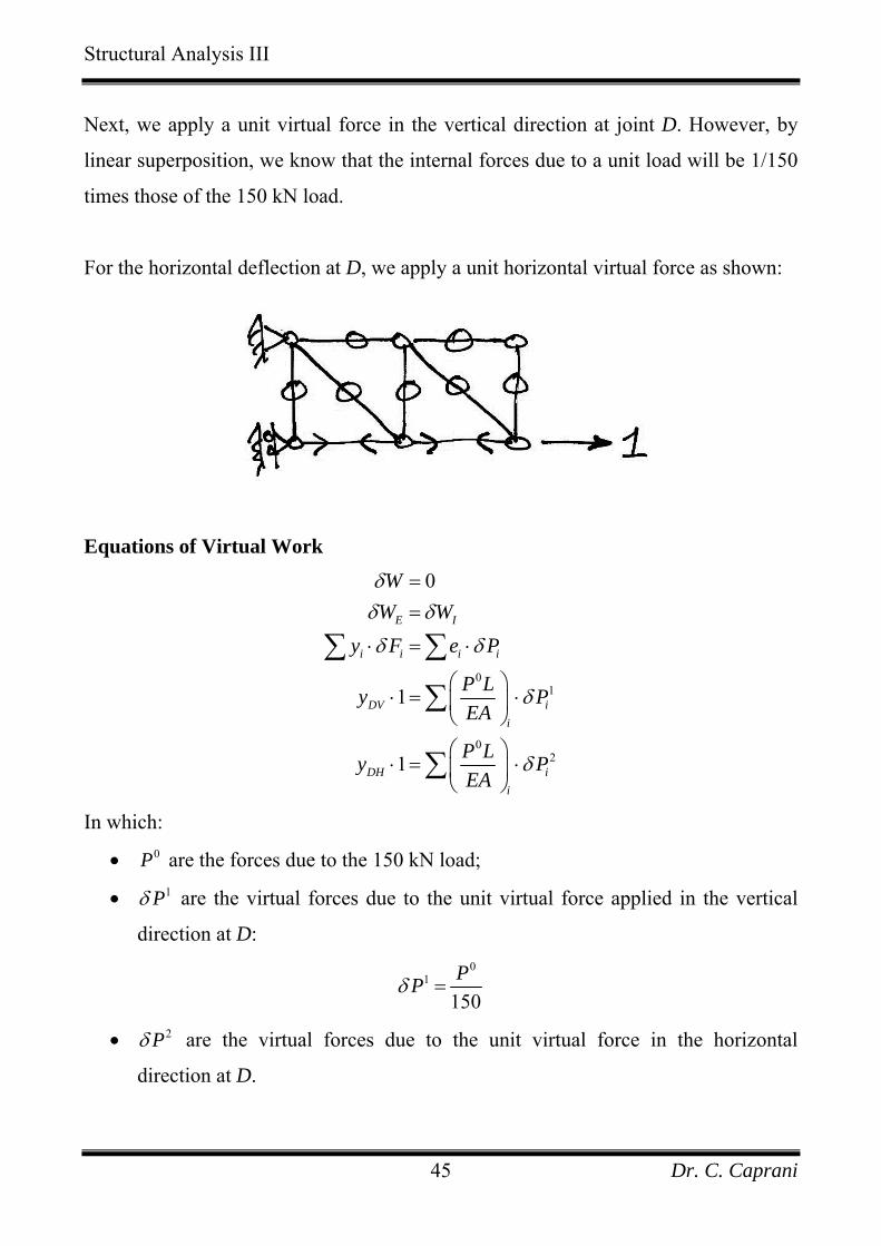
Next, we apply a unit virtual force in the vertical direction at joint D. However, by
linear superposition, we know that the internal forces due to a unit load will be 1/150
times those of the 150 kN load.
For the horizontal deflection at D, we apply a unit horizontal virtual force as shown:
Equations of Virtual Work
01
02
0
1
1
E I
i i i i
DV ii
DH ii
WW W
y F e P
P Ly PEA
P Ly PEA
δδ δ
δ δ
δ
δ
==
⋅ = ⋅
⎛ ⎞⋅ = ⋅⎜ ⎟
⎝ ⎠
⎛ ⎞⋅ = ⋅⎜ ⎟
⎝ ⎠
∑ ∑
∑
∑
In which:
• 0P are the forces due to the 150 kN load;
• 1Pδ are the virtual forces due to the unit virtual force applied in the vertical
direction at D:
0
1
150PPδ =
• 2Pδ are the virtual forces due to the unit virtual force in the horizontal
direction at D.
Dr. C. Caprani 45

Structural Analysis III
Using a table is easiest because of the larger number of members:
L A 0P 0
1
150PPδ = 2Pδ
01P L P
Aδ
⎛ ⎞⋅⎜ ⎟
⎝ ⎠
02P L P
Aδ
⎛ ⎞⋅⎜ ⎟
⎝ ⎠Member
(mm) (mm2) (kN) (kN) (kN) (kN/mm)×kN (kN/mm)×kNAB
AE
AF
BC
BD
BE
CD
DE
EF
2000
2000√2
2000
2000
2000√2
2000
2000
2000
2000
1000
1000√2
1000
1000
1000√2
1000
1000
1000
1000
+150
+150√2
0
0
+150√2
-150
0
-150
-300
+1
+1√2
0
0
+1√2
-1
0
-1
-2
0
0
0
0
0
0
0
+1
+1
+300
+600
0
0
+600
+300
0
+300
+1200
0
0
0
0
0
0
0
-300
-600
=∑ 3300 -900
E is left out because it is common. Returning to the equations, we now have: 0
111
3300 16.5 mm200
DV ii
DV
P Ly PE A
y
δ⎛ ⎞
⋅ = ⋅⎜ ⎟⎝ ⎠
+= = +
∑
Which indicates a downwards deflection and for the horizontal deflection: 0
211
900 4.5 mm200
DH ii
DH
P Ly PE A
y
δ⎛ ⎞
⋅ = ⋅⎜ ⎟⎝ ⎠
−= = −
∑
The sign indicates that it is deflecting to the left.
Dr. C. Caprani 46

Structural Analysis III
4.3 Deflection of Beams and Frames
Example 7
Using virtual work, calculate the deflection at the centre of the beam shown, given
that EI is constant.
To calculate the deflection at C, we will be using virtual forces. Therefore the two
relevant sets are:
• Compatibility set: the actual deflection at C and the rotations that occur along
the length of the beam;
• Equilibrium set: a unit virtual force applied at C which is in equilibrium with
the internal virtual moments it causes.
Compatibility Set:
The external deflection at C is what is of interest to us. To calculate the rotations
along the length of the beam we have:
0
Lx
x
M dxEI
θ = ∫
Hence we need to establish the bending moments along the beam:
Dr. C. Caprani 47
Structural Analysis III
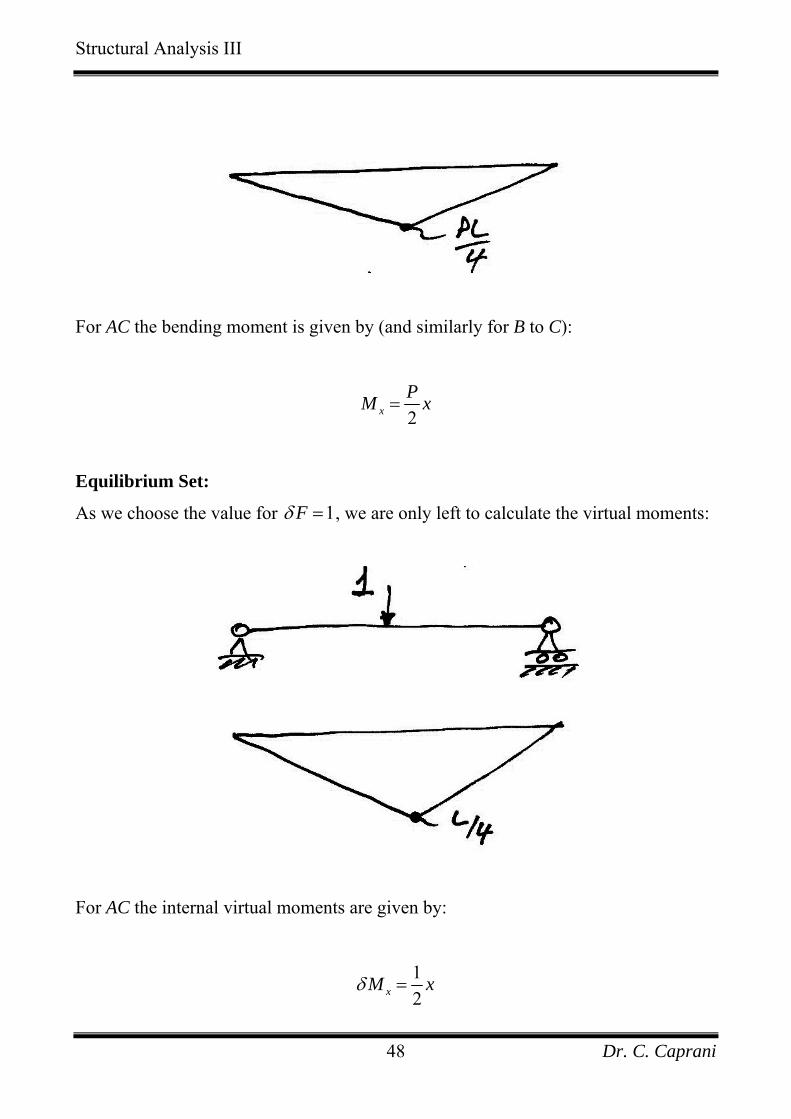
For AC the bending moment is given by (and similarly for B to C):
2xPM x=
Equilibrium Set:
As we choose the value for 1Fδ = , we are only left to calculate the virtual moments:
For AC the internal virtual moments are given by:
12xM xδ =
Dr. C. Caprani 48
Structural Analysis III
Virtual Work Equation
0
E I
i i i
WW W
y F Mi
δδ δ
δ θ δ
==
⋅ = ⋅∑ ∑
Substitute in the values we have for the real rotations and the virtual moments, and
use the fact that the bending moment diagrams are symmetrical:
2
0
2
0
22
0
23
0
3
3
1 2
2 12 2
24
2 3
6 8
48
Lx
x
L
L
L
My MEI
Py xEI
P x dxEI
P xEI
P LEIPL
dx
x dx
EI
δ⎡ ⎤⋅ = ⋅⎢ ⎥⎣ ⎦
⎛ ⎞ ⎛ ⎞= ⋅⎜ ⎟ ⎜ ⎟⎝ ⎠ ⎝ ⎠
=
⎡ ⎤= ⎢ ⎥
⎣ ⎦
= ⋅
=
∫
∫
∫
Which is a result we expected.
Dr. C. Caprani 49
Structural Analysis III
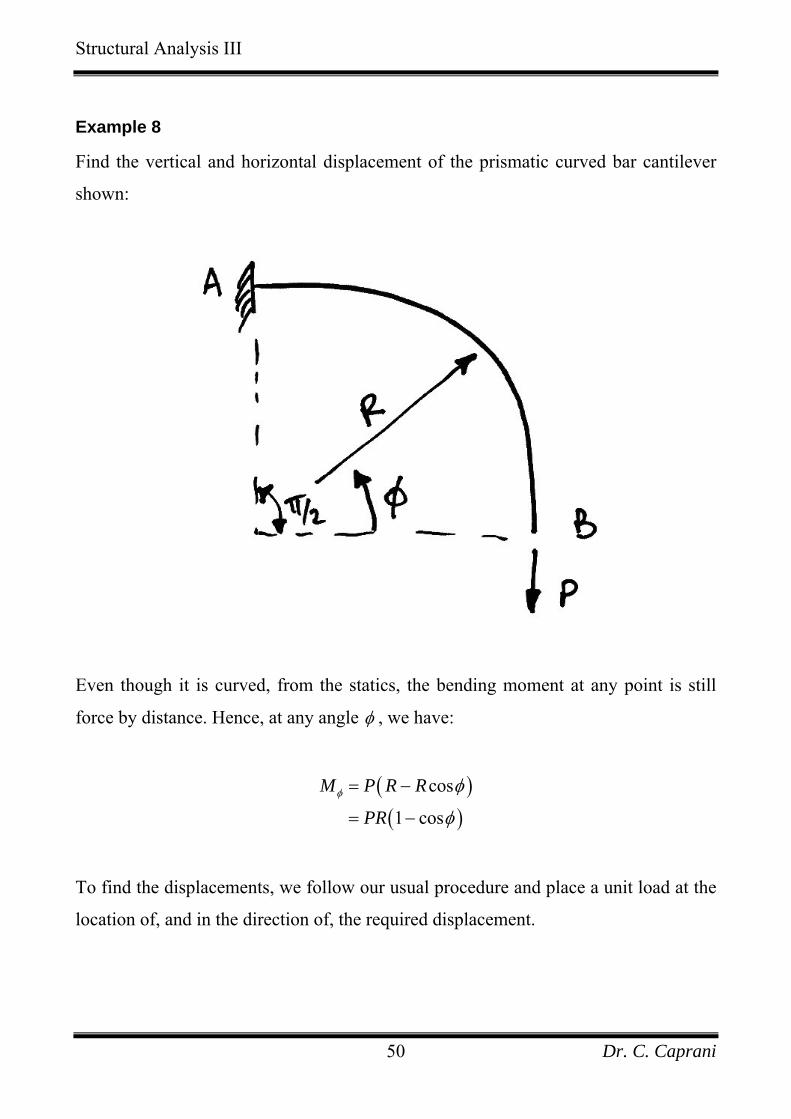
Example 8
Find the vertical and horizontal displacement of the prismatic curved bar cantilever
shown:
Even though it is curved, from the statics, the bending moment at any point is still
force by distance. Hence, at any angle φ , we have:
( )( )
cos
1 cos
M P R R
PRφ φ
φ
= −
= −
To find the displacements, we follow our usual procedure and place a unit load at the
location of, and in the direction of, the required displacement.
Dr. C. Caprani 50
Structural Analysis III
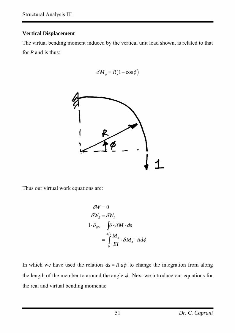
Vertical Displacement
The virtual bending moment induced by the vertical unit load shown, is related to that
for P and is thus:
( )1 cosM Rφδ φ= −
Thus our virtual work equations are:
2
0
0
1E I
BV
WW W
M ds
MM Rd
EI
πφ
φ
δδ δ
δ θ δ
δ φ
==
⋅ = ⋅ ⋅
= ⋅ ⋅
∫
∫
In which we have used the relation ds R dφ= to change the integration from along
the length of the member to around the angle φ . Next we introduce our equations for
the real and virtual bending moments:
Dr. C. Caprani 51
Structural Analysis III
( ) ( )
( )
( )
2
0
232
0
3 3
1 cos1 1
1 cos
3 4 5.42
BV
PRcosR Rd
EI
PR dEI
PR PREI EI
π
π
φδ φ φ
φ φ
π
−⋅ = ⋅ − ⋅
= − ⋅
= − ≈
∫
∫
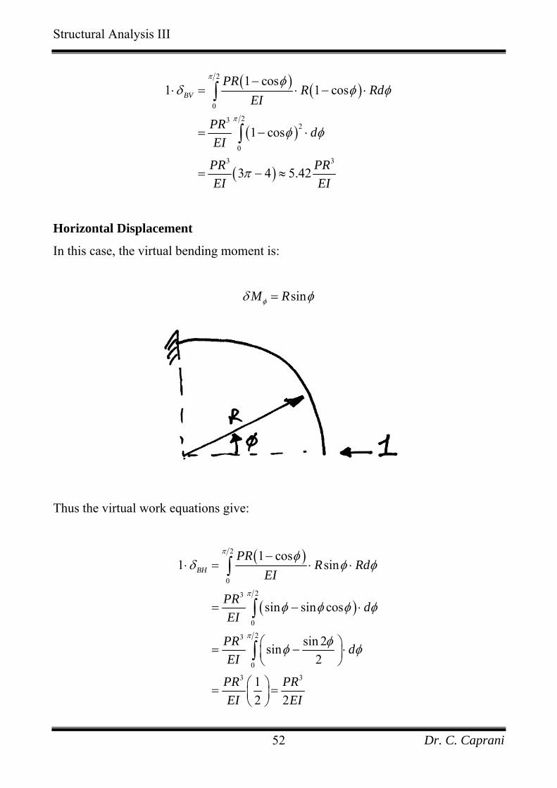
Horizontal Displacement
In this case, the virtual bending moment is:
sinM Rφδ φ=
Thus the virtual work equations give:
( )
( )
2
023
0
23
0
3 3
1 cos1 s
sin sin cos
sin 2sin2
12 2
BH
PRinR Rd
EI
PR dEI
PR dEI
PR PREI EI
π
π
π
φδ φ φ
φ φ φ
φ
φ
φ φ
−⋅ = ⋅ ⋅
= −
⎛ ⎞= − ⋅⎜ ⎟⎝ ⎠
⎛ ⎞= =⎜ ⎟⎝ ⎠
∫
∫
∫
⋅
Dr. C. Caprani 52
Structural Analysis III
4.4 Integration of Bending Moments
We are often faced with the integration of being moment diagrams when using virtual
work to calculate the deflections of bending members. And as bending moment
diagrams only have a limited number of shapes, a table of ‘volume’ integrals is used:
This table is at the back page of these notes for ease of reference.
Example 9
Using the table of volume integrals, verify the answer to Example 7.
In this case, the virtual work equation becomes:
[ ] [ ]
2
0
3
1 2
2 shape shape
2 13 4 4 2
48
Lx
x
x x
My M dxEI
y M MEI
PL L LEIPL
EI
δ
δ
⎡ ⎤⋅ = ⋅⎢ ⎥⎣ ⎦
= ×
⎡ ⎤= ⋅ ⋅ ⋅⎢ ⎥⎣ ⎦
=
∫
In which the formula 13
jkl is used from the table.
Dr. C. Caprani 53
Structural Analysis III
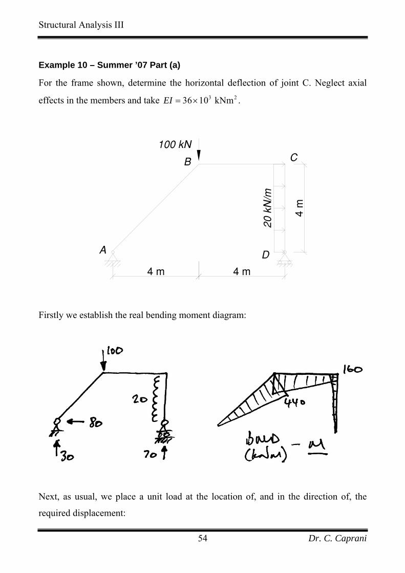
Example 10 – Summer ’07 Part (a)
For the frame shown, determine the horizontal deflection of joint C. Neglect axial
effects in the members and take 3 236 10 kNmEI = × .
4 m
4 m
A
B C
20 k
N/m
100 kN
4 m
D
Firstly we establish the real bending moment diagram:
Next, as usual, we place a unit load at the location of, and in the direction of, the
required displacement:
Dr. C. Caprani 54

Structural Analysis III
Now we have the following for the virtual work equation:
0
1E I
CH
WW W
M ds
M M dsEI
δδ δ
δ θ δ
δ
==
⋅ = ⋅ ⋅
= ⋅ ⋅
∫
∫
Next, using the table of volume integrals, we have:
( )( )( ) ( )( )( )1 1 1440 2 4 2 2 160 2 440 43 6
1659.3 1386.7
3046
AB BC
M M dsEI EI
EI EI
EI
δ⎧ ⎫⎡ ⎤ ⎡⋅ ⋅ = + + ⋅⎨ ⎬⎢ ⎥ ⎢⎣ ⎦ ⎣⎩ ⎭
= +
=
∫ ⎤⎥⎦
Hence:
33
3046 30461 1036 10CH EI
δ⋅ = = × =×
84.6 mm
Dr. C. Caprani 55
Structural Analysis III
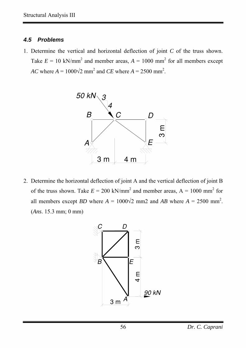
4.5 Problems
1. Determine the vertical and horizontal deflection of joint C of the truss shown.
Take E = 10 kN/mm2 and member areas, A = 1000 mm2 for all members except
AC where A = 1000√2 mm2 and CE where A = 2500 mm2.
A
B C D
E
3 m 4 m3
m
50 kN 34
2. Determine the horizontal deflection of joint A and the vertical deflection of joint B
of the truss shown. Take E = 200 kN/mm2 and member areas, A = 1000 mm2 for
all members except BD where A = 1000√2 mm2 and AB where A = 2500 mm2.
(Ans. 15.3 mm; 0 mm)
A
B E
C D
90 kN3 m
3 m
4 m
Dr. C. Caprani 56
Structural Analysis III
3. Verify that the deflection at the centre of a simply-supported beam under a
uniformly distributed load is given by:
45
384CwL
EIδ =
4. Show that the flexural deflection at the tip of a cantilever, when it is subjected to a
point load on the end is:
3
3BPLEI
δ =
5. Show that the rotation that occurs at the supports of a simply supported beam with
a point load in the middle is:
2
16CPL
EIθ =
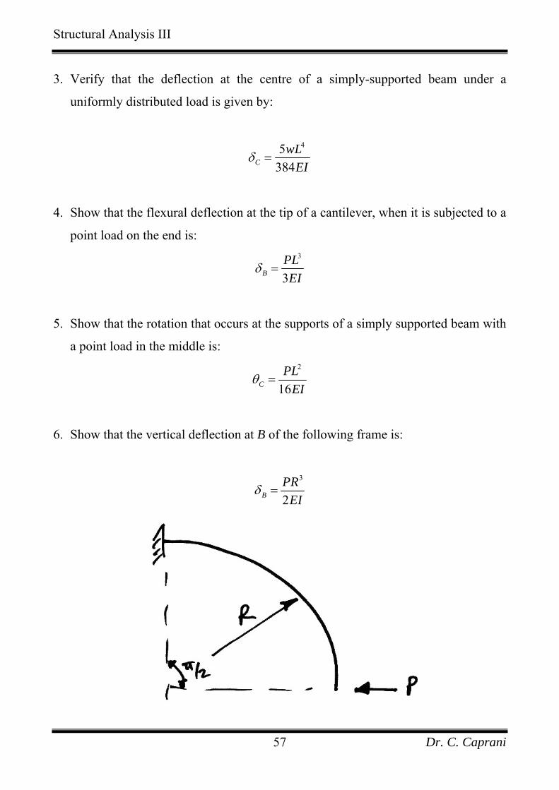
6. Show that the vertical deflection at B of the following frame is:
3
2BPR
EIδ =
Dr. C. Caprani 57

Structural Analysis III
7. For the frame of Example 10, using virtual work, verify the following
displacements in which the following directions are positive: vertical upwards;
horizontal to the right, and; clockwise:
• Rotation at A is 1176.3EI
− ;
• Vertical deflection at B is 3046EI
− ;
• Horizontal deflection at D is 8758.7EI
;
• Rotation at C is 1481.5EI
.
8. For the cantilever beam shown, show that the vertical deflection of B, allowing for
both flexural and shear deformation, is 3PL kPL
EI GA+ .
Dr. C. Caprani 58
Structural Analysis III
Problems 9 to 13 are considered Genius Level!
9. Show that the vertical deflection at the centre of a simply supported beam,
allowing for both flexural and shear deformation is 4 25
384 8wL kwL
EI G+
A.
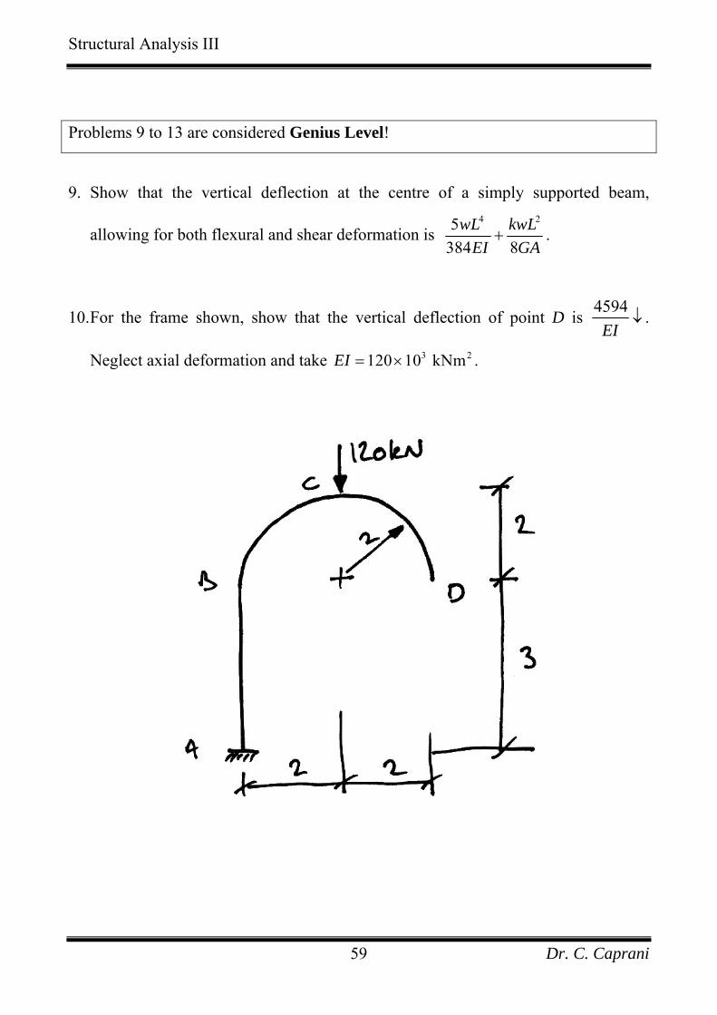
10. For the frame shown, show that the vertical deflection of point D is 4594EI
↓ .
Neglect axial deformation and take 3 2120 10 kNmEI = × .
Dr. C. Caprani 59
Structural Analysis III
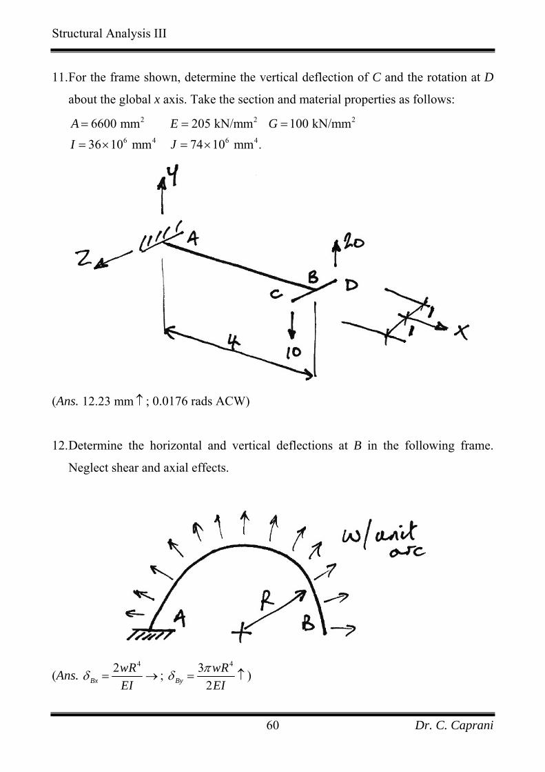
11. For the frame shown, determine the vertical deflection of C and the rotation at D
about the global x axis. Take the section and material properties as follows: 2 2
6 4 6 4
6600 mm 205 kN/mm 100 kN/mm36 10 mm 74 10 mm .
A E G 2
I J= = =
= × = ×
(Ans. 12.23 m ; 0.0176 rads ACW) m ↑
12. Determine the horizontal and vertical deflections at B in the following frame.
Neglect shear and axial effects.
(Ans. 42
BxwREI
δ = → ; 43
2BywREI
πδ = ↑ )
Dr. C. Caprani 60

Structural Analysis III
13. For the frame shown, neglecting shear effects, determine the vertical deflection of
points B and A.
(Ans. ( ) 3
3By
P wa bEI
δ+
= ↓ ; ( ) 33 4 213 8 3 2Ay
P wa bPa wa Pa wa abEI G
δ⎡ ⎤+ ⎛ ⎞+
= + + +⎢ ⎥ ⎜ ⎟⎝ ⎠⎣ ⎦ J
↓ )
Dr. C. Caprani 61
Structural Analysis III
5. Virtual Work for Indeterminate Structures
5.1 General Approach
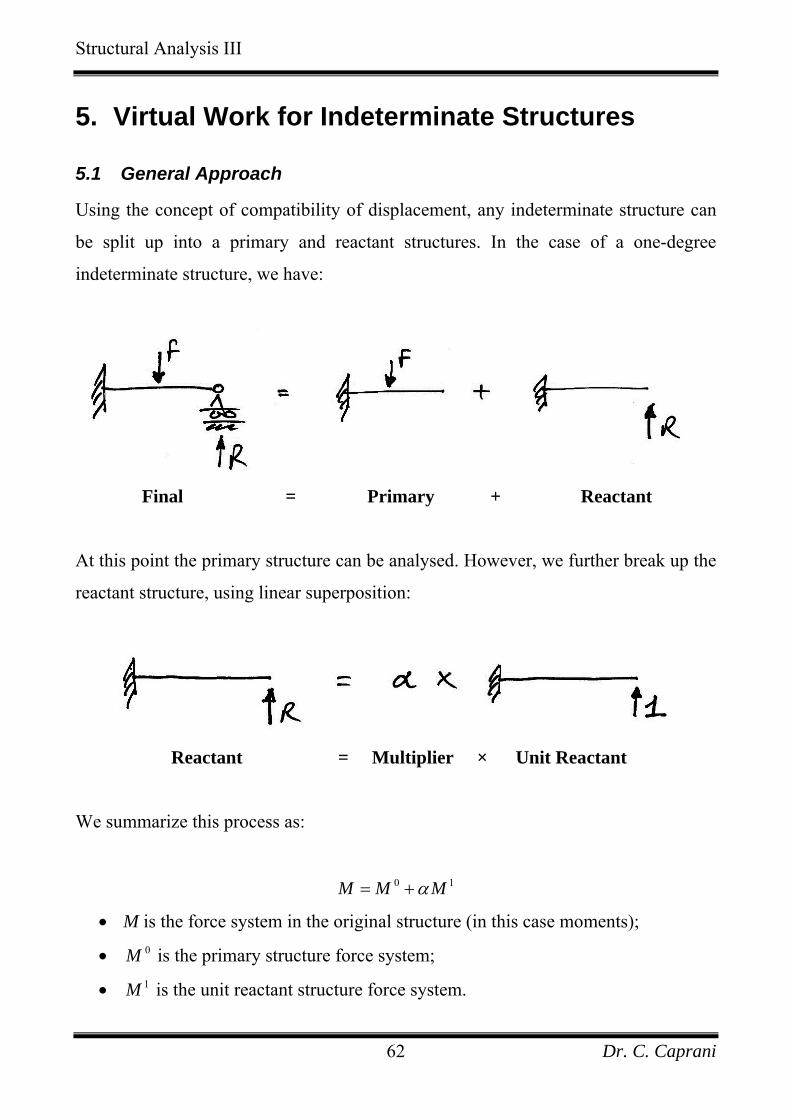
Using the concept of compatibility of displacement, any indeterminate structure can
be split up into a primary and reactant structures. In the case of a one-degree
indeterminate structure, we have:
Final = Primary + Reactant
At this point the primary structure can be analysed. However, we further break up the
reactant structure, using linear superposition:
Reactant = Multiplier × Unit Reactant
We summarize this process as:
0 1M M Mα= +
• M is the force system in the original structure (in this case moments);
• 0M is the primary structure force system;
• 1M is the unit reactant structure force system.
Dr. C. Caprani 62
Structural Analysis III
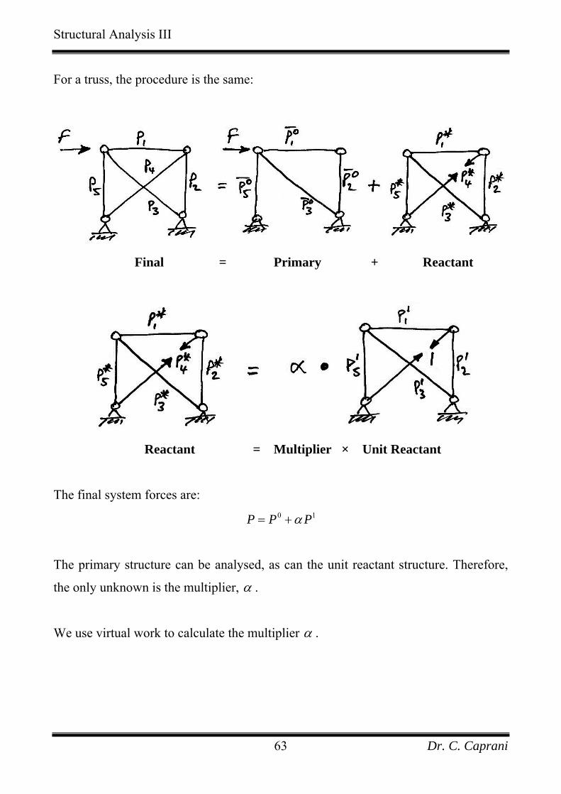
For a truss, the procedure is the same:
Final = Primary + Reactant
Reactant = Multiplier × Unit Reactant
The final system forces are:
0 1P P Pα= +
The primary structure can be analysed, as can the unit reactant structure. Therefore,
the only unknown is the multiplier, α .
We use virtual work to calculate the multiplier α .
Dr. C. Caprani 63
Structural Analysis III
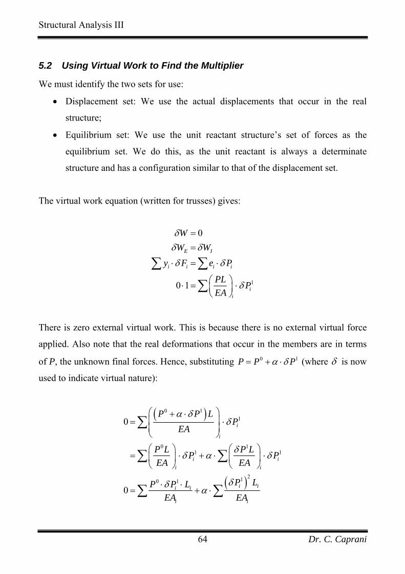
5.2 Using Virtual Work to Find the Multiplier
We must identify the two sets for use:
• Displacement set: We use the actual displacements that occur in the real
structure;
• Equilibrium set: We use the unit reactant structure’s set of forces as the
equilibrium set. We do this, as the unit reactant is always a determinate
structure and has a configuration similar to that of the displacement set.
The virtual work equation (written for trusses) gives:
1
0
0 1
E I
i i i i
ii
WW W
y F e P
PL PEA
δδ δ
δ δ
δ
==
⋅ = ⋅
⎛ ⎞⋅ = ⋅⎜ ⎟⎝ ⎠
∑ ∑
∑
There is zero external virtual work. This is because there is no external virtual force
applied. Also note that the real deformations that occur in the members are in terms
of P, the unknown final forces. Hence, substituting 0 1P P Pα δ= + ⋅ (where δ is now
used to indicate virtual nature):
( )
( )
0 11
0 11 1
210 1
0
0
i
i
i ii i
i ii i
i i
P P LP
EA
P L P LP PEA EA
P LP P LEA EA
α δδ
δδ α δ
δδ α
⎛ ⎞+ ⋅⎜ ⎟= ⋅⎜ ⎟⎝ ⎠
⎛ ⎞ ⎛ ⎞= ⋅ + ⋅⎜ ⎟ ⎜ ⎟
⎝ ⎠ ⎝ ⎠
⋅ ⋅= + ⋅
∑
∑ ∑
∑ ∑
⋅
Dr. C. Caprani 64

Structural Analysis III
For beams and frames, the same equation is:
( )210 1
0 0
0L L
ii
i i
MM M dx dxEI EI
δδ α⋅= + ⋅∑ ∑∫ ∫
Thus in both bases we have a single equation with only one unknown, α . We can
establish values for the other two terms and then solve for α and the structure as a
whole.
Dr. C. Caprani 65
Structural Analysis III
5.3 Indeterminate Trusses
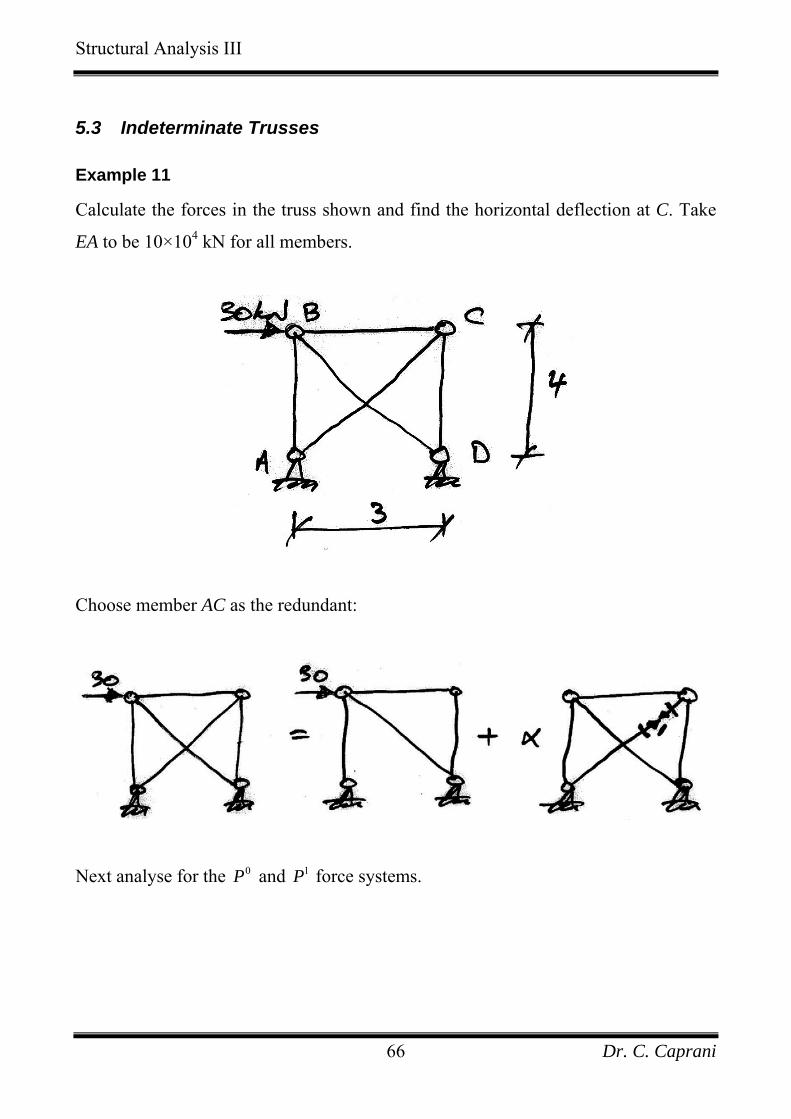
Example 11
Calculate the forces in the truss shown and find the horizontal deflection at C. Take
EA to be 10×104 kN for all members.
Choose member AC as the redundant:
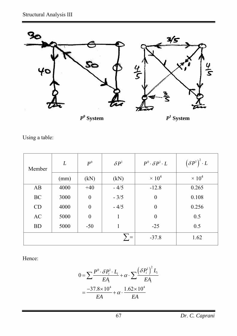
Next analyse for the 0P and 1P force systems.
Dr. C. Caprani 66
Structural Analysis III
P0 System P1 System
Using a table:
L 0P 1Pδ 0 1P P Lδ⋅ ⋅ ( )21P Lδ ⋅ Member
(mm) (kN) (kN) × 104 × 104
AB
BC
CD
AC
BD
4000
3000
4000
5000
5000
+40
0
0
0
-50
- 4/5
- 3/5
- 4/5
1
1
-12.8
0
0
0
-25
0.265
0.108
0.256
0.5
0.5
=∑ -37.8 1.62
Hence:
( )210 1
4 4
0
37.8 10 1.62 10
i ii i
i i
P LP P LEA EA
EA EA
δδ α
α
⋅ ⋅= + ⋅
− × ×= + ⋅
∑ ∑
Dr. C. Caprani 67
Structural Analysis III
And so
37.8 23.331.62
α −= − =
The remaining forces are obtained from the compatibility equation:
0P 1Pδ 0 1P P Pα δ= + ⋅Member
(kN) (kN) (kN) AB
BC
CD
AC
BD
+40
0
0
0
-50
- 4/5
- 3/5
- 4/5
1
1
21.36
-14
-18.67
23.33
-26.67
Note that the redundant always has a force the same as the multiplier.
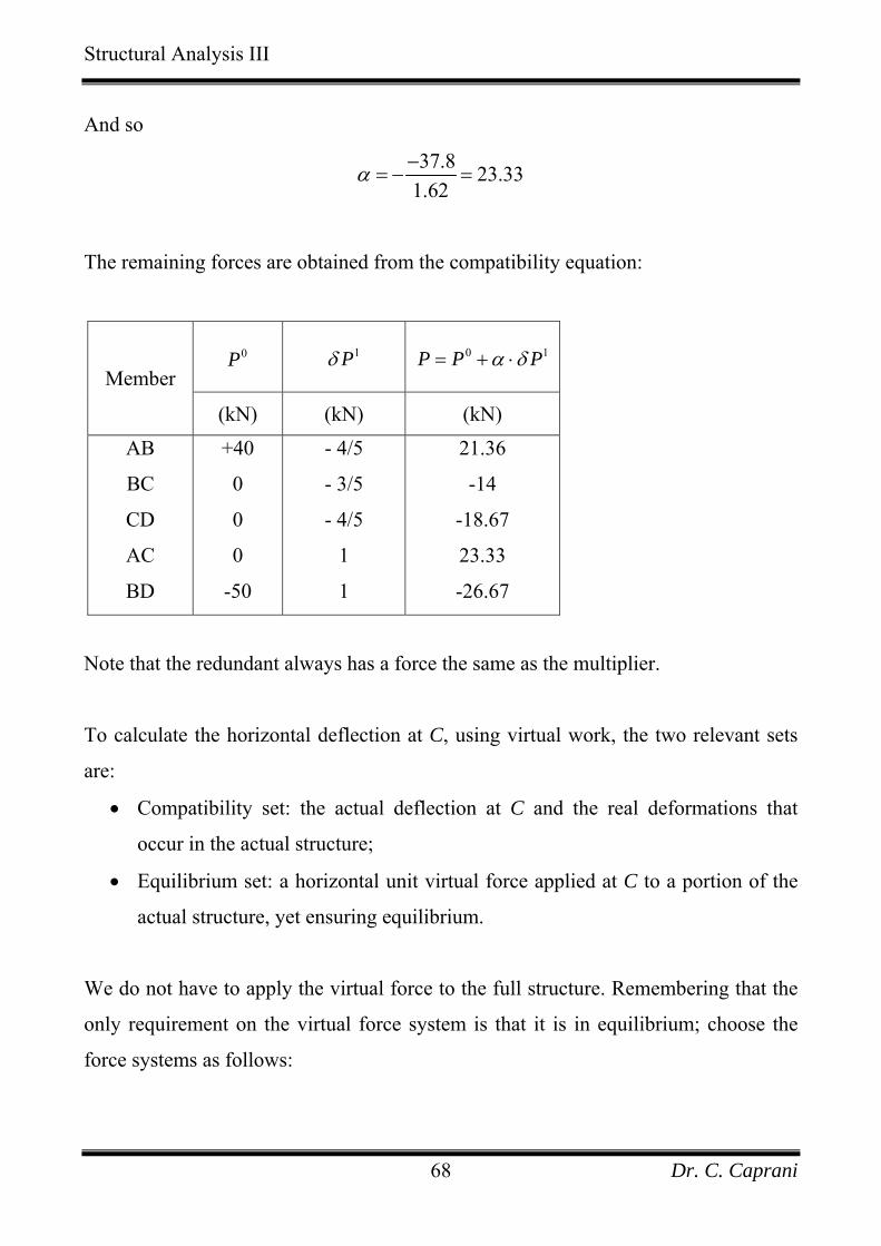
To calculate the horizontal deflection at C, using virtual work, the two relevant sets
are:
• Compatibility set: the actual deflection at C and the real deformations that
occur in the actual structure;
• Equilibrium set: a horizontal unit virtual force applied at C to a portion of the
actual structure, yet ensuring equilibrium.
We do not have to apply the virtual force to the full structure. Remembering that the
only requirement on the virtual force system is that it is in equilibrium; choose the
force systems as follows:
Dr. C. Caprani 68
Structural Analysis III
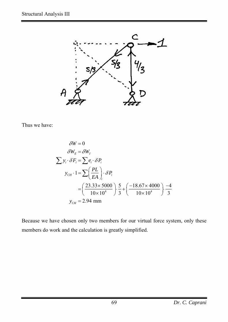
Thus we have:
4 4
0
1
23.33 5000 5 18.67 4000 410 10 3 10 10 3
2.94 mm
E I
i i i i
CH ii
CH
WW W
y F e P
PLy PEA
y
δδ δ
δ δ
δ
==
⋅ = ⋅
⎛ ⎞⋅ = ⋅⎜ ⎟⎝ ⎠
× − ×⎛ ⎞ ⎛= ⋅ +⎜ ⎟ ⎜× ×⎝ ⎠ ⎝=
∑ ∑
∑−⎞ ⋅⎟
⎠
Because we have chosen only two members for our virtual force system, only these
members do work and the calculation is greatly simplified.
Dr. C. Caprani 69
Structural Analysis III
5.4 Indeterminate Frames
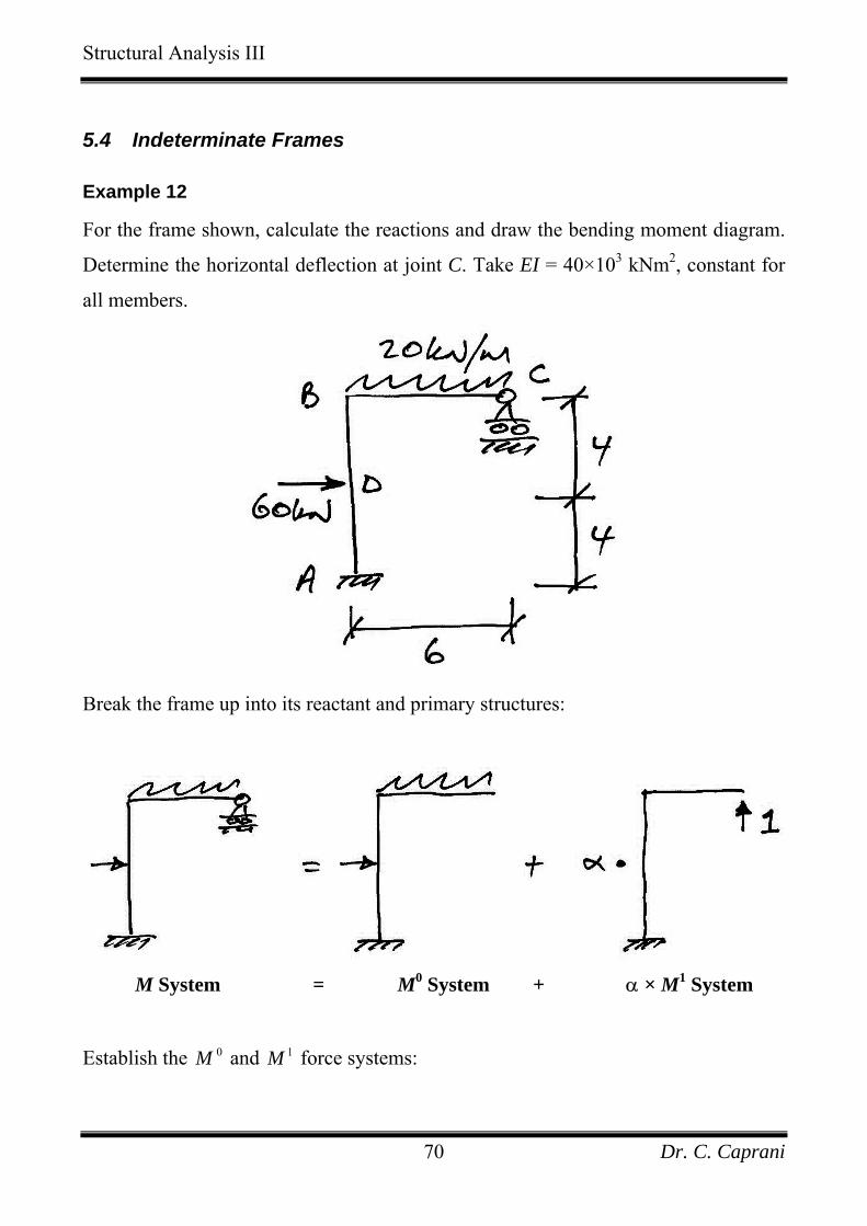
Example 12
For the frame shown, calculate the reactions and draw the bending moment diagram.
Determine the horizontal deflection at joint C. Take EI = 40×103 kNm2, constant for
all members.
Break the frame up into its reactant and primary structures:
M System = M0 System + α × M1 System
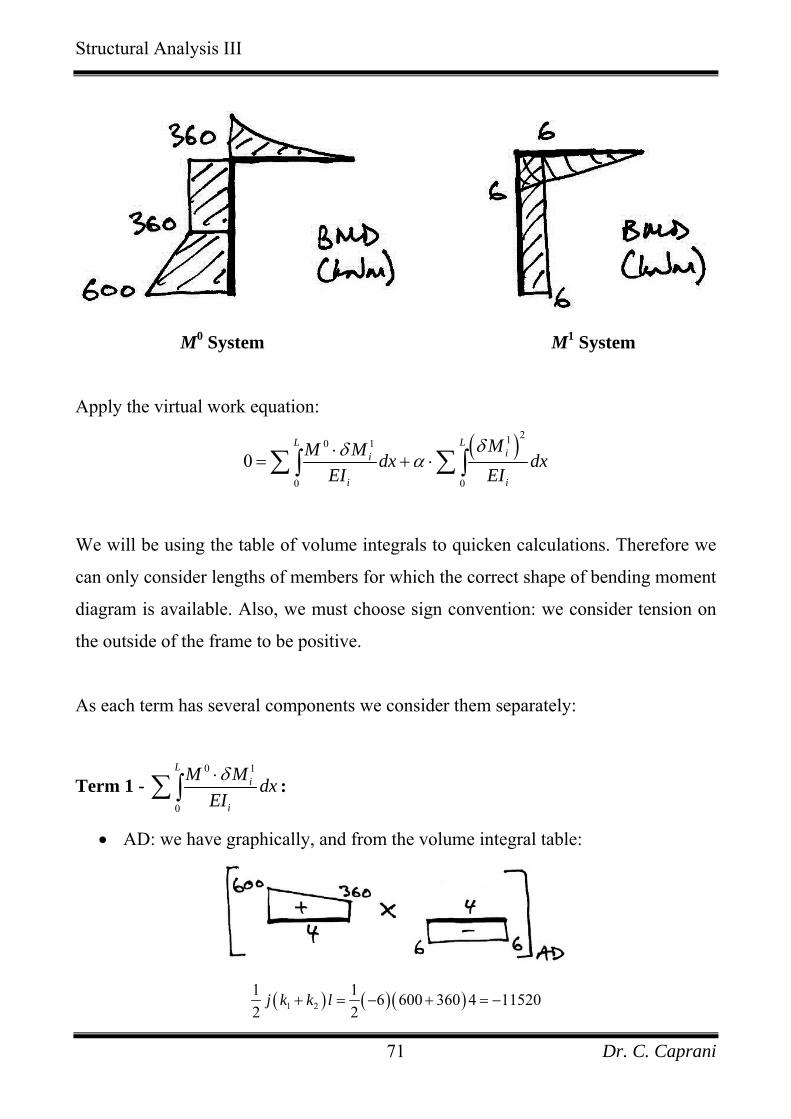
Establish the 0M and 1M force systems:
Dr. C. Caprani 70
Structural Analysis III
M0 System M1 System
Apply the virtual work equation:
( )210 1
0 0
0L L
ii
i i
MM M dx dxEI EI
δδ α⋅= + ⋅∑ ∑∫ ∫
We will be using the table of volume integrals to quicken calculations. Therefore we
can only consider lengths of members for which the correct shape of bending moment
diagram is available. Also, we must choose sign convention: we consider tension on
the outside of the frame to be positive.
As each term has several components we consider them separately:
Term 1 - 0 1
0
Li
i
M M dxEIδ⋅∑∫ :
• AD: we have graphically, and from the volume integral table:
( ) ( )( )1 21 1 6 600 360 4 115202 2
j k k l+ = − + = −
Dr. C. Caprani 71
Structural Analysis III
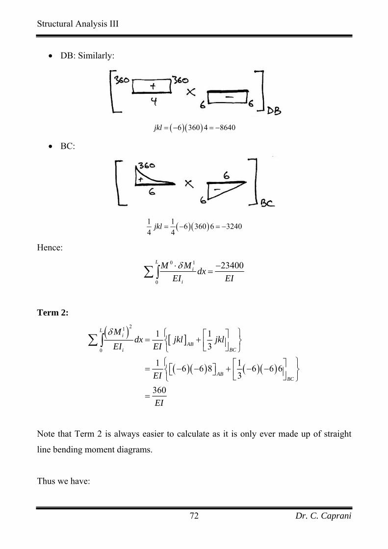
• DB: Similarly:
( )( )6 360 4 8640jkl = − = −
• BC:
( )( )1 1 6 360 6 32404 4
jkl = − = −
Hence: 0 1
0
23400Li
i
M M dxEI Eδ⋅ −
=∑∫ I
Term 2:
( ) [ ]
( )( ) ( )( )
21
0
1 13
1 16 6 8 6 6 63
360
Li
ABBCi
ABBC
Mdx jkl jkl
EI EI
EI
EI
δ ⎧ ⎫⎡ ⎤= +⎨ ⎬⎢ ⎥⎣ ⎦⎩ ⎭⎧ ⎫⎡ ⎤= − − + − −⎡ ⎤⎨ ⎬⎣ ⎦ ⎢ ⎥⎣ ⎦⎩ ⎭
=
∑∫
Note that Term 2 is always easier to calculate as it is only ever made up of straight
line bending moment diagrams.
Thus we have:
Dr. C. Caprani 72
Structural Analysis III
( )210 1
0 0
0
23400 360
L Lii
i i
MM M dx dxEI EI
EI EI
δδ α
α
⋅= + ⋅
−= + ⋅
∑ ∑∫ ∫
And so
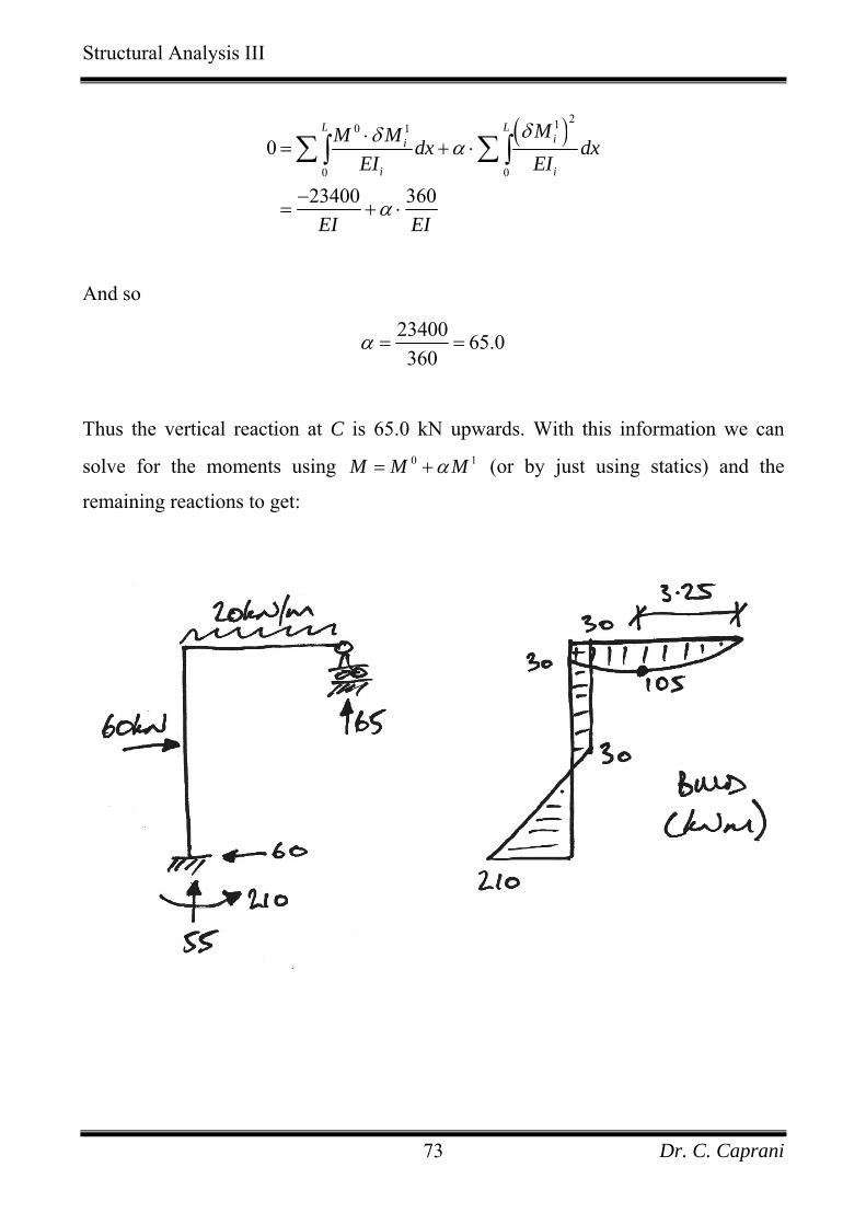
23400 65.0360
α = =
Thus the vertical reaction at C is 65.0 kN upwards. With this information we can
solve for the moments using 0 1M M Mα= + (or by just using statics) and the
remaining reactions to get:
Dr. C. Caprani 73
Structural Analysis III
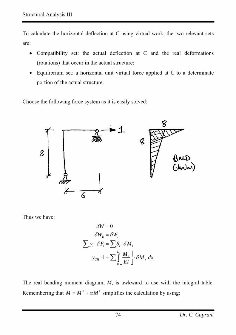
To calculate the horizontal deflection at C using virtual work, the two relevant sets
are:
• Compatibility set: the actual deflection at C and the real deformations
(rotations) that occur in the actual structure;
• Equilibrium set: a horizontal unit virtual force applied at C to a determinate
portion of the actual structure.
Choose the following force system as it is easily solved:
Thus we have:
0
0
1
E I
i i i i
Lx
CH x
WW W
y F M
My MEI
dx
δδ δ
δ θ δ
δ
==
⋅ = ⋅
⎡ ⎤⋅ = ⋅⎢ ⎥⎣ ⎦
∑ ∑
∑∫
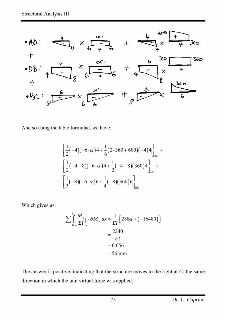
The real bending moment diagram, M, is awkward to use with the integral table.
Remembering that 0 1M M Mα= + simplifies the calculation by using:
Dr. C. Caprani 74
Structural Analysis III
And so using the table formulae, we have:
( )( ) ( )( )
( )( ) ( )( )
( )( ) ( )( )
1 14 6 4 2 360 600 4 42 61 14 8 6 4 4 8 360 42 21 18 6 6 8 360 63 4
AD
DB
BC
α
α
α
⎡ ⎤− − ⋅ + ⋅ + −⎢ ⎥⎣ ⎦
⎡ ⎤− − − ⋅ + − − +⎢ ⎥⎣ ⎦
⎡ ⎤− − ⋅ + −⎢ ⎥⎣ ⎦
+
Which gives us:
( )0
1 288 16480
2240
0.05656 mm
Lx
xM M dxEI EI
EI
δ α⎡ ⎤ ⋅ = + −⎡ ⎤⎣ ⎦⎢ ⎥⎣ ⎦
=
==
∑∫
The answer is positive, indicating that the structure moves to the right at C: the same
direction in which the unit virtual force was applied.
Dr. C. Caprani 75
Structural Analysis III
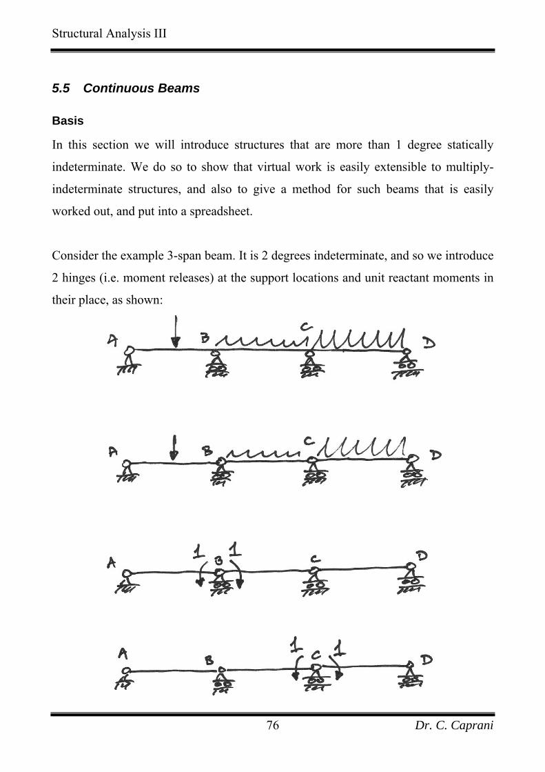
5.5 Continuous Beams
Basis
In this section we will introduce structures that are more than 1 degree statically
indeterminate. We do so to show that virtual work is easily extensible to multiply-
indeterminate structures, and also to give a method for such beams that is easily
worked out, and put into a spreadsheet.
Consider the example 3-span beam. It is 2 degrees indeterminate, and so we introduce
2 hinges (i.e. moment releases) at the support locations and unit reactant moments in
their place, as shown:
Dr. C. Caprani 76

Structural Analysis III
Alongside these systems, we have their bending moment diagrams:
Using the idea of the multiplier and superposition again, we can see that:
0 11 2
2M M Mα δ α δ= + ⋅ + ⋅ M
The virtual work equation is:
0
0 1E I
WW W
M
δδ δ
θ δ
==
⋅ = ⋅∑∫
Dr. C. Caprani 77

Structural Analysis III
There is no external virtual work done since the unit moments are applied internally.
Since we have two virtual force systems in equilibrium and one real compatible
system, we have two equations:
10 M MEI
δ= ⋅∑∫ and 20 M MEI
δ= ⋅∑∫
For the first equation, expanding the expression for the real moment system, M:
( )0 1 21 2 1
0 1 1 1 2 1
1 2
0
0
M M MM
EIM M M M M M
EI EI EI
α δ α δδ
δ δ δ δ δα α
+ ⋅ + ⋅⋅ =
⋅ ⋅ ⋅+ +
∑∫
∫ ∫ ∫ =
In which we’ve dropped the summation over all members – it being understood that
we sum for all members. Similarly for the second virtual moments, we have:
0 2 1 2 2 2
1 2 0M M M M M MEI EI EIδ δ δ δ δα α⋅ ⋅ ⋅
+ +∫ ∫ ∫ =
Thus we have two equations and so we can solve for 1α and 2α . Usually we write
this as a matrix equation:
0 1 1 1 2 1
10 2 1 2 2 2
2
00
M M M M M MEI EI EI
M M M M M MEI EI EI
δ δ δ δ δααδ δ δ δ δ
⎧ ⎫ ⎡ ⎤⋅ ⋅ ⋅⎪ ⎪ ⎢ ⎥ ⎧ ⎫ ⎧ ⎫⎪ ⎪ ⎢ ⎥+ =⎨ ⎬ ⎨ ⎬
⋅ ⋅ ⋅⎢ ⎥ ⎩ ⎭⎩ ⎭⎪ ⎪⎢ ⎥⎪ ⎪⎩ ⎭ ⎣ ⎦
∫ ∫ ∫
∫ ∫ ∫⎨ ⎬
Each of the integral terms is easily found using the integral tables, and the equation
solved.
Dr. C. Caprani 78
Structural Analysis III
Dr. C. Caprani 79
Structural Analysis III
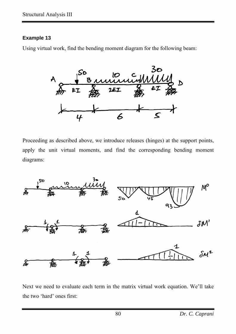
Example 13
Using virtual work, find the bending moment diagram for the following beam:
Proceeding as described above, we introduce releases (hinges) at the support points,
apply the unit virtual moments, and find the corresponding bending moment
diagrams:
Next we need to evaluate each term in the matrix virtual work equation. We’ll take
the two ‘hard’ ones first:
Dr. C. Caprani 80
Structural Analysis III
• ( )( )( ) ( )( )( )
( )
0 1 1 1 1 150 1 4 2 45 1 66 2 3
1 9550 45
AB BC
M MEI EI EI
EI EI
δ⋅ ⎡ ⎤ ⎡= − + + −⎢ ⎥ ⎢⎣ ⎦ ⎣
= − − = −
∫ ⎤⎥⎦
Note that since 1 0Mδ = for span CD, there is no term for it above. Similarly, for the
following evaluation, there will be no term for span AB:
• ( )( )( ) ( )( )( )
( )
0 2 1 1 1 145 1 6 93.75 1 52 3 31 201.2545 156.25
BC CD
M MEI EI EI
EI EI
δ⋅ ⎡ ⎤ ⎡= − + −⎢ ⎥ ⎢⎣ ⎦ ⎣
= − − = −
∫ ⎤⎥⎦
The following integrals are more straightforward since they are all triangles:
• ( )( )( ) ( )( )( )1 1 1 1 1 1 2.3331 1 4 1 1 6
3 2 3AB BC
M MEI EI EI E
δ δ⋅ ⎡ ⎤ ⎡ ⎤= − − + − − =⎢ ⎥ ⎢ ⎥⎣ ⎦ ⎣ ⎦∫ I
• ( )( )( )2 1 1 1 0.51 1 6
2 6 BC
M MEI EI
δ δ⋅ ⎡ ⎤= − − =⎢ ⎥⎣ ⎦∫ EI
• 1 2 0.5M MEI E
δ δ⋅=∫ I
, since it is equal to 2 1M MEI
δ δ⋅∫ by the commutative
property of multiplication.
• ( )( )( ) ( )( )( )2 2 1 1 1 1 2.6671 1 6 1 1 5
2 3 3BC CD
M MEI EI EI E
δ δ⋅ ⎡ ⎤ ⎡ ⎤= − − + − − =⎢ ⎥ ⎢ ⎥⎣ ⎦ ⎣ ⎦∫ I
With all the terms evaluated, enter them into the matrix equation:
Dr. C. Caprani 81

Dr. C. Caprani 82
From these we get the final BMD:
Structural Analysis III
1
2
95 2.333 0.5 01 1201.25 0.5 2.667 0EI EI
αα
− ⎧ ⎫⎧ ⎫ ⎡ ⎤ ⎧ ⎫+ =⎨ ⎬ ⎨ ⎬ ⎨ ⎬⎢ ⎥−⎩ ⎭ ⎣ ⎦ ⎩ ⎭⎩ ⎭
( )
And solve, as follows:
1
2
1
2
2.333 0.5 950.5 2.667 201.25
2.667 0.5 9510.5 2.333 201.252.333 2.667 0.5 0.5
25.5770.67
αα
αα
⎧ ⎫⎡ ⎤ ⎧ ⎫=⎨ ⎬ ⎨ ⎬⎢ ⎥
⎣ ⎦ ⎩ ⎭⎩ ⎭−⎧ ⎫ ⎡ ⎤ ⎧ ⎫
=⎨ ⎬ ⎨ ⎬⎢ ⎥−⋅ − ⋅ ⎣ ⎦ ⎩ ⎭⎩ ⎭⎧ ⎫
= ⎨ ⎬
0 1 21 2Now using our superposition equation for moments,
M M M Mα δ α δ= + ⋅ + ⋅
0 25.57 1 70.67 0 25.570 25.57 0 70.67 1 70.67 kNm
B
C
MM
= + ⋅ + ⋅ == + ⋅ + ⋅ =
,
we can show that the multipliers are just the hogging support moments:
⎩ ⎭
kNm

Structural Analysis III
Dr. C. Caprani 83
Spreadsheet Solution
A simple spreadsheet for a 3-span beam with centre-span point load and UDL capabilities, showing Example 13, is:
Span 1 Span 2 Span 3 VW Equations
Length m 4 6 51 2 150 0 00 10 30
EI x -95.000 + 2.333 0.500 * alpha1 = 0PL kN -201.250 0.500 2.667 alpha2 0UDL kN/m
BMDs PL 50 0 0 2.333 0.500 * alpha1 = 95.000UDL 0 45 93.75 0.500 2.667 alpha2 201.250
alpha1 = 0.446512 -0.083721 * 95.000M0 x M1 Span 1 Span 2 Span 3 Totals alpha2 -0.083721 0.390698 201.250PL -50.000 0.000 0.000UDL 0.000 -90.000 0.000 alpha1 = 25.57Total -50.000 -45.000 0.000 -95.000 alpha2 70.67
M1 x M1 Span 1 Span 2 Span 3Total 1.333 1.000 0.000 2.333
Mid-Span and Support MomentsM2 x M1 Span 1 Span 2 Span 3 Mab 37.2 kNmTotal 0.000 0.500 0.000 0.500 Mb -25.6 kNm
Mbc -3.1 kNmM0 x M2 Span 1 Span 2 Span 3 Mc -70.7 kNmPL 0.000 0.000 0.000 Mcd 58.4 kNmUDL 0.000 -90.000 -156.250Total 0.000 -45.000 -156.250 -201.250
M1 x M2 Span 1 Span 2 Span 3Total 0.000 0.500 0.000 0.500
M2 x M2 Span 1 Span 2 Span 3Total 0.000 1.000 1.667 2.667
Structural Analysis III
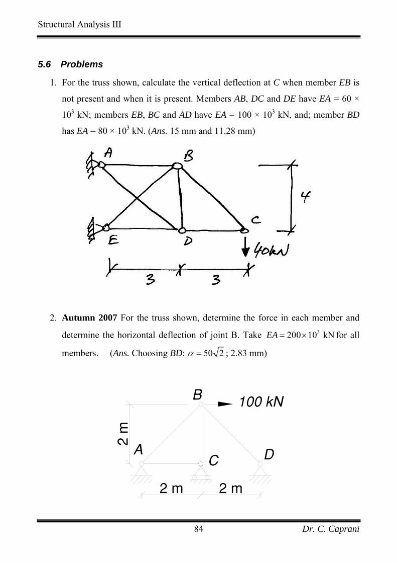
5.6 Problems
1. For the truss shown, calculate the vertical deflection at C when member EB is
not present and when it is present. Members AB, DC and DE have EA = 60 ×
103 kN; members EB, BC and AD have EA = 100 × 103 kN, and; member BD
has EA = 80 × 103 kN. (Ans. 15 mm and 11.28 mm)
2. Autumn 2007 For the truss shown, determine the force in each member and
determine the horizontal deflection of joint B. Take 3200 10 kNEA = × for all
members. (Ans. Choosing BD: 50 2α = ; 2.83 mm)
AC
B
D
100 kN
2 m 2 m
2 m
Dr. C. Caprani 84

Structural Analysis III
3. For the frame shown, calculate the bending moment diagram, and verify the
following deflections: 856.2Bx EI
δ = → and 327.6Cy EIδ = ↓ . (Ans.
) 30.1 kNmBM =
4. Summer 2007, Part (b): For the frame shown, draw the bending moment
diagram and determine the horizontal deflection of joint C. Neglect axial
effects in the members and take 336 10 kNm2EI = × . (Ans. ;
19.0 mm)
75.8 kNDH =
4 m
4 m
A
B C
20 k
N/m
100 kN
4 m
D
Dr. C. Caprani 85

Structural Analysis III
5. For the beam of Example 13, show that the deflections at the centre of each
span, taking downwards as positive, are:
• Span AB: 41.1EI
;
• Span BC: 23.9EI
− ;
• Span CD: 133.72EI
.
6. Using virtual work, analyse the following prismatic beam to show that the
support moments are 51.3 kNmBM = and 31.1 kNmCM = , and draw the
bending moment diagram:
Dr. C. Caprani 86
Structural Analysis III
6. Virtual Work for Self-Stressed Structures
6.1 Background
Introduction
Self-stressed structures are structures that have stresses induced, not only by external
loading, but also by any of the following:
• Temperature change of some of the members (e.g. solar gain);
• Lack of fit of members from fabrication:
o Error in the length of the member;
o Ends not square and so a rotational lack of fit;
• Incorrect support location from imperfect construction;
• Non-rigid (i.e. spring) supports due to imperfect construction.
Since any form of fabrication or construction is never perfect, it is very important for
us to know the effect (in terms of bending moment, shear forces etc.) that such errors,
even when small, can have on the structure.
Here we introduce these sources, and examine their effect on the virtual work
equation. Note that many of these sources of error can exist concurrently. In such
cases we add together the effects from each source.
Dr. C. Caprani 87
Structural Analysis III
Temperature Change
The source of self-stressing in this case is that the temperature change causes a
member to elongate:
( )TL L Tα∆ = ∆
where α is the coefficient of linear thermal expansion (change in length, per unit
length, per degree Celsius), L is the original member length and is the
temperature change.
T∆
Since temperature changes change the length of a member, the internal virtual work
is affected. Assuming a truss member is being analysed, we now have changes in
length due to force and temperature, so the total change in length of the member is:
( )PLe L TEA
α= + ∆
Hence the internal virtual work for this member is:
( )
IW e PPL L T PEA
δ δ
α δ
= ⋅
⎛ ⎞= + ∆ ⋅⎜ ⎟⎝ ⎠
Dr. C. Caprani 88

Structural Analysis III
Linear Lack of Fit
For a linear lack of fit, the member needs to be artificially elongated or shortened to
fit it into place, thus introducing additional stresses. This is denoted:
Lλ
Considering a truss member subject to external loading, the total change in length
will be the deformation due to loading and the linear lack of fit:
LPLeEA
λ= +
Hence the internal virtual work for this member is:
I
L
W e PPL PEA
δ δ
λ δ
= ⋅
⎛ ⎞= + ⋅⎜ ⎟⎝ ⎠
Dr. C. Caprani 89
Structural Analysis III
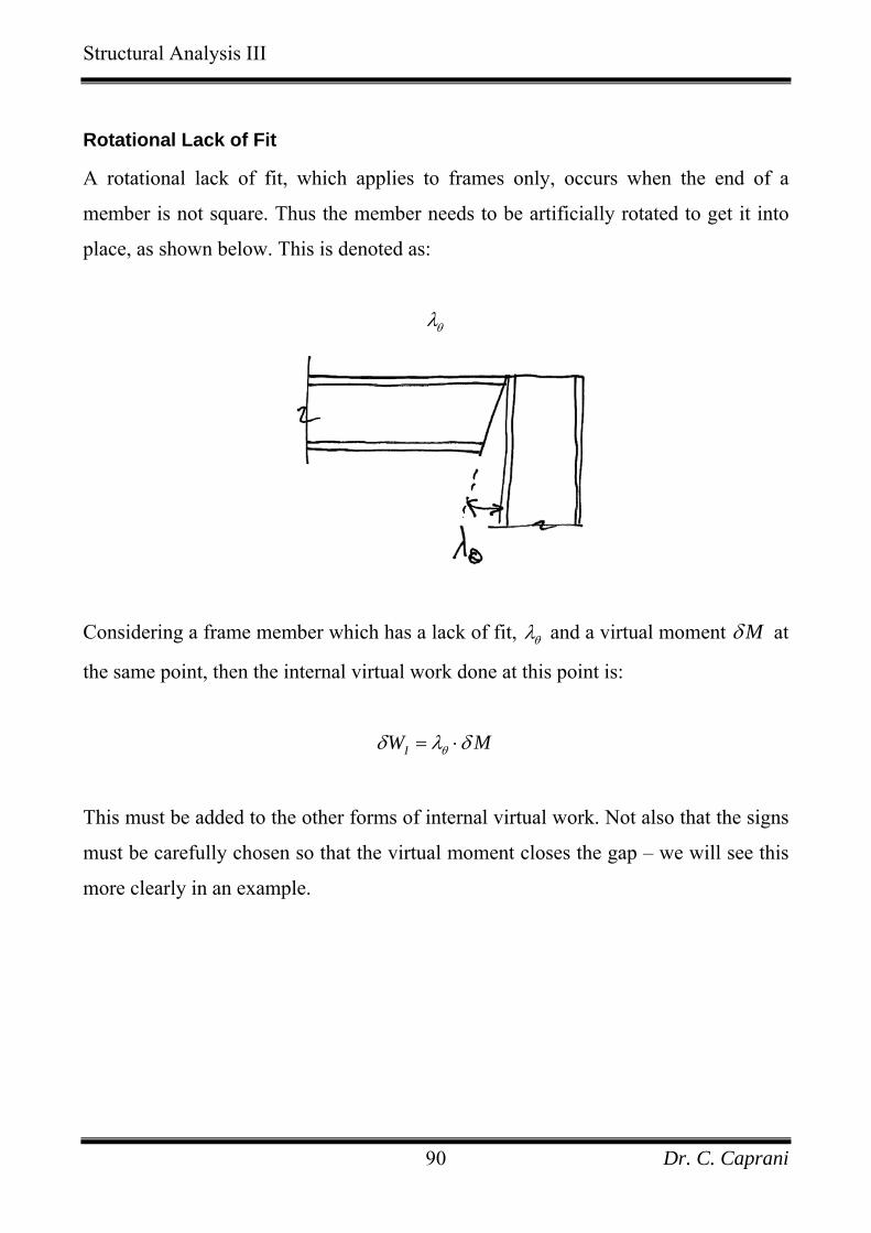
Rotational Lack of Fit
A rotational lack of fit, which applies to frames only, occurs when the end of a
member is not square. Thus the member needs to be artificially rotated to get it into
place, as shown below. This is denoted as:
θλ
Considering a frame member which has a lack of fit, θλ and a virtual moment Mδ at
the same point, then the internal virtual work done at this point is:
IW Mθδ λ δ= ⋅
This must be added to the other forms of internal virtual work. Not also that the signs
must be carefully chosen so that the virtual moment closes the gap – we will see this
more clearly in an example.
Dr. C. Caprani 90

Structural Analysis III
Errors in Support Location
The support can be misplaced horizontally and/or vertically. It is denoted:
Sλ
A misplaced support affects the external movements of a structure, and so contributes
to the external virtual work. Denoting the virtual reaction at the support, in the
direction of the misplacement as Rδ , then we have:
e SW Rδ λ δ= ⋅
Dr. C. Caprani 91
Structural Analysis III
Spring Supports
For spring supports we will know the spring constant for the support, denoted:
Sk
Since movements of a support are external, spring support movements affect the
external virtual work. The real displacement S∆ that occurs is:
S SR k∆ =
In which R is the real support reaction in the direction of the spring. Further, since R
will be known in terms of the multiplier and virtual reaction, Rδ , we have:
0R R Rα δ= + ⋅
Hence:
( )0S SR R kα δ∆ = + ⋅
And so the external work done is:
( )20
e S
S S
W R
RR Rk k
δ δ
δδ α
= ∆ ⋅
= ⋅ + ⋅
The only unknown here is α which is solved for from the virtual work equation.
Dr. C. Caprani 92
Structural Analysis III
6.2 Trusses
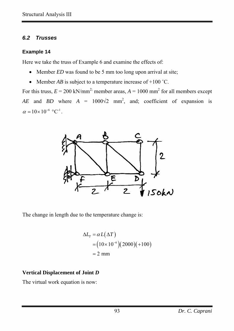
Example 14
Here we take the truss of Example 6 and examine the effects of:
• Member ED was found to be 5 mm too long upon arrival at site;
• Member AB is subject to a temperature increase of +100 ˚C.
For this truss, E = 200 kN/mm2; member areas, A = 1000 mm2 for all members except
AE and BD where A = 1000√2 mm2, and; coefficient of expansion is 6 -10 10 C 1α −= × ° .
The change in length due to the temperature change is:
( )( )( )(610 10 2000 100
2 mm
TL L Tα−
∆ = ∆
= × +
=
)
Vertical Displacement of Joint D
The virtual work equation is now:
Dr. C. Caprani 93

Structural Analysis III
01 1
0
1 5
E I
i i i i
12DV i ED ABi
WW W
y F e P
P Ly P PEA
P
δδ δ
δ δ
δ δ δ
==
⋅ = ⋅
⎛ ⎞⋅ = ⋅ + ⋅ + ⋅⎜ ⎟
⎝ ⎠
∑ ∑
∑
In Example 6 we established various values in this equation:
• 0
1 16.5ii
P L PEA
δ⎛ ⎞
⋅ =⎜ ⎟⎝ ⎠
∑
• 1 1EDPδ = −
• 1 1ABPδ = +
Hence we have:
( ) ( )1 16.5 5 1 2 113.5 mm
DV
DV
yy⋅ = + − + +
=
Horizontal Displacement of Joint D:
Similarly, copying values from Example 6, we have:
( ) ( )
02 2
0
1 5
4.5 5 1 2 00.5 mm to the right
E I
i i i i
22DH i EDi
DH
WW W
y F e P
P Ly P PEA
y
ABP
δδ δ
δ δ
δ δ δ
==
⋅ = ⋅
⎛ ⎞⋅ = ⋅ + ⋅ + ⋅⎜ ⎟
⎝ ⎠= − + + +
= +
∑ ∑
∑
Dr. C. Caprani 94

Structural Analysis III
Example 15
Here we use the truss of Example 11 and examine, separately, the effects of:
• Member AC was found to be 3.6 mm too long upon arrival on site;
• Member BC is subject to a temperature reduction of -50 ˚C;
• Support D is surveyed and found to sit 5 mm too far to the right.
Take EA to be 10×104 kN for all members and the coefficient of expansion to be 6 -10 10 C 1α −= × ° .
Error in Length:
To find the new multiplier, we include this effect in the virtual work equation:
1 1
0
0
E I
i i i i
i Li
WW W
y F e P
PL P PEA AC
δδ δ
δ δ
δ λ δ
==
⋅ = ⋅
⎛ ⎞= ⋅ + ⋅⎜ ⎟⎝ ⎠
∑ ∑
∑
But 0 1P P Pα δ= + ⋅ , hence:
Dr. C. Caprani 95
Structural Analysis III
( )
( )
0 11 1
0 11 1
210 11
0
0
i L AC
i
i ii i
i ii iL AC
i i
P P LP P
EA
P L P LP PEA EA
P LP P L PEA EA
α δδ λ δ
δδ α δ λ δ
δδ α λ δ
⎛ ⎞+ ⋅⎜ ⎟= ⋅ + ⋅⎜ ⎟⎝ ⎠
⎛ ⎞ ⎛ ⎞= ⋅ + ⋅ ⋅ + ⋅⎜ ⎟ ⎜ ⎟
⎝ ⎠ ⎝ ⎠
⋅ ⋅= + ⋅ + ⋅
∑
∑ ∑
∑ ∑
1L ACP
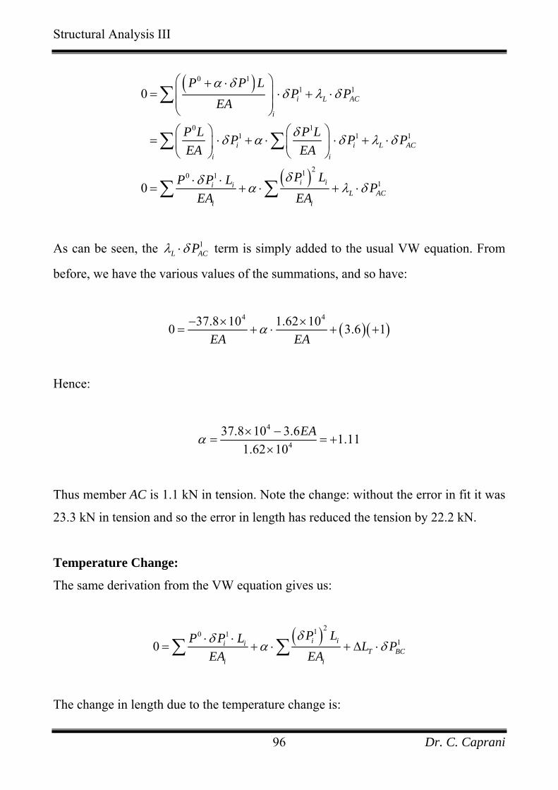
As can be seen, the 1L ACPλ δ⋅ term is simply added to the usual VW equation. From
before, we have the various values of the summations, and so have:
( )(4 437.8 10 1.62 100 3 ).6 1
EA EAα− × ×
= + ⋅ + +
Hence:
4
4
37.8 10 3.6 1.111.62 10
EAα × −= =
×+
Thus member AC is 1.1 kN in tension. Note the change: without the error in fit it was
23.3 kN in tension and so the error in length has reduced the tension by 22.2 kN.
Temperature Change:
The same derivation from the VW equation gives us:
( )210 110 i ii i
T Bi i
P LP P LCL P
EA EAδδ α δ⋅ ⋅
= + ⋅ + ∆∑ ∑ ⋅
The change in length due to the temperature change is:
Dr. C. Caprani 96

Structural Analysis III
( )( )( )(610 10 3000 50
1.5 mm
TL L Tα−
∆ = ∆
= × −
= −
)
Noting that the virtual force in member BC is , we have: 1 0.6BCPδ =
( )(4 437.8 10 1.62 100 1 ).5 0.6
EA EAα− × ×
= + ⋅ + −
Giving:
4
4
37.8 10 0.9 28.91.62 10
EAα × += =
×+
Thus member AC is 28.9 kN in tension an increase of 5.4 kN.
Error in Support Location:
Modifying the VW equation gives:
( )210 1i ii i
S Di i
P LP P LHEA EA
δδλ δ α⋅ ⋅⋅ = + ⋅∑ ∑
The value of the virtual horizontal reaction is found from the virtual force system to
be 0.6 kN to the right. Hence:
( )( )4 437.8 10 1.62 105 0.6
EA Eα− × ×
+ = + ⋅A
Dr. C. Caprani 97
Structural Analysis III
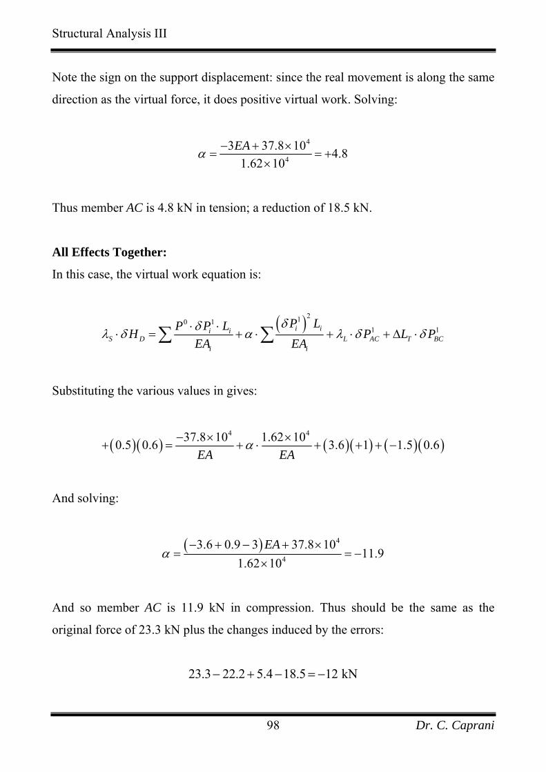
Note the sign on the support displacement: since the real movement is along the same
direction as the virtual force, it does positive virtual work. Solving:
4
4
3 37.8 10 4.81.62 10
EAα − + ×= =
×+
Thus member AC is 4.8 kN in tension; a reduction of 18.5 kN.
All Effects Together:
In this case, the virtual work equation is:
( )210 11 1i ii i
S D L AC Ti i
P LP P LBCH P L P
EA EAδδλ δ α λ δ δ⋅ ⋅
⋅ = + ⋅ + ⋅ + ∆ ⋅∑ ∑
Substituting the various values in gives:
( )( ) ( )( ) ( )(4 437.8 10 1.62 100.5 0.6 3.6 1 1.5 0.6)
EA EAα− × ×
+ = + ⋅ + + + −
And solving:
( ) 4
4
3.6 0.9 3 37.8 1011.9
1.62 10EA
α− + − + ×
= =×
−
And so member AC is 11.9 kN in compression. Thus should be the same as the
original force of 23.3 kN plus the changes induced by the errors:
23.3 22.2 5.4 18.5 12 kN− + − = −
Dr. C. Caprani 98
Structural Analysis III
6.3 Beams
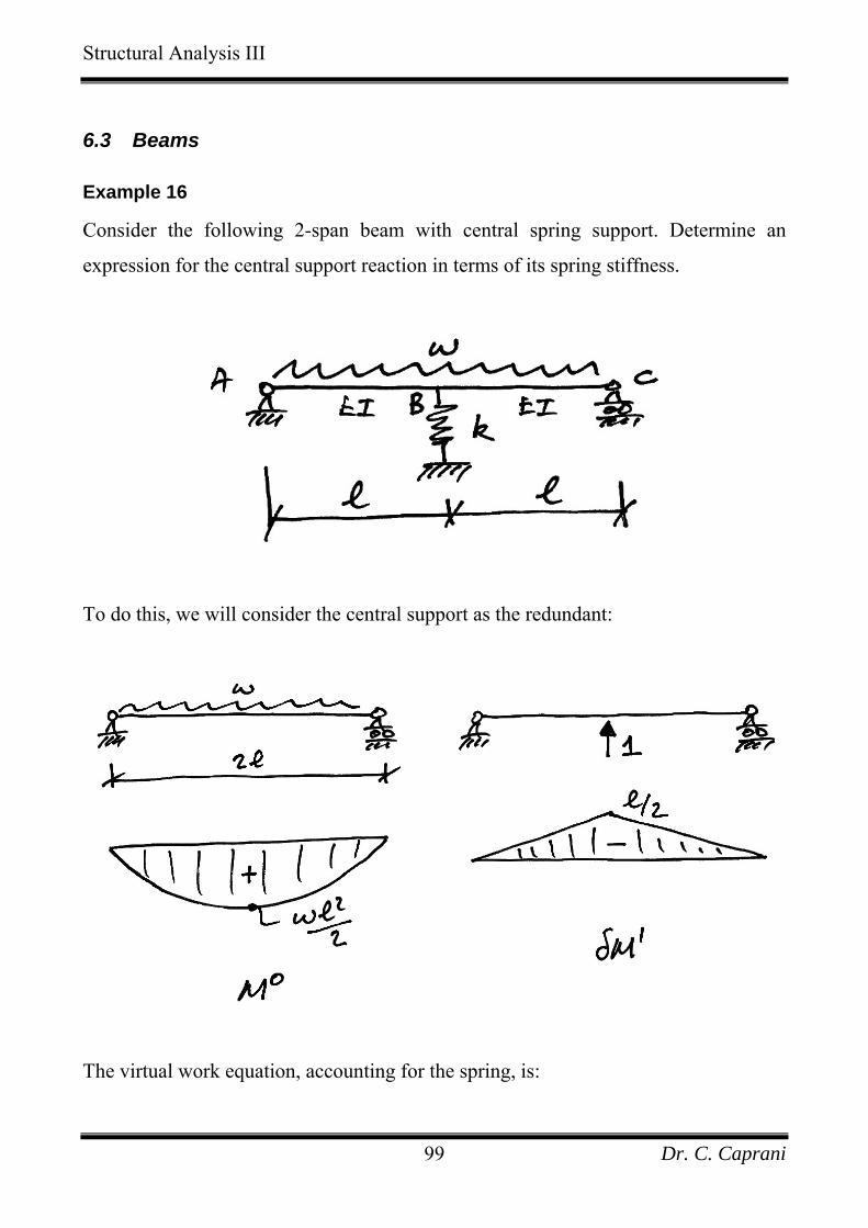
Example 16
Consider the following 2-span beam with central spring support. Determine an
expression for the central support reaction in terms of its spring stiffness.
To do this, we will consider the central support as the redundant:
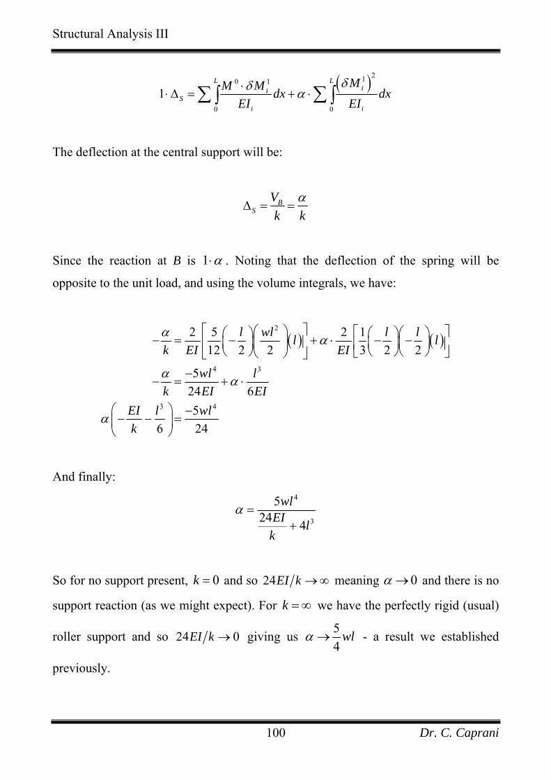
The virtual work equation, accounting for the spring, is:
Dr. C. Caprani 99
Structural Analysis III
( )210 1
0 0
1L L
iiS
i i
MM M dx dxEI EI
δδ α⋅⋅ ∆ = + ⋅∑ ∑∫ ∫
The deflection at the central support will be:
BS
Vk k
α∆ = =
Since the reaction at B is 1 α⋅ . Noting that the deflection of the spring will be
opposite to the unit load, and using the volume integrals, we have:
( ) ( )2
4 3
3 4
2 5 2 112 2 2 3 2 2
524 65
6 24
l wl l ll lk EI EI
wl lk EI EI
EI l wlk
α α
α α
α
⎡ ⎤⎛ ⎞ ⎡ ⎤⎛ ⎞ ⎛ ⎞⎛ ⎞− = − + ⋅ − −⎢ ⎥⎜ ⎟⎜ ⎟ ⎜ ⎟⎜ ⎟⎢ ⎥⎝ ⎠ ⎝ ⎠⎝ ⎠⎣ ⎦⎝ ⎠⎣ ⎦−
− = + ⋅
⎛ ⎞ −− − =⎜ ⎟⎝ ⎠
And finally: 4
3
524 4
wlEI l
k
α =+
So for no support present, and so 0k = 24EI k →∞ meaning 0α → and there is no
support reaction (as we might expect). For k = ∞ we have the perfectly rigid (usual)
roller support and so 24 0EI k → giving us 54
wlα → - a result we established
previously.
Dr. C. Caprani 100

Structural Analysis III
6.4 Frames
Example 17
The following frame, in addition to its loading, is subject to:
• Support A is located 10 mm too far to the left;
• End C of member BC is 31.2 10 rads−× out of square, as shown;
• Member CD is 12 mm too short.
Determine the bending moment diagram. Take EI = 36 × 103 kNm2 for each member.
We will choose the horizontal reaction at A as the redundant. Since we are dealing
with a linear lack of fit in member CD, we need to allow for the virtual work done by
the axial forces in this member and so we solve for the axial force diagrams also.
For the primary structure:
20 0
about 0 :
624 90 4 90 2 6 0 162 kN2 D D
M A
V V
=
⋅ + ⋅ + ⋅ − ⋅ = ∴ =
∑
Dr. C. Caprani 101
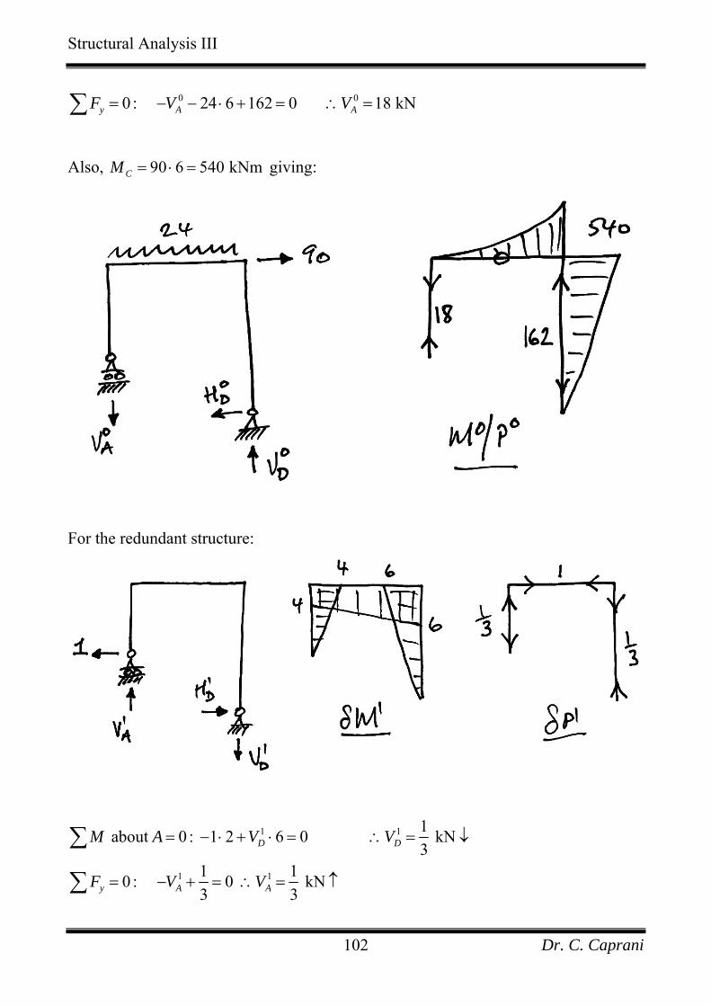
Structural Analysis III
0 00 : 24 6 162 0 18 kNy A AF V V= − − ⋅ + = ∴ =∑
Also, giving: 90 6 540 kNmCM = ⋅ =
For the redundant structure:
1 1
1 1
1 about 0 : 1 2 6 0 kN3
1 10 : 0 kN3 3
D D
y A A
M A V V
F V V
= − ⋅ + ⋅ = ∴ =
= − + = ∴ = ↑
∑
∑
↓
Dr. C. Caprani 102

Structural Analysis III
The virtual work equation, accounting for the relevant effects is:
( )210 11 1 1
0 0
0
E I
L Lii
S A C L Ci i
WW W
MM MDH dx dx M P
EI EI θ
δδ δ
δδλ α λ δ
==
⋅⋅ = + ⋅ + ⋅ + ⋅∑ ∑∫ ∫ λ δ
A
We take each term in turn:
(a) 1S Hλ ⋅ : The applied unit load is in the same direction as the error in the
support location, and keeping all units in metres:
( )1 3 310 10 1 10 10 kN mS AHλ − −⋅ = × ⋅ + = × ⋅
(b) 0 1
0
Li
i
M M dxEIδ⋅∑∫ : Using the volume integrals:
( )( ) ( )( )0 1
0
1 1 14 3 6 540 6 6 540 612 3
12420
Li
BC CDi
M M dxEI EI
EI
δ ⎧ ⎫⋅ ⎡ ⎤ ⎡= + ⋅ − + −⎨ ⎬⎢ ⎥ ⎢⎣ ⎦ ⎣⎩ ⎭
= −
∑∫ ⎤⎥⎦
(c) ( )21
0
Li
i
Mdx
EIδ
∑∫ : Again using the integrals table:
( ) ( )( ) ( ) ( )( )
( )( )
21
0
1 1 1 14 4 4 4 2 4 6 6 4 2 6 63 6
1 1 6 6 63
Li
AB Bi
CD
Mdx
EI EI EI
EI
δ ⎡ ⎤ ⎡= + ⋅ + + +⎢ ⎥ ⎢⎣ ⎦ ⎣
⎡ ⎤+ ⎢ ⎥⎣ ⎦
∑∫C
⎤⋅ ⎥⎦
Dr. C. Caprani 103

Structural Analysis III
( )21
0
245.33Li
i
Mdx
EI Eδ
=∑∫ I
(d) 1CMθλ δ⋅ : The virtual bending moment at C is 6 kNm with tension on the
inside of the frame. This is in the opposite direction to that needed to close the
lack of fit and so the sign of this term is negative, as shown:
( ) ( )1 3 31.2 10 6 7.2 10 kN mCMθλ δ − −⋅ = − × ⋅ = − × ⋅
(e) 1L CDPλ δ⋅ : Since the member is too short, the lack of fit is negative, whilst the
virtual force is in tension and so positive:
( ) ( )1 3 3112 10 4 10 kN m3L CDPλ δ − −⎛ ⎞⋅ = − × ⋅ + = − × ⋅⎜ ⎟
⎝ ⎠
Substituting these values into the equation, along with 336 10 kNm2EI = × , gives:
3 33 3
12420 245.3310 10 7.2 10 4 1036 10 36 10
α 3− − −× = − + ⋅ − × − ×× ×
Dr. C. Caprani 104

Structural Analysis III
And so we can solve for α :
10 345 6.815 7.2 410 345 7.2 4
6.81553.73
α
α
= − + ⋅ − −+ + +
=
=
And so the horizontal reaction at A is:
0 1 0 53.73 1 53.73 kNA A AH H Hα= + ⋅ = + ⋅ =
and similarly for the other reactions. Also, using the superposition equation for
moments, 0 1M M Mα= + ⋅ , we have:
Dr. C. Caprani 105
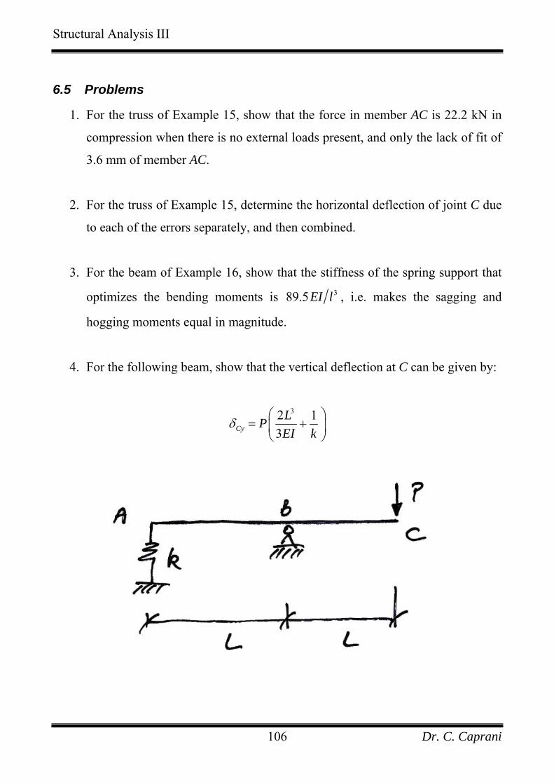
Structural Analysis III
6.5 Problems
1. For the truss of Example 15, show that the force in member AC is 22.2 kN in
compression when there is no external loads present, and only the lack of fit of
3.6 mm of member AC.
2. For the truss of Example 15, determine the horizontal deflection of joint C due
to each of the errors separately, and then combined.
3. For the beam of Example 16, show that the stiffness of the spring support that
optimizes the bending moments is 389.5EI l , i.e. makes the sagging and
hogging moments equal in magnitude.
4. For the following beam, show that the vertical deflection at C can be given by:
32 1
3CyLPEI k
δ⎛ ⎞
= +⎜ ⎟⎝ ⎠
Dr. C. Caprani 106
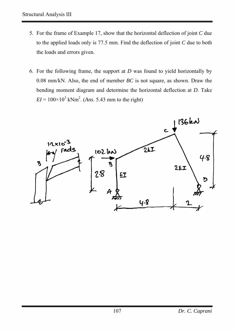
Structural Analysis III
5. For the frame of Example 17, show that the horizontal deflection of joint C due
to the applied loads only is 77.5 mm. Find the deflection of joint C due to both
the loads and errors given.
6. For the following frame, the support at D was found to yield horizontally by
0.08 mm/kN. Also, the end of member BC is not square, as shown. Draw the
bending moment diagram and determine the horizontal deflection at D. Take
EI = 100×103 kNm2. (Ans. 5.43 mm to the right)
Dr. C. Caprani 107
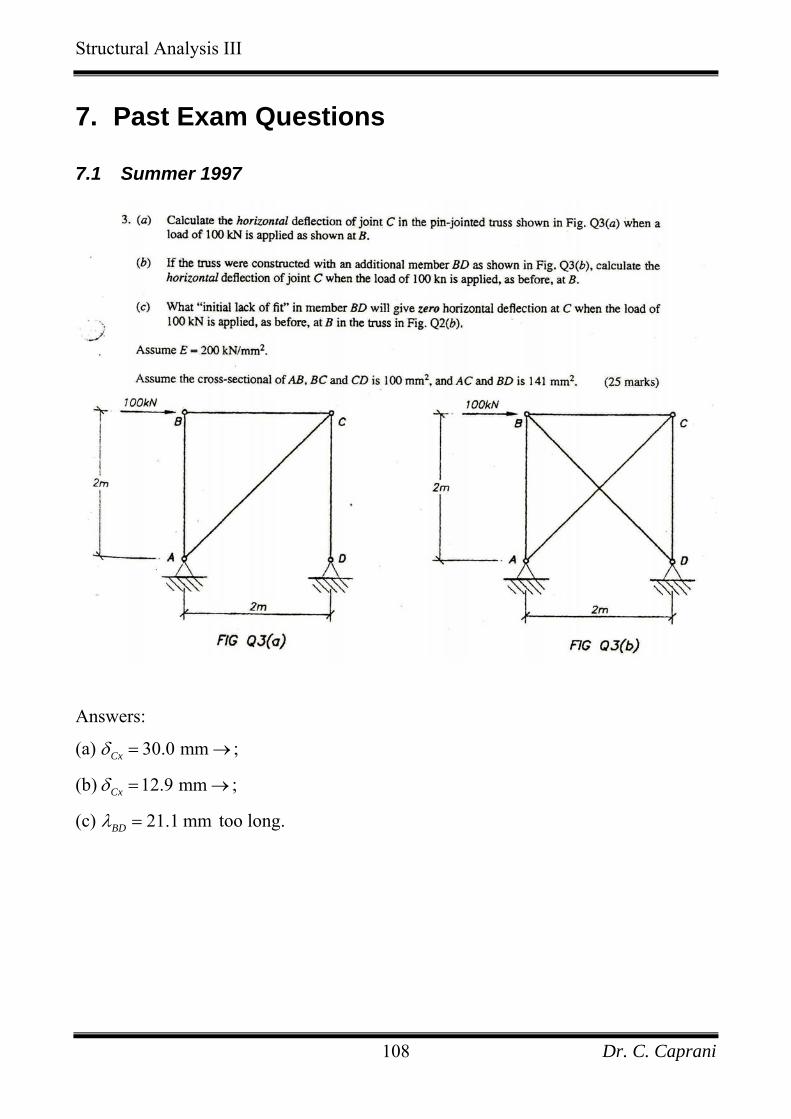
Structural Analysis III
7. Past Exam Questions
7.1 Summer 1997
Answers:
(a) 30.0 mmCxδ = → ;
(b) 12.9 mmCxδ = → ;
(c) 21.1 mmBDλ = too long.
Dr. C. Caprani 108

Structural Analysis III
7.2 Summer 1998
Answers:
(a) 45.0 mmCxδ = → ;
(b) 26.2 mmCxδ = → .
Dr. C. Caprani 109
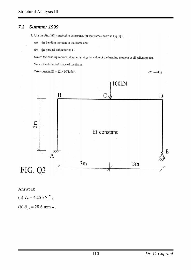
Structural Analysis III
7.3 Summer 1999
Answers:
(a) ; 42.5 kNEV = ↑
(b) . 28.6 mmCyδ = ↓
Dr. C. Caprani 110
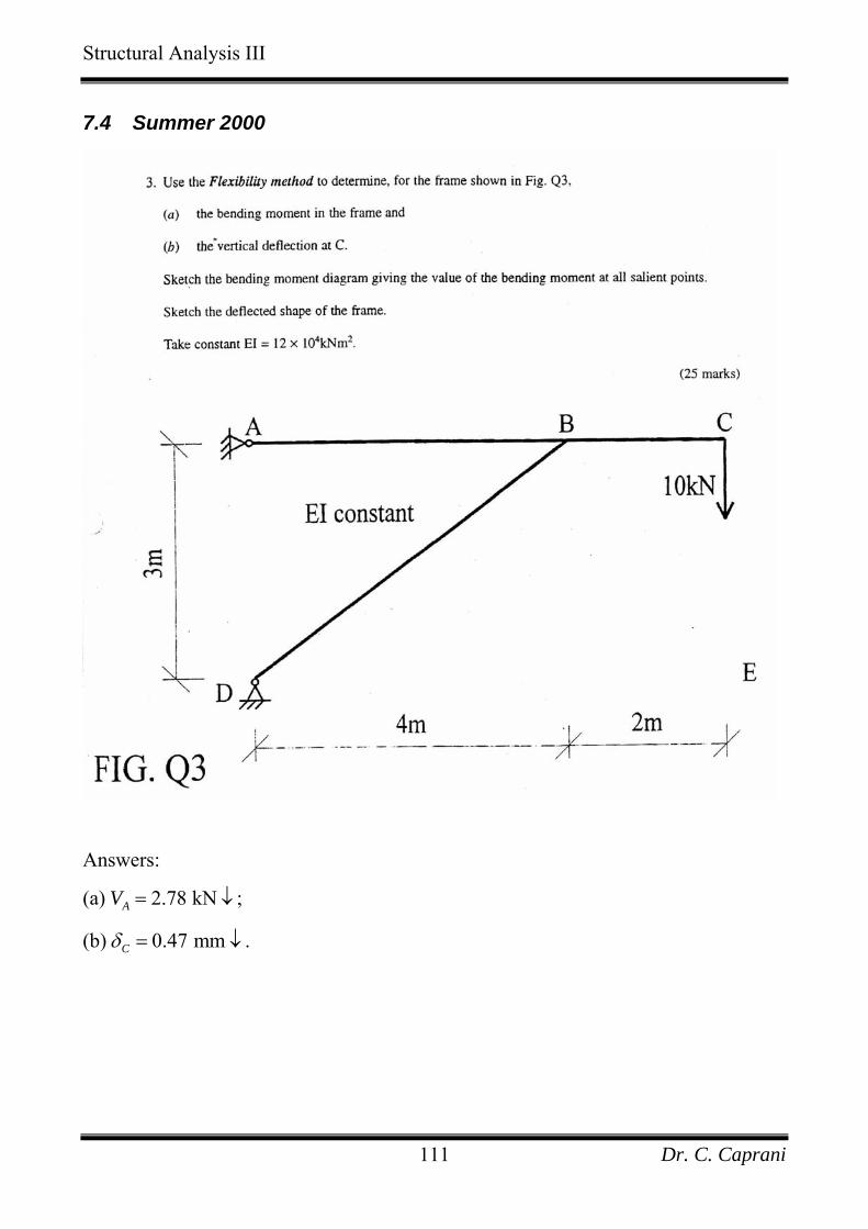
Structural Analysis III
7.4 Summer 2000
Answers:
(a) ; 2.78 kNAV = ↓
(b) . 0.47 mmCδ = ↓
Dr. C. Caprani 111
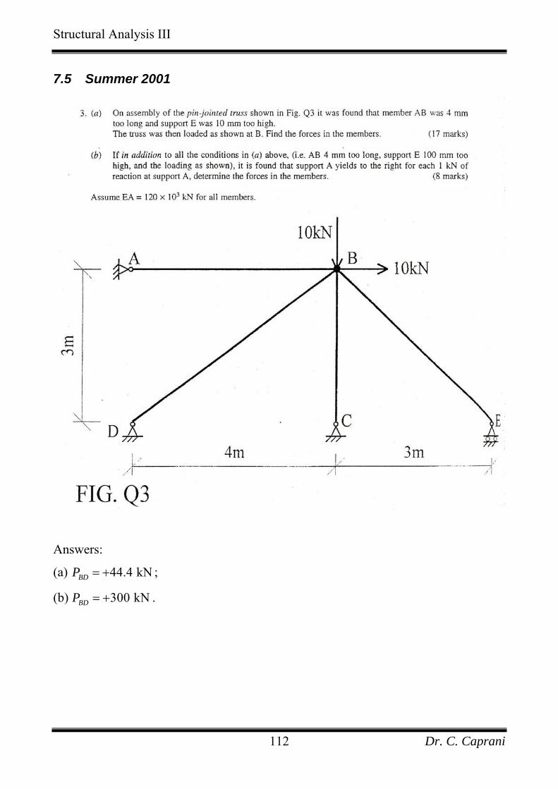
Structural Analysis III
7.5 Summer 2001
Answers:
(a) ; 44.4 kNBDP = +
(b) . 300 kNBDP = +
Dr. C. Caprani 112

Structural Analysis III
7.6 Summer 2002
Answers:
(a) 1.35 mmLλ = shorter;
(b) . 160 kNCV = ↑
Dr. C. Caprani 113
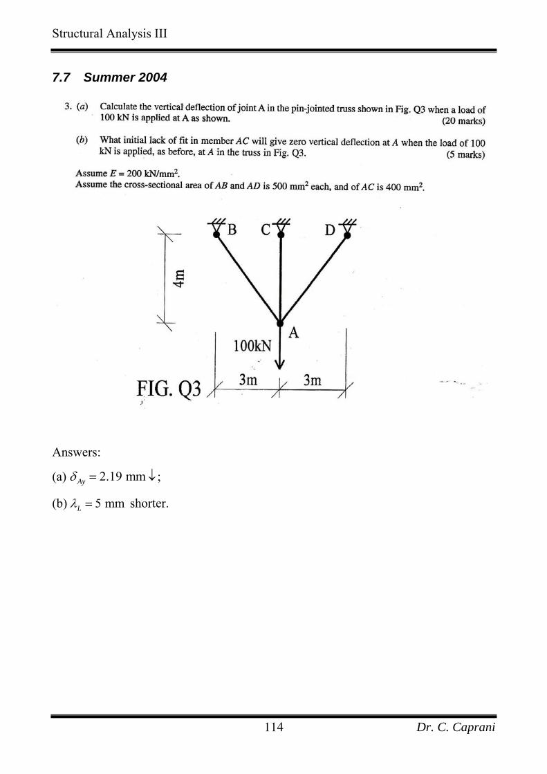
Structural Analysis III
7.7 Summer 2004
Answers:
(a) ; 2.19 mmAyδ = ↓
(b) 5 mmLλ = shorter.
Dr. C. Caprani 114

Structural Analysis III
7.8 Summer 2007 Using Virtual Work:
(i) For the frame in Fig. Q3(a), determine the horizontal deflection of joint C;
(ii) Draw the bending moment diagram for the frame in Fig. Q3(b);
(iii) Determine the horizontal deflection of joint C for the frame in Fig. Q3(b).
Note:
You may neglect axial effects in the members.
Take for all members. 336 10 kNmEI = × 2
FIG. Q3(a)
4 m
4 m
A
B C
20 k
N/m
100 kN
4 m
D
FIG. Q3(b)
4 m
4 m
A
B C
20 k
N/m
100 kN
4 m
D
Answers:
(a) 84.6 mmCxδ = → ;
(b) ; 75.8 kNDH = ←
(c) 19.02 mmCxδ = → .
Dr. C. Caprani 115
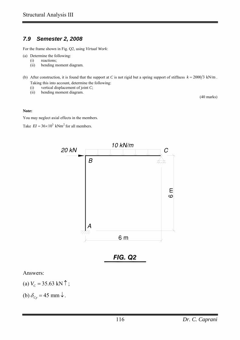
Structural Analysis III
7.9 Semester 2, 2008 For the frame shown in Fig. Q2, using Virtual Work:
(a) Determine the following: (i) reactions; (ii) bending moment diagram.
(b) After construction, it is found that the support at C is not rigid but a spring support of stiffness 2000 3 kN/mk = . Taking this into account, determine the following: (i) vertical displacement of joint C; (ii) bending moment diagram.
(40 marks)
Note:
You may neglect axial effects in the members.
Take for all members. 336 10 kNmEI = × 2
FIG. Q2
B
A
10 kN/mC
6 m
6 m
20 kN
Answers:
(a) ; 35.63 kNCV = ↑
(b) . 45 mmCyδ = ↓
Dr. C. Caprani 116
Structural Analysis III
8. References • Charlton, T.M., Analysis of Statically Indeterminate Frameworks, Longmans,
1961.
• Charlton, T.M., Energy Principles in Theory of Structures, Oxford University
Press, 1973.
• Coates, R.C., Coutie, M.G. and Kong, F.K., Structural Analysis, Chapman and
Hall, 1987.
• Davies, G.A.O., Virtual Work in Structural Analysis, John Wiley & Sons, 1982.
• Dym, C.L., Structural Modeling and Analysis, Cambridge University Press, 2005.
• Gregory, M.S., Introduction to Extremum Principles, Butterworths, London, 1969.
• Guarracino, F. and Walker, A., Energy Methods in Structural Mechanics, Thomas
Telford, 1999.
• Heyman, J., Beams and Framed Structures, 2nd Edn., Pergamon Press, 1974.
• Kong, F.K., Prentis, J.M. and Charlton, T.M., ‘Principle of virtual work for a
general deformable body – a simple proof’, The Structural Engineer, Vol. 61A,
No. 6, 1983.
• Neal, B.G., Structural Theorems and their Applications, Pergamon Press, 1964.
• Thompson, F. and Haywood, G.G., Structural Analysis Using Virtual Work,
Chapman and Hall, 1986.
• Rajasekaran, S. and Sankarasubramanian, G., Computational Structural
Mechanics, Prentis Hall of India, New Delhi, 2001.
• Richards, T.H., Energy methods in Stress Analysis, Ellis Horwood, 1977.
• Wallerstein, D.V. , A Variational Approach to Structural Analysis, Wiley, 2001.
Dr. C. Caprani 117
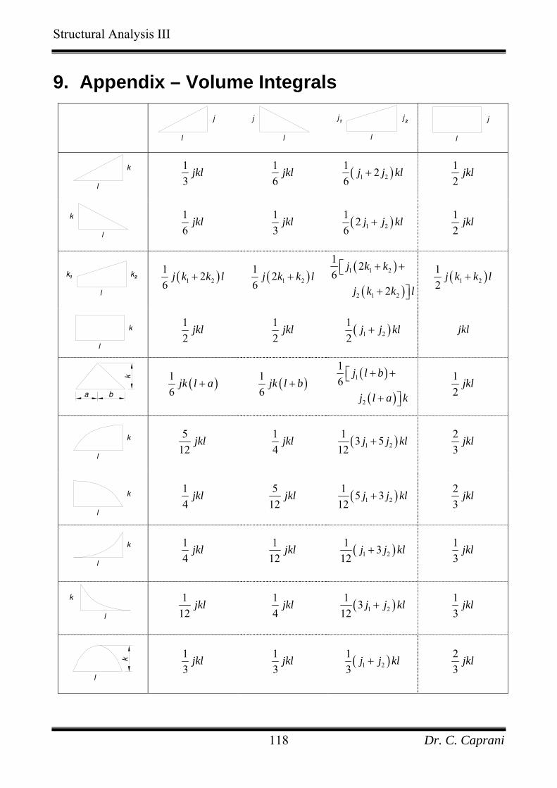
Structural Analysis III
9. Appendix – Volume Integrals
l
j
l
j
l
jj1 2
l
j
l
k
13
jkl 16
jkl ( )1 21 26
j j+ kl 12
jkl
l
k
16
jkl 13
jkl ( )1 21 26
j j kl+ 12
jkl
l
kk1 2
( )1 2
1 26
j k k+ l ( )1 21 26
j k k+ l ( )
( )
1 1 2
2 1 2
1 26
2
j k k
j k k l
+ +⎡⎣
+ ⎤⎦
( )1 212
j k k+ l
l
k
12
jkl 12
jkl ( )1 212
j j k+ l jkl
a b
k
( )16
jk l a+ ( )16
jk l b+ ( )
( )
1
2
16
j l b
j l a k
+ +⎡⎣
+ ⎤⎦
12
jkl
l
k
512
jkl 14
jkl ( )1 21 3 5
12j j kl+ 2
3jkl
l
k
14
jkl 512
jkl ( )1 21 5 3
12j j+ kl 2
3jkl
l
k
14
jkl 112
jkl ( )1 21 3
12j j kl+ 1
3jkl
l
k
112
jkl 14
jkl ( )1 21 3
12j j kl+ 1
3jkl
k
l
13
jkl 13
jkl ( )1 213
j j kl+ 23
jkl
Dr. C. Caprani 118