
Aero 306 Structural Analysis II “Introduction to Classical Virtual Work
112
C:\W\whit\Classes\306\Notes\1_Intro_and_ClassicalVW\0_Introduction&Review\1_introduction.docx p. 1 Aero 306 Structural Analysis II “Introduction to Classical Virtual Work and Finite Elements” John Whitcomb ©2010
Transcript of Aero 306 Structural Analysis II “Introduction to Classical Virtual Work


C:\W\whit\Classes\306\Notes\1_Intro_and_ClassicalVW\0_Introduction&Review\2_syllabus.docx p. 3 of
papers, and other academic work. Ignorance of the rules does not exclude any member of the Texas
A&M University community from the requirements or the processes of the Honor System. For additional
information please visit: www.tamu.edu/aggiehonor/
On all course work, assignments, and examinations at Texas A&M University, the following Honor Pledge
shall be preprinted and signed by the student: “On my honor, as an Aggie, I have neither given nor
received unauthorized aid on this academic work.”
Contributions to Professional Component:
1. Provides foundation for computer analysis of structures using finite elements. 2. Provides experience in design process through team project. 3. Provides experience in teaming.
Relationship to program Outcomes:
Objective Assessment Method ABET
Outcome
Understand that many structural analysis problems cannot be solved
exactly, but there are systematic, reliable strategies for obtaining
approximate solutions.
Homework, Major
Exams, Final Exam
3a, 3e
Understand that virtual work is a powerful alternative to summing
forces or solving differential equations to obtain equilibrium states.
Homework, Major
Exams, Final Exam
3a, 3e
Understand the requirements for valid assumed solutions and how
to solve for the unknown coefficients.
Homework, Major
Exams, Final Exam
3a, 3e
Understand the convergence behavior of energy methods.
Homework, Major
Exams, Final Exam
3a, 3e
Understand the application of energy principles for uniaxial
rods, beams, trusses, and frames.
Homework, Major
Exams, Final Exam
3a, 3e
Understand theoretical basis for finite elements.
Homework, Major
Exams, Final Exam
3a, 3e
Understand how to write a finite element code for beam
analysis.
Write a finite element
code
3a, 3e
1/3/2012 p. 7 of 112

C:\W\whit\Classes\306\Notes\1_Intro_and_ClassicalVW\0_Introduction&Review\2_syllabus.docx p. 4 of
Understand the formulation of the buckling problem using
energy principles.
Homework, Major
Exams, Final Exam
3a, 3e
Understand how to use finite elements to optimize the
design of 2D structures.
Design project 3a, 3e, 3g, 3k
Understand how to work in teams to develop an optimal
design.
Design project 3f, 3g
1/3/2012 p. 8 of 112

C:\W\whit\Classes\306\Notes\1_Intro_and_ClassicalVW\0_Introduction&Review\3_review.docx p. 1 of 9
Review of Some Basic Concepts Review your 214 and 304 notes. Classification of governing equations for structural analysis
Equilibrium equations
“Constitutive” equations
Kinematic equations
Boundary conditions There are always assumptions, even in full three dimensional analysis (Remember those partial differential equations that you saw & could not solve? They are still only an approximation!) Classification of concepts, assumptions, and resulting equations for structural analysis
Let’s review this for uniaxial bars (Remember 0d du
EA fdx dx
)
We will flesh this out in class. Be sure to take good notes. In each group, there are assumptions that result in great simplification… what are the assumptions?
Equilibrium o Stresses? o Forces? (Stress resultants) o Requirement(s) for equilibrium
“Constitutive” o Stress vs strain o Relationship between force and strain due to simplified kinematics
Kinematic o Displacements (variation?) o Deformation vs displacements
Boundary conditions o What is the boundary? o Types of BC’s
Force Displacement
o Relationship between internal force and applied force
You might repeat this summary for beam analysis as HW assignment. Let’s perform full 3D analysis of the following “beam-like” structure.
1/3/2012 p. 9 of 112
C:\W\whit\Classes\306\Notes\1_Intro_and_ClassicalVW\0_Introduction&Review\3_review.docx p. 2 of 9
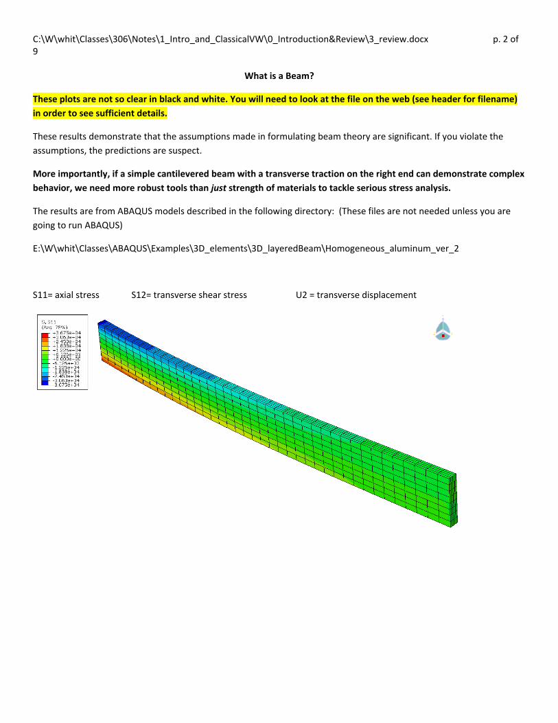
What is a Beam?
These plots are not so clear in black and white. You will need to look at the file on the web (see header for filename)
in order to see sufficient details.
These results demonstrate that the assumptions made in formulating beam theory are significant. If you violate the
assumptions, the predictions are suspect.
More importantly, if a simple cantilevered beam with a transverse traction on the right end can demonstrate complex
behavior, we need more robust tools than just strength of materials to tackle serious stress analysis.
The results are from ABAQUS models described in the following directory: (These files are not needed unless you are
going to run ABAQUS)
E:\W\whit\Classes\ABAQUS\Examples\3D_elements\3D_layeredBeam\Homogeneous_aluminum_ver_2
S11= axial stress S12= transverse shear stress U2 = transverse displacement
1/3/2012 p. 10 of 112

C:\W\whit\Classes\306\Notes\1_Intro_and_ClassicalVW\0_Introduction&Review\3_review.docx p. 3 of 9
Because of stress concentrations at the support (not predictable from beam theory), we need to manually adjust the
limits for the contour plot. If you stay away from the ends, I think you will find that beam theory predicts the transverse
shear stress quite well.
1/3/2012 p. 11 of 112

C:\W\whit\Classes\306\Notes\1_Intro_and_ClassicalVW\0_Introduction&Review\3_review.docx p. 4 of 9
Now we will analyze a beam with a square cross section. Does this structure behave like a beam?
From a quick look it seems that the axial stress is probably varying pretty much like a simple beam, but not so for the
transverse shear stress.
1/3/2012 p. 12 of 112
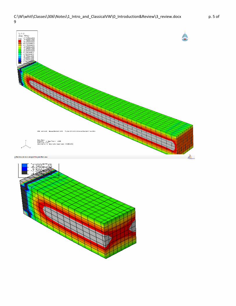
C:\W\whit\Classes\306\Notes\1_Intro_and_ClassicalVW\0_Introduction&Review\3_review.docx p. 5 of 9
1/3/2012 p. 13 of 112
C:\W\whit\Classes\306\Notes\1_Intro_and_ClassicalVW\0_Introduction&Review\3_review.docx p. 6 of 9
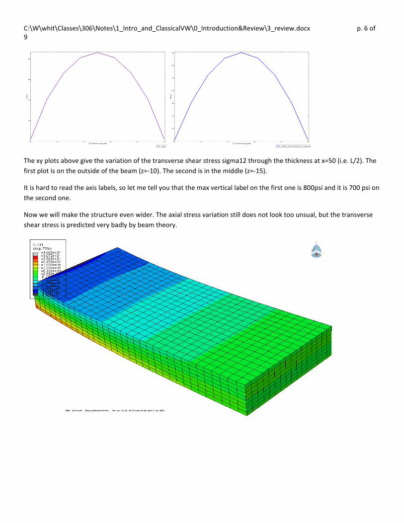
The xy plots above give the variation of the transverse shear stress sigma12 through the thickness at x=50 (i.e. L/2). The
first plot is on the outside of the beam (z=‐10). The second is in the middle (z=‐15).
It is hard to read the axis labels, so let me tell you that the max vertical label on the first one is 800psi and it is 700 psi on
the second one.
Now we will make the structure even wider. The axial stress variation still does not look too unsual, but the transverse
shear stress is predicted very badly by beam theory.
1/3/2012 p. 14 of 112

C:\W\whit\Classes\306\Notes\1_Intro_and_ClassicalVW\0_Introduction&Review\3_review.docx p. 7 of 9
1/3/2012 p. 15 of 112

C:\W\whit\Classes\306\Notes\1_Intro_and_ClassicalVW\0_Introduction&Review\3_review.docx p. 8 of 9
The deformation is anticlastic. Why?
This is a contour plot of the transverse displacement.
Anticlastic: “Having the property of a surface or portion of a surface whose two principal curvatures at each point have
opposite signs, so that one normal section is concave and the other convex.” http://www.answers.com/topic/anticlastic‐
mathematics
1/3/2012 p. 16 of 112

C:\W\whit\Classes\306\Notes\1_Intro_and_ClassicalVW\0_Introduction&Review\3_review.docx p. 9 of 9
1/3/2012 p. 17 of 112

C:\W\whit\Classes\306\Notes\1_Intro_and_ClassicalVW\1_VirtualWork_mechanisms\1_VW_introduction.doc p. 1 of 17
Introduction to
Virtual Work
Equilibrium Equations that Do Not Set Sum of Forces = 0!
Introductory Problems: Mechanisms
1/3/2012 p. 18 of 112
C:\W\whit\Classes\306\Notes\1_Intro_and_ClassicalVW\1_VirtualWork_mechanisms\1_VW_introduction.doc p. 2 of 17
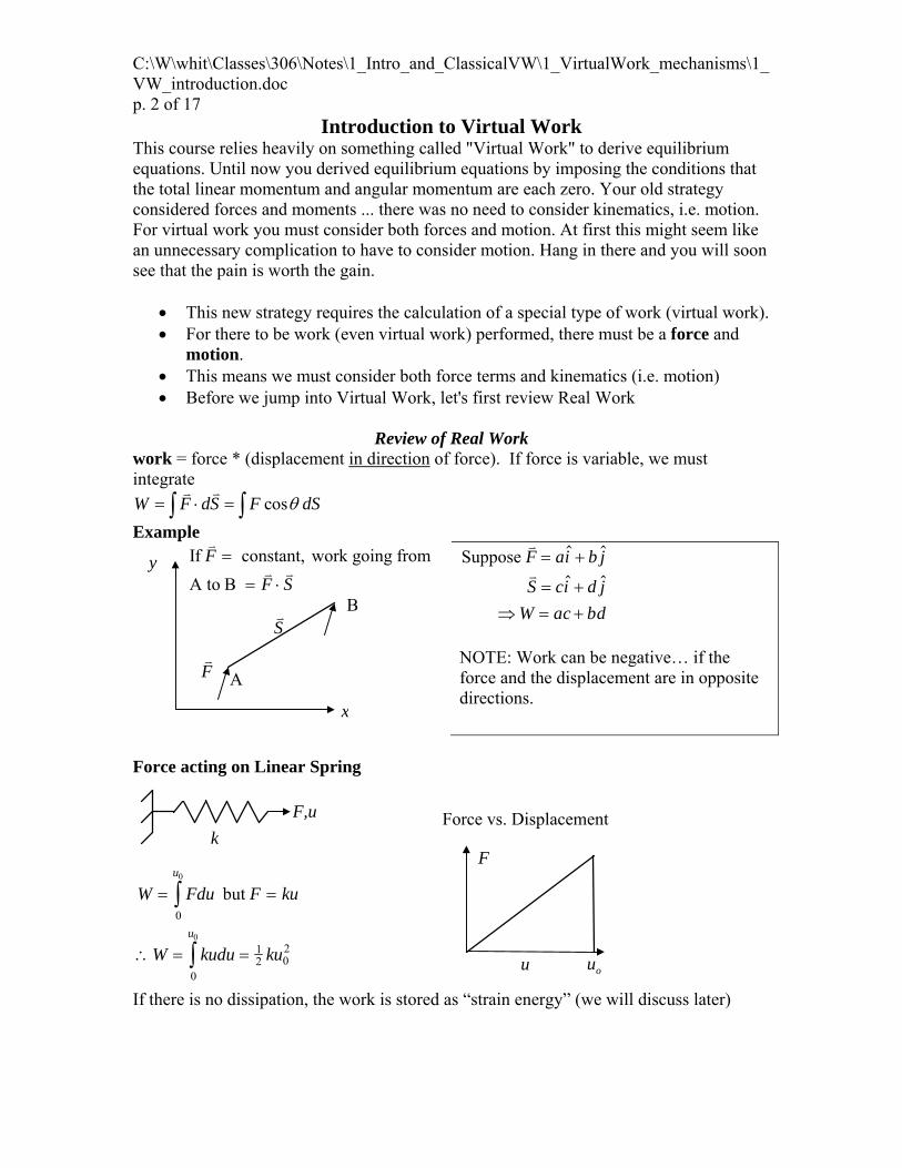
Introduction to Virtual Work This course relies heavily on something called "Virtual Work" to derive equilibrium equations. Until now you derived equilibrium equations by imposing the conditions that the total linear momentum and angular momentum are each zero. Your old strategy considered forces and moments ... there was no need to consider kinematics, i.e. motion. For virtual work you must consider both forces and motion. At first this might seem like an unnecessary complication to have to consider motion. Hang in there and you will soon see that the pain is worth the gain.
This new strategy requires the calculation of a special type of work (virtual work). For there to be work (even virtual work) performed, there must be a force and
motion. This means we must consider both force terms and kinematics (i.e. motion) Before we jump into Virtual Work, let's first review Real Work
Review of Real Work
work = force * (displacement in direction of force). If force is variable, we must integrate
cosW F dS F dS
Example y
x
B
A F
S
If constant, work going from
A to B
F
F S
Suppose
F ai b j
S ci d j
W ac bd
NOTE: Work can be negative… if the force and the displacement are in opposite directions.
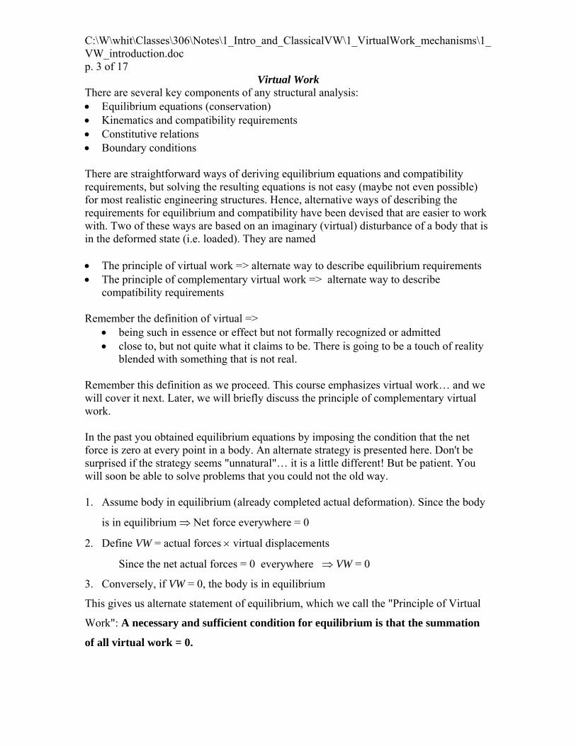
Force acting on Linear Spring
F
u uo
W Fdu F ku
W kudu ku
u
u
0
12 0
2
0
0
0
but
k
F,u Force vs. Displacement
If there is no dissipation, the work is stored as “strain energy” (we will discuss later)
1/3/2012 p. 19 of 112
C:\W\whit\Classes\306\Notes\1_Intro_and_ClassicalVW\1_VirtualWork_mechanisms\1_VW_introduction.doc p. 3 of 17
Virtual Work There are several key components of any structural analysis: Equilibrium equations (conservation) Kinematics and compatibility requirements Constitutive relations Boundary conditions There are straightforward ways of deriving equilibrium equations and compatibility requirements, but solving the resulting equations is not easy (maybe not even possible) for most realistic engineering structures. Hence, alternative ways of describing the requirements for equilibrium and compatibility have been devised that are easier to work with. Two of these ways are based on an imaginary (virtual) disturbance of a body that is in the deformed state (i.e. loaded). They are named The principle of virtual work => alternate way to describe equilibrium requirements The principle of complementary virtual work => alternate way to describe
compatibility requirements Remember the definition of virtual =>
being such in essence or effect but not formally recognized or admitted close to, but not quite what it claims to be. There is going to be a touch of reality
blended with something that is not real. Remember this definition as we proceed. This course emphasizes virtual work… and we will cover it next. Later, we will briefly discuss the principle of complementary virtual work. In the past you obtained equilibrium equations by imposing the condition that the net force is zero at every point in a body. An alternate strategy is presented here. Don't be surprised if the strategy seems "unnatural"… it is a little different! But be patient. You will soon be able to solve problems that you could not the old way. 1. Assume body in equilibrium (already completed actual deformation). Since the body
is in equilibrium Net force everywhere = 0
2. Define VW = actual forces virtual displacements
Since the net actual forces = 0 everywhere VW = 0
3. Conversely, if VW = 0, the body is in equilibrium
This gives us alternate statement of equilibrium, which we call the "Principle of Virtual
Work": A necessary and sufficient condition for equilibrium is that the summation
of all virtual work = 0.
1/3/2012 p. 20 of 112
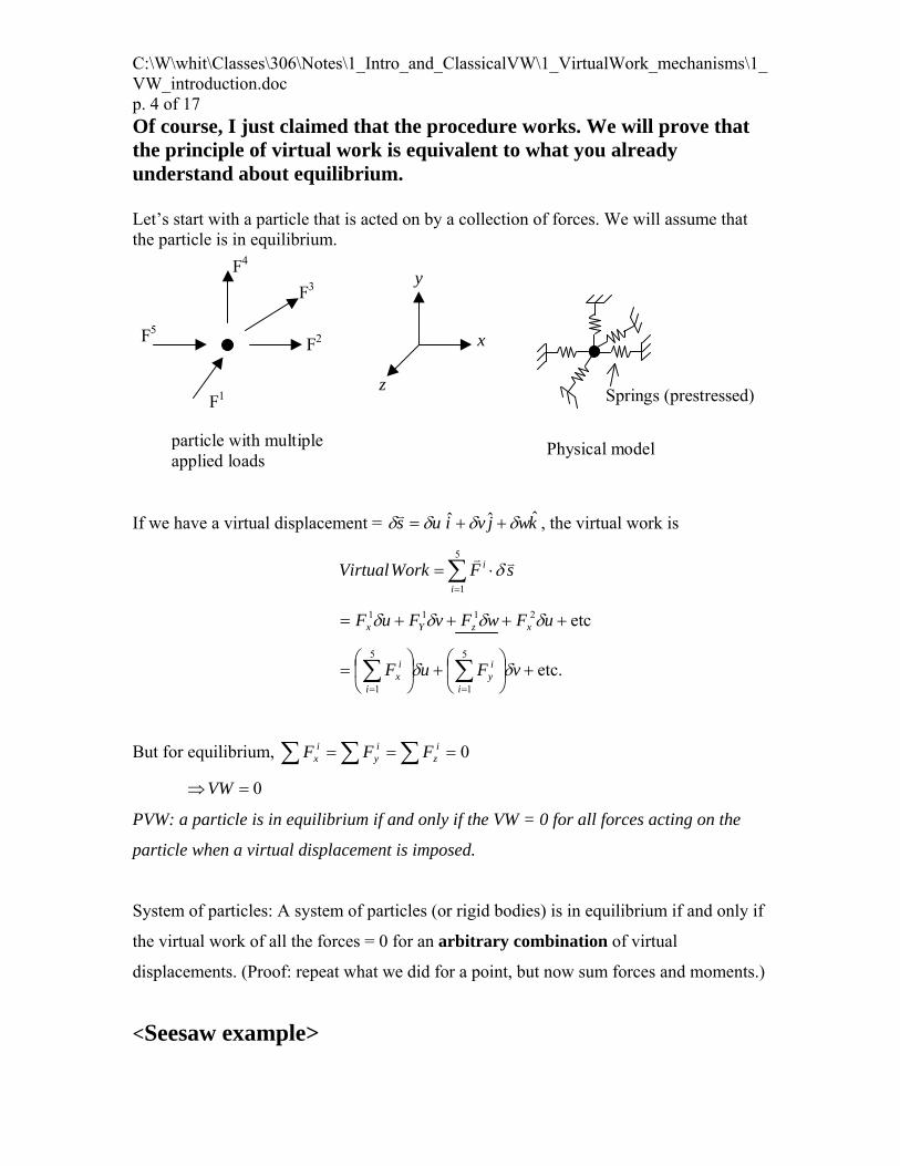
C:\W\whit\Classes\306\Notes\1_Intro_and_ClassicalVW\1_VirtualWork_mechanisms\1_VW_introduction.doc p. 4 of 17 Of course, I just claimed that the procedure works. We will prove that the principle of virtual work is equivalent to what you already understand about equilibrium. Let’s start with a particle that is acted on by a collection of forces. We will assume that the particle is in equilibrium.
Springs (prestressed)
particle with multipleapplied loads
Physical model
F4
F3
F2
F1
F5
z
x
y
If we have a virtual displacement = kwjvius ˆˆˆ , the virtual work is
5
1
i
i
VirtualWork F s
etc.
etc
5
1
5
1
2111
vFuF
uFwFvFuF
i
iy
i
ix
xzYx
But for equilibrium, 0iz
iy
ix FFF
0VW
PVW: a particle is in equilibrium if and only if the VW = 0 for all forces acting on the
particle when a virtual displacement is imposed.
System of particles: A system of particles (or rigid bodies) is in equilibrium if and only if
the virtual work of all the forces = 0 for an arbitrary combination of virtual
displacements. (Proof: repeat what we did for a point, but now sum forces and moments.)
<Seesaw example>
1/3/2012 p. 21 of 112

C:\W\whit\Classes\306\Notes\1_Intro_and_ClassicalVW\1_VirtualWork_mechanisms\1_VW_introduction.doc p. 5 of 17
Virtual Work versus Complementary Virtual Work In Aero 306 we will concentrate on Virtual Work. There is also a Complementary Virtual Work principle that was of more use before computers were invented. We will not go into details, but here is a brief comparison of the principles. Characteristics of the principle of virtual work Use to obtain equilibrium equations Virtual Work = actual forces at equilibrium * virtual displacement Virtual displacement = very small arbitrary change in displacements Virtual displacements must satisfy kinematic constraints Wherever displacements are specified, the virtual displacements must be zero.
Otherwise, the behavior would not be consistent with the kinematic constraints. Compatibility requirements must be satisfied exactly. The principle of complementary virtual work (optional) Use to obtain compatibility equations Complementary Virtual Work = actual displacements at equilibrium * virtual forces Virtual forces = very small change in the equilibrium forces Virtual forces must satisfy equilibrium requirements exactly=>
Internal forces are balanced exactly by applied forces at the boundaries Virtual forces = 0 where forces are specified Equilibrium is satisfied at every point inside the body
Before the advent of computers, the principle of complementary virtual work was quite popular. This was because many structures could be analyzed using a combination of experimental measurements and a few equations… or statics and a few equations. The principle of virtual work typically requires many equations, but has many advantages that will eventually become apparent. Now that computers allow the solution of thousands of equations very quickly, virtual work has become by far the preferred principle.
Summary of Using Virtual Work 1. Identify system. 2. Assume system (body) is in a deformed, equilibrium state. 3. Identify the active forces (forces that move) and label the conjugate displacements 4. Express position of active forces in terms of the displacements. (kinematics) 5. Use the expressions from step 4 to impose the virtual displacements (ie. changes in
the DOF). 6. Calculate the virtual work 7. Select DOF and impose constraints between the displacements 8. Solve: VW = 0 to obtain the values of the DOF.
1/3/2012 p. 22 of 112
C:\W\whit\Classes\306\Notes\1_Intro_and_ClassicalVW\1_VirtualWork_mechanisms\1_VW_introduction.doc p. 6 of 17 *Degrees of freedom = independent set of parameters which uniquely (completely) defines displacements at all points in a body. There are usually many possible sets. Choose the one that simplifies the analysis.
1/3/2012 p. 23 of 112

C:\W\whit\Classes\306\Notes\1_Intro_and_ClassicalVW\1_VirtualWork_mechanisms\1_VW_introduction.doc p. 7 of 17
Analysis of a Spring Using Virtual Work We must consider three states:
Original state (before applying load) Deformed state Deformed state + virtual displacement
As we go through this example, note how each state is used. Since we do not know how to calculate the virtual work for a spring, we will replace the original system with an equivalent one that has no spring.
F
K
u
Q=Ku
F
Original Configuration Equivalent Configuration
System = particle
Spring is stretched and Q Ku
dof = u
active forces = Q and F
Impose virtual displacement u
Calculate virtual work and set =0 to obtain equilibrium equation
VW F u Q u 0
0
0
( ) 0
Solve to obtain u=F/K
VW F u Q u
F u Ku u
u F Ku
F Ku
1/3/2012 p. 24 of 112


C:\W\whit\Classes\306\Notes\1_Intro_and_ClassicalVW\1_VirtualWork_mechanisms\1_VW_introduction.doc p. 12 of 17
Application of VW Equation: Hard Way & Easy Way When the kinematics are not trivial, it is useful to understand something called the “variational operator”. We will now describe what it is and illustrate why it is useful.
P, u
a
M
Inextensible bar of length L
Suppose the current equilibrium state is as shown
0
0
a a u
0
0
where initial valueof u=translation in direction of P
a initial valueof a α=rotation in direction of
Now impose virtual displacements ,u
VW P u M 0 This is the virtual work, but u and are not independent. To proceed further we must find the relationship between u and . If we assume the bar is inextensible and it's length = L, then simple trigonometry will give us a relationship between andu .
00
a u ucos
L
This can be simplified by recognizing that u and are infinitesimal.
1 2 1 2 1 2
0 0 0
Recall the formula: cos( ) cos cos sin sin
cos( ) cos( )cos( ) sin( )sin( )
But is extremelysmall sin cos 1and
00 0 0
00
0
a u ucos( ) cos( ) sin( )
La u
but cos( )L
sin( )
Therefore
u L
Now substitute this relationship into the expression for VW and solve to obtain M PLsin
1/3/2012 p. 29 of 112
C:\W\whit\Classes\306\Notes\1_Intro_and_ClassicalVW\1_VirtualWork_mechanisms\1_VW_introduction.doc p. 13 of 17
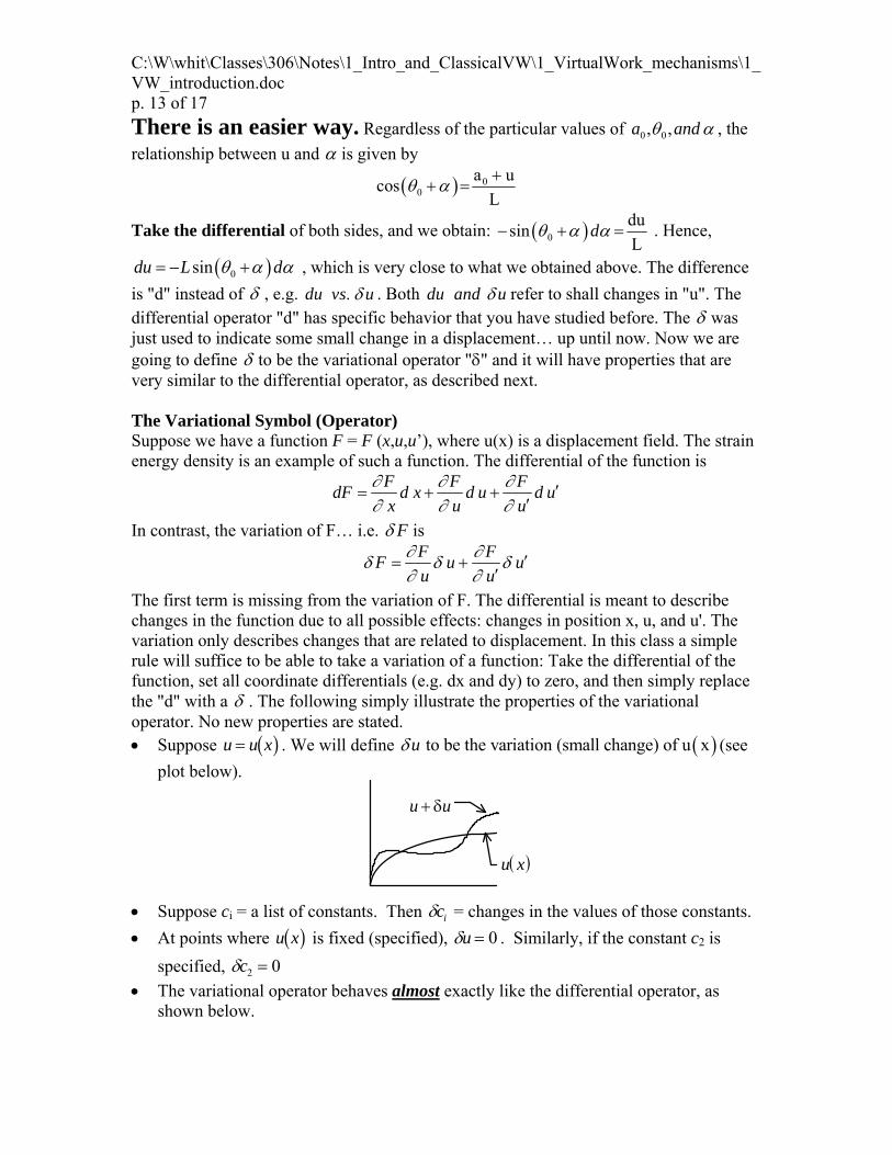
There is an easier way. Regardless of the particular values of 0 0, ,a and , the
relationship between u and is given by
00
a ucos
L
Take the differential of both sides, and we obtain: 0
dusin
Ld . Hence,
0sindu L d , which is very close to what we obtained above. The difference
is "d" instead of , e.g. .du vs u . Both du and u refer to shall changes in "u". The differential operator "d" has specific behavior that you have studied before. The was just used to indicate some small change in a displacement… up until now. Now we are going to define to be the variational operator "" and it will have properties that are very similar to the differential operator, as described next. The Variational Symbol (Operator) Suppose we have a function F = F (x,u,u’), where u(x) is a displacement field. The strain energy density is an example of such a function. The differential of the function is
F F FdF d x d u d u
x u u
In contrast, the variation of F… i.e. F is F F
F u uu u
The first term is missing from the variation of F. The differential is meant to describe changes in the function due to all possible effects: changes in position x, u, and u'. The variation only describes changes that are related to displacement. In this class a simple rule will suffice to be able to take a variation of a function: Take the differential of the function, set all coordinate differentials (e.g. dx and dy) to zero, and then simply replace the "d" with a . The following simply illustrate the properties of the variational operator. No new properties are stated. Suppose u u x b g . We will define to be the variation (small change) of u xu (see
plot below).
u u
u x
Suppose ci = a list of constants. Then ci = changes in the values of those constants.
At points where u xb g is fixed (specified), u 0 . Similarly, if the constant c2 is
specified, c2 0
The variational operator behaves almost exactly like the differential operator, as shown below.
1/3/2012 p. 30 of 112
C:\W\whit\Classes\306\Notes\1_Intro_and_ClassicalVW\1_VirtualWork_mechanisms\1_VW_introduction.doc p. 14 of 17
uv u v v u
u v u v
u n u u
d dx u du dx
udx udx
n n
a
b
a
b
b gb gd ib g b g
zz
1
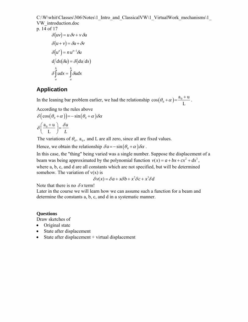
Application
In the leaning bar problem earlier, we had the relationship 00
a ucos
L
.
According to the rules above
0 0
0
0 0
cos sin
a u
L
The variations of , a , and L are all zero, since all are fixed values.
u
L
Hence, we obtain the relationship 0sinu .
In this case, the "thing" being varied was a single number. Suppose the displacement of a beam was being approximated by the polynomial function 2 3( )v x a bx cx dx , where a, b, c, and d are all constants which are not specified, but will be determined somehow. The variation of v(x) is
2 3( )v x a x b x c x d Note that there is no x term! Later in the course we will learn how we can assume such a function for a beam and determine the constants a, b, c, and d in a systematic manner. Questions Draw sketches of Original state State after displacement State after displacement + virtual displacement
1/3/2012 p. 31 of 112

C:\W\whit\Classes\306\Notes\1_Intro_and_ClassicalVW\1_VirtualWork_mechanisms\1_VW_introduction.doc p. 15 of 17 Try out what you have learned on this problem.
This time assume the spring is unstretched when theta = 30 degrees.
u = displacement of point A to the right.
This problem is studied in detail in the Collection of Mechanism Examples”.
Here is the basic strategy for analyzing mechanisms:
Define parameters that identify
Initial state
Undeformed state for any springs
Equilibrium state
Note that not all the parameters will be independent
Use kinematic constraints to express all of the parameters in terms of the
minimum set of dof.
Express the Virtual Work in terms of the dof
Set VW=0 to obtain the unknowns
1/3/2012 p. 32 of 112
C:\W\whit\Classes\306\Notes\1_Intro_and_ClassicalVW\1_VirtualWork_mechanisms\1_VW_introduction.doc p. 16 of 17
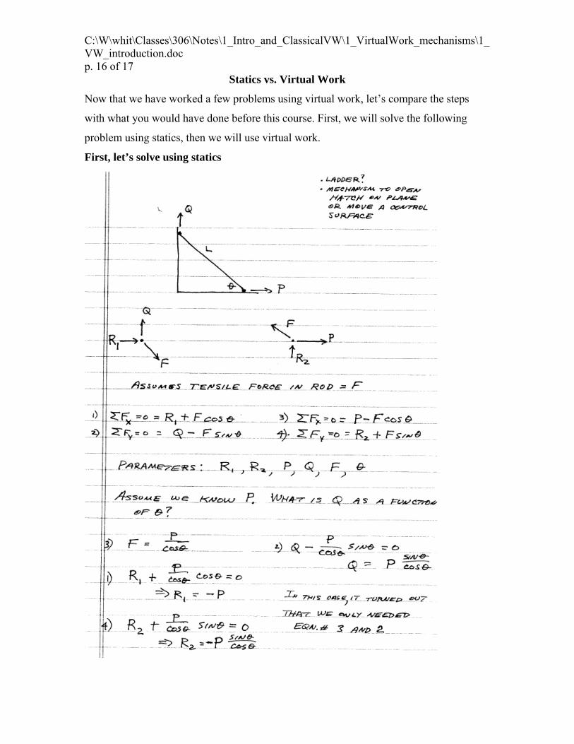
Statics vs. Virtual Work
Now that we have worked a few problems using virtual work, let’s compare the steps
with what you would have done before this course. First, we will solve the following
problem using statics, then we will use virtual work.
First, let’s solve using statics
1/3/2012 p. 33 of 112
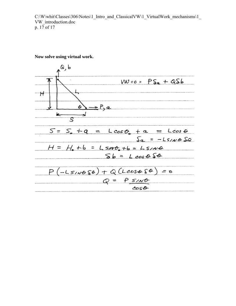
C:\W\whit\Classes\306\Notes\1_Intro_and_ClassicalVW\1_VirtualWork_mechanisms\1_VW_introduction.doc p. 17 of 17
Now solve using virtual work.
1/3/2012 p. 34 of 112

C:\W\whit\Classes\306\Notes\1_Intro_and_ClassicalVW\1_VirtualWork_mechanisms\2_mechanismCollection_1.docx p. 1 of 12
Collection of Mechanism Examples We will only go through a few of these. The rest are provided for your self-study.
Leaning Bar and Spring
Assume spring is unstretched when θ=α,where α= a known value
0 0 0
VW=Mδθ-Kqδq=0
whereq=deformation of the spring (in compression)
q=u-u where u=displacement
u=displacement when spring is unstretched
a=Lcosθ=a +u but a =Lcosθ where subscript "0" indicates the initial value
0
0
0
Therefore, Lcosθ=Lcosθ +u
=>u=L(cosθ-cosθ )
u=u(θ=α) = L(cosα-cosθ )
Now we know that the deformation of the spring in terms of θ. Note that the
deformation of the spring does not depend on the initial c
0
0 0
onfiguration... but only
on the current (equilibrium) configuration and the unstretched configuration.
... i.e. the parameter θ drops out.
q=u-u=L(cosθ-cosθ ) - L(cosα-cosθ ) = L(cosθ-cosα)
δq=L(-sinθδθ-0)
Now we have everything in terms of θ. We can express the virtual work as
VW = Mδθ-Kqδq=0
= Mδθ- K L(cosθ-cosα) L(-sinθδθ)=0
= δθ (M- K L(cosθ-cosα) L(-sinθ) )=0
Since δθ is arbitrary and cannot be ass2
umed to be zero,
M= -K L (cosθ-cosα) sinθ <= equilibrium equation
a
x
y
L
M
A
1/3/2012 p. 35 of 112

C:\W\whit\Classes\306\Notes\1_Intro_and_ClassicalVW\1_VirtualWork_mechanisms\2_mechanismCollection_1.docx p. 2 of 12
0 0
If we want to know the displacement "u", we use the following
u=L(cosθ-cosθ ) ... note that θ is needed here.
We could also express the equilibrium equation in terms of "u" by
solving the equation abo
-10
ve for θ.
uθ=cos +cosθ and substituting this into the equilibrium equation.
L
Another version of the solution… specialized for the case where the spring is unstretched when the angle is 300.
1/3/2012 p. 36 of 112
C:\W\whit\Classes\306\Notes\1_Intro_and_ClassicalVW\1_VirtualWork_mechanisms\2_mechanismCollection_1.docx p. 3 of 12
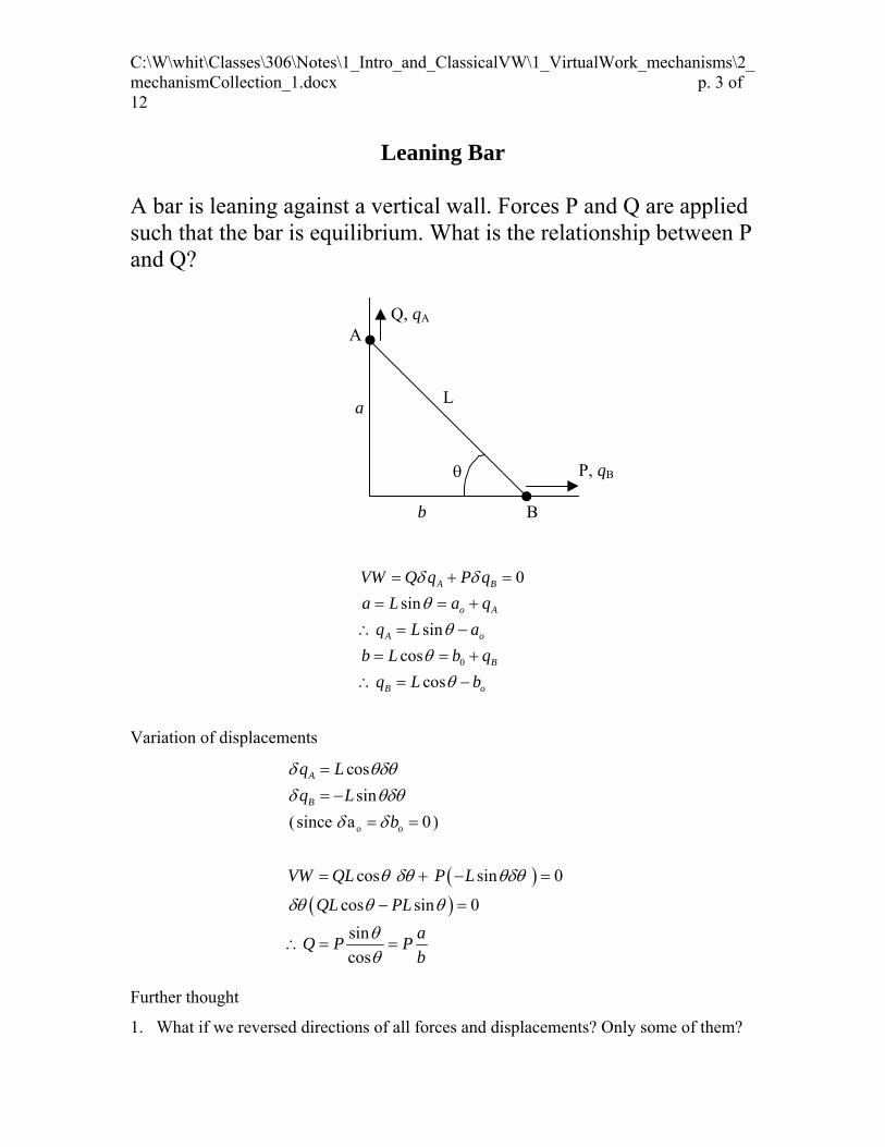
Leaning Bar
A bar is leaning against a vertical wall. Forces P and Q are applied such that the bar is equilibrium. What is the relationship between P and Q?
Q, qA
A
aL
b B
P, qB
0
0
sin
sin
cos
cos
A B
o A
A o
B
B o
VW Q q P q
a L a q
q L a
b L b q
q L b
Variation of displacements
o
cos
sin
(since a 0)
cos sin 0
cos sin 0
sin
cos
A
B
o
q L
q L
b
VW QL P L
QL PL
aQ P P
b
Further thought
1. What if we reversed directions of all forces and displacements? Only some of them?
1/3/2012 p. 37 of 112

C:\W\whit\Classes\306\Notes\1_Intro_and_ClassicalVW\1_VirtualWork_mechanisms\2_mechanismCollection_1.docx p. 4 of 12 2.
Alternative derivations of relationship between qA and qB .
1.
2 2 2
2 2 0
o A A
o B B
A B
a a q a q
b b q b q
a b L
a a b b
ba b
ab
q qa
2.
2 2 2
2 2 2 2 2
2 2
2 2 2
( ) ( )
2 ( ) 2 ( )
( ) ( ) . . .
2 2 0
.
a a b b L
a a a a b b b b L
a and b H O T
and a b L
a a b b
etc
1/3/2012 p. 38 of 112
C:\W\whit\Classes\306\Notes\1_Intro_and_ClassicalVW\1_VirtualWork_mechanisms\2_mechanismCollection_1.docx p. 5 of 12
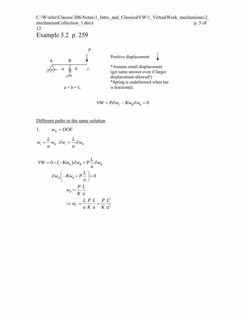
Example 5.2 p. 259
A B
a b c
a + b = L
P
*Assume small displacement (get same answer even if larger displacement allowed!) *Spring is undeformed when bar is horizontal.
Positive displacement
0C B BVW P w Kw w
Different paths to the same solution
1. DOFwB
2
2
0
0
c B c B
B B B
B B
B
C
L Lw w w w
a a
LVW Kw w P w
aL
w Kw Pa
P Lw
K a
L P L P Lw
a K a K a
1/3/2012 p. 39 of 112
C:\W\whit\Classes\306\Notes\1_Intro_and_ClassicalVW\1_VirtualWork_mechanisms\2_mechanismCollection_1.docx p. 6 of 12 2. DOFwC
2
2
2
0
0C
B C B C
C C C
Cw
C
a aw w w w
L L
a aVW K w w P w
L L
aw K P
L
P Lw
K a
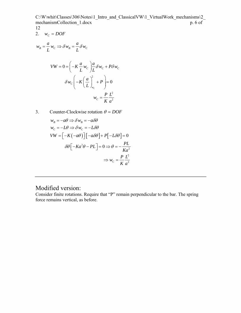
3. Counter-Clockwise rotation DOF
2
2
2
2
0
0
B B
C C
C
w a w a
w L w L
VW K a a P L
PLKa PL
Ka
P Lw
K a
Modified version: Consider finite rotations. Require that “P” remain perpendicular to the bar. The spring force remains vertical, as before.
1/3/2012 p. 40 of 112

C:\W\whit\Classes\306\Notes\1_Intro_and_ClassicalVW\1_VirtualWork_mechanisms\2_mechanismCollection_1.docx p. 7 of 12
Moments & Rotations
P, v
L2L1
M
What is M?
h
PLM
PLM
PLM
Lv
vL
vhLh
vPMW
cos
0cos
0cos
cos
0cos
sin
0
1
1
1
1
1
01
Note: Solution is independent of 2L
Modification: – add torsional spring to right side Assume spring is undeformed when 20 deg Additional term =
where = -20
K
1/3/2012 p. 41 of 112
C:\W\whit\Classes\306\Notes\1_Intro_and_ClassicalVW\1_VirtualWork_mechanisms\2_mechanismCollection_1.docx p. 8 of 12
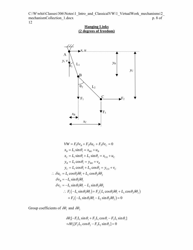
Hanging Links (2 degrees of freedom)
y, v
x, uA
L1
L2
B
C F2F1
F3
1
2
yB
yC
xB
xC
1 2 3
1 1
1 1 2 2
1 1
1 1 2 2
1 1 1 2 2 2
1 1 1
1 1 1 2 2 2
1 1 1 1 2 1 1 1
0
sin
sin sin
cos
cos cos
cos cos
sin
sin sin
sin cos
B C C
B BO B
C CO C
B BO B
C CO C
C
B
C
VW F v F u F v
x L x u
x L L x u
y L y v
y L L y v
u L L
v L
v L L
F L F L
2 2 2
3 1 1 1 2 2 2
cos
sin sin 0
L
F L L
Group coefficients of 1 and 2
1 1 1 1 2 1 1 3 1 1
2 2 2 2 3 2 2
[ sin cos sin ]
[ cos sin ] 0
F L F L F L
F L F L
1/3/2012 p. 42 of 112
C:\W\whit\Classes\306\Notes\1_Intro_and_ClassicalVW\1_VirtualWork_mechanisms\2_mechanismCollection_1.docx p. 9 of 12
Since 1 and 2 are independent and 0, we obtain two equations.
a) 1 1 1 2 1 1 3 1 1sin cos sin 0F L F L F L
b) 2 2 2 3 2 2cos sin 0F L F L
We are lucky….equations are uncoupled
a) 1 1 1 3 2 1 1sin ( ) cos 0L F F F L
1 1 3 2 1
1 2 21
1 1 3 1 3
1 21
1 3
sin ( ) cos
sintan
cos
tan
F F F
F F
F F F F
F
F F
b) 2 2 2 3 2 2cos sin 0F L F L
3 2 2 2
22
3
1 22
3
sin cos
tan
tan ( )
F F
F
F
F
F
Comments
Could have been solved with statics
Solution satisfies “two-force” character of links!
1/3/2012 p. 43 of 112
C:\W\whit\Classes\306\Notes\1_Intro_and_ClassicalVW\1_VirtualWork_mechanisms\2_mechanismCollection_1.docx p. 10 of 12
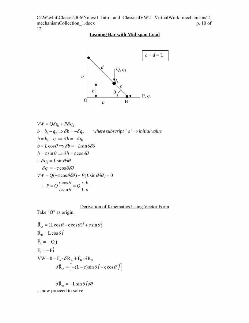
Leaning Bar with Mid-span Load
1 2
0 2 2
0 1 1
2
1
" "
cos sin
sin cos
sin
cos
( cos ) ( sin ) 0
cos
sin
VW Q q P q
b b q b q where subscript o initial value
h h q h q
b L b L
h c h c
q L
q c
VW Q c P L
c c bP Q Q
L L a
Derivation of Kinematics Using Vector Form Take "O" as origin.
A
B
A
B
A A B B
A
B
ˆˆR (Lcos ccos ) csin j
ˆR Lcos
ˆF Q j
ˆF Pi
VW = 0 = F R F R
ˆ ˆR (L c)sin ccos
ˆR Lsin
i
i
i j
i
…now proceed to solve
P, q2
c
b
a
d Q, q1
c + d = L
h
A
BO
1/3/2012 p. 44 of 112
C:\W\whit\Classes\306\Notes\1_Intro_and_ClassicalVW\1_VirtualWork_mechanisms\2_mechanismCollection_1.docx p. 11 of 12
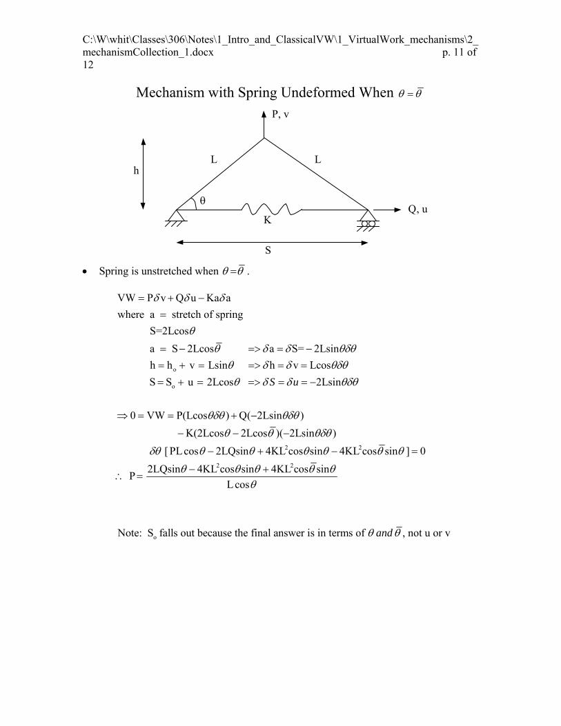
Mechanism with Spring Undeformed When
L L h
S
P, v
K Q, u
Spring is unstretched when .
o
o
VW P v Q u Ka a
where a stretch of spring
S=2Lcos
a S 2Lcos a S= 2Lsin
h h v Lsin h v Lcos
S S u 2Lcos 2Lsin
0 VW P(Lcos ) Q( 2Lsin )
K(2Lcos 2Lcos )( 2Lsin )
[ PLco
S u
2 2
2 2
o
s 2LQsin 4KL cos sin 4KL cos sin ] 0
2LQsin 4KL cos sin 4KL cos sinP
Lcos
Note: S falls out because the final answer is in terms of , not u or vand
1/3/2012 p. 45 of 112

C:\W\whit\Classes\306\Notes\1_Intro_and_ClassicalVW\1_VirtualWork_mechanisms\2_mechanismCollection_1.docx p. 12 of 12
Two-degree of Freedom Problem Assume springs stay vertical
1/3/2012 p. 46 of 112

2a_leaningBar_and_Spring_Stability.mw p. 1 of 6
> > (1)(1)
leaningBar_and_Spring_Stability.mw
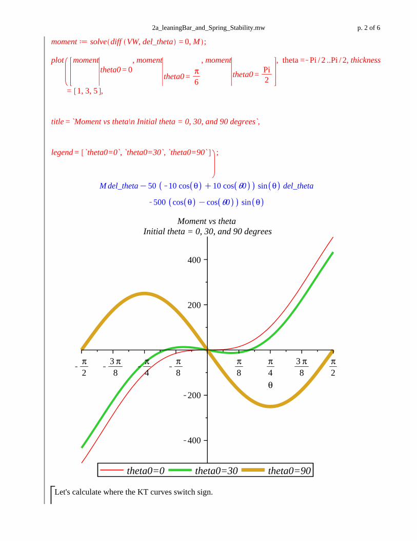
Looking at moment vs theta we can extract the tangential stiffness, which reveals whether the equilibrium state is stable.
More directly, we can calculate the tangential stiffness. Negative tangential stiffness implies instability. If there is more than one degree of freedom, the sign of the determinant of the "stiffness matrix" will indicate stability. We will study this much more later in the semeter.
restart:currentdir();"C:\W\whit\Classes\306\Notes\1_Intro_and_ClassicalVW\1_VirtualWork_mechanisms"
Behavior for three configurations In each case, the spring is compressed or has zero deformation when theta = 0.
These results show that the stability of the configuration depends on both the theta corresponding to an unstretched spring and also the equilibrium state.
Value of angle theta when spring is unstretched
Behavior
0 always unstable
30 unstable for theta less than 17 deg.
90 unstable for theta less than 45 deg.
I should point out that if the spring is in tension even when theta =0, then the story changes. We will consider that case later.L d 10 :K d 5 : VW d M * del_thetaKK * KL* cos theta C L* cos theta0 * L * sin theta * del_theta;
1/3/2012 p. 47 of 112
2a_leaningBar_and_Spring_Stability.mw p. 2 of 6
moment d solve diff VW, del_theta = 0, M ;
plot momenttheta0 = 0
, moment
theta0 =π6
, moment
theta0 =Pi2
, theta =KPi / 2 ..Pi / 2, thickness
= 1, 3, 5 ,
title = `Moment vs theta\n Initial theta = 0, 30, and 90 degrees ,̀
legend = `theta0=0`, `theta0=30`, `theta0=90` ;
M del_thetaK50 K10 cos θ C10 cos θ0 sin θ del_theta
K500 cos θ Kcos θ0 sin θ
theta0=0 theta0=30 theta0=90
θ
Kπ2
K3 π8
Kπ4
Kπ8
π8
π4
3 π8
π2
K400
K200
200
400
Moment vs theta Initial theta = 0, 30, and 90 degrees
Let's calculate where the KT curves switch sign.
1/3/2012 p. 48 of 112

2a_leaningBar_and_Spring_Stability.mw p. 3 of 6
> >
> >
(1.1)(1.1)
KT := -diff(VW,del_theta, theta);crossover_0 := evalf( fsolve(eval(KT, theta0= 0) =0, theta= 0..Pi/2) * 180/Pi );crossover_30 := evalf( fsolve(eval(KT, theta0= Pi/6) =0, theta= 0..Pi/2) * 180/Pi );crossover_90 := evalf( fsolve(eval(KT, theta0= Pi/2) =0, theta= 0..Pi/2) * 180/Pi );
KT := 500 sin θ2C50 K10 cos θ C10 cos θ0 cos θ
crossover_0 := 0.
crossover_30 := 17.05643285
crossover_90 := 44.99999998
plot( [subs(theta0=0,KT), subs(theta0=Pi/6,KT), subs(theta0=Pi/2,KT)],theta= -Pi/2..Pi/2,thickness=[1,3,5], title=`Tangential stiffness vs theta`,legend=[`theta0=0`, `theta0=30`, `theta0=90`]);
1/3/2012 p. 49 of 112

2a_leaningBar_and_Spring_Stability.mw p. 4 of 6
theta0=0 theta0=30 theta0=90
θ
Kπ2
K3 π8
Kπ4
Kπ8
π8
π4
3 π8
π2
K400
K200
200
400
Tangential stiffness vs theta
This is a bit more general. When the spring is horizontal, the stretch of the spring = c*L. Depending on the value chosen for c, very different behaviors are observed. Let's assume that the unstrectched length of the spring is such that when theta =0, the spring is under tension is c>0. The stretch when theta =0 is c * L.W=Lcos(theta) + S => S = W-Lcos(theta) Stretch of spring = S - S_unstretched = (W-Lcos(theta) ) - (W- L - c*L) Therefore, the stretch = -Lcos(theta) + L + c*L.Note that the tangential stiffness (i.e. the slope for this 1-dof problem) is always positive if the spring is in tension when it is horizontal.L d 10 :K d 5 :
VW d M * del_theta KK * KL* cos theta C L C c$L * L * sin theta * del_theta;moment d solve diff VW, del_theta = 0, M ;plot eval moment, c =K.2 , eval moment, c =K.4 , eval moment, c = .2 , eval moment, c = .4 ,
theta =KPi / 2 ..Pi / 2, thickness = 3, title = `Moment vs theta\n ,̀ thickness = 1, 2, 3 , color = red, green, blue , legend = `c= -.2`, `c= -.4 ,̀ `c=.2 ,̀ `c=.4` ;
1/3/2012 p. 50 of 112

2a_leaningBar_and_Spring_Stability.mw p. 5 of 6
> >
M del_thetaK50 K10 cos θ C10C10 c sin θ del_theta
K500 cos θ K1Kc sin θ
c= -.2 c= -.4 c=.2 c=.4
θ
Kπ2
K3 π8
Kπ4
π8
π4
3 π8
π2
K600
K400
K200
200
400
600
Moment vs theta
KT := -diff(VW,del_theta, theta);plot( [subs(c= -.4,KT), subs(c= -.2,KT), subs(c= .2,KT), subs(c= .4,KT)], theta= -Pi/2..Pi/2,thickness=[1,2,3,4], title=`Tangential stiffness vs theta`, legend=[`c= -.2`, `c= -.4`, `c=.2`, `c=.4`], color = [red, green, blue]);
KT := 500 sin θ2C50 K10 cos θ C10C10 c cos θ
1/3/2012 p. 51 of 112

2a_leaningBar_and_Spring_Stability.mw p. 6 of 6
> >
c= -.2 c= -.4 c=.2 c=.4
θ
Kπ2
K3 π8
Kπ4
π8
π4
3 π8
π2
K200
K100
100
200
300
400
500
600
Tangential stiffness vs theta
1/3/2012 p. 52 of 112
Dec 29, 2011 3a_landingGear.mw 1 of 4
> >
(1)(1)
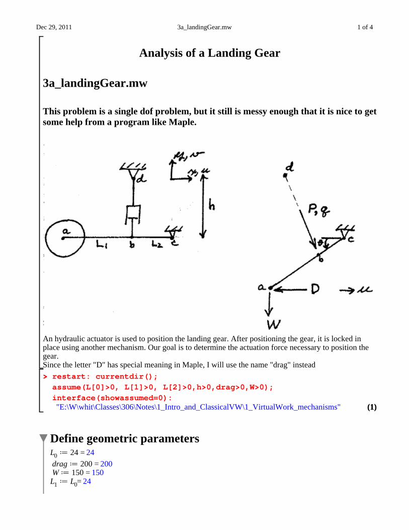
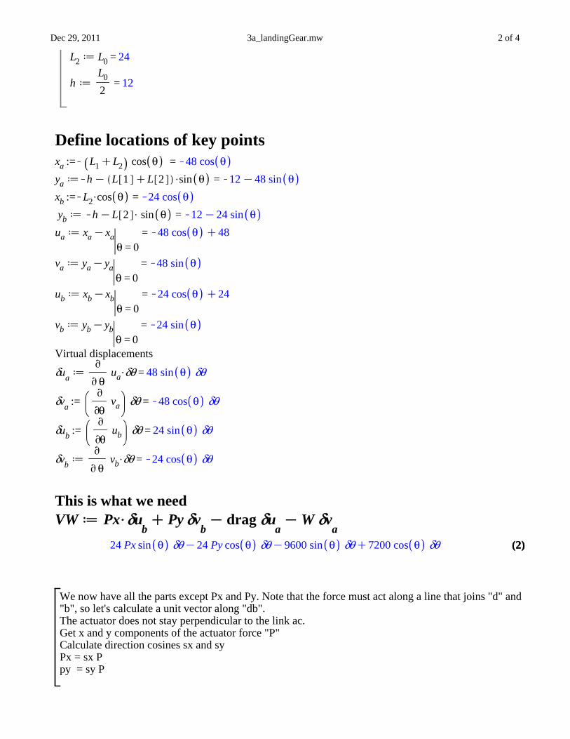
Analysis of a Landing Gear
3a_landingGear.mw
This problem is a single dof problem, but it still is messy enough that it is nice to getsome help from a program like Maple.
An hydraulic actuator is used to position the landing gear. After positioning the gear, it is locked in place using another mechanism. Our goal is to determine the actuation force necessary to position the gear.Since the letter "D" has special meaning in Maple, I will use the name "drag" instead
restart: currentdir();assume(L[0]>0, L[1]>0, L[2]>0,h>0,drag>0,W>0);interface(showassumed=0):"E:\W\whit\Classes\306\Notes\1_Intro_and_ClassicalVW\1_VirtualWork_mechanisms"
Define geometric parametersL0 d 24 = 24
drag d 200 = 200 Wd 150 = 150L1 d L0= 24
1/3/2012 p. 53 of 112
Dec 29, 2011 3a_landingGear.mw 2 of 4
(2)(2)
L2 d L0 = 24
h dL0
2 = 12
Define locations of key pointsxa :=K L1CL2 cos θ = K48 cos θya dKhK L 1 CL 2 $sin θ = K12K48 sin θxb :=KL2$cos θ = K24 cos θ
yb d KhKL 2 $ sin θ = K12K24 sin θua d xaKxa
θ = 0 = K48 cos θ C48
va d yaKyaθ = 0
= K48 sin θ
ub d xbKxbθ = 0
= K24 cos θ C24
vb d ybKybθ = 0
= K24 sin θ
Virtual displacements
δua dv
v θ ua$δθ = 48 sin θ δθ
δva
:=v
vθ va δθ = K48 cos θ δθ
δub :=v
vθ ub δθ = 24 sin θ δθ
δvb dv
v θ vb$δθ = K24 cos θ δθ
This is what we needVWd Px$δu
bC Py δv
bK drag δu
aKW δv
a
24 Px sin θ δθK24 Py cos θ δθK9600 sin θ δθC7200 cos θ δθ
We now have all the parts except Px and Py. Note that the force must act along a line that joins "d" and "b", so let's calculate a unit vector along "db".The actuator does not stay perpendicular to the link ac.Get x and y components of the actuator force "P"Calculate direction cosines sx and syPx = sx Ppy = sy P
1/3/2012 p. 54 of 112

Dec 29, 2011 3a_landingGear.mw 3 of 4
(3)(3)
Δx d L2KL2 cos θ = K24 cos θ C24
Δy dKhKL2 sin θ = K12K24 sin θ
len d Δx2CΔy
2 = K24 cos θ C24
2C K12K24 sin θ
2 assuming real
12 9K8 cos θ C4 sin θ
sx :=Δxlen
= K24 cos θ C24
K24 cos θ C242C K12K24 sin θ
2
assuming real
K2 cos θ K1
9K8 cos θ C4 sin θ
sydΔylen
= K12K24 sin θ
K24 cos θ C242C K12K24 sin θ
2
assuming real
K1C2 sin θ
9K8 cos θ C4 sin θ
Px d sx P = K24 cos θ C24 P
K24 cos θ C242C K12K24 sin θ
2
assuming real
K2 P cos θ K1
9K8 cos θ C4 sin θ
Py d sy P = K12K24 sin θ P
K24 cos θ C242C K12K24 sin θ
2
assuming real
KP 1C2 sin θ
9K8 cos θ C4 sin θ
Now we can calculate the virtual work and solve for P in terms of theta
VW d Px$δubCPy δvbKdrag δuaKW δva
24 K24 cos θ C24 P sin θ δθ
K24 cos θ C242C K12K24 sin θ
2
K24 K12K24 sin θ P cos θ δθ
K24 cos θ C242C K12K24 sin θ
2K9600 sin θ δθC7200 cos θ δθ
Set the Virtual Work to zero and solve for the actuatorForce d solve VW = 0, P =
K100 4 cos θ
2K8 cos θ C5C4 sin θ C4 sin θ
2 K4 sin θ C3 cos θ
2 sin θ Ccos θ
1/3/2012 p. 55 of 112

Dec 29, 2011 3a_landingGear.mw 4 of 4
(4)(4)
> >
Now let's plot the variation of the actuator force with position. Does this plot make physical sense? Explain. plot actuatorForce, θ = 0 ..π / 2, thickness = 3, title = `Actuator force vs theta`
θ0.5 1 1.5
K200
0
200
400
600
Actuator force vs theta
Let's look at the actuator force for a couple of values of theta.[eval(actuatorForce,theta=0),eval(actuatorForce,theta=Pi/2.),evalf(eval(actuatorForce,theta=Pi/2.))];
K300, 200 13 , 721.1102550
1/3/2012 p. 56 of 112

C:\W\whit\Classes\306\Notes\1_Intro_and_ClassicalVW\1_VirtualWork_mechanisms\4_linearApproximation.docx 01/03/12 Page 1 of 2
Introduction to Linear Deformable Systems Motivation: Unless we make assumptions about small deformations and rotations, even many “simple” problems are quite complicated to analyze. What is a linear system? What is the behavior of a linear system in terms of…
force vs. displacement superposition spring constants material response geometric linearity (small translations and rotations) => final configuration is
very similar to original! A simple example is studied in the file singleSpring_Nonlinear&Linear.mw. Note that the linear approximation is much simpler. It is also only valid for small changes in the structure. The worksheet singleSpring_Nonlinear&Linear.mw obtained a linearized solution, but it did not go on to explain a simple way to exploit the assumption of linearity. The following will show that describing the deformation of a two-force member that undergoes very small motion is very simple. Link to pdf of the file: singleSpring_Nonlinear&Linear.pdf (might not be the latest)
Two-Force Members: Linear Approximation
Displacements at each end = u, v Definitions relative x-displacement = right leftu u u
relative y-displacement = right leftv v v
right leftx x x right lefty y y
First, get an expression for the length of the member after deformation.
1/ 2 1/ 22 2 2 2
0L x y L x u y v
If you multiply out the expression for L, you will find some of the terms combine to equal Lo. Hence, the expression for L becomes
1/ 22 2 20 2 2L L xu y v u v
Now the challenge is to determine how much the length changes when the displacements are very small. Let's get an approximation for L by using a Taylor series expansion
1/3/2012 p. 57 of 112

C:\W\whit\Classes\306\Notes\1_Intro_and_ClassicalVW\1_VirtualWork_mechanisms\4_linearApproximation.docx 01/03/12 Page 2 of 2
1/2 1/22 20 0 0
00 0
0
0, 00, 0
( , ) (0,0)
1 12 2
2 2
( , ) cos sin
where the angle is determined from the initial (undeformed) state
||u vu v
L LL u v L u v
u v
L x L u y L v
x yL u v
L L
L u v L u v
That is, the change in length is simply cos sin
This could also be expressed as the dot product
(displacement vector) (unit vector parallel to truss member)
u v
In Aero 306 we will almost always assume linearity when analyzing trusses. This is because the problems become very difficult otherwise. Also, the linear approximation is generally a good engineering approximation! Optional thoughts & exercises One could also determine the formula for the change in length by calculating the
differential dL. Compare expression obtained above for the Taylor series expansion with the differential.
Calculate first and second order Taylor series expansions for sine and cosine. There are a couple of Maple worksheets that examine a little more complicated
configurations. 4a_3Spring_nonlinear.mw. and 4b_3Spring.mw.
1/3/2012 p. 58 of 112

Dec 29, 2011 5_singleSpring_Nonlinear&Linear.mw 1 of 5
(1.1)(1.1)
5_singleSpring_Nonlinear&Linear.mw
This structure is related to a single member of a 3-D space truss like you would find on the space station.We will use this structure to illustrate what it means to obtain linearized equations. We will first analyze the configuration without geometric approximation. We will obtain a nonlinear equilibrium equation, which is not easy to solve even though the problem seems quite simple. Then we will assume that the motion of the spring is quite small. This will allow us to obtain a linear approximation of the behavior ofthe spring. The governing eqution then becomes very simple.
For the small load (F=1), the predicted displacement from the nonlinear and linear analyses is almost thesame. When F=100, the displacement "u" is much larger and the agreement is very bad. This is as expected.
Large load: F = 100Very small load: F = 1
First we will solve the nonlinear version two ways. Then we will solve the linearized version.
Nonlinear Analysis
Solution using "u" as the dofrestart : currentdir ;
"C:\W\whit\Classes\306\Notes\1_Intro_and_ClassicalVW\1_VirtualWork_mechanisms"params d F = 1, K = 30, a = 10 :
θ0 d Pi6
:
1/3/2012 p. 59 of 112

Dec 29, 2011 5_singleSpring_Nonlinear&Linear.mw 2 of 5
(1.2)(1.2)
(1.3)(1.3)
L0 d a
cos θ0
:
H0 d L0 $ sin θ0 :
H d H0 C u : L d sqrt a2CH2 :
Stretch of spring: springStretch d LKL0; = a2C13
a 3 Cu2
K23
a 3
δspringStretch d diff springStretch, u $ δu; = 12
23
a 3 C2 u δu
a2C13
a 3 Cu2
virtualWork d F$δuKK$springStretch$δspringStretch =
F δuK 12
K a2C
13
a 3 Cu2
K23
a 3 23
a 3 C2 u δu
a2C13
a 3 Cu2
Set coefficient of variation =0.
solvev
v δ̀u` virtualWork = 0, u
K 3 F RootOf 3 _Z4 K2K4 _Z3 K2 3 aC K3 F2CK2 a2 _Z2C4 K2 _Z a3 3
K4 K2 a4 KK RootOf 3 _Z4 K2K4 _Z3 K2 3 aC K3 F2CK2 a2 _Z2
C4 K2 _Z a3 3 K4 K2 a4 a 3 C2 K a2 2 a 3 K3 RootOf 3 _Z4 K2
K4 _Z3 K2 3 aC K3 F2CK2 a2 _Z2C4 K2 _Z a3 3 K4 K2 a4 KAs you can see, this is a mess. Let's just get the solution for a particular case. In fact, even whenI substitute in numerical values for F, K, and a, Maple does not give a solution with "solve". I have to use fsolve which searches for a numerical (rather than a symbolic) solution.VW d subs params, virtualWork : print `The virtual work = `, VW ;
u d fsolvev
v δ̀u` VW = 0, u :
print `The displacement u = `, u ; angle d solve H0 Cu = L$sin θ , theta :
angle d evalfsubs params, angle $ 180.
Pi;
The virtual work = , δu
K15 100C
103
3 Cu2
K203
3 203
3 C2 u δu
100C103
3 Cu2
The displacement u = , 0.1300444212
30.55567813
1/3/2012 p. 60 of 112

Dec 29, 2011 5_singleSpring_Nonlinear&Linear.mw 3 of 5
(2.1)(2.1)
Solution using as the dof
θ0 d Pi6
= 16
π
L d a
cos theta =
a
cos θ
L0 d a
cos θ0
= 23
a 3
H d L $ sin θ = a sin θcos θ
H0 d L0 $ sin θ0
= 13
a 3
u d 'u ':
u d solve H = H0 C u, u = K13
a 3 cos θ K3 sin θ
cos θ
δ̀u` :=v
vθ u δ̀θ ;̀
δ̀u` := simplify δ̀u` =
K13
a K 3 sin θ K3 cos θ
cos θK
13
a 3 cos θ K3 sin θ sin θ
cos θ2
δθ
δθ a
cos θ2
Stretch of spring: springStretch d LKL0; = a
cos θK
23
a 3
δ̀springStretch` :=v
vθ springStretch δ̀θ ̀=
a sin θ δθ
cos θ2
virtualWork d F$δuKK$springStretch$δspringStretch =
F δθ a
cos θ2K
K a
cos θK
23
a 3 a sin θ δθ
cos θ2
#params:= F = 100, K = 30, a = 10 :VW d subs params, virtualWork : print `The virtual work = `, VW ;
θ d fsolvev
vδθ VW = 0, θ = 0 ..
Pi2
:
print The angle θ = , evalfθ $ 180
Pi;
The virtual work = ,10 δθ
cos θ2 K
300 10
cos θK
203
3 sin θ δθ
cos θ2
1/3/2012 p. 61 of 112

Dec 29, 2011 5_singleSpring_Nonlinear&Linear.mw 4 of 5
(3.1.1)(3.1.1)
(2.3)(2.3)
(2.2)(2.2)The angle θ = , 30.55567814evalf subs params, HKH0
0.130044418
Linear Analysis
Linear approximationFor simplicity, we will only consider one case: Assume the spring is unstretched initially, which means that the angle theta is initially 30 degrees. We will assume that the force is small enough that the displacement "u" is very small. We will derive a linearized equilibrium equation that will predict the relationship between F and u quite well as long as "u" is very small.
Linear solution using "u" as the dofrestart : params d F = 1, K = 30, a = 10 :
θ0 d Pi6
:
L0 d a
cos θ0
;
H0 d L0 $ sin θ0 ;
H d H0 C u;
L d sqrt a2CH2 : print `L = ,̀ L ;
23
a 3
13
a 3
13
a 3 Cu
L = , a2C13
a 3 Cu2
We started off the same way as before, but we have hit a snag. The expression for "L" is a nonlinear function of "u". This means that the deformation is a nonlinear function of "u". This means that we are going to end up with a nonlinear equilibrium equation unless we do something. We need to obtain a linear approximation for how L depends on u. The most convenient techniqueis using the Taylor Series Expansion. A first order Taylor series expansion about u=0 is
L := Lu = 0
Cv
vu L
u = 0
u = 13
4 3 a2 C14
4 a u
a2
Note that in this approximation, the length L varies linearly with u.
Stretch of spring: springStretch d LKL0; = 13
4 3 a2 C14
4 a u
a2K
23
a 3
This can be simplified some: interface showassumed = 0 : assume a O 0 :
1/3/2012 p. 62 of 112

Dec 29, 2011 5_singleSpring_Nonlinear&Linear.mw 5 of 5
springStretch d simplify springStretch ; = 12
u
δ̀springStretch` :=v
vu springStretch δ̀u ̀=
12
δu
virtualWork d F$δuKK$springStretch$δspringStretch = F δuK 14
K u δu
Set coefficient of variations =0.u d'u ':
u d solvev
v δ̀u` virtualWork = 0, u =
4 FK
As you can see, this is much simpler than we obtained with the nonlinear description. Let's get thesolution for the same loading, etc. that we considered earlier.ans d subs params, u : print `u = `, evalf ans ; = u = , 0.1333333333Summary of results
u for F= 1 u for F=100
Nonlinear .130 6.516
Linear .133 13.3
Note that the linear approximation is awful for F= 100 but very good for F= 1.
What if the spring is undeformed when theta=30 degrees, but the initial configuration is theta = 60 degrees? Strategy: obtain an exact expression for the length and deformation when theta = 60 degrees. Then take a Taylor series expansion about the state theta = 60 degrees (this can also be expressed in terms of u). We will end up with a linear equilibrium equation for this new starting condition. Because of lack of time, we will not cover this case in aero 306.
1/3/2012 p. 63 of 112
Dec 29, 2011 6a_selfStudy_springs_3_linear.mw 1 of 2
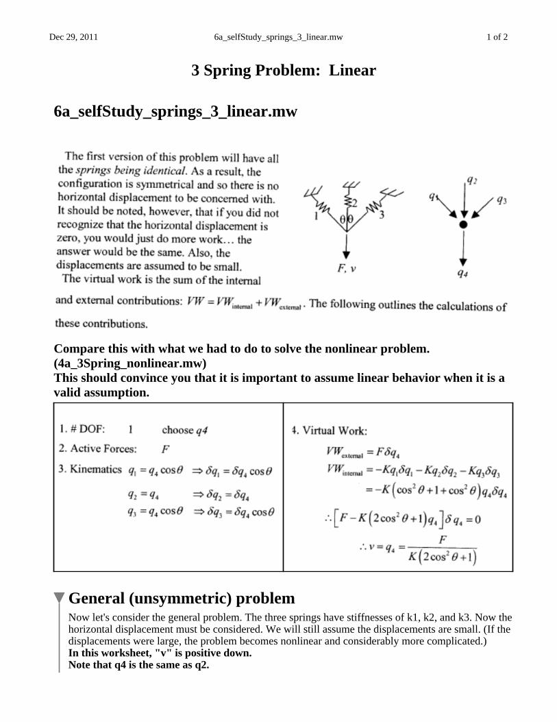
3 Spring Problem: Linear
6a_selfStudy_springs_3_linear.mw
Compare this with what we had to do to solve the nonlinear problem. (4a_3Spring_nonlinear.mw)This should convince you that it is important to assume linear behavior when it is a valid assumption.
General (unsymmetric) problemNow let's consider the general problem. The three springs have stiffnesses of k1, k2, and k3. Now thehorizontal displacement must be considered. We will still assume the displacements are small. (If the displacements were large, the problem becomes nonlinear and considerably more complicated.)In this worksheet, "v" is positive down.Note that q4 is the same as q2.
1/3/2012 p. 64 of 112
Dec 29, 2011 6a_selfStudy_springs_3_linear.mw 2 of 2
(1.1)(1.1)
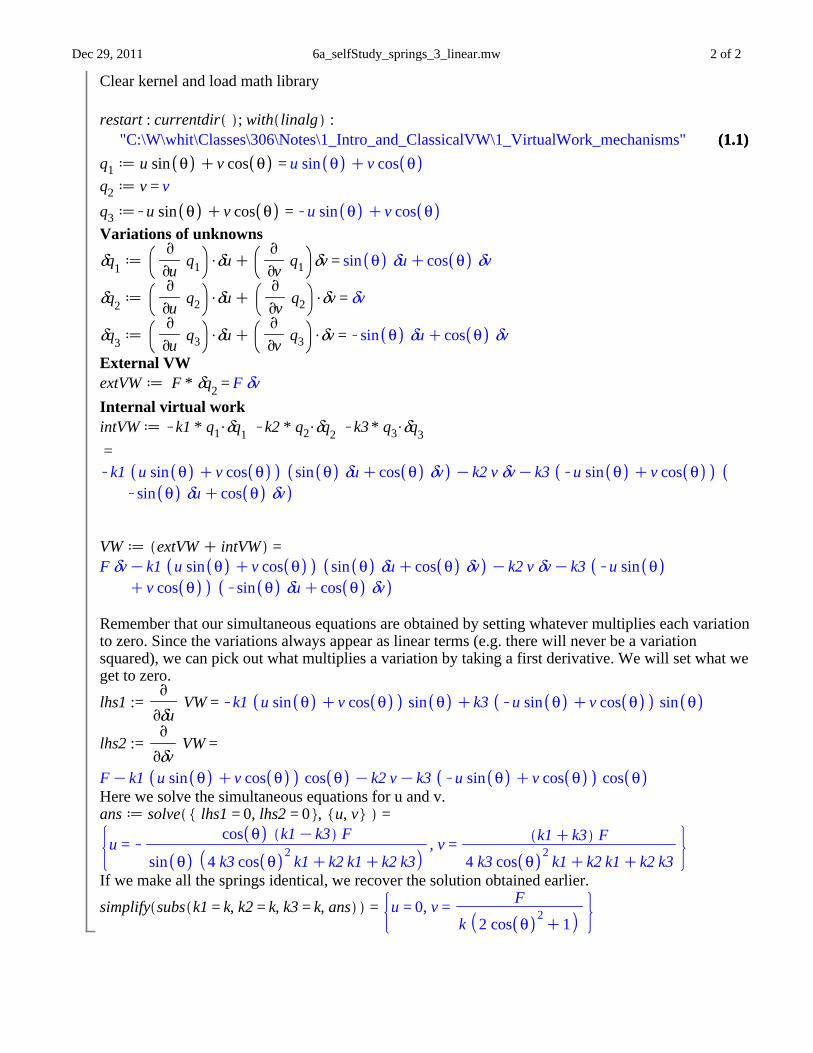
Clear kernel and load math library
restart : currentdir ; with linalg :"C:\W\whit\Classes\306\Notes\1_Intro_and_ClassicalVW\1_VirtualWork_mechanisms"
q1 d u sin θ Cv cos θ = u sin θ Cv cos θq2 d v = v
q3 dKu sin θ Cv cos θ = Ku sin θ Cv cos θVariations of unknowns
δq1d
v
vu q1 $δuC
v
vv q1 δv = sin θ δuCcos θ δv
δq2 dv
vu q2 $δuC
v
vv q2 $δv = δv
δq3 d v
vu q3 $δuC
v
vv q3 $δv = Ksin θ δuCcos θ δv
External VWextVW d F * δq2 = F δvInternal virtual workintVW d Kk1 * q1$δq1 Kk2 * q2$δq2 Kk3 * q3$δq3
= Kk1 u sin θ Cv cos θ sin θ δuCcos θ δv Kk2 v δvKk3 Ku sin θ Cv cos θ
Ksin θ δuCcos θ δv
VW d extVW C intVW = F δvKk1 u sin θ Cv cos θ sin θ δuCcos θ δv Kk2 v δvKk3 Ku sin θ
Cv cos θ Ksin θ δuCcos θ δv
Remember that our simultaneous equations are obtained by setting whatever multiplies each variationto zero. Since the variations always appear as linear terms (e.g. there will never be a variation squared), we can pick out what multiplies a variation by taking a first derivative. We will set what weget to zero.
lhs1 :=v
vδu VW = Kk1 u sin θ Cv cos θ sin θ Ck3 Ku sin θ Cv cos θ sin θ
lhs2 :=v
vδv VW =
FKk1 u sin θ Cv cos θ cos θ Kk2 vKk3 Ku sin θ Cv cos θ cos θHere we solve the simultaneous equations for u and v.ans d solve lhs1 = 0, lhs2 = 0 , u, v =
u =Kcos θ k1Kk3 F
sin θ 4 k3 cos θ2 k1Ck2 k1Ck2 k3
, v =k1Ck3 F
4 k3 cos θ2 k1Ck2 k1Ck2 k3
If we make all the springs identical, we recover the solution obtained earlier.
simplify subs k1 = k, k2 = k, k3 = k, ans = u = 0, v =F
k 2 cos θ2C1
1/3/2012 p. 65 of 112
Dec 29, 2011 6b_selfStudy_springs_3_nonlinear.mw 1 of 4
(1)(1)
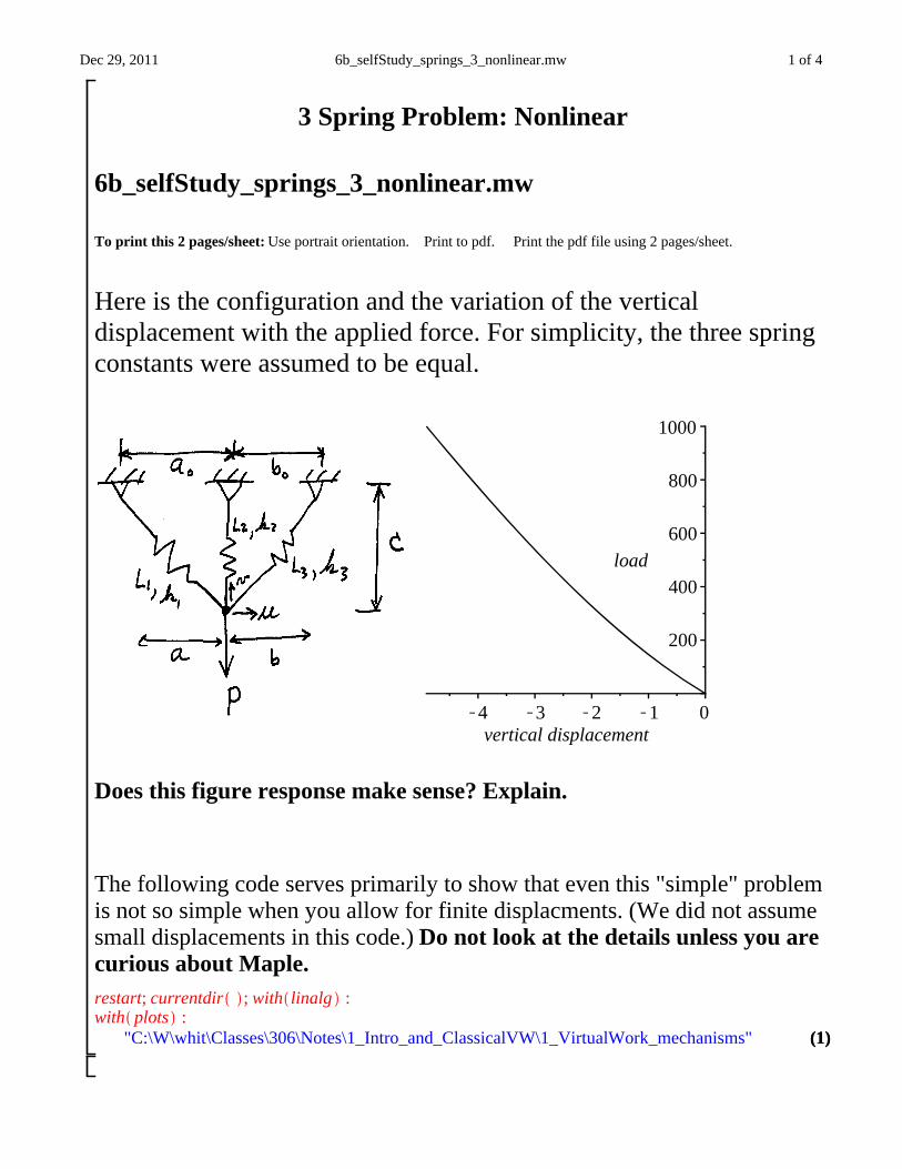
3 Spring Problem: Nonlinear
6b_selfStudy_springs_3_nonlinear.mw
To print this 2 pages/sheet: Use portrait orientation. Print to pdf. Print the pdf file using 2 pages/sheet.
Here is the configuration and the variation of the vertical displacement with the applied force. For simplicity, the three spring constants were assumed to be equal.
vertical displacementK4 K3 K2 K1 0
load
200
400
600
800
1000
Does this figure response make sense? Explain.
The following code serves primarily to show that even this "simple" problem is not so simple when you allow for finite displacments. (We did not assume small displacements in this code.) Do not look at the details unless you are curious about Maple.restart; currentdir ; with linalg :with plots :
"C:\W\whit\Classes\306\Notes\1_Intro_and_ClassicalVW\1_VirtualWork_mechanisms"
1/3/2012 p. 66 of 112

Dec 29, 2011 6b_selfStudy_springs_3_nonlinear.mw 2 of 4
> >
(3)(3)> >
> >
(4)(4)
(2)(2)
Assign values of parameters. For simplicity (the problem is still not simple!), we will set the spring constants equal.a0 d 5 : b0 d 5 : c0 d 2 : k d 100 : k1 d k : k2 d k : k3 := k :Define dimensions in terms of displacements. L1=current length L01= initial length, etc.
a d a0Cu; b := b0Ku; c d c0Kv;
L1 := a2Cc2 ; L2 d c; L3 d b2Cc2 ;
L01 d subs u = 0, v = 0, L1 ; L02 d subs u = 0, v = 0, L2 ; L03 d subs u = 0, v = 0, L3 ;
a := 5Cu
b := 5Ku
c := 2Kv
L1 := 29C10 uCu2K4 vCv2
L2 := 2Kv
L3 := 29K10 uCu2K4 vCv2
L01 := 29
L02 := 2
L03 := 29
Maple note: We can format the formulas and the output differently if we put the lines in a document block. The ":=" is assigning a value. The "=" in this case is just showing the result of theassignment.
δL1 d v
vu L1 $δuC
v
vv L1 $δv =
12
10C2 u δu
29C10 uCu2K4 vCv2C
12
K4C2 v δv
29C10 uCu2K4 vCv2
δL2 dv
vu L2 $δu C
v
vv L2 $δv = Kδv
δL3 d v
vu L3 $δuC
v
vv L3 $δv =
12
K10C2 u δu
29K10 uCu2K4 vCv2C
12
K4C2 v δv
29K10 uCu2K4 vCv2
External VWextVW dKF$δv
extVW := KF δv
Internal VWintVW :=Kk1 L1KL01 δL1Kk2 L2KL02 δL2Kk3 L3KL03 δL3
intVW := K100 29C10 uCu2K4 vCv2 K 29 12
10C2 u δu
29C10 uCu2K4 vCv2
1/3/2012 p. 67 of 112
Dec 29, 2011 6b_selfStudy_springs_3_nonlinear.mw 3 of 4
> >
(5)(5)
> >
> >
C12
K4C2 v δv
29C10 uCu2K4 vCv2K100 v δvK100 29K10 uCu2K4 vCv2
K 29 12
K10C2 u δu
29K10 uCu2K4 vCv2C
12
K4C2 v δv
29K10 uCu2K4 vCv2
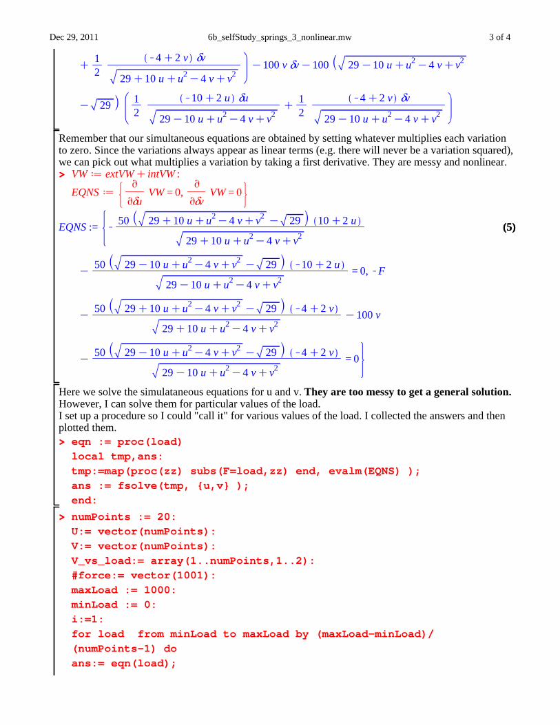
Remember that our simultaneous equations are obtained by setting whatever multiplies each variation to zero. Since the variations always appear as linear terms (e.g. there will never be a variation squared), we can pick out what multiplies a variation by taking a first derivative. They are messy and nonlinear.
VW d extVWCintVW :
EQNS dv
vδu VW = 0,
v
vδv VW = 0
EQNS := K50 29C10 uCu2K4 vCv2 K 29 10C2 u
29C10 uCu2K4 vCv2
K50 29K10 uCu2K4 vCv2 K 29 K10C2 u
29K10 uCu2K4 vCv2= 0, KF
K50 29C10 uCu2K4 vCv2 K 29 K4C2 v
29C10 uCu2K4 vCv2K100 v
K50 29K10 uCu2K4 vCv2 K 29 K4C2 v
29K10 uCu2K4 vCv2= 0
Here we solve the simulataneous equations for u and v. They are too messy to get a general solution. However, I can solve them for particular values of the load. I set up a procedure so I could "call it" for various values of the load. I collected the answers and then plotted them.eqn := proc(load)local tmp,ans:tmp:=map(proc(zz) subs(F=load,zz) end, evalm(EQNS) );ans := fsolve(tmp, {u,v} );end:
numPoints := 20:U:= vector(numPoints):V:= vector(numPoints):V_vs_load:= array(1..numPoints,1..2):#force:= vector(1001):maxLoad := 1000:minLoad := 0:i:=1:for load from minLoad to maxLoad by (maxLoad-minLoad)/(numPoints-1) doans:= eqn(load);
1/3/2012 p. 68 of 112

Dec 29, 2011 6b_selfStudy_springs_3_nonlinear.mw 4 of 4
> >
U[i]:= subs(ans,u):V[i]:= subs(ans,v):#force[i] := load:V_vs_load[i,1] := V[i]:V_vs_load[i,2] := load:# print(U[i], V[i]);i:=i+1:od:
listplot(V_vs_load,labels=[`vertical displacement`,'load']);
vertical displacementK4 K3 K2 K1 0
load
200
400
600
800
1000
1/3/2012 p. 69 of 112
C:\W\whit\Classes\306\Notes\1_Intro_and_ClassicalVW\2_VirtualWork_approxSolution\1_discreteSolutions.doc 1 of 16
Analysis of Uniaxial Bars and Beams Using
Discrete Virtual Work Quick review of uniaxial bars Derive Virtual Work expressions for uniaxial bar Example exact Virtual Work solutions for uniaxial bar Approximate Virtual Work solution for uniaxial bar Example approximate solutions Repeat this for beams
1/3/2012 p. 70 of 112
C:\W\whit\Classes\306\Notes\1_Intro_and_ClassicalVW\2_VirtualWork_approxSolution\1_discreteSolutions.doc 2 of 16
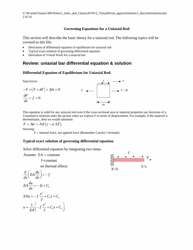
Governing Equations for a Uniaxial Rod
This section will describe the basic theory for a uniaxial rod. The following topics will be covered in this file: Derivation of differential equation of equilibrium for uniaxial rod Typical exact solution of governing differential equation Derivation of Virtual Work for a uniaxial bar
Review: uniaxial bar differential equation & solution
Differential Equation of Equilibrium for Uniaxial Rod Sum forces
0
0
F F dF fdx
dFf
dx
This equation is valid for any uniaxial rod even if the cross sectional area or material properties are functions of x. Constitutive relations enter the picture when we express F in terms of displacement. For example, if the material is thermoelastic, then we would substitute
F A A E T
Warning: F = internal force, not applied force (Remember Cauchy’s formula) Typical exact solution of governing differential equation
1
2
1 2
2
1 2
Solve differential equation by integrating two times
Assume: EA constant
f=constant
no thermal effects
2
1
2
d duEA f
dx dx
duEA fx C
dx
xEAu f C x C
xu f C x C
EA
F F + dF
dx
f u
Pf
X=LX=0
1/3/2012 p. 71 of 112

C:\W\whit\Classes\306\Notes\1_Intro_and_ClassicalVW\2_VirtualWork_approxSolution\1_discreteSolutions.doc 3 of 16
Now impose the boundary conditions (0) 0x L
duu and EA P
dx
to determineC1 and C2
2 2
1
1
2
11) (0) 0 (0 0 ) 0 0
12)
1 This is the exact solution.
2
x L
u C CEA
duEA P EA fL C P
dx EA
C P fL
fxu P fL x
EA
Note: What types of BC’s can be imposed on a uniaxial rod?
Review: Integration by parts
The next section “Derivation of Virtual Work for a Uniaxial Bar” uses integration by parts. In case you a rusty, here are a few notes to prod your memory. Note that I start with derivatives of both u and v.
2 2 2
1 1 1
2 22
1 1 1
2 22
11 1
( )
Now integrate both sides with respect to x
( )x x x
x x x
x xx
x x x
x xx
xx x
d uv du dvv u
dx dx dx
d uv du dvdx v dx u dx
dx dx dxdu dv
uv v dx u dxdx dx
du dvv dx uv u dx
dx dx
On the left hand side I have a derivative of “u”. On the right side the derivative is on “v”. In some cases, it is advantageous to shift the differentiation from one function to the other. In our work with virtual work, we will often find integrals we wish to re-write in order to balance the order of differentiation. For example, for uniaxial bars we will obtain the
integral2
1
x
x
dFu dx
dx , where
2
2if there is no thermal load. Hence, if EA = constant.
du dF d uF EA EA
dx dx dx This means that
we have the second derivative of “u” and a zero order derivative of .u We will want to balance the order of differentiation… and we will do it using integration by parts. (I will explain why we wish to balance later.) This is illustrated below.
1/3/2012 p. 72 of 112

C:\W\whit\Classes\306\Notes\1_Intro_and_ClassicalVW\2_VirtualWork_approxSolution\1_discreteSolutions.doc 4 of 16
Derivation of Virtual Work for a Uniaxial Bar There are various ways to derive the virtual work equation for a uniaxial bar. This document gives one version here and two more in the appendix to this file. First consider a differential element of the bar in the deformed state.
F F + dF
dx
f u
Impose the sameu for entire differential element. The differential virtual work, d(VW) is
0 0
Divide by dx to obtain
Integrate to obtain the virtual work for the entire rod.
0
Note: Integrand left hand side of equilibrium
L L
d VW F u F dF u fdx u
d VW dFf u
dx dx
d VW dFVW dx f udx
dx dx
ix
equation
This is analogous to what we had for a particle: F u 0
We will use integration by parts to make this equation easier to solve. After the integration by parts, you will notice that the maximum order of differentiation is reduced and that we have boundary terms. Both of these will make the equation easier to work with.
0 0
0
0 0 0
dFVW 0
dx
|
L L
L
L LL
udx f udx
d d uF u F dx f udx
dx dx
F u F dx f udx
1/3/2012 p. 73 of 112
C:\W\whit\Classes\306\Notes\1_Intro_and_ClassicalVW\2_VirtualWork_approxSolution\1_discreteSolutions.doc 5 of 16
0 0 0 00 0
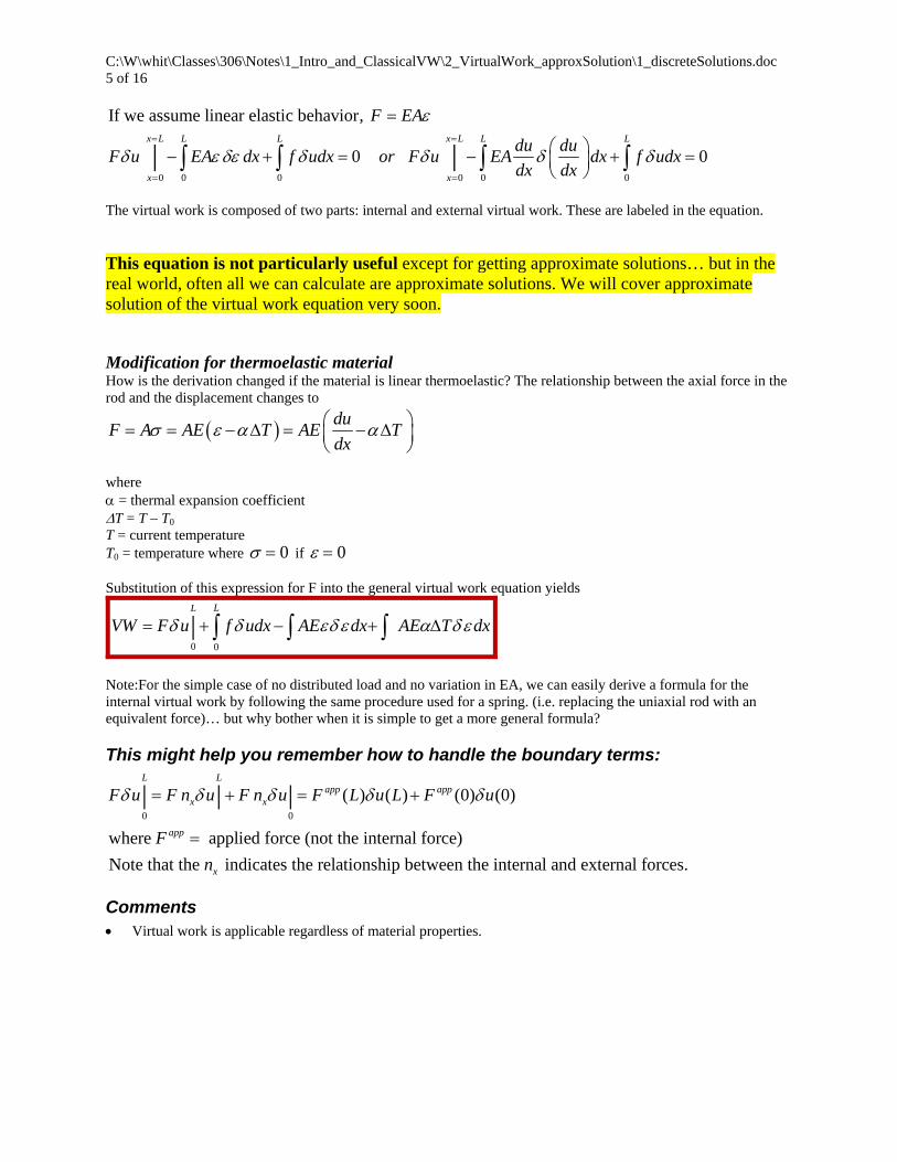
If we assume linear elastic behavior,
0 0| |x L x LL L L L
x x
F EA
du duF u EA dx f udx or F u EA dx f udx
dx dx
The virtual work is composed of two parts: internal and external virtual work. These are labeled in the equation.
This equation is not particularly useful except for getting approximate solutions… but in the real world, often all we can calculate are approximate solutions. We will cover approximate solution of the virtual work equation very soon. Modification for thermoelastic material How is the derivation changed if the material is linear thermoelastic? The relationship between the axial force in the rod and the displacement changes to
duF A AE T AE T
dx
where = thermal expansion coefficient T = T – T0
T = current temperature T0 = temperature where 0 if 0 Substitution of this expression for F into the general virtual work equation yields
0 0
|LL
VW F u f udx AE dx AE T dx
Note:For the simple case of no distributed load and no variation in EA, we can easily derive a formula for the internal virtual work by following the same procedure used for a spring. (i.e. replacing the uniaxial rod with an equivalent force)… but why bother when it is simple to get a more general formula?
This might help you remember how to handle the boundary terms:
0 0
( ) ( ) (0) (0)
where applied force (not the internal force)
Note that the indicates the relationship between the internal and external forces.
| | |L L
app appx x
app
x
F u F n u F n u F L u L F u
F
n
Comments Virtual work is applicable regardless of material properties.
1/3/2012 p. 74 of 112

C:\W\whit\Classes\306\Notes\1_Intro_and_ClassicalVW\2_VirtualWork_approxSolution\1_discreteSolutions.doc 6 of 16
Linear Nonlinear elastic
Nonlinear inelastic
Compare order of derivatives in differential equation versus virtual work equation. What boundary conditions can be specified in the virtual work equation? What boundary conditions can be specified in the differential equation of equilibrium? Question: Why integrate by parts?
1/3/2012 p. 75 of 112

C:\W\whit\Classes\306\Notes\1_Intro_and_ClassicalVW\2_VirtualWork_approxSolution\1_discreteSolutions.doc 7 of 16
Uniaxial Rod with Two Concentrated Loads Two DOF u uB C,
1 1 2
1
1 2
internal
0
external B C
L L L
L
VW F u F u
VW EA dx EA dx
Need to express in terms of uB and uC
Rod 1
1
1
1
internal1 10
1
1
1
B
B
L
BB
B B
u
L
uL
uVW EA u dx
L L
EAu u
L
x, u
A
B
C
E, A E, A F2
L1 L2
F1
1 2
Rod 2
1 2
1
2
2
internal2 2
internal2
1
1
C B
C B
L L
C BC B
L
C B C B
u u
L
u uL
u uVW EA u u dx
L L
EAVW u u u u
L
1 21 2
1 21 2 2
0
Factor out the variations of the unknowns
( ( ) 0
B C B B C B C B
B B C B C C B
EA EAVW F u F u u u u u u u
L L
EA EA EAu F u u u u F u u
L L L
The coefficients of the variations must each be zero. Hence, we obtain two equations.
1 21 2 2
( ) 0 0B C B C B
EA EA EAF u u u and F u u
L L L
Solve these to obtain:
uL
EAF F
uEA
F L F L F L
B
C
11 2
2 2 1 1 2 1
1
b g
b g
1/3/2012 p. 76 of 112

C:\W\whit\Classes\306\Notes\1_Intro_and_ClassicalVW\2_VirtualWork_approxSolution\1_discreteSolutions.doc 8 of 16
What if there had been a distributed load? What would be different? Try adding a spring or thermal load.
Truss Example
1
2
3
60
60 E, A, L
E, A, L
= 30
y, v
x, u
P
L
DOF = u and v at point 2
virtual displacement = u v,
2
1
;
e i e i
i e
VW VW VW VW VW
VW EA ds VW P v
= (Elongation of truss member)/Length
Tension positive
12
32
12
32
1cos sin
1cos sin
1cos sin
1cos sin
u vL
u vL
u vL
u vL
2
2
30 cos .866 cos .75
sin .5 sin .25
1/3/2012 p. 77 of 112
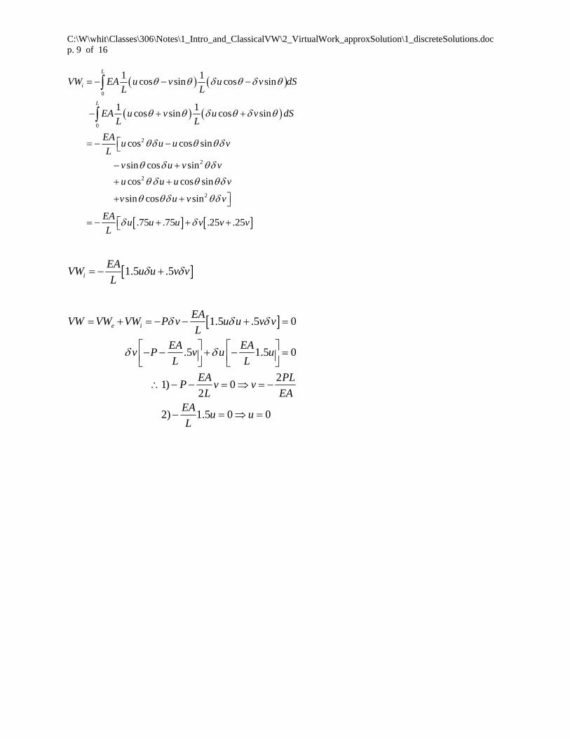
C:\W\whit\Classes\306\Notes\1_Intro_and_ClassicalVW\2_VirtualWork_approxSolution\1_discreteSolutions.doc p. 9 of 16
0
0
2
2
2
2
1 1cos sin cos sin
1 1cos sin cos sin
cos cos sin
sin cos sin
cos cos sin
sin cos sin
.75 .75 .25 .25
L
i
L
VW EA u v u v dSL L
EA u v u v dSL L
EAu u u v
L
v u v v
u u u v
v u v v
EAu u u v v v
L
1.5 .5i
EAVW u u v v
L
1.5 .5 0
.5 1.5 0
21) 0
2
2) 1.5 0 0
e i
EAVW VW VW P v u u v v
LEA EA
v P v u uL L
EA PLP v v
L EAEA
u uL
1/3/2012 p. 78 of 112
C:\W\whit\Classes\306\Notes\1_Intro_and_ClassicalVW\2_VirtualWork_approxSolution\1_discreteSolutions.doc p. 10 of 16
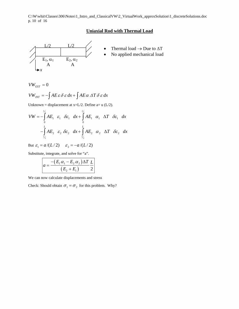
Uniaxial Rod with Thermal Load
L/2 L/2
E1, 1
A E2, 2
A x
Thermal load Due to T No applied mechanical load
dxTAEdxAEVW
VW
INT
EXT
0
Unknown = displacement at x=L/2. Define a= u (L/2).
2 2
2 2
1 1 1 1 1 1
0 0
2 2 2 2 2 2
L L
L L
L L
VW AE dx AE T dx
AE dx AE T dx
But 1 2/( / 2) /( / 2)a L a L
Substitute, integrate, and solve for “a”.
1 1 2 2
2 1 2
E E T La
E E
We can now calculate displacements and stress
Check: Should obtain 21 for this problem. Why?
1/3/2012 p. 79 of 112

C:\W\whit\Classes\306\Notes\1_Intro_and_ClassicalVW\2_VirtualWork_approxSolution\1_discreteSolutions.doc p. 11 of 16
Introduction to Approximate Solution Using Virtual Work (Not to be confused with "only a few mistakes")
x P
E, A are constant Length = L
f = 10x2
How would you obtain an approximate solution of the problem defined by the differential
equation and the BC's? What does “approximate” mean? The following will describe how to obtain an approximate solution of the virtual work equation:
LL
00 0
du du duEA u | f udx EA dx 0
dx dx dx
L
The technique that will be used is known as the “Rayleigh-Ritz Method” (Rayleigh – 1877, Ritz – 1909). The technique was developed because many problems are either impossible or extremely difficult to solve exactly. Step 1 - Assume a solution for u(x) that is expressed in terms of some unknown parameters.
Example: u(x) = a+bx+cx2 Step 2 - Make sure the assumed solution satisfies all kinematic (i.e. displacement) BC's. In
our case, this means 2
x = 0(0) 0 a bx cx | a 0u . Therefore a "valid assumed
solution" is u(x) = bx+cx2
Step 3 - Impose the force boundary conditions in the VW equation. In our case, it is
x = L
duEA | P
dx .
The result of steps 2 and 3 is that L
0
duEA u | P u(L)-0= P u(L)
dx .
What would happen if you tried doing this with the differential equation?
1/3/2012 p. 80 of 112
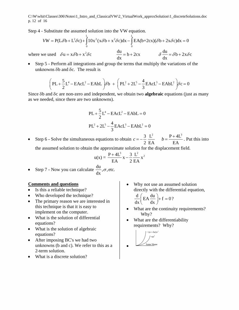
C:\W\whit\Classes\306\Notes\1_Intro_and_ClassicalVW\2_VirtualWork_approxSolution\1_discreteSolutions.doc p. 12 of 16
Step 4 - Substitute the assumed solution into the VW equation. L L
2 2 2
0 0
P(L b L c) 10x (x b x c)dx EA(b+2cx)( b 2x c)dx 0VW
where we used 2 du duu x b x c b 2cx b 2x c
dx dx
Step 5 - Perform all integrations and group the terms that multiply the variations of the unknowns b and c. The result is
4 2 2 5 3 25 4PL L EAcL EAbL b PL 2L EAcL EAbL c 0
2 3
Since b and c are non-zero and independent, we obtain two algebraic equations (just as many as we needed, since there are two unknowns).
4 2
2 5 3 2
5PL L EAcL EAbL 0
24
PL 2L EAcL EAbL 03
Step 6 - Solve the simultaneous equations to obtain 2 33 L P 4L
2 EA EAc b
. Put this into
the assumed solution to obtain the approximate solution for the displacement field. 3 2
2P 4L 3 Lu(x) = x x
EA 2 EA
Step 7 - Now you can calculate du
, ,etc.dx
Comments and questions Is this a reliable technique? Who developed the technique? The primary reason we are interested in
this technique is that it is easy to implement on the computer.
What is the solution of differential equations?
What is the solution of algebraic equations?
After imposing BC's we had two unknowns (b and c). We refer to this as a 2-term solution.
What is a discrete solution?
Why not use an assumed solution directly with the differential equation, d du
EA f 0dx dx
?
What are the continuity requirements? Why?
What are the differentiability requirements? Why?
~ ( )a a x 2
~ax2
Same Shape
1/3/2012 p. 81 of 112

C:\W\whit\Classes\306\Notes\1_Intro_and_ClassicalVW\2_VirtualWork_approxSolution\1_discreteSolutions.doc p. 13 of 16
Summary of Procedure for Using Discrete Version of the Principle of Virtual Work 1. Determine a kinematically admissible assumed solution
Select polynomial series or other approximation with n m unknown coefficients, where n = # term
solution desired and m = number of kinematic constraints.
Impose kinematic constraints. This will reduce the number of unknowns to “n” and result in a
kinematically admissible approximation.
2. Calculate all derivatives and variations.
3. Calculate virtual work = VW = internal externalVW VW
4. Identify simultaneous equations to be solved to determine coefficients in approximation.
Alternatives:
5. Solve equations … now you have the displacement field. This can now be used in calculating the deformed
shape, strains, and stresses.
What are the continuity requirements for the assumed solution? What if there are discontinuities in the problem? Can we use a piecewise solution?
Does not have to satisfy force type boundary conditions! ---the power of this method depends on not having to satisfy them ---it is wrong to say it does
1/3/2012 p. 82 of 112

C:\W\whit\Classes\306\Notes\1_Intro_and_ClassicalVW\2_VirtualWork_approxSolution\1_discreteSolutions.doc p. 14 of 16
Matrix Form of Virtual Work for Rod When we obtained a 2-term approximate solution using virtual work, we had 2 equations. These equations can be expressed in matrix form. (stiffness matrix) * unknowns = (load vector) Except for very simple problems it is very useful to have formulas for calculating the stiffness matrix and load vector “directly”. The derivation of these formulas is as follows. Assumptions Thermoelastic material Distributed load
Concentrated load P at x=x0.
00 0 0
du ( ) 0 where =E
dx
: ( ) but we will write simply with it understood
|L LL
i i i i
VW F u udx A dx P u x T
Approximation u x a f x u a f
that and are functions of xi
i ii i i i i i
u f
Summary
df dfduu a f u a f a a
dx dx dx
We could substitute all of this into the virtual work statement at once, but it will be a little cleaner if we first substitute in the approximation for u and .
00 0 0
0|L LL
Li i
i i i i i i i i
df dfVW F a f a f dx EA a dx EA T a dx P a f
dx dx
We can put all the terms inside of a common summation
000 0 0
i i
000 0 0
( ) 0
Since the a are non-zero and independent, the coefficient of each a must=0
( )
|
|
L LLL
i ii i i i
L LLL
i ii i i
df dfVW a F f f dx EA dx EA T dx Pf x
dx dx
df dfF f f dx EA dx EA T dx Pf x
dx dx
0
This is the set of equilibrium equations that must be satisfied. For the type of problems we are considering in 306,
only the in the third term is a function of the unknowns ia . Let’s substitute the approximation for into the third
term. (Note that I used “j” for the summation index to avoid confusion with the “i” that I used earlier.)
000 0 0
000 0 0
0 ( ) 0
( ) 0
|
|
L LLLj i i
i i j i
L LLLj i i
i i j i
df df dfF f f dx EA a dx EA T dx Pf x
dx dx dx
df df dfF f f dx a EA dx EA T dx Pf x
dx dx dx
Or
1/3/2012 p. 83 of 112
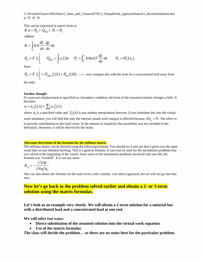
C:\W\whit\Classes\306\Notes\1_Intro_and_ClassicalVW\2_VirtualWork_approxSolution\1_discreteSolutions.doc p. 15 of 16
This can be expressed in matrix form as
0
000 0
( )|
B dist T C
Lj i
LLL
iB i dist i T C i
K a P Q P P
where
df dfK EA dx
dx dx
dfP F f Q f dx P EA T dx P Pf x
dx
Note:
0
( ) (0)|L
B i right i left iP F f P f L P f ------ now compare this with the term for a concentrated load away from
the ends. Further thought If a non-zero displacement is specified as a boundary condition, the form of the assumed solution changes a little. It becomes
0( ) ( )o i iu a f x a f x
where oa is a specified value and 0( )f x is just another interpolation function. If you substitute this into the virtual
work statement, you will find that only the internal virtual work integral is affected because 0oa . The effect is
to provide contributions to the load vector. In the interest of simplicity this possibility was not included in the derivation. However, it will be derived for the beam. Alternate derivation of the formula for the stiffness matrix The stiffness matrix can be derived using the following formula. You should try it and see that it gives you the same result that we just finished deriving. This is a general formula. It can even be used for the mechanism problems that you solved at the beginning of the course. Since most of the mechanism problems involved only one dof, the formula was “overkill”. It is not any more.
2
iji j
VWK
q q
One can also obtain the formula for the load vector with a similar, very direct approach, but we will not go into that now.
Now let’s go back to the problem solved earlier and obtain a 2- or 3-term solution using the matrix formulas. Let’s look at an example very closely. We will obtain a 2-term solution for a uniaxial bar with a distributed load and a concentrated load at one end. We will solve two ways:
Direct substitution of the assumed solution into the virtual work equation Use of the matrix formulas
The class will decide the problem… so there are no notes here for the particular problem.
1/3/2012 p. 84 of 112
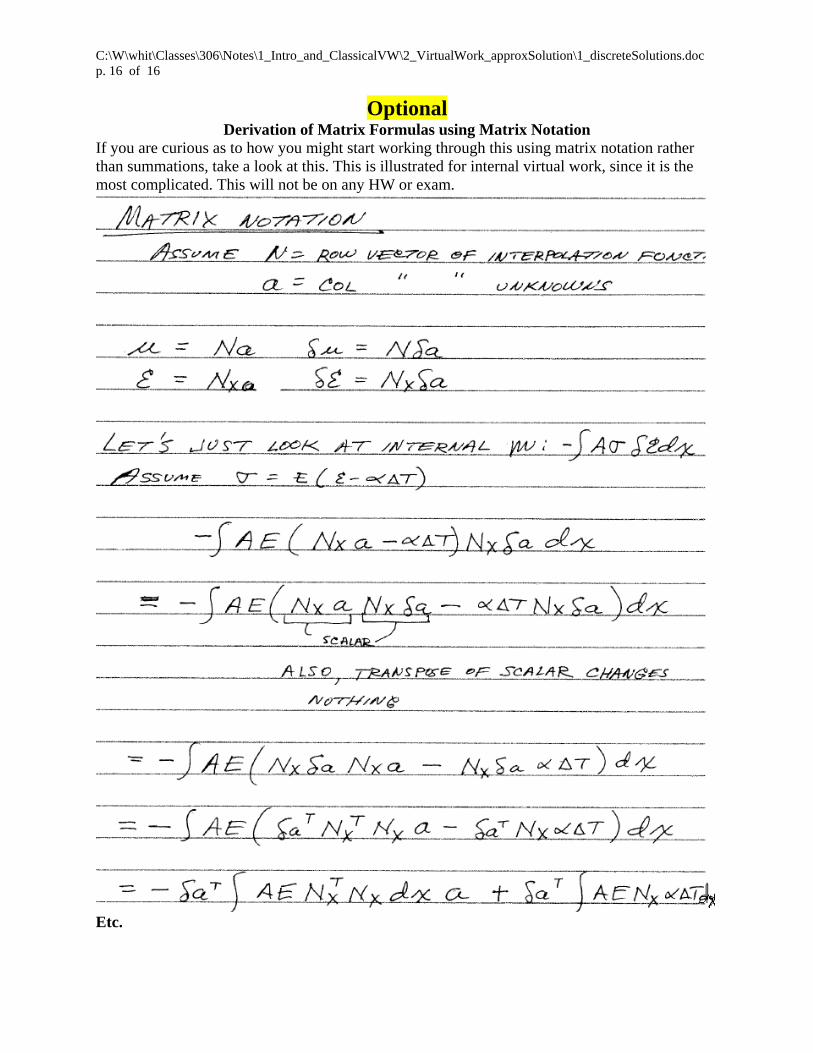
C:\W\whit\Classes\306\Notes\1_Intro_and_ClassicalVW\2_VirtualWork_approxSolution\1_discreteSolutions.doc p. 16 of 16
Optional Derivation of Matrix Formulas using Matrix Notation
If you are curious as to how you might start working through this using matrix notation rather than summations, take a look at this. This is illustrated for internal virtual work, since it is the most complicated. This will not be on any HW or exam.
Etc.
1/3/2012 p. 85 of 112
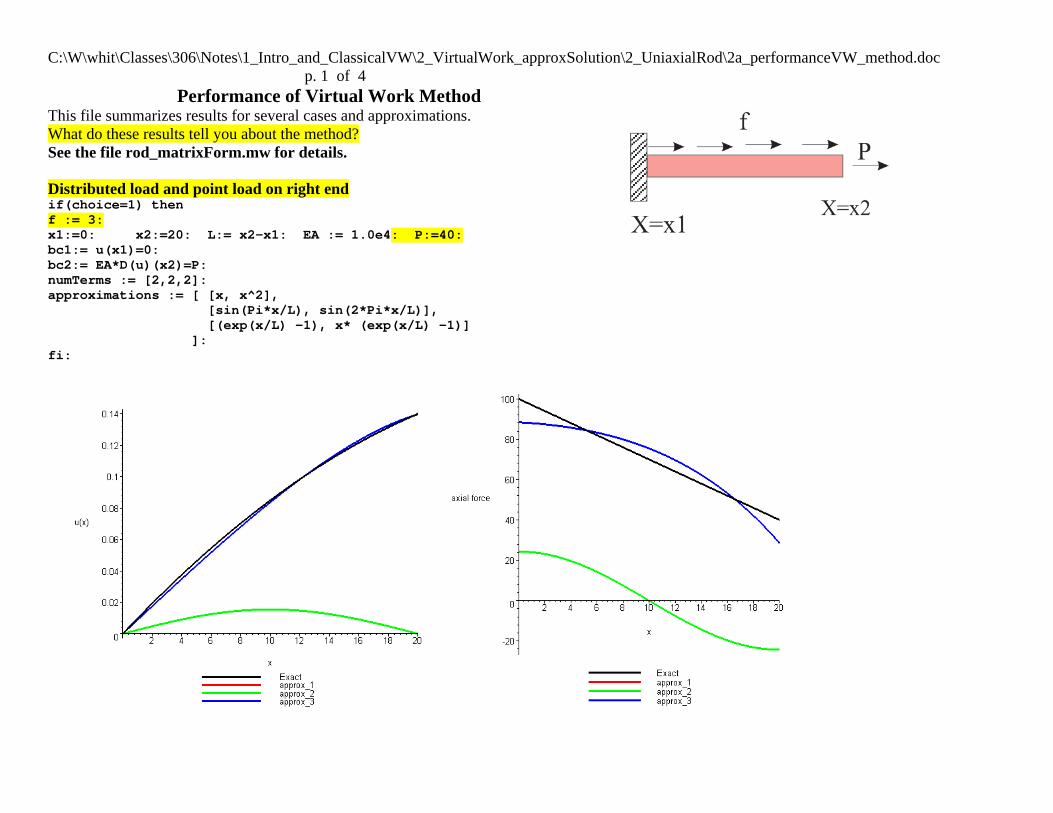
C:\W\whit\Classes\306\Notes\1_Intro_and_ClassicalVW\2_VirtualWork_approxSolution\2_UniaxialRod\2a_performanceVW_method.doc p. 1 of 4
Performance of Virtual Work Method This file summarizes results for several cases and approximations. What do these results tell you about the method? See the file rod_matrixForm.mw for details. Distributed load and point load on right end if(choice=1) then f := 3: x1:=0: x2:=20: L:= x2-x1: EA := 1.0e4: P:=40: bc1:= u(x1)=0: bc2:= EA*D(u)(x2)=P: numTerms := [2,2,2]: approximations := [ [x, x^2], [sin(Pi*x/L), sin(2*Pi*x/L)], [(exp(x/L) -1), x* (exp(x/L) -1)] ]: fi:
1/3/2012 p. 86 of 112

C:\W\whit\Classes\306\Notes\1_Intro_and_ClassicalVW\2_VirtualWork_approxSolution\2_UniaxialRod\2a_performanceVW_method.doc p. 2 of 4 Sinusoidal distributed load and point load on right end if(choice=2) then x1:=0: x2:=20: L:= x2-x1: f := sin(2*Pi*x/(x2-x1)): EA := 1.0e4: P:=40: bc1:= u(x1)=0: bc2:= EA*D(u)(x2)=P: numTerms := [2,2,2]: approximations := [ [x, x^2], [sin(Pi*x/L), sin(2*Pi*x/L)], [(exp(x/L) -1), x* (exp(x/L) -1)] ]: fi:
Distributed load. No point load on right end (If I change the first approximation to have x^3 and x^4, the prediction is much better) if(choice=3) then
1/3/2012 p. 87 of 112
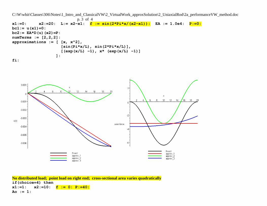
C:\W\whit\Classes\306\Notes\1_Intro_and_ClassicalVW\2_VirtualWork_approxSolution\2_UniaxialRod\2a_performanceVW_method.doc p. 3 of 4 x1:=0: x2:=20: L:= x2-x1: f := sin(2*Pi*x/(x2-x1)): EA := 1.0e4: P:=0: bc1:= u(x1)=0: bc2:= EA*D(u)(x2)=P: numTerms := [2,2,2]: approximations := [ [x, x^2], [sin(Pi*x/L), sin(2*Pi*x/L)], [(exp(x/L) -1), x* (exp(x/L) -1)] ]: fi:
No distributed load; point load on right end; cross-sectional area varies quadratically if(choice=4) then x1:=1: x2:=10: f := 0: P:=40: Ao := 1:
1/3/2012 p. 88 of 112

C:\W\whit\Classes\306\Notes\1_Intro_and_ClassicalVW\2_VirtualWork_approxSolution\2_UniaxialRod\2a_performanceVW_method.doc p. 4 of 4 A := Ao*(1 + (x2-x)^2/(x2-x1) ): E := 1.0E7: EA := E*A: bc1:= u(x1)=0: EAx2 := subs(x=x2,EA): bc2:= EAx2*D(u)(x2)=P: numTerms := [1,2,4]: approximations := [ [x-x1], [x-x1, x*(x-x1)], [x-x1, x*(x-x1),x^2*(x-x1),x^3*(x-x1)] ]: fi:
1/3/2012 p. 89 of 112
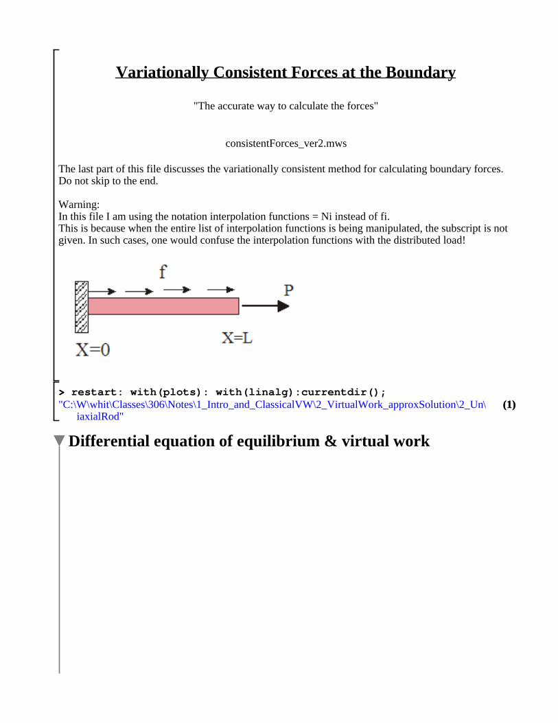
(1)(1)> >
Variationally Consistent Forces at the Boundary
"The accurate way to calculate the forces"
consistentForces_ver2.mws
The last part of this file discusses the variationally consistent method for calculating boundary forces. Do not skip to the end.
Warning:In this file I am using the notation interpolation functions = Ni instead of fi.This is because when the entire list of interpolation functions is being manipulated, the subscript is not given. In such cases, one would confuse the interpolation functions with the distributed load!
restart: with(plots): with(linalg):currentdir();"C:\W\whit\Classes\306\Notes\1_Intro_and_ClassicalVW\2_VirtualWork_approxSolution\2_Un\
iaxialRod"
Differential equation of equilibrium & virtual work
1/3/2012 p. 90 of 112

> >
(2.1.1)(2.1.1)
> >
> >
f :=x^3:P :=5000:L:=20:EA:= 10^6:
Exact solution of differential equation (i.e. determination of u(x))We will use this for evaluating the accuracy of our approximate solution
Integrate differential equation
sol :=dsolve( diff( EA * diff(uGen(x), x), x) + f, uGen(x)):uExact := rhs(sol):print(`The generic solution = `, uExact);
The generic solution = , K1
20000000 x5C_C1 xC_C2
Impose BC's to determine integration constants _C1 and _C2BC's: u(0)=0 and F(L) = P
u0 := subs(x=0, uExact):forceAtL := simplify(subs(x=L,EA * diff(uExact,x) ) );ans := solve( {u0 =0, forceAtL = P}, {_C1, _C2} ):print(`The integration constants are =`, ans);
1/3/2012 p. 91 of 112
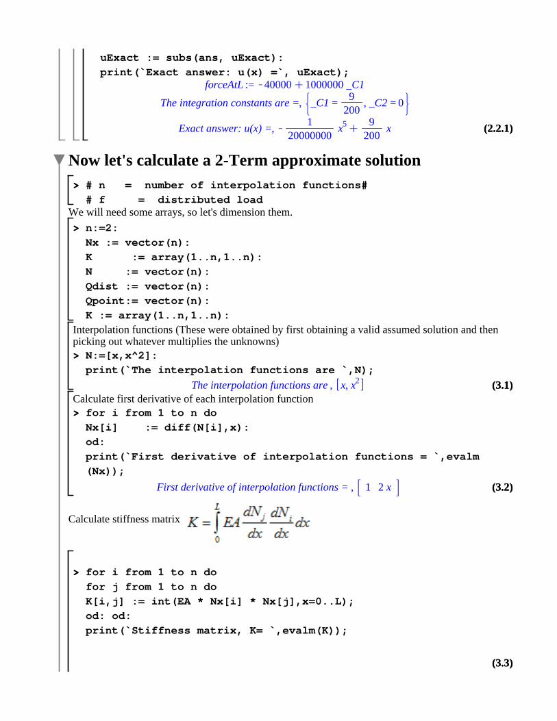
> >
> >
(3.3)(3.3)
> >
> >
(3.2)(3.2)
(3.1)(3.1)
> >
(2.2.1)(2.2.1)
uExact := subs(ans, uExact):print(`Exact answer: u(x) =`, uExact);
forceAtL := K40000C1000000 _C1
The integration constants are =, _C1 =9
200, _C2 = 0
Exact answer: u(x) =, K1
20000000 x5C
9200
x
Now let's calculate a 2-Term approximate solution
# n = number of interpolation functions## f = distributed load
We will need some arrays, so let's dimension them.
n:=2:Nx := vector(n):K := array(1..n,1..n):N := vector(n):Qdist := vector(n):Qpoint:= vector(n):K := array(1..n,1..n):
Interpolation functions (These were obtained by first obtaining a valid assumed solution and then picking out whatever multiplies the unknowns)N:=[x,x^2]:print(`The interpolation functions are `,N);
The interpolation functions are , x, x2
Calculate first derivative of each interpolation functionfor i from 1 to n doNx[i] := diff(N[i],x):od:print(`First derivative of interpolation functions = `,evalm(Nx));
First derivative of interpolation functions = , 1 2 x
Calculate stiffness matrix
for i from 1 to n dofor j from 1 to n doK[i,j] := int(EA * Nx[i] * Nx[j],x=0..L);od: od:print(`Stiffness matrix, K= `,evalm(K));
1/3/2012 p. 92 of 112

(3.3)(3.3)
(3.5)(3.5)
(3.7)(3.7)
> >
> >
> >
(3.6)(3.6)
(3.4)(3.4)
> >
Stiffness matrix, K= ,
20000000 400000000
40000000032000000000
3
Calculate contribution of distributed load
for i from 1 to n doQdist[i] := int(f*N[i],x=0..L ):od:print(`Contribution of distributed load =`, evalm(Qdist) );
Contribution of distributed load =, 64000032000000
3
Calculate contribution of concentrated loads at boundary
The contribution at x=0 is zero , since the displacement is specified. You will note that the interpolation functions evaluate to zero at x=0. That is not accidental.Qpoint := subs(x=L, evalm(P * N) ):print(`The boundary contribution =`, Qpoint);
The boundary contribution =, 100000 2000000
Comment: The contribution of any concentrated load, even if it is not at a boundary is
This is a general formula for any concentrated force.Solve equations to determine unknowns (i.e. the dof):
a := evalm( inverse(K) &* evalm( Qdist + Qpoint) );
a :=53
1000K
11250
Multiply dof with interpolation functions to obtain approximate solution.
uSol_2:=simplify(evalm(a &* N)):print(`Approximate solution: u(x) = `, uSol_2);
Approximate solution: u(x) = ,53
1000 xK
11250
x2
Numerical comparison of exact and approximate solutions
1/3/2012 p. 93 of 112

(4.2.1)(4.2.1)
> >
> >
Displacement and force variation
sol := [uExact, uSol_2]:p := vector(2):p[1] :=plot(sol,x=0..20, color=[black,red],title=`Variation of Displacement`,thickness=[1,3],legend =[`Exact displacement`, `Approximate displacement`]):
strains := map(diff,[ uExact, uSol_2],x): p[2] := plot(EA * strains,x=0..20, color=[black,red],title=`Variation of Axial Force`,thickness=[1,3],legend =[`Exact force`, `Approximate force`]):#display(p);DocumentTools:-Do( %Plot1 =display(p) ):
Exact displacementApproximate
displacement
x0 5 10 15 20
0
0.2
0.4
0.7Variation of Displacement
Exact forceApproximate force
x0 5 10 15 20
10000
20000
30000
40000
50000
Variation of Axial Force
Comments
Note that the displacement prediction is not too bad, but that the internal force calculation has pretty significant error. We do not need the exact solution of the differential equation to know that the errors are large. At the right end the force is supposed to be 5000. Instead, we got 21000.
forceBasedOnDisplacementSolution := subs x = L, EA v
vx uSol_2
forceBasedOnDisplacementSolution := 21000
At the left end, we can determine what the internal force should be by using a free body diagram and summing forces. We will find that the internal force should be
1/3/2012 p. 94 of 112

> >
(4.2.3)(4.2.3)
(4.2.2)(4.2.2)
> >
internalForce_leftEnd :=0
L
f dxCP
internalForce_leftEnd := 45000At the left end the internal force based on the approximate displacement field is
EA v
vx uapprox evaluated at x=0. This gives
forceBasedOnDisplacementSolution := subs(x = 0,EA*diff(uSol_2,x));
forceBasedOnDisplacementSolution := 53000If the displacement field had been exact, the forces would have been calculated correctly.
However, we do have a more accurate way of calculating the forces at the boundaries. It is known as a "variationally consistent" method, because we use the virtual work equation to determine the forces.
Variationally consistent calculation
Let's give it a trySet up the interpolationn:=3:N:= [1,x,x^2]:K := array(1..n,1..n):Nx:= vector(n):
1/3/2012 p. 95 of 112

(4.3.1)(4.3.1)
> >
(4.3.2)(4.3.2)
(4.3.5)(4.3.5)
(4.3.4)(4.3.4)
> >
> >
(4.3.3)(4.3.3)
for i from 1 to n doNx[i] := diff(N[i],x):od:print(`The interpolation functions are`, evalm(N));
The interpolation functions are, 1 x x2
Calculate the stiffness matirx for i from 1 to n dofor j from 1 to n doK[i,j] := int(EA * Nx[i] * Nx[j],x=0..L);od: od:print(`The stiffness matrix =`,evalm(K));
The stiffness matrix =,
0 0 0
0 20000000 400000000
0 40000000032000000000
3
Calculate the contribution due to the distributed load Qdist:=vector(n):for i from 1 to n doQdist[i] := int(f*N[i],x=0..L ):od:print(`Qdist = `,evalm(Qdist) );
Qdist = , 40000 64000032000000
3
Put the values of the dof in a vector. Note that the first dof is zero and the other two were obtained when we solved the problem above.q := [0,a[1], a[2]]:print(`The dof = `, q);
The dof = , 0,53
1000, K
11250
Calculate to obtain
evalm(K&* q-Qdist);
K40000 100000 2000000
From earlier, we had
Hence
1/3/2012 p. 96 of 112

*We obtained the exact solution for the forces at the boundaries from an approximate solution! Do not always count on getting exact forces, but the variationally consistent method is quite powerful and gives more accurate answers than calculating strain, etc..*This technique only gives the internal forces at the two ends... not at any other points.
General formula for calculating boundary forces
This formula is valid not only for uniaxial bars... it also is valid for beams (and other types of structures, including ones we are not covering in 306). We will study beams next. We will not re-derive this technique, because the technique is the same.
This formula is also valid when we use finite elements later in the course. When we use it for finite elements, it is easier to apply (but the theory is the same).
1/3/2012 p. 97 of 112

C:\W\whit\Classes\306\Notes\1_Intro_and_ClassicalVW\2_VirtualWork_approxSolution\3_Beam\3a_beam.doc p. 1 of 15
Euler-Bernouli Beam Theory The sketch below shows a beam. This one happens to be laminated. We will limit our discussion to homogeneous beams, since the points to be made can be illustrated without introducing lamination. y, v z
x, u
b
h
Assumptions/Approximations b and h are constant (we can relax these requirements) Axial displacement u varies linearly in y-direction. Transverse displacement v is constant in y-direction 0y
0y
2, 0hxy y
0xy (typically, the hardest assumption to satisfy)
xf constant in y-direction
For “thin” beams the contributions of xy to strain energy and deformation is negligible.
The Euler-Bernoulli beam theory assumes thin beam behavior. For “thick” beams, the assumption xy =0 can cause large errors. The shear modulus affects how thick a beam
can be and still be considered thin. The lower the shear modulus the smaller the thickness must be for a beam to be considered thin. Composites tend to have a smaller ratio of shear to extensional modulus than homogeneous metals. Hence, the ratio of length to thickness must be larger for a composite beam to behave like a thin beam. As with any elasticity type of problem, there are several categories of equations to be satisfied.
Equilibrium (conservation of linear and angular momentum) Kinematic Constitutive Boundary conditions
What is different in this course is that we express the equilibrium equations in terms of virtual work. As a review, we will begin with a derivation of the differential equation of equilibrium and then derive the virtual work form.
1/3/2012 p. 98 of 112
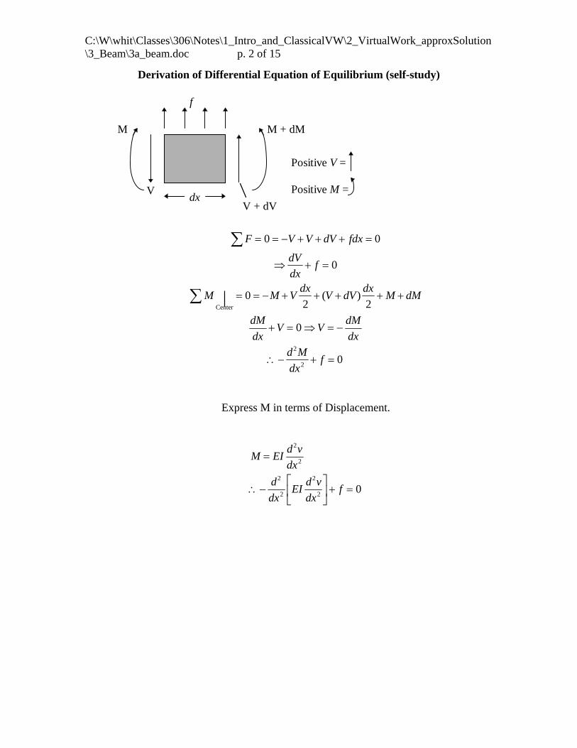
C:\W\whit\Classes\306\Notes\1_Intro_and_ClassicalVW\2_VirtualWork_approxSolution\3_Beam\3a_beam.doc p. 2 of 15
Derivation of Differential Equation of Equilibrium (self-study)
dx
M + dMM
f
V
Positive V =
Positive M =
V + dV
F V V dV fdx
dV
dxf
M M Vdx
V dVdx
M dM
dM
dxV V
dM
dx
d M
dxf
0 0
0
02 2
0
02
2
Center| ( )
Express M in terms of Displacement.
M EId v
dx
d
dxEI
d v
dxf
LNMOQP
2
2
2
2
2
20
1/3/2012 p. 99 of 112

C:\W\whit\Classes\306\Notes\1_Intro_and_ClassicalVW\2_VirtualWork_approxSolution\3_Beam\3a_beam.doc p. 3 of 15
Virtual Work for Flexure of a Beam (one plane only) <<How is the following different from derivation of differential equations of equilibrium?)
M + dM
V + dV
Vdx
f
M Two DOF v and two virtual displacement
,v
d VW v V V dV fdx Vdx
V dVdx
M M dMb g b g LNM
OQP
2 2
d VW
dxv
dV
dxf
dM
dxV
VW vdV
dxf
dM
dxV dx v
dV
dx
dM
dxdx f v V dx
L L
( ) LNM
OQP LNM
OQP
LNMOQP LNM
OQP
LNM
OQP F
HGIKJ z zz
00 0
Integrate by parts
0 0
0
|
|
LL
L
dV d dv dvv dx vV V dx V v V dx
dx dx dx dx
dM d d ddx M M dx M M dx
dx dx dx dx
0
0 |L dv d
VW V v M V dx M dx f v V dxdx dx
VW=2
20
0 |Ldv d v
V v M M dx f vdxdx dx
since
for small rotations and if we assume the transverse shear strain is zerodv
dx
How do we modify this if there is a point load away from ends?
1/3/2012 p. 100 of 112
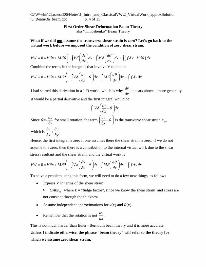
C:\W\whit\Classes\306\Notes\1_Intro_and_ClassicalVW\2_VirtualWork_approxSolution\3_Beam\3a_beam.doc p. 4 of 15
First Order Shear Deformation Beam Theory aka “Timoshenko” Beam Theory
What if we did not assume the transverse shear strain is zero? Let’s go back to the virtual work before we imposed the condition of zero shear strain.
0
0 |L dv d
VW V v M V dx M dx f v V dxdx dx
Combine the terms in the integrals that involve V to obtain
0
0 |L dv d
VW V v M V dx M dx f v dxdx dx
I had started this derivation in a 1-D world, which is why appears above... more generally,
it would be a partial derivative and the first integral would be
.
Since = - for s
dv
dx
vV dx
x
u
y
mall rotation, the term is the transverse shear strain ,
which is .
xy
v
x
v u
x y
Hence, the first integral is zero if one assumes there the shear strain is zero. If we do not
assume it is zero, then there is a contribution to the internal virtual work due to the shear
stress resultant and the shear strain, and the virtual work is
0
0 |L v d
VW V v M V dx M dx f v dxx dx
To solve a problem using this form, we will need to do a few new things, as follows
Express V in terms of the shear strain:
where k = "fudge factor", since we know the shear strain and stress are
not constant through the thickness
xyV GAk
Assume independent approximations for v(x) and (x).
Remember that the rotation is not .dv
dx
This is not much harder than Euler –Bernoulli beam theory and it is more accurate.
Unless I indicate otherwise, the phrase “beam theory” will refer to the theory for
which we assume zero shear strain.
1/3/2012 p. 101 of 112
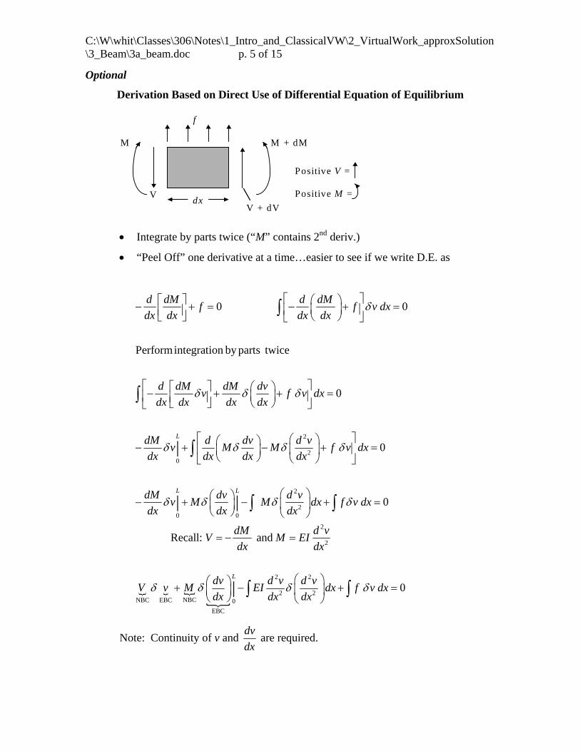
C:\W\whit\Classes\306\Notes\1_Intro_and_ClassicalVW\2_VirtualWork_approxSolution\3_Beam\3a_beam.doc p. 5 of 15
Optional
Derivation Based on Direct Use of Differential Equation of Equilibrium
Positive V = Positive M =
dx
M + dMM
f
V V + dV
Integrate by parts twice (“M” contains 2nd deriv.)
“Peel Off” one derivative at a time…easier to see if we write D.E. as
2
20
0
0 0
Performintegration by parts twice
0
0|
|
L
L
d dM d dMf f v dx
dx dx dx dx
d dM dM dvv f v dx
dx dx dx dx
dM d dv d vv M M f v dx
dx dx dx dx
dM dvv M
dx dx
2
20
2
2
2 2
2 2NBCNBC EBC 0
EBC
0
Recall: and
0
|
|
L
L
d vM dx f v dx
dx
dM d vV M EI
dx dx
dv d v d vV v M EI dx f v dx
dx dx dx
Note: Continuity of v and dv
dx are required.
1/3/2012 p. 102 of 112

C:\W\whit\Classes\306\Notes\1_Intro_and_ClassicalVW\2_VirtualWork_approxSolution\3_Beam\3a_beam.doc p. 6 of 15
The following gives a 1-term solution. Read it on your own. Let’s do a 2-term solution in class.
Modified problem: specify the transverse displacement at x=L to b 5. (Note how the valid assumed solution takes the form
0( ) ( ) ( )i iv x f x a f x )
1-Term Solution
y, v
f
x
x = L
What are the BC’s?
VW for a Beam 2 2
L
2 20
d v d vM V v | f vdx EI dx 0
dx dx
1-Term Solution
2
2 2
#of kinematic constraints 2
start with 3 terms
v a bx cx
dv(0) a 0 (0) b 0 v cx ; v x c
dxv
2 2
2 2
L
0
2
3
2 22
approx
d v d v2 ; 2 c
dx dx
Also, M +V v | 0 Why?
fx cdx EI 2c 2 c dx 0
fc 4EIcL 0
3
f L f Lc v x
12EI 12EI
c
L
Critique this solution……….. How do you critique a solution if you do not have
the exact answer available? Let’s do a 2-term solution… then we can move on to deriving and using the
matrix form.
1/3/2012 p. 103 of 112
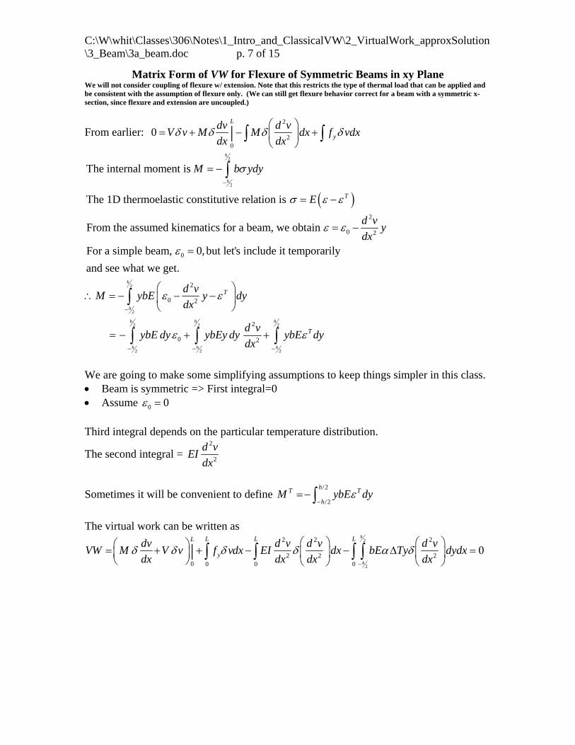
C:\W\whit\Classes\306\Notes\1_Intro_and_ClassicalVW\2_VirtualWork_approxSolution\3_Beam\3a_beam.doc p. 7 of 15
Matrix Form of VW for Flexure of Symmetric Beams in xy Plane We will not consider coupling of flexure w/ extension. Note that this restricts the type of thermal load that can be applied and be consistent with the assumption of flexure only. (We can still get flexure behavior correct for a beam with a symmetric x-section, since flexure and extension are uncoupled.)
From earlier: 2
20
0 |L
y
dv d vV v M M dx f vdx
dx dx
2
2
2
0 2
0
The internal moment is
The 1D thermoelastic constitutive relation is
From the assumed kinematics for a beam, we obtain
For a simple beam, 0,but let's include it tem
h
h
T
M b ydy
E
d vy
dx
2
2
2 2 2
2 2 2
2
0 2
2
0 2
porarily
and see what we get.h
h
h h h
h h h
T
T
d vM ybE y dy
dx
d vybE dy ybEy dy ybE dy
dx
We are going to make some simplifying assumptions to keep things simpler in this class. Beam is symmetric => First integral=0 Assume 0 0
Third integral depends on the particular temperature distribution.
The second integral = 2
2
d vEI
dx
Sometimes it will be convenient to define /2
/2
hT T
hM ybE dy
The virtual work can be written as
2
2
2 2 2
2 2 20 0 0 0
0|h
h
L L LL
y
dv d v d v d vVW M V v f vdx EI dx bE Ty dydx
dx dx dx dx
1/3/2012 p. 104 of 112

C:\W\whit\Classes\306\Notes\1_Intro_and_ClassicalVW\2_VirtualWork_approxSolution\3_Beam\3a_beam.doc p. 8 of 15
0 01
01 1
: ( ) ( ) (The N allows us to handle non-zero specified displacements
... E )
n
i ii
n n
i i i ii i
Assume v x N a N x
Summary
dvv N a N v a N
d
xample?
0
1 1
2 2 22 20
2 2 2 2 21 1
n ni i
i ii i
n ni i
i ii i
dN dN dNdva a
x dx dx dx dx
d N d N d Nd v d va a
dx dx dx dx dx
Note: Obtain the assumed solution for a problem that has specified translation or rotation
and show that it matches the form given by 01
n
i ii
v N a N
.
We could substitute all of this into the virtual work statement at once, but it will be a little cleaner if we first substitute in the approximation for variations only.
2
2
22
2 21 1 1 10 0 0
2
210
|h
h
L LLn n n ni i
i i i y i i ii i i i
L ni
ii
dN d Nd vVW M a V a N f a N dx EI a dx
dx dx dx
d NbE Ty a dydx
dx
We can put all the terms inside of a common summation
2
2
2 22
2 2 20 0 0 0
0|h
h
L L LLi i i
i i y i
dN d N d Nd vVW a M V N f N dx EI dx bE Ty dydx
dx dx dx dx
i iSince the a are non-zero and independent, the coefficient of each a must=0
2
2
2 22
2 2 20 0 0 0
0|h
h
L L LLi i i
i y i
dN d N d Nd vM V N f N dx EI dx bE Ty dydx
dx dx dx dx
This is the set of equilibrium equations that must be satisfied. For the type of problems we are considering in 306, only the “v” in the third term is a function of the unknowns ia .
Let’s substitute the approximation for “v” into the third term. (Note that I use “j” for the summation index to avoid confusion with the “i” that I used earlier.)
2
2
22 2 2 20
2 2 2 2 210 0 0 0 0
0|h
h
L L L LL nji i i i
i y i jj
d NdN d N d N d N d NM V N f N dx EI dx EI a dx bE Ty dydx
dx dx dx dx dx dx
Or
1/3/2012 p. 105 of 112

C:\W\whit\Classes\306\Notes\1_Intro_and_ClassicalVW\2_VirtualWork_approxSolution\3_Beam\3a_beam.doc p. 9 of 15
2
2
22 2 2 20
2 2 2 2 210 0 0 0 0
0|h
h
L L L LL nji i i i
i y i jj
d NdN d N d N d N d NM V N f N dx EI dx a EI dx bE Ty dydx
dx dx dx dx dx dx
This can be expressed in matrix form as
.
2 2
2 200
0
2 20
. 2 20
|
dist thermal spec disp
L Lj i i
i
L
dist y i
Li
spec disp
K a P Q Q Q
where
d N d N dNK EI dx P M V N
dxdx dx
Q f N dx
d N d NQ EI dx
dx dx
2
2
2
20
h
h
Li
thermal
d NQ bE Ty dydx
dx
Comments
What if there were also concentrated loads between the ends?
Hint: Start with first equation: 2
20
0 |L
y
dv d vV v M M dx f vdx
dx dx
Just add virtual work due to concentrated load and proceed… just adds another term. However, the results will likely not be very good, since a concentrated force = a discontinuity.
Easy to show that the coefficient matrix can be calculated from 2
iji j
VWK
q q
0 00 0 0
L 0 L 0
The boundary load term
M ,M , V ,V = applied moments and shears, not internal ones!!!
| | | | |L
i i ii L L i i
L L
dN dN dNP M V N M M V N V N
dx dx dx
Why? What is the variationally consistent method for getting boundary forces? Can you give any physical interpretation to the matrix formulas?
1/3/2012 p. 106 of 112

C:\W\whit\Classes\306\Notes\1_Intro_and_ClassicalVW\2_VirtualWork_approxSolution\3_Beam\3a_beam.doc p. 10 of 15
Examples
etc. Possible modifications Remove the specified rotation v’(L)=r Add thermal loads Shift coordinate system Remove spring Other study questions
Compare the beam matrix formulas with those for a uniaxial bar. Students design the problem & we work it out.
1/3/2012 p. 107 of 112
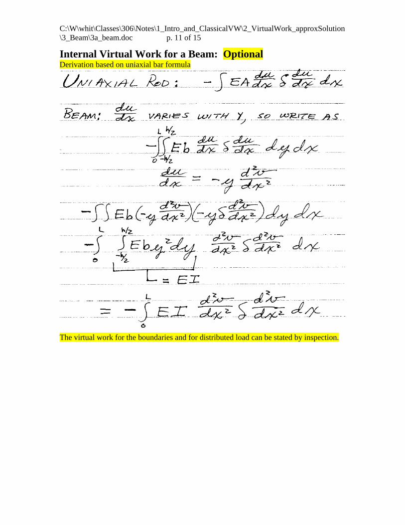
C:\W\whit\Classes\306\Notes\1_Intro_and_ClassicalVW\2_VirtualWork_approxSolution\3_Beam\3a_beam.doc p. 11 of 15
Internal Virtual Work for a Beam: Optional Derivation based on uniaxial bar formula
The virtual work for the boundaries and for distributed load can be stated by inspection.
1/3/2012 p. 108 of 112
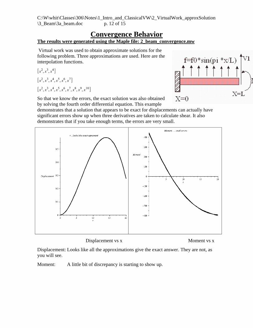
C:\W\whit\Classes\306\Notes\1_Intro_and_ClassicalVW\2_VirtualWork_approxSolution\3_Beam\3a_beam.doc p. 12 of 15
Convergence Behavior The results were generated using the Maple file: 2_beam_convergence.mw
Virtual work was used to obtain approximate solutions for the following problem. Three approximations are used. Here are the interpolation functions.
So that we know the errors, the exact solution was also obtained by solving the fourth order differential equation. This example demonstrates that a solution that appears to be exact for displacements can actually have significant errors show up when three derivatives are taken to calculate shear. It also demonstrates that if you take enough terms, the errors are very small.
Displacement vs x Moment vs x
Displacement: Looks like all the approximations give the exact answer. They are not, as you will see.
Moment: A little bit of discrepancy is starting to show up.
1/3/2012 p. 109 of 112

C:\W\whit\Classes\306\Notes\1_Intro_and_ClassicalVW\2_VirtualWork_approxSolution\3_Beam\3a_beam.doc p. 13 of 15
Shear: Now there is some significant error showing up for the lowest order approximation
Error in satisfying 4th order differential equation of equilibrium Error for just the most accurate approximation The most accurate approximation is very accurate!
1/3/2012 p. 110 of 112
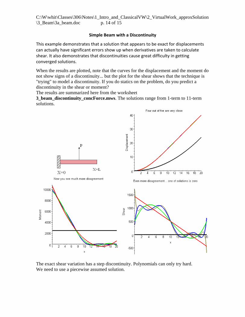
C:\W\whit\Classes\306\Notes\1_Intro_and_ClassicalVW\2_VirtualWork_approxSolution\3_Beam\3a_beam.doc p. 14 of 15
Simple Beam with a Discontinuity
This example demonstrates that a solution that appears to be exact for displacements can actually have significant errors show up when derivatives are taken to calculate shear. It also demonstrates that discontinuities cause great difficulty in getting converged solutions.
When the results are plotted, note that the curves for the displacement and the moment do not show signs of a discontinuity... but the plot for the shear shows that the technique is "trying" to model a discontinuity. If you do statics on the problem, do you predict a discontinuity in the shear or moment? The results are summarized here from the worksheet 3_beam_discontinuity_concForce.mws. The solutions range from 1-term to 11-term solutions.
The exact shear variation has a step discontinuity. Polynomials can only try hard. We need to use a piecewise assumed solution.
1/3/2012 p. 111 of 112

C:\W\whit\Classes\306\Notes\1_Intro_and_ClassicalVW\2_VirtualWork_approxSolution\3_Beam\3a_beam.doc p. 15 of 15
Piecewise Solution This summarizes the results from the file beam_discontinuity_piecewise.mws The exact shear variation has a step discontinuity. Polynomials can only try hard, as we saw in the previous solutions. We need a piecewise solution. If we assume a piecewise cubic approximation that satisfies the continuity requirements, then we will obtain the exact solution. A cubic approximation was assumed for each piece. Continuity of v(x)
and dv
dxwas enforced. Here are the results.
Obtaining a piecewise solution takes some effort. Doing it for complex problems requires help from the computer. Complexity arises due to various causes, including shape of the structure, variation of the material properties (e.g. composites), and the boundary conditions. We need a systematic way to perform piecewise analysis. For some decades now, the best way to perform piecewise analysis has been the Finite Element Method (FEM). That is our next topic.
1/3/2012 p. 112 of 112


![#] +e A ) - 日本弁護士連合会│Japan Federation of … ý Â Â Ë Â Â Ä Â Â Â Å 1 ý Â Â Ë Â Â Ä Â Â Â Å 5U ÊKS 1 ý Â Â Ë Â Â Ä Â Â Â Å1 ý Â](https://static.fdocuments.net/doc/165x107/5ce9840888c993c0208d8cce/-e-a-japan-federation-of-y-a-a-e-a-a-ae.jpg)


