Virginia Tech · THE REACTION OF ORTHO-POSITRONIUM WITH NITROAROMATICS VIA COMPLEX FORMATION by...
197
THE REACTION OF ORTHO-POSITRONIUM WITHNITROAROMATICS VIA COMPLEX FORMATION by William Juul Madia Dissertation submitted to the Graduate Faculty of the Virginia Polytechnic Institute and State University in partial fulfillment of the requirements for the degree of DOCTOR OF PHILOSOPHY APPROVED: in Chemistry Hii.ns J. A-bhe, Chairman John G. Mason Michael A. Ogliaruso John C. Schug Jimmt W. Viers February, 1975 Blacksburg, Virginia
Transcript of Virginia Tech · THE REACTION OF ORTHO-POSITRONIUM WITH NITROAROMATICS VIA COMPLEX FORMATION by...

THE REACTION OF ORTHO-POSITRONIUM
WITH NITROAROMATICS
VIA COMPLEX FORMATION
by
William Juul Madia
Dissertation submitted to the Graduate Faculty of the
Virginia Polytechnic Institute and State University
in partial fulfillment of the requirements for the degree of
DOCTOR OF PHILOSOPHY
APPROVED:
in
Chemistry
Hii.ns J. A-bhe, Chairman
John G. Mason Michael A. Ogliaruso
John C. Schug Jimmt W. Viers
February, 1975
Blacksburg, Virginia

ACKNOWLEDGEMENTS
The author wishes to express his gratitude and appre-
ciation to Dr. Hans J. Ache, his research advisor, whose
helpful comments and critical evaluations of this work
have added greatly to it.
Special thanks are extended to the other members of
his research committee:
Dr. John C. Schug, for his general advice through-
out. His guidance concerning the quantum mechanical calcul-
lations made them possible;
Dr. John G. Mason, for his interest and aid in
resolving the kinetic difficulties that arose during this
work;
Dr. Michael A. Ogliaruso, whose knowledge of
organic chemistry helped to bypass many problems;
Dr. Jimmy W. Viers, for assisting in the computer
programming used throughout this research.
He wishes to acknowledge Dr. Alan Nichols for providing
some of the data used here and also the Atomic Energy
Commission for providing financial aid.
He would like to thank the Chemistry Department's
glassblowing and electronic shops for their assistance and
Mrs. Doris Smith for typing this manuscript.
The author dedicates this dissertation to his wife,
Audrey, for without her it would not have been possible.
ii

TABLE OF CONTENTS
ACKNOWLEDGEMENTS • • . . . . . . . . . . . . . . . . LIST OF FIGURES
LIST OF TABLES
INTRODUCTION . .
. . . . . . . . . . . . . . . . . . . . . . .
. . . . . . . . . .
CHAPTER 1. REVIEW OF BASIC PRINCIPLES
A.
B.
c. D.
E.
The Positron
Positron Decay
. . . . . . . . . . . . . . . . . . . . . . . . . . . . .
Positron Annihilation.
Positronium. . . . . . . . . Quenching •
CHAPTER 2 . EXPERIMENTAL METHODS
A. Introduction . . . . . . . . . . . . . . . B. Positron Sources . . . . . . . . . . . . . c. Fast-Slow Delayed Coincidence Counting
D.
E.
Positron Lifetime Spectra •.
Sample Preparation and Degassing
F. Solvents and Solutes . . . . . . . . . . . CHAPTER 3. CHEMICAL REACTIONS OF ORTHO-POSITRONIUM
A. Diamagnetic Quenchers . . . . . . . . B. Conjugation Effects • • . . • . • . . . . . c. Temperature Effects . . . . . . . . . . . . D. Solvent Effects . . • . . . . . . . • . . . E. Correlations • • • . • . • • . . • • . . .
iii
Page
ii
vi
ix
1
3
4
7
10
17
29
30
33
37
43
49
53
57
62
81
86

iv
CHAPTER 4. POSITRON AND POSITRONIUM COMPLEXES
A. Introduction
B. Hartree-Fock Theory
c. Approximations and Parameterization
D. Results . . . . . . . . . . . . . . . . .
CONCLUSIONS
Summary A.
B. Future Possibilities.
REFERENCES
APPENDIX I. Data Tables
A. Rate Constants for the Reaction of o-Ps with Aromatic Nitro Compounds in Benzene
Page
89
92
96
100
112
113
115
at 295°K. • . . • . . . • . • • • 120
B. Rate Constants for the Reaction of o-Ps with Aliphatic Nitro Compounds in Benzene at 2950K . . . . . . . . . . . . • • . . . 128
C. Temperature Dependence of the Observed Rate Constants for the Reaction of o-Ps with Substituted Nitrobenzenes . . . • 129
D. Temperature Dependence of the Observed Rate Constants for the Reaction of o-Ps with Solvents and Weakly Reactive Compounds • • • . . . . . • . • • 134
E. Thermodynamic Data for the Reactions of o-Ps . . . . . . . . . . . . . . 136
V
APPENDIX II. Computer Programs
A. Introduction •.•
VITA
B.
c. D.
E.
F.
SLOW RATE Program ••.
ARRHENIUS Program ..•••
HAMMETT Program . . . . . . . . . . . PSCF Subroutines . . . . . . . . . . . . . PAL Program . . . . . . . . . . . . .
. . . . . . . . . . . . . . . . . . . . . . .
Page
137
138
141
143
146
163
186

Figure
1.
2.
LIST OF FIGURES
Energy Spectrum of Positrons Emitted from Sodium-22 lfrom Ref. 4} ..•.••..•
Some Physical Properties of Para- and Ortho-Positronium... . • . .
3. (a) Energy Diagram of the Ore Gap and (b) Hypothetical Positronium Formation
Page
6
12
Probability in Gaseous Argon (from Ref. 15) • 16
4. Lattice Potential as Described by the "Free Volume Model" (from Ref. 17) . . • • • 21
5. (a) Angular and (b) Momentum Distributions of the Annihilating Photons . . • . . . • . • 23
6. Computed and Experimental Momentum Distributions for Decane (from Ref. 25)
7. Positron and Positronium Decay in Water (from Ref . 2 O ) • • • • • • • • • • • • •
8. Decay Scheme of Sodium-22 (from Ref. 30)
9.
10.
Simple Fast - Slow Timing System
Typical Positron Lifetime Spectrum
11. Typical Calcomp Plot of the Lifetime Data
12. Prompt Spectrum of Cobalt-60
13. Sample Tube Used for Variable Concentration
26
27
31
34
38
40
42
Experiments . . . . . . . . . . . . • . • . • 44
14.
15.
16.
17.
Degassing Bulb and Sample Tube Used for Variable Temperature Experiments ..•
Experimental Arrangement Used for Low Temperature Lifetime Measurements ..
Experimental Arrangement Used for High Temperature Lifetime Measurements •••
~2 versus Nitrobenzene Concentration in Benzene . . . . . . . . . . . . . . . .
vi
46
50
51
58

vii
Figure
18. Steric Interactions that Force the Nitro Group out of the Plane of the Ring Cause a
Page
Reduction in the Rate Constants . . . . . . . 60
19. Nitro Compounds in Which the Nitro Group is not Attached to a Conjugated System React Slowly with Ortho-Positronium. . . . . . 61
20. Effect of Conjugation on Positronium Rate Constants 63
21. A2 versus T(°C) in Toluene 65
22. Arrhenius Plots for the Reaction of Ortho-Positronium with 9.77mM Nitrobenzene in Toluene (o) and Pure Toluene (o) . . . . . . 66
23. Arrhenius Plots for the Reaction of Ortho-Positronium with Various Nitroaromatics in Toluene . . . . . . . . . . . . . . . . . 67
24. Log (Transmission Coefficient) versus Positronium Energy for Three Different Potential Barriers ......... .
25. Typical Arrhenius Plot for the Reaction of Ortho-Positronium with Nitroaromatics
71
Showing the Thermodynamic Parameters 75
26. Potential Energy Surface for Ortho-Positronium Reacting with a Nitroaromatic Molecule....... 76
27. Arrhenius Plots for the Reaction of Ortho-Positronium with p-Benzoquinone, 2,6-Dimethylnitrobenzene, Benzonitrile and 2-Nitropropane in Toluene . . . . . . . . . . 80
28. Arrhenius Plots for the Reaction of Ortho-Positronium with Nitrobenzene, p-Dinitro-benzene and p-Nitroanisole inn-Heptane . . . 82
29. Arrhenius Plots for the Reaction of Ortho-Positronium with Nitrobenzene, p-Dinitro-benzene and p-Nitroanisole in n-Pentanol 83

viii
Figure
30. Arrhenius Plots for the Reaction of Ortho-Positronium with Nitrobenzene in (0) Toluene,
Page
CO) n-Heptane and (A) n-Pentanol. . . . . . . 85
31. Hammett Plot for the Reaction of Ortho-Positronium with Substituted Nitroaromatics in Toluene at -260C . . . . . . . . . . . 88
32. Variation in Positron Binding Energy in Nitrobenzene with k(+). Koopman's Theorem Estimate CO) and Change in Energy Directly Calculated (6) for the Complex ..... .
33. Profiles of Electronic Total Charge and Pi-Charge for Aniline, Before(-) and After · (-·~) Positron Addition. The Position of the Highest Positron Density (not to scale)
104
is Indicated in the N-H Bond ......... 108

LIST OF TABLES
Table
I. Average Quenching Cross Sections (from Ref. 21) . . • .
II. Thermodynamic Data for the Reactions of
Page
19
o-Ps in Toluene . . . . . . . . . • . 77
III. Thermodynamic Data for the Reactions of o-Ps inn-Heptane and n-Pentanol . . . 84
IV. Positron and Positronium Binding Energies, a. u. k ( +) = 2 / 3 . . . . . . . . . . . . . 102
V. Positron and Positronium Binding Energies, a.u. k(+) = 3/4 . . . . . . . • . . . 103
VI. Calculated Total Charge Densities for Aniline and a Positron-Aniline Complex
(+) -k - 3/4 . . • • . . . . . . . . . . 107
ix

INTRODUCTION
The chemical consequences of a nuclear transformation
such as electronic excitation, ionization, and bond clea-
vage allow one to study the effect that such an event has
on a particular system. This area is generally referred to
as nuclear or radiation chemistry. However, there are
certain nuclear transformations that are directly influenced
by the physical and chemical nature of their environment.
The two most notable of these are the Mtlssbauer effect and
positron annihilation. The study of these types of pheno-
mena cannot be classified as the chemical effect of a
nuclear transformation, but rather as the chemical effect
on it. The physical and chemical properties of a system
alter the rate of positron annihilation and allow the
positron to be used as a probe of its environment. For
example, recent work in this area has used the positron to
measure the electron momentum distributions in certain
aliphatic liquids. It is also applicable to the solid
state where positron lifetimes have been useful in estima-
ting the concentration of lattice defects in semi-conductors.
The positron itself is a stable particle, but life in
ore's antimatter world is quite short, typically a fraction
of a nanosecond in the condensed phase. By forming a bound
state with an electron whose spin is triplet relative to
1

2
the positrons' (ortho-positronium), the positron may exper-
ience a tenfold enhancement in its lifetime.
A rapid reaction in solution has previously been
observed between ortho-positronium and certain diamagnetic
organic molecules such as nitroaromatics and quinones.
They react rapidly with second-order rate constants
typically three orders of magnitude greater than most
diamagnetic compounds.
The focus of this research is to determine the mechan-
ism by which ortho-positronium reacts with a certain class
of compounds, the nitroaromatics, and to evaluate any of
the pertinent conditions necessary for this process.
Determining the nature of this process becomes
possible by studying the variation in the positron life-
time distribution on dissolution of small amounts of these
compounds in suitable solvents. The role that substituents
play will be examined from both a steric and reactivity
viewpoint. Investigating the temperature dependence of
these reactions will also be helpful. Quantum mechanical
calculations will be performed to study the stability of
positron and positronium complexes with diamagnetic organic
molecules.

REVIEW OF BASIC PRINCIPLES
A. The Positron
One of the most interesting consequences of the theory
of relativity is the division of the universe into matter
and anti-matter. Dirac 1 has shown by purely theoretical
arguments that the relativistic wave equation for a free
electron has both positive and negative energy solutions.
The magnitude of these solutions is at least m c2 , where e m is the mass of the electron and c is the speed of light. e
Instead of disregarding the negative solution, he proposed
that it corresponded to a particle with a mass equal to
that of an electron but carrying the opposite charge -- a
positron. Two years later, Anderson 2 discovered the posi-
tron in cloud chamber tracks of cosmic radiation.
The positron states can be intuitively understood in
terms of the "theory of holes." Since electrons are obser-
ved only in positive energy states, the theory requires
that the negative energy states be completely filled with
electrons. 2 A photon with energy greater than 2 m c could e raise an electron from its negative energy state to a
positive one. The "hole" created by this transition in
the "sea" of electrons would behave as a positron in that
it is defined to have negative energy, negative momentum,
and spin opposite to the electron.
3

4
There is a second interpretation of the negative
energy solution which is equally valid and does not require
an unobservable "sea" of electrons. The positron~ instead
of being a negative energy "hole," can be described as an
electron moving backwards in time. 3 At the present level
of our understanding, the latter interpretation has no
physical meaning.
B. Positron Decay
The emission of a positron from a radioactive nucleus
is referred to as positron decay. It occurs in nuclei that
are proton rich in relation to their most stable isobars.
The creation of a positron arises from the transformation
of a proton, p, within the nucleus into a neutron, n, a
positron, S+, and a neutrino, v, with an accompaning de-
crease in the atomic number of the parent nucleus by one
unit.
p ( 1)
The positron cannot exist within a nucleus, because of
difficulties arising from the considerations of angular
momentum conservation, and is emitted. Once the positron
has left the nucleus, it is repelled by the Coulombic
interaction between itself and the positively charged
nucleus. The release of binding energy during positron

5
decay along with the Coulomb effect cause the positron to
possess a considerable amount of kinetic energy. This may
range from a few hundred keV up to several MeV.
The parent and daughter nuclei are in definite energy
states for positron decay. Energetically, in order for
positron decay to take place, the atomic mass of the parent
nucleus, M, must be greater than the sum of the rest mass-P es of two beta particles and the atomic mass of the daugh-
ter nuclei, Md.
> + 2m e (2)
A neutrino is emitted simultaneously with the positron.
Therefore, the energy spectrum of emitted positrons is
continuous rather than having a discrete value. The posi-4 tron energy spectrum for sodium-22 is shown in Figure 1.
The maximum energy, also referred to as the end-point
energy, is 0.544 MeV. In general, the maximum number of
positrons emitted in the energy distribution occurs at one-
third of the end-point energy. The remaining energy is
divided between the recoil energy of the daughter nucleus
and the neutrino energy.
The elementary theory of beta decay, according to the
basic transformations involved, was first given by Fermi. 5
His descriptive ideas gave satisfactory explanations for
the shapes of beta particle energy spectrums, half-lives,

{fJ .µ ·r-1 C: ;::s
:>. 1-i ro 1-i .µ •r-1 ,.Q 1-i ro
~ "d --,,...._ 1-i <ll
,.Q E ;::s z
'--' "d
0.0 0.1
Maximum
0.2 0.3 0.4 Positron Energy, MeV
End-Point Energy
0.5 0.6
Figure 1. Energy Spectrum of Positrons Emitted from Sodium-22. ( from Ref . 4 )
CT')

7
etc. A more modern theorr, which takes into account the
nonconservation of parity, has been developed by using
relativistic quantum mechanics and was introduced by Lee 6 and Yang.
Positrons, like all charged particles, lose their
energy while passing through matter. Their interactions
can induce ionizations and excitations in the stopping
medium. Energy losses due to bremsstrahlung dominate only
at higher energies. 7 Tao and Green have estimated that a·
high energy positron interacting with a dense material
such as water will be slowed down to the first ionization
energy of water in 7 psec. The total time needed to therma-
lize the positron was roughly estimated to be 100 psec.
The interactions of positrons with matter are difficult
to study at very low energies because of the competing
process of mass annihilation whose cross-section is
greatest for thermalized positrons.
C. Positron Annihilation
Annihilation is an event unique to matter-anti-matter
pairs such as the electron-positron. However, it has been
shown by Goldanskii 8 that fewer than five percent of the
positrons emitted into a condensed medium will annihilate
during the slowing down process. According to the theory
of positron annihilation, 9 one, two, or three photons may
be emitted as the result of a collision between a positron

8
and an electron. Xf the two ~articles meet with their
spins antiparallel, two photon emission results. Two
photon emission is forbidden for collisions where the two
particles meet with their spin parallel and three photons
are emitted. Emission of a single photon requires that a
third body, M, be present to absorb the recoil momentum of
the annihilation photon.
e + M y + M (3)
In order to be complete, it should be noted that if two
such bodies, M, are present, annihilation may occur without
the creation of electromagnetic energy.
e + 2M -+ 2M (3a)
The probability of such an occurance is very small and it
has never been observed.
Goldanskii has characterized the three basic mechanisms
by which slow-positrons are annihilated. 8
First, annihilation as "free" positrons in collisions
with electrons of their surroundings.
The cross section for the two photon annihilation of a
positron and an electron, cr2y, was first calculated by
Dirac. 1 He assumed in the calculation, that the electron
of the annihilating pair was at rest. The velocity, v, of
thermal positrons is small (6.6 x 106 cm/sec) compared to
the speed of light and the equation reduces to

=
or
=
9
rrr~ c/v
rrr2c = constant 0
where r = 2.8 x 10- 13 cm is the classical radius of a 0
beta particle.
(4)
(4a)
The two gamma annihilation rate in a multi-electron
system is
= = (5)
where pis the density, N is Avargadro's number, Mis the 0
molecular weight, and ZEFF is the effective number of
electrons seen by the positron (usually this is taken to
be the number of valence electrons). The annihilation
rate in water, assuming ZEFF= 8, is calculated at 2.2
nsec-l and corresponds to a free positron lifetime of 0.46
nsec. This value agrees very well with experimental re-
sults.10 Annihilation rates in the gas phase are usually
two to three orders of magnitude less, due to lower den-
sities.
The triplet interaction usually results in three
photon emission. Ore and Powe11 11 in 1949 were the first
to correctly calculate the ratio of two photon to three
photon annihilation rates as 1115. The much lower triplet
rate, AT' is caused by the multiple character of the three

10
quantum process. The ratio of the cross sections for these
two modes of decay is one-fourth the ratio of the annihila-
tion rates (seep. 13). Sununarizing,
= 1115 = 372 (6)
A second channel of annihilation involves the binding
of a positron to a multi-electron system. This should
cause polarization of the electron shells and subsequent
formation of positron atomic or molecular orbitals. Much
theoretical work in this area is being performed and
Chapter 4 of this work deals with this subject.
D. Positronium
The most widely studied interaction of slow positrons
with matter is the formation of positronium, Ps, a hydrogen-
like bound state of a positron and an electron. This spe-
cies was proposed by Mohorovicic in 1934 12 to account for
the unusual emission spectra of some nebulae. The ioniza-
tion potential of ortho-positronium was calculated to be 13 6.77 eV by Ruark, and he also proposed the name positron-
+ -ium for thee e atom.
In order to treat positronium as the structural
analogue of hydrogen, the reduced mass of hydrogen, µH ~ me'
must be replaced by the reduced mass of the positronium
atom, µPs = me/2. The Bohr radius, ~s' is 1.06 i, twice

11
that of hydrogen, and the first ionization potential,
binding energy, is half as great in positronium as in
hydrogen,
The two ground, n = 1, spin states of positronium are
the singlet, para-positronium (p-Ps) and the triplet, ortho-
positronium (o-Ps). Figure 2 illustrates both forms and
lists some of their characteristics. The average lifetime
of these two atoms in free space can be calculated from
the rates of singlet and triplet annihilation given in
Eq, (5) and (6). To do this, the factor, pN0 ZEFF/M, must
be replaced by the density of the electron wave function
at the positron, lw(o)j 2 . Eq. (5) now becomes
(7)
In a free ground-state atom of positronium
I 12 3 2 2 3 ~(o) = (1/n~s) = (1/n)(µPse /~) =
23 -3 2.68 x 10 cm
and therefore
= 0.125 nsec (8)
for a para-positronium atom in free space. Para-positronium
has a shorter lifetime than that of free positrons in most

N N (-)9 $+) s
Para-Positronium Singlet state 1s
s
Spins are antiparallel Magnetic poles are parallel Disintegrates into 2 photons Mean-life= 0.125 nsec
4+) s (-)9
Ortho-Positronium Triplet State 3s Spins are parallel
s
Magnetic poles are antiparallel Disintegrates into 3 photons Mean-life= 140 nsec
Figure 2. Some Physical Properties of Para- and Ortho-Positronium.
f-' t,J

13
substances, the latter has TF ~ 0.45 nsec in condensed
matter. An ortho-positronium atom in free space has a
calculated mean lifetime 11
= 140 nsec (9)
This value is 1115 times longer than the mean lifetime of
the singlet atom.
The four ground state wave functions of positronium,
wJ , are composed of both positron and electron moieties. ,m They are given in Eqs. (10). Para-positronium has a total
momentum, JS= 0, and a magnetic quantum number, m = O.
There are three substates of ortho-positronium, JT = 1,
with m = +l, 0, -1.
Woo = c1//2){x_(l)x+<2)-x_(2)x+<1)} ls , 0
W1 1 = X_(l)X+(l) ,
W1 o = c1/12"){x_c1)x+c2)+x_(2)x+Cl)} 3S , 1
W1 -1 ' = x_c2>x+C2)
(10)
Statistically, ortho-positronium should be formed in 75% of
the atoms with para-positronium formation occuring 25% of
the time. The factor, lw(O)l2 , in Eq. (7) can now be more
correctly defined to be the density of electrons whose
spin is antiparallel to that of the positron. In a multi-
electron system, this factor would only be 1/4 of that for
14
para-positronium 1 hence the need for the additional factor
of 4 in Eq. (7).
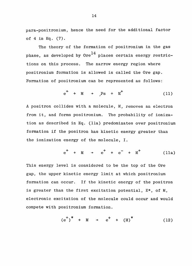
The theory of the formation of positronium in the gas 14 phase, as developed by Ore places certain energy restric-
tions on this process. The narrow energy region where
positronium formation is allowed is called the Ore gap.
Formation of positronium can be represented as follows:
+ e + M (11)
A positron collides with a molecule, M, removes an electron
from it, and forms positronium. The probability of ioniza-
tion as described in Eq. (lla) predominates over positronium
formation if the positron has kinetic energy greater than
the ionization energy of the molecule, I.
+ e + M + + e + e (lla)
This energy level is considered to be the top of the Ore
gap, the upper kinetic energy limit at which positronium
formation can occur. If the kinetic energy of the positron
is greater than the first excitation potential, E*, of M,
electronic excitation of the molecule could occur and would
compete with positronium formation.
+ + * e + (M) (12)

15
If the ionization potential oi Mis greater than the binding
energy of positronium, 6,8 eV, the reaction is endothermic.
Only positrons possessing enough kinetic energy, EKin > I -
6.8, can form positronium. This makes, I-6.8, the lower
positron energy threshold, T, for positronium formations.
The Ore theory is based on three basic assumptions:
(1) All positrons reach the top of the Ore
gap, I, without being annihilated.
(2) There is a statistical distribution of
positron energies in the range between
I and E = thermal.
(3) All positrons whose kinetic energy
lies within the Ore gap will form
positronium.
Figure 3a is an energy diagram showing the Ore gap in
gaseous argon and Figure 3b is a plot of the hypothetical
dependence of the positronium formation probability in
argon gas as a function of positron energy. 15 Green and
Lee note that the curve is meant to illustrate general
features only. The actual formation probability has been
measured by Gittleman 16 in a variety of gases and was
found to average about 30% of positrons emitted.
Since the binding energy of positronium is less than
the ionization potential of most molecules, a considerable
number of positrons exist with energies below the Ore gap.

T 6.8 eV
:>, ~ •rl rl ·rl ..0 ro ..0 0 H 1. 0 p..
s:: 0
·rl ~ c-;l E H 0 0.5 ~
E ;:l
·rl s:: 0 H ~ ·rl 0.0 U1 0 0 p..
16
20.0 eV
15.8 eV
11. 6 eV
.,9.0 eV
0.0 eV
( a)
I
E*
Threshold
Threshold
E* I
5 10 15 Posi tro·n Energy, eV
(b)
I
Figure 3. (a) Energy Diagram of the Ore Gap and (b) Hypothetical Positronium Formation Probability in Gaseous Argon. (from Ref. 15)
17
The Ore theory does not place any energy restriction on
positron complex formation and positrons may bind to mole-
cules at any energy. Positron complex formation above or
within the Ore gap causes inhibition of positronium forma-
tion. However, positron complexes are generally thought to
form in the energy region beneath the Ore gap due to the
lower positron energy and lack of competition with positron-
ium formation.
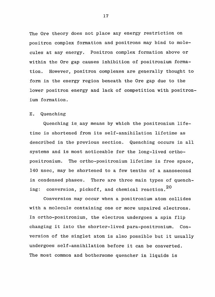
E. Quenching
Quenching is. any means by which the positronium life-
time is shortened from its self-annihilation lifetime as
described in the previous section. Quenching occurs in all
systems and is most noticeable for the long-lived ortho-
positronium. The ortho-positronium lifetime in free space,
140 nsec, may be shortened to a few tenths of a nanosecond
in condensed phases. There are three main types of quench-
. . . k ff d h . 1 t· 20 ing: conversion, pie o , an c emica reac ion.
Conversion may occur when a positronium atom collides
with a molecule containing one or more unpaired electrons.
In ortho-positronium, the electron undergoes a spin flip
changing it into the shorter-lived para-positronium. Con-
version of the singlet atom is also possible but it usually
undergoes self-annihilation before it can be converted.
The most common and bothersome quencher in liquids is

•
18
dissolved oxygen. Care must be taken to remove it from
the liquid in order to measure the positronium annihilation
rates. The mechanism by which oxygen quenches and the
procedure for degassing a liquid are discussed in detail in
the chapter on experimental methods. Other molecules that
are known to cause conversion quenching are NO, N02 , and
many of the paramagnetic transition metal cations and their
complexes.
Pickoff is the annihilation of the bound positron with
an electron of a colliding molecule. Again, pickoff is most
noticeable for ortho-positronium and occurs when the posi-
tron part of the positronium wave function sufficiently
overlaps with a singlet electron of the surrounding medium.
Hence the positron "picksoff" an electron from the molecule.
The ortho-positronium pickoff annihilation rate of 193
organic liquids has been measured by Grey, Sturm, and Cook. 21
They have found the average annihilation cross section,
<crv>, to correlate directly with the electron polarizability
of normal alkanes as calculated from their indicies of
refraction. Partial quenching cross sections were calcula-
ted for 27 structural functional groups (See Table I) and
can be used to predict molecular quenching cross sections.
The average error of the calculated cross sections for 151
compounds was 1.79%. The cross sections for the remaining
42 compounds could not be calculated because they contained

19
Table I. Average Quenching Cross Sections.
(From Re.t. 21)
CH3 CH2 CH C
C6Hll C6Hl0 C5H9 C6H5 C6H4 -CH=CH-CH2=CH-CH2=C(CH3)--CH=C(CH3)-H OH -0-CHO COOH C=O COO-F Cl Br NH2 P0 3:::
P04 :::
SH
Group <crv>,
Monosubstituted Cyclohexanes Disubstituted Cyclohexanes Monosubstituted Cyclopentanes Monosubstituted Benzenes Disubstituted Benzenes
Ethers Aldehydes Acids Ketones Esters
Phosphites Phosphates Thiols
-14 3 10 cm /sec
0.855 0.971 0.924 0.705 5.515 5.373 4.469 4.679 4.844 1.906 1.667 2.635 3.076 0.129 0.749 0.836 1.673 1.839 1.786 1.939 0.084 1.122 1.872 1.624 3.382 3.754 2.330

20
unusual structures such as. keto-enol forms or because the
ortho-positronium intensity, r2 , was so small that accurate
lifetime measurements could not be made.
The pickoff process in the condensed phase has been
characterized by Brandt 17 using a "free volume model" in
which the positronium atom is thought to occupy the inter-
stitial volume between the molecules. The pertinent
assumptions are:
(1) Mutual polarization of the lattice and
the positronium is neglected.
(2) The positronium is considered to be
thermalized.
(3) The lattice potential is rectangular
in-shape (Figure 4 gives a qualitative
description of this arrangement). The
potential well has height, U0 , radius,
r corresponding to an excluded volume 0
V0 and electron density, p0 ! A unit
cell has radius, r 1 > r 0 and cell volume
v1 . The free volume, V*, is equal to
Vl-VO.
The amount of free volume present in a liquid depends upon
the molecular properties of the liquid, the temperature,
and the pressure. Henderson and Millett 18 studied the
pressure dependence of the ortho-positronium lifetime, T 2 ,

2 '!'Ps
,'~
uo
l
2 '!'Ps
I,._ Free -::l~ l Volume I
f-
Lattice Potential
Excluded Volume
Unit Cell
2 '!'Ps
-~ ~ rl ~
-~ fr-ro-~
Figure 4. Lattice Potential as Described by the "Free Volume Model". (from Ref. 17)
2 '!'Ps
~ f-J

22
in 22 organic liquids and established that it decreased
linearly with decreasing specific volume, V(P)/V 0 , where
V is the volume at STP. Wilson, Johnson, and Stump 19 0
investigated both the temperature and pressure dependence
of T 2 in a series of liquids. They found the lifetimes to
follow
(13)
whereµ is a characteristic constant for each liquid. The
lifetimes of ortho-positronium in liquids that cannot be
described by these relationships will be discussed in
Chapter 3.
The validity of the "free volume model" is further
substantiated by two photon angular correlation experiments.
When singlet annihilation occurs, the two photons are
emitted in exactly opposite directions, 8 =~,if the
center of mass of the electron-positron pair is at rest.
However, the center of mass is in motion for all practical
situations and the angular distribution, C(8) versus a, of
the annihilating photons appears bell-shaped about a=~
radians. The angular distribution may be used to obtain the
momentum (p) distribution, C(p) versus p. 22 An example of
both the angular and momentum distributions is shown i~
Figure 5,
components.
Momentum distributions generally consist of two 23 It was pointed out by Ferrell, that para-

, , I. I 0
23
....... Low Momentum c3mponen t ~--High Momentum omponent
, , , I
~ , ; ,:
I •
f\ f ' I • ! \ ," --,,
' ' ' \ I \ r ' I I
I ' I \ I \ I \
' ' I \ I \ ' \ ' \ , \ , ' ,/' ,,
, '
,
e = 7T (a)
5 10 -3 Momentum (p), xlO me
(b)
15
Figure 5. (a) Angular and (b) Momentum Distributions of the Annihilating Photons.
24
positronium should give rise to a relatively low momentum
component since it usually decays by self-annihilation of
the electron-positron pair. Direct positron and ortho-
positronium pickoff annihilation occur with electrons bound
to molecules of the system. These photons should contribute
to a relatively higher momentum component because if the
positron or positronium is thermalized, as is required by
the bubble model, the primary contribution to the momentum
of the center of mass of the annihilating pair will come
from the high momentum bonding electrons. If this is true,
the intensity of the low momentum component should correlate
with the intensity of para-positronium as measured from
lifetime measurements. Kerr et a1 24 have compared the two
intensities for ten organic liquids. The two measurements,
taken from two completely different experiments, agreed
within experimental error for all 10 compounds.
The higher momentum component of the momentum distribu-
tion can be used as an experimental verification of calcula-
ted electron momentum distributions if pickoff annihilation
occurs as described by the "free volume model." The momen-
tum distributions for electrons in C-C and C-H bonds have
been calculated using analytic SCF functions for atomic
carbon orbitals and Heitler-London-type functions for the
two paired electrons in the C-C and C-H bonds. 25 The authors
then computed a theoretical electron momentum distribution

25
curve for hexane and decane. The results for decane are
shown in Figure 6, Component A is approximately gaussian
and corresponded to the low momentum part due to para-
positronium. Component Bis the calculated C-H contribution
and Component C is the calculated C-C contribution. When
fit to the experimental curve, the relative areas under
Components Band C were found to be in the exact ratio of
the electrons in the C-H bonds compared to the electrons
in the C-C bonds. For hexane and decane these ratios were
28/10 and 44/18 respectively. They concluded that during
pickoff annihilation, the positron of ortho-positronium
annihilates primarily with the bonding electrons of a mole-
cule.
The third kind of positronium quenching is by chemical
reaction. Tao and Green 26 have divided this category into
four types: (1) oxidation by electron transfer; (2) re-
duction; (3) compound formation; and (4) double decomposition.
This thesis deals primarily with the chemical reactions by
compound formation and for that reason, it will be discussed
in detail in Chapter 3.
Figure 7 summarizes the many interactions of positrons
d . t . . t 20 H. h . t 1 an pos1 ron1um in wa er. ig energy posi rons ose
energy rapidly while slowing down. If a collision takes
place while the positron is in the Ore gap, positronium
atoms are formed with excess kinetic energy. About one-

,..._ 0..
'--' u
6 ~ Decanc (ClOH22) 0 0 o Experimental Points Theoretical Curve: A+B+C
4 l 2
0 0
I I
I
A
/ /
/
I I
I /
I /
I / \ I \
/ \ •
.... 2
\
' ' ..,. - ' ' ~
" /
, B
.... -....
-.. - -
A ... C(p-Ps) B ... C(C-H) C ... C(C-C)
....
.....
..... C ------
4 6 -3 8 Momentum (p), xlO me
10
0 0
0
12
Figure 6. Computed and Experimental Momentum Distributions for Decane. (from Ref. 25)
t:v G)

keV Range
6. 8 eV ~
>, b.O H Cl) i:::
i:,::i
0.0 eV--..,,,
+ e Birth
--+ e Ps
0.73 0.27
-...
,I,
+ e
.
Ps formation 2y Pickoff 3y
i i t ,
:: p-Ps conver- o-Ps sion ~
Oxidation qf Ps
Ps compound formati
Reduction of Ps
1 J I,
--; + conver- Ps e Ps -compound p-Ps sion o-Ps compound . ·-.
Pickoff
Figure 7. Positron and Positronium Decay in Water. (from Ref. 20)
on
r:-., -.J

28
third of the positrons will do this, three-fourths of them
forming ortho-positronium and one-fourth forming para-
positronium. If paramagnetic species are present, conver-
sion quenching may occur. Pickoff annihilation is always
possible. If strong oxidants are present, positronium may
be oxidized back to a free positron. Reduction of positron-
ium would form Ps-, which has a binding energy of 0.3 eV,
however, this species has not been observed. 8 Positronium
compounds may form at any time during or after thermalization.
Free positrons may annihilate or form positron complexes and
then annihilate. The possibilities for interaction are
numerous, some are possible only for positrons or positron-
ium, others are analogous to the reactions of the hydrated
electron or hydrogen atom, two species to which positrons
and positronium are often compared.

EXPERIMENTAL METHODS
A. Introduction
Positron lifetime measurements are usually carried out
by using a delayed coincidence technique. 27 This method is
the most applicable one for measuring short (less than 10- 4s)
nuclear mean lives. It requires that a start pulse be pre-
sent which originates from a zero-time physical event. Also,
an end-time event pulse is necessary so that both pulses
can be fed into a coincidence circuit. A graph of coinci-
dence rate plotted as a function of time is the lifetime
spectrum and can be analyzed to give the lifetime of the
positrons in the system. Improvements on the basic experi-
mental arrangement were made by Bell and coworkers when they
introduced the fast-slow principle 28 and the time-to-pulse-
height-converter.29
A large majority of the data presented in this work was
obtained by measuring a positron lifetime spectrum under
varying conditions. These spectra were then used to measure
the lifetime of free positrons as well as the lifetimes of
both electron-positron bound states in solution. Positron
annihilation rates are defined as the reciprocal of these
positron lifetimes. These rates were used to evaluate
annihilation rate constants. The measurements of certain
rates as a function of temperature may be used to obtain
various thermodynamic quantities. Hence, kinetic as well
29

30
as thermodynamic information was obtained in order to
determine the mechanism by which one of the positron species,
ortho-positronium 1 reacted; this was a major objective of
the thesis.
B. Positron Sources
In the study of positronium chemistry, the most widely
used source of positrons is sodium-22 which has a half-life
of 2.60 years. It may be purchased from some of the major
radionuclide distributors either as carrier free 22NaCl, 22 NaHC03 , or as carrier solutions of these compounds. The
decay scheme 30 of 22Na is shown in Fig. 8. A majority of
the decays (90%) cause positron emission and leave the
daughter nuclei, neon-22 1 in a very short lived (T = 3psec)
excited state. Electron capture (EC) decay, in which no
positron is formed, occurs ten percent of the time. The
ground state of sodium-22 lies 2.840 MeV above the ground
state of neon-22 and 1.564 MeV above the first excited state
of neon-22. However, the maximum positron energy is only
0.544 MeV due to the energy requirements placed upon
positron decay as explained in Chapter 1. The transition
from the first excited state of neon-22 to its ground state
takes place in a time two to three orders of magnitude
faster than the average lifetime of a positron in condensed
matter. Consequently, the 1.276 MeV gamma-ray can be used
to initiate the zero-time start pulse required for coinci-

EC, 10%-+
S+ (JI , 90,o
---,-.J.r:~-.:_~:UP~S~e~c,/ - -1.27 .MeV S+ o/. + , 0. 05,o
Neon-22
2.60 yr
Sodium-22
2 2 m C e
I O. 544 MeV
Figure 8. Decay Scheme of Sodium-22. (from Ref. 30)
3
2
1
0 Energy, i'lle V
uJ I-'

32
dence studies, and the annihilation gamma rays used for the
end-time signal.
All of the data presented in this study were taken on
positrons annihilating in the liquid phase. The solid sup-
port for the positron source was a 1 mil thick aluminum
foil, 5 mm by 10 mm in size. A water solution containing
the sodium-22 was added dropwise to the foil and evaporated
at atmospheric pressure under an incandescent lamp. This
procedure was repeated until the foil contained the desired
activity. This rather arbitrary amount of activity depended
upon the specific activity of the sodium-22 solution, the
number of drops added and the counting efficiency of the
detector system. Ideally, one tried to place enough acti-
vity on the foil so that a spectrum containing at least
15,000 counts in the peak channel could be obtained every
six to eight hours. In working with most organic liquids,
the solubility of the sodium-22 compounds was small and
very little activity was lost from the foil during the
course of the experiment.
Activity losses due to the degassing procedure will be
discussed in the sample preparation and degassing section
of this chapter. Positron annihilation in the aluminum foil
and Pyrex glass sample tubes has been studied 31 and found
not to be a problem when using the abovementioned procedures.

33
c. Fast-Slow Delayed Coincidence Counting
A typical arrangement for a fast-slow coincidence
timing system is shown in ·Figure 9. A fraction of the gamma
photons emitted during the positron decay and annihilation
processes in the source are stopped by the two plastic
scintillators (phosphors). Each unit consists of a phos-
phor optically coupled to a photo-multiplier (PHOTO-MULT)
tube. The phosphors used were Nation 156 plastic scintilla-
tors, 1" by l". They have a fast decay constant in compari-
son to the positron lifetimes and also high light output.
The photomultiplier tubes were RCA 8575 mounted on Ortec 265
photomultiplier bases (PM BASE). They were used for their
high gain, fast rise time, and are low in the emission of
thermal electrons. The output signals from these detectors
are simultaneously fed into two coupled electronic circuits.
The circuits consist of a fast inner loop and a slow outer
loop. Each circuit has two sides, a start side and a stop
side.
The inner circuit was used to accurately determine the
time interval between the formation of the positron and its
subsequent decay. The output from the anode of the detector
is sent to an Ortec 417 fast discriminator (FAST DISC). The
units are operated at a biased voltage in order to reduce the
noise level in the circuit by setting a lower threshold limit
for accepting pulses from the photomultiplier tube. Both
fast discriminators send out fast timing pulses to an Ortec

DYNODE
P.M. BASE I I ANODE
~ FAST I DISC
PHOTO-MULT TUBE bziJ SOURCE * NATON 156 (l"x 111
)
PHOTO-MULT TUBE
~ ~ FAST I BASE
ANODE DISC. I
DY NODE I .£.. POWER
1.28 MeV GATE
:> :>I TIMING S.C.A.
I
I START~ I
iTOP T.P.H.C.
~ DELAY
I I
0.51 MeV GATE --
I
1 I
IAMV I TIMING r-----1
S.C.A.
Figure 9. Simple Fast-Slow Timing System.
I SLOW COINC.
a ... LINEAR
GATE c,J .i::,.
I MULTI-CHANNEL
I ANALYZER

35
437 time-to-pulse-height-converter (TPHC). This unit
converts the time difference between the start and stop
pulses into a proportional pulse height signal. Before
this pulse is allowed to pass into the multichannel analy-
zer (MCA), certain energy and coincidence conditions must
be met. An Ortec 425 variable delay unit is inserted into
the fast circuit to calibrate the channel width, time incre-
ment per channel, of the multichannel analyzer. The cali-
bration procedure and the importance of this quantity will
be discussed later.
The outer or slow loop takes its signals from the
dynodes of the photomultiplier tubes. These signals have
not been fully amplified in the detectors and therefore must
first be amplified and shaped by means of an Ortec 113
scintillation preamplifier (SCINT PREAMP) and then an Ortec
440 shaping amplifier (AMP). Both sides of the slow circuit
contain an Ortec 420 timing single channel analyzer (TIMING
SCA). On the start side, this unit is biased so that an
energy window is created that will only accept pulses that
correspond in energy to very nearly 1.276 MeV. This is the
energy of the de-excitation photon emitted during positron
decay. Pulses substantially larger or smaller than this are
rejected by the unit. The timing single channel analyzer in
the stop side of this circuit performs the very same function
for 0.511 MeV pulses, those from the annihilation process.
If both the start and stop pulses reach the Ortec 409 slow

36
coincidence (COINC) and linear gate unit (this time is
called the resolving time and is usually less than a µs)
within a short time interval, the slow coincidence unit
opens the linear gate and the signal from the time-to-pulse-
height converter is allowed to pass into the multichannel
analyzer. Overall, three different multichannel analyzers
were used in this study. They were a Nuclear Data 2200, a
Northern 600, and a Packard. They were all operated in a
pulse height analysis (PHA) mode. These units will accept
pulses of varying heights and sort them accordingly. These
data representing the lifetime distribution are stored in the
memory and can be read-out of the units in hard copy form
onto paper, paper tape, or magnetic tape. Once the lifetime
distribution data are taken out of the memory, it can then
be computer analyzed into its various lifetime components.
The positron lifetime measurement begins when the
starting detector accepts the zero-time pulse corresponding
to the emission of a position and continues until the end-
time pulse from the decay of that positron is received. The
lifetime of that positron is stored in memory and the coin-
cidence circuits are cleared in order to measure the life-
time of another positron, etc. This procedure is analogous
to having a large number of positrons at time t=o and
observing their lifetime distribution.

37
D, Positron Lifetime Spectra
The end result of the experiment described in the
previous section is a positron lifetime spectrum. A typical
spectrum is shown in Fig. 10. The ordinate of Fig. 10 gives
the logarithm of the number of two-gamma decays while the
abscissa is the time axis in nanosecond units. A point on
the curve, (log N(t), t), represents the number of positrons
that have lived for a certain time t and then decayed by
two-gamma emission. This two component exponential decay
spectrum is typical of positrons decaying in a condensed
phase, The steeper short-lived component, A1 , is attributed
to the decay of free positrons, those which have not formed
a bound state with an electron, and para-positronium, the
singlet bound state. The more shallow long-lived component,
A2 , is assigned to ortho-positronium. Even though this
species lives in solution as a triplet, its positron annihi-
lates with a singlet electron by two-gamma emission before
it reaches its expected lifetime.
In general, a multicomponent exponential decay spectrum
has the following form.
N(t) = N. exp (-A.t) 1 1
+ background
where the N. 's are the pre-exponential constants that weight 1
the individual components, and the Ai's are the annihilation
rates for the various modes of positron decay. A mean life,

10 5
10 4
,-, 10 3 .µ '-"
>-/:4C',J
10 2
10
1 0
I _/
I
D
I I
I I
I C
I I
+ Time zero
+ lq = T1
~ ~
R2 y(t) = Dexp(-A 1 t) + Cexp(-\ 2 t) + background
~ ~
+ A2 = T2
~ .:::::::,,.
background
50 100 150 Channel Number, 0.193 nsec/channel
Figure 10. Typical Positron Lifetime Spectrum.
w 00

39
T., is shown as the reciprocal of the ith annihilation rate. l.
These spectra can be computer resolved into their various
· .. 11 ·tt b C . 32 components using programs or1.g1.na y wri en y umm1.ng
or Tao 33 and then modified in this laboratory. The programs
were run on the IBM 360/155 computer located at the Virginia
Tech Computing Center. Briefly, the programs perform a
linear least squares analysis on each component present in
the spectrum starting with the longest lived one and then
constructs a calculated spectrum. The lifetime, annihilation
rate, and intensity of each component is output along with a
calculated fit parameter. This fit is a rather complicated
function of the standard deviation and values less than 2.00
are generally acceptable. In addition to the printer output
is a Calcomp plot of the experimental data and the calculated
spectrum which can be obtained by using the PAL program. 34
An example of the Calcomp plot is given by Fig. 11.
This is a plot of the base ten logarithm of the coinci-
dence rate versus time. The calculated fit is 1.05. The
calculated lifetime and intensity qf the two components are
Tl= 0.398 nsec, I 1 = 80.4% and T2 = 2.162 nsec, r 2 = 19.6%.
The PAL program requires that the calculation be started
beyond the curved top of the peak at a point where the first
component appears to decay linearly. This distortion at the
peak is caused by the finite resolving power of the instru-
ment and will be discussed later. The total area under the

40
cj
r-1 0 ITT rn
5l 6 o~ l
~as 69 ~
( S
l N n O
Jl :JO i
B
,--j k.
B . .....
(JJ
B . Ui
8~ .LJ
~Ci) ~ ::J z
B_J
--il.u rnz
z ([ I gu . t'l
B
...... ~
8 ~
E:8.
. ro .µ ro ~
(l) a ·r-i
.µ (l) 'H
•r-i H
(l) ..c .µ
'H 0
.µ 0 r-i 0. P
. a 0 C
) r-i c-: u r-1 cl C
) •r-i 0. :>. E
-4
. rl rl (l) H
::i M
·r-i ~

41
two components is normalized by the program to 100% so that
by reporting the intensity of either component, one auto-
matically sets the intensity of the other. No such relation-
ship can be applied to the annihilation rates, however A1
remains fairly constant at 2.5 ns-l in the liquid phase and,
therefore, will not be reported here. It is A2 , the anni-
hilation rate of ortho-positronium and its intensity, I 2 ,
that have been shown to be of interest chemically. 35 A
quantity that is used to evaluate the ability of any fast-
slow coincidence unit to resolve a multicomponent spectrum
is termed the resolution of such a unit. This parameter
has time units and is defined as the full-width-at-half-
maximum (FWHM) of a prompt spectrum. A prompt spectrum is
one in which the zero-time and end-time pulses are received
by the detectors simultaneously. Ideally, a single spike
should be seen in the lifetime spectrum corresponding to
time t=o. Experimentally, this can easily be done by placing
a cobalt-60 source between the two detectors. Cobalt-60
decays by negatron emission and emits a 1.173 and a 1.333
MeV gamma ray coincidently. If the two timing single
channel analyzers are set so that these two photons are used
to start and stop the timing measurement, a prompt spectrum
can be obtained. Due to the inadequate time resolution of
the instrument, the prompt spectrum appears broadened about
t=o as shown in Fig. 12. The resolution, FWHM, was typically
300-400 psec for the experiments reported here.

4
,,...._ U1 ..µ 3 s:: ;:l 0
C) ..._, b.O 0 ~
2
1 t = 0
Time, nsec
Full-Width-at-Half-Maximum
Figure 12. Prompt Spectrum of Cobalt-60.
~ ~

43
By inserting a known delay, i.e. 16 nsec, into the
timing circuit of Fig, 9, the prompt spectrum can be moved
16 nsec down the time axis. The number of channels between
the maximum of the prompt spectrum with no delay and the
maximum of the prompt spectrum with a 16 nsec delay can
then be used to calibrate the channel width, time increment
per channel. For this work, a 16 nsec delay caused the
prompt maximum to move 83 channels which represents a channel
width of 0.193 nsec/channel. This parameter is essential for
accurately evaluating the individual components (slopes) of
the lifetime spectrum and has been checked regularly.
E. Sample Preparation and Degassing
Measuring the positron lifetime distribution in the
liquid phase requires a sample vial capable of holding the
aluminum foil positron source and a few milliliters of
solution. The vial has been constructed so that its con-
tents could be easily degassed.
The rate constants for the reactions of ortho-positron-
ium were calculated by measuring the ortho-positronium
annihilation rates at various concentrations of the reactive
compounds. The sample tube used in this type of experiment
is shown in Fig. 13. It was constructed of cylindircal
Pyrex glass tubing, approximately 200 mm long, 10 mm i.d.
at the narrow counting end, and 25 mm i.d. at the top.

44
"0" Ring
Teflon Stopcock
Counting Region
Figure 13. Sample Tube used for Variable Concentration Experiments.

45
Perka1 31 has shown that a positron in a liquid such as
water will travel approximately 0.5 mm before annihilating.
A right angle side arm with Teflon stopcock was fitted to
the wider portion and a mole 10/40 ground glass joint was
attached so that the sample tube could be connected to the
vacuwn manifold. The lid was sealed to the main body of
the tube by a Teflon "0" ring and held by a clamp (not
shown). This arrangement has only been used for lifetime
measurements taken at room temperature.
For measuring annihilation rates at temperatures above
and below 295°K, a special sample tube was used. The
degassing bulb and sample tube for this type of measurement
are shown in Fig. 14. The sample tube was a Pyrex glass
tube about 100 mm long and 10 mm i. d. at the bottom. It
was tapered to a capillary and had a male 10/40 ground
glass joint on top. The wide bottom portion was broken so
that the aluminum foil positron source could be inserted
and then it was resealed. The solution to be counted,
about 2 ml, was introduced via a capillary syringe through
the top. The tube containing the source and solution was
then fitted into the female 10/20 joint of the degassing
bulb. The male joint of the sample tube protruded past the
end of the female joint of the bulb by approximately 8 mm
(see dotted line in Fig. 14). This prevented the solution
that splashed up into the bulb during degassing from becoming

46
Teflon Stopcock
Figure 14, Degassing Bulb and Sample Tube used for Variable Temperature Experiments.

47
contaminated by the stopcock grease and running back into
the sample tube. The degassing bulb was 75 mm in diameter,
contained a Teflon stopcock to isolate the sample from the
vacuum, and was fitted with male 10/40 ground glass joint
for attaching it to the vacuum manifold. This relatively
easy design proved quite adequate.
In dealing with organic liquids, the presence of
dissolved oxygen drastically reduces T 2 . This was first
shown by Lee and Celitans 36 in 1966 and later by Cooper et
a1 37 in 1967. Even today, data that was taken in the
presence of dissolved oxygen is still appearing in the
literature and must be discounted. The process responsible
for the shortening of the ortho-positronium lifetime has
been found to be conversion quenching. 38 Arguments are
made indicating that the triplet ortho-positronium reacts
with the unpaired electrons of the oxygen molecules in such
a way that the electron of the positronium atom is caused
to spin-flip creating the much shorter lived para-positron-
ium. In order to remove this quencher, each sample must be
thoroughly degassed by a simple freeze-thaw technique. The
sample tube is attached to the vacuum manifold and the
section containing the solution is frozen by liquid nitrogen
to avoid any evaporation losses. The Teflon stopcock is -4 opened and the vial is evacuated to 10 torr using an oil
diffusion pump. The stopcock is then closed and the frozen

48
sample is allowed to come to room temperature. This allows
the dissolved oxygen to equilibrate between the solution
and the partial vacuum above it. The sample is then re-
frozen, the stopcock opened and the oxygen above the frozen
sample is pumped off. This procedure should be repeated
5-7 times or until the solution no longer is seen to give
off bubbles upon thawing. For the variable concentration
studies, the sample tube requires no further preparation
and can be counted immediately after degassing. For the
variable temperature studies, the sample must still be
sealed at the capillary. So, after the last degassing,
the sample was refrozen, the stopcock opened, and the
capillary heated with a propane torch so that the capillary
collapsed under the reduced pressure and the sealed sample
tube removed from its ground glass joint.
Repeated degassing causes the aluminum foil backing to
become brittle. When this occurs, the activity can be
removed by dissolving the sodium-22 compound in water and
then discarding the foil. The recovered activity can be
reused. The degassing process also causes some activity
to be worn off of the source. This will appear as a slower
counting rate each time the source is used. It cannot be
avoided and more activity must be added to the source period-
ically.

49
The counting room temperature was maintained at 22°c
(295°K) and no special temperature regulation was used for
the variable concentration studies. Measurements below
room temperature were carried out in a Dewar flask fitted
with a cold finger as shown in Fig. 15. The sealed
cylindrical sample tube is fastened to a glass rod by a
piece of rubber tubing and the temperature is measured by
a Fisher low temperature thermometer. A variety of low
temperature liquid nitrogen 39 slush baths were used along
with isopropanol/dry ice (-75°C) and water/ice (4°C) baths.
The Dewar was filled with the coolant and the cold finger
placed between the two detectors for counting.
Temperatures above room temperature were maintained
by the thermostated oil bath shown in Fig. 16. The oil,
Fisher oil bath oil, was stirred by a magnetic stirring bar
and insulated by the Dewar flask. The sample tube, thermo-
meter, and platinum heating coil were submerged in the oil.
The heating coil current was controlled by two thermistors
and regulated by an external potentiometer. The apparatus
was capable of reaching 220 (±2) 0 c.
F. Solvents and Solutes
The solvents used in this study were benzene, toluene,
n-heptane, and n-pentanol. Benzene and toluene were both
Fisher Spectroanalyzed, the n-pentanol was Fisher Research
Grade, and then-heptane was Phillips Research Grade. All

50
Thermometer
,, ....
Counting Region
Figure 15. Experimental Arrangement used for Low Temperature Lifetime Measurements.

51
0 Temperature
Regulator
Heating Coil and Thermistors
Stirring Bar
Figure 16. Experimental Arrangement used for High Temperature Lifetime Measurements.

52
were used without further purification; however, molecular
sieve material was added to remove dissolved water.
The organic nitro compounds are all obtainable from
Aldrich Chemical Company and were of the highest purity
available. Most solids were recrystallized and most liquids
were distilled until their melting points or refractive
indicies agreed with handbook values.

CHEMICAL REACTIONS OF ORTHO-POSITRONIUM
A. Diamagnetic Quenchers
There are certain diamagnetic compounds that are able
to quench the lifetime of ortho-positronium to such an
extent that the long-lived component of the positron life-
time spectrum is absent. Among them are the nitroaromatics,
quinones, certain compounds that resemble maleic anhydride
in structure and composition and some nitriles. Goldan-
skii40,4l was the first to observe this behavior in dilute
solutions of nitrobenzene in benzene.
If the ortho-positronium lifetime is shortened so that
it becomes indistinguishable with the lifetimes of free
positrons and para-positronium, then the positron lifetime
spectrum appears as a rapidly decaying one-component
exponential decay curve. This is thought to be caused by
rapid chemical reaction of the ortho-positronium. The
ortho-positronium annihilation rate, the one that gives
rise to the shallow component in the spectrum, increased
to such an extent that the long-lived component was "pushed"
into the shorter-lived steep one. However, inhibition of
positronium formation will also cause the long-lived compon-
ent to be absent from the spectrum. If ortho-positronium is
not formed in any significant amount, I 2~o and the long-lived
component lldrop out" of the spectrum.
53

54
Xt is rather simple to determine whether inhibition of
positronium formation or rapid chemical reaction is taking
place. The lifetime spectrum is observed as a function of
increasing solute concentration in a suitable solvent. One
that will give both a long-lived second component, t 2 >2 nsec,
and a fairly high second component intensity, r2 > 20%.
(These values should serve only as general guidelines).
Positronium atoms that react while still possessing a con-
siderable amount of kinetic energy must do so very early in
their lifetimes and annihilations by this mode appear in
the short-lived component. If on the other hand, the
annihilation rate remains constant but r2 decreases from
the value in the pure solvent, r2°, to zero, inhibition of
ortho-positronium formation is occurring. Goldanskii 41
proposed the following mechanism for the reaction of ortho-
positronium with nitrobenzene and other rapidly reacting
compounds.
2y Ps + M ~ (1)
M + 2y
The positronium atom is thought to form a complex with
the reacting molecule, M, and either annihilate while in
the complex (lower path) or, since all diamagnetic quenchers
are known to be strong electron acceptors, annihilate as a
free-positron following a charge transfer mechanism (upper

55
path), TF ~ 0,45 nsec in condensed matter. Two arguments
can be made against the charge transfer mechanism.
Although all quenchers are known to be strong electron
acceptors, not all strong acceptors quench ortho-positronium,
i.e. benzonitrile, benzaldehyde, and napthalene. Charge
transfer is energetically possible in solution only if the
following inequality is satisfied.
-I+ A+ Q + S > 0 (2)
where I is the ionization potential of the donor, A is the
electron affinity of the acceptor, Q is the Coulomb inter-
action energy of the ions, and Sis the salvation energy
of the ions. 41 The ionization potential of positronium is
constant and all compounds with large electron affinities
should at least react to some extent with ortho-positronium.
It is also difficult to envision the electron transfer step
of the mechanism. The positronium atom does not have a
nucleus in the usual chemical sense. Its positron and elec-
tron are light particles and should be delocalized in the
PsM complex. Charge transfer in a complex of this nature
has no significance in terms of molecular orbital theory.
This does not exclude electron-transfer reactions of
positronium via some other mechanism and indeed this has 42 been observed.

56
The second order rate constant for the reaction of
ortho-positronium with Min Eq. (1) can be obtained as
follows: 49
-d[Ps]/dt = k[Ps][MJ
Dividing by [Ps] yields
-dln[Ps]/dt = k[M]
(3)
(4)
Since M~M >>Ps , the reaction will appear to be pseudo-o 0
first-order. The left-hand-side of Eq. (4) is defined to
be the rate of disappearance of positronium, AM. Therefore,
A = k[M] (5) M
The ortho-positronium annihilation rate in a pure liquid
such as benzene is A (=A ) and 2 Benzene
kBenzene = A2 /[Benzene] (6)
The annihilation rate in benzene was measured to be 0.33 -1 nsec , this corresponds to a rate constant for the reaction
of 2.96 x 10 7 M-1sec- 1 .
The annihilation rate for a solution is actually the
sum of two rates, As, the rate in the solvent, and AM' the
rate due to the solute, M. If the solute is present in
small concentration, i.e. millimolar, the following approxi-
t . l"d 43 ma ions are va 1 :
57
[Solvent]~ constant (7)
AS ~ constant
and
(8)
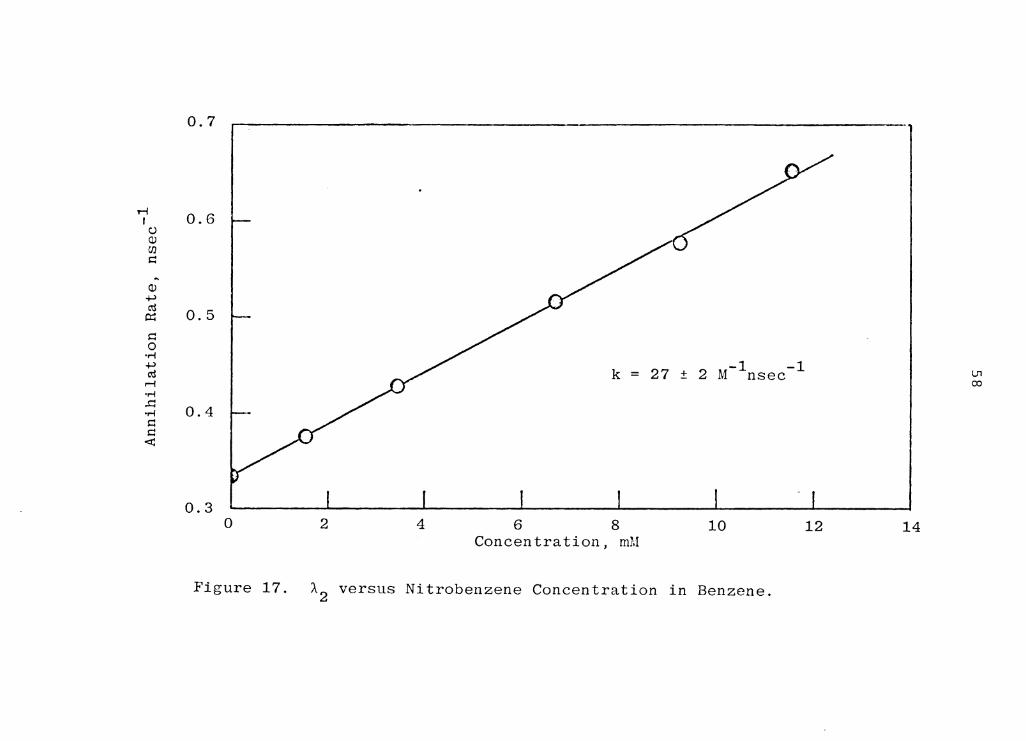
Any rate increase, A2-AS is due entirely to the solute. A
plot of A2 versus [M] has a slope that is equal to the rate
constant for the reaction between the ortho-positronium and
M. An example of one such plot is given in Fig. 17 for
nitrobenzene in benzene. The rate constant was found to -1 -1 be 27±2 M nsec , almost three orders of magnitude higher
than rate constant for the reaction with benzene.
The general statements made in this section apply to
all rapid reactions. For reasons of availability and
numerous possible substituents, the nitroaromatics were
chosen to be examined in this study. The following sections
will deal with the ortho-positronium reaction with them.
B. Conjugation Effects
Conjugation, or lack of it as the case may be, is a
major factor in determining the ability of a molecule to
chemically quench ortho-positronium. The microwave spectrum
of nitrobenzene shows that the molecule is planar 44 with an
internal barrier to rotation of 1000 ± 500 cm- 1 . When then
the nitro group is co-planar with the aromatic ring, it has
0.7
D
...; 0.6 I
t) (J) U1 0 s:: ~
(J) +,) ro 0.5 i:i:::
0
s:: 0
·r-i +,) I r/ -1 -1 ro k = 27 ± 2 M nsec I U1 r-i CX)
·r-i ..i:: 0.4 •r-i s:: s:: <X:
0.3 0 2 4 6 8 10 12 14
Concentration, mM
Figure 17. A2 versus Nitrobenzene Concentration in Benzene.

59
its maximum electron withdrawing effect and is best able
to remove electron density from the ring. 45
The steric interaction between the nitro group and the
methyl group(s) in the ortho positron was used to measure
the effect that conjugation losses had on the values of
the measured rate constants. Methyl groups were convenient
because their inductive and mesomeric effects are small.
Toluene, like benzene, reacts very slowly with positronium, 7 -1 -1 k ~ 10 M sec . The observed rate constants for some Tol.
model compounds are given in Fig. 18. Para- and meta-
nitrotoluene react slightly slower than nitrobenzene itself,
but the conjugation losses in the ortho isomer cause it to
react only one-third as fast. If a second methyl group is
placed adjacent to the nitro group, i.e. 2,6-dimethylnitro-
benzene, the nitro group is twisted to an even greater
extent out of the plane of the ring. It is therefore less
able to conjugate with the ring and its corresponding rate
constant drops further. This behavior was observed every
time a large group was placed next to the nitro group
(Appendix I lists all of the rate data taken in benzene
solution at 295°K).
Isolating the nitro group from the rr system was also
found to have a drastic effect on the measured rate constants.
In Figure 19, the rate constant for a-nitrotoluene is com-
pared to that of nitrobenzene and found to be drastically

o, +/o - -
o,+/o - 0~ /0 o, /0
N N N N
~ CH3 3HC CH3
,- ... ,,,..-~
0 0 / ' / ', , \ I \ I
I o+ I l o+ I \ I ' I ' , ,
'---' ,...__.,,,. CH3
CH3 -1. -1
k = 22 M nsec -1 -1 k = 21 M nsec -1 -1 k = 8.5 M nsec -1 -1 k = 0.39 M nsec
Figure 18. Steric Interactions that Force the Nitro Group out of the Plane of the Ring Cause a Reduction in the Rate Constant.
O'I 0

N0 2 I CH2
0 0-, + /
N
.. -.. 0 ,, ' I \
~ 0 + } ' / ... _ ....
-1 -1 k = 27 M nsec -1 -1 k = 0.15 M nsec
ro2 CH2 I R
R:
-H
-7 -1 -1 10 k, M sec
-CH 3
-CH 2CH3
3.47
4.55
5.17
Figure 19. Nitro Compounds in Which the Nitro Group is Not Attached
to a Conjugated System React Slowly with Ortho-Positronium.
O'I f-J

62
reduced. Similar small reaction rate constants are observed
for the nitroalkanes where there is no conjugation between
the nitro group and the alkyl group.
A third way of examining the effect of conjugation is
by measuring the rate constant for the reaction with certain
anhydrides that contain varying amounts of conjugation.
Fig. 20 shows a comparison of the observed positronium rate
constants for the reaction with succinic and maleic anhydride.
Succinic anhydride is unconjugated and exhibits a rate con-
stant indicative of pickoff quenching. Conversely, maleic
anhydride is highly conjugated and has resonance structures
that place a delocalized positive charge on all four carbon
atoms. The addition of the double bond caused the positron-
ium rate constant to increase by a factor greater than 200,
compared to succinic anhydride. These two are compared to
the highly conjugated chemical quencher, parabenzoquinone
which shows a much higher reaction rate constant.
C. Temperature Effects
If the mechanism given in Eq. (1) is correct, a study
of the temperature dependence of the rate constants should
provide information about the activation energy required to
form the various PsM complexes. The solvent was changed '
from benzene to toluene for these experiments because it
could be used over a much wider temperature range (200-
5000K).

le c\ 0- C C-0
-~0/-
-1 -1 k = 0.03 M nsec
-o_
HC CH
/ ,,.-- ..... \ I/ o+ '\ -
c c_o
~/ 0
-1 -1 k = 7.1 M nsec
Figure 20. Effect of Conjugation on Positronium Rate Constants.
0-
,---/ ... , I \ I o+ I ' I ' , __,,,
o-
-1 -1 k = 50 M nsec
°' w

64
First the temperature dependence of the solvent anni-
hilation rate had to be determined in order to use Eq. (8)
for calculating the rate constants. Fig. 21 shows a plot 0 of A2 (=~ 8 ) versus T( C) for toluene. A linear least squares
program was used to find the best fit to the data. It was
found that
-4 -1 A8 (T) = 0.3368 - (6.60 x 10 ) T nsec (9)
The second-order rate constant for toluene changed regularly 7 -1 -1 o 7 -1 -1 from 3.45 x 10 M sec at -75 C to 2.97 x 10 M sec
at 170°c.
When the annihilation rate of a 9.77 mM solution of
nitrobenzene in toluene was measured over this temperature
range, a rather interesting behavior was observed. The
observed rate constant, kb, when plotted against the 0 S
reciprocal Kelvin temperature, increased linearly from
-75°C up to approximately room temperature, 103;T°K = 3.4,
and then decreased linearly as the temperature was raised
further. 46 This is shown in Fig. 22. A comparison is made
in this figure between the temperature dependence of the
rate constants in toluene and the nitrobenzene solution.
The difference between the two rate constants is greatest
around room temperature. But at the high and low temperature
ends they begin to approach each other. Deviations from
typical Arrhenius behavior was found for other nitroaroma-
tics. Fig. 23 shows the log k versus 1/T curves for p-

,..-i I
c:.) 0) en s:: ~
0.40
0.35 A2 (T) = 0.3368 - (6.6xl0- 4 ) T
0) +> ro o:: 0. 30 s:: 0
·r-1 +> ro r--i ·r-1 ..c: •r-1 s:: s:: c::i:
0.25
0.20.~~~~--:::~~~-::1-~~~~.J..._~~~...L~~~--L~~~~l.___~~~~ -100 -60 -20 20 60 140 180 100
Temperature, 0 c
Figure 21. \ 2 versus T (°C) in Toluene.
O'I U1

10
,-... r/1 .0
~o 9 I / b.O 0
....::1
8
7
--a-i:: u o--:J ~ o----a--
2.0 3.0 1000/T(°K)
4.0 5.0
Figure 22. Arrhenius Plots for the Reaction of Ortho-Positronium With 9.77 mM Nitrobenzene in Toluene (0) and Pure Toluene (0).
I O'I O'I

(> 7.36 mM p-Dinitrobenzene 11 I- y ..---.~ ... 0 2.02 mM p-Nitrobenzonitrile
t:... 16.12 mM p-Nitroanisole a 13.22 mM p-Nitroaniline
,-,. en .0 0
10 I .!t:l /A v ~ ~ I O"I b.O -..J 0 ~
9
2.0 3.0 1000/T(°K)
•1. 0 5.0
Figure 23. Arrhenius Plots for the Reaction of Ortho-Positronium with Various Nitroaromatics in Toluene.

68
dinitrobenzene, p-benzonitrile, p-nitroanisole, and p-
nitroaniline. The Arrhenius portions of these five curves
(this refers to the section of the curve with negative
slope) all have approximately the same slope, while the
non-Arrhenius sections (positive slope) have different
slopes. p-Nitroaniline could not be run below 4°C due to
its insufficient solubility in toluene below this tempera-
ture.
There are a variety of reactions that can cause
deviation from the Arrhenius law. In principle, even the
simplest kinetic processes should show a temperature de-
pendence of the activation energy, 47 although it is rarely
observed due to limited experimental temperature ranges or
accuracy. Deviation from the Arrhenius law of a different
nature can be found for reactions involving, for example
equilibria, parallel, or consecutive processes. 48 This may
be caused by a changing reaction pathway, rate determining
step, or any process that causes the observed activation
energy to change with temperature. For the type of devia-
tion shown in Figures 22 and 23, where the measured activa-
tion energy actually becomes negative at high temperatures,
only a few of these reactions are possible.
The inversion in the log k versus 1/T plot eliminates
the possibility of a reaction involving a consecutive or
parallel pathway. Deviation in the Arrhenius plot could

69
occur by this method but both activation energies would
be positive.
Formation of an unreactive substance in the sample
might explain the observed behavior. The nitroaromatics
could possibly decompose at higher temperature giving rise
to a product that reacts more slowly. This possibility was
ruled out experimentally. The data was obtained by first
measuring the rate constant at room temperature followed by
kinetic runs at increasingly higher temperatures. After the
measurement was taken at the highest temperature, the sample
was rerun at room temperature to check against decomposition.
In all cases, the two room temperature values agreed within
experimental error. Reversible formation of an unreactive
species has not been ruled out by this procedure. For
example, the positronium could react with a solvent-solute
complex. Although nitroaromatics do form these complexes
in toluene, the results in other solvents discounted this
explanation. See the section on solvent effects in this
chapter.
The positronium atom is expected to tunnel readily due
to its low reduced mass. 49 However, the tunnel effect,
when observed, usually causes a log k versus 1/T plot to
curve rather than invert as in the present case. A tunnel-
ing calculation has been made for both a positron and
positronium atom incident on a potential barrier of varying
height and geometry. 50 The results indicate that the prob-

70
ability of tunneling is very high. To apply these results
to the present situation is impractical at the present time.
The shape of the barrier and the nature of the tunneling
particle are not known. Figure 24 is a plot of log of the
transmission coefficient versus particle energy for a
positronium atom tunneling through a parabolic, square wave,
and Eckart barrier, 1 R wide and 20 kcal/mole high. 49 The
initial results are encouraging and further work seems
warranted.
A mechanism that satisfactorily explains the observed
behavior is the following:
Ps + M PsM k
-- 2 ~) M + 2y (10)
ortho-Positronium combines with the nitroaromatic molecule
to form a PsM complex in a reversible step. This complex
is thought to be of a nature in which the positron and
electrons are completely delocalized. The electron and
positron enter into different molecular orbitals of the
complex. The complex can either go on to annihilate the
positron, k2 , or decompose into an ortho-positronium atom
and molecule, k_ 1 . Since the concentration of M remains
essentially constant throughout the experiment, the mechanism
can be simplified to

8 b.O
3
0.0
-0.l
-0.2
-0.3
-0.4
-0.5 0
Eckart
square wave
parabolic
2 4 6 8 10 12 14 16 Positronium Energy, kcal/mole
Figure 24. Log(Transmission Coefficient) versus Positronium Energy for Three Different Potential Barriers.
18
....J I-'

Ps
I
k ' 1
..... k -1
72
PsM M + 2y
for k 1 = k1 [M]. For this mechanism, one obtains the
following equations.
-d[Ps] /dt
d [2y ]/ dt · = k2[ PsM]
(11)
(12)
These differential equations can be solved exactly 51 , 52
for the time dependence of the concentration of Ps, PsM
and M (or 2y). The exact solutions are found to be func-
tions of three parameters, s1 , s2 and s3 .
=
=
(p-q)/2
(p+q)/2 (13)
where p = k 1 1 + k 1 + k2 and q = (p 2-4k 1 1 k2 ) 112 . s3 is
related to the total equilibrium solution, the time inde-
pendent terms. If s 1 << s2 , there is a simple time dependence
of [Psl [ PsM J and [ M J which involves only exp (- s1 t). after
a short induction period. This inequality can be met if
k_ 1 , k2 >> k 1 1 which is equivalent to invoking the steady-
state assumption for the PsM complex. Letting d[fsM]/dt = O,

73
and
Therefore, if the steady-state assumption is valid,
the observed rate constant for the disappearance of
positronium (or the formation of 2y) is k 1k2/(k_ 1+k2 ).
In relation to Figures 22 and 23, the low temperature
limiting line corresponds to a situation in which
k2 >> k_ 1 so that the reaction rate, r, becomes
r = k 1 IM] f Ps]
(14)
(15)
The high temperature limit corresponds to the situation in
which k_ 1 >> k2 and the reaction rate changes to
(16)
where kEQ = k 1/k_ 1 . The correct mechanism must predict
that both the low and high temperature rate expressions be
first order in M since this is observed experimentally.
The activation parameter obtained from the low tempera-
ture line represents the activation energy, E (1), of the a
associative step, k 1 . The high temperature line can be
(17)
used to measure the sum of two activation parameters, ~HEQ
for the equilibrium step and the activation energy, Ea(2)
for the annihilation step.

74
(18)
These are shown schematically in Figures 25 and 26.
A non-Arrhenius section is present in all the plots.
The activation energy, E (2), is always positive, therefore a the results indicate that the PsM complex is more stable
than the separated moieties. Chapter 4 deals primarily
with this topic. Representing the barrier to annihilation
as a thermodynamic barrier, as was done in Fig. 26, pre-
sented a problem that was never fully clarified.
The activation parameters for the reactions of the five
nitroaromatics with positronium are listed in Table II.
(The activation parameters for all reactions appear in
Section E of Appendix I).
Two points can be made concerning the data taken in
toluene. The activation energies for the first step were
all small, approximately 1.0 kcal/mole, and fairly constant
throughout. This is indicative of a fast reaction. It is
interesting to note that if the second substituent on the
nitrobenzene molecule was electron withdrawing, the ~S a (-26°C) was more unfavorable. The order being OCH3> H >CN
N02 . The change in entropy was calculated from the average
value of the activation energy, Ea(l), in toluene by using
the following equation:
(19)

'"' r:n ,.Q 0
~ ",..,/
b.O 0 H
I I r I r I
E (2) I a
75
-k obs
E (1) a
1000/T(°K)
Figure 25. Typical Arrhenius Plot for the Reaction of Ortho-Positronium with Nitroaromatics Showing the Thermodynamic Parameters.

76
Ps + M
2y
Reaction Coordinate
Figure 26. Potential Energy Surface for Ortho-Positronium Reacting with a Nitro-aromatic Molecule.

Table II. Thermodynamic Data for the Reactions of
o-Ps in Toluene
Low Temperature Limit High Temperature Limit
E (1), a tis ( -26°C) , a Comp OU_I1_d kcal/mole eu*
p-Nitroaniline --- ---2,6-Dimethylnitrobenzene --- ---p-Nitroanisole 0.9 ± 0.1 -10.2
Nitrobenzene 0.8 ± 0.1 -9.7
p-Nitrobenzonitrile 1.0 ± 0.1 -9.2
p-Dinitrobenzene 1.1 ± 0.1 -8.9
p-Benzoquinone 1.0 ± 0.1 -10.5
* Calculated using the average E (1) value. a
b.HEQ + Ea(2), kcal/mole
-1.1 ± 0.1
-2.7 ± 0.3
-3.6 ± 0.3
-4.5 ± 0.3
-6.0 ± 0.5
<-4. 0
-7.5 ± 0.5
-..J I -..J

78
The concept of entropy changes as applied to positronium
complexes has not been reported previously, In terms
of reorganizing the positronium atom and molecule into
a complex, the results would tend to indicate that the
complex would more readily proceed to the transition state
with molecules containing electron deficient substituents.
A qualitative analysis of the stability of the compl-
exes can be obtained from the high temperature region of
the graphs. ~HEQ + Ea(2) is always negative. This indi-
cates that Ea(2) is relatively small because even when
complex formation is least likely, ~HEQ is negative but
small, the sum of the two energies is still negative.
The ability of nitrobenzene to complex with positronium
is probably the reason that it is the only mono-substituted
benzene known to rapidly react with ortho-positronium. In
order to react, the main requirements appear to be: (1)
conjugation, (2) strong electron withdrawing substituents,
and (3) an ability of the molecule to form strong molecular
complexes. 53 It has been shown 41 , that compounds that form
very strong molecular complexes, such as 7,7,8,8-tetra-
cyanoquinodimethane (TCNQ) and tetracyanoethylene (TCNE),
react at least an order of magnitude faster than nitro-
benzene, which forms rather weak complexes.
It was initially thought that the inversion in the log
k versus 1/T plots was caused by a conjugation effect as

79
described in the previous section. As the temperature was
increased, the nitro group would begin to rotate out of the
plane of the ring, and the observed rate constant would
decrease due to a loss of conjugation. For this reason,
the annihilation rate for a p-benzoquinone was measured as
a function of temperature. The Arrhenius plot is given in
Figure 27. p-Benzoquinone is known to react faster than
nitrobenzene with positronium and it also readily forms
molecular complexes. If the inversion was caused by a
loss of conjugation, the effect should not be seen for p-
benzoquinone which does not have a functional group that
could rotate out of the plane of the ring. However, it
behaved in a similar manner to the nitroaromatics, E (1) = a 1.0 kcal/mole and ~HEQ + Ea(2) = -7.5 kcal/mole, and the
mechanism given in Eq. 10 was retained.
The log kb versus 1/T plot for 2,6-dimethylnitro-o s benzene is also shown in Figure 27. This compound showed
unusual behavior in that no Arrhenius portion of this curve
was found. Instead of inverting, the curve remains con-
stant over a so0 c range. Either the complex is so weakly
bound due to the large loss of conjugation caused by the
steric-interaction between the two methyl groups and the
nitro group that it decomposes rapidly o~ lower tempera-
ture data are needed to see the break.

80
11
10 A 13.15 mM p-Benzoquinone 0 206. mM 2,6-Dimethylnitrobenzene
- 0 Pure Benzonitrile en
Ci .0 Pure 2-Nitropropane 0 ~ v b.O 0 ...:I
9
8 <> ·O
2.5 1000/T(oK) 3.5 4.5 Figure 27. Arrhenius Plots for the Reaction of Ortho-Positron-
ium with p-Benzoquinone, 2,6-Dimothylnitrobenzene, Benzonitrile and 2-Nitropropane in Toluene.

81
It was mentioned previously that benzonitrile and 2-
nitropropane react very slowly with positroniuro at room
temperature. Their complexes might not be stable at room
temperature but data taken at other temperatures could
possibly show compound formation. Figure 27 clearly shows
no evidence for compound formation with these two compounds
in the temperature range studied.
D. Solvent Effects
Similar Arrhenius data were taken using n-heptane and
n-pentanol as the solvents. The temperature dependence of
the solvent annihilation rate was measured and can be found
in Section D of Appendix I. Only three nitroaromatic com-
pounds were used to study the effect of the solvent on
these reactions; nitrobenzene, p-nitroanisole, and p-dini-
trobenzene. The Arrhenius plots and thermodynamic data
appear in Figures 28 and 29 and in Table III respectively.
Similar trends were found in these solvents. Figure 30
shows a comparison of the Arrhenius plots for the reaction
of ortho-positronium with nitrobenzene in all three solvents.
Since an inversion was seen in the Arrhenius plot obtained
inn-heptane, the possibility of a solvent-solute species
being responsible for the rapid reaction was now eliminated.
Nitroaromatics are not known to form molecular complexes
with alkanes.

11
10
9
8
2.5
Figure 28.
82
3. !'5
A 19.55 mM Nitrobenzene O 1.81 mM p-Dinitrobenzen C 26.75 mM p-Nitroanisole
1000/T( 0 I{) 4.5
Arrhenius Plots for the Reaction of Ortho-Positronium with Nitrobenzene, p-Dinitrobenzene and p-Nitroanisole inn-Heptane.

83
11
10
9 0
8
O 9.77 mM Nitrobenzene 0 7.72 mM p-Dinitrobenzene A 12.84 mM p-Nitroanisole
2.5 3.5 1000/T(°K)
4.5
Figure 29. Arrhenius Plots for the Reaction of Ortho-Positronium with Nitrobenzene, p-Dinitrobenzene and'p-Nitroanisole in n-Pentanol.

Table III. Thermodynamic Data for the Reactions of
o-Ps inn-Heptane and n-Pentanol
Low Temperature Limit High Temperature Limit
Ea(l), b. S ( -26°C) , a b. ~Q + Ea ( 2 ), Compound kcal/mole eu* kcal/mole
Solvent: n-Heptane
p-Nitroanisole --- --- -2.9 ± 0.4
Nitrobenzene 1.3 ± 0.2 -8.1 -4.4 ± 0.4
p-Dinitrobenzene 1.0 ± 0.2 -7.1 -8.0 ± 1.0
Solvent: n-Pentanol
p-Nitroanisole 1.2 ± 0.1 -7.3 -1.3 ± 0.8
Nitrobenzene 1.3 ± 0.2 -6.2 -3.5 ± 0.6
p-Dinitrobenzene 1.8 ± 0.3 -5.5
* Calculated using the average E (1) value. . a
CX) ,i::,.

11
8
85
3.0 4.0 5.0 Figure 30. Arrhenius Plots for the Reaction of Ortho-
Positronium with Nitrobenzene in (C) Toluene, (0) n-Heptane and (A) n-Pentanol.

86
The point of inversion in the curves is determined
by the slopes of the two limiting lines and the pre-exponen-
tial factor, A, for each observed rate constant. These are
A1 for the low temperature limiting line and A1A2/A_ 1 for
the high temperature limiting line. According to absolute
rate theory, these factors contain two terms that could
possibly affect the point of inversion. The first is the
transmission coefficient, K, and the second is the entropy
change. The inversion point in the nitrobenzene curves of
Figure 30 can be used to determine the ability of each
solvent to assist in reaching the transition state before
forming the PsM complex. For nitrobenzene and the other
two compounds, this ability increased following the order
n-pentanol >toluene> n-heptane (20)
This is the order expected when neutral species combine to
form charged or polar complexes. 53 The more polar the
solvent, the more able it is to neutralize the charge
separation.
E. Correlations
Many correlations were attempted before the temperature
effect of Section C was discovered. 54- 56 Numerous rate
constants for substituted nitrobenzene compounds were
measured in benzene at 295°K. The log of the relative rate
constants (relative to nitrobenzene) was correlated to a

87
variety of molecular para.meters that included the energy
of th.e lowest unoccupied molecular orbital (LUMO), the net
~ charge density of the aromatic ring, free valence, radical
localization energy, etc. The results were moderately good
considering that the observed rate constants were for diff-
erent combinations of k1 , 1_1 and k2 .
The reactivity of these compounds toward positronium
atoms at room temperature was correlated by use of the
Hammett equation for electrophilic and nucleophilic attack. 57
Again, the observed rate constants could be k1 , k 1k2/(k_ 1+k2 ),
or kEQk2 depending on where the inversion point occured in
the Arrhenius plot. An example of this can be found in I
Figure 23. At room temperature, the observed rate constant
for p-nitroaniline is kEQk2 , for p-nitroanisole it is k 1k2/
(k_ 1+k2 ), and for p-dinitrobenzene it is k1 . However, it
was found that around -25°C, most measured rate constants
are k 1 . Figure 31 is a Hammett plot for nucleophilic attack 58
using only k 1 rate constants as measured in toluene at
-2s0 c. 59 These preliminary results are encouraging and
further work at this low temperature seems warranted.

,,...... (l) s:: (l) N s:: (l) ..0 0 H .µ ·r-l s:: ~ ......._
U1 ..0 0
~ v b.O 0 ...:l
0. 20 ·-
0.10 ) -Log(kobs/knitrobenzene -
0.0
-0.10
-0.1 0.0 0.1 -cr
Figure 31. Hammett Plot for the Reaction of Ortho-Positronium with Substituted Nitraromatics in Toluene at -26°C.
0.2
CX) CX)

POSITRON AND POSITRONIUM COMPLEXES60
A. Introduction
There is now a considerable amount of evidence avail-
able both from this work as well as lifetime and angular
correlation experiments to indicate the existence of stable
positron and positronium complexes with atoms, ions, and
molecules. 8 , 26 , 61 - 65 Theoretical calculations of the
stability of positron complexes with atoms and atomic ions,
and of the positron lifetimes in these complexes have gener-. 61 66-69 ally been rewarding. ' The most extensive theoretical
work in this area has been done by Schrader and co-workers:
a 1970 paper 70 provides a general non-relativistic self-
consistent-field theory of one-positron, many electron
systems and explains the approximations involved in most of
the earlier work; a more recent paper describes a variational
treatment of e+H- which incorporates interparticle coordinates
in the wavefunction. 69 The most accurate result of Navin,
Schrader, and Lebeda 69 indicates that e+H- is 0.794 eV more
stable than separated positronium and hydrogen atoms. This
means that the positron binding energy (positron affinity)
of the hydride ion is on the order of 6.8 eV. Earlier
calculations indicated positron affinities on the order of - . 61 67 2 eV for Cl and alkali atoms. '
This chapter is concerned with the existence of positron
complexes with relatively large organic compounds. For large
89

90
compounds, containing manr electrons, a variational treat-
ment similar to that for e+H- is presently intractable,
and it is necessary to retreat to some form of the self-
consistent-field theory. 70 We take the natural approach
of employing the Born-Oppenheimer separation and the Hartree-
Fock approximation. The former implies that we treat the
nuclei as fixed point charges, and the latter, that we
treat the positron on an equal basis with the electrons,
calculating only average Coulombic interactions between all
light particles. In general this approach should give
reasonable results. The necessary corrections for more
accurate calculations will arise from short-range interparti-
cle potentials, and should be amenable to treatment by an
extension of Sinanoglu's theory of purely electronic corre-
lation effects. 71 The positron-electron correlation effects
are expected to be extremely important in the prediction of
positron annihilation rates, so we have not tried to calcu-
late these; we are concerned here only with the stability
of the positron and positronium complexes.
We make use of the approximate all-valence-electron
self-consistent-field theory developed by Pople and co-
workers,72 the so-called CND0/2 approximation. We seek
positronic and electronic molecular orbitals and express
both as linear combinations of the same set of Slater-type
atomic orbitals. 72173 This has the advantage of providing
a oasis for estimating the necessary integrals over positron

91
coordinates without a great deal of computation. For all
electronic matrix elements, the CND0/2 approximations and
the parameterization suggested by Pople and Beveridge were
retained. The positronic matrix elements of the core
Hamiltonian were estimated by comparison with the corres-
ponding electronic integrals. The latter were approximately
decomposed into kinetic and potential energy parts using the
virial theorem. A sign change of the potential part pro-
vided the approximation for the one-center positron matrix
elements. For the two-center core matrix elements, these
considerations were combined with the Wolfsberg-Helmholtz
approximation 74 and the formulation given by Cusachs and
Cusachs. 75 All Coulomb integrals were evaluated using the
CND0/2 approximations, but accounting of course for the
positive charge of the positron. It is recognized that
these procedures only provide first approximations. In
particular, the virial theorem is not strictly applicable
to the electronic integrals involving Slater-type orbitals,
and the Slater-type orbitals provide improper cusp behavior
for the positron wavefunctions.
The calculations in this chapter deal primarily with
positron complexes with closed shell molecules. By making
use also of the lowest unoccupied electronic molecular
orbital, we obtain a first approximation for the binding
energies of positron complexes with molecular anions.

92
(These are alternatively referred to as positronium-
molecule complexes).
B. Hartree-Fock Theory
The total Hamiltonian, in atomic units, for a one-
positron 2n-electron system is given by
H = E hcore(-) + µ µ
r µ<v
g µv
+ h core(+) + E p gµp' (1)
µ
where (using atomic units)
hcore(-) = -'i/2 /2 E za /rµa µ µ a.
hcore(+) = -'i/2 /2 + E za /rpa p CJ.
-1 gµv = rµv
-1 gµp = :-rllP
The subscriptsµ and v are used to indicate electron
terms, p indicates positron terms, and a. refers to nuclei.
The superscripts(-) and(+) will be used with electron
and positron terms respectively for clarity. The core
Hamiltonian terms include the kinetic energies and Coulombic
interactions with all nuclei of the molecule. For a system
containing 2n electrons, and one positron, the wave function
is
t/J = t/J (p)[(2n)!]-l/2 p (2)
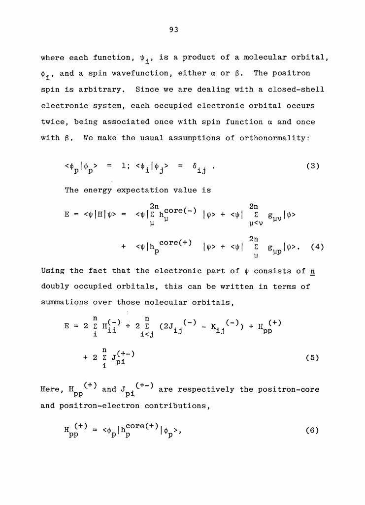
93
where each function, iµ., is a product of a molecular orbital, l.
~-, and a spin wavefunction, either a or S. The positron l.
spin is arbitrary. Since we are dealing with a closed-shell
electronic system, each occupied electronic orbital occurs
twice, being associated once with spin function a and once
with S. We make the usual assumptions of orthonormality:
<~ ,~ > = p p = 0 .. l.J
The energy expectation value is
E = <1/J IHI 1/J> =
+
2n 2n <1/JIE hcore(-) 11/J> + <1/JI E gµvli/J>
µ µ µ<v
<1/Jlh core(+) p
2n 11/J> + <1/JI r
µ g 11/J>. µp
(3)
(4)
Using the fact that the electronic part of 1jJ consists of n
doubly occupied orbitals, this can be written in terms of
summations over those molecular orbitals,
n (-) n (-) K .. <-)) (+) E = 2 E H .. + 2 E (2J .. + H i l. l. i<j l.J l. J pp
n (+-) + 2 E J . (5) i pl.
Here H (+) and J _(+-) are respectively the positron-core , PP Pl and positron-electron contributions,
(6)

94
J ~+-) ~ - <~ (p)$.(i)lr.- 1 I$ (p)$.(i)>, pi · f 1 1p p 1 (7)
' (-) (-) (-) and H1. 1. , J.. , and K.. are the purely electronic 1J 1J core interactions, Coulomb and exchange integrals involving
the molecular orbitals indicated by the subscripts. The
molecular orbitals are expanded as linear combinations of
the atomic valence-shell orbitals {xµ},
m m ,i,1· = E X C. 'I' µ µi µ
,1, = E X C 'l'p µ µp µ (8)
If we introduce charge-density and bond-order matrices for
both electrons and the positron,
n = 2 E
i p(+) =
µv (9)
the energy can be written in terms of integrals over atomic
orbitals:
E =
m - Cl/2)<xµ(l)xAC2)lri~lx 0 Cl)xv(2)>] + E
µ,v

95
Again, the first two terms are identical with those arising 72 in the simple closed shell electronic case, and the latter
two are caused by the positron,
H(+) = < (p)! hcore(+)I (p) > µv xµ P xv (11)
Minimizing the energy with respect to variations in the
electronic and positronic orbitals leads to two sets of
Hartree-Fock equations,
F e-) "' = 'I' i
(12)
where the electron and positron Fock operators are defined
as
and
hcore(-) + r (2 J.C-) J j
F(+) = hcore(+) + 2 r J.(+-) . j J
K.(-)) + J (+-) J p (13)
Jj and Kj are the usual electronic Coulomb and exchange
operators associated with the jth molecular orbital; J (+-) p is the positronic Coulomb operator,
J (+-)(r.) p -1 J <1>P* (r) [1/r. J </> (r) dT ; -p 1p p -p p
and J (+-) is the operator providing the Coulomb potential j
seen by a positron due to an electron in the jth orbital,

96
Jj(+-) 'r) = - / ~-* (r.) [1/r. J $. (r.) dTJ. •• ~p J -J. 1p J -1
For computational purposes, it is convenient to express
the energy as
E = (1/2) r p(-) (~-) + F(-)) µ,v µv· v µv
+ (1/2) E p~) ~v
(H(+) µv
+ F(+) µv ) , (14)
µ,v
where all matrix elements are in the basis set of atomic
orbitals. It should also be noted that in forming the
wavefunction (2) from the self-consistent solutions to
Eqs. (12) we consistently employ the Aufbau Principle.
That is, the 2n electrons are put into the~ lowest lying
electronic orbitals, and the positron is_ assumed to occupy
the positron orbital of lowest orbital energy, Ep.
C. Approximations and Parameterization
By using the zero-differential overlap approximation,
the multi-centered interaction integrals are simplified so
that
and the Fock matrix elements become
(15)

97
Fe_+) ::: H(+) - 1: p(-) Yµ~ µµ µµ A ~~
F(+) ::: H(+) (µ r v) llV llV
F(-) ::: H(-) - (1/2) p(-) Yµµ + 1: p(-) yµ). µµ µµ µµ A AA
- E pC+) y (16) A AA µ).
F(-) ::: H(-) - (1/2) pC-) Yµv (µ t- v) }1V µv µv
One of the CNDO approximations is to reduce Coulomb integrals
to one per atom pair, i.e., yµv = yAB' where Xµ is located
on atom A and x on atom B. " It should be noted that the electron Fock matrix con-
tains a
term is
contribution of the form, _p(-) y /2 and that this µv µv absent in the corresponding F(+). This exchange µv
term arises from the two-electron repulsions; since our
system contains only one positron, this term does not appear
in the positron matrix.
Eqs. (12) can now be solved by iterative techniques and
the electron and positron wave functions can be obtained in
which the electronic orbitals have been altered by the
presence of the positron, and the positron orbital has been
altered by the electrons.
The diagonal positron core matrix elements are approxi-
mated as
uC+) + µµ (x on atom A) µ (17)

98
u(+) is an atomic term containing the kinetic energy and µµ potential energy of the positron in the field of the Ath
core; the second term describes the positron interactions
with the other atomic cores.
The CND0/2 parameterization as described by Pople and
Beveridge 73 is used for all electron terms. However, for
the positron no data such as ionization potentials and
positron affinities are available. In order to parametrize
the positron Fock terms we relate them to the corresponding
electronic integrals as follows. For kinetic energy (T)
and potential energy (V) matrix elements,
T(+) = T(-) and v<+> (-) - - vµv µv µv µv (18)
so that
uC+) = T(+) + vC+) = TC-) v<-> µµ µµ µµ µµ µµ (19)
Applying the virial theorem,
TC-) Cl/2) vC-) (-) - - - - u µµ µµ µµ (20)
We see that
uC+) = - 3 uC-> µµ µµ
(21)
Treatment of the off-diagonal core terms is not as direct.
Because of the empirical nature of the bonding parameters, o(-) SAB , used by Pople and Beveridge, no direct conversion to

99
Bo(_+) was found. There.tore, we decided to combine the AB f u. 1 h ·1t . t· 74 "th th "d f Wol sberg-~e mo z approx1II1a ion wi e i eas o
Cusachs and Cusachs? 5 For the electronic core Hamiltonian
matrix, we have
=TC-)+ yC-) µv µv
~ S (2-IS l)CH(-) + H(-))/2 µv µv µµ vv
The analogous expressions for the positron are
= T(+) + yC+) µv µv
The terms in Eq. (23a) are now treated by the method of
Cusachs and Cusachs:
v<-t > ~ µv
S IS l(T(+) + T(+))/2 µv µv µµ vv '
s cv<+> + v<+>>12 µv µµ vv '
(22a)
(22b)
(22c)
(23a)
(23b)
and, substituting Eqs. (18) into the analogue of Eq. (19),
yields
(3/2) vC+) = llll

100
This gives directly
H(+) ~ (1/3) S (2 + IS I )(H(+) + H(+))/2 . µv µv · µv µµ vv (23c)
Values typically used 76 for the Wolfsberg-Helmholtz k(-) in
Eq, (22b) range from 1.75 to 2.0, and comparison with (22c)
shows that this corresponds to a range of lsµvl between 0
and 0.25. When these values are employed in Eq. (23c) and
the result equated to (23b), it appears that k(+) should be
in the range 2/3 to 3/4.
A computer program, PSCF, was developed by modifying
the CND0/2 program listed by Pople and Beveridge. 73 A
listing of the pertinent subroutines is given in Section E
of Appendix II. Along with the other approximations already
described, we employed Eq. (23b) for H(+) and varied k(+) µv over the indicated range.
D. Results
Using this formalism, we have studied the stability of
positron and positronium complexes of benzene and a number
of substituted benzene derivatives. In the process of
carrying out the iterations to self-consistency, two slight
problems arose. A number of calculations, especially with
the larger values of k(+), oscillated rather than converging
directly to an energy minimum. The oscillations were succ-
essfully eliminated by taking the modified density matrices
and averaging the new calculated matrices with the old ones

101
on each iteration, Also, for some of the symmetric mole-
cules, the symmetry was lost during the iteration process.
We believe that this resulted from round-off errors in the
positron density matrix, where the elements are generally
quite small. To eliminate the need for symmetry projection,
we restricted our solutions to the symmetric cases by
symmetrizing the molecular orbitals at each iteration.
The important results are listed in Tables IV and V
for the two limiting values of k(+) mentioned previously.
All calculations indicated that the positron should be
bound by these molecules. Two approximations for the posi-
tron binding energies are given: (-£ ) is the negative of p the positron orbital energy, and provides a Koopmans' theo-
rem77 estimate; the other entry (B.E.) was a direct calcula-
tion of the binding energy as the difference between the
total energy of the neutral molecule and that of the positron-
molecule complex. The two estimates are fairly comparable to
one another, but the former is always of greater magnitude
than the latter. The calculated positron binding energy
depends critically on the value used fork(+). This is
illustrated graphically in Fig. 32, which shows the two
estimates of the positron affinity of nitrobenzene as a
function of k(+). Corresponding to this, the number of
bound positronium orbitals also increased with k(+). For
the majority of the complexes, we found one or two bound
orbitals fork(+)= 2/3, and six to eight fork(+)= 3/4.

102
Table IV. Positron and Positronium Binding Energies,
a.u, (_C} k(_+) = 2,3
+ + e
Compound -e: B.E.(e) site(a) B .E. (Ps) p
Benzene 0,0082 0.0081 C-H -0.2197
Toluene 0.1877 0.1427 Alpha -0.0608 C-H
Fluorobenzene 0.2083 0.1030 Para -0.0809(b) C-H
Aniline 0.3375 0.2736 N-H +0.1184(b)
Benzonitrile 0.0780 0.0371 Meta -0.1726 C-H
Benzaldehyde 0.2256 0.1234 Carbonyl -0.0002 C-H
Nitrobenzene 0,0608 0.0200 Meta -0.1512 C-H
p-Banzoquinone 0.0213 0.0131 C-H -0.0232
(a) greater than 90% of thee+ charge density occurs here
(b) LUMO of the positronium complex is a cr orbital; in all other cases it is a TI orbital.
(c) 1 a.u. = 27.21 eV = 627.71 kcal/mole.

103
Table V, Positron and P.ositronium Binding Energies,
a.u, (C) k(+) = 3/4
+ e Compound + site(a) B.E. (Ps) -e: B.E.(e) p
Benzene +0.2840 +0.2831 C-H +0.0597
Toluene +0.4717 +0.4270 Alpha +0.2225 C-H
Fluorobenzene +0.4426 +0.3451 Para +0.1582(b) C-H
Aniline +0,6528 +0.5890 N-H +0.4339(b)
Benzonitrile +0.3671 +0.3194 C=N +0.1573
Benzaldehyde +0.4686 +0.3757 Carbonyl +0.2533 C-H
Nitrobenzene +0.4268 +0.3250 Para +0.1740 C-H
p-B enzoquinone +0.3137 +0.3084 C-H +0.2802
(a) greater than 90% of thee+ charge density occurs here
(b) LUMO of the positronium complex is a a orbital; in all cases it is a~ orbital.
(c) 1 a.u. = 27.21 eV = 627.71 kcal/mole.

. ::, . ti!
2 •
-1. 0 0.4
Figure 32.
104
0.6 k(+) 0.8 1. 0
Variation in the Po 9 itron Binding Energy in Nitrobenzene with kl+J. Koopman's Theorem Estimate (0) and Change in Energy Directly Calculated (A) for the Complex.
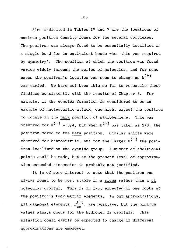
105
Also indicated in Tables IV and V are the locations of
maximum positron density tound for the several complexes.
The positron was always found to be essentially localized in
a single bond (or in equivalent bonds when this was required
by symmetry). The position at which the positron was found
varies widely through the series of molecules, and for some
cases the positron's location was seen to change ask(+)
was varied. We have not been able so far to reconcile these
findings consistently with the results of Chapter 3. For
example, if the complex formation is considered to be an
example of nucleophilic attack, one might expect the positron
to locate in the para position of nitrobenzene. This was
observed fork(+)= 3/4, but when k(+) was taken as 2/3, the
positron moved to the meta position. Similar shifts were
observed for benzonitrile, but for the larger k(+) the posi-
tron localized on the cyanide group. A number of additional
points could be made, but at the present level of approxima-
tion extended discussion is probably not justified.
It is of some interest to note that the positron was
always found to be most stable in a sigma rather than a pi
molecular orbital. This is in fact expected if one looks at
the positron's Fock matrix elements. In our approximations,
all diagonal elements, F(+), are positive, but the minimum µµ
values always occur for the hydrogen ls orbitals. This
situation could easily be expected to change if different
approximations are employed.
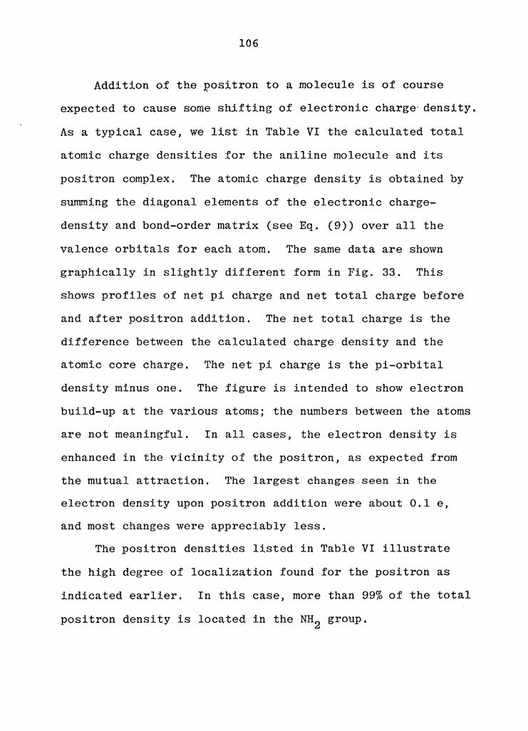
106
Addition of the positron to a molecule is of course
expected to cause some shifting of electronic charge· density.
As a typical case, we list in Table VI the calculated total
atomic charge densities for the aniline molecule and its
positron complex. The atomic charge density is obtained by
summing the diagonal elements of the electronic charge-
density and bond-order matrix (see Eq. (9)) over all the
valence orbitals for each atom. The same data are shown
graphically in slightly different form in Fig. 33. This
shows profiles of net pi charge and net total charge before
and after positron addition. The net total charge is the
difference between the calculated charge density and the
atomic core charge, The net pi charge is the pi-orbital
density minus one. The figure is intended to show electron
build-up at the various atoms; the numbers between the atoms
are not meaningful. In all cases, the electron density is
enhanced in the vicinity of the positron, as expected from
the mutual attraction. The largest changes seen in the
electron density upon positron addition were about 0.1 e,
and most changes were appreciably less.
The positron densities listed in Table VI illustrate
the high degree of localization found for the positron as
indicated earlier. In this case, more than 99% of the total
positron density is located in the NH2 group,

107
Table VI. Calculated Total Charge Densities for
Aniline and a Positron.-Aniline Complex
k(+) ;::: 3/4
Charge Density Charge Density in Complex Atom in Molecule Electron Positron
N 5.214 5.342 0.194
~ 0,939 1.041 0.399
CSUBST 3.770 3.789 0.002
CORTHO 4.010 3.971 0.001
HORTHO 1.057 1. 032 0.001
CMETA 3.912 3.897 0.000
HMETA 1.066 1. 014 0.000
CPARA 3.982 3.942 0.000
HPARA 1.064 1. 016 0.000

(l) 0.4 bll
0.2 ~ /'"
H . ' c'.i ./A, ..d / . u - . ~ r-i 0.0 c'.i I ---.µ ·--·-·---.--· 0 E-t -0.2 .µ
-o.4 L ~ (l) z
e H C C C C N-H
0.4
I ..... (l) 0 bll co H 0.2 cd' ..d u .,., 0.0 r -·- ·-·-. - -~--- ·-- ---.....__ ---·-. Pt .µ -0.2 (l) z
L IA -0.4
H C C C N-H
Figure 33. Profiles of Electronic Total Charge and Pi Charge for Aniline, Before C.~) and After(-·-) Positron Addition. The Position of the Highest Positron Density (not to scale) is Indicated in the N-H Bond.

109
It is possible to estimate positronium binding energies
for the -molecules considered. This is done by considering
the following cycle of processes, in which M denotes a neu-+ -tral molecule, and Ps indicates the positronium atom (e e ):
Ps + M -B.E, (PS) >
6.8 eV = 0.25 a.u. ~
+ e + e + M
PsM
1 I
+ E.A.(e M)
+ -e M + e
Thus, the positronium binding energy is approximately
+ + B.E. (Ps) = B.E. (e) + E.A.(e M) - 0.25 a.u. (24)
Here, B.E. (e+) is the molecular positron affinity discussed
earlier, E.A. (e+M) is the electron affinity of the positron-I
molecule complex, obtained by Koopmans theorem from the or-
bital energy of the first unoccupied electronic orbital in
the complex, and the last term is the dissociation energy of
the ground state of the hydrogen-like positronium atom. 80
The values obtained from Eq. (24) are listed in Tables IV
and V for each molecule.
These calculations do not unambiguously show whether
these molecules form stable positronium complexes. For all
but.aniline, the PsM complex was found to be unstable with

110
respect to dissociation to Ps + M when k(+) = 2/3. But
with k(+) = 3/4, all positronium-molecule complexes were
found to be stable.
Positronium complex formation in liquids is entirely
consistent with the "free volume model" that is used to
describe pickoff quenching and may be considered as a special
case of it. In the "free volume model," the positronium is
repelled by the lattice potential of the molecules of the
liquid and forced to remain in the free volume. The pickoff
annihilation rate is determined by the small amount of over-
lap between the wave functions of the positronium and the
molecules of the liquid. In the case of nitroaromatic li-
quids, a free volume exists, they have a density, viscosity
and surface tension that is similar to that of many non-
reactive liquids. However, if complex formation occurs, as
indicated by our present experimental and theoretical results,
the positronium atom is not repelled by the molecules of the
liquid but is incorporated into them. In this reversible
complex, the positron occupies a molecular orbitals and is
no longer associated with the electron oi the positronium
atom. The observed rapid annihilation rate in nitroaromatics
is caused by the enhanced electron density at the positron
while in the complex.
The calculations do not entirely agree with the experi-
mental results of the previous chapter that showed complex

111
formation for only two ot the compounds studied, nitro-
benzene and p-benzoquinone, Schrader is presently perform-81 ing similar calculations for positronium complexes and he
also finds them to be bound but not quite as strongly. Other
t · t 1 t ct· 78179 t h h h t f recen experimen a s u ~es sugges tat t e ea so
complexation are negative and on the order of a few kcal/
mole. This apparent discrepency could be caused by any
number of reasons. Inaccurate parameterization of the PSCF
program is one possibility. The calculations were only for
a 1:1 complex and in solution this is not necessarily the
case especially if one is to use the "free volume model."
More results are needed for gas phase reactions in order to
properly test our calculations.

CONCLUSIONS
A. Summary
The mechanism for the rapid chemical reaction of ortho-
positronium with a nitroaromatic molecule, M, in solution
was found to be
Ps + M PsM
The annihilation step is preceeded by reversible complex
formation. Only diamagnetic compounds that form strong
molecular complexes were found to react by this mechanism.
Nitroaromatics are known to be strong electron accept-
ing molecules and this is directly related to their ability
to form these complexes. Because of this, substituents on
the aromatic ring were found to affect the reactivity of
.these molecules toward the positronium atom. Nitroaromatics
with electron withdrawing groups attached to the aromatic
ring were found to form more stable complexes with positron-
ium than those that contained electron donating ones.
The complexing ability of these molecules was found to be
heavily dependent upon conjugation of the nitro group with
the aromatic ring, Steric interactions that force the nitro
group out of the plane of the ring caused the forward rate
constant, k1 , to be reduced.
112

113
A solvent effect was observed for this mechanism.
Polar solvents were more able to assist the reactants in
reaching the transition state associated with the complex
formation step as compared to non-polar ones.
The results of CNDO calculations regarding the stability
of positron and positronium complexes with large organic
molecules showed that these complexes should be stable.
However, complex formation was predicted for molecules in
which no complex formation was observed.
B. Future Possibilities
The results of angular correlation experiments using
the nitroaromatics could be used to determine the type(s) of
electrons that annihilate the positron. Experiments similar
to those mentioned for hexane and decane could be used to
locate the bond(s) that contain the annihilation electrons,
i.e., C-C, C-H, C-N, or N-0.
Many improvements can be made concerning the approxima-
tions used in the molecular orbital calculation. For example,
the basis set used to construct the positron molecular orbi-
tals was by no means complete. Atomic positron wave functions
could be calculated and used here. These would also serve
to better parameterize the calculations. These complexes
were found to be stable in the absence of any external for-
ces, Unlike the liquid phase, gas phase experiments should
provide more realistic conditions under which the results of

114
these calculations could be evaluated. Since positronium is
formed above thermal energy, excited positronium complexes
are also possible and configuration interaction (CI) calcu-
lations should be examined,

REFERENCES
1. Dirac, P.A. M., Proc. Carob, Phil. Soc., 26, 361 (1930).
2, Anderson, c. D., Phys. Rev., 41, 405 (1932); Phys. Rev., · 43, 491 (1933); Phys. Rev. , 44, 406 (1933).
3. Feynman, R. B., Phys. Rev., 76, 749 (1949).
4. Hamilton, J. H., Langer, L. M. and Smith, W. G., Phys. Rev. , 112, 2010 (1958).
5, Fermi, E., Z. Physik, 88, 161 (1934).
6. Lee, T. D, and Yang, C. N., Phys. Rev., 105, 1691 (1957).
7, Arya, A. P., Fundamentals of Nuclear Physics, Allyn and Bacon, Inc., Boston, 1966.
8. Goldanskii, V. I., Atomic Energy Rev., 6, 5 (1968).
9. Heitler, W. ,· The Quantum Theory of Radiation, Clarendon Press, Oxford, 1954.
10. Horstman, H., J. Inorg. Nucl. Chem., 27, 1191 (1965).
11. Ore, A. and Powell, J. L., Phys. Rev., 75, 1696 (1949).
12. Mohorovicic, s., Astron. Nachr., 253, 94 (1934).
13. Ruark, A. E., Phys. Rev., 68, 278 (1945).
14. Ore, A., Univ. Bergen Arbok Naturvitenskap. Rekke, 9, (1949).
15, Green, J. and Lee, J., Positronium Chemistry, Academic Press, New York, 1964.
16. Gittleman, B. and Deutch, M., Ann. Prog. Report, Lab. Nucl. Sci., M.I.T., p. 139 (1958).
17. Brandt, W., Berko, S., and Walker, W.W., Phys. Rev., . 120, 1289 (1960).
18, Henderson, G. A. and Millett, W. E., Bull. Am. Phys. Soc. , '!_, 120 ( 1962) .
19. Wilson, R. K., Johnson, P. 0. and Stump, R., Phys. Rev., 129, 2091 (1963).
115

116
20. Merrigan, J. A., Green, J, H. and Tao, S. J., in Physical Methods ot Chemistry, Weissberger, A. and Rossiter, B, W., Ed., Vol. 1 of Techniques in Chemistry, Wiley-Interscience, Inc., New York, 1970.
21. Grey, P. R., Cook, C. F. and Sturm, C. P., J. Chem. Phys., 48, 1145 (1968).
22. Stewart, A. J., Can. J, Phys., 35, 168 (1957).
23, Ferrell, R. A., Rev. Mod. Phys., 28, 308 (1956).
24, Kerr, D. P., Chuang, S. Y., and Hogg, B. G., Mol. Phys., 10, 13 (1965).
25. Chuang, S. Y. and Hogg, B. G., Can. J, Phys., 45, 3895 (1967); Nuovo Cimento, 58, 381 (1968).
26. Tao, S, J, and Green, J. H., J. Chem. Soc., A, 408 (1968).
27. Siegbahn, K., Alpha- Beta- Ganuna-Ray Spectroscopy, Vol. 2, North-Holland Publishing Co., Amsterdam, 1968.
28. Bell, R. E., Graham, R. L. and Petch, H. E., Can. J. Phys., 30, 35 (1952).
29. Green, R. E. and Bell, R. E., Nucl. Instr., 3, 127 (1958).
30. Lederer, C. M., Hollander, J.M. and Perlman, I., Table of Isotopes, 6th Ed., John Wiley & Sons, Inc., New York, 1967.
31. Perkal, M. B., Ph.D. Thesis, Massachusetts Institute of Technology, 1969.
32. Cumming, J. D., BNL Report No. 6470.
33, Tao, S. J,, IEEE Trans. Nucl. Sci., 175, (1968).
34, Program PAL is listed in Section F of Appendix II.
35. Ache, H.J., Angewandte Chemie, Int. Ed., 11, 180 (1972).
36. Lee, J, and Celitans, G. J,, J. Chem. Phys., 44, 2506 (1966).
37, Cooper, A. M., Laidlaw, G. J, and Hogg, C., J, Chem. Phys.,46, 2441 (1967).

117
38. Chaung, S, Y,. and Tao, .s. J., Appl. Phys., 3, 199 (1974),
39. Rondeau, R. E., J, Chem, and Eng, Data,· 11, 124 (1966).
40, Goldanskii, V, I'., Mogensen, O. E. and Shantarovech, U, P. , Phys. Lett. , · 32, 98 (1970) .
41. Goldanskii, V. r., Positron Annihilation Conference, Kingston, Canada, Sept. 1971.
42. Nicholas, J.B., Wild, R. E., Bartal, L. J. and Ache, H. J., J. Phys. Chem.,· 77, 178 (1973).
43. For compounds that require high (molar) concentrations to observe changes in A2 , a program SLOW RATE has been written and is listed in Section B of Appendix II.
44. Hog, J. H., Nygaard, L. and Sorensen, G. O., J. Mol. Struct., 7, 111 (1970).
45. Katritzky, A. R. and Topsom, R. D., Angewandte Chemie, Int. Ed., 9, 87 (1970).
46, Program ARRHENIUS was developed to calculate points on an Arrhenius plot from the observed annihilation rate. See Section C of Appendix II for a listing.
47. Cobble, J. W., J. Amer. Chem. Soc., 86, 5399 (1969).
48. Pignataro, S., Distefano, G. and Foffani, A., J. Amer. Chem. Soc., 92, 6425 (1970).
49, Caldin, E. F., Chem. Rev., 69, 135 (1969).
50. Madia, W. J., Nichols, A. L. and Lengsfield, B. H., unpublished results.
51, Frost, A. A. and Pearson, R.·G., Kinetics and Mechanisms, 2nd Ed., John Wiley & Sons, New York, 1961.
52, Pyun, C. W., J. Chem. Ed., 48, 194 (1970).
53, For references see e.g.: a) Briegleb, G., Elektronen-Donator-Acceptor Komplexe, Springer Verlag, Berlin 1961; b) Rose, J., Molecular Complexes, Pergamon Press, Ox-ford, 1967; c) Molec·uiar Complexes, Foster, R., Ed., Elek Science, London 1973; d) Mulliken, R. S. and Person, W. B., Molecu:1a·r Complexes, Wiley, New York, 1969.

118
54, Madia, W. J., Nichols, A. L. and Ache, H.J., J. Chem. Phys, , 60, 335 (_1974),
55. Madia, W. J., Nichols, A. L. and Ache, H, J., Ber. Bunsenges. Phyk. Chem., 78, 179 (1974).
56, Madia, w. J. ' Nichols, A. L. and Ache, H. J. ' Appl. Phys. , ~' 189 (1974).
57. Madia, w. J. ' Nichols, A. L. and Ache, H. J. ' J. Phys. Chem., 78, 1881 (1974).
58, Ehrenson, S., Brownlee, R. T. C. and Taft, R. W., Physical Organic Chemistry, Vol. 10, Strei twieser, A. and Taft, R. W., Ed., Wiley, New York, 1973.
59, A program, HAMMETT, was written to calculate cr values using the Hammett equation. A listing of this program may be found in Section D of Appendix II.
60, Madia, W. J., Schug, J.C., Nichols, A. L. and Ache, H. J. , J. Phys. Chem. , 78, 2682 ( 1974).
61. Simons, L., Phys. Rev., 90, 165 (1953).
62. Green, R. E. and Bell, R. E., Can. J. Phys., 35, 398 (1957).
63. Horstman, H.J., J. Inorg. Nucl. Chem., 27, 1191 (1965).
64. For general references see the following monographs and review article a) Green, J. and Lee, J., Positronium Chemistry, Academic Press, New York, 1964; b) McGervey, J. 0., in Positronium Annihilation, Stewart, A. T. and Roellig, L. O., Ed., Academic Press, New York, 1967.
65, Chuang, S. Y., Holt, H. W. and Hogg, B. G., J. Phys., 46, 2309 (1968).
66. Goldanskii, V. I., Ivanova, A. V. and Prokopyev, E. P., JETP, 47, 659 (1964); Ivanova, A. V. and Prokopyev, E. P., JETP, 48, 1155 (1965).
67. Huang, Din Van, JETP, 49, 630 (1965).
68, Lebeda, C. F. and Schrader, D. M., Phys. Rev., 178, 24 (1964).
69. Navin, P. B., Schrader, D. M. and Lebeda, C. F., Appl. Phys., 3, 159 (1974); Phys. Rev., A, 2248 (1974).

119
70, Schrader, D. M. 1 Phys. Rev. 1 1(4), 1070 (1970).
71. Sinanoglu, 0. 1 Proc. Natl. Acad. Sci. 1 47, 1217 (1961).
72. Pople, J, A. 1 Santry, D, P. and Segal, G. A., J. Chem. Phys,, 43, Sl29 (1965); Pople, J, A. and Segal, G. A., J, Chem~. Phys., 43, S136 (1965).
73. Pople, J, A. and Beveridge, D. L., Approximate Mole-cular Orbital Theory, McGraw Hill, New York, 1970.
74. Wolfsberg, M. and Helmholtz, L., J. Chem. Phys., 20, 837 (1952).
75. O.lsachs, L. C. and Cusacks, B. B., J. Phys. Chem., 71, 1060 (1967).
76. McGlynn, S, P., Vanquickinborne, L. G., Kinoshita, M., and Carroll, D. G., rn·troduction to Applied Quantum Chemistry, Holt, Rinehart and Winston, Inc., New York, 1972.
77. Koopmans, T., Physica, !, 104 (1933).
78. Goldanskii, V. I. and Shantarovich, V. P., Appl. Phys., ~' 335 (1974).
79. Tao, S. J., Kelly, T. M., Chuang, S. Y. and Wilkinfield, J.M., Appl. Phys., 3, 31 (1974).
80. Bethe, H. A. and Salpeter, E. E., Quantum Mechanics of One- and Two- Electron Atoms, Springer-Verlag, Berlin, 1951.
81, Schrader, D. M., private communication.
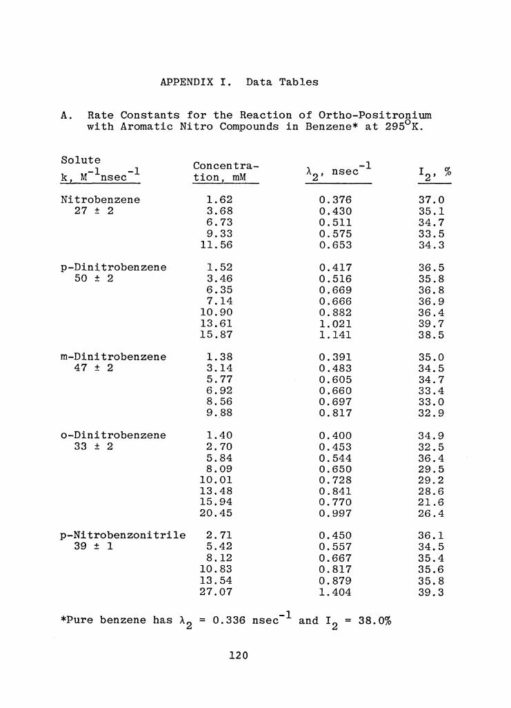
APPENDIX I. Data Tables
A. Rate Constants for the Reaction of Ortho-Positronium with Aromatic Nitro Compounds in Benzene* at 295°K.
Solute Concentra- -1 -1 -1 A2' I2, kz M nsec tion 1 mM nsec
Nitrobenzene 1.62 0.376 37.0 27 ± 2 3.68 0.430 35.1
6.73 0.511 34.7 9.33 0.575 33.5
11.56 0.653 34.3
p-Dinitrobenzene 1. 52 0.417 36.5 50 ± 2 3.46 0.516 35.8
6.35 0.669 36.8 7.14 0.666 36.9
10.90 0.882 36.4 13.61 1.021 39.7 15.87 1.141 38.5
m-Dinitrobenzene 1. 38 0.391 35.0 47 ± 2 3.14 0.483 34.5
5.77 0.605 34.7 6.92 0.660 33.4 8.56 0.697 33.0 9 .. 88 0.817 32.9
o-Dinitrobenzene 1.40 0.400 34.9 33 ± 2 2.70 0.453 32.5
5.84 0.544 36.4 8.09 0.650 29.5
10.01 0.728 29.2 13.48 0.841 28.6 15.94 0.770 21.6 20.45 0.997 26.4
p-Nitrobenzonitrile 2.71 0.450 36.1 39 ± 1 5.42 0.557 34.5
8.12 0.667 35.4 10.83 0.817 35.6 13.54 0.879 35.8 27.07 1.404 39.3
*Pure benzene has A2 = 0.336 nsec-l and r2 = 38.0%
120
%

121
Solute Concentra- -1 -1 -1 >i.2' !2, % k, M nsec tion, mM nsec
m-Nitrobenzonitrile 2.58 0.434 35.1 39 ± 2 5.16 0.521 34.3
7.74 0.636 33.5 10.32 0.704 33.5 12.91 0.830 35.6 15. 49 . 0.963 37.2
o-Nitrobenzonitrile 2.49 0.416 33.2 39 ± 2 4.97 0.476 29.7
7.46 0.627 31. 3 9.94 0.722 31. 8
12.43 0.794 31. 8 14.92 0.917 33.2
m-Nitrobenzotri- 1. 88 0.403 36.8 fluoride 3.76 0.475 36.4 38 ± 1 7.52 0.605 35.6
11.27 0.748 36.1 15.03 0.911 38.7 16.91 0.982 38.6
o-Nitrobenzotri- 3.14 0.409 34.6 fluoride 6.27 0.501 32.4 25 ± 1 9.41 0.582 31. 5
12.54 0.644 30.4 15.68 0.723 29.1 18.82 0.810 28.3
p-Nitrobenzaldehyde 2.50 0.434 36.5 40 ± 2 4.99 0.533 34.6
7.49 0.659 34.4 9.99 0.743 34.5
12.49 0.839 34.7 14.98 0.936 35.1
m-Nitrobenzaldehyde 2.42 0.424 35.9 35 ± 1 4.84 0.506 36.2
7.27 0.594 34.5 9.69 0.679 35.0
12.11 0.741 32.0 14.53 0.860 35.0

122
Solute Concentra- -1 -1 -1 A2' I2, % k, M nsec tion 2 mM nsec
o-Nitrobenzaldehyde 3.00 0.428 35.3 32 ± 2 6.00 0.513 32.2
9.00 0.614 31. 7 12.00 0.709 33.2 15.00 0.800 33.8 18.00 0.932 34.4
p-Nitroacetophenone 2.52 0.411 33.0 38 ± 2 5.05 0.533 32.6
7.57 0.626 31. 2 10.10 0.758 33.3 12.62 0.803 28. 6 15.14 0.906 28.7
m-Nitroacetophenone 2.32 0.401 35.9 30 ± 2 4,64 0.485 36.4
6.96 0.546 33.9 9.28 0.613 34.1
11.61 0.701 34.4 13.93 0.753 33.6
o-Nitroacetophenone 2.88 0.412 34.4 30 ± 2 5.76 0.504 32.1
8.64 0.599 31. 3 11. 52 0.649 30.1 14.40 0.736 27.8 17.27 0.873 31. 6
p-Nitrobenzoic acid 0.17 0.349 37.9 29 ± 5 0.33 0.356 36.9
0.50 0.357 37.2 0.66 0.364 36.8
m-Nitrobenzoic acid 4.35 0.481 35.9 28 ± 2 8.70 0.576 32.2
13.05 0.694 32.9 17.4 0.816 30.8 26.1 1.092 32.2
o-Nitrobenzoic acid 1.04 0.366 36.5 20 ± 2 2.60 0.399 34.5
3.64 0.415 32.6 5.20 0.428 33.0 7.79 o. 527 33.0
10.39 0.538 29.8

123
Solute Concentra- -1 -1 -1 ).2' !2' % k, M nsec tion, mM nsec
p-Nitrotoluene 5.89 0.465 38.1 22 ± 2 11.60 0.580 33.9
22.60 0.826 37.2 29.45 0.972 34.4
m-Nitrotoluene 1. 53 0.392 34.3 21 ± 2 5.62 0.487 35.0
9.20 0.581 35.3 16.95 0.743 35.1 22.50 0.917 36.6 33.75 1. 018 29.7
o-Nitrotoluene 2.23 0.358 34.3 8.5 ± 2 4.24 0.360 32.0
8.48 0.420 32.9 12.72 0.455 32.0 16.35 0.457 31.2 23.10 0.515 29.9
2,6-Dimethylnitro- 36.75 0.346 64.2 benzene 73.50 0.372 60.5 0.39 ± 0.05 98.00 0.370 34.0
110.25 0.370 33.1 147.00 0.393 32.1
p-Nitroanisole 2.63 0.383 35.2 13 ± 2 5.25 0.396 35.1
7.88 0.455 33.1 10.51 0.477 33.9 13.41 0.517 32.6 15.76 0.549 32.2
m-Nitroanisole 3.33 0.420 36.4 27 ± 2 6.65 0.521 36.8
9.98 0.580 34.7 13.31 0.686 35.8 16.63 0.762 35.6 19.96 0.883 36.7
o-Nitroanisole 6.15 0.374 34.7 49 ± 8 12.30 0.411 33.0
18.44 0.439 31.2 24.59 0.449 27.5 30.73 0.481 28.8 36.88 0.532 28.6

124
Solute Concentra- -1 -1 -1 A2' I2' % k, M nsec tion, mM nsec
p-Nitrophenol 1.47 0.351 37.0 13 ± 2 2.94 0.371 34.2
5,87 0.406 33.4 8.81 0.452 31.6
11. 74 0.468 32.3 14.68 0.528 30.8
m-Nitrophenol 2.88 0.409 35.4 26 ± 2 5.76 0.486 34.2
8.63 0.560 32.8 11.51 0.623 33.6 14.39 0.698 32.9 17.27 0.802 33.2
o-Nitrophenol 3.17 0.438 36.7 33 ± 2 6.33 0.532 35.5
9.62 0.635 36.1 12.66 0.768 37.2 15.83 0.876 37.0 18.99 0.954 36.4
p-Nitro-N,N- 2.41 0.381 35.9 dimethylaniline 4.81 0.425 36.2 18 ± 2 7.21 0.463 34.8
9.62 0.512 35.9 12.02 0.551 35.2 14.42 0.592 35.5
p-Nitroaniline 1. 78 o. 327 35.0 5.1 ± 0.6 2,62 0.355 36.3
3.71 0.349 35.1 4.58 0.369 35.1 6,55 o. 367 35.6 6.85 0.376 34.2 9.17 0.384 33.7
10.28 0.372 33.5 11.78 0.395 32.9 13.10 0.394 33.0 15.71 0.427 32.5 18.33 0.421 31. 5
m-Nitroaniline 1.62 0.362 36.9 19 ± 2 3.36 0.401 35.8
6.20 0.454 33.9 8.07 0.492 34.9 9.31 0.529 33.1
11. 52 0.557 34.1 13.44 0.586 33.3

Solute -1 -1 k, M nsec
o-Nitroaniline 10 ± 2
p-Nitrophenyl Acetate 26 ± 1
o-Nitrophenyl Acetate 23 ± 1
p-Nitrobenzyl alcohol 25 ± 1
m-Nitrobenzyl alcohol 24 ± 2
o-Nitrobenzyl alcohol 20 ± 2
125
Concentra-tion, mM
4.35 8.70
15.53 21.76 29.01 36.26 43.52
2.29 4.59 6.88 9.17
11.47 13.76
2.47 4.94 7.41 9.88
12.35 14.82
1.37 2.74 5.49 8.23
10.98 13.72
2.97 5.93 8.90
11. 87 14.84 17.80
2.99 5.99 8.98
11. 98 14.97 17.96
-1 A2 , nsec
0.374 0.415 0.476 0.521 0.630 0.643 0.789
0.394 0.459 0.515 0.569 0.626 0.698
0.388 0.442 0.497 0.558 0.619 0.680
0.372 0.409 0.469 0.531 0.600 0.687
0.432 0.497 0.542 0.633 0,681 0.780
0.401 0.447 0.507 0.576 0.638 0.684
35.6 34.2 33.2 32.0 31. 9 31.6 31.1
35.6 33.7 33.6 34.3 32.2 32. 4
35.5 33.4 32.2 33.0 32.7 30.8
37.0 35.2 33.3 33.7 32.3 33.0
35.6 34.7 33.2 33.3 31. 7 33.7
34.2 34.3 32.0 32.6 32. 9 31. 9
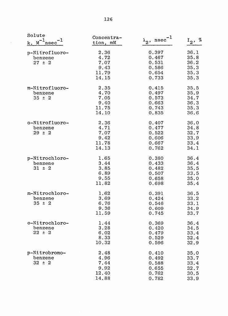
126
Solute Concentra- -1 k, -1 -1 tion 2 mM A2' nsec !2, % M nsec
p-Nitrofluoro- 2.36 0.397 36.1 benzene 4.72 0.467 35.8 27 ± 2 7.07 0.531 36.2
9.43 0.586 35.3 11. 79 0.654 35.3 14.15 0.733 35.3
rn-Nitrofluoro- 2.35 0.415 35,5 benzene 4.70 0.497 35.9 35 ± 2 7.05 0.573 34.7
9.40 0.663 36.3 11.75 0.743 35.3 14.10 0.835 36.6
o-Nitrofluoro- 2.36 0.407 36.0 benzene 4.71 0.477 34.8 29 ± 2 7.07 0.522 32.7
9.42 0.606 33.9 11. 78 0.667 33.4 14.13 0.762 34.1
p-Nitrochloro- 1.65 0.380 36.4 benzene 3.44 0.433 36.4 31 ± 2 3.85 0.482 35.5
6.89 0.507 33.5 9.55 0.658 35.0
11.82 0.698 35.4
m-Nitrochloro- 1. 62 0.391 36.5 benzene 3.69 0.424 33.2 35 ± 2 6.76 0.546 33.1
9.36 0.609 34.9 11. 59 0.745 33.7
o-Nitrochloro- 1.44 0.369 36.4 benzene 3.28 0.420 34.5 22 ± 2 6.02 0.479 33.4
8.33 0.529 32.4 10.32 0.596 32.9
p-Nitrobromo- 2.48 0.410 35.0 benzene 4.96 0.492 33.7 32 ± 2 7.44 0.588 33.4
9.92 0.655 32.7 12.40 0.762 30.5 14.88 0.782 33.9

127
Solute Concentra--1 -1 A.2' nsec I2' % k, M nsec tion, mM
m-Nitrobromo- 3.33 0.446 33.5 benzene 6.66 0.536 31. 9 36 ± 2 9.98 0.712 34.3
13.31 0.814 33.6 16.63 0.923 34.9 19.96 1.048 36.8
o-Nitrobromo- 1.48 0.374 34.1 benzene 2.95 0.418 33.2 22 ± 2 5.90 0.481 32.3
8.85 0.560 29.4 11. 80 0.583 30.5 14.75 0.680 31. 3
p-Nitroiodo- 2.05 0.418 35.8 benzene 4.10 0.476 34.6 32 ± 2 8.19 0.634 34.2
10.24 0.691 33.2 12.29 0.729 31. 4 14.34 0.796 32.0
m-Nitroiodo- 3.06 0.410 33.1 benzene 6.11 0.505 31.4 35 ± 2 9.17 0.587 30. 5
12.22 0.635 28.2 15.28 0.722 30.9 18.34 0.753 28.8
o-Nitroiodo- 2.79 0.443 34.8 benzene 5.58 0.519 33.0 23 ± 2 8.38 0.610 30.9
11.17 0.756 34.l 13.96 0.789 30.3 16.75 0.945 34.1

128
B. Rate Constants for the Reaction of Ortho-Positroniurn with Aliphatic Nitro Compounds in Benzene at 295°K.
Solute Concentra- -1 10- 7 k 2
-1 -1 tion 1 M ).2' nsec !2' % M sec
Nitromethane 1. 23 0.374 25.1 1.4 ± 0.3 2.47 0.383 19.2
3.70 0.407 16.5 4.96 0.426 14.8 6.27 0.462 13.6 8.64 0.464 12.1
Nitroethane 0.46 0.362 30.9 2.4 ± 0.3 0.93 0.364 27.1
1. 87 0.383 21. 7 2.80 0.420 18.8 3.73 0.447 16.9 4.67 0.451 14.8 6.53 0.500 12.7 8.40 0.510 12. 0
1-Nitropropane 0.38 0.355 28.2 2.0 ± 0.3 1. 50 0.363 21.4
2.25 0.387 20.4 3.00 0.398 17.2 4.50 0.435 15.7 5.25 0.454 14.1 6.00 0.473 13.4
2-Nitropropane 0.14 0.343 36.4 1.85 ± 0.2 0.37 0.345 32.5
1.11 0.358 24.9 2.22 0.376 18.7 4.45 0.430 15.1 6,68 0.464 12.4 8.91 0.499 10.9
11.14 0.551 9.5
a-Nitrotoluene 0.85 0.432 19.0 0.11 ± 0.02 1. 70 0.516 15.7
2.55 0.619 13.6 3.40 0.741 15.0 8.46 1. 235 10.3

129
C. Temperature Dependence of the Observed Rate Constants for the Reaction of Ortho-Positronium with Substituted Nitrobenzenes.
Solvent: Toluene
11.2' !2' % -1 -1 Solute T, 0 c -1
kl nsec M nsec
9.77 mM -75 0.433 27.3 5.1 Nitrobenzene -27 0.497 29.9 14.6
5 0.567 32.7 23.9 21 0.575 33.3 25.8 23 0.594 32.2 27.9 33 0.579 31. 5 27.1 38 0.576 33.8 27.0 42 0.597 34.6 29.6 56 0,531 34.2 23.7 58 0.511 34.5 21. 8 75 0,436 36.2 15.3 77 0.434 35.3 15.1 93 0.340 37.2 6.6
100 0.310 36.9 4.0 113 0.292 37.3 3.1 122 0.277 37.6 2.2 129 0.270 38.4 1.9 142 0.257 38.5 1. 5 154 0.244 39.4 1. 0
7.36 mM -75 0.430 33.3 6.0 p-Dinitrobenzene -45 0.459 32.4 12.7
-26 0.507 32.4 20.8 5 0.595 32.4 35.6
21 0.700 34.9 51. 3 35 0.752 35.3 59.5 54 0.819 35.0 70.4 70 0.927 36.5 86.5 85 1.043 40.0 103.6
105 1.125 40.9 116.5 123 1.262 46.0 136.7 149 1.231 46.5 134.8 163 1.046 46.8 111. 0 173 0,856 44.4 86.1

130
oc "2' -1 !2' % -1 -1 Solute T, nsec k, M nsec
2.02 mM -75 0.396 35.4 5.2 p-Nitrobenzo- 6 0.400 34.2 33.5
nitrile 21 0.402 34.4 39.5 40 0.418 34.5 53.4 56 0.428 33.8 63.8 71 0.447 35.8 77.8 87 0.441 34.9 80.2 95 0.434 36.2 79.5
102 0.441 36.6 85.0 117 0.437 36.8 88.2 132 0.397 38.1 72.9 152 0.350 40.0 56.5 176 0.267 41.1 23.0
16.12 mM -75 0.444 27.1 3.9 p-Nitroanisole -45 0.510 28.9 8.9
-26 0.530 30.2 11. 0 6 0.538 31.1 12.8
23 0.466 36.6 9.0 38 0.416 33.0 6.5 54 0.353 35.1 3.3 71 0.318 37.2 1. 8 86 0.296 36.3 1. 0
107 0.282 37.0 1. 0 130 0.262 38.6 0.7 146 0.254 38.9 0.8 173 0.235 40.3 0.8
13.22 mM 5 0.385 28.6 3.9 p-Nitroaniline 5 0.376 30.1 3.2
21 0.359 32.2 2.8 38 0.337 34.1 2.0 59 0.319 36.0 1. 6 77 0.304 37.6 1. 4 96 0.295 38.2 1. 7
111 0.277 37.4 1. 0 128 0.268 38.7 1.2 145 0.254 38.8 1. 0 160 0.242 39.2 0.2

131
A2' -1 I2' % -1 -1 Solute Tz oc nsec kz M nsec
206. mM -75 0.601 11. 8 1.04 2,6-Dimethyl- -40 0.587 14.3 1.10
nitrobenzene -27 0.550 17.4 0.95 5 0.419 27.8 0.42
21 0.364 31.1 0.20 37 0.342 32.8 0.15 56 0.324 35.0 0.12 74 0.307 35.7 0.09 91 0.284 35.8 0.04
106 0.277 36.8 0.05 117 0.273 35.8 0.07 130 0.261 36.5 0.05 142 0.261 36.7 0.09
Miscellaneous
13.15 mM -75 0.435 33.3 3.7 p-Benzoquinone 5 0.725 33.7 29.8
23 0.846 37.3 39.9 41 1.035 43.1 55.2 58 1. 014 38.7 54.4 78 1.193 48.5 69.0
1. 315 mM -75 0.390 38.9 2.8 p-Benzoquinone 5 0.367 36.4 25.8
22 0.372 37.1 37.6 46 0.373 37.7 51. 2 62 0.369 37.3 56.0 82 0.369 38.3 66.2
100 0.383 38.8 85.7 123 0.382 42.4 96.6 142 0.397 42.6 117.7 157 0.374 43.1 107.2 174 0.337 43.3 87.8 192 0.263 47.1 40.4
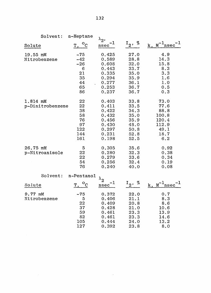
132
Solvent: n-Heptane A2,
-1 I2' % -1 -1 Solute T, oc nsec k, M nsec
19.55 mM -75 0.425 27.0 4.9 Nitrobenzene -42 0.589 28.8 14.3
-26 0.608 32.0 15.8 6 0.443 33.7 8.3
21 0.335 35.0 3.3 35 0.294 35.9 1.6 44 0.277 36.1 1. 0 65 0.253 36.7 0.5 86 0.237 36.7 0.3
1.814 rnM 22 0.403 33.8 73.0 p-Dinitrobenzene 22 0.411 33.5 77.6
38 0.422 34.3 88.8 58 0.432 35.0 100.8 76 0.456 35.9 120.4 97 0.430 48.0 112.9
122 0.297 50.8 49.1 144 0.231 52.8 18.7 161 0.198 52.5 6.2
26. 75 mM 5 0.305 35.6 0.92 p-Nitroanisole 22 0.280 32.3 0.38
22 0.279 33.6 0.34 54 0.256 32.4 0.19 76 0.240 40.0 0.08
Solvent: n-Pentanol ).2
oc -1 I2, % -1 -1 Solute T, nsec k, M nsec
9.77 rnM -75 0.372 22.0 0.7 Nitrobenzene 5 0.406 21.1 8.3
22 0.409 20.8 8.6 37 0.428 21. 0 10.6 59 0.461 23.3 13.9 82 0.461 23.3 14.6
105 0.444 24.0 13.2 127 0.392 23.8 8.0

133
A2' -1 I2' % -1 -1 Solute Tt oc nsec k, M nsec
7.72 mM -75 0.374 22.0 1.0 p-Dinitrobenzene 5 0.414 19.9 11. 6
22 0.462 19.6 17.8 40 0.516 20.6 24.9 65 0.657 24.2 43.1 88 0.758 27.3 56,9
113 0.924 34.3 99.2
12.84 mM -75 0.371 37.2 0.5 p-Nitroanisole 4 0.373 25.4 3.8
22 0.379 21. 0 4.3 39 0.385 21. 0 4.7 59 0.378 21. 5 4.1 81 0.377 22.3 4.6
101 0.359 23.4 3.4

134
D. Temperature Dependence of the Observed Rate Constants for the Reaction Ortho-Positronium with Solvents and Weakly Reactive Compounds.
).2' l0- 7k ' oc -1 I2, % -1 -1 Compound T, nsec M sec
n-Heptane -75 0.319 31. 6 3.90 -75 0.325 30.4 3.98 -45 0.323 32.0 4.20 -23 0.300 32.4 4.06
6 0.286 34.8 4.09 21 0.269 35.8 3.94 21 0.263 36.1 3.86 49 0.255 36.9 3.91 65 0.248 37.8 3.91 78 0.243 39.3 3.90 92 0.224 39.1 3.68
110 0.219 41. 7 3.70 131 0.208 41. 5 3.61 148 0.192 42.5 3.42 162 0.184 42.9 3.34 179 0.173 44.6 3. 23
Toluene -75 0.384 38.5 3.45 -75 0.381 37.3 3.42 -57 0.373 36.4 3.44 -27 0.355 36.4 3.46
3 0.333 37.3 3.43 3 0.337 33.8 3.47
21 0.319 36.8 3.39 37 0.312 36.5 3.40 53 0.303 36.2 3.38 72 0.294 37.1 3.39 91 0.277 37.8 3. 28
110 0.260 38.1 3.17 136 0.250 40.5 3.17 170 0.223 41.1 2.97
n-Pentanol -75 0.366 23.6 3.97 22 0.324 22.2 3.51 22 0.326 22.8 3.53 36 0.326 22.7 3.53 65 0.325 22.9 3.52 88 0.319 22.8 3.46
108 0.315 23.1 3.42

135
).2' l0- 7k , Compound T, oc -1 I2, % -1 -1 nsec M sec
Benzonitrile 5 0.541 12.4 5.52 23 0.458 10.5 4.67 40 0.428 9.7 4.36 67 0.457 12.2 4.66 86 0.435 12.1 4.44
112 0.443 14.0 4.52 135 0.379 12.6 3.87 157 0.379 13.8 3.86
2-Nitropropane 22 0.452 6.5 4.06 41 0.481 8.1 4.31 62 0.429 6.0 3.85 91 0.447 9.0 4.01
120 0.467 11. 3 4.18

E. Thermodynamic Data for the Reactions of o-Ps
Compound
Solvent: Toluene
p-Nitroaniline 2,6-Dimethylnitrobenzene p-Nitroanisole Nitrobenzene p-Nitrobenzonitrile p-Dinitrobenzene p-Benzoquinone
Solvent: n-Heptane
p-Nitroanisole Nitrobenzene p-Dinitrobenzene
Solvent: n-Pentanol
p-Nitroanisole Nitrobenzene p-Dinitrobenzene
Low Temperature Limit E (1), L\S (-26°C), a a
kcal/mole eu*
0.9 ± 0.1 0.8 ± 0.1 1.0 ± 0.1 1.1 ± 0.1 1.0 ± 0.1
1.3 ± 0.3 1.0 ± 0.2
1.2 ± 0.1 1.3 ± 0.2 1.8 ± 0.3
-10.2 -9.7 -9.2 -8.9
-10.5
-8.1 -7.1
-7.3 -6.2 -5.5
* Calculated using the average Ea(l) value.
High Temperature Limit
~HEQ + Ea ( 2 ) , kcal/mole
-1.1 ± 0.1 -2.7 ± 0.3 -3.6 ± 0.3 -4.5 ± 0.3 -6.0 ± 0.5
<-4.0 -7.5 ± 0.5
-2.9 ± 0.4 -4.4 ± 0.4 -8.0 ± 1.0
-1.3 ± 0.8 -3.5 ± 0.6
I I-' w m

APPENDIX II. Computer Programs
A, Introduction
Many trivial but time consuming calculations were
performed by the three convenience programs (SLOW RATE,
ARRHENIUS, AND HAMMETT) listed in this appendix. They are
written in either FORTRAN (IV) or WATFIV for use on an
autobatcher.
Section E contains the four subroutines needed to
convert the CND0/2 program listed in reference 68 into the
PSCF program used to do the positron complex calculations.
By substituting these four subroutines for the three
(HUCKCL, SCFCLO, and CPRINT) in CND0/2, one obtains the
PSCF program.
The last section contains the program, PAL, that was
used to calculate the lifetim~, annihilation rate and
i11tensity data from the positron lifetime spectra. The
Calcomp output is generated in the POL subroutine of this
program.
137

C C C C C C C C C C
C 20
C
C
C 30
C
C
C
C
PROGRAM SLOW RATE
THIS FORTRAN(IV) PROGRAM CALCULATES RAT~ CONSTANTS FOR THE REACTIONS OF 0-PS WHEN LO, THE SOLVENT ANNIHILATION RATE, CHANGES DuE TO HIGH CONCENTRATICNS OF A LIQUID SOLUTE IDEAL MIXING IS ASSUMED THE EQUATION NECESSARY IS L2(V/MN+MS)=KS+FN(KN-KS) A PLOT OF THE LEFT HAND SIDE VERSUS FN SHOULD PRODUCE A STRAIGHT LINE WITH SLOPE=(KN-KS) ANO Y-INTERCEPT=KS
DIMENSION X(20), Y(20), VS(20), VN(20), CCM(lO), FS(20), FN(20) REAL KS,MDS,MS(20),MN(20),MDN,MwS,MWN READ (5,60) NCASE
NUMBER OF CASES INPUT READ (5,70) ·(COM(l),1=1,10) WRITE (6,70) (COM(I),I=l,10) READ (5,60) N
NUMBER OF DATA POINTS READ (5,80) ON,MWN
DENSITY CF SOLUTE, GM/ML, MCLECULAR WEIGHT OF SOLUTE DO 30 I=l,N READ (5,80) X(I),Y(I)
MOLARITY CF SOLUTE, LAMBDA-2(TIMES 10(-9)) CCNTINUE KS=2.963*10**(7)
RATE CONSTANT FOR PURE SOLVENT DS=0.87865
DENSITY OF PURE SOLVENT, GM/Ml MWS=78.12
MOLECULAR WEIGHT OF THE SOLVENT MOS=DS/M~S
CONCENTRATION OF THE PURE SOLVENT
SLOW lC SLOW 20 SLOW 30 SLOW 40 SLOW 50 SLOW 6C SLOW 70 SLOW 80 SLOW 90 SLOW lOC SLOW 110 SLOW 120 SLOW 130 SLOW 140 SLOW 15C SLOW 160 SLOW 170 SLOW 180 SLOW 190 SLOW 200 SLOW 210 SLOW 220 SLOW 230 SLOW 24C SLOW 250 SLOW 260 SLOW 270 SLOW 280 SLOW 290 SLOW 3N~ SLm.J 310 SLOW 320
I-' C,A) 00

C
C
C
C
C
C
C
40 C
50
MDN=ON/MWN CONCENTRATICN OF THE PURE SOLUTE
00 40 I=l,N VN(I)=XCI)/(MON*lOOO.)
VOLUME OF SOLUTE IN lML OF SOLUTIO~ VS( I )=1.0-VN( I)
VOLUME OF SOLVENT IN lML OF SOLUTION W~ ( I ) = X C I ) / l 00 0.
MILLIMOLES OF SOLUTE MS( I )=VS ( I )*MOS
MILLI~GLES CF SOLVENT FS(I)=MS(l)/(MSCI)+MN(I))
MOLE FRACTION OF SOLVENT F NC I ) = 1. 0- F S ( I )
MOLE FRACTICN OF SOLUTE Y ( I ) =Y ( I ) / ( ( ~ S ( I l +MN ( I ) ) * 1000. ) X(I)=FN(I) CCNTINUE A LINEAR LEAST SQUARES PROGRAM FOR N DATA POINTS SUMX=o.o SUMX2=0.0 SUMXY=O.O SUMY=0.00 08 50 I=l,N PRINT, 'X=',X(ll,'Y=',Y(I) SUMX=SUMX+X(I) SUMX2=SU~X2+X(Il**2 SUMXY=SUMXY+X(l)*Y(I) SUMY=SUMY+Y(I) SLOPE=(N*SUMXY-SUMX*SUMY)/(N*SUMX2-SUMX**2l YINTR=(SUMX2*SUMY-SU~X*SUMXY)/{N*SUMX2-SUMX**2) SLOPE=(SLOPE*l0**9}
SLOW 33(', SLOW 340 SLOW 35C SLOW 360 SLOW 370 SLOW 380 SLOW 390 SLOW 4,)0 SLOW 410 SLOW 420 SLOW 430 SLOW 440 SLOW 450 SLOW 460 SLOW 470 SLOW 480 SLOW 49C SLOW 500 SLOW 510 SLOW 520 SLOW 530 SLCJW 540 SLOW 550 SLOW 560 SLCW 570 SLOW 580 SLOW 590 SLOW 600 SLOW 610 SLOW 620 SLOW 630 SLm~ 640
I-' w co

YINTR=(YINTR*l0**9) SLOW 650 C RATE CONSTANT OF THE SOLVENT, USE AS A CHECK SLOW 66('
SLOPE=SLOPE+KS SLOW 670 C RATE CONSTANT QF THE SOLUTE SLOW 680
WRITE ( 6, 90) SLOPE, YI NTR SLOW 69C NCASE=NCASE-1 SLOW 700 IF (NCASE.LE.O) STOP SLOW 710 GO TO 20 SLOW 720
C SLOW 730 C $LOH 740 6C FORMAT C 12) SLCW 750 70 FJRMAT (2X,10A4) SLOW 76C 80 FfJRMAT (2F9.4) SLCW 770 9C FORMAT (20X,13H K(SOLUTEJ=,Ell.3,13H K(SOLVENT)=,Ell.3) SLOW 780 f--J
END SLOW 790 ~ 0

C C C C C
C
20 C
C
C
C C
C
C
C C
PROGRAM ARRHENIUS
THIS FORTRAN(IV) PROGRAM CALCULATES POINTS ON AN ARRHENIUS PLOT FROM 0-PS ANNIHILATION RATES
REAL L2,LO,K,LOGK DIMENSION L2(50), l0(50), TC(50), TK(SO), TKINVC5C), I0ENT(20) DIMENSION K(50), LOGK(50) DIMENSIO~ CCN(50) READ (5,60) NCASE
~UMBER OF CASES INPUT NCASEl=NCASE READ (5,90) !DENT
IDENTIFIED, ONE FOR EACH CASE WRITE (6,50) WRITE (6,90) IOENT READ (5,60) N
NUMBER OF DATA POINTS FOR EACH CASE READ (5,70) CONC
CONCENTRATION OF SOLUTE IN MOLAR UNITS WRITE (6,100) DC 30 I=l,N READ (5,80) L2(I),TC(I)
LAMBOA-2, CENTIGRADE TEMPERATURE l2 TIMES 10(-9)
LO(I)=0.28397-(C.OOC6005*TCCI)) TEMPERATURE DEPENCENCE OF SOLVENT ANNIHILATION RATE
TK(I)=TC<I)+273. KELVIN TEMPERATURE
K(I)=(l2(I)-LO(I))/CONC OBSERVED RATE CONSTANT K EXPRESSED TIMES 10(-9)
ARHN 10 ARHN 15 ARHN 20 ARHN 30 ARHN 40 ARHN 5C ARHN 60 ARHN 70 ARHN 80 ARHN 90 ARHN 100 ARHN 110 ARHN 12C ARHN 130 ARHN 14C• ARHN 150 ARHN 160 ARHN 170 ARHN 180 ARHN 19C ARHN 200 ARHN 210 ARHN 220 ARHN 230 ARHN 240 ARHN 250 ARHN 260 ARHN 270 ARHN 280 ARHN 290 ARHN 300 ARHN 310
..... ii:,. .....

TKINV( I )=1000.0/TK( I) ARHN 320 C INVERSE KELVIN TEMPERATURE TIMES 1000 ARHN 330 30 CONTINUE ARHN 34C·
DO 40 I=l,N ARHN 350 WRITE (6,110) TC(I),L2{I),TKINV(I),K(I) ARHN 360
40 CCNT INUE ARHN 37(• NCAS E=NC ASE-1 ARHN 380 IF {NCASE.NE.C) GO TO 20 ARHN 390 WRITE (6,50) ARHN 400 STOP ARHN 41C
C ARHN 420 C ARHN 430 C ARHN 440 50 FORMAT ( lHl) ARHN 45C· I-'
60 FORMAT (12) ARHN 460 ~ ti,)
70 FORMAT ( F12.9) ARHN 470 80 FCRMAT ( 2F9.4) ARHN 480 90 FORMAT ( 20A4) ARHN 490 100 FORMAT (20X,43H TC l2 1000/TK K'*l0(-9) ) ARHN 5iJO 110 FORMAT (20X,Fl0.1,Fl0.4,Fl0.3,Fl0.4) ARHN 510
ENO ARHN 520

C C C C C C C
C 20 C
C
C C 30
40 C
PROGRAM HAMMETT
THIS PROGRAM CALCULATES POINTS ON A HAMMETT PLOT WHERE THE HAMMETT EQUATION IS
LOG(K/KREF)=RHO(IND)*SIGMA( INO)+RHO(RES)*SIGMA{RES)
REAL LDGY(lOC),LOGYC(lOO) R.EAL LOGYAV DIMENSION 10(20) DIMENSION SUB(l00,9), SBAR(lOO) DIMENSION Y(lOO), $1(100), SR(lOO), YCALClOO), DEL(lQO) READ, NCASE
NUMBER CF CASES INPUT READ (5,lOC) ID
IDENTIFIER, ONE FOR EACH CASE WRITE (6,120) WRITE (6,llJ) ID READ, N
NUMBER OF DATA POINTS DO 30 I=l,N RtAO (5,80) (SUB(I,J),J=l,9),Y(IJ,SI(I},SR(I)
SUBSTITUENT ON NITROBENZENE, KOBS,SIGMA(IND), SIGMA(RES) Y(l) MUST BE FOR REFERENCE COMPOUND, I.E. NITROBENZENE
CCNTINUE DO 40 I=l,N L OG Y ( I ) =AL CG 10 ( Y ( I ) / Y ( 1 ) ) CONTINUE
LINEAR LEAST SQUARES PORTION OF THE PROGRAM SLYSI=O.O SLYSR=O.O SSRSI=O.O
HMET 10 HMET 15 HMET 20 HMET 3C HMET 40 HMET 50 HMET 60 HMET 70 HMET ac HfvlET 90 HMET lOC HMET 110 HMET 12C HMET 130 HMET 14C H"1ET 150 H"lET 16G HMET 170 H"1ET 180 HMET 19') HMET 200 HMET 210 HMET 220 HMET 230 HMET 240 HMET 25:' HMET 260 HMET 270 HMET 28C HMET 290 HMET 300 HMET 310
I-' ~ w

50
C
C
C
C
60
70
SSR2=0.0 H~ET 320 SSI2=0.0 HMET 330 DO 50 I=l,N HMET 340 SLYSl=SLYSI+LOGY(I)*SI(I) HMET 350 SLYSR=SLYSR+LOGY(l)*SR(I) HMET 360 SSRSI=SSRSI+SR(I)*SI(I) HMET 370 SSI2=SSI2+SI(I)*Sl(I) HMET 380 SSR2=SSR2+SR(I)*SR(I) HMET 39C CCNTINUE HMET 400 SSRS12=SSRSI**2 HMET 410 PI=( (SSR2*SLYSI)-(SSRS1*SLYSR) )/((SSI2*SSR2)-(SSRSI2)) HMET 420
RHO INDUCTIVE HMET 43C PR=((SSI2*SLYSR)-(SSRSI*SLYSl))/((SSI2*SSR2)-(SSRSI2)) HMET 440
RHO RESONANCE HMET 450 PRINT , 1 P(I)=',PI, 1 P(R)= 1 ,PR HMET 460 PRINT, •SUBST. RATEK RATEKCAL DEL LOGK/KNB LOGK/KC SBAR' HMET 470 D'J 60 I=l,N HMET 48C SBAR(I)=PI*SI(I)+PR*SR(I) HMET 490
SIGMA BAR HMET 500 YCAL(IJ=lO**(SBAR(I)+ALOGlO(Y(l))) HMET 510 LOGYC(I)=ALOGlO(YCAL(I)/Y(l)) HMET 520 DEL( ll=LOGYC(I)-LOGY(I) H~~T 530
DIFFERENCE BETWEEN LOG(K) AND LOG(KCALC) HMET 540 WRITE (6,90) (SUA(I,J),J=l,9),Y(I),YCAL(IJ,DEL(I),LOGY(I),LOGYC( I)HMET 550
1, SBAR( I) HMET 560 CC NT INUE HME T 570 LOGYAV=O.O HMET 580 DELAV=O.O HMET 590 OtJ 70 I=l ,N HMET 600 DELAV=DELAV+DEL(l)**2 HMET 61C LOGYAV=LOGYAV+LOGY(I)**2 HMET 620 CCNTINUE HMET 630
.... ~ ~

C
C
C
C 80 90 lCO 110 120
SO=(DELAV/FLOAT(N))**0.5 STANDARD CEVIATION
RMS=(LOGYAV/FLOAT(N))**0.5 ROOT MEAN SQUARE
F=SD/RMS EHRENSON1 S FIT PARAMETER
PRINT, 'STDDEV=',SD,'RMS=',RMS,'F=',F NC A S E= NC ASE -1 IF (NCASE.NE.O) GO TO 20 WRITE (6,120) STOP
FORMAT (9Al,3Fl0.5) FORMAT (5X,9Al,6FlQ.4) FORMAT ( 20A4) FORMAT (10X,20A4) FlRMAT ( lHU END
HMET 640 HMET 65C HMET 660 HMET 670 HMET 680 HMET 690 HMET 7GC HMET 710 HMET 72C HMET 730 HMET 740 HMET 750 HMET 760 HMET 770 HMET 780 HMET 790 Ht.1F.T 800 HMET 8lC
I-' IP-01
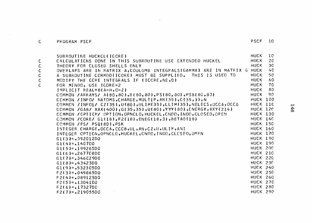
C PROGRAM PSCF
SUBROUTINE HUCKCL(ICCRE) C CALCULATICNS DONE IN THIS SUBROUTINE USE EXTENDED HUCKEL C THEORY FOR CLOSED SHELLS ONLY C OVERLAPS ARE IN MATRIX A,COULOMB INTEGPALS(GAMMA) ARE IN MATRIX C A SUBROUTINE CORMOD(ICORE) MUST BE SUPPLIED. THIS IS USED TO C MODIFY THE CCRE INTEGRALS IF (ICORE.NE.Q) C FOR MINOO, USE ICORE=2
IMPLICIT REAL*8(A-H,C-Z) COMMON /ARRAYS/ A(80,80),B(B0,80),PS(80,80),PSB(8C,80) CCMMON /INFO/ NATOMS,CHARGE,MULTIP,AN{35),C(35,3),N COMMCN /INFO!/ CZ(35),U(80),ULIM{35),LLIM(35),NELECS,OCCA,OCCB CCMMON /GAB/ XXX(400),G(35,35),Q(80),YYY(80),ENERGY,XXY(214) CCMMON /CPTICM/ OPTION,OPNCLO,HUCKEL,CNDO,INDO,CLOSED,OPEN COMMON /CORE/ Gl(l6),F2(18),ENEG(18,3),BETA0(18) CCMMON /PS/ PSQ(80),PSK INTEGER CHARGE,OCCA,CCCB,UL,AN,CZ,U,ULIM,ANI INTEGER CPTICN,OPNCLO,HUCKEL,CNDO,INDO,CLCSED,ODFN Gl(3)=.)92012DO GlC4)=.140700 G l( 5 )= .19926500 Gl(6)=.267708DC G lC 7 )=. 346C2 9DO Gl(B)=.4342300 Gl(9)=.532305DO F2(3)=.049865DO F2(4)=.08912500 F2(5)=.13041DO F2(6)=.17327DO F2(7)=.219055DO
PSCF 10
HUCK l (' HUCK 20 HUCK 30
G HUCK 't0 HUCK 50 HUCK 60 HUCK 70 HUCK 80 HUCK 90 HUCK 100 HUCK llC
"""' HUCK 120 ~ O')
HUCK 130 HUCK 14C HUCK 150 HUCK 160 HUCK 170 HUCK 180 HUCK 190 HUCK 20C HUCK 210 HUCK 220 HUCK 23C HUCK 240 HUCK 250 HlJCK 260 HUCK 270 HUCK 280 HUCK 290

F2(8)=.266415DO HUCK 30(, F2(9)=.3158000 HUCK 31C ENEG(l,1)=7.176100 HUCK 320 ENEG(3,1)=3.1055DO HUCK 330 ENEG(3,2)=1.258DO HUCK 340 E~EG(4,1)=5.94557DO HUCK 350 ENEG(4,2)=2.56300 HUCK 360 ENEG(S,1)=9.5940700 HUCK 370 ENEG(5,2)=4.CG100 HUC'< 380 ENEG(6,l)=l4.051DO HUCK 390 ENEG(6,2)=5.57200 HUCK '•OC ENEG(7,1)=19.31637DO HUCK 410 ENEG(7,2)=7.275DO HUCK 420 ENEG(8,1)=25.39017DO HUCK 430 f--1
ENEG(B,2)=9.11100 HUCK 4'tC' ii::,. -.;J
E~EG(9,1)=32.2724DC HUCK 450 ENEG(9,2)=11.0800 HUCK 460 ENEG(ll,1)=2.804DO HUCK 470 ENEG(ll,2)=1.302DO HUCK 480 ENEG(ll,3)=0.150DO HUCK 49C ENEG(l2,1)=5.1254DO HUCK 500 ENEG(12,2)=2.0516DO HUCK 510 ENEG(l2,3)=0.16195DO HUCK 520 ENF.G(13,1)=7.7706DO HUCK 530 ENEG(l3,2)=2.9951DO HUCK 540 ENEG(13,3)=0.22425DO HUCK 550 ENEG(14,1)=1C.0327DO HUCK 560 ENEG(14,2)=4.1325DO HUCK 570 ENEG(l4,3)=0.337DO HUCK 58C ENEG(lS,1)=14.032700 HUCK 590 ENEG(15,2)=5.4638DO HUCK 600 ENEG(lS,3)=0.50000 HUCK 610

ENEGll6,1)=17.6496DO HUCK 620 ENEG(l6,2)=6.98900 HUCK 63C ENEG(l6,3)=0.71325DO HUCK 640 ENEG(l7,1)=21.5906DO HUCK 650 ENEG(17,2)=8.708100 HUCK 66C ENEG(17,3)=0.S7695DO HUCK 670 B!:TAO( U=-9.DO HUCK 680 BETA0(3)=-9.DO HUCK 690 BETA0(4)=-13.0C HUCK 700 BETA0{5)=-17.DO HUCK 71(1 RETA0(6)=-21.00 HUCK 720 BET AO( 7)=-25.DO HUCK 730 BF.TA0{8)=-31.DO HUCK 74C Bf:TA0(9)=-39.DO HUCK 75C .... BETAO(ll)=-7.720300 HUCK 760 ii::.
00 BETA0(12)=-9.4471DO HUCK 77C BETAO(l3)=-11.3011DO HUCK 780 BETA0(14)=-13.C65DO HUCK 790 BETAO(l5)=-15.07000 HUCK 800 BETAO(l6)=-18.!50DO HUCK 81C RETA0(l7)=-22.33CD0 HUCK 82( IF (ICORE.NE.O) CALL CCRMOD (!CORE) HUCK 830
C FINO NELECS AND FILL W CORE(DIAGONAL) WITH (!+A)/2 HUCK 84C NELECS=O HUCK 85C DC 50 l=l,NATCMS HUCK 860 NELECS=NELECS+CZ(I) HUCK 870 LL=LLIM( I) HUCK €80 UL=ULIM(I) HUCK 890 AN I= AN ( I ) HUCK 900 L=O HUCK 910 DO 40 J=LL,UL HUCK 92C L=L+l HUCK 930

20
C
30
C C
C
40 50
C
IF (L.EQ.l) GO TO 30 HUCK 940 IF (L.LT.5) GO TO 20 HUCK 950 A(J,J)=-ENEG(ANI,3)/27.21DO HUCK 96C PS(J,J)=-3.DO*(A(J,J)-(DFLOAT(CZ(I))-.SDO)*G(I,I)) HUCK 97C GO TO 40 HUCK 980 A(J,J)=-ENEG(ANI,2)/27.2100 HUCK 990 PS(J,J)=-3.DO*(A(J,J)-(OFLOAT(CZ(I))-.SDC)*G(I,I)) HUCKlOOO MINDG CORRECTICN FOR P-ORBITALS HUCK1010 IF (ICORE.EQ.2) A(J,J)=A(J,J)+0.5D0*G(I,I)+Gl(ANI)*(DFLOAT(CZ(I)-1HUCK1020
l)/6.0DO-l.CD0)/3.0DO+F2(ANI)*(0.28D0/3.0DL*DFLOAT(CZ(I)-l)-O.OBDO*HUCK103Q 2(QFLOAT(CZ(I))-2.5DO)) HUCK104C
GO TO 40 HUCK1050 A(J,J)=-ENEG(ANI,1)/27.2100 HUCK106G PS(J,J)=-3.DO*(A(J,J)-(DFLOAT(CZ(I))-.5DC)*G(I,I)) HUCK107( MINDO CORRECTION FORS-ORBITALS HUCK1080 H ATOMS HUCK109f IF (ICORE.EQ.2.AND.ANI.EQ.l) A(J,J)=A(J,J)+0.500*G(J,I) HUCKllOO OTHER ATOMS THANH HUCKlllO IF (ICORE.EQ.2.AND.ANI.NE.l) A(J,J)=ACJ,J)+0.5D1*G(I,I)+Gl(ANI)/12HUCKI120
1 .ODO HUCK 1130 CCNTINUE HUCK1140 CONTINUE HUCK115C NELECS=NELECS-CHARGE HUCK1160 OCCA=NELECS/2 HUCK1170 FORM HUCKEL HAMILTONIAN IN A (OFF DIAGONAL TWO CENTE~ TERMS) HUCKllBO DO 90 I=2,N HUCK119C K=U( I) HUCK12CO L=ANCK) HUCK1210 UL=I-1 HUCK1220 DO 90 J=l,UL HUCK1230 KK=U ( J) HUCK 1240 LL=AN(KK) HUCK1250
I-' ~ co

C
60
70
80
90 C
1(•0
C
C
110
120
IF ((L.GT.9).0R.(LL.GT.9)} GO TO 80 IF ( ICORE.NE.2) GO TO 60 MINDO BETAS A(l,J)=A(I,J)*A(J,l) GO TO 70 PS(1,J)=C.75DO*A(I,J)*(PS(l,I}+PS(J,J))/2.0D0 ACI,J)=A(I,J)*(BETAO(L)+BETAO(Ll))/54.4200 PS(J,I)=PS(I,J) A(J, I)=A( I,J) GO TO 90 P S ( 1 , J ) = 0 • 7 5 DO* A ( I , J ) * ( PS ( I , I ) +PS < J , J ) ) / 2. 0 D 0 A(1,J)=0.75CDO*A(I,J)*(BETAO(L)+BETAO(LL))/54.42DO PS(J,I )=PS( I,J) A ( J , I ) =A ( I , J ) CONTINUE OFF DIAG TERMS CALCO BY A WOLFSBERG-HfLMHOLTZ METHon DO 100,I=l,N Q ( I ) =A ( I , I ) RHO= 1. D-8 CALL EIGN (N,RHO) EIGENVECTORS(IN e) ARE CONVERTED INTO DENSITY MATRIX(IN B) CALL DEN (OCCA,2,N) ADD V(AB) TO HCORE--CNDO 0 0 120 I= l , N J=U ( I) Q( I )=Q( I )+C.SDO*G( J,J) DO 110 K=l,NATOMS IF (K.EQ.J) GO TO 110 PS(I,I)=PS(I,I)+DFLOAT(CZ(K)»*G(J,K) Q(I)=Q(I)-DFLOAT(CZ(K))*G(J,K) PSQ(l)=PS(I,I) CONTINUE
HUCK1260 HUCK1270 HUCK1280 HUCK129C HUCK13GO HUCK1310 HUCK1320 HUCK133C HUCK1340 HUCK1350 HUCK1360 HUCK1370 HUCK1380 HUCK139C HUCK140C HUCK1410 HUCK1420 HUCK143C HUCK 144( HUCK1450 HUCK1460 HUCK1470 HUCK148C HUCK1490 HUCK1500 HUCK1510 HUCK 1520 HUCK1530 HUCK1540 HUCK1550 HUCK1560 HUCK1570
f--1 CJ1 0

C
C
130
140
150
160 170
180 190 200
210 220
EXIT SEGMENT IF ONLY CNDO APPROXIMATIONS ARE DESIRED IF (OPTION.EQ.CNDO) GO TO 200 I~DO MODIFICATION(CORRECTION TO U(I,I)) Du 190 I=l,NATGMS K=AN(I) J=LLIM(I) IF ((K.GT.lJ.ANO.(K.LT.10)) GO TO 130 GO TO 190 IF (K.LE.3) GO TO 140 Q(J)=Q(J)+(OFLOAT(CZ(l))-l.SDO)*Gl(K)/6.DO IF (K.EQ.3) GO TO 160 IF (K.EQ.4) GO TO 150 TEMP=Gl(K)/3.DO+(DFLOAT(CZ(I))-2.500)*2.00*F2(K)/25.0J GC TO 170 TEMP=Gl(K)/4.DO GC TO 170 TEMP=Gl(K)/12.DO CCNTINUE DO 180 L=l, 3 Q(J+L)=Q(J+L)+TEMP CCNTINUE CCNTINUE DJ 220 I=l,N DO 210 J=I,N PS B ( I, J) = 0. GOO PSB(J,I)=PSB(I,J) A ( J , I ) =A ( I , J ) A ( I , I ) =Q ( I ) wRITE (6,230) CALL SCFOUT (0,1) WRITE (6,240) CALL SCFGUT (0,3)
HUCK158G HUCK159C HUCK160C• HUCK1610 HUCK162C HUCK1630 HUCK1640 HUCK1650 HUCK166C HUCK1670 HUCK1680 HUCK1690 HUCK170C HUCK1710 HUCK1720 HUCK173C HUCK1740 HUCK1750 HUCK1760 HUCK1770 HUCK 1780 HUCK1790 HUCKlAOC HUCK 181(, HUCK182C HUCK1830 HUCK1840 HUCK185C HUCK1860 HUCK lfl 7( HUCK1880 HUCK1890
I-' 01 I-'

C 230 240 250
WRITE (6,250) RETURN
FORMAT (1X,28H ELECTRONIC CQRE HAMILTONIAN/) FORMAT (1X,29H POSITRONIC COR.E HAMILTONIMI /) FORMAT (1X,73H INITIAL ELECTRON DENSITY MATRIX A~O EIGENVALUES
lCULATED FROM HCORE(-)/) END
HUCK1900 HUCK191G HUCK1920 HUCK193C-HUCK1940
CALHUCK195(; HUCK196C HUCK1970
I-' c.n I.\J

SUBROUTINE DEN (IOCC,MOP,N) DENS lC IMPLICIT REAL*B(A-H,O-Z) DENS 2( COMMON /ARRAYS/ A(B0,80,4) DENS 30 DIMENSION X(400) DENS 40 L =1 DENS 50 IF ( IOCC .GT .1) L=2 DENS 60 DO 40 I=l,N DENS 70 0020J=I,N DENS 80 X{J)=0.000 DENS 90 DO 10 K=l,IOCC DENS lOC
10 X(J)=X(J)+l*A(I,K,MOP)*A(J,K,MOP) DENS llC 20 CCNTINUE DENS 120
DO 30 J=I,N DENS 130 30 A ( I , J , MO P ) = X ( J J DENS 140 ..... 40 CCNTINUE DENS 15C C.11
DO 50 I=l,N DENS 160 c.,
DD 50 J=I,N DENS 170 50 A ( J , I , MOP ) = A ( I , J , MOP ) DENS 180
RETURN DENS l9C ENO DENS 210

C C C C
20
30
SUBRCUTINE SCFCLO CNDO/INDG CLOSED SHELL SCF SEGMENT GAMMA MATRIX CONTAINED ING, CORE HAMILTCNIAN CONTAINcD IN Q AND UPPER TRIAMGLE OF A, AND INITIAL DENSITY MATRIX CONTAINED IN B CPTIGNS CNOO OR INDO IMPLICIT REAL*8(A-H,O-Z) CCMMON /ARRAYS/ A(80,80),R(B0,8u),PS(80,80),PSg(a0,80) COMMON /INFO/ NATOMS,CHARGE,MULTIP,AN(35),C(35,3),N CCMMON /GAB/ XXX(4CO),G{35,35),Q(80) ,YYY(80),ENERGY,XXY(214) COMMON /INFGl/ CZ(35),U(80),ULIM(35),LLIM(35),NELECS,OCCA,OCCB CCMMON /CPTICM/ OPTION,OPNCLO,HUCKEL,CNDG,INDO,CLOSED,OPEN COMMON /CORE/ Gl(l8),F2(18),ENEG(l8,3),BETAO(l8) CCMMON /PS/ PSQ{80),PSK DIMENSION HELP1(80,80), HELP2(80,80), ${80,80), P(80,80) INTEGER CPTICN,OPNCLO,HUCKEL,CNDO,INDO,CLOSEO,OPEN INTEGER CHARGE,OCCA,OCCB,UL,ULIM,U,AN,CZ,Z l=O IT=99 RHO=l.D-8 DO 20 I=l,N II=U(I) OQ 20 K=l,N JJ=U{K) PS ( I , I)= PS (I, I )-8 ( K, K) *G ( I I, JJ) DO 30 l=l,N DC 30 J=l,N HELP!( I ,J)=A{I ,J) HELP2U,J)=B( I ,J) A( I,J)=PS(I,J) B{I,J)=PSB(I,J) CALL EIGN (N,RHO) CALL DEN (1,2,N)
SCFC 10 SC FC 20 SCFC 3C SCFC 4C SCFC 50 SCFC 60 SCFC 70 SCFC 80 SCFC 9C SCFC 100 SCFC llC SCFC 12(: SCFC 130 SCFC 140 SCFC 150 SCFC 160 SCFC 170 SCFC 180 SCFC 19C SCFC 200 SCFC 210 SCFC 220 SCFC 230 SCFC 240 SCFC 25C SCFC 260 SCFC 270 SCFC 280 SCFC 290 SCFC 300 SCFC 310 SCFC 320
..... Ul ~

WRITE (6,230) SCFC 330 CALL SCFOUT <1,2) SC FC 34C 00 40 I=l,N SC FC 35C• Ou 40 J=l,N SCFC 360 PS(I,J)=A<I,J) SCFC 370 PSB( I,J)=B( I ,J) SCFC 33C A(l,J)=HELPl(I,J) SCFC 390
40 B(I,J)=HELP2(1,J) SCFC 400 50 CCNTINUE SCFC 410
Z=Z+l SCFC 420 ENERGY=0.000 SCFC 43C 00 60 I=l ,N $CFC 440 ACI,I)=Q(I) SCFC 45C PSCI,I)=PSQ(I) SCFC 460 I-'
DO 60 J=I,N SCFC 470 c.n c.n S(I,J)=B(I,J) SCFC 480 SCJ,I)=S(I,J) SCFC 490 P ( I , J) =PS 8 ( I , J) SC FC 500 P(J,I)=P(I,J) SCFC 510
60 A(J,I>=A(l,J) SCFC 520 DO 70 I=l,N SCFC 530 II=U(I) SCFC 540 A(I,I)=A(I,I)-B(I,I)*G(II,II)*0.5DO SCFC 55C DCJ 70 K=l,N SCFC 560 JJ=U(K) SCFC 570 PS(l,I)=PS(l,1)-B(K,K)*G(Il,JJ) SCFC 58C
70 A(I,l)=A(I,l)+B(K,K)*G(II,JJ)-PSB(K,K)*G(Il,JJ) SCFC 59C N'-1=N-l SCFC 600 DC 80 I=l,NM SCFC 610 II=U(I) SCFC 62(• LL= I +l SCFC 63(; DO 80 J=LL,N SCFC 640

JJ=U ( J) SCFC 650 80 A(J,l)=A(J,I)-B(J,I)*G(Il,JJ)*0.5DO SCFC 66C C INDO MODIFICATION SCFC 670
IF (OPTICN.E,.CNDO) GO TO 110 SCFC 68C DO 100 11=1,NATOMS SCFC 690 K=AN (II) SCFC 70C I=LLIM(II) $CFC 710 IF (K.EQ.l) GO TO 100 SCFC 720 PAA=B( I,I)+B(l+l,I+l)+B(I+2,I+2)+B(l+3,I+3) SCFC 73( A(I,I)=A(I,I)-(PAA-B(I,I))*Gl(K)/6.DO SCFC 740 DO 90 J=l,3 SCFC 750 A(I+J,I+J)=A(I+J,I+J)-BCI,I)*Gl(K)/6.0C-(PAA-B(I,I))*7.00*F2(K)/50SCFC 760
l.DO+B(I+J,I+J)*ll.DO*F2(K)/50.DO SCFC 770 90 A(I+J,I)=A(l+J,I)+B(I,l+J)~Gl(K)/2.00 $CFC 780
I l= I +l SCFC 790 I2=1+2 SCFC 800 13=1+3 SCFC 810 A{I2,Il)=A( I2,Il)+B(I2,Il)*ll.D0*F2(K)/50.DO $CFC 820 A(I3,Il)=A(I3,Il)+B( 13,Il)*ll.D0*F2(K)/50.DO SCFC 830 A(I3,I2)=A(I3,I2)+B(I3,I2)*ll.DC*F2(K)/50.DO $CFC 840
100 CCNTINUF. SCFC 850 110 CONTINUE SCFC 860
DO 12J 1=1,N SCFC 870 KK=U(I) SCFC 880
120 ENERGY=ENERGY+.5DO*B(I,I)*(A{I,I)+Q(I))+.5DO*PSB(I,I)*(PS(I,I)+PSQSCFC 89C l(I)) $CFC qco
OQ 130 I=l,NM SCFC 910 II=LJ(I) SCFC 920 LL=I+l $CFC 930 DO 130 J=LL, N SCFC 940 JJ=U(J) SCFC 950
1 3 0 E t J ER GY = i: N ER G Y + B ( I , J ) * ( A ( I , J ) + A ( J , I ) ) + P S B ( I , J l * ( P S ( I , J ) + P S ( J , I ) ) SC F C 9 6 C
f--1 c.n m

W~ITE (6,240) ENERGY SCFC 970 IF (DABS(ENERGY-OLDENG).GE.l.000-6) GO TO 140 SCFC 98C Z=lCO SCFC 0 90 WRITE (6,250) SCFClOOC GO TO 150 SCFC HHO
140 CCNTINUE SCFC1020 OLDENG=ENERGY SCFC 1030
150 CONTINUE SCFC 1C40 IF (Z.LE.IT) GO TO 170 SCFC1050
C SYMMETRIZE F FCR PRINTING (MATRIX A) SCFC l'.)60 DO 16J I=l,N SCFC1C'70 DO 160 J= I, N SCFC1080
160 A( I ,J)=A(J, I) SCFC 1C9'} WRITE (6,260) SCFCllOO f-,J
CALL SCFCUT (0,1) SCFClllO CJl
W~ITE (6,270) SCFC1120 --::i
CALL SCFOUT (0,3) SCFC1130 170 CCNTINUE SCFC 1140
C~LL EIGN (N,RHO) SCFC115C IF (Z.LT.IT) GO TO 180 SCFC1160 W~ITE (6,280) SCFC:1170 CALL SCFGUT ( 1, 2) SCFC118C
180 DO 190 I=l,N SCFC119C' D:J 190 J=l,N SCFC 120C· hELPl(I,J)=A(I,J} SCFC1210 HtLP2(1,J)=e(I,J) SCFC 1220
190 A(l,J)=PS(I,J) SCFC1230 CALL EIGN (N,PHO) SCFC124C DO 200 I=l,N SCFC1250 DO 200 J=l,N SCFC1260 PS( I ,J):A(I ,J) SCFC1270 PSB(I,J)=B(I,J) SCFC1280

200
210 C
220
C 230
240 250 260 270 280 290
A(I,J)=HELPl(I,J) B(I,J)=HELP2(I,J) IF (Z.LE.IT) GO TO 210 WRITE (6,290) CALL SCFOUT (1,4) CONTINUE EIGENVECTORS ( IN B ) ARE CCNVERTED INTO Oi=NSITY MATRIX ( IN B) CALL DEN (OCCA,2,N) CALL DEN (1,4,N) DO 220 I=l,N DO 220 J=l,N PSB( I,J)=O.SDO*(PSB( I,J)+P( I,J)) B ( I , J) =O. 500* ( B ( I, J) +S ( I, J) ) IF (Z.LE.IT) GO TO 50 RETURN
FORMAT (1X,69H INITIAL POSITRON DENSITY MATRIX AND EIGENVALUES lCULATED FROM F(+)/)
FORMAT (//,10X,21H ELECTRONIC ENERGY ,Fl6.10) FJRMAT (5X,18H ENERGY SATISFIED/) FORMAT (1X,36H ELECTRON HARTREE-FOCK ENERGY MATRIX/) FORMAT (1X,36H POSITRON HARTREE-FOCK ~NERGY MATRIX/) FCRMAT (1X,33H ELECTRON EIGENVALUES AND VECTORS/) FORMAT (1X,33H PCSITPON EIGENVALUES AND VECTORS/) ENO
SCFC129C SCFC130C SCFC131C SCFC1320 SCFC1330 SCFC134C SCFC135C SCFC1360 SCFC1370 SCFC1380 SCFC1390 SCfC1400 SCFC141C SCFC1420 SCFC143C SCFC1440
CALSCFC1450 SCFC 1460 SCFC 14 70 SCFC1480 SCFC1490 SCFC1500 SCFC1510 SCFC1520 SCFC153C
1-1 U1 00

C
10
SUBROUTINE CPRINT IMPLICIT REAL*8(A-H,O-Z)
CNDG-INDO SCF CLOSED SHELL - PRINTOUT CCMMON /ARRAYS/ A(80,80),B(80,80),D(80,80),PS8(80,80) COMMON /GAB/ XXX(400),G(35,35),Q(80),YYY(80),ENERGY,XXY(214) COMMON /INFO/ NATOMS,CHARGE,MULTIP,AN(35),C(35,3),N COMMON /INFOl/ CZ(35),U(80),ULIM(35) ,LLIM(35),NELECS,OCCA,OCCB CCMMON /PERTEL/ EL(l8) CO~MON /CPTICM/ OPTION,OPNCLO,HUCKEL,CNOC,INOO,CLOSED,OPEN CCMMON /ORB1/ ORB(9) INTEGER CPTIGN,OPNCLO,HUCKEL,CNDO,INDO,CLGSEO,OPEN INTEGER CHARGE,OCCA,OCCB,UL,ULIM,U,AN,CZ,Z,EL,ANI,ORB INTEGER ULI,ULJ DIMENSION DP~(3), OM(3), DMSP(3), OMP0(3) DIMENSION ATENG(l8) IF (OPTION.EQ.CNDO) GO TO 10 ATENG{l)=-0.638730246200 ATENG(3)=-.2321972405DC ATENG{4)=-l.121962035400 ATENG(S)=-2.872575004800 ATENG(6)=-5.934954826100 ATENG(7)=-10.673174125100 ATENG{B)=-17.292085065000 ATENG(9)=-26.257437787500 GO TO 20 CONTINUE ATENG(l)=-0.638730246200 ATENG(3)=-.232197240500 ATENG{4)=-l.145412035500 ATENG{S):-2.977423904800 ATENG(6)=-6.l64993626100 ATENG{7)=-11.0768746252DO
CPRT 10 CPRT 2(' CPRT 30 CPRT 4C CP'<.T 50 CPRT 6C (DRT 70 CPRT 80 CDRT 9C CPRT lJO CPRT 110 CDP.T 120 CPRT 13C CPRT 14(' CPRT 150 CPRT 160 CPP.T 17(' CPRT l BC• CPRT 19C CPRT 2'.)0 CPRT 210 CPPT 22C CPRT 230 CPRT 240 CPRT 250 CPRT 260 CDRT 270 CPRT 280 CPRT zqo CPRT 300 CPQ.T 310 CPRT 32C
I-' c.n (.0

20
30 40
50
ATENG(S)=-18.081965865100 CPRT 330 ATENG(9)=-27.5491302880DO CPRT 340 ATENG(ll)=-.1977009568DO CPRT 350 ATENG(12J=-.8671913833DO CPRT 360 ATENG(l3J=-2.0364557744DO CPRT 37C ATENG(l4)=-3.8979034686DO CPRT 38C ATENG(l5)=-6.7966009163DO CPRT 390 ATENG(l6)=-10.7658174341DO CPRT 40( ATENG(l7)=-16.0467017940DO CPRT 410 CONTINUE CPRT 42C K=NATOMS-1 CPRT 430 WRITE (6,160) CPRT 440 CALL SCFOUT (0,2) CPRT 45G WRITE (6,170) CPRT 460 CALL SCFGUT (0,4) CPRT 470 IF (NATOMS.EQ.l) GO TO 40 CPRT 480 DO 30 I=l,K CPRT 49C L=I+l CPRT 500 DO 30 J=L,NATOMS . CPRT 51C RAD=DSQRT{(C(I,1)-C(J,1))**2+(C(I,2)-C(J,2))**2+(C(I,3)-C(J,3))**2CPRT 520
1) CPRT 530 ENERGY=ENERGY+(DFLOAT(CZ(I))*DFLOAT(CZ(J)))/RAO CPRT 540 WRITE (6,180) ENERGY CPRT 550 DO 50 I=l,NATOMS CPRT 560 A N I = AN ( I ) C PR T 5 7 0 ENERGY=ENERGV-ATENG(ANI) CPRT 580 WRITE (6,190) ENERGY CPRT 590 WRITE (6,200) CPRT 600 DO 70 I=l,NATOMS CPRT 610 TCHG=O.DO CPRT 620 PSCH=O.ODO CPRT 630 LL= L L I M ( I ) CPR T 6 40
t-J O') 0

UL=Ull M( I) CPRT 650 DO 60 J=LL,UL CPP.T 660 PSCH=PSCH+PSB(J,J) CPRT 670
60 TCHG=TCHG+B(J,J) CPRT 680 AN I = AN ( I ) C PR T 6 9 0 WRITE (6,210) 1,EL(ANI),TCHG,PSCH CPRT 700 XXX (I) =TCHG CP~T 7 lC
70 CONTINUE CPRT 720 D1] 80 I=l,3 CPRT 730 OM( I )=O.COO CPRT 740 OMSP(I)=0.00 CPRT 750
80 OMPO(l )=C.00 CPRT 760 DO 140 J=l,NATGMS CPRT 770 IF (AN(J).LT.3) GO TO 120 CPRT 780 IF (AN(J).LT.11) GO TO 100 CPRT 790 SLTR1=(.65DO*DFLOAT(AN(J))-4.95D0)/3.DO CPRT 800 FACTOR=2. 541600*7. DO/ ( DSQRT ( 5. DO) *SL TR 1) CPRT 8 lG INDEX=LLIM(J) CPRT 82C DO 90 K=l,3 CPRT 830
90 DMSP(K)=DMSP(K)-B(INDEX,INDEX+K)*l0.2717500/SLTRl CPRT 840 OMPD(l)=DMPD(l)-FACTOR*(B(INDEX+2,INDEX+8)+B(INDEX+3,INDEX+5)+B(INCPRT 850
1DEX+l,INDEX+7)-l.DO/DSQRT(3.DO)*B(INDEX+l,INDEX+4)) CPRT 860 OMP0(2)=DMPD(2)-FACTOR*(B(INDEX+l,INOEX+8)+B(INDEX+3,INDEX+6)+B(INCPRT 870
1DEX+2,INDEX+7)-l.D0/0SQRT(3.DO)*B(INDEX+2,INDEX+4)) CPRT 880 DMPD(3)=DMP0(3)-FACTOR*(8(INOEX+l,INDEX+5)+B(INDEX+2,INDEX+6)+2.00CPRT 890
l/0SQRT(3.DO)*B(INDEX+3,INDEX+4)) CPRT 900 GO TO 120 CPRT 91(1
!CO INDEX=LL H' ( J) CPRT 920 DO 110 K=l, 3 CPRT 930
110 O~SP(K)=DMSP(K)-B(INOEX,INDEX+K)*7.33697DC/(.325D0*DFLOAT(AN(J)-l)CPRT 940 1) CPRT 950
120 DO 130 I=l,3 CPRT 960
I-' m I-'

130 140
150
C 160 170 180 190 200 210 220 230 240 250 260 210 280
DM(l)=DM(I)+(DFLOAT(CZ(J))-XXX(J))*C(J,1)*2.541600 CCNTINUE DO 150 I=l,3 DPM(I)=DM(I)+DMSP(I)+DMPD(I) WRITE (6,220) W~ITE (6,230) WRITE (6,240) OM(l),OM(2),0M(3) WRITE (6,250) DMSP(l),DMSP(2),DMSP(3) WRITE (6,260) DMPD(l),DMPD(2),DMPD(3) WRITE (6,270) OPM(l),DPM(2),0PM(3) DP=DSQRT(DPM(l)**2+DPM(2)**2+0PM(3)**2) WRITE (6,280) OP RETURN
FORMAT (1X,24H ELECTRON DENSITY MATRIX/) FORMAT (1X,24H POSITRON DENSITY MATRIX/) FCRMAT (//,10X,16H TOTAL ENERGY= ,F16.10) FORMAT (//,10X,l6HBIN0ING ENERGY= ,Fl6.10,5H A.U./) FORMAT (10X,32H(-)CHG DENSITY (+)CHG DENSITY) FORMAT (I3,A4,8X,F7.4,l1X,F7.4) FORMAT (//,20X,16H DIPOLE MOMENTS,/) FCRMAT (5X,11H CCMPONENTS,3X,2H X,8X,2H Y,8X,2H Z) FORMAT (5X,10H DENSITIES,3(1X,F9.5)) FORMAT (5X,4H S,P,6X,3(1X,F9.S)) FORMAT (5X,4H P,D,6X,3(1X,F9.5)) FORMAT (5X,6H TOTAL,4X,3(1X,F9.5),/) FORMAT (3X,15H DIPOLE MOMENT=,F9.5,7H DEBYES,//) END
CPRT 97C CPRT 980 CPRT g9c CPR T 1000 CPRT1010 CPRT102C (PRT1030 CPRT 1040 CPRT1050 CPRT1060 CPRT1070 CPRT1080 CPRT1C9C CPRTllOG CPRTlllO CPRT112C CPRT 1130 CPRT 1140 CPRT1150 CPRT1160 CPRT117C CPRT1180 CPRT1190 CPRT 1200 CPRT1210 CPRT1220 CPRT123C CPP.T 1240
1-J 0) I).:,

C C C C C C
C C
20
30 C C
PROGRAM PAL PAL 10 A PROGRAM FOR THE ANALYSIS OF DECAY CURVES PAL 20 VERSION FOR IBM.360 . PAL 30 INCLUDING AN ITERATIVE PROCEDURE FOR DETERMINATION OF HALF LIVES PAL 40 WITH REVISED RJT ROUTINE. - CAUSES OLD ROUTINE TO BE USED. PAL 50 USING DOUBLE PRECISION INVERSION ROUTINE BNSINV PAL 60 DOUBLE PRECISION 8(10,10) PAL 70 DOUBLE PRECISION U(l0,10),BR(l0,10) PAL 80 DOUBLE PRECISION T(512l,F(512),SFSQ(512),H(l0),D(lO),A(512,10),APFPAL 90
l(lO),FCALC(512),SF(200),SIGMAH(lO),X(lO),SIGMAD(lO),DELTAD(l0,9),DPAL 100 2DELTA(l0,9),XPOTO(lO),XE08(10),SXEOB(lO),UNITK(lO),TAU(lO),ANN(lO)PAL 110
DOUBLE PRECISION BADT(512),BADFS(512),BINVRS(10,10),FKCS(5),SFKCS(PAL 120 15),RATI0(512),V(512) PAL 130
DOUBLE PRECISION DT,DABS,DSQRT,OEXP PAL 140 EQUIVALENCE (BADT,SF), (BADFS,V), (BINVRS,B) PAL 15C DIMENSION AA(5), SLOP(5), YCAL(512) PAL 160 DIMENSION CCMNT(8), NAME(ll), JUNIT(lO) PAL 170 INTEGER HR,DAY,YR PAL 180 INTEGER CMIT PAL 190 DATA HR,OAY,YR/lHH,lHO,lHY/ PAL 200 READ (5,890) COMNT PAL 210 ENTRANCE TO PROGRAM PAL 220 INPUT PAL 230 AIM=O.O PAL 240 L Tl=O PAL 250 READ (5,890) IDENT,NAME,IENDS PAL 260 IF (lENDS.EQ.O) GO TO 40 PAL 270 IF (AIM.EQ.O.O) GO TO 30 PAL 280 CALL PLOT {0.0,0.0,-4) PAL 290 CALL EXIT PAL 300 NC IS NO. OF COMPONENTS PAL 310 NV IS NO. OF UNKNOWN HALF LIVES PAL 320
I-' en c..,

C C C C C C C C C C C C C C C C C C C C C C C C C C C C 40
50
NCNV ALWAYS EQUALS ONE PAL CNV GOVERNS HOW FAR ITERATIONS WILL PROCEED; IF CNV IS ZERO A PAL
MAX. OF NINE ITERATIONS WILL BE PERFORMED PAL BGD IS THE COUNTER BACKGROUND FOR SUBTRACTION PAL SBGD IS THE STANDARD DEVIATION FOR ROOT-MEAN-SQUARE ADDITION TO PAL THE STANDARD DEVIATION OF EACH POINT (USUALLY ZERO) PAL IN ••• INPUT CONTROL (ZERO OR BLANK CAUSES USE OF PROGRAM INPUT PAL
FORMAT; POSITIVE INTEGER TRANSFERS TO SUBROUTINE INPUT) PAL IT ••• NUMBER HERE CAUSES INTERMEDIATE MATRICES TO BE PRINTED PAL
(USUALLY LEFT BLANK) PAL BLOCK IS THE COUNTER DEAD TIME (USUALLY LEFT BLANK) PAL SCOFF IS CUTOFF (IN PERCENT) ON THE SMALLEST VALUE AT WHICH THE PAL PROGRAM WILL USE THE STANDARD DEVN. FROM STATS. ALONE (0.5) PAL RJT ••• IF NOT BLANK OR ZERO PROGRAM EXAMINES ITS OUTPUT ANO PAL REJECTS POINTS WHICH FALL FURTHER THAN RJT TIMES THE STANDARD PAL DEVN. FROM THE CURVE. THE FIT IS THEN REPEATED PAL KCS ••• CAUSES THE PROGRAM TO ENTER A KNOWN COMPT. SUBTRACTION PAL
ROUTINE (USUALLY SET AT ZERO» PAL ICARD IF UNECUAL TO ZERO CAUSES PROGRAM TD ENTER INTENSITY PAL
ROUTINE (USUALLY EQUALS ZERO) PAL INP ••• IF EQUAL TO ZERO OR BLANK ALLOWS HALF-LIFE GUESSES TO BE PAL ENTERED AS HALF-LIVES AFTER TIME-PER-CHANNEL CORRECTION; IF PAL EQUAL TO ONE ALLOWS TAU GUESSES TO BE USED PAL OMIT ••• OATA OUTPUT OPTIONS PAL
READ (5,900) lRD,INP,OMIT
OMIT=l:OUTPUT INCLUDES ALL DATA, INCLUDES GRAPH PAL OMIT=2:0MITS SUPERFLUOUS DATA, INCLUDES GRAPH PAL OMIT=3:INCLUDES ALL DATA, OMITS GRAPH PAL OMIT=4: OMITS SUPERFLUOUS DATA, OMITS GRAPH PAL
NC,NV,NCNV,CNV,BGD,SBGD,IN,IT,BLOCK,SCOFF,RJT,KCS,ICAPAL PAL
IF (OMIT) 50,50,60 WRITE (6,910)
PAL PAL
330 340 350 360 370 380 390 400 410 420 430 440 450 460 470 480 490 500 510 520 530 540 550 560 57G 580 590 600 610 620 630 640
1--' m ~

GO TO 30 PAL 650 60 IF (OMIT-5) 70,50,50 PAL 660 70 IF (INP.EQ.O) GO TO 90 PAL 670
READ (5,920) CALIB PAL 680 DO 80 1=1,NC PAL 690 READ (5,920) TAU(I),JUNIT(I) PAL 700 H(I)=(TAU(l)*0.69314718)/CALIB PAL 710
80 O(I)=0.69314718/H(I) PAL 720 GO TO 110 PAL 730
90 DO 100 1=1,NC PAL 740 READ (5,920) H(l),JUNITll) PAL 750
C HALF LIFE INPUT CONVERSION. H,D, ORY ~RE RECOGNIZED AS SUCH. PAL 760 C OTHER CHARACTERS ARE TAKEN TO MEAN M. PAL 770
UNITK(I)=0.6931471800 PAL 780 IF (JUNIT(I).EQ.HR) UNITK(l)=0.11552453D-l PAL 790 f--'
O') IF (JUNIT(I).EQ.DAY) UNITK(l)=0.481352210-3 PAL 800 CJl
IF (JUNIT(I).EQ.YR) UNITK(IJ=0.13178987D-5 PAL 810 D(l)=UNITK(l)/H(I) PAL 820
100 CONTINUE PAL 830 110 NP=O PAL 840
NSCHAN=O PAL 850 C INPUT OPTION PAL 860
IF (IN.EQ.O) GO TO 120 PAL 870 CALL INPUT (T,F,SFSQ,NP,BGO,NSCHAN) PAL 880 GO TO 130 PAL 890
120 NP=NP+l PAL 900 READ (5,930) T(NP),F(NP),SFSQ(NP) PAL 910 IF (SFSQ(NP).NE.O.) GO TO 120 PAL 920
C TIME NORMALIZATION PAL 930 130 DO 140 1=2,NP PAL 940
T( I J=T( I >-T( lJ PAL 950 140 CGNTINUE PAL 960

C
150 160
170 C 180
190 C 200
T(ll=O.ODO TO-=T(NP) NP=NP-1 NPl=NP NCl=NC IF (8LOCK.EQ.O.) GO TO 160 DEAD TIME CORRECTION DEADT=BLOCK*(l.67E-8) DO l 50 I = 1 , NP F(I)=F(l)/(1.-DEADT*F(I)) IF (8GD.LE.O.) GO TO 180 SBG0SQ=SBGD**2 DO 170 I=l,NP F(I)=F(I)-BGD SFSQ(l)=SFSQ(I)+SBGOSQ SUBROUTINE FOR SIGMA CUTOFF IF CSCOFF.EQ.O.) GO TO 200 SCOFSQ=SCOFF**2/10000. DO 190 1=1,NP TSFSQ=SC0FS0*F(l)**2 IF (SFSQ(l).LT.TSFSQ) SFSQ(I)=TSFSQ CONTINUE KNOWN COMPONENT SUBTRACTION (KCS) ROUTINE IF (KCS.EQ.O) GO TO 240 READ (5,940) (FKCS(IJ,SFKCS(I),I=l,KCS) DO 230 J=l,KCS NO=NC-KCS+J DO 210 I=l,NP FACTOR=DEXP((TO-T(I))*D(ND)) IF ((F(I)-(FKCS(J)*FACTOR)).LE.0.000) GO TO 220 F(l)=F(I)-FKCS(J)*FACTOR SFSQ(I)=SFSQ(I)+(SFKCS(J)*FACTOR)**2
PAL 970 PAL 980 PAL 990 PAL 1000 PAL 1010 PAL 1020 PAL 1030 PAL 1040 PAL 1050 PAL 1060 PAL 1070 PAL 1080 PAL 1090 PAL 1100 PAL 1110 PAL 1120 PAL 1130 PAL 1140 PAL 1150 PAL 1160 PAL 1170 PAL 1180 PAL 1190 PAL 1200 PAL 1210 PAL 1220 PAL 1230 PAL 1240 PAL 1250 PAL 1260 PAL 1270 PAL 1280
f--1 m m

210 220 230
C 240
C 250
C C 260
210 280
290 300
310 C
CONTINUE NP=NP-1 CONTINUE NC=NC-KCS INITIALIZATION AND RETURNS NI TER=-1 IF (NV.EQ.O) GO TO 250 LTl=l NVTEMP=NV NV=O RETURN AFTER FIXED HALF LIFE PASS NT=NC+NV LV=NC+l CALCULATION CF A MATRIX
ALSO RETURN FOR NEXT ITERATION NITER=NITER+l DO 300 I =1,NP DO 280 J=l,NC OT=-0( JI *T< I) IF ((OT).GT.(-34.500)) GO TO 270 A(I,J)=0.000 GO TO 280 A(I,J)=DEXP(OT) CONTINUE IF (NV.LE.O) GO TO 300 DO 290 J=LV,NT K=J-NC A(I,J)=T(I)*A<I,K) CONTINUE IF (IT) 310,320,310 WRITE (6,950) ((A(I,J),J=l,NT),I=l,2) CONSTRUCT MATRIX APF
PAL 1290 PAL 1300 PAL 1310 PAL 1320 PAL 1330 PAL 1340 PAL 1350 PAL 1360 PAL 1370 PAL 1380 PAL 1390 PAL 1400 PAL 1410 PAL 1420 PAL 1430 PAL 1440 PAL 1450 PAL 1460 PAL 1470 PAL 1480 PAL 1490 PAL 1500 PAL 1510 PAL 1520 PAL 1530 PAL 1540 PAL 1550 PAL 1560 PAL 1570 PAL 1580 PAL 1590 PAL 1600
I-' (j) ...;i

C 320
330
340 C 350
360
370
380 C 390
C
400
410
ALSO RETURN AFTER DATA REJECTION DO 330 I=l,NT APF(I)=0.000 DO 330 K=l,NP APF(I)=APF(I)+A(K,I)*F(K)/SFSQ(K) CONTINUE IF (IT) 340,350,340 WRITE (6,950) (APF(I),I=l,NT) CONSTRUCT MATRIX B DO 360 I=l,NT DO 360 J=l,NT B(l,J)=0.000 DO 360 K=l,NP B(I,J)=B(I,J)+A(K,I)*A(K,J)/SFSQ(K) CONTINUE IF (IT) 370,390,370 WRITE (6,950) ((B(l,J),J=l,NT),I=l,NT) DO 380 Kl=l,NT DO 380 KJ=l,NT BR(KI,KJ)=B(KI,KJ) B MATRIX INVERSION EPSIL=O.ODO CALL BNSINV (B,NT,DETERM,EPSIL,ITEST) B MATRIX IS NOW REPLACED BY ITS INVERSE, BINVRS. IF (ITEST.NE.O) GO TO 580 IF CIT) 400,420,400 WRITE (6,950) ((BINVRS(I,J),J=l,NTJ,I=l,NT) DO 410 I = 1 , NT DO 410 J=l,NT U(I,J)=O.ODO DO 410 K=l,NT UtI,J)=U(I,J)+BINVRS(I,K)*BR(K,J)
PAL 1610 PAL 1620 PAL 1630 PAL 1640 PAL 1650 PAL 1660 PAL 1670 PAL 1680 PAL 1690 PAL 1700 PAL 1710 PAL 1720 PAL 1730 PAL 1740 PAL 1750 PAL 1760 PAL 1770 PAL 1780 PAL 1790 PAL 1800 PAL 1810 PAL 1820 PAL 1830 PAL 1840 PAL 1850 PAL 1860 PAL 1870 PAL 1880 PAL 1890 PAL 1900 PAL 1910 PAL 1920
I-' m 00

C 420
430 C
C 440
450 C
460
470
480 490 C 500
510 C
WRITE (6,950) ((U(l,J),J=l,NT),1=1,NT) SOLUTION OF NORMAL EQUATIONS DO 430 I=l,NT X(I)=0.000 DO 430 J=l,NT X(I)=X(I)+BINVRS(I,J)*APF(J) CONTINUE ENTRANCE TO CALCULATIONS FOR OUTPUT(l27) OR ITERATION TESTS(301) IF (NV.NE.O) GO TO 500 CALCULATIONS FOR OUTPUT DATA DO 450 1=1,NC SIGMAH(l)=O.ODO XPDT0(1)=DEXP(-TO*D(I)) HALF LIFE OUTPUT CONVERSION IF (NV.EQ.O) GO TO 580 IF (INP.EQ.O) GO TO 470 DO 460 1=1,NV H(I)=0.69314718/DCI) SIGMAH(I)=H(l)*SIGMAD(l)/O(I) GO TO 490 DO 480 l=l,NV H(I)=UNITK(l)/0(1) SIGMAH(l)=H( U*SIGMAD(I)/0(1) GO TO 580 TESTS FOR COMPLETION OF ITERATION NON=l DO 520 I=l,NV L= I +NC DELTAD(I,NITER)=-X(L)/X(I) DDELTA(I,NITER)=OABS(DELTAD(I,NITER)) IF (OABS(DELTAD(l,NITER)).LT.0.500*DABSfO(I))) GO TO 520 CHANGE IN ThE DECAY CONSTANT CANNOT EXCEED HALF ITS VALUE
PAL 1930 PAL 1940 PAL 1950 PAL 1960 PAL 1970 PAL 1980 PAL 1990 PAL 2000 PAL 2010 PAL 2020 PAL 2030 PAL 2040 PAL 2050 PAL 2060 PAL 2070 PAL 2080 PAL 2090 PAL 2100 PAL 2110 PAL 2120 PAL 2130 PAL 2140 PAL 2150 PAL 2160 PAL 2170 PAL 2180 PAL 2190 PAL 2200 PAL 2210 PAL 2220 PAL 2230 PAL 2240
I-' O} (0
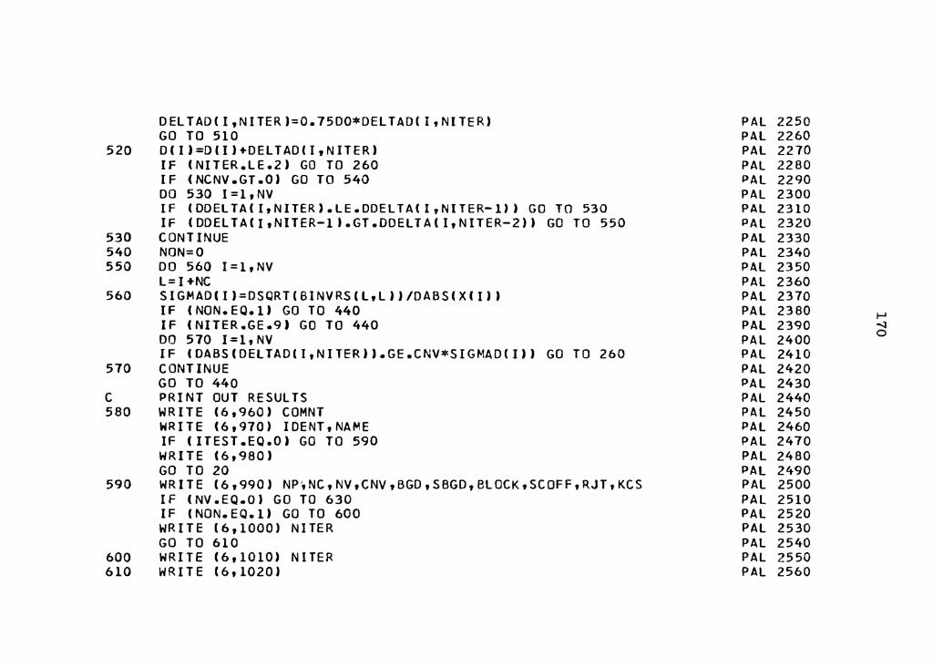
OELTAD(I,NITER)=0.7500*DELTAO(I,NITER) PAL 2250 GO TO 510 PAL 2260
520 O(l)=D(l)+OELTAO(I,NITER) PAL 2270 IF (NITER.LE.2) GO TO 260 PAL 2280 IF (NCNV.GT.0) GO TO 540 PAL 2290 00 530 I=l,NV PAL 2300 IF CODELTA(I,NITER).LE.DDELTA(I,NITER-1)) GO TO 530 PAL 2310 IF CODELTA(I,NITER-11.GT.DOELTA(I,NITER-2)) GO TO 550 PAL 2320
530 CONTINUE PAL 2330 540 NON=O PAL 2340 550 00 560 I=l,NV PAL 2350
L= I +NC PAL 2360 560 SIGMAD(I)=OSQRT(BINVRS(L,L))/DABS(X(I)) PAL 2370
IF (NON.EQ.l) GO TO 440 PAL 2380 f-1 IF (NITER.GE.9) GO TO 440 PAL 2390 -..J 00 570 I=l,NV PAL 2400 0
IF COABS(OELTAD(I,NITER)).GE.CNV*SIGMAD(I)) GO TO 260 PAL 2410 510 CONTINUE PAL 2420
GO TO 440 PAL 2430 C PRINT OUT RESULTS PAL 2440 580 WRITE (6,960) COMNT PAL 2450
WRITE (6,970) IDENT,NAME PAL 2460 IF (ITEST.EQ.0) GO TO 590 PAL 2470 WRITE (6,980) PAL 2480 GO TO 20 PAL 2490
590 WRITE (6,990) NP,NC,NV,CNV,BGD,SBGD,BLOCK,SCOFF,RJT,KCS PAL 2500 IF CNV.EQ.O) GO TO 630 PAL 2510 IF (NON.EQ.l) GO TO 600 PAL 2520 WRITE (6,1000) NITER PAL 2530 GO TO 610 PAL 2540
600 WRITE (6,1010) NITER PAL 2550 610 WRITE (6,1020) PAL 2560

WRITE (6,1030) (0( I) ,I=l,NV) PAL 2570 DO 620 J=l,NITER PAL 2580 WRITE (6,1040) J,(OELTAD(l,J),I=l,NV) PAL 2590
620 CONTINUE PAL 2600 WRITE (6,1050) (SIGMAD(I),l=l,NV) PAL 2610
C CONVERSICN TO EOB PAL 2620 630 DO 640 I=l,NC PAL 2630
XEOB(l)=Xll)*XPOTO(I) PAL 2640 SXEOB(l)=BINVRS(l,I) PAL 2650 IF (I.GT.NV) GO TO 640 PAL 2660 L= I+NC PAL 2670 SXEOB(I)=SXEOB(l)+2.*TO*BINVRS(I,L)+T0**2*BINVRS(L,L) PAL 2680
640 SXEOB(I)=XPDTO(I)*DSQRT(DABS(SXEOB(I))) PAL 2690 DO 650 I=l,NC PAL 2700
650 TAU(I)=(H(I)*CALIB)/0.69314718 PAL 2710 I-' -..J
WRITE (6,1060) PAL 2720 I-'
WRITE (6,1070) (I,H(I),JUNIT(l),SIGMAH(l),JUNIT(I),XEOB(I),SXEOB(IPAL 2730 1 ),XPDTO( I),TAU( I) ,I=l,NC) PAL 2740
IF (KCS.EQ.O) GO TO 670 PAL 2750 l=NC PAL 2760 J=O PAL 2770
660 I=I+l PAL 2780 J=J+l PAL 2790 WRITE C 6, 10 80) 1,Hl I ),JUNIT( I) ,FKCS(J) ,SFKCS(J) PAL 2800 IF (KCS.GT.J) GO TO 660 PAL 2810
670 VPV=O. 0 PAL 2820 DO 690 I=l,NP PAL 2830 FCALC(I)=0.000 PAL 2840 DO 680 J=l,NC PAL 2850 FCALC( I)=FCALC(l)+A( I,J)*X(J) PAL 2860
680 CONTINUE PAL 2870 V ( I ) =F ( I )- FC AL C ( I ) PAL 2880

690
700
710
C
120 730
740 750 760
C
SF(I)=DSQRT(SFSQ(I)) RATIO(I)=V(I)/Sf(I) VPV=VPV+V(l)**2/SFSQ(I) CONTINUE DF=NP-NT FIT=SQRT(VPV/DF) WRITE (6,1090) FIT GO TO (700,710,700,710), OMIT WRITE (6,1100) WRITE (6,1110) (T(I ),F( I>,FCALC( 1),V(I ),SF(I ),RATIO( I) ,I=l,NP) IF (RJT.EQ.O.) GO TO 800 IF (NV.NE.O) GO TO 800 DATA REJECTION SUBROUTINE l=O NRJT=O I=I+l IF CI.GT.NP) GO TO 780 IF (DABSCRATIOCI)).LE.ABS(RJT)) GO TO 720 IF (RJT.LT.O.) GO TO 760 IF (I.EQ.NP) GO TO 750 IF (RATIO(l)*RATIOCl+l)) 740,740,720 IF (I.EQ.l) GO TO 760 IF (RATIO( I )*RATIO( 1-1)) 760,760,720 NRJT=NRJT+l BADT ( NRJT l=H I) BAOFS(NRJT)=F(I) NP=NP-1 MOVE UP REMAINING POINTS DO 770 J=l,NP T( J) =T ( J + l) F(J)=F(J+l) SFSQ(J)=SFSQCJ+l)
PAL 2890 PAL 2900 PAL 2910 PAL 2920 PAL 2930 PAL 2940 PAL 2950 PAL 2960 PAL 2970 PAL 2980 PAL 2990 PAL 3000 PAL 3010 PAL 3020 PAL 3030 PAL 3040 PAL 3050 PAL 3060 PAL 3070 PAL 3080 PAL 3090 PAL 3100 PAL 3110 PAL 3120 PAL 3130 PAL 3140 PAL 3150 PAL 3160 PAL 3170 PAL 3180 PAL 3190 PAL 3200
I-' -.J ~

770
780
790
800
810 820
830
840
850
RATIO(J)=RATIO(J+l) DO 770 K=l,NT A(J,K)=A(J+l,K) CONTINUE GO TO 730 IF (NRJT.NE.O) GO TO 790 WRITE (6,1120) GO TO 800 WRITE (6,1130) NRJT WRITE (6,1140) (BADT(I),BADFS(I),I=l,NRJT) WRITE (6,1150) GO TO 320 IF (LTl.NE.l) GO TO 810 LTl=O NV=NVTEMP GO TO 250 GO TO (820,820,830,830), OMIT CALL POL (F,FCALC,NP,IOENT) AIM=l.O IF (ICARO.EQ.O) GO TO 20 T{l)=-TO STX=T( 1) 00 840 L=2,NP1 T(L)=T(L-1)+1.000 CONTINUE DO 850 K=l,NPl FCALC(K)=0.000 DO 850 J=l,NCl FCALC(K)=FCALC(K)+XEOB(J)*DEXP(-O(J)*T(K)) CONTINUE DO 860 I=l,NPl YCAL(I )=FCALC( I)
PAL 3210 PAL 3220 PAL 3230 PAL 3240 PAL 3250 PAL 3260 P,\L 3270 PAL 3280 PAL 3290 PAL 3300 PAL 3310 PAL 3320 PAL 3330 PAL 334G PAL 3350 PAL 3360 PAL 3370 PAL 3380 PAL 3390 PAL 3400 PAL 3410 PAL 3420 PAL 3430 PAL 3440 PAL 3450 PAL 3460 PAL 3470 PAL 3480 PAL 3490 PAL 3500 PAL 3510 PAL 3520
I-' ..;i w

860
870
C
880
C 890 900 910 920 930 940 950 960 970 980 990
1000 1010 1020
CONTINUE DO 870 1=1,NCl AA(IJ=XEOB(I) SLOP(l)=O(I) CONTINUE CALL INTENS (IOENT,NAME,BGO,STX,NC,NP,AA,SLOP,YCAL,OMIT) CAL. OF ANNIHILATION RATES DO 8 80 I = l , NC ANN(l)=l.O/TAU(I) CONTINUE WRITE (6,1160) WRITE (6, 1170) WRITE (6,1180) WRITE (6,1190) GO TO 20
(TAU(I),I=l,NC) (ANN( I), 1=1,NC) CALIB FIT
PAL PAL PAL PAL PAL PAL PAL PAL PAL PAL PAL PAL PAL PAL PAL PAL
FORMAT (A4,11A4,12J PAL FORMAT (213,I2,F6.4,2F8.2,212,3F5.2,4I2) PAL FORMAT (1Hl,49H PROGRAM FAILURE,DMIT ERROR: DATA CANCELLED) PAL FORMAT (Fl0.5,Al) PAL FORMAT (3El5.8) PAL FORMAT (Fl6.8,Fl4.8) PAL FORMAT (/lH ,9El4.7) PAL FORMAT (1Hl,12A4) PAL FORMAT (1HO,A4,11A4) PAL FORMAT (50HOMATRIX INVERSION HAS FAILED. MORE DATA IS NEEDED.) PAL FORMAT (//4H NP=,I3,4H NC=,12,4H NV=,Il,5H CNV=,F6.4,5H BGD=,F8.2,PAL
16H SBGD=,F8.2,7H BLOCK=,F5.2,7H SCOFF=,F5.2,5H RJT=,F6.4,5H KCS=,IPAL 22) PAL
FORMAT (//25H ITERATIONS PERFCRMED=,I2,15H CONVERGENT) PAL FORMAT (//25H ITERATIONS PERFORMED=,I2,15H NONCONVERGENT) PAL FORMAT (//86H 1ST COMP 2ND COMP 3RD COMPAL
3530 3540 3550 3560 3570 3580 3590 3600 3610 3620 3630 3640 365C 3660 3670 3680 3690 3700 3710 3720 3730 3740 3750 3760 3770 3780 3790 3800 3810 3820 3830 3840
I-' '1 .i:,.

1030 1040 1050 1060
1070 1080 1090 1100
1110 1120 1130
1140 1150 1160 1170 1180 1190
C C C C
lP 4TH COMP 5TH COMP) FORMAT (10H D ,5El6.8) FORMAT (7H OELTA(,I2,1H),5El6.8) FORMAT (!OH SIGMA ,5El6.8)
PAL 3850 PAL 3860 PAL 3870 PAL 3880
FORMAT (//99H HALF LIFE SIGMA H CPM AT EOBPAL 3890 1 SIGMA DECAY FACTOR TAU)
FORMAT (6H COMP(,I2,2H) ,Fl3.8,Al,Fl3.8,Al,3El7.B,Fl5.8) FORMAT (6H COMP(,I2,2H) ,F10.5,Al,9X,2El6.8,17H KNOWN COMPONENT) FORMAT (//8H FIT=,Fl0.5//) FORMAT (98H T(I)
1 V(I) SIGMAF(I) FORMAT (lH ,5El7.8,2X,Fl0.5) FORMAT (20HOALL DATA POINTS OK.)
F( I) RATIO(!))
FCALC(I)
FORMAT (22HODATA POINTS REJECTEO(,I3,18H) ARE GIVEN BELOW./28H 1 BAD T BAD F)
FORMAT (lH ,2El6.8) FORMAT (41HOREPEAT CALCULATION WITHOUT THESE POINTS.) FORMAT (//5X,24HLIFETIME (TAU) X 10-9SEC,4X,5Fl6.8) FORMAT (//5X,28HANNIHILATION RATE X l0+9SEC,5Fl6.8) FORMAT (//37H CALIBRATION (10-9SEC PER CHAN.) =,Fl0.5) FORMAT (//16H FIT=,Fl0.5) ENO SUBROUTINE INPUT (T,F,SFSQ,NP,BGD,NSCHAN) INPUT REVISED FOR POSITRON LIFETIME DATA 4/30/70 NZCHAN EQUALS ZERO CHANNEL NUMBER NSCHAN EQUALS STARTING CHANNEL NO. FOR DATA USED IN CALC LIFETIME NP EQUALS NO. OF DATA POINTS USED IN CALC TAU DOUBLE PRECISION T(512),F(512),SFSQ(512) READ (5,50) NZCHAN,NSCHAN,NP,CONTR IF (CONTR.NE.O) GO TO 10 READ (5,60) (F(I),I=l,NP) GO TO 20
PAL 3900 PAL 3910 PAL 3920 PAL 3930 PAL 3940 PAL 3950 PAL 3960 PAL 3970 PAL 3980 PAL 3990 PAL 4000 PAL 4010 PAL 4020 PAL 4030 PAL 4040 PAL 4050 PAL 406C INPT 10 INPT 20 INPT 30 INPT 40 INPT 50 INPT 60 INPT 70 I NPT 80 INPT 90 INPT' 100
f..J ....:i QI

10 20 30
40
C 50 60 70
C C C C C C C C C C C C C C C
READ (5,70) (F(I),I=l,NP) DO 30 I=l,NP SFSQ(I)=F(I) NP=NP+l 00 40 I=l,NP T(I)=NSCHAN-1+1 T(NP)=NZCHAN RETURN
FORMAT (415) FORMAT (F6.0,9F7.0) FORMAT (F9.0,7F10.0) ENO SUBROUTINE BNSINV (A,N,DETERM,EPSIL,ITEST) MATRIX INVERSION SUBROUTINE CALLING SEQUENCE CALLBNSINV(A,N,OETERM,EPSIL,ITESTJ A IS ORIGINAL MATRIX (REPLACED BY A-INVERSE AT END OF PROGRAM) EL IS A 10 BY 10 ARRAY USED ONLY FOR WORKING STORAGE N IS DIMENSION OF MATRIX OETERM IS LOCATION OF DETERMINANT EPSIL IS USED TO TEST WHETHER MATRIX IS SINGULAR.
IF,AFTER TRIANGULARIZING THE MATRIX, THE RATIO OF THE SMALLEST TO LARGEST DIAGONAL ELEME~T IS LESS THEN EPSIL THE MATRIX IS CONSIDERED SINGULAR. IF ONE SETS EPSIL=O. THE ROUTINE Will USE EPSIL=l.D-10
ITEST IS AN ERROR INDICATOR. IF ITEST = 0 All WENT WELL IF ITEST = l MATRIX WAS FOUND TO BE SINGULAR IF ITEST =-1 DIVIDE CHECK OCCURRED
DOUBLE PRECISION A(l0,10),EL(l0,10),0ABS,DSQRT DOUBLE PRECISION D,S,C,DETERM,DETERP,EPSIL,EPSILP DOUBLE PRECISION E
INPT 110 INPT 120 INPT 130 INPT 140 INPT 150 INPT 160 INPT 170 INPT 180 INPT 190 INPT 200 INPT 210 INPT 220 INPT 230 BNS I 10 BNSI 20 BNSI 30 BNSI 40 BNS I 50 BNSI 60 BNSI 70 BNSI 80 BNSI 90 BNSI 100 BMSI 110 BNSI 120 BNSI 130 BNSI 140 BNSI 150 BNS I 160 BNSI 170 BNSI 180 BNSI 190
I-' -.J m

IF (N.GT.l) GO TO 10 BNSI 200 C SPECIAL CASE FOR N=l BNSI 210
A(l,l)=l.ODO/A(l,1) BNSI 220 GO TO 170 BNSI 230
C SET EL= IDENTITY MATRIX BNSI 240 10 DO 20 J=l ,N BNSI 250
DO 20 1=1,N BNSI 260 IF (I.EQ.J) EL(l,J)=l.000 BNSI 270 IF (I.NE.J) EL(I,J)=0.000 BNSI 280
20 CONTINUE BNSI 290 C TRIANGULARIZE A, FORM El BNSI 300
Nl=N-1 BNSI 310 H=2 BNSI 320 DO 60 J=l,Nl BNSI 330 DO 50 I=M,N BNSI 340 I-'
-..J IF (A(I,J).EQ.O.) GO TO 50 BNSI 350 -..J
0=0SQRT(A(J,J)**2+ACl,J)**2) BNSI 360 C=A(J,J)/D BNSI 370 S=A(I,J)/D BNSI 380 00 30 K=J,N BNSI 390 O=C*A(J,K)+S*A(l,K) BNSI 400 A(I,K)=C*A(I,K)-S*A(J,K) BNSI 410 ACJ,K)=O BNSI 420
30 CONTINUE BNSI 430 DO 40 K=l,N BNSI 440 D=C*EL(J,K)+S*EL(I,K) BNSI 450 El(l,K)=C*EL(I,K)-S*EL(J,K) BNSI 460 ELCJ,K)=D BNSI 470
40 CONTINUE BNSI 480 50 CONTINUE BNSI 490 60 M=M+l BNSI 500 C CALCULATE DETERMINANT BNSI 510

70
C
80
C
90
100
DETERP=A(l,1) DO 70 1=2,N DETERP=DETERP*ACI,I) DETERM=DETERP IS MATRIX SINGULAR D=A ( 1, 1) E=A(l,U DO 80 1=2,N IF (DABS(D).LT.DABS(A(I,I))) D=A(l,1) IF (DABS(E).GT.DABS(A(l,I))) E=A(I,1) CONTINUE EPSILP=EPSIL IF (EPSILP.EQ.O.) EPSILP=l.0-10 IF (D.EQ.O.) GO TO 190 IF (DABS(E/0).LT.DABS(EPSILP)) GO TO 190 INVERT TRIANGULAR MATRIX J=N 00 120 Jl=l,N LGT=l I=J 00 110 I 1=1,J IF (LGT.EQ.O) GO TO 90 LGT=O IF (A(I,I).EQ.O.O) GO TO 200 A(I,J)=l.000/A(l,I) GO TO 110 KS= I +l 0=0.000 DO 100 K=KS,J D=D+A(l,K)*A(K,J) IF (A(I,I).EQ.O.O) GO TO 200 A(I,J)=-0/A(I,I)
BNSI 520 BNSI 530 BNSI 540 BNSI 550 BNSI 560 BNSI 570 BNS I 580 BNSI 590 BNSI 600 BNSI 610 BNSI 620 BNSI 630 BNSI 640 BNSI 650 BNSI 660 BNSI 670 BNSI 680 BNSI 690 BNSI 700 BNSI 710 BNSI 720 BNSI 730 BNSI 740 BNSI 750 BNSI 760 BNSI 770 BNSI 780 BNSI 790 BNS I 800 BNSI 810 BNSI 820 BNS I 830
1-1 ~ 00

110 120 C
130
140 150 C
160 170 180 190
200
C
I-=I-1 J:J-1 PREMULTIPLY El BY INVERTED TRIANGULAR MATRIX M-=l DO 150 I=l,N DO 140 J=l ,N D=O.ODO DO 130 K=M,N D=D+ACI,K)*EL(K,J) EL(l,J)=D CONTINUE M-=M+l RECOPY El TO A DO 160 I=l,N DO 160 J=l ,N A(I,J)=EUI,J) ITEST=O RETURN ITEST=l GO TO 180 ITEST=-1 GO TO 180 END SUBROUTINE POL (F,FCALC,NP,IDENT) PLOT PS ANN. TIME SPECTRUM:THEORETICAL AND EXP. RESULTS DIMENSION X(512), YC1024) DOUBLE PRECISION F(512),FCALC(512) I A=NP+l 1B=2*NP IC=l DO 10 I=l,NP X(I)=I
BNSI 840 BNSI 850 BNSI 860 BNSI 870 BNSI 880 BNSI 890 BNSI 900 BNSI 910 BNSI 920 BNSI 930 BNSI 940 BNS I 950 BNSI 960 BNSI 970 BNSI 980 BNSI 990 BNSilOOO BNSI1010 BNS11020 BNSI1030 BNS11040 BNSI 1050 BNS11060 POL 10 POL 20 POL 30 POL 40 POL 50 POL 60 POL 70 POL 80 POL 90
~ ...;J CD
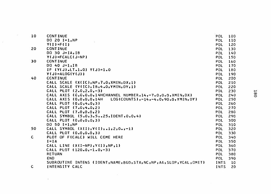
10
20
30
40
50
C
C
CONTINUE DO 20 1=1,NP Y( I) =F (I) CONTINUE DO 30 J=IA,IB Y ( J) =FCALC ( J"'."NP) CONTINUE DO 40 J=l,IB IF (Y(J).LT.1.0J Y(J)=l.O Y(J)=ALOG(Y(J)) CGNTINUE CALL SCALE (X(IC),NP,7.0,XMIN,DX,1) CALL SCALE (Y(IC),18,4.0,YMIN,DY,1) CALL PLOT (2.0,2.0,-3) CALL AXIS (O.o,o.o,14HcHANNEL NUMBER,14,-7.o,o.o,XMIN,DX) CALL AXIS (0.0,0.0,14H LOG(COUNTS),-14,-4.0,90.0,YMIN,DY) CALL PLOT (0.0,4.0,3) CALL PLOT (7.0,4.0,2) CALL PLOT (7.0,0.0,2) CALL SYMBOL (5.0,3.5,.25,IDENT,0.0,4) CALL PLOT co.o,o.o,3) DO 50 1=1,NP CALL SYMBOL (X(I),Y(I),.1,2,0.,-l) CALL PLOT (0.0,0.0,3) PLOT OF F(CALC) Will COME HERE I=IA CALL LINE (X(I-NP),Y(l),NP,1) CALL PLOT (120.0,-1.0,-3) RETURN ENO SUBROUTINE INTENS (IOENT,NAME,BGD,STX,NC,NP,AA,SLOP,YCAL,OMIT) INTENSITY CALC
POL 100 POL 110 POL 120 POL 130 POL 140 POL 150 POL 160 POL 170 POL 180 POL 190 POL 200 POL 210 POL 220 POL 230 POL 240 POL 250 POL 260 POL 270 POL 280 POL 290 POL 300 POL 310 POL 320 POL 330 POL 340 POL 350 POL 360 POL 370 POL 380 POL 390 INTS 10 INTS 20
I-' 00 0

C C C C C C C C C C
C C
10 20
30
C
40
50
BGD IS THE COUNTER BACKGROUND FOR SUBTRACTION STX IS THE NUMBER OF CHANNELS BETWEEN ZERO CHANNEL AND FIRST DATA CHANNEL FOR CALC TAU NC IS THE NUMBER OF COMPONENTS NP IS THE NUMBER OF DATA PTS USED IN CALC TAU FOR COMP AA IS THE COMP INTERCEPT VALUES AT ZERO TIME SLOP IS THE COMPONENT SLOPES YCAL IS THE THEORETICAL VALUES FOR NP DATA POINTS YEXP IS THE EXPERIMENTAL VALUES FOR NEP DATA PTS ON LEFT SIDE OF SPECTRUM FOR DETERMING TOTtL AREA UNDER CURVE DIMENSION NAME(ll), AA(5), SLOP(5), YCAL(512) DIMENSION YEXP(200J, XX(512), AREXP(5), TEN(5), AT(5) INTEGER OMIT READ (5,280) NEP,CONTR NEP IS THE NO. OF ADDITIONAL EXPERIMENTAL GRAPH PTS NEEDED TO CALC COMPONENT INTENSITIES IF CCONTR.NE.0) GO TO 10 READ (5,290) (YEXP(I),I=l,NEP) GO TO 20 READ (5,300) CYEXP(I),I=l,NEP) DO 30 I=l,NEP YEXP(I)=YEXP(I)-BGD CONTINUE IE=I PTST TEST XX(ll=STX DO 40 I=2,NP XX(I)=XX(l-1)+1.0 CONTINUE l=O L=L+l DT=(-SLOP(NC)*XX(l))
INTS 30 I NTS 40 INTS 50 INTS 60 INTS 70 INTS 80 INTS 90 INTS 100 INTS 110 INTS 120 INTS 130 If'ITS 140 INTS 150 INTS 160 INTS 170 INTS 180 HHS 190 INTS 200 INTS 210 INTS 220 INTS 230 INTS 240 INTS 250 INTS 260 INTS 270 INTS 280 INTS 290 INTS 300 INTS 310 INTS 320 INTS 330 INTS 340
..... 00 .....

P=AA(NC)*EXP(DT) INTS 350 PTST=YCAL(L)-P INTS 360 IF (PTST.GT.5.0) GO TO 50 INTS 370 PYS=YCALCL) INTS 380 PXS=XXCL) INTS 390 J=IE+L INTS 400
C CHANGE OF SUBSCRIPTS TO UNIFY THE DATA ORDER INTS 410 DO 60 I=l,L INTS 420 IE=IE+l INTS 430 TEMP=YCALC I) INTS 440 YEXP(IE)=TEMP INTS 450
60 CONTINUE INTS 460 C OUTPUT 1 INTS 47C
WRITE (6,310) IDENT,NAME INTS 480 1--'
WRITE (6,320) NP,NC,BGD,STX ·INTS 490 00 N)
WRITE (6,330) CI,AACIJ,I,SLOP(I),I=l,NC) INTS 500 10 GO TO (80,90,80,90), OMIT INTS 510 80 WRITE (6,340) INTS 520
WRITE (6,350) CI,YEXP(I),I=l,J) INTS 530 C TOTAL AREA UNDER CURVECARSM) INTS 540 C ADJUSTMENT OF THE INDEX J INTS 550 90 ODD=O.O INTS 560
EVEN=O.O INTS 570 KJ=O INTS 580 KI=O INTS 590 NEV=J-1 INTS 600 DO 100 1=2,NEV,2 INTS 610 KJ=KJ+l ' INTS 620 EVEN=EVEN+YEXP(I) INTS 630
100 CONTINUE INTS 640 NOD=J-2 INTS 650 00 110 1=3,NOD,2 INTS 660

KI=Kl+l INTS 670 ODD=OOO+YEXP(I) INTS 680
110 CONTINUE INTS 690 C CALCULATION GF AREA INTS 700
JK=KJ+KI+2 INTS 710 IF (JK-J) 120,140,120 INTS 720
120 J=J-1 INTS 730 DO 130 JK=l,J INTS 740 YEXP(JK)=YEXP(JK+l) HHS 750
130 CONTINUE INTS 760 GO TO 70 INTS 770
140 ARSM=0.33333*1.0*(YEXP(l)+2.0*EVEN+4.0*0DD+YEXP(J)) INTS 780 TA=(-SLOP(NC)*PXS) INTS 790 ARTA=(AA(NC)*EXP(TAJ)/(SLOP(NC)) INTS 800 I-' ARSH=ARSM+ARTA INTS 810 00
WRITE (6,360) ARSM,ARTA,J,PTST,PXS,PYS INTS 820 ~
C SUH OF COMPONENT AREAS(SUM) INT$ 830 SUM=O.O INTS 840 DO 150 I= 1, NC INTS 850 AREXP(l)=AA(l)/(SLOP(I)) INTS 860 SUM=SUM+AREXP (I) INTS 870
150 CONTINUE INTS 880 DO 160 I=l,NC INTS 890 TEN(I)=AREXPCI)/SUM INTS 900
160 CONTINUE INTS 910 WRITE (6,340) INTS 920 WRITE (6,370) SUM INTS 930 WRITE (6,380) CI,TEN(I),I,AREXP(I),I,AA(Il,I=l,NC) INTS 940
C OPTIMIZATION OF ZERO LINE INTS 950 T=O.O INTS 960 AOD=0.1 INTS 970
170 SUM=O.O INTS 980
T=T+AOO HHS 990 IF CT.GT.STX) GO TO 270 INTS1000 DO 180 I=l,NC INTS1010 AT(l)=AACI)*EXP(-SLOP(l)*T) INTS1020 AREXP(l)=AT(I)/SLOP(I) INTS1030 SUM=SUM+AREXPC I J INTS1040
180 CONTINUE I NTS 1050 IF (SUM-ARSM) 190,240,170 INTS1060
190 IF (ABSCCSUM-ARSM)/ARSM).LT.0.01) GO TO 240 INTS1070 T=T-AOO INTS1080 ADO=A00/10.0 INTS1090 IF (AOD.LE.0.0001) GO TO 200 INTS1100 GO TO 170 INTS1110
200 T=O.O INTS1120 I-' 00 SUB=-0.1 INTS1130 Ill-
210 SUM=O.O INTS1140 T=T+SUB INTS1150 DO 220 I=l,NC INTS1160 AT(l)=AA(I)*EXP(-SLOP(l)*T) INTS1170 AREXP(l)=AT(I)/SLOP(l) INTS1180 SUM=SUM+AREXP(I) INTS1190
220 CONTINUE INTS1200 IF CSUM-ARSM) 210,240,230 INTS1210
230 IF CABSCCSUM-ARSM)/ARSM).LT.0.01) GO TO 240 INTS1220 T=T-SUB INTS1230 SUB=SUB/10.0 INTS1240 IF CSUB.LE.0.0001) GO TO 240 INTS1250
240 00 250 I=l,NC INTS1260 TEN(I)=AREXP(I)/SUM INTS1270
250 CONTINUE INTS1280 C OUTPUT 2 INTS1290
WRITE (6,340) INTS1300

260
270 C 280 290 300 310 320 330 340 350
360
370 380
390 400
410
420
WRITE (6,390) SUM,T WRITE (6,400) (I,TEN(IJ,1,AREXP(l),1,AT(I),I=l,NCJ WRITE (6,410) DO 260 I =1,NC TEN(I)=TEN(l)*lOO.O WRITE (6,420) (TEN(l),I=l,NC) RETURN
INTS1310 INTS1320 INTS1330 INTS1340 INTS1350 INTS1360 INTS1370 INTS1380
FOR~AT (215) INTS1390 FORMAT (F6.0,9F7.0) INTS1400 FORMAT (F9.0,7F10.0) INTS1410 FORMAT (1Hl,3X,A4,11A4) INTS1420 FORMAT (//5H NP=,13,SH NC=,I2,6H BGD=,Fl0.5,6H STX=,FS.2//) INTS1430 FORMAT (5X,2HA(,I2,2H)=,F15.5,7H SLOP(,I2,2H)=,Fl2.8) INTS1440 FORMAT (lHO) INTS1450 FORMAT (9H YEXPC,I2,2H)=,Fl5.5,9H YEXP(,12,2H)=,Fl5.5,9H INTS1460
1YEXP(,I2,2H)=,Fl5.5,9H YEXP(,I2,2H)=,Fl5.5) INTS1470 FCRMAT (//10X,5HARSM=,El5.8,7H ARTA=,El5.8,4H J=,I3,7H PTST=,FlINTS1480
10.5,6H PXS=,F8.4,6H PYS=,Fl0.5) INTS1490 FORMAT (15X,4HSUM=,El5.8) INTS1500 FORMAT (10X,2HI(,I2,2H)=,El5.8,5X,8H AREXP(,I2,2H)=,El5.8,5X,4H INTS1510
1A(,I2,2Hl=,F12.5) INTS1520 FORMAT (15X,4HSUM=,E15.8,4H T=,Fl0.5) INTS1530 FORMAT (10X,2HI(,I2,2H)=,El5.8,5X,8H AREXP(,I2,2H)=,El5.8,5X,5H INTS1540
1AT(,I2,2H)=,Fl2.5) INTS1550 FORMAT (////lllH 1ST COMP INTS1560
1 2ND COMP 3RD COMP 4TH COMP 5TH COMP) INTS1570 FORMAT (//5X,15HINTENSITY (%),9X,5Fl6.3) INTS1580 END INTS1590
...... 00 CJ1

The vita has been removed from the scanned document

THE REACT~ON OF ORTHO-POSITRONIUM
WITH NITROAROMATICS
by
William Juul Madia
(ABSTRACT)
A study was made to ascertain the mechanism by which
ortho-positronium reacts with nitroaromatics in solution.
These reactions are two to three orders of magnitude faster
than expected by simple pickoff. Conjugation of the nitro
group with the aromatic ring was found to be a necessary
condition for this behavior. The rate constant for each
of these reactions was measured in suitable solvents over
a wide temperature range, 200-500°K. Distinct departure
from the Arrhenius law was found. In general, the rate
constant increased linearly with increasing temperature up
to a point, and then decreased linearly as the temperature
was raised further. The following mechanism is postulated:
Ps + M PsM ---) M + 2y
Ortho-Positronium reacts with the nitroaromatic, M, to form
a complex in a reversible step, The complex may either
decompose into a positronium atom and nitroaromatic molecule
or it may go on to annihilate the positron. A steady-state

concentration ot the complex is assumed and the observed
rate constant tor the process is
k obs ::::
k + k2 -1
'1'!11~ two limiting cases are: (1) k2 >> k_ 1 causing kobs ~
k 1 . Typical Arrhenius behavior is expected and observed in
thi.s region, and (2) k_ 1 >> k2 causing kobs ~ KEQk2 . In
this region HEQ + Ea(2) <O and the observed rate constant
decreases with increasing temperature. This corresponds
to a stable but temperature sensitive PsM complex.
An approximate molecular orbital study has been made
to study the possible existence of positron and positronium
complexes with a select number of organic molecules. The
CND0/2 approximation is used for all electronic integrals
and for electron positron Coulomb integrals. The core
Hamiltonian matrix elements for the positron were estimated
by combining the Wolfsberg-Helmholtz and Cusachs-Cusachs
approximations. This approach shows that the positron should
become bound to the molecules. Using the same criteria, the
formation of stable positronium complexes is more improbable.
The calculated binding energies are strongly dependent on
the value of the Wolfsberg-Helmholtz proportionality constant
for positrons.