viii

CHAPTER 4

Elliptic PDEs

One of the main advantages of extending the class of solutions of a PDE fromclassical solutions with continuous derivatives to weak solutions with weak deriva-tives is that it is easier to prove the existence of weak solutions. Having estab-lished the existence of weak solutions, one may then study their properties, such asuniqueness and regularity, and perhaps prove under appropriate assumptions thatthe weak solutions are, in fact, classical solutions.

There is often considerable freedom in how one defines a weak solution of aPDE; for example, the function space to which a solution is required to belong isnot given a priori by the PDE itself. Typically, we look for a weak formulation thatreduces to the classical formulation under appropriate smoothness assumptions andwhich is amenable to a mathematical analysis; the notion of solution and the spacesto which solutions belong are dictated by the available estimates and analysis.

4.1. Weak formulation of the Dirichlet problem

Let us consider the Dirichlet problem for the Laplacian with homogeneousboundary conditions on a bounded domain Ω in R

n,

−∆u = f in Ω,(4.1)

u = 0 on ∂Ω.(4.2)

First, suppose that the boundary of Ω is smooth and u, f : Ω → R are smoothfunctions. Multiplying (4.1) by a test function φ, integrating the result over Ω, andusing the divergence theorem, we get

(4.3)

∫

Ω

Du ·Dφdx =

∫

Ω

fφ dx for all φ ∈ C∞c (Ω).

The boundary terms vanish because φ = 0 on the boundary. Conversely, if f andΩ are smooth, then any smooth function u that satisfies (4.3) is a solution of (4.1).

Next, we formulate weaker assumptions under which (4.3) makes sense. Weuse the flexibility of choice to define weak solutions with L2-derivatives that belongto a Hilbert space; this is helpful because Hilbert spaces are easier to work withthan Banach spaces.1 Furthermore, it leads to a variational form of the equationthat is symmetric in the solution u and the test function φ. Our goal of obtaininga symmetric weak formulation also explains why we only integrate by parts oncein (4.3). We briefly discuss some other ways to define weak solutions at the end ofthis section.

1We would need to use Banach spaces to study the solutions of Laplace’s equation whosederivatives lie in Lp for p 6= 2, and we may be forced to use Banach spaces for some PDEs,especially if they are nonlinear.

91

92 4. ELLIPTIC PDES

By the Cauchy-Schwartz inequality, the integral on the left-hand side of (4.3)is finite if Du belongs to L2(Ω), so we suppose that u ∈ H1(Ω). We impose theboundary condition (4.2) in a weak sense by requiring that u ∈ H1

0 (Ω). The left

hand side of (4.3) then extends by continuity to φ ∈ H10 (Ω) = C∞

c (Ω).The right hand side of (4.3) is well-defined for all φ ∈ H1

0 (Ω) if f ∈ L2(Ω), butthis is not the most general f for which it makes sense; we can define the right-handfor any f in the dual space of H1

0 (Ω).

Definition 4.1. The space of bounded linear maps f : H10 (Ω) → R is denoted

by H−1(Ω) = H10 (Ω)

∗, and the action of f ∈ H−1(Ω) on φ ∈ H10 (Ω) by 〈f, φ〉. The

norm of f ∈ H−1(Ω) is given by

‖f‖H−1 = sup

|〈f, φ〉|

‖φ‖H10

: φ ∈ H10 , φ 6= 0

.

A function f ∈ L2(Ω) defines a linear functional Ff ∈ H−1(Ω) by

〈Ff , v〉 =

∫

Ω

fv dx = (f, v)L2 for all v ∈ H10 (Ω).

Here, (·, ·)L2 denotes the standard inner product on L2(Ω). The functional Ff isbounded on H1

0 (Ω) with ‖Ff‖H−1 ≤ ‖f‖L2 since, by the Cauchy-Schwartz inequal-ity,

|〈Ff , v〉| ≤ ‖f‖L2‖v‖L2 ≤ ‖f‖L2‖v‖H10.

We identify Ff with f , and write both simply as f .Such linear functionals are, however, not the only elements of H−1(Ω). As we

will show below, H−1(Ω) may be identified with the space of distributions on Ωthat are sums of first-order distributional derivatives of functions in L2(Ω).

Thus, after identifying functions with regular distributions, we have the follow-ing triple of Hilbert spaces

H10 (Ω) → L2(Ω) → H−1(Ω), H−1(Ω) = H1

0 (Ω)∗.

Moreover, if f ∈ L2(Ω) ⊂ H−1(Ω) and u ∈ H10 (Ω), then

〈f, u〉 = (f, u)L2 ,

so the duality pairing coincides with the L2-inner product when both are defined.This discussion motivates the following definition.

Definition 4.2. Let Ω be an open set in Rn and f ∈ H−1(Ω). A function

u : Ω → R is a weak solution of (4.1)–(4.2) if: (a) u ∈ H10 (Ω); (b)

(4.4)

∫

Ω

Du ·Dφdx = 〈f, φ〉 for all φ ∈ H10 (Ω).

Here, strictly speaking, ‘function’ means an equivalence class of functions withrespect to pointwise a.e. equality.

We have assumed homogeneous boundary conditions to simplify the discussion.If Ω is smooth and g : ∂Ω → R is a function on the boundary that is in the rangeof the trace map T : H1(Ω) → L2(∂Ω), say g = Tw, then we obtain a weakformulation of the nonhomogeneous Dirichet problem

−∆u = f in Ω,

u = g on ∂Ω,

4.2. VARIATIONAL FORMULATION 93

by replacing (a) in Definition 4.2 with the condition that u − w ∈ H10 (Ω). The

definition is otherwise the same. The range of the trace map on H1(Ω) for a smoothdomain Ω is the fractional-order Sobolev space H1/2(∂Ω); thus if the boundarydata g is so rough that g /∈ H1/2(∂Ω), then there is no solution u ∈ H1(Ω) of thenonhomogeneous BVP.

Finally, we comment on some other ways to define weak solutions of Poisson’sequation. If we integrate by parts again in (4.3), we find that every smooth solutionu of (4.1) satisfies

(4.5) −

∫

Ω

u∆φdx =

∫

Ω

fφ dx for all φ ∈ C∞c (Ω).

This condition makes sense without any differentiability assumptions on u, andwe can define a locally integrable function u ∈ L1

loc(Ω) to be a weak solution of−∆u = f for f ∈ L1

loc(Ω) if it satisfies (4.5). One problem with using this definitionis that general functions u ∈ Lp(Ω) do not have enough regularity to make sense oftheir boundary values on ∂Ω.2

More generally, we can define distributional solutions T ∈ D′(Ω) of Poisson’sequation −∆T = f with f ∈ D′(Ω) by

(4.6) − 〈T,∆φ〉 = 〈f, φ〉 for all φ ∈ C∞c (Ω).

While these definitions appear more general, because of elliptic regularity they turnout not to extend the class of variational solutions we consider here if f ∈ H−1(Ω),and we will not use them below.

4.2. Variational formulation

Definition 4.2 of a weak solution in is closely connected with the variationalformulation of the Dirichlet problem for Poisson’s equation. To explain this con-nection, we first summarize some definitions of the differentiability of functionals(scalar-valued functions) acting on a Banach space.

Definition 4.3. A functional J : X → R on a Banach space X is differentiableat x ∈ X if there is a bounded linear functional A : X → R such that

limh→0

|J(x+ h)− J(x)−Ah|

‖h‖X= 0.

If A exists, then it is unique, and it is called the derivative, or differential, of J atx, denoted DJ(x) = A.

This definition expresses the basic idea of a differentiable function as one whichcan be approximated locally by a linear map. If J is differentiable at every pointof X , then DJ : X → X∗ maps x ∈ X to the linear functional DJ(x) ∈ X∗ thatapproximates J near x.

2For example, if Ω is bounded and ∂Ω is smooth, then pointwise evaluation φ 7→ φ|∂Ω on

C(Ω) extends to a bounded, linear trace map T : Hs(Ω) → Hs−1/2(Ω) if s > 1/2 but notif s ≤ 1/2. In particular, there is no sensible definition of the boundary values of a generalfunction u ∈ L2(Ω). We remark, however, that if u ∈ L2(Ω) is a weak solution of −∆u = fwhere f ∈ L2(Ω), then elliptic regularity implies that u ∈ H2(Ω), so it does have a well-defined

boundary value u|∂Ω ∈ H3/2(∂Ω); on the other hand, if f ∈ H−2(Ω), then u ∈ L2(Ω) and we

cannot make sense of u|∂Ω.

94 4. ELLIPTIC PDES

A weaker notion of differentiability (even for functions J : R2 → R — see

Example 4.4) is the existence of directional derivatives

δJ(x;h) = limǫ→0

[

J(x + ǫh)− J(x)

ǫ

]

=d

dǫJ(x+ ǫh)

∣

∣

∣

∣

ǫ=0

.

If the directional derivative at x exists for every h ∈ X and is a bounded linearfunctional on h, then δJ(x;h) = δJ(x)h where δJ(x) ∈ X∗. We call δJ(x) theGateaux derivative of J at x. The derivativeDJ is then called the Frechet derivativeto distinguish it from the directional or Gateaux derivative. If J is differentiableat x, then it is Gateaux-differentiable at x and DJ(x) = δJ(x), but the converse isnot true.

Example 4.4. Define f : R2 → R by f(0, 0) = 0 and

f(x, y) =

(

xy2

x2 + y4

)2

if (x, y) 6= (0, 0).

Then f is Gateaux-differentiable at 0, with δf(0) = 0, but f is not Frechet-differentiable at 0.

If J : X → R attains a local minimum at x ∈ X and J is differentiable at x,then for every h ∈ X the function Jx;h : R → R defined by Jx;h(t) = J(x + th) isdifferentiable at t = 0 and attains a minimum at t = 0. It follows that

dJx;hdt

(0) = δJ(x;h) = 0 for every h ∈ X.

Hence DJ(x) = 0. Thus, just as in multivariable calculus, an extreme point of adifferentiable functional is a critical point where the derivative is zero.

Given f ∈ H−1(Ω), define a quadratic functional J : H10 (Ω) → R by

(4.7) J(u) =1

2

∫

Ω

|Du|2dx− 〈f, u〉.

Clearly, J is well-defined.

Proposition 4.5. The functional J : H10 (Ω) → R in (4.7) is differentiable. Its

derivative DJ(u) : H10 (Ω) → R at u ∈ H1

0 (Ω) is given by

DJ(u)h =

∫

Ω

Du ·Dhdx− 〈f, h〉 for h ∈ H10 (Ω).

Proof. Given u ∈ H10 (Ω), define the linear map A : H1

0 (Ω) → R by

Ah =

∫

Ω

Du ·Dhdx− 〈f, h〉.

Then A is bounded, with ‖A‖ ≤ ‖Du‖L2 + ‖f‖H−1 , since

|Ah| ≤ ‖Du‖L2‖Dh‖L2 + ‖f‖H−1‖h‖H10≤ (‖Du‖L2 + ‖f‖H−1) ‖h‖H1

0.

For h ∈ H10 (Ω), we have

J(u+ h)− J(u)−Ah =1

2

∫

Ω

|Dh|2dx.

It follows that

|J(u+ h)− J(u)−Ah| ≤1

2‖h‖

2H1

0,

4.3. THE SPACE H−1(Ω) 95

and therefore

limh→0

|J(u+ h)− J(u)−Ah|

‖h‖H10

= 0,

which proves that J is differentiable on H10 (Ω) with DJ(u) = A.

Note that DJ(u) = 0 if and only if u is a weak solution of Poisson’s equationin the sense of Definition 4.2. Thus, we have the following result.

Corollary 4.6. If J : H10 (Ω) → R defined in (4.7) attains a minimum at

u ∈ H10 (Ω), then u is a weak solution of −∆u = f in the sense of Definition 4.2.

In the direct method of the calculus of variations, we prove the existence of aminimizer of J by showing that a minimizing sequence un converges in a suitablesense to a minimizer u. This minimizer is then a weak solution of (4.1)–(4.2). Wewill not follow this method here, and instead establish the existence of a weaksolution by use of the Riesz representation theorem. The Riesz representationtheorem is, however, typically proved by a similar argument to the one used in thedirect method of the calculus of variations, so in essence the proofs are equivalent.

4.3. The space H−1(Ω)

The negative order Sobolev space H−1(Ω) can be described as a space of dis-tributions on Ω.

Theorem 4.7. The space H−1(Ω) consists of all distributions f ∈ D′(Ω) of theform

(4.8) f = f0 +

n∑

i=1

∂ifi where f0, fi ∈ L2(Ω).

These distributions extend uniquely by continuity from D(Ω) to bounded linear func-tionals on H1

0 (Ω). Moreover,

(4.9) ‖f‖H−1(Ω) = inf

(

n∑

i=0

∫

Ω

f2i dx

)1/2

: such that f0, fi satisfy (4.8)

.

Proof. First suppose that f ∈ H−1(Ω). By the Riesz representation theoremthere is a function g ∈ H1

0 (Ω) such that

(4.10) 〈f, φ〉 = (g, φ)H10

for all φ ∈ H10 (Ω).

Here, (·, ·)H10denotes the standard inner product on H1

0 (Ω),

(u, v)H10=

∫

Ω

(uv +Du ·Dv) dx.

Identifying a function g ∈ L2(Ω) with its corresponding regular distribution, re-stricting f to φ ∈ D(Ω) ⊂ H1

0 (Ω), and using the definition of the distributional

96 4. ELLIPTIC PDES

derivative, we have

〈f, φ〉 =

∫

Ω

gφ dx+

n∑

i=1

∫

Ω

∂ig ∂iφdx

= 〈g, φ〉+

n∑

i=1

〈∂ig, ∂iφ〉

=

⟨

g −

n∑

i=1

∂igi, φ

⟩

for all φ ∈ D(Ω),

where gi = ∂ig ∈ L2(Ω). Thus the restriction of every f ∈ H−1(Ω) from H10 (Ω) to

D(Ω) is a distribution

f = g −

n∑

i=1

∂igi

of the form (4.8). Also note that taking φ = g in (4.10), we get 〈f, g〉 = ‖g‖2H1

0

,

which implies that

‖f‖H−1 ≥ ‖g‖H10=

(

∫

Ω

g2 dx+n∑

i=1

∫

Ω

g2i dx

)1/2

,

which proves inequality in one direction of (4.9).Conversely, suppose that f ∈ D′(Ω) is a distribution of the form (4.8). Then,

using the definition of the distributional derivative, we have for any φ ∈ D(Ω) that

〈f, φ〉 = 〈f0, φ〉 +

n∑

i=1

〈∂ifi, φ〉 = 〈f0, φ〉 −

n∑

i=1

〈fi, ∂iφ〉.

Use of the Cauchy-Schwartz inequality gives

|〈f, φ〉| ≤

(

〈f0, φ〉2 +

n∑

i=1

〈fi, ∂iφ〉2

)1/2

.

Moreover, since the fi are regular distributions belonging to L2(Ω)

|〈fi, ∂iφ〉| =

∣

∣

∣

∣

∫

Ω

fi∂iφdx

∣

∣

∣

∣

≤

(∫

Ω

f2i dx

)1/2(∫

Ω

∂iφ2 dx

)1/2

,

so

|〈f, φ〉| ≤

[

(∫

Ω

f20 dx

)(∫

Ω

φ2 dx

)

+n∑

i=1

(∫

Ω

f2i dx

)(∫

Ω

∂iφ2 dx

)

]1/2

,

and

|〈f, φ〉| ≤

(

∫

Ω

f20 dx+

n∑

i=1

∫

Ω

f2i dx

)1/2(∫

Ω

φ2 +

∫

Ω

∂iφ2 dx

)1/2

≤

(

n∑

i=0

∫

Ω

f2i dx

)1/2

‖φ‖H10

4.3. THE SPACE H−1(Ω) 97

Thus the distribution f : D(Ω) → R is bounded with respect to the H10 (Ω)-norm

on the dense subset D(Ω). It therefore extends in a unique way to a bounded linearfunctional on H1

0 (Ω), which we still denote by f . Moreover,

‖f‖H−1 ≤

(

n∑

i=0

∫

Ω

f2i dx

)1/2

,

which proves inequality in the other direction of (4.9).

The dual space of H1(Ω) cannot be identified with a space of distributions on Ωbecause D(Ω) is not a dense subspace. Any linear functional f ∈ H1(Ω)∗ defines adistribution by restriction to D(Ω), but the same distribution arises from differentlinear functionals. Conversely, any distribution T ∈ D′(Ω) that is bounded withrespect to the H1-norm extends uniquely to a bounded linear functional on H1

0 , butthe extension of the functional to the orthogonal complement (H1

0 )⊥ in H1 is ar-

bitrary (subject to maintaining its boundedness). Roughly speaking, distributionsare defined on functions whose boundary values or trace is zero, but general linearfunctionals on H1 depend on the trace of the function on the boundary ∂Ω.

Example 4.8. The one-dimensional Sobolev space H1(0, 1) is embedded in thespace C([0, 1]) of continuous functions, since p > n for p = 2 and n = 1. In fact,according to the Sobolev embedding theorem H1(0, 1) → C0,1/2([0, 1]), as can beseen directly from the Cauchy-Schwartz inequality:

|f(x)− f(y)| ≤

∫ x

y

|f ′(t)| dt

≤

(∫ x

y

1 dt

)1/2(∫ x

y

|f ′(t)|2dt

)1/2

≤

(∫ 1

0

|f ′(t)|2dt

)1/2

|x− y|1/2 .

As usual, we identify an element of H1(0, 1) with its continuous representative inC([0, 1]). By the trace theorem,

H10 (0, 1) =

u ∈ H1(0, 1) : u(0) = 0, u(1) = 0

.

The orthogonal complement is

H10 (0, 1)

⊥ =

u ∈ H1(0, 1) : such that (u, v)H1 = 0 for every v ∈ H10 (0, 1)

.

This condition implies that u ∈ H10 (0, 1)

⊥ if and only if∫ 1

0

(uv + u′v′) dx = 0 for all v ∈ H10 (0, 1),

which means that u is a weak solution of the ODE

−u′′ + u = 0.

It follows that u(x) = c1ex + c2e

−x, so

H1(0, 1) = H10 (0, 1)⊕ E

where E is the two dimensional subspace of H1(0, 1) spanned by the orthogonalvectors ex, e−x. Thus,

H1(0, 1)∗ = H−1(0, 1)⊕ E∗.

98 4. ELLIPTIC PDES

If f ∈ H1(0, 1)∗ and u = u0 + c1ex + c2e

−x where u0 ∈ H10 (0, 1), then

〈f, u〉 = 〈f0, u0〉+ a1c1 + a2c2

where f0 ∈ H−1(0, 1) is the restriction of f to H10 (0, 1) and

a1 = 〈f, ex〉, a2 = 〈f, e−x〉.

The constants a1, a2 determine how the functional f ∈ H1(0, 1)∗ acts on theboundary values u(0), u(1) of a function u ∈ H1(0, 1).

4.4. The Poincare inequality for H10 (Ω)

We cannot, in general, estimate a norm of a function in terms of a norm of itsderivative since constant functions have zero derivative. Such estimates are possibleif we add an additional condition that eliminates non-zero constant functions. Forexample, we can require that the function vanishes on the boundary of a domain, orthat it has zero mean. We typically also need some sort of boundedness conditionon the domain of the function, since even if a function vanishes at some point wecannot expect to estimate the size of a function over arbitrarily large distances bythe size of its derivative. The resulting inequalities are called Poincare inequalities.

The inequality we prove here is a basic example of a Poincare inequality. Wesay that an open set Ω in R

n is bounded in some direction if there is a unit vectore ∈ R

n and constants a, b such that a < x · e < b for all x ∈ Ω.

Theorem 4.9. Suppose that Ω is an open set in Rn that is bounded is some

direction. Then there is a constant C such that

(4.11)

∫

Ω

u2 dx ≤ C

∫

Ω

|Du|2dx for all u ∈ H1

0 (Ω).

Proof. Since C∞c (Ω) is dense in H1

0 (Ω), it is sufficient to prove the inequalityfor u ∈ C∞

c (Ω). The inequality is invariant under rotations and translations, sowe can assume without loss of generality that the domain is bounded in the xn-direction and lies between 0 < xn < a.

Writing x = (x′, xn) where x′ = (x1, . . . , , xn−1), we have

|u(x′, xn)| =

∣

∣

∣

∣

∫ xn

0

∂nu(x′, t) dt

∣

∣

∣

∣

≤

∫ a

0

|∂nu(x′, t)| dt.

The Cauchy-Schwartz inequality implies that∫ a

0

|∂nu(x′, t)| dt =

∫ a

0

1 · |∂nu(x′, t)| dt ≤ a1/2

(∫ a

0

|∂nu(x′, t)|

2dt

)1/2

.

Hence,

|u(x′, xn)|2≤ a

∫ a

0

|∂nu(x′, t)|

2dt.

Integrating this inequality with respect to xn, we get∫ a

0

|u(x′, xn)|2dxn ≤ a2

∫ a

0

|∂nu(x′, t)|

2dt.

A further integration with respect to x′ gives∫

Ω

|u(x)|2dx ≤ a2

∫

Ω

|∂nu(x)|2dx.

Since |∂nu| ≤ |Du|, the result follows with C = a2.

4.5. EXISTENCE OF WEAK SOLUTIONS OF THE DIRICHLET PROBLEM 99

This inequality implies that we may use as an equivalent inner-product onH1

0 an expression that involves only the derivatives of the functions and not thefunctions themselves.

Corollary 4.10. If Ω is an open set that is bounded in some direction, thenH1

0 (Ω) equipped with the inner product

(4.12) (u, v)0 =

∫

Ω

Du ·Dv dx

is a Hilbert space, and the corresponding norm is equivalent to the standard normon H1

0 (Ω).

Proof. We denote the norm associated with the inner-product (4.12) by

‖u‖0 =

(∫

Ω

|Du|2 dx

)1/2

,

and the standard norm and inner product by

‖u‖1 =

(∫

Ω

[

u2 + |Du|2]

dx

)1/2

,

(u, v)1 =

∫

Ω

(uv +Du ·Dv) dx.

(4.13)

Then, using the Poincare inequality (4.11), we have

‖u‖0 ≤ ‖u‖1 ≤ (C + 1)1/2‖u‖0.

Thus, the two norms are equivalent; in particular, (H10 , (·, ·)0) is complete since

(H10 , (·, ·)1) is complete, so it is a Hilbert space with respect to the inner product

(4.12).

4.5. Existence of weak solutions of the Dirichlet problem

With these preparations, the existence of weak solutions is an immediate con-sequence of the Riesz representation theorem.

Theorem 4.11. Suppose that Ω is an open set in Rn that is bounded in some

direction and f ∈ H−1(Ω). Then there is a unique weak solution u ∈ H10 (Ω) of

−∆u = f in the sense of Definition 4.2.

Proof. We equip H10 (Ω) with the inner product (4.12). Then, since Ω is

bounded in some direction, the resulting norm is equivalent to the standard norm,and f is a bounded linear functional on

(

H10 (Ω), (, )0

)

. By the Riesz representation

theorem, there exists a unique u ∈ H10 (Ω) such that

(u, φ)0 = 〈f, φ〉 for all φ ∈ H10 (Ω),

which is equivalent to the condition that u is a weak solution.

The same approach works for other symmetric linear elliptic PDEs. Let us givesome examples.

Example 4.12. Consider the Dirichlet problem

−∆u+ u = f in Ω,

u = 0 on ∂Ω.

100 4. ELLIPTIC PDES

Then u ∈ H10 (Ω) is a weak solution if∫

Ω

(Du ·Dφ+ uφ) dx = 〈f, φ〉 for all φ ∈ H10 (Ω).

This is equivalent to the condition that

(u, φ)1 = 〈f, φ〉 for all φ ∈ H10 (Ω).

where (·, ·)1 is the standard inner product on H10 (Ω) given in (4.13). Thus, the

Riesz representation theorem implies the existence of a unique weak solution.Note that in this example and the next, we do not use the Poincare inequality, so

the result applies to arbitrary open sets, including Ω = Rn. In that case, H1

0 (Rn) =

H1(Rn), and we get a unique solution u ∈ H1(Rn) of −∆u + u = f for everyf ∈ H−1(Rn). Moreover, using the standard norms, we have ‖u‖H1 = ‖f‖H−1 .Thus the operator −∆+ I is an isometry of H1(Rn) onto H−1(Rn).

Example 4.13. As a slight generalization of the previous example, supposethat µ > 0. A function u ∈ H1

0 (Ω) is a weak solution of

−∆u+ µu = f in Ω,

u = 0 on ∂Ω.(4.14)

if (u, φ)µ = 〈f, φ〉 for all φ ∈ H10 (Ω) where

(u, v)µ =

∫

Ω

(µuv +Du ·Dv) dx

The norm ‖ · ‖µ associated with this inner product is equivalent to the standardone, since

1

C‖u‖2µ ≤ ‖u‖21 ≤ C‖u‖2µ

where C = maxµ, 1/µ. We therefore again get the existence of a unique weaksolution from the Riesz representation theorem.

Example 4.14. Consider the last example for µ < 0. If we have a Poincareinequality ‖u‖L2 ≤ C‖Du‖L2 for Ω, which is the case if Ω is bounded in somedirection, then

(u, u)µ =

∫

Ω

(

µu2 + |Du|2)

dx ≥ (1− C|µ|)

∫

Ω

|Du|2dx.

Thus ‖u‖µ defines a norm on H10 (Ω) that is equivalent to the standard norm if

−1/C < µ < 0, and we get a unique weak solution in this case also, provided that|µ| is sufficiently small.

For bounded domains, the Dirichlet Laplacian has an infinite sequence of realeigenvalues λn : n ∈ N such that there exists a nonzero solution u ∈ H1

0 (Ω) of−∆u = λnu. The best constant in the Poincare inequality can be shown to be theminimum eigenvalue λ1, and this method does not work if µ ≤ −λ1. For µ = −λn,a weak solution of (4.14) does not exist for every f ∈ H−1(Ω), and if one does existit is not unique since we can add to it an arbitrary eigenfunction. Thus, not onlydoes the method fail, but the conclusion of Theorem 4.11 may be false.

4.6. GENERAL LINEAR, SECOND ORDER ELLIPTIC PDES 101

Example 4.15. Consider the second order PDE

−n∑

i,j=1

∂i (aij∂ju) = f in Ω,

u = 0 on ∂Ω

(4.15)

where the coefficient functions aij : Ω → R are symmetric (aij = aji), bounded,and satisfy the uniform ellipticity condition that for some θ > 0

n∑

i,j=1

aij(x)ξiξj ≥ θ|ξ|2 for all x ∈ Ω and all ξ ∈ Rn.

Also, assume that Ω is bounded in some direction. Then a weak formulation of(4.15) is that u ∈ H1

0 (Ω) and

a(u, φ) = 〈f, φ〉 for all φ ∈ H10 (Ω),

where the symmetric bilinear form a : H10 (Ω)×H1

0 (Ω) → R is defined by

a(u, v) =

n∑

i,j=1

∫

Ω

aij∂iu∂jv dx.

The boundedness of aij , the uniform ellipticity condition, and the Poincare inequal-ity imply that a defines an inner product on H1

0 which is equivalent to the standardone. An application of the Riesz representation theorem for the bounded linearfunctionals f on the Hilbert space (H1

0 , a) then implies the existence of a uniqueweak solution. We discuss a generalization of this example in greater detail in thenext section.

4.6. General linear, second order elliptic PDEs

Consider PDEs of the formLu = f

where L is a linear differential operator of the form

(4.16) Lu = −

n∑

i,j=1

∂i (aij∂ju) +

n∑

i=1

∂i (biu) + cu,

acting on functions u : Ω → R where Ω is an open set in Rn. A physical interpre-

tation of such PDEs is described briefly in Section 4.A.We assume that the given coefficients functions aij , bi, c : Ω → R satisfy

(4.17) aij , bi, c ∈ L∞(Ω), aij = aji.

The operator L is elliptic if the matrix (aij) is positive definite. We will assumethe stronger condition of uniformly ellipticity given in the next definition.

Definition 4.16. The operator L in (4.16) is uniformly elliptic on Ω if thereexists a constant θ > 0 such that

(4.18)

n∑

i,j=1

aij(x)ξiξj ≥ θ|ξ|2

for x almost everywhere in Ω and every ξ ∈ Rn.

This uniform ellipticity condition allows us to estimate the integral of |Du|2 interms of the integral of

∑

aij∂iu∂ju.

102 4. ELLIPTIC PDES

Example 4.17. The Laplacian operator L = −∆ is uniformly elliptic on anyopen set, with θ = 1.

Example 4.18. The Tricomi operator

L = y∂2x + ∂2y

is elliptic in y > 0 and hyperbolic in y < 0. For any 0 < ǫ < 1, L is uniformlyelliptic in the strip (x, y) : ǫ < y < 1, with θ = ǫ, but it is not uniformly ellipticin (x, y) : 0 < y < 1.

For µ ∈ R, we consider the Dirichlet problem for L+ µI,

Lu+ µu = f in Ω,

u = 0 on ∂Ω.(4.19)

We motivate the definition of a weak solution of (4.19) in a similar way to themotivation for the Laplacian: multiply the PDE by a test function φ ∈ C∞

c (Ω),integrate over Ω, and use integration by parts, assuming that all functions and thedomain are smooth. Note that

∫

Ω

∂i(biu)φdx = −

∫

Ω

biu∂iφdx.

This leads to the condition that u ∈ H10 (Ω) is a weak solution of (4.19) with L

given by (4.16) if

∫

Ω

n∑

i,j=1

aij∂iu∂jφ−

n∑

i=1

biu∂iφ+ cuφ

dx + µ

∫

Ω

uφdx = 〈f, φ〉

for all φ ∈ H10 (Ω).

To write this condition more concisely, we define a bilinear form

a : H10 (Ω)×H1

0 (Ω) → R

by

(4.20) a(u, v) =

∫

Ω

n∑

i,j=1

aij∂iu∂jv −

n∑

i

biu∂iv + cuv

dx.

This form is well-defined and bounded on H10 (Ω), as we check explicitly below. We

denote the L2-inner product by

(u, v)L2 =

∫

Ω

uv dx.

Definition 4.19. Suppose that Ω is an open set in Rn, f ∈ H−1(Ω), and L is

a differential operator (4.16) whose coefficients satisfy (4.17). Then u : Ω → R is aweak solution of (4.19) if: (a) u ∈ H1

0 (Ω); (b)

a(u, φ) + µ(u, φ)L2 = 〈f, φ〉 for all φ ∈ H10 (Ω).

The form a in (4.20) is not symmetric unless bi = 0. We have

a(v, u) = a∗(u, v)

4.7. THE LAX-MILGRAM THEOREM AND GENERAL ELLIPTIC PDES 103

where

(4.21) a∗(u, v) =

∫

Ω

n∑

i,j=1

aij∂iu∂jv +

n∑

i

bi(∂iu)v + cuv

dx

is the bilinear form associated with the formal adjoint L∗ of L,

(4.22) L∗u = −

n∑

i,j=1

∂i (aij∂ju)−

n∑

i=1

bi∂iu+ cu.

The proof of the existence of a weak solution of (4.19) is similar to the prooffor the Dirichlet Laplacian, with one exception. If L is not symmetric, we cannotuse a to define an equivalent inner product on H1

0 (Ω) and appeal to the Rieszrepresentation theorem. Instead we use a result due to Lax and Milgram whichapplies to non-symmetric bilinear forms.3

4.7. The Lax-Milgram theorem and general elliptic PDEs

We begin by stating the Lax-Milgram theorem for a bilinear form on a Hilbertspace. Afterwards, we verify its hypotheses for the bilinear form associated witha general second-order uniformly elliptic PDE and use it to prove the existence ofweak solutions.

Theorem 4.20. Let H be a Hilbert space with inner-product (·, ·) : H×H → R,and let a : H×H → R be a bilinear form on H. Assume that there exist constantsC1, C2 > 0 such that

C1‖u‖2 ≤ a(u, u), |a(u, v)| ≤ C2‖u‖ ‖v‖ for all u, v ∈ H.

Then for every bounded linear functional f : H → R, there exists a unique u ∈ Hsuch that

〈f, v〉 = a(u, v) for all v ∈ H.

For the proof, see [9]. The verification of the hypotheses for (4.20) depends onthe following energy estimates.

Theorem 4.21. Let a be the bilinear form on H10 (Ω) defined in (4.20), where

the coefficients satisfy (4.17) and the uniform ellipticity condition (4.18) with con-stant θ. Then there exist constants C1, C2 > 0 and γ ∈ R such that for allu, v ∈ H1

0 (Ω)

C1‖u‖2H1

0

≤ a(u, u) + γ‖u‖2L2(4.23)

|a(u, v)| ≤ C2 ‖u‖H10‖v‖H1

0,(4.24)

If b = 0, we may take γ = θ − c0 where c0 = infΩ c, and if b 6= 0, we may take

γ =1

2θ

n∑

i=1

‖bi‖2L∞ +

θ

2− c0.

3The story behind this result — the story might be completely true or completely false —

is that Lax and Milgram attended a seminar where the speaker proved existence for a symmetricPDE by use of the Riesz representation theorem, and one of them asked the other if symmetrywas required; in half an hour, they convinced themselves that is wasn’t, giving birth to the Lax-Milgram “lemma.”

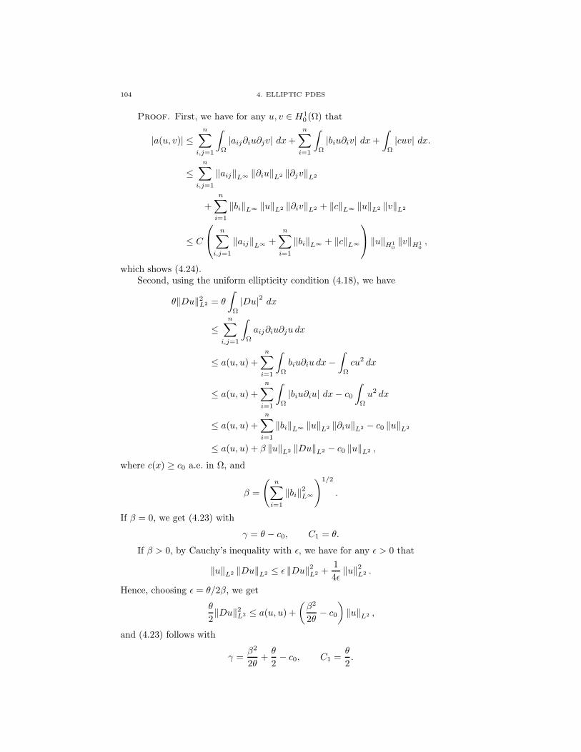
104 4. ELLIPTIC PDES

Proof. First, we have for any u, v ∈ H10 (Ω) that

|a(u, v)| ≤

n∑

i,j=1

∫

Ω

|aij∂iu∂jv| dx+

n∑

i=1

∫

Ω

|biu∂iv| dx+

∫

Ω

|cuv| dx.

≤

n∑

i,j=1

‖aij‖L∞ ‖∂iu‖L2 ‖∂jv‖L2

+

n∑

i=1

‖bi‖L∞ ‖u‖L2 ‖∂iv‖L2 + ‖c‖L∞ ‖u‖L2 ‖v‖L2

≤ C

n∑

i,j=1

‖aij‖L∞ +

n∑

i=1

‖bi‖L∞ + ‖c‖L∞

‖u‖H10‖v‖H1

0,

which shows (4.24).Second, using the uniform ellipticity condition (4.18), we have

θ‖Du‖2L2 = θ

∫

Ω

|Du|2dx

≤

n∑

i,j=1

∫

Ω

aij∂iu∂ju dx

≤ a(u, u) +

n∑

i=1

∫

Ω

biu∂iu dx−

∫

Ω

cu2 dx

≤ a(u, u) +

n∑

i=1

∫

Ω

|biu∂iu| dx− c0

∫

Ω

u2 dx

≤ a(u, u) +

n∑

i=1

‖bi‖L∞ ‖u‖L2 ‖∂iu‖L2 − c0 ‖u‖L2

≤ a(u, u) + β ‖u‖L2 ‖Du‖L2 − c0 ‖u‖L2 ,

where c(x) ≥ c0 a.e. in Ω, and

β =

(

n∑

i=1

‖bi‖2L∞

)1/2

.

If β = 0, we get (4.23) with

γ = θ − c0, C1 = θ.

If β > 0, by Cauchy’s inequality with ǫ, we have for any ǫ > 0 that

‖u‖L2 ‖Du‖L2 ≤ ǫ ‖Du‖2L2 +

1

4ǫ‖u‖

2L2 .

Hence, choosing ǫ = θ/2β, we get

θ

2‖Du‖2L2 ≤ a(u, u) +

(

β2

2θ− c0

)

‖u‖L2 ,

and (4.23) follows with

γ =β2

2θ+θ

2− c0, C1 =

θ

2.

4.8. COMPACTNESS OF THE RESOLVENT 105

Equation (4.23) is called Garding’s inequality; this estimate of the H10 -norm

of u in terms of a(u, u), using the uniform ellipticity of L, is the crucial energyestimate. Equation (4.24) states that the bilinear form a is bounded on H1

0 . Theexpression for γ in this Theorem is not necessarily sharp. For example, as in thecase of the Laplacian, the use of Poincare’s inequality gives smaller values of γ forbounded domains.

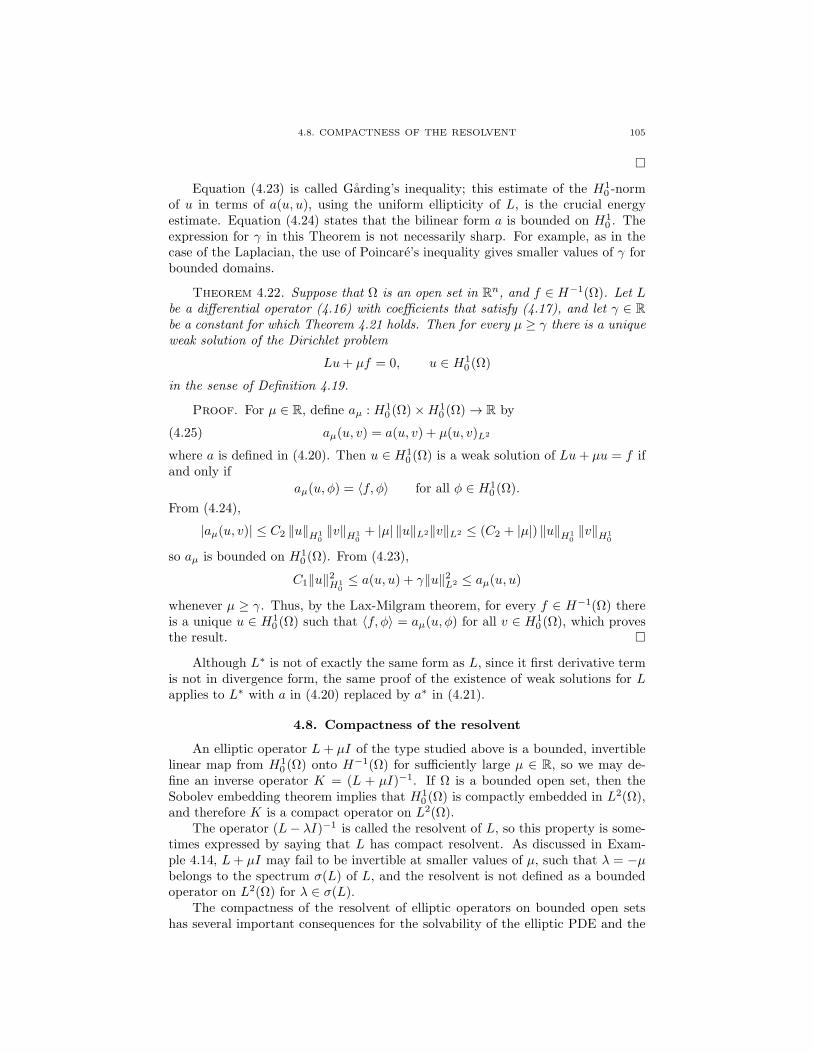
Theorem 4.22. Suppose that Ω is an open set in Rn, and f ∈ H−1(Ω). Let L

be a differential operator (4.16) with coefficients that satisfy (4.17), and let γ ∈ R

be a constant for which Theorem 4.21 holds. Then for every µ ≥ γ there is a uniqueweak solution of the Dirichlet problem

Lu+ µf = 0, u ∈ H10 (Ω)

in the sense of Definition 4.19.

Proof. For µ ∈ R, define aµ : H10 (Ω)×H1

0 (Ω) → R by

(4.25) aµ(u, v) = a(u, v) + µ(u, v)L2

where a is defined in (4.20). Then u ∈ H10 (Ω) is a weak solution of Lu+ µu = f if

and only if

aµ(u, φ) = 〈f, φ〉 for all φ ∈ H10 (Ω).

From (4.24),

|aµ(u, v)| ≤ C2 ‖u‖H10‖v‖H1

0+ |µ| ‖u‖L2‖v‖L2 ≤ (C2 + |µ|) ‖u‖H1

0‖v‖H1

0

so aµ is bounded on H10 (Ω). From (4.23),

C1‖u‖2H1

0

≤ a(u, u) + γ‖u‖2L2 ≤ aµ(u, u)

whenever µ ≥ γ. Thus, by the Lax-Milgram theorem, for every f ∈ H−1(Ω) thereis a unique u ∈ H1

0 (Ω) such that 〈f, φ〉 = aµ(u, φ) for all v ∈ H10 (Ω), which proves

the result.

Although L∗ is not of exactly the same form as L, since it first derivative termis not in divergence form, the same proof of the existence of weak solutions for Lapplies to L∗ with a in (4.20) replaced by a∗ in (4.21).

4.8. Compactness of the resolvent

An elliptic operator L + µI of the type studied above is a bounded, invertiblelinear map from H1

0 (Ω) onto H−1(Ω) for sufficiently large µ ∈ R, so we may de-fine an inverse operator K = (L + µI)−1. If Ω is a bounded open set, then theSobolev embedding theorem implies that H1

0 (Ω) is compactly embedded in L2(Ω),and therefore K is a compact operator on L2(Ω).

The operator (L− λI)−1 is called the resolvent of L, so this property is some-times expressed by saying that L has compact resolvent. As discussed in Exam-ple 4.14, L+ µI may fail to be invertible at smaller values of µ, such that λ = −µbelongs to the spectrum σ(L) of L, and the resolvent is not defined as a boundedoperator on L2(Ω) for λ ∈ σ(L).

The compactness of the resolvent of elliptic operators on bounded open setshas several important consequences for the solvability of the elliptic PDE and the

106 4. ELLIPTIC PDES

spectrum of the elliptic operator. Before describing some of these, we discuss theresolvent in more detail.

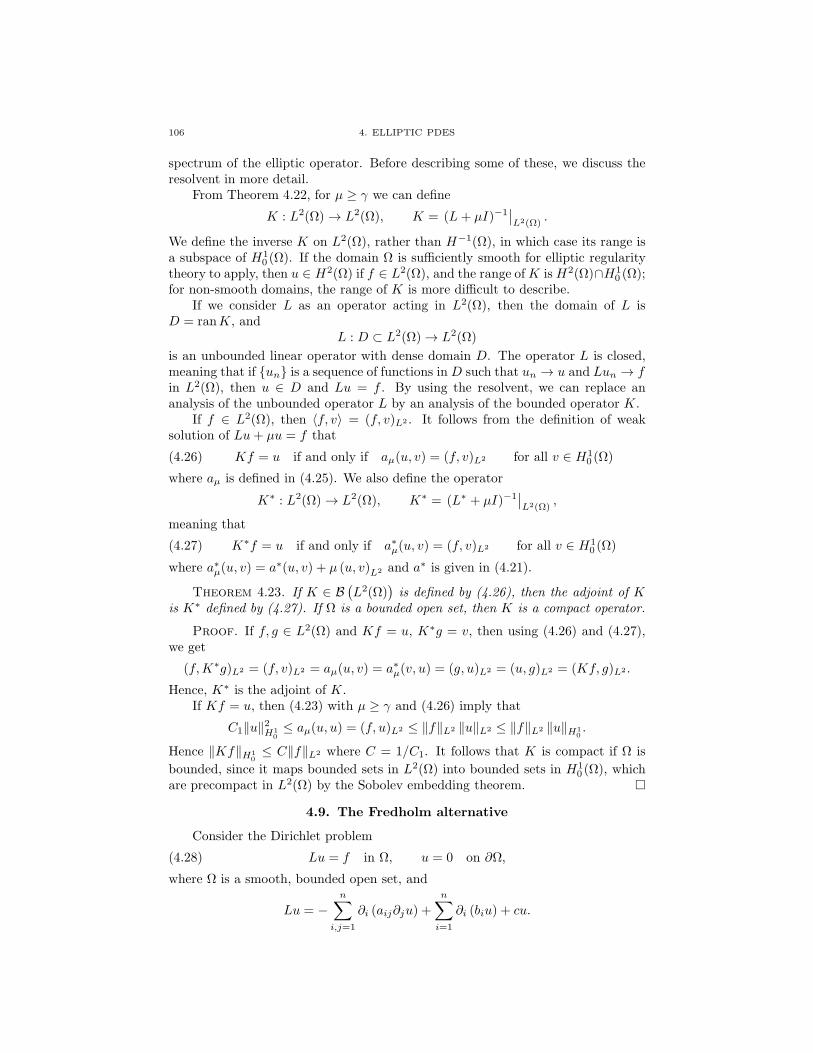
From Theorem 4.22, for µ ≥ γ we can define

K : L2(Ω) → L2(Ω), K = (L + µI)−1∣

∣

L2(Ω).

We define the inverse K on L2(Ω), rather than H−1(Ω), in which case its range isa subspace of H1

0 (Ω). If the domain Ω is sufficiently smooth for elliptic regularitytheory to apply, then u ∈ H2(Ω) if f ∈ L2(Ω), and the range ofK isH2(Ω)∩H1

0 (Ω);for non-smooth domains, the range of K is more difficult to describe.

If we consider L as an operator acting in L2(Ω), then the domain of L isD = ranK, and

L : D ⊂ L2(Ω) → L2(Ω)

is an unbounded linear operator with dense domain D. The operator L is closed,meaning that if un is a sequence of functions in D such that un → u and Lun → fin L2(Ω), then u ∈ D and Lu = f . By using the resolvent, we can replace ananalysis of the unbounded operator L by an analysis of the bounded operator K.

If f ∈ L2(Ω), then 〈f, v〉 = (f, v)L2 . It follows from the definition of weaksolution of Lu+ µu = f that

(4.26) Kf = u if and only if aµ(u, v) = (f, v)L2 for all v ∈ H10 (Ω)

where aµ is defined in (4.25). We also define the operator

K∗ : L2(Ω) → L2(Ω), K∗ = (L∗ + µI)−1∣

∣

L2(Ω),

meaning that

(4.27) K∗f = u if and only if a∗µ(u, v) = (f, v)L2 for all v ∈ H10 (Ω)

where a∗µ(u, v) = a∗(u, v) + µ (u, v)L2 and a∗ is given in (4.21).

Theorem 4.23. If K ∈ B(

L2(Ω))

is defined by (4.26), then the adjoint of Kis K∗ defined by (4.27). If Ω is a bounded open set, then K is a compact operator.

Proof. If f, g ∈ L2(Ω) and Kf = u, K∗g = v, then using (4.26) and (4.27),we get

(f,K∗g)L2 = (f, v)L2 = aµ(u, v) = a∗µ(v, u) = (g, u)L2 = (u, g)L2 = (Kf, g)L2.

Hence, K∗ is the adjoint of K.If Kf = u, then (4.23) with µ ≥ γ and (4.26) imply that

C1‖u‖2H1

0

≤ aµ(u, u) = (f, u)L2 ≤ ‖f‖L2 ‖u‖L2 ≤ ‖f‖L2 ‖u‖H10.

Hence ‖Kf‖H10≤ C‖f‖L2 where C = 1/C1. It follows that K is compact if Ω is

bounded, since it maps bounded sets in L2(Ω) into bounded sets in H10 (Ω), which

are precompact in L2(Ω) by the Sobolev embedding theorem.

4.9. The Fredholm alternative

Consider the Dirichlet problem

(4.28) Lu = f in Ω, u = 0 on ∂Ω,

where Ω is a smooth, bounded open set, and

Lu = −

n∑

i,j=1

∂i (aij∂ju) +

n∑

i=1

∂i (biu) + cu.

4.9. THE FREDHOLM ALTERNATIVE 107

If u = v = 0 on ∂Ω, Green’s formula implies that∫

Ω

(Lu)v dx =

∫

Ω

u (L∗v) dx,

where the formal adjoint L∗ of L is defined by

L∗v = −

n∑

i,j=1

∂i (aij∂jv)−

n∑

i=1

bi∂iv + cv.

It follows that if u is a smooth solution of (4.28) and v is a smooth solution of thehomogeneous adjoint problem,

L∗v = 0 in Ω, v = 0 on ∂Ω,

then∫

Ω

fv dx =

∫

Ω

(Lu)v dx =

∫

Ω

uL∗v dx = 0.

Thus, a necessary condition for (4.28) to be solvable is that f is orthogonal withrespect to the L2(Ω)-inner product to every solution of the homogeneous adjointproblem.

For bounded domains, we will use the compactness of the resolvent to provethat this condition is necessary and sufficient for the existence of a weak solution of(4.28) where f ∈ L2(Ω). Moreover, the solution is unique if and only if a solutionexists for every f ∈ L2(Ω).

This result is a consequence of the fact that if K is compact, then the operatorI+σK is a Fredholm operator with index zero on L2(Ω) for any σ ∈ R, and thereforesatisfies the Fredholm alternative (see Section 4.B.2). Thus, if K = (L + µI)−1 iscompact, the inverse elliptic operator L−λI also satisfies the Fredholm alternative.

Theorem 4.24. Suppose that Ω is a bounded open set in Rn and L is a uni-

formly elliptic operator of the form (4.16) whose coefficients satisfy (4.17). Let L∗

be the adjoint operator (4.22) and λ ∈ R. Then one of the following two alternativesholds.

(1) The only weak solution of the equation L∗v − λv = 0 is v = 0. For everyf ∈ L2(Ω) there is a unique weak solution u ∈ H1

0 (Ω) of the equationLu− λu = f . In particular, the only solution of Lu− λu = 0 is u = 0.

(2) The equation L∗v − λv = 0 has a nonzero weak solution v. The solutionspaces of Lu− λu = 0 and L∗v − λv = 0 are finite-dimensional and havethe same dimension. For f ∈ L2(Ω), the equation Lu − λu = f has aweak solution u ∈ H1

0 (Ω) if and only if (f, v) = 0 for every v ∈ H10 (Ω)

such that L∗v − λv = 0, and if a solution exists it is not unique.

Proof. Since K = (L+ µI)−1 is a compact operator on L2(Ω), the Fredholmalternative holds for the equation

(4.29) u+ σKu = g u, g ∈ L2(Ω)

for any σ ∈ R. Let us consider the two alternatives separately.First, suppose that the only solution of v + σK∗v = 0 is v = 0, which implies

that the only solution of L∗v+(µ+σ)v = 0 is v = 0. Then the Fredholm alterativefor I+σK implies that (4.29) has a unique solution u ∈ L2(Ω) for every g ∈ L2(Ω).In particular, for any g ∈ ranK, there exists a unique solution u ∈ L2(Ω), andthe equation implies that u ∈ ranK. Hence, we may apply L + µI to (4.29),

108 4. ELLIPTIC PDES

and conclude that for every f = (L + µI)g ∈ L2(Ω), there is a unique solutionu ∈ ranK ⊂ H1

0 (Ω) of the equation

(4.30) Lu+ (µ+ σ)u = f.

Taking σ = −(λ+ µ), we get part (1) of the Fredholm alternative for L.Second, suppose that v + σK∗v = 0 has a finite-dimensional subspace of solu-

tions v ∈ L2(Ω). It follows that v ∈ ranK∗ (clearly, σ 6= 0 in this case) and

L∗v + (µ+ σ)v = 0.

By the Fredholm alternative, the equation u + σKu = 0 has a finite-dimensionalsubspace of solutions of the same dimension, and hence so does

Lu+ (µ+ σ)u = 0.

Equation (4.29) is solvable for u ∈ L2(Ω) given g ∈ ranK if and only if

(4.31) (v, g)L2 = 0 for all v ∈ L2(Ω) such that v + σK∗v = 0,

and then u ∈ ranK. It follows that the condition (4.31) with g = Kf is necessaryand sufficient for the solvability of (4.30) given f ∈ L2(Ω). Since

(v, g)L2 = (v,Kf)L2 = (K∗v, f)L2 = −1

σ(v, f)L2

and v + σK∗v = 0 if and only if L∗v + (µ + σ)v = 0, we conclude that (4.30) issolvable for u if and only if f ∈ L2(Ω) satisfies

(v, f)L2 = 0 for all v ∈ ranK such that L∗v + (µ+ σ)v = 0.

Taking σ = −(λ+ µ), we get alternative (2) for L.

Elliptic operators on a Riemannian manifold may have nonzero Fredholm in-dex. The Atiyah-Singer index theorem (1968) relates the Fredholm index of suchoperators with a topological index of the manifold.

4.10. The spectrum of a self-adjoint elliptic operator

Suppose that L is a symmetric, uniformly elliptic operator of the form

(4.32) Lu = −

n∑

i,j=1

∂i (aij∂ju) + cu

where aij = aji and aij , c ∈ L∞(Ω). The associated symmetric bilinear form

a : H10 (Ω)×H1

0 (Ω) → R

is given by

a(u, v) =

∫

Ω

n∑

i,j=1

aij∂iu∂ju+ cuv

dx.

The resolvent K = (L+ µI)−1 is a compact self-adjoint operator on L2(Ω) forsufficiently large µ. Therefore its eigenvalues are real and its eigenfunctions providean orthonormal basis of L2(Ω). Since L has the same eigenfunctions as K, we getthe corresponding result for L.

4.10. THE SPECTRUM OF A SELF-ADJOINT ELLIPTIC OPERATOR 109

Theorem 4.25. The operator L has an increasing sequence of real eigenvaluesof finite multiplicity

λ1 < λ2 ≤ λ3 ≤ · · · ≤ λn ≤ . . .

such that λn → ∞. There is an orthonormal basis φn : n ∈ N of L2(Ω) consistingof eigenfunctions functions φn ∈ H1

0 (Ω) such that

Lφn = λnφn.

Proof. If Kφ = 0 for any φ ∈ L2(Ω), then applying L + µI to the equationwe find that φ = 0, so 0 is not an eigenvalue of K. If Kφ = κφ, for φ ∈ L2(Ω) andκ 6= 0, then φ ∈ ranK and

Lφ =

(

1

κ− µ

)

φ,

so φ is an eigenfunction of L with eigenvalue λ = 1/κ−µ. From Garding’s inequality(4.23) with u = φ, and the fact that a(φ, φ) = λ‖φ‖2L2 , we get

C1‖φ‖2H1

0

≤ (λ+ γ)‖φ‖2L2.

It follows that λ > −γ, so the eigenvalues of L are bounded from below, and atmost a finite number are negative. The spectral theorem for the compact self-adjoint operator K then implies the result.

The boundedness of the domain Ω is essential here, otherwise K need not becompact, and the spectrum of L need not consist only of eigenvalues.

Example 4.26. Suppose that Ω = Rn and L = −∆. Let K = (−∆ + I)−1.

Then, from Example 4.12, K : L2(Rn) → L2(Rn). The range of K is H2(Rn).This operator is bounded but not compact. For example, if φ ∈ C∞

c (Rn) is anynonzero function and aj is a sequence in R

n such that |aj | ↑ ∞ as j → ∞, thenthe sequence φj defined by φj(x) = φ(x − aj) is bounded in L2(Rn) but Kφjhas no convergent subsequence. In this example, K has continuous spectrum [0, 1]on L2(Rn) and no eigenvalues. Correspondingly, −∆ has the purely continuousspectrum [0,∞).

Finally, let us briefly consider the Fredholm alternative for a self-adjoint ellipticequation from the perspective of this spectral theory. The equation

(4.33) Lu− λu = f

may be solved by expansion with respect to the eigenfunctions of L. Suppose thatφn : n ∈ N is an orthonormal basis of L2(Ω) such that Lφn = λnφn, where theeigenvalues λn are increasing and repeated according to their multiplicity. We getthe following alternatives, where all series converge in L2(Ω):

(1) If λ 6= λn for any n ∈ N, then (4.33) has the unique solution

u =

∞∑

n=1

(f, φn)

λn − λφn

for every f ∈ L2(Ω);(2) If λ = λM for for some M ∈ N and λn = λM for M ≤ n ≤ N , then (4.33)

has a solution u ∈ H10 (Ω) if and only if f ∈ L2(Ω) satisfies

(f, φn) = 0 for M ≤ n ≤ N.

110 4. ELLIPTIC PDES

In that case, the solutions are

u =∑

λn 6=λ

(f, φn)

λn − λφn +

N∑

n=M

cnφn

where cM , . . . , cN are arbitrary real constants.

4.11. Interior regularity

Roughly speaking, solutions of elliptic PDEs are as smooth as the data allows.For boundary value problems, it is convenient to consider the regularity of thesolution in the interior of the domain and near the boundary separately. We beginby studying the interior regularity of solutions. We follow closely the presentationin [9].

To motivate the regularity theory, consider the following simple a priori esti-mate for the Laplacian. Suppose that u ∈ C∞

c (Rn). Then, integrating by partstwice, we get

∫

(∆u)2 dx =n∑

i,j=1

∫

(

∂2iiu) (

∂2jju)

dx

= −

n∑

i,j=1

∫

(

∂3iiju)

(∂ju) dx

=

n∑

i,j=1

∫

(

∂2iju) (

∂2iju)

dx

=

∫

∣

∣D2u∣

∣

2dx.

Hence, if −∆u = f , then∥

∥D2u∥

∥

L2 = ‖f‖2L2.

Thus, we can control the L2-norm of all second derivatives of u by the L2-normof the Laplacian of u. This estimate suggests that we should have u ∈ H2

loc iff, u ∈ L2, as is in fact true. The above computation is, however, not justified forweak solutions that belong to H1; as far as we know from the previous existencetheory, such solutions may not even possess second-order weak derivatives.

We will consider a PDE

(4.34) Lu = f in Ω

where Ω is an open set in Rn, f ∈ L2(Ω), and L is a uniformly elliptic of the form

(4.35) Lu = −

n∑

i,j=1

∂i (aij∂ju) .

It is straightforward to extend the proof of the regularity theorem to uniformlyelliptic operators that contain lower-order terms [9].

A function u ∈ H1(Ω) is a weak solution of (4.34)–(4.35) if

(4.36) a(u, v) = (f, v) for all v ∈ H10 (Ω),

4.11. INTERIOR REGULARITY 111

where the bilinear form a is given by

(4.37) a(u, v) =

n∑

i,j=1

∫

Ω

aij∂iu∂jv dx.

We do not impose any boundary condition on u, for example by requiring thatu ∈ H1

0 (Ω), so the interior regularity theorem applies to any weak solution of(4.34).

Before stating the theorem, we illustrate the idea of the proof with a furthera priori estimate. To obtain a local estimate for D2u on a subdomain Ω′ ⋐ Ω, weintroduce a cut-off function η ∈ C∞

c (Ω) such that 0 ≤ η ≤ 1 and η = 1 on Ω′. Wetake as a test function

(4.38) v = −∂k(

η2∂ku)

.

Note that v is given by a positive-definite, symmetric operator acting on u of asimilar form to L, which leads to the positivity of the resulting estimate for D∂ku.

Multiplying (4.34) by v and integrating over Ω, we get (Lu, v) = (f, v). Twointegrations by parts imply that

(Lu, v) =

n∑

i,j=1

∫

Ω

∂j (aij∂iu)(

∂kη2∂ku

)

dx

=

n∑

i,j=1

∫

Ω

∂k (aij∂iu)(

∂jη2∂ku

)

dx

=

n∑

i,j=1

∫

Ω

η2aij (∂i∂ku) (∂j∂ku) dx+ F

where

F =n∑

i,j=1

∫

Ω

η2 (∂kaij) (∂iu) (∂j∂ku)

+ 2η∂jη[

aij (∂i∂ku) (∂ku) + (∂kaij) (∂iu) (∂ku)]

dx.

The term F is linear in the second derivatives of u. We use the uniform ellipticityof L to get

θ

∫

Ω′

|D∂ku|2 dx ≤

n∑

i,j=1

∫

Ω

η2aij (∂i∂ku) (∂j∂ku) dx = (f, v)− F,

and a Cauchy inequality with ǫ to absorb the linear terms in second derivatives onthe right-hand side into the quadratic terms on the left-hand side. This results inan estimate of the form

‖D∂ku‖2L2(Ω′) ≤ C

(

‖f‖2L2(Ω) + ‖u‖2H1(Ω)

)

.

The proof of regularity is entirely analogous, with the derivatives in the test function(4.38) replaced by difference quotients (see Section 4.C). We obtain an L2(Ω′)-bound for the difference quotients D∂hku that is uniform in h, which implies thatu ∈ H2(Ω′).

112 4. ELLIPTIC PDES

Theorem 4.27. Suppose that Ω is an open set in Rn. Assume that aij ∈ C1(Ω)

and f ∈ L2(Ω). If u ∈ H1(Ω) is a weak solution of (4.34)–(4.35), then u ∈ H2(Ω′)for every Ω′ ⋐ Ω. Furthermore,

(4.39) ‖u‖H2(Ω′) ≤ C(

‖f‖L2(Ω) + ‖u‖L2(Ω)

)

where the constant C depends only on n, Ω′, Ω and aij .

Proof. Choose a cut-off function η ∈ C∞c (Ω) such that 0 ≤ η ≤ 1 and η = 1

on Ω′. We use the compactly supported test function

v = −D−hk

(

η2Dhku)

∈ H10 (Ω)

in the definition (4.36)–(4.37) for weak solutions. (As in (4.38), v is given by apositive self-adjoint operator acting on u.) This implies that

(4.40) −n∑

i,j=1

∫

Ω

aij (∂iu)D−hk ∂j

(

η2Dhku)

dx = −

∫

Ω

fD−hk

(

η2Dhku)

dx.

Performing a discrete integration by parts and using the product rule, we may writethe left-hand side of (4.40) as

−

n∑

i,j=1

∫

Ω

aij (∂iu)D−hk ∂j

(

η2Dhku)

dx =

n∑

i,j=1

∫

Ω

Dhk (aij∂iu) ∂j

(

η2Dhku)

dx

=

n∑

i,j=1

∫

Ω

η2ahij(

Dhk∂iu

) (

Dhk∂ju

)

dx+ F,

(4.41)

with ahij(x) = aij(x+ hek), where the error-term F is given by

F =n∑

i,j=1

∫

Ω

η2(

Dhkaij

)

(∂iu)(

Dhk∂ju

)

+ 2η∂jη[

ahij(

Dhk∂iu

) (

Dhku)

+(

Dhkaij

)

(∂iu)(

Dhku)

]

dx.

(4.42)

Using the uniform ellipticity of L in (4.18), we estimate

θ

∫

Ω

η2∣

∣DhkDu

∣

∣

2dx ≤

n∑

i,j=1

∫

Ω

η2ahij(

Dhk∂iu

) (

Dhk∂ju

)

dx.

Using (4.40)–(4.41) and this inequality, we find that

(4.43) θ

∫

Ω

η2∣

∣DhkDu

∣

∣

2dx ≤ −

∫

Ω

fD−hk

(

η2Dhku)

dx− F.

By the Cauchy-Schwartz inequality,∣

∣

∣

∣

∫

Ω

fD−hk

(

η2Dhku)

dx

∣

∣

∣

∣

≤ ‖f‖L2(Ω)

∥

∥D−hk

(

η2Dhku)∥

∥

L2(Ω).

Since supp η ⋐ Ω, Theorem 4.53 implies that for sufficiently small h,∥

∥D−hk

(

η2Dhku)∥

∥

L2(Ω)≤∥

∥∂k(

η2Dhku)∥

∥

L2(Ω)

≤∥

∥η2∂kDhku∥

∥

L2(Ω)+∥

∥2η (∂kη)Dhku∥

∥

L2(Ω)

≤∥

∥η∂kDhku∥

∥

L2(Ω)+ C ‖Du‖L2(Ω) .

4.11. INTERIOR REGULARITY 113

A similar estimate of F in (4.42) gives

|F | ≤ C(

‖Du‖L2(Ω)

∥

∥ηDhkDu

∥

∥

L2(Ω)+ ‖Du‖

2L2(Ω)

)

.

Using these results in (4.43), we find that

θ∥

∥ηDhkDu

∥

∥

2

L2(Ω)≤C(

‖f‖L2(Ω)

∥

∥ηDhkDu

∥

∥

L2(Ω)+ ‖f‖L2(Ω) ‖Du‖L2(Ω)

+ ‖Du‖L2(Ω)

∥

∥ηDhkDu

∥

∥

L2(Ω)+ ‖Du‖

2L2(Ω)

)

.(4.44)

By Cauchy’s inequality with ǫ, we have

‖f‖L2(Ω)

∥

∥ηDhkDu

∥

∥

L2(Ω)≤ ǫ

∥

∥ηDhkDu

∥

∥

2

L2(Ω)+

1

4ǫ‖f‖

2L2(Ω) ,

‖Du‖L2(Ω)

∥

∥ηDhkDu

∥

∥

L2(Ω)≤ ǫ

∥

∥ηDhkDu

∥

∥

2

L2(Ω)+

1

4ǫ‖Du‖

2L2(Ω) .

Hence, choosing ǫ so that 4Cǫ = θ, and using the result in (4.44) we get that

θ

4

∥

∥ηDhkDu

∥

∥

2

L2(Ω)≤ C

(

‖f‖2L2(Ω) + ‖Du‖2L2(Ω)

)

.

Thus, since η = 1 on Ω′,

(4.45)∥

∥DhkDu

∥

∥

2

L2(Ω′)≤ C

(

‖f‖2L2(Ω) + ‖Du‖

2L2(Ω)

)

where the constant C depends on Ω, Ω′, aij , but is independent of h, u, f . The-orem 4.53 now implies that the weak second derivatives of u exist and belong toL2(Ω). Furthermore, the H2-norm of u satisfies

‖u‖H2(Ω′) ≤ C(

‖f‖L2(Ω) + ‖u‖H1(Ω)

)

.

Finally, we replace ‖u‖H1(Ω) in this estimate by ‖u‖L2(Ω). First, by the previousargument, if Ω′ ⋐ Ω′′ ⋐ Ω, then

(4.46) ‖u‖H2(Ω′) ≤ C(

‖f‖L2(Ω′′) + ‖u‖H1(Ω′′)

)

.

Let η ∈ C∞c (Ω) be a cut-off function with 0 ≤ η ≤ 1 and η = 1 on Ω′′. Using the

uniform ellipticity of L and taking v = η2u in (4.36)–(4.37), we get that

θ

∫

Ω

η2|Du|2 dx ≤

n∑

i,j=1

∫

Ω

η2aij∂iu∂ju dx

≤

∫

Ω

η2fu dx−

n∑

i,j=1

∫

Ω

2aijηu∂iu∂jη dx

≤ ‖f‖L2(Ω)‖u‖L2(Ω) + C‖u‖L2(Ω)‖ηDu‖L2(Ω).

Cauchy’s inequality with ǫ then implies that

‖ηDu‖2L2(Ω) ≤ C(

‖f‖2L2(Ω) + ‖u‖2L2(Ω)

)

,

and since ‖Du‖2L2(Ω′′) ≤ ‖ηDu‖2L2(Ω), the use of this result in (4.46) gives (4.39).

If u ∈ H2loc(Ω) and f ∈ L2(Ω), then the equation Lu = f relating the weak

derivatives of u and f holds pointwise a.e.; such solutions are often called strongsolutions, to distinguish them from weak solutions, which may not possess weaksecond order derivatives, and classical solutions, which possess continuous secondorder derivatives.

The repeated application of these estimates leads to higher interior regularity.

114 4. ELLIPTIC PDES

Theorem 4.28. Suppose that aij ∈ Ck+1(Ω) and f ∈ Hk(Ω). If u ∈ H1(Ω) is aweak solution of (4.34)–(4.35), then u ∈ Hk+2(Ω′) for every Ω′ ⋐ Ω. Furthermore,

‖u‖Hk+2(Ω′) ≤ C(

‖f‖Hk(Ω) + ‖u‖L2(Ω)

)

where the constant C depends only on n, k, Ω′, Ω and aij .

See [9] for a detailed proof. Note that if the above conditions hold with k > n/2,then f ∈ C(Ω) and u ∈ C2(Ω), so u is a classical solution of the PDE Lu = f .Furthermore, if f and aij are smooth then so is the solution.

Corollary 4.29. If aij , f ∈ C∞(Ω) and u ∈ H1(Ω) is a weak solution of(4.34)–(4.35), then u ∈ C∞(Ω)

Proof. If Ω′⋐ Ω, then f ∈ Hk(Ω′) for every k ∈ N, so by Theorem (4.28)

u ∈ Hk+2loc (Ω′) for every k ∈ N, and by the Sobolev embedding theorem u ∈ C∞(Ω′).

Since this holds for every open set Ω′ ⋐ Ω, we have u ∈ C∞(Ω).

4.12. Boundary regularity

To study the regularity of solutions near the boundary, we localize the problemto a neighborhood of a boundary point by use of a partition of unity: We decomposethe solution into a sum of functions that are compactly supported in the sets of asuitable open cover of the domain and estimate each function in the sum separately.

Assuming, as in Section 1.10, that the boundary is at least C1, we may ‘flatten’the boundary in a neighborhood U by a diffeomorphism ϕ : U → V that maps U∩Ωto an upper half space V = B1 (0)∩ yn > 0. If ϕ−1 = ψ and x = ψ(y), then by achange of variables (c.f. Theorem 1.44 and Proposition 3.21) the weak formulation(4.34)–(4.35) on U becomes

n∑

i,j=1

∫

V

aij∂u

∂yi

∂v

∂yjdy =

∫

V

f v dy for all functions v ∈ H10 (V ),

where u ∈ H1(V ). Here, u = u ψ, v = v ψ, and

aij = |detDψ|

n∑

p,q=1

apq ψ

(

∂ϕi

∂xp ψ

)(

∂ϕj

∂xq ψ

)

, f = |detDψ| f ψ.

The matrix aij satisfies the uniform ellipticity condition if apq does. To see this,we define ζ = (Dϕt) ξ, or

ζp =

n∑

i=1

∂ϕi

∂xpξi.

Then, since Dϕ and Dψ = Dϕ−1 are invertible and bounded away from zero, wehave for some constant C > 0 that

n∑

i,j=1

aijξiξj = |detDψ|

n∑

p,q=1

apqζpζq ≥ |detDψ| θ|ζ|2 ≥ Cθ|ξ|2.

Thus, we obtain a problem of the same form as before after the change of variables.Note that we must require that the boundary is C2 to ensure that aij is C1.

It is important to recognize that in changing variables for weak solutions, weneed to verify the change of variables for the weak formulation directly and notjust for the original PDE. A transformation that is valid for smooth solutions of a

4.12. BOUNDARY REGULARITY 115

PDE is not always valid for weak solutions, which may lack sufficient smoothnessto justify the transformation.

We now state a boundary regularity theorem. Unlike the interior regularitytheorem, we impose a boundary condition u ∈ H1

0 (Ω) on the solution, and we re-quire that the boundary of the domain is smooth. A solution of an elliptic PDEwith smooth coefficients and smooth right-hand side is smooth in the interior ofits domain of definition, whatever its behavior near the boundary; but we can-not expect to obtain smoothness up to the boundary without imposing a smoothboundary condition on the solution and requiring that the boundary is smooth.

Theorem 4.30. Suppose that Ω is a bounded open set in Rn with C2-boundary.

Assume that aij ∈ C1(Ω) and f ∈ L2(Ω). If u ∈ H10 (Ω) is a weak solution of

(4.34)–(4.35), then u ∈ H2(Ω), and

‖u‖H2(Ω) ≤ C(

‖f‖L2(Ω) + ‖u‖L2(Ω)

)

where the constant C depends only on n, Ω and aij.

Proof. By use of a partition of unity and a flattening of the boundary, it issufficient to prove the result for an upper half space Ω = (x1, . . . , xn) : xn > 0space and functions u, f : Ω → R that are compactly supported in B1 (0) ∩ Ω. Letη ∈ C∞

c (Rn) be a cut-off function such that 0 ≤ η ≤ 1 and η = 1 on B1 (0). Wewill estimate the tangential and normal difference quotients of Du separately.

First consider a test function that depends on tangential differences,

v = −D−hk η2Dh

ku for k = 1, 2, . . . , n− 1.

Since the trace of u is zero on ∂Ω, the trace of v on ∂Ω is zero and, by Theorem 3.44,v ∈ H1

0 (Ω). Thus we may use v in the definition of weak solution to get (4.40).Exactly the same argument as the one in the proof of Theorem 4.27 gives (4.45).It follows from Theorem 4.53 that the weak derivatives ∂k∂iu exist and satisfy

(4.47) ‖∂kDu‖L2(Ω) ≤ C(

‖f‖L2(Ω) + ‖u‖L2(Ω)

)

for k = 1, 2, . . . , n− 1.

The only derivative that remains is the second-order normal derivative ∂2nu,which we can estimate from the equation. Using (4.34)–(4.35), we have for φ ∈C∞

c (Ω) that∫

Ω

ann (∂nu) (∂nφ) dx = −∑′

∫

Ω

aij (∂iu) (∂jφ) dx+

∫

Ω

fφ dx

where∑′

denotes the sum over 1 ≤ i, j ≤ n with the term i = j = n omitted. Sinceaij ∈ C1(Ω) and ∂iu is weakly differentiable with respect to xj unless i = j = n weget, using Proposition 3.21, that∫

Ω

ann (∂nu) (∂nφ) dx =∑′

∫

Ω

∂j [aij (∂iu)] + fφdx for every φ ∈ C∞c (Ω).

It follows that ann (∂nu) is weakly differentiable with respect to xn, and

∂n [ann (∂nu)] = −

∑′∂j [aij (∂iu)] + f

∈ L2(Ω).

From the uniform ellipticity condition (4.18) with ξ = en, we have ann ≥ θ. Hence,by Proposition 3.21,

∂nu =1

annann∂nu

116 4. ELLIPTIC PDES

is weakly differentiable with respect to xn with derivative

∂2nnu =1

ann∂n [ann∂nu] + ∂n

(

1

ann

)

ann∂nu ∈ L2(Ω).

Furthermore, using (4.47) we get an estimate of the same form for ‖∂2nnu‖2L2(Ω), so

that∥

∥D2u∥

∥

L2(Ω)≤ C

(

‖f‖2L2(Ω) + ‖u‖2L2(Ω)

)

The repeated application of these estimates leads to higher-order regularity.

Theorem 4.31. Suppose that Ω is a bounded open set in Rn with Ck+2-

boundary. Assume that aij ∈ Ck+1(Ω) and f ∈ Hk(Ω). If u ∈ H10 (Ω) is a weak

solution of (4.34)–(4.35), then u ∈ Hk+2(Ω) and

‖u‖Hk+2(Ω) ≤ C(

‖f‖Hk(Ω) + ‖u‖L2(Ω)

)

where the constant C depends only on n, k, Ω, and aij .

Sobolev embedding then yields the following result.

Corollary 4.32. Suppose that Ω is a bounded open set in Rn with C∞ bound-

ary. If aij , f ∈ C∞(Ω) and u ∈ H10 (Ω) is a weak solution of (4.34)–(4.35), then

u ∈ C∞(Ω)

4.13. Some further perspectives

This book is to a large extent self-contained, with the restrictionthat the linear theory — Schauder estimates and Campanatotheory — is not presented. The reader is expected to be famil-iar with functional-analytic tools, like the theory of monotoneoperators.4

The above results give an existence and L2-regularity theory for second-order,uniformly elliptic PDEs in divergence form. This theory is based on the simplea priori energy estimate for ‖Du‖L2 that we obtain by multiplying the equationLu = f by u, or some derivative of u, and integrating the result by parts.

This theory is a fundamental one, but there is a bewildering variety of ap-proaches to the existence and regularity of solutions of elliptic PDEs. In an at-tempt to put the above analysis in a broader context, we briefly list some of theseapproaches and other important results, without any claim to completeness. Manyof these topics are discussed further in the references [9, 17, 23].

Lp-theory: If 1 < p < ∞, there is a similar regularity result that solutionsof Lu = f satisfy u ∈ W 2,p if f ∈ Lp. The derivation is not as simple whenp 6= 2, however, and requires the use of more sophisticated tools from realanalysis (such as the Lp-theory of Calderon-Zygmund operators).

Schauder theory: The Schauder theory provides Holder-estimates similarto those derived in Section 2.7.2 for Laplace’s equation, and a correspond-ing existence theory of solutions u ∈ C2,α of Lu = f if f ∈ C0,α and L hasHolder continuous coefficients. General linear elliptic PDEs are treatedby regarding them as perturbations of constant coefficient PDEs, an ap-proach that works because there is no ‘loss of derivatives’ in the estimates

4From the introduction to [2].

4.13. SOME FURTHER PERSPECTIVES 117

of the solution. The Holder estimates were originally obtained by the useof potential theory, but other ways to obtain them are now known; forexample, by the use of Campanato spaces, which provide Holder normsin terms of suitable integral norms that are easier to estimate directly.

Perron’s method: Perron (1923) showed that solutions of the Dirichletproblem for Laplace’s equation can be obtained as the infimum of super-harmonic functions or the supremum of subharmonic functions, togetherwith the use of barrier functions to prove that, under suitable assumptionson the boundary, the solution attains the prescribed boundary values.This method is based on maximum principle estimates.

Boundary integral methods: By the use of Green’s functions, one canoften reduce a linear elliptic BVP to an integral equation on the boundary,and then use the theory of integral equations to study the existence andregularity of solutions. These methods also provide efficient numericalschemes because of the lower dimensionality of the boundary.

Pseudo-differential operators: The Fourier transform provides an effec-tive method for solving linear PDEs with constant coefficients. The theoryof pseudo-differential and Fourier-integral operators is a powerful exten-sion of this method that applies to general linear PDEs with variablecoefficients, and elliptic PDEs in particular. It is, however, less well-suited to the analysis of nonlinear PDEs (although there are nonlineargenerlizations, such as the theory of para-differential operators).

Variational methods: Many elliptic PDEs — especially those in diver-gence form — arise as Euler-Lagrange equations for variational princi-ples. Direct methods in the calculus of variations provide a powerful andgeneral way to analyze such PDEs, both linear and nonlinear.

Di Giorgi-Nash-Moser: Di Giorgi (1957), Nash (1958), and Moser (1960)showed that weak solutions of a second order elliptic PDE in divergenceform with bounded (L∞) coefficients are Holder continuous (C0,α). Thiswas the key step in developing a regularity theory for minimizers of non-linear variational principles with elliptic Euler-Lagrange equations. Moseralso obtained a Harnack inequality for weak solutions which is a crucialingredient of the regularity theory.

Fully nonlinear equations: Krylov and Safonov (1979) obtained a Har-nack inequality for second order elliptic equations in nondivergence form.This allowed the development of a regularity theory for fully nonlinearelliptic equations (e.g. second-order equations for u that depend nonlin-early on D2u). Crandall and Lions (1983) introduced the notion of viscos-ity solutions which — despite the name — uses the maximum principleand is based on a comparison with appropriate sub and super solutionsThis theory applies to fully nonlinear elliptic PDEs, although it is mainlyrestricted to scalar equations.

Degree theory: Topological methods based on the Leray-Schauder degreeof a mapping on a Banach space can be used to prove existence of solutionsof various nonlinear elliptic problems [32]. These methods can provideglobal existence results for large solutions, but often do not give muchdetailed analytical information about the solutions.

118 4. ELLIPTIC PDES

Heat flow methods: Parabolic PDEs, such as ut + Lu = f , are closelyconnected with the associated elliptic PDEs for stationary solutions, suchas Lu = f . One may use this connection to obtain solutions of an ellip-tic PDE as the limit as t → ∞ of solutions of the associated parabolicPDE. For example, Hamilton (1981) introduced the Ricci flow on a man-ifold, in which the metric approaches a Ricci-flat metric as t → ∞, as ameans to understand the topological classification of smooth manifolds,and Perelman (2003) used this approach to prove the Poincare conjecture(that every simply connected, three-dimensional, compact manifold with-out boundary is homeomorphic to a three-dimensional sphere) and, moregenerally, the geometrization conjecture of Thurston.