Vigilance behavior and land use by sandhill cranes (grus ...
59
Eastern Michigan University DigitalCommons@EMU Master's eses and Doctoral Dissertations Master's eses, and Doctoral Dissertations, and Graduate Capstone Projects 2009 Vigilance behavior and land use by sandhill cranes (grus canadensis) Trevor Eldred Follow this and additional works at: hp://commons.emich.edu/theses Part of the Biology Commons is Open Access esis is brought to you for free and open access by the Master's eses, and Doctoral Dissertations, and Graduate Capstone Projects at DigitalCommons@EMU. It has been accepted for inclusion in Master's eses and Doctoral Dissertations by an authorized administrator of DigitalCommons@EMU. For more information, please contact [email protected]. Recommended Citation Eldred, Trevor, "Vigilance behavior and land use by sandhill cranes (grus canadensis)" (2009). Master's eses and Doctoral Dissertations. 238. hp://commons.emich.edu/theses/238
Transcript of Vigilance behavior and land use by sandhill cranes (grus ...

Eastern Michigan UniversityDigitalCommons@EMU
Master's Theses and Doctoral Dissertations Master's Theses, and Doctoral Dissertations, andGraduate Capstone Projects
2009
Vigilance behavior and land use by sandhill cranes(grus canadensis)Trevor Eldred
Follow this and additional works at: http://commons.emich.edu/theses
Part of the Biology Commons
This Open Access Thesis is brought to you for free and open access by the Master's Theses, and Doctoral Dissertations, and Graduate Capstone Projectsat DigitalCommons@EMU. It has been accepted for inclusion in Master's Theses and Doctoral Dissertations by an authorized administrator ofDigitalCommons@EMU. For more information, please contact [email protected].
Recommended CitationEldred, Trevor, "Vigilance behavior and land use by sandhill cranes (grus canadensis)" (2009). Master's Theses and DoctoralDissertations. 238.http://commons.emich.edu/theses/238

Vigilance Behavior and Land Use by Sandhill Cranes (Grus canadensis)
By
Trevor Eldred
Thesis
Submitted to the Department of Biology
Eastern Michigan University
In partial fulfillment of the requirements
For the degree of
MASTER OF SCIENCE
In
Biology with a concentration in Organismal Biology
Thesis Committee:
Peter Bednekoff, PhD, Chair
Allen Kurta, PhD
Cara Shillington, PhD
May 3, 2009
Ypsilanti, Michigan

Abstract
I investigated how vigilance in sandhill crane time budgets changed with
behavioral, climatic, and anthropogenic factors. I measured two different postures that
could be interpreted as vigilance. Cranes significantly altered the time spent in the alert
investigative posture with differences in gender and modal non-vigilant behavior. They
significantly altered the time spent in the tall alert posture with differences in gender,
breeding status, time of day, traffic on the nearest road, and human disturbances. The
southern Michigan populations of sandhill cranes nest closer to roads and houses than
they have in the past and do not preferentially avoid them. They favor emergent and
semi-permanently flooded wetlands and avoid forested, open water, and scrub-shrub
wetlands for nesting. They do not preferentially avoid roads and houses when selecting
fall staging sites. Sandhill crane vigilance is best determined by the alert investigative
posture, although this posture may include other behaviors as well. Sandhill cranes
adapt well to human impacts, and their population can increase with their ability to move
beyond the traditional nesting and migratory staging sites.
2

Introduction
Sandhill Crane Natural History
Sandhill cranes (Grus canadensis) are tall, wetland-nesting birds found across
much of North America. There are six subspecies (Tacha et al. 1992), the largest of
which (G. c. tabida) nests in Michigan (Walkinshaw, 1949). Cranes are omnivorous.
They eat row crops, primarily corn and wheat, as well as snails, slugs, grasshoppers,
worms, crayfish, small mammals, frogs, snakes, and chicks and eggs of other birds
(Tacha et al., 1992). They mate for life, return to the same nesting territory every year,
and often reuse the same nest sites (Walkinshaw, 1989). They nest on the ground,
commonly in emergent wetlands, and make their nests out of available plant material in
the immediate vicinity (Walkinshaw, 1949; Drewien, 1973; Tacha, et al., 1992). They
prefer to nest in wetlands dominated by cattail (Typha spp.) or sedges (Carex spp.)
(Walkinshaw, 1973).
Crows and raccoons are the most destructive predators of nest and young,
though ravens, foxes, and coyotes also prey on crane eggs and young (Drewien, 1973).
When ground predators are experimentally removed, crane productivity increases
(Littlefield, 2003).
Cranes nest in the spring and produce two (rarely one or three) eggs per year,
for which both parents share incubating duties (Walkinshaw, 1949, Drewien, 1973).
Incubation is about 30 days, and in Michigan chicks typically hatch in May and June
(Walkinshaw, 1949). Cranes are territorial during the nesting season, when the males
3

do slightly more territory maintenance and the females do slightly more parental care for
the offspring (Tacha, 1988; Meine and Archibald, 1996).
As the chicks fledge, family units become less territorial and cranes form large
flocks where they prepare for fall migration (Walkinshaw, 1973). This flocking behavior
is called staging. These flocks roost in large wetlands at night. Cranes will fly up to 5
miles (8000 meters) from the staging wetland to forage (Provost, 1991). The Michigan
population of sandhill cranes migrates to Florida and Georgia for the winter (Tacha et
al., 1992). This occurs between October and December, with some individuals
returning to Michigan as early as February (pers. obs.). A juvenile crane will stay with
its parents for 10 months (Tacha, 1988), but Michigan cranes do not mate until they
reach three years old (Walkinshaw, 1973). During these three years young cranes form
non-territorial flocks of non-breeding birds; hence flocks of cranes can be found at all
times of the year where cranes are present. These flocks cause some crop damage,
especially to corn, although the extent of this probably varies with geographic region
(Halbeisen 1980, McIvor and Conover 1994).
The Southern Michigan Sandhill Crane Population
The sandhill crane population has increased sharply in Michigan over the past 75
years following a ban on hunting. In 1931, Walkinshaw (1949) estimated that there
were 17 breeding pairs in southern Michigan; by 1946 the number had increased to 27
pairs (Walkinshaw, 1949). In 1952, a more comprehensive survey found 49 breeding
pairs (Walkinshaw and Wing, 1955), and by 1973, 151 pairs were found (Walkinshaw
and Hoffman, 1974). In 1987, 642 pairs were known in southern Michigan (Hoffman,
4

1989). Although some of the increase in known pairs is likely due to greater awareness
of cranes and increased effectiveness of sampling methods, without doubt the sandhill
crane population of Michigan has increased sharply.
With this increase in crane population, cranes have come into increasing contact
with humans. In the past it was thought that sandhill cranes avoided human presence,
preferring to nest in large, isolated wetlands (Walkinshaw, 1949). Since then, cranes
have increasingly bred in wetland closer to roads and houses (Hoffman, 1983).
Habitat Studies
Many studies have been conducted on sandhill crane nest site characteristics,
nesting success, and general population demographics in a given region (Burke, 2001;
Provost, 1991; Drewien, 1973). Likewise, there have been several studies on general
habitat characteristics that may influence habitat (nesting wetland) choice (Su, 2003;
Provost, 1991; Drewien, 1973). On the Michigan population, Hoffman (1983) found that
between 1970 and 1982, the average nesting wetland size decreased from 58 to 38 ha,
65% of nesting wetlands were associated with open water, the distance to the nearest
road decreased by 20%, and the distance to the nearest residence decreased by 26%
(n = 26). While there has been some research conducted on habitat use by cranes,
little research has been conducted on the habitat components of fall staging areas.
Furthermore, no large-scale study of sandhill crane habitat use in the southern Michigan
population has been conducted in over 25 years.
5

Vigilance
Vigilance is an important factor in the time budget of any animal. It is widely
known that vigilance increases with increased predation risk (Bednekoff and Lima,
1998). Sandhill cranes have two postures that can be associated with acts of vigilance.
In cranes these postures are defined as “alert investigative” and “tall alert,” while in
geese they are called “head up” and “extreme head up” respectively (Tacha, 1988;
Lazarus and Inglis, 1978). Voss (1976) also defined them as “standing/resting,” and
“alert” postures. A crane standing, or rarely sitting with its head up and bill held
horizontally but its neck not fully extended, characterizes the alert investigative posture.
The crane is apparently looking around and may also be walking slowly during this
behavior. A crane standing erect with its neck fully outstretched, presumably for a taller
vantage point, characterizes the tall alert posture. This behavior is often directionally
oriented, and a crane typically does not walk during this behavior. Previous
investigations of the tall alert posture indicate that in cranes, it is usually directed toward
a specific, known disturbance in the environment (Tacha, 1988; Voss, 1976). Tacha
(1988) also notes that this behavior can be contagious in a flock.
Previous workers have disagreed on to what degree these postures are vigilance
versus other purposes such as checking on young, attentiveness to other conspecifics,
or scanning for food. Voss (1976) interpreted the alert investigative posture as a mere
resting position with no vigilance associated with it. The tall alert posture was defined
as the vigilant posture in this case. Tacha (1988) interpreted the alert investigative
posture as a posture indicating that the cranes were “not obviously alarmed, but
appeared inquisitive about something in the environment.” This is close to a traditional
6
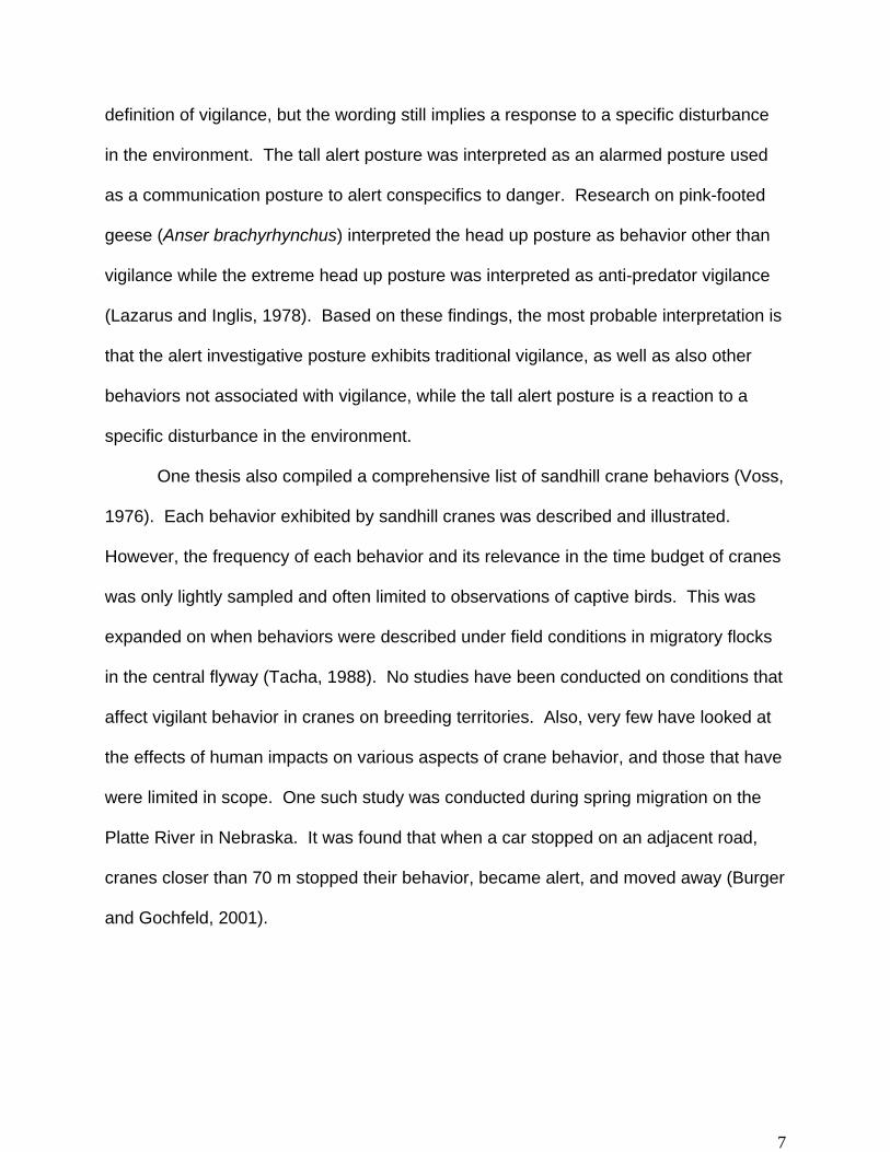
definition of vigilance, but the wording still implies a response to a specific disturbance
in the environment. The tall alert posture was interpreted as an alarmed posture used
as a communication posture to alert conspecifics to danger. Research on pink-footed
geese (Anser brachyrhynchus) interpreted the head up posture as behavior other than
vigilance while the extreme head up posture was interpreted as anti-predator vigilance
(Lazarus and Inglis, 1978). Based on these findings, the most probable interpretation is
that the alert investigative posture exhibits traditional vigilance, as well as also other
behaviors not associated with vigilance, while the tall alert posture is a reaction to a
specific disturbance in the environment.
One thesis also compiled a comprehensive list of sandhill crane behaviors (Voss,
1976). Each behavior exhibited by sandhill cranes was described and illustrated.
However, the frequency of each behavior and its relevance in the time budget of cranes
was only lightly sampled and often limited to observations of captive birds. This was
expanded on when behaviors were described under field conditions in migratory flocks
in the central flyway (Tacha, 1988). No studies have been conducted on conditions that
affect vigilant behavior in cranes on breeding territories. Also, very few have looked at
the effects of human impacts on various aspects of crane behavior, and those that have
were limited in scope. One such study was conducted during spring migration on the
Platte River in Nebraska. It was found that when a car stopped on an adjacent road,
cranes closer than 70 m stopped their behavior, became alert, and moved away (Burger
and Gochfeld, 2001).
7

Hypotheses
I investigated the time budget of cranes, specifically how vigilance behaviors are
affected by various spatial and temporal factors. A better understanding of what factors
contribute to vigilant behavior can aid in management for a growing crane population. I
also attempt to update the status of the sandhill crane population in southern Michigan.
Within this I examined habitat patch use by breeding and non-breeding cranes,
specifically nesting wetland use. I attempted to quantify habitat use as it relates to
human impacts and wetland characteristics.
My specific aims were 1) to determine what life history, environmental, and
anthropogenic factors contribute to vigilant behavior in cranes; 2) to quantify the
association of and differences between the alert investigative and tall alert postures in
cranes; 3) to determine what habitat features of wetlands are important in nesting
wetland choice by cranes; 4) to determine what anthropogenic land use characteristics
are important for wetland nesting choice by cranes; and 5) to determine what habitat
characteristics are important in wetland choice for fall staging wetlands.
8

Materials and Methods
Study Area
During the nesting season, the study area was 145.5 square miles in
northeastern Jackson County, Michigan, including Waterloo and Henrietta Townships,
as well as parts of Grass Lake and Leoni Townships. This area consisted of 37%
farmland, 21% upland forest, and 26% wetland (Michigan Department of Natural
Resources, 2001). The farmland consisted primarily of row crops, mainly corn, soy, and
wheat (pers. obs.). Some hay and dairy farming also occurred. Mean population
density in the primary study area was 158 people per square mile overall, but only 82
people per square mile outside of developed residential areas. These developed
residential areas in the primary study area were small and consisted mainly of the
villages of Clear Lake, Grass Lake, Waterloo, Munith, and Pleasant Lake. The city of
Jackson was located 3 to 15 miles from the study area; and a major Interstate highway
(I-94) runs through it. Waterloo State Recreation Area comprised a major part of the
study area, and much of the undeveloped land (wetland and forest) was located within
the Recreation Area boundary.
Within this study area is located Haehnle Audubon Sanctuary, a sanctuary
founded in 1955 specifically to protect sandhill cranes. In 2005 the large emergent
marsh at the center of the sanctuary supported at least five breeding pairs of sandhill
cranes, as well as a flock of non-breeding cranes. In the fall, this wetland also served
as one of the primary migratory staging areas for cranes in Michigan. It had been
censused for cranes periodically since 1935, with annual detailed counts posted on the
Sanctuary website dating back to 1969 (Jackson Audubon Society, 2006). The primary
9

study area has been described extensively elsewhere (Halbeisan, 1980; Hoffman, 1983;
Hoffman, 1989) and has been reported in the past to have the highest nesting density of
sandhill cranes in the nation (Hoffman, 1983).
For fall staging, due to the relatively small number of fall staging locations, the
primary study area was expanded to include all of Jackson County. Jackson County is
located in south-central Michigan and has one major metropolitan center (Jackson).
Land use in Jackson County was primarily agricultural (50%), with wetlands (21%),
upland forest (20%), developed land (6%), and open water (2%) comprising the majority
of the remainder of the land (Michigan Center for Geographic Information, 2002).
Wetland and Land Use Definitions
Wetland classes were defined in four categories: 1) emergent wetlands
consisting of saturated soils and emergent herbaceous hydrophytes; 2) forested
wetlands with woody vegetation growing above six feet; 3) scrub-shrub wetlands
dominated by woody vegetation under six feet; and 4) aquatic bed and open water
wetlands (combined for analysis purposes) which have deep water and possibly
hydrophytes (in aquatic bed wetlands) below the surface (US Fish and Wildlife Service,
1994).
Temporarily flooded wetlands are those that are typically dry but sometimes may
become saturated with water during the spring high water levels. Saturated wetlands
are those where the soil is typically saturated with water for much of the growing
season, but standing water is rare. Seasonally flooded wetlands are those that have
standing water during the spring growing season but often dry out later in the year.
10

Semi-permanently flooded wetlands have standing water for most of the year, and when
the water level falls the water table is still near the surface. Intermittently exposed
wetlands have standing water all year during most years and only rarely dry out.
Permanently flooded wetlands have standing water present all year every year (US Fish
and Wildlife Service, 1994).
Land use types were combined into six categories based on National Land Cover
Data categories (Michigan Center for Geographic Information, 2002). These categories
are urban land use consisting of residential, industrial, and roads; farmland consisting of
row crops, hay fields, pasture land and fallow open land; upland forest with trees and
well aerated soil; wet forest consisting of forests with swampy saturated soils; wetlands;
which include all non-forested wetland types; and open water consisting of lakes and
rivers.
Behavioral Data Recording
Over the study period, I made 480 hours of field observations. To record
behavioral observations, I used a digital video camera JVC model GR-D22U (700x
digital zoom) whenever possible. When cranes were too far away for effective
recording, a spotting telescope, watch, and pencil and paper were used to record time
spent in the vigilance postures and total number of bouts for each posture. This
distance was determined by the ability of the camera resolution to show the difference
between the alert investigative and tall alert postures. Distance from me to the cranes
ranged from 500 ft to greater than one mile. I recorded observations from my car,
usually with the engine off. Approximately 6% of the observations were made on rainy
11

days when the weather required that I defog the windshield or run windshield wipers.
These actions required running the car engine. I parked on the roadside and waited 10
to 15 minutes. During this time I counted the number of cars that passed, noted
weather information, and recorded any human activity that was nearby. This time also
allowed me to determine if my presence would impact vigilance. This was determined
by the amount and direction of vigilance (toward me), and by the direction of crane
movement away from me. The car window facing the cranes was up while the car
window facing away from the cranes was usually down. This was to minimize any
potential disturbance on my part while allowing me to hear noise from the environment.
Video recording took place after the initial wait and lasted between 5 and 15 minutes.
This variation was caused by the movement of the cranes around line-of-sight obstacles
in the environment. Only continuous segments over three minutes were used, as
anything under this period was suspect for rendering an accurate time budget for the
cranes under those specific environmental conditions. Recordings were excluded from
analysis if the cranes reacted to my presence for more than the ten-minute waiting
period or moved significantly to a new part of the field to continue their activities.
Videotaped observations were later played back and analyzed. The total time in
the alert investigative posture and number of times in this posture over the total
recording time were measured. From this data the average length of bout and percent
time in this posture were calculated. The tall alert posture was also analyzed for the
same data. Average length of bout and number of bouts per minute were only analyzed
when changes in percent time in a posture were significant.
12

Field research took place from February to December 2005. This corresponded
with the first known arrival of cranes in the spring through the last known departure in
the fall. During this interval I drove through the study area on average twice a week at
various times of day. As cranes are territorial during the breeding season, I assumed
that any paired cranes seen consistently at the same location at the same time were the
same individuals.
Fall staging field study took place between the first week of September and the
first week in December 2005. Although flocks of cranes were found every month of the
study period, the start of the fall staging timeframe corresponds with the last time I saw
paired cranes on a territory known from summer research. The end corresponds with
the last time I saw cranes in the study area.
Ten factors were analyzed to determine their effects on vigilance in cranes.
These factors fall into three categories. The sex of the animal, flock size, behavior, and
breeding status are factors based on the biology of cranes. Time of day, time of year,
ambient temperature, and sky conditions are abiotic environmental factors. Vehicle
traffic on the nearest road and human disturbance are man-made factors.
As male sandhill cranes are slightly but distinctly larger than females (Tacha, et
al., 1991), the larger crane in a pair was assumed to be the male for the purposes of
sexual differentiation. Group size was an exact count in every case below 100
individuals. Over that it became an estimate. The observer determined the modal non-
vigilant behavior of the focal crane. The breeding status of the cranes was grouped into
breeding cranes with chicks present, breeding cranes without chicks, and non-breeders.
13

The first two categories were based on the presence of a pair of cranes on a territory.
Breeding cranes with chicks were any pair seen with chicks during the breeding season.
Breeding cranes without chicks were paired cranes on a territory but with no chicks.
This category also included pairs with a member assumed to be incubating. Cranes
were assumed to be non-breeders if there were three or more adults present through
August. All cranes seen were considered non-breeders after August. The three
observations made at the nest sites themselves were included under breeding cranes
without chicks.
For statistical purposes, time of day was considered the minute of the day (12:00
AM: minute 1, etc.). For logistical reasons, very few observations were made prior to
11:00 AM. These were excluded from analysis. Time of year was the calendar day of
the year (Jan 1: day 1, etc.). Temperature was estimated from Spring Arbor University
radio (a local radio station), with a sample later cross-checked with Jackson weather
station data, Weather Bureau Army Navy (WBAN) ID # 14833 available from the
National Oceanic and Atmospheric Administration (NOAA). These were found to be
accurate within two degrees Fahrenheit. Sky conditions were generalized into three
categories: sunny skies, overcast skies, and rain. Partly and mostly cloudy skies were
grouped into sunny or overcast based on how much sun was on the cranes during the
video taped period. If over half of the taping session had sun shining on the cranes, it
was considered “sunny.” If over half of the taping session was shaded by clouds, it was
considered “overcast.” Skies were “rainy” if any precipitation was falling or had fallen
within the past half hour.
14

Vehicle traffic was analyzed as the number of cars that passed on the nearest
road over a ten-minute period. Human disturbance was classed into three categories:
no humans present (class “0”), human presence without disturbance (class “1”) and
human presence with disturbance (class “2”). Classes 1 and 2 were differentiated
mainly by sound level. People walking on the nearest road or working in their garden
were class 1, while shouting, playing, construction, or power tools were considered
class 2. Livestock were not considered human disturbance.
Data were analyzed using JMP 3.2.1. The variables listed above were analyzed
for their effects on the occurrence of the alert investigative and the tall alert postures.
For sex differences the only statistical test that fit the data without violating the
assumptions was the Sign Test. Analyses with continuous units were analyzed with
least-squares regression. Variables with discrete units were analyzed with t-tests and
Kruskal-Wallis tests as appropriate. Some data were transformed to meet assumptions
of the tests. In most behavioral tests, data were grouped to remove pseudoreplicates.
Nesting Wetland Determination and Analysis
Sandhill crane pairs were located using information from a member of the
Jackson Audubon Society (Ronald Hoffman, pers. comm.), by systematically searching
wetlands, and by observation and tracking of cranes in the field. Systematic searching
of wetlands involved scanning wetlands with binoculars or a telescope, and by audio
playback of the crane unison call and listening for a response. Observation of cranes in
the field involved watching a crane or family unit over a several hour period or over
several days or especially in the evening. I could then determine which wetland or
15

wetlands the family unit used consistently. A wetland was considered part of a pairs’
breeding territory if a nest was located or nesting behaviors were seen. Nesting
behaviors included cranes coming and going consistently from a wetland during the
nesting season, one crane seen at a time during the nesting season, but two seen later,
and presence of chicks during the summer. Individuals were assumed to be the same
cranes at each visit as cranes are territorial during the breeding season. A wetland was
also considered part of a pair’s home range when the pair was consistently seen
throughout the breeding season regardless of nesting behavior or presence of chicks.
Spatial data for nesting and staging wetland analysis were analyzed using
ArcView 9.0. For the purposes of analysis, land use categories were combined into
urban, farmland, upland forest, water, wet forest, and wetland. Land use categories
were combined based on Michigan CGI Library categories (Michigan Center for
Geographic Information, 2002). The most recent file available for the study areas, the
2001 land use file for the Lower Peninsula, was clipped to the study areas. Land use
surrounding home range wetlands was compared to the expected frequency of land use
based on land use surrounding random wetlands within the study areas. In all cases,
randomly selected wetlands were chosen by a random number generator applied to the
Feature Identifier (FID) number of wetlands in ArcView. Land use was calculated for a
500 m radius surrounding spring home range wetlands and a five mile (8000 m) radius
for fall staging wetlands. The proportions of each land use category were compared
with overall land use proportions in the study area. These comparisons were analyzed
using t-tests. Distances to nearest house and nearest road were made from the edge
16

of the wetland and were compared with distances from randomly selected wetlands and
analyzed using the t-test. All reported errors are ± one standard error.
17

Results
Crane Arrival and Departure
I first saw cranes in the spring during the first week in March 2005 and last saw
them in the first week of December of the same year. A series of weather fronts went
through in the last week of November and the first week of December, which likely
contributed to early departure of cranes for migration south.
Effects of Sex on Vigilance
Male sandhill cranes spent significantly more time in the alert investigative
posture than did females (37.56 ± 6.67% vs. 23.84 ± 4.50%, p < 0.01, Sign test,
Graph 1). Male cranes also spent significantly more time in the tall alert posture than
did females (10.35 ± 4.42% vs. 3.73 ± 2.01%, p < 0.01, Sign test, Graph 2). The
greater time spent by males in the alert investigative posture was due to the greater
length of alert investigative bout (15.96 ± 4.01 seconds vs. 7.81 ± 1.55 seconds, p <
0.05, Sign test, Graph 3) rather than a greater number of alert investigative bouts per
minute (1.79 ± 0.20 vs. 1.73 ± 0.17, p < 0.10, Sign test, Graph 4). The greater time
spent by males in the tall alert posture was more obviously due to a greater length of
tall alert bout (18.98 ± 5.61 seconds vs. 8.94 ± 2.80 seconds, p < 0.05, Sign test,
Graph 5) rather than a greater number of tall alert bouts (0.35 ± 0.83 vs. 0.21 ± 0.81, p
< 0.10, Sign test, Graph 6).
18

Effects of Group Size on Vigilance
Group sizes ranged from 1 individual to 300 birds in a single field. There was no
significant effect of group size on the sandhill crane alert investigative posture (F1,88 =
0.21, p < 0.646, Graph 7). There was also no significant effect of group size on the tall
alert posture (F1,87 = 2.14, p < 0.147, Graph 8).
Changes in Vigilance with Crane Behavior
Crane behavior was grouped into foraging, preening, and other behaviors. Due
to the limited number of “other” behaviors, these were dropped from analysis. Sandhill
cranes spent significantly more time in the alert investigative posture while preening
than they did when foraging (38.17 ± 3.34% vs. 30.21 ± 2.12%, H154,60 = 2.51, p < 0.01,
Kruskal-Wallis test, Graph 9). Sandhill cranes spent somewhat more time in the tall
alert posture while foraging than while preening (4.94 ± 1.02% vs. 3.85 ± 1.66%, H151,60
= 1.67, p < 0.09, Kruskal-Wallis test, Graph 10), but this difference is not significant.
The difference in time spent in the alert investigative posture is due to a greater number
of alert investigative bouts per minute while preening (1.93 ± 0.12 vs. 1.51 ± 0.07,
H154,60 = 2.98, p < 0.01, Kruskal-Wallis test, Graph 11) rather than more time spent in
the posture per bout (23.45 ± 6.53 seconds vs. 19.55 ± 3.21 seconds, H154,60 = 1.09, p <
0.28, Kruskal-Wallis test, Graph 12).
Changes in Vigilance with Breeding Status
Sandhill cranes did not spend a significantly different amount of time in the alert
investigative posture whether they were a breeding pair without chicks, a breeding pair
19

with chicks, or a non-breeding flock, including post-breeding pairs with fledged young
(30.03 ± 6.30%, 29.82 ± 5.58%, and 33.67 ± 3.44% respectively, H13,7,19 = 1.19, p <
0.55, Kruskal-Wallis test, Graph 13). Cranes spent a significantly different amount of
time in the tall alert posture based on their breeding status with breeding pairs with
chicks using this posture the most (5.70 ± 2.65% without chicks, 9.89 ± 2.03% with
chicks, and 3.46 ± 1.82% for non-breeders, H13,6,19 = 8.87, p < 0.01, Kruskal-Wallis test,
Graph 14). This was due to the significantly greater number of tall alert bouts per
minute by breeding cranes with chicks than breeding cranes without chicks, or non-
breeders (3.57 ± 0.76 vs. 1.14 ± 0.28 for pairs without chicks and 0.33 ± 0.12 for non-
breeders, H13,6,19 = 17.18, p < 0.01, Kruskal-Wallis test, Tukey-Kramer HSD test, Graph
15). The difference in length of tall alert bout was not significant across the breeding
classes (8.89 ± 3.89 seconds for pairs without chicks, 10.14 ± 3.19 seconds for pairs
with chicks, and 6.54 ± 3.46 seconds for non-breeders, H13,6,19 =5.21, p < 0.07, Kruskal-
Wallis test, Graph 16).
Effects of Time of Year on Vigilance
Sandhill cranes exhibit a trend toward increasing the time spent in the alert
investigative posture, both in a linear (F1,34 = 3.94, p < 0.06, Graph 17) and exponential
(F2,33 = 2.73, p < 0.08, graph 17) way over the course of a year. Sandhill cranes exhibit
a trend toward decreasing the time spent in the tall alert posture (F1,34 = 1.14, p < 0.29,
Graph 18) over a year. However, none of these trends are statistically significant.
20

Effects of Time of Day on Vigilance
Due to the limited number of morning readings, they were excluded from analysis
and only data taken after noon was used. Sandhill cranes do not appear to vary the
amount of time spent in the alert investigative posture over the course of a day (F1,77 =
0.07, p < 0.790, Graph 19). Cranes decrease the amount of time in the tall alert posture
over the course of a day. A linear decrease is significant (F1,76 = 8.89, p < 0.004, r2 =
0.11, Graph 20); however, it involves nonsense values when used as a predictive
model, since the slope of the line passes below 0% time spent in the tall alert posture.
A better fit is an exponential fit (F2, 75 = 11.18, p < 0.01, r2 = 0.23, Graph 20), which
shows a decrease in the tall alert posture from noon until 5:30pm, followed by an
increase from 5:30pm until sunset. Cranes alter the amount of time spent in the tall
alert posture by changing the number of tall alert bouts per minute over the course of a
day. This is true for a linear decrease in number of bouts (F1,76 = 6.64, p < 0.012, r2 =
0.08, Graph 21), as well as an exponential curve (F2, 75 = 4.57, p < 0.013, r2 = 0.11,
Graph 21) which shows a decrease in the number of tall alert bouts until 6:00pm,
followed by an increase in bouts leading up to sunset. As with percent time in the tall
alert posture, the linear fit is a nonsense model as the predictive best fit line drops
below 0 bouts per minute. A better fit is the exponential fit, which shows that cranes
decrease the number of times in the tall alert posture per minute through the afternoon,
followed by an increase in the evening. Cranes do not significantly change the length of
tall alert bout over the course of a day (F1,76 = 1.84, p < 0.179, Graph 22).
21

Effects of Temperature on Vigilance
While sandhill cranes do appear to decrease the amount of time spent in the alert
investigative posture with increasing temperature, this decrease is not significant (F1,25 =
2.77, p < 0.109, Graph 23). Likewise, while cranes decrease the amount of time spent
in the tall alert posture with increasing temperature, this decrease is not significant (F1,24
= 0.13, p < 0.73, Graph 24).
Effects of Sky Conditions on Vigilance
Sandhill cranes do not significantly change the amount of time spent in the alert
investigative posture with a change in sky conditions (29.47 ± 3.13% for sunny skies,
34.63 ± 4.52% for cloudy skies, and 43.62 ± 14.86% for rain, H44,32,5 = 1.05, p < 0.59,
Kruskal-Wallis test, Graph 25). They also do not significantly change the amount of
time spent in the tall alert posture with changing sky conditions (5.95 ± 1.79% for sunny
skies, 7.60 ± 2.53%for cloudy skies, and 1.91 ± 1.91% for rain, H43,32,5 = 1.75, p < 0.42,
Kruskal-Wallis test, Graph 26).
Effects of Automotive Traffic on Vigilance
The number of cars that passed by on the nearest road over a 10-minute period
was log transformed. Sandhill cranes do not change the amount of time in the alert
investigative posture with an increase in traffic levels on the nearest road (F1,68 = 0.06, p
< 0.814, Graph 27). They do decrease the amount of time spent in the tall alert posture
with an increase in traffic on the nearest road (F1,67 = 5.50, p < 0.022, r2 = 0.08, Graph
28). This is due to a decrease in the length of tall alert bout cranes spend in the posture
22

(F1,67 = 4.81, p < 0.032, r2 = 0.07, Graph 29), rather than a decrease in the number of
tall alert bouts per minute (F1,67 = 3.82, p < 0.055, Graph 30).
Effects of Human Disturbance on Vigilance
Sandhill cranes do not change the amount of time spent in the alert
investigative posture with changing human disturbance levels (30.33 ± 2.77% with no
disturbance, 36.02 ± 8.52% with low disturbance levels, and 33.71 ± 4.82% with high
disturbance, H68,13,9 = 0.98, p < 0.61, Kruskal Wallis test, Graph 31). They change the
amount of time spent in the tall alert posture with a change in human disturbance.
The greatest increase in the tall alert posture occurs with high human disturbance
(5.38 ± 1.43% with no human disturbance, 4.43 ± 3.55% with low disturbance, and
11.06 ± 4.23% with high disturbance, H67,13,9 = 6.50, p < 0.04 Kruskal-Wallis test,
Graph 32). This is due to both an increase in number of tall alert bouts per minute
(0.19 ± 0.04 with no human disturbance, 0.11 ± 0.05 with low disturbance, and 0.35 ±
0.09 with high disturbance, H67,13,9 = 6.56, p < 0.04, Kruskal-Wallis test, Graph 33) and
an increase in the length of tall alert bout (8.39 ± 2.70 seconds with no human
disturbance, 4.62 ± 2.57 seconds with moderate disturbance, and 14.03 ± 6.08
seconds with high disturbance, H67,13,9 = 6.77, p < 0.03 Kruskal-Wallis test, Graph 34).
Nesting Wetlands
Nesting wetlands were significantly larger than random non-crane wetlands
(23.64 hectares compared with 2.73 hectares, p < 0.01). Cranes also selected
emergent marshes at a greater frequency than expected but selected forested, open
23

water, and scrub-shrub wetlands less than expected (p < 0.01, Table 2).
Hydrologically, cranes selected semi-permanently flooded wetlands at a greater
frequency than expected, permanently flooded, saturated and seasonally flooded
wetlands in proportion with available wetlands, and intermittently exposed and
temporarily flooded wetlands less than expected (p < 0.03, table 3). Cranes did not
nest significantly farther away from roads (F1,96 = 0.40, p < 0.53, Graph 35) or from
houses than expected (F1,96 = 0.004, p < 0.95, Graph 36). Land use within 500 m of
nesting wetlands had more wetlands (p < 0.01) than expected and less urban (p <
0.01), farmland (p < 0.01), wet forest (p < 0.01) and upland forest (p < 0.04) than
expected. There was not a significantly greater amount of open water (p < 0.08) than
expected.
Staging Wetlands
Staging wetlands were significantly larger than the average wetland size within
the study area (393982 m2 compared with 29696 m2, p < 0.01). Sandhill cranes do
not stage significantly closer to roads (F1,10 = 3.07, p < 0.11, Graph 37) or to houses
than expected (F1,10 = 2.60, p < 0.138, Graph 38). Sample size was too small for
results for wetland class or hydrology to be meaningful. Land use within 5 miles of
staging wetlands had less urban (p < 0.01) land use than expected. There was not
significantly less farmland than expected (p < 0.09) and not significantly more wetland
(p < 0.05) upland forest (p < 0.05), water (p < 0.13), or wet forest (p < 0.08) than
expected.
24

Discussion
Vigilance
That male cranes spend more time in the alert investigative and tall alert
postures is consistent with previous findings and with other aspects of crane life history.
It has been previously reported that males spent more time in alert investigative posture
than females (Voss, 1976; Tacha, 1988). My numbers are higher than those reported
for the alert investigative posture (37% vs. 27% and 11% for males, 23% vs. 20% and
2% for females). This is consistent with the interpretation that vigilance is included in
but not the exclusive behavior associated with the alert investigative posture (Tacha,
1988). The numbers reported by Voss (1976) are based on observations in a remote
area in Wisconsin, with no human-related disturbances present. Both my numbers and
those reported by Voss (1976) are higher than those reported by Tacha (1988). This
may be due to several factors. First, the birds in Tacha’s study were in large migratory
flocks in the central flyway. The extremely large flock size and non-territorial status of
these animals may reduce the need for vigilance. Second, any differences in what is
considered “alert” could alter the results. I included all postures with a raised head to be
the alert investigative posture, while Tacha seems to distinguish between a “loafing”
posture and the alert investigative posture although the differences are not described or
quantified. Males defend territories and young (Tacha, 1988; Meine and Archibald,
1996) and would therefore spend more time in vigilance than females. When cranes
notice a disturbance, this would affect all cranes regardless of gender, thus the number
of bouts would not be different but the length of time spent in the tall alert posture would
be different between males and females.
25

A flock size effect on vigilance postures was not found. This may be consistent
with the interpretation that the alert investigative posture is used for more than just
vigilance, while the tall alert posture is used in response to a specific known
disturbance. Assuming that a disturbance cranes will notice will occur regardless of the
number of birds present, a large number of cranes will exhibit the tall alert posture.
Also, many times the two postures were not directed at an outside disturbance but at
other cranes (Tacha, 1988; pers. obs.). Thus, group size would not correlate with the
frequency of the alert postures. It is even possible that a larger group size would lead to
an increase in the alert postures.
The greater occurrence in the alert investigative posture when preening
compared with foraging is probably due to the nature of preening. When an animal
forages, it can still hear and see the environment without devoting time exclusively to
vigilance (Cresswell et al., 2003). Preening, however, requires a crane to rub its bill
around its body with its eyes and ears averted and is less likely to notice a predator if
one is present. Therefore, it needs to raise its head on a regular basis to maintain an
awareness of the environment. This interpretation is supported by the results that the
reason for the increase in vigilant behavior while preening is due to a greater number of
alert investigative bouts, rather than a greater length of bout when foraging. One
potential problem with this interpretation is that birds may preen at places and times of
low disturbance. Thus, lower vigilance while preening than while foraging could also be
expected. That there is no significant difference in the time spent in the tall alert posture
is also consistent with the interpretation of this behavior. When a disturbance is
present, a crane will be alerted to it regardless of what it was doing otherwise. Despite
26

the lack of statistical significance, however, the difference in time spent in the tall alert
posture is worthy of further investigation.
Although post hoc tests could not determine it statistically, I suspect that families
with chicks were significantly more alert than families without chicks and non-breeding
cranes. If this is true, then the best interpretation seems to be that cranes are more
sensitive to disturbances with their offspring present than they otherwise would be
(Alonzo and Alonzo, 1993). They are not more vigilant with chicks than without if
vigilance is defined by the alert investigative posture, but if this posture includes
behaviors other than vigilance; then pairs without chicks and flocks would use it for
these purposes and the lack of increased alert investigative posture may not be
inconsistent. Cranes with chicks seem to have more tall alert bouts than those without,
although again this could not be confirmed statistically by post hoc testing. If this is
true, it supports the interpretation that cranes are more “skittish” with chicks present and
respond to lesser disturbances with the tall alert posture that they would otherwise
overlook. All of this is inconsistent with research done in migratory flocks that found that
pairs did spend more time in alert investigative posture than non-breeders within the
flocks (Tacha, 1988). This was true regardless of the presence of chicks with the pairs
(which would have been 8-10 months old by then).
There is nothing inherent in the time of year by itself that could make cranes alter
their behavioral time budget, but I consider it possible that if a time of year effect exists,
it could be due to a behavioral change across a year. This would be a combination of
factors including a larger frequency of larger flocks (Alonzo and Alonzo, 1993), fledged
young (Tacha, 1988), and a cessation of territorial behavior (Walkinshaw, 1949). As it
27

is, the effect of time of year on the alert investigative posture is close to significant. If a
true correlation exists, it would likely be due to the above factors.
Cranes are crepuscular (Walkinshaw, 1973) and the data relating time of day to
vigilance is largely consistent with this aspect of crane behavior. The lack of difference
in the alert investigative posture could be due to two factors. It may be that cranes are
vigilant across the day at a consistent rate. This is true if the potential for a threat exists
at all times of day equally. It is also possible that there is a difference that I was unable
to detect due to the lack of quality morning data. I consider this less likely because a
difference was detected in the tall alert posture. The difference in the tall alert posture
is due to a decrease in the number of times spent in the posture in the afternoon hours,
which fits the interpretation that it relates to the crepuscular activity of the cranes. It
may be that when a potential threat is noticed, it takes a stronger stimulus to make the
cranes react with the tall alert posture in the mid-afternoon than at mid-day or in the
evening. Also, with limited morning data, it is possible that they are more active early
and become less active as the day goes on.
The lack of temperature effect on either posture is mildly surprising because I
noted that cranes are generally less active when the weather is hotter. However,
assuming that a threat exists no matter how warm or cold it is, a crane would be vigilant
at any time. Also, if cranes notice a threat, it would elicit a tall alert response at any
temperature. Cranes may also use microenvironmental conditions to offset ambient
temperature by spending more time in the shade on hotter days (pers. obs.). It may
also be that the alert investigative posture includes loafing behavior (Voss, 1976), in
28

which case a decrease in vigilance with increased temperature is offset by an increase
in loafing.
Similar to the lack of temperature effect, I attribute the lack of influence on the
alert investigative posture by the weather conditions to the interpretation that the
posture exhibits more behaviors than just vigilance (Voss, 1976). When raining, I would
expect less time spent in vigilance but more time loafing, with these effects canceling
out in the amount of time spent in the posture. Even though the difference was not
significant, the amount of time spent in this posture did increase with rainfall. A larger
sample size may increase the power of the test and reveal a significant difference. For
the tall alert posture, if less time is spent in vigilant behavior then it is probable that
either fewer disturbances would be noticed or a larger disturbance would be required to
elicit a tall alert response. The time spent in tall alert posture did decrease with rainfall,
but not significantly. Again, I propose that a larger sample size would show that a
significant difference would exist between time spent in tall alert posture when it is
raining than under other sky conditions.
The decrease in time spent in the tall alert posture with increasing traffic is due to
shorter bouts rather than a decreased number of bouts. I interpret this to mean that
cranes can adapt to traffic on the roads without disruption to their daily life, and even
when aroused into the tall alert posture, they are less sensitive to excess noise and
disturbance caused by traffic.
Human disturbance levels only have a significant impact on the tall alert posture.
This is important because it demonstrates that cranes can adapt to human presence.
Even with heavy human disturbance, it appears that cranes will not increase their time
29

in the alert investigative posture. Although it could not be demonstrated statistically, I
suspect that the increase in the tall alert posture occurs only in situations of high human
disturbance (my disturbance level “2”). If this is the case, it means that a low level of
human disturbance (people present but without excessive noise) does not upset cranes.
To follow up on this study, the difference between standing/resting (Voss, 1976)
and true vigilance, and any other behavior that is exhibited by the alert investigative
posture, needs to be determined. Descriptions of these behaviors need to be clarified
so that future researchers can distinguish the difference between them. From there, the
time budget of cranes can be determined, separating loafing from vigilance so that an
accurate picture of determinants of crane vigilance can be developed. Specific stimuli
can also be tested to determine their effects on vigilance. I made no attempt to
determine what stimuli contributed to the postures in question, although in many cases I
could determine specific causes of the tall alert posture. Regarding human disturbance
specifically, the types of disturbance need to be assessed for their effects on vigilance.
For instance, many of the class “2” disturbances were related to sound rather than a
visual stimulus. This raises the question as to which sounds and what level of sound
are needed to increase vigilance in cranes. Also, how close to the disturbance do
cranes have to be to increase vigilance? Most important, what impact does increased
vigilance have on productivity? This is the ultimate determination of how disruptive
humans can be before negatively impacting the crane population.
Also, I was unable to statistically determine which combinations of factors play a
part in influencing crane vigilance postures. I attempted to analyze six of the factors
(flock size, time of day, time of year, weather, traffic, and human disturbance) using
30

multivariate statistics to quantify how they may work together to influence vigilance.
Although I was unable to produce a definitive statistical model, it appears that each of
the six factors does play some part in crane time budgets when analyzed together in
some combination. This type of effect is known in the mountain gazelle (Gazella
gazella), where human disturbance, group size, and vigilance are correlated (Manor and
Saltz, 2003).
Other follow-up studies related to this research include increasing the sample
size to determine if cranes with chicks really do increase vigilance over pairs without
offspring and non-breeders. Also, it still needs to be determined if rainfall decreases
vigilance, or if cranes spend a similar proportion of time in the alert investigative posture
as a loafing posture, or both.
Nesting Wetlands
The ideal wetland for nesting sandhill cranes still seems to be a large, emergent
wetland, somewhat isolated from human presence, with standing water that isn’t too
deep and somewhat isolated from human presence (Walkinshaw, 1949; Hoffman,
1983). However, with an increasing crane population, these wetlands are occupied and
cranes are adapting to wetlands that do not fit all criteria.
The last reported average nesting wetland size for this study area was 320000
m2 in 1983 (Hoffman, 1983). The findings of this study show a 26% drop over the 22
years since then, but the wetlands in use are still much larger than the average
available wetland. The distance to the nearest road dropped by 64% and the distance
to the nearest residence dropped by 46% over the same period. This may be due to the
31

spread of humans with roads and houses closer to traditional wetlands, or an increasing
crane population selecting wetlands closer to extant roads and houses. I suspect both
contribute to the trend. Although I made no attempt to determine nesting density in the
study area, Hoffman (1983) found a strong negative correlation between crane density
and these wetland characteristics. I suspect this correlation holds true still.
Even though cranes often forage in farm fields, especially corn, wheat, and hay,
the wetlands chosen by cranes still have less farmland than expected within 500 m.
This implies that farmland is not yet a limiting factor in crane breeding density
(Halbeisan, 1980). Contrary to Hoffman’s (1983) findings, I did not find that cranes
nested significantly closer to open water than expected. This difference may be due to
the resolution of the land use analysis, as many of the nesting wetlands had small areas
of open water within them. It is also possible that the fact that nesting wetlands were
chosen with less farm, forest, and wet forest than expected is due to the nature of land
patterns in the study area. Farmland, wetlands, and forests each tend to be clustered
together within northeast Jackson County. This is partly due to the presence of
Waterloo State Recreation Area, where forests tend to be clustered heavily. This
clustering means that it is difficult to determine whether cranes select wetlands due to
their proximity to other wetlands or simply because that is where more of the wetlands
are.
The lack of difference between crane wetlands and non-crane wetlands
regarding distances to house and road are consistent with the hypothesis that cranes
are less concerned with small-scale human impacts and more concerned with other
wetland features such as vegetation, water access, and hydrology. It is more likely that
32

cranes are sensitive to large-scale human impacts but can tolerate low levels of
disturbance.
To follow up on this study, a detailed population census is overdue for southern
Michigan sandhill cranes. Also, the variables measured in this study need to be re-
analyzed with specific nest sites located rather than with nesting wetlands. With
specific nests located, the microhabitat of the wetlands can be looked at to determine
where within these wetlands cranes are nesting. Also, I was not successful in
determining productivity of crane pairs during the breeding season. I suspect that
cranes are actually more successful at raising chicks in wetlands that are more isolated
from each other and nearer farmland than those with higher crane density. I could not
quantify this because my sample is unlikely to be random and more likely biased to
those cranes more easily located.
Staging Wetlands
As I located only six staging wetlands in Jackson County, the results should be
interpreted with caution. Five of the six wetlands used for staging are either open water
or adjacent to open water during the spring. However, in fall during the staging season
the water level has dropped so that they are often shallow with emergent vegetation
present (pers. obs.). Although the wetlands used for staging have less urban land
within 5 miles of them than expected, they are not farther from roads or houses than
random non-staging wetlands. The means for distance to roads and houses are
actually quite (although not significantly) smaller than the means for the non-staging
wetlands. If an increased sample size increased the power of this test to make the
33

difference significant, I do not believe that it would mean that cranes prefer to be closer
to roads and houses. Rather, it would be likely that larger wetlands are closer to roads
and houses by virtue of their size alone. What this does demonstrate is that while
staging, cranes can tolerate some human presence without disrupting their life history,
continuing the trend noticed by Hoffman (1983).
Also important is the result that cranes do not select staging wetlands based on
their proximity to farmland within the daily foraging radius. Farmland is an excellent
food source for cranes during their preparation for migration when they are building up
their energy reserves (Tacha et al., 1987). Because they do not preferentially stage
near farmland, it shows that there are more farms present than cranes to take
advantage of them and that farmland is not a population-limiting factor for cranes or that
it is not a deciding factor for staging wetland choice.
The variables studied in this thesis need to be re-analyzed with a larger sample
size of staging wetlands. Also, which cranes (geographically) choose which staging
area? I also noticed that some small groups of cranes, probably family units (Tacha,
1988), roosted in small wetlands near but distinct from staging wetlands. I do not
believe these cranes nested in these wetlands during the breeding season. It remains
to be determined if these cranes later join the large flocks in the staging wetlands and
how long they stay in these small wetlands. No attempt was made to determine nesting
success within the study area.
34

Human Impacts
Cranes nest nearer to houses and roads than ever (Hoffman, 1983). They do not
demonstrably avoid them, and may even stage nearer houses and roads than expected.
This indicates that individual humans tolerant of their presence do not disturb them.
However, large-scale disturbances such as developed urban areas, or even small but
noisy disturbances such as a house construction site, can upset cranes. Taken
together, the effects of human impacts on vigilant behavior and the land use associated
with nesting and staging wetlands shows that cranes can adapt to low levels of human
presence.
35

Tables and Graphs
Factor Alert Investigative Tall Alert Sex Yes, length of bout Yes, length of bout Group Size No No Behavior Yes, number of bouts No Breeding Status No Yes, number of bouts Time of Year No No Time of Day No Yes, number of bouts Temperature No No Sky Conditions No No Traffic No Yes, length of bout Human Disturbance No Yes, number of bouts, length of bout Table 1 – Summary Table for Effects of Environmental Factors on Vigilance Postures
36

Graph 1 – Effects of Crane Gender on the Percent Time Spent in the Alert Investigative Posture. The percent time of their time budget each gender of sandhill crane spent in the alert investigative posture. Male cranes spent 37.56 ± 6.67% time in the Alert Investigative posture while females spent 23.84 ± 4.50% time in the Alert Investigative posture. Sample size: 21. This difference is statistically significant (p < 0.01). Data grouped by pair to remove pseudoreplicates.
0
10
20
30
40
50
Perc
ent T
ime
Spen
t in
Ale
rt In
vest
igat
ive
Post
ure
Mal
e
Fem
ale
Sex of Crane
Graph 2 – Effects of Crane Gender on the Percent Time Spent in the Tall Alert Posture.
0
5
10
15
Perc
ent T
ime
Spen
t in
the
Tall
Ale
rt P
ostu
re
Mal
e
Fem
ale
Sex of Crane
The percent time of their time budget each gender of sandhill crane spent in the tall alert posture. Male cranes spent 10.35 ± 4.42% time in the Tall Alert posture while females spent 3.73 ± 2.01% time in the Tall Alert posture. Sample size: 21. This difference is statistically significant (p < 0.01). Data grouped by pair to remove pseudoreplicates.
37

Graph 3 – Effects of Crane Gender on the Average Length of Alert Investigative Bout.
0
5
10
15
20
Ave
rage
Len
gth
of A
lert
Inve
stig
ativ
e B
out (
seco
nds)
Mal
e
Fem
ale
Sex of Crane
The average length of time spent in the alert investigative posture by each gender of crane. Male cranes spent 15.96 ± 4.01 seconds in each Alert Investigative bout while female cranes spent 7.81 ± 1.55 seconds in each Alert Investigative bout. Sample size: 21. This difference is statistically significant (p < 0.05). Data grouped by pair to remove pseudoreplicates.
Graph 4 – Effects of Crane Gender on the Number of Alert Investigative Bouts. The number of alert investigative bouts each gender of crane spent per minute. Male cranes had 1.79 ± 0.20 Alert Investigative bouts per minute, while female cranes had 1.73 ± 0.17 Alert Investigative bouts per minute. Sample size: 21. This difference is not statistically significant (p < 0.10). Data grouped by pair to remove pseudoreplicates.
0
0.5
1
1.5
2
Ale
rt In
vest
igat
ive
Bou
ts P
er M
inut
e
Mal
e
Fem
ale
Sex of Crane
38

Graph 5 – Effects of Crane Gender on the Average Length of Tall Alert Bout. The average length of time spent by each gender of crane in the alert investigative posture. Male cranes spent 18.98 ± 7.13 seconds in each tall alert bout while female cranes spent 8.94 ± 4.27 seconds in each tall alert bout. Sample size: 21. This difference is statistically significant (p < 0.05). Data grouped by pair to remove pseudoreplicates.
0
5
10
15
20
25
30
Ave
rage
Len
gth
of T
all A
lert
Bou
t (se
cond
s)
Mal
e
Fem
ale
Sex of Crane
Graph 6 – Effects of Crane Gender on the Number of Tall Alert Bouts. The number of alert investigative bouts each gender of crane spent per minute. Male cranes had 0.35 ± 0.08 Tall Alert bouts per minute while female cranes had 0.21 ± 0.08 Tall Alert bouts per minute. Sample size: 21. This difference is not statistically significant (p < 0.10). Data grouped by pair to remove pseudoreplicates.
0
0.1
0.2
0.3
0.4
0.5
Num
ber o
f Tal
l Ale
rt B
outs
Per
Min
ute
Mal
e
Fem
ale
Sex of Crane
39

Graph 7 – Effects of Group Size on the Percent Time Spent in the Alert Investigative Posture. Sandhill cranes do not significantly change the amount of time spent in the alert investigative posture with a change in group size. F1,88 = 0.21, p < 0.646.
0
25
50
75
100
125P
erce
nt T
ime
Spe
nt in
the
Ale
rt In
vest
igat
ive
Pos
ture
0
0.5 1
1.5 2
2.5
log Group Size
Graph 8 – Effects of Group Size on the Percent Time Spent in the Tall Alert Posture. Sandhill cranes do not significantly change the amount of time spent in the alert investigative posture with a change in group size. F1,87 = 2.14, p < 0.147
0
20
40
60
80
Per
cent
Tim
e S
pent
in th
e Ta
ll A
lert
Pos
ture
0
0.5 1
1.5 2
2.5
log Group Size
40

Graph 9 – Effects of Non-Vigilant Behavior on the Percent Time Spent in the Alert Investigative Posture. Sandhill Cranes spent a significantly greater amount of time in the alert investigational posture while preening than while foraging. They spent 30.21 ± 2.12% of their time in the alert investigative posture while foraging. They spent 38.17 ± 3.34% of their time in the alert investigative posture while preening. H154,60 = 2.51, p < 0.01, Kruskal-Wallis test.
0
10
20
30
40
50
Perc
ent T
ime
Spen
t in
the
Ale
rt In
vest
igat
ive
Post
ure
Fora
ging
Pree
ning
Modal Non-Vigilant Behavior
Graph 10 – Effects of Non-Vigilant Behavior on the Percent Time Spent in the Tall Alert Posture. Sandhill cranes did not spend a significantly greater amount of time in the tall alert posture while foraging than while preening. They spent 4.94 ± 1.02% of their time in the tall alert posture while foraging. They spent 3.85 ± 1.66% of their time in the tall alert posture while preening. H151,60 = 1.67, p < 0.09, Kruskal-Wallis test.
0
1
2
3
4
5
6
Perc
ent T
ime
Spen
t in
the
Tall
Ale
rt P
ostu
re
Fora
ging
Pree
ning
Modal Non-Vigilant Behavior
41

Graph 11 – Effects of Non-vigilant Behavior on the Number of Alert Investigative Bouts. Sandhill cranes had a significantly greater number of alert investigative bouts per minute while preening than while foraging. They had 1.51 ± 0.07 alert investigative bouts per minute while foraging. They had 1.93 ± 0.12 alert investigative bouts per minute while preening. H154,60 = 2.98, p < 0.01, Kruskal-Wallis test.
0
0.5
1
1.5
2
2.5N
umbe
r of A
lert
Inve
stig
ativ
e B
outs
per
Min
ute
Fora
ging
Pree
ning
Modal Non-Vigilant Behavior
Graph 12 – Effects of Non-vigilant Behavior on the Average Length of Alert Investigative Bout. Sandhill cranes did not spend a significantly greater length of alert investigative bout while preening than while foraging. They spent 19.55 ± 3.21 seconds in each alert investigative bout while foraging. They spent 23.45 ± 6.53 seconds in each alert investigative bout while preening. H154,60 = 1.09, p < 0.28, Kruskal-Wallis test.
0
10
20
30
Ave
rage
Len
gth
of A
lert
Inve
stig
ativ
e B
out (
seco
nds)
Fora
ging
Pree
ning
Modal Non-Vigilant Behavior
42

0
10
20
30
40Pe
rcen
t Tim
e Sp
ent i
n th
e A
lert
Inve
stig
ativ
e Po
stur
e
Bre
edin
g w
/o C
hick
s
Bre
edin
g w
/ Chi
cks
Non
-bre
edin
g
Breeding Status
Graph 13 – Effects of Breeding Status on the Percent Time Spent in the Alert Investigative Posture. Sandhill cranes do not significantly vary the amount of time spent in the alert investigative posture with their breeding status. Breeding cranes without chicks spent 30.03 ± 6.30% of their time in the alert investigative posture. Breeding cranes with chicks spent 29.82 ± 5.58% of their time in the alert investigative posture. Non-breeding cranes spent 33.67 ± 3.44% of their time in the alert investigative posture. H13,7,19 = 1.19, p < 0.55, Kruskal-Wallis test. Data grouped by pair to remove pseudoreplicates.
0
5
10
15
Perc
ent T
ime
Spen
t in
the
Tall
Ale
rt P
ostu
re
Bre
edin
g w
/o C
hick
s
Bre
edin
g w
/ Chi
cks
Non
-bre
edin
g
Breeding Status
Graph 14 – Effects of Breeding Status on the Percent Time Spent in the Tall Alert Posture. Sandhill cranes significantly alter the amount of time spent in the tall alert posture with their breeding status. Breeding cranes without chicks spent 5.70 ± 2.65% of their time in the tall alert posture. Breeding cranes with chicks spent 9.89 ± 2.03% of their time in the tall alert posture. Non-breeding cranes spent 3.46 ± 1.82% of their time in the tall alert posture. H13,6,19 = 8.87, p < 0.01, Kruskal-Wallis test. Data grouped by pair to remove pseudoreplicates.
43

0
1
2
3
4
5
Num
ber o
f Tal
l Ale
rt B
outs
per
Min
ute
Bre
edin
g w
/o C
hick
s
Bre
edin
g w
/ Chi
cks
Non
-bre
edin
g
Breeding Status
Graph 15 – Effects of Breeding Status on the Number of Tall Alert Bouts. Breeding cranes with chicks had a significantly greater number of tall alert bouts per minute than did breeding cranes without chicks or non-breeders. Breeding cranes without chicks had 1.14 ± 0.28 tall alert bouts per minute. Breeding cranes with chicks had 3.57 ± 0.76 tall alert bouts per minute. Non-breeding cranes had 0.33 ± 0.12 tall alert bouts per minute. ,6,19 = 17.18, p < 0.01, Kruskal-Wallis test, Tukey-Kramer HSD test. Data grouped by pair to remove pseudoreplicates.
0
5
10
15
Ave
rage
Len
gth
of T
all A
lert
Bou
t (se
cond
s)
Bre
edin
g w
/o C
hick
s
Bre
edin
g w
/ Chi
cks
Non
-bre
edin
g
Breeding Status
Graph 16 – Effects of Breeding Status on the Average Length of Tall Alert Bout. Sandhill cranes did not significantly alter the length of time spent in the tall alert posture across breeding classes. Breeding sandhill cranes without chicks spent 8.89 ± 3.89 seconds per tall alert bout. Breeding sandhill cranes with chicks spent 10.14 ± 3.19 seconds per tall alert bout. Non-breeding sandhill cranes spent 6.54 ± 3.46 seconds per tall alert bout. H13,6,19 =5.21, p < 0.07, Kruskal-Wallis test. Data grouped by pair to remove pseudoreplicates.
44

Graph 17 – Effects of Time of Year on the Percent Time Spent in the Alert Investigative Posture. An increase in the alert investigative posture as the year progresses is not significant. F1,34 = 3.94, p < 0.06 for a linear fit; F2,33 = 2.73, p < 0.08 for an exponential fit. Data grouped by day of year.
0
10
20
30
40
50
60
70
Per
cent
Tim
e S
pent
in th
e A
lert
Inve
stig
ativ
e P
ostu
re
50 100
150
200
250
300
350
Day of Year
Graph 18 – Effects of Time of Year on the Percent Time Spent in the Tall Alert Posture. A decrease in the tall alert posture over the year is not significant. F1,34 = 1.14, p < 0.29. Data grouped by day of year.
0
10
20
30
Per
cent
Tim
e S
pent
in th
e Ta
ll A
lert
Pos
ture
50 100
150
200
250
300
350
Day of Year
45

Graph 19 – Effects of Time of Day on the Percent Time Spent in the Alert Investigative Posture. A change in the alert investigative posture over a day is not significant. F1,77 = 0.07, p < 0.790.
0
25
50
75
100P
erce
nt T
ime
Spe
nt in
the
Ale
rt In
vest
igat
ive
Pos
ture
700
800
900
1000
1100
1200
1300
Minute of Day
Graph 20 – Effects of Time of Day on the Percent Time Spent in the Tall Alert Posture. Sandhill cranes do change the time spent in the tall alert posture over the course of a day. This is true both for a linear fit (F1,76 = 8.89, p < 0.004, r2 = 0.11) and an exponential fit (F2, 75 = 11.18, p < 0.01, r2 = 0.23).
0
10
20
30
40
50
60
Perc
ent T
ime
Spen
t in
the
Tall
Aler
t Pos
ture
700
800
900
1000
1100
1200
1300
Minute of Day
46

Graph 21 – Effects of Time of Day on the Number of Tall Alert Bouts. Sandhill cranes have fewer tall alert bouts per minute as a day progresses. This is true for both linear (F1,76 = 6.64, p < 0.012, r2 = 0.08) and exponential (F2, 75 = 4.57, p < 0.013, r2 = 0.11) trends.
0
0.25
0.5
0.75
1N
umbe
r of T
all A
lert
Bout
s pe
r Min
ute
700
800
900
1000
1100
1200
1300
Minute of Day
Graph 22 – Effects of Time of Day on the Average Length of Tall Alert Bout. Cranes do not change the length of tall alert bout over the course of a day. F1,76 = 1.84, p < 0.179.
0
20
40
60
80
Ave
rage
Len
gth
of T
all A
lert
Bou
t (se
cond
s)
700
800
900
1000
1100
1200
1300
Minute of Day
47

Graph 23 – Effects of Temperature on the Percent Time Spent in the Alert Investigative Posture. Sandhill cranes do not significantly decrease the time spent in the alert investigative posture with increasing temperature. F1,25 = 2.77, p < 0.109. Data grouped by temperature.
0
10
20
30
40
50
60
Per
cent
Tim
e S
pent
in th
e A
lert
Inve
stig
ativ
e P
ostu
re
30 40 50 60 70 80 90 100
Temperature (F)
Graph 24 – Effects of Temperature on the Percent Time Spent in the Tall Alert Posture.
0
10
20
30
Per
cent
Tim
e S
pent
in th
e Ta
ll A
lert
Pos
ture
30 40 50 60 70 80 90 100
Temperature (F)
Sandhill cranes do not significantly decrease the time spent in the tall alert posture with increasing temperature. F1,24 = 0.13, p < 0.73. Data grouped by temperature.
48

Graph 25 – Effects of Sky Conditions on the Percent Time Spent in the Alert Investigative Posture. Sandhill cranes did not alter the amount of time spent in the alert investigative posture with a change in sky conditions. They spent 29.47 ± 3.13% of their time in the alert investigative posture under sunny skies. They spent 34.63 ± 4.52% of their time in the alert investigative posture under cloudy conditions. They spent 43.62 ± 14.86% of their time in the alert investigative posture under rainy conditions. H44,32,5 = 1.05, p < 0.59, Kruskal-Wallis test.
0
10
20
30
40
50
60
Perc
ent t
ime
Spen
t in
the
Ale
rt In
vest
igat
ive
Post
ure
Sun
Ove
rcas
t
Rai
n
Sky Conditions
Graph 26 – Effects of Sky Conditions on the Percent Time Spent in the Tall Alert Posture. Sandhill cranes did not alter the amount of time spent in the alert investigative posture with a change in sky conditions. They spent 5.95 ± 1.79% of their time in the tall alert posture under sunny skies. They spent 7.60 ± 2.53% of their time in the tall alert posture under cloudy skies. They spent 1.91 ± 1.91% of their time in the tall alert posture under rainy conditions. H43,32,5 = 1.75, p < 0.42, Kruskal-Wallis test.
0
2.5
5
7.5
10
12.5
Perc
ent T
ime
Spen
t in
the
Tall
Ale
rt P
ostu
re
Sun
Ove
rcas
t
Rai
n
Sky Conditions
49

Graph 27 – Effects of Traffic Level on the Percent Time Spent in the Alert Investigative Posture. Cranes do not change the time spent in the alert investigative posture with an increase in traffic levels on the nearest road. F1,68 = 0.06, p < 0.814.
0
25
50
75
100
125
Per
cent
Tim
e S
pent
in th
e A
lert
Inve
stig
ativ
e P
ostu
re
0
0.5 1
1.5 2
2.5
Cars in 10 minutes (log transformed)
Graph 28 – Effects of Traffic Level on the Percent Time Spent in the Tall Alert Posture.
0
20
40
60
80
Per
cent
Tim
e S
pent
in th
e Ta
ll A
lert
Pos
ture
0
0.5 1
1.5 2
2.5
Cars in 10 Minutes (log transformed)
Sandhill cranes decrease the amount of time spent in the tall alert posture with an increase in traffic on the nearest road. F1,67 = 5.50, p < 0.022, r2 = 0.08.
50

Graph 29 – Effects of Traffic Level on the Average Length of Tall Alert Bout. Sandhill cranes spend less time per tall alert bout as traffic levels increase. F1,67 = 4.81, p < 0.032, r2 = 0.07.
0
50
100
150
200A
vera
ge L
engt
h of
Tal
l Ale
rt B
out (
seco
nds)
0
0.5 1
1.5 2
2.5
Cars in 10 Minutes (log transformed)
Graph 30 – Effects of Traffic Level on the Number of Tall Alert Bouts. Cranes do not significantly decrease the number of tall alert bouts as traffic levels increase. F1,67 = 3.82, p < 0.055.
0
0.5
1
1.5
Num
ber o
f Tal
l Ale
rt B
outs
per
Min
ute
0
0.5 1
1.5 2
2.5
Cars in 10 Minutes (log transformed)
51

in the n
time an disturbance is 33.71 ±
.82%. H68,13,9 = 0.98, p < 0.61, Kruskal-Wallis test.
vy human disturbance is 1.06 ± 4.23%. H67,13,9 = 6.50, p < 0.04 Kruskal-Wallis test.
Graph 31 – Effects of Human Disturbance on the Percent Time Spent in the Alert Investigative Posture. Sandhill cranes do not change the amount of time spent alert investigative posture with changing human disturbance levels. The meapercent time spent in the alert investigative posture when there is no human disturbance is 30.33 ± 2.77%. The mean percent time spent in the alert investigative posture with moderate human disturbance is 36.02 ± 8.52%. The mean percent spent in the alert investigative posture with heavy hum
0
10
20
30
40
50
Perc
ent T
ime
Spen
t in
the
Ale
rt In
vest
igat
ive
Post
ure
Non
e
Low
Hig
h
Human Disturbance Level
4
Graph 32 – Effects of Human Disturbance on the Percent Time Spent in the Tall Alert Posture. Sandhill cranes significantly change the amount of time spent in the tall alert posture with a change in human disturbance. The mean percent time spent in the tall alert posture when there is no human disturbance is 5.38 ± 1.43%. The mean percent time spent in the tall alert posture with moderate human disturbance is 4.43 ± 3.55%. The mean percent time spent in the tall alert posture with hea
0
5
10
15
20
Perc
ent T
ime
Spen
t in
the
Tall
Ale
rt P
ostu
re
Non
e
Low
Hig
h
Human Disturbance Level
1
52

Graph 33 – Effects of Human Disturbance on the Number of Tall Alert Bouts. Sandhill cranes change the number of tall alert bouts in their time budget with a change in human disturbance. The mean number of tall alert bouts per minute with no human disturbance is 0.19 ± 0.04. The mean number of tall alert bouts per minute with moderate human disturbance is 0.11 ± 0.05. The mean number of tall alert bouts per minute with heavy human disturbance is 0.35 ± 0.09. H67,13,9 = 6.56, p < 0.04, Kruskal-Wallis test.
0
0.1
0.2
0.3
0.4
0.5
Num
ber o
f Tal
l Ale
rt B
outs
per
Min
ute
Non
e
Low
Hig
h
Human Disturbance Level
Graph 34 – Effects of Human Disturbance on the Average Length of Tall Alert Bout.
0
5
10
15
20
25
Ave
rage
Len
gth
of T
all A
lert
Bou
t (se
cond
s)
Non
e
Low
Hig
h
Human Disturbance Level
Sandhill cranes change the length of time spent in each tall alert bout with a change in human disturbance level. The mean length of tall alert bout with no human disturbance is 8.39 ± 2.70 seconds. The mean length of tall alert bout with moderate human disturbance is 4.62 ± 2.57 seconds. The mean length of tall alert bout with heavy human disturbance is 14.03 ± 6.08 seconds. H67,13,9 = 6.77, p < 0.03 Kruskal-Wallis test.
53

rgent rested nd
uatic Bed rub-Shrub
.7 9.6 11.8 9 2
Category Eme FoOpen Water aAq Sc
Observed 38 3 3 5 Expected 18χ = 32.797
lected forested, open water, and crub-shrub wetlands less than expected (p < 0.01).
tly
posed ntly
oded Saturated ly
ded anently
ded Temporarily Flooded
1.7 5.4 22.1 11.9
Table 2 – χ2 table for Nesting Wetland Class. Sandhill cranes selected emergent marshes at a greater frequency than expected but ses
Category IntermittenEx
PermaneFlo
SeasonalFloo
SemipermFloo
Observed 1 2 8 18 20 0 Expected 4.6 2
2χ = 13.596
y
ttently exposed and temporarily flooded wetlands less than xpected (p < 0.03).
Table 3 – χ2 table for Nesting Wetland Hydrology. Sandhill cranes selected semi-permanently flooded wetlands at a greater frequency than expected, permanentlflooded, saturated and seasonally flooded wetlands in proportion with available wetlands, and intermie
54

Graph 35 – Nesting Wetland Distance to Nearest Road. Sandhill cranes did not nest significantly farther away from roads than expected. They nested 156.02 ± 36.29 meters from the nearest road. Randomly selected wetlands were 129.469 ± 21.42 meters from the nearest road. F1,96 = 0.40, p < 0.53.
0
50
100
150
200
Dis
tanc
e to
Nea
rest
Roa
d (m
)
Nes
ting
Ran
dom
Wetland Use
Graph 36 – Nesting Wetland Distance to Nearest House. Sandhill cranes did not nest significantly farther away from houses than expected. The average distance to the nearest house for home range wetlands was 258.02 ± 38.63 m, compared to 255.04 ± 28.89 m for random non-crane wetlands. F1,96 = 0.004, p < 0.95.
0
100
200
300
Dis
tanc
e to
Nea
rest
Hou
se (m
)
Nes
ting
Ran
dom
Wetland Use
55

Graph 37 – Staging Wetland Distance to the Nearest Road. Sandhill cranes do not use wetlands for staging that are significantly closer to roads than random non-staging wetlands. The average distance to the nearest road for staging wetlands was 60.8 ± 38.20 m while the average distance to the nearest road for random non-staging wetlands was 304.0 ± 133.47 m. F1,10 = 3.07, p < 0.11.
0
100
200
300
400
500
Diis
tanc
e to
Nea
rest
Roa
d (m
)
Stag
ing
Ran
dom
Wetland Use
Graph 38 – Staging Wetland Distance to the Nearest House. Sandhill cranes do not use wetlands for staging that are significantly closer to houses than random non-staging wetlands. The average distance to the nearest house for staging wetlands was 117.7 ± 45.44 m, while the distance to the nearest house for random non-staging wetlands was 302 ± 105.01 m. F1,10 = 2.60, p < 0.138.
0
100
200
300
400
500
Dis
tanc
e to
Nea
rest
Hou
se (m
)
Stag
ing
Ran
dom
Wetland Use
56

References Alonzo, J. and J. Alonzo. 1993. Age-Related Differences in Time Budgets and Parental Care in Wintering Common Cranes. Auk 110: 78-88. Bednekoff, P. and S. Lima. 1998. Re-examining Safety in Numbers: Interactions Between Risk Dilution and Collective Detection Depend Upon Predator Targeting Behaviour. Proceedings: Biological Sciences 265: 2021-2026. Burger, J. and M. Gochfeld. 2001. Effect of Human Presence on Foraging Behavior of Sandhill Cranes (Grus canadensis) in Nebraska. Bird Behavior 14: 81-87. Burke, A. M. 2001. Status of Sandhill Cranes (Grus canadensis) In the Yorkton Wetland Complex, Saskatchewan, Canada. M.S. Thesis, University of Wisconsin, Stevens Point, WI. 70 p. Cresswell, W., J.L. Quinn, M.J. Whittingham and S. Butler. 2003. Good Foragers Can Also be Good at Detecting Predators. Proceedings of the Royal Society of London: Biological Sciences 270: 1069-1076. Drewien, R. C. 1973. Ecology of Rocky Mountain Greater Sandhill Cranes. Ph.D. Dissertation, University of Idaho, Moscow, ID. 82 p. Halbeisan, M.R. 1980. “Numbers and Habitat Preferences of Greater Sandhill Cranes in Southeastern Michigan.” M.S. Thesis, University of Michigan, Ann Arbor. 82 p. Hoffman, R. H. 1983. Changes in the Wetlands Selected by an Increasing Sandhill Crane Population. Jack Pine Warbler 61: 51-60. ____________. 1989. Status of the Sandhill Crane Population in Michigan’s Lower Peninsula, 1986-1987. Jack Pine Warbler 67: 18-28. Jackson Audubon Society. [Internet]. Jackson, MI. [cited 5 November, 2006]. Available from: www.haehnlesanctuary.org/. Lazarus, J. and I. R. inglis. 1978. The Breeding Behaviour of the Pink-Footed Goose: Parental Care and Vigilant Behaviour During the Fledging Period. Behaviour 65: 62-88. Littlefield, C. D. 2003. Sandhill Crane Nesting Success and Productivity In Relation to Predator Removal In Southeastern Oregon. Wilson Bulletin 115: 263-269. Manor, R. and D. Saltz. 2003. Impact of Human Nuisance Disturbance on Vigilance and Group Size of a Social Ungulate. Ecological Applications 13: 1830-1834. McIvor, D. E. and M. R. Conover. 1994. “Habitat Preference and Diurnal Use Among Greater Sandhill Cranes.” Great Basin Naturalist, 54: 329-334.
57

58
Meine, C. D. and G. W. Archibald. 1996. The Cranes: Status Survey and Conservation Action Plan. IUCN, Gland, Switzerland and Cambridge, UK. Michigan Department of Natural Resources. 2001. IFMAP/GAP Lower Peninsula Land Cover. MDNR. Lansing, MI. Provost, J. I. 1991. Biology of Sandhill Cranes On Breeding and Fall Staging Areas In Northwestern Minnesota. M.S. Thesis, University of North Dakota, Grand Forks, ND. 111 p. Su, Liying. 2003. Habitat Selection By Sandhill Cranes, Grus canadensis tabida, At Multiple Geographic Scales in Wisconsin. Ph.D. Dissertation, University of Wisconsin – Madison, WI. 141 p. Tacha, Thomas C. 1988. Social Organization of Sandhill Cranes From Midcontinental North America. Wildlife Monographs 99. __________, S. A. Nesbitt and P. A. Vohs. 1992. Sandhill Crane In The Birds of North America, No. 31 (A. Poole, P. Stettenheim, and F. Gill, Eds.). Philadelphia: The Academy of Natural Sciences; Washington, DC: The American Ornithologists’ Union. Tacha, Thomas C., P. A. Vohs and George C. Iverson. 1987. Time and Energy Budgets of Sandhill Cranes from Mid-Continental North America. Journal of Wildlife Management 51: 440-448. US Fish and Wildlife Service. 1994. National Wetlands Inventory. St Petersburg, FL. Voss, K. S. 1976. Behavior of the Greater Sandhill Crane. M.S. Thesis, University of Wisconsin – Madison, WI. 144 p. Walkinshaw, Lawrence H. 1949. The Sandhill Cranes. Cranbrook Institute of Science Bulletin No. 29, Bloomfield Hills, MI. _____________________. 1973. Cranes of the World. Winchester Press. New York, NY. _____________________. 1989. The Greater Sandhill Crane in Michigan: An Update of Nest Data, With Observations on Site Fidelity. Jack Pine Warbler 67: 3-17. _____________________ and Ronald H. Hoffman. 1974. Southern Michigan Sandhill Crane Survey, 1971-1973. Jack Pine Warbler 52: 102-114. _____________________ and Harold F. Wing. 1955. Censusing Southern Michigan Sandhill Cranes. Auk 72: 374-384.