Corporate Yield Spreads and Bond Liquidity CHEN, LESMOND and WEI (2007)
MOODY’S ANALYTICS CREDIT RISK AND BOND SPREADS: DYNAMIC RELATIONSHIPS AND TRADING STRATEGIES 1
Credit risk and bond spreads: Dynamic relationships and trading strategies Abstract
Default and downgrade risks explain some variation in spread levels. However, less is known about how quickly shocks to credit risk filter into bond spreads, or regarding the economic value of relative value trading strategies designed to exploit misalignments between observed spreads and their fair values based on risk factors. In this paper, we present new evidence on both fronts for US investment-grade (USIG) and US high-yield (USHY) corporate bond markets. We find that: (i) default and downgrade probabilities, and the estimated market Sharpe ratio, Granger-cause aggregate spreads and over half of daily individual bond spreads; (ii) structural vector autoregression (SVAR) impulse-responses indicate that credit risk shocks only filter fully into aggregate spreads after 10-20 trading days following the shock; and (iii) monthly High-Minus-Low relative value (HML-RV) trading strategies that combine information on credit risk metrics with duration, rating, and industry information produce Sharpe ratios that improve upon those of the benchmark indexes by 43% in both USIG and USHY. Representative HML-RV Information Ratios versus the benchmark are attractive, ranging from around 0.7 in USHY to 1.1 in USIG. We highlight selected results during the period of COVID-19–induced market upheaval.
VIEWPOINT SEPTEMBER 2020
Author Samuel W. Malone, Ph.D. Senior Director-Quantitative Research +1.212.553.2107 [email protected] Yukyung Choi Associate Director-Quantitative Research +1.212.553.0906 [email protected]
Contact Us Americas +1.212.553.1658 [email protected]
Europe +44.20.7772.5454 [email protected]
Asia (Excluding Japan) +85.2.2916.1121 [email protected]
Japan +81.3.5408.4100 [email protected]

MOODY’S ANALYTICS CREDIT RISK AND BOND SPREADS: DYNAMIC RELATIONSHIPS AND TRADING STRATEGIES 2
Table of Contents
Abstract 1
1. Introduction 3
2. Data Description 6 2.1. Mean cross-sectional correlations: Where’s the credit spread puzzle? 6
3. Time series predictability 7 3.1. Time series correlation graphs 7 3.2. Granger-causality and SVAR results 9 3.2.1. Aggregate spreads and credit metrics: Granger-causality and SVAR results 10 3.2.2. Daily bond-level spreads and credit metrics: Granger-causality results 14
4. Bond spread behavior around high credit risk thresholds 15
5. Credit risk and the cross-section of bond returns 17 5.1. A few simple pricing models for bond-level OAS 17 5.2. Trading strategy results by residual quintile after adjustment for bond market risk factors 18 5.3. Spread compression (widening) versus the index for portfolios of under-(over-)valued bonds 21 5.4. Sector-level convergence of model residuals to the mean 23
6. Conclusion 25
7. References 26
Appendix A: Alpha and information ratio tables 28

MOODY’S ANALYTICS CREDIT RISK AND BOND SPREADS: DYNAMIC RELATIONSHIPS AND TRADING STRATEGIES 3
1. Introduction
Issues of spread forecasting and trading on views about relative value are of primary interest to many bond market practitioners. We provide new evidence on the strength and nature of dynamic relationships between credit risk metrics and bond spreads, as well as on relative value and the cross-section of bond returns in US investment-grade and US high-yield markets. Our use of daily, bond-level data in the first task is novel, as is our use of a model-driven downgrade risk probability metric in examining both dynamics and the cross-section of bond returns. While default risk has received more attention in the past, a formal investigation of the role ex-ante downgrade risk plays in forecasting spread movements and determining relative value appears lacking. As it turns out, both downgrade and high-quality default risk metrics prove to be important in both contexts.
Before reviewing our findings in more detail, a brief review of work that uses credit risk to explain and predict bond spreads is in order. The general consensus in the literature is that default and downgrade risks help explain bond spreads in the cross section, although the extent to which this is the case remains a subject of active research.
The academic focus has mostly centered on the ability of structural credit risk model spreads to explain observed bond spreads when calibrated to observed default frequencies. A widely cited paper by Huang and Huang (2003), for example, presents evidence indicating that credit risk accounts for only a small fraction of yield spread of US investment-grade (USIG) bonds, but a much higher fraction of spreads for US high-yield (USHY) bonds. Recent work by Huang, Nozawa, and Shi (2019) extends these findings to global corporate bond data, finding that standard benchmark structural credit risk models fail to explain the cross-country variation in spreads as well as their dynamic behavior. Crucially, such findings are based on the practice of calibrating the parameters of a selection of structural credit risk models from the literature to be consistent with average historical default frequencies, recovery rates, leverage ratios, and equity premium estimates by broad rating category.
As shown by Chen, Collin-Dufresne, and Goldstein (2008), however, the associated “credit spread puzzle” in investment-grade bond markets can be resolved by accounting for the strong covariation between default rates and Sharpe ratios, which both spike in recessions. Their model is able to closely match both the level and time variation of US Baa-Aaa corporate bond spreads, and achieves a high model versus actual correlation in levels of 72% over the 1919-2004 period. Recent research by Feldhütter and Schaefer (2018) on “The Myth of the Credit Spread Puzzle” applies a new approach for calibrating a standard structural model to average historical default rates. They too find that their model matches the level of investment grade spreads well, while surprisingly underestimating spreads on high-yield debt. Bai, Goldstein, and Yang (2019) question aspects of the calibration use to obtain the latter finding, and recover evidence for a credit spread puzzle in investment-grade corporate bonds, but not high yield. They also point out that a credit spread puzzle is consistent with models that allow for priced jump risk in firm asset values and/or which allow for clustering of defaults in bad states, as in Chen, Collin-Dufresne, and Goldstein (2008).1
The overall consensus to date is that structural models calibrated to observed default frequencies do a poorer job of matching spread levels and variation in investment grade corporate bond markets compared to high yield, although with appropriate modifications, are able to match a non-trivial portion of spread levels in both markets.
Perhaps because of lingering doubt in the academic literature about the strength of the connection between default probabilities and spreads, less attention seems to have been paid to issues of spread forecasting, and of the economic value of relative value strategies driven by measures of credit risk. Exceptions to this rule include articles by Krishnan, Ritchken, and Thomson (2010) on spread prediction and Berndt, Douglas, Duffie, and Ferguson (2018) on the relation of credit risk premia to default risk, as well as recent papers by Israel, Palhares, and Richardson (2018) and Bai, Bali, and Wen (2019) on risk factors in the cross-section of corporate bond returns. One of the earliest examples of work by Moody’s Analytics researchers on the performance of relative value strategies in fixed income is the article by Li, Zhang, and Crossen’s (2012) in the Journal of Fixed Income. We provide novel stylized facts related to the surprisingly robust dynamic connection between high-quality credit risk metrics and bond spreads, including in the investment grade market. In addition, we document the success in USIG and USHY of a class of relative value strategies based on misalignment of spreads with measured levels of default and downgrade risk.
In our exercises, we combine data from Moody’s Analytics CreditEdge™ model—in particular model-driven measures of default and rating downgrade probabilities—with data on bond total returns, option-adjusted spreads, duration, and other metrics from
1 Other papers that pursue closely related ideas include Almeida and Philippon (2007); Bhamra, Kuehn, and Strebulaev (2009); and Berndt, Ritchken, and Sun
(2010).

MOODY’S ANALYTICS CREDIT RISK AND BOND SPREADS: DYNAMIC RELATIONSHIPS AND TRADING STRATEGIES 4
Refinitiv and issuer rating data from Moody’s Investors Service. We examine bond data at both the monthly and daily frequencies, as well as aggregate and bond-level granularity, to “turn on the microscope” and uncover relationships that might otherwise be elusive. Specifically, the three leading CreditEdge metrics that we use in this study include the EDF™ (Expected Default Frequency), the Deterioration Probability (DP), and the Fair Value Spread (FVS). The EDF and DP provide daily frequency estimates of one-year horizon physical default and downgrade probabilities, respectively. The EDF is the output of our structural credit risk model, as documented in Nazeran and Dwyer (2015), and the DP is the output of a reduced form statistical model documented in Malone, Baron, and White (2018). The FVS, a model-driven fair value spread estimate that takes the duration-matched EDF of a bond as an input, is a daily frequency output calculated using information on default risk, the distribution of bond spreads, and other parameters such as amount outstanding as a proxy for bond liquidity. Documentation of how this metric is constructed can be found in Dwyer et al. (2010).
Based on these metrics, we uncover and update a number of useful stylized facts for those who trade bonds and manage fixed-income portfolios. The main empirical results are as follows.
First, we find that the high average cross-sectional correlations between market spreads and Fair Value Spreads over our sample, of 0.72 in USIG and 0.58 in USHY, are clearly at odds with the classic credit spread puzzle findings, as is the fact that the cross-sectional correlation is meaningfully higher in USIG than USHY, in line with the results of Feldhütter and Schaefer (2018). Time series correlations between mean market spreads and mean EDFs are higher still: 0.86 in USIG and 0.89 in USHY.
Second, we uncover robust evidence of statistically significant Granger causality between credit risk metrics and corporate bond spreads. This conclusion holds at the aggregate level, for mean default and downgrade probabilities and mean spreads, as well as at the level of daily individual bond spreads and daily issuer-specific default and downgrade metrics. In fact, based on the 5% level of significance, in daily data for the USIG market from January 2007 to April 2020, the EDF Granger-causes spreads for 68% of individual bonds. The DP Granger-causes spreads for 50% of bonds in USIG. In the USHY market, these figures are 58% and 52%, respectively, for the default and downgrade probability metrics.
Third, in light of robust evidence of Granger-causal linkages between credit risk and bond spreads at the aggregate and individual bond levels, we estimate structural VAR (SVAR) models for aggregate mean EDFs, DPs, the market Sharpe ratio (MSR), and observed aggregate market spreads in USIG and USHY. The ordering of the variables in the model for identification is as indicated. This allows us to take into account the contemporaneous correlation of credit risk variables with bond spreads when estimating impulse-responses of spreads.
Impulse-response analysis based on our structural VAR models indicates that, while shocks to aggregate default and downgrade risk appear to be priced into aggregate bond spreads immediately at the monthly frequency, the effect of aggregate credit risk shocks flows into aggregate spreads gradually over the course of 10-20 trading days in daily data. The effects are statistically significant at conventional levels. The non-cumulative effects of a one-standard deviation shock to risk metrics at the 20 trading day mark are as follows: for the EDF metric, 5 bps in USIG and 15 bps in USHY, and for the DP metric, 1 bp in USIG and 4 bps in USHY. For a bond with a duration of 8 years and bond-market beta of 1.0, the annualized monthly returns implied by these spread change magnitudes lie in a wide range, from 1% to 14.4%. Except for the case of DP shocks in the USIG market, the other magnitudes likely exceed typical estimates of transaction costs in the respective bond markets.
In terms of the size of contemporaneous responses of aggregate monthly spreads to one-standard deviation shocks to the other variables in the SVAR, we obtain 19 bps for the EDF, 13 bps for the DP, and 18 bps for the MSR in USIG. In USHY, the figures are 80 bps for the EDF, 12 bps for the DP, and 39 bps for the MSR. These magnitudes should be compared to the monthly standard deviations of the mean aggregate OAS time series for USIG and USHY, which are 89 bps and 291 bps, respectively. By that measure, a one standard deviation shock to the aggregate EDF residual explains 21.3% of the subsequent month aggregate OAS standard deviation in USIG and 27.5% of the subsequent month OAS standard deviation in USHY. While downgrade risk is relatively more important in IG than in HY, as expected, the impact of shocks to default risk on aggregate spreads is greater than for downgrade risk in both markets.
These findings are somewhat related to the results of Collin-Dufresne, Goldstein, and Martin (2001), who investigate the determinants of credit spread changes. They find that variables that should in theory determine credit spread changes—including changes in the firm leverage ratio, the 10-year Treasury yield, the Treasury yield curve slope, the volatility index (VIX), and the slope of the volatility smirk, plus S&P500 returns—actually have rather limited explanatory power. Further, individual monthly

MOODY’S ANALYTICS CREDIT RISK AND BOND SPREADS: DYNAMIC RELATIONSHIPS AND TRADING STRATEGIES 5
bond regression residuals are mostly driven by a common, unobserved factor. They conclude from this that monthly credit spread changes are principally driven by local supply/demand shocks that are independent of both credit risk factors and standard proxies for liquidity. In light of our results from Granger-causality tests and SVAR models, it appears that more accurate measures of default and downgrade risk do explain a non-trivial fraction of the subsequent time series variation of aggregate spreads, and Granger-cause most bond spreads at the individual level.
The above results are encouraging, but may understate the magnitude of credit risk effects on spread changes at high risk levels, as they pertain only to effects on conditional mean spreads. In fact, at the individual bond level in daily data, when we examine spread behavior around high credit risk thresholds, we find effects that are significantly larger in both USIG and USHY markets. Exceedance of EDF thresholds in the 80-98th percentile range in USIG is associated with a rise in spreads of 13-30 bps, respectively, over the next 20 trading days, for example, and a rise in spreads of 33-182 bps over the same period in USHY. For the DP, the rise in spreads over 20 trading days equates to 6-15 bps in USIG and 24-93 bps in USHY for exceedance of DP thresholds in the 80-98th percentile range.
Across bonds, average monthly OAS time series standard deviations are 60 bps in USIG and 242 bps in USHY.2 Thus, spread changes following high EDF exceedances translate into 20-50% of the average monthly OAS standard deviation in USIG and 14-75% of the monthly spread standard deviation in USHY. The equivalent percentages for the DP are 10-25% in USIG and 10-38% in USHY. These magnitudes are highly material in both fixed-income markets, and as expected, larger in USHY. At the individual bond level, exceeding high levels of default and downgrade risk translates into large increases in spreads over the next month. This finding is clearly at odds with the spirit of the credit spread puzzle, which states that structural credit risk models fail to explain much variation in contemporaneous spreads, much less predict their movements.
These sorts of stylized facts are potentially useful for tactical trading decisions, but leave open the question of portfolio-level strategies, in particular relative to index benchmarks. A natural connection arises from looking at relative value in the index cross-section. To that end, we estimate a series of affine fair value spread models in monthly cross-sections of bonds using two different information sets. A “Basic quant” information set includes the duration, Moody’s Investors Service issuer rating, and sector of a bond’s issuer. The “CreditEdge quant” information sets include the various non-empty subsets of the one-year default probability metric (the EDF), the one-year probability of a rating downgrade (the DP), and the Fair Value Spread (FVS) of the bond produced by the CreditEdge bond model. Finally, we look at “Combined quant” information sets that take the union of the two information sets just described.
For each market and month, we use the residuals from cross-sectional linear pricing models for the bond option-adjusted spread (OAS to form quintile portfolios, after duration bucketing. We find that the mean returns by residual quintile portfolio decrease monotonically in both USIG and USHY markets for all statistical arbitrage strategies. Further, we find that using CreditEdge quant metrics alone as the basis for the trading strategy regression produces comparable (USIG) or greater (in USHY) increases in the Sharpe ratio of the High-Minus-Low relative value (HML-RV) strategy than is the case for the Basic quant strategy. Most importantly, we find that relative value strategies based on combining the basic (rating, duration, and sector) and CreditEdge (default probability, downgrade probability, and Fair Value Spread) information sets produces HML-RV strategy Sharpe ratios that significantly exceed that of the benchmark in both USIG and USHY. The results are material. Representative Sharpe ratios of the Combined quant HML-RV strategies are 43% higher than the benchmark in both USIG and USHY.
Combining the DP and FVS signals with ratings, duration, and sector information, for example, produces a Sharpe ratio for the HML residual strategy of 1.32 versus 0.92 for the index in USIG and a Share ratio of 0.86 versus 0.60 for the index in USHY. In client work, we have often recommended combining the FVS and DP signals to identify bonds that are attractively valued for their level of default risk, without representing a false bargain due to a high risk of credit deterioration. Thus, the results of this paper strengthen the notion that an HML-RV overlay to the index based on this information set could offer a potential mechanism for increasing the information ratio of portfolio returns. Indeed, when we compute information ratios of HML-RV strategies as in Grinold and Kahn (2020), we find representative values of around 1.1 in USIG and 0.7 in USHY for the Combined quant
2 Note that the mean standard deviations of individual bond spreads in both markets are less than the standard deviations of the respective mean spreads, in
seeming violation of the Cauchy-Schwarz inequality. This surprising result arises due to composition effects caused by the continual maturation of old bonds and inclusion of new bonds in the respective indices.
MOODY’S ANALYTICS CREDIT RISK AND BOND SPREADS: DYNAMIC RELATIONSHIPS AND TRADING STRATEGIES 6
information set. These suggest that attractive opportunities for outperforming bond market benchmarks may exist for active fixed-income managers who employ relative value ideas based on high-quality credit risk metrics.
The rest of this paper proceeds as follows. In Section 2, we describe the dataset, including reporting on average cross-sectional correlations of spreads and risk metrics. Section 3 presents results of Granger-causality tests and SVAR models. Section 4 discusses exercises related to crossing high credit risk thresholds and subsequent spread changes. Section 5 examines the relationship between relative value and the cross-section of bond returns. Section 6 concludes.
2. Data Description
To examine how default and downgrade risk historically relate to spreads over time, we reviewed the results of the backtests with those for the Bloomberg Finance L.P. US investment-grade (USIG) and high-yield (USHY) indexes. The analysis is performed from January 2007 through April 2020. The analysis in this paper is based on rated bonds and our CreditEdge metrics. The CreditEdge metrics are updated every day.
The main metric we employ for credit risk and bond spread dynamics is the EDF (Expected Default Frequency), Moody’s Analytics primary CreditEdge metric for the default probability of public firms, as documented in Nazeran and Dwyer (2015). This measure complements the Deterioration Probability (DP), which is a model-driven estimate of the one-year probability of downgrade or credit quality deterioration for public firms, as described in Malone, Baron, and White (2018). We also employ the Fair Value Spread (FVS) which is a bond-level credit metric. The methodology for the FVS is documented in Dwyer et al. (2010).
For other bond metrics such as a bond’s OAS and duration, we used Refinitiv EJV for our reference data. Figure 1 shows the summary statistics of the USIG and USHY universe we use in this paper: at first glance, the main characteristics of investment-grade and high-yield segments are not at all similar. Unsurprisingly, default risk measured by EDF and downgrade risk assessed by DP are elevated in high yield relative to investment grade.
Figure 1 Summary statistics:* USIG and USHY
USIG USHY
Data field Mean Median Stdev Description Mean Median Stdev Source
EDF 0.3 0.2 0.2 Expected Default Frequency 3.0 2.5 2.0 CreditEdge
DP 10.3 8.7 5.5 Deterioration Probability 15.8 14.8 5.8 CreditEdge
FVS 149 135 63 Bond's Fair Value Spread 508 471 181 CreditEdge
OAS 140 126 60 Option Adjusted Spread 549 496 242 Refinitiv EJV
Duration 6.2 6.3 0.8 Bond's Duration 4.5 4.5 0.7 Refinitiv EJV *Figure 1 contains averages across bonds of bond-level monthly means, medians, and standard deviations. Figures for daily data are similar, hence omitted.
Our Fair Value Spread (FVS) is a primary input to the Alpha Factor metric around which we build our commercial relative value investment strategy. The Alpha Factor is calculated at the bond level by dividing the bond’s OAS by the FVS. This ratio indicates whether the security is overvalued or undervalued relative to its level of default risk. The main reason behind the outperformance of strategies built on Moody’s Analytics Alpha Factor appears to be that default risk, as represented by EDF metrics, is not fully priced into corporate bonds, and that relative value factor risk is rewarded in fixed-income markets. The FVS model additionally takes into account market price of risk, loss given default (LGD), and liquidity in identifying which securities are relatively cheap—that is, undervalued. In this paper, we focus in Section 5 on a more general set of relative value strategies.
2.1. Mean cross-sectional correlations: Where’s the credit spread puzzle?
When we compute time series means of the cross-sectional correlations of the EDF, DP, FVS, and spreads, we find the mean correlations of the OAS with risk metrics to be 0.34 for the EDF, 0.18 for the DP, and 0.72 for the FVS in USIG. In USHY, these figures are 0.60, 0.47, and 0.58, respectively. The high average correlations between market and model spreads, of 0.72 and 0.58,
MOODY’S ANALYTICS CREDIT RISK AND BOND SPREADS: DYNAMIC RELATIONSHIPS AND TRADING STRATEGIES 7
are clearly at odds with the classic credit spread puzzle findings, as is the fact that the cross-sectional correlation is meaningfully higher in USIG than USHY, in line with the findings of Feldhütter and Schaefer (2018).
3. Time series predictability
We first explore the dynamics of credit spreads in relation to movements in the DP and EDF metrics using Granger-causality tests and SVAR models. Specifically, we address the following questions:
» What is the time series correlation structure for changes in spreads and credit metrics?
» Do credit metrics Granger-cause bond spreads in the aggregate and individually?
» Do impulse-response curves from a SVAR model indicate potential opportunities for traders to respond quickly to realized shocks to credit risk metrics?
To answer these questions, we conducted three exercises using our dataset of monthly frequency and daily frequency USIG and USHY bond prices from January 2007 to the end of April 2020.
3.1. Time series correlation graphs
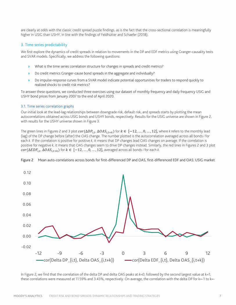
Our initial look at the lead-lag relationships between downgrade risk, default risk, and spreads starts by plotting the mean autocorrelations obtained across USIG bonds and USHY bonds, respectively. Results for the USIG universe are shown in Figure 2, with results for the USHY universe shown in Figure 3.
The green lines in Figures 2 and 3 plot 𝑐𝑐𝑐𝑐𝑐𝑐(∆𝐷𝐷𝐷𝐷𝑖𝑖,𝑡𝑡 , ∆𝑂𝑂𝑂𝑂𝑂𝑂𝑖𝑖,𝑡𝑡+𝑘𝑘) for 𝑘𝑘 ∈ [−12, … , 0, … , 12], where k refers to the monthly lead (lag) of the DP change before (after) the OAS change. The number plotted is the autocorrelation averaged across all bonds i for each k. If the correlation is positive for positive k, it means that DP changes lead OAS changes on average. If the correlation is positive for negative k, it means that OAS changes seem to drive DP changes instead. Similarly, the red lines in Figures 2 and 3 plot 𝑐𝑐𝑐𝑐𝑐𝑐(∆𝐸𝐸𝐷𝐷𝐹𝐹𝑖𝑖,𝑡𝑡 , ∆𝑂𝑂𝑂𝑂𝑂𝑂𝑖𝑖,𝑡𝑡+𝑘𝑘) for 𝑘𝑘 ∈ [−12, … , 0, … , 12], averaged across all bonds i for each k.
Figure 2 Mean auto-correlations across bonds for first-differenced DP and OAS, first-differenced EDF and OAS: USIG market
In Figure 2, we find that the correlation of the delta DP and delta OAS peaks at k=0, followed by the second largest value at k=1; these correlations were measured at 11.59% and 3.43%, respectively. On average, the correlation with the delta DP for k=-1 to k=-
-0.02
0.00
0.02
0.04
0.06
0.08
0.10
0.12
-12 -9 -6 -3 0 3 6 9 12cor(Delta DP_{i,t}, Delta OAS_{i,t+k}) cor(Delta EDF_{i,t}, Delta OAS_{i,t+k})
MOODY’S ANALYTICS CREDIT RISK AND BOND SPREADS: DYNAMIC RELATIONSHIPS AND TRADING STRATEGIES 8
7 is 0.43% while it is 1.08% for k=+1 to k=+7. This shows that there is more correlation—more than double—between DP changes and future OAS changes than there is between OAS changes and future DP changes.
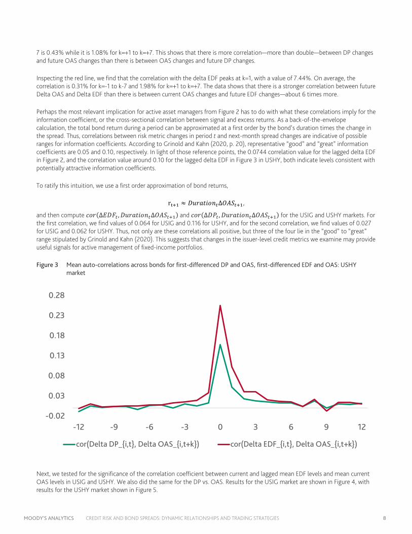
Inspecting the red line, we find that the correlation with the delta EDF peaks at k=1, with a value of 7.44%. On average, the correlation is 0.31% for k=-1 to k-7 and 1.98% for k=+1 to k=+7. The data shows that there is a stronger correlation between future Delta OAS and Delta EDF than there is between current OAS changes and future EDF changes—about 6 times more.
Perhaps the most relevant implication for active asset managers from Figure 2 has to do with what these correlations imply for the information coefficient, or the cross-sectional correlation between signal and excess returns. As a back-of-the-envelope calculation, the total bond return during a period can be approximated at a first order by the bond’s duration times the change in the spread. Thus, correlations between risk metric changes in period t and next-month spread changes are indicative of possible ranges for information coefficients. According to Grinold and Kahn (2020, p. 20), representative “good” and “great” information coefficients are 0.05 and 0.10, respectively. In light of those reference points, the 0.0744 correlation value for the lagged delta EDF in Figure 2, and the correlation value around 0.10 for the lagged delta EDF in Figure 3 in USHY, both indicate levels consistent with potentially attractive information coefficients.
To ratify this intuition, we use a first order approximation of bond returns,
rt+1 ≈ 𝐷𝐷𝐷𝐷𝑐𝑐𝐷𝐷𝐷𝐷𝐷𝐷𝑐𝑐𝑛𝑛𝑡𝑡Δ𝑂𝑂𝑂𝑂𝑂𝑂𝑡𝑡+1,
and then compute 𝑐𝑐𝑐𝑐𝑐𝑐(Δ𝐸𝐸𝐷𝐷𝐹𝐹𝑡𝑡 ,𝐷𝐷𝐷𝐷𝑐𝑐𝐷𝐷𝐷𝐷𝐷𝐷𝑐𝑐𝑛𝑛𝑡𝑡Δ𝑂𝑂𝑂𝑂𝑂𝑂𝑡𝑡+1) and 𝑐𝑐𝑐𝑐𝑐𝑐(Δ𝐷𝐷𝐷𝐷𝑡𝑡 ,𝐷𝐷𝐷𝐷𝑐𝑐𝐷𝐷𝐷𝐷𝐷𝐷𝑐𝑐𝑛𝑛𝑡𝑡Δ𝑂𝑂𝑂𝑂𝑂𝑂𝑡𝑡+1) for the USIG and USHY markets. For the first correlation, we find values of 0.064 for USIG and 0.116 for USHY, and for the second correlation, we find values of 0.027 for USIG and 0.062 for USHY. Thus, not only are these correlations all positive, but three of the four lie in the “good” to “great” range stipulated by Grinold and Kahn (2020). This suggests that changes in the issuer-level credit metrics we examine may provide useful signals for active management of fixed-income portfolios.
Figure 3 Mean auto-correlations across bonds for first-differenced DP and OAS, first-differenced EDF and OAS: USHY market
Next, we tested for the significance of the correlation coefficient between current and lagged mean EDF levels and mean current OAS levels in USIG and USHY. We also did the same for the DP vs. OAS. Results for the USIG market are shown in Figure 4, with results for the USHY market shown in Figure 5.
-0.02
0.03
0.08
0.13
0.18
0.23
0.28
-12 -9 -6 -3 0 3 6 9 12
cor(Delta DP_{i,t}, Delta OAS_{i,t+k}) cor(Delta EDF_{i,t}, Delta OAS_{i,t+k})
MOODY’S ANALYTICS CREDIT RISK AND BOND SPREADS: DYNAMIC RELATIONSHIPS AND TRADING STRATEGIES 9
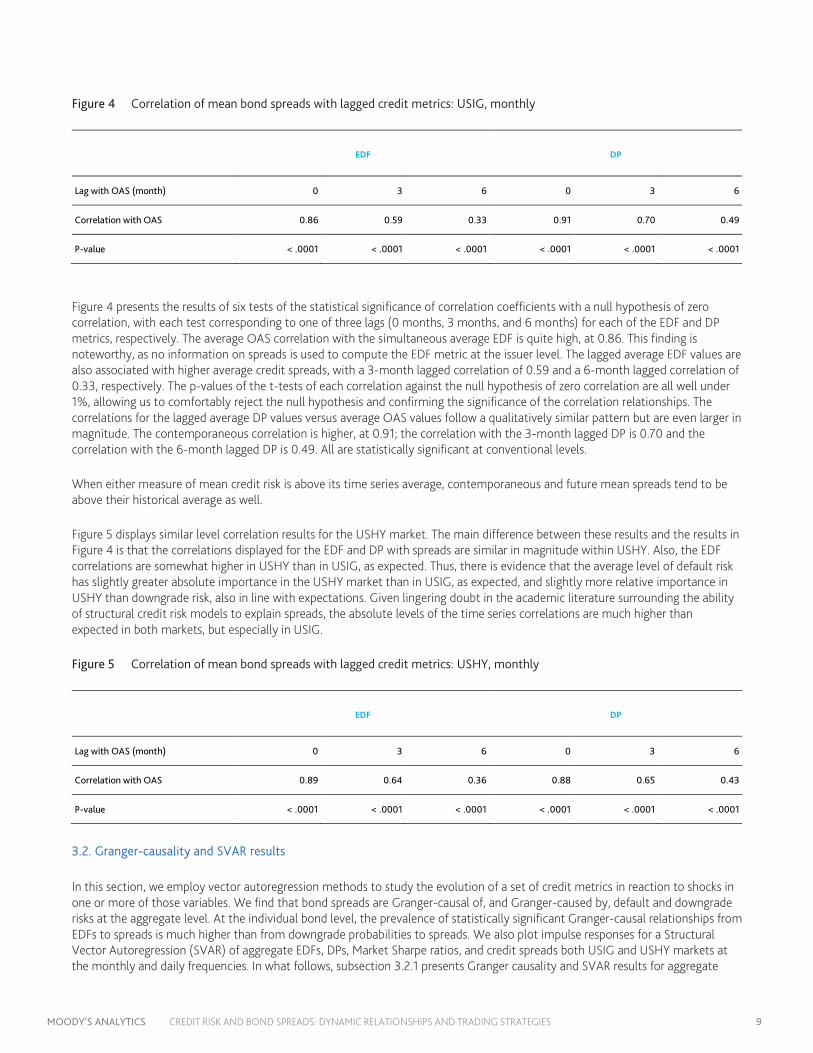
Figure 4 Correlation of mean bond spreads with lagged credit metrics: USIG, monthly
EDF DP
Lag with OAS (month) 0 3 6 0 3 6
Correlation with OAS 0.86 0.59 0.33 0.91 0.70 0.49
P-value < .0001 < .0001 < .0001 < .0001 < .0001 < .0001
Figure 4 presents the results of six tests of the statistical significance of correlation coefficients with a null hypothesis of zero correlation, with each test corresponding to one of three lags (0 months, 3 months, and 6 months) for each of the EDF and DP metrics, respectively. The average OAS correlation with the simultaneous average EDF is quite high, at 0.86. This finding is noteworthy, as no information on spreads is used to compute the EDF metric at the issuer level. The lagged average EDF values are also associated with higher average credit spreads, with a 3-month lagged correlation of 0.59 and a 6-month lagged correlation of 0.33, respectively. The p-values of the t-tests of each correlation against the null hypothesis of zero correlation are all well under 1%, allowing us to comfortably reject the null hypothesis and confirming the significance of the correlation relationships. The correlations for the lagged average DP values versus average OAS values follow a qualitatively similar pattern but are even larger in magnitude. The contemporaneous correlation is higher, at 0.91; the correlation with the 3-month lagged DP is 0.70 and the correlation with the 6-month lagged DP is 0.49. All are statistically significant at conventional levels.
When either measure of mean credit risk is above its time series average, contemporaneous and future mean spreads tend to be above their historical average as well.
Figure 5 displays similar level correlation results for the USHY market. The main difference between these results and the results in Figure 4 is that the correlations displayed for the EDF and DP with spreads are similar in magnitude within USHY. Also, the EDF correlations are somewhat higher in USHY than in USIG, as expected. Thus, there is evidence that the average level of default risk has slightly greater absolute importance in the USHY market than in USIG, as expected, and slightly more relative importance in USHY than downgrade risk, also in line with expectations. Given lingering doubt in the academic literature surrounding the ability of structural credit risk models to explain spreads, the absolute levels of the time series correlations are much higher than expected in both markets, but especially in USIG.
Figure 5 Correlation of mean bond spreads with lagged credit metrics: USHY, monthly
EDF DP
Lag with OAS (month) 0 3 6 0 3 6
Correlation with OAS 0.89 0.64 0.36 0.88 0.65 0.43
P-value < .0001 < .0001 < .0001 < .0001 < .0001 < .0001
3.2. Granger-causality and SVAR results
In this section, we employ vector autoregression methods to study the evolution of a set of credit metrics in reaction to shocks in one or more of those variables. We find that bond spreads are Granger-causal of, and Granger-caused by, default and downgrade risks at the aggregate level. At the individual bond level, the prevalence of statistically significant Granger-causal relationships from EDFs to spreads is much higher than from downgrade probabilities to spreads. We also plot impulse responses for a Structural Vector Autoregression (SVAR) of aggregate EDFs, DPs, Market Sharpe ratios, and credit spreads both USIG and USHY markets at the monthly and daily frequencies. In what follows, subsection 3.2.1 presents Granger causality and SVAR results for aggregate
MOODY’S ANALYTICS CREDIT RISK AND BOND SPREADS: DYNAMIC RELATIONSHIPS AND TRADING STRATEGIES 10
spread data (that is, average spreads), and subsection 3.2.2 focuses on summarizing Granger causality test results for individual bonds at the daily frequency.
3.2.1. Aggregate spreads and credit metrics: Granger-causality and SVAR results
Granger-causality is a statistical notion of time series causality proposed by Clive Granger (1969). The reduced-form VAR model that forms the Granger causality test is as follows:
𝑦𝑦𝑡𝑡 = 𝑐𝑐 + 𝐷𝐷1 𝑦𝑦𝑡𝑡−1 + ⋯+ 𝐷𝐷𝑝𝑝 𝑦𝑦𝑡𝑡−𝑝𝑝 + 𝑏𝑏1 𝑥𝑥𝑡𝑡−1 + ⋯+ 𝑏𝑏𝑝𝑝 𝑥𝑥𝑡𝑡−𝑞𝑞 + 𝑒𝑒𝑡𝑡
In the above equation, p and q are lag lengths for the variables 𝑦𝑦𝑡𝑡 and 𝑥𝑥𝑡𝑡 , respectively, and the Granger-causality test is an F-test of the joint significance of the coefficients 𝑏𝑏1 , … , 𝑏𝑏𝑝𝑝 under the null hypothesis that they are all equal to zero. We report the p-values of a series of bivariate Granger-causality tests of mean spreads paired with each of the mean EDF metric, the mean DP, and the market Sharpe ratio (MSR). We display results for USIG first, for monthly and daily frequencies, and then results for USHY.
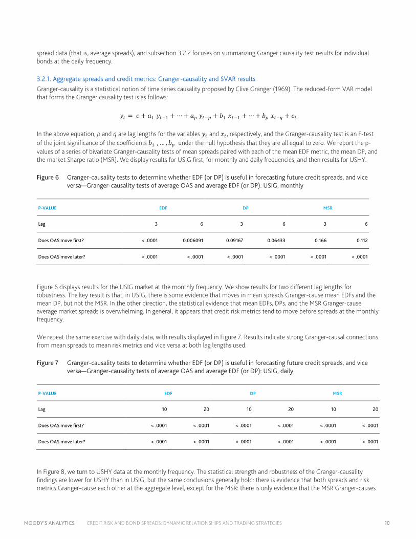
Figure 6 Granger-causality tests to determine whether EDF (or DP) is useful in forecasting future credit spreads, and vice versa—Granger-causality tests of average OAS and average EDF (or DP): USIG, monthly
P-VALUE EDF DP MSR
Lag 3 6 3 6 3 6
Does OAS move first? < .0001 0.006091 0.09167 0.06433 0.166 0.112
Does OAS move later? < .0001 < .0001 < .0001 < .0001 < .0001 < .0001
Figure 6 displays results for the USIG market at the monthly frequency. We show results for two different lag lengths for robustness. The key result is that, in USIG, there is some evidence that moves in mean spreads Granger-cause mean EDFs and the mean DP, but not the MSR. In the other direction, the statistical evidence that mean EDFs, DPs, and the MSR Granger-cause average market spreads is overwhelming. In general, it appears that credit risk metrics tend to move before spreads at the monthly frequency.
We repeat the same exercise with daily data, with results displayed in Figure 7. Results indicate strong Granger-causal connections from mean spreads to mean risk metrics and vice versa at both lag lengths used.
Figure 7 Granger-causality tests to determine whether EDF (or DP) is useful in forecasting future credit spreads, and vice versa—Granger-causality tests of average OAS and average EDF (or DP): USIG, daily
P-VALUE EDF DP MSR
Lag 10 20 10 20 10 20
Does OAS move first? < .0001 < .0001 < .0001 < .0001 < .0001 < .0001
Does OAS move later? < .0001 < .0001 < .0001 < .0001 < .0001 < .0001
In Figure 8, we turn to USHY data at the monthly frequency. The statistical strength and robustness of the Granger-causality findings are lower for USHY than in USIG, but the same conclusions generally hold: there is evidence that both spreads and risk metrics Granger-cause each other at the aggregate level, except for the MSR: there is only evidence that the MSR Granger-causes
MOODY’S ANALYTICS CREDIT RISK AND BOND SPREADS: DYNAMIC RELATIONSHIPS AND TRADING STRATEGIES 11
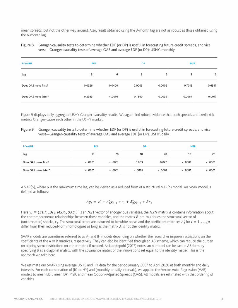
mean spreads, but not the other way around. Also, result obtained using the 3-month lag are not as robust as those obtained using the 6-month lag.
Figure 8 Granger-causality tests to determine whether EDF (or DP) is useful in forecasting future credit spreads, and vice versa—Granger-causality tests of average OAS and average EDF (or DP): USHY, monthly
P-VALUE EDF DP MSR
Lag 3 6 3 6 3 6
Does OAS move first? 0.0226 0.0400 0.0005 0.0006 0.7012 0.6547
Does OAS move later? 0.2283 < .0001 0.1840 0.0039 0.0064 0.0017
Figure 9 displays daily aggregate USHY Granger-causality results. We again find robust evidence that both spreads and credit risk metrics Granger-cause each other in the USHY market.
Figure 9 Granger-causality tests to determine whether EDF (or DP) is useful in forecasting future credit spreads, and vice versa—Granger-causality tests of average OAS and average EDF (or DP): USHY, daily
P-VALUE EDF DP MSR
Lag 10 20 10 20 10 20
Does OAS move first? < .0001 < .0001 0.003 0.022 < .0001 < .0001
Does OAS move later? < .0001 < .0001 < .0001 < .0001 < .0001 < .0001
A VAR(ρ), where ρ is the maximum time lag, can be viewed as a reduced form of a structural VAR(p) model. An SVAR model is defined as follows:
𝑂𝑂𝑦𝑦𝑡𝑡 = 𝑐𝑐∗ + 𝑂𝑂1∗𝑦𝑦𝑡𝑡−1 + ⋯+ 𝑂𝑂𝑝𝑝∗ 𝑦𝑦𝑡𝑡−𝑝𝑝 + 𝐵𝐵𝜖𝜖𝑡𝑡
Here 𝑦𝑦𝑡𝑡 ≡ (𝐸𝐸𝐷𝐷𝐹𝐹𝑡𝑡 ,𝐷𝐷𝐷𝐷𝑡𝑡 ,𝑀𝑀𝑂𝑂𝑀𝑀𝑡𝑡 ,𝑂𝑂𝑂𝑂𝑂𝑂𝑡𝑡)′ is an 𝑁𝑁𝑥𝑥1 vector of endogenous variables, the 𝑁𝑁𝑥𝑥𝑁𝑁 matrix 𝑂𝑂 contains information about the contemporaneous relationships between those variables, and the matrix 𝐵𝐵 pre-multiplies the structural vector of (uncorrelated) shocks, 𝜖𝜖𝑡𝑡. The structural errors are assumed to be white noise, and the coefficient matrices 𝑂𝑂𝑡𝑡𝑖𝑖 for 𝐷𝐷 = 1, . … ,𝜌𝜌 differ from their reduced-form homologues as long as the matrix 𝑂𝑂 is not the identity matrix.
SVAR models are sometimes referred to as A- and B- models depending on whether the researcher imposes restrictions on the coefficients of the A or B matrices, respectively. They can also be identified through an AB scheme, which can reduce the burden on placing some restrictions on either matrix if needed. As Luetkepohl (2017) notes, an A-model can be cast in AB form by specifying B as a diagonal matrix, with the covariance matrix of the innovations set equal to the identity matrix. This is the approach we take here.
We estimate our SVAR using average US IG and HY data for the period January 2007 to April 2020 at both monthly and daily intervals. For each combination of (IG or HY) and (monthly or daily intervals), we applied the Vector Auto-Regression (VAR) models to mean EDF, mean DP, MSR, and mean Option-Adjusted Spreads (OAS). All models are estimated with that ordering of variables.
MOODY’S ANALYTICS CREDIT RISK AND BOND SPREADS: DYNAMIC RELATIONSHIPS AND TRADING STRATEGIES 12
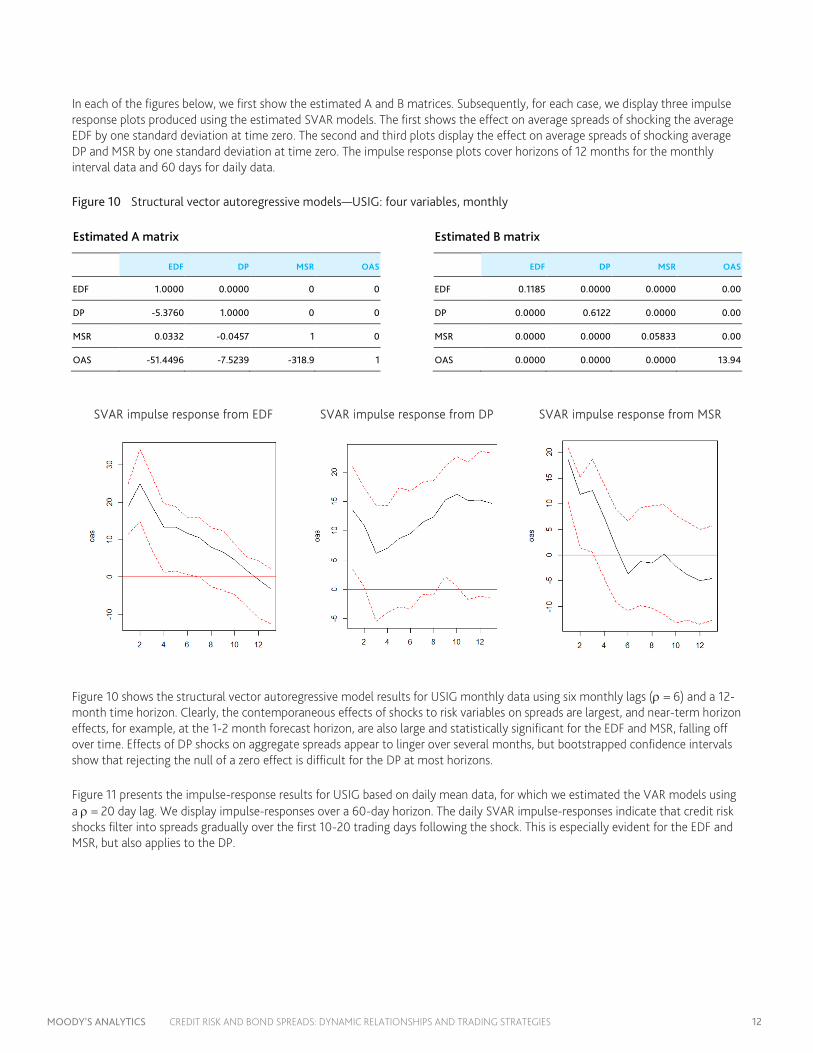
In each of the figures below, we first show the estimated A and B matrices. Subsequently, for each case, we display three impulse response plots produced using the estimated SVAR models. The first shows the effect on average spreads of shocking the average EDF by one standard deviation at time zero. The second and third plots display the effect on average spreads of shocking average DP and MSR by one standard deviation at time zero. The impulse response plots cover horizons of 12 months for the monthly interval data and 60 days for daily data.
Figure 10 Structural vector autoregressive models—USIG: four variables, monthly
Estimated A matrix Estimated B matrix
EDF DP MSR OAS EDF DP MSR OAS
EDF 1.0000 0.0000 0 0 EDF 0.1185 0.0000 0.0000 0.00
DP -5.3760 1.0000 0 0 DP 0.0000 0.6122 0.0000 0.00
MSR 0.0332 -0.0457 1 0 MSR 0.0000 0.0000 0.05833 0.00
OAS -51.4496 -7.5239 -318.9 1 OAS 0.0000 0.0000 0.0000 13.94
SVAR impulse response from EDF SVAR impulse response from DP SVAR impulse response from MSR
Figure 10 shows the structural vector autoregressive model results for USIG monthly data using six monthly lags (ρ = 6) and a 12-month time horizon. Clearly, the contemporaneous effects of shocks to risk variables on spreads are largest, and near-term horizon effects, for example, at the 1-2 month forecast horizon, are also large and statistically significant for the EDF and MSR, falling off over time. Effects of DP shocks on aggregate spreads appear to linger over several months, but bootstrapped confidence intervals show that rejecting the null of a zero effect is difficult for the DP at most horizons.
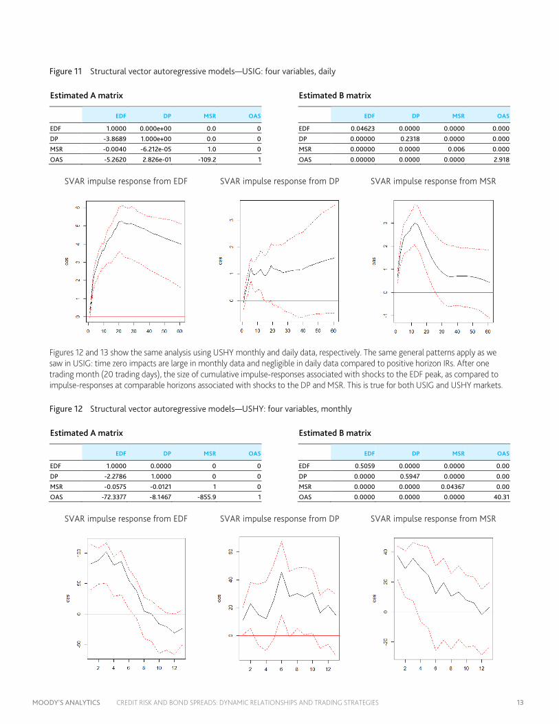
Figure 11 presents the impulse-response results for USIG based on daily mean data, for which we estimated the VAR models using a ρ = 20 day lag. We display impulse-responses over a 60-day horizon. The daily SVAR impulse-responses indicate that credit risk shocks filter into spreads gradually over the first 10-20 trading days following the shock. This is especially evident for the EDF and MSR, but also applies to the DP.
MOODY’S ANALYTICS CREDIT RISK AND BOND SPREADS: DYNAMIC RELATIONSHIPS AND TRADING STRATEGIES 13
Figure 11 Structural vector autoregressive models—USIG: four variables, daily
Estimated A matrix Estimated B matrix
EDF DP MSR OAS EDF DP MSR OAS
EDF 1.0000 0.000e+00 0.0 0 EDF 0.04623 0.0000 0.0000 0.000 DP -3.8689 1.000e+00 0.0 0 DP 0.00000 0.2318 0.0000 0.000 MSR -0.0040 -6.212e-05 1.0 0 MSR 0.00000 0.0000 0.006 0.000
OAS -5.2620 2.826e-01 -109.2 1 OAS 0.00000 0.0000 0.0000 2.918
SVAR impulse response from EDF SVAR impulse response from DP SVAR impulse response from MSR
Figures 12 and 13 show the same analysis using USHY monthly and daily data, respectively. The same general patterns apply as we saw in USIG: time zero impacts are large in monthly data and negligible in daily data compared to positive horizon IRs. After one trading month (20 trading days), the size of cumulative impulse-responses associated with shocks to the EDF peak, as compared to impulse-responses at comparable horizons associated with shocks to the DP and MSR. This is true for both USIG and USHY markets.
Figure 12 Structural vector autoregressive models—USHY: four variables, monthly
Estimated A matrix Estimated B matrix
EDF DP MSR OAS EDF DP MSR OAS
EDF 1.0000 0.0000 0 0 EDF 0.5059 0.0000 0.0000 0.00
DP -2.2786 1.0000 0 0 DP 0.0000 0.5947 0.0000 0.00 MSR -0.0575 -0.0121 1 0 MSR 0.0000 0.0000 0.04367 0.00 OAS -72.3377 -8.1467 -855.9 1 OAS 0.0000 0.0000 0.0000 40.31
SVAR impulse response from EDF SVAR impulse response from DP SVAR impulse response from MSR
MOODY’S ANALYTICS CREDIT RISK AND BOND SPREADS: DYNAMIC RELATIONSHIPS AND TRADING STRATEGIES 14
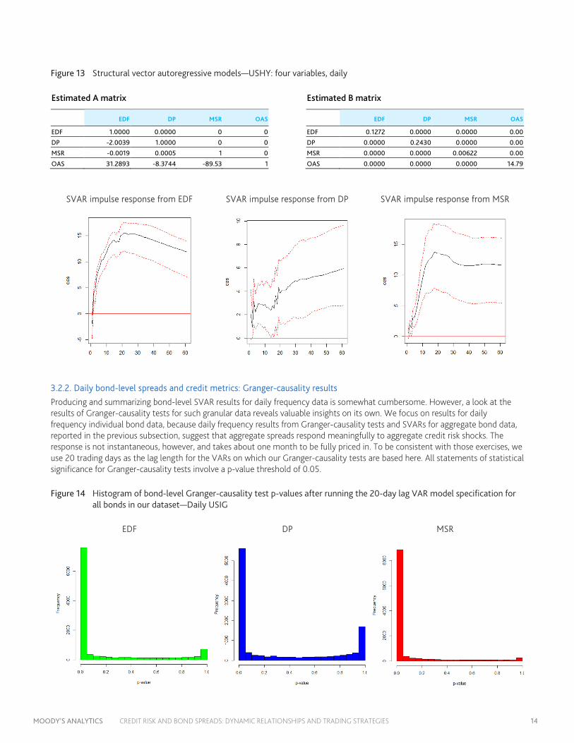
Figure 13 Structural vector autoregressive models—USHY: four variables, daily
Estimated A matrix Estimated B matrix
EDF DP MSR OAS EDF DP MSR OAS
EDF 1.0000 0.0000 0 0 EDF 0.1272 0.0000 0.0000 0.00 DP -2.0039 1.0000 0 0 DP 0.0000 0.2430 0.0000 0.00 MSR -0.0019 0.0005 1 0 MSR 0.0000 0.0000 0.00622 0.00
OAS 31.2893 -8.3744 -89.53 1 OAS 0.0000 0.0000 0.0000 14.79
SVAR impulse response from EDF SVAR impulse response from DP SVAR impulse response from MSR
3.2.2. Daily bond-level spreads and credit metrics: Granger-causality results
Producing and summarizing bond-level SVAR results for daily frequency data is somewhat cumbersome. However, a look at the results of Granger-causality tests for such granular data reveals valuable insights on its own. We focus on results for daily frequency individual bond data, because daily frequency results from Granger-causality tests and SVARs for aggregate bond data, reported in the previous subsection, suggest that aggregate spreads respond meaningfully to aggregate credit risk shocks. The response is not instantaneous, however, and takes about one month to be fully priced in. To be consistent with those exercises, we use 20 trading days as the lag length for the VARs on which our Granger-causality tests are based here. All statements of statistical significance for Granger-causality tests involve a p-value threshold of 0.05.
Figure 14 Histogram of bond-level Granger-causality test p-values after running the 20-day lag VAR model specification for all bonds in our dataset—Daily USIG
EDF DP MSR
MOODY’S ANALYTICS CREDIT RISK AND BOND SPREADS: DYNAMIC RELATIONSHIPS AND TRADING STRATEGIES 15
Our results are as follows. In daily bond data for the USIG market, we find that the fraction of bonds for which credit metrics Granger-cause, the spread is 68% for the EDF, 50% for the DP, and 78% for the MSR. Histograms of p-values for the Granger-causality test statistics across bonds in USIG are shown in Figure 14, with the EDF on the left, the DP in the middle, and results for the MSR on the right. Before running the GC tests, we screened out bonds with less than 98% of trading days of available (non-missing) spreads, as well as all bonds that exhibited a lack of variation in spreads and bonds with less than six months of data.
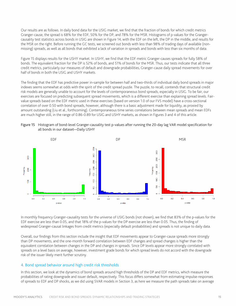
Figure 15 displays results for the USHY market. In USHY, we find that the EDF metric Granger-causes spreads for fully 58% of bonds. The equivalent fraction for the DP is 52% of bonds, and 51% of bonds for the MSR. Thus, our tests indicate that all three credit metrics, particularly our measures of default and downgrade probabilities, Granger-cause daily spread movements for over half of bonds in both the USIG and USHY markets.
The finding that the EDF has predictive power in-sample for between half and two-thirds of individual daily bond spreads in major indexes seems somewhat at odds with the spirit of the credit spread puzzle. The puzzle, to recall, contends that structural credit risk models are generally unable to account for the levels of contemporaneous bond spreads, especially in USIG. To be fair, our exercises are focused on predicting subsequent spread movements, which is a different exercise than explaining spread levels. Fair-value spreads based on the EDF metric used in these exercises (based on version 1.0 of our FVS model) have a cross-sectional correlation of over 0.50 with bond spreads, however, although there is a basic adjustment made for liquidity, as proxied by amount outstanding (Liu et al., forthcoming). Contemporaneous time series correlations between mean spreads and mean EDFs are much higher still, in the range of 0.86-0.89 for USIG and USHY markets, as shown in Figures 3 and 4 of this article.
Figure 15 Histogram of bond-level Granger-causality test p-values after running the 20-day lag VAR model specification for all bonds in our dataset—Daily USHY
EDF DP MSR
In monthly frequency Granger-causality tests for the universe of USIG bonds (not shown), we find that 83% of the p-values for the EDF exercise are less than 0.05, and that 18% of the p-values for the DP exercise are less than 0.05. Thus, the finding of widespread Granger-causal linkages from credit metrics (especially default probabilities) and spreads is not unique to daily data.
Overall, our findings from this section include the insight that EDF movements appear to Granger-cause spreads more strongly than DP movements, and the one-month forward correlation between EDF changes and spread changes is higher than the equivalent correlation between changes in the DP and changes in spreads. Since DP levels appear more strongly correlated with spreads on a level basis on average, however, investment grade bonds for which spread levels do not accord with the downgrade risk of the issuer likely merit further scrutiny.
4. Bond spread behavior around high credit risk thresholds
In this section, we look at the dynamics of bond spreads around high thresholds of the DP and EDF metrics, which measure the probabilities of rating downgrade and issuer default, respectively. This focus differs somewhat from estimating impulse-responses of spreads to EDF and DP shocks, as we did using SVAR models in Section 3, as here we measure the path spreads take on average
MOODY’S ANALYTICS CREDIT RISK AND BOND SPREADS: DYNAMIC RELATIONSHIPS AND TRADING STRATEGIES 16
following—and just prior to—high-risk threshold exceedances. This exercise therefore lies at the intersection of interests of credit risk managers and quantitative portfolio managers or traders looking to take reasonable positions in particular bonds.
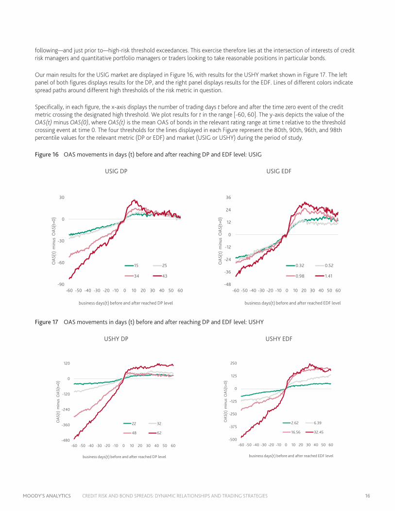
Our main results for the USIG market are displayed in Figure 16, with results for the USHY market shown in Figure 17. The left panel of both figures displays results for the DP, and the right panel displays results for the EDF. Lines of different colors indicate spread paths around different high thresholds of the risk metric in question.
Specifically, in each figure, the x-axis displays the number of trading days t before and after the time zero event of the credit metric crossing the designated high threshold. We plot results for t in the range [-60, 60]. The y-axis depicts the value of the OAS(t) minus OAS(0), where OAS(t) is the mean OAS of bonds in the relevant rating range at time t relative to the threshold crossing event at time 0. The four thresholds for the lines displayed in each Figure represent the 80th, 90th, 96th, and 98th percentile values for the relevant metric (DP or EDF) and market (USIG or USHY) during the period of study.
Figure 16 OAS movements in days (t) before and after reaching DP and EDF level: USIG
USIG DP USIG EDF
Figure 17 OAS movements in days (t) before and after reaching DP and EDF level: USHY
USHY DP USHY EDF
-90
-60
-30
0
30
-60 -50 -40 -30 -20 -10 0 10 20 30 40 50 60
OAS
(t)
min
us O
AS(t
=0)
business days(t) before and after reached DP level
15 25
34 43
-48
-36
-24
-12
0
12
24
36
-60 -50 -40 -30 -20 -10 0 10 20 30 40 50 60
OAS
(t)
min
us O
AS(t
=0)
business days(t) before and after reached EDF level
0.32 0.52
0.98 1.41
-480
-360
-240
-120
0
120
-60 -50 -40 -30 -20 -10 0 10 20 30 40 50 60
OAS
(t)
min
us O
AS(t
=0)
business days(t) before and after reached DP level
22 32
48 62
-500
-375
-250
-125
0
125
250
-60 -50 -40 -30 -20 -10 0 10 20 30 40 50 60
OAS
(t)
min
us O
AS(t
=0)
business days(t) before and after reached EDF level
2.62 6.39
16.56 32.45

MOODY’S ANALYTICS CREDIT RISK AND BOND SPREADS: DYNAMIC RELATIONSHIPS AND TRADING STRATEGIES 17
Exceedance of EDF thresholds in the 80-98th percentile range in USIG is associated with a rise in spreads of 13-30 bps, respectively, over the next 20 trading days, and a rise in spreads of 33-182 bps over the same period in USHY. For the DP, the rise in spreads over 20 trading days equates to 6-15 bps in USIG and 24-93 bps in USHY for exceedance of DP thresholds in the 80-98th percentile range. Across bonds, average monthly OAS time series standard deviations are 60 bps in USIG and 242 bps in USHY. Thus, spread changes following high EDF exceedances translate into 20-50% of the average monthly OAS standard deviation in USIG and 14-75% of the monthly spread standard deviation in USHY. The equivalent percentages for the DP are 10-25% in USIG and 10-38% in USHY. These magnitudes are highly material in both fixed-income markets, and as expected, larger in USHY. At the individual bond level, exceeding high levels of default and downgrade risk translates into large increases in spreads over the next month.
5. Credit risk and the cross-section of bond returns
Having examined time series spread behavior conditional on credit risk metrics, and around high thresholds for default and downgrade probabilities (time series predictability), we now look at whether misalignment of spreads with fair value implied by those credit metrics helps to explain the cross-section of next-month bond returns (relative return predictability). We find that it does.
5.1. A few simple pricing models for bond-level OAS
The basic premise of many statistical arbitrage strategies, including those studied here, is that deviations from reasonable estimates of fair value will revert to zero on average over time. The ability to gain exposure to such movements can generate attractive risk-adjusted returns.
In line with these ideas, we study three types of fair value models for bond spreads: those that model spreads as a function of bond spread duration, agency rating, and issuer industry (Basic quant models), those that model spreads as a function of CreditEdge metrics, in particular some combination of the Fair Value Spread (FVS), Expected Default Frequency (EDF), and Deterioration Probability (DP) (CE quant models) and those that incorporate both sets of factors (Combined quant models).
Our basic statistical arbitrage strategy involves running cross-sectional spread pricing regressions at the monthly frequency, extracting the residuals from those regressions, bucketing the index (USIG or USHY) into five duration buckets on each date, and sorting by model residual within each bucket. Within duration buckets, bonds are grouped into quintile portfolios by model residual. Finally, we pool bonds in the relevant residual quintile portfolio across duration buckets and apply equal weights to form five portfolios by residual quintile. The step of sorting within duration bucket and recombining is meant to ensure that the duration profile of each residual quintile portfolio resembles that of the index from which the underlying bonds are selected. This helps ensure that unintended exposure to duration risk does not inadvertently affect our results.
We now describe our three cross-sectional regressions in more detail. Each can be viewed as a restriction of the following model:
𝑂𝑂𝑂𝑂𝑂𝑂𝑖𝑖𝑡𝑡 = 𝛼𝛼 + 𝛽𝛽𝐵𝐵𝐵𝐵𝐵𝐵𝑖𝑖𝐵𝐵 ,𝑡𝑡′ �⃑�𝑋𝐵𝐵𝐵𝐵𝐵𝐵𝑖𝑖𝐵𝐵,𝑖𝑖𝑡𝑡 + 𝛽𝛽𝐶𝐶𝐶𝐶,𝑡𝑡
′ �⃑�𝑋𝐶𝐶𝐶𝐶,𝑖𝑖𝑡𝑡 + 𝜀𝜀𝑖𝑖𝑡𝑡
Here �⃑�𝑋𝐵𝐵𝐵𝐵𝐵𝐵𝑖𝑖𝐵𝐵 ,𝑖𝑖𝑡𝑡 ≡ (𝐷𝐷𝐷𝐷𝑐𝑐𝐷𝐷𝐷𝐷𝐷𝐷𝑐𝑐𝑛𝑛𝑖𝑖𝑡𝑡 ,𝑀𝑀𝐷𝐷𝐷𝐷𝐷𝐷𝑛𝑛𝑅𝑅𝑖𝑖𝑡𝑡 , 𝐼𝐼𝑛𝑛𝐼𝐼𝐷𝐷𝐼𝐼𝐷𝐷𝑐𝑐𝑦𝑦�������������������⃑ 𝑖𝑖𝑡𝑡)′, where 𝐷𝐷𝐷𝐷𝑐𝑐𝐷𝐷𝐷𝐷𝐷𝐷𝑐𝑐𝑛𝑛𝑖𝑖𝑡𝑡 is the spread duration of bond i at time t, 𝑀𝑀𝐷𝐷𝐷𝐷𝐷𝐷𝑛𝑛𝑅𝑅𝑖𝑖𝑡𝑡 is the issuer rating, and 𝐼𝐼𝑛𝑛𝐼𝐼𝐷𝐷𝐼𝐼𝐷𝐷𝑐𝑐𝑦𝑦�������������������⃑ 𝑖𝑖𝑡𝑡 is a vector of 12 industry dummy variables that encode which of the 13 industries the issue belongs to. As usual, the effect of the omitted 13th industry is absorbed into the constant term of the regression. The vector �⃑�𝑋𝐶𝐶𝐶𝐶,𝑖𝑖𝑡𝑡 ≡ (𝐸𝐸𝐷𝐷𝐹𝐹𝑖𝑖𝑡𝑡 ,𝐷𝐷𝐷𝐷𝑖𝑖𝑡𝑡 ,𝐹𝐹𝐹𝐹𝑂𝑂𝑖𝑖𝑡𝑡)′, where 𝐸𝐸𝐷𝐷𝐹𝐹𝑖𝑖𝑡𝑡 is the one-year real-world default probability of the issuer, 𝐷𝐷𝐷𝐷𝑖𝑖𝑡𝑡 is the rating downgrade probability, and 𝐹𝐹𝐹𝐹𝑂𝑂𝑖𝑖𝑡𝑡 is the modeled fair-value spread of the bond based on its default risk, sector loss-given-default (LGD) estimate, seniority, and the estimated market Sharpe ratio. At the end of each month, we estimate the parameters of the relevant restriction of the above regression model using OLS, calculate estimates for the bond-level residuals 𝜀𝜀𝚤𝚤𝑡𝑡�, and use those estimated residuals to form quintile portfolios as described above.
The Basic quant model restriction is given by 𝛽𝛽𝐶𝐶𝐶𝐶,𝑡𝑡′ = 0, the CE quant restriction is given by 𝛽𝛽𝐵𝐵𝐵𝐵𝐵𝐵𝑖𝑖𝐵𝐵,𝑡𝑡
′ = 0, and the Combined quant model is given by estimating the unrestricted version of the model equation. In addition, to tease out which of the CE factors matter most, we estimate versions of the CE quant and Combined quant models with each of the seven possible combinations of the three CE variables.
MOODY’S ANALYTICS CREDIT RISK AND BOND SPREADS: DYNAMIC RELATIONSHIPS AND TRADING STRATEGIES 18
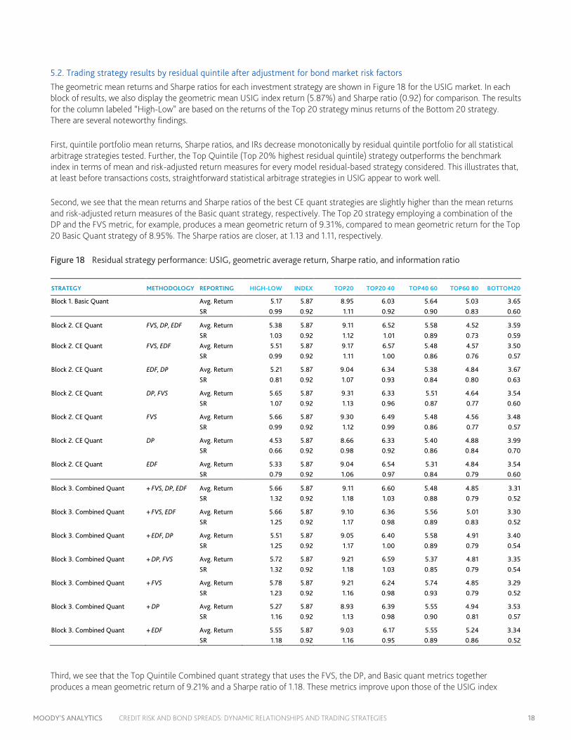
5.2. Trading strategy results by residual quintile after adjustment for bond market risk factors
The geometric mean returns and Sharpe ratios for each investment strategy are shown in Figure 18 for the USIG market. In each block of results, we also display the geometric mean USIG index return (5.87%) and Sharpe ratio (0.92) for comparison. The results for the column labeled “High-Low” are based on the returns of the Top 20 strategy minus returns of the Bottom 20 strategy. There are several noteworthy findings.
First, quintile portfolio mean returns, Sharpe ratios, and IRs decrease monotonically by residual quintile portfolio for all statistical arbitrage strategies tested. Further, the Top Quintile (Top 20% highest residual quintile) strategy outperforms the benchmark index in terms of mean and risk-adjusted return measures for every model residual-based strategy considered. This illustrates that, at least before transactions costs, straightforward statistical arbitrage strategies in USIG appear to work well.
Second, we see that the mean returns and Sharpe ratios of the best CE quant strategies are slightly higher than the mean returns and risk-adjusted return measures of the Basic quant strategy, respectively. The Top 20 strategy employing a combination of the DP and the FVS metric, for example, produces a mean geometric return of 9.31%, compared to mean geometric return for the Top 20 Basic Quant strategy of 8.95%. The Sharpe ratios are closer, at 1.13 and 1.11, respectively.
Figure 18 Residual strategy performance: USIG, geometric average return, Sharpe ratio, and information ratio
STRATEGY METHODOLOGY REPORTING HIGH-LOW INDEX TOP20 TOP20 40 TOP40 60 TOP60 80 BOTTOM20
Block 1. Basic Quant Avg. Return 5.17 5.87 8.95 6.03 5.64 5.03 3.65 SR 0.99 0.92 1.11 0.92 0.90 0.83 0.60
Block 2. CE Quant FVS, DP, EDF Avg. Return 5.38 5.87 9.11 6.52 5.58 4.52 3.59 SR 1.03 0.92 1.12 1.01 0.89 0.73 0.59 Block 2. CE Quant FVS, EDF Avg. Return 5.51 5.87 9.17 6.57 5.48 4.57 3.50 SR 0.99 0.92 1.11 1.00 0.86 0.76 0.57
Block 2. CE Quant EDF, DP Avg. Return 5.21 5.87 9.04 6.34 5.38 4.84 3.67 SR 0.81 0.92 1.07 0.93 0.84 0.80 0.63
Block 2. CE Quant DP, FVS Avg. Return 5.65 5.87 9.31 6.33 5.51 4.64 3.54 SR 1.07 0.92 1.13 0.96 0.87 0.77 0.60
Block 2. CE Quant FVS Avg. Return 5.66 5.87 9.30 6.49 5.48 4.56 3.48 SR 0.99 0.92 1.12 0.99 0.86 0.77 0.57
Block 2. CE Quant DP Avg. Return 4.53 5.87 8.66 6.33 5.40 4.88 3.99 SR 0.66 0.92 0.98 0.92 0.86 0.84 0.70
Block 2. CE Quant EDF Avg. Return 5.33 5.87 9.04 6.54 5.31 4.84 3.54 SR 0.79 0.92 1.06 0.97 0.84 0.79 0.60
Block 3. Combined Quant + FVS, DP, EDF Avg. Return 5.66 5.87 9.11 6.60 5.48 4.85 3.31 SR 1.32 0.92 1.18 1.03 0.88 0.79 0.52
Block 3. Combined Quant + FVS, EDF Avg. Return 5.66 5.87 9.10 6.36 5.56 5.01 3.30 SR 1.25 0.92 1.17 0.98 0.89 0.83 0.52
Block 3. Combined Quant + EDF, DP Avg. Return 5.51 5.87 9.05 6.40 5.58 4.91 3.40 SR 1.25 0.92 1.17 1.00 0.89 0.79 0.54
Block 3. Combined Quant + DP, FVS Avg. Return 5.72 5.87 9.21 6.59 5.37 4.81 3.35 SR 1.32 0.92 1.18 1.03 0.85 0.79 0.54
Block 3. Combined Quant + FVS Avg. Return 5.78 5.87 9.21 6.24 5.74 4.85 3.29 SR 1.23 0.92 1.16 0.98 0.93 0.79 0.52
Block 3. Combined Quant + DP Avg. Return 5.27 5.87 8.93 6.39 5.55 4.94 3.53 SR 1.16 0.92 1.13 0.98 0.90 0.81 0.57
Block 3. Combined Quant + EDF Avg. Return 5.55 5.87 9.03 6.17 5.55 5.24 3.34 SR 1.18 0.92 1.16 0.95 0.89 0.86 0.52
Third, we see that the Top Quintile Combined quant strategy that uses the FVS, the DP, and Basic quant metrics together produces a mean geometric return of 9.21% and a Sharpe ratio of 1.18. These metrics improve upon those of the USIG index
MOODY’S ANALYTICS CREDIT RISK AND BOND SPREADS: DYNAMIC RELATIONSHIPS AND TRADING STRATEGIES 19
during the same period by 334 bps annually in the case of mean geometric returns and by 28% in the case of the Sharpe ratio. Even after applying reasonable transaction cost assumptions for USIG, there is clearly meaningful economic value to be extracted using signals from the types of statistical arbitrage credit strategies considered here.
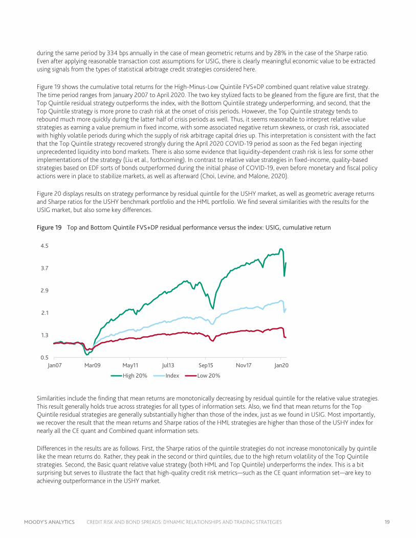
Figure 19 shows the cumulative total returns for the High-Minus-Low Quintile FVS+DP combined quant relative value strategy. The time period ranges from January 2007 to April 2020. The two key stylized facts to be gleaned from the figure are first, that the Top Quintile residual strategy outperforms the index, with the Bottom Quintile strategy underperforming, and second, that the Top Quintile strategy is more prone to crash risk at the onset of crisis periods. However, the Top Quintile strategy tends to rebound much more quickly during the latter half of crisis periods as well. Thus, it seems reasonable to interpret relative value strategies as earning a value premium in fixed income, with some associated negative return skewness, or crash risk, associated with highly volatile periods during which the supply of risk arbitrage capital dries up. This interpretation is consistent with the fact that the Top Quintile strategy recovered strongly during the April 2020 COVID-19 period as soon as the Fed began injecting unprecedented liquidity into bond markets. There is also some evidence that liquidity-dependent crash risk is less for some other implementations of the strategy (Liu et al., forthcoming). In contrast to relative value strategies in fixed-income, quality-based strategies based on EDF sorts of bonds outperformed during the initial phase of COVID-19, even before monetary and fiscal policy actions were in place to stabilize markets, as well as afterward (Choi, Levine, and Malone, 2020).
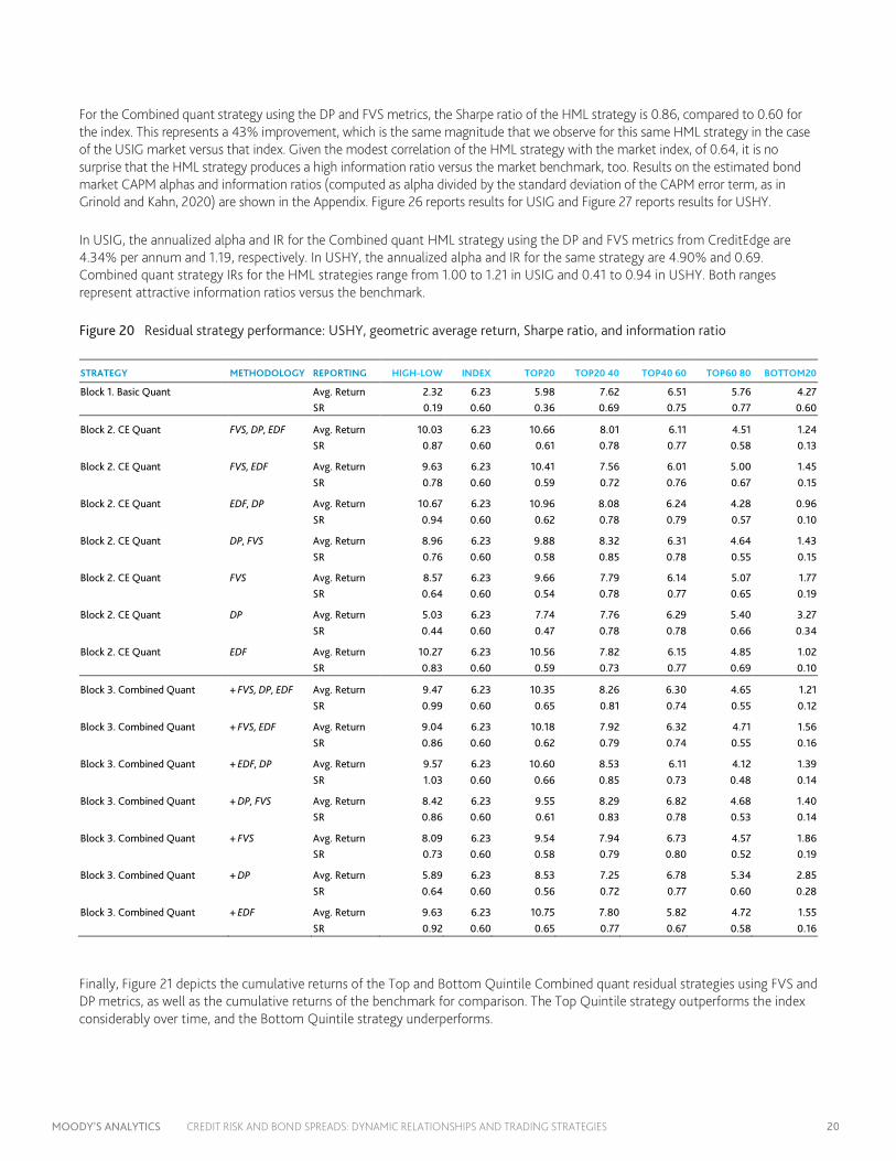
Figure 20 displays results on strategy performance by residual quintile for the USHY market, as well as geometric average returns and Sharpe ratios for the USHY benchmark portfolio and the HML portfolio. We find several similarities with the results for the USIG market, but also some key differences.
Figure 19 Top and Bottom Quintile FVS+DP residual performance versus the index: USIG, cumulative return
Similarities include the finding that mean returns are monotonically decreasing by residual quintile for the relative value strategies. This result generally holds true across strategies for all types of information sets. Also, we find that mean returns for the Top Quintile residual strategies are generally substantially higher than those of the index, just as we found in USIG. Most importantly, we recover the result that the mean returns and Sharpe ratios of the HML strategies are higher than those of the USHY index for nearly all the CE quant and Combined quant information sets.
Differences in the results are as follows. First, the Sharpe ratios of the quintile strategies do not increase monotonically by quintile like the mean returns do. Rather, they peak in the second or third quintiles, due to the high return volatility of the Top Quintile strategies. Second, the Basic quant relative value strategy (both HML and Top Quintile) underperforms the index. This is a bit surprising but serves to illustrate the fact that high-quality credit risk metrics—such as the CE quant information set—are key to achieving outperformance in the USHY market.
0.5
1.3
2.1
2.9
3.7
4.5
Jan07 Mar09 May11 Jul13 Sep15 Nov17 Jan20
High 20% Index Low 20%
MOODY’S ANALYTICS CREDIT RISK AND BOND SPREADS: DYNAMIC RELATIONSHIPS AND TRADING STRATEGIES 20
For the Combined quant strategy using the DP and FVS metrics, the Sharpe ratio of the HML strategy is 0.86, compared to 0.60 for the index. This represents a 43% improvement, which is the same magnitude that we observe for this same HML strategy in the case of the USIG market versus that index. Given the modest correlation of the HML strategy with the market index, of 0.64, it is no surprise that the HML strategy produces a high information ratio versus the market benchmark, too. Results on the estimated bond market CAPM alphas and information ratios (computed as alpha divided by the standard deviation of the CAPM error term, as in Grinold and Kahn, 2020) are shown in the Appendix. Figure 26 reports results for USIG and Figure 27 reports results for USHY.
In USIG, the annualized alpha and IR for the Combined quant HML strategy using the DP and FVS metrics from CreditEdge are 4.34% per annum and 1.19, respectively. In USHY, the annualized alpha and IR for the same strategy are 4.90% and 0.69. Combined quant strategy IRs for the HML strategies range from 1.00 to 1.21 in USIG and 0.41 to 0.94 in USHY. Both ranges represent attractive information ratios versus the benchmark.
Figure 20 Residual strategy performance: USHY, geometric average return, Sharpe ratio, and information ratio
STRATEGY METHODOLOGY REPORTING HIGH-LOW INDEX TOP20 TOP20 40 TOP40 60 TOP60 80 BOTTOM20
Block 1. Basic Quant Avg. Return 2.32 6.23 5.98 7.62 6.51 5.76 4.27 SR 0.19 0.60 0.36 0.69 0.75 0.77 0.60
Block 2. CE Quant FVS, DP, EDF Avg. Return 10.03 6.23 10.66 8.01 6.11 4.51 1.24 SR 0.87 0.60 0.61 0.78 0.77 0.58 0.13
Block 2. CE Quant FVS, EDF Avg. Return 9.63 6.23 10.41 7.56 6.01 5.00 1.45 SR 0.78 0.60 0.59 0.72 0.76 0.67 0.15
Block 2. CE Quant EDF, DP Avg. Return 10.67 6.23 10.96 8.08 6.24 4.28 0.96 SR 0.94 0.60 0.62 0.78 0.79 0.57 0.10
Block 2. CE Quant DP, FVS Avg. Return 8.96 6.23 9.88 8.32 6.31 4.64 1.43 SR 0.76 0.60 0.58 0.85 0.78 0.55 0.15
Block 2. CE Quant FVS Avg. Return 8.57 6.23 9.66 7.79 6.14 5.07 1.77 SR 0.64 0.60 0.54 0.78 0.77 0.65 0.19
Block 2. CE Quant DP Avg. Return 5.03 6.23 7.74 7.76 6.29 5.40 3.27 SR 0.44 0.60 0.47 0.78 0.78 0.66 0.34
Block 2. CE Quant EDF Avg. Return 10.27 6.23 10.56 7.82 6.15 4.85 1.02 SR 0.83 0.60 0.59 0.73 0.77 0.69 0.10
Block 3. Combined Quant + FVS, DP, EDF Avg. Return 9.47 6.23 10.35 8.26 6.30 4.65 1.21 SR 0.99 0.60 0.65 0.81 0.74 0.55 0.12
Block 3. Combined Quant + FVS, EDF Avg. Return 9.04 6.23 10.18 7.92 6.32 4.71 1.56 SR 0.86 0.60 0.62 0.79 0.74 0.55 0.16
Block 3. Combined Quant + EDF, DP Avg. Return 9.57 6.23 10.60 8.53 6.11 4.12 1.39 SR 1.03 0.60 0.66 0.85 0.73 0.48 0.14
Block 3. Combined Quant + DP, FVS Avg. Return 8.42 6.23 9.55 8.29 6.82 4.68 1.40 SR 0.86 0.60 0.61 0.83 0.78 0.53 0.14
Block 3. Combined Quant + FVS Avg. Return 8.09 6.23 9.54 7.94 6.73 4.57 1.86 SR 0.73 0.60 0.58 0.79 0.80 0.52 0.19
Block 3. Combined Quant + DP Avg. Return 5.89 6.23 8.53 7.25 6.78 5.34 2.85 SR 0.64 0.60 0.56 0.72 0.77 0.60 0.28
Block 3. Combined Quant + EDF Avg. Return 9.63 6.23 10.75 7.80 5.82 4.72 1.55 SR 0.92 0.60 0.65 0.77 0.67 0.58 0.16
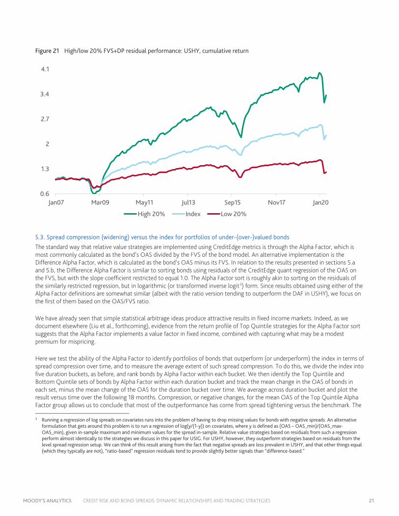
Finally, Figure 21 depicts the cumulative returns of the Top and Bottom Quintile Combined quant residual strategies using FVS and DP metrics, as well as the cumulative returns of the benchmark for comparison. The Top Quintile strategy outperforms the index considerably over time, and the Bottom Quintile strategy underperforms.
MOODY’S ANALYTICS CREDIT RISK AND BOND SPREADS: DYNAMIC RELATIONSHIPS AND TRADING STRATEGIES 21
Figure 21 High/low 20% FVS+DP residual performance: USHY, cumulative return
5.3. Spread compression (widening) versus the index for portfolios of under-(over-)valued bonds
The standard way that relative value strategies are implemented using CreditEdge metrics is through the Alpha Factor, which is most commonly calculated as the bond’s OAS divided by the FVS of the bond model. An alternative implementation is the Difference Alpha Factor, which is calculated as the bond’s OAS minus its FVS. In relation to the results presented in sections 5.a and 5.b, the Difference Alpha Factor is similar to sorting bonds using residuals of the CreditEdge quant regression of the OAS on the FVS, but with the slope coefficient restricted to equal 1.0. The Alpha Factor sort is roughly akin to sorting on the residuals of the similarly restricted regression, but in logarithmic (or transformed inverse logit3) form. Since results obtained using either of the Alpha Factor definitions are somewhat similar (albeit with the ratio version tending to outperform the DAF in USHY), we focus on the first of them based on the OAS/FVS ratio.
We have already seen that simple statistical arbitrage ideas produce attractive results in fixed income markets. Indeed, as we document elsewhere (Liu et al., forthcoming), evidence from the return profile of Top Quintile strategies for the Alpha Factor sort suggests that the Alpha Factor implements a value factor in fixed income, combined with capturing what may be a modest premium for mispricing.
Here we test the ability of the Alpha Factor to identify portfolios of bonds that outperform (or underperform) the index in terms of spread compression over time, and to measure the average extent of such spread compression. To do this, we divide the index into five duration buckets, as before, and rank bonds by Alpha Factor within each bucket. We then identify the Top Quintile and Bottom Quintile sets of bonds by Alpha Factor within each duration bucket and track the mean change in the OAS of bonds in each set, minus the mean change of the OAS for the duration bucket over time. We average across duration bucket and plot the result versus time over the following 18 months. Compression, or negative changes, for the mean OAS of the Top Quintile Alpha Factor group allows us to conclude that most of the outperformance has come from spread tightening versus the benchmark. The
3 Running a regression of log spreads on covariates runs into the problem of having to drop missing values for bonds with negative spreads. An alternative
formulation that gets around this problem is to run a regression of log(y/(1-y)) on covariates, where y is defined as (OAS – OAS_min)/(OAS_max-OAS_min), given in-sample maximum and minimum values for the spread in-sample. Relative value strategies based on residuals from such a regression perform almost identically to the strategies we discuss in this paper for USIG. For USHY, however, they outperform strategies based on residuals from the level spread regression setup. We can think of this result arising from the fact that negative spreads are less prevalent in USHY, and that other things equal (which they typically are not), “ratio-based” regression residuals tend to provide slightly better signals than “difference-based.”
0.6
1.3
2
2.7
3.4
4.1
Jan07 Mar09 May11 Jul13 Sep15 Nov17 Jan20
High 20% Index Low 20%
MOODY’S ANALYTICS CREDIT RISK AND BOND SPREADS: DYNAMIC RELATIONSHIPS AND TRADING STRATEGIES 22
same analysis can be done within DTS (duration times spread) bucket portfolios. DTS, as described Ben Dor et al. (2007), is regarded by many market participants as a more robust measure of risk in bond markets than the spread duration.
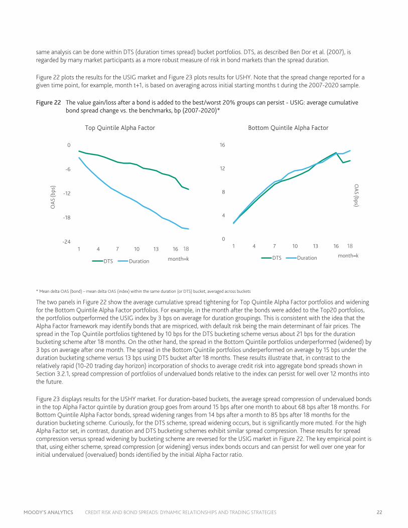
Figure 22 plots the results for the USIG market and Figure 23 plots results for USHY. Note that the spread change reported for a given time point, for example, month t+1, is based on averaging across initial starting months t during the 2007-2020 sample.
Figure 22 The value gain/loss after a bond is added to the best/worst 20% groups can persist - USIG: average cumulative bond spread change vs. the benchmarks, bp (2007-2020)*
Top Quintile Alpha Factor Bottom Quintile Alpha Factor
* Mean delta OAS (bond) – mean delta OAS (index) within the same duration (or DTS) bucket, averaged across buckets
The two panels in Figure 22 show the average cumulative spread tightening for Top Quintile Alpha Factor portfolios and widening for the Bottom Quintile Alpha Factor portfolios. For example, in the month after the bonds were added to the Top20 portfolios, the portfolios outperformed the USIG index by 3 bps on average for duration groupings. This is consistent with the idea that the Alpha Factor framework may identify bonds that are mispriced, with default risk being the main determinant of fair prices. The spread in the Top Quintile portfolios tightened by 10 bps for the DTS bucketing scheme versus about 21 bps for the duration bucketing scheme after 18 months. On the other hand, the spread in the Bottom Quintile portfolios underperformed (widened) by 3 bps on average after one month. The spread in the Bottom Quintile portfolios underperformed on average by 15 bps under the duration bucketing scheme versus 13 bps using DTS bucket after 18 months. These results illustrate that, in contrast to the relatively rapid (10-20 trading day horizon) incorporation of shocks to average credit risk into aggregate bond spreads shown in Section 3.2.1, spread compression of portfolios of undervalued bonds relative to the index can persist for well over 12 months into the future.
Figure 23 displays results for the USHY market. For duration-based buckets, the average spread compression of undervalued bonds in the top Alpha Factor quintile by duration group goes from around 15 bps after one month to about 68 bps after 18 months. For Bottom Quintile Alpha Factor bonds, spread widening ranges from 14 bps after a month to 85 bps after 18 months for the duration bucketing scheme. Curiously, for the DTS scheme, spread widening occurs, but is significantly more muted. For the high Alpha Factor set, in contrast, duration and DTS bucketing schemes exhibit similar spread compression. These results for spread compression versus spread widening by bucketing scheme are reversed for the USIG market in Figure 22. The key empirical point is that, using either scheme, spread compression (or widening) versus index bonds occurs and can persist for well over one year for initial undervalued (overvalued) bonds identified by the initial Alpha Factor ratio.
-24
-18
-12
-6
0
1 4 7 10 13 16
OAS
(bps
)
month=kDTS Duration
18
0
4
8
12
16
1 4 7 10 13 16
OAS (bps)
month=kDTS Duration
18

MOODY’S ANALYTICS CREDIT RISK AND BOND SPREADS: DYNAMIC RELATIONSHIPS AND TRADING STRATEGIES 23
Figure 23 The value gain/loss after a bond is added to the best/worst 20% groups can persist - USHY: average cumulative bond spread change vs. the benchmarks, bp (2007-2020)*
Top Quintile Alpha Factor Bottom Quintile Alpha Factor
* Mean delta OAS (bond) – mean delta OAS (index) within the same duration (or DTS) bucket, averaged across buckets
5.4. Sector-level convergence of model residuals to the mean
Having examined a class of strategies for exploiting reversion of bond spreads to fair values, as well as the extent of spread compression/widening relative to the index for a simple relative value strategy, we now turn to the sector dimension of the relative value phenomenon. Again, for simplicity we focus here on the Alpha Factor metric, which is defined as the ratio of the OAS of a bond to its FVS.
A sector-level version of the relative value convergence test is as follows: Do sectors with the highest and lowest mean OAS/FVS ratios see those ratios converge to the average, and if so, on what timescale does this occur?
To test this question, we use the 13 sector categories covered in the bond model that produces the FVS estimates. Using data from January 2007 to the end of April 2000, we computed the mean Alpha Factor, or OAS/FVS ratio, by sector each month. We then identified the sectors with the largest and smallest ratios each month and tracked the path of the mean sector OAS/FVS ratios for these sectors over the 20 months following the initial date. By averaging the results of this exercise over initial starting dates, we can form a picture of the mean convergence paths for the Max mean Alpha Factor and Min mean Alpha Factor sectors, respectively. The path for both Max and Min sectors for the USIG market is shown in Figure 24.
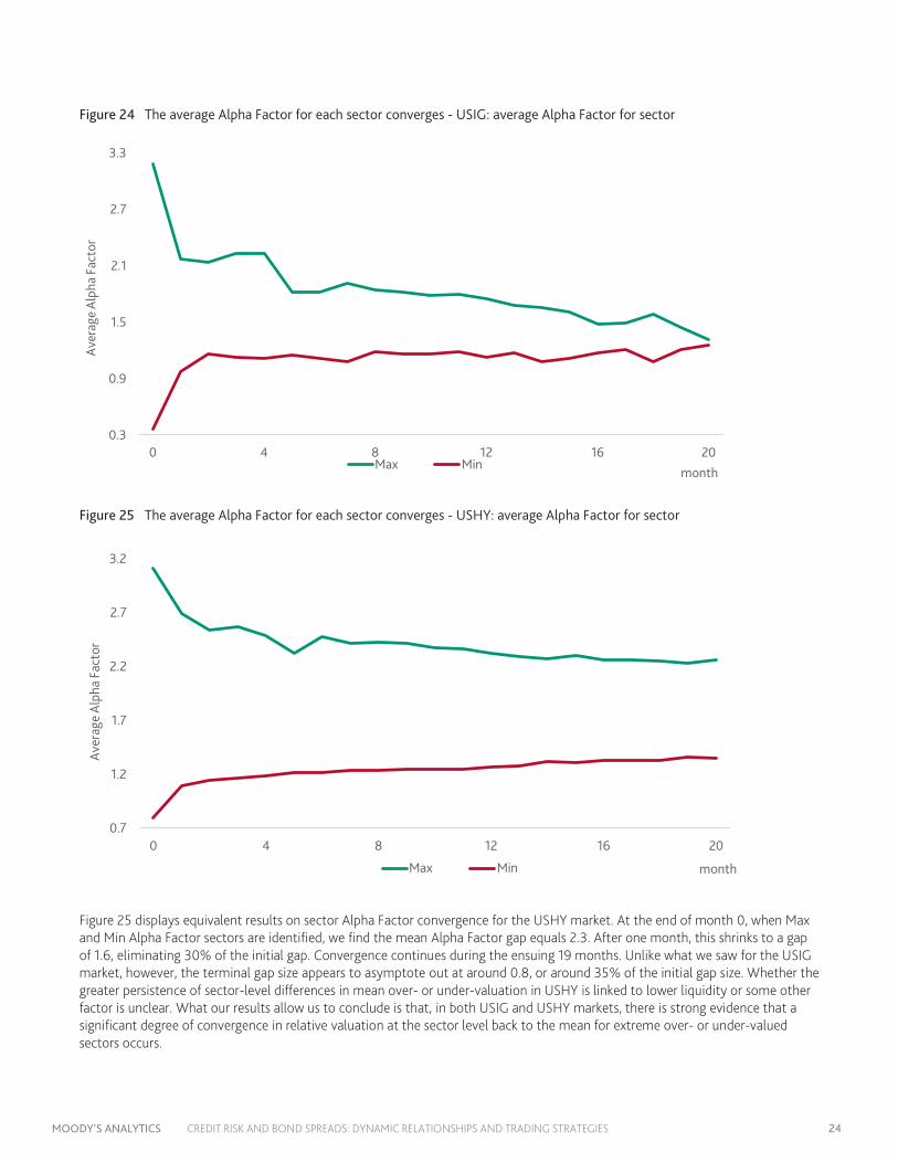
In the initial month, the average Alpha Factor for the sector with the Max Alpha Factor is 3.2 versus 0.3 for the Min Alpha Factor sector. By the first month, 59% of the initial gap of 2.9 between the mean Alpha Factor of the Max and Min sectors is eliminated, with the highest Alpha Factor sector converging somewhat faster. By month 20, the gap completely closes as the lines intersect. Thus, initial convergence is quick, but then the remaining 41% of the gap takes 19 additional months to disappear.
-85
-68
-51
-34
-17
0
1 4 7 10 13 16
OAS
(bps
)
month=kDTS Duration
18 0
17
34
51
68
85
1 4 7 10 13 16
OAS (bps)
month=kDTS Duration
18
MOODY’S ANALYTICS CREDIT RISK AND BOND SPREADS: DYNAMIC RELATIONSHIPS AND TRADING STRATEGIES 24
Figure 24 The average Alpha Factor for each sector converges - USIG: average Alpha Factor for sector
Figure 25 The average Alpha Factor for each sector converges - USHY: average Alpha Factor for sector
Figure 25 displays equivalent results on sector Alpha Factor convergence for the USHY market. At the end of month 0, when Max and Min Alpha Factor sectors are identified, we find the mean Alpha Factor gap equals 2.3. After one month, this shrinks to a gap of 1.6, eliminating 30% of the initial gap. Convergence continues during the ensuing 19 months. Unlike what we saw for the USIG market, however, the terminal gap size appears to asymptote out at around 0.8, or around 35% of the initial gap size. Whether the greater persistence of sector-level differences in mean over- or under-valuation in USHY is linked to lower liquidity or some other factor is unclear. What our results allow us to conclude is that, in both USIG and USHY markets, there is strong evidence that a significant degree of convergence in relative valuation at the sector level back to the mean for extreme over- or under-valued sectors occurs.
0.3
0.9
1.5
2.1
2.7
3.3
0 4 8 12 16 20
Aver
age
Alph
a Fa
ctor
monthMax Min
0.7
1.2
1.7
2.2
2.7
3.2
0 4 8 12 16 20
Aver
age
Alph
a Fa
ctor
monthMax Min

MOODY’S ANALYTICS CREDIT RISK AND BOND SPREADS: DYNAMIC RELATIONSHIPS AND TRADING STRATEGIES 25
6. Conclusion
In this article, we apply a range of tests to evaluate the existence and strength of different types of dynamic relationships between credit metrics and bond spreads. Despite doubts in the academic literature about the ability of structural credit risk models to explain the level of observed spreads, it is apparent that contemporaneous-level correlations between the mean default probability from a commercial structural credit risk model and mean bond spreads are quite high: 0.86 in USIG and 0.89 in USHY. Perhaps more importantly for institutional investors, there is robust evidence that credit risk metrics help predict time series movements of spreads as well as the cross-section of relative returns. In particular, default and downgrade probabilities have robust in-sample predictive power for spreads at the aggregate and individual bond levels. Bond spreads tend to rise considerably both prior to—and following—the breach by their issuers of high default and downgrade risk thresholds. Deviations of spreads from fair value implied by credit risk metrics help explain the cross section of next-month bond returns. The Sharpe ratios of high-minus-low residual strategies based on cross-sectional regressions improve upon those of the market benchmarks by 43% in both USIG and USHY. At the aggregate level, we observe the phenomenon that the mean ratio of market spreads to a measure of fair value spreads for the most under-valued and over-valued sectors tends to converge toward common levels over time. Collectively, the empirical regularities that we document in this paper are likely to have relevance for fixed-income traders, security selection, asset allocation, and the active management of bond portfolios.

MOODY’S ANALYTICS CREDIT RISK AND BOND SPREADS: DYNAMIC RELATIONSHIPS AND TRADING STRATEGIES 26
7. References
Almeida, Heitor and Philippon, Thomas (2007), “The risk-adjusted cost of financial distress”, The Journal of Finance, Vol. 62, Issue 6, pp. 2557-2586.
Bai, Jennie, Bali, Turan, and Wen, Quan (2019), “Common risk factors in the cross-section of corporate bond returns”, Journal of Financial Economics 131, pp. 619-642.
Bai, Jennie, Goldstein, Robert, and Yang, Fan, 2019, “Is the Credit Spread Puzzle a Myth?”, manuscript.
Ben Dor, Arik, Dynkin, Lev, Hyman, Jay, Houweling, Patrick, van Leeuwen, Erik, and Penninga, Olaf, DTSSM (Duration Times Spread) - A New Measure of Spread Exposure in Credit Portfolios, Lehman Brothers, The Journal of Portfolio Management Winter 2007, 33 (2) 77-100
Berndt, Antje, Douglas, Rohan, Duffie, Darrell, and Ferguson, Mark, 2018, “Corporate Credit Risk Premia”, Review of Finance, Volume 22, Issue 2, pp. 419-454.
Berndt, Antje, Ritchken, Peter, and Sun, Zhiqiang, 2009, “On correlation and default clustering in credit markets”, AFA 2010 Atlanta Meetings Paper. https://papers.ssrn.com/sol3/papers.cfm?abstract_id=1361328, Accessed on: August 6, 2020.
Bhamra, Harjoat, Kuehn, Lars-Alexander, and Strebulaev, Ilya, 2009, “The levered equity premium and credit spreads: A unified framework”, The Review of Financial Studies, Vol. 23, Issue 2, pp. 645-703.
Chen, Long, Collin-Dufresne, Pierre, and Goldstein, Robert, On the Relation Between Credit Spread Puzzle and the Equity Premium Puzzle. The Review of Financial Studies, Volume 22, Issue 9, September 2009.
Choi, Yukyung, Levine, Glenn, and Malone, Samuel (2020), “The coronavirus (COVID-19) pandemic: Assessing the impact on corporate credit risk”, Moody’s Analytics White Paper, https://www.moodysanalytics.com/articles/2020/coronavirus-assessing-the-impact-on-corporate-credit-risk, Accessed on: August 6, 2020.
Collin-Dufresne, Pierre, Goldstein, Robert, and Martin, Spencer (2001), “The Determinants of Credit Spread Changes”, Journal of Finance, 56, 2177-2207
Dwyer, Douglas, Li, Zan, Qu, Shisheng, Russell, Heather, and Zhang, Jing, “ CDS-implied EDF Credit Measures and Fair-value Spreads”, Moody’s Analytics White Paper, March 2010.
Feldhütter, Peter, and Schaefer, Stephen, 2018. The myth of the credit spread puzzle. Review of Financial Studies 31, 351-367.
Granger, C. W. J. (1969). "Investigating Causal Relations by Econometric Models and Cross-spectral Methods". Econometrica. 37 (3): 424–438. doi:10.2307/1912791.
Grinold, Richard and Kahn, Ronald, 2020, “Advances in Active Portfolio Management”, McGraw Hill, New York.
Huang, Jing-Zhi and Huang, Ming, 2003, “How Much of the Corporate-Treasury Yield Spread is Due to Credit Risk?”, 2003 Western Finance Association Meetings.
Huang, Jing-Zhi, Nozawa, Yohio, and Shi, Zhan, 2019, “The Global Credit Spread Puzzle”, Available at SSRN: https://ssrn.com/abstract=3453959 or http://dx.doi.org/10.2139/ssrn.3453959
Israel, Ronen, Palhares, Diogo, and Richardson, Scott, Common Factors in Corporate Bond Returns, Journal of Investment Management, 2018, Vol. 16, No.2

MOODY’S ANALYTICS CREDIT RISK AND BOND SPREADS: DYNAMIC RELATIONSHIPS AND TRADING STRATEGIES 27
Krishnan, C.N., Ritchken, Peter, and Thomson, James, Predicting Credit Spreads, 2010, Journal of Financial Intermediation, Vol. 19, Issue 4, pp. 529-563.
Luetkepohl, Helmut, 2017, “Estimation of structural vector autoregressive models”, Communications for Statistical Applications and Methods, Vol. 24, pp. 421-441.
Li, Zan, Zhang, Jing, and Crossen, Christopher, 2012, “A Model-Based Approach to Constructing Corporate Bond Portfolios”, The Journal of Fixed Income, Vol. 22, No. 2.
Liu, Peter, Zhuang, Zhong, Dwyer, Douglas, Choi, Yukyung, and Malone, Samuel, “ Moody’s Analytics EDF-Based Bond Valuation Model v2.0”, forthcoming.
Malone, Samuel, Baron, Irina, and White, Reginald, “The Deterioration Probability (DP) Model : Methodology and Validation”, Moody’s Analytics White Paper, March 2018.
Nazeran, Pooya and Dwyer, Douglas, 2015, “Credit Risk Modeling of Public Firms: EDF9”, Moody’s Analytics White Paper.
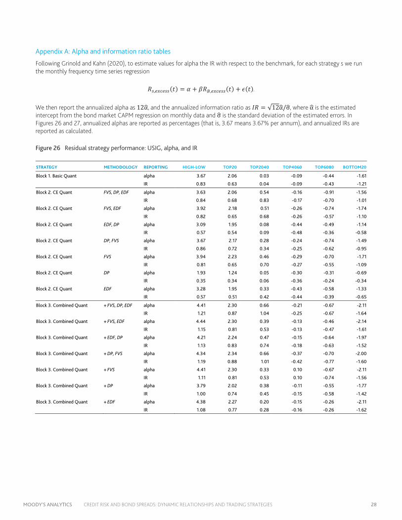
MOODY’S ANALYTICS CREDIT RISK AND BOND SPREADS: DYNAMIC RELATIONSHIPS AND TRADING STRATEGIES 28
Appendix A: Alpha and information ratio tables
Following Grinold and Kahn (2020), to estimate values for alpha the IR with respect to the benchmark, for each strategy s we run the monthly frequency time series regression
𝑀𝑀𝐵𝐵,𝑒𝑒𝑒𝑒𝐵𝐵𝑒𝑒𝐵𝐵𝐵𝐵(𝐷𝐷) = 𝛼𝛼 + 𝛽𝛽𝑀𝑀𝐵𝐵,𝑒𝑒𝑒𝑒𝐵𝐵𝑒𝑒𝐵𝐵𝐵𝐵(𝐷𝐷) + 𝜖𝜖(𝐷𝐷).
We then report the annualized alpha as 12α�, and the annualized information ratio as 𝐼𝐼𝑀𝑀 = √12α�/σ�, where α� is the estimated intercept from the bond market CAPM regression on monthly data and σ� is the standard deviation of the estimated errors. In Figures 26 and 27, annualized alphas are reported as percentages (that is, 3.67 means 3.67% per annum), and annualized IRs are reported as calculated.
Figure 26 Residual strategy performance: USIG, alpha, and IR
STRATEGY METHODOLOGY REPORTING HIGH-LOW TOP20 TOP2040 TOP4060 TOP6080 BOTTOM20
Block 1. Basic Quant alpha 3.67 2.06 0.03 -0.09 -0.44 -1.61 IR 0.83 0.63 0.04 -0.09 -0.43 -1.21
Block 2. CE Quant FVS, DP, EDF alpha 3.63 2.06 0.54 -0.16 -0.91 -1.56 IR 0.84 0.68 0.83 -0.17 -0.70 -1.01
Block 2. CE Quant FVS, EDF alpha 3.92 2.18 0.51 -0.26 -0.74 -1.74 IR 0.82 0.65 0.68 -0.26 -0.57 -1.10
Block 2. CE Quant EDF, DP alpha 3.09 1.95 0.08 -0.44 -0.49 -1.14 IR 0.57 0.54 0.09 -0.48 -0.36 -0.58
Block 2. CE Quant DP, FVS alpha 3.67 2.17 0.28 -0.24 -0.74 -1.49 IR 0.86 0.72 0.34 -0.25 -0.62 -0.95
Block 2. CE Quant FVS alpha 3.94 2.23 0.46 -0.29 -0.70 -1.71 IR 0.81 0.65 0.70 -0.27 -0.55 -1.09
Block 2. CE Quant DP alpha 1.93 1.24 0.05 -0.30 -0.31 -0.69 IR 0.35 0.34 0.06 -0.36 -0.24 -0.34
Block 2. CE Quant EDF alpha 3.28 1.95 0.33 -0.43 -0.58 -1.33 IR 0.57 0.51 0.42 -0.44 -0.39 -0.65
Block 3. Combined Quant + FVS, DP, EDF alpha 4.41 2.30 0.66 -0.21 -0.67 -2.11 IR 1.21 0.87 1.04 -0.25 -0.67 -1.64
Block 3. Combined Quant + FVS, EDF alpha 4.44 2.30 0.39 -0.13 -0.46 -2.14 IR 1.15 0.81 0.53 -0.13 -0.47 -1.61
Block 3. Combined Quant + EDF, DP alpha 4.21 2.24 0.47 -0.15 -0.64 -1.97 IR 1.13 0.83 0.74 -0.18 -0.63 -1.52
Block 3. Combined Quant + DP, FVS alpha 4.34 2.34 0.66 -0.37 -0.70 -2.00 IR 1.19 0.88 1.01 -0.42 -0.77 -1.60
Block 3. Combined Quant + FVS alpha 4.41 2.30 0.33 0.10 -0.67 -2.11 IR 1.11 0.81 0.53 0.10 -0.74 -1.56
Block 3. Combined Quant + DP alpha 3.79 2.02 0.38 -0.11 -0.55 -1.77 IR 1.00 0.74 0.45 -0.15 -0.58 -1.42
Block 3. Combined Quant + EDF alpha 4.38 2.27 0.20 -0.15 -0.26 -2.11 IR 1.08 0.77 0.28 -0.16 -0.26 -1.62
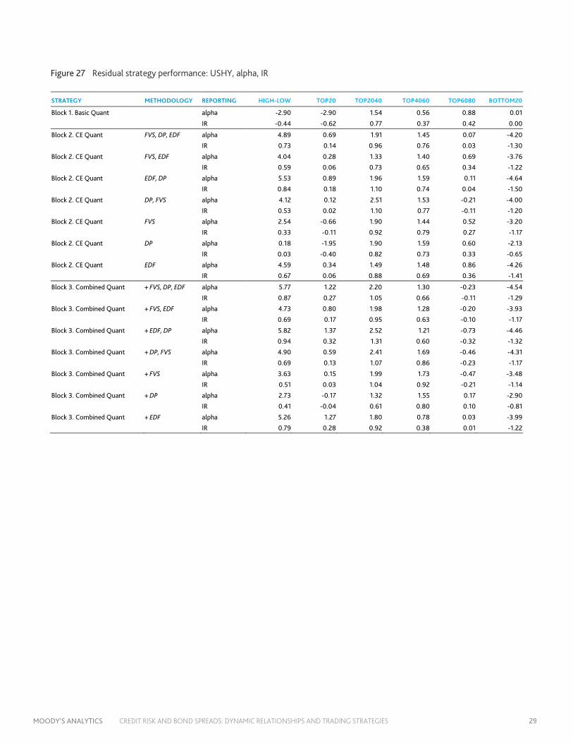
MOODY’S ANALYTICS CREDIT RISK AND BOND SPREADS: DYNAMIC RELATIONSHIPS AND TRADING STRATEGIES 29
Figure 27 Residual strategy performance: USHY, alpha, IR
STRATEGY METHODOLOGY REPORTING HIGH-LOW TOP20 TOP2040 TOP4060 TOP6080 BOTTOM20
Block 1. Basic Quant alpha -2.90 -2.90 1.54 0.56 0.88 0.01 IR -0.44 -0.62 0.77 0.37 0.42 0.00
Block 2. CE Quant FVS, DP, EDF alpha 4.89 0.69 1.91 1.45 0.07 -4.20 IR 0.73 0.14 0.96 0.76 0.03 -1.30
Block 2. CE Quant FVS, EDF alpha 4.04 0.28 1.33 1.40 0.69 -3.76 IR 0.59 0.06 0.73 0.65 0.34 -1.22
Block 2. CE Quant EDF, DP alpha 5.53 0.89 1.96 1.59 0.11 -4.64 IR 0.84 0.18 1.10 0.74 0.04 -1.50
Block 2. CE Quant DP, FVS alpha 4.12 0.12 2.51 1.53 -0.21 -4.00 IR 0.53 0.02 1.10 0.77 -0.11 -1.20
Block 2. CE Quant FVS alpha 2.54 -0.66 1.90 1.44 0.52 -3.20 IR 0.33 -0.11 0.92 0.79 0.27 -1.17
Block 2. CE Quant DP alpha 0.18 -1.95 1.90 1.59 0.60 -2.13 IR 0.03 -0.40 0.82 0.73 0.33 -0.65
Block 2. CE Quant EDF alpha 4.59 0.34 1.49 1.48 0.86 -4.26 IR 0.67 0.06 0.88 0.69 0.36 -1.41
Block 3. Combined Quant + FVS, DP, EDF alpha 5.77 1.22 2.20 1.30 -0.23 -4.54 IR 0.87 0.27 1.05 0.66 -0.11 -1.29
Block 3. Combined Quant + FVS, EDF alpha 4.73 0.80 1.98 1.28 -0.20 -3.93 IR 0.69 0.17 0.95 0.63 -0.10 -1.17
Block 3. Combined Quant + EDF, DP alpha 5.82 1.37 2.52 1.21 -0.73 -4.46 IR 0.94 0.32 1.31 0.60 -0.32 -1.32
Block 3. Combined Quant + DP, FVS alpha 4.90 0.59 2.41 1.69 -0.46 -4.31 IR 0.69 0.13 1.07 0.86 -0.23 -1.17
Block 3. Combined Quant + FVS alpha 3.63 0.15 1.99 1.73 -0.47 -3.48 IR 0.51 0.03 1.04 0.92 -0.21 -1.14
Block 3. Combined Quant + DP alpha 2.73 -0.17 1.32 1.55 0.17 -2.90 IR 0.41 -0.04 0.61 0.80 0.10 -0.81
Block 3. Combined Quant + EDF alpha 5.26 1.27 1.80 0.78 0.03 -3.99 IR 0.79 0.28 0.92 0.38 0.01 -1.22

MOODY’S ANALYTICS CREDIT RISK AND BOND SPREADS: DYNAMIC RELATIONSHIPS AND TRADING STRATEGIES BX1456
© 2020 Moody’s Corporation, Moody’s Investors Service, Inc., Moody’s Analytics, Inc. and/or their licensors and affiliates (collectively, “MOODY’S”). All rights reserved.
CREDIT RATINGS ISSUED BY MOODY'S INVESTORS SERVICE, INC. AND/OR ITS CREDIT RATINGS AFFILIATES ARE MOODY’S CURRENT OPINIONS OF THE RELATIVE FUTURE CREDIT RISK OF ENTITIES, CREDIT COMMITMENTS, OR DEBT OR DEBT-LIKE SECURITIES, AND MATERIALS, PRODUCTS, SERVICES AND INFORMATION PUBLISHED BY MOODY’S (COLLECTIVELY, “PUBLICATIONS”) MAY INCLUDE SUCH CURRENT OPINIONS. MOODY’S INVESTORS SERVICE DEFINES CREDIT RISK AS THE RISK THAT AN ENTITY MAY NOT MEET ITS CONTRACTUAL FINANCIAL OBLIGATIONS AS THEY COME DUE AND ANY ESTIMATED FINANCIAL LOSS IN THE EVENT OF DEFAULT OR IMPAIRMENT. SEE MOODY’S RATING SYMBOLS AND DEFINITIONS PUBLICATION FOR INFORMATION ON THE TYPES OF CONTRACTUAL FINANCIAL OBLIGATIONS ADDRESSED BY MOODY’S INVESTORS SERVICE CREDIT RATINGS. CREDIT RATINGS DO NOT ADDRESS ANY OTHER RISK, INCLUDING BUT NOT LIMITED TO: LIQUIDITY RISK, MARKET VALUE RISK, OR PRICE VOLATILITY. CREDIT RATINGS, NON-CREDIT ASSESSMENTS (“ASSESSMENTS”), AND OTHER OPINIONS INCLUDED IN MOODY’S PUBLICATIONS ARE NOT STATEMENTS OF CURRENT OR HISTORICAL FACT. MOODY’S PUBLICATIONS MAY ALSO INCLUDE QUANTITATIVE MODEL-BASED ESTIMATES OF CREDIT RISK AND RELATED OPINIONS OR COMMENTARY PUBLISHED BY MOODY’S ANALYTICS, INC. AND/OR ITS AFFILIATES. MOODY’S CREDIT RATINGS, ASSESSMENTS, OTHER OPINIONS AND PUBLICATIONS DO NOT CONSTITUTE OR PROVIDE INVESTMENT OR FINANCIAL ADVICE, AND MOODY’S CREDIT RATINGS, ASSESSMENTS, OTHER OPINIONS AND PUBLICATIONS ARE NOT AND DO NOT PROVIDE RECOMMENDATIONS TO PURCHASE, SELL, OR HOLD PARTICULAR SECURITIES. MOODY’S CREDIT RATINGS, ASSESSMENTS, OTHER OPINIONS AND PUBLICATIONS DO NOT COMMENT ON THE SUITABILITY OF AN INVESTMENT FOR ANY PARTICULAR INVESTOR. MOODY’S ISSUES ITS CREDIT RATINGS, ASSESSMENTS AND OTHER OPINIONS AND PUBLISHES ITS PUBLICATIONS WITH THE EXPECTATION AND UNDERSTANDING THAT EACH INVESTOR WILL, WITH DUE CARE, MAKE ITS OWN STUDY AND EVALUATION OF EACH SECURITY THAT IS UNDER CONSIDERATION FOR PURCHASE, HOLDING, OR SALE.
MOODY’S CREDIT RATINGS, ASSESSMENTS, OTHER OPINIONS, AND PUBLICATIONS ARE NOT INTENDED FOR USE BY RETAIL INVESTORS AND IT WOULD BE RECKLESS AND INAPPROPRIATE FOR RETAIL INVESTORS TO USE MOODY’S CREDIT RATINGS, ASSESSMENTS, OTHER OPINIONS OR PUBLICATIONS WHEN MAKING AN INVESTMENT DECISION. IF IN DOUBT YOU SHOULD CONTACT YOUR FINANCIAL OR OTHER PROFESSIONAL ADVISER.
ALL INFORMATION CONTAINED HEREIN IS PROTECTED BY LAW, INCLUDING BUT NOT LIMITED TO, COPYRIGHT LAW, AND NONE OF SUCH INFORMATION MAY BE COPIED OR OTHERWISE REPRODUCED, REPACKAGED, FURTHER TRANSMITTED, TRANSFERRED, DISSEMINATED, REDISTRIBUTED OR RESOLD, OR STORED FOR SUBSEQUENT USE FOR ANY SUCH PURPOSE, IN WHOLE OR IN PART, IN ANY FORM OR MANNER OR BY ANY MEANS WHATSOEVER, BY ANY PERSON WITHOUT MOODY’S PRIOR WRITTEN CONSENT.
MOODY’S CREDIT RATINGS, ASSESSMENTS, OTHER OPINIONS AND PUBLICATIONS ARE NOT INTENDED FOR USE BY ANY PERSON AS A BENCHMARK AS THAT TERM IS DEFINED FOR REGULATORY PURPOSES AND MUST NOT BE USED IN ANY WAY THAT COULD RESULT IN THEM BEING CONSIDERED A BENCHMARK.
All information contained herein is obtained by MOODY’S from sources believed by it to be accurate and reliable. Because of the possibility of human or mechanical error as well as other factors, however, all information contained herein is provided “AS IS” without warranty of any kind. MOODY'S adopts all necessary measures so that the information it uses in assigning a credit rating is of sufficient quality and from sources MOODY'S considers to be reliable including, when appropriate, independent third-party sources. However, MOODY’S is not an auditor and cannot in every instance independently verify or validate information received in the rating process or in preparing its Publications.
To the extent permitted by law, MOODY’S and its directors, officers, employees, agents, representatives, licensors and suppliers disclaim liability to any person or entity for any indirect, special, consequential, or incidental losses or damages whatsoever arising from or in connection with the information contained herein or the use of or inability to use any such information, even if MOODY’S or any of its directors, officers, employees, agents, representatives, licensors or suppliers is advised in advance of the possibility of such losses or damages, including but not limited to: (a) any loss of present or prospective profits or (b) any loss or damage arising where the relevant financial instrument is not the subject of a particular credit rating assigned by MOODY’S.
To the extent permitted by law, MOODY’S and its directors, officers, employees, agents, representatives, licensors and suppliers disclaim liability for any direct or compensatory losses or damages caused to any person or entity, including but not limited to by any negligence (but excluding fraud, willful misconduct or any other type of liability that, for the avoidance of doubt, by law cannot be excluded) on the part of, or any contingency within or beyond the control of, MOODY’S or any of its directors, officers, employees, agents, representatives, licensors or suppliers, arising from or in connection with the information contained herein or the use of or inability to use any such information.
NO WARRANTY, EXPRESS OR IMPLIED, AS TO THE ACCURACY, TIMELINESS, COMPLETENESS, MERCHANTABILITY OR FITNESS FOR ANY PARTICULAR PURPOSE OF ANY CREDIT RATING, ASSESSMENT, OTHER OPINION OR INFORMATION IS GIVEN OR MADE BY MOODY’S IN ANY FORM OR MANNER WHATSOEVER.
Moody’s Investors Service, Inc., a wholly-owned credit rating agency subsidiary of Moody’s Corporation (“MCO”), hereby discloses that most issuers of debt securities (including corporate and municipal bonds, debentures, notes and commercial paper) and preferred stock rated by Moody’s Investors Service, Inc. have, prior to assignment of any credit rating, agreed to pay to Moody’s Investors Service, Inc. for credit ratings opinions and services rendered by it fees ranging from $1,000 to approximately $2,700,000. MCO and Moody’s investors Service also maintain policies and procedures to address the independence of Moody’s Investors Service credit ratings and credit rating processes. Information regarding certain affiliations that may exist between directors of MCO and rated entities, and between entities who hold credit ratings from Moody’s Investors Service and have also publicly reported to the SEC an ownership interest in MCO of more than 5%, is posted annually at www.moodys.com under the heading “Investor Relations — Corporate Governance — Director and Shareholder Affiliation Policy.”
Additional terms for Australia only: Any publication into Australia of this document is pursuant to the Australian Financial Services License of MOODY’S affiliate, Moody’s Investors Service Pty Limited ABN 61 003 399 657AFSL 336969 and/or Moody’s Analytics Australia Pty Ltd ABN 94 105 136 972 AFSL 383569 (as applicable). This document is intended to be provided only to “wholesale clients” within the meaning of section 761G of the Corporations Act 2001. By continuing to access this document from within Australia, you represent to MOODY’S that you are, or are accessing the document as a representative of, a “wholesale client” and that neither you nor the entity you represent will directly or indirectly disseminate this document or its contents to “retail clients” within the meaning of section 761G of the Corporations Act 2001. MOODY’S credit rating is an opinion as to the creditworthiness of a debt obligation of the issuer, not on the equity securities of the issuer or any form of security that is available to retail investors.
Additional terms for Japan only: Moody's Japan K.K. (“MJKK”) is a wholly-owned credit rating agency subsidiary of Moody's Group Japan G.K., which is wholly-owned by Moody’s Overseas Holdings Inc., a wholly-owned subsidiary of MCO. Moody’s SF Japan K.K. (“MSFJ”) is a wholly-owned credit rating agency subsidiary of MJKK. MSFJ is not a Nationally Recognized Statistical Rating Organization (“NRSRO”). Therefore, credit ratings assigned by MSFJ are Non-NRSRO Credit Ratings. Non-NRSRO Credit Ratings are assigned by an entity that is not a NRSRO and, consequently, the rated obligation will not qualify for certain types of treatment under U.S. laws. MJKK and MSFJ are credit rating agencies registered with the Japan Financial Services Agency and their registration numbers are FSA Commissioner (Ratings) No. 2 and 3 respectively.
MJKK or MSFJ (as applicable) hereby disclose that most issuers of debt securities (including corporate and municipal bonds, debentures, notes and commercial paper) and preferred stock rated by MJKK or MSFJ (as applicable) have, prior to assignment of any credit rating, agreed to pay to MJKK or MSFJ (as applicable) for credit ratings opinions and services rendered by it fees ranging from JPY125,000 to approximately JPY250,000,000.
MJKK and MSFJ also maintain policies and procedures to address Japanese regulatory requirements.