Real-Time Volumetric Lighting using SVOs

Victor Strömberg

MASTER’S THESIS | LUND UNIVERSITY 2015

Department of Computer ScienceFaculty of Engineering LTH

ISSN 1650-2884 LU-CS-EX 2015-39

Real-Time Volumetric Lighting usingSVOs

Victor Strömbergada10vru@student.lu.se

September 17, 2015

Master's thesis work carried out atthe Department of Computer Science, Lund University.

Supervisor: Michael Doggett, michael.doggett@cs.lth.se

Examiner: Flavius Gruian, Flavius.Gruian@cs.lth.se

Abstract

This thesis experiments with the data structure of a sparse voxel octree (SVO)to see if it may improve the performance of empty space ray marching in vol-umes. While ray marching is a somewhat new technique it is used more of-ten in traversal of volumes. It can be used for realistic volumetric effects incomputer games or it can be used in the medical field when examining andvisualizing MRI scans. While it has many uses it is however very computa-tionally heavy. The usage in real-time applications is therefore limited as thehardware must be able to maintain enough frames per second to satisfy thestandard. Normally one would sample the volume with a fixed sample step inorder to extract the information in the volume, even if there is just empty space.The idea of a sparse octree is that it allows the ray to take greater steps pastthis empty space and thus only sample the actual data. This thesis will explainhow to implement and use an octree when rendering smoke in a volume, andshowcasing the many challenges that comes with this. The result is comparedwith a three dimensional texture of the same smoke.

Keywords: Sparse voxel octree, ray marching, volume, real-time, 3D texture

2

Acknowledgements

I would like to thank my supervisor Ass. Prof. Michael Doggett for all the helpful discus-sions and guidance regarding this thesis. I would also like to thank Per Ganestam for inputand help regarding general GPU and GLSL questions.

3

4

Contents

1 Introduction 71.1 Background . . . . . . . . . . . . . . . . . . . . . . . . . . . . . . . . . 8

1.1.1 OpenGL . . . . . . . . . . . . . . . . . . . . . . . . . . . . . . . 81.1.2 Compute Shaders . . . . . . . . . . . . . . . . . . . . . . . . . . 81.1.3 Ray marching . . . . . . . . . . . . . . . . . . . . . . . . . . . . 111.1.4 Octree . . . . . . . . . . . . . . . . . . . . . . . . . . . . . . . . 131.1.5 Voxels . . . . . . . . . . . . . . . . . . . . . . . . . . . . . . . . 141.1.6 Noise . . . . . . . . . . . . . . . . . . . . . . . . . . . . . . . . 15

1.2 Related work . . . . . . . . . . . . . . . . . . . . . . . . . . . . . . . . 151.3 Problem and contribution . . . . . . . . . . . . . . . . . . . . . . . . . . 161.4 Report structure . . . . . . . . . . . . . . . . . . . . . . . . . . . . . . . 16

2 Implementation 192.1 Full screen quad . . . . . . . . . . . . . . . . . . . . . . . . . . . . . . . 192.2 Noise . . . . . . . . . . . . . . . . . . . . . . . . . . . . . . . . . . . . 202.3 Constructing the octree . . . . . . . . . . . . . . . . . . . . . . . . . . . 21

2.3.1 The octree array . . . . . . . . . . . . . . . . . . . . . . . . . . 232.4 Ray marching . . . . . . . . . . . . . . . . . . . . . . . . . . . . . . . . 25

2.4.1 Traversing the octree . . . . . . . . . . . . . . . . . . . . . . . . 27

3 Results 313.1 Measurements . . . . . . . . . . . . . . . . . . . . . . . . . . . . . . . . 313.2 Visual comparison . . . . . . . . . . . . . . . . . . . . . . . . . . . . . 32

4 Discussion 41

5 Conclusion 45

Bibliography 47

5

CONTENTS

6

Chapter 1Introduction

Many phenomena in the real world are hard to approximate and represent using geometricsurfaces. This includes, but is not limited to, clouds, smoke, fire and explosions. The ap-pearance of these effects is caused by the cumulative light emitted, scattered and absorbedby a huge number of particles. These effects are usually approximated today with particlesystems, but as these are hard to get accurate effects of without using a lot of memory andcomputational power, they have their limits in real-time games. Another way of simulatingthis is the use of volumes.

Volume rendering is represented as a uniform three dimensional array of samples,which can be pre-computed or procedurally generated. The final image is created by sam-pling this volume by taking steps along the viewing rays and accumulating data throughoutthe volume. Often these volumes are represented with simple geometry such as a cube ora sphere, making it easy to check for enter and exit boundaries. However, using volumerendering is not cheap and is something that is hard to integrate with real-time standards.One issue is that if the volume contains a lot of empty spaces one would risk the computa-tional power of sampling nothing, when it is the actual data one is interested in. To tacklethis issue we introduce a sparse voxel octree as an alternative data representation of thevolume, then traverse this octree in real-time on the GPU.

7

1. I

1.1 Background1.1.1 OpenGLOpenGL is an API for interacting with a graphics card. It provides a rendering pipeline thatthe graphics card can use to output images on the computer. The programming languageGLSL is its high level shading language that enables programming of shaders in a C-stylesyntax. The main idea was to give programmers more direct control over the pipelinewithout having to use assembly language or hardware-specific languages.

The current version of GLSL is 4.5. With version 4.3 the Shader Storage Buffer Object(SSBO) was introduced [7], making it possible to allocate memory on the GPU and todynamically read and write to this. Normal buffers like a Uniform Buffer Object has a sizelimit of at least 16KB. An SSBO has at least 16MB, but usually more depending on theavailable GPU memory at hand. This is important for this project as we need to send inlarge amounts of data for our tree.

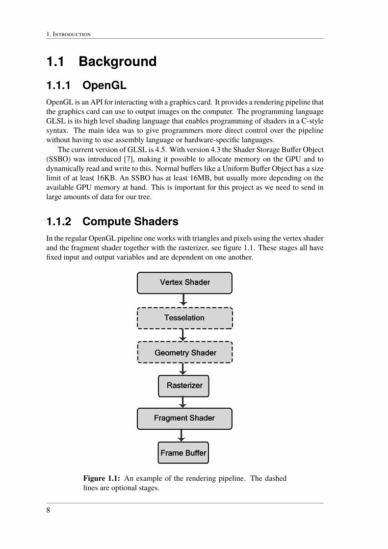
1.1.2 Compute ShadersIn the regular OpenGL pipeline one works with triangles and pixels using the vertex shaderand the fragment shader together with the rasterizer, see figure 1.1. These stages all havefixed input and output variables and are dependent on one another.

Figure 1.1: An example of the rendering pipeline. The dashedlines are optional stages.

8

1.1 B

A compute shader is a separate shader stage not used in the rendering pipeline. It issolely used for computing arbitrary information using the GPU's great parallelism. Thecompute shader does not have any defined input or output variables. It is up to the user tofetch and set these depending on the purpose of the shader. If a compute shader wants totake some value as input then it would have to fetch these as texture access, shader storageblocks, uniforms, images or other forms of interfaces. Likewise, to output something itmust explicitly write to a shader storage block or an image.

How often a shader executes depends on what kind of shader it is. For example, vertexshaders execute once per input vertex and the fragment shaders execute on fragments gen-erated by the rasterization stage. A compute shader does not have any pre-defined ''space''it executes in, it is up to each shader to define. To define this we introduce the abstractconcept of work groups.

A work group is the smallest amount of compute operations a user can execute. Anynumber of work groups may be executed and they are defined when invoking the computeoperation, see figure 1.2. The space these groups work in is three dimensional, i.e. ithas a number of X,Y and Z groups. Any of these may be set to 1, enabling a one, two orthree dimensional compute depending on the application. However this merely determineshow the coordinates are provided to the shader. In the end what counts is the number ofinvocations in the work group, that is the product of these three numbers.

Figure 1.2: Illustration of work groups in a compute dispatch.

When computing these work groups the system can do so in any order. For example, fora given work group of (3,2,1) it could execute group (0,0,1) first, followed by (3,0,0), thenjump to (2,1,2). This means that the compute shader should not rely on the order in whichindividual groups are processed. A single work group is not the same as a single computeshader invocation. Within a work group there may be many compute shader invocations.How many is defined by the compute shader itself and not by the call that executes it. Thisis the local size of the work group. If the local size is (128,1,1) and the group count is(16,8,64), this will give 1,048,576 separate shader invocations, each having a set of inputs

9

1. I

that uniquely identifies that invocation.

Figure 1.3: Illustration of the inside of a work group.

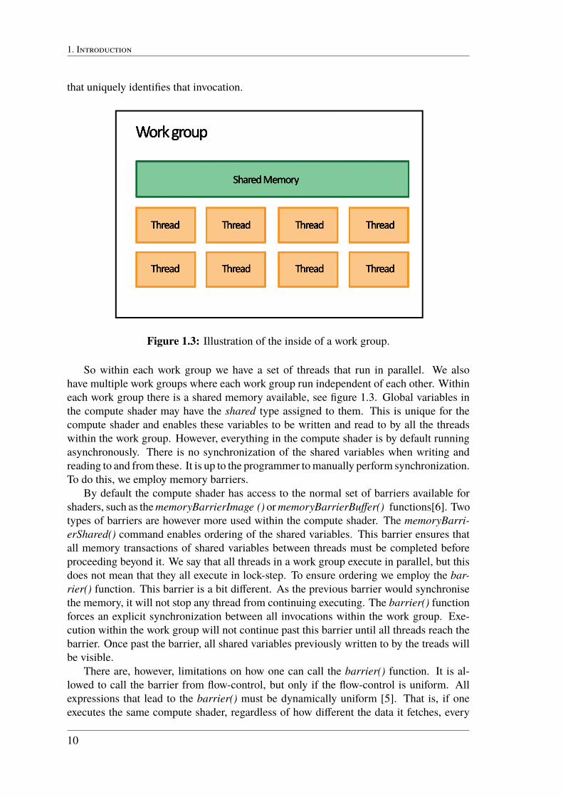
So within each work group we have a set of threads that run in parallel. We alsohave multiple work groups where each work group run independent of each other. Withineach work group there is a shared memory available, see figure 1.3. Global variables inthe compute shader may have the shared type assigned to them. This is unique for thecompute shader and enables these variables to be written and read to by all the threadswithin the work group. However, everything in the compute shader is by default runningasynchronously. There is no synchronization of the shared variables when writing andreading to and from these. It is up to the programmer to manually perform synchronization.To do this, we employ memory barriers.

By default the compute shader has access to the normal set of barriers available forshaders, such as the memoryBarrierImage�() or memoryBarrierBuffer()� functions[6]. Twotypes of barriers are however more used within the compute shader. The memoryBarri-erShared() command enables ordering of the shared variables. This barrier ensures thatall memory transactions of shared variables between threads must be completed beforeproceeding beyond it. We say that all threads in a work group execute in parallel, but thisdoes not mean that they all execute in lock-step. To ensure ordering we employ the bar-rier() function. This barrier is a bit different. As the previous barrier would synchronisethe memory, it will not stop any thread from continuing executing. The barrier() functionforces an explicit synchronization between all invocations within the work group. Exe-cution within the work group will not continue past this barrier until all threads reach thebarrier. Once past the barrier, all shared variables previously written to by the treads willbe visible.

There are, however, limitations on how one can call the barrier() function. It is al-lowed to call the barrier from flow-control, but only if the flow-control is uniform. Allexpressions that lead to the barrier() must be dynamically uniform [5]. That is, if oneexecutes the same compute shader, regardless of how different the data it fetches, every

10

1.1 B

single execution must hit the exact same set of barrier() in the exact same order. If not,unpredicted synchronization errors may occur [4]. Consider the code snippet below. Theuniform variable is a variable that is constant and can not change during execution.

if(uniform > 1.0){barrier();

}

This is ok since this condition can be evaluated at runtime, it will not change, and willpass or fail for every thread.

if(someVariable > 1.0){barrier();

}

May fail depending on whether someVariable changes during execution. It can not beguaranteed that each thread take this branch in the exact same way.

1.1.3 Ray marchingRay marching is a three dimensional rendering technique that is often used with volumesand visualizing three dimensional data structures. Imagine an object in a space but youdo not have any formula or triangles to describe it. The only thing you can find out is thedistance to this object from any given point.

Figure 1.4: Illustration of the concept of ray casting. The bluesquare symbolizes a pixel on the plane. The yellow figure repre-sents an object in our scene. For each pixel on the plane we shoota ray and see what we hit.

11

1. I

The basic idea is simple. Imagine that your eye is the camera and the monitor you arelooking at is the surface in some space, the image plane. For each pixel on this plane shoota ray from you eye into the pixel and through. Find the closest object blocking the pathof the ray and if it hits we can compute the color, shading or other attributes dependingon the application. If it does not hit we may color it with some sky color or simply black.This is called ray casting, see figure 1.4.

There are different ways of calculating the intersection of an object. A ray tracer usesan analytical algorithm to solve for it. A ray marcher, however, uses a more approximateapproach. By marching along the ray in steps, and for each step check how close weare to an object, we can create an approximate surface of this object and call it a hit.However, by taking too small steps the computation cost becomes too great and will effectthe performance negatively. Likewise, taking too large steps will jeopardize the accuracyand may result in stepping over the object in question. To solve this we use distance fields.

Distance fieldsUsing distance fields we can enable a variable step size. By measuring the shortest distanceto each object's surface in the scene for every step we take along the ray, we can make sureto only step forward that much without risking overshooting, see figure 1.5. To measurethe distance to objects we use distance estimators.

Eye

Figure 1.5: Illustration of variable step size using distance fields.The black dots represent the steps taken. The orange circles indi-cate the distance to the closest object, enabling a safe step lengthfor that point. When we have reached a threshold of how close weshould be, we say we hit the surface.

Distance estimators are compact functions that describe a geometric object in three

12

1.1 B

dimensional space. The object could for example be a sphere, a box or a triangle. Afunction that gives a sphere with radius r at the origin in our scene would be:

float distSphere(vec3 p, float r) {return length(p) - r;

}

and a function for a box with position b is [13]:

float unsignedBox(vec3 p, vec3 b){return length(max(abs(p)-b,0.0));

}

These functions calculate the distance between a point p and itself. The functions canbe signed or unsigned. A signed function returns the signed distance to this object. If weare inside the object we would get a negative distance. If we use an unsigned function ofthe same object we would still get a positive distance even if we are inside. The type offunctions to use would matters when we calculate the surface normal of an object.

When the functions are used in combination of each another they are often called dis-tance fields. Various operations can be done on these to create complex objects. Forexample, the union of two distance estimators is the minimum of these. The intersectionis the maximum, and the complement gives the negated distance (needs to be signed). Thedistance estimators may be used with a repetition function, they can be rotated/translatedand scaled. One can even deform functions by applying a displacement function to theoriginal distance estimator function, creating complex figures. For example, one displace-ment function, where p is a point, could be:

sin(10 · p.x) · sin(20 · p.y) · sin(15 · p.z) (1.1)

To use it, we can apply:

float opDisplace( vec3 p ){float d1 = primitive(p);float d2 = displacement(p);return d1+d2;

}

where primitive is a distance estimator function.

1.1.4 OctreeTree structures are often used to help sort and navigate through big volumes of data. Theycan be used to track generations of ancestors within a family or to group items with sub-categories for easy overview of a company's warehouse volumes. A tree always starts witha root. This can be seen from any direction of the tree depending on the application, butusually the root node would be placed at the top of the tree. The root node has a number

13

1. I

of children. The number is defined by the type of the tree. A binary tree would have twochildren per node and a quad tree would have four. These children are called siblings asthey share the same parent. When a child gets children on its own, it naturally becomesparent to those children. Each node is located on a certain depth in the tree. The depth isthe distance from the root to the node, the amount of steps. A node that has no children iscalled a leaf.

In the field of computer science the use of trees is very common. A tree can eitherbe abstract or concrete. An abstract tree would be a tree that is not represented using anyclasses, often a big array ordered in a way that enables tree searches. A concrete tree wouldtherefore be a tree that is represented with one or many classes for the nodes and structureof the tree. The tree used in this thesis is of the abstract type, but is built using a concreteclass.

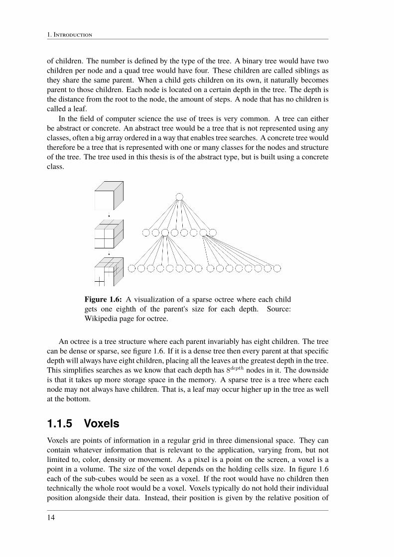
Figure 1.6: A visualization of a sparse octree where each childgets one eighth of the parent's size for each depth. Source:Wikipedia page for octree.

An octree is a tree structure where each parent invariably has eight children. The treecan be dense or sparse, see figure 1.6. If it is a dense tree then every parent at that specificdepth will always have eight children, placing all the leaves at the greatest depth in the tree.This simplifies searches as we know that each depth has 8depth nodes in it. The downsideis that it takes up more storage space in the memory. A sparse tree is a tree where eachnode may not always have children. That is, a leaf may occur higher up in the tree as wellat the bottom.

1.1.5 VoxelsVoxels are points of information in a regular grid in three dimensional space. They cancontain whatever information that is relevant to the application, varying from, but notlimited to, color, density or movement. As a pixel is a point on the screen, a voxel is apoint in a volume. The size of the voxel depends on the holding cells size. In figure 1.6each of the sub-cubes would be seen as a voxel. If the root would have no children thentechnically the whole root would be a voxel. Voxels typically do not hold their individualposition alongside their data. Instead, their position is given by the relative position of

14

1.2 R

other voxels, i.e. the position in the data structure that represents the three dimensionalvolume.

1.1.6 NoisePerlin noise was developed by the American professor Ken Perlin in 1983 and it is com-monly used today in the field if computer graphics when creating randomized behavioursor environments. The noise is a gradient type of noise which is most commonly imple-mented as a two, three or four dimensional function. Typically an implementation consistsof three steps: the grid definition, computing the dot product between the distance-gradientvectors, and finally interpolation between these values.

In 2001 Ken Perlin updated his original perlin noise and came up with the algorithmfor simplex noise. Simplex noise would tackle some limitations perlin noise has such asfewer directional artefacts, and in higher dimensions, computational cost. Some advan-tages simplex noise has over perlin noise:

• It is visually isotropic, it has no noticeable directional artefacts.

• Scales to higher dimensions (4D and 5D) with much less computational cost. Thecomplexity is O(n2) with n dimensions compared to O(2n) for perlin.

• Overall lower computational cost as it has fewer multiplications.

In this thesis we use simplex noise to simulate smoke in our volume.

1.2 Related workWe use a sparse octree that builds on the work of Brandon Pelfrey [11] but general overviewand information on how a sparse voxel octree functions and its details was found in thepaper ''Efficient Sparse Voxel Octrees'' [10] by Samuli Laine and Tero Karras. Here theycreate a world which only consists of voxels and no geometry. They showcase how theyorder their octree structure in a minimalistic way and how they traverse this in real-time.Their aim is to store representations of large-scale scenes in the GPU memory and focuseson representing surfaces instead of volumes. To enhance the details of their images theyadd contour data to allow accurate surface placement within individual voxels.

In the paper ''A Survey of Octree Volume Rendering Methods'' [8] the author, AaronKnoll, showcases different methods of volume rendering using octrees. He discusses thedifference in direct and non-direct volume rendering. The non-direct method was used inthe early days of volume rendering. Here they used the octree as a small memory footprintto extract a mesh pattern, triangles, from cells of volume. With this mesh they couldrender the volume as an isosurface. The direct method would be using the octree itselfas the volume and integrate the rays intersection with this. While this is slow for a CPUit can be effective on a GPU by accumulating gradients across sequential cutting planesof the volume, stored as two dimensional textures. This no longer restricts the volume tobe rendered as an isosurface. While it is faster on the GPU the bottleneck is the availablememory on the GPU. To bypass this, he states it is necessary to store the volume outsideof the GPU and page the data into the GPU's memory.

15

1. I

In this thesis we use the direct volume rendering method—there is no conversion ofthe octree data into another data type. The octree data is also constructed out-of-core, onthe CPU, and is sent into GPU memory.

Amanatides and Woo [1] were the first to present the regular grid traversal algorithm,used in octree traversal, that is the basis of most derivative work, including the used Rev-elles algorithm. The idea is to compute the t values of the next subdivision planes alongeach axis and choose the smallest one in every iteration to determine what next node theray pierces.

Knoll et al. [9] present an algorithm for ray tracing octrees containing volumetric datausing different isosurface levels. It proceeds in a hierarchical fashion by first determiningthe order of the child nodes and then processing them recursively. This is not well suitedfor GPU implementation.

Crassin et al. [2] introduces a voxel rendering algorithm for the GPU that combinestwo traversal methods. The first stage casts rays at an octree using a kd-restart algorithm toavoid the need for a stack. The leaves of the octree are not normal leaves but instead bricks.The bricks are three dimensional grids that contain the voxel data. When a brick is reachedthe data is sampled. Bricks does not contain a single value but instead values of 163 or323 voxels. This yields a lot of wasted memory if the data is not truly volumetric or fuzzy.However, three dimensional lookups supported by the hardware make the brick samplingefficient, with the bonus of the result being automatically anti-aliased. This algorithm alsosupports data managements between the CPU and GPU. While traversing the octree, thealgorithm detects if there is data missing in the memory of the GPU. If so, the algorithmsignals to the CPU that data is missing and the CPU then streams the missing data to theGPU. This feature enables that only a subset of data needs to reside in the GPU memory.

The traversal of our octree is mainly based on the paper by J. Revelles. et al. [14] withsome modifications regarding the children indexes.

The noise creation is based on the works of Eliot Eshelman [3] where he describes away of computing simplex noise in a simple fashion for both C++ and Python.

1.3 Problem and contributionThe issue we are trying to address in this thesis is an issue of optimization. When sam-pling volumetric data in a volume using a standard medium as the container, e.g. a threedimensional texture, one may sample huge volumes of empty space. This empty spacecontains no real informations describing the actual volume we want to render, therefore awaste in computational power.

To tackle this we introduce an alternative medium to hold the volumetric data—anoctree. This will enable us to mark out the empty space in the volume and skip past allthis when sampling. That is, we do not sample empty space, only values that represent thereal volume.

1.4 Report structureIn the beginning of chapter 2 we first describe the overall layout of the implementation.We then go more into details of each key stage of the implementation. In chapter 3 we

16

1.4 R

show the result of our implementation, both in numbers and visually. This is followed upby a discussion in chapter 4 and finally a conclusion is given in chapter 5.

17

1. I

18

Chapter 2Implementation

On the GPU we implement a ray marcher engine with support for distance fields, phongshading (basic light calculations that gives highlights on objects), the octree traversal al-gorithm and support for using three dimensional textures. This was done with a computeshader using GLSL version 4.5.

Outside of the shader, on the CPU using C++, we first calculate the noise that is usedto fill our three dimensional texture and octree. Then we go through the octree to retrievethe octree array. This array is used by the traversal algorithm, inside the compute shader,when traversing the octree in real time. The array represents a linear one dimension datastructure of the three dimensional octree. This enables us to to make fast indexing whentraversing. The three dimensional texture along with the array is sent to the shader and islater used when sampling the volume.

In the shader we ray march each pixel. Depending on what we hit we calculate thecolor for this pixel. When the color is determined we write the color to an empty texturethat is bound to the shader. This texture is then sent through the regular graphics pipelineto be displayed on our screen.

The octree and the three dimensional texture are comparable as they both represent thesame volume. In the case of the texture, it only holds points in a non-ordered structure,apart from the order we enter our noise. It also does not distinguish empty space fromnon-empty. The octree orders the smoke in a more hierarchical way utilizing the nodesposition, (x, y, z), in regards to each other and will not include empty space more thansaying there is nothing here.

2.1 Full screen quadTo get an image from our compute shader we have to bind our texture that comes from theshader to a buffer—a container to store the texture in memory. This buffer is called the fullscreen quad and can be seen as the quad where we will paint our image on. The quad is

19

2. I

constructed using a float array containing the four corner coordinates of the screen. Thesecoordinates are then used to create two triangles that will be used when drawing the finalimage, see figure 2.1.

Figure 2.1: A full screen quad. The coordinates represent theOpenGL window coordinates.

For each cycle we will call the renderScene() function and run a compute dispatch onour compute shader. We bind an empty texture to it that is the size of our window, inthis case 1024 x 768. The compute shader will ray march each pixel in the window andwrite the resulting color to the appropriate place in the texture. When the texture is filledwe bind this to our screen buffer and proceed with showing it as a normal texture in thefragment shader using the float array as texture coordinates.

2.2 NoiseTo construct our noise we loop over each dimension, x, y and z, where x, y, x ∈ (0, res),res being the resolution of the noise. For each combination of coordinates we call thenoise function:

float noise = scaled_octave_noise_3d(octaves,persistence,scale,lowBound,highBound,x, y, z);

This function takes a number of parameters and scales the final noise value from [−1, 1]to [lowBound, highBound]. For each iteration in the noise function a higher frequencyand lower amplitude function will be added to the original base function. The persistence,[0, 1], sets how much of the last octave will be added. A higher persistence will includemore from each octave. Scale sets the frequency of the noise.

In this thesis we use the parameters scaled_octave_noise_3d(8, 1, 0.0015, -70, 400,x, y, z) . The reason why we scale it past the max value of 255 and below 0 for colors is

20

2.3 C

simply to spread out the noise, making more empty space in our smoke. In addition, wedo not include noise values below 255 either. This is because we want even more space,but also because higher resolutions of noise would reach the max amount of memory theapplication could use when creating the octree. The project was conducted using VisualStudio Ultimate 2013 and by default every project was set to run in 32-bit mode. Enablinglong addresses in the application will however increase the available memory to about4GB. If the project would have been built in a 64-bit environment the memory issue wouldnot be as much of a limit.

2.3 Constructing the octreeThe octree is implemented with help of two classes. The octree class is the main classcontaining tree operations such as inserting and initialisation of the tree. The other classis the octreePoint class which is a simple class that represents a point in the tree. Thisclass has attributes for holding the noise value and its own position and also retrieving thisposition. The octree class holds information about its center, its half dimension, childrenand an octree point. The half dimension parameter is the distance from the origin and out-wards of the current node. For example, setting the root's origin to 0 and its half dimensionto (2, 2, 2) would yield a root node spanning from (-2, -2, -2) to (2, 2, 2) with a size of 43.

To create a tree we first invoke the tree class' constructor, setting the origin of thetree, its half dimension and setting all the children and its octree point equal to null. Thechildren follow a simple pattern in which the nodes are placed. Plus means that the positionin that dimension is greater than the origin of this node, minus indicates less than. A visualrepresentation can be seen in figure 2.2. For each noise value we generate we insert it intoour tree as a node.

Child: 0 1 2 3 4 5 6 7x: - - - - + + + +y: - - + + - - + +z: - + - + - + - +

When inserting a new node in the tree we must first consider three cases:

1. The node is an interior node, it has eight children.As parents never store data themselves we find out where in its eight children this newnode would be positioned and make a recursive call to insert into that child's position.

2. The node is a leaf, it has no children and its data is equal to null.We are in a region where there is no data, store the noise data here.

3. The node is a leaf but its data is not null.Save the current node temporarily, split the current node into eight children and insert thetemporary and the new node into the new children. This may happen several times if thepoints tend to lay close to each other.

21

2. I

Figure 2.2: Child order in the octree.

To calculate at what index position in the children the new node would go, we use abitwise OR operation. Given the new node's coordinates we check each dimension againstthe origin of the current node in regards to the layout pattern given above:

int oct = 0;if (point.x >= origin.x) oct |= 4;if (point.y >= origin.y) oct |= 2;if (point.z >= origin.z) oct |= 1;return oct;

A pseudo code of the octree creation algorithm can be seen in algorithm 1.

22

2.3 C

Initialize tree;input : An octree pointwhile has input do

if isLeafeNode thenif data == NULL then

data← point;else

/* We are at a leaf but there is already datahere, split the node and insert recursively.*/

oldPoint← data;data← NULL;for i← 0 to 8 do

newOrigin← origin;newOrigin.xyz← calculate new dimensions;children[i]← new octree(newOrigin, halfDimension · 0.5f );

end/* Re-insert old and new point. */children[getOctantContainingPoint(oldPoint)]→ insert(oldPoint);children[getOctantContainingPoint(point)]→ insert(point);

endelse

children[getOctantContainingPoint(point)]→ insert(point);end

endAlgorithm 1: Octree creation.

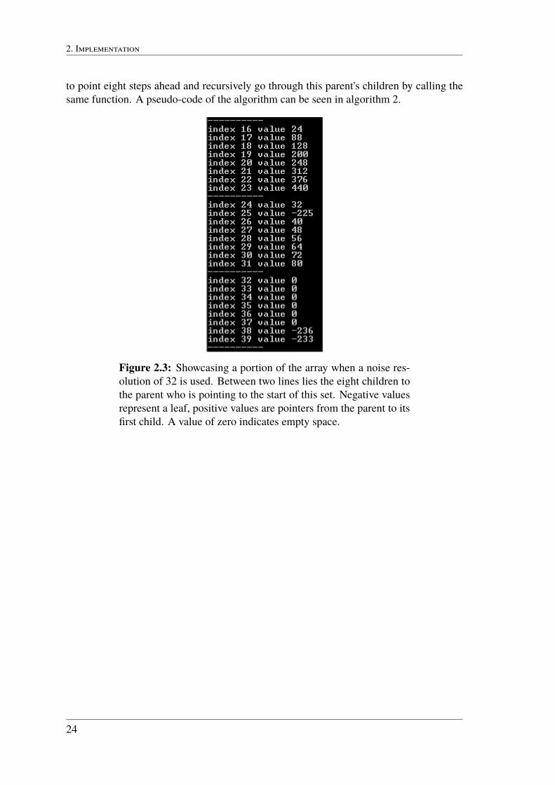
2.3.1 The octree arrayWhen the tree is built we need to construct our array so we can send this to our computeshader. To do this, we traverse our tree, starting at the node in a depth-first fashion. Thearray will not include the root, the first level of the volume, as this is redundant. Eachparent will have eight slots in the array. A parent whose any of its children have data inthem, either as a leaf or another parent, is given a positive number that is the index in thearray where the start of its eight children is. Leafs have negative numbers and empty spaceis represented as a zero. An array constructed with a low resolution noise can be seen infigure 2.3.

When invoking the function we suffice it with an empty array of the type vector, thatwill become the octree's array. We start at the root, first checking so that its child at indexzero is not NULL. If so, we push the root value and return the list. If not, we begin ourdecent. First we count this node's active children, which can be either leaves or otherparents, and keep track of what index they have. As a vector array does not have a variablesize it is necessary to change its size as the number of values grows. We resize our vectorby plus eight and iterates over the active children. If this child is a leaf, we extract its noisevalue and insert it in the array at the right index. If not, we set this index in the array

23

2. I

to point eight steps ahead and recursively go through this parent's children by calling thesame function. A pseudo-code of the algorithm can be seen in algorithm 2.

Figure 2.3: Showcasing a portion of the array when a noise res-olution of 32 is used. Between two lines lies the eight children tothe parent who is pointing to the start of this set. Negative valuesrepresent a leaf, positive values are pointers from the parent to itsfirst child. A value of zero indicates empty space.

24

2.4 R

input : int localIndex, int& treeIndex, vector<int>& treeResultsoutput: A filled treeResults arrayInitialize: localIndex← 0, treeIndex← 0;localIndex← treeIndex;if children[0] == NULL then

push-back value and return;endcreate activeChildren array;for k← 0 to 8 do

if children[k] is active thenactiveChildren← k;

endendresize treeResult by 8;for i← 0 to activeChildren.size() do

childIndex← activeChildren[i];if children[childIndex] is a leaf then

treeResult[localIndex + childIndex]← value of leaf;else

treeIndex← treeIndex +8;treeResults[localIndex + childIndex]← treeIndex;children[childIndex]→ getArray(localIndex, treeIndex, treeResults);

endend

Algorithm 2: Array retrieval algorithm.

2.4 Ray marchingTo be able to ray march we first need to define our ray:

r(t) = (xo, yo, zo) + (xd, yd, zd) · t (2.1)

or in short:r(t) = o+ d · t (2.2)

where o is the origin of the ray, our camera, and d is the direction of the ray. t is a scalarused to step along the ray. A positive t moves us towards the scene while a negative wouldmove us behind the camera. For ray marching one often sets a constant maximum amountof steps to take before considering this ray to not have hit anything. If the maximumnumber of steps are too low it might result in artefacts between objects. If it is too highthe computational cost would be too great, risking losing frames per second. In this thesiswe define a variable called MAXSTEPS that tells us how many steps are allowed to betaken on the ray. This variable is calculated from the volume's size and the length of thesteps we take in the volume. The code below shows the calculations made to computethe MAXSTEPS variable. volumeStepSize is the step length we take in the volume whensampling. h1 is the hypotenuse of the bottom plane in the volume. maxSteps is the diagonal

25

2. I

in the volume. The multiplication of 3.2 is just to increase the amount of steps a bit furtherto eliminate artefacts.

const float volumeStepSize = 0.1;float volumeScale = VOLUMESIZE / volumeStepSize;float h1 = sqrt(volumeScale * volumeScale + volumeScale * volumeScale);int maxSteps = int(sqrt(h1*h1 + volumeScale * volumeScale)*3.2);#define MAXSTEPS maxSteps

As we fire our ray from our camera through our imaginary plane and into the scene, foreach point we measure the distance between two objects. The first object is the volume,represented as a cube. The second is the platform beneath the cube, represented as aflattened cube. The shortest of these distances is denoted dist. To check if we hit anobject we check dist against a threshold called EPSILON. This threshold has the value of0.0005 and indicated that we have to march along the ray until be are below this to ensurea hit. As we are running a variable step size we multiply this EPSILON by the scalar t. Ifwe are not within the threshold we increase t by dist. If we hit the platform beneath weapply a simple phong shader to it that interacts with our movable light source in the scene.

If we are running the three dimensional texture and we hit the volume we stop usinga variable step size and instead sample at a constant step size of 0.1. If this value is toogreat we might risk oversampling the texture which from some angles will give visualartefacts. If the value is too low we might risk sampling the same thing multiple times,with an increase in computational power. If we are running the octree we instead invokethe traversal algorithm. This enables us to skip the empty space and only sample the actualdata, see figure 2.4 for the difference in the two data types.

2.4.1 Traversing the octreeThe octree is traversed using a loop and a stack. On the stack we save, for each nodewe enter, parameters for entry and exit points in all dimensions, the current node we arestanding in varying from 0 to 7, the node index we are standing in in the tree array and thelength dimensions. The stack is ordered as an array where each of the named variablesare grouped as a struct. The struct is accessed with a stack pointer, telling us where inthe array we are. In the loop we check which child index we are piercing and enters thatnode's sub-tree. When so the stack pointer increases by 1. If we hit or exit a node the stackpointer gets subtracted by 1. The loop is continued as long as we are not leaving the stack,checking if the stack pointer is < 0.

When hitting the volume with the octree enabled we first initiate the entry and exitvariables used by the algorithm. These are based on the origin and direction of the ray.The algorithm only works for positive ray direction. If we encounter a negative ray in anydimension we invert its direction and position in that dimension. We also set one of threevariables a, a2 or a4 to either 1, 2 or 4 depending on if it was the z, y or x direction that wasinverted. These will be used to modify the child index to enter as the algorithm assumes achild order in the tree that is mirrored in the z-axis in regard to the order of the built tree.If a ray direction is equal to 0 we substitute this by 0.00001 to eliminate division by zero.

26

2.4 R

Figure 2.4: Difference of how the two data structures are sam-pled. The orange dots are the sampling points, the purple crossesare operations in the octree. In the texture we take small stepsthroughout the volume, even if we hit empty space—the white ar-eas. In the octree we instead see that this area is empty and thusskip this region and only sample the valid data, the noise—the blueregion.

To initiate the values of the root node we calculate the entry and exit point for the nodein each dimension using slabs. These points will be used throughout the algorithm to de-cide which node we would hit next as we pierce the volume. A slab can be seen as a planeeither spanning the XY, XZ or the YZ plane. To get the entry and exit point we checkthe intersection of two slabs in each dimension, think of it as two planes on each side of acube. A two dimensional example in the x dimension is given in figure 2.5. The principalfor three dimensions is the same.

To calculate the entry point, txmin, we use:

txmin = (xmin − ox)/dx (2.3)

and the exit point, txmax, is similarly given by:

txmax = (xmax − ox)/dx (2.4)

The calculations of the six intersection points will be passed down the algorithm aswe descend the structure and enter smaller and smaller cubes. But before we do that we

27

2. I

Figure 2.5: A two dimensional slab intersection. o is the originof the ray and d its direction. xmin and xmax are the cube's minand max value of x. txmin and txmax are the intersection points ofthe two slabs.

calculate the distance this ray is travelling in the volume, the root, by taking the distancebetween the exit and entry point. tx1 would translate into txmax and so forth.

float r = min(min(tx1, ty1), tz1) + 1;float e = max(max(tx0, ty0), tz0) - 1;

float res = r - e;return res;

The ±1 is there to give some margin against errors, otherwise we risk artefacts in thevolume.

After all the variables have been initiated we begin our descent. We check which indexof the root's children we first pierce with our ray and enters it. When we reach a node inthe tree we check for four different cases:

1. Are we leaving the current node?We do this by evaluating if any of the most positive slab exits are less than zero, i.e. if tx1,ty1 or tz1 is negative. If so, we go up one step in the algorithm and proceed to process thenext node in line.

28

2.4 R

2. Hit empty space?If this node's value is zero then it represent empty space. If so, go back one step and pro-cess the next node in line.

3. Is it a leaf?If the value of the current node is negative this indicates that we have hit a leaf. If so,we use the same method as described above to get the distance this ray is travelling in thenode. This is weighted with the nodes' noise value. Thereafter we go up one step andcontinue our traversal by processing the next node in line.

4. We hit a parent.When so, we calculate the point that lies between max and min of each dimension by mul-tiplying their sum by 0.5 and call these tim where i ∈ (x, y, z) We save these plus thenode and the exit and entry points to the stack and call a function to see what plane of thenew node we would hit with our current exit and entry point. This is done by comparingtim with the entry points. For example, if we enter the XY plane we know that the raywould either enter node number four, two or six. When knowing what index we first enterwe go down this sub-tree and continue our traversal.

By doing this we check each node that is intersected by our ray in the octree. Whenall the nodes that are intersected have been evaluated we have accumulated a noise valuethat we integrate with the scene behind the volume. If the value reaches over 1 in any stateof the traversal we exit and call this a saturated smoke value that is to be coloured in thesmoke's color with no transparency. After the traversal we instantly step past our volumeand proceed to march as normal.

29

2. I

30

Chapter 3Results

3.1 MeasurementsTo test the implementations we measure the frames per second (FPS) of our applicationin various camera positions. We compare the traversal of the octree with the samplingfrom the three dimensional texture. The resolution of the smoke varies from 32 units upto 512 units and for each resolution we measure octree build time and array build timein seconds. We also measure the size of the array and the number of elements we skipdue to too low noise value. The resolution of our windows is 1024 x 768. The tests wereconducted on a computer with an Intel Xeon E5-1620 3.50GHz CPU, 64GB of memoryand a Radeon HD 7970 with 4GB of video memory by AMD. The time was measuredusing the function glutGet(GLUT_ELAPSED_TIME) before and after the code snippetmeasured. The difference of these two values is taken and divided by 1000. The FPS wasmeasured in a similar fashion with addition of a frame counter that we increase each timethe renderScene() function ended.

In table 3.1 we can see the construction time of the octree and the array, the size of thisarray—how many elements it contains, and the number of skipped noise values due to thevalue of the noise being too low.

Resolution 32 64 128 256 512Octree(s) 0.126 0.947 6.802 48.855 334.720Array (s) 0.145 3.736 9.832 39.020 853.710Array (size) 27 352 189 312 1 125 912 5 031 160 18 436 176Elements skipped 14 649 140 958 1 426 183 14 068 363 125 195 663

Table 3.1: Build time in seconds, size of the array and number ofskipped elements in different resolutions.

Table 3.2 shows the average FPS in the various resolutions. We also compare FPS in

31

3. R

the resolution 128 when we change the size of the volume. That is, we increase the x, yand z dimensions of our cube that holds our volume, making it physically bigger, see figure3.6, 3.7 and 3.8. The standard size of the volume is 8.

Resolution 32 64 128 128 VS 16 128 VS 32 128 VS 64 256 5123D texture 111 111 111 59 27 13 111 111Octree 30 14 9 6 4 3 4 2

Table 3.2: Average FPS in different resolutions. VS stands forvolume size. The standard volume size used is 8.

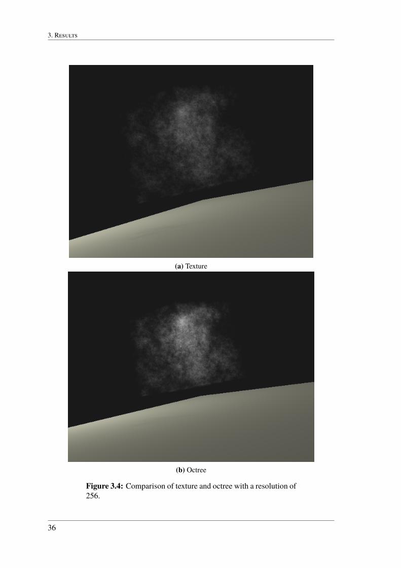
3.2 Visual comparisonWe see some tiny differences between the two versions. The most noticeable difference isthe saturation of the two versions—the difference in thickness of the smoke. At the lowerresolutions, see figure 3.1 and 3.2, there is almost no difference i saturation. When weincrease the resolution to 128 and above, see figures 3.3, 3.4 and 3.5, we see that the twoversion start to sample differently. In this case we are undersampling the texture. Figure3.6, 3.7 and 3.8 showcases the difference when the size of the volume increases. Here wecan see that the texture is oversampled compared to the octree.

The shadow below the noise is only sampled from the three dimensional texture, evenif the octree version is running. The shadow can be controlled in real-time by movingthe light source—also changing the appearance of the platform which is rendered using aphong shader.

32

3.2 V

(a) Texture

(b) Octree

Figure 3.1: Comparison of texture and octree with a resolution of32.

33

3. R

(a) Texture

(b) Octree

Figure 3.2: Comparison of texture and octree with a resolution of64.

34

3.2 V

(a) Texture

(b) Octree

Figure 3.3: Comparison of texture and octree with a resolution of128.

35

3. R

(a) Texture

(b) Octree

Figure 3.4: Comparison of texture and octree with a resolution of256.

36

3.2 V

(a) Texture

(b) Octree

Figure 3.5: Comparison of texture and octree with a resolution of512.

37

3. R

(a) Texture

(b) Octree

Figure 3.6: Comparison with a resolution of 128 and a volumesize of 16.

38

3.2 V

(a) Texture

(b) Octree

Figure 3.7: Comparison with a resolution of 128 and a volumesize of 32.

39

3. R

(a) Texture

(b) Octree

Figure 3.8: Comparison with a resolution of 128 and a volumesize of 64.

40

Chapter 4Discussion

The construction time of the octree and its array is hardly noticeable in the lower reso-lutions, 32 and 64, with a total time varying from 0.271 to 4.683 seconds. As soon asthe long addresses is utilized, we increase the resolution, the time increases drastically byabout a factor of eight for each increase. The time it takes to construct the array is almostin every case slower than construction the tree itself. This is because the tree construc-tion algorithm never restarts at the root node for each insert. The array construction usesa depth first approach and therefore is forced to go through every node in the tree, plussome internal list iterations. With the chosen algorithm for building the tree it is not morebeneficial to try and construct the array at the same time as the tree is constructed. This isbecause we split nodes during construction and re-insert the old together with the new one,reordering the tree multiple times during building. We also notice that the size of the arrayplus the number of elements skipped is greater than the resolution cubed. This is becausewe include zeroes in the array size, representing the empty space in that region of the tree.As the resolution gets higher the majority of the points get removed due to too low noiselevel. This is intended as we want more empty space to showcase possible speed bene-fits. But as we can see, the frames per second when using the octree is nowhere near thevalues when using the three dimensional texture. This is because the traversal algorithmused contains a non dynamically uniform flow-control sequence. To explain this we haveto mention the difference in branching between CPUs and GPUs as the paper of Revellesalgorithm, the algorithm used for traversing the octree, was only evaluated on the CPU.

To obtain high performance on modern CPUs they are all pipelined. This means thatthey consist of smaller parts that may partly process an instruction and send the result tothe next stage in the pipeline. After they sent their result they immediately start on thenext instruction. Obviously, this requires the knowledge of what instruction to processnext. If we have a purely linear program this is not hard to predict, just take the next lineof code. But by having a branch that is based upon a condition, that in some cases mightbe variable (non uniform), makes it impossible to know which instruction to process next.To fix this we either program in a branch-less manner or we rely on the CPUs ability to

41

4. D

apply branch predictions. A branch prediction is simply a guess based on the condition toeither go down path a or path b. As a CPU generally has deep pipelines, it is imperativeto be able to accurately predict whether a branch might be taken or not. If its predictionis successful the penalty for branching is often just minor. If it fails, the CPU stalls someclock cycles, flushes the pipeline and refills with the correct address. Depending on thesize and complexity of the different branches, the overall cost for this is not that grave.

The GPU handles this differently. As we recall, compute shaders invoke several par-allel threads to run their code. This is favourable as a GPU is made for massive parallelexecutions. There are many shader cores running asynchronously and each core can runmultiple threads. This all functions well as long as we are executing the same code at thesame time within a core. When we do the opposite, creating a conditional branch, the GPUhas to decide what to do. We have created a situation where threads within a core, depend-ing on the condition, execute different instructions and may therefore have diverged fromthe rest of the core's threads. A GPU does not have branch predictions. Instead, when thishappens the GPU utilizes the single instruction multiple data (SIMD) control mechanism.What this means is that when multiple threads diverge within a core the GPU halts everythread that is not taking this branch. After the threads that took the branch have finished,the GPU in series run the remaining threads that did not take the branch. This means thatin worst case the GPU runs all the branches in series after one another, taking as longtime as all the branches combined. The SIMD works well when we have fewer coherentbranches, but for many incoherent branches the result can be expensive. This is a generalapproach and its effectiveness is highly dependent on the type of graphics card used andimplementations of such control mechanisms. [12]

Unfortunately the traversal algorithm chosen appears to be very divergent. As soon asthe loop for the traversal became non dynamically uniform we instantaneous lost about 40FPS. This was noticed during testing when we first observed the drop in FPS. We triedto only fill half of the volume with smoke to see if it made any difference. There was nodifference in the FPS. Even with a complete empty volume the drop in FPS was there.When limiting the amount of times the loop could run we noticed that it usually runsbetween 100 and 250 times, depending on the resolution. This seemed ok but even if thelimit was set to 1 the drop in FPS was there. We might have gained a few FPS by limitingthe loop to 1 but not near the lost 40. So our conclusion were that the low FPS were notconnected to the amount of times the loop was running, instead that the loop became nondynamically uniform. We tried to change the algorithm and rework its flow in many ways.By setting the used stack as shared would give us back almost all the FPS, but anotherproblem arose. The smoke would appear pixelated and flicker a lot. This is because thethreads were not synchronizing the use of the stack. But a second problem occurred.

As we explained in the compute shader section, 1.1.2, to be able to synchronize theuse of a the shared stack we have to have a dynamically uniform flow-control. As thealgorithm itself is relying on going down different sub-children, depending on what childindex one stands in right now, and changing this index in the sub-routines, the nature of thisalgorithm's flow-control is non uniform. If we had a dynamically uniform algorithm, notonly could we gain back the lost 40 FPS, but we could also set the stack to shared, gainingadditional FPS. We believe using a different traversal algorithm, either a stack-less one oran algorithm with much less branching, would heavily benefit the speed at which we canrender a frame.

42

Visually the two types look almost the same shape-wise. There are some differencesin the lower resolutions that is worth noting. When we have a single point in the volumewith nothing around it the texture would display this as a tiny area of smoke, but in theoctree this would show as a large cube. This is because there is no other data around thissingle point, or too few, pushing this node further down the tree. This difference gets lessnoticeable when increasing the resolution.

Even though we scale the amount of noise we pick up in regards to the volume sizeit is hard to get these two version alike. Overall we think that the octree represents themore accurate noise value picked up. This scaling can be observed by comparing theresolution of 128 and 256, seen in figure 3.3 and 3.4. As we pack more data into thevolume, while maintaining its size, the traversal of the octree will always pick up everysingle node that the ray crosses and their respective noise value. For the three dimensionaltexture it could happen that the data points get so packed that we unintentionally skip somevalues, undersampling.

When changing the size of the actual volume we observe that the saturation of the noiseis affected in the texture, see figures 3.6, 3.7 and 3.8. Here we see a case of oversamplingin the texture. This effect gets more and more pronoun as the volume grows. Meanwhile,we can observe a constant saturation in the octree, regardless of the size of the volume.We could have tried to implement a variable step size for the texture depending on thesize of the volume. But the main problem still remains, it is very hard to know if we areover- or undersampling. Besides the ocular measurements one could try to measure thedifference using a picture comparison program. This will then calculate how much thetwo pictures actually differ per pixel by comparing its color. However, this might not yielduseful numbers. For this to work we have to make sure that the texture samples each valueonly once—neither under- nor oversampling. This is extremely hard to check as we haveno boundaries in the texture itself. Even if the two pictures look exactly alike, there mightstill be difference in the actual noise value for each pixel. This will give a false reading assoon as the values only differ by one or more units.

The FPS with the texture stays the same independent of the resolution. This is logical aswe still take the same amount of steps in the volume. For the octree, with higher resolutionscomes longer traversals, thereby change in FPS. By doubling the volume we loose about50% of our FPS in the texture and about 30% with the octree. By increasing the size evenfurther we still halve our FPS for each step, although the octree is affected less by the sizedifference. The small difference in FPS for the octree could be the small difference incamera positions. If we would have exactly the same amount of pixels of smoke for boththe texture and the octree, regardless of the size, the octree would not loose any FPS as theresolution is the same. The number of steps in the texture would however increase.

43

4. D

44

Chapter 5Conclusion

The goal of this thesis was to see if traversing an octree in real-time with a lot of emptyspace would be faster than sampling a three dimensional texture. The results show thatwith the chosen traversal algorithm it is not, independent of the amount of empty space inthe volume. This is because the algorithm is non dynamically uniform. The octree doeshowever scale better in speed when the resolution of the noise stays the same but the volumesize increases. It also has more accurate noise saturation than the texture. Therefore thevisuals look better with the octree, with some differences on lower resolutions. The buildtime and memory consumption when building the octree and its array is reasonable forlower and medium resolutions. The project might benefit to have been build in a 64-bitversion, eliminating the memory limit. Furthermore, if we would have used a traversalalgorithm that is dynamically uniform the speed of the octree would most likely surpassthe speed of the texture. Enabling the stack to be shared would probably yield even greaterspeed gains. With these improvements we are sure this approach of rendering volumes willbe viable in real-time applications.

45

5. C

46

Bibliography

[1] John Amanatides, Andrew Woo, et al. A fast voxel traversal algorithm for ray tracing.In Eurographics, volume 87, page 10, 1987.

[2] Cyril Crassin, Fabrice Neyret, Sylvain Lefebvre, and Elmar Eisemann. Gigavoxels:Ray-guided streaming for efficient and detailed voxel rendering. In Proceedings ofthe 2009 symposium on Interactive 3D graphics and games, pages 15--22. ACM,2009.

[3] Eliot Eshelman. Simplex noise. http://www.6by9.net/simplex-noise-for-c-and-python/ [Accessed 25 May 2015].

[4] Khronos Group. Compute shader. https://www.opengl.org/wiki/Compute_Shader [Accessed 25 June 2015].

[5] Khronos Group. Core language opengl. https://www.opengl.org/wiki/Core_Language_%28GLSL%29#Dynamically_uniform_expression[Accessed 25 June 2015].

[6] Khronos Group. Memory barriers. https://www.opengl.org/wiki/Memory_Model#Ensuring_visibility [Accessed 31 August 2015].

[7] Khronos Group. Shader storage buffer object. https://www.opengl.org/registry/specs/ARB/shader_storage_buffer_object.txt[Accessed 25 June 2015].

[8] Aaron Knoll. A survey of octree volume rendering methods. Scientific Computingand Imaging Institute, University of Utah, 2006.

[9] Aaron Knoll, Ingo Wald, Steven Parker, and Charles Hansen. Interactive isosurfaceray tracing of large octree volumes. In Interactive Ray Tracing 2006, IEEE Sympo-sium on, pages 115--124. IEEE, 2006.

[10] Samuli Laine and Tero Karras. Efficient sparse voxel octrees. In Proceedings of the2010 ACM SIGGRAPH Symposium on Interactive 3D Graphics and Games, I3D '10,pages 55--63, New York, NY, USA, 2010. ACM.

47

BIBLIOGRAPHY

[11] Brandon Pelfrey. Coding a simple octree. http://www.brandonpelfrey.com/blog/coding-a-simple-octree/ [Accessed 28 Mars 2015].

[12] Matt Pharr and Randima Fernando. GPU Gems 2: Programming Tech-niques for High-Performance Graphics and General-Purpose Computation (GpuGems), chapter 34. GPU Flow-Control Idioms. Addison-Wesley Professional,2005. http://http.developer.nvidia.com/GPUGems2/gpugems2_chapter34.html.

[13] Iñigo Quilez. Distance functions. http://www.iquilezles.org/www/articles/distfunctions/distfunctions.htm [Accessed 02 Mars2015].

[14] J. Revelles, C. Ureña, and M. Lastra. An efficient parametric algorithm for octreetraversal. In Journal of WSCG, pages 212--219, 2000.

48

Dagens datorgrafik strävar ständigt efter att skapa mer verklighetstrogna bilder. För att kunna lägga in fler detaljer i bilden måste vi förbättra det sätt vi gör det på. Således testar vi ett alternativt sätt att rita upp rök i en dator snabbare.

InledningFör att på ett snabbare sätt kunna rita verklighetstrogna bilder med grafikkortet i en dator så är det viktigt att förbättra, optimera, denna process. Man vill med andra ord förkorta den tid det tar att rita en bild. Desto mer man kan rita upp på kort tid, desto detaljrikare kan bilderna bli. Utan optimering så kan bildsekvenserna upplevas som sega och de tenderar att släpa efter. Vid simulering av rök eller då man exempelvis skall visualisera bilder från en magnetröntgen använder man sig av volymer när man ritar bilderna i datorn. En volym kan anta olika former av tredimensionella kroppar. En enkel och vanlig form är en kub. I kuben finns data som representerar den volym man vill rita. Det är väldigt krävande att låta datorn rita volymer och därför är optimering av sådana processer av stort intresse.

Ray marchingNär man ritar volymer så använder man sig av en teknik som heter ray marching. Tänk dig att du tar en bild med en vanlig kamera och från ditt öga så skjuter du ut strålar. Varje stråle träffar och går igenom en punkt på fotot du tänker ta. Strålen fortsätter genom fotot och ut i verkligheten och träffar det du vill fotografera. Beroende på vad strålen träffar så blir denna punkt som strålen gått igenom färgad olika. Tänk dig nu att när vi skjuter en stråle så hoppar vi också fram på denna med små steg. För varje steg vi flyttar oss framåt på strålen så kollar vi om vi har träffat nått. Detta är konceptet för ray marching.

ProblemNär vi träffar vår volym så börjar vi ta ännu mindre steg genom hela volymen. För varje litet steg vi tar så hämtar vi information från volymen om hur röken ser ut just här för denna stråle. Finns det ingen information att hämta här, volymen är tom, så försöker vi ändå hämta den. Detta är slöseri med beräkningskraft och vi vill i stället försöka optimera detta så att vi inte behöver hämta information som ändå inte ger oss någonting.

LösningFör att möjliggöra en optimering byggs en trädstruktur, ett så kallat octree, upp av röken. Med hjälp av denna struktur kan vi dela in volymen i bitar. Dessa bitar kan då säga oss om det finns information här som vi kan använda. Är det tomt, så talar vårt octree om det för oss och hoppar då förbi allt detta tomrum direkt. Därmed kan vi spara beräkningskraft.

Resultat Resultaten visar att metoden har potential, men det sätt vi frågar vårt octree på omöjliggör en optimering. Detta beror på hårdvarubegränsningar i dagens grafikkort som grundar sig i dess oförmåga att förutspå och hantera komplexa förgreningar av kod. Octree:t ger dock ett mer noggrant värde av röken då vi varken hämtar för mycket eller för lite information om den i volymen. Detta resulterar i en mer visuellt korrekt återgiven rök.

EXAMENSARBETE Real-Time Volumetric Lighting Using SVOs

STUDENT Victor Strömberg

HANDLEDARE Michael Doggett (LTH)

EXAMINATOR Flavius Gruian

Att rita rök snabbare på en datorPOPULÄRVETENSKAPLIG SAMMANFATTNING Victor Strömberg

INSTITUTIONEN FÖR DATAVETENSKAP | LUNDS TEKNISKA HÖGSKOLA | PRESENTATIONSDAG 2015-08-28