VIBRO Software Experimental Validation - Defence...

Defence R&D Canada

DEFENCE DÉFENSE&

VIBRO Software Experimental Validation

Alain BerryJean-Luc WojtowickiSamuel BerryRaymond PannetonDepartment of Mechanical Engineering

Department of Mechanical EngineeringUniversity of SherbrookeSherbrooke, QuebecJ1K 2R1

Contract Number: W7707-008313/001/HAL

Contract Scientific Authority: J.P. Szabo, Ph.D., (902) 426-0550 ext. 3427

Contractor Report

DREA CR 2001-054

July 2002

Copy No.________

Defence Research andDevelopment Canada

Recherche et développementpour la défense Canada

This page intentionally left blank.

Copy No:

VIBRO Software Experimental Validation Alain Berry Jean-Luc Wojtowicki Samuel Berry Raymond Panneton Department of Mechanical Engineering University of Sherbrooke Sherbrooke, Quebec, Canada J1K 2R1

Contract Number W7707-008313/001/HAL Contract Scientific Authority J.P. Szabo, Ph.D. Defence R&D Canada – Atlantic P.O. Box 99000 Stn. Forces Bldg D-17 Halifax, NS B3K 5W5 (902) 427-0550 ext. 3427

Defence R&D Canada – Atlantic Contractor Report DREA CR 2001-054 July 2002

Abstract The University of Sherbrooke's Acoustics and Vibration Group (GAUS) have developed a computer code called VIBRO for modelling the effect of damping and decoupling coatings on the sound radiation from fluid loaded plates. In this work, laser vibrometry was used to measure the vibration on the both the wet and dry sides of plates backed by a water filled cavity. VIBRO accurately predicted the mean square velocity spectra of bare 2 mm steel plates in air, both in terms of peak positions and magnitudes. The agreement between experimental data and VIBRO model predictions was not quite as good for the corresponding experiment of the bare plate in water, but peak positions still matched closely. A modified Oberst beam method was used to determine the complex Young's and shear modulus of four different types of foam materials: 3 mm neoprene, 6 mm ethylvinylacetate, 12 mm ethylvinylacetate, and 25 mm EPT/SBR foam. For plates coated with these foams, the VIBRO model predictions were generally very good on the water side of the plate. However, the VIBRO model calculations did not capture a dip in the mean square velocity spectum that was observed on the air side of coated plates. The results suggest that VIBRO is a useful tool for prediction of the vibration insertion loss and acoustic insertion loss as vibroacoustic indicators. The experimental results related to the effect of the decoupling coatings on the vibration at the plate/ air interface could not be explained in terms of the VIBRO model.

Résumé Le Groupe d’acoustique de l’Université de Sherbrooke (GAUS) a mis au point un programme informatique appelé VIBRO servant à modéliser les effets des revêtements d’amortissement et de découplage sur les radiations acoustiques imputables à des plaques chargées de fluides. Dans ces travaux, on a eu recours à la vibrométrie laser pour mesurer les vibrations sur les côtés humides et secs de plaques reposant sur une cavité remplie d’eau. Le VIBRO a permis de prévoir avec précision les spectres de la valeur quadratique moyenne de la vitesse de plaques d’acier non revêtu de 2 mm d’épaisseur dans l’air, en termes de positions et d’amplitude maximales. La concordance entre les données expérimentales et les prévisions du modèle VIBRO n’a pas été aussi bonne que pour l’expérience correspondante réalisée pour des plaques non revêtues dans l’eau, mais les positions maximales étaient très rapprochées. La méthode de faisceau Oberst modifiée a été utilisée pour déterminer le module de Young complexe et le module de rigidité de quatre types différents de mousses : néoprène de 3 mm, acétate d’éthylvinyle de 6 mm, acétate d’éthylvinyle de 12 mm et mousse EPT/SBR de 25 mm. Dans le cas des plaques recouvertes de ces mousses, les prévisions du modèle VIBRO ont été dans l’ensemble très bonnes pour ce qui est du côté eau de la plaque. Cependant, les calculs du modèle VIBRO n’ont pas permis d’observer d’inclinaisons dans le spectre de la valeur quadratique moyenne de la vitesse qui a été observé pour le côté air des plaques revêtues. Les résultats laissent supposer que VIBRO est un outil utile pour la prévision de la perte d’insertion de la vibration et de la perte d’insertion acoustique à titre d’indicateurs vibroacoustiques. Les résultats expérimentaux liés à l’effet des revêtements de découplage sur la vibration à l’interface plaque/air n’ont pas pu être expliqués par le modèle VIBRO.

i


ii

Executive summary

Background

The University of Sherbrooke's Acoustics and Vibration Group (GAUS) have developed a computer code for modelling the effect of damping and polymer based noise reduction coatings on the sound radiation from fluid loaded plates. A full validation of VIBRO would require identical boundary conditions to that presumed by the code: simply supported plate in an infinite rigid baffle, loaded on one side by air and on the other side by water. The plate is excited by point loading or by acoustic excitation from the air side. Free field conditions are presumed for both sides of the plate. The code calculates several relevant variables including radiated sound power, vibration at specified points on the coating and substrate, and mean square velocity on the coating and substrate. It has been shown that a simply supported plate backed by a water filled cavity gives a similar vibration response to a simply supported plate backed by a semi-infinite water layer, although the acoustic response of the plate will be very different due to acoustic modes in the cavity. In this contract, the vibration response of bare and coated substrates backed by a fluid filled cavity was measured in order to conduct a partial validation of the VIBRO code. Such an approach avoided the requirement of free field conditions and a rigid baffle necessary for acoustic measurements. Determination of the material properties of the coating material was also carried out as part of this work. Laser vibrometry was used to measure the vibration on the both the wet and dry sides of fluid loaded plates. This report presents in detail a comparison of experimental data with model predictions for several vibroacoustic indicators.

Principal Results

VIBRO accurately predicted the mean square velocity spectra of bare 2 mm steel plates in air, both in terms of peak positions and magnitudes. The agreement between experimental data and VIBRO model predictions was not quite as good for the corresponding experiment of the bare plate in water, but peak positions still matched closely. A modified Oberst beam method was used to determine the complex Young's and shear modulus of four different types of foam materials: 3 mm neoprene, 6 mm ethylvinylacetate, 12 mm ethylvinylacetate, and 25 mm EPT/SBR foam. For plates coated with these foams, the VIBRO model predictions were generally very good on the water side of the plate. However, the VIBRO model calculations did not capture a dip in the mean square velocity spectum that was observed on the air side of coated plates. As a result, VIBRO predictions for vibration insertion loss were quite good, but the predictions for mean square velocity ratio across the coating were not. It was demonstrated that the dip was not related to the finite acoustic volume in the tank, but rather could be explained by an updated 1D model of deJong that accounts for radiation mechanisms of finite plates.

iii

Significance of Results

The technique of using laser vibrometry to measure vibration at the water/ plate interface for bare and coated substrates was demonstrated in this work. A full validation of VIBRO has not been achieved since free field conditions did not apply. However, a partial validation of VIBRO based on the vibration response of bare and coated plates has been carried out. These experiments demonstrated that VIBRO is able to predict the effect of decoupling coatings on the vibration response of finite plates at the plate/water interface. The results also suggest that VIBRO is a useful tool for prediction of the vibration insertion loss and acoustic insertion loss as vibroacoustic indicators. The experimental results related to the effect of the decoupling coatings on the vibration at the plate/ air interface could not be explained in terms of the VIBRO model.

Berry, A., Panneton, R., Wojtowicki, J-L., Berry, S. 2001. VIBRO Software Experimental Validation. DREA CR 2001-054 Defence Research Establishment Atlantic.

iv

Sommaire

Contexte

Le Groupe d’acoustique de l’Université de Sherbrooke (GAUS) a mis au point un programme informatique servant à modéliser les effets des revêtements d’amortissement et des revêtements de réduction du bruit à base de polymères sur les radiations acoustiques imputables à des plaques chargées de fluides. Une validation complète de VIBRO nécessiterait des conditions limites identiques à celles présumées par le programme : une plaque à support simple dans une enceinte à rigidité infinie, comportant une charge d’air d’un côté et une charge d’eau de l’autre. La plaque est excitée par des charges ponctuelles ou par une excitation acoustique du côté air. Des conditions de champ libre sont présumées pour les deux côtés de la plaque. Le programme calcule plusieurs variables pertinentes incluant la puissance acoustique rayonnée, la vibration en des points particuliers du revêtement et du substrat, et la valeur quadratique moyenne de la vitesse sur le revêtement et le substrat. Il a été démontré qu’une plaque sur support simple reposant sur une cavité remplie d’eau donne une réponse vibratoire semblable à celle d’une plaque à support simple reposant sur une couche d’eau semi-infinie, bien que la réponse acoustique de la plaque soit très différente à cause des modes de transmission acoustique dans la cavité. Dans le présent contrat, la réponse vibratoire des substrats non revêtus et revêtus reposant sur une cavité remplie de fluide a été mesurée afin de réaliser une validation partielle du programme VIBRO. Une telle démarche permettait d’éviter l’exigence des conditions de champ libre et l’enceinte rigide nécessaire pour effectuer les mesures acoustiques. La détermination des propriétés du matériau constituant le revêtement a également été réalisée dans le cadre de ces travaux. Dans le cadre des travaux, on a eu recours à la vibrométrie laser pour mesurer les vibrations sur les côtés humides et secs de plaques ayant une charge de fluides. Le présent rapport présente une comparaison détaillée des données expérimentales avec les prévisions du modèle pour plusieurs indicateurs vibroacoustiques.

Principaux résultats

Le VIBRO a permis de prévoir avec précision les spectres de la valeur quadratique moyenne de la vitesse de plaques d’acier non revêtu de 2 mm d’épaisseur dans l’air, en termes de positions et d’amplitude maximales. La concordance entre les données expérimentales et les prévisions du modèle VIBRO n’a pas été aussi bonne que pour l’expérience correspondante réalisée pour des plaques non revêtues dans l’eau, mais les positions maximales étaient très rapprochées. La méthode de faisceau Oberst modifiée a été utilisée pour déterminer le module de Young complexe et le module de rigidité de quatre types différents de mousses : néoprène de 3 mm, acétate d’éthylvinyle de 6 mm, acétate d’éthylvinyle de 12 mm et mousse EPT/SBR de 25 mm. Dans le cas des plaques recouvertes de ces mousses, les prévisions du modèle VIBRO ont été dans l’ensemble très bonnes pour ce qui est du côté eau de la plaque. Cependant, les calculs du modèle VIBRO n’ont pas permis d’observer d’inclinaisons dans le spectre de la valeur quadratique moyenne de la vitesse qui a été observé pour le côté air des

v

vi

plaques revêtues. Ainsi, les prévisions de VIBRO pour la perte d’insertion de vibration ont été très bonnes, mais les prévisions pour le rapport de la valeur quadratique moyenne de la vitesse ont été moins intéressantes. On a démontré que l’inclinaison n’était pas liée au volume acoustique fini dans le réservoir, mais plutôt qu’elle pouvait être expliquée par un modèle 1D de deJong mis à jour qui tient compte du rayonnement dans les plaques finies.

Importance des résultats

La technique utilisant la vibrométrie laser pour mesurer les vibrations à l’interface eau/plaque pour les substrats non revêtus et revêtus a été démontrée dans les présents travaux. Une validation complète de VIBRO n’a pas été réalisée puisque les conditions de champ libre ne s’appliquaient pas. Cependant, une validation partielle de VIBRO fondée sur la réponse vibratoire des plaques non revêtues et revêtues a été réalisée. Ces expériences ont démontré que VIBRO permet de prévoir l’effet des revêtements de découplage sur la réponse vibratoire de plaques finies à l’interface plaque/eau. Les résultats laissent également supposer que VIBRO est un outil utile pour la prévision de la perte d’insertion de vibration et pour la perte d’insertion acoustique à titre d’indicateurs vibroacoustiques. Les résultats expérimentaux liés à l’effet des revêtements de découplage sur la vibration à l’interface plaque/air n’ont pas pu être expliqués par le modèle VIBRO.

Berry, A., Panneton, R., Wojtowicki, J-L., Berry, S. 2001. Validation expérimentale du logiciel VIBRO. CRDA CR 2001-054 Centre de recherches pour la défense Atlantique.

Table of Contents

INTRODUCTION................................................................................................... 1 CHARACTERIZATION OF FOAM MATERIALS .......................................... 2 1.1 Poisson's ratio measurements........................................................................ 2 1.2 Complex young's modulus measurements .................................................... 2 1.2.1 Modified Oberst beam technique...................................................... 2 1.2.2 Analytical model ............................................................................... 5 1.2.3 Inversion of the model ...................................................................... 8 1.2.4 Test specimens .................................................................................. 13 1.2.5 Results............................................................................................... 14 VIBRATION MEASUREMENTS AND COMPARISONS WITH VIBRO ..... 22 2.1 Experimental set-up ...................................................................................... 22 2.2 Acquisition and analysis ............................................................................... 27 2.2.1 Acquisition........................................................................................ 27 2.2.2 Analysis............................................................................................. 29 2.2.3 Preliminary tests................................................................................ 31 2.2.4 Characteristics of test plates and of measurements........................... 33 2.3 Comparisons with VIBRO predictions ......................................................... 36 2.3.1 VIBRO parameters............................................................................ 36 2.3.2 Steel plate in air ................................................................................ 36 2.3.3 Steel plate in water............................................................................ 37 2.3.4 2mm steel plate with 3mm neoprene foam....................................... 40 2.3.5 2mm steel plate with 6mm EVA foam ............................................. 51 2.3.6 9.5mm steel plate with 25mm EPT/SBR foam................................. 59 CONCLUSION ....................................................................................................... 67 APPENDIX A : SHEAR DAMPING EQUATIONS........................................... 68 APPENDIX B : THEORY-EXPERIMENT COMPARISON FOR VARIOUS

MATERIAL CHARACTERIZATION DATA........................ 70 APPENDIX C : INFLUENCE OF THE VOLUME OF WATER ON THE

VIBRATION RESPONSE......................................................... 83

vii

xiii


INTRODUCTION The University of Sherbrooke's Acoustics and Vibration Group (GAUS) have developed a computer code for modelling the effect of damping and polymer based noise reduction coatings on the sound radiation from fluid loaded plates. The code was originally written using a locally reacting model for decoupling materials, and was later refined to include the full three dimensional behaviour of the coating, using a wave approach. A full validation of VIBRO would require identical boundary conditions to that presumed by the code: simply supported plate in an infinite rigid baffle, loaded on one side by air and on the other side by water. The plate is excited by point loading or by acoustic excitation from the air side. Free field conditions are presumed for both sides of the plate. The code calculates several relevant variables including radiated sound power, vibration at specified points on the coating and substrate, and mean square velocity on the coating and substrate. It has been shown that a simply supported plate backed by a water filled cavity gives a similar vibration response to a simply supported plate backed by a semi-infinite water layer, although the acoustic response of the plate will be very different due to acoustic modes in the cavity. Therefore, it was suggested that validation of VIBRO could be carried out by measuring the vibration response of bare and coated substrates backed by a fluid filled cavity. Such an approach avoids the requirement of free field conditions and a rigid baffle necessary for acoustic measurements. The purpose of this contract is to validate VIBRO by carrying out vibration measurements on bare and coated substrates. Acoustic properties of the coating materials are also determined as part of this work.

1

CHARACTERIZATION OF FOAM MATERIALS

I.1 Poisson's ratio measurements*

I.2 Complex Young's modulus measurements

I.2.1 Modified Oberst beam technique The Oberst beam technique The «Oberst beam» is a classical method for the characterization of viscoelastic or damping materials based on measurements on a composite cantilever beam made of a base metallic beam and free or constrained layers of the material under test. The method usually consists of measuring the FRF between the external force applied to the composite beam and the response at a given location; The FRF measured on both the base beam and the composite beam allows extraction of the material properties, generally at the resonances of the composite beam. As the base beam is made of a rigid and lightly damped material (steel, aluminum), one critical aspect of this method is to properly excite the beam without adding weight or damping. Therefore, exciting the beam with an electrodynamic shaker is not recommended because of the added mass (moving mass, stinger misalignment, force transducer) brought by the shaker. Alternative solutions are suggested in the ASTM E576 standard1, see figure I.1. An electro-magnetic non-contacting transducer (tachometer pick-up, for example) can provide a proper excitation but it is limited to ferro-magnetic materials. As aluminum or plastic materials are widely used for the base beam, a small piece of magnetic material must be glued to achieve specimen excitation.

* Note by Scientific Authority: No Poisson's ratio measurements were carried out. 1. ASTM E756 – 98, Standard Test Method for Measuring Vibration-Damping Properties of Materials,

American Society for Testing and Materials

2

Thermometer

Amplifier

Amplifier

Environmental chamber

Thermocouple

Specimen

ExciterTransducer

ResponseTransducer

Spectrum Analyser

Random Noise

AB

Input Output

Figure I.1: Experimental set-up as described in the ASTM E576 standard

Potential difficulties of the technique are to properly measure the excitation force in the case of a non-contacting excitation device, and the modified dynamics due to the added piece of ferro-magnetic bonded to the structure (added damping due to the bonding, mass of the added piece). Also, the response measurement of the beam usually involves an accelerometer. Even if the problem of added damping and mass is much less critical because small and light accelerometers are available, it is preferable to avoid this solution for the same reasons as above. A straightforward solution is to use a laser vibrometer, which can accurately measure dynamic velocities without contact. However, this equipment is much more expensive than a simple accelerometer. Other problems can occur because of the clamped side of the beam (see figure I.2). The clamping is simulated by an increase of the thickness of the beam (the root). This root is wedged into a heavy and stiff clamping system. Usually this system is satisfactory, but problems can occur in the case of misalignment, insufficient clamping force, bad machining of the root.

3

Root Beam

Length

Thickness

Figure I.2: Cantilever beam used in the Oberst method

Several attempts made at the GAUS laboratory2 showed that the suggested experimental set-up led to large experimental errors, making the accurate evaluation of the mechanical properties of damping materials an interesting challenge. Therefore, an alternative to the ASTM E576 standard was investigated in this project, in order to avoid experimental uncertainties and increase accuracy of the measurements. The modified Oberst beam technique The principle of the modified technique is shown on Figure I.3; it involves a free-free beam excited at its center by an electrodynamic shaker. The use of a free-free beam alleviates the experimental difficulties associated with clamping of the beam. The beam under test (with or without damping material) is simply screwed in its center to the shaker with a threaded rod. In practice, this is a very simple mechanical set-up (care must be brought on precisely locating the excitation point at the beam center to avoid unbalance problems).

Shaker

Beam (base + material) Threaded rod

Figure I.3: Proposed experimental set-up

Furthermore, a free-free beam of length L excited at its center is dynamically equivalent to a clamped-free beam of length L/2 excited at its base (Figure I.4) , so that the analytical background and results should be essentially similar to the Oberst beam configuration. Finally, the experimental method consists of measuring the FRF between the beam transverse velocities at the driving point and at a free end of the beam, using a non contact laser measurement; in contrast with the Oberst beam technique, no excitation force measurement is needed in the modified technique.

2. J-L Wojtowicki, (2000) Oberst Beam Excitation Using Piezo Electric Actuators, GAUS internal report.

4

Mirror Clamped-Free Beam

Equivalent Free-Free Beam

Figure I.4: Oberst beam and its equivalent double length free-free beam

I.2.2 Analytical model

The basic assumption of the characterization technique is that the composite beam behaves like an equivalent homogeneous flexural beam; under this assumption, it is a straightforward task to derive an equivalent model of the composite beam. The transverse displacement of a flexural beam is described by equation I.1, where A, B, C and D are four constants determined by the boundary conditions: ).sin(.).cos(.).sinh(.).cosh(.)( xFxExDxCxY ββββ +++= (I.1)

where 0 and Lx ≤≤ β is the flexural wavenumber given byIE

A... 2

4 ωρβ = , where

ρ: density of the composite beam (kg/m³) A: area of beam's cross-section (m²) ω: pulsation (rad/s) E: Young's modulus of the composite beam (Pa) I: area moment of inertia of composite beam (m4) The free boundary conditions at x=0 and x=L express the nullity of the bending moment and shear force:

0.. 2

2

=∂∂

xYIE at x=0 and x=L (I.2)

0)..( 2

2

=∂∂

∂∂

xYIE

x at x=0 and x=L (I.3)

The boundary conditions lead to the relations C = E and D = F and to the following frequency equation for a free-free beam,

1).cos()..cosh( =LL ββ (I.4)

The imposed excitation at mid-span provides the additional condition that the bending slope is zero at that location,

5

0)2/(=

∂∂

xLY (I.5)

Finally, if )2/,(

),(),(LY

xYxHω

ωω = denotes the ratio of the beam response at location x to

the beam response at the forcing point, the following expression can be derived from equations (I.1)-(I.5):

)].sin()...[sinh(

)2/.cos().2/.cosh(1)2/.sin()2/.sinh(

21

)].cos()...[cosh()2/.cos().2/.cosh(1

)2/.cos()2/.cosh(21),(

xxLL

LL

xxLL

LLxH

ββββ

ββ

ββββ

ββω

++

⋅−

++

⋅= (I.6)

The denominator of equation (I.6) shows the term 1 )2/.cos().2/.cosh( LL ββ+ , which also appears in the frequency equation of a clamped-free beam with a length L/2; therefore, a free-free beam of dimension L excited by a point force at its center essentially behaves like a clamped-free beam of dimension L/2 with a base excitation. Equation I.6 is the «compact» model of the beam because it does not involve any modal summation of the test structure. Validation of the direct model Since the experimental characterization is based on the inversion of the above analytical model, it is important to check the accuracy of this model, and especially equation (I.6). The equation (I.6) has been experimentally tested on a simple aluminum beam of length 300 mm, width 19 mm and thickness 3 mm. Constant, frequency-independent material properties have been assumed for aluminum (Young's modulus of 70 Gpa and loss factor of 0.08%), and the predicted FRF is compared to the measured FRF. The results are shown on figure I.5 for a measurement point at the tip of the beam.

6

Compact model - ValidationBare Beam

-5

0

5

10

15

20

25

30

0 1000 2000 3000 4000 5000 6000 7000

Frequency (Hz)

H( ω

,0) (

dB re

f. 1)

MeasuredPredicted

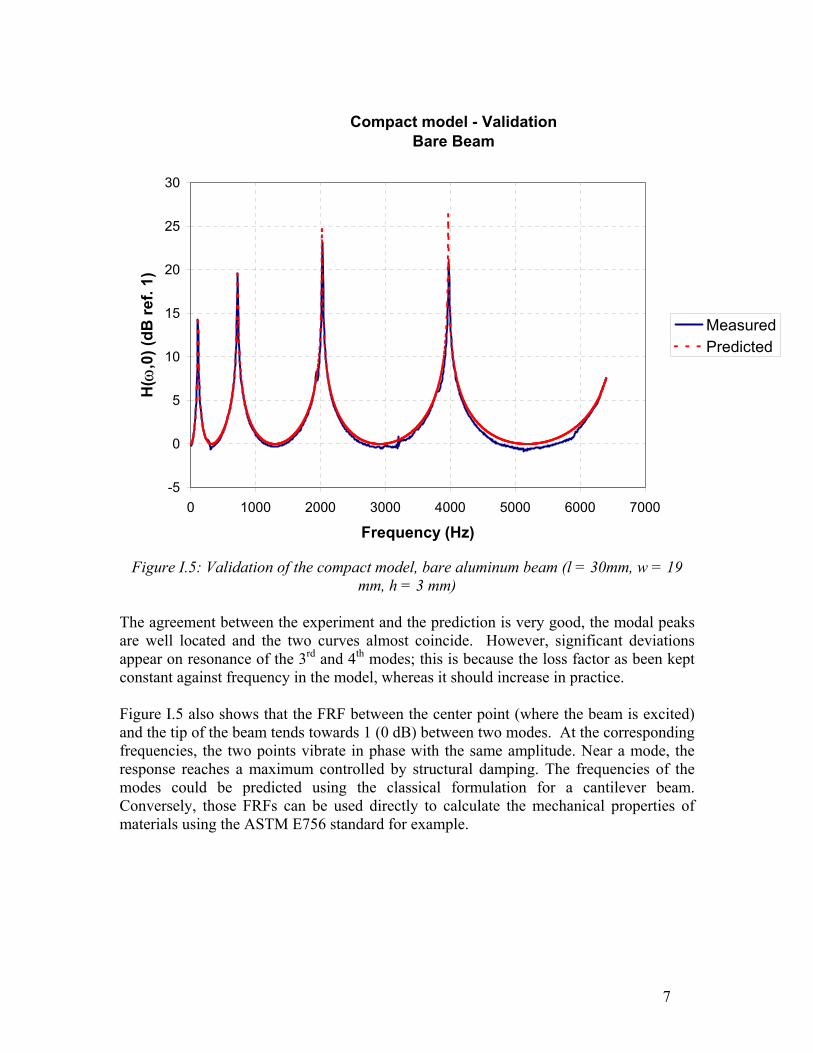
Figure I.5: Validation of the compact model, bare aluminum beam (l = 30mm, w = 19

mm, h = 3 mm) The agreement between the experiment and the prediction is very good, the modal peaks are well located and the two curves almost coincide. However, significant deviations appear on resonance of the 3rd and 4th modes; this is because the loss factor as been kept constant against frequency in the model, whereas it should increase in practice. Figure I.5 also shows that the FRF between the center point (where the beam is excited) and the tip of the beam tends towards 1 (0 dB) between two modes. At the corresponding frequencies, the two points vibrate in phase with the same amplitude. Near a mode, the response reaches a maximum controlled by structural damping. The frequencies of the modes could be predicted using the classical formulation for a cantilever beam. Conversely, those FRFs can be used directly to calculate the mechanical properties of materials using the ASTM E756 standard for example.

7

I.2.3 Inversion of the model

In the following, experimental data of )0,(ωH

)

(free end measurements) are used in conjunction with the above model to extract the properties of foam materials added to a base aluminum beam. The FRF 0,(ωH is measured from two transverse velocity measurements with a laser Doppler vibrometer. It must be noted that the same model is used for both the bare beam and the composite beams. In the second case, the beam is regarded as a homogenous equivalent beam. The extraction procedure follows two steps: • In a first step, an optimization procedure extracts the bending stiffness E~ I )(ω of the

beam under test where E~ is the complex equivalent Young's modulus and I is the equivalent area moment of inertia. This is done for the base beam alone ( bb IE~ )(ω )

and for the composite beam ( E~ I ( )ω ); • The extraction of the mechanical properties of the material (Young's modulus ,

loss factor matE

matη ) is performed in a second step. Extraction of the equivalent bending stiffness The calculation of the rigidity E~ I of the composite beam is performed from experimental FRF on limited frequency bands including only one vibration mode. The order of the mode, dimensions and weight of the beam must be determined before extracting E~ I. Step 1: The software identifies the maximum value of the experimental FRF, and estimates the modal frequency. The structural loss factor is deduced for each mode using the 3 dB bandwidth method. From the values of the modal frequency and loss factor, a

first estimation of the flexural rigidity is performed using the relation µ

κω IEnn

~~ 2= ,

where nω~ is the complex frequency, µ is the lineic mass of the beam and nκ are the modal wavenumbers of the beam, given by

n = 1 κn = 1.875 n = 2 κn = 4.694 n = 3 κn = 7.854 n = 4 κn = 10.995 n > 4 κn = (2n - 1)(π/2)

Step 2: The initial estimate of E~ I is adjusted (real and imaginary parts) iteratively in order to minimize a cost function which is defined as the difference between the experimental and theoretical FRF in the frequency range considered.

Figure I.6 shows an example of the model inversion for the same base aluminum beam as before (length 300 mm, width 19 mm, thickness 3 mm) with a free layer of auto-adhesive damping material (thickness 1 mm); a Young's modulus of 70 Gpa and a constant loss factor of 0.08% have been assumed for the aluminum beam. In this case,

8

the complex composite bending stiffness E~ I has been adjusted in the model at each frequency so that the experimental and theoretical FRF coincide over the whole frequency range. The extracted E~ I therefore varies with the frequency. Note when comparing figures I.5 and I.6 that the addition of a free layer of damping material significantly changes the structural damping of the composite beam, but only slightly affects the resonant frequencies; therefore the FRF has significant sensitivity to the loss factor of the damping material, but much less to the Young's modulus of the damping material. A way to increase the sensitivity of the FRF to the Young's modulus of the tested material is to use a constrained layer configuration; this is detailed in a forthcoming section. In all subsequent experiments, the optimization of E~ I is carried on limited frequency bands around resonance instead of large frequency bands, in order to obtain one value for the loss factor and Young's modulus per mode. One advantage of the proposed method is to calculate the properties of the composite beam using a large number of experimental data points and the exact analytical formulation. In comparison, the ASTM E756 standard uses the values of the modal frequencies (measured at the peaks) and loss factor (measured typically with the 3dB bandwidth method). The modal frequency is equal to the peak frequency as long as the damping is small; in the case of large damping, a correction factor should be applied. Also, the 3dB bandwidth method is a quick , but usually not very accurate way to evaluate the structural loss factor. A curve fitting method is preferable. However, curve-fitting algorithms are based on trial functions, which are not the analytical FRF as proposed in this present work. Therefore, another potential interest of the present approach is to perform optimization on an analytical expression which depicts the real physical problem.

9

Compact model - ValidationComposite Beam

-2

0

2

4

6

8

10

12

14

16

0 1000 2000 3000 4000 5000 6000 7000

Frequency (Hz)

H( ω

,0) (

dB re

f. 1)

MeasuredPredicted

Figure I.6: Example of the model inversion for a composite beam (base beam + free layer of viscoelastic material)

Extraction of the mechanical properties of the material Once bb IE~ )(ω has

been determined for the base beam and E~ I )(ω for the composite beam, the material properties, i.e. Young’s modulus )(ωmatE and loss factor )(ωηmat are extracted. Two cases are considered:

• Extensional damping (Figure I.7)

10

Dampingmaterial

Base beam

bH bH

matHmatH

matH

Single-sided treatment Double-sided treatment

Figure I.7: Extensional damping configurations for material characterization When the damping material is unconstrained (glued on one or two faces of the base beam), the treatment is called extensional damping. As one of the faces of the material is free, the added rigidity is due to bending deformation of the material. It is assumed that the composite beam is subjected to pure bending deformation. The neutral axis of the composite beam is somewhat moved upwards from the position of the neutral axis of the base beam in the case of a single-sided treatment; for symmetry reasons, it remains unchanged for the double-sided treatment. The determination of the material properties is based on the Ross, Ungar and Kerwin3 model for a multi-layer structure. This model allows the flexural rigidity E~ I of a multi-layer beam or plate to be calculated using the properties of the different layers (density, thickness, width, length, Young’s modulus). The following equation gives the equivalent flexural rigidity for a single sided damped beam:

+

×+×++×=22

2222

322 .1

.)1(3.1.~.~

hehe

hheIEIE bb (I.7)

The following equation applies for a double sided damped beam.

bbmatmat IEIEIE .~.~.2.~ += (I.8) with e2: Young’s modulus ratio bmat EE ~/~ h : Thickness ratio Hmat/ Hb 2

E~ b: Young’s modulus of the base beam (Pa) Ib: Area moment of inertia of the base beam with respect to its neutral axis (m4) Hb: Thickness of the base beam (m)

3. A. D. Nashif, D.I.G. Jones, J.P. Henderson, Vibration Damping, John Wiley & Sons, 1985.

11

E~ mat: Young’s modulus of the tested material (Pa) Imat: Area moment of inertia of the tested material with respect to the neutral axis of the composite beam (m4) Hmat: Thickness of the tested material (m) The experiments for extensional damping involved only single sided materials, so that only equation (I.7) was used. The calculation of the complex modulus of the material E~ mat using equation I.7 leads to the solution of an algebraic equation of degree 2 (two complex roots). Only the root with positive real and imaginary parts is selected. The calculation of E~ mat using equation I.8 is trivial. The Young’s modulus and loss factor of the material are determined by identifying the real and imaginary part of E~ mat

using )1(~matmat jEE η=mat +

Shear damping (Figure I.8)

Dampingmaterial

Base beam

matH

bH

bH

Constrained-layer treatment

Constraining layer

Deformation of a beam element

Figure I.8: Shear damping configurations for material characterization When the damping material is sandwiched between the base beam and a rigid constraining layer, the treatment is called shear damping. In this case, the composite beam has a significantly larger flexural rigidity due to the shear deformation of the sandwiched material, which is usually much larger than the bending deformation. Equation I.9 gives the flexural rigidity for a composite beam with a shear damping treatment assuming that the base beam and the constraining layer are identical:

2

2

21.~.1..~.~.2.~

+×+

+=

mat

bmatmat

nmat

bmatmatbb H

HAG

HH

IEIEIEκ

(I.9)

12

with matG~ : Shear modulus of the tested material (Pa) Amat: Cross-sectional area of the tested material (m²)

nκ : modal wavenumbers of a clamped-free beam of length L/2, n = 1 κn = 1.875 n = 2 κn = 4.694 n = 3 κn = 7.854 n = 4 κn = 10.995 n > 4 κn = (2n - 1)(π/2) Imat: Area moment of inertia of the tested material with respect to its neutral axis (m4); note that for shear damping, the definition of Imat is therefore different to extensional damping. The derivation of equation I.9 is detailed in Appendix A. The second term in the right-hand side of equation I.9 is due to the flexural rigidity of the sandwiched material, while the third term is related to shear. For soft materials, the flexural term can usually be neglected for the first modes. However, it is interesting to note that the shear rigidity rapidly decreases as the frequency increases due to the division by whereas the flexural rigidity has a slower frequency dependence. When the flexural term of equation (I.9) is neglected, it simplifies to

2nκ

2

2 1.~.1.~.2.~

+×+=

mat

bmatmat

nbb H

HAGIEIE

κ (I.10)

Therefore, equation (I.10) allows extraction of the complex shear modulus of the material, Gmat

~ . The real-valued shear modulus and loss factor of the material are

determined by identifying the real and imaginary part of G~ mat using )1(~

matmat jG η+= matG . If it is further assumed that the material is homogeneous and

isotropic, )1(2

~~matG

mat

matEυ+

= ; the complex Young’s modulus of the material can therefore

be extracted from equation I.10 provided the Poisson’s ratio of the material is known.

I.2.4 Test specimens Various tests specimens were prepared in order to measure the material properties of foams supplied by DREA. The length of the specimens were 150mm, 270mm or 350mm, depending on the material under test. The base beams were made of aluminum, with a thickness of 1mm or 0.25mm. It was found that for the soft materials considered, thin base beams had to be used in order to obtain a sufficient sensitivity of the measured FRF to the material properties. Also, the material was bonded on the base beam as a free layer (extensional damping), or sandwiched between two identical base aluminum beams

13

(shear damping). Figure I.9 shows an example of a composite beam (the material is constrained between 1mm aluminum beams) attached to the test shaker.

Figure I.9: A test specimen (shear damping configuration) attached to the shaker

I.2.5 Results Tables I.1 to I.4 below detail the measured properties of the foams (Young's modulus or shear modulus, and loss factor).

14

Table I.1 Material characterization using a 1mm base beam and single-sided extensional damping

3 mm neoprene foam 6 mm EVA foam 12 mm EVA foam Beam Beam Beam Length mm Length 270 mm Length 270 mm Width mm Width 25,5 mm Width 25,5 mm Thickness mm Thickness 0,92 mm Thickness 0,93 mm Density kg/m³ Density 2830 kg/m³ Density 2797 kg/m³ Material Material Material Thickness mm Thickness 6,38 mm Thickness 13,5 mm Density kg/m³ Density 74,7 kg/m³ Density 71 kg/m³

Mode Frequency (Hz)

E (Pa) η Mode Frequency (Hz)


E (Pa) η

1 1 41,375 1,74E+06 0,2392 1 44,0 2,32E+06 0,1301 2 2 263 2,05E+06 0,2568 2 276,8 2,28E+06 1,46E-013 3 741 2,22E+06 0,2210 3 761,5 1,87E+06 1,64E-014 4 1450 1,85E+06 0,3084 4 1453,0 1,36E+06 2,23E-015 5 2386 1,25E+06 0,4687 5 2329,0 8,23E+05 3,66E-016 6 3546 1,19E+06 0,2397 6 3386,0 3,78E+05 1,72E+00

6 mm PVC foam 25 mm EPT/SBR foam Beam Beam Length 270 mm Length 350 mm Width 25,6 mm Width 25,4 mm Thickness 0,93 mm Thickness 1,57 mm Density 2784 kg/m³ Density 2739 kg/m³ Material Material Thickness 6,15 mm Thickness 26,8 mm Density 167,2 kg/m³ Density 158 kg/m³

Mode Frequency (Hz)


E (Pa) η

1 37,875 5,35E+05 0,2884 1 41,75 2,86E+06 0,2016 2 2 259 2,66E+06 0,1860 3 3 672 1,76E+06 0,2757 4 4 1324 1,81E+06 0,5739 5 5 6 6

15

Table I.2 Material characterization using a 0.25mm base beam and single-sided extensional damping

3 mm neoprene foam 6 mm EVA foam 12 mm EVA foam Beam Beam Beam Length 150 mm Length mm Length mm Width 25,5 mm Width mm Width mm Thickness 0,28 mm Thickness mm Thickness mm Density 2633 kg/m³ Density kg/m³ Density kg/m³ Matérial Matérial Matérial Thickness 3,22 mm Thickness mm Thickness mm Density 309 kg/m³ Density kg/m³ Density kg/m³

Mode Frequency (Hz)

E (Pa) η Mode Frequency(Hz)


E (Pa) η

1 32,72 3,21E+06 0,0809 1 1 2 205,11 3,21E+06 0,1625 2 2 3 563 2,84E+06 0,2790 3 3 4 1053,28 2,27E+06 0,3875 4 4 5 1523,42 1,47E+06 0,6470 5 5 6 6 6

6 mm PVC foam 25 mm EPT/SBR

foam

Beam Beam Length 150 mm Length mm Width 38,18 mm Width mm Thickness 0,28 mm Thickness mm Density 2614 kg/m³ Density kg/m³ Matérial Matérial Thickness 6,12 mm Thickness mm Density 159 kg/m³ Density kg/m³

Mode Frequency (Hz)

E (Pa) η Mode Frequency(Hz)

E (Pa) η

1 35,89 8,04E+05 0,2396 1 2 225,55 8,78E+05 0,5000 2 3 548,81 5,82E+05 0,6815 3 4 1473,5 3,52E+05 1,4782 4 5 5 6 6

16

Table I.3 Material characterization using a 1mm base beam and shear damping

3 mm neoprene foam 6 mm EVA foam 12 mm EVA foam Beam Beam Beam Length mm Length 270 mm Length 270 mm Width mm Width 25,5 mm Width 25,5 mm Thickness mm Thickness 0,92 mm Thickness 0,93 mm Density kg/m³ Density 2830 kg/m³ Density 2797 kg/m³ Matérial Matérial Matérial Thickness mm Thickness 6,38 mm Thickness 13,5 mm Density kg/m³ Density 74,7 kg/m³ Density 71 kg/m³

Mode Frequency (Hz)

G (Pa) η Mode Frequency(Hz)


G (Pa) η

1 1 100,52 1,13E+06 0,1145 1 118,3 1,05E+06 0,1291 2 2 400,44 1,87E+06 0,1707 2 438,5 1,70E+06 0,1702 3 3 886,3 1,51E+06 0,1878 3 916,8 1,50E+06 0,1685 4 4 1615 1,30E+06 0,2248 4 1613,4 1,36E+06 0,1547 5 5 2572,55 8,89E+05 0,3718 5 2509,5 1,02E+06 0,2450 6 6 3745,07 3,35E+05 1,0677 6 3589,6 3,47E+05 0,5468

6 mm PVC foam 25 mm EPT/SBR foam Beam Beam Length mm Length 270 mm Width mm Width 25,4 mm Thickness mm Thickness 0,93 mm Density kg/m³ Density 2739 kg/m³ Matérial Matérial Thickness mm Thickness 26,8 mm Density kg/m³ Density 158 kg/m³

Mode Frequency (Hz)


G (Pa) η

1 1 524,14 1,86E+07 0,3790 2 2 989,49 1,01E+07 0,2535 3 3 1591,14 8,39E+06 0,1715 4 4 2291,19 7,59E+06 0,1407 5 5 6 6

17

Table I.4 Material characterization using a 0.25mm base beam and shear damping

3 mm neoprene foam 6 mm EVA foam 12 mm EVA foam Beam Beam Beam Length 150 mm Length mm Length mm Width 25,5 mm Width mm Width mm Thickness 0,28 mm Thickness mm Thickness mm Density 2633 kg/m³ Density kg/m³ Density kg/m³ Matérial Matérial Matérial Thickness 3,22 mm Thickness mm Thickness mm Density 309 kg/m³ Density kg/m³ Density kg/m³

Mode Frequency (Hz)


G (Pa) η Mode Frequency (Hz)

G (Pa) η

1 88,36 2,72E+05 0,1537 1 1 2 363,9 5,69E+05 0,3351 2 2 3 765,31 5,29E+05 0,3495 3 3 4 1350,25 5,85E+05 0,3304 4 4 5 1961,5 7,41E+05 0,2793 5 5 6 6 6

6 mm PVC foam 25 mm EPT/SBR foam Beam Beam Length 150 mm Length mm Width 38,18 mm Width mm Thickness 0,28 mm Thickness mm Density 2614 kg/m³ Density kg/m³ Matérial Matérial Thickness 6,12 mm Thickness mm Density 159 kg/m³ Density kg/m³

Mode Frequency (Hz)


G (Pa) η

1 103,83 2,21E+05 0,3669 1 2 452,45 5,77E+05 0,6742 2 3 928,12 7,36E+05 0,4660 3 4 4 5 5 6 6

18

Figures I.10 and I.11 show the frequency dependence for the Young's modulus and loss factor of the various materials and compares the values obtained with extensional (single-sided) and shear (constrained layer) techniques (the shear modulus G measured with the constrained layer technique was used to derive a Young's modulus E according to the isotropic relation GE )1(2 ν+= ; a value of 35.0=ν was assumed for the Poisson coefficient). Both techniques give values of the Young's modulus in the Mpa range for the various materials investigated, although significant differences are observed between extensional and shear measurements of E (in general, the shear technique gives larger values of E than the extensional measurement). The very large differences found in the case of the 25mm EPT/SBR foam may be due to the non-respect of the thin beam hypothesis in this case. As far as loss factor is concerned, we note that extensional and shear measurements are in fairly good agreement at the low frequency end of the spectrum. As a general comment, the extensional technique was found to be much less sensitive than the shear technique for the materials investigated.

Young's modulus - 3mm neoprene

0,00E+005,00E+051,00E+061,50E+062,00E+062,50E+063,00E+063,50E+06

0 500 1000 1500 2000 2500

Frequency (Hz)

Youn

g's

mod

. (Pa

)

ShearExtensional

Loss factor - 3mm neoprene

0,00000,10000,20000,30000,40000,50000,60000,7000

0 500 1000 1500 2000 2500

Frequency (Hz)

Loss

fact

or

ShearExtensional

Young's modulus - 6mm PVC

0,00E+00

5,00E+05

1,00E+06

1,50E+06

2,00E+06

2,50E+06

0 500 1000 1500 2000

Frequency (Hz)

Youn

g's

mod

. (Pa

)

ShearExtensional

Loss factor - 6mm PVC

0,00000,20000,40000,60000,80001,00001,20001,40001,6000

0 500 1000 1500 2000

Frequency (Hz)

Loss

fact

or

ShearExtensional

Figure I.10: Comparison of Young's modulus and loss factor frequency dependence obtained with extensional (single-sided) and shear (constrained layer) techniques: 3mm neoprene and 6 mm PVC

19

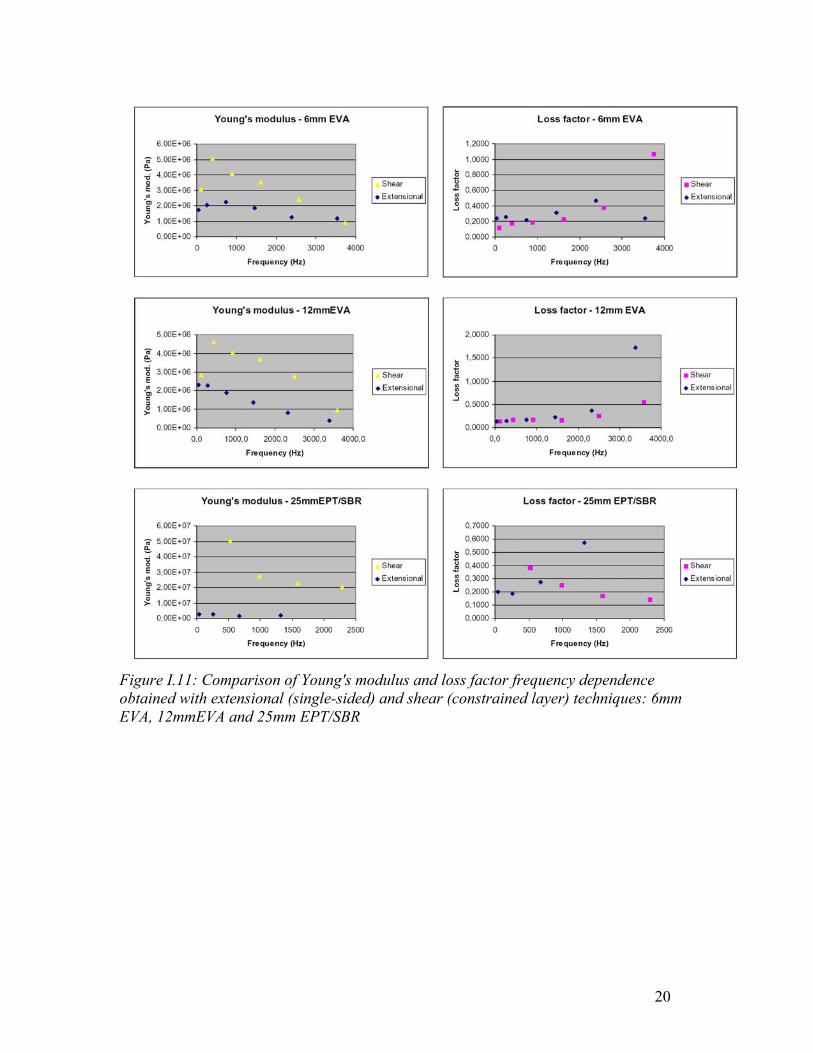
Figure I.11: Comparison of Young's modulus and loss factor frequency dependence obtained with extensional (single-sided) and shear (constrained layer) techniques: 6mm EVA, 12mmEVA and 25mm EPT/SBR

20

Table I.5 shows the experimental characterisation results obtained from different labs (ref, J.P. Szabo, email of 23/02/01). As a general observation, the modulus values obtained from the Oberst beam technique are larger than those obtained from compression techniques. Since the Oberst beam technique essentially measure the modulus in the in-plane direction of the foam, and compression techniques measure the modulus in the transverse direction, a possible explanation (apart from strictly experimental problems) is the anisotropy of the material. Table I.5 Dilatational modulus of tested materials obtained by different laboratories

Dilatational Modulus (L) in MPa

GAUS GAUS GIL TNO DREA DREA Frequency Range 0-2kHz 0-2kHz 100- 900 Hz 0 - 200 Hz 0.1 Hz 0.1 - 5 Hz Method Oberst Oberst Shaker Shaker DMTA Instron Mode Extensional Shear Compression Compression Compression

and Shear Compression

Size of Sample (mm) 150-350 x 25 150-270 x 25 150 diameter 130 diameter ~ 30 diameter 300 diameter

3 mm neoprene foam 2,4-4,8 0,8-3,2 0,68 0,4712 mm EVA foam 0,8-3,2 1,6-8 3,00 1,246 mm EVA foam 1,6-3,2 1,6-8 3,00 1,246 mm PVC foam 0,8-1,6 0,8-3,2 0,20 0,1625 mm EPT/SBR foam 3,2-4,8 32-80 1,00 0.3 - 0.5

21

VIBRATION MEASUREMENTS AND COMPARISONS WITH VIBRO

2.1 Experimental set-up

The tested plate and the tested coating are installed in the water tank (Figure II.2). The excitation is provided by a shaker on the air side of the plate, driven by the control computer generator (LMS software) and a power amplifier. The injected force and the acceleration at the driving point on the air side are measured with an impedance head. The vibration measurement both on the water side of the plate and on the air side is made using a laser vibrometer connected to a system of mirrors (Figure II.1) in order to steer the laser beam on the meshing points. The laser beam is pointed between each acquisition on the following meshing point by this mean.

Mirror with step-to-step motors,allowing to move it from a control box.Laser Vibrometer

Figure II.1 Close-up of laser vibrometer and mirror

22

Control computer (LMS) 4. Power amplifier

3. Shaker

5. Charge amplifier

1. Laser vibrometer

Water tank

Plate & coating

2.Impedance head

Figure II.2 Experimental set-up

The measurement instrumentation is as follows: 1. Laser Vibrometer Polytec OFV 302 2. Impedance head ICP mod. PCB # 288 D01 3. Shaker Brüel and Kjaer 4810 4. Power amplifier Brüel and Kjaer type 2706 5. Conditioner ICP PCB model 482 A17 The following pictures give an overview of the experimental set-up.

23

2

3

Figure II.3 View of the excitation side of the water tank

LMS

1

4

5

Figure II.4 View of the acquisition/measurement side of the water tank

24

Water tank and frame The tank is 0.55 x 0.42 x 0.64 m (contenance about 150 L) and is made with PVC. The side opposite to the plate is made of transparent Plexiglas to allow appropriate transmission of the laser beam through it. It is filled with distilled water in order to minimize the air content of the water, and an algaecide (copper sulfate) is added to keep the water clear. On the plate side, the tank is open and a steel frame is inserted to allow the fixation of the plate as described below. Plate & coating installation and boundary conditions • The plate dimensions are 0.5 x 0.35 m; • The plate (plus coating) to be tested is inserted as one side of the tank; • The plate is mounted on quasi simply supported boundary conditions; in a first

instance, the simply supported conditions were realized using thin blades perpendicular to the plate and bonded to the plate edges. These thin aluminum blades are fixed inside a steel frame by the mean of beams and screws to ensure minimum leakage from the tank, as shown in Figure II.5:

1 cm

Water side Air side

Plate to be tested

Aluminium blades Steel frame

Beam and screws

Figure II.5 Experimental boundary conditions for the 2mm steel plate This mounting procedure worked well for a thin (2mm) steel plate, and was therefore implemented in the experiments involving the 2mm plate. However, for the thicker plate (9.5mm), it was observed that a significant amount of transverse vibration was transmitted to the frame and tank through the supports; also, the small aluminum blades were not rigid enough to ensure a zero transverse displacement at the edges of the plate. As a consequence, the simply-supported boundary condition was not respected for a thick plate. Finally, it was found that in this case, the large vibration transmission to the tank structure resulted in a poor experimental coherence between the applied force to the plate and the plate response.

25

Consequently, an alternative fixture was used for thick plates. Small aluminum blades coplanar to the plate are inserted between the plate and frame (Figure II.6).

1 cm

Steel frame

Beam and screws

Aluminium blades

Plate to be tested

Air side Water side

Figure II.6 Experimental boundary conditions for the 9.5mm steel plate

This modification allows to minimize vibration transmission to the tank structure, as the aluminum blades have a low stiffness. However, the boundary conditions are no longer simply supported, as this configuration allows a displacement at the edges of the plate. It is believed however, that boundary conditions of the plate have a moderate impact on the amount of vibration reduction provided by the decoupling coating. In order to provide sufficient space for the aluminum blades, the size of the 9.5mm plate was slightly reduced (0.48x0.33 m), as compared to the 2mm plate. The results of Figure II.7 show the vibration transmission between the 9.5mm test plate and the tank structure for the two boundary conditions of Figures II.5 and II.6; the results compare the mean square velocity measured on the plate and on the supporting steel frame for the two fixation systems. The new fixation system provides better vibration isolation of the frame and tank structure.

26

Figure II.7 Comparison of the vibration transmission between the test plate and supporting frame for the two types of plate fixation.

In both configurations, a silicon seal is added at the edges and corners of the plate and aluminum blades to prevent water leakage. Also, • The tested coating is bonded to the wet side of the tested plate. Note that even though

the 3 mm neoprene foam was pre-bonded, an additional layer of glue was necessary in order to provide sufficient bonding in water;

• A reflective film is added on both the water side and the air side to ensure proper reflection to the laser beam.

• The steel plate and frame are prevented from rusting by the use of a lacquer layer, in order to keep a clear transparent water for the laser measurement.

2.2 Acquisition and analysis

2.2.1 Acquisition

There are three channels of acquisition :

- Channel 1 : Force (reference channel) - Channel 2 : Acceleration at the driving point - Channel 3 : Velocity from the laser vibrometer

From impedance head through ICP conditioner

27

These channels are connected to the control computer through the LMS interface. The laser is manually pointed on a new point between each acquisition. The LMS station is used for the acquisition. It calculates power auto-spectrum for each channel, and Frequency Response Functions (FRF) and coherence between channel 1 and 2, and between channel 1 and 3. The FRF are evaluated with the H1 estimator, which means that in the case of transverse velocity measurement,

><><

=**

ffvfFRF (II.1)

where is the power cross-spectrum between the measured velocity and driving force, is the power auto-spectrum of the driving force.

>< *vf>< *ff

The acquisition parameters are as follows: • Frequency range : LMS only allows to choose the upper frequency and the number

of spectral lines (among 2n values). As the exploitable range of measure is 78.5% of the acquisition range, the upper limit of acquisition should be at least 5120 Hz in order to cover a 0-4000Hz frequency range. However, if the resolution is different to 1 Hz, it is not possible to easily set up the frequency range (this is a problem when the acquisition is done in several bands, see below). To meet those two requirements, the upper frequency was set equal to 8192 Hz, with a resolution of 1 Hz (first 2n value above 5120 Hz). However, this was not the case for all measurement; the parameters chosen were:

- 2mm plate: 0-4096 Hz, 1Hz resolution - 2mm plate with coating: 0-5120 Hz, 1.25Hz resolution - 9.5mm plate without/with coating: 0–8192 Hz, 1Hz resolution. • Averaging: 25 averages per measurement point; • Excitation signal: The excitation is a random noise on the full or partial frequency

range, with a burst length of 50% of the measurement duration. The acquisition is triggered on the source.

• Acquisition in multiples band: If the measurement shows a good coherence on all

the frequency range, the acquisition can be made in only one band. However, as the magnitude of the driving force decreases when frequency increases, it may be necessary to perform the acquisition in multiple successive bands. The figure II.8 below shows that acquisition in multiple bands may have a large impact on the signal/noise ratio.

28

Figure II.8 Single-band vs. multiple-band acquisition.

2.2.2 Analysis

LMS produces at each measurement point, 5 data files of 4096 points (containing real and imaginary part) corresponding to the following results:

- power auto-spectrum of the force - acceleration/force coherence - velocity/force coherence - acceleration/force FRF - velocity/force FRF.

LMS data are exported as universal files. Useful information is extracted and processed with MATLAB, and results are saved as Matlab files. The results are therefore available in both .UFF and .mat format. The useful experimental indicators are:

• Mean square velocity ∫∫>=s

dSvS

v ²121² <

29

In discrete form:

∑ ∑= =

>=<m

i

n

jijij Sv

Sv

1 1

2121² (II.2)

where v is the complex velocity measured at point ij and is the elemental plate area.

Assuming the meshing is regular, ij ijS

cteSS eij == , and eS kS= , with the total number of meshing points. Hence:

mnN =

)(211

21²

2

1 1

2ij

m

i

n

jij vmeanv

Nv ∑ ∑

= ==>=< (II.3)

For comparisons with the theory, the mean square velocity of the plate is divided by the squared magnitude of the driving force,

)/(21/1

21/² 22

1 1

222 fvmeanfvN

fv ijm

i

n

jij∑ ∑

= ===>< , (II.4)

that is,

)),((21/² 2 jiFRFmeanfv =>< (II.5)

where is the force-velocity FRF at point ij. In dB, ),( jiFRF

210 /²log10² fvv ><>< 2/ f dB =

• The mean square velocity ratio for a coated plate is defined as ratio of the mean

square velocity measured on the air-side and on the water-side:

sidewater

sideair

fv

fvVR

−

−

><

><= 2

2

10/²

/²log10 ; (II.6)

• The insertion loss is defined as the ratio of the mean square velocity of the bare plate

to the mean square velocity of the coated plate (measured on the water-side):

sidewaterplatecoated

platebare

vv

IL−−

−

><

><=

,10 ²

²log10 (II.7)

30

2.2.3 Preliminary tests Linearity The linearity of the experiment was verified by checking the invariance of the FRF for different levels of excitation. Coherence Coherence is also a good indicator of the quality of a measurement. The coherence between the driving force and the plate velocity at an arbitrary position (air side and water side) is shown on Figure II.9. The coherence starts to drop in higher frequency, especially when measured on the water side of the plate.

Figure II.9 Coherence measurement between the driving force and the plate velocity.

31

Laser vibrometry through water The surface velocity measurement on the coating using a laser vibrometer implies that the laser beam crosses three different media : air, the plexiglas side of the tank and water. We have checked that the loss of the reflected signal in this case did not alter the surface velocity measurement, by comparing the mean square

Figure II.10 Mean square velocity of a steel plate measured with the laser vibrometer on the air side and on the water side.

velocity of an uncoated plate measured on the air side and on the water side (Figure II.10). The agreement is generally good, which validates the laser measurement in water.

32

2.2.4 Characteristics of test plates and of measurements

Dimensions (m)

Thickness (mm)

Density (kg/m³)

Young'sModulus

(Pa)

Loss factor

Poisson coefficient

2 mm plate 0.5 x 0.35 1.82 7850 11102× 0.005 0.3 Plates

9.5 mm plate 0.48 x 0.33 10.00 7850 11102× 0.005 0.3

3 mm neoprene

foam 0.5 x 0.35 3.22 309 Frequency

dependant Frequency dependant 0.45

6 mm EVA foam 0.5 x 0.35 6.38 74.7 Frequency


Coating materials

25 mm EPT/SBR

foam 0.48 x 0.33 26.8 158 Frequency


The frequency dependant characteristics of decoupling materials (Young's modulus and loss factor) are detailed in section I.2.5

Driving point : the driving point was chosen so that as many plate modes as possible are excited. The driving point was located at the position (0.1625m,0.1625m) from a corner of the plate. Meshing : The initial criterion to accurately measure the mean square velocity of the plate was 4 measurement points per wavelength at the maximum frequency considered (4kHz). This criterion resulted in 280 points for the 2mm plate and 96 points for the 9.5mm plate. However, since the derivation of mean square velocity does not require phase information, the requirement for the number of data points can be significantly relaxed (See Figure II.11 for tests on the 2mm plate immersed in water). Also, it was verified that measurement points on the air side of the plate can be taken to cover only a limited area of the plate (half the plate instead of the full plate, see Figure II.11). In practice, laser measurements on the air side cannot be performed on the full plate, because of the volume occupied by the shaker and its support.

33

Figure II.11 Mean square velocity measurements on the 2mm steel plate with various meshes.

The final configuration for the excitation and measurement on the plate is shown on Figure II.12

0

Water side measurement surface

Air side measurement

Excitation point 0.1625 x 0.1625 m

x y

z

Figure II.12 Measurement configuration on the test plate

34

The useful measurement parameters are listed in the following table.

Meshing LMS parameters

Test plate Number of points

Fraction of the plate

measured

x-step y-step (cm)

Number of acquisition bands and frequency separation

Frequency range (Hz)

Frequencyresolution

Air side 140 Half 2.5 2.5 1 0 – 4096 1 Hz 2 mm steel

plate Water side 280 Full 2.5

2.5 2

Fs=1600 Hz 0 – 4096 1 Hz

Air side 70 Half 2.5 5 1 0 – 5120 1.25 Hz2 mm steel

plate + 6 mm EVA

foam Water side 70 Full 5 5 1 0 – 5120 1.25 Hz

Air side 70 Half 2.5 5 1 0 – 5120 1.25 Hz2 mm + 3

mm neoprene

foam Water side 70 Full 5 5 1 0 – 5120 1.25 Hz

Air side 30 Half 4.8 5.5

2 Fs=2000 Hz 0 – 8192 1 Hz 9.5 mm steel

plate Water side

Air side 30 Half 4.8 5.5

2 Fs=2000 Hz 0 – 8192 1 Hz 9.5 mm steel

plate + 25 mm

EPT/SBR foam

Water side 60 Full 4.8 5.5 2

Fs=2000 Hz 0 – 8192 1 Hz

35

2.3 Comparisons with VIBRO predictions

2.3.1 VIBRO parameters The input parameters of WinVibro are : Frequency range : • The frequency range used in each case is 10 – 4000 Hz; • The frequency resolution used is generally 1 Hz but can be adjusted according to

accuracy needs; • Frequency interpolation for Gauss points integration (fluid-structure coupling): 10

Hz; • The modal order and the number of Gauss points are adjusted in each case to meet

both reasonable requirements of accuracy and computation time. Characteristics of fluid media :

Medium Density (kg/m³)

Sound velocity (m/s)

Air 1.29 340

Water 1000 1460 Characteristics of plate and coating : The plate and coating properties to be input in the model have been discussed in the previous sections. Note that when the locally reacting model is used in VIBRO, the Young's modulus of the material is replaced by the plate modulus calculated from the relation µλ 2+=L , where µλ, are the Lamé of the material. Excitation : The excitation on VIBRO is a point force of amplitude 1N at the location detailed in section II.2.4.

2.3.2 Steel plate in air As an initial verification, the response of a 2mm steel plate was measured with no water in the tank, in order to make sure that the dynamics of the plate, tank structure and boundary conditions conform to the model, and that the experimental procedure is reliable. The experiment was conducted with 140 measurement points covering half the area of the plate. VIBRO has been run with following parameters :

36

Frequency range

Modal order and number of gauss interpolation points

Resolution(Hz)

0 – 1000 Hz 7 1 1000 – 4000 Hz 10 2

The results are presented on figure II.13:

0 500 1000 1500 2000 2500 3000-80

-70

-60

-50

-40

-30

-20

-10

frequency (Hz)

<v²>

(dB)

comparison between <v²> experimental and VIBRO calculation of <v²>

Figure II.13 Mean square velocity of the bare 2mm steel plate in air, VIBRO-experiment comparison.

The experimental curve fits very well with the VIBRO curve. The modal behaviour predicted by VIBRO conforms to the measurement. Note that the amount of damping present in the system in the absence of any coating is very small.

2.3.3 Steel plate in water 2 mm plate Input parameters of VIBRO are as follows:

37

Frequency range

Modal order

Number of Gauss interpolation points

Resolution(Hz)

10 – 700 Hz 7 7 0.5 700 – 1800 Hz 10 10 1 1800 – 4000 Hz 12 12 1

Figure II.14 shows the VIBRO-experiment comparison. The agreement is satisfactory, as VIBRO is able to capture the complex modal behaviour of the plate coupled to the fluid, especially in low frequency. The free field assumption in VIBRO does not seem to considerably affect the plate response in this case. Note by comparing Figures II.13 and II.14 that the position of the modal peaks is changed by the fluid; also the system is still very reverberant, which implies that the radiation damping is small in this case (the critical frequency of a 2mm steel plate in water is of the order of 100kHz).

9.5 mm plate Input parameters of VIBRO :

Frequency range

Modal order


Resolution(Hz)

10 – 4000 Hz 9 9 1

When immersed in water, the thick plate has a highly damped measured response (Figure II.15). It was verified that this damping is not related to the boundary conditions of the thick plate: the response was also measured in the absence of water, and showed well defined modes in this case. Therefore, it is suspected that the increased damping in water is related to a strong coupling with the fluid (a 9.5mm steel plate in water has a critical frequency of the order of 20kHz, and is therefore a much more efficient radiator than a 2mm plate in the 0-4kHz frequency range). The VIBRO predictions in this case show some deviations with the experimental data, although a strong radiation damping is also predicted. Note that in this case, the experimental boundary conditions are probably less rigid than simply supported conditions, which may explain the important mode shifts in low frequency.

38

2.3.4 2mm steel plate with 3mm neoprene foam

In this configuration as well as in other plate / material configurations, the following data are reported:

• mean square velocity on air side 210

2 /²log10/² fvfv airsidedBairside ><=>< • mean square velocity on the material surface

210

2 /²log10/² fvfv watersidedBwaterside ><=><

• mean square velocity ratio sidewater

sideair

fv

fv

−

−

><

><= 2

2

10/²

/²log10VR

• insertion loss sidewaterplatecoated

platebare

vv

IL−−

−

><

><=

,10 ²

²log10

Comparisons of the experimental results with VIBRO3D (3D elasticity model of the decoupling material) as well as VIBRO1D (locally reacting model) are presented in all cases. In addition, the insertion loss data are compared with the simple model of House, which is briefly recalled below. In some cases, both narrow band and 1/3 octabe band results are shown. For all comparisons between experiments and theory, the following legend is used : Experimental data Model Recall of theoretical considerations The model of House predicts the insertion loss from the calculation of the sound transmission loss of a multilayer system below:

( ) ( ) ( ) ( )

( ) ( ) ( ) ( )

++

++

+−

+

==

4

2

2

13322

4

3

3

13322

42

31

3

23322

4

13322

104

cossinsincos

sinsin1coscoslog20

zz

zz

lklkjzz

zz

lklkj

zzzz

zz

lklkzz

lklk

WW

TLtrans

inc

where iii cz ρ= is the acoustic impedance of the medium i, i=1..4 (respectively air, steel

plate, coating and water); iρ is the density, is the acoustic velocity,ici

i ck ω

= is the

acoustic wavenumber; are the thickness of the plate and coating, respectively. In the model of House, the insertion loss is defined by:

32 , ll

40

344310log10 TLTLWWW

WIL transtrans

with

without −=−==

where is obtained by taking 3TL 03 =l . The above definition of IL is not strictly equivalent to the measured IL, which is rather defined in terms of surface velocity data. The model of House predicts a mass-spring mode of the system, at the frequency approximately given by

333322

3 2 where,21 µλ

ρπ+== L

llL

Fr is the plate modulus of the coating material.

Coating modes are also singular frequencies of the system; the natural frequency of coating modes is given by:

[ ∞∈∀= ;1,2 3

nl

ncf Ln [ , with

3

33 2ρ

µλ +=Lc

Coating modes are associated with a large velocity response at the surface of the material, and therefore a drop in the decoupling efficiency of the material. The above formula shows that increases with the Young's modulus of the material and is inversely proportional to the material thickness. The following table lists the first coating mode of the tested materials; it appears that the coating modes occur at higher frequencies than investigated in the experiments.

nf

3 mm neoprene foam

30 823Hz

6 mm EVA foam 23 295 Hz 25 mm EPT/SBR foam

4 888 Hz

The input parameters of VIBRO 1D and VIBRO 3D for the 2 mm plate + 3 mm neoprene foam are:

Frequency range

Modal order


Resolution (Hz)

10 – 4000 Hz 9 9 1

41

The 3 mm neoprene foam is a material with a large loss factor in high frequency; the experimental data show indeed a transition from highly modal response in low frequency to a highly damped, smooth response in high frequency. The VIBRO3D results should be considered with caution since the code is not able to predict any low frequency mode. It was found that in this case VIBRO3D largely overestimates the resonant frequencies of the system. The modes of the system in this case are shifted to higher frequency and are smoothed out because of the large loss factor of the material. This problem was previously observed in situations where the decoupling material has a large enough rigidity; it is suspected that the origin of the problem is numerical, although it has not been precisely identified yet. However, VIBRO3D gives the correct tendencies for responses on both the air and material side, although it tends to overestimate the vibration attenuation provided by the decoupling material. In this case the simplified VIBRO1D model seems to better fit; it predicts modes at low frequency, but with an overestimated amplitude, because of massless assumption which provides less damping. The tendencies predicted are also closer to experimental data. On the airside, the response of the plate shows a dip between 700 and 1000 Hz, that neither VIBRO1D nor VIBRO3D have predicted. This is particularly visible on the mean square velocity ratio (Figure II.18), which shows a frequency range below 1.5kHz where the velocity ratio is negative, whereas predictions show an almost linear progression of the ratio. It was verified that this frequency does not correspond to either the mass-spring mode or a coating mode (which appears on the model of House in the insertion loss at a higher frequency). The appendix C shows additional experimental results obtained with two different water volumes in the water tank (in fact, the z-dimension of the tank, in the direction perpendicular to the plate was modified so that the water volume was half that of the original tank). These results show that the dip on the airside response is not strongly modified by the change of water volume; therefore, this dip is apparently not related to the finite acoustic volume in the tank. The origin of this singularity in the airside response remains unclear; it should be noted here that the updated model of DeJong, however, seems to adequately predict this phenomenon (see next section). In terms of the velocity ratio, VIBRO1D and VIBRO3D are close and, with the exception of the 0-1.5kHz range, fit quite well with experimental data. The amount of vibration reduction reaches 10 dB at 4000 Hz.

The insertion loss is presented on Figure II.19 in third octave band. Experimental data fall between the VIBRO1D and VIBRO3D predictions in low frequencies, and show the same tendencies in higher frequency. The vibration attenuation provided by the material, compared to the bare plate, is around 20 dB at 4000 Hz. It is to be noted that the model of House significantly deviates from experimental data in this case. Additional theory-experiment comparisons for the 3 coating materials investigated in this work (neoprene, EVA and EPT foams) are presented in Appendix B. In these comparisons, the theoretical predictions are based on properties of the decoupling

42

material derived from either extensional or shear damping measurements reported in Tables I.1-4, or material data measured by DREA, GIL or TNO. These comparisons show that, in general, our material data derived from shear damping measurement better match the experimental results.

43

Figure II.16 Mean square velocity on airside of the 2mm steel plate + 3mm neoprene foam, VIBRO-experiment comparison.

44

Figure II.17 Mean square velocity on waterside of the 2mm steel plate + 3mm neoprene foam, VIBRO-experiment comparison.

45

0 500 1000 1500 2000 2500 3000 3500 4000-25

-20

-15

-10

-5

0

5

10

15

freq (Hz)

Mea

n sq

. vel

. Rat

io V

R (d

B)VIBRO 1D

VIBRO 3D

Experimental data

Figure II.18 Mean square velocity ratio sidewater

sideair

fv

fv

−

−

><

><= 2

2

10/²

/²log10VR ,

2mm steel plate + 3mm neoprene foam, VIBRO-experiment comparison.

46

Figure II.19 Insertion loss sidewaterplatecoated

platebare

vv

IL−−

−

><

><=

,10 ²

²log10 , 2mm steel plate +

3mm neoprene foam, VIBRO-experiment comparison.

3mm neoprene foam

VIBRO 3D, third octave Experimental data, third octave Vibro 1D, third octave House

Inse

rtion

loss

IL (d

B)

40

30

20

10

0

-10

-20

400035003000 25002000freq (Hz)

15001000500 0-30

47

Comparison with the model of DeJong DeJong has developed a one-dimensional model to predict the decoupling performance of a compliant coating on an infinite plate4. This model is an "updated" version of the original one-dimensional model of House, that accounts for dissipation in the coating and radiation mechanisms of finite plates. Figure II.20 shows the comparison between the measured mean square velocity ratio

sidewater

sideair

fv

fvVR

−

−

><

><= 2

2

10/²

/²log10 and the values predicted by the models of House

and of DeJong, for the 2mm steel plate + 3mm neoprene foam. In figure II.20 (a), the complex Young's modulus of the coating has been deduced from the extensional damping measurements (Young's modulus E, loss factorη ) of Table I.2 for the 3mm neoprene foam. In figure II.20 (b), the complex Young's modulus of the coating has been deduced from the shear damping measurements (shear modulus G, loss factorη ) of Table I.4 for the 3mm neoprene foam. It appears from Figure II.20 that the model of Dejong is much more in agreement with the experiments than the model of House. Additionally, the model of DeJong predicts the VR dips which is observed in the experiment. Figure II.21 shows the comparison between the measured acoustic insertion loss IL and the values predicted by the models of House and of DeJong, for the 2mm steel plate + 3mm neoprene foam. In this case, the "measured" acoustic insertion loss is defined (in accordance with the calculated values) as the ratio of the radiated sound power with and without the coating; the radiated sound power was therefore obtained from the experimental surface velocity distributions assuming free-field radiation conditions. Both models satisfactorily agree with the acoustic insertion loss derived from the vibration measurements. 4 The model is detailed in a 11-page document authored by Dr. DeJong and provided to us by Dr. Szabo.

48

House

DeJong

(a) Coating properties derived from extensional damping measurement

House

DeJong

(b) Coating properties derived from shear damping measurement


sideair

fv

fv

−

−

><

><= 2

2

10/²

/²log10VR ,

2mm steel plate + 3mm neoprene foam, comparison between experiments and the models of House and Dejong.

49

House

DeJong


House

DeJong


Figure II.21 Acoustic insertion loss, 2mm steel plate + 3mm neoprene foam, comparison between experiments and the models of House and Dejong.

50

2.3.5 2mm steel plate with 6mm EVA foam

The input parameters of VIBRO1D and VIBRO3D are:

Frequency range

Modal order


Resolution (Hz)

10 – 4000 Hz 10 10 1 The 6 mm EVA foam has a modulus similar to the 3 mm neoprene foam, but a much lower density. As for the 3mm neoprene foam, it is suspected that VIBRO3D results are not reliable in this case. VIBRO1D results are generally in better agreement with the experiment. The same dip in the air side response is noticeable between 700 and 1000 Hz, producing an important difference between experimental velocity ratio and predictions of VIBRO (Figure II.22). Again, above 2000 Hz, predictions agree quite well with the experimental data (Figure II.24); VIBRO1D slightly overestimates the vibration reduction. The amount of vibration reduction reaches 10 dB at 4000 Hz. Insertion loss results (Figures II.25, II.26) also show a good agreement between experimental data and VIBRO1D, especially in high frequency. Again, the model of House significantly deviates from the experiments. Figures II.27, II.28 show comparison between experimental data and the models of House and DeJong in terms of the mean square velocity ratio (Figure II.27) and acoustic insertion loss (Figure II.28) (in the latter case, the free-field sound power was calculated from surface velocity distributions as explained in II.3.4). Again the model of DeJong adequately describes both the vibration and radiation phenomena. It is worthwhile noticing that coating material properties derived from shear damping measurements seem to better fit with the experimental data (Figure II.27-b).

51

Figure II.22 Mean square velocity on airside of the 2mm steel plate + 6mm EVA foam, VIBRO-experiment comparison.

52

Figure II.23 Mean square velocity on waterside of the 2mm steel plate + 6mm EVA foam, VIBRO-experiment comparison

53

Figure II.19 Insertion loss, 2mm steel plate + 6mm EVA foam, VIBRO-experiment comparison.

Inse

rtion

Los

s (d

B)

6mm EVA foam

Experimental data (third octave) Vibro 3D (third octave) House

40

30

20

10

0

-10

-20

0-30

500 1000 1500 2000 freq (Hz)

2500 3000 3500 4000


platebare

vv

IL−−

−

><

><=

,10 ²


6mm EVA foam, VIBRO3D-experiment comparison.

55

6mm EVA foam

Experimental data (third octave) House Vibro 1D (third octave)

40

30

20

10

0

-10

-20

0-30

Inse

rtion

Los

s (d

B)

500 1000 1500 2000

freq (Hz) 2500 3000 3500 4000


platebare

vv

IL−−

−

><

><=

,10 ²


6mm EVA foam, VIBRO1D-experiment comparison.

56

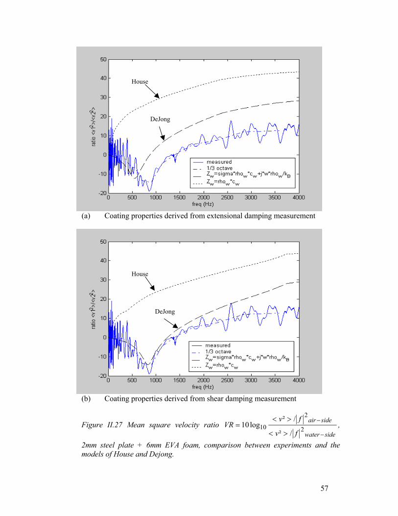
House


House

DeJong

DeJong



sideair

fv

fv

−

−

><

><= 2

2

10/²

/²log10VR ,

2mm steel plate + 6mm EVA foam, comparison between experiments and the models of House and Dejong.

57

House

DeJong


House

DeJong


Figure II.28 Acoustic insertion loss, 2mm steel plate + 6mm EVA foam, comparison between experiments and the models of House and Dejong.

58

2.3.6 9.5mm steel plate with 25 mm EPT/SBR foam

Input parameters of VIBRO1D and VIBRO3D:

Frequency range

Modal order


Resolution

10 – 4000 Hz 7 7 1 In this case, the plate and the coating material are far thicker that in the two previous cases. It results in a lower modal density and a lower response level, too. As already pointed, the experimental boundary conditions in this case deviate from simply supported, which makes the comparisons with the theory more difficult. The experimental response on the material side does not decrease progressively when frequency increases but rather presents a drop around 1000 Hz, and then keeps a relatively constant level (Figure II.30). In contrast, VIBRO predicts a monotonic decrease with the frequency, which results in a large over-estimation of the vibration reduction. VIBRO3D overestimates the velocity ratio by 10 to 15 dB (Figure II.31), and the insertion loss by 10 dB (Figures II.32, II.33), whereas VIBRO1D overestimates the velocity ratio by 15 to 20 dB and the insertion loss by 20 dB. Figures II.34, II.35 present comparisons with the model of DeJong. As a general trend, theoretical results based on shear damping characterisation of the material seem to better agree with the experiments.

59

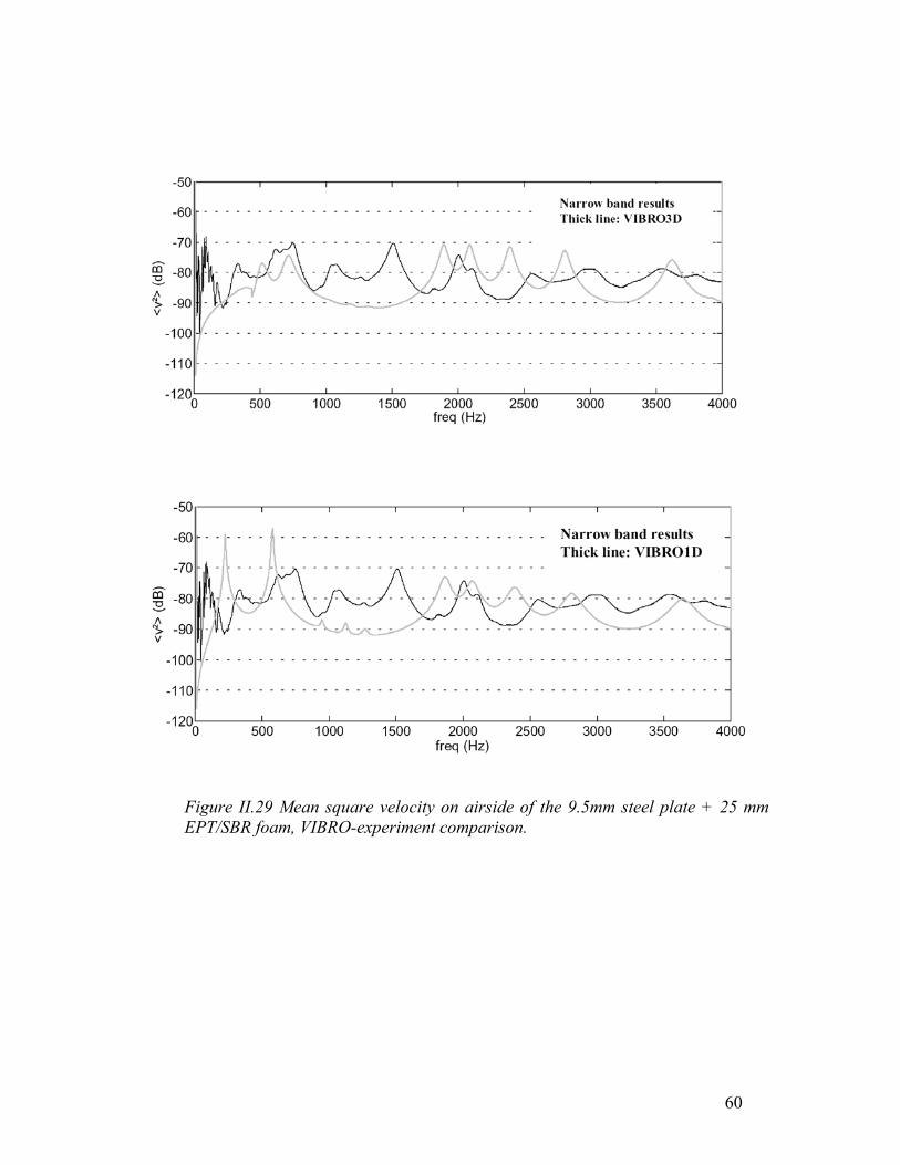
Figure II.29 Mean square velocity on airside of the 9.5mm steel plate + 25 mm EPT/SBR foam, VIBRO-experiment comparison.

60

Figure II.30 Mean square velocity on waterside of the 9.5mm steel plate + 25 mm EPT/SBR foam, VIBRO-experiment comparison.

61

-10

0 500 1000 1500 2000 2500 3000 3500 4000

0

10

20

30

40

freq (Hz)

Mea

n sq

. vel

. Rat

io V

R (d

B)

VIBRO 1D

VIBRO 3D

Experimental data


sideair

fv

fv

−

−

><

><= 2

2

10/²

/²log10VR ,

9.5mm steel plate + 25mm EPT/SBR foam, VIBRO-experiment comparison.

62

25 mm EPT/SBR

Experimental data VIBRO 3D Experimental data, third VIBRO 3D, third octave House

40

30

20

0

0

1

Inse

rt. lo

ss (d

B)

-10

-20

0-30 50 100 150 200

freq (Hz) 250 300 350 400


platebare

vv

IL−−

−

><

><=

,10 ²

²log10 , 9.5mm steel plate

+ 25mm EPT/SBR foam, VIBRO3D-experiment comparison.

63

25 mm EPT/SBR

VIBRO 1D, 1/3 octave Exper. data, 1/3 octave H ouse

4

3

2

1

0

-

-

- 400350300250200freq (Hz) 150100500

Inse

rtio

n lo

ss(d

B)


platebare

vv

IL−−

−

><

><=

,10 ²

²log10 , 9.5mm steel plate

+ 25mm EPT/SBR foam, VIBRO1D-experiment comparison.

64

House


House

DeJong

DeJong



sideair

fv

fv

−

−

><

><= 2

2

10/²

/²log10VR ,

9.5mm steel plate + 25mm EPT foam, comparison between experiments and the models of House and Dejong.

65

House


DeJong

House

DeJong


Figure II.35 Acoustic insertion loss, 9.5mm steel plate + 25mm EPT foam, comparison between experiments and the models of House and Dejong.

66

CONCLUSIONS The Table below summarises the general observations in terms of comparison between the experimental data gathered in the various test configurations, and the various modelling tools tested. Note that the conclusions below are based essentially on the experimental results for 2mm steel plates. The experimental results for a 9mm steel plate + 25 mm foam material need to be taken with caution (uncertain plate boundary conditions, stiffness of tank structure not sufficient, material characterisation method not appropriate for thick materials). VIBRO* House DeJong

Mean Square Velocity Ratio1

Good fit in HF Not available Good fit

Vibration Insertion Loss2

Good fit Bad fit Not available

Acoustic insertion Loss3

Not available Not available Good fit

Base Plate Vibration Ratio4

Not tested

1 Ratio of base plate velocity to velocity at free surface of material; 2 Ratio of base plate velocity (uncoated) to velocity at free surface of material; 3 Ratio of base plate sound power (uncoated) to sound power of coated plate; 4 Ratio of base plate velocity (uncoated) to base plate velocity (coated). *VIBRO3D results may not be reliable for the 2mm steel plate + 3mm neoprene or 6 mm EVA (Numerical problems have been observed with the 3D model when the added stiffness of the material is "large enough" as compared to the base plate stiffness). The main conclusions that can be drawn from the 2mm plate data are as follows: • VIBRO1D has been found to reliably predict the "high frequency" response both in

terms of Mean Square Velocity Ratio and Vibration Insertion Loss. However, the low frequency dip visible on the airside response and Mean Square Velocity Ratio was not predicted by VIBRO.

• The simple model of House was found to be incorrect in general. • The updated model of DeJong agrees well with experimental data in terms of Mean

Square Velocity Ratio and Acoustic Insertion Loss. Especially, this model picks up the low frequency dip of the airside response.

• The Oberst beam shear damping measurement technique seems to be more reliable than the extensional damping measurement, both in terms of sensitivity and agreement between theory and experiments.

67

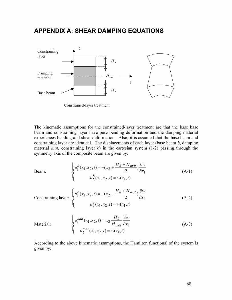
APPENDIX A: SHEAR DAMPING EQUATIONS

Dampingmaterial

Base beam

matH

bH

bH

Constrained-layer treatment

1

2Constraininglayer

The kinematic assumptions for the constrained-layer treatment are that the base base beam and constraining layer have pure bending deformation and the damping material experiences bending and shear deformation. Also, it is assumed that the base beam and constraining layer are identical. The displacements of each layer (base beam b, damping material mat, constraining layer c) in the cartesian system (1-2) passing through the symmetry axis of the composite beam are given by:

Beam:

=∂∂+

+−=

),(),,(

)2

(),,(

1212

12211

txwtxxuxwHH

xtxxu

b

matbb (A-1)

Constraining layer:

=∂∂+

−−=

),(),,(

)2

(),,(

1212

12211

txwtxxuxwHH

xtxxu

c

matbc (A-2)

Material:

=∂∂

=

),(),,(

),,(

1212

12211

txwtxxuxw

HH

xtxxu

matmat

bmat (A-3)

According to the above kinematic assumptions, the Hamilton functional of the system is given by:

68

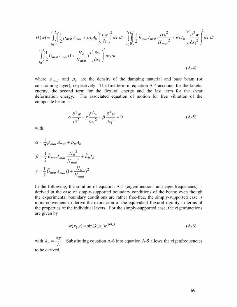
dtdxxw

HH

AG

dtdxx

wIEH

HIEdtdx

twAAwH

t

t

L

mat

bmatmat

t

t

L

bbmat

bmatmat

t

t

L

bbmatmat

10

2

1

2

10

2

21

2

2

2

01

2

1

0

1

0

1

0

)1(~21

~~21

21)(

∫ ∫

∫ ∫∫ ∫

∂∂

+−

∂

∂

+−

∂∂

+= ρρ

(A-4) where matρ and bρ are the density of the damping material and base beam (or constraining layer), respectively. The first term in equation A-4 accounts for the kinetic energy, the second term for the flexural energy and the last term for the shear deformation energy. The associated equation of motion for free vibration of the composite beam is:

041

4

21

2

2

2=

∂

∂+

∂

∂−

∂

∂

xw

xw

tw βγα (A-5)

with:

2

2

2

)1(~21

~~2121

mat

bmatmat

bbmat

bmatmat

bbmatmat

HH

AG

IEH

HIE

AA

+=

+=

+=

γ

β

ρρα

In the following, the solution of equation A-5 (eigenfunctions and eigenfrequencies) is derived in the case of simply-supported boundary conditions of the beam; even though the experimental boundary conditions are rather free-free, the simply-supported case is more convenient to derive the expression of the equivalent flexural rigidity in terms of the properties of the individual layers. For the simply-supported case, the eigenfunctions are given by (A-6) tj

n nexktxw ω)sin(),( 11 =

with L

nknπ

= . Substituting equation A-6 into equation A-5 allows the eigenfrequencies

to be derived,

69

bbmatmat

nbbmat

bmatmat

mat

bmatmat

nn

nnAA

kIEH

HIE

HH

AG

kk

kρρα

βγω

+

+++

=+

=

21

~~21)1(~

21 2

2

22

2

(A-7) In most cases, the damping material has a much lower rigidity than the base or

constraining layer, such that bbmat

bmatmat IE

H

HIE ~~

2

2<< , and equation A-7 can be

simplified to

bbmatmat

nbbmat

bmatmat

nnAA

kIEHH

AGk

ρρω

+

++=

21

~)1(~21 22

(A-8)

The equivalent flexural rigidity of the composite beam IE~ can be deduced by identifying

equation A-8 with bbmatmat

nn AAIEk

ρρω

2

~2

+= . It follows that

bbnmat

bmatmat IEk

HH

AGIE ~2/)1(~~ 22 ++= (A-9)

70

APPENDIX B: Theory-experiment comparison for various material characterisation data • 2mm steel plate + 3mm neoprene foam

Shear damping Extensional damping

Experimental

Figure B.1: Mean square velocity on airside of the 2mm steel plate + 3mm neoprene foam (1/3 octave results) , comparison between experimental results and VIBRO1D with material properties derived from extensional or shear damping measurements.

Experimental

Extensional damping

Shear damping

Figure B.2: Mean square velocity on water side of the 2mm steel plate + 3mm neoprene foam (1/3 octave results) , comparison between experimental results and VIBRO1D with material properties derived from extensional or shear damping measurements.

71

DREA dataShear damping

Extensional damping

Experimental

Figure B.3: Mean square velocity ratio (airside/waterside) of the 2mm steel plate + 3mm neoprene foam (1/3 octave results) , comparison between experimental results and VIBRO3D with material properties derived from extensional measurements, shear damping measurements or DREA data.

Experimental

DREA data Shear damping

Figure B.4: Mean square velocity on airside of the 2mm steel pneoprene foam (1/3 octave results) , comparison between experand VIBRO3D with material properties derived from extensionshear damping measurements or DREA data.

Extensional damping

late + 3mm imental results al measurements,

72

DREA data Extensional damping

Shear damping

Experimental

Figure B.5: Mean square velocity on waterside of the 2mm steel plate + 3mm neoprene foam (1/3 octave results) , comparison between experimental results and VIBRO3D with material properties derived from extensional measurements, shear damping measurements or DREA data.

Experim

Shear damping TNO data

Figure B.6: Mean square velocity ratio (water side/airside) of + 3mm neoprene foam (1/3 octave results) , comparison betweresults and VIBRO3D with material properties derived from exmeasurements, shear damping measurements and TNO data.

Extensionaldamping

ental

the 2mm steel plate en experimental tensional

73

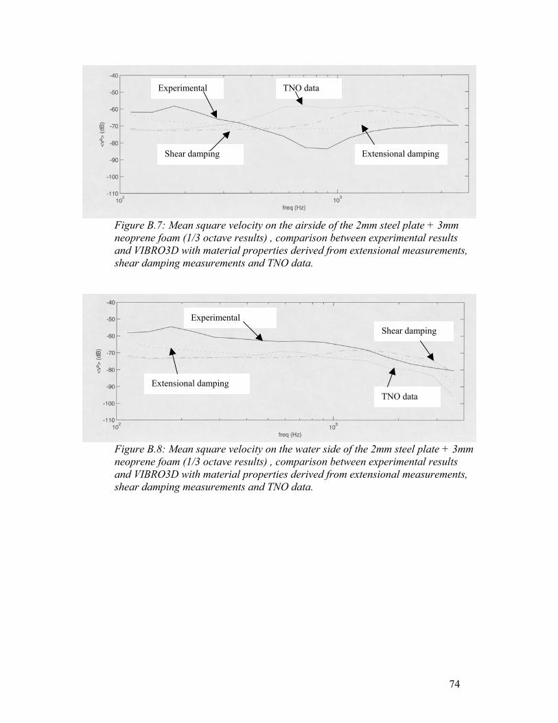
Experimental TNO data

Extensional damping Shear damping

Figure B.7: Mean square velocity on the airside of the 2mm steel plate + 3mm neoprene foam (1/3 octave results) , comparison between experimental results and VIBRO3D with material properties derived from extensional measurements, shear damping measurements and TNO data.

Experimental Shear damping

Extensional damping TNO data

Figure B.8: Mean square velocity on the water side of the 2mm steel plate + 3mm neoprene foam (1/3 octave results) , comparison between experimental results and VIBRO3D with material properties derived from extensional measurements, shear damping measurements and TNO data.

74

• 2mm steel plate + 6mm EVA foam

Shear damping

Experimental Extensional damping

Figure B.9: Mean square velocity on airside of the 2mm steel plate + 6mm EVA foam (1/3 octave results) , comparison between experimental results and VIBRO1D with material properties derived from extensional or shear damping measurements.

Extensional damping

Experimental

Shear damping

Figure B.10: Mean square velocity on water side of the 2mm steel plate + 6mm EVA foam (1/3 octave results) , comparison between experimental results and VIBRO1D with material properties derived from extensional or shear damping measurements.

75

Shear damping DREA data

Extensionaldamping

Experimental

Figure B.11: Mean square velocity ratio (airside/waterside) of the 2mm steel plate + 6mm EVA foam (1/3 octave results) , comparison between experimental results and VIBRO3D with material properties derived from extensional measurements, shear damping measurements or DREA data.

Shear damping Experimental DREA data

Extensional damping

Figure B.12: Mean square velocity on airside of the 2mm steel plate + 6mm EVA foam (1/3 octave results) , comparison between experimental results and VIBRO3D with material properties derived from extensional measurements, shear damping measurements or DREA data.

76

Shear damping Experimental

Extensional dampingDREA data

Figure B.13: Mean square velocity on water side of the 2mm steel plate + 6mm EVA foam (1/3 octave results) , comparison between experimental results and VIBRO3D with material properties derived from extensional measurements, shear damping measurements or DREA data.

Shear damping GIL data

Experimental

Figure B.14: Mean square velocity ratio (water side/airside) of thplate + 6mm EVA foam (1/3 octave results) , comparison betweenresults and VIBRO3D with material properties derived from extenmeasurements, shear damping measurements and GIL data.

Extensionaldamping

e 2mm steel experimental sional

77

Extensional dampingExperimental GIL data

Shear damping

Figure B.15: Mean square velocity on the airside of the 2mm steel plate + 6mm EVA foam (1/3 octave results) , comparison between experimental results and VIBRO3D with material properties derived from extensional measurements, shear damping measurements and GIL data.


Extensional damping GIL data

Figure B.16: Mean square velocity on the water side of the 2mm steel plate + 6mm EVA foam (1/3 octave results) , comparison between experimental results and VIBRO3D with material properties derived from extensional measurements, shear damping measurements and GIL data.

78

• 9.5mm steel plate + 25 EPT foam

Extensional damping Experimental

Figure B.17: Mean square velocity on airside of the 9.5mm steel plate + 25mm EPT foam (1/3 octave results) , comparison between experimental results and VIBRO1D with material properties derived from extensional or shear damping measurements.

Shear damping

Experimental

Extensional dampingShear damping

Figure B.18: Mean square velocity on water side of the 9.5mm steel plate + 25mm EPT foam (1/3 octave results) , comparison between experimental results and VIBRO1D with material properties derived from extensional or shear damping measurements.

79

Extensional damping


Figure B.19: Mean square velocity ratio (airside/water side) of the 9.5mm steel plate + 25mm EPT foam (1/3 octave results) , comparison between experimental results and VIBRO1D with material properties derived from extensional measurements, and shear damping measurements.

GIL data

Shear damping

Experimental

Figure B.20: Mean square velocity ratio (waterside/air side) of tplate + 25mm EPT foam (1/3 octave results) , comparison betweresults and VIBRO3D with material properties derived from extemeasurements, shear damping measurements and GIL data.

Extensionaldamping

he 9.5mm steel en experimental nsional

80

GIL data Experimental Shear damping

Figure B.21: Mean sq25mm EPT foam (1/3 and VIBRO3D with mshear damping measur

Experimental

GIL data

Figure B.22: Mean sq25mm EPT foam (1/3 and VIBRO3D with mshear damping measur

Extensional damping

uare velocity on the airside of the 9.5mm steel plate + octave results) , comparison between experimental results aterial properties derived from extensional measurements, ements and GIL data.

Shear damping

Extensional damping

uare velocity on the water side of the 9.5mm steel plate + octave results) , comparison between experimental results aterial properties derived from extensional measurements, ements and GIL data.

81

Extensionaldamping

Experimental Shear damping

DREA data

Figure B.23: Mean square velocity on the water side of the 9.5mm steel plate + 25mm EPT foam (1/3 octave results) , comparison between experimental results and VIBRO3D with material properties derived from extensional measurements, shear damping measurements and DREA data.

82

83

APPENDIX C: Influence of the volume of water on the vibration response

Full tank

Half tank

Figure C: Mean square velocity ratio on the water side of the 2mm steel plate + 3mm neoprene foam (1/3 octave results) , with 2 different water volumes in the tank.

84


VIBRO Software Experimental Validation - Defence...

Documents

Transcript of VIBRO Software Experimental Validation - Defence...