VIBRATIONAL ANALYSIS OF VERTICAL AXIS WIND TURBINE BLADES ... · vibrational analysis of vertical...

VIBRATIONAL ANALYSIS OF VERTICAL AXIS WIND TURBINE BLADES

By

Onur Kapucu

A THESIS

Submitted toMichigan State University

in partial fulfillment of the requirementsfor the degree of

Mechanical Engineering - Master of Science

2014

ABSTRACT

VIBRATIONAL ANALYSIS OF VERTICAL AXIS WIND TURBINE BLADES

By

Onur Kapucu

The goal of this research is to derive a vibration model for a vertical axis wind turbine

blade. This model accommodates the affects of varying relative flow angle caused by rotating

the blade in the flow field, uses a simple aerodynamic model that assumes constant wind

speed and constant rotation rate, and neglects the disturbance of wind due to upstream blade

or post. The blade is modeled as elastic Euler-Bernoulli beam under transverse bending

and twist deflections. Kinetic and potential energy equations for a rotating blade under

deflections are obtained, expressed in terms of assumed modal coordinates and then plugged

into Lagrangian equations where the non-conservative forces are the lift and drag forces and

moments. An aeroelastic model for lift and drag forces, approximated with third degree

polynomials, on the blade are obtained assuming an airfoil under variable angle of attack

and airflow magnitudes. A simplified quasi-static airfoil theory is used, in which the lift and

drag coefficients are not dependent on the history of the changing angle of attack. Linear

terms on the resulting equations of motion will be used to conduct a numerical analysis and

simulation, where numeric specifications are modified from the Sandia-17m Darrieus wind

turbine by Sandia Laboratories.

Copyright byONUR KAPUCU2014

I would like to dedicate this work to my mother Gonca Kapucu and my father AliKapucu.

iv

ACKNOWLEDGMENTS

I would like to thank my advisor and my master Professor Brian Feeny for his endless

technical and mental support and sharing his wisdom generously to influence me to go

further. Without his dedication this research would have never existed.

I would also like to thank dear Katy Luchini Colbry, for always being there to listen and

help me.

v

TABLE OF CONTENTS

LIST OF TABLES . . . . . . . . . . . . . . . . . . . . . . . . . . . . . . . . . . . . vii

LIST OF FIGURES . . . . . . . . . . . . . . . . . . . . . . . . . . . . . . viii

Chapter 1 Introduction . . . . . . . . . . . . . . . . . . . . . . . . . . . . . . . . 11.1 Background . . . . . . . . . . . . . . . . . . . . . . . . . . . . . . . . . . . . 1

1.1.1 Efficiency . . . . . . . . . . . . . . . . . . . . . . . . . . . . . . . . . 41.1.2 Blade Dynamics . . . . . . . . . . . . . . . . . . . . . . . . . . . . . . 51.1.3 Installation . . . . . . . . . . . . . . . . . . . . . . . . . . . . . . . . 5

1.2 Motivation . . . . . . . . . . . . . . . . . . . . . . . . . . . . . . . . . . . . . 61.3 Objective . . . . . . . . . . . . . . . . . . . . . . . . . . . . . . . . . . . . . 81.4 Contribution . . . . . . . . . . . . . . . . . . . . . . . . . . . . . . . . . . . . 81.5 Thesis Outline . . . . . . . . . . . . . . . . . . . . . . . . . . . . . . . . . . . 8

Chapter 2 Formulation and Modeling . . . . . . . . . . . . . . . . . . . . . . . 102.1 Elastic Blade Model for Bending . . . . . . . . . . . . . . . . . . . . . . . . . 102.2 Reduced Order Modeling . . . . . . . . . . . . . . . . . . . . . . . . . . . . . 142.3 Aeroelastic Modeling . . . . . . . . . . . . . . . . . . . . . . . . . . . . . . . 172.4 Linearization . . . . . . . . . . . . . . . . . . . . . . . . . . . . . . . . . . . 25

Chapter 3 Numerical Analysis and Simulation . . . . . . . . . . . . . . . . . 273.1 Definition of the Giromill/H-Rotor Blade . . . . . . . . . . . . . . . . . . . . 273.2 Modal Frequencies . . . . . . . . . . . . . . . . . . . . . . . . . . . . . . . . 313.3 Blade with Quasistatic Aeroelastic Airfoil Model . . . . . . . . . . . . . . . . 32

Chapter 4 Conclusion and Comments . . . . . . . . . . . . . . . . . . . . . . . 354.1 Summary of Results . . . . . . . . . . . . . . . . . . . . . . . . . . . . . . . 354.2 Contribution . . . . . . . . . . . . . . . . . . . . . . . . . . . . . . . . . . . . 364.3 Future Work . . . . . . . . . . . . . . . . . . . . . . . . . . . . . . . . . . . . 36

APPENDIX . . . . . . . . . . . . . . . . . . . . . . . . . . . . . . . . . . 38

BIBLIOGRAPHY . . . . . . . . . . . . . . . . . . . . . . . . . . . . . . . . . . . 72

vi

LIST OF TABLES

Table 3.1 Selected aluminium alloy’s material properties . . . . . . . . . . . . 30

Table 3.2 Specifications of the model created . . . . . . . . . . . . . . . . . . . 31

vii

LIST OF FIGURES

Figure 1.1 A sample HAWT sketch on left[2] and VAWT sketch on right [3] . . 2

Figure 1.2 A sample sketch for a Savonius WT on the left, Darrieus WT in themiddle and H-rotor configuration on the right [5] . . . . . . . . . . . 3

Figure 1.3 Comparison of aerodynamic efficiencies of different wind turbine types[10] . . . . . . . . . . . . . . . . . . . . . . . . . . . . . . . . . . . . 4

Figure 1.4 Basic VAWT Configurations: (a) Full Darrieus, (b)“H” , (c) “V”, (d)“∆”, (e) “Diamond” and (f) “Giromill”[6] . . . . . . . . . . . . . . . 7

Figure 2.1 A sketch of blade and rotor. Undeformed on left and deformed onright. . . . . . . . . . . . . . . . . . . . . . . . . . . . . . . . . . . . 12

Figure 2.2 Top view representation of transverse deflection on top and twist onbottom. . . . . . . . . . . . . . . . . . . . . . . . . . . . . . . . . . . 15

Figure 2.3 Cross section of VAWT showing the coordinate axes . . . . . . . . . 18

Figure 2.4 Twist angle ψ and relative wind angle φ for the case when the pretwistβ = 0 . . . . . . . . . . . . . . . . . . . . . . . . . . . . . . . . . . . 19

Figure 2.5 Lift and drag force per unit length directions from top view . . . . . 20

Figure 2.6 NACA0012 CL and CD values with respect to angle of attack [21] . 21

Figure 3.1 Sandia 17m front view . . . . . . . . . . . . . . . . . . . . . . . . . 28

Figure 3.2 Sandia 17m blade cross section showing aluminum spar and spline,Nomex core and fiberglass skin. [22] . . . . . . . . . . . . . . . . . . 29

Figure 3.3 Blade dimensions for calculations . . . . . . . . . . . . . . . . . . . 29

Figure 3.4 Variation of wnq with Ω on left and blade length a on right . . . . . 32

Figure 3.5 Variation of wnq and wnb with a when Ω = 0 . . . . . . . . . . . . . 33

Figure 3.6 Rotor dimensions used in calculations . . . . . . . . . . . . . . . . . 34

viii

Chapter 1

Introduction

1.1 Background

Our society’s increasing demand on energy has reached a critical level where the future

projections show us our fossil fuel sources will not be able to supply the demand in near

future. Being only dependent on several energy sources makes humankind vulnerable to en-

ergy shortage. Moreover, fossil fuel dependence in energy production unnaturally empowers

countries with rich fossil sources and increases the tension of international politics.

These facts show us the importance of the search for renewable energy sources. Being

aware of the aforementioned facts, most countries are now challenging a productive compe-

tition to develop and master the energy sources of the future. Facing the exhaustion of fossil

sources, we are spending more effort to exploit renewable sources such as wind, solar energy,

geothermal energy.

Among the renewable energy alternatives, wind power is a popular player. Energy Infor-

mation Administration’s Annual Energy Outlook 2014[1] reference case projects 76% increase

in electricity production from wind power by 2040, where this increase is more than 300% in

the extended policies case. There exist several ways to absorb wind power and convert it into

a useful energy form. Wind turbines are the most popular setups to accomplish this purpose.

They basically convert the power of the wind into electricity via rotation in the generator.

Wind turbines can be distinguished into two main classes depending on the orientation of

1

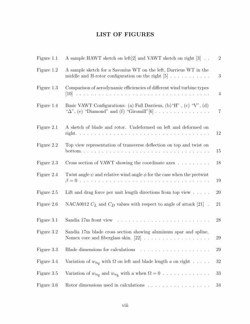
the rotor: horizontal axis wind turbines (HAWTs) and vertical axis wind turbines (VAWTs).

In this notation “axis” represents the axis of rotation of rotor. Axes of rotation of VAWT

rotors are perpendicular to the ground, where they are parallel to ground in HAWT blades.

See Figure 1.1.

Figure 1.1 A sample HAWT sketch on left[2] and VAWT sketch on right [3]

Horizontal axis wind turbines dominate the current market; however, this might simply

be a coincidence [4]. The most common HAWT configuration has its blades facing the wind

to generate a rotation as a result of the lift forces on the blades. Being widely used, they

can be seen in various sizes from stand-alone installations to offshore fleets. As the energy

demand has increased over the time, HAWTs have become larger to produce more energy

from a single turbine. As of 2014, tallest commercial HAWT (MHI VESTAS V164) reaches

a tower height of 140 meters with a 220 meter tip height and 82 meter blade length and can

generate 8MW energy. Yet, as HAWT sizes have increased, problems with installation and

durability also have arisen. This might be a limiting factor for the future of the HAWTs [5].

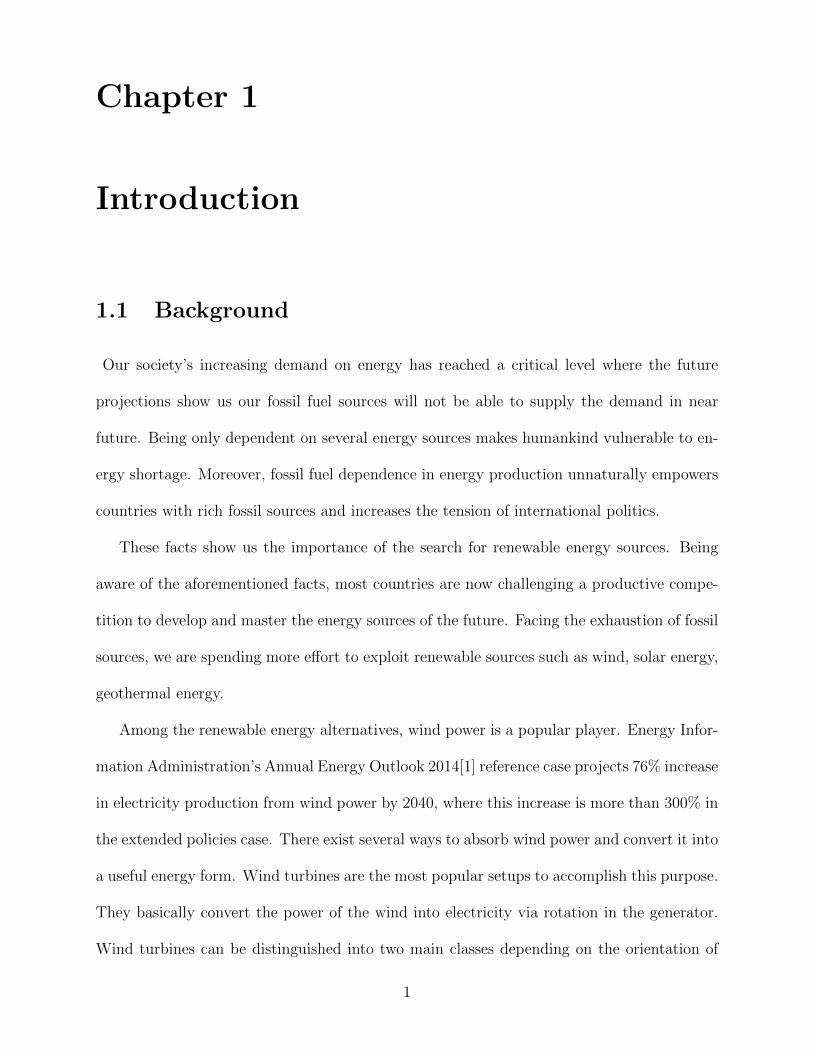
The second most common wind turbine configuration, the VAWT, has its blades rotating

around a vertical axis. We can group VAWTs mainly into two: ones using lift-momentum

airfoils (i.e. Darrieus wind turbines) and ones using drag cups (Savonius wind turbine)(See

Figure 1.2). Among these there exist numerous configurations; such as, the Giromill/H-

2

rotor configurations, which are common types of Darrieus Turbine, due their simplicity.

Giromill/H-rotor style VAWTs consist of simply designed airfoils attached parallel to the

rotor via several struts or a single strut.

Figure 1.2 A sample sketch for a Savonius WT on the left, Darrieus WT in the middle andH-rotor configuration on the right [5]

Our most significant experience with commercial VAWT installations dates back to the

early 80’s [5, 6]. Manufacturer FloWind initiated a large operation to install Darrieus type

VAWTs in the California Altamont and Tehachipi Wind Farms. The company installed more

than 500 turbines and reached a maximum total production of 105,000 megawatt/hour in

1987. However, shortly after this, the turbine fleet began collapsing due to failures in the

connection parts of the aluminum blades. By the late 90’s, their energy production decreased

down to 10,000 megawatt/hour and whole fleet was removed in early 2000’s. Nonetheless, a

thorough investigation of the blade dynamics was not conducted.

Next is a comparison of HAWTs and VAWTs in terms of efficiency, blade dynamics and

installation features.

3

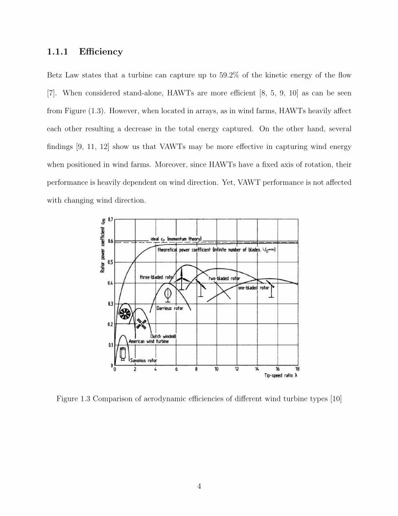
1.1.1 Efficiency

Betz Law states that a turbine can capture up to 59.2% of the kinetic energy of the flow

[7]. When considered stand-alone, HAWTs are more efficient [8, 5, 9, 10] as can be seen

from Figure (1.3). However, when located in arrays, as in wind farms, HAWTs heavily affect

each other resulting a decrease in the total energy captured. On the other hand, several

findings [9, 11, 12] show us that VAWTs may be more effective in capturing wind energy

when positioned in wind farms. Moreover, since HAWTs have a fixed axis of rotation, their

performance is heavily dependent on wind direction. Yet, VAWT performance is not affected

with changing wind direction.

Figure 1.3 Comparison of aerodynamic efficiencies of different wind turbine types [10]

4

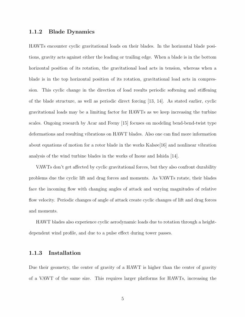
1.1.2 Blade Dynamics

HAWTs encounter cyclic gravitational loads on their blades. In the horizontal blade posi-

tions, gravity acts against either the leading or trailing edge. When a blade is in the bottom

horizontal position of its rotation, the gravitational load acts in tension, whereas when a

blade is in the top horizontal position of its rotation, gravitational load acts in compres-

sion. This cyclic change in the direction of load results periodic softening and stiffening

of the blade structure, as well as periodic direct forcing [13, 14]. As stated earlier, cyclic

gravitational loads may be a limiting factor for HAWTs as we keep increasing the turbine

scales. Ongoing research by Acar and Feeny [15] focuses on modeling bend-bend-twist type

deformations and resulting vibrations on HAWT blades. Also one can find more information

about equations of motion for a rotor blade in the works Kalsøe[16] and nonlinear vibration

analysis of the wind turbine blades in the works of Inoue and Ishida [14].

VAWTs don’t get affected by cyclic gravitational forces, but they also confront durability

problems due the cyclic lift and drag forces and moments. As VAWTs rotate, their blades

face the incoming flow with changing angles of attack and varying magnitudes of relative

flow velocity. Periodic changes of angle of attack create cyclic changes of lift and drag forces

and moments.

HAWT blades also experience cyclic aerodynamic loads due to rotation through a height-

dependent wind profile, and due to a pulse effect during tower passes.

1.1.3 Installation

Due their geometry, the center of gravity of a HAWT is higher than the center of gravity

of a VAWT of the same size. This requires larger platforms for HAWTs, increasing the

5

material weight and cost. As stated in the Sandia Workshop of 2012, VAWTs might be more

advantageous in off-shore installations for this and a variety of other reasons [5].

1.2 Motivation

The following facts motivate the need of a comprehensive research in VAWTs [17]:

1. Not being the primary contributor of its market, our knowledge and experience with

VAWT dynamics is limited.

2. Despite all of the efforts and research, large scaled HAWTs suffer failures due cyclic

gravitational and aerodynamic effects. Therefore, being heavily dependent on HAWTs might

be a bottleneck for the future of wind power. VAWTs might reach larger scales and therefore

produce higher stand-alone energy rates in the future. Furthermore, VAWTs may perform

better in arrays[9].

3. Known durability problems for VAWT blades are outdated and might be overcome

with modern material and production technologies if investigated further.

4. A better understanding of VAWT dynamics might help us to prove and improve better

off-shore wind power generation capacities.

5. Efficiency of stand-alone VAWTs might be improved with different blade configurations

combining lift-momentum and drag cup.

However, as stated in a recent Sandia Report [5], VAWT technology is still open to

development and research in the following areas can be conducted to broaden our knowledge

and widen its usage.

1. Aerodynamics: Generally typical NACA blades are used in VAWTs. Improved aerody-

namic analysis of turbines will help us find optimized blade solutions which can significantly

6

improve turbine efficiency. Similarly struts and joints can be optimized to improve perfor-

mance.

2. Materials, drive train: Failures of VAWT blades in the 80’s in California are thought

to be related to the aluminum blade and joints. Further analysis of loads and vibrations

in VAWTs combined with the improvements in the material science may open the path for

durable VAWTs that can be scaled larger than HAWTs. Furthermore, once the loads and

vibrations are modeled, optimal drivetrain architecture can be developed.

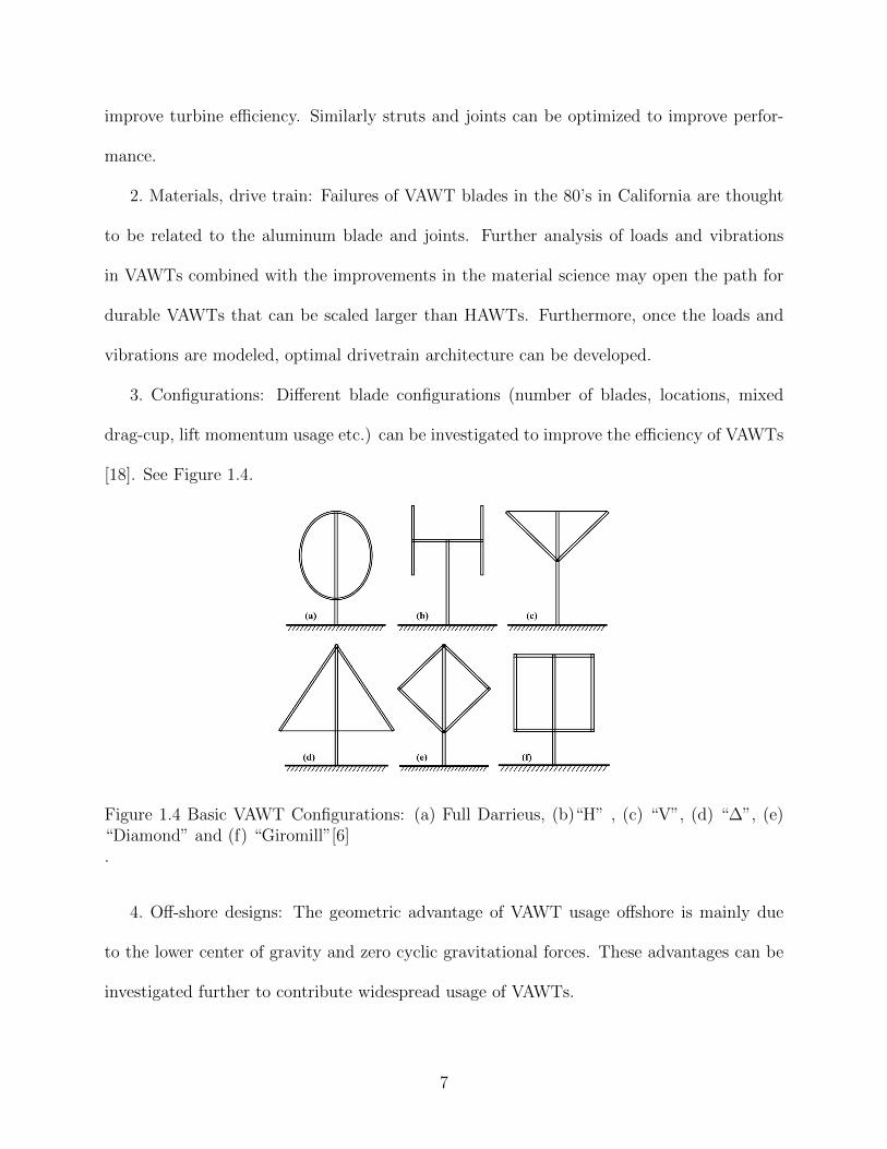
3. Configurations: Different blade configurations (number of blades, locations, mixed

drag-cup, lift momentum usage etc.) can be investigated to improve the efficiency of VAWTs

[18]. See Figure 1.4.

Figure 1.4 Basic VAWT Configurations: (a) Full Darrieus, (b)“H” , (c) “V”, (d) “∆”, (e)“Diamond” and (f) “Giromill”[6].

4. Off-shore designs: The geometric advantage of VAWT usage offshore is mainly due

to the lower center of gravity and zero cyclic gravitational forces. These advantages can be

investigated further to contribute widespread usage of VAWTs.

7

1.3 Objective

This research aims to derive a vibration model that accommodates the affects of varying

relative flow angle within a simple aerodynamic model. Throughout the research, a straight

vertical airfoil, such as the ones in H-Rotor and Giromill configured VAWTs, will be the

target of our interest. It will be supported by two struts located at the ends of the blade;

still, it can be modified easily for other locations on the blade.

1.4 Contribution

This research aims to contribute

1. A simple model of VAWT blade vibration, which currently does not seem to exist.

This two-mode model will consist of a pair of 2nd-order ODEs that are cyclically forced and

parametrically excited.

2. The model will be formulated to include up to cubic nonlinearity.

3. The ODEs will have many terms whose coefficients will be defined in a table of formulas

that will be provided.

4. This work serves to set up the follow-up research which will involve analysis and

numerical simulations.

1.5 Thesis Outline

In the upcoming chapters:

1. Energies for deriving nonlinear partial differential equations of the vibration of a single

blade will be obtained for one-dimensional transverse bending and twist.

8

2. A simplified aeroelastic model will be introduced based on semi-empirical quasi-static

airfoil theory.

3. Single assumed modes for transverse bending and twist will be used to reduce the order

of equations in the model. Two ordinary differential equations representing bend and twist

will be derived using Lagrange’s equations. The equations will be linearized relative to the

undeformed state.

4. A numerical evaluation of equation coefficients will be made for a specifically defined

turbine blade, resulting in equations that are dependent on few parameters, such as ro-

tation frequency and blade length. Since data for an existing H-rotor/Giromill turbine is

not available, we will use data from a Sandia 17m Darrieus turbine as a guide for our H-

rotor/Giromill model. The numerical evaluation will include an estimate of the first-mode

natural frequency, as a function of blade length, for the non rotating blade. The aeroelastic

terms will be based on a NACA0012 symmetric airfoil.

9

Chapter 2

Formulation and Modeling

We derive a vibration model for an H-rotor/Giromill blade. The blade is treated as a

uniform straight beam under bending and twisting deformations.

This chapter can be presented in several parts. First comes the derivation of the energy

equations for the bending and twisting blade. It will be followed by a simplified aerodynamic

model to obtain the lift and drag force and moment equations as functions of time and spatial

location on the blade.

Before going forward with modeling several assumptions were made:

1. Steady wind speed

2. Neglect the disturbance of wind due to upstream blade or post

3. Constant (steady-state) rotation rate

4. Inextensible beam

5. Shear center is at the geometric center of the blade

2.1 Elastic Blade Model for Bending

Following the ideas of Feeny [17] we will model our blades as an elastic Euler-Bernoulli beam.

A blade that we model could face bend-bend-twist deflections, yet only one-dimensional

transverse bending and twist will be taken into consideration for the rest of the formulation

and modeling. Here transverse bending is the deflection of the blade to the radial direction,

10

and twist occurs around the axis that passes through the centroid of the blade cross sections.

First, kinetic and potential energy equations for the particles on the beam will be ex-

pressed such that the extended Hamilton’s principle can be used to obtain the partial differ-

ential equations of motion. Alternatively, a Lagrange formulation based on assumed modes

can be applied to the energy formulations.

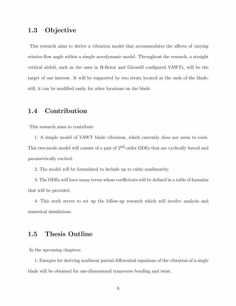
In order to do so, sections along the undeformed beam axis will be located from an origin

at the middle center of the rotor using the following position vector:

r(x, t) = (x− s(x, t))i + (R + y(x, t))er (2.1)

See Figure 2.1 and Figure 2.2.

In this equation, R is the distance between undeformed beam and the axis of rotation,

x is the vertical distance of the blade section to the origin, y(x, t) is the radially transverse

displacement of the selected section on beam at time t, s(x, t) is the cumulative foreshortening

affecting point x at time t, due deflection. The foreshortening term, s, is formulated to be

positive for x > 0. Also i is a unit vector in the direction in the undeformed x axis and er

is a unit vector in the direction in the y axis, radial to the center of rotation.

We can also formulate the foreshortening for an Euler-Bernoulli beam due to one di-

mensional transverse bending in the radial direction y to retain up to 4th degree terms, as

[13]

s(x, t) ∼=∫ +a

−a(y′2

2+y′4

8)dz, (2.2)

which will contribute linear and cubic terms to the equations of motion where a is half

the length of the blade. Assuming constant rotational speed and neglecting the effects of

transverse deflection in the circumferential direction on the energy, the kinetic energy for

11

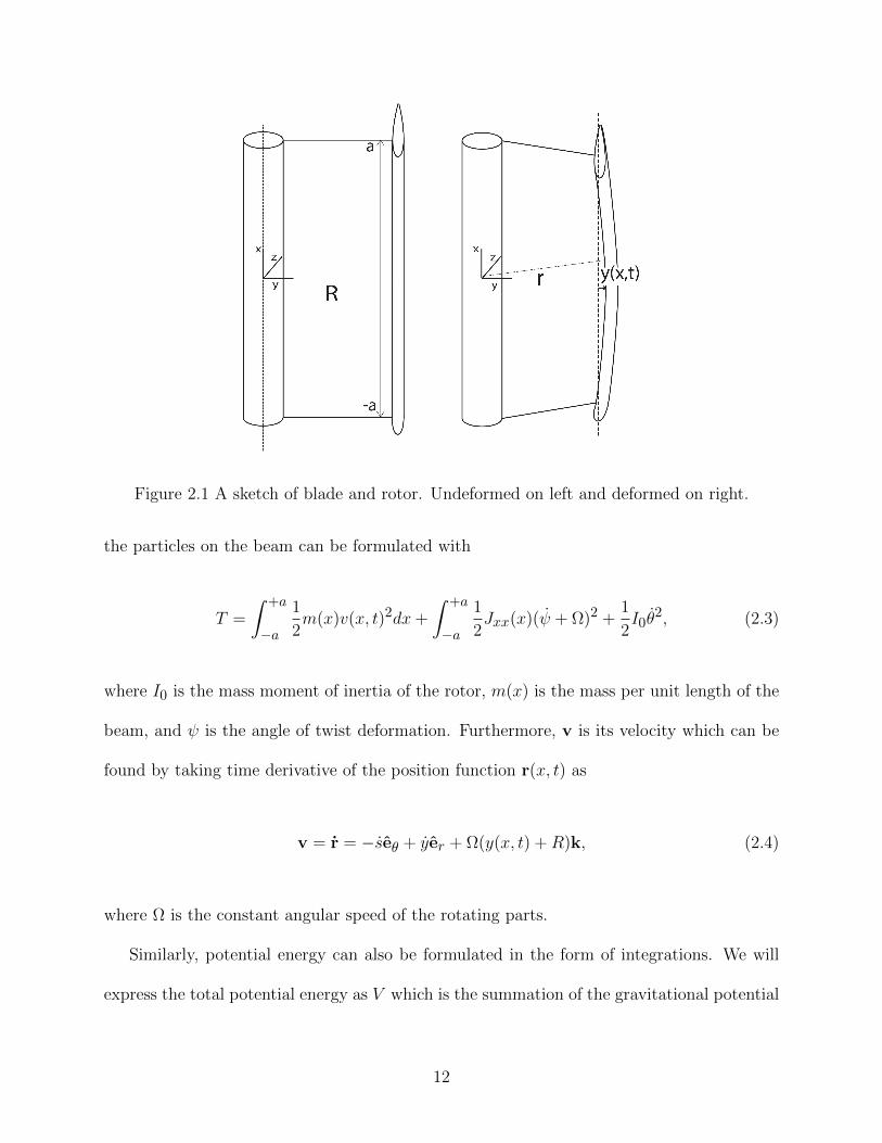
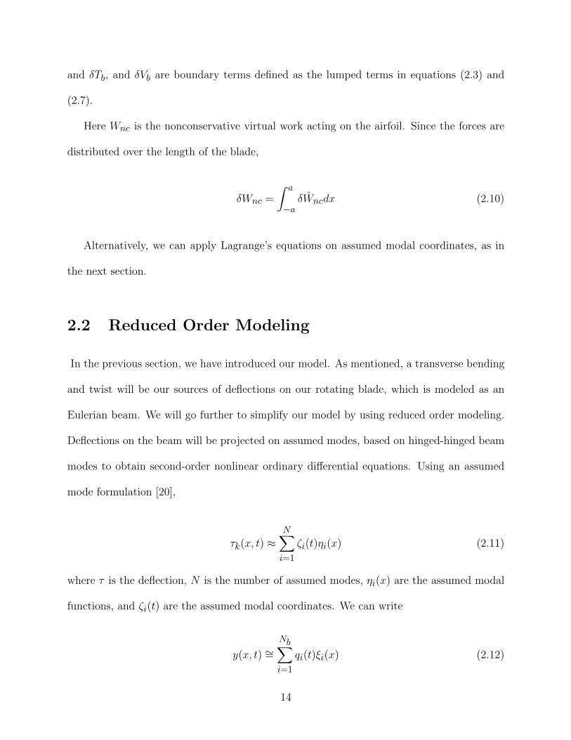
Figure 2.1 A sketch of blade and rotor. Undeformed on left and deformed on right.

the particles on the beam can be formulated with

T =

∫ +a

−a

1

2m(x)v(x, t)2dx+

∫ +a

−a

1

2Jxx(x)(ψ + Ω)2 +

1

2I0θ

2, (2.3)

where I0 is the mass moment of inertia of the rotor, m(x) is the mass per unit length of the

beam, and ψ is the angle of twist deformation. Furthermore, v is its velocity which can be

found by taking time derivative of the position function r(x, t) as

v = r = −seθ + yer + Ω(y(x, t) +R)k, (2.4)

where Ω is the constant angular speed of the rotating parts.

Similarly, potential energy can also be formulated in the form of integrations. We will

express the total potential energy as V which is the summation of the gravitational potential

12

energy, Vmg, strain energy due bending and twist, Vs, and the elastic potential energy of the

boundaries of the beam, Vb.

As such, neglecting net vertical deflections of the blade, we have

Vmg =

∫ +a

−am(x)gs(x, t)dx, (2.5)

Vs =

∫ +a

−a

1

2EIz(x)[y′′2(1− 3y′2)]dx+

∫ +a

−a

1

2GIx(x)ψ′2dx, (2.6)

Vb =1

2k1(ug − s(−a, t))2 +

1

2kT1

(y′(−a, t))2 +1

2k2(ug − s(a, t))2 +

1

2kT2

(y′(a, t))2, (2.7)

where E is the Young’s modulus, and Iz(x) is the area moment of inertia of the cross

section at x about the neutral axis. Vs includes effects of nonlinear bending curvature [19]

approximated to 4th degree. Also one should note that elastic modeling has two parts for

each strut. Struts are modeled as superposed linear and torsional springs where linear spring

constants are k1 and k2, torsional spring constants are kT1and kT2

for struts 1 and 2. In

order to simplify the model, k1 is assumed to be equal to k2 and kT1is assumed to be equal

to kT2.

The extended Hamilton’s principle can be used to obtain partial differential equations of

motion. Hamilton’s principle states that

∫ t2

t1

(δT − δV + δWnc)dt = 0 (2.8)

or ∫ t2

t1

(∫ L

0(δT − δV + δ Wnc)dx+ δTb − δVb + δWncb

)dt = 0 (2.9)

where δT , δV are energy densities, defined as the integrands in eqns (2.3), (2.5) and (2.6),

13

and δTb, and δVb are boundary terms defined as the lumped terms in equations (2.3) and

(2.7).

Here Wnc is the nonconservative virtual work acting on the airfoil. Since the forces are

distributed over the length of the blade,

δWnc =

∫ a

−aδWncdx (2.10)

Alternatively, we can apply Lagrange’s equations on assumed modal coordinates, as in

the next section.

2.2 Reduced Order Modeling

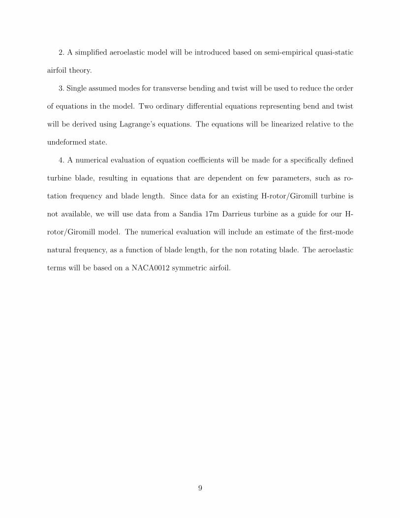
In the previous section, we have introduced our model. As mentioned, a transverse bending

and twist will be our sources of deflections on our rotating blade, which is modeled as an

Eulerian beam. We will go further to simplify our model by using reduced order modeling.

Deflections on the beam will be projected on assumed modes, based on hinged-hinged beam

modes to obtain second-order nonlinear ordinary differential equations. Using an assumed

mode formulation [20],

τk(x, t) ≈N∑i=1

ζi(t)ηi(x) (2.11)

where τ is the deflection, N is the number of assumed modes, ηi(x) are the assumed modal

functions, and ζi(t) are the assumed modal coordinates. We can write

y(x, t) ∼=Nb∑i=1

qi(t)ξi(x) (2.12)

14

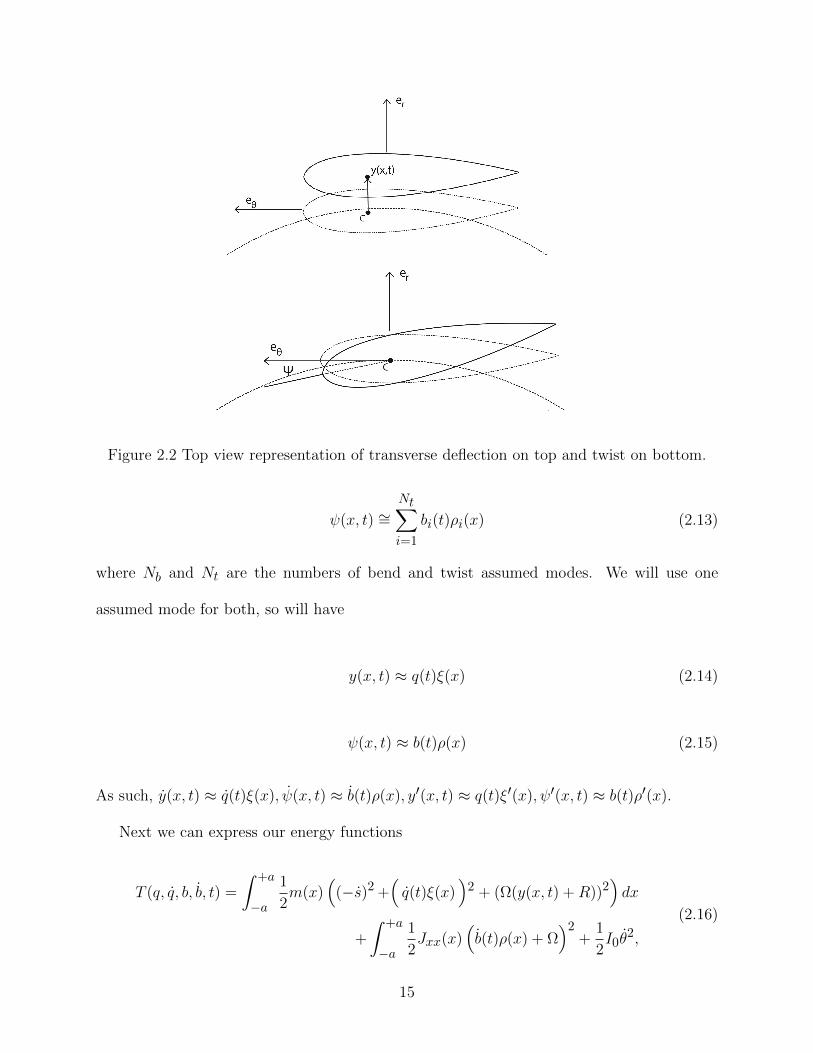
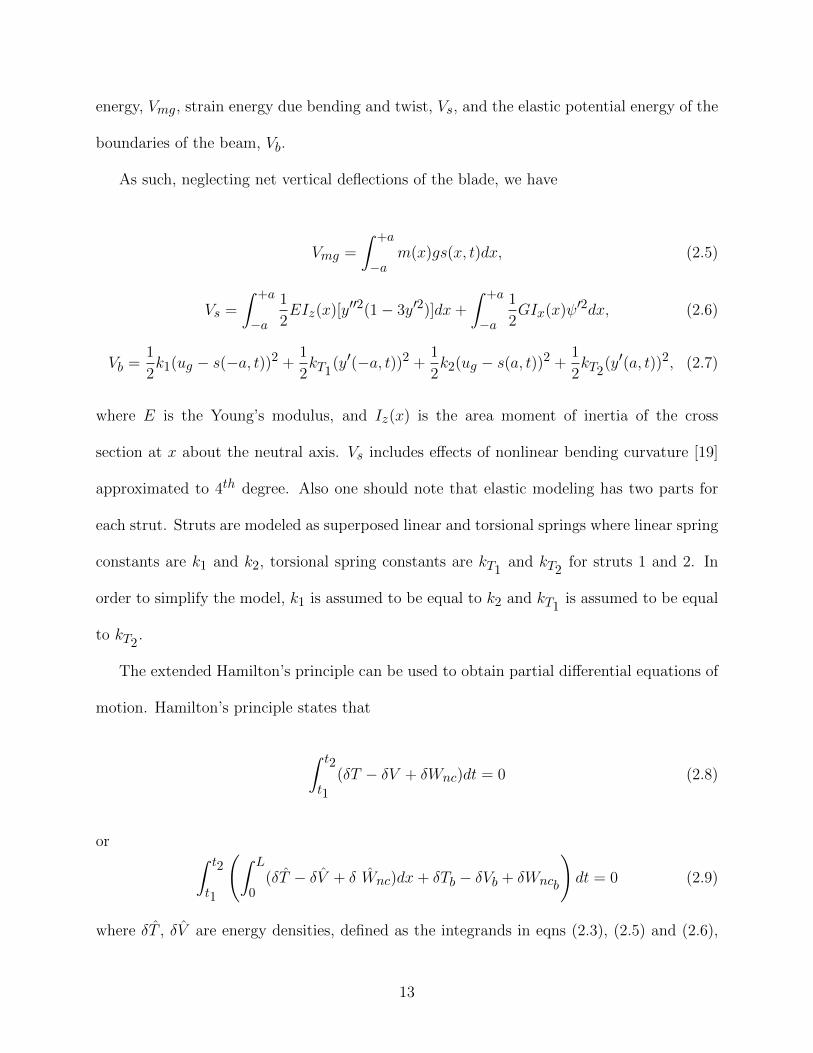
Figure 2.2 Top view representation of transverse deflection on top and twist on bottom.

ψ(x, t) ∼=Nt∑i=1

bi(t)ρi(x) (2.13)

where Nb and Nt are the numbers of bend and twist assumed modes. We will use one

assumed mode for both, so will have

y(x, t) ≈ q(t)ξ(x) (2.14)

ψ(x, t) ≈ b(t)ρ(x) (2.15)

As such, y(x, t) ≈ q(t)ξ(x), ψ(x, t) ≈ b(t)ρ(x), y′(x, t) ≈ q(t)ξ′(x), ψ′(x, t) ≈ b(t)ρ′(x).

Next we can express our energy functions

T (q, q, b, b, t) =

∫ +a

−a

1

2m(x)

((−s)2 +

(q(t)ξ(x)

)2 + (Ω(y(x, t) +R))2

)dx

+

∫ +a

−a

1

2Jxx(x)

(b(t)ρ(x) + Ω

)2+

1

2I0θ

2,

(2.16)

15

Vmg(q, q, t) =

∫ +a

−am(x)gs(q, q, t)dx, (2.17)

Vs(q, q, b, b, t) =

∫ +a

−a

1

2EI(x)

[(q(t)ξ′′(x)

)2 (1− 3

(q(t)ξ′(x)

)2)]dx

+

∫ +a

−a

1

2GJxx(x)

(b′(t)ρ(x)

)2dx,

(2.18)

Vb(q, q, b, b, t) =1

2k1(ug − s(−a, t)

)2+

1

2kT1

(q′(t)ξ(−a)

)2+

1

2k2(ug − s(a, t)

)2+

1

2kT2

(q′(t)ξ(a)

)2 (2.19)

Now, the energy equations on assumed modes can be plugged into Lagrange’s equation:

∂

∂t(∂T

∂qk)− ∂T

∂qk+∂V

∂qk= Qk (2.20)

to obtain equations of motion. Here T stands for the kinetic energy, V stands for the potential

energy, and qk is the generalized coordinate (dependent variable) from k = 1, 2..., n. Qk is

the generalized force term, and

δWnc =n∑k=1

Qkδqk (2.21)

Applying eqns. (2.14) and (2.15) for the case of a two assumed mode model

δWnc = Qqδq +Qbδb (2.22)

16

In our case of bend and twist deflections, application of Lagrange’s equations leads to

2qq

∫ a

−am(x)

[∫ x

0(ξ′)2dx

]dx+ q2q

∫ a

−am(x)

[∫ x

0(ξ′)2dx

]dx+ q

∫ a

−am(x)ξ2dx

−qq2∫ a

−am(x)

[∫ x

0(ξ′)2dx

]dx− q

∫ a

−am(x)Ω2ξ2dx−

∫ a

−am(x)Ω2Rξdx

+q

∫ a

−agm(x)

[∫ a

0(ξ′)2dx

]dx+ q3

∫ a

−agm(x)

2

[∫ x

0(ξ′)4dx

]dx+

q

∫ a

−aEI(x)ξ′′2dx− q3

∫ a

−a6EI(x)ξ′′2ξ′2

+q3k1 + k2

2

[∫ ±a0

(ξ′)2]2

+ q(kT1+ kT2

)(ξ′|±a)2 = Qq

(2.23)

b

∫ a

−aIxxρ

2dx+ b

∫ a

−aJxxGρ

′2dx = Qb (2.24)

where Qq and Qb are non-conservative aeroelastic forces to be determined in the next section.

2.3 Aeroelastic Modeling

One of the main problems with VAWTs that requires further investigation is the cyclic forces

acting on the blades. Under a constant rotation rate of the rotor and blades, the relative

velocity and angle of the wind particles hitting the blade is changing periodically, which

creates cyclic lift and drag forces and moments on the blade. These forces are associated

with the nonconservative work, Wnc, in the Hamilton’s principle (2.8).

In order to simplify our aeroelastic model, our assumption is a flow field with constant

direction and velocity. This assumption also neglects the effects of the blades on the fluid

particles. Yet one should note that blades also have their own velocity due to rotation

and deflection. Therefore the relative wind speed has a cyclic and displacement dependent

behavior.

17

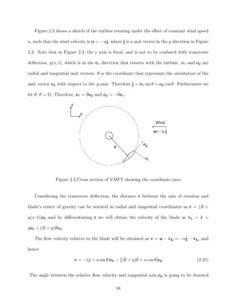
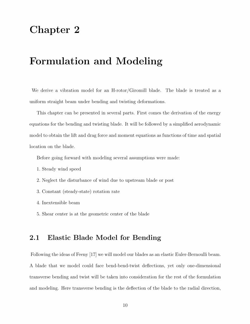
Figure 2.3 shows a sketch of the turbine rotating under the effect of constant wind speed

u, such that the wind velocity is u = −uj, where j is a unit vector in the y direction in Figure

2.3. Note that in Figure 2.3, the y axis is fixed, and is not to be confused with transverse

deflection, y(x, t), which is in the er direction that rotates with the turbine. er and eθ are

radial and tangential unit vectors. θ is the coordinate that represents the orientation of the

unit vector eθ with respect to the y-axis. Therefore j = er sin θ + eθ cos θ. Furthermore we

let θ, θ = Ω. Therefore, er = θeθ and eθ = −θer.

Figure 2.3 Cross section of VAWT showing the coordinate axes

Considering the transverse deflection, the distance r between the axis of rotation and

blade’s center of gravity can be notated in radial and tangential coordinates as r = (R +

y(x, t))er and by differentiating r we will obtain the velocity of the blade as vb = r =

yer + (R + y)θeθ.

The flow velocity relative to the blade will be obtained as v = u− vb = −uj− vb, and

hence

v = −(y + u sin θ)er − [(R + y)θ + u cos θ]eθ (2.25)

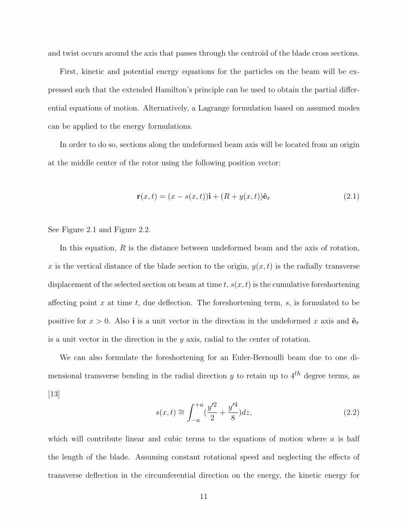
The angle between the relative flow velocity and tangential axis eθ is going to be denoted

18

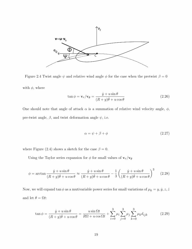
Figure 2.4 Twist angle ψ and relative wind angle φ for the case when the pretwist β = 0

with φ, where

tanφ = vr/vθ =y + u sin θ

(R + y)θ + u cos θ(2.26)

One should note that angle of attack α is a summation of relative wind velocity angle, φ,

pre-twist angle, β, and twist deformation angle ψ, i.e.

α = ψ + β + φ (2.27)

where Figure (2.4) shows a sketch for the case β = 0.

Using the Taylor series expansion for φ for small values of vr/vθ

φ = arctany + u sin θ

(R + y)θ + u cos θ≈ y + u sin θ

(R + y)θ + u cos θ− 1

3

(y + u sin θ

(R + y)θ + u cos θ

)3

(2.28)

Now, we will expand tanφ as a mutivariable power series for small variations of µk = y, y, z, z

and let θ = Ωt:

tanφ =y + u sin θ

(R + y)θ + u cos θ=

u sin Ωt

RΩ + u cos Ωt+

3∑i=0

µi

3∑j=0

µj

3∑k=0

µkdijk (2.29)

19

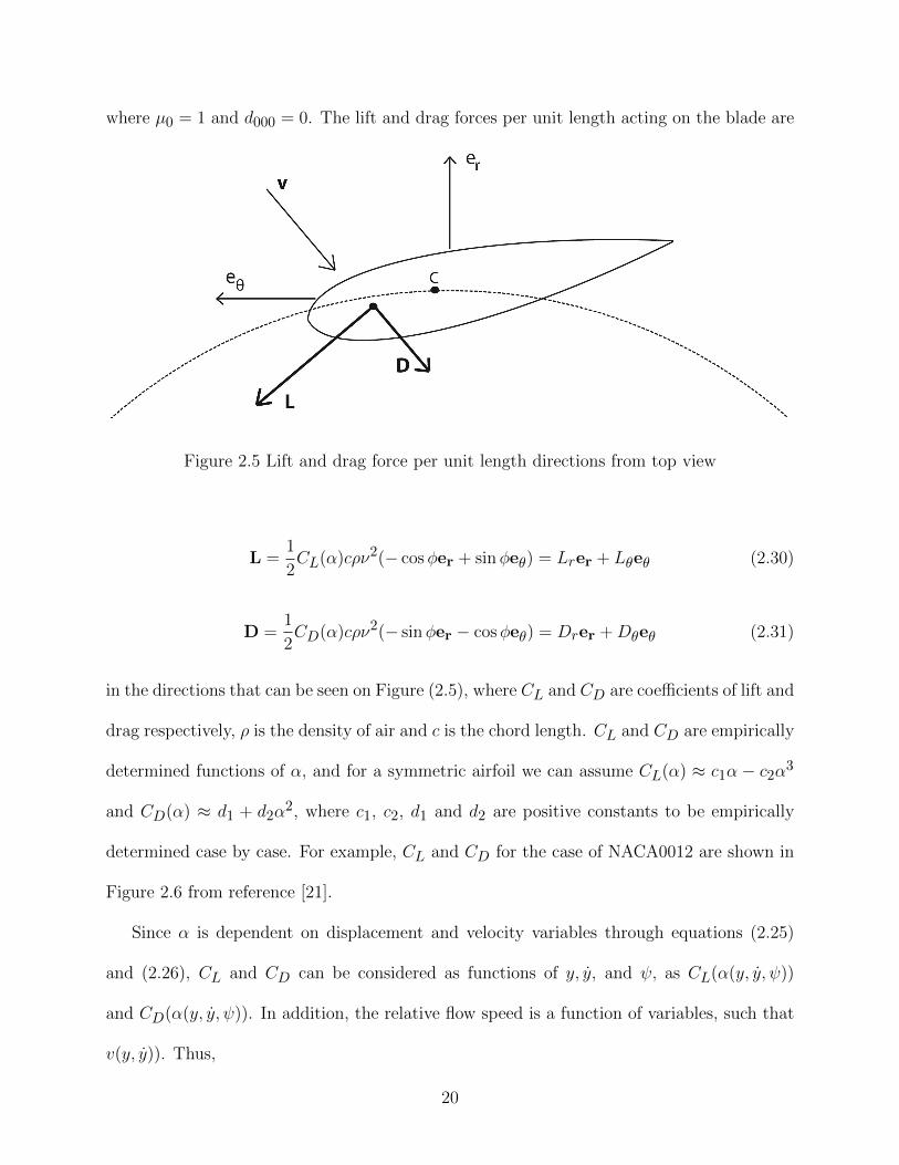
where µ0 = 1 and d000 = 0. The lift and drag forces per unit length acting on the blade are

Figure 2.5 Lift and drag force per unit length directions from top view

L =1

2CL(α)cρν2(− cosφer + sinφeθ) = Lrer + Lθeθ (2.30)

D =1

2CD(α)cρν2(− sinφer − cosφeθ) = Drer +Dθeθ (2.31)

in the directions that can be seen on Figure (2.5), where CL and CD are coefficients of lift and

drag respectively, ρ is the density of air and c is the chord length. CL and CD are empirically

determined functions of α, and for a symmetric airfoil we can assume CL(α) ≈ c1α − c2α3

and CD(α) ≈ d1 + d2α2, where c1, c2, d1 and d2 are positive constants to be empirically

determined case by case. For example, CL and CD for the case of NACA0012 are shown in

Figure 2.6 from reference [21].

Since α is dependent on displacement and velocity variables through equations (2.25)

and (2.26), CL and CD can be considered as functions of y, y, and ψ, as CL(α(y, y, ψ))

and CD(α(y, y, ψ)). In addition, the relative flow speed is a function of variables, such that

v(y, y)). Thus,

20

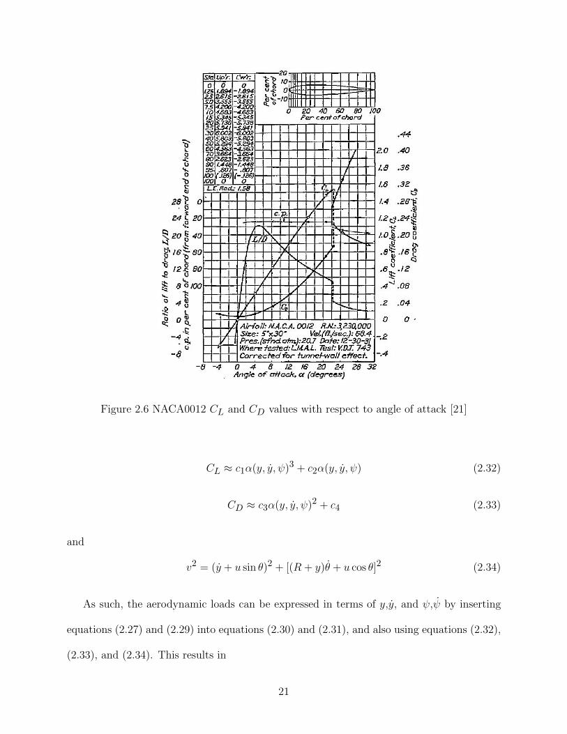
Figure 2.6 NACA0012 CL and CD values with respect to angle of attack [21]

CL ≈ c1α(y, y, ψ)3 + c2α(y, y, ψ) (2.32)

CD ≈ c3α(y, y, ψ)2 + c4 (2.33)

and

v2 = (y + u sin θ)2 + [(R + y)θ + u cos θ]2 (2.34)

As such, the aerodynamic loads can be expressed in terms of y,y, and ψ,ψ by inserting

equations (2.27) and (2.29) into equations (2.30) and (2.31), and also using equations (2.32),

(2.33), and (2.34). This results in

21

L ≈ Lr(y, y, ψ)er + Lθ(y, y, ψ)eθ (2.35)

D ≈ Dr(y, y, ψ)er +Dθ(y, y, ψ)eθ (2.36)

In our case of transverse deflection and twist, the lift and drag forces and moments

contribute to the δWnc term in equation (2.10) such that

δWnc = f(y, y, ψ, ψ, t)δy + M(y, y, ψ, ψ, t)δψ (2.37)

where radial forces will define function f such as

f(y, y, ψ, t) = Lr(y, y, ψ, t) +Dr(y, y, ψ, t) (2.38)

and a lift moment function M as

M(y, y, ψ, t) = (L cosα +D sinα) lc (2.39)

where lc is the distance between the aerodynamic center of the airfoil and its center of gravity.

One will find that lift and drag are cyclic functions, and are time periodic in the case

where Ω is constant. We will use the multi-variable Taylor series expansion (Appendix) up

to cubic terms on our functions f(y, y, ψ, t) and M(y, y, ψ, t) around (y,y,ψ)=(0,0,0). As

22

such,

f(y, y, ψ, t) = f000 + f100y + f010y + f001ψ + f200y2 + f020y

2 + f002ψ2

+f110yy + f101yψ + f011yψ + f300y3 + f030y

3 + f003ψ3

+f210y2y + f201y

2ψ + f021y2ψ + f120yy

2

+f102yψ2 + f012yψ

2 + f111yyψ

(2.40)

M(y, y, ψ, t) = M000 + M100y + M010y + M001ψ + M200y2 + M020y

2 + M002ψ2

+M110yy + M101yψ + M011yψ + M300y3 + M030y

3 + M003ψ3

+M210y2y + M201y

2ψ + M021y2ψ + M120yy

2

+M102yψ2 + M012yψ

2 + M111yyψ

(2.41)

where the coefficients fijk and Mijk are time periodic. Then we will substitute y =

q(t)ξ(x) and ψ = b(t)ρ(x) to write f(y(q, ξ(x)), y(q, ξ(x)), ψ(b, ρ(x)), t) = f(q, q, b, t;x) and

M(y(q, ξ(x)), y(q, ξ(x)), ψ(b, ρ(x)), t) = M(q, q, b, t;x), and integrate according to equation

(2.10) to write

∫ a

−af(q, q, b, t;x)ξ(x)dx = f000 + f100q + f010q + f001b+ f200q

2 + f020q2 + f002b

2

+f110qq + f101qb+ f011qb+ f300q3 + f030q

3 + f003b3

+f210q2q + f201q

2b+ f021q2b+ f120qq

2

+f102qb2 + f012qb

2 + f111qqb

(2.42)

23

∫ a

−aM(q, q, b, t;x)ρ(x)dx = M000 +M100q +M010q +M001b+M200q

2 +M020q2 +M002b

2

+M110qq +M101qb+M011qb+M300q3 +M030q

3 +M003b3

+M210q2q +M201q

2b+M021q2b+M120qq

2

+M102qb2 +M012qb

2 +M111qqb

(2.43)

where the coefficients fijk and Mijk are cyclic in time, and can be found in the Appendix.

Using equations (2.14) and (2.15), δy = ξ(x)δq and δψ = ρ(x)δb. Then the nonconserva-

tive work of equation (2.37) can be expressed in terms f(y(q, ξ(x)), y(q, ξ(x)), ψ(b, ρ(x)), t)

=f(q, q, b, t;x) and M(y(q, ξ(x)), y(q, ξ(x)), ψ(b, ρ(x)), t) = M(q, q, b, t;x) as

δWnc = f(y, y, ψ, ψ, t;x)ξ(x)δq +M(y, y, ψ, ψ, t;x)ρ(x)δb (2.44)

As such, considering equations (2.8) and (2.10) the generalized forces in equations (2.23)

and (2.24) have the form

Qq =

∫ a

−af(q, q, b, t;x)ξ(x)dx (2.45)

Qb =

∫ a

−aM(q, q, b, t;x)ρ(x)dx (2.46)

which are expressed in terms of the expansions in equations (2.42) and (2.43).

Next we will linearize the equations that we obtained.

24

2.4 Linearization

In order to conduct a simple initial numerical analysis and simulate our model we will

decrease the complexity of our model. In order to do so, several linearization methods were

discussed.

Since the system has periodic excitation, equilibria do not exist. If we consider find-

ing “unforced” equilibria, we can drop the direct excitation. The resulting equations are

nonlinear, with many terms, and with parametric excitation; so equilibria may not exist.

If we consider the equations when all cyclic time varying terms are omitted, the resulting

equations are still nonlinear with many terms, and so the equilibrium will be difficult to

express, and to use as a reference point. As such, we linearize about the equilibrium of the

non rotating system, which is zero. Thus, the “linearized” model we consider is obtained by

assuming y and ψ are small, hence quadratic and cubic terms in q and b and their derivatives

are dropped.

The resulting equations for small deflections of the rotating system within direct and

parametric excitations are

q + ω2qq + qa1(t) + qa2(t) + ba3(t) = a0 + f0(t) (2.47)

b+ ω2b b+ qe1(t) + qe2(t) + be3(t) = e0 + g0(t) (2.48)

where

a0 =

∫ a−a mΩ2ξRdx∫ a−a mξ2dx

25

a1(t) =−∫ a−a f100ξ

2(x)dx∫ a−a mξ2dx

a2(t) =−∫ a−a f010ξ

2(x)dx∫ a−a mξ2dx

a3(t) =−∫ a−a f001ξ(x)ρ(x)∫ a−a mξ2dx

f0(t) =

∫ a−a f000ξ(x)dx∫ a−a mξ2dx

ω2q =

−∫ a−a mΩ2ξ2dx+

∫ a−a gm

(∫ x0 ξ′2dx

)dx+

∫ a−a EIξ

′′2dx+kT

[(ξ′|−a)2+(ξ′|a)2

]∫ a−a mξ2dx

and,

e0 = 0

e1(t) =−∫ a−aM100ξ

2(x)dx∫ a−a Jxxρ2dx

e2(t) =−∫ a−aM010ξ

2(x)dx∫ a−a Jxxρ2dx

e3(t) =−∫ a−aM001ξ(x)ρ(x)∫ a−a Jxx

g0(t) =

∫ a−aM000ξ(x)dx∫ a−a Jxxρ2dx

ω2b =

∫ a−a IxxG(ρ′)2dx∫ a−a Jxxρ2dx

26

Chapter 3

Numerical Analysis and Simulation

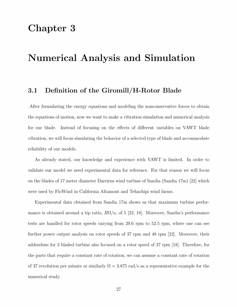
3.1 Definition of the Giromill/H-Rotor Blade

After formulating the energy equations and modeling the nonconservative forces to obtain

the equations of motion, now we want to make a vibration simulation and numerical analysis

for our blade. Instead of focusing on the effects of different variables on VAWT blade

vibration, we will focus simulating the behavior of a selected type of blade and accommodate

reliability of our models.

As already stated, our knowledge and experience with VAWT is limited. In order to

validate our model we need experimental data for reference. For that reason we will focus

on the blades of 17 meter diameter Darrieus wind turbine of Sandia (Sandia 17m) [22] which

were used by FloWind in California Altamont and Tehachipi wind farms.

Experimental data obtained from Sandia 17m shows us that maximum turbine perfor-

mance is obtained around a tip ratio, RΩ/u, of 5 [22, 18]. Moreover, Sandia’s performance

tests are handled for rotor speeds varying from 29.6 rpm to 52.5 rpm, where one can see

further power output analysis on rotor speeds of 37 rpm and 48 rpm [22]. Moreover, their

addendum for 3 bladed turbine also focused on a rotor speed of 37 rpm [18]. Therefore, for

the parts that require a constant rate of rotation, we can assume a constant rate of rotation

of 37 revolution per minute or similarly Ω = 3.875 rad/s as a representative example for the

numerical study.

27

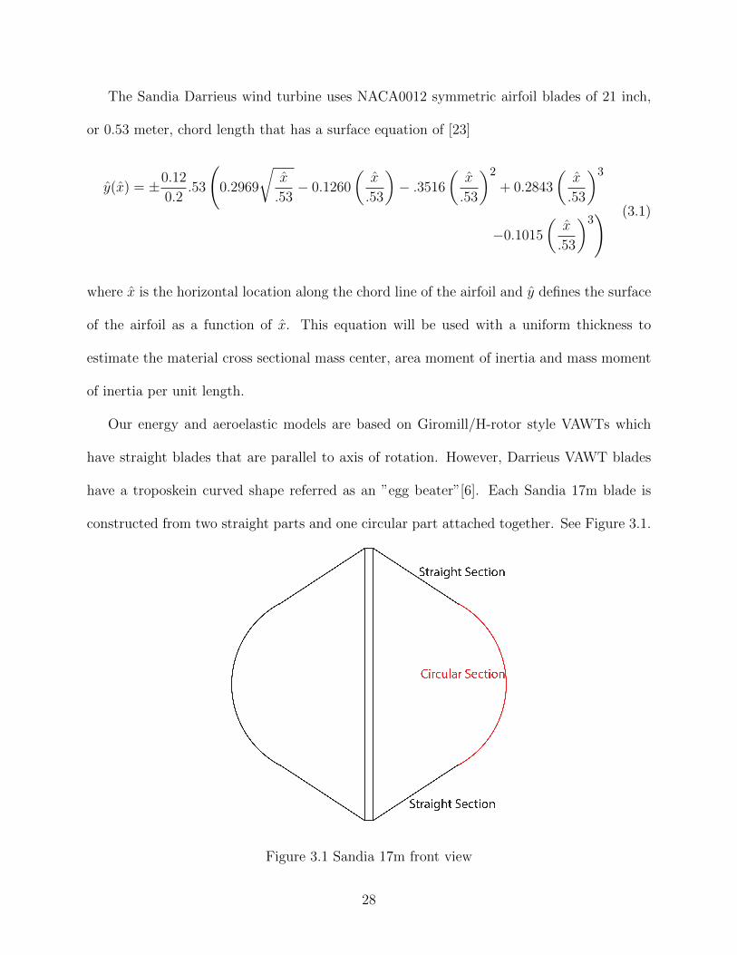
The Sandia Darrieus wind turbine uses NACA0012 symmetric airfoil blades of 21 inch,

or 0.53 meter, chord length that has a surface equation of [23]

y(x) = ±0.12

0.2.53

(0.2969

√x

.53− 0.1260

(x

.53

)− .3516

(x

.53

)2

+ 0.2843

(x

.53

)3

−0.1015

(x

.53

)3) (3.1)

where x is the horizontal location along the chord line of the airfoil and y defines the surface

of the airfoil as a function of x. This equation will be used with a uniform thickness to

estimate the material cross sectional mass center, area moment of inertia and mass moment

of inertia per unit length.

Our energy and aeroelastic models are based on Giromill/H-rotor style VAWTs which

have straight blades that are parallel to axis of rotation. However, Darrieus VAWT blades

have a troposkein curved shape referred as an ”egg beater”[6]. Each Sandia 17m blade is

constructed from two straight parts and one circular part attached together. See Figure 3.1.

Figure 3.1 Sandia 17m front view

28

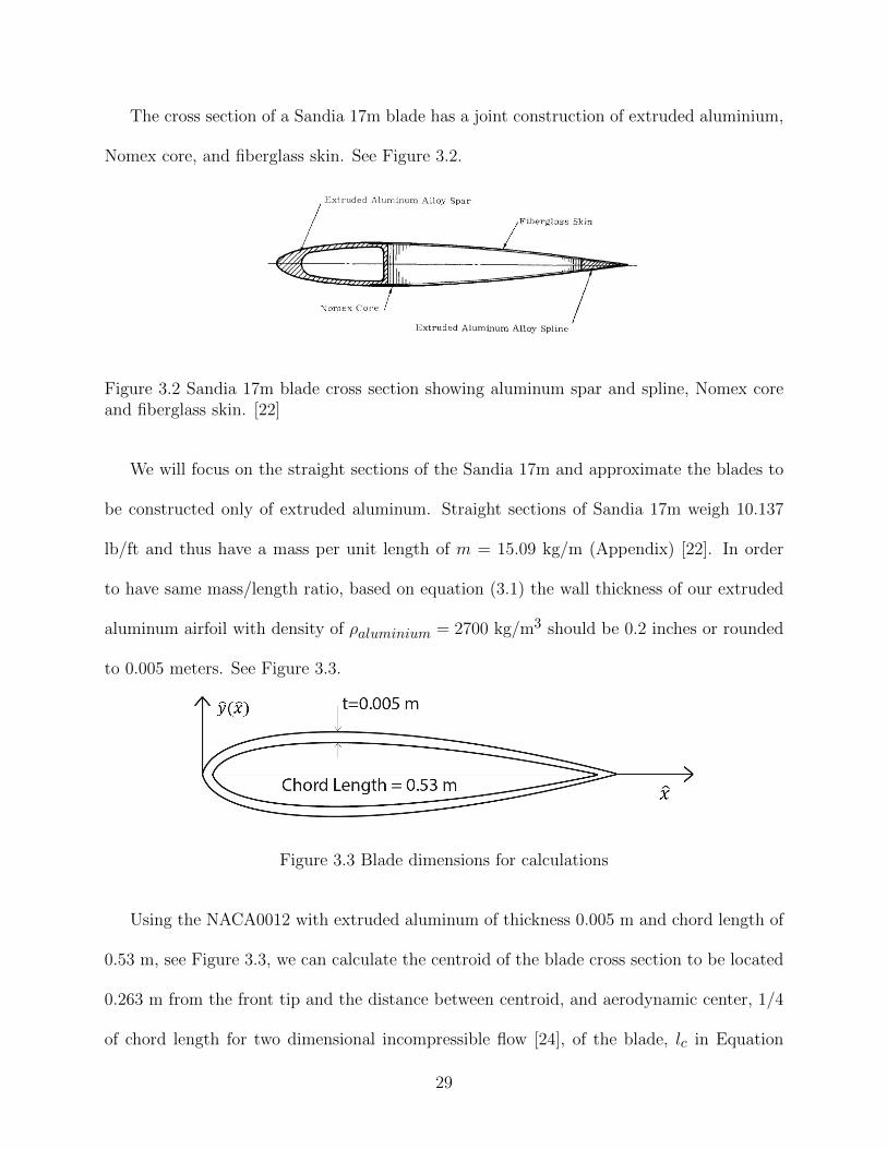
The cross section of a Sandia 17m blade has a joint construction of extruded aluminium,

Nomex core, and fiberglass skin. See Figure 3.2.

Figure 3.2 Sandia 17m blade cross section showing aluminum spar and spline, Nomex coreand fiberglass skin. [22]

We will focus on the straight sections of the Sandia 17m and approximate the blades to

be constructed only of extruded aluminum. Straight sections of Sandia 17m weigh 10.137

lb/ft and thus have a mass per unit length of m = 15.09 kg/m (Appendix) [22]. In order

to have same mass/length ratio, based on equation (3.1) the wall thickness of our extruded

aluminum airfoil with density of ρaluminium = 2700 kg/m3 should be 0.2 inches or rounded

to 0.005 meters. See Figure 3.3.

Figure 3.3 Blade dimensions for calculations

Using the NACA0012 with extruded aluminum of thickness 0.005 m and chord length of

0.53 m, see Figure 3.3, we can calculate the centroid of the blade cross section to be located

0.263 m from the front tip and the distance between centroid, and aerodynamic center, 1/4

of chord length for two dimensional incompressible flow [24], of the blade, lc in Equation

29

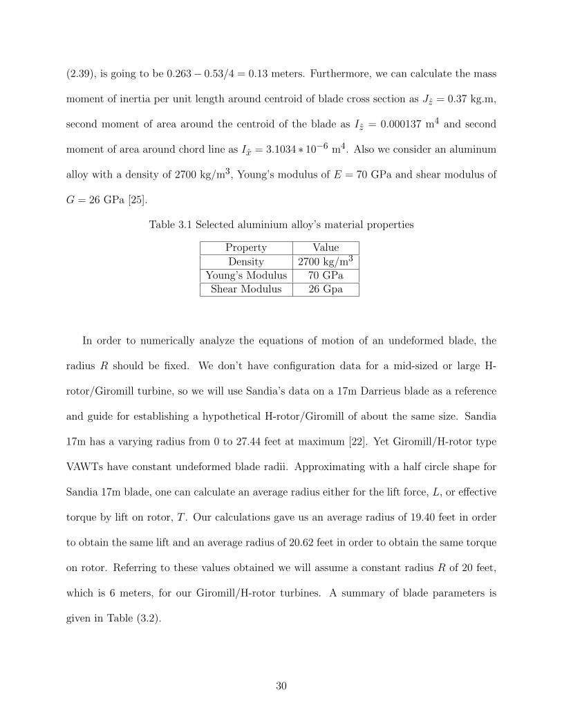
(2.39), is going to be 0.263− 0.53/4 = 0.13 meters. Furthermore, we can calculate the mass

moment of inertia per unit length around centroid of blade cross section as Jz = 0.37 kg.m,

second moment of area around the centroid of the blade as Iz = 0.000137 m4 and second

moment of area around chord line as Ix = 3.1034 ∗ 10−6 m4. Also we consider an aluminum

alloy with a density of 2700 kg/m3, Young’s modulus of E = 70 GPa and shear modulus of

G = 26 GPa [25].

Table 3.1 Selected aluminium alloy’s material properties

Property Value

Density 2700 kg/m3

Young’s Modulus 70 GPaShear Modulus 26 Gpa

In order to numerically analyze the equations of motion of an undeformed blade, the

radius R should be fixed. We don’t have configuration data for a mid-sized or large H-

rotor/Giromill turbine, so we will use Sandia’s data on a 17m Darrieus blade as a reference

and guide for establishing a hypothetical H-rotor/Giromill of about the same size. Sandia

17m has a varying radius from 0 to 27.44 feet at maximum [22]. Yet Giromill/H-rotor type

VAWTs have constant undeformed blade radii. Approximating with a half circle shape for

Sandia 17m blade, one can calculate an average radius either for the lift force, L, or effective

torque by lift on rotor, T . Our calculations gave us an average radius of 19.40 feet in order

to obtain the same lift and an average radius of 20.62 feet in order to obtain the same torque

on rotor. Referring to these values obtained we will assume a constant radius R of 20 feet,

which is 6 meters, for our Giromill/H-rotor turbines. A summary of blade parameters is

given in Table (3.2).

30

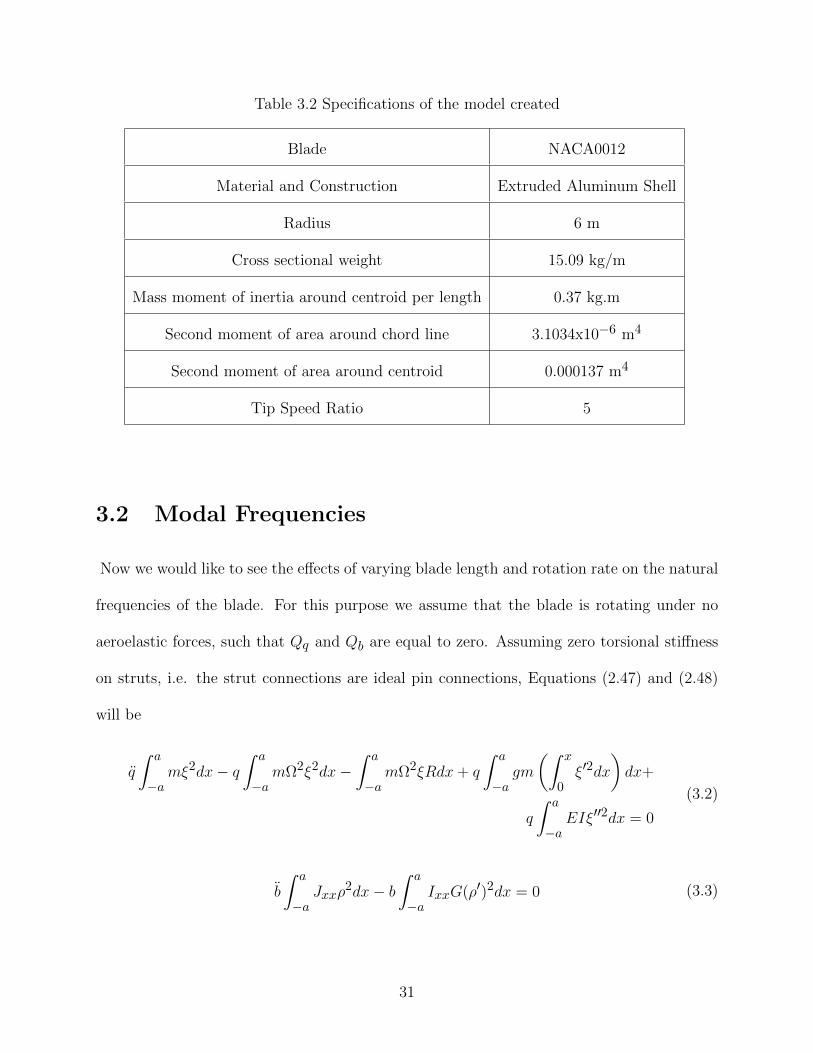
Table 3.2 Specifications of the model created

Blade NACA0012

Material and Construction Extruded Aluminum Shell

Radius 6 m

Cross sectional weight 15.09 kg/m

Mass moment of inertia around centroid per length 0.37 kg.m

Second moment of area around chord line 3.1034x10−6 m4

Second moment of area around centroid 0.000137 m4

Tip Speed Ratio 5

3.2 Modal Frequencies

Now we would like to see the effects of varying blade length and rotation rate on the natural

frequencies of the blade. For this purpose we assume that the blade is rotating under no

aeroelastic forces, such that Qq and Qb are equal to zero. Assuming zero torsional stiffness

on struts, i.e. the strut connections are ideal pin connections, Equations (2.47) and (2.48)

will be

q

∫ a

−amξ2dx− q

∫ a

−amΩ2ξ2dx−

∫ a

−amΩ2ξRdx+ q

∫ a

−agm

(∫ x

0ξ′2dx

)dx+

q

∫ a

−aEIξ′′2dx = 0

(3.2)

b

∫ a

−aJxxρ

2dx− b∫ a

−aIxxG(ρ′)2dx = 0 (3.3)

31

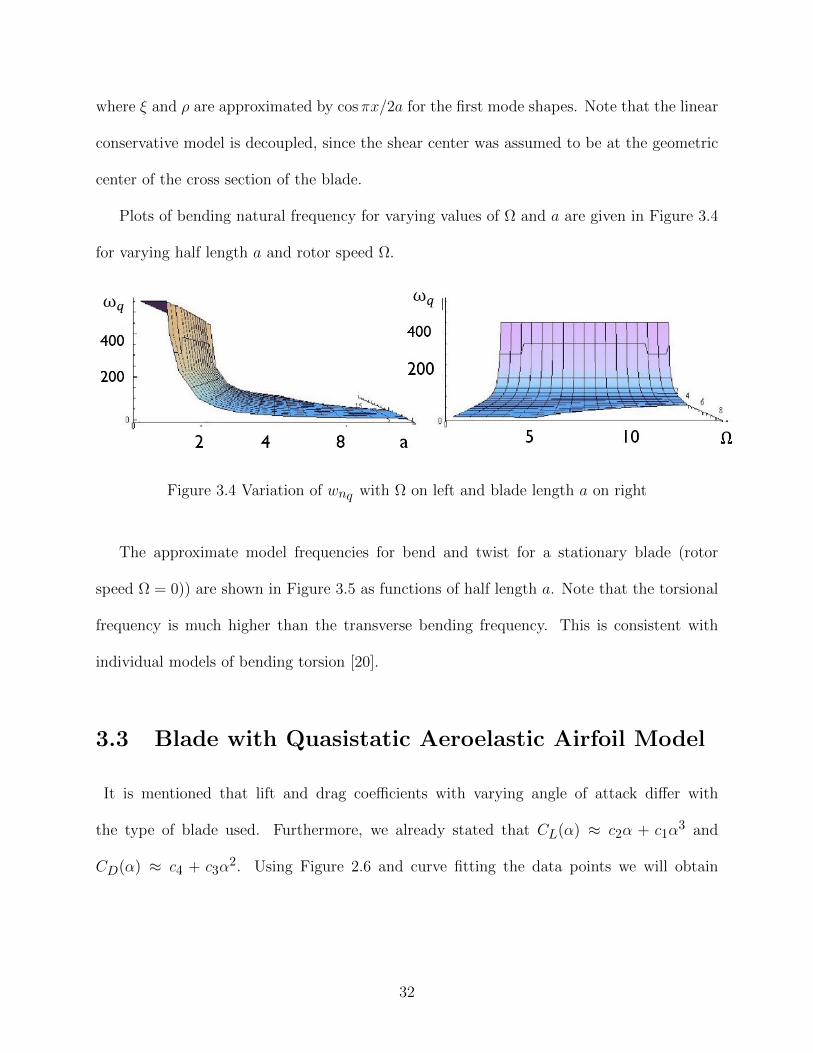
where ξ and ρ are approximated by cos πx/2a for the first mode shapes. Note that the linear

conservative model is decoupled, since the shear center was assumed to be at the geometric

center of the cross section of the blade.

Plots of bending natural frequency for varying values of Ω and a are given in Figure 3.4

for varying half length a and rotor speed Ω.

Figure 3.4 Variation of wnq with Ω on left and blade length a on right

The approximate model frequencies for bend and twist for a stationary blade (rotor

speed Ω = 0)) are shown in Figure 3.5 as functions of half length a. Note that the torsional

frequency is much higher than the transverse bending frequency. This is consistent with

individual models of bending torsion [20].

3.3 Blade with Quasistatic Aeroelastic Airfoil Model

It is mentioned that lift and drag coefficients with varying angle of attack differ with

the type of blade used. Furthermore, we already stated that CL(α) ≈ c2α + c1α3 and

CD(α) ≈ c4 + c3α2. Using Figure 2.6 and curve fitting the data points we will obtain

32

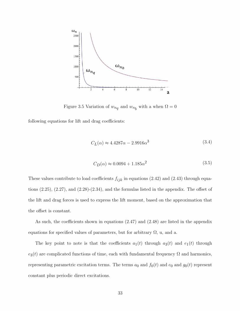
Figure 3.5 Variation of wnq and wnb with a when Ω = 0

following equations for lift and drag coefficients:

CL(α) ≈ 4.4287α− 2.9916α3 (3.4)

CD(α) ≈ 0.0094 + 1.185α2 (3.5)

These values contribute to load coefficients fijk in equations (2.42) and (2.43) through equa-

tions (2.25), (2.27), and (2.28)-(2.34), and the formulas listed in the appendix. The offset of

the lift and drag forces is used to express the lift moment, based on the approximation that

the offset is constant.

As such, the coefficients shown in equations (2.47) and (2.48) are listed in the appendix

equations for specified values of parameters, but for arbitrary Ω, u, and a.

The key point to note is that the coefficients a1(t) through a3(t) and e1(t) through

e3(t) are complicated functions of time, each with fundamental frequency Ω and harmonics,

representing parametric excitation terms. The terms a0 and f0(t) and e0 and g0(t) represent

constant plus periodic direct excitations.

33

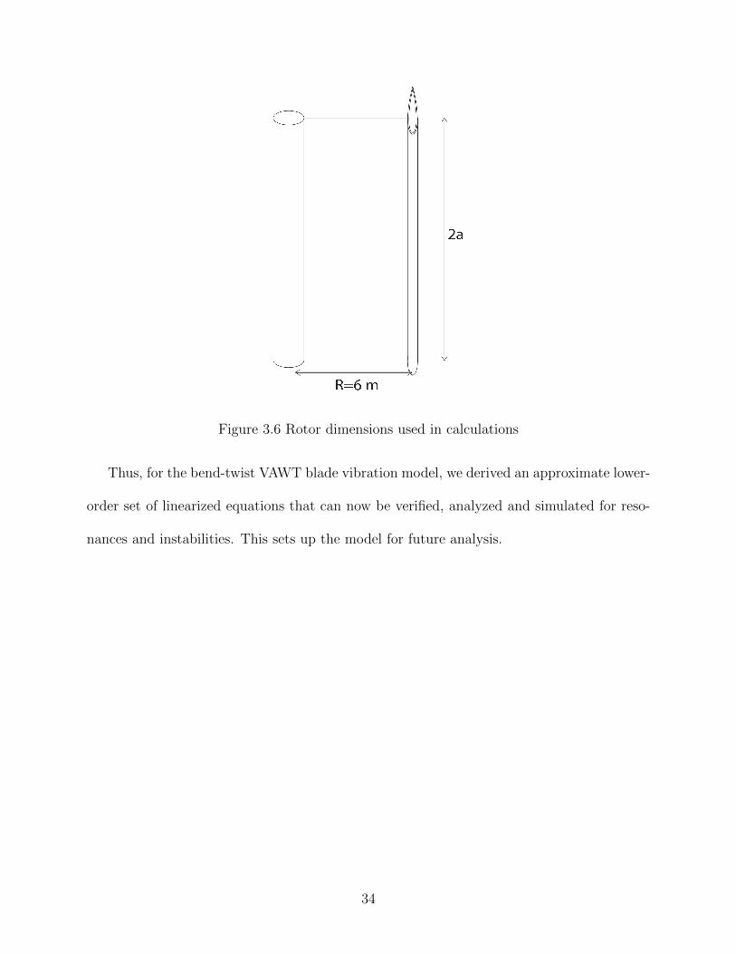
Figure 3.6 Rotor dimensions used in calculations

Thus, for the bend-twist VAWT blade vibration model, we derived an approximate lower-

order set of linearized equations that can now be verified, analyzed and simulated for reso-

nances and instabilities. This sets up the model for future analysis.

34

Chapter 4

Conclusion and Comments

4.1 Summary of Results

As a result of the research, a blade vibration model for an H-rotor/Girmoill type VAWT

for bending and twisting deflections was formulated. In addition, energy equations for an

Eulerian beam under transverse bend and twist deflections was obtained. The system was

discretized using reduced order modeling on first assumed modes on each independent vari-

able in energy equations. Lagrange’s method was applied to resulting equations to obtain

two equations of motion where generalized force terms were due aeroelastic forces on blades.

Next, an aeroelastic model was defined based on quasistatic airfoil theory. Lift and drag

forces and moments were formulated for an airfoil for changing angle of attack, where stall

effects were neglected. Resulting complicated formulas were simplified to cubic order using

Taylor series expansion. One should note that, resulting system had parametric and direct

excitation due to varying flow magnitude and direction relative to blade. Very complicated

terms were tabulated based on how to generate them with computer algebra.

In order to conduct a simple numerical analysis the system was linearized assuming small

deflections for bend and twist. Linearized equations of motion were derived for a specific

blade. Referring to Sandia 17m VAWT, hypothetical H-rotor/Giromill blade was defined

for numerical analysis where natural frequencies of the blade for a non rotating system were

found.

35

Furthermore, initial simulations showed complicated dynamics and propensity for insta-

bility.

4.2 Contribution

In a large absence of VAWT blade vibration models, this work has provided the initial steps

at modeling VAWT blade vibrations to the research literature.

The model presented here can be used as a foundation for subsequent vibration modeling

research on VAWTs. Research to be done while building this model is described in the next

section on Future Work.

4.3 Future Work

This work sets up follow-up work on a systematic study of vibrations and how responses

depend on parameters. To this end, future work will include

• verification of the terms which are very complicated

• perturbation analysis and numerical simulations to determine the potential resonances

and instabilities, and the effects of parameters on these phenomena

• higher degree of freedom reduced model, where more than one assumed mode will be

used in the calculations

• improvement of the aeroelastic model, i.e. including the effects of stall and the hys-

teretic effects caused by the influence of the changing angle of attack on the local flow

field.

36

• improvement of the structural model, for example in separating the shear center from

the geometric center, and including bend-bend-twist deflections.

• nonlinearity back into the model and perform nonlinear analyses and simulations

• modeling of the curved blades of Darrius-type turbines

37

APPENDIX

38

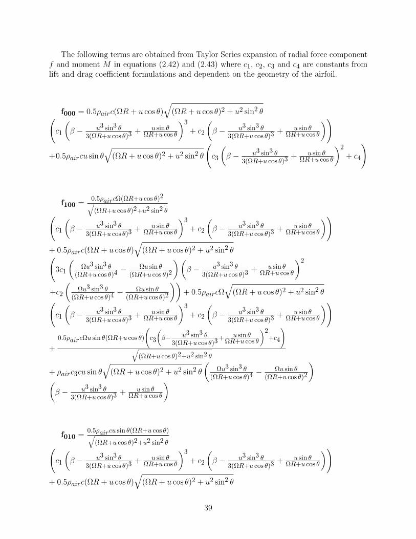
The following terms are obtained from Taylor Series expansion of radial force componentf and moment M in equations (2.42) and (2.43) where c1, c2, c3 and c4 are constants fromlift and drag coefficient formulations and dependent on the geometry of the airfoil.

f000 = 0.5ρairc(ΩR + u cos θ)√

(ΩR + u cos θ)2 + u2 sin2 θ(c1

(β − u3 sin3 θ

3(ΩR+u cos θ)3+ u sin θ

ΩR+u cos θ

)3

+ c2

(β − u3 sin3 θ


ΩR+u cos θ

))

+0.5ρaircu sin θ√

(ΩR + u cos θ)2 + u2 sin2 θ

(c3

(β − u3 sin3 θ


ΩR+u cos θ

)2

+ c4

)

f100 =0.5ρaircΩ(ΩR+u cos θ)2√(ΩR+u cos θ)2+u2 sin2 θ(

c1

(β − u3 sin3 θ


ΩR+u cos θ

)3

+ c2

(β − u3 sin3 θ


ΩR+u cos θ

))+ 0.5ρairc(ΩR + u cos θ)

√(ΩR + u cos θ)2 + u2 sin2 θ(

3c1

(Ωu3 sin3 θ

(ΩR+u cos θ)4− Ωu sin θ

(ΩR+u cos θ)2

)(β − u3 sin3 θ


ΩR+u cos θ

)2

+c2

(Ωu3 sin3 θ


(ΩR+u cos θ)2

))+ 0.5ρaircΩ


c1

(β − u3 sin3 θ


ΩR+u cos θ

)3

+ c2

(β − u3 sin3 θ


ΩR+u cos θ

))

+

0.5ρaircΩu sin θ(ΩR+u cos θ)

(c3

(β− u3 sin3 θ


ΩR+u cos θ

)2+c4

)√

(ΩR+u cos θ)2+u2 sin2 θ

+ ρairc3cu sin θ√


(Ωu3 sin3 θ


(ΩR+u cos θ)2

)(β − u3 sin3 θ


ΩR+u cos θ

)

f010 =0.5ρaircu sin θ(ΩR+u cos θ)√

(ΩR+u cos θ)2+u2 sin2 θ(c1

(β − u3 sin3 θ


ΩR+u cos θ

)3

+ c2

(β − u3 sin3 θ


ΩR+u cos θ

))+ 0.5ρairc(ΩR + u cos θ)

√(ΩR + u cos θ)2 + u2 sin2 θ

39

(3c1

(1

ΩR+u cos θ −u2 sin2 θ

(ΩR+u cos θ)3

)(β − u3 sin3 θ


ΩR+u cos θ

)2

+c2

(1


(ΩR+u cos θ)3

))

+

0.5ρaircu2 sin2 θ

(c3

(β− u3 sin3 θ


ΩR+u cos θ

)2+c4

)√


+ 0.5ρairc√


(c3

(β − u3 sin3 θ


ΩR+u cos θ

)2

+ c4

)+ ρairc3cu sin θ


(1


(ΩR+u cos θ)3

)(β − u3 sin3 θ


ΩR+u cos θ

)

f001 = 0.5ρairc(ΩR + u cos θ)√

(ΩR + u cos θ)2 + u2 sin2 θ(3c1

(β − u3 sin3 θ


ΩR+u cos θ

)2

+ c2

)+ ρairc3cu sin θ


(β − u3 sin3 θ


ΩR+u cos θ

)

f200 = 0.25ρairc4c3Ωu(ΩR+u cos θ) sin θ

(Ωu3 sin3 θ


(ΩR+u cos θ)2

)(− u3 sin3 θ


ΩR+u cos θ+β

)√


+c3u sin θ√

(ΩR + u cos θ)2 + u2 sin2 θ(2

(Ωu3 sin3 θ


(ΩR+u cos θ)2

)2

+ 2

(2Ω2u sin θ

(ΩR+u cos θ)3− 4Ω2u3 sin3 θ

(ΩR+u cos θ)5

)(− u3 sin3 θ


ΩR+u cos θ + β

))+u sin θ

Ω2√(ΩR+u cos θ)2+u2 sin2 θ

− Ω2(ΩR+u cos θ)2((ΩR+u cos θ)2+u2 sin2 θ

)3/2

(c3

(− u3 sin3 θ


ΩR+u cos θ + β

)2

+ c4

))

+ 0.5ρairc

(2

(Ω(ΩR+u cos θ)2√

(ΩR+u cos θ)2+u2 sin2 θ+ Ω


)

40

(3c1

(Ωu3 sin3 θ


(ΩR+u cos θ)2

)(− u3 sin3 θ


ΩR+u cos θ + β

)2

+c2

(Ωu3 sin3 θ


(ΩR+u cos θ)2

))+

(c1

(− u3 sin3 θ


ΩR+u cos θ + β

)3

+c2

(− u3 sin3 θ


ΩR+u cos θ + β

))(

2(ΩR+u cos θ)Ω2√(ΩR+u cos θ)2+u2 sin2 θ

+ (ΩR + u cos θ) Ω2√(ΩR+u cos θ)2+u2 sin2 θ


)3/2

+(ΩR + u cos θ)


(c2

(2Ω2u sin θ


(ΩR+u cos θ)5

)+c1

(6

(− u3 sin3 θ


ΩR+u cos θ + β

)(Ωu3 sin3 θ


(ΩR+u cos θ)2

)2

+

3

(2Ω2u sin θ


(ΩR+u cos θ)5

)(− u3 sin3 θ


ΩR+u cos θ + β

)2)))

f020 = 0.25ρairc

(4c3

(1


(ΩR+u cos θ)3

)(− u3 sin3 θ


ΩR+u cos θ + β

)(

u2 sin2 θ√(ΩR+u cos θ)2+u2 sin2 θ

+√


)

+c3u sin θ√


(2

(1


(ΩR+u cos θ)3

)2

−4u sin θ

(− u3 sin3 θ


ΩR+u cos θ+β

)(ΩR+u cos θ)3

+

(c3

(− u3 sin3 θ


ΩR+u cos θ + β

)2

+c4)u 1√

(ΩR+u cos θ)2+u2 sin2 θ− u2 sin2 θ(

(ΩR+u cos θ)2+u2 sin2 θ)3/2

sin θ

+ 2u sin θ√(ΩR+u cos θ)2+u2 sin2 θ

))

+ 0.5ρairc

(2u(ΩR+u cos θ) sin θ√


41

((3c1

(1


(ΩR+u cos θ)3

)(− u3 sin3 θ


ΩR+u cos θ + β

)2

+c2

(1


(ΩR+u cos θ)3

)))+(ΩR + u cos θ)

1√(ΩR+u cos θ)2+u2 sin2 θ

− u2 sin2 θ((ΩR+u cos θ)2+u2 sin2 θ

)3/2

(c1

(− u3 sin3 θ


ΩR+u cos θ + β

)3

+ c2

(− u3 sin3 θ


ΩR+u cos θ + β

))

+(ΩR + u cos θ)√


(c1

(6

(1


(ΩR+u cos θ)3

)2

(− u3 sin3 θ


ΩR+u cos θ + β

)−

6u sin θ

(− u3 sin3 θ


ΩR+u cos θ+β

)2

(ΩR+u cos θ)3

− 2c2u sin θ

(ΩR+u cos θ)3

))

f002 = 0.5

(3.ρairc1c(ΩR + u cos θ)


β − u3 sin3 θ3(ΩR+u cos θ)3

+ u sin θΩR+u cos θ

)+ρairc3cu sin θ

√(ΩR + u cos θ)2 + u2 sin2 θ + 0.

)

f110 =0.5ρaircΩ√


(3c1

(1


(ΩR+u cos θ)3

)(− u3 sin3 θ


ΩR+u cos θ + β

)2

+ c2

(1


(ΩR+u cos θ)3

))(ΩR + u cos θ)2

− 0.5ρaircΩu sin θ((ΩR+u cos θ)2+u2 sin2 θ

)3/2(c1

(− u3 sin3 θ


ΩR+u cos θ + β

)3

+ c2

(− u3 sin3 θ


ΩR+u cos θ + β

))(ΩR + u cos θ)2

+ρairc3cΩu sin θ

(1

ΩR+u cos θ− u2 sin2 θ

(ΩR+u cos θ)3

)(− u3 sin3 θ


ΩR+u cos θ+β

)(ΩR+u cos θ)√


42

+

0.5ρaircΩ

(c3

(− u3 sin3 θ


ΩR+u cos θ+β

)2+c4

)(ΩR+u cos θ)√


−0.5ρaircΩu

2 sin2 θ

(c3

(− u3 sin3 θ


ΩR+u cos θ+β

)2+c4

)(ΩR+u cos θ)(


+ 0.5ρairc√


(3c1

(3Ωu2 sin2 θ

(ΩR+u cos θ)4− Ω

(ΩR+u cos θ)2

)(− u3 sin3 θ


ΩR+u cos θ + β

)2

+6c1

(1


(ΩR+u cos θ)3

)(Ωu3 sin3 θ


(ΩR+u cos θ)2

)(− u3 sin3 θ


ΩR+u cos θ + β

)+c2

(3Ωu2 sin2 θ


(ΩR+u cos θ)2

))(ΩR + u cos θ)

+0.5ρaircu sin θ√


(3c1

(Ωu3 sin3 θ


(ΩR+u cos θ)2

)(− u3 sin3 θ


ΩR+u cos θ + β

)2

+c2

(Ωu3 sin3 θ


(ΩR+u cos θ)2

))(ΩR + u cos θ)



(1


(ΩR+u cos θ)3

)(

Ωu3 sin3 θ(ΩR+u cos θ)4

− Ωu sin θ(ΩR+u cos θ)2

)+ ρairc3cu sin θ


(3Ωu2 sin2 θ


(ΩR+u cos θ)2

)(− u3 sin3 θ


ΩR+u cos θ + β

)+ ρairc3c




)(− u3 sin3 θ


ΩR+u cos θ + β

)

+ρairc3cu

2 sin2 θ

(Ωu3 sin3 θ


(ΩR+u cos θ)2

)(− u3 sin3 θ


ΩR+u cos θ+β

)√


+ 0.5ρaircΩ√


(3c1

(1


(ΩR+u cos θ)3

)(− u3 sin3 θ


ΩR+u cos θ + β

)2

+ c2

(1


(ΩR+u cos θ)3

))

43

+

0.5ρaircΩu sin θ

(c1

(− u3 sin3 θ


ΩR+u cos θ+β

)3+c2

(− u3 sin3 θ


ΩR+u cos θ+β

))√


f101 =

0.5ρaircΩ(ΩR+u cos θ)2

(3c1

(β− u3 sin3 θ


ΩR+u cos θ

)2+c2

)√


+ 0.5ρaircΩ√


(3c1

(β − u3 sin3 θ


ΩR+u cos θ

)2

+ c2

)+ 3.ρairc1c(ΩR + u cos θ)


(Ωu3 sin3 θ


(ΩR+u cos θ)2

)(β − u3 sin3 θ


ΩR+u cos θ

)

+ρairc3cΩu sin θ(ΩR+u cos θ)

(β− u3 sin3 θ


ΩR+u cos θ

)√




(Ωu3 sin3 θ


(ΩR+u cos θ)2

)

f011 =

0.5ρaircu sin θ(ΩR+u cos θ)

(3c1

(β− u3 sin3 θ


ΩR+u cos θ

)2+c2

)√


+ 3.ρairc1c(ΩR + u cos θ)√


(1


(ΩR+u cos θ)3

)(β − u3 sin3 θ


ΩR+u cos θ

)+ρairc3cu

2 sin2 θ

(β− u3 sin3 θ


ΩR+u cos θ

)√


+ ρairc3c√


(β − u3 sin3 θ


ΩR+u cos θ

)+ ρairc3cu sin θ


(1


(ΩR+u cos θ)3

)

f300 = 16

(0.5ρairc

(6c3u sin θ

(Ωu3 sin3 θ


(ΩR+u cos θ)2

)(− u3 sin3 θ


ΩR+u cos θ + β

)

44



)3/2

+c3u sin θ


6

(2Ω2u sin θ


(ΩR+u cos θ)5

)(Ωu3 sin3 θ


(ΩR+u cos θ)2

)+2

(20Ω3u3 sin3 θ(ΩR+u cos θ)6

− 6Ω3u sin θ(ΩR+u cos θ)4

)(− u3 sin3 θ


ΩR+u cos θ + β

))+

3c3Ωu(ΩR+u cos θ) sin θ√(ΩR+u cos θ)2+u2 sin2 θ(

2

(Ωu3 sin3 θ


(ΩR+u cos θ)2

)2

+ 2

(2Ω2u sin θ


(ΩR+u cos θ)5

)(− u3 sin3 θ


ΩR+u cos θ + β

))+u sin θ

3Ω3(ΩR+u cos θ)3((ΩR+u cos θ)2+u2 sin2 θ

)5/2− 3Ω3(ΩR+u cos θ)(


(c3

(− u3 sin3 θ


ΩR+u cos θ + β

)2

+ c4

))

+0.5ρairc

((c1

(− u3 sin3 θ


ΩR+u cos θ + β

)3

+c2

(− u3 sin3 θ


ΩR+u cos θ + β

))(ΩR + u cos θ)

3Ω3(ΩR+u cos θ)3((ΩR+u cos θ)2+u2 sin2 θ

)5/2− 3Ω3(ΩR+u cos θ)(


+3Ω



)3/2

+3

(3c1

(Ωu3 sin3 θ


(ΩR+u cos θ)2

)(− u3 sin3 θ


ΩR+u cos θ + β

)2

+c2

(Ωu3 sin3 θ


(ΩR+u cos θ)2

))(2(ΩR+u cos θ)Ω2√

(ΩR+u cos θ)2+u2 sin2 θ+ (ΩR + u cos θ) Ω2√

(ΩR+u cos θ)2+u2 sin2 θ− Ω2(ΩR+u cos θ)2(


+(ΩR + u cos θ)


(c2



)+c1

(6

(Ωu3 sin3 θ


(ΩR+u cos θ)2

)3

+ 18

(2Ω2u sin θ


(ΩR+u cos θ)5

)

45

(− u3 sin3 θ


ΩR+u cos θ + β

)(Ωu3 sin3 θ


(ΩR+u cos θ)2

)+3



)(− u3 sin3 θ


ΩR+u cos θ + β

)2))

+3




)(c2

(2Ω2u sin θ


(ΩR+u cos θ)5

)+c1

(6

(− u3 sin3 θ


ΩR+u cos θ + β

)(Ωu3 sin3 θ


(ΩR+u cos θ)2

)2

+3

(2Ω2u sin θ


(ΩR+u cos θ)5

)(− u3 sin3 θ


ΩR+u cos θ + β

)2))))

f030 = 16

(0.5ρairc

(c3u sin θ

√(ΩR + u cos θ)2 + u2 sin2 θ−12u sin θ

(1


(ΩR+u cos θ)3

)(ΩR+u cos θ)3

−4

(− u3 sin3 θ


ΩR+u cos θ+β

)(ΩR+u cos θ)3

+3c3

(u2 sin2 θ√

(ΩR+u cos θ)2+u2 sin2 θ+√


)2

(1


(ΩR+u cos θ)3

)2

−4u sin θ

(− u3 sin3 θ


ΩR+u cos θ+β

)(ΩR+u cos θ)3

+

(c3

(− u3 sin3 θ


ΩR+u cos θ + β

)2

+ c4

)(u sin θ 3u3 sin3 θ(


− 3u sin θ((ΩR+u cos θ)2+u2 sin2 θ

)3/2

+3



)3/2

+6c3

(1


(ΩR+u cos θ)3

)(− u3 sin3 θ


ΩR+u cos θ + β

)u



)3/2

sin θ+

2u sin θ√(ΩR+u cos θ)2+u2 sin2 θ

))+ 0.5ρairc (3(ΩR + u cos θ)

46



)3/2

(

3c1

(1


(ΩR+u cos θ)3

)(− u3 sin3 θ


ΩR+u cos θ + β

)2

+ c2

(1


(ΩR+u cos θ)3

))+(ΩR + u cos θ) 3u3 sin3 θ(


− 3u sin θ((ΩR+u cos θ)2+u2 sin2 θ

)3/2

(c1

(− u3 sin3 θ


ΩR+u cos θ + β

)3

+c2

(− u3 sin3 θ


ΩR+u cos θ + β

))+ (ΩR + u cos θ)


c1

(6

(1


(ΩR+u cos θ)3

)3

− 36u sin θ(ΩR+u cos θ)3

(− u3 sin3 θ


ΩR+u cos θ + β

)(

1ΩR+u cos θ −

u2 sin2 θ(ΩR+u cos θ)3

)−

6

(− u3 sin3 θ


ΩR+u cos θ+β

)2

(ΩR+u cos θ)3

− 2c2(ΩR+u cos θ)3

+

3u(ΩR+u cos θ) sin θ√(ΩR+u cos θ)2+u2 sin2 θ

(c1

(6

(1


(ΩR+u cos θ)3

)2

(− u3 sin3 θ


ΩR+u cos θ + β

)

−6u sin θ

(− u3 sin3 θ


ΩR+u cos θ+β

)2

(ΩR+u cos θ)3

− 2c2u sin θ

(ΩR+u cos θ)3

f003 = 12

0.5ρairc

− 4c3Ωu2(ΩR+u cos θ)((ΩR+u cos θ)2+u2 sin2 θ

)3/2

(Ωu3 sin3 θ


(ΩR+u cos θ)2

)(− u3 sin3 θ


ΩR+u cos θ + β

)sin2 θ + 1√

(ΩR+u cos θ)2+u2 sin2 θ(c3u

2

(2

(Ωu3 sin3 θ


(ΩR+u cos θ)2

)2

+ 2

(2Ω2u sin θ


(ΩR+u cos θ)5

)(− u3 sin3 θ


ΩR+u cos θ + β

))sin2 θ

)+

47

4c3Ωu(ΩR+u cos θ)

(1


(ΩR+u cos θ)3

)(Ωu3 sin3 θ


(ΩR+u cos θ)2

)sin θ√


+4c3Ωu(ΩR+u cos θ)

(3Ωu2 sin2 θ


(ΩR+u cos θ)2

)(− u3 sin3 θ


ΩR+u cos θ+β

)sin θ√


+2c3u

(1


(ΩR+u cos θ)3

)(− u3 sin3 θ


ΩR+u cos θ + β

) Ω2√



sin θ

+c3u√


(2

(1


(ΩR+u cos θ)3

)(

2Ω2u sin θ(ΩR+u cos θ)3

− 4Ω2u3 sin3 θ(ΩR+u cos θ)5

)+ 4

(3Ωu2 sin2 θ


(ΩR+u cos θ)2

)(



)+ 2

(2Ω2


(ΩR+u cos θ)5

)(− u3 sin3 θ


ΩR+u cos θ + β

))sin θ

+u

3Ω2u(ΩR+u cos θ)2 sin θ((ΩR+u cos θ)2+u2 sin2 θ

)5/2− Ω2u sin θ(


(c3

(− u3 sin3 θ


ΩR+u cos θ + β

)2

+ c4

)sin θ

+4c3Ω(ΩR+u cos θ)

(Ωu3 sin3 θ


(ΩR+u cos θ)2

)(− u3 sin3 θ


ΩR+u cos θ+β

)√


+c3


2

(Ωu3 sin3 θ


(ΩR+u cos θ)2

)2

+2

(2Ω2u sin θ


(ΩR+u cos θ)5

)(− u3 sin3 θ


ΩR+u cos θ + β

))+



)3/2

(c3

(− u3 sin3 θ


ΩR+u cos θ + β

)2

+c4)) + 0.5ρairc

(2




)

48

(3c1

(3Ωu2 sin2 θ


(ΩR+u cos θ)2

)(− u3 sin3 θ


ΩR+u cos θ + β

)2

+

6c1

(1


(ΩR+u cos θ)3

)(Ωu3 sin3 θ


(ΩR+u cos θ)2

)(− u3 sin3 θ


ΩR+u cos θ + β

)+c2

(3Ωu2 sin2 θ


(ΩR+u cos θ)2

))+2

Ωu sin θ√(ΩR+u cos θ)2+u2 sin2 θ

− Ωu(ΩR+u cos θ)2 sin θ((ΩR+u cos θ)2+u2 sin2 θ

)3/2

(

3c1

(Ωu3 sin3 θ


(ΩR+u cos θ)2

)(− u3 sin3 θ


ΩR+u cos θ + β

)2

+c2

(Ωu3 sin3 θ


(ΩR+u cos θ)2

))+

(c1

(− u3 sin3 θ


ΩR+u cos θ + β

)3

+c2

(− u3 sin3 θ


ΩR+u cos θ + β

))(ΩR + u cos θ)


)5/2

− Ω2u sin θ((ΩR+u cos θ)2+u2 sin2 θ

)3/2

− 2Ω2u(ΩR+u cos θ) sin θ((ΩR+u cos θ)2+u2 sin2 θ

)3/2

+

(3c1

(1


(ΩR+u cos θ)3

)(− u3 sin3 θ


ΩR+u cos θ + β

)2

+c2

(1


(ΩR+u cos θ)3





+ (ΩR + u cos θ)


(c2

(2Ω2


(ΩR+u cos θ)5

)+c1

(6

(1


(ΩR+u cos θ)3

)(



)2

+ 12

(3Ωu2 sin2 θ


(ΩR+u cos θ)2

)(− u3 sin3 θ


ΩR+u cos θ + β

)(Ωu3 sin3 θ


(ΩR+u cos θ)2

)+3

(2Ω2


(ΩR+u cos θ)5

)(− u3 sin3 θ


ΩR+u cos θ + β

)2

+6

(1


(ΩR+u cos θ)3

)(2Ω2u sin θ


(ΩR+u cos θ)5

)

49

(− u3 sin3 θ


ΩR+u cos θ + β

)))+ 1√

(ΩR+u cos θ)2+u2 sin2 θ(u(ΩR + u cos θ) sin θ

(c2

(2Ω2u sin θ


(ΩR+u cos θ)5

)+c1

(6

(− u3 sin3 θ


ΩR+u cos θ + β

)(Ωu3 sin3 θ


(ΩR+u cos θ)2

)2

+3

(2Ω2u sin θ


(ΩR+u cos θ)5

)(− u3 sin3 θ


ΩR+u cos θ + β

)2)))))

f210 = 12

0.5ρairc

− 4c3Ωu2(ΩR+u cos θ)((ΩR+u cos θ)2+u2 sin2 θ

)3/2(Ωu3 sin3 θ


(ΩR+u cos θ)2

)(− u3 sin3 θ


ΩR+u cos θ + β

)sin2 θc3u

22

(Ωu3 sin3 θ


(ΩR+u cos θ)2

)2

√(ΩR+u cos θ)2+u2 sin2 θ

+2

2

(2Ω2u sin θ


(ΩR+u cos θ)5

)(− u3 sin3 θ


ΩR+u cos θ+β

)sin2 θ√



(1


(ΩR+u cos θ)3

)(Ωu3 sin3 θ


(ΩR+u cos θ)2

)sin θ√



(3Ωu2 sin2 θ


(ΩR+u cos θ)2

)(− u3 sin3 θ


ΩR+u cos θ+β

)sin θ√


+2c3u

(1


(ΩR+u cos θ)3

)(− u3 sin3 θ


ΩR+u cos θ + β

) Ω2√



sin θ

+c3u√


(2

(1


(ΩR+u cos θ)3

)(



)+4

(3Ωu2 sin2 θ


(ΩR+u cos θ)2

)(Ωu3 sin3 θ


(ΩR+u cos θ)2

)

50

+2

(2Ω2


(ΩR+u cos θ)5

)(− u3 sin3 θ


ΩR+u cos θ + β

))sin θ

+u


)5/2− Ω2u sin θ(


(c3

(− u3 sin3 θ


ΩR+u cos θ + β

)2

+ c4

)sin θ

+4c3Ω(ΩR+u cos θ)

(Ωu3 sin3 θ


(ΩR+u cos θ)2

)(− u3 sin3 θ


ΩR+u cos θ+β

)√


+c3


(2

(Ωu3 sin3 θ


(ΩR+u cos θ)2

)2

+2

(2Ω2u sin θ


(ΩR+u cos θ)5

)(− u3 sin3 θ


ΩR+u cos θ + β

))+



)3/2

(c3

(− u3 sin3 θ


ΩR+u cos θ + β

)2

+c4)) + 0.5ρairc

(2




)(

3c1

(3Ωu2 sin2 θ


(ΩR+u cos θ)2

)(− u3 sin3 θ


ΩR+u cos θ + β

)2

+6c1

(1


(ΩR+u cos θ)3

)(Ωu3 sin3 θ


(ΩR+u cos θ)2

)(− u3 sin3 θ


ΩR+u cos θ + β

)+c2

(3Ωu2 sin2 θ


(ΩR+u cos θ)2

))+2

Ωu sin θ√(ΩR+u cos θ)2+u2 sin2 θ

− Ωu(ΩR+u cos θ)2 sin θ((ΩR+u cos θ)2+u2 sin2 θ

)3/2

(

3c1

(Ωu3 sin3 θ


(ΩR+u cos θ)2

)(− u3 sin3 θ


ΩR+u cos θ + β

)2

+c2

(Ωu3 sin3 θ


(ΩR+u cos θ)2

))+

(c1

(− u3 sin3 θ


ΩR+u cos θ + β

)3

+c2

(− u3 sin3 θ


ΩR+u cos θ + β

))((ΩR + u cos θ)

51


)5/2− Ω2u sin θ(


− 2Ω2u(ΩR+u cos θ) sin θ(


+

(3c1

(1


(ΩR+u cos θ)3

)(− u3 sin3 θ


ΩR+u cos θ + β

)2

+c2

(1


(ΩR+u cos θ)3





+ (ΩR + u cos θ)


(c2

(2Ω2


(ΩR+u cos θ)5

)+c1

(6

(1


(ΩR+u cos θ)3

)(



)2

+ 12

(3Ωu2 sin2 θ


(ΩR+u cos θ)2

)(− u3 sin3 θ


ΩR+u cos θ + β

)(Ωu3 sin3 θ


(ΩR+u cos θ)2

)+3

(2Ω2


(ΩR+u cos θ)5

)(− u3 sin3 θ


ΩR+u cos θ + β

)2

+ 6

(1


(ΩR+u cos θ)3

)(



)(− u3 sin3 θ


ΩR+u cos θ + β

)))+

u(ΩR+u cos θ) sin θ√(ΩR+u cos θ)2+u2 sin2 θ(

c2

(2Ω2u sin θ


(ΩR+u cos θ)5

)+ c1

(6

(− u3 sin3 θ


ΩR+u cos θ + β

)(



)2

+ 3

(2Ω2u sin θ


(ΩR+u cos θ)5

)(− u3 sin3 θ


ΩR+u cos θ + β

)2))))

52

f201 = 12

(0.5ρairc

((2Ω2(ΩR+u cos θ)√




(3c1(β − u3 sin3 θ


ΩR+u cos θ

)2

+c2) + c1(ΩR + u cos θ)√


(6

(2Ω2u sin θ


(ΩR+u cos θ)5

)(β − u3 sin3 θ


ΩR+u cos θ

)+ 6

(Ωu3 sin3 θ


(ΩR+u cos θ)2

)2)

+12c1

(Ωu3 sin3 θ


(ΩR+u cos θ)2

)(

Ω(ΩR+u cos θ)2√(ΩR+u cos θ)2+u2 sin2 θ

+ Ω√


)(β − u3 sin3 θ


ΩR+u cos θ

))+ 0.5ρairc (2c3u sin θ Ω2√



(β − u3 sin3 θ


ΩR+u cos θ

)+2c3u sin θ


(2Ω2u sin θ


(ΩR+u cos θ)5

)

+4c3Ωu sin θ(ΩR+u cos θ)

(Ωu3 sin3 θ


(ΩR+u cos θ)2

)√


f021 = 12

(0.5ρairc

((ΩR + u cos θ)

(1√



)3/2

(

3c1

(β − u3 sin3 θ


ΩR+u cos θ

)2

+ c2

)

+12c1u sin θ(ΩR+u cos θ)

(1


(ΩR+u cos θ)3

)(β− u3 sin3 θ


ΩR+u cos θ

)√


53

+c1(ΩR + u cos θ)√


(6

(1


(ΩR+u cos θ)3

)2

−

12u sin θ

(β− u3 sin3 θ


ΩR+u cos θ

)(ΩR+u cos θ)3

+0.5ρairc

(2c3

(u sin θ

(1√



)3/2

+ 2u sin θ√(ΩR+u cos θ)2+u2 sin2 θ

(β − u3 sin3 θ


ΩR+u cos θ

)−

4c3u2 sin2 θ

√(ΩR+u cos θ)2+u2 sin2 θ

(ΩR+u cos θ)3+ 4c3

(1


(ΩR+u cos θ)3

)(


+√


)))

f120 = 12

(0.5ρairc

(4c3

(1


(ΩR+u cos θ)3

)(− u3 sin3 θ


ΩR+u cos θ + β

) Ω(ΩR+u cos θ)√

(ΩR+u cos θ)2+u2 sin2 θ− Ωu2(ΩR+u cos θ) sin2 θ(


+4c3

(1


(ΩR+u cos θ)3

)(



)(u2 sin2 θ√

(ΩR+u cos θ)2+u2 sin2 θ+√


)+4c3

(3Ωu2 sin2 θ


(ΩR+u cos θ)2

)(− u3 sin3 θ


ΩR+u cos θ + β

)(


+√


)+ c3u sin θ


4

(3Ωu2 sin2 θ


(ΩR+u cos θ)2

)(1


(ΩR+u cos θ)3

)

54

−4u sin θ

(Ωu3 sin3 θ


(ΩR+u cos θ)2

)(ΩR+u cos θ)3

+12Ωu sin θ

(− u3 sin3 θ


ΩR+u cos θ+β

)(ΩR+u cos θ)4

+

c3Ωu(ΩR+u cos θ) sin θ√(ΩR+u cos θ)2+u2 sin2 θ2

(1


(ΩR+u cos θ)3

)2

−4u sin θ

(− u3 sin3 θ


ΩR+u cos θ+β

)(ΩR+u cos θ)3

+

(c3

(− u3 sin3 θ


ΩR+u cos θ + β

)2

+ c4

)u sin θ

3Ωu2(ΩR+u cos θ) sin2 θ((ΩR+u cos θ)2+u2 sin2 θ

)5/2

− Ω(ΩR+u cos θ)((ΩR+u cos θ)2+u2 sin2 θ

)3/2

− 2Ωu(ΩR+u cos θ) sin θ((ΩR+u cos θ)2+u2 sin2 θ

)3/2

+2c3

(Ωu3 sin3 θ


(ΩR+u cos θ)2

)(− u3 sin3 θ


ΩR+u cos θ + β

)(u 1√

(ΩR+u cos θ)2+u2 sin2 θ− u2 sin2 θ(


sin θ + 2u sin θ√


))+ 0.5ρairc

− 2Ωu sin θ((ΩR+u cos θ)2+u2 sin2 θ

)3/2(3c1

(1


(ΩR+u cos θ)3

)(− u3 sin3 θ


ΩR+u cos θ + β

)2

+c2

(1


(ΩR+u cos θ)3

))(ΩR + u cos θ)2

+ Ω√(ΩR+u cos θ)2+u2 sin2 θ(

c1

(6

(1


(ΩR+u cos θ)3

)2(− u3 sin3 θ


ΩR+u cos θ + β

)

−6u sin θ

(− u3 sin3 θ


ΩR+u cos θ+β

)2

(ΩR+u cos θ)3

− 2c2u sin θ

(ΩR+u cos θ)3

(ΩR + u cos θ)2

+ 2u sin θ√(ΩR+u cos θ)2+u2 sin2 θ(

3c1

(3Ωu2 sin2 θ


(ΩR+u cos θ)2

)(− u3 sin3 θ


ΩR+u cos θ + β

)2

55

+6c1

(1


(ΩR+u cos θ)3

)(Ωu3 sin3 θ


(ΩR+u cos θ)2

)(− u3 sin3 θ


ΩR+u cos θ + β

)+c2

(3Ωu2 sin2 θ


(ΩR+u cos θ)2

))(ΩR + u cos θ) +

(1√



)3/2

(3c1

(Ωu3 sin3 θ


(ΩR+u cos θ)2

)(− u3 sin3 θ


ΩR+u cos θ + β

)2

+ c2

(Ωu3 sin3 θ


(ΩR+u cos θ)2

))(ΩR + u cos θ)

+

3Ωu2(ΩR+u cos θ) sin2 θ((ΩR+u cos θ)2+u2 sin2 θ

)5/2− Ω(ΩR+u cos θ)(


(c1

(− u3 sin3 θ


ΩR+u cos θ + β

)3

+c2

(− u3 sin3 θ


ΩR+u cos θ + β

))(ΩR + u cos θ) +


6c2Ωu sin θ

(ΩR+u cos θ)4+ c1

(6

(Ωu3 sin3 θ


(ΩR+u cos θ)2

)(1


(ΩR+u cos θ)3

)2

+12

(3Ωu2 sin2 θ


(ΩR+u cos θ)2

)(− u3 sin3 θ


ΩR+u cos θ + β

)(

1ΩR+u cos θ −


)

+18Ωu sin θ

(− u3 sin3 θ


ΩR+u cos θ+β

)2

(ΩR+u cos θ)4

−12u sin θ

(Ωu3 sin3 θ


(ΩR+u cos θ)2

)(− u3 sin3 θ


ΩR+u cos θ+β

)(ΩR+u cos θ)3

(ΩR + u cos θ)

+ 2Ωu sin θ√(ΩR+u cos θ)2+u2 sin2 θ

+Ω



)3/2

(c1

(− u3 sin3 θ


ΩR+u cos θ + β

)3

+c2

(− u3 sin3 θ


ΩR+u cos θ + β

))+ Ω

√(ΩR + u cos θ)2 + u2 sin2 θ (c1 (6(

1ΩR+u cos θ −


)2(− u3 sin3 θ


ΩR+u cos θ + β

)

56

−6u sin θ

(− u3 sin3 θ


ΩR+u cos θ+β

)2

(ΩR+u cos θ)3

− 2c2u sin θ

(ΩR+u cos θ)3

f102 = 12

3.ρairc1cΩ(ΩR+u cos θ)2(β− u3 sin3 θ


ΩR+u cos θ

)√

(ΩR+u cos θ)2+u2 sin2 θ+ 3.ρairc1cΩ


(β − u3 sin3 θ


ΩR+u cos θ

)+ 3.ρairc1c(ΩR + u cos θ)√


(Ωu3 sin3 θ


(ΩR+u cos θ)2

)+ρairc3cΩu sin θ(ΩR+u cos θ)√


)

f012 = 12

3.ρairc1cu sin θ(ΩR+u cos θ)

(β− u3 sin3 θ


ΩR+u cos θ

)√


+3.ρairc1c(ΩR + u cos θ)√(ΩR + u cos θ)2 + u2 sin2 θ

(1


(ΩR+u cos θ)3

)+

ρairc3cu2 sin2 θ√


+ρairc3c√


)

f111 =3.ρairc1cΩ√

(ΩR+u cos θ)2+u2 sin2 θ(1


(ΩR+u cos θ)3

)(− u3 sin3 θ


ΩR+u cos θ + β

)(ΩR + u cos θ)2

−0.5ρaircΩu sin θ

(3c1

(− u3 sin3 θ


ΩR+u cos θ+β

)2+c2

)(ΩR+u cos θ)2(


+ρairc3cΩu sin θ

(1


(ΩR+u cos θ)3

)(ΩR+u cos θ)√


+3.ρairc1cu sin θ√

(ΩR+u cos θ)2+u2 sin2 θ(Ωu3 sin3 θ


(ΩR+u cos θ)2

)(− u3 sin3 θ


ΩR+u cos θ + β

)(ΩR + u cos θ)

57

+ρairc3cΩ

(− u3 sin3 θ


ΩR+u cos θ+β

)(ΩR+u cos θ)√


−ρairc3cΩu

2 sin2 θ

(− u3 sin3 θ


ΩR+u cos θ+β

)(ΩR+u cos θ)(


+ 0.5ρairc√


(6c1

(1


(ΩR+u cos θ)3

)(



)+6c1

(3Ωu2 sin2 θ


(ΩR+u cos θ)2

)(− u3 sin3 θ


ΩR+u cos θ + β

))(ΩR + u cos θ) + ρairc3cu sin θ


(3Ωu2 sin2 θ


(ΩR+u cos θ)2

)+ ρairc3c√


(Ωu3 sin3 θ


(ΩR+u cos θ)2

)

+ρairc3cu

2 sin2 θ

(Ωu3 sin3 θ


(ΩR+u cos θ)2

)√


+ 3.ρairc1cΩ√


(1


(ΩR+u cos θ)3

)(− u3 sin3 θ


ΩR+u cos θ + β

)

+

0.5ρaircΩu sin θ

(3c1

(− u3 sin3 θ


ΩR+u cos θ+β

)2+c2

)√


M000 = 0.5ρairclc((ΩR + u cos θ)2 + u2 sin2 θ

)((c1 −

c22 + c3 −

c46

)(β − u3 sin3 θ


ΩR+u cos θ

)3

+(c2 + c4)

(β − u3 sin3 θ


ΩR+u cos θ

))

M100 = ρairclcΩ(ΩR+u cos θ)

((c1 −

c22 + c3 −

c46

)(β − u3 sin3 θ


ΩR+u cos θ

)3

+(c2 + c4)

(β − u3 sin3 θ


ΩR+u cos θ

))+ 0.5ρairclc

((ΩR + u cos θ)2 + u2 sin2 θ

)58

(3(c1 −

c22 + c3 −

c46

)(Ωu3 sin3 θ


(ΩR+u cos θ)2

)(β − u3 sin3 θ


ΩR+u cos θ

)2

+(c2 + c4)

(Ωu3 sin3 θ


(ΩR+u cos θ)2

))

M010 = ρairclcu sin θ

((c1 −

c22 + c3 −

c46

)(β − u3 sin3 θ


ΩR+u cos θ

)3

+(c2 + c4)

(β − u3 sin3 θ


ΩR+u cos θ

))+ 0.5ρairclc


)(

3(c1 −

c22 + c3 −

c46

)(1


(ΩR+u cos θ)3

)(β − u3 sin3 θ


ΩR+u cos θ

)2

+(c2 + c4)

(1


(ΩR+u cos θ)3

))

M001 = 0.5ρairclc((ΩR + u cos θ)2 + u2 sin2 θ

) (3(c1 −

c22 + c3 −

c46

)(β − u3 sin3 θ


ΩR+u cos θ

)2

+ c2 + c4

)

M200 = 0.5

(0.5ρairc

(2lcΩ

2

((c1 −

c22 + c3 −

c46

)(β − u3 sin3 θ


ΩR+u cos θ

)3

+(c2 + c4)

(β − u3 sin3 θ


ΩR+u cos θ

))+ lc


)((c1 −

c22 + c3 −

c46

)(

3

(2Ω2u sin θ


(ΩR+u cos θ)5

)(β − u3 sin3 θ


ΩR+u cos θ

)2

+ 6

(Ωu3 sin3 θ

(ΩR+u cos θ)4−

Ωu sin θ(ΩR+u cos θ)2

)2(β − u3 sin3 θ


ΩR+u cos θ

))+ (c2 + c4)(



))+4lcΩ(ΩR + u cos θ)

(3(c1 −

c22 + c3 −

c46

)(Ωu3 sin3 θ


(ΩR+u cos θ)2

)(β − u3 sin3 θ


ΩR+u cos θ

)2

+ (c2 + c4)

(Ωu3 sin3 θ


(ΩR+u cos θ)2

))))

59

M020 = 0.5

(0.5ρairc

(2lc

((c1 −

c22 + c3 −

c46

)(β − u3 sin3 θ


ΩR+u cos θ

)3

+(c2 + c4)(β − u3 sin3 θ


ΩR+u cos θ

))+ 4lcu sin θ

(3(c1 −

c22 + c3 −

c46

)(

1ΩR+u cos θ −


)(β − u3 sin3 θ


ΩR+u cos θ

)2

+ (c2 + c4)

(1


(ΩR+u cos θ)3

))+lc

((ΩR + u cos θ)2

+u2 sin2 θ)((

c1 −c22 + c3 −

c46

)(6

(1


(ΩR+u cos θ)3

)2

(β − u3 sin3 θ


ΩR+u cos θ

)

−6u sin θ

(β− u3 sin3 θ


ΩR+u cos θ

)2

(ΩR+u cos θ)3

− 2u(c2+c4) sin θ

(ΩR+u cos θ)3

M002 = 0.5(

3.ρairclc

(c1 −

c22 + c3 −

c46

) ((ΩR + u cos θ)2 + u2 sin2 θ

)(β − u3 sin3 θ


ΩR+u cos θ

)+ 0.

)


(3(c1 −

c22 + c3 −

c46

)(Ωu3 sin3 θ


(ΩR+u cos θ)2

)(β − u3 sin3 θ


ΩR+u cos θ

)2

+ (c2 + c4)

(Ωu3 sin3 θ


(ΩR+u cos θ)2

))+ 0.5ρairclc


) (3(c1 −

c22 + c3 −

c46

)(

3Ωu2 sin2 θ(ΩR+u cos θ)4

− Ω(ΩR+u cos θ)2

)(β − u3 sin3 θ


ΩR+u cos θ

)2

+ 6(c1 −

c22 + c3 −

c46

)(1


(ΩR+u cos θ)3

)(



)(β − u3 sin3 θ


ΩR+u cos θ

)+ (c2 + c4)(



))+ ρairclcΩ(ΩR + u cos θ)

(3(c1 −

c22 + c3 −

c46

)(1

ΩR+u cos θ

60

− u2 sin2 θ(ΩR+u cos θ)3

)(β − u3 sin3 θ


ΩR+u cos θ

)2

+ (c2 + c4)

(1


(ΩR+u cos θ)3

))

M101 = ρairclcΩ(ΩR + u cos θ)(

3(c1 −

c22 + c3 −

c46

)(β − u3 sin3 θ


ΩR+u cos θ

)2

+c2 + c4)

+ 3.ρairclc

(c1 −

c22 + c3 −

c46


)(Ωu3 sin3 θ


(ΩR+u cos θ)2

)(β − u3 sin3 θ


ΩR+u cos θ

)


(3(c1 −

c22 + c3 −

c46

)(β − u3 sin3 θ


ΩR+u cos θ

)2

+c2 + c4)

+ 3.ρairclc

(c1 −

c22 + c3 −

c46


)( 1ΩR+u cos θ −


)(β − u3 sin3 θ


ΩR+u cos θ

)

M300 = 16

(0.5ρairc

(6lcΩ

2

(3(c1 −

c22 + c3 −

c46

)(Ωu3 sin3 θ


(ΩR+u cos θ)2

)(β − u3 sin3 θ


ΩR+u cos θ

)2

+ (c2 + c4)

(Ωu3 sin3 θ


(ΩR+u cos θ)2

))+6lcΩ(ΩR + u cos θ)

((c1 −

c22 + c3 −

c46

)(3

(2Ω2u sin θ


(ΩR+u cos θ)5

)(β − u3 sin3 θ


ΩR+u cos θ

)2

+ 6

(Ωu3 sin3 θ


(ΩR+u cos θ)2

)2

(β − u3 sin3 θ


ΩR+u cos θ

))+ (c2 + c4)

(2Ω2u sin θ


(ΩR+u cos θ)5

))+lc


)((c1 −

c22 + c3 −

c46

)(3



)(β − u3 sin3 θ


ΩR+u cos θ

)2

61

+18

(2Ω2u sin θ


(ΩR+u cos θ)5

)(Ωu3 sin3 θ


(ΩR+u cos θ)2

)(β − u3 sin3 θ


ΩR+u cos θ

)+6

(Ωu3 sin3 θ


(ΩR+u cos θ)2

)3)

+ (c2 + c4)



))))

M030 = 16

(0.5ρairc

(6lc

(3(c1 −

c22 + c3 −

c46

)(1


(ΩR+u cos θ)3

)(β − u3 sin3 θ


ΩR+u cos θ

)2

+ (c2 + c4)

(1


(ΩR+u cos θ)3

))+lc

((ΩR + u cos θ)2

+u2 sin2 θ)(c1 − c2

2 + c3 −c46

)−6

(β− u3 sin3 θ


ΩR+u cos θ

)2

(ΩR+u cos θ)3

−36u sin θ

(1


(ΩR+u cos θ)3

)(β− u3 sin3 θ


ΩR+u cos θ

)(ΩR+u cos θ)3

+6

(1


(ΩR+u cos θ)3

)3)

− 2(c2+c4)

(ΩR+u cos θ)3

)+ 6lcu sin θ

((c1 −

c22 + c3 −

c46

)(6

(1


(ΩR+u cos θ)3

)2

(β − u3 sin3 θ


ΩR+u cos θ

)−

6u sin θ

(β− u3 sin3 θ


ΩR+u cos θ

)2

(ΩR+u cos θ)3

−2u(c2+c4) sin θ

(ΩR+u cos θ)3

)))

M003 = 16

(3.ρairclc

(c1 −

c22 + c3 −

c46


)+ 0.

)

M210 = 0.25ρairc

(2lc

(3(c1 −

c22 + c3 −

c46

)(1


(ΩR+u cos θ)3

)(− u3 sin3 θ


ΩR+u cos θ + β

)2

+ (c2 + c4)

(1


(ΩR+u cos θ)3

))Ω2

62

+4lc(ΩR + u cos θ)

(3(c1 −

c22 + c3 −

c46

)(3Ωu2 sin2 θ


(ΩR+u cos θ)2

)(− u3 sin3 θ


ΩR+u cos θ + β

)2

+ 6(c1 −

c22 + c3 −

c46

)(

1ΩR+u cos θ −


)(



)(− u3 sin3 θ


ΩR+u cos θ + β

)+ (c2 + c4)(



))Ω + lc


)(

(c2 + c4)

(2Ω2


(ΩR+u cos θ)5

)+(c1 −

c22 + c3 −

c46

)(

6

(1


(ΩR+u cos θ)3

)(



)2

+ 12

(3Ωu2 sin2 θ


(ΩR+u cos θ)2

)(− u3 sin3 θ


ΩR+u cos θ + β

)(Ωu3 sin3 θ


(ΩR+u cos θ)2

)+3

(2Ω2


(ΩR+u cos θ)5

)(− u3 sin3 θ


ΩR+u cos θ + β

)2

+6

(1


(ΩR+u cos θ)3

)(2Ω2u sin θ


(ΩR+u cos θ)5

)(− u3 sin3 θ


ΩR+u cos θ + β

)))+2lcu sin θ

((c2 + c4)

(2Ω2u sin θ


(ΩR+u cos θ)5

)+(c1 −

c22 + c3 −

c46

)(6(

− u3 sin3 θ3(ΩR+u cos θ)3

+ u sin θΩR+u cos θ + β

)(Ωu3 sin3 θ


(ΩR+u cos θ)2

)2

+3

(2Ω2u sin θ


(ΩR+u cos θ)5

)(− u3 sin3 θ


ΩR+u cos θ + β

)2)))

M201 = 0.25ρairc

(2lcΩ

2

(3(c1 −

c22 + c3 −

c46

)(β − u3 sin3 θ


ΩR+u cos θ

)2

+c2 + c4)

+lc

(c1 −

c22 + c3 −

c46


)(6

(2Ω2u sin θ


(ΩR+u cos θ)5

)(β − u3 sin3 θ


ΩR+u cos θ

)+ 6

(Ωu3 sin3 θ


(ΩR+u cos θ)2

)2)

+ 24lcΩ(c1 −

c22 + c3 −

c46

)

63

(ΩR + u cos θ)

(Ωu3 sin3 θ


(ΩR+u cos θ)2

)(β − u3 sin3 θ


ΩR+u cos θ

))

M021 = 0.25ρairc

(2lc

(3(c1 −

c22 + c3 −

c46

)(β − u3 sin3 θ


ΩR+u cos θ

)2

+c2 + c4)

+24lcu sin θ(c1 −

c22 + c3 −

c46

)(1


(ΩR+u cos θ)3

)(β − u3 sin3 θ


ΩR+u cos θ

)+lc

(c1 −

c22 + c3 −

c46


)(6

(1


(ΩR+u cos θ)3

)2

−12u sin θ

(β− u3 sin3 θ


ΩR+u cos θ

)(ΩR+u cos θ)3

M120 = 0.25ρairc(

4lcu sin θ(

3(c1 −

c22 + c3 −

c46

)(



)(− u3 sin3 θ


ΩR+u cos θ + β

)2

+ 6(c1 −

c22 + c3 −

c46

)(

1ΩR+u cos θ −


)(



)(− u3 sin3 θ


ΩR+u cos θ + β

)+ (c2 + c4)(



))+ 2lc

(3(c1 −

c22 + c3 −

c46

)(



)(− u3 sin3 θ


ΩR+u cos θ + β

)2

+ (c2 + c4)

(Ωu3 sin3 θ


(ΩR+u cos θ)2

))+lc


)(6(c2+c4)Ωu sin θ

(ΩR+u cos θ)4+(c1 −

c22 + c3 −

c46

)(

6

(Ωu3 sin3 θ


(ΩR+u cos θ)2

)(1


(ΩR+u cos θ)3

)2

+12

(3Ωu2 sin2 θ


(ΩR+u cos θ)2

)

64

(− u3 sin3 θ


ΩR+u cos θ + β

)(1


(ΩR+u cos θ)3

)

+18Ωu sin θ

(− u3 sin3 θ


ΩR+u cos θ+β

)2

(ΩR+u cos θ)4

−12u sin θ

(Ωu3 sin3 θ


(ΩR+u cos θ)2

)(− u3 sin3 θ


ΩR+u cos θ+β

)(ΩR+u cos θ)3

+2lcΩ(ΩR + u cos θ)

((c1 −

c22 + c3 −

c46

)(6

(1


(ΩR+u cos θ)3

)2

(− u3 sin3 θ


ΩR+u cos θ + β

)−

6u sin θ

(− u3 sin3 θ


ΩR+u cos θ+β

)2

(ΩR+u cos θ)3

−2(c2+c4)u sin θ

(ΩR+u cos θ)3

))

M102 = 12

(6.ρairclcΩ

(c1 −

c22 + c3 −

c46

)(ΩR + u cos θ)(

β − u3 sin3 θ3(ΩR+u cos θ)3

+ u sin θΩR+u cos θ

)+3.ρairclc

(c1 −

c22 + c3 −

c46


)(Ωu3 sin3 θ


(ΩR+u cos θ)2

))

M012 = 12

(6.ρairclcu sin θ

(c1 −

c22 + c3 −

c46

)(β − u3 sin3 θ


ΩR+u cos θ

)+3.ρairclc

(c1 −

c22 + c3 −

c46


) ( 1ΩR+u cos θ

− u2 sin2 θ(ΩR+u cos θ)3

))

M111 = 6.ρairclcu sin θ(c1 −

c22 + c3 −

c46

)(Ωu3 sin3 θ


(ΩR+u cos θ)2

)(β − u3 sin3 θ


ΩR+u cos θ

)+ 6.ρairclcΩ

(c1 −

c22 + c3 −

c46

)(ΩR + u cos θ)(

1ΩR+u cos θ −


)(β − u3 sin3 θ


ΩR+u cos θ

)+ 0.5ρairclc


) (6(c1 −

c22 + c3 −

c46

)65

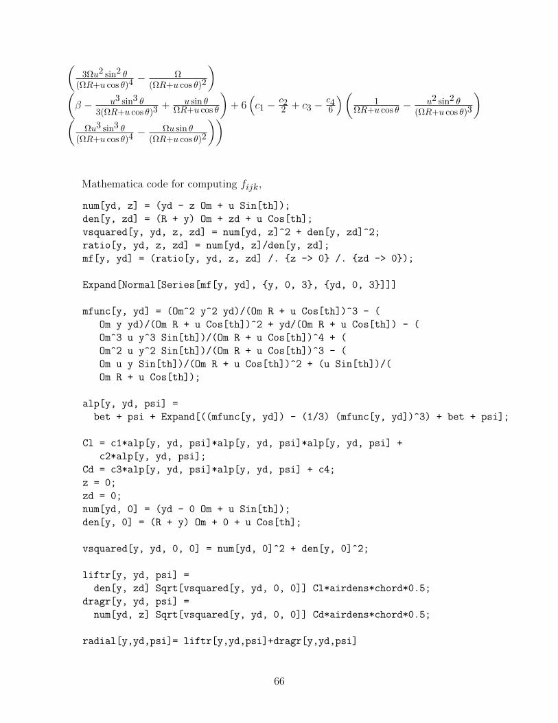
(3Ωu2 sin2 θ


(ΩR+u cos θ)2

)(β − u3 sin3 θ


ΩR+u cos θ

)+ 6

(c1 −

c22 + c3 −

c46

)(1


(ΩR+u cos θ)3

)(



))

Mathematica code for computing fijk,

num[yd, z] = (yd - z Om + u Sin[th]);

den[y, zd] = (R + y) Om + zd + u Cos[th];

vsquared[y, yd, z, zd] = num[yd, z]^2 + den[y, zd]^2;

ratio[y, yd, z, zd] = num[yd, z]/den[y, zd];

mf[y, yd] = (ratio[y, yd, z, zd] /. z -> 0 /. zd -> 0);

Expand[Normal[Series[mf[y, yd], y, 0, 3, yd, 0, 3]]]

mfunc[y, yd] = (Om^2 y^2 yd)/(Om R + u Cos[th])^3 - (

Om y yd)/(Om R + u Cos[th])^2 + yd/(Om R + u Cos[th]) - (

Om^3 u y^3 Sin[th])/(Om R + u Cos[th])^4 + (

Om^2 u y^2 Sin[th])/(Om R + u Cos[th])^3 - (

Om u y Sin[th])/(Om R + u Cos[th])^2 + (u Sin[th])/(

Om R + u Cos[th]);

alp[y, yd, psi] =

bet + psi + Expand[((mfunc[y, yd]) - (1/3) (mfunc[y, yd])^3) + bet + psi];

Cl = c1*alp[y, yd, psi]*alp[y, yd, psi]*alp[y, yd, psi] +

c2*alp[y, yd, psi];

Cd = c3*alp[y, yd, psi]*alp[y, yd, psi] + c4;

z = 0;

zd = 0;

num[yd, 0] = (yd - 0 Om + u Sin[th]);

den[y, 0] = (R + y) Om + 0 + u Cos[th];

vsquared[y, yd, 0, 0] = num[yd, 0]^2 + den[y, 0]^2;

liftr[y, yd, psi] =

den[y, zd] Sqrt[vsquared[y, yd, 0, 0]] Cl*airdens*chord*0.5;

dragr[y, yd, psi] =

num[yd, z] Sqrt[vsquared[y, yd, 0, 0]] Cd*airdens*chord*0.5;

radial[y,yd,psi]= liftr[y,yd,psi]+dragr[y,yd,psi]

66

fhatexpansion[y,yd,psi] =

Normal[Series[radial[y,yd,psi], y, 0, 3, yd, 0, 3, psi, 0, 3]]

From fhatexpansion, the constant and linear coefficients are retained. In the examplebelow TERM0 = f000, TERM1 = f100, TERM2 = f010, TERM3 = f001.

c1 = -2.9916;

c2 = 4.4287;

c3 = 1.185;

c4 = 0.0094;

chord = 0.533;

airdens = 1.292;

lc = 0.1302360914550899;

th = Om*t;

bet = 0;

TERM0 = (airdens*chord*0.5

(Om R + u Cos[th]) Sqrt[(Om R + u Cos[th])^2 +

u^2 Sin[th]^2] (c2 (bet + (u Sin[th])/(Om R + u Cos[th]) - (

u^3 Sin[th]^3)/(3 (Om R + u Cos[th])^3)) +

c1 (bet + (u Sin[th])/(Om R + u Cos[th]) - (u^3 Sin[th]^3)/(

3 (Om R + u Cos[th])^3))^3) +

u Sin[th] Sqrt[(Om R + u Cos[th])^2 +

u^2 Sin[th]^2] (c4 +


3 (Om R + u Cos[th])^3))^2))



u^2 Sin[th]^2] (c2 (-((Om u Sin[th])/(Om R + u Cos[th])^2) + (

Om u^3 Sin[th]^3)/(Om R + u Cos[th])^4) +

3 c1 (-((Om u Sin[th])/(Om R + u Cos[th])^2) + (

Om u^3 Sin[th]^3)/(Om R + u Cos[th])^4) (bet + (u Sin[th])/(

Om R + u Cos[th]) - (u^3 Sin[th]^3)/(

3 (Om R + u Cos[th])^3))^2) + (

Om (Om R +

u Cos[th])^2 (c2 (bet + (u Sin[th])/(Om R + u Cos[th]) - (



3 (Om R + u Cos[th])^3))^3))/

Sqrt[(Om R + u Cos[th])^2 + u^2 Sin[th]^2] +

Om Sqrt[(Om R + u Cos[th])^2 +

u^2 Sin[th]^2] (c2 (bet + (u Sin[th])/(Om R + u Cos[th]) - (



67

3 (Om R + u Cos[th])^3))^3) +

(2 c3 u Sin[th] Sqrt[(Om R + u Cos[th])^2 +

u^2 Sin[th]^2] (-((Om u Sin[th])/(Om R + u Cos[th])^2) + (



3 (Om R + u Cos[th])^3)) + (

Om u (Om R + u Cos[th]) Sin[

th] (c4 +


3 (Om R + u Cos[th])^3))^2))/

Sqrt[(Om R + u Cos[th])^2 + u^2 Sin[th]^2]))



u^2 Sin[th]^2] (c2 (1/(Om R + u Cos[th]) - (

u^2 Sin[th]^2)/(Om R + u Cos[th])^3) +

3 c1 (1/(Om R + u Cos[th]) - (

u^2 Sin[th]^2)/(Om R + u Cos[th])^3) (bet + (u Sin[th])/(


3 (Om R + u Cos[th])^3))^2) + (

u (Om R + u Cos[th]) Sin[

th] (c2 (bet + (u Sin[th])/(Om R + u Cos[th]) - (u^3 Sin[th]^3)/(

3 (Om R + u Cos[th])^3)) +


3 (Om R + u Cos[th])^3))^3))/



u^2 Sin[th]^2] (1/(Om R + u Cos[th]) - (



3 (Om R + u Cos[th])^3)) + (

u^2 Sin[th]^2 (c4 +


3 (Om R + u Cos[th])^3))^2))/


Sqrt[(Om R + u Cos[th])^2 +

u^2 Sin[th]^2] (c4 +


3 (Om R + u Cos[th])^3))^2)))



u^2 Sin[th]^2] (c2 +

3 c1 (bet + (u Sin[th])/(Om R + u Cos[th]) - (u^3 Sin[th]^3)/(

3 (Om R + u Cos[th])^3))^2) +

68


u^2 Sin[th]^2] (bet + (u Sin[th])/(Om R + u Cos[th]) - (

u^3 Sin[th]^3)/(3 (Om R + u Cos[th])^3))))

Mathematica code for computing Mijk,

num[yd, z] = (yd - z Om + u Sin[th]);

den[y, zd] = (R + y) Om + zd + u Cos[th];

vsquared[y, yd, z, zd] = num[yd, z]^2 + den[y, zd]^2;

ratio[y, yd, z, zd] = num[yd, z]/den[y, zd];

mf[y, yd] = (ratio[y, yd, z, zd] /. z -> 0 /. zd -> 0);

Expand[Normal[Series[mf[y, yd], y, 0, 3, yd, 0, 3]]]

mfunc[y, yd] = (Om^2 y^2 yd)/(Om R + u Cos[th])^3 - (

Om y yd)/(Om R + u Cos[th])^2 + yd/(Om R + u Cos[th]) - (

Om^3 u y^3 Sin[th])/(Om R + u Cos[th])^4 + (

Om^2 u y^2 Sin[th])/(Om R + u Cos[th])^3 - (

Om u y Sin[th])/(Om R + u Cos[th])^2 + (u Sin[th])/(

Om R + u Cos[th]);

alp[y, yd, psi] = ((mfunc[y, yd]) - (1/3) (mfunc[y, yd])^3) + bet +

psi;

Momentcof[y, yd, psi] =

alp[y, yd, psi]*(c4 + c2) +

alp[y, yd, psi]*alp[y, yd, psi]*

alp[y, yd, psi]*(c3 + c1 - (c2/2) - (c4/6));

z = 0;

zd = 0;

num[yd, 0] = (yd - 0 Om + u Sin[th]);

den[y, 0] = (R + y) Om + 0 + u Cos[th];

vsquared[y, yd, 0, 0] = num[yd, 0]^2 + den[y, 0]^2;

moment[y, yd, psi] =

Momentcof[y, yd, psi] vsquared[y, yd, 0, 0]*chord*lc*airdens*0.5;

Mhatexpansion[y,yd,psi] =

Normal[Series[moment[y,yd,psi], y, 0, 3, yd, 0, 3, psi, 0, 3]]

From Mhatexpansion, the constant and linear coefficients are retained. In the examplebelow TERM0 = M000, TERM1 = M100, TERM2 = M010, TERM3 = M001.

c1 = -2.9916;

c2 = 4.4287;

c3 = 1.185;

69

c4 = 0.0094;

chord = 0.533;

airdens = 1292;

lc = 0.1302360914550899;

u = 4.72;

th = Om*t;

bet = 0;

R = 6;

TERM0 = 0.5‘ airdens chord lc ((Om R + u Cos[th])^2 +

u^2 Sin[th]^2) ((c2 + c4) (bet + (u Sin[th])/(


3 (Om R + u Cos[th])^3)) + (c1 - c2/2 + c3 - c4/6) (bet + (

u Sin[th])/(Om R + u Cos[th]) - (u^3 Sin[th]^3)/(

3 (Om R + u Cos[th])^3))^3)


u^2 Sin[th]^2) ((c2 +

c4) (-((Om u Sin[th])/(Om R + u Cos[th])^2) + (

Om u^3 Sin[th]^3)/(Om R + u Cos[th])^4) +

3 (c1 - c2/2 + c3 - c4/

6) (-((Om u Sin[th])/(Om R + u Cos[th])^2) + (



3 (Om R + u Cos[th])^3))^2) +

1.‘ airdens chord lc Om (Om R +

u Cos[th]) ((c2 + c4) (bet + (u Sin[th])/(Om R + u Cos[th]) - (

u^3 Sin[th]^3)/(3 (Om R + u Cos[th])^3)) + (c1 - c2/2 + c3 -

c4/6) (bet + (u Sin[th])/(Om R + u Cos[th]) - (

u^3 Sin[th]^3)/(3 (Om R + u Cos[th])^3))^3)


u^2 Sin[th]^2) ((c2 + c4) (1/(Om R + u Cos[th]) - (

u^2 Sin[th]^2)/(Om R + u Cos[th])^3) +

3 (c1 - c2/2 + c3 - c4/6) (1/(Om R + u Cos[th]) - (



3 (Om R + u Cos[th])^3))^2) +

1.‘ airdens chord lc u Sin[

th] ((c2 + c4) (bet + (u Sin[th])/(Om R + u Cos[th]) - (

u^3 Sin[th]^3)/(3 (Om R + u Cos[th])^3)) + (c1 - c2/2 + c3 -

c4/6) (bet + (u Sin[th])/(Om R + u Cos[th]) - (

u^3 Sin[th]^3)/(3 (Om R + u Cos[th])^3))^3)


70

u^2 Sin[th]^2) (c2 + c4 +

3 (c1 - c2/2 + c3 - c4/6) (bet + (u Sin[th])/(


3 (Om R + u Cos[th])^3))^2)

These values of fijk and Mijk are to be used in equation (2.37) ultimately to expressequation (2.44) and finally (2.45) and (2.46).

71

BIBLIOGRAPHY

72

BIBLIOGRAPHY

[1] Annual Energy Outlook 2014 with projections to 2040, U.S. Energy Information Admin-istration, April 2014, DOE-EIA0383(2014)

[2] Picture taken from Johnson System Inc. webpage,http://www.johnsonsysteminc.com/wp-content/uploads/2011/10/Turbine1.jpg

[3] Picture taken from Shanghai StarCreation Group Co., Limited webpage,http://www.shstarcreation.com/0/www.shstarcreation.com/upload/content/201282745650882.jpg.

[4] Eriksson, S., Bernhoff, H., and Leijon, M., 2008. ”Evaluation of different turbine conceptsfor wind power”. Renewable and Sustainable Energy Reviews, 12, pp. 1419-1434.

[5] Barone, M., and Paquette, J., 2012. ”Vertical-axis wind turbines revis-ited: A Sandia perspective”. In 2012 Sandia Wind Turbine Blade Workshop.http://energy.sandia.gov/wp/wp-content/gallery/uploads/3-B-1-Barone-SAND2012-5503C.pdf.

[6] Sutherland, H. J., Berg, D. E., Ashwill, T. D., 2012. ”A Retrospective of VAWT Tech-nology” SAND2012-03014.

[7] Gorban, N. A., Gorlov, A. M., Silantyev, V. M.”Limits of the Turbine Efficiency for FreeFluid Flow”, Journal of Energy Resources Technology, Vol. 123, pages 311 317.

[8] Chiras, D., 2010. Wind Energy Basics: A Green Energy Guide. New Society Publishers,Gabriola Island, BC, Canada.

[9] Dabiri, J. O., 2011. ”Potential order-of-magnitude enhancement of wind farm powerdensity via counter-rotating vertical-axis wind turbine arrays”. Journal of Renewableand Sustainable Energy, 3(4). article number 043104.

[10] Hau, E. ”Wind Turbines Fundamentals, Technologies, Application, Economics”,Springer, Munich, 2012.

[11] Whittlesey, R. W., Liska, S., and Dabiri, J. O., 2010. ”Fish schooling as a basis forvertical axis wind turbine farm design”. Bioinspiration and Biomimetics, 5(3). articlenumber 035005.

73

[12] Kinzel, M., Mulligan, Q., and Dabiri, J. O., 2012. ”Energy exchange in an array ofvertical-axis wind turbines”. Journal of Turbulence, 13(38), pp. 1-13.

[13] Ramakrishnan, V., and Feeny, B. F., 2011. ”In-plane nonlinear dynamics of wind turbineblades”. In ASME International Design Engineering Technical Conferences, 23th BiennialConference on Vibration and Noise. paper number DETC2011-48219, on CD-ROM.

[14] Inoue, T., Ishida, Y., and Kiyohara, T., 2012. ”Nonlinear vibration analysis of the windturbine blade (occurrence of the superharmonic resonance in the out-of-plane vibrationof the elastic blade)”. Journal of Vibration and Acoustics, volume 134, issue 3, 13 pages.

[15] G. Acar, B.F. Feeny, 2014, ”A bend-bend-twist model for horizontal axis wind turbineblades”,, 17thUS National Congress on Theoretical and Applied Mechanics East Lansing.

[16] Kallesøe, B. S., 2007. ”Equations of motion for a rotor blade, including gravity andpitch action”. Wind Energy, 10(3), February, pp. 209230.

[17] B.F. Feeny, 2013, ”Vertical-Axis wind turbine blade vibration modeling” Chemical, Bio-engineering, Environmental and Transports Systems (CBET) proposal no. 1336817 andCivil, Mechanical and Manufacturing Innovation (CMMI) proposal no. 1435126 (2014),National Science Foundation.

[18] Worstell, M. H., ”Aerodynamic Performance of the 17-M-Diameter Darrieus Wind Tur-bine in the Three-Bladed Configuration: An Addendum”, SAND79-1753, August 1982.

[19] Caruntu, D., 2008. ”On nonlinear forced response of nonuniform blades”. In Proceed-ing of the 2008 ASME Dynamic Systems and Control Conference, no. DSCC2008-2157,ASME.

[20] Meirovitch, L., 1997. Principles and Techniques in Vibrations. Prentice Hall, UpperSaddle River.

[21] Jacobs, N. E, Ward, K. E., Pinkerton, R. M., ”The Characteristics of 78 Related AirfoilSections From Tests In The Variable-Density Wind Tunnel”, NACA Report 460.

[22] Worstell, M. H., ”Aerodynamic Performance of the 17 Meter Diameter Darrieus WindTurbine”, SAND78-1737, September 1978.

[23] Charles L. L., Cuyler W. B., Acquilla S. H.,Darrell W. S., 1996, ”Computer ProgramTo Obtain Ordinates for NACA Airfoils”, NASA Technical Memorandum 4741.

74

[24] Dowell, E. H., Curtiss Jr., H. C., Scanlan, R. H., Sisto F., A Modern Course in Aeroe-lasticity, 1989.

[25] Beer, F. P., Johnston, E. R., 1981. Mechanics of Materials. McGraw-Hill.

75

VIBRATIONAL ANALYSIS OF VERTICAL AXIS WIND TURBINE BLADES ... · vibrational analysis of vertical...

Documents

Transcript of VIBRATIONAL ANALYSIS OF VERTICAL AXIS WIND TURBINE BLADES ... · vibrational analysis of vertical...