HAL Id: hal-00894021https://hal.archives-ouvertes.fr/hal-00894021

Submitted on 1 Jan 1994

HAL is a multi-disciplinary open accessarchive for the deposit and dissemination of sci-entific research documents, whether they are pub-lished or not. The documents may come fromteaching and research institutions in France orabroad, or from public or private research centers.

L’archive ouverte pluridisciplinaire HAL, estdestinée au dépôt et à la diffusion de documentsscientifiques de niveau recherche, publiés ou non,émanant des établissements d’enseignement et derecherche français ou étrangers, des laboratoirespublics ou privés.

Bayesian analysis of mixed linear models via Gibbssampling with an application to litter size in Iberian pigs

Cs Wang, Jj Rutledge, D Gianola

To cite this version:Cs Wang, Jj Rutledge, D Gianola. Bayesian analysis of mixed linear models via Gibbs sampling withan application to litter size in Iberian pigs. Genetics Selection Evolution, BioMed Central, 1994, 26(2), pp.91-115. <hal-00894021>

Original article

Bayesian analysis of mixed linear modelsvia Gibbs sampling with an application

to litter size in Iberian pigs

CS Wang JJ Rutledge, D Gianola

University of Wisconsin-Madison, Department of Meat and Animal Science, Madison,WI53706-1284, USA

(Received 26 April 1993; accepted 17 December 1993)

Summary - The Gibbs sampling is a Monte-Carlo procedure for generating random sam-ples from joint distributions through sampling from and updating conditional distribu-tions. Inferences about unknown parameters are made by: 1) computing directly sum-mary statistics from the samples; or 2) estimating the marginal density of an unknown,and then obtaining summary statistics from the density. All conditional distributionsneeded to implement the Gibbs sampling in a univariate Gaussian mixed linear modelare presented in scalar algebra, so no matrix inversion is needed in the computations. Forlocation parameters, all conditional distributions are univariate normal, whereas those forvariance components are scaled inverted chi-squares. The procedure was applied to solvea Gaussian animal model for litter size in the Gamito strain of Iberian pigs. Data were1 213 records from 426 dams. The model had farrowing season (72 levels) and parity (4)as fixed effects; breeding values (597), permanent environmental effects (426) and resid-uals were random. In CASE I, variances were assumed known, with REML (restrictedmaximum likelihood) estimates used as true parameter values. Here, means and variancesof the posterior distributions of all effects were obtained, by inversion, from the mixedmodel equations. These exact solutions were used to check the Monte-Carlo estimatesgiven by Gibbs, using 120 000 samples. Linear regression slopes of true posterior meanson Gibbs means were almost exactly 1 for fixed, additive genetic and permanent environ-mental effects. Regression slopes of true posterior variances on Gibbs variances were 1.00,1.01 and 0.96, respectively. In CASE II, variances were treated as unknown, with a flatprior assigned to these. Posterior densities of selected location parameters, variance com-ponents, heritability and repeatability were estimated. Marginal posterior distributionsof dispersion parameters were skewed, save the residual variance; the means, modes andmedians of these distributions differed from the REML estimates, as expected from theory.The conclusions are: 1) the Gibbs sampler converged to the true posterior distributions,as suggested by CASE I; 2) it provides a richer description of uncertainty about genetic

* Present address: Morrison Hall, Department of Animal Science, Cornell University,Ithaca, NY 14 853-4801, USA

parameters than REML; 3) it can be used successfully to study quantitative genetic varia-tion taking into account uncertainty about all nuisance parameters, at least in moderatelysized data sets. Hence, it should be useful in the analysis of experimental data.

Iberian pig / genetic parameters / linear model / Bayesian methods / Gibbs sampler

Résumé - Analyse bayésienne de modèles linéaires mixtes à l’aide de l’échantillon-nage de Gibbs avec une application à la taille de portée de porcs ibériques.L’échantillonnage de Gibbs est une procédure de Monte-Carlo pour engendrer des échan-tillons aléatoires à partir de distributions conjointes, par échantillonnage dans des dis-tributions conditionnelles réajustées itérativement. Les inférences relatives aux paramètresinconnus sont obtenues en calculant directement des statistiques récapitulatives à partir deséchantillons générés, ou en estimant la densité marginale d’une inconnue, et en calculantdes statistiques récapitulatives à partir de cette densité. Toutes les distributions condi-tionnelles nécessaires pour mettre en ceuvre l’échantillonnage de Gibbs dans un modèleunivarié linéaire mixte gaussien sont présentées en algèbre scalaire, si bien qu’aucune in-version matricielle n’est requise dans les calculs. Pour les paramètres de position, toutesles distributions conditionnelles sont normales univariées, alors que celles des composantesde variance sont des x2 inverses dimensionnés. La procédure a été appliquée à un modèleindividuel gaussien de taille de portée dans la souche porcine ibérique Gamito. Les donnéesreprésentaient 1 21,i observations sur 426 mères. Le modèle incluait les effets fixés de lasaison de mise bas (72 niveaux) et de la parité (4 niveaux) ; les valeurs génétiques in-dividuelles (597), les effets de milieu permanent (426) et les résidus étaient aléatoires.Dans le CAS I, les variances étaient supposées connues, les estimées REML (maximumde vraisemblance restreinte) étant considérées comme les valeurs vraies des paramètres.Les moyennes et les variances des distributions a posteriori de tous les effets étaient alorsobtenues par la résolution du système d’équations du modèle mixte. Ces solutions ex-

actes étaient utilisées pour vérifier les estimées Monte-Carlo données par le Gibbs, enutilisant 120 000 échantillons. Les coefficients de régression linéaire des vraies moyennesa posteriori en fonction des moyennes de Gibbs étaient presque exactement de 1, pourles effets fixés, génétiques additifs et de milieu permanent. Les coeff cients de régressiondes variances vraies a posteriori en fonction des variances de Gibbs étaient 1,00, 1,01, et0, 96 respectivement. Dans le CAS II, les variances étaient traitées comme des inconnues,avec une distribution a priori uniforme. Les densités a posteriori de paramètres de positionchoisis, des composantes de variance, de l’héritabilité et de la répétabilité ont été estimées.Les distributions a posteriori des paramètres de dispersion étaient dissymétriques, sauf lavariance résiduelle; les moyennes, modes et médianes de ces distributions différaient desestimées REML, comme prévu d’après la théorie. On conclut que : i) l’échantillonneurde Gibbs converge vers les vraies distributions a posteriori, comme le suggère le CAS I,ii) il fournit une description de l’incertitude sur les paramètres génétiques plus riche queREML ; iii) il peut être utilisé avec succès pour étudier la variation génétique quantita-tive avec prise en compte de l’incertitude sur tous les paramètres de nuisance, du moinsavec un nombre de données modéré. Il devrait donc être utile dans l’analyse de donnéesexpérimentales.

porc ibérique / paramètres génétiques / modèle linéaire / analyse bayésienne /échantillonnage de Gibbs

INTRODUCTION

Prediction of merit or, equivalently, deriving a criterion for selection is an importanttheme in animal breeding. Cochran (1951), under certain assumptions, showed thatthe selection criterion that maximized the expected merit of the selected animalswas the mean of the conditional distribution of merit given the data. The conditionalmean is known as best predictor, or BP (Henderson, 1973), because it minimizesmean square error of prediction among all predictors. Computing BP requiresknowing the joint distribution of predictands and data, which can seldom be metin practice. To simplify, attention may be restricted to linear predictors.

Henderson (1963, 1973) and Henderson et al (1959) developed the best linearunbiased prediction (BLUP), which removed the requirement of knowing the firstmoments of the distributions. BLUP is the linear function of the data that minimizesmean square error of prediction in the class of linear unbiased predictors.

Bulmer (1980), Gianola and Goffinet (1982), Goffinet (1983) and Fernando andGianola (1986) showed that under multivariate normality, BLUP is the conditionalmean of merit given a set of linearly independent error contrasts. This holds ifthe second moments of the joint distribution of the data and of the predictandare known. However, second moments are rarely known in practice, and must beestimated from the data at hand. If estimated dispersion parameters are used inlieu of the true values, the resulting predictors of merit are no longer BLUP.

In animal breeding, dispersion components are most often estimated using re-stricted maximum likelihood, or REML (Patterson and Thompson, 1971). Theo-retical arguments (eg, Gianola et al, 1989; Im et al, 1989) and simulations (eg,Rothschild et al, 1979) suggest that likelihood-based methods have ability to ac-count for some forms of nonrandom selection, which makes the procedure appealingin animal breeding. Thus, 2-stage predictors are constructed by, first, estimatingvariance and covariance components, and then obtaining BLUE and BLUP of fixedand random effects, respectively, with parameter values replaced by likelihood-based estimates. Under random selection, this 2-stage procedure should convergein probability to BLUE and BLUP as the information in the sample about variancecomponents increases; however, its frequentist properties under nonrandom selec-tion are unknown. One deficiency of this BLUE and BLUP procedure is that errorsof estimation of dispersion components are not taken into account when predictingbreeding values.

Gianola and Fernando (1986), Gianola et al (1986) and Gianola et al (1990a, b,1992) advocate the use of Bayesian methods in animal breeding. The associatedprobability theory dictates that inferences should be based on marginal posteriordistributions of parameters of interest, such that uncertainty about the remainingparameters is fully taken into account. The starting point is the joint posterior den-sity of all unknowns. From the joint distribution, the marginal posterior distributionof a parameter, say the breeding value of an animal, is obtained by successively in-tegrating out all nuisance parameters, these being the fixed effects, all the randomeffects other than the one of interest, and the variance and covariance components.This integration is difficult by analytical or numerical means, so approximationsare usually sought (Gianola and Fernando, 1986; Gianola et al, 1986; Gianola etal, 1990a, b).

The posterior distributions are so complex that an analytical approach is oftenimpossible, so attention has concentrated on numerical procedures (eg, Cantet et al,1992). Recent breakthroughs are related to Monte-Carlo Markov chain proceduresfor multidimensional integrations and for sampling from joint distributions (Gemanand Geman, 1984; Gelfand and Smith, 1990; Gelfand et al, 1990). One of theseprocedures, Gibbs sampling, has been studied extensively in statistics (Gelfandand Smith, 1990; Gelfand et al, 1990; Besag and Cliford, 1991; Gelfand and Carlin,1991; Geyer and Thompson, 1992).Wang et al (1993) described the Gibbs sampler for a univariate mixed lin-

ear model in an animal breeding context. They used simulated data to constructmarginal densities of variance components, variance ratios and intraclass correla-tions, and noted that the marginal distributions of fixed and random effects couldalso be obtained.

However, their implementation was in matrix form. Clearly, some matrix com-putations are not feasible in many animal breeding data sets because inversion oflarge matrices is needed repeatedly.

In this paper, we consider Bayesian marginal inferences about fixed and randomeffects, variance components and functions of variance components in a univariateGaussian mixed linear model. Here, marginal inferences are obtained, in contrastto Wang et al (1993) through a scalar version of the Gibbs sampler, so inversion ofmatrices is not needed. Our implementation was applied to and validated with adata set on litter size of Iberian pigs.

THE GIBBS SAMPLER FOR THE GAUSSIAN MIXED LINEARMODEL

Model

We consider a univariate mixed linear model with several independent randomfactors as in Henderson (1984), Macedo and Gianola (1987) and Gianola et al

(1990a, b):

where: y: data vector of order n x 1; X: known incidence matrix of order n x p ;Zi: known matrix of order n x qi ; (3: p x 1 vector of uniquely defined ’fixed effects’(so that X has full column rank); ui: qi x 1 random vector; and e: n x 1 vector ofrandom residuals.

The conditional distribution that generates the data is:

where I is an n x n identity matrix, and Qe is the variance of the random residuals.

Prior Distributions

An integral part of Bayesian analysis is the assignment of prior distributions to allunknowns in the model; here, these are 13, Ui (i = 1, 2, ... , c) and the c + 1 variancecomponents (one for each of the random vectors, plus the error). Usually, a flat oruniform prior distribution is assigned to 0, so as to represent lack of prior knowledgeabout this vector, so:

Further, it is assumed that:

where Gi is a known matrix and cr! is the variance of the prior distribution ofui. In a genetic context, Gi matrices can contain functions of known coefficientsof coancestry. All ui’s are assumed to be mutually independent a priori, as well asindependent of j3. Note that the priors for ui correspond to the assumptions madeabout these random vectors in the classical linear model.

Independent scaled inverted chi-square distributions are used as priors forvariance components, so that:

and

Above, ve(v&dquo;!) is a ’degree of belief’ parameter, and s!(s!) can be thought of as aprior value of the appropriate variance.

Joint posterior density

be 0’ without 0z. Further, let

be the vector of variance components other than the residual;

and

be the sets of all prior variances and degrees of belief, respectively. As shown, forexample, by Macedo and Gianola (1987) and Gianola et al (1990a, b), the jointposterior density is in the normal-gamma form:

Inferences about each of the unknowns (9, v, !e ) are based on their respectivemarginal densities. Conceptually, each of the marginal densities is obtained bysuccessive integration of the joint density [7] with respect to parameters other thanthe one of interest. For example, the marginal density of a£ is

It is difficult to carry out the needed integration analytically. Gibbs sampling is aMonte-Carlo procedure to overcome such difficulties.

liblly conditional posterior densities (Gibbs sampler)

The fully conditional posterior densities of all unknowns are needed for implement-ing the Gibbs sampling. Each of the full conditional densities can be obtained byregarding all other parameters in [7] as known. Let W = f wij 1, i, j = 1, 2, ... , N,and b = {bi}, i = 1, 2, ... , N be the coefficient matrix and the right hand side ofthe mixed model equations, respectively. As proved in the APpendix, the conditionalposterior distribution of each of the location parameters in 0 is normal, with meanand variance !i and Ez :

because all computations needed to implement Gibbs sampling are scalar, withoutany required inversion of matrices. This is in contrast with the matrix version ofthe conditional posterior distributions for the location parameters given by Wanget al (1993). It should be noted that distributions [8] do not depend on s and v,because v is known in [8]. ..

The conditional posterior density of o,2 is in the scaled inverted chi-square form:

It can be readily seen that

with parameters

Each condition posterior density of a u! 2 is also in the scaled inverted chi-squareform:

A set of the N + c + 1 conditional posterior distributions [8]-[10] is called theGibbs sampler for our problem.

FULL CONDITIONAL POSTERIOR DENSITIES UNDER SPECIALPRIORS

The Gibbs sampler with ’naive’ priors for all variance components

The Gibbs sampler [8]-[10] given above is based on scaled inverted chi-squaresused as priors for the variance components. These priors are proper and, therefore,informative, about the variance. A possible way of representing prior ignoranceabout variances would be to set the degree of belief parameters of the priordistributions for all the variance components to zero ie, ve = vu, = 0, for all i.These priors have been used, inter alia, by Gelfand et al (1990) and Gianola etal (1990a, b). In this case, the conditional posterior distributions of the locationparameters are as in !8!:

because the distributions do not depend on s and v.However, the conditional posterior distributions of the variance components no

longer depend on hyper-parameters s and v. The conditional posterior distributionof the residual variance remains in the scaled inverted chi-square form:

but now with parameters

Each conditional posterior density of a), is again in the scaled inverted

chi-square form:

with parameters v&dquo;! = qi and Vui = u§Gy lui/v&dquo;!.It has been noted recently (Besag et al, 1991; Raftery and Banfield, 1991) that

under these priors, the joint posterior density [7] is improper because it does notintegrate to 1. In the light of this, we do not recommend these ’naive’ priors forvariance component models.

The Gibbs sampler with flat priors for all variance components

Under flat priors for all variance components, ie p(v, (J’!) oc constant, the Gibbssampler is as in !11!-!13!, except that ve = n - 2 and Vu, = qi - 2 for i = 1,2,..., c.This version of the sampler can also be obtained by setting V, = -2 in [9] andv = (-2, -2, ... , -2)’ and s = (0, 0, ... , 0)’ in [10]. With flat priors, the jointposterior density [7] is proper.

The Gibbs sampler when all variance components are known

When variances are assumed known, the only conditional distributions needed arethose for the location parameters, and these are as in [8] or !11!.

INFERENCES ABOUT THE MARGINAL DISTRIBUTIONSTHROUGH GIBBS SAMPLING

Gibbs sampling: an overview

The Gibbs sampler was used first in spatial statistics and presented formally byGeman and Geman (1984) in an image restoration context. Applications to Bayesianinference were described by Gelfand and Smith (1990) and Gelfand et al (1990).Since then, it has received extensive attention, as evidenced by recent discussionpapers (Gelman and Rubin, 1992; Geyer, 1992; Besag and Green, 1993; Gilks etal, 1993; Smith and Roberts, 1993). Its power and usefulness as a general statisticaltool to generate samples from complex distributions arising in some particularproblems is unquestioned.

Our purpose is to generate random samples from the joint posterior distribu-tion !7!, through successively drawing samples from and updating the Gibbs sam-pler !8!-!10!. Formally, Gibbs sampling works as follows:

(i) set arbitrary initial values for e, v and a e 2(ii) generate Oi from [8] and update Bi, i = 1, 2, ... , N ;

(iii) generate u2 from [9] and update Qe ;(iv) generate u2i from [10] and update a-!i’ i = 1,2,..., c;(v) repeat (ii)-(iv) k (length of the chain) times.

As k - oo, this creates a Markov chain with an equilibrium distribution that has[7] as its density. We shall call this procedure a single long-chain algorithm.

In practice, there are at least 2 ways of running the Gibbs sampler: a single longchain and multiple short chains. The multiple short-chain algorithm repeats steps(i)-(v) m times and saves only the kth iteration as sample (Gelfand and Smith,1990; Gelfand et al, 1990). Based on theoretical arguments (Geyer, 1992) and onour experience, we used the single long-chain method in the present study.

Initial iterations are usually not stored as samples on grounds that the chain maynot yet have reached the equilibrium distribution; this is called ’warm-up’. Afterthe warm-up, samples are stored every d iterations, where d is a small positiveinteger. Let the total number of samples saved be m, the sample size.

If the Gibbs sampler converges to the equilibrium distribution, the m samplesare random drawings from the joint posterior distribution with density !7!. The ithsample

joi,vi and (!)J,z=l,2,...,! [14]is then an N + c + 1 vector, and each of the elements of this vector is a drawingfrom the appropriate marginal distribution. Note that the m samples in [14] areidentically but not independently distributed (eg, Geyer, 1992). We call m samplesin [14] as Gibbs samples for reference.

Density estimation and Bayesian inference based on the Gibbs samples

Suppose xi, i = 1, 2, ... , m is one of the components [14], ie a realization from

running the Gibbs sampler of variable x. The m (dependent) samples can be usedto compute features of the posterior distribution P(x) by Monte-Carlo integration.An intevral

!

u = J g(x)dP(x) [15]

can be approximated by

where g(x) can be any feature of P(x), such as its mean or variance. As m - 00, uconverges almost surely to u (Geyer, 1992).

Another way to compute features of P(x) is by first estimating the densityp(x), and then obtaining summary statistics from the estimated density using 1-dimensional numerical procedures. If Yi(i = 1, 2, ... , m) is another component of(14!, an estimator of p(x) is given by the average of the m conditional densitiesp(xlyi) (Gelfand and Smith, 1990):

Note that this estimator does not use the samples xi, i = 1, 2, ... , m; instead,it uses the samples of variable y through the conditional density p(x!y). Thisprocedure, though developed primarily for identically and independently distributed(iid) data, can also be used for dependent samples, as noted by Liu et al (1991) andDiebolt and Robert (1993).An alternative form of estimating p(x) is to use samples xi(i = 1,2,..., m) only.

For example, a kernel density estimator is defined (Silverman, 1986) as:

where j!(z) is the estimated density at point z, K(.) is a ’kernel function’, and h isa fixed constant called window width; the latter determines the smoothness of theestimated curve. For example, if a normal density is chosen as kernel function, then[18] becomes:

Again, though the kernel density estimator was developed for iid data, the work ofYu (1991) indicates that the method is valid for dependent data as well.

Once the density of p(x) is estimated by either [17] or !19!, summary statistics(eg, mean and variance) can be computed by a 1-dimensional numerical integrationprocedure, such as Simpson’s rules. Probability statements about x can also bemade, thus providing a full Bayesian solution to inferences about the distribution x.

Bayesian inference about functions of the original parameters

Suppose we want to make inference about the function:

The quantity

is a random (dependent) sample of size m from a distribution with density p(z).Formulae !16!, [18] and [19] using such samples can also be used to make inferencesabout z.An alternative is to use standard techniques to transform from either the

conditional densities p(x!y) or p(y!x), to p(z!y) or p(z!x). Let the transformationbe from xly to z!y; the Jacobian of the transformation is lyl, so the conditionaldensity of zly is:

An estimator of p(z), obtained by averaging m conditional densities of p(zly), is

APPLICATION OF GIBBS SAMPLING TO LITTER SIZE IN PIGS

Data

Records were from the Gamito strain of Iberian pigs, Spain. The trait consideredwas number of pigs born alive per litter. Details about this strain and the data arein Dobao et al (1983) and Toro et al (1988); Perez-Enciso and Gianola (1992) gaveREML estimates of genetic parameters. Briefly, the data were 1213 records from426 dams (including 68 crossfostered females). There were 72 farrowing seasons and4 parity classes as defined by Perez-Enciso and Gianola (1992).

Model

A mixed linear model similar to that of Perez-Enciso and Gianola (1992) was:

where y is a vector of observations (number of pigs born alive per litter); X, Ziand Z2 are known incidence matrices relating (3, u and c, respectively, to y; 13 isa vector of fixed effects, including a mean, farrowing season (72 levels) and parity(4 levels) ; u is a random vector of additive genetic effects (597 levels) ; c is a randomvector of permanent environmental effects (426 levels) ; and e is a random vectorof residuals. Distributional assumptions were:

where Qu, a! and cr! are variance components and A is the numerator of Wright’srelationship matrix; the vectors u, c and e were assumed to be pairwise indepen-dent. After reparameterization, the rank (p) of X was 1 + 71 + 3 = 75; the rank ofthe mixed model equations was then: N = 75 + 597 + 426 = 1 098.

Gibbs sampling

We ran 2 separate Gibbs samplers with this data set, and we refer to these analysesas CASES I and II. In CASE I, the 3 variance components were assumed known,with REML estimates (Meyer, 1988) used as true parameter values. In CASE II,the variance components were unknown, and flat priors were assigned to them. Foreach of the 2 cases, a single chain of size 1 205 000 was run. After discarding thefirst 5 000 iterations, samples were saved every 10 iterations (d = 10), so the totalnumber of samples (m) saved was 120 000. This specification (mainly the length ofa chain) of running the Gibbs sampler was based on our own experience with thisdata and with others. It may be different for other problems.

Due to computer storage limitation, not all Gibbs samples and conditionalmeans and variances could be saved for all location parameters. Instead, forfurther analysis and illustration, we selected 4 location parameters arbitrarily,one from each of the 4 factors (farrowing season, parity, additive genetic effectand permanent environmental effect). For each of these 4 location parameters, thefollowing quantities were stored:

where xi is a Gibbs sample from an appropriate marginal distribution, and 01 and

vi are the mean and variance of the conditional distribution, [8] or !11J, used forgenerating xi at each of the Gibbs steps.

In CASE II, we also saved the m Gibbs samples for each of the variance

components, and

where si is the scale parameter appearing in the conditional density [9] or [10] ateach of the Gibbs iterations.A FORTRAN program was written to generate the samples, with IMSL subrou-

tines used for drawing random numbers (IMSL, INC, 1989).

Density estimation and inferences

For each of the 4 selected location parameters (CASES I and II) and the 3 variancecomponents, we estimated the marginal posterior with estimators [17] and !19!, ieby averaging m conditional densities and by the normal kernel density estimationmethod, respectively. Estimator [17] of the density of a location parameter wasexplicitly:

where 0j and 11j are the conditional mean and variance of the conditional posteriordensity of z. For each of the variance components, the estimator was:

where v is the degree of belief, sj is the scale parameter of the conditional posteriordistribution of the variance of interest, and r(.) is the gamma function. The normalkernel estimator [19] was applied directly to the samples for location and dispersionparameters.

To estimate the densities, we divided the ’effective domain’ of each parameterinto 100 equally spaced intervals; the effective domain contained at least 99.5%of the density mass. Running through the effective domain, a sequence of pairs(p(zi), zi), i = 1, 2, ... ,101, was generated. Densities were displayed graphically byplotting (p(zi), zi) pairs. For the normal kernel density estimator (19!, window widthwas specified as: h = (range of effective domain)/75.

For the 4 selected location parameters, the mean, mode, median and variance ofeach of the marginal distributions were computed as summary features. The mean,

median and variance were obtained with Simpson’s integration rules by furtherdividing the effective domain into 1 000 equally spaced intervals, and using a cubicspline technique (IMSL, INC, 1989); the mode was located through a grid search.For location parameters other than the 4 selected ones, the posterior means andvariances were computed directly from the Gibbs samples.

Density estimation for functions of variance components

As mentioned previously, the posterior density of any function of the originalparameters can be made through transformation of random variables withoutrerunning the Gibbs sampler, provided appropriate samples are saved. In this

section, we summarize methods for density estimation of functions of variancecomponents; see also Wang et al (1993).

Let the Gibbs samples for or2,a2 and or2 , be respectively:

Also, let the scale parameters of the corresponding densities be:

and

Consider first estimating the marginal posterior density of the total variance:

QP = a2 + a§ c 2+U2 . e Let the transformation be from the conditional posterior density,(0,2 e 1 y, e, s, v) to ( 01; 2 1 y, 0, v, s, v). The Jacobian of the transformation is 1. Thus,using !17!, the estimator of the marginal posterior density of or; is:

where v = ve. Further, zpi = Xui + x!i + xei, (i = 1, 2, ... , m), is a sample from themarginal distribution’ of o-!.

Similarly, the estimator of the marginal posterior density of h2 = C2/ u 01; isobtained by using the transformation afl - h2 in the conditional posterior densityof a2. One obtains

where v = iu and

For repeatability, r = (Qu + 0,2)/U,2, we used the transformation o! &mdash;! r in theconditional posterior density of Qe to obtain

where c is as in [33] but with v = ve.If one wishes to make inferences about the variance ratio, !y = (]&dquo;!/(]&dquo;!, the

trasnformation u2 -> q yields the estimator of the marginal posterior density of !.

where v = vu. The variance ratio, 6 = or2/or2, is estimated in the same mammer asfor q in [35] with the samples Scj substituted in place of s!! and v = using thetransformation o,2 c 6.

RESULTS

When variance components are known (CASE I), the marginal posterior distribu-tions of all location parameters are normal (Gianola and Fernando, 1986). The mean(mode or median) of the marginal distribution of a location parameter is given bythe corresponding component of the solution vector of the mixed model equations,and the variance of the distribution is equal to the corresponding diagonal elementof the inverted mixed model coefficient matrix, multiplied by the residual variance.These are mathematical facts, and do not relate in any way to the Gibbs sampler.We used this knowledge to assess the convergence of the Gibbs sampler, which givesMonte-Carlo estimates of the posterior means and variances. In CASE I, for thedata at hand, the posterior distributions can be arrived at more efficiently by directinversion or iterative methods than via the Gibbs sampler.

Table I contains results of a comparison between the posterior means andvariances estimated by Gibbs sampling (GIBBS) with the exact values found bysolving directly the mixed model equations (TRUE). Several criteria were usedto compare the 2 sets of results: absolute difference (bias) between TRUE andGIBBS; absolute relative bias (RB) defined as bias divided by TRUE; the slopesof the linear regression of TRUE on GIBBS, and vice versa; and the correlationbetween TRUE and GIBBS. Of course, GIBBS and TRUE were not exactly thesame because GIBBS is subject to Monte-Carlo sampling errors; as m(k) goes toinfinity, GIBBS is expected to converge to TRUE. We found excellent agreement

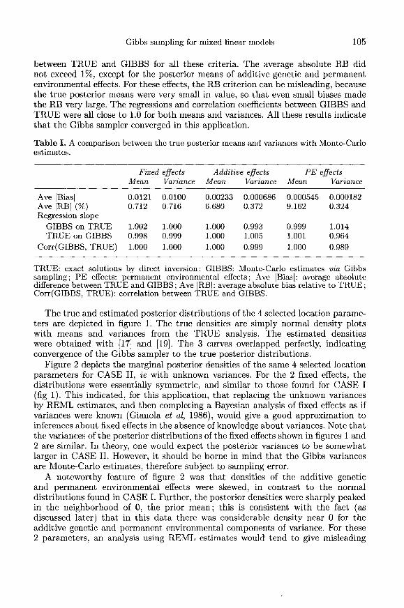
between TRUE and GIBBS for all these criteria. The average absolute RB didnot exceed 1%, except for the posterior means of additive genetic and permanentenvironmental effects. For these effects, the RB criterion can be misleading, becausethe true posterior means were very small in value, so that even small biases madethe RB very large. The regressions and correlation coefficients between GIBBS andTRUE were all close to 1.0 for both means and variances. All these results indicatethat the Gibbs sampler converged in this application.

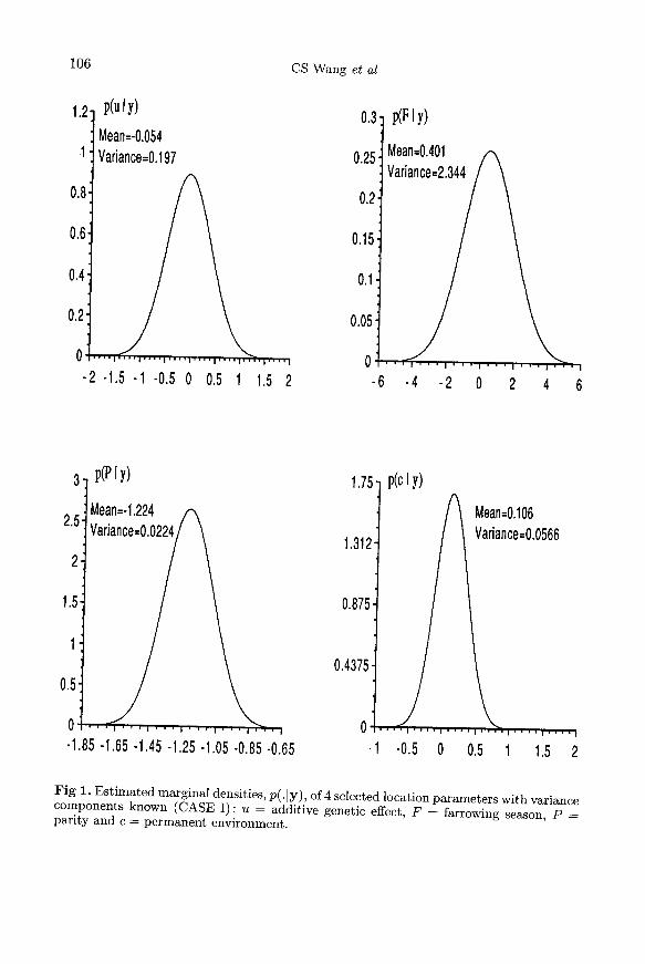
The true and estimated posterior distributions of the 4 selected location parame-ters are depicted in figure 1. The true densities are simply normal density plotswith means and variances from the TRUE analysis. The estimated densitieswere obtained with [17] and [19]. The 3 curves overlapped perfectly, indicatingconvergence of the Gibbs sampler to the true posterior distributions.

Figure 2 depicts the marginal posterior densities of the same 4 selected locationparameters for CASE II, ie with unknown variances. For the 2 fixed effects, thedistributions were essentially symmetric, and similar to those found for CASE I(fig 1). This indicated, for this application, that replacing the unknown variancesby REML estimates, and then completing a Bayesian analysis of fixed effects as ifvariances were known (Gianola et al, 1986), would give a good approximation toinferences about fixed effects in the absence of knowledge about variances. Note thatthe variances of the posterior distributions of the fixed effects shown in figures 1 and2 are similar. In theory, one would expect the posterior variances to be somewhatlarger in CASE II. However, it should be borne in mind that the Gibbs variancesare Monte-Carlo estimates, therefore subject to sampling error.A noteworthy feature of figure 2 was that densities of the additive genetic

and permanent environmental effects were skewed, in contrast to the normaldistributions found in CASE I. Further, the posterior densities were sharply peakedin the neighborhood of 0, the prior mean; this is consistent with the fact (asdiscussed later) that in this data there was considerable density near 0 for theadditive genetic and permanent environmental components of variance. For these2 parameters, an analysis using REML estimates would tend to give misleading

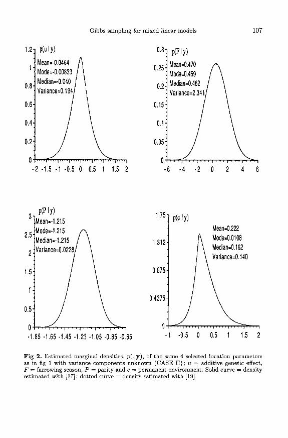
probability statements and posterior confidence intervals. In particular, in CASE I,the posterior mean (variance) of the selected permanent environmental effect was0.106 (0.0566); in CASE II, the corresponding figure was 0.22 (0.140). The datacontained little information about the permanent environmental effect of this

animal, and this is proportional to the number of litters produced by the sowin question. It is precisely in these instances that ’errors’ in variance componentestimates are crucial. The posterior variance of the permanent environmental effectin CASE II was almost twice as large as in CASE I, illustrating the impact oferrors in estimating variance components on inferences. The point is that variances,interval estimates and probability statements about location parameters based onnormal approximations, with variance components assumed known in the mixedmodel equations, can be misleading when information about location parametersand variances is scant in the data. The more information one has about a location

parameter, the less influential are the assumed values for the variance components.The problem could be serious if the number of location parameters is large relativeto the number of observations, eg, in an animal model, and if the data do not containsufficient information about the variance parameters. An exact Bayesian analysissuch as the one conducted here for CASE II would correct all these problems.

Estimated densities for variance components and their functions are presentedin figure 3. REML estimates (Meyer, 1988) are also included for comparisonpurposes. The striking feature was that all distributions, with the exception ofthose of the residual and phenotypic variances, were skewed. Hence, the mean,mode and median tended to differ from each other. Consider, for example, theposterior distribution of the additive genetic variance; the REML estimate was0.206, identical to the estimated posterior mean, but quite different from themarginal mode (0.165). For o, c 2, the REML estimate was closer to the marginal modethan to the mean or median. A naive 95% ’confidence interval’ for U2 based on themean and variance of the posterior distribution and asymptotic theory would be(-0.052, 0.309) ; inference of this type is typical in likelihood based analyses. In thelight of the Bayesian analysis depicted in figure 3, the hypothesis that the permanentenvironmental variance is zero could not be rejected, although there is considerableposterior probability that Q! > 0.04. Further, whereas any reasonable Bayesianconfidence interval would be in the permissible parameter space, an REML intervalwould not in this case. For this data set, 95% asymptotic confidence intervals fora2 and a§ based on the REML analysis were (-0.971, 1.356) and (-0.267, 0.384),respectively.

The estimated densities using [17] were less smooth than those based on !19).This was due to Monte-Carlo sampling errors; the curves can be smoothed byincreasing the length of the chain.

DISCUSSION

A Gibbs sampling scheme was developed for a univariate Gaussian mixed linearmodel with correlated observations, such as those arising in quantitative genetics.With this implementation, a full Bayesian analysis of the location and dispersionparameters, or of their functions, in a real-life mixed linear model was possible.The Gibbs sampler made feasible integration of all nuisance parameters, and gave

a Monte-Carlo estimate of the marginal posterior distribution of the parameter ofinterest. In the classical sense, this is equivalent to taking into account errors inestimation of all other parameters in the model when inferences about a parameterof interest are made. This is precisely why REML was advanced over maximumlikelihood: errors in estimating fixed effects are taken into account in REML. Inthis sense, a marginal Bayesian analysis with flat priors can be thought of as ananalysis of a marginal likelihood, with additional richness brought by the probabilitycalculus on which Bayesian inference is based.

Bayesian analysis via Gibbs sampling provides the complete marginal posteriordistribution of an unknown. Any features of this distribution can be computed,including probability statements. Because Bayes theorem operates within the spacein which parameters are defined, all statistics fall in the permissible parameterspace. This is a serious problem of frequentist procedures such as REML. Althoughthe REML estimates are defined within the permissible parameter space, intervalestimates based on asymptotic theory can include values outside its boundaries, asillustrated previously.

Unfortunately, a richer analysis requires more intensive computations. For theproblem studied in this paper, it took about 14.5 and 23 hours of CPU for CASES Iand II, respectively, on a HP9000/827 running HPUX 8.02, with a Gibbs chainlength of 1205 000. This certainly limits the applicability of the procedure to largeproblems, at least at present. Our experience suggests that the procedure is feasiblewith as many as 10 000 location parameters; hence, analysis of data from designedexperiments would be feasible. With the fast advances in computing technology, itis likely that much larger models could be handled efficiently in the near future. Wedo not advocate at this time Gibbs sampling as a computing method for routinegenetic evaluation. However, it is appealing for scientific purposes, eg, when manysimplifying assumptions must be relaxed, or when model flexibility is needed.

The chain length of 1 205 000 was deliberately long. Summary statistics of amarginal distribution can be computed from a much shorter chain in practice, withrelatively high precision. This, of course, would reduce computing cost.

Theoretical results guarantee that an irreducible Markov chain converges to itsequilibrium distribution (Kipnis and Varadhan, 1986; Tierney, 1991). However,this does not translate easily into practical guidelines for convergence checking.Our heuristic convergence checking procedure was to run chains under differentspecifications (starting values, chain length and number of samples saved) of thesampler. If they produced similar results, convergence was assumed. Our experiencesuggested that if one can obtain a smooth density curve by averaging conditionals,as in [17], the sampler has converged. In CASE II, a smooth curve using [17]was much harder to obtain for dispersion than for location parameters; with !17!,very long chains were needed to obtain smooth estimated densities. In CASE I,convergence was sure, because the estimated densities were almost identical tothose derived by analytical means. At any rate, checking for convergence is adifficult problem in most areas of numerical analysis, and Gibbs sampling is no

exception. Here, there are additional complications stemming from Monte-Carloerrors and from convergence in probability to the true distributions. In the processof monitoring convergence, we observed that this was slower for or and a§ than forother parameters.

We used 2 density estimators: averaging conditionals [17] and the normal

density estimation [19]. Theoretically, [17] is expected to be more efficient thanits counterpart because of the use of conditional information (Gelfand and Smith,1990). However, we did not observe sizable differences in our analysis, as can beascertained from figures 1-3. In fact, we found that similar density estimates couldbe obtained with [19], but using much fewer samples than 120000. This wouldfavor [19] over (17!, in this situation. The naive fixed window length used in [19]throughout performed well in all cases.

The procedure can be divided into 2 stages: Gibbs sampling and post-Gibbsanalysis. In our case, because sample size was large (m = 120 000), the postGibbs analysis was onerous. In general, large sample sizes are needed becauseof high serial correlations between consecutive samples. The effective sample size,perhaps measured as m(1 - p)!(1 + p) (Tierney, 1991), where p is the lag-oneserial correlation, could be much smaller than m. For example, if p = 0.9, theeffective sample size would be 6 316, or 5.26% of 120 000. In our study, we monitoredserial correlations between consecutive drawings for the variance components. Theestimated lag-300 correlations for Qu and a§ were 0.6 and 0.3, respectively, whilethe lag-one correlation for a£ was almost 0. This is why the chains were so long,and so many samples were saved.

One possible way to reduce dependence between samples would be to embed aHasting or Metropolis updating step in the basic Gibbs sampling scheme, as used,for example, in pedigree analysis (Lin and Thompson, 1993). Further research isneeded in this area for the type of models applied in animal breeding.We have demonstrated in this paper that the Gibbs sampling scheme can be

used successfully to carry out an exact Bayesian analysis of all parameters ina general univariate mixed linear model. The method, however, could also beused in classical situations for problems where analytical integration is intractable.Examples are Besag and Cliford (1989, 1991) on Monte-Carlo tests, and Geyerand Thompson (1992) or Gelfand and Carlin (1991) on Monte-Carlo maximumlikelihood. Extensions to multivariate problems, eg, genetic maternal effects, are inprogress (Jensen et al, 1994). An application of Gibbs sampling to the analysis ofselection experiment is given by Wang et al (1994).

ACKNOWLEDGMENTS

We thank the College of Agricultural and Life Sciences (CALS), University of Wisconsin-Madison, and the National Pork Producer Council, USA, for supporting this work.Computations were made on the HP9000/827 of CALS, with additional computingresources generously provided by the San Diego Supercomputer Center. M Perez-Encisois thanked for kindly providing the data, and M Newton is thanked for useful suggestions.We thank 2 anonymous reviewers for comments on the paper.

REFERENCES

Besag J, Cliford P (1989) Generalized Monte-Carlo significance tests. Biometrika76, 633-642Besag J, Cliford P (1991) Sequential Monte-Carlo p-values. Biometrika 78, 301-304

Besag J, Green PJ (1993) Spatial statistics and Bayesian computation (withdiscussion). J R Statist Soc B 55, 25-37Besag J, York J, Mollie A (1991) Bayesian image restoration with two applicationsin spatial statistics (with discussion). Ann Inst Statist Math 43, 1-59Bulmer MG (1980) The Mathematical Theory of Quantitative Genetics. ClarendonPress, OxfordCantet RJC, Fernando RL, Gianola D (1992) Bayesian inference about dispersionparameters of univariate mixed models with maternal effects: theoretical consider-ations. Genet Sel Evol 24, 107-135Cochran WG (1951) Improvement by means of selection. Proc 2nd BerkeleySymposium (J Neyman ed) Math Stat and Prob, University of California Press,Los Angles, CA, 449-470Diebolt J, Robert CP (1993) J R Statist Soc B 55, 71-72Dobao MT, Rodriganez J, Silio L (1983) Seasonal influence on fecundity and litterperformance characteristics in Iberian pigs. Livest Prod Sci 10, 601-610Fernando RL, Gianola D (1986) Effect of assortative mating on genetic change dueto selection. Theor Appl Genet 72, 395-404Gelfand AE, Carlin BP (1991) Maximum likelihood estimation for constrained ormissing data models. Research report 91-002, Division of Biostatistics, Universityof MinnesotaGelfand AE, Hills SE, Racine-Poon A, Smith AFM (1990) Illustration of Bayesianinference in normal data models using Gibbs sampling. J Am Stat Assoc 85, 972-985Gelfand AE, Smith AFM (1990) Sampling-based approaches to calculating marginaldensities. J Am Stat Assoc 85, 398-409Gelman A, Rubin DB (1992) Inference from iterative simulation using multiplesequences (with discussion). Stat Sci 7, 467-511 lGeman S, Geman D (1984) Stochastic relaxation, Gibbs distributions and theBayesian restoration of images. IEEE Transactions on pattern analysis and machineintelligence 6, 721-741Geyer CJ (1992) Practical Markov chain Monte Carlo. Stat Sci 7, 467-511Geyer CJ, Thompson EA (1992) Constrained Monte Carlo maximum likelihood fordependent data. J R Stat Soc B 54, 657-699Gianola D, Goffinet B (1982) Sire evaluation with best linear unbiased predictors.Biometrics 38, 1085-1088Gianola D, Fernando RF (1986) Bayesian methods in animal breeding theory.J Anim Sci 63, 217-244Gianola D, Foulley JL, Fernando RL (1986) Prediction of breeding values whenvariances are not known. Genet ,5’el Evol 18, 485-498Gianola D, Fernando RL, Im S, Foulley JL (1989) Likelihood estimation of quan-titative genetic parameters when selection occurs: models and problems. Genome31, 768-777Gianola D, Im S, Macedo FWM (1990a) A framework for prediction of breedingvalue. In: Advances in Statistical Methods for Genetic Improvement of Livestock(D Gianola, K Hammond, eds) Springer-Verlag, New York, 210-239Gianola D, Im S, Fernando RL, Foulley JL (1990b) Mixed model methodologyand the Box-Cox theory of transformations: a Bayesian approach. In: Advances in

Statistical Methods for Genetic Improvement of Livestock (D Gianola, K Hammond,eds), Springer-Verlag, New York, 15-40Gianola D, Foulley JL, Fernando RL, Henderson CR, Weigel KA (1992) Estimationof Heterogeneous variances using empirical Bayes methods: theoretical considera-tions. J Dairy Sci 75, 2805-2823Gilks WR, Clayton DG, Spiegelhalter DJ, Best NG (1993) Modeling complexity:applications of Gibbs sampling in medicine (with discussion). J R Statist Soc B 55,39-52Goffinet B (1983) Selection on selected records. Genet Sel Evol 15, 91-98Henderson CR (1963) Selection index and expected genetic advance. In: StatisticalGenetics and Plant Breeding (WD Hanson, HF Robinson, eds) NAS-NRC 982,Washington, DCHenderson CR (1973) Sire evaluation and genetic trends. In: Proceedings of theAnimal Breeding and Genetics Symposium in Honor of Dr Jay L Lush. ASAS andADSA, Champaign, 11Henderson CR (1984) Applications of linear models in animal breeding. Universityof Guelph, Guelph, CanadaHenderson CR, Kempthorne 0, Searle SR, von Krosigk CM (1959) The estimationof environmental and genetic trends from records subject to culling. Biometrics 15,192-218Im S, Fernando RL, Gianola D (1989) Likelihood inferences in animal breedingunder selection: a missing data theory view point Genet Sel Evol 21, 399-414IMSL, INC (1989) IMSL2, STAT/LIBRARY: FORTRAN Subroutines for StatisticalAnalysis. Houston, TexasJensen J, Wang CS, Sorensen DA, Gianola D (1994) Bayesian inference on varianceand covariance components for traits influenced by maternal and direct geneticeffects using Gibbs sampler. Acta Agric Scandinavica (in press)Kipnis C, Varadhan SRS (1986) Central limit theorem for additive functionals ofreversible Markov processes and applications to simple exclusions. Commun MathPhys 104, 1-19Lin S, Thompson EA (1993) J R Statist Soc B 55, 81-82Liu J, Wong W, Kong A (1991) Correlation structure and convergence rate of theGibbs sampler. Technical report 304. Dept of statistics, University of ChicagoMacedo FWM, Gianola D (1987) Bayesian analysis of univariate mixed models withinformative priors. Eur Assoc Anim Prod, 38th Annu Meet, Lisbon, Portugal, 35Meyer K (1988) DFREML - A set of programs to estimate variance componentsunder an individual animal model. J Dairy Sci 71 (Supple 2), 33-34Patterson HD, Thompson R (1971) Recovery of interblock information when blocksizes are unequal. Biometrika 58, 545-554Perez-Enciso M, Gianola D (1992) Estimates of genetic parameters for litter size insix strains of Iberian pigs. Livest Prod Sci 32, 283-293Raftery AE, Banfield JD (1991) Stopping the Gibbs sampler, the use of morphology,and other issues in spatial statistics. Ann Inst Statist Math 43, 32-43Rothschild MF, Henderson CR, Quaas RL (1979) Effects of selection on variancesand covariances of simulated first and second lactations. J Dairy Sci 62, 996-1002Silverman BW (1986) Density Estimation for Statistics and Data Analysis. Chap-man and Hall, London and New York

Smith AFM, Roberts GO (1993) Bayesian computation via Gibbs sampler andrelated Markov chain Monte-Carlo methods (with discussion). J R .Statist Soc B55, 3-23Tierney L (1991) Markov chains for exploring posterior distributions. Technicalreport No 560. School of Statistics, University of MinnesotaToro MA, Silio L, Rodriguez J, Dobao MT (1988) Inbreeding and family indexselection for prolificacy in pigs. Anim Prod 46, 79-85Wang CS, Rutledge JJ, Gianola D (1993) Marginal inferences about variancecomponents in a mixed linear model using Gibbs sampling. Genet Sel Evol 25,41-62

Wang CS, Gianola D, Sorensen DA, Jensen J, Christensen A, Rutledge JJ (1994)Response to selection for litter size in Danish Landrace pigs: a Bayesian analysis.Theor Appl Genet (in press)Yu B (1991) Density estimation in the L°° norm for dependent data with applica-tions to the Gibbs sampler. Technical report 882. Dept of Statistics, University ofWisconsin

APPENDIX

Derivation of conditional posterior distributions of location parameters

Consider model !1!, and write Henderson’s mixed model equations as:

It is well known (eg, Gianola and Fernando, 1986) that the posterior distributionof 0 given the variance components v is multivariate normal with mean 0 andvariance-covariance matrix V, ie

where ê = W!! b and V = W-1a-!.Now, partition the location parameter vector into 2 parts: 0 = ((}1, 0[ 1’, where

(}1 is a scalar, and express the mixed model equations above as:

Note that

also

and

Using standard theory, the conditional posterior distribution of 01 given 82 is

also normal with parameters !l and Ei :

Now,

Expressing 01 and 02 as in [A4], and using Schur complements, we have

Likewise, from [A5]

Since the matrix partition in [A2] is arbitrary, we have

conditional distributions in [A10] are independent of the priors used for the variancecomponents.