Chapter 6: Gibbs Sampling

Contents

1 Introduction 1

2 Gibbs sampling with two variables 32.1 Toy example . . . . . . . . . . . . . . . . . . . . . . . . . . . . . . . . . . . . 42.2 Example: Normal with semi-conjugate prior . . . . . . . . . . . . . . . . . . 52.3 Example: Pareto model . . . . . . . . . . . . . . . . . . . . . . . . . . . . . . 6

3 Gibbs sampling with more than two variables 123.1 Example: Censored data . . . . . . . . . . . . . . . . . . . . . . . . . . . . . 133.2 Example: Hyperpriors and hierarchical models . . . . . . . . . . . . . . . . . 163.3 Example: Data augmentation / Auxiliary variables . . . . . . . . . . . . . . 17

4 Exercises 24

1 Introduction

In many real-world applications, we have to deal with complex probability distributions oncomplicated high-dimensional spaces. On rare occasions, it is possible to sample exactlyfrom the distribution of interest, but typically exact sampling is difficult. Further, high-dimensional spaces are very large, and distributions on these spaces are hard to visualize,making it difficult to even guess where the regions of high probability are located. As aresult, it may be challenging to even design a reasonable proposal distribution to use withimportance sampling.

Markov chain Monte Carlo (MCMC) is a sampling technique that works remarkably wellin many situations like this. Roughly speaking, my intuition for why MCMC often workswell in practice is that

(a) the region of high probability tends to be “connected”, that is, you can get from onepoint to another without going through a low-probability region, and

This work is licensed under a Creative Commons BY-NC-ND 4.0 International License.Jeffrey W. Miller (2015). Lecture Notes on Bayesian Statistics. Duke University, Durham, NC.

(b) we tend to be interested in the expectations of functions that are relatively smooth andhave lots of “symmetries”, that is, one only needs to evaluate them at a small numberof representative points in order to get the general picture.

MCMC constructs a sequence of correlated samples X1, X2, . . . that meander through theregion of high probability by making a sequence of incremental movements. Even thoughthe samples are not independent, it turns out that under very general conditions, sampleaverages 1

N

∑Ni=1 h(Xi) can be used to approximate expectations Eh(X) just as in the case

of simple Monte Carlo approximation, and by a powerful result called the ergodic theorem,these approximations are guaranteed to converge to the true value.

Advantages of MCMC:

• applicable even when we can’t directly draw samples

• works for complicated distributions in high-dimensional spaces, even when we don’tknow where the regions of high probability are

• relatively easy to implement

• fairly reliable

Disadvantages:

• slower than simple Monte Carlo or importance sampling (i.e., requires more samplesfor the same level of accuracy)

• can be very difficult to assess accuracy and evaluate convergence, even empirically

Because it is quite easy to implement and works so generally, MCMC is often used outof convenience, even when there are better methods available. There are two main flavors ofMCMC in use currently:

• Gibbs sampling, and

• the Metropolis–Hastings algorithm.

The simplest to understand is Gibbs sampling (Geman & Geman, 1984), and that’s thesubject of this chapter. First, we’ll see how Gibbs sampling works in settings with only twovariables, and then we’ll generalize to multiple variables. We’ll look at examples chosen toillustrate some of the most important situations where Gibbs sampling is used:

• semi-conjugate priors

• censored data or missing data

• hyperpriors and hierarchical models

• data augmentation / auxiliary variables.

MCMC opens up a world of possibilities, allowing us to work with far more interesting andrealistic models than we have seen so far.

2

2 Gibbs sampling with two variables

Suppose p(x, y) is a p.d.f. or p.m.f. that is difficult to sample from directly. Suppose, though,that we can easily sample from the conditional distributions p(x|y) and p(y|x). Roughlyspeaking, the Gibbs sampler proceeds as follows: set x and y to some initial starting values,then sample x|y, then sample y|x, then x|y, and so on. More precisely,

0. Set (x0, y0) to some starting value.

1. Sample x1 ∼ p(x|y0), that is, from the conditional distribution X | Y = y0.Sample y1 ∼ p(y|x1), that is, from the conditional distribution Y | X = x1.

2. Sample x2 ∼ p(x|y1), that is, from the conditional distribution X | Y = y1.Sample y2 ∼ p(y|x2), that is, from the conditional distribution Y | X = x2....

Each iteration (1., 2., 3., . . . ) in the Gibbs sampling algorithm is sometimes referred to asa sweep or scan. The sampling steps within each iteration are sometimes referred to asupdates or Gibbs updates. Note that when updating one variable, we always use the mostrecent value of the other variable (even in the middle of an iteration).

This procedure defines a sequence of pairs of random variables

(X0, Y0), (X1, Y1), (X2, Y2), (X3, Y3), . . .

which has the property of being a Markov chain—that is, the conditional distribution of(Xi, Yi) given all of the previous pairs depends only on (Xi−1, Yi−1). Under quite generalconditions, for any h(x, y) such that E|h(X, Y )| < ∞, where (X, Y ) ∼ p(x, y), a sequenceconstructed in this way has the property that

1

N

N∑i=1

h(Xi, Yi) −→ Eh(X, Y )

as N →∞, with probability 1. This justifies the use of the sample average 1N

∑Ni=1 h(Xi, Yi)

as an approximation to Eh(X, Y ), just like in a simple Monte Carlo approximation, eventhough the pairs (Xi, Yi) are not i.i.d. Hence, this approach is referred to as Markov chainMonte Carlo.

Ideally, the initial value / starting point (x0, y0) would be chosen to be in a region of highprobability under p(x, y), but often this is not so easy, and because of this it is preferable torun the chain for a while before starting to compute sample averages—in other words, discardthe first B samples (X1, Y1), . . . , (XB, YB). This is referred to as the burn-in period. Whenusing a burn-in period, the choice of starting point it is not particularly important—a poorchoice will simply require a longer burn-in period.

Roughly speaking, the performance of an MCMC algorithm—that is, how quickly thesample averages 1

N

∑Ni=1 h(Xi, Yi) converge—is referred to as the mixing rate. An algorithm

with good performance is said to “have good mixing”, or “mix well”.

3

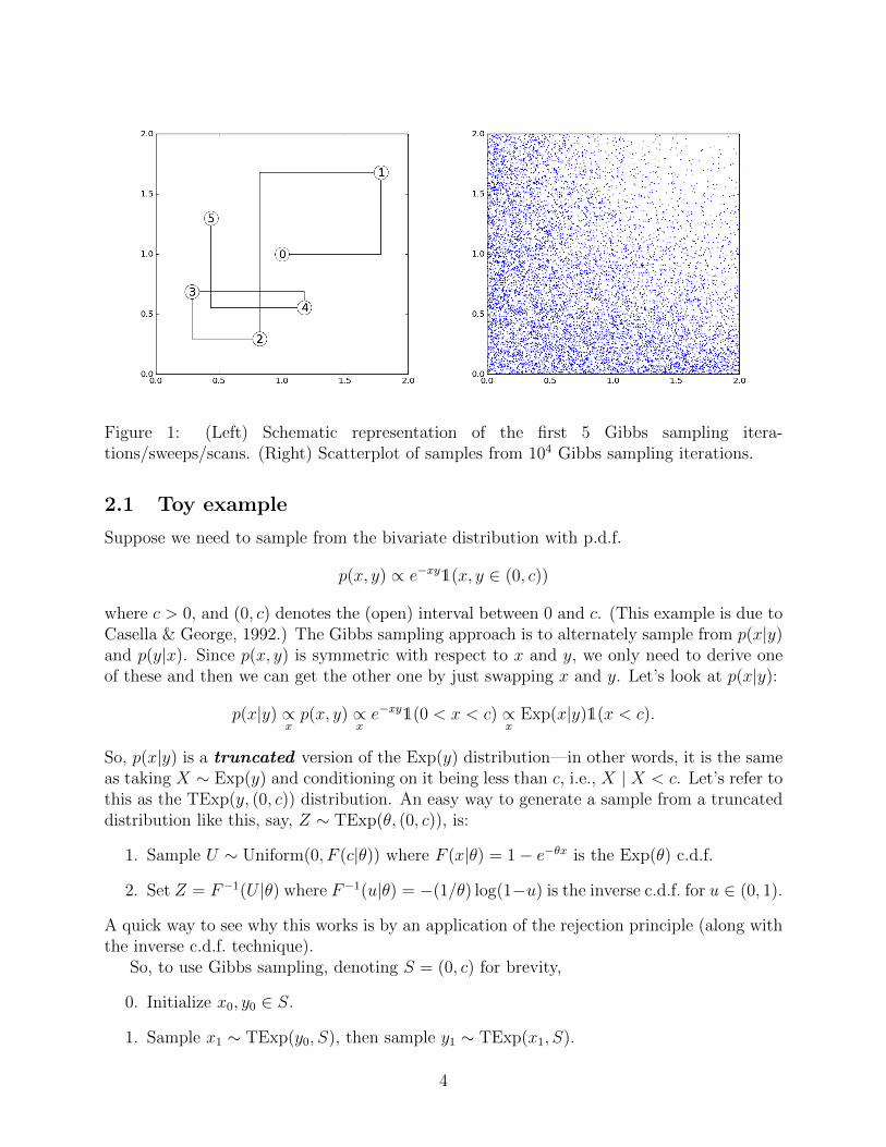
Figure 1: (Left) Schematic representation of the first 5 Gibbs sampling itera-tions/sweeps/scans. (Right) Scatterplot of samples from 104 Gibbs sampling iterations.

2.1 Toy example

Suppose we need to sample from the bivariate distribution with p.d.f.

p(x, y) ∝ e−xy1(x, y ∈ (0, c))

where c > 0, and (0, c) denotes the (open) interval between 0 and c. (This example is due toCasella & George, 1992.) The Gibbs sampling approach is to alternately sample from p(x|y)and p(y|x). Since p(x, y) is symmetric with respect to x and y, we only need to derive oneof these and then we can get the other one by just swapping x and y. Let’s look at p(x|y):

p(x|y) ∝xp(x, y) ∝

xe−xy1(0 < x < c) ∝

xExp(x|y)1(x < c).

So, p(x|y) is a truncated version of the Exp(y) distribution—in other words, it is the sameas taking X ∼ Exp(y) and conditioning on it being less than c, i.e., X | X < c. Let’s refer tothis as the TExp(y, (0, c)) distribution. An easy way to generate a sample from a truncateddistribution like this, say, Z ∼ TExp(θ, (0, c)), is:

1. Sample U ∼ Uniform(0, F (c|θ)) where F (x|θ) = 1− e−θx is the Exp(θ) c.d.f.

2. Set Z = F−1(U |θ) where F−1(u|θ) = −(1/θ) log(1−u) is the inverse c.d.f. for u ∈ (0, 1).

A quick way to see why this works is by an application of the rejection principle (along withthe inverse c.d.f. technique).

So, to use Gibbs sampling, denoting S = (0, c) for brevity,

0. Initialize x0, y0 ∈ S.

1. Sample x1 ∼ TExp(y0, S), then sample y1 ∼ TExp(x1, S).

4

2. Sample x2 ∼ TExp(y1, S), then sample y2 ∼ TExp(x2, S)....

N . Sample xN ∼ TExp(yN−1, S), then sample yN ∼ TExp(xN , S).

Figure 1 demonstrates the algorithm, with c = 2 and initial point (x0, y0) = (1, 1).

2.2 Example: Normal with semi-conjugate prior

In Chapter 4, we considered a conjugate prior for the mean µ and precision λ of a univariatenormal distribution, N (µ, λ−1), in which the variance of µ|λ depended on λ. However, it isoften more realistic to use independent priors on µ and λ, since we often don’t expect themean to be informative about the precision, or vice versa. In particular, consider the priorin which we take

µ ∼ N (µ0, λ−10 )

λ ∼ Gamma(a, b)

independently, and suppose X1, . . . , Xn|µ, λiid∼ N (µ, λ−1) as usual. Unfortunately, this is

not a conjugate prior. Nonetheless, it is semi-conjugate in the sense that the prior on µis conjugate for each fixed value of λ, and the prior on λ is conjugate for each fixed value ofµ. From our study of the Normal–Normal model, we know that for any fixed value of λ,

µ|λ, x1:n ∼ N (Mλ, L−1λ )

i.e., p(µ|λ, x1:n) = N (µ |Mλ, L−1λ ), where Lλ = λ0 + nλ and

Mλ =λ0µ0 + λ

∑ni=1 xi

λ0 + nλ.

Meanwhile, for any fixed value of µ, it is straightforward to derive (see Appendix) that

λ|µ, x1:n ∼ Gamma(Aµ, Bµ) (2.1)

where Aµ = a+ n/2 and

Bµ = b+ 12

∑(xi − µ)2 = nσ̂2 + n(x̄− µ)2

where σ̂2 = 1n

∑(xi − x̄)2.

So, to implement Gibbs sampling in this example, each iteration would consist of sampling

µ|λ, x1:n ∼ N (Mλ, L−1λ )

λ|µ, x1:n ∼ Gamma(Aµ, Bµ).

5

2.3 Example: Pareto model

Distributions of sizes and frequencies often tend to follow a “power law” distribution. Hereare a few examples of data which have been claimed to follow this type of distribution:

• wealth of individuals

• size of oil reserves

• size of cities

• word frequency

• returns on stocks

• size of meteorites

The Pareto distribution with shape α > 0 and scale c > 0 has p.d.f.

Pareto(x|α, c) =αcα

xα+11(x > c) ∝ 1

xα+11(x > c).

This is referred to as a power law distribution, because the p.d.f. is proportional to x raisedto a power. Notice that c is a lower bound on the observed values. In this example, we’ll seehow Gibbs sampling can be used to perform inference for α and c.

Table 1 shows the populations of the 50 largest cities in the state of North Carolina,according to the 2010 census.1 The Pareto distribution is often a good model for this typeof data.

2.3.1 Model

Let’s use a Pareto model for this population data:

X1, . . . , Xn|α, ciid∼ Pareto(α, c)

where Xi is the population of city i.

Reader: Now hold on just one second. You’re going to treat the 50 largest cities asa random sample? That seems fishy.

Author: Why?

Reader: Well, clearly there is selection bias here, because you are only looking at thelargest cities.

Author: Good grief, you’re right! Hmm, let’s see. . .

Reader: Oh, wait—it doesn’t matter!

Author: Huh, why?

1http://en.wikipedia.org/wiki/List_of_municipalities_in_North_Carolina

6

Rank City Population

1 Charlotte 7314242 Raleigh 4038923 Greensboro 2696664 Durham 2283305 Winston-Salem 2296186 Fayetteville 2005647 Cary 1352348 Wilmington 1064769 High Point 10437110 Greenville 8455411 Asheville 8571212 Concord 7906613 Gastonia 7174114 Jacksonville 7014515 Chapel Hill 5723316 Rocky Mount 5747717 Burlington 4996318 Huntersville 4677319 Wilson 4916720 Kannapolis 4262521 Apex 3747622 Hickory 4001023 Goldsboro 3643724 Indian Trail 3351825 Mooresville 32711

26 Wake Forest 3011727 Monroe 3279728 Salisbury 3362229 New Bern 2952430 Sanford 2809431 Matthews 2719832 Holly Springs 2466133 Thomasville 2675734 Cornelius 2486635 Garner 2574536 Asheboro 2501237 Statesville 2453238 Mint Hill 2272239 Kernersville 2312340 Morrisville 1857641 Lumberton 2154242 Kinston 2167743 Fuquay-Varina 1793744 Havelock 2073545 Carrboro 1958246 Shelby 2032347 Clemmons 1862748 Lexington 1893149 Elizabeth City 1868350 Boone 17122

Table 1: Populations of the 50 largest cities in the state of North Carolina, USA.

7

Reader: Because using only the largest cities is essentially like “rejecting” all thecities below some cutoff point c, and by the rejection principle, the remainingsamples are distributed according to the conditional distribution given x >c. And if the original data was Pareto(x|α, c0) for some c0 < c, then theconditional distribution given x > c is Pareto(x|α, c), because

Pareto(x|α, c0)1(x > c) ∝ Pareto(x|α, c).

Author: Oh, cool! So, our inferences regarding α will be valid, but c is essentiallyjust determining this cutoff point.

Reader: Right. OK, good.

In this example, the parameters have the following interpretation:

• α tells us the scaling relationship between the size of cities and their probability ofoccurring. For instance, if α = 1 then the density looks like 1/xα+1 = 1/x2, so citieswith 10,000–20,000 inhabitants occur roughly 10α+1 = 100 times as frequently as citieswith 100,000–110,000 inhabitants (or 10α+1/10 = 10 times as frequently as cities with100,000–200,000 inhabitants).

• c represents the cutoff point—any cities smaller than this were not included in thedataset.

To keep things as simple as possible, let’s use an (improper) flat prior:

p(α, c) ∝ 1(α, c > 0).

An improper prior is a nonnegative function of the parameters which integrates to infinity,so it can’t really be considered to define a prior distribution. But, we can still plug it intoBayes’ formula, and often (but not always!) the resulting “posterior” will be proper—in otherwords, the likelihood times the prior integrates to a finite value, and so this “posterior” is awell-defined a probability distribution. It is important that the “posterior” be proper, sinceotherwise the whole Bayesian framework breaks down. Improper priors are often used in anattempt to make a prior as non-informative as possible, in other words, to represent aslittle prior knowledge as possible. They are sometimes also mathematically convenient.

2.3.2 Posterior

So, plugging these into Bayes’ theorem, we define the posterior to be proportional to thelikelihood times the prior:

p(α, c|x1:n)def∝α,cp(x1:n|α, c)p(α, c)

∝α,c

1(α, c > 0)n∏i=1

αcα

xα+1i

1(xi > c)

=αncnα

(∏xi)α+1

1(c < x∗)1(α, c > 0) (2.2)

8

where x∗ = min{x1, . . . , xn}. As a joint distribution on (α, c), this does not seem to have arecognizable form, and it is not clear how we might sample from it directly. Let’s try Gibbssampling! To use Gibbs, we need to be able to sample α|c, x1:n and c|α, x1:n. By Equation2.2, we find that

p(α|c, x1:n) ∝αp(α, c|x1:n) ∝

α

αncnα

(∏xi)α

1(α > 0)

= αn exp(− α(

∑log xi − n log c)

)1(α > 0)

∝α

Gamma(α∣∣n+ 1,

∑log xi − n log c

),

and

p(c|α, x1:n) ∝cp(α, c|x1:n) ∝

ccnα1(0 < c < x∗).

Reader: I don’t recognize the form of this distribution on c.

Author: Me neither, but it looks nice and simple!

Reader: Totally. It should be a piece of cake to compute the normalizing constant.

Author: Yep, and I bet the c.d.f. will be simple enough that we can use the inversec.d.f. method to sample from it.

Reader: Let’s try it.

2.3.3 Sampling c using the inverse c.d.f. technique

For a > 0 and b > 0, define the distribution Mono(a, b) (for monomial) with p.d.f.

Mono(x|a, b) ∝ xa−11(0 < x < b).

Since∫ b0xa−1dx = ba/a, we have

Mono(x|a, b) =a

baxa−11(0 < x < b),

and for 0 < x < b, the c.d.f. is

F (x|a, b) =

∫ x

0

Mono(y|a, b)dy =a

baxa

a=xa

ba.

To use the inverse c.d.f. technique, we solve for the inverse of F on 0 < x < b:

u =xa

ba

bau = xa

bu1/a = x

and thus, we can sample from Mono(a, b) by drawing U ∼ Uniform(0, 1) and setting X =bU1/a. (By the way, it turns out that this is an inverse of the Pareto distribution, in the sensethat if X ∼ Pareto(α, c) then 1/X ∼ Mono(α, 1/c), and vice versa, but for the purposes ofthis example, I assumed that this was not known.)

9

2.3.4 Results

So, in order to use the Gibbs sampling algorithm to sample from the posterior p(α, c|x1:n),we initialize α and c, and then alternately update them by sampling:

α|c, x1:n ∼ Gamma(n+ 1,

∑log xi − n log c

)c|α, x1:n ∼ Mono(nα + 1, x∗).

Initializing at α = 1 and c = 100, we run the Gibbs sampler for N = 103 iterations onthe 50 data points from Table 1, giving us a sequence of samples

(α1, c1), . . . , (αN , cN).

Figure 2 shows various ways of viewing the results.

(a) Traceplots. A traceplot simply shows the sequence of samples, for instanceα1, . . . , αN , or c1, . . . , cN . Traceplots are a simple but very useful way to visualizehow the sampler is behaving. The traceplots in Figure 2(a) look very healthy—thesampler doesn’t appear to be getting stuck anywhere.

(b) Scatterplot. The scatterplot in panel (b) shows us what the posterior distributionp(α, c|x1:n) looks like. The smallest city in our data set is Boone, with a population of17,122, and the posterior on c is quite concentrated just under this value, which makessense since c represents the cutoff point in the sampling process.

(c) Estimated density. We are primarily interested in the posterior on α, since it tells usthe scaling relationship between the size of cities and their probability of occurring. Bymaking a histogram of the samples α1, . . . , αN , we can estimate the posterior densityp(α|x1:n). The two vertical lines indicate the lower ` and upper u boundaries of an(approximate) 90% credible interval [`, u]—that is, an interval that contains 90% ofthe posterior probability:

P(α ∈ [`, u]

∣∣x1:n) = 0.9.

The interval shown here is approximate since it’s based on the samples. This can becomputed from the samples by sorting them α(1) ≤ · · · ≤ α(N) and setting

` = α(b0.05Nc) u = α(d0.95Ne)

where bxc and dxe are the floor and ceiling functions, respectively.

(d) Running averages. Panel (d) shows the running average 1k

∑ki=1 αi for k = 1, . . . , N .

In addition to traceplots, running averages such as this are a useful heuristic for visuallyassessing the convergence of the Markov chain. The running average shown in thisexample still seems to be meandering about a bit, suggesting that the sampler needsto be run longer (but this would depend on the level of accuracy desired).

(e) Panel (e) is particular to this example. Power law distributions are often displayed byplotting their survival function S(x)—that is, one minus the c.d.f., S(x) = P(X > x) =1− P(X ≤ x)—on a log-log plot, since S(x) = (c/x)α for the Pareto(α, c) distribution

10

(a) Traceplots of α (top) and c (bottom).

(b) Scatterplot of samples. (c) Estimated density of α|x1:n.

(d) 1k

∑ki=1 αi for k = 1, . . . , N . (e) Empirical vs posterior survival function.

Figure 2: Results from the power law example.

11

and on a log-log plot this appears as a line with slope −α. The posterior survivalfunction (or more precisely, the posterior predictive survival function), is S(x|x1:n) =P(Xn+1 > x | x1:n). Figure 2(e) shows an empirical estimate of the survival function(based on the empirical c.d.f., F̂ (x) = 1

n

∑ni=1 1(x ≥ xi)) along with the posterior

survival function, approximated by

S(x|x1:n) = P(Xn+1 > x | x1:n) =

∫P(Xn+1 > x | α, c)p(α, c|x1:n)dαdc

≈ 1

N

N∑i=1

P(Xn+1 > x | αi, ci) =1

N

N∑i=1

(ci/x)αi .

This is computed for each x in a grid of values.

It is important to note that even when heuristics like traceplots and running averages appearto indicate that all is well, it is possible that things are going horribly wrong. For instance,it is not uncommon for there to be multiple modes, and for the sampler to get stuck in oneof them for many iterations.

3 Gibbs sampling with more than two variables

In Section 2, we saw how to use Gibbs sampling for distributions with two variables, e.g.,p(x, y). The generalization to more than two variables is completely straightforward—roughly speaking, we cycle through the variables, sampling each from its conditional dis-tributional given all the rest.

For instance, for a distribution with three random variables, say, p(x, y, z), we set x, y,and z to some initial values, and then sample x|y, z, then y|x, z, then z|x, y, then x|y, z, andso on. More precisely,

0. Set (x0, y0, z0) to some starting value.

1. Sample x1 ∼ p(x|y0, z0).Sample y1 ∼ p(y|x1, z0).Sample z1 ∼ p(z|x1, y1).

2. Sample x2 ∼ p(x|y1, z1).Sample y2 ∼ p(y|x2, z1).Sample z2 ∼ p(z|x2, y2)....

In general, for distribution with d random variables, say, p(v1, . . . , vd), at each iterationof the algorithm, we sample from

v1 | v2, v3, . . . , vd

v2 | v1, v3, . . . , vd...

vd | v1, v2, . . . , vd−1

12

always using the most recent values of all the other variables. The conditional distributionof a variable given all of the others is sometimes referred to as the full conditional in thiscontext, and for brevity this is sometimes denoted vi| · · · .

3.1 Example: Censored data

In many real-world data sets, some of the data is either missing altogether or is partiallyobscured. Gibbs sampling provides a method for dealing with these situations in a completelycoherent Bayesian way, by sampling these missing variables along with the parameters. Thisalso provides information about the values of the missing/obscured data.

One way in which data can be partially obscured is by censoring, which means that weknow a data point lies in some particular interval, but we don’t get to observe it exactly.Censored data occurs very frequently in medical research such as clinical trials (since forinstance, the researchers may lose contact with some of the patients), and also in engineering(since some measurements may exceed the lower or upper limits of the instrument beingused).

To illustrate, suppose researchers are studying the length of life (lifetime) following aparticular medical intervention, such as a new surgical treatment for heart disease, and in astudy of 12 patients, the number of years before death for each is

3.4, 2.9, 1.2+, 1.4, 3.2, 1.8, 4.6, 1.7+, 2.0+, 1.4+, 2.8, 0.6+

where x+ indicates that the patient was alive after x years, but the researchers lost contactwith the patient at that point. (Of course, there will always also be a control group, butlet’s focus on one group to keep things simple.) Consider the following model:

θ ∼ Gamma(a, b)

Z1, . . . , Zn|θiid∼ Gamma(r, θ)

Xi =

{Zi if Zi ≤ ci∗ if Zi > ci.

where a, b, and r are known, and ∗ is a special value to indicate that censoring has occurred.The interpretation is:

• θ is the parameter of interest—the rate parameter for the lifetime distribution.

• Zi is the lifetime for patient i, however, this is not directly observed.

• ci is the censoring time for patient i, which is fixed, but known only if censoring occurs.

• Xi is the observation—if the lifetime is less than ci then we get to observe it (Xi = Zi),otherwise all we know is the lifetime is greater than ci (Xi = ∗).

3.1.1 The posterior is complicated

Unfortunately, the posterior p(θ|x1:n) ∝ p(x1:n|θ)p(θ) does not reduce to a simple form thatwe can easily work with. The reason is that the likelihood p(x1:n|θ) involves the distribution

13

of the observations xi given θ, integrating out the zi’s, and in the case of censored observationsxi = ∗, this is

p(xi|θ) = P(Xi = ∗ | θ) = P(Zi > c | θ),

which is one minus the Gamma(r, θ) c.d.f., a rather complicated function of θ.Also, p(z1:n|x1:n) (the posterior on the zi’s, with θ integrated out) looks a bit nasty as

well, and it’s not immediately clear to me how one would sample from it.

3.1.2 Gibbs sampling approach

Meanwhile, the Gibbs sampling approach is a cinch. To sample from p(θ, z1:n|x1:n), we cyclethrough each of the full conditional distributions,

θ | z1:n, x1:nz1 | θ, z2:n, x1:nz2 | θ, z1, z3:n, x1:n

...

zn | θ, z1:n−1, x1:n

sampling from each in turn, always conditioning on the most recent values of the othervariables. The full conditionals are easy to calculate:

• (θ| · · · ) Since θ ⊥ x1:n | z1:n (i.e., θ is conditionally independent of x1:n given z1:n),

p(θ| · · · ) = p(θ|z1:n, x1:n) = p(θ|z1:n) = Gamma(θ∣∣ a+ nr, b+

∑ni=1 zi

)using the fact that the prior on θ is conjugate. (See Exercise 3 of Chapter 3.)

• (zi| · · · ) If xi 6= ∗ then zi is forced to be equal to xi. Otherwise,

p(zi| · · · ) = p(zi|θ, z(1:n)−i, x1:n) = p(zi|θ, xi)∝zip(xi, zi|θ) = p(xi|zi)p(zi|θ)

= 1(zi > ci) Gamma(zi | r, θ)∝zi

TGamma(zi | r, θ, (ci,∞))

where TGamma(zi | r, θ, S) is the truncated Gamma distribution—that is, the distri-bution of a Gamma(r, θ) random variable conditioned on being in the set S.

We can sample from TGamma(r, θ, (c,∞)) with the same approach we used for the truncatedexponential in Section 2.1: if F (x|r, θ) denotes the Gamma(r, θ) c.d.f., then to draw a sampleZ ∼ TGamma(r, θ, (c,∞)),

1. sample U ∼ Uniform(F (c|r, θ), 1), and

2. set Z = F−1(U |r, θ).

14

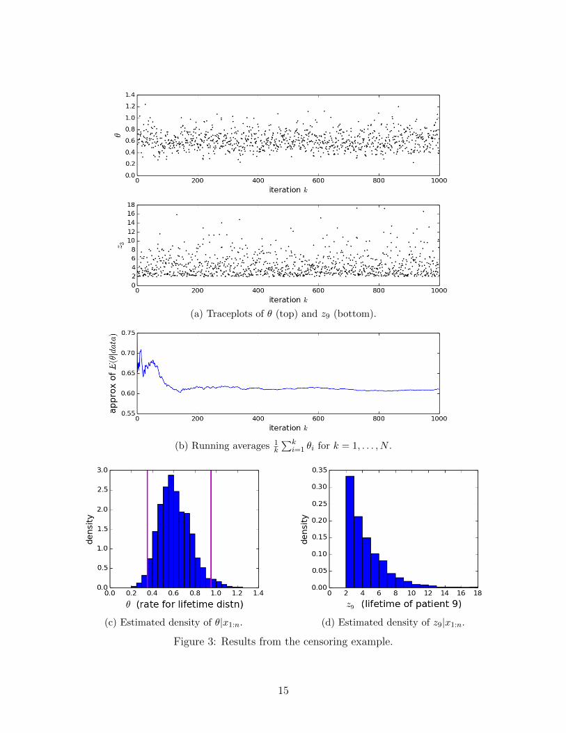
(a) Traceplots of θ (top) and z9 (bottom).

(b) Running averages 1k

∑ki=1 θi for k = 1, . . . , N .

(c) Estimated density of θ|x1:n. (d) Estimated density of z9|x1:n.

Figure 3: Results from the censoring example.

15

3.1.3 Results

Let’s suppose a = b = 1 and r = 2.0, and run the Gibbs sampler for N = 103 iterations,using initial values θ = 1 and zi = ci + 1 for those i’s that were censored. See Figure 3 forvarious traceplots, running averages, and estimated densities.

3.2 Example: Hyperpriors and hierarchical models

Gibbs sampling is spectacularly useful for models involving multiple levels, particularly wheneach piece of the model involves a conjugate (or at least semi-conjugate) prior. For instance,we may want to put a prior not only on the parameters, but also on the hyperparameters—that is, the parameters of the prior—this is called a hyperprior. This comes up particularlyoften when constructing hierarchical models, that is, models in which there is a hierar-chical structure to the relationships between the data, latent variables, and parameters.

As a simple example, consider the Normal model with semi-conjugate prior from Section2.2. Let’s put a Gamma(r, s) hyperprior on λ0, so that the model is now:

λ0 ∼ Gamma(r, s)

µ|λ0 ∼ N (µ0, λ−10 )

λ ∼ Gamma(a, b)

X1, . . . , Xn|λ0, µ, λ ∼ N (µ, λ−1).

You might recognize that this is equivalent to putting a t-distribution prior on µ. Sincethe t-distribution is not a conjugate prior for the mean of Normally-distributed data, wewould not be able to sample directly from µ|λ, x1:n. However, we can easily sample fromµ|λ0, λ, x1:n, and this is what we need for Gibbs sampling.

3.2.1 Gibbs sampler

• (λ0| · · · ) Since λ0 is conditionally independent of everything else given µ, this is exactlythe same as the posterior on the precision in a semi-conjugate Normal model with onedatapoint (namely, µ). Thus,

λ0|µ, λ, x1:n ∼ Gamma(r + 1/2, s+ 1

2(µ− µ0)

2).

• (µ| · · · ) Since we are conditioning on λ0, we are just in the usual situation for thesemi-conjugate Normal model without a hyperprior, and thus, just like in Section 2.2,

µ|λ0, λ, x1:n ∼ N (M,L−1)

where L = λ0 + nλ and M = (λ0µ0 + λ∑xi)/(λ0 + nλ).

• (λ| · · · ) We are again just in the usual situation for the semi-conjugate Normal, andthus

λ|λ0, µ, x1:n ∼ Gamma(A,B)

where A = a+ n/2 and B = nσ̂2 + n(x̄− µ)2.

16

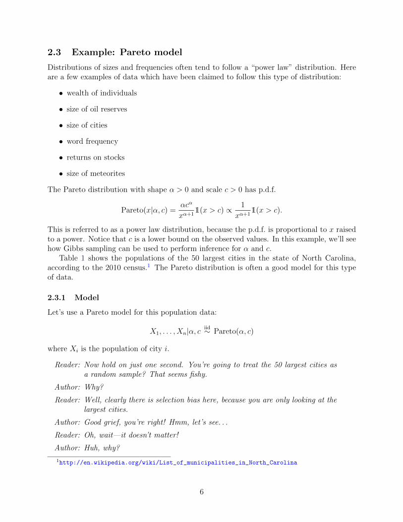
Figure 4: Heights of Dutch women and men, combined.

Each iteration of Gibbs sampling proceeds by sampling from each of these, in turn.We could just as easily put (semi-)conjugate priors on µ0 and b as well (specifically,

a Normal prior on µ0 and a Gamma prior on b), and include them as well in the Gibbssampling algorithm. In this simple example, these hyperpriors essentially just make theprior less informative, however, when constructing hierarchical models involving multiplegroups of datapoints, this approach can enable the “sharing of statistical strength” acrossgroups—roughly, using information learned from one group to help make inferences aboutthe others.

3.3 Example: Data augmentation / Auxiliary variables

A commonly-used technique for designing MCMC samplers is to use data augmentation,also known as auxiliary variables. The idea is to introduce a new variable (or variables)Z that depends on the distribution of the existing variables in such a way that the resultingconditional distributions, with Z included, are easier to sample from and/or result in bettermixing (faster convergence). So, the Z’s are essentially latent/hidden variables that areintroduced for the purpose of simplifying/improving the sampler. For instance, suppose wewant to sample from p(x, y), but p(x|y) and/or p(y|x) are complicated. If we can choosesome p(z|x, y) such that p(x|y, z), p(y|x, z), and p(z|x, y) are easy to sample from, then wecan construct a Gibbs sampler to sample all three variables (X, Y, Z) from p(x, y, z) andthen just throw away the Z’s and we will have samples (X, Y ) from p(x, y).

To illustrate, consider the data set from Chapter 4 consisting of the heights of 695 Dutchwomen and 562 Dutch men. Suppose we have the list of heights, but we don’t know whichdatapoints are from women and which are from men. See Figure 4. Can we still inferthe distribution of female heights and male heights, e.g., the mean for males and the meanfor females? Perhaps surprisingly, the answer is yes. The reason is that this is a two-component mixture of Normals, and there is an (essentially) unique set of mixture parameterscorresponding to any such distribution.

To construct a Gibbs sampler for a mixture model such as this, it is common to introduce

17

an auxiliary variable Zi for each datapoint, indicating which mixture component it is drawnfrom. For instance, in this example, Zi would indicate whether subject i is female or male.This results in a Gibbs sampler that is quite easy to derive and implement.

3.3.1 Two-component mixture model

To keep things as simple as possible, let’s assume that both mixture components (femaleand male) have the same precision (inverse variance), say λ, and that λ is fixed and known.Then the usual two-component Normal mixture model is:

µ0, µ1iid∼ N (m, `−1)

π ∼ Beta(a, b)

X1, . . . , Xn|µ, πiid∼ F (µ, π)

where F (µ, π) is the distribution with p.d.f.

f(x|µ, π) = (1− π)N (x | µ0, λ−1) + πN (x | µ1, λ

−1)

and µ = (µ0, µ1).The likelihood is

p(x1:n|µ, π) =n∏i=1

f(xi|µ, π)

=n∏i=1

[(1− π)N (xi | µ0, λ

−1) + πN (xi | µ1, λ−1)]

which is a complicated function of µ and π, making the posterior difficult to sample fromdirectly.

3.3.2 Allocation variables to the rescue

We can define an equivalent model that includes latent “allocation” variables Z1, . . . , Zn toindicate which mixture component each datapoint comes from—that is, Zi indicates whethersubject i is female or male.

µ0, µ1iid∼ N (m, `−1)

π ∼ Beta(a, b)

Z1, . . . , Zn|µ, πiid∼ Bernoulli(π)

Xi ∼ N (µZi, λ−1) independently for i = 1, . . . , n.

This is equivalent to the model above, since

p(xi|µ, π) = p(x|Zi = 0, µ, π)P(Zi = 0|µ, π) + p(x|Zi = 1, µ, π)P(Zi = 1|µ, π)

= (1− π)N (xi|µ0, λ−1) + πN (xi|µ1, λ

−1)

= f(xi|µ, π),

and thus it induces the same distribution on (x1:n, µ, π). However, it is considerably easierto work with, particularly for Gibbs sampling.

18

3.3.3 Gibbs sampling

We derive the full conditionals. For brevity, denote x = x1:n and z = z1:n.

• (π| · · · ) Given z, π is independent of everything else, so this reduces to a Beta–Bernoullimodel, and we have

p(π|µ, z, x) = p(π|z) = Beta(π | a+ n1, b+ n0)

where nk =∑n

i=1 1(zi = k) for k ∈ {0, 1}.

• (µ| · · · ) Given z, we know which component each datapoint comes from , so the model(conditionally on z) is just two independent Normal–Normal models, and thus (like inSection 2.2):

µ0|µ1, x, z, π ∼ N (M0, L−10 )

µ1|µ0, x, z, π ∼ N (M1, L−11 )

where for k ∈ {0, 1},

nk =n∑i=1

1(zi = k)

Lk = `+ nkλ

Mk =`m+ λ

∑i:zi=k

xi

`+ nkλ.

• (z| · · · )

p(z|µ, π, x) ∝zp(x, z, π, µ) ∝

zp(x|z, µ)p(z|π)

=n∏i=1

N (xi|µzi , λ−1) Bernoulli(zi|π)

=n∏i=1

(πN (xi|µ1, λ

−1))zi(

(1− π)N (xi|µ0, λ−1))1−zi

=n∏i=1

αzii,1α1−zii,0

∝z

n∏i=1

Bernoulli(zi | αi,1/(αi,0 + αi,1))

where

αi,0 = (1− π)N (xi|µ0, λ−1)

αi,1 = πN (xi|µ1, λ−1).

As usual, each iteration of Gibbs sampling proceeds by sampling from each of these condi-tional distributions, in turn.

19

(a) Traceplots of the component means, µ0 and µ1.

(b) Traceplot of the mixture weight, π (prior probability that a subject comes from component 1).

(c) Histograms of the heights of subjects assigned to each component, according to z1, . . . , zn, in atypical sample.

Figure 5: Results from one run of the mixture example.

20

3.3.4 Results

We implement this Gibbs sampler with the following parameter settings:

• λ = 1/σ2 where σ = 8 cm (≈ 3.1 inches) (σ = standard deviation of the subject heightswithin each component)

• a = 1, b = 1 (Beta parameters, equivalent to prior “sample size” of 1 for each compo-nent)

• m = 175 cm (≈ 68.9 inches) (mean of the prior on the component means)

• ` = 1/s2 where s = 15 cm (≈ 6 inches) (s = standard deviation of the prior on thecomponent means)

We initialize the sampler at:

• π = 1/2 (equal probability for each component)

• z1, . . . , zn sampled i.i.d. from Bernoulli(1/2) (initial assignment to components chosenuniformly at random)

• µ0 = µ1 = m (component means initialized to the mean of their prior)

Figure 5 shows a few plots of the results for N = 103 iterations. (Note: This should probablybe run for longer—this short run is simply for illustration purposes.) From the traceplots ofµ0 and µ1, we see that one component quickly settles to have a mean of around 168–170 cmand the other to a mean of around 182–186 cm. Recalling that we are not using the trueassignments of subjects to components (that is, we don’t know whether they are male orfemale), it is interesting to note that this is fairly close to the sample averages: 168.0 cm (5feet 6.1 inches) for females, and 181.4 cm (5 feet 11.4 inches) for males.

The traceplot of π indicates that the sampler is exploring values of around 0.2 to 0.4—thatis, the proportion of people coming from group 1 is around 0.2 to 0.4. Meanwhile, looking atthe actual labels (female and male), the empirical proportion of males is 562/(695 + 562) ≈0.45. So this is slightly off. This could be due to not having enough data, and/or due to thefact that we are assuming a fixed value of λ. It would be much better, and nearly as easy,to allow components 0 and 1 to have different precisions, λ0 and λ1, and put Gamma priorson them.

As shown in the bottom plot (panel (c)), one way of visualizing the allocation/assignmentvariables z1, . . . , zn is to make histograms of the heights of the subjects assigned to eachcomponent. At a glance, this shows us where the two clusters of datapoints are, how largeeach cluster is, and what shape they have.

3.3.5 A potentially serious issue: It’s not mixing!

This example illustrates one of the big things that can go wrong with MCMC (althoughfortunately, in this case, the results are still valid if interpreted correctly). Why are femalesassigned to component 0 and males assigned to component 1? Why not the other wayaround? In fact, the model is symmetric with respect to the two components, and thus the

21

(a) Traceplots of the component means, µ0 and µ1.

(b) Traceplot of the mixture weight, π (prior probability that a subject comes from component 1).

(c) Histograms of the heights of subjects assigned to each component, according to z1, . . . , zn, in atypical sample.

Figure 6: Results from another run of the mixture example.

22

posterior is also symmetric. If we run the sampler multiple times (starting from the sameinitial values), sometimes it will settle on females as 0 and males as 1, and sometimes onfemales as 1 and males as 0 — see Figure 6. Roughly speaking, the posterior has two modes.If the sampler were behaving properly, it would move back and forth between these twomodes, but it doesn’t—it gets stuck in one and stays there.

This is a very common problem with mixture models. Fortunately, however, in the caseof mixture models, the results are still valid if we interpret them correctly. Specifically, ourinferences will be valid as long as we only consider quantities that are invariant with respectto permutations of the components.

23

4 Exercises

1. Consider the bivariate distribution with p.d.f.

p(x, y) ∝ 1(|x− y| < c)1(x, y ∈ (0, 1)))

where (0, 1) denotes the (open) interval from 0 to 1.

(a) Derive the Gibbs sampler for this distribution (in this parametrization).

(b) Implement and run the Gibbs sampler for N = 103 iterations, for each of thefollowing: c = 0.25, c = 0.05, and c = 0.02.

(c) For each of these values of c, make a traceplot of x and a scatterplot of (x, y).

(d) Explain why the sampler will perform worse and worse as c gets smaller.

2. The issue with the sampler in Exercise 1 can be fixed using the following change ofvariables:

U =X + Y

2, V =

X − Y2

.

Using Jacobi’s formula for transformations of random variables, it can be shown (youare not required to show this for the exercise) that the p.d.f. of (U, V ) is

p(u, v) ∝ 1(|v| < c/2)1(|v| < u < 1− |v|).

Samples of (U, V ) can be transformed back into samples of (X, Y ) by the inversetransformation:

X = U + V, Y = U − V. (4.1)

Now using p(u, v), repeat parts (a), (b), and (c) from Exercise 1, except that in part(c), transform your (u, v) samples into (x, y) samples using Equation 4.1 before makingthe traceplots and scatterplots. Explain why this sampler does not suffer from the sameissue as the previous one. (Hint: You may find it helpful to draw a picture to figureout the conditional distributions u|v and v|u.)

3. (More to come. . . )

Supplementary material

• Hoff (2009), 6.

• mathematicalmonk videos, Machine Learning (ML) 18.1–18.9https://www.youtube.com/playlist?list=PLD0F06AA0D2E8FFBA

24

References

• S. Geman, and D. Geman. “Stochastic relaxation, Gibbs distributions, and theBayesian restoration of images.” Pattern Analysis and Machine Intelligence, IEEETransactions on 6 (1984): 721-741.

• G. Casella, and E.I. George. “Explaining the Gibbs sampler.” The American Statisti-cian 46.3 (1992): 167-174.

• A. Clauset, A., C.R. Shalizi, , and M.E.J. Newman. “Power-law distributions in em-pirical data.” SIAM review 51.4 (2009): 661-703.

Proofs

Conditional distribution of λ for semi-conjugate prior

We derive the distribution of λ given µ, x1:n, as in Equation 2.1:

p(λ|µ, x1:n) =p(λ, µ, x1:n)

p(µ, x1:n)

∝λp(λ, µ, x1:n)

= p(x1:n|µ, λ)p(µ)p(λ)

∝λp(λ)

n∏i=1

p(xi|µ, λ)

=ba

Γ(a)λa−1 exp(−bλ)

n∏i=1

√λ

2πexp

(− 1

2λ(xi − µ)2

)∝λλa+

n2−1 exp

(− λ[b+ 1

2

∑(xi − µ)tothepart2

])∝λ

Gamma(λ∣∣∣ a+ n/2, b+ 1

2

∑(xi − µ)2

)and ∑

(xi − µ)2 =∑

(xi − x̄+ x̄− µ)2

=∑[

(xi − x̄)2 + 2(xi − x̄)(x̄− µ) + (x̄− µ)2]

=∑

(xi − x̄)2 + 2(x̄− µ)∑

(xi − x̄) + n(x̄− µ)2

=∑

(xi − x̄)2 + n(x̄− µ)2

= nσ̂2 + n(x̄− µ)2.

25