Characteristics of resistance and velocity fil i d h l fl profiles in vegetated open channel flows

CHENG Nian-Shengg

S h l f Ci il d E i t l E i iSchool of Civil and Environmental EngineeringNanyang Technological University, Singapore

Hydraulics of Ve etated Open Channel Flo s Vegetated Open Channel Flows

• Experimental effortsExperimental efforts• Preliminary analyses

2

Research PurposeResearch Purpose

To study mean-flow and turbulence characteristics, and To study mean flow and turbulence characteristics, and sediment transportConditions: emergent and submerged vegetations Conditions: emergent and submerged vegetations Focus: shallow flows

3

Research Purpose (内幕)Research Purpose (内幕)

想歪了想歪了

走叉了走叉了

骑虎难下骑虎难下

4

Current status of the topic

It is hot, but Its understanding is limited

5

Unanswered questionsHow to evaluate flow resistance?

Does velocity profiles follow log‐law?

What is equivalent roughness height?

How about flow structures? 

How about turbulent diffusion?

How to compute sediment transport rates?rates?

6

Experiments conducted at NTU (2005-2012)

• Flume12 m long, 30 cm wide, 45 cm deepI di id l i l i• Individual circulating systems for water and sediment

7

Simulated rigid vegetation

Arrays of rigid rods planted at Perspex plates.Rod diameters: d = 3 mm 6 mm and 8 mm

g g

Rod diameters: d = 3 mm, 6 mm, and 8 mm

Varying distances between two neighboring rods

8

Bed configurationBed configuration

9

Flow sampling LDAFlow sampling LDA

Equipments employed:

EMCM

2D Laser Doppler Anemometry (LDA)

EMCM

2D Electromagnetic Current M (EMCM)Meter (EMCM)

2D P i l I V l i

PIV

2D Particle Image Velocimetry (PIV)

10

Basic profiles

Mean-velocity profiles

180

200B30 - Velocity profile

120

140

160

180

60

80

100

z (m

m)

H = 10 CM

H = 13 CM

H = 15 CM

0

20

40

0 0 1 0 2 0 3 0 4

H = 17 CM

H = 20 CM

0 0.1 0.2 0.3 0.4u (m/s)

Flow velocity profile for case B30

11

PIV-measured streamwise flow velocity

12

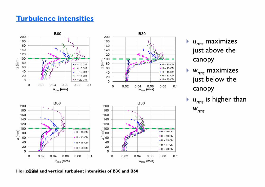
Turbulence intensities

urms maximizes just above the just above the canopywrms maximizes wrms maximizes just below the canopyurms is higher than wrms

Horizontal and vertical turbulent intensities of B30 and B6013

Completed analyses

1. Flow resistance for the emergent case2. Representative roughness height of submerged vegetation3. Scaling law for velocity profiles for the submerged case

d b d h f d fl d4. Drag prediction based on the concept of pseudo‐fluid

14

Analysis No. 1

Length Scale for Evaluating Resistance I d d b Si l d E V iInduced by Simulated Emergent Vegetation in Open Channel Flows

15

Definitions of Re for Open Channel Flows subject to Emergent VegetationEmergent Vegetation

Investigator  Reynolds number

Characteristic velocity

Characteristic lengthnumber velocity  length

Wu et al. (1999)  Vhν

 bulk velocity, V  flow depth, h

νIshikawa et al. (2000) 

Vdν

 bulk velocity, V  stem diameter, d

Lee et al. (2004)  Vhν

; Vsν

; bulk velocity, V  flow depth, h;

stem spacing, s; stem diameter dVd

ν 

stem diameter, d

i d f d h i i lTanino and Nepf (2008) 

vV dν

 average pore velocity among stems, Vv  

characteristic plant width or stem diameter, d

K h i l

16

, v

 ,

Kothyari et al. (2009) 

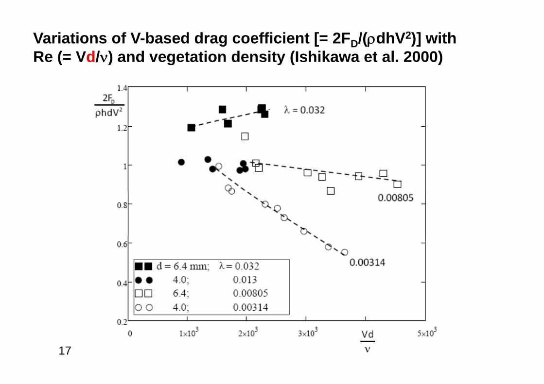
Variations of V-based drag coefficient [= 2FD/(ρdhV2)] with Re (= Vd/ν) and vegetation density (Ishikawa et al. 2000)Re ( Vd/ν) and vegetation density (Ishikawa et al. 2000)

17

Dependence of Vv-based drag coefficient [= 2FD/(ρdhVv2)] on

Re (= V d/ν) and vegetation density (Kothyari et al 2009)Re ( Vvd/ν) and vegetation density (Kothyari et al. 2009)

18

Linear dependence of normalized drag (0.5CDvVvd/ν) R ( V d/ ) (T i d N f 2008)on Re (=Vvd/ν) (Tanino and Nepf, 2008)

19

Definition: Vegetation-Related Hydraulic Radius

Φ f = fluid-occupied volumef pA v = frontal area of stems

Hydraulic radius：

f (1 )h 1Φ − λ π − λ

Hydraulic radius：

f vv

v v

(1 )h 1r d

A 4 h / ( d) 4Φ λ π λ

= = =λ π λ

20

Definition: Vegetation-Related Hydraulic Radius

1π − λv

1r d

4π λ

=λ

vv 2

8gr Sf

V= v v

v

4V rRe =

νvV ν

( )v vf f Re=21

( )v v

Drag coefficient

2vVF C hd

g ff

vD DvF C hd

2= ρ

2 2v v

D Dv Dv2

V 2 hV4NF C hd C

d 2 dλρλ

= ρ =π πd 2 dπ π

2v2 hV

C (1 ) ghSλρ

λvDvC (1 ) ghS

dρ

= − λ ρπ

Dv v

1C f= ( )f Re=

22

Dv v4( )vf Re

Dependence of drag coefficient [CDv = 2FD/(ρhdVv2)] on

Re (=4V r /ν) The data are from Kothyari et al (2009)Rev ( 4Vvrv/ν). The data are from Kothyari et al. (2009)

Original graphImproved data collapse

CDv

Original graphp p

Dv

Rev

23

Dependence of drag coefficient [CDv = 2FD/(ρhdVv2)] on

Re (= 4V r /ν) The data points are from Ishikawa et al (2000)Re (= 4Vvrv/ν). The data points are from Ishikawa et al. (2000)

Original graphImproved data collapse

CDv

Rev

24

Dependence of drag coefficient [CDv = 2FD/(ρhdVv2)] on

Re (= 4V r /ν) The data are from Tanino and Nepf (2008)Rev ( 4Vvrv/ν). The data are from Tanino and Nepf (2008)

Original graphImproved data collapse

CDv

Original graphp p

Dv

Rev

25

CDv

26 Rev

CCDv

27Rev

Use of d rather than rv

28

Calculation of Manning’s n

29

30

Conclusion from Analysis No. 1Conclusion from Analysis No. 1

Q i H i fl iQuestion: How to estimate flow resistance for emergent case?gPossible answer: To apply the concept of hydraulic radius to the flow throughhydraulic radius to the flow through vegetation.

Ref: Cheng, N. S. and Nguyen, H. T. (2010). “Hydraulic radius for g g y ( ) yevaluating resistance induced by simulated emergent vegetation in open channel flows.” Journal of Hydraulic Engineering, ASCE. doi:10.1061/(ASCE)HY.1943-7900.0000377doi:10.1061/(ASCE)HY.1943 7900.0000377

Analysis No. 2

Representative roughness height f th f b d t tifor the case of submerged vegetation

32

Available length scales of roughness elements

Vegetation heightVegetation spacingVegetation diameter sVegetation diameter

dd

hv

33

hv

10

Entire flow

1

fEntire flow

1

0.1

Shi i l (1991)

0 01

Shimizu et al (1991)Dunn et al (1996)Meijer & van Velzen (1999) Stone & Shen (2002)Murphy et al (2007)hs y 0.01 p y ( )Yan (2008)Yang (2008) Liu et al (2008)Nezu & Sanjou (2008) P i t l (2009)

s y

0.1 1 101 10 3−×

Poggi et al (2009)Present study

h /r

hv

34

hv/r

10Shimizu et al (1991)Dunn et al (1996)Surface layer

1

Meijer & van Velzen (1999) Stone & Shen (2002)Murphy et al (2007)Yan (2008)Yang (2008)

Surface layeronly

1 Yang (2008) Liu et al (2008)Nezu & Sanjou (2008) Poggi et al (2009)Present study

fs

0.1

0 01hs y 0.01s y

0.1 1 10 1001 10 3−×

h /h

hv

35

hv/hs

10

Surface layer only

1

10

f

0.1

1fs

0.01 Shimizu et al (1991)

1 10 3−×

( )Dunn et al (1996)Meijer & van Velzen (1999) Stone & Shen (2002)Murphy et al (2007)

1 10 4−×

Yan (2008)Yang (2008) Liu et al (2008)Nezu & Sanjou (2008) Poggi et al (2009)

1 10 5−× 1 10 4−× 1 10 3−× 0.01 0.11 10 5−×

Poggi et al (2009)Present studyEquation (15)

k /h36

kv/hs

Conceptual ConsiderationConceptual Consideration

To quantify the linear size of flow domain, weTo quantify the linear size of flow domain, we use length scale - hydraulic radius

f vv

(1 )h 1r d

A 4 h / ( d) 4Φ − λ π − λ

= = =λ λv

v vA 4 h / ( d) 4λ π λ

Φf = fluid-occupied volumeA f t l f tA v = frontal area of stems

37

Roughness length scaleg g

To quantify how rough the stems are w r t theTo quantify how rough the stems are w.r.t the fluid-occupied volume,

v vv

hk d

Φ λ π λ= = =v

f vA 4(1 )h / ( d) 4 1− λ π − λ

Φv = vegetation-occupied volumev g pA f = equivalent frontal area for fluid-occupied

volume38

volume

frΦ

= vkΦ

vv

rA

= vv

f

kA

=

β⎛ ⎞k⎛ ⎞

= α⎜ ⎟⎝ ⎠

vs

kf

hα = 0.4; β = 1/8

10

⎝ ⎠sh

0 1

1

fs

0.01

0.1

Shimizu et al (1991)D t l (1996)

s

1 10 3−×

Dunn et al (1996)Meijer & van Velzen (1999) Stone & Shen (2002)Murphy et al (2007)Yan (2008)Y (2008)

1 10 4−×

Yang (2008) Liu et al (2008)Nezu & Sanjou (2008) Poggi et al (2009)Present studyEquation (15)

401 10 5−× 1 10 4−× 1 10 3−× 0.01 0.1

1 10 5−×

Equation (15)

kv/hs

Average flow velocity in the surface layer

λ⎛ ⎞1/16

1 h− λ⎛ ⎞= η⎜ ⎟λ⎝ ⎠s

s s

1 hU gh S

dλ⎝ ⎠d

η = 4.54

41

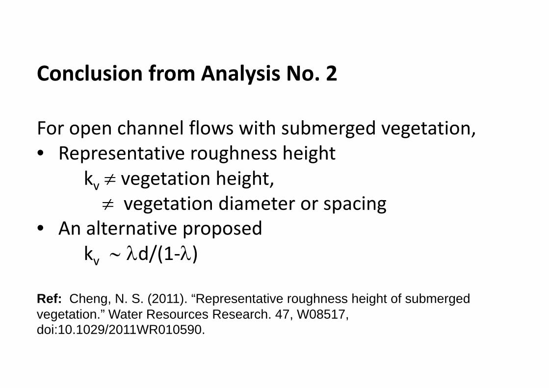
Conclusion from Analysis No. 2

For open channel flows with submerged vegetation,• Representative roughness height• Representative roughness height

kv ≠ vegetation height, ≠ vegetation diameter or spacing

• An alternative proposedp pkv ∼ λd/(1‐λ)

Ref: Cheng, N. S. (2011). “Representative roughness height of submerged vegetation.” Water Resources Research. 47, W08517, d i 10 1029/2011WR010590doi:10.1029/2011WR010590.

Topic No. 3

Scaling of velocity profiles for depth‐limited open channel flowsdepth limited open channel flows over simulated vegetation

43

Restrictions imposed

• Flow depth above vegetation is smallFlow depth above vegetation is small,  comparable to vegetation height

• Vegetation stems are rigid

1Power law (with exponent = 1/2.5 to 1/9)

0 8

= 0.0043 0.017 0.019 0.030s

yh

λ

0.8 0.030 0.077 0.119 m = 9

m = 2 5

s

0.6 m = 2.5

0.4

0.2

0 0.2 0.4 0.6 0.8 1 1.20

max

uu

45

max

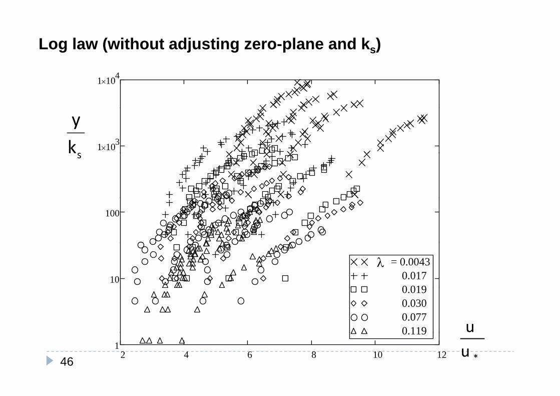
Log law (without adjusting zero-plane and ks)

1 104×

1 103×

s

yksk

100

10

= 0.0043 0.017

0 019

λ

0.019 0.030 0.077

0 119 u

46 2 4 6 8 10 121

0.119

*u

Velocity-defect law1

= 0.0043 0.017y λ

0.8

0.019 0.030 0.077 0.119

sh

0.6

0.4

0.2

0maxu u−

47

1− 0 1 2 3 40

*u

Scaling proposed in present study

1.2 = 3 cm

5u Uhs

1

5 cm 7 cm 10 cm Eq. (9)

v

max v

u Uu U

−−

0.8

0.6

0 2

0.4

0 0 4 0 8 1 2 1 6 20

0.2

zz

48

0 0.4 0.8 1.2 1.6 21/2z

Open channel flow layout( f )• Outer region (log layer, surface layer)

• Inner region (viscous sublayer, buffer layer, log layer)

Roughness sublayer

50

Roughness sublayer ‐ Poorly understood

51

A source of Large‐scale turbulence

Finnigan Shaw & Patton 2009Finnigan, Shaw & Patton 2009

52

Vegetated channel flowsVelocity profile is always inflectional implying inherentVelocity profile is always inflectional, implying inherent instability. Raupach (1995) proposed mixing layer analogyfor atmospheric canopy flowsfor atmospheric canopy flows 

Experimental evidence

Case B30       λ = 7 69%; H = 20 cm; Q = 9 6 L/s; S = 0 004;λ = 7.69%; H = 20 cm; Q = 9.6 L/s; S = 0.004; Dye injected at η = 1 cm

Video clip

Case A30       λ = 1.73%; H = 17 cm; Q = 11 L/s; S = 0.004; 

i j dDye injected at η = ‐1 cm

Vegetated boundary differs from regularVegetated boundary differs from regular rough boundary

Near the boundary, turbulence production > dissipation, and inertial sublayer almost disappearsy pp

Turbulence is far from random andTurbulence is far from random, and dominated by coherent structure,

i th i i las in the mixing layer

56

For vegetated flows with limited depth,l b d::  Log‐layer may be squeezed out

::  Roughness sublayer may be dominant 

RSLz

log law

RSLhs

y log law

log law Observed  profile 

y

RSLhv

Relevant studies – inconclusive 

Atmospheric boundary layer Both roughness sublayer and log layer exist;Still apply log law to roughness layer, but with corrections (Raupach 1995)corrections (Raupach 1995)

Flows over gravel bedsgFlow velocity in interfacial sublayer (lower roughness sublayer) may be linear.(Nikura JHE 2007; 2001)

A new trial :‐

Scaling variables

Length scale: half‐thickness (as used for jets)Velocity scale: maximum velocity difference at free surface

oumax‐uv

( )/

z1/2

oNormalized variables

z

(umax‐uv)/2(u‐uv)/(umax –uv)

zz/z1/2

Scaling proposed in present study

1.2 = 3 cm

5u Uhs

1

5 cm 7 cm 10 cm Eq. (9)

v

max v

u Uu U

−−

0.8

0.6

0 2

0.4

0 0 4 0 8 1 2 1 6 20

0.2

zz

60

0 0.4 0.8 1.2 1.6 21/2z

Explanation with a viscosity model

C l l i h i id h di lControl volume with unity width perpendicular to flow direction

o Δx

P1

x

z τΔx

P2 x

z

W

τΔx

W

61

du gzSd

= − Assume that ε(u - Uv) is weakly z-dependent in a power-law form i edz ε dependent in a power-law form, i.e. ε(u - Uv) ∼ zn

u+ = (u - Uv)/( gz1/2S)1/2, z+ = z/z1/2

( )1u Bexp z

β+ +⎡ ⎤= −⎢ ⎥αβ⎣ ⎦

vu U zexp ln(2)

u U z

β⎡ ⎤⎛ ⎞− ⎢ ⎥= − ⎜ ⎟⎜ ⎟⎢ ⎥⎝ ⎠αβ⎣ ⎦ max v 1/2u U z⎜ ⎟− ⎢ ⎥⎝ ⎠⎣ ⎦

62

Evaluation of β and z1/2

1.6

1.4

1.5This studyLiu et al. (2008)Yang & Choi (2009) Eq. (10)

1/2

s

z

h

1.2

1.3

q ( )

4 4⎡ ⎤⎛ ⎞

β ≈ 1.66

0 9

1

1.1 4.4

1/2 s v s v

s max v max v

z U U U U0.89 exp

h u U u U

⎡ ⎤⎛ ⎞− −⎢ ⎥= ⎜ ⎟− −⎢ ⎥⎝ ⎠⎣ ⎦

0.7

0.8

0.9⎣ ⎦

0.6 0.65 0.7 0.75 0.8 0.85 0.90.5

0.6

U U−

  

s v

max v

U Uu U

−−

63

Collapsing of the 24 velocity profiles measured for 4 difference flo depths and 6 different e etation on entrations 

1.2

flow depths and 6 different vegetation concentrations

1

= 3 cm 5 cm 7 cm 10 cm

v

max v

u Uu U

−−

hs

0.8

Eq. (9)

vu U−

0.6max vu U−

0.4

0.2 z

0 0.4 0.8 1.2 1.6 20

1/2

zz

1/2z64

Comparison with previously measured 26 velocity profiles

1.2Li t l (2008) T t 31

profiles

1

Liu et al. (2008), Test 31Liu et al. (2008), Test 32Liu et al. (2008), Test 33Liu et al. (2008), Test 34 Yang & Choi (2009) Test RH2Q1u U−

0.8

Yang & Choi (2009), Test RH2Q1 Yang & Choi (2009), Test RH2Q2 Eq. (9)

v

max v

u Uu U−

vu U−0.6max vu U−

0.4

0

0.2

z0 0.4 0.8 1.2 1.6 2

1/2

zz 1/2z

65

Conclusion from Analysis No. 3

• Flow depth is not a good length scale • Half‐thickness performs better in collapsing vel profiles; it measures the size of large scalevel profiles; it measures the size of large‐scale turbulence

Ref: Cheng, N. S., Nguyen, H. T., Tan, S. K., and Shao, S. (2012). “Scaling of velocity profiles for depth-limited open channel flows over submerged rigid vegetation.” Journal of Hydraulic Engineering, ASCE.

66

y g g,

Implication for other flows subject to large‐scale roughness

67

Implication for other flows subject to large‐scale roughness

R h bl d i d b fRoughness sublayer dominated by forest canopy

68

Future works

• Sediment transport in the presence of vegetation

• Effect of bedforms on characteristics of vegetated open channel flows

69

70