Variance estimation and weighting in...

quad

5. Model versus design6. Weighting in regression – a different view7. Boostrap reconsidered and use of replicate weights8. And finally ...

Variance estimation and weighting in regressionJean Monet Lecture in Pisa – 2018

Ralf MunnichTrier University, Faculty IV

Chair of Economic and Social Statistics

Pisa, 08st May 2018

Pisa, 08st May 2018 | Ralf Munnich | 1 (50) Weighting Methods in Regression


5. Model versus design

6. Weighting in regression – a different view

7. Boostrap reconsidered and use of replicate weights

8. And finally ...



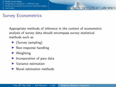
Survey Econometrics

Appropriate methods of inference in the context of econometricanalysis of survey data should encompass survey statisticalmethods such as

I (Survey sampling)

I Non-response handling

I Weighting

I Incorporation of para data

I Variance estimation

I Novel estimation methods



Design-based vs. model-based inference

I The use of survey weights is common practice in thetraditional survey statistics context, e.g. in the descriptiveanalysis of survey data.

I In contrast, the pros and cons of using survey weights whenanalysing data using statistical models are still discussed inthe literature.

I Design-based vs. model-based approach



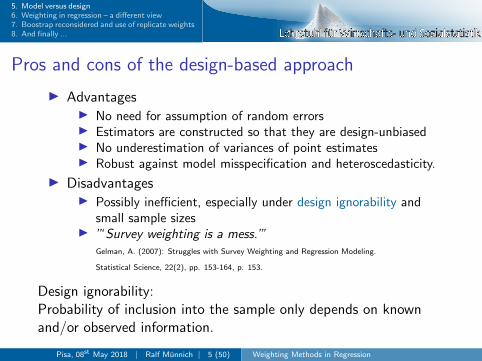
Pros and cons of the design-based approach

I AdvantagesI No need for assumption of random errorsI Estimators are constructed so that they are design-unbiasedI No underestimation of variances of point estimatesI Robust against model misspecification and heteroscedasticity.

I DisadvantagesI Possibly inefficient, especially under design ignorability and

small sample sizesI ”‘ Survey weighting is a mess.”’

Gelman, A. (2007): Struggles with Survey Weighting and Regression Modeling.

Statistical Science, 22(2), pp. 153-164, p. 153.

Design ignorability:Probability of inclusion into the sample only depends on knownand/or observed information.



Pros and cons of the model-based approach

I AdvantagesI If model is correctly specified, the unweighted estimators are

efficient

I DisadvantagesI Assumptions about errors are restrictiveI Model misspecification may lead to bias and even to design-

inconsistent estimatorsI ”‘ Essentially, all models are wrong, some are useful.”’

Box, G.E.P. a. N.R. Draper (1987): Empirical Model-Building and Response Surfaces. p. 424.



Example 1 - SHIW 2006

Faiella, I. (2010): The Use of Survey Weights in Regression Analysis. Banca d’Italia Working Papers - 739.



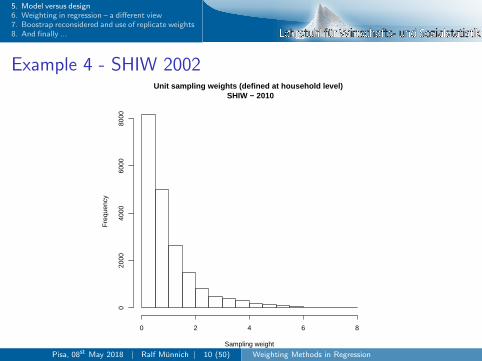
Example 4 - SHIW 2002Unit sampling weights (defined at household level)

SHIW − 2010

Sampling weight

Fre

quen

cy

0 2 4 6 8

020

0040

0060

0080

00

Faiella, I. (2008): Accounting for Sampling Design in the SHIW. Banca d’Italia Working Papers - 662.



Reasons for weightingI Purpose: Estimate population descriptive statistics.

Correct for:I Sampling Design (e.g. oversampling)I Non-responseI Frame errorsI Fitting to known marginal distributions

(e.g. calibration or post stratification)I Purpose: Estimate conditional expectations, maybe causal

effects.I correct for heteroskedasticityI correct for endogenous sampling / informative designI identify average partial effects in the presence of unmodeled

heterogeneity of effects

Reasons for and the choice of weighting methods are not clearlyseperable. Many problems have multiple possible occurences. E.g.sampling design and informative samples



Oversampling

Analogous to πps sampling, where a certain variable y is of centralimportance, in many cases certain subpopulations play a major rolein the estimation of the population parameters of interest.

In this case a disproportionately high inclusion probability may beassigned to units within relevant subpopulations. This approach iscalled oversampling.

Oversampling, if applied correctly, may lead to more preciseestimates or lower costs (through reduced sample sizes). Thecorrection of non-response bias might be facilitated as well.

As a prerequisite, auxiliary information is needed to identify therelevant subpopulation. Ideally, as in πps sampling, the auxiliaryinformation and the variables of interest are highly correlated.



Oversampling in wealth surveysI Wealth distribution highly skewed

I Gini coefficient of household wealth in Italy (2010): 0.624I Gini coefficient of household income in Italy (2010): 0.351I Banca d’Italia (2012):

Household Income and Wealth in 2010. Supplements to the Statistical Bulletin – Sample Surveys 6.

I Very few households hold majority of wealthI Concentration may well keep on rising

(see discussions about Thomas Piketty’s book)I Wealth surveys aim at precise estimation of the wealth

distributionI Wealth surveys cover asset holdings as wellI Estimation of financial asset holdings needs good coverage of

right tail of wealth distributionI Non-response typically much higher in wealth surveys

(sensitivity of subject and complex questions)I Wealth surveys like the Survey of Consumer Finances (SCF)

and the Eurosystem Household Finance and ConsumptionSurvey (HFCS) strive to apply effective oversampling routines



0.0 0.2 0.4 0.6 0.8 1.0

0.0

0.2

0.4

0.6

0.8

1.0

Net wealth and gross income Lorenz curves of households in DE

% of households

% o

f tot

al n

et w

ealth

/gro

ss in

com

e

Net wealthGross income

Data source: Eurosystem Household Finance and Consumption Survey (2013).



0.0 0.2 0.4 0.6 0.8 1.0

0.0

0.2

0.4

0.6

0.8

1.0

Net wealth and gross income Lorenz curves of households in BE

% of households

% o

f tot

al n

et w

ealth

/gro

ss in

com

e

Net wealthGross income




lowest 50% 50%−90% 90%−95% 95%−99% highest 1%

Share of total net worth held by group

Net worth group

%

010

2030

40

without oversamplingwith oversampling

lowest 50% 50%−90% 90%−95% 95%−99% highest 1%

Standard error of estimate

Net worth group

Sta

ndar

d er

ror

01

23

45

6


lowest 50% 50%−90% 90%−95% 95%−99% highest 1%

Number of observations

Net worth group

Obs

erva

tions

050

015

0025

00


Data source: Kennickell, A.B. (2007): The Role of Over-sampling of the Wealthy in the Survey of ConsumerFinances.



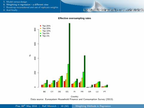
Oversampling in the HFCS

I Oversampling of wealthy households is implemented in 9 outof 15 HFCS country surveys(BE, CY, DE, ES, FI, FR, GR, LU and PT)

I Different auxiliary information used for routine(partially depending on institutional setting)I Electricity bill: CYI Geographical area: BE, DE, GR, PTI Income: FI, LUI Wealth: ES, FR

I Oversampling seems to have worked quite well in first wave ofHFCS

I Partially very complicated designs

I High variation of final household weights

I How to deal with such designs when analysing survey data?



BE CY DE ES FI FR GR LU PT

Effective oversampling rates

Country

%

020

040

060

080

0

Top 25%Top 20%Top 10%Top 5%Top 1%




Survey Weighted Regression I

In contrast to weighting for heteroscedasticity, weighting for surveyissues has the aim to expand the sample to a finite population.

That is, the units in the data set are weighted according to theirrelative importance for the estimation of the populationparameters.

Major reasons for the variation of weights in a data set:

I Sampling Design

I Non-response

I calibration to known marginals



Survey Weighted Regression II

The estimation can be performed according to the WLS estimatorunder heteroscedasticity. E.g.,

I compensating for different inclusion probabilities πi can be

done by using wi =1

πi.

I compensating for non-response via the modeling of responsepropensities which can be used to construct weights.

I accounting for known marginals via post-stratification weights.



Survey Weighted Regression IIIAs we know from generalized least squares the coefficients b maybe estimated via:

bw = (X ′WX )−1X ′Wy

In contrast to the case of generalize least squares for knowncovariance matrix, the σ2 has to be estimated, as variances are notknown.An approximately unbiased estimator for σ2

w is :

σ2w =

n∑i=1

wie2i

n∑j=1

wj − K − 1



Survey Weighted Regression IVAnd the variance of the b can be estimated design consistent undera single-stage, unstratified and unclustered design where units areselected with probabilities πi = 1/wi with replacement.

V(bw ) = (X ′WX )−1(n∑

i=1

x ′i wie2i wixi )(X ′WX )−1

As can rapidly be seen, under more complex designs, the formulasfor the variance estimation get much more complicated.

Under complex survey designs, often the easiest solution is to useresampling techniques.

Li, Jianzhu, and Richard Valliant. “Influence analysis in linear regression with

sampling weights.“ 2006. Proceedings of the Section on Survey Research

Methods (2006).



Residual bootstrapConsider the linear regression

yi = yi + εi ,

then instead of resampling the observations the residuals may beresampled.

1. Fit the linear regression model, and store y and e.

2. Generate y∗(r)i = yi + ei , where ej is drawn with replacement

from e.3. Fit the linear regression model as before, just replace y with

y∗(r)i . Extract the information of interest h∗(r) from the

regression model (usually the coefficients).4. Repeat steps 2 and 3 R times and compute afterwards the

bootstrap estimates.

Usually the choice of the residual type has no large impact on theresults. If in doubt use studentized residuals.



Wild Bootstrap I

The Wild Bootstrap is constructed to be used underheteroskedasticity.

1. Fit the linear regression model, and store y and e.

2. Generate y∗(r)i = yi + ν

∗(r)i ei , where ν

∗(r)i is a realization of a

random variable.

3. Fit the linear regression model as before, just replace y with

y∗(r)i . Extract the information of interest h∗(r) from the

regression model (usually the coefficients).

4. Repeat steps 2 and 3 R times and compute afterwards thebootstrap estimates.



Wild Bootstrap II

Popular choices of νi are

I standard normal distribution

I Radermacher distribution

νi =

{−1 probability of 0.5

1 probability of 0.5

I Mammen’s two-point distribution

νi =

−√

5− 1

2probability of

√5 + 1

2√

5√5 + 1

2probability of

√5− 1

2√

5



Wild Bootstrap III

I Radermacher Distribution seems to outperform in many casesMammen’s two-point distribution.

I Radermacher Distribution assumes symmetries, butMammen’s two-point distribution gets the fourth momentwrong.

I In the linear regression, depending on the choice of ν the WildBootstrap for variance estimation of the regression parametersconverge to robust standard errors.



Parametric bootstrap

In the case of parametric bootstrap the empirical distributionfunction is replaced by an estimated parametric distribution.Especially in small sample cases this might give better results.



Considering the Design

I When making bootstraps the design of the sample has to beconsidered.

I That means, if nh elements were drawn from the h-thstratum, then it should follow n∗h = nh

I If the observed units were drawn in clusters, e.g. severalpersons per household, where the household are the samplingunits, then the sampling units have to resampled.

I This has also to be considered in multi-stage designs.

I However, in many applications the information on clusters andstrata may be retained due to disclosure risks.

I Is there a way to do the right bootstrap, without having thefull design information?



Replicate Weights

If the data producer can not give the necessary information inorder to allow for correct resampling, he can provide a set ofreplicate weights.

I Use the appropriate resampling techniques, obtaining Rresamples s∗(r), r = 1 . . .R.

I Recalculate the weights w∗(r), in the same manner it wasdone for the full sample s∗(r).

I Use the sample s∗(r) with the weights w∗(r) to compute theestimate of interest h∗(r).

I Take the resampling distribution of h∗(r) for the computationof variances.



Design information in scientific use files

I Data producers do not always provide survey designinformation(like e.g. stratum identifiers) with scientific use files of microdata

I Some reasons for withholding such information:I Concerns about confidentiality

(e.g. re-identification risk when first level of stratification isgeographic)

I Majority of data users may (unfortunately) not care aboutsurvey design

I Correct variance estimation for complex survey designs may betoo difficult for typical data users



Provision of replicate weights

I Resampling techniques, like the different variants ofbootstrapping, are quite flexible and do not require explicitformulas

I Without full design information data users cannot usebootstrapping per se

I Solution is a simulation of bootstrapping using sets ofso-called replicate weights mimicking the repeated drawing ofsub samples(see above)

I Typically a large number of such replicate weights is providedin scientific use files



Replicate weighting in the HFCS

I The Eurosystem Household Finance and ConsumptionNetwork (HFCN) used the rescaling bootstrap of Rao and Wu(1988) and Rao et al. (1992) in the context of the HFCS

I For each unit (household) the HFCN provides a set of 1,000replicate weights in the micro data set

I Replicate weights were generated using SAS and Stataroutines

I Additional calibration step (equal to treatment of finalweights)



Variance estimation in the HFCSThe multiple stochastic imputation routine used in dealing withitem non-response in core survey items (relating to wealth etc.)has to be taken into account as well.

Exemplary variance estimation for the total of y (θ) usingI n final household weights (wi , i = 1, . . . , n),I n · R replicate weights (ωir , i = 1, . . . , n, r = 1, . . . ,R) andI M imputed data sets (m = 1, . . . ,M)

following Rubin (1987) and HFCN (2013):

θm =n∑

i=1

wi · yim ∀ m (m = 1, . . . ,M)

θmr =n∑

i=1

ωir · yim ∀ m (m = 1, . . . ,M), r (r = 1, . . . ,R)



Variance estimation in the HFCS (2)

θm =1

R·

R∑r=1

θmr ∀ m (m = 1, . . . ,M)

Um =1

R − 1·

R∑r=1

(θmr − θm)2 ∀ m (m = 1, . . . ,M)

W =1

M·

M∑m=1

Um

θ =1

M·

M∑m=1

θm



Variance estimation in the HFCS (3)

Q =1

M − 1·

M∑m=1

(θm − θ

)2

Finally, using the within-imputation variance (W ) and thebetween-imputation variance (Q), the total variance (T ) may becalculated as:

T = W +(1 + M−1

)· Q

A combination of the R packages survey and mitools (cf.Lumley, 2010 and 2014) can deal with such a setup, but is quitecumbersome to use. Custom-made functions can be faster.



Unavoidable trade-off and user discretion

I Small number of replications ⇒ (potentially) no convergence

I Large number of replications ⇒ long computation time

I Data user faces inherent trade-off

I Data user has discretion over choice of number of replicateweights to be used

I Data user has leeway for manipulative use of replicate weights

I Finding appropriate critical values for significance tests in sucha setting is a non-trivial task, allowing additional userdiscretion.

Discuss:What should a data user do in case of seemingly randomly missingreplicate weights throughout a whole country data set?



Illustrating the problemsThe associated problems can be illustrated by estimating a logitmodel to explain a household’s probability to hold at least onemortgage using HFCS data (cf. Bover et al., 2014). Theexogenous variables used cover socio-demographic characteristicsof the household’s core members as well as the number of adultmembers and the household’s total gross income.The model is estimated for 11 countries in the following variants:

1. Naive: No weights used2. Weighted: Final weights used3. Design-based 100: First 100 replicate weights used4. Significant: 100 replicate weights resulting in lowest estimated

variance used5. Non-significant: 100 replicate weights resulting in highest

estimated variance used6. Design-based 1,000: All 1,000 replicate weights usedPisa, 08st May 2018 | Ralf Munnich | 37 (50) Weighting Methods in Regression


Naive

Estimate Std. error z Signif.

(Intercept) -6.2787 1.447906 -4.336 ***

age_16_34 -0.4983 0.230202 -2.165 **

age_45_54 -0.6053 0.224987 -2.691 ***

age_55_64 -0.5830 0.245051 -2.379 **

age_above_65 -1.4861 0.385968 -3.850 ***

age_diff 0.0379 0.024843 1.525

edu_low -0.0685 0.218294 -0.314

edu_high 0.1008 0.185546 0.543

edu_diff 0.1176 0.191418 0.614

emp_self -0.0915 0.237936 -0.384

emp_ret -1.0581 0.323465 -3.271 ***

emp_inact_un -0.7540 0.392399 -1.921 *

partner_emp 0.3620 0.200540 1.805 *

log_adult 0.1768 0.207858 0.851

log_inc 0.5575 0.133216 4.185 ***



Weighted


(Intercept) -7.7075 1.530110 -5.037 ***

age_16_34 -0.3223 0.217942 -1.479

age_45_54 -0.6323 0.226648 -2.790 ***

age_55_64 -0.4067 0.264630 -1.537

age_above_65 -1.5237 0.447095 -3.408 ***

age_diff 0.0475 0.027408 1.734 *

edu_low -0.1230 0.198272 -0.620

edu_high 0.0107 0.195933 0.054

edu_diff 0.1565 0.201387 0.777

emp_self -0.1688 0.312497 -0.540

emp_ret -0.9612 0.370500 -2.594 ***

emp_inact_un -0.8635 0.391238 -2.207 **

partner_emp 0.4560 0.207779 2.195 **

log_adult 0.1027 0.212504 0.483

log_inc 0.6802 0.142425 4.776 ***



Design-based 100


(Intercept) -7.7075 1.873515 -4.114 ***

age_16_34 -0.3223 0.241787 -1.333

age_45_54 -0.6323 0.254407 -2.485 **

age_55_64 -0.4067 0.285327 -1.425

age_above_65 -1.5237 0.492477 -3.094 ***

age_diff 0.0475 0.027592 1.722 *

edu_low -0.1230 0.244550 -0.503

edu_high 0.0107 0.212018 0.050

edu_diff 0.1565 0.233819 0.669

emp_self -0.1688 0.338755 -0.498

emp_ret -0.9612 0.421281 -2.282 **

emp_inact_un -0.8635 0.468787 -1.842 *

partner_emp 0.4560 0.238829 1.909 *

log_adult 0.1027 0.245242 0.419

log_inc 0.6802 0.178875 3.803 ***



Significant


(Intercept) -7.7075 0.802204 -9.608 ***

age_16_34 -0.3223 0.212764 -1.515

age_45_54 -0.6323 0.207368 -3.049 ***

age_55_64 -0.4067 0.239040 -1.701 *

age_above_65 -1.5237 0.280574 -5.431 ***

age_diff 0.0475 0.030142 1.576

edu_low -0.1230 0.195971 -0.628

edu_high 0.0107 0.182384 0.059

edu_diff 0.1565 0.187934 0.832

emp_self -0.1688 0.261167 -0.646

emp_ret -0.9612 0.271325 -3.543 ***

emp_inact_un -0.8635 0.329870 -2.618 ***

partner_emp 0.4560 0.187901 2.427 **

log_adult 0.1027 0.217782 0.472

log_inc 0.6802 0.076118 8.936 ***



Non-significant


(Intercept) -7.7075 3.863880 -1.995 **

age_16_34 -0.3223 0.264625 -1.218

age_45_54 -0.6323 0.254261 -2.487 **

age_55_64 -0.4067 0.343336 -1.185

age_above_65 -1.5237 0.543656 -2.803 ***

age_diff 0.0475 0.028588 1.662 *

edu_low -0.1230 0.308104 -0.399

edu_high 0.0107 0.257177 0.042

edu_diff 0.1565 0.294790 0.531

emp_self -0.1688 0.349501 -0.483

emp_ret -0.9612 0.453414 -2.120 **

emp_inact_un -0.8635 0.606371 -1.424

partner_emp 0.4560 0.202479 2.252 **

log_adult 0.1027 0.295666 0.347

log_inc 0.6802 0.356598 1.907 *



Design-based 1,000


(Intercept) -7.7075 1.947833 -3.957 ***

age_16_34 -0.3223 0.262167 -1.229

age_45_54 -0.6323 0.258428 -2.447 **

age_55_64 -0.4067 0.311386 -1.306

age_above_65 -1.5237 0.511940 -2.976 ***

age_diff 0.0475 0.029689 1.600

edu_low -0.1230 0.238568 -0.516

edu_high 0.0107 0.232261 0.046

edu_diff 0.1565 0.246025 0.636

emp_self -0.1688 0.322827 -0.523

emp_ret -0.9612 0.425495 -2.259 **

emp_inact_un -0.8635 0.503979 -1.713 *

partner_emp 0.4560 0.229529 1.987 **

log_adult 0.1027 0.255610 0.402

log_inc 0.6802 0.180461 3.769 ***



z values of mortgage model parameter for LU|z| des geschätzten Regressionskoeffizienten der Variable age_diff

Anzahl verwendeter Replikationsgewichte

z(H

0:β

k=

0)

1.0

1.5

2.0

2.5

3.0

2 50 100 250 500 750 1000

krit. z (1%)krit. z (5%)krit. z (10%)




z values of mortgage model parameter for NL|z| des geschätzten Regressionskoeffizienten der Variable edu_diff


z(H

0:β

k=

0)

1.0

1.5

2.0

2.5

3.0

2 50 100 250 500 750 1000





z values of mortgage model parameter for FI|z| des geschätzten Regressionskoeffizienten der Variable partner_emp


z(H

0:β

k=

0)

1.0

1.5

2.0

2.5

3.0

2 50 100 250 500 750 1000





Preliminary conclusions

I Variance estimation using replicate weights not stable andprone to manipulation

I (Typical) ignorance of (replicate) weights seems negligent

I In the case of the HFCS data:Ideally use 1,000 replication weights, at least 350 replicationweights

I Data producers should consider provision of design information(possibly finding other ways to deal with re-identification risk)



How large is the sample space?

I Design optimization may lead to very small sample spaces, i.e.the number of all possible samples is very low

I In practice, this may be rejected as sampling procedure due tomissing randomness

I How large should a sample space be? How to we measure thisspace?

I Example: balanced sampling with (too) many constraints

I Possible solution: relaxing the hard constraints

I But this may lead to biased estimators!



Some more issues ...

Does modeling spoil the design world?

I Sample selection biases may occurI Example: oversampling high incomes (HFCS) in linear

regression may lead to biases of even wrong methodsI Can we easily use non-informative sampling methods?

How may synthetic data generation be influenced?

I Constructing synthetic household data relies onappropriate household and address structures. However,many marginal distributions are known on individual level.

I How can we (re-)sample from these distributions whileconsidering household interactions under marginalconstraints?

I Rejective sampling with changing probabilities may beone solution. How should we measure the outcome?



Can we think about BIG DATA subsampling?

Big data analytics always suffers from modeling on huge andunbalanced datasets!

I Interesting models do not work on that data unless newalgorithms are developed

I The data streams, are in general not balanced, i.e. biasedresults are very likely

I Sampling from big data may help to reduce the computationburden considerably while reducing the selection bias

I Sampling using satellite data is already known but does notconsider all peculiarities of interest

But this makes new sampling ideas necessary!


Variance estimation and weighting in...

Documents

Transcript of Variance estimation and weighting in...