VARDHMAN MAHAVEER OPEN UNIVERSITYassets.vmou.ac.in/MSCCH03.pdf · 2014-11-01 · decreases. (iii)...

MSCCH-03 VARDHMAN MAHAVEER OPEN UNIVERSITY

PHYSICAL CHEMISTRY

Course Development Committee Chair Person Prof. Vinay Kumar Pathak Vice-Chancellor Vardhaman Mahaveer Open University, Kota

Coordinator and Members Coordinator Dr. Arvind Pareek Director (Regional Centre) Vardhaman Mahaveer Open University, Kota Members: . Dr. Anuradha Dubey Deputy Director School of Science & Technology Vardhaman Mahaveer Open University, Kota

Dr. Sunil Kumar Jangir Asstt. Prof. Chemistry School of Science & Technology Vardhaman Mahaveer Open University, Kota

Dr. P.S. Verma (Retd.), Prof. of Chemistry University of Rajasthan

Dr. Pahup Singh (Retd.), Prof. of Chemistry University of Rajasthan

Dr. P.D. Sharma (Retd.), Prof. of Chemistry University of Rajasthan

Prof. Ashu Rani Prof. of Chemistry University of Kota, Kota

Dr. R.L. Pilaliya (Retd.), lecturer in Chemistry Govt. College, Bikaner

Dr. Sapna Sharma Prof. of Chemistry JECRC,university Jaipur

Dr. Sanjay Kumar Sharma Prof. of Chemistry JECRC,university Jaipur

Ms. Renu Hada Guest Faculty Chemistry Vardhaman Mahaveer Open University, Kota

Editing and Course Writing Editor Prof. Sapana Sharma JECRC University, Jaipur Course Writing Name of Writters Unit No. Dr. Deepti Goyal Assistant professor Gautam Buddha, University

8,9,17

Dr. Renuka Goyal Lecturer, Govt., College, Kota

1

Dr. Sapna Sharma Professor, JECRC, Jaipur

10,13,14,15

Dr. Vishwajeet Singh Yadav Assistant professor, Kadi Sarva University, Gandhi Nagar, Gujrat

3,4,11,12,21

Ekta Sakle Lecturer, Royal College, Ratlam

16,18,19,20

Dr. Romila Karnawat 5,6,7

Academic and Administrative Management

ISBN : All Right reserved. No part of this Book may be reproduced in any form by mimeograph or any other means without permission in writing from V.M. Open University, Kota. Printed and Published on behalf of the Registrar, V.M. Open University, Kota. Printed by :

Prof. Vinay Kumar Pathak Vice-Chancellor Vardhaman Mahaveer Open University, Kota

Prof. L.R.Gurjar Director (Academic) Vardhaman Mahaveer Open University, Kota

Prof. Karan Singh Director (MP&D) Vardhaman Mahaveer Open University, Kota

Dr. Anil Kumar Jain Additional Director (MP&D) Vardhaman Mahaveer Open University, Kota

MSCCH-03 PHYSICAL CHEMISTRY

Name of Unit

Unit - 1: State Functions and Differentials

Unit - 2 : Thermochemistry

Unit-3 : The Third Law of Thermodynamics

Unit - 4 : Combining First and Second Law

Unit - 5 : Phase Equilibria

Unit – 6 : Physical Transformation of Simple Mixtures

Uni - 7 : Quantum Chemistry

Unit – 8 : Simple Reaction

Unit – 9 : Enzyme Catalysis

Unit - 10 Fast Reactions

Unit-11 : Collision Theory

Unit-12 : Theories of Unimolecular Reactions

Unit- 13 : Statistical Thermodynamics

Unit - 14 : Partition Function

Unit - 15 : Statistics

Unit-16 : Non-equilibrium thermodynamics and Significance

Unit – 17 : UV-visible spectroscopy

Unit – 18 : Infrared spectroscopy

Unit – 19 : Raman spectroscopy

Unit -20 : Electronic spectroscopy of molecules

Unit-21 : NMR Spectroscopy

Page no

1-24

25-43

44- 65

66-83

84-108

109-130

131-165

167-207

208-234

234-245

246-263

264-283

284-295

296-307

308-320

321-336

336-371

372-389

390-407

408-429

430- 462

1

Unit - 1: State Functions and Differentials Structure of Unit:

1.0 Objectives

1.1 Introduction

1.2 Limitations of Thermodynamic system and process

1.3 Types of Thermodynamics

1.4 State Functions and Differentials

1.5 Internal Energy, E

1.6 First Law of Thermodynamics

1.7 Temperature Dependence of Heat

1.8 Adiabatic Expansion of an Ideal Gas

1.9 Reversible process

1.10 Irreversible process

1.11 Summary

1.12 Glossary

Answer to key assessment questions

1.13 Reference and Suggested readings

1.13 Review Question

At the end of the unit learner will be able:

To know about the various state functions and exact and inexact differentials.

To determine the internal energy and its temperature dependence.

To determine temperature dependence of enthalpy.

To deduce the work of reversible and irreversible adiabatic expansion.

1.0 Objectives

2

1.1 Introduction

The thermodynamic deals with the behavior of matter and the transformation between different forms of energy. The term 'Thermo' means heat and 'dynamics' means motion. Therefore, thermodynamics is concerned with the heat motion. It deals basically with heat and work in all types of physical and chemical process.

Thermodynamics is based on three generalizations, known as First, Second and Third law of thermodynamics. Since thermodynamics laws deal with energy, they are applicable to all the phenomena of nature. There is no formal proof for these laws. They are only based on human experiences. However nothing contrary to these laws has been known to happen in case of macroscopic systems, i.e., systems comparatively large and involving many molecules, ions, etc.

It is important to note that the laws of thermodynamics are not concerned at all with the atomic or molecular structure of matter.

1.2Limitations of Thermodynamics

Although the science of thermodynamics has wide applications, yet it has the following limitations.

i. The methods of thermodynamics are concerned with matter on the macroscopic scale, i.e., the system which are comparatively large and involve many molecules. It does not deal with microscopic objects such as individual atoms, molecules or ions.

ii. While it gives the relationship between various properties experimentally observed, it is unable to give the actual values of these properties and does not offer any explanation as to why these properties arise in a system.

iii. It fails to give any information regarding the time taken for the completion of a change and the rate at which a change takes place.

iv. It cannot explain completely the behavior of a system away from equilibrium. It deals with substances in stationary state or equilibrium state.

3

1.3 Types of Thermodynamics system and process

The important parts of the study of thermodynamics are a few terms and definitions, which must be understood clearly, and these are as follows:

1.3.1. System, boundary and surroundings: A thermodynamic system may be defined as any specified portion of matter in the universe which is under study. A system may consist of one or more substances.

The rest of the universe which might be in a position to exchange energy and matter with the system is called the surroundings.

Thus, the system is separated from the surroundings by a boundary which may be real or imaginary.

1.3.2. Homogeneous and Heterogeneous system: A system is said to be homogeneous when it is completely uniform throughout, for example, a pure solid or liquid or a solution or a mixture of gases. In other words, a homogeneous system consists of only one phase‘.

A system is said to be heterogeneous when it is not uniform throughout. In other words, a heterogeneous system is one which consists of two or more phases. Thus a system consisting of two or more immiscible liquids or a solid in contact with a liquid in which it does not dissolve, is a heterogeneous system. A liquid in contact with its vapour is also a heterogeneous system because it consists of two phases.

1.3. 3. Types of Thermodynamic Systems: There are three types of thermodynamic systems, depending on the nature of the boundary which are as follows:

(i) Isolated system: When the boundary is both sealed and insulated, no interaction is possible with the surroundings. Therefore,

An isolated system is one that can transfer neither matter nor energy to and from, its surroundings. .

(ii) Closed system: Here the boundary is sealed but not insulated. Therefore, A closed system is one which cannot transfer matter but can transfer energy in the form of heat, work and radiation to and from its surroundings.

(iii) Open system: In such system the boundary is open and un isolated therefore,

4

An open system is one which can transfer both energy and matter to and from its surroundings.

1.3.4. Macroscopic System: The word macroscopic means ‘on a large scale.’ This term, therefore, is used to convey the sense of appreciable quantities i.e. quantities which can be weighed.

A system is said to be macroscopic when it consists of a large number of molecules, atoms or ions.

1.3.5. Macroscopic Properties: The properties associated with a macroscopic system are called macroscopic properties.

These properties are pressure, volume, temperature, composition, density, viscosity, surface tension, refractive index, colour etc.

1.3.6. Extensive and Intensive Properties: All macroscopic or bulk properties of the system (volume, pressure, mass etc.), irrespective of whether they are state variables or not can be divided into two classes:

An extensive property of a system is that which depends upon the amount of the substance or substances present in the system. The examples are mass, volume, energy, heat capacity, enthalpy, entropy, free change etc.

An intensive property of a system is that which is independent of the amount of the

substance present in the syste1′n.The examples are temperature, pressure, density, viscosity, refractive index, surface tension and specific heat.

1.3.7. Thermodynamic Equilibrium: A system in which the macroscopic properties do not undergo any change with time is said to be in thermodynamic equilibrium.

Suppose a system is heterogeneous, if it is in equilibrium. The macroscopic properties in the various phases remain unchanged with time.

Actually, the term thermodynamic equilibrium implies the existence of three kinds of equilibria system. These are:

(i) Thermal equilibrium: A system is said to be in thermal equilibrium if there is no flow of heat from one position of the system to another. This is possible if the temperature remains the same throughout in all parts of the system.

5

(ii) Mechanical equilibrium: A system is said to be in mechanical equilibrium if no mechanical work is done by one part of the system on another part of the system. This is possible if the pressure remains the same throughout in all parts of the system.

(iii) Chemical equilibrium: A system is said to be in chemical equilibrium if the composition of the various phases in the system remains the same throughout.

1.3.7 Thermodyname. Process: Whenever the state of a system changes, it is said to have undergone a process. Thus a process may be defined as the operation by which a system changes from one state to another.

The following types of process are known:

(i) Isothermal process (T remains constant): It is the process in which the temperature of the system remains constant during each step. In such a process the systems are in thermal contact with a constant temperature and exchange heat with surroundings ( T = 0)

(ii) Adiabatic process (Thermally insulated from the surroundings): A process in which no heat is exchanged between the system and surroundings is called adiabatic process (Q=O). System in which such processes occur are thermally insulated from the surroundings. In such processes, the temperature of the system may change according to the conditions. For example, if heat is evolved in the system, the temperature of the system increases and if heat is absorbed, the temperature decreases.

(iii) Isochoric process (V remains constant): A process in which the volume of the system remains constant during each step of the change system is called isochoric process .

The reaction occurring in sealed containers of constant volume correspond to such processes.

(iv) Isobaric process (P remains constant): It is the process in which the pressure

of the system remains constant during each step of the system ).

When a reaction occurs in an open beaker which will be at one atmosphpric pressure, the process is called isobaric process.

(v) Cyclic process: The process which brings aback a system to its original state after a series of changes is called a cyclic process.

Here = 0 (Enthaply change),

6

(Internal energy change),

(Entropy change)

1.4 State Functions and Differentials

1.4.1 State of System and State Variables:

When macroscopic properties of a system have definite values, the system is said to be in a definite state. Whenever there is a change in any one of the macroscopic properties, the system is said to change into a different state. Thus the state of a system is fixed by its macroscopic properties.

Since the state of a system changes with the change in any of the macroscopic properties, these are called state variables. It also follows that when a system changes from one state (called initial state) to another state (called final state), there is invariably a change in one or more of the macroscopic properties.

Pressure, temperature, volume, mass and composition are the most important variables. In actual practice it is not necessary to specify all the variables because some of them are interdependent. In the case of a single gas, composition is not one of the variables because it remains always 100%.

Further, if the gas is ideal and one mole of the gas is under examination, it obeys the gas equation, PV = RT, where R is the universal gas constant. Evidently, if only two of the three variables (P, V and T) are known, the third can be easily calculated. Let the two variables be temperature and pressure. These are called independent variables. The third variable, generally volume, is said to be a dependent variable as its value depends upon the values of P and T. Thus, the thermodynamic state of a system consisting of a single gaseous substance may be completely defined by specifying any two of the three variable e.g. temperature, pressure and volume.in a closed system, consisting of one or more components mass is not a state variable.

1.4.2 Exact and inexact differentials

A thermodynamic property is a state function when a change in its value from an initial state (1) to a final state(2) does not depend on the path of the process. A differential of such a property is called Exact Differential. For example Pressure, Volume, Temperature and Energy are thermodynamic properties and hence called

7

state functions. An exact differential on integration yields a definite value. For example,

is just the difference between the mean energy of the system in the final macrostate and the initial macrostate, in the limit where these two states are nearly the same. It follows that if the system is taken from an initial macrostate to any final macrostate the mean energy change is given by

However, since the mean energy is just a function of the macrostate under consideration, and depend only on the initial and final states, respectively. Thus, the integral depends only on the initial and final states, and not on the particular process used to get between them.

Consider, now, the infinitesimal work done by the system in going from some initial macrostate to some neighbouring final macrostate. In general, work is not the difference between two numbers referring to the properties of two neighbouring macrostates. Instead, it is merely an infinitesimal quantity characteristic of the

process of going from initial state to final state. In other words, the work δw is in general an inexact differential. The total work done by the system in going from any macrostate initial to some other macrostate final cannot be written as the internal energy. So

Wif ≠

Small changes in the state functions or path in dependent functions are denoted by symbols like dE, dH, dS, dG etc. On the other hand, small changes in path dependent

functions like q and w are denoted by δq, δw etc.

1.4.3The Euler Reciprocal Relation

let F be a state function of two independent variables x and y of the system then

F=(x,y)

As F is a state function, it can be written as exact differentials

8

It can be written as

Where M(x,y)=

And N(x,y)=

In mathematical thermodynamics, the Eulerreciprocity relation or "reciprocity relation" for the above functions can be written as

1.5 Internal Energy, E

Every substances associated with a definite amount of energy which depends up on its chemical nature as well as up on its temperature, pressure and volume. This energy is known as internal energy. Absolute value of internal energy of a system cannot be determined because it is not possible to determine the exact values of constituent energies such as translational energy, nuclear energy and vibrational energy. Internal energy of a system is the inherent energy present in the system by virtue of its position. It is a state function. It is true that the actual value of internal energy cannot be determined but, fortunately, in thermodynamics the absolute value is not of any significance. It is the change in internal energy accompanying a chemical or physical process that is of interest and this is a measurable quantity.

The internal energy of a system is represented by the symbol E (Some books use the symbol U). It is neither possible nor necessary to calculate the absolute value of internal energy of a system. In thermodynamics we are concerned only with the

energy changes when a system changes from one state to another. If E be the difference of energy of the initial state (Ein) and the final state (Ef),

we can write

9

E = Ef – Ein

E is +ve if Ef is greater than Ein and –ve if Ef is less than Ein.

A system may transfer energy to or from the surroundings as heat or as work, or both.

Units of Internal Energy

The SI unit for internal energy of a systemis the joule (J). Another unit of energy which is not an SI unit is the calorie, 1 cal = 4.184 J.

1.6First Law of Thermodynamics

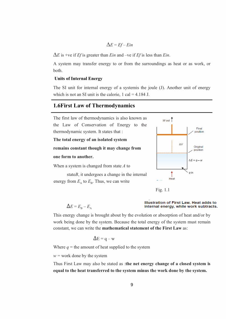
The first law of thermodynamics is also known as the Law of Conservation of Energy to the thermodynamic system. It states that :

The total energy of an isolated system

remains constant though it may change from

one form to another.

When a system is changed from state A to

stateB, it undergoes a change in the internal energy from EA to EB. Thus, we can write

Fig. 1.1

ΔE = EB – EA

This energy change is brought about by the evolution or absorption of heat and/or by work being done by the system. Because the total energy of the system must remain constant, we can write the mathematical statement of the First Law as:

ΔE = q – w

Where q = the amount of heat supplied to the system

w = work done by the system

Thus First Law may also be stated as :the net energy change of a closed system is equal to the heat transferred to the system minus the work done by the system.

10

1.7 Temperature Dependence of Heat

1.7.1 Molar Heat Capacities

Heat capacity of a system mean the capacity to absorb heat and store energy. As the system absorbs heat, it goes into the kinetic motion of the atoms and molecules contained in the system. This increased kinetic energy raises the temperature of the system.

If q calories is the heat absorbed by mass m and the temperature rises from T1 to T2, the heatcapacity (c) is given by the expression

Thus heat capacity of a system is the heat absorbed by unit mass in raising the temperature by one degree (K or º C) at a specified temperature.

When mass considered is 1 mole, the expression (1) can be written as

whereC is denoted as Molar heat capacity.

The molar heat capacity of a system is defined as the amount of heat required to raise the temperature of one mole of the substance (system) by 1 K.

Since the heat capacity (C) varies with temperature; its true value will be given as

wheredq is a small quantity of heat absorbed by the system, producing a small temperature rise dT.

Thus the molar heat capacity may be defined as the ratio of the amount of heat absorbed to the rise in temperature.

1.7.2 Units of Heat Capacity

The usual units of the molar heat capacity are calories per degree per mole (cal K–1 mol–1), or joules per degree per mole (J K–1 mol–1), the latter being the SI unit.

11

Heat is not a state function, neither is heat capacity. It is, therefore, necessary to specify the

process by which the temperature is raised by one degree. The two important types of molar heat capacities are those : (1) at constant volume; and (2) at constant pressure.

1.7.3 Molar Heat Capacity at Constant Volume

According to the first law of thermodynamics

....(3)

Dividing both sides by dT, we have

....(4)

At constant volume dV = 0, the equation reduces to

Thus the heat capacity at constant volume is defined as the rate of change of internal energy with temperature at constant volume.

1.7.4 Molar Heat Capacity at Constant Pressure

Equation (4) above may be written as

...(5)

We know H = E + PV

Differentiating this equation w.r.t T at constant pressure, we get

...(6)

12

comparing it with equation (5) we have

Thus heat capacity at constant pressure is defined as the rate of change of enthalpy with temperature at constant pressure.

1.7.5 Relation Between Cp and Cv

From the definitions, it is clear that two heat capacities are not equal and Cp is greater than Cv by a factor which is related to the work done. At a constant pressure part of heat absorbed by the system is used up in increasing the internal energy of the system and the other for doing work by the system. While at constant volume the whole of heat absorbed is utilized in increasing the temperature of the system as there is no work done by the system. Thus increase in temperature of the system would be lesser at constant pressure than at constant volume. Thus Cp is greater than Cv.

We know

...(7)

and

...(8)

By definition

H = E + PV (for 1 mole of an ideal gas)

or H = E + RT

( PV = RT)

Differentiating w.r.t. temperature, T, we get

[By using equation (7) and (8)]

13

Thus Cp is greater than Cvby a gas constant whose value is 1.987 cal K–1 mol–1 or 8.314 J K–1Md-1

S.I. units.

1.7.6 Calculation of E and H

(A) E : For one mole of an ideal gas, we have

Or

For a finite change, we have

and for n moles of an ideal gas we get

(B) H : Weknow

and for n moles of an ideal gas we get

14

SOLVED PROBLEM 1. Calculate the value of ΔE and ΔH on heating 64.0 g of oxygen from 0ºC to 100ºC. Cv and Cp on an average are 5.0 and 7.0 cal mol–1 degree–1.

SOLUTION.We know

1.2 State true or false in following statements

a) A differential of a property where its value does not depend on path of

process is exact differentials (T/F)

b) A definite amount of energy associate with the substance is activation

energy (T/F)

c) According to first low, total energy of isolated system change from one

form to another (T/F)

d) Heat capacity at constant volume is rate of change of internal energy with

temperature at constant volume. (T/F)

1.8Adiabatic Expansion of An Ideal Gas

A process carried in a vessel whose walls are perfectly insulated so that no heat can pass through them, is said to be adiabatic. In such a process there is no heat exchange between a system and surroundings, and q = 0.

15

According to the First law

E = q – w = 0 – w

Or E = – w ...(9)

Since the work is done at the expense of internal energy, the internal energy decreases and the temperature falls.

(a) Relation between Temperature and Volume

Consider 1 mole of an ideal gas at pressure P and a volume V. For an infinitesimal increase in volume dV at pressure P, the work done by the gas is –PdV. The internal energy decreases by dE.

According to equation (9)

dE= – PdV ...(10)

By definition of molar heat capacity at constant volume

dE= CvdT ...(11)

From (10) and (11)

CvdT = – PdV

For an ideal gas

P = RT/V

and hence

Or

Integrating between T1, T2 and V1, V2 and considering Cvto be constant,

Thus

Since R = Cp – Cv , this equation may be written as

16

...(12)

The ratio of Cp to Cvis often written as γ,

and equation (12) thus becomes

Replacing – ve sign by inverting V2/V1 to V1/V2 and taking antilogarithms

...(13)

Or

(b)Relation between Volume and Pressure

Since P1V1 = RT1

And P2V2=RT2

So …(14)

So from eqation (13) and (14)

...(15)

or

Or

17

1.9 Reversible process

A thermodynamic reversible process is one that takes place infinitesimally slowly and its direction at any point can be reversed by an infinitesimally change in the state of the system.

In fact, a reversible process is considered to proceed from the initial state to the final state through an infinite series of infinitesimally small changes. At the initial, final and all intermediate stages, the system is in equilibrium state. This is so because an infinitesimal change in the state of the system at each intermediate step is negligible.

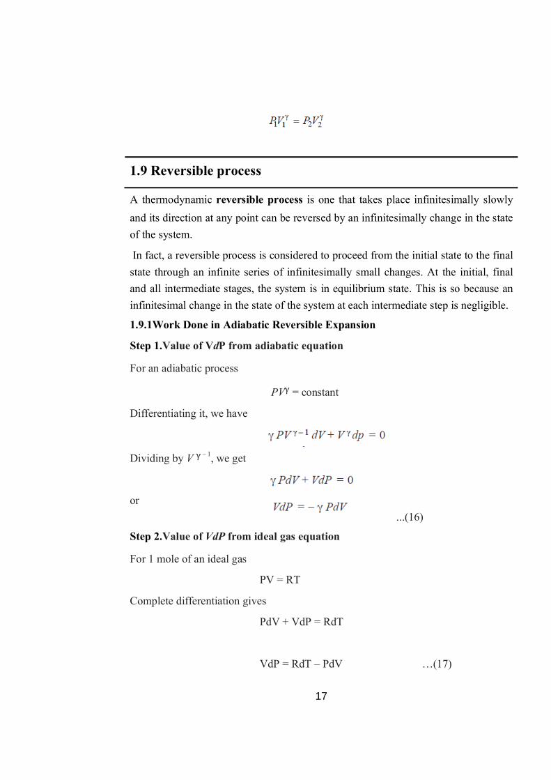
1.9.1Work Done in Adiabatic Reversible Expansion

Step 1.Value of VdP from adiabatic equation

For an adiabatic process

PVγ = constant

Differentiating it, we have

Dividing by V γ – 1, we get

or ...(16)

Step 2.Value of VdP from ideal gas equation

For 1 mole of an ideal gas

PV = RT

Complete differentiation gives

PdV + VdP = RdT

VdP = RdT – PdV …(17)

18

Step 3.Substitution

Substituting the value of VdP from (16) in (17) we get

RdT – PdV = – γPdV

or

RdT = P (1 – γ) dV

or

If there are n moles of a gas

Step 4.Integration

Integrating from T1, V1 to T2, V2 with γ constant

When T2 >T1, wmaxis negative because 1 – γ is negative. This means that work is done on the gas. On the other hand, when T2 <T1, wmax is positive which means that work is done by the gas.

SOLVED PROBLEM. Calculate w for the adiabatic reversible expansion of 2 moles of an ideal gas at 273.2 K and 20 atm to a final pressure of 2 atm.

SOLUTION

Given

Cp = 5R/2, mole–1deg–1

19

Cv= 3R/2, mole–1deg–1

R = 8.314J mole–1deg–1

Step 1.To calculate the value of T2, the final temperature, using the equation

(T2 / T1)γ = (P2 / P1)γ – 1

Substituting the value of γ in above equation

(T2 / 273.2)5/3 = (2 / 20)

Solving it, we get

T2 = 108.8 K

Step 2.To calculate maximum work under adiabatic conditions

= 4100 J = 4.1 kJ

ALTERNATIVE SOLUTION

The work done under adiabatic conditions may be obtained by calculating decrease in internal energy.

w = – ΔE = – nCv (T2 – T1)

= – 2 × 3 / 2 × 8.314 (108.8 – 273.2)

= 4100 J = 4.1 KJ

1.3 Complete the following statements

a) For adiabatic process, ^E =

b) An infinitesimal change in reversible process at each intermediate step is

……….

20

c) When T2 > T1 ; W maa = …………………….

d) Relation between temperature and volume with heat capacities is given by

which equation?


When a process goes from the initial state to the final state in a single step and cannot be carried in the reverse order, it is to be an irreversible process.

Here the system is in equilibrium state in the beginning and at the end, but not at points; in between. Most of the processes are irreversible in nature. Flow of heat from high temperature to low temperature, water flowing from -hill, expansion of gas from higher to lower pressure, use of cells or batteries directly are few example of irreversible process. They are also called spontaneous process.

1.10.1 Work Done In Adiabatic Irreversible Expansion

There are two type of irreversible expansion, namely

(1) Free expansion

(2) intermediate expansion

(1) Free expansion

In a free expansion we have Pext. = 0

So δw = Pext. . dV = 0

Also E =δq - δw

E = 0 - 0 = 0

Since for an ideal gas E = (T), it follows that the temperature of the gas remain unchanged, now

H =E + d(PV)

H =E + d(nRT)

H =E + nRdT

= 0 + 0

21

(dT = 0)

Thus all the quantities w, q, H and E are 0 for adiabatic free expansion of gas.

(2) Intermediate expansion

Here the work is done against a constant pressure and is given by

δw = Pext. . dV

on integrating above equation in the range of V1 and V2

w = Pext. (V2-V1)

= Pext. (nRT2/P2 - nRT1/P1)

If Pext. = P2 = the final pressure

Then w = P2(nRT2/P2 - nRT1/P1)

w = nRT1(T2/T1 - P2/P1)

Here T2 is the final temperature in adiabatic irreversible expansion and is different than that in the adiabatic reversible expansion.

In irreversible process more work is done by surrounding in bringing the system back to its original state than by the system during the forward reaction . So in cyclic transformation at constant temperature a net amount of work is destroyed in the surrounding. This process can be completed in finite time and are real process.

1.11Summary

In thermodynamics, a state function or state variable is a property of a system that depends only on the current state of the system, not on the way in which the system acquired that state (independent of path). A state function describes the equilibrium state of a system. For example, internal energy, enthalpy, and entropy are state quantities.

If dF is an exact differential, integration of this will be the same for all paths between the initial state and final state .Thermodynamic state functions, like U and H, should have exact differentials.

If dF an inexact differential, it will depend on the path which is used between the initial state and final state. Functions with inexact differentials cannot be treated as thermodynamic state functions.

22

The internal energy is neither possible nor necessary to calculate the absolute value of internal energy of a system. In thermodynamics we are concerned only with the energy changes when a system changes from one state to another.

The temperature dependence of Internal Energy U and Enthalpy H can be related to heat capacities Cv and Cp.

The heat capacities are defined as the heat that must be supplied to raise the temperature by 10C.

The heat capacity at constant volume is defined as the rate of change of internal energy with temperature at constant volume. Heat capacity at constant pressure is defined as the rate of change of enthalpy with temperature at constant pressure.

A process carried in a vessel whose walls are perfectly insulated so that no heat can pass through them, is said to be adiabatic. In such a process q = 0.

Work Done In Adiabatic Reversible Expansion is

Work Done In Adiabatic Irreversible Expansion isn RT1(T2/T1 - P2/P1)

1.12 Glossary

System : Specified protein of matter in universe for study

Surrounding : Rate of the universe in a position to exchange energy and

matter with the system.

Boundary : System is separated from surrounding by a boundary which may

be red or imaginary.

Thermodynamics : Branch of science deals with heat and work in all types of

chemical and physical process.

Process : An operation by which a system changes from one state to another.

23

Answer to say assessment questions

1.1 a) Thermal (b) adialatree d) P (iv) V

1.2 a) T b) F c) F d) T

1.3 a) –W b) heg ligible c) hegative d) ln T2/T1 =(CP- CV)mV_


1. When 10-g lead slug is taken from a beaker of boiling water and dropped

into a beaker containing 100g of ice-temperature water, the temperature of

this 00C water rises by 0.310C. What does this study tell us about the molar heat capacity of lead? Specific heat capacity of water = 4.184 J g 0C.

2. Find E, q and w if 2 moles of hydrogen at 3 atm pressure expand isothermally at 50ºC and reversibly to a pressure of 1 atm.

3 Verify whether df=(21x2y+14y4)dx+(17x3+188xy3)dy is an exact differential or not.

4 1g of water at 373 K is converted into steam at the same temperature. The

volume of water becomes 1671 ml on boiling. Calculate the change in the internal energy of thesystem if the heat of vaporisation is 540 cal/g.

5. Three moles of an ideal gas (Cv = 5 cal deg–1 mol–1) at 10.0 atm and 0º are

converted to 2.0 atm at 50º. Find E and H for the change.

R = 2 cal mol–1 deg–1

6. For the amount n mole of an ideal gass derive the expression for following processes

1. Adiabatic reversible work expansion

2. . Adiabatic reversible work expansion

3. Internal Energy

7. Define or explain the following terms :

(a) First law of thermodynamics (b) Adiabatic reversible expansion

24

(c) Irreversible expansion (d) Internal energy

8. Derive the following relation for the ideal gas undergoing adiabatic reversible process

1. TVγ-1=Constant

2. PVγ= Constant Where γ=Cp/Cv

1.13 References and Suggested reading

1. Physical Chemistry - Thomas Engel and Philip Reid (Pearson Education) 2006

2. Physical Chemistry - Ira N. Levine (McGRAW-HILL), 1988

3. Thermodynamic for Chemist - Glasstone, Samuel.( Affiliated East West Press Pvt. Ltd.), 2001

4. Physical Chemistry - P. Atkins (Oxford University Press), 2006

25

Unit - 2 : Thermochemistry Structure of Unit

2.0 Objectives

2.1 Introduction

2.2 Thermodynamics Law

2.3 Gibbs-Helmholtz Equation

2.4 Endothermic & Exothermic Reactions

2.5 Concentrating on the system

2.6 Maximum work

2.7 Summery

2.8 Glossary




At the end of the unit learner will be able to

Familiar with Thermo chemistry.

Learn the Reversible and irreversible processes.

Understand about Thermodynamic Systems.

Increase knowledge about Maximum Work.

Familiar with Exothermic and Endothermic Reactions.

2.0 Objectives

26

Thermodynamics (from the Greek words for “heat” and “power”) is the study of heat, work, energy, and the changes they produce in the states of systems. In a broader sense, thermodynamics studies the relationships between the macroscopic properties of a system. A key property in thermodynamics is temperature; Thermodynamics is sometimes defined as the study of the relation of temperature to the macroscopic properties of matter. Simifarly equilibrium thermodynamics deals with systems in equilibrium. (Irreversible thermodynamics deals with non equilibrium systems and rate processes.) Equilibrium thermodynamics is a macroscopic science and is independent of any theories of molecular structure. Strictly speaking, the word “molecule” is not part of the vocabulary of thermodynamics. However, we won’t adopt a purist attitude but will often use molecular concepts to help us understand thermodynamics. Thermodynamics does not apply to systems that contain only a few molecules; a system must contain a great many molecules for it to be treated thermodynamically.

Thermodynamic Systems

The macroscopic part of the universe under study in thermodynamics is called the system. The parts of the universe that can interact with the system are called the surroundings.

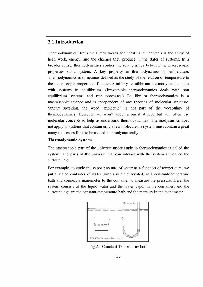
For example, to study the vapor pressure of water as a function of temperature, we put a sealed container of water (with any air evacuated) in a constant-temperature bath and connect a manometer to the container to measure the pressure. Here, the system consists of the liquid water and the water vapor in the container, and the surroundings are the constant-temperature bath and the mercury in the manometer.

Fig 2.1 Conetant Temperature both

2.1 Introduction

27

An open system is one where transfer of matter between system and surroundings can occur. A closed system is one where no transfer of matter can occur between system and surroundings. An isolated system is one that does not interact in any way with its surroundings. An isolated system is obviously a closed system, but not every closed system is isolated. For example, the system of liquid water plus water vapour in the sealed container is closed (since no matter can enter or leave) but not isolated (since it can be warmed or cooled by the surrounding bath and can be compressed or expanded by the mercury). For an isolated system, neither matter nor energy can be transferred between system and surroundings. For a closed system, energy but not matter can be transferred between system and surroundings. For an open system, both matter and energy can be transferred between system and surroundings. A thermodynamic system is either open or closed and is either isolated or non isolated. Most commonly, we shall deal with closed systems.

Equilibrium and non equilibrium states

An equilibrium state is, the state arrived at by an isolated system after an infinitely long period of time. For practical purposes equilibrium is reached in a finite time (the relaxation time) that depends on the nature of the bodies, their interactions, and the initial non-equilibrium state. If a system is in a state of equilibrium, then its individual macroscopic parts are also in a state of equilibrium. Under constant external conditions, such a state does not vary with time. Invariance in time, however, is not a sufficient criterion for a state to be an equilibrium state. If, for example, a section of an electric circuit through which a direct current flows is placed in a thermostat, or heat reservoir, the section can remain in an unchanging, or steady, state for a practically unlimited time. This state, however, is not an equilibrium state, since the flow of the current is accompanied by the irreversible conversion of the energy of the electric current into heat that is transferred to the thermostat. A temperature gradient is present in the system. Open systems may also be in a steady non equilibrium state.

The equilibrium state can be characterized completely by a small number of physical parameters. The most important of these parameters is temperature. For a system to be in thermodynamic equilibrium, all parts of the system must be at the same temperature. The existence of temperature—that is, a parameter that has the same value for all parts of a system in equilibrium—is often called the zeroth law of thermodynamics. The state of a homogeneous liquid or gas can be defined

28

completely by specifying any two of the following three quantities: the temperature T, volume V, and pressure p. The relation between p, V, and T is characteristic of each given liquid or gas and is called the equation of state. Examples are the equation of state for an ideal gas and vander Waals’ equation. In more complex cases other parameters—such as the concentrations of the individual components of a mixture of gases, electric field strength, and magnetic induction—may be required to characterize completely an equilibrium state.

Reversible (quasi-static) and irreversible processes

A system may undergo a change from one equilibrium state to another under the influence of various external factors. In this process the system passes through a continuous series of states that generally are non equilibrium states. A process must occur sufficiently slowly in order for its properties to approach those of an equilibrium process. Slowness, however, is not by itself a sufficient condition for an equilibrium process. For example, the process of the discharge of a capacitor across a high resistance or the process of throttling, wherein a pressure drop causes a gas to flow through a porous barrier from one vessel to another, may be arbitrarily slow and at the same time essentially non equilibrium processes. Since an equilibrium process is a continuous chain of equilibrium states, it is reversible; in other words, it can be performed in the reverse direction, so that both the system and the surroundings are restored to their original states. Thermodynamics provides a complete quantitative description of reversible processes. For irreversible processes, it establishes only certain inequalities and indicates the direction in which the processes occur.

Any physical system will spontaneously approach an equilibrium that can be described by specifying its properties, such as pressure, temperature, or chemical composition. If external constraints are allowed to change, these properties generally change. The three laws of thermodynamics describe these changes and predict the equilibrium state of the system. The first law states that whenever energy is converted from one form to another, the total quantity of energy remains the same. The second law states that, in a closed system, the entropy of the system does not decrease. The third law states that, as a system approaches absolute zero, further extraction of energy becomes more and more difficult, eventually becoming theoretically impossible.

29

First law of thermodynamics

The state of a system can be changed in two fundamentally different ways. In one way, the system does work on surrounding bodies so as to displace them over macroscopic distances, or work is performed by these bodies on the system. In the other way, heat is transferred to or from the system, and the positions of the surrounding bodies remain unchanged. In the general case the change of a system

from one state to another is associated with the transfer of some amount of heat ΔQ

to the system and with the performance of work ΔA by the system on external

bodies. When the initial and final states are specified, it was found that ΔQ and ΔA depend essentially on the path of the change of state. In other words, these quantities are characteristics not of an individual state of the system but of the process followed by the system. The first law of thermodynamics states that if a system follows a thermodynamic cycle (that is, ultimately returns to its initial state), then the total amount of heat transferred to the system over the course of the cycle is equal to the work performed by the system.

The first law of thermodynamics is essentially an expression of the law of conservation of energy for systems in which thermal processes play an important role. The energy equivalence of heat and work, that is, the possibility of measuring their quantities in the same units and thus the possibility of comparing them, was demonstrated in experiments carried out by J. R. von Mayer in 1842 and, especially, J. Joule in 1843. The first law of thermodynamics was formulated by Mayer; a much clearer formulation was provided by H. von Helmholtz in 1847. The statement of the first law given above is equivalent to the assertion that a perpetual motion machine of the first kind is impossible.

For a process where the system does not return to its initial state, it follows from the

first law that the difference ΔQ – ΔA = ΔU, which is in general nonzero, does not depend on the path between the initial and final states. In fact, any two processes occurring in opposite directions between the same end states form a closed cycle for

which the indicated difference vanishes. Thus, ΔU is the change in the quantity U,

2.2 Thermodynamics Laws

30

which has a well-defined value in every state and is said to be a function of state, or state variable, of the system. The quantity U is called the internal energy, or simply the energy, of the system. The first law of thermodynamics thus implies that there exists a characteristic function of the state of a system, its internal energy. In the case of a homogeneous body which is capable of performing work only upon a change in

volume, we have ΔA = pdV and the infinitesimal increment (differential) of U is given as follows-

(1) dU = dQ – pdV

Here, dQ is an infinitesimal increment of heat; it is not, however, a differential of some function. For a fixed volume (dV = 0), the heat supplied to the body goes to an increase in internal energy. The heat capacity of a body at constant volume is therefore cv = (dU/dT). Another state function is the enthalpy H = U + pV with the differential

dH = dU + V dp

The introduction of enthalpy makes it possible to obtain an expression for heat capacity measured at constant pressure, cp = (dH/dT)p. In the case of an ideal gas, which is described by the state equation pV = nRT (where n is the number of moles of the gas in a volume V and R is the gas constant), both the free energy and the enthalpy of a certain mass of the gas depend only on T. This assertion is confirmed, for example, by the absence of cooling in the Joule-Thomson process. Therefore, for an ideal gas cp – cV = nR.

Second law of thermodynamics: The first law of thermodynamics does not exclude the possibility of constructing a continuous-operation machine that would be capable of converting into useful work practically all of the heat supplied to it. Such a device is called a perpetual motion machine of the second kind. Nevertheless, all the experience in designing heat engines that had been amassed by the early 19th century indicated that the efficiency of heat engines (the ratio of the heat expended to the work obtained) is always considerably less than unity, some of the heat is unavoidably dissipated to the surroundings. S. Carnot showed in 1824 that this fact is fundamental in character that is, any heat engine must contain not only a heat source and a working substance, such as steam, that undergoes a thermodynamic cycle but also a heat sink whose temperature must be lower than that of the heat source.

31

In the second law of thermodynamics Carnot’s conclusion is generalized to arbitrary thermodynamic processes occurring in nature. In 1850, R. Clausius formulated the second law in the following way.

Heat cannot spontaneously pass from a system at a lower temperature to a system at a higher temperature. In 1851, W. Thomson (Lord Kelvin) set forth, independently, a slightly different statement of the law. It is impossible to construct a periodically operating machine whose activity reduces entirely to the raising of some load (the performance of mechanical work) and the corresponding cooling of a heat reservoir. Despite the qualitative character of this assertion, it has far-reaching quantitative consequences. For example, it permits the maximum efficiency of a heat engine to be determined.

Suppose a heat engine operates in a Carnot cycle. When the working substance is in isothermal contact with the heat source (T = T1), the working substance receives the

quantity of heat ΔQ1. In the other isothermal process of the cycle, where the working substance is in contact with the heat sink (T = T2), the working substance gives up the

quantity of heat ΔQ2. The ratio ΔQ2/ΔQ1 cannot depend on the nature of the working substance and must be the same for all heat engines operating in a reversible Carnot cycle that have the same heat-source temperature and the same heat-sink temperature. If the opposite were the case, then an engine with a smaller ratio could be used to drive an engine with a larger ratio in the reverse direction (since the cycles are reversible). In this combined engine heat from the heat sink would be transferred to the heat source without the performance of work. Since this situation violates the

second law of thermodynamics, the ratio ΔQ2/ΔQ1 must be the same for both engines. In particular, it must be the same as in the case in which the working substance is an ideal gas. This ratio can be easily found. Thus, for all reversible Carnot cycles there holds the relation:

which is sometimes called Carnot’s proportion. As a result, for all engines with a

reversible Carnot cycle, the efficiency is at a maximum and is η = (T1 – T2)/T1. In the case of irreversible cycles, the efficiency is less than this quantity. It must be emphasized that Carnot’s proportion and the efficiency of a Carnot cycle have indicated form only when the temperature is measured on an absolute temperature

32

scale. Carnot’s proportion has been made the basis for determining the absolute temperature scale.

The existence of entropy as a function of state is a consequence of the second law of thermodynamics (Carnot’s proportion). Let us introduce a quantity S such that the

change in S upon an isothermal reversible transfer of the quantity of heat ΔQ to the

system is ΔS = ΔQ/T. The net change in S in Carnot cycle is zero; in the adiabatic

processes of the cycle, ΔS = 0 (since ΔQ = 0), and the changes in the isothermal processes compensate for each other. The net change in S also turns out to be zero for an arbitrary reversible cycle. This statement can be proved by dividing the cycle into a sequence of infinitely small Carnot cycles with infinitesimal isothermal portions. It follows, as in the case of internal energy, that the entropy S is a function of the state of the system; that is, the change in entropy does not depend on the path of the changing states. Using the concept of entropy, Clausius showed in 1876 that the original statement of the second law of thermodynamics is equivalent to the following: there exists a state function of a system, the system’s entropy S, Such that the change in S during a reversible transfer of heat to the system is given by :

dS = dQ/T

In real (irreversible) adiabatic processes, the entropy increases, reaching its maximum value at the state of equilibrium.

Third law of thermodynamics

In accordance with the second law of thermodynamics, entropy is defined by the

differential equation as dQdsT

. This equation determines entropy to an accuracy

of a constant term that is not dependent on temperature but could differ for different bodies in the equilibrium state. Thermodynamic potentials also have corresponding undefined terms. In 1906, W. Nernst concluded from electrochemical research, that these terms must be universal that is, they are independent of pressure, state of aggregation, and other characteristics of a substance. This new experimentally based principle is usually called the third law of thermodynamics, or the Nernst heat theorem In 1911, M. Planck showed that an equivalent statement of the principle is that the entropy of all bodies in equilibrium state tends toward zero as a temperature of absolute zero is approached, since the universal constant in entropy may be set equal to zero. It

33

follows in particular from the third law of thermodynamics that the coefficient of

thermal expansion, isochoric pressure coefficient (∂p/∂T)V, and heat capacities cp

and cV vanish as T→ 0.

It should be noted that the third law of thermodynamics and its consequences do not pertain to systems in meta stable states. An example of such a system is a mixture of substances between which chemical reactions are possible but are retarded because the reaction rates at low temperatures are very low. Another example is a rapidly frozen solution, which should separate into phases at a low temperature; in practice, however, the separation process does not occur at low temperatures. Such states are similar to equilibrium states in many regards, but their entropy does not vanish when T = 0.

Applications. Important areas of application of thermodynamics include the theory of chemical equilibrium and the theory of phase equilibrium, in particular, the theory of equilibrium between different states of aggregation and equilibrium upon the phase separation of mixtures of liquids and gases. In these cases, the exchange of particles of matter between different phases plays an important role in the establishment of equilibrium, and the concept of chemical potential is used in formulating the equilibrium conditions. Constancy of chemical potential replaces the condition of constancy of pressure if the liquid or gas is located in an external field, such as a gravitational field. The methods of thermodynamics are used effectively in the study of natural phenomena in which heat effects play an important role. In thermodynamics a distinction is commonly made between branches that pertain to individual sciences and engineering, such as chemical thermodynamics and engineering thermodynamics, and branches dealing with different objects of investigation, such as the thermodynamics of elastic bodies, of dielectrics, of magnetic media, of superconductors, of plasmas, of radiation, of the atmosphere, and of water.

The establishment of the statistical nature of entropy led to the construction of the thermodynamic theory of fluctuations by A. Einstein in 1910 and to the development of nonequilibrium thermodynamics.

2.1 Choose the connect alternative

a) Enthalpy is sum of

(i) U+PT (ii) U+PV (iii) P+UT) (iv) none

34

b) Cornot cycle says that

(i) ………..

C) Gibles free energy is related with entropy as

(i) G = H-TS (ii) G = T-Hs (iii) both (iv) all

d) When volume of system is constant then entropy change of surrounding tends to –

(i) Minimum (ii) Zero (iii) Maximum (iv) all

Derivation of the Gibbs-Helmholtz Equation

The Gibbs-Helmholtz equation provides information about the temperature dependence of the Gibbs free energy. The derivation of the Gibbs-Helmholtz equation begins with the fundamental equation for the Gibbs free energy G,

dG SdT VdP …(1)

Using the relationships for an exact differential, we have that

…(2)

Substituting this result for –S into the equation defining the Gibbs free energy, we get

G = H −TS …(3)

Dividing both sides of Eq. by T leads to the result

…(4)

2.3Gibbs-Helmholtz Equation

35

The Gibbs-Helmholtz equation involves the partial derivative with respect to temperature (at constant pressure) of the quantity on the left side of Eq, G/T . Taking the partial derivative gives

…(5)

Note that in Eq, since G is a function of temperature, G = G (T), the product rule was employed in order to evaluate the derivative of G/T. Factoring 1/T out from the right side of Eq. yields

…(6)

Substituting the relation for G/T from Eq. (4) gives the result Equation (7) provides one form of the Gibbs-Helmholtz equation.

…(7)

Another useful form of the Gibbs-Helmholtz equation may be obtained by considering the derivative

…(8)

36

The result in Eq. (8) may be derived by making the substitution u 1/T such that du

2

dtT

. Substituting the result for the partial derivative on the right from Eq. (7) leads to

the primary form for the Gibbs-Helmholtz equation.

…(9)

Written in terms of the change in free energy, the Gibbs-Helmholtz equation is

…(10)

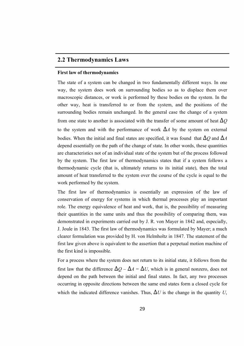
Exploring the Temperature Dependence of the Gibbs Free Energy Change

For an endothermic reaction, the slope of the Gibbs-Helmholtz equation given in Eq. (10) is positive, as illustrated in Figure 2.2.

Fig 2.2

2.4Endothermic & Exothermic Reactions

37

From Figure 2.2, we see that as the temperature increases (from right to left along the x-axis), the Gibbs free energy change decreases (as long as the final and initial temperatures are not too different from one another); that is,

For T final >Tinitial ,ΔGfinal <ΔGinitial . (11)

Note that if the Gibbs free energy change at the initial temperature was negative (indicating a spontaneous process), then increasing the temperature further decreases the Gibbs free energy change (in other words, the value becomes more negative).

For an exothermic reaction, the slope for the Gibbs-Helmholtz equation given in Eq. (10) is negative, as illustrated in Figure 2.3.

From Figure 2.3, we see that as the temperature increases (from right to left along the x-axis), the Gibbs free energy change also increases (as long as the final and initial temperatures are not too different from one another); that is

For T final >Tinitial ,ΔGfinal >ΔGinitial . (12)

Note in this case that if the Gibbs free energy change at the initial temperature is negative (indicating a spontaneous process), then increasing the temperature increases the Gibbs free energy change (in other words, the value becomes less negative).

38

Entropy is the basic concept for discussing the direction of natural change, but to use it we have to analyse changes in both the system and its surroundings. We have seen that it is always very simple to calculate the entropy change in the surroundings, and we shall now see that it is possible to devise a simple method for taking that contribution into account automatically. This approach focuses our attention on the system and simplifies discussions. Moreover, it is the foundation of all the applications of chemical thermodynamics that follow.

The Helmholtz and Gibbs energies

Consider a system in thermal equilibrium with its surroundings at a temperature T. When a change in the system occurs and there is a transfer of energy as heat between the system and the surroundings, the CIausius inequality equation holds good.

We can develop this inequality in two ways, according to the conditions (of constant volume or constant pressure) under which the process occurs.

(a) Criteria for spontaneity

First, consider heating at constant volume. Then, in the absence of non-expansion work, we can write dqv= dU.

The importance of the inequality in this form is that it expresses the criterion for spontaneous change solely in terms of the state functions of the system. The inequality is easily rearranged to

TdS 2':dU (constant V, no additional work)

At either constant internal energy (dU = 0) or constant entropy (dS = 0), this expression expresses the criteria for spontaneous change in terms of properties relating to the system. The first inequality states that, in a system at constant volume and constant internal energy (such as an isolated system), the entropy increases in a spontaneous change. That statement is essentially the content of the Second Law. The second inequality is less obvious, for it says that, if the entropy and volume of the system are constant, then the internal energy must decrease in a spontaneous change. Do not interpret this criterion as a tendency of the system to sink to lower energy. It is a disguised statement about entropy, and should be interpreted as implying that, if the entropy of the system is unchanged, then there must be an

2.5 Concentrating on the system

39

increase in entropy of the surroundings, which can be achieved only if the energy of the system decreases as energy flows out as heat. When energy is transferred as heat at constant pressure, and there is no work other than expansion work, we can write dqp = d.H and obtain.

TdS ≥dH (constant p, no additional work)

At either constant enthalpy or constant entropy this inequality becomes, respectively,

dSH,p ≥ 0

dHs,p≤0

The entropy of the system at constant pressure must increase if its enthalpy remains constant (for there can then be no change in entropy of the surroundings). Alternatively, the enthalpy must decrease if the entropy of the system is constant, for then it is essential to have an increase in entropy of the surroundings. As are know that

dU – TdS≤ 0 and dH – TdS≤ 0, respectively,

they can be expressed more simply by introducing two more thermodynamic quantities. One is the Helmholtz energy, A, which is defined as

A= U-TS …………(13)

The other is the Gibbs energy, G:

G=H-TS …………(14)

All the symbols in these two definitions refer to the system. When the state of the system changes at constant temperature, the two properties change as follows:

(a) dA=dU-TdS

(b) dG= dH – TdS

We obtain the criteria of spontaneous change as

(A) dAT,V≤ 0

(b) dGT,p ≤ 0

These inequalities are the most important conclusions from thermodynamics for chemistry.

40

(b) Some remarks on the Helmholtz energy

A change in a system at constant temperature and volume is spontaneous if dAT,v≤o.

That is, a change under these conditions is spontaneous if it corresponds to a decrease in the Helmholtz energy. Such systems move spontaneously towards states of lower

Aif a path is available. The criterion of equilibrium, when neither the forward nor

reverse process has a tendency to occur, is

dAT,v= 0

The expressions dA=dU-TdS and dA < 0 are sometimes interpreted as follows. A negative value of dA is favoured by a negative value of dU and a positive value of TdS. This observation suggests that the tendency of a system to move to lower A is due to its tendency to move towards states of lower internal energy and higher entropy. However, this interpretation is false (even though it is a good rule of thumb for remembering the expression for dA) because the tendency to lower A is solely a tendency towards states of greater overall entropy. Systems change spontaneously if in doing so the total entropy of the system and its surroundings increases, not because they tend to lower internal energy. The form of dA may give the impression that systems favour lower energy, but that is misleading, dS is the entropy change of the system, -dU/T is the entropy change of the surroundings (when the volume of the system is constant), and their total tends to a maximum.

2.2 Fill in the blanks

a) For a spontaneous process &G = ……….

b) At a constant ----------we have tds>dH.

c) In endo thermic reactions heat is ……………

d) Gibbes hemlatz reaction is ……………

It turns out that A carries a greater significance than being simply a signpost of spontaneous change, the change in the Helmholtz function is equal to the maximum work accompanying a process, dwmax=dA

2.6Maximum work

41

As a result, A is sometimes called the 'maximum work function', or the 'work function'. To demonstrate that maximum work can be expressed in terms of the

changes in Helmholtz energy, we combine the Clausius inequality dS ≥ dq/T in the

form TdS≥ dq with the First Law, dU = dq + dw, and obtain

dU≤TdS+dw

(dU is smaller than the term on the right because we are replacing dq by TdS, which

in general is larger.) This expression rearranges to dW≥dU- TdS

It follows that the most negative value of dw, and therefore the maximum energy that can be obtained from the system as work, is given by

dwmax = dU – TdS

and that this work is done only when the path is traversed reversibly (because then the equality applies). Because at constant temperature dA = dU - TdS,we conclude that

dwmax = dA.

When a macroscopic isothermal change takes place in the system, eqn becomes

Wmax" =M

With A=U-TS

This expression shows that in some cases, depending on the sign of TS, not all the change in internal energy may be available for doing work. If the change occurs with

a decrease in entropy (of the system), in which case TS < 0, then the right-hand

side of this equation is not as negative as U itself, and consequently the maximum

work is less than U. For the change to be spontaneous, some of the energy must escape as heat in order to generate enough entropy in the surroundings to overcome the reduction in entropy in the system. In this case, nature is demanding a tax on the internal energy as it is converted into work. This is the origin of the alternative name

'Helmholtz free energy' for A because A is that part of the change in internal energy that we are free to do work.

If the change occurs with an increase of entropy of the system (in which case TS> 0), the right-hand side of the equation is more negative than flU. In this case, the maximum work that can be obtained from the system is greater than U. The

42

explanation of this apparent paradox is that the system is not isolated and energy may flow in as heat as work is done. Because the entropy of the system increases, we can afford a reduction of the entropy of the surroundings yet still have, overall, a spontaneous process. Therefore, some energy may leave the surroundings as heat and contribute to the work the change is generating

2.7 Summary

This Chapter increases the knowledge of Thermochemistry, and this Chapter also explains brief about Thermodynamics study of heat, work, energy, and the changes they produce in the states of systems and as well as be studying equilibrium thermodynamics, which deals with systems in equilibrium. (Irreversible thermodynamics deals with non equilibrium systems and rate processes.).

2.8 Glossary

Exothermic reaction: Energy is liberated during reactions.

Endothermic reaction : Energy is absorbed during reaction.

Entropy : Randomness in system

Closed System : System which can not transfer matter but co transfer energy in

from of heat, work.

Dependent variable : whose value depend on value of P and T.


2.1 a) … b) ; c) (i) d) (iii)

2.2 (a) –he b) P c) liberated o(G/T) = OH

2.9 Review Question

1. Define Thermochemistry? 2. What is 'Maximum work function'?

43

3. What is Gibbs-Helmholtz Equation? 4. Define the Concentrating on the system? 5. Explain Thermodynamics Law?


1. Atkins Physical Chemistry (Peter Atkins& Julio de Paula 8th Edition) 2. IRA N. LEVINE Physical Chemistry 6thEdition

44

Unit-3 : The Third Law of Thermodynamics Structure of unit

3.1 Objectives

3.2 Introduction

3.3 Basic concept of Entropy

3.4 Demerits of Entropy

3.5 Steric Factor

3.6 Gibb’s function

3.7 Molar Gibb’s function

3.8 Difference between entropy and Gibb's function

3.9 Summary

3.10 Glossary

3.11 References and Suggested Readings


3.12 Review Questions

3.1 Objectives

At the end of the chapter, student will be able to :

Explains how chemical reaction occurs

Know that Entropy was the first by which thermo chemistry of a chemical reaction was explained. That’s why Entropy is supposed to study first than any other theory or concept.

Understand importance of III low of themodynamuis.

45

3.2 Introduction

This chapter basically deals with the Entropy. One can understand following topics by study the chapter:

Basic concept of Entropy and its demerits

Importance of Steric factor for a chemical reaction

Gibb’s function, its limitations and applications

Molar Gibb’s function and its difference from Arrhenius equation

The third law of thermodynamics is sometimes stated as follows, regarding the properties of systems in equilibrium at absolute zero temperature.

The entropy of a perfect crystal, at absolute zero kelvin, is exactly equal to zero.

At zero kelvin the system must be in a state with the minimum possible energy, and this statement of the third law holds true if the perfect crystal has only one minimum energy state. Entropy is related to the number of possible microstates, and for a system containing a certain collection of particles. Quantum mechanics indicates that there is only one unique state (called the ground state) with minimum energy. If the system does not have a well-defined order (if its order is glassy, for example), then in practice there will remain some finite entropy as the system is brought to very low temperatures. The constant value is called the residual entropy of the system.

The Nernst-Simon statement of the third law of thermodynamics is in regard to thermodynamic processes, and whether it is possible to achieve absolute zero in practice.

The entropy change associated with any condensed system undergoing a reversible isothermal process approaches zero as temperature approaches 0 K. A simpler formulation of the Nernst-Simon statement might be: That it is impossible for any process, (no matter how idealized), to reduce the entropy of a system to its absolute-zero value in a finite number of operations.

Physically, the Nernst-Simon statement implies that it is impossible for any procedure to bring a system to the absolute zero of temperature in a finite number of steps.

46

3.3 Entropy and Gibb’s function

In thermodynamics, entropy (usual symbol S) is a measure of the number of specific ways in which a thermodynamic system may be arranged, often taken to be a measure of disorder, or a measure of progressing towards thermodynamic equilibrium. The entropy of an isolated system never decreases, because isolated systems spontaneously evolve towards thermodynamic equilibrium, which is the state of maximum entropy.

The change in entropy (ΔS) was originally defined for a thermodynamically reversible process as

which is found from the uniform thermodynamic temperature (T) of a closed system dividing an incremental reversible transfer of heat into that system (dQ). The above definition is sometimes called the macroscopic definition of entropy because it can be used without regard to any microscopic picture of the contents of a system. In thermodynamics, entropy has been found to be more generally useful and it has several other formulations. Entropy was discovered when it was noticed to be a quantity that behaves as a function of state, as a consequence of the second law of thermodynamics. Entropy is an extensive property, but the entropy of a pure substance is usually given as an intensive property — either specific entropy (entropy per unit mass) or molar entropy (entropy per mole).

The absolute entropy (S rather than ΔS) was defined later, using either statistical mechanics or the third law of thermodynamics.

In the modern microscopic interpretation of entropy in statistical mechanics, entropy is the amount of additional information needed to specify the exact physical state of a system, given its thermodynamic specification. Understanding the role of thermodynamic entropy in various processes requires understanding how and why that information changes as the system evolves from its initial condition. It is often said that entropy is an expression of the disorder, or randomness of a system, or of our lack of information about it. The second law is now often seen as an expression of the fundamental postulate of statistical mechanics via the modern definition of entropy. Entropy has the dimension of energy divided by temperature, which has a unit of joules per kelvin (J/K) in the International System of Units.

47

Generally, rate of a reaction is expressed in terms of a rate constant multiplied by a function of concentrations of reactants. As a result, it is the rate constant that contains information related to the collision frequency, which determines the rate of a reaction in the gas phase. When the rate constant is given by the Arrhenius equation,

Ea is related to the energy barrier over which the reactants must pass as products form. For molecules that undergo collision, the exponential is related to the number of molecular collisions that have the required energy to induce reaction. The pre-exponential factor, A, is related to the frequency of collisions. Therefore, we can describe the reaction rate as

Rate = (Collision frequency) x (Fraction of collisions with at least the threshold energy)

or

where Z is the frequency of collisions between molecules of A and B and F is the fraction of those collisions having sufficient energy to cause reaction.

The collision frequency between two different types of molecules can be calculated by means of the kinetic theory of gases. In this discussion we will consider the molecules of B as being stationary and A molecules moving through a collection of them. If we imagine a molecule of A moving through space where molecules of B are located, collisions will occur with molecules of B whose centers lie within a cylinder of length vAB and radius rA + rB where V1sj is the average relative velocity of A and B and rA + rB is the sum of the radii of molecules A and B. A diagram showing this situation is shown in the following figure 3.1.

Fig 3.1 Callision between A and B molecules

48

If the cross sectional area of the cylinder, π(rA + rB)2, the collisional cross section,

σAB In 1 second, a molecule of A travels a distance of vAB (where vAB is the average molecular velocity of A relative to B) and it will collide with all molecules of B that have centers that lie within the cylinder. Therefore, the number of collisions per second will be given by the number of B molecules/cm multiplied by the volume of the cylinder. This can be expressed by the equation

Although A does not continue in a straight line after colliding with B, the calculated collision frequency will still be correct as long as there is no gradient in concentration of B within the container and the velocity of A remains constant. The preceding result is for a single molecule of A. To obtain the total number of collisions between molecules of A and B, Z, the result must be multiplied by CA, the number of molecules of A per cm. Therefore, the collision frequency is

The analysis which led to the concept of entropy began with the work of French mathematician Lazare Carnot who in his 1803 paper Fundamental Principles of Equilibrium and Movement proposed that in any machine the accelerations and shocks of the moving parts represent losses of moment of activity. In other words, in any natural process there exists an inherent tendency towards the dissipation of useful energy. Building on this work, in 1824 Lazare's son Sadi Carnot published Reflections on the Motive Power of Fire which posited that in all heat-engines whenever "caloric", or what is now known as heat, falls through a temperature difference, work or motive power can be produced from the actions of the "fall of caloric" between a hot and cold body. He made the analogy with that of how water falls in a water wheel. This was an early insight into the second law of thermodynamics. Carnot based his views of heat partially on the early 18th century "Newtonian hypothesis" that both heat and light were types of indestructible forms of matter, which are attracted and repelled by other matter, and partially on the contemporary views of Count Rumford who showed (1789) that heat could be created by friction as when cannon bores are machined. Carnot reasoned that if the body of the working substance, such as a body of steam, is returned to its original state at the end of a complete engine cycle, that "no change occurs in the condition of the working body".

49

The first law of thermodynamics, formalized based on the heat-friction experiments of James Joule in 1843, deals with the concept of energy, which is conserved in all processes; the first law, however, is unable to quantify the effects of friction and dissipation.

In the 1850s and 1860s, German physicist Rudolf Clausius objected to the supposition that no change occurs in the working body, and gave this "change" a mathematical interpretation by questioning the nature of the inherent loss of usable heat when work is done, e.g. heat produced by friction. Clausius described entropy as the transformation-content, i.e. dissipative energy use, of a thermodynamic system or working body of chemical species during a change of state. This was in contrast to earlier views, based on the theories of Isaac Newton, that heat was an indestructible particle that had mass.

Later, scientists such as Ludwig Boltzmann, Josiah Willard Gibbs, and James Clerk Maxwell gave entropy a statistical basis. In 1877 Boltzmann visualized a probabilistic way to measure the entropy of an ensemble of ideal gas particles, in which he defined entropy to be proportional to the logarithm of the number of microstates such a gas could occupy. Henceforth, the essential problem in statistical thermodynamics, (i.e. according to Erwin Schrödinger) has been to determine the distribution of a given amount of energy E over N identical systems.

Because we have considered molecules of B to be stationary (velocity = 0), the relative velocity is just the root-mean-square velocity of A,

where T is the temperature (K), k is Boltzmann’s constant, and m is the mass of A. Note that Boltzmann’s constant is denoted in bold to distinguish it from a rate

constant. If we represent the reduced mass of a pair of molecules A and B as μ, then

or, in the more familiar form,

The relative velocity of A and B can now be written as

50

Having derived an expression for the relative velocity of the molecules, the collision frequency is expressed as

Frequently, the collision diameter, d = (dA + dB)/2, is used and the concentrations are written in terms of numbers of molecules/cm3, nA and nB, per unit volume. Then,

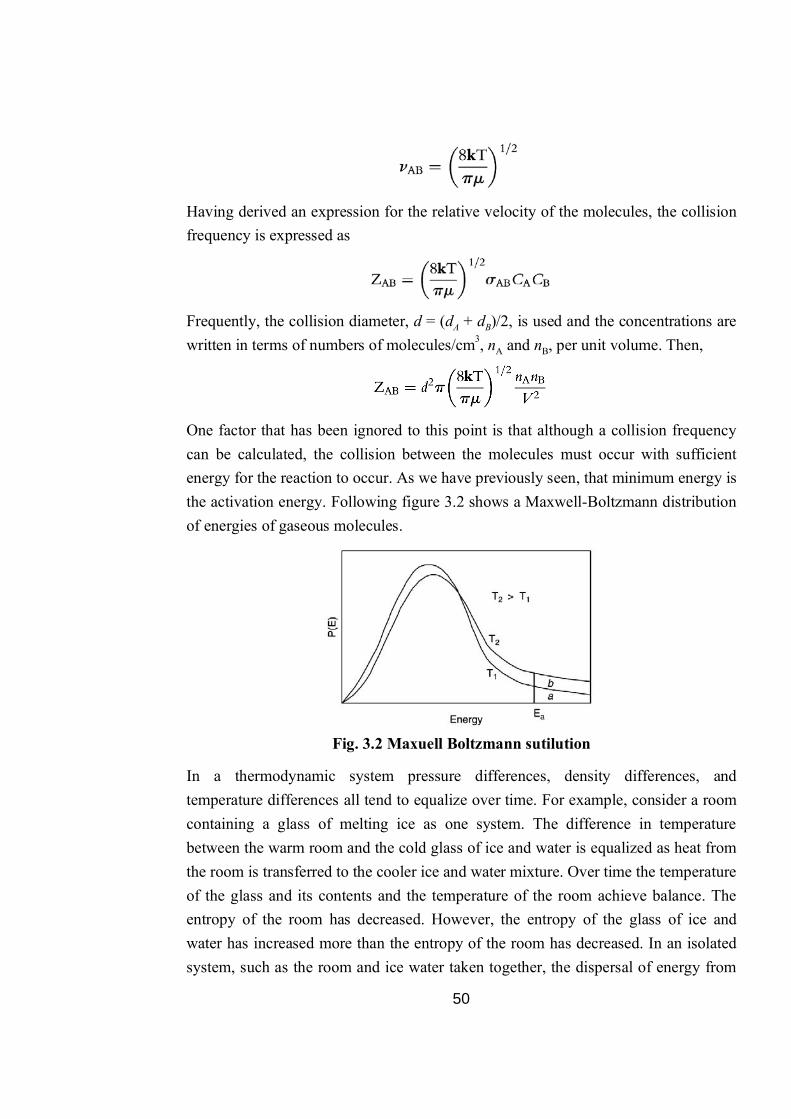
One factor that has been ignored to this point is that although a collision frequency can be calculated, the collision between the molecules must occur with sufficient energy for the reaction to occur. As we have previously seen, that minimum energy is the activation energy. Following figure 3.2 shows a Maxwell-Boltzmann distribution of energies of gaseous molecules.

Fig. 3.2 Maxuell Boltzmann sutilution

In a thermodynamic system pressure differences, density differences, and temperature differences all tend to equalize over time. For example, consider a room containing a glass of melting ice as one system. The difference in temperature between the warm room and the cold glass of ice and water is equalized as heat from the room is transferred to the cooler ice and water mixture. Over time the temperature of the glass and its contents and the temperature of the room achieve balance. The entropy of the room has decreased. However, the entropy of the glass of ice and water has increased more than the entropy of the room has decreased. In an isolated system, such as the room and ice water taken together, the dispersal of energy from

51

warmer to cooler regions always results in a net increase in entropy. Thus, when the system of the room and ice water system has reached temperature equilibrium, the entropy change from the initial state is at its maximum. The entropy of the thermodynamic system is a measure of how far the equalization has progressed.

There are many irreversible processes that result in an increase of the entropy. One of them is mixing of two or more different substances. The mixing is accompanied by the entropy of mixing. If the substances originally are at the same temperature and pressure, there will be no net exchange of heat or work in many important cases, such as mixing of ideal gases. The entropy increase will be entirely due to the mixing of the different substances.

From a macroscopic perspective, in classical thermodynamics, the entropy is a state function of a thermodynamic system, that is, a property depending only on the current state of the system, independent of how that state came to be achieved. Entropy is a key ingredient of the Second law of thermodynamics, which has important consequences e.g. for the performance of heat engines, refrigerators, and heat pumps.

We now consider inhomogeneous systems in which internal transformations (processes) can take place. If we calculate the entropy S1 before and S2 after such an

internal process, the Second Law of Thermodynamics demands that S2 ≥ S1 where the equality sign holds if the process is reversible. The difference Si = S2 - S1 is the entropy production due to the irreversible process. The Second law demands that the entropy of an isolated system cannot decrease.

Suppose a system is thermally and mechanically isolated from the environment (isolated system). For example, consider an insulating rigid box divided by a movable partition into two volumes, each filled with gas. If the pressure of one gas is higher, it will expand by moving the partition, thus performing work on the other gas. Also, if the gases are at different temperatures, heat can flow from one gas to the other provided the partition allows heat conduction. Our above result indicates that the entropy of the system as a whole will increase during these processes. There exists a maximum amount of entropy the system may possess under the circumstances. This entropy corresponds to a state of stable equilibrium, since a transformation to any other equilibrium state would cause the entropy to decrease, which is forbidden. Once the system reaches this maximum-entropy state, no part of

52

the system can perform work on any other part. It is in this sense that entropy is a measure of the energy in a system that cannot be used to do work.

An irreversible process degrades the performance of a thermodynamic system, designed to do work or produce cooling, and results in entropy production. The entropy generation during a reversible process is zero. Thus entropy production is a measure of the irreversibility and may be used to compare engineering processes and machines.

3.4 Demerits of Entropy

The demerits of Entropy are as follows,

1. Entropy does not provide any prediction of p, the “steric factor”. 2. The Entropy outlined above does not account for orientation of the collision,

front-to-back and along the line-of-centers. That is, molecules need to collide in the correct orientation for reaction to occur.

3. The Entropy does not explain the observed temperature dependence given by Arrhenius equation

4. Entropy assumes all A molecules have the same relative velocity, the average one.

5. Calculated values for the rate constant are usually too high compared with measured values.

6. Measured activation energies are lower than the energies of the bonds that have to be broken in reactions.

3.1 Chose the corcet atternative

a) Entropy is a measue of

(i) Disorder (ii) randomness (iii) both (iv) none

b) Rate of reaction is due to fruition of collision with

(i) Collision frequency (ii) temperature (iii) radii of molecule (iv) none

c) Entropy does not provide prediction of

(i) tempenture (ii) terice factor (iii) both (iv) none

d) Entropy generation during reversible process is

(i) Maximum (ii) minimum (iii) both (iv) zero

53

3.5 The third law of thermodynamics

As we know the Arrhenius equation is

In this equation A is sometimes referred to as the pre-exponential factor.

Estimates of EA can be made using experimental values of rate constants determined at different temperatures. Or, if the activation energy is known, its value can be used to predict rate constants at new temperatures. Also, the natural logarithm of Arrhenius equation can be taken to generate a new form of the equation:

Here, the labels indicate how this form of the Arrhenius equation is written in the form of a straight line. Pre-exponential factors and activation energies can be estimated graphically.

Above equation can also be written as;

which eliminates the need to know the pre-exponential factor A.

For some reactions, using the Van’t Hoff equation as the starting point to develop the Arrhenius equation is a little simplistic. Rather than assuming that

By including the temperature term, above equation becomes

or

For m = 0, above equation reduces into the Arrhenius equation.

54

The pre-exponential factor, which is a constant for a given reaction must have a value that is dictated by the specifics of the reaction itself, like the nature of the reactants and how they interact on a molecular level.

One of the most obvious is the number of molecules that are colliding. The number of collisions is calculable from kinetic theory. For example, at the end of that section we showed that the total number of collisions per second per unit volume, represented by Z, is given by

whered1 and d2 are the diameters of gas particles in species 1 and 2, and μ is the reduced mass of two particles of those species. If the effect of temperature changes is minor, compared to the exponential term in the Arrhenius equation (that is, the -EA/RTe

term), and if the densities of the two species ρ1 and ρ2 are converted to concentrations and separated from the rest of the expression, then it can be assumed that the rest of the expression is approximately constant, i. e.

This one factor, a collision frequency factor, is one major contribution to the pre-exponential constant A.

A second contribution to the value of A is the orientation of the two reactant species with respect to each other, and what fraction of collisions are oriented properly so that bond rearrangement might occur. The figure 3.3 shown effectively describes that how we can argue for a steric factor as a contribution to the pre-exponential factor A.

55

Fig. 3.3 Effect of steric petor

In the condition (a), the atoms are not arranged properly at the time of collision. In the condition (b), orientation factors are more favorable, and the reaction might proceed. Steric factors include not just the size of the collisional cross section but also considerations of reactant structure and geometry. This description of simple chemical reactions is called Entropy and is a basic theoretical model of the kinetics of chemical reactions.

3.6 Gibb’s function

A Entropy of even gas phase reactions is not totally satisfactory, and the problems with the steric factor that we described earlier make this approach more empirical and qualitative than we would like. Henry Eyring develops, somewhat different approach for Gibb’s function (or activated complex theory) refers to the details of how reactions become products. For a reaction like

AB + C → BC + A

it is assumed that there is a variation in potential energy which is related to atomic coordinates by an appropriate potential energy function. The term phase space is applied to the coordinate and momentum space for the system. For a reaction to occur, the transition state must pass through some critical configuration in this space. Because of the nature of the potential function used to express the energy of the system as a function of atomic positions, the system energy possesses a saddle point.

56

This saddle point lies lower in energy than the fully dissociated arrangement, A + B + C, or the highly “compressed” arrangement, A-B-C.

The main feature of Gibb’s function is that there is a “concentration” of the species at the saddle point, the transition state or activated complex, that is in equilibrium with reactants and products. The Boltzmann Distribution Law governs the concentration of that transition state, and the rate of reaction is proportional to its concentration. The concentration of the transition state is small because of its energy being higher than that of the reactants, hence this critical configuration represents the “regulator” of the rate of flow of reactants to products.

The concentration of the transition state is one of the factor which is involved, since the frequency of its dissociation into products comes into play because the rate at which it decomposes must also be considered. Therefore, the rate can be expressed as

Rate = (Concentration of Transition state) x (Decomposition frequency)

To form a product by the transition state, one bond must acquire sufficient vibrational energy to separate. When it does separate, one of the 3N — 6 vibrational degrees of freedom (for a linear molecule it is 3N — 5) is lost and is transformed into translational degrees of freedom of the products. The main idea of Gibb’s function is the assumption that the transition state species is in equilibrium with the reactants. Thus,

For the formation of the transition state, the equilibrium constant is

from which we find that the concentration of the transition state is

Since the reaction rate is expressed as the product of the concentration of the transition state and the frequency of its decomposition, we can now write

………..(1)

As we know that

57

And since

Therefore, the equilibrium constant for formation of the transition state can be written as

By putting this value in the equation (1), we get

Now we have obtained an expression for the rate in terms of concentrations and thermodynamic quantities, the frequency of decomposition of transition state must now be addressed.

By considering the vibration of the transition state when it is at the top of the potential energy barrier, temperature limit in energy for a vibrational mode can be expressed as

Where k is Boltzmann’s constant and T is the temperature (K). Since k = R/No (where No is Avogadro’s number), hence

Now since,

or

…………...…………….. (2)

Because the reaction rate can be expressed in terms of the concentration of the transition state, the rate can now be given by

Substituting for the rate constant gives

58

Now putting the value of equation (2) in the above equation

The rate constant can now be written as

A somewhat more elegant approach to deriving an expression for the rate of passage over the potential energy barrier is based on statistical mechanics. According to this method, it is assumed that there is a some distance, d, at the top of the barrier, which must be the distance where the transition state exists. It is the distance in which vibrational mode of the complex is transformed into translational motion of the products. The rate of passage of the transition state through distance d is related to the molecular velocity in one direction. If the mass of the transition state is m‡, the average velocity is

or

The number of complexes crossing the potential barrier through distance d per unit time is

Note that we are using []‡ to represent the transition state and [‡] to represent the concentration of the transition state. Now, the concentration of the transition state, [‡], is to be evaluated. If the difference between energies of the zero—point of the reactants and the transition state is Eo

‡, the equilibrium constant for formation of the transition state is given by

59

where QA,OB, and Q‡ are the partition functions of reactants A and B and the transition state, respectively. If the vibrational mode of the transition state is factored out of Q we can write

where q‡

v is the vibrational mode of the bond being broken. Now we can approximate the vibrational mode as

and the equilibrium constant K‡ is given by

which is of the same form found earlier with the rate constant, k, being given by

The resemblance of this equation to the Arrhenius equation is apparent when the pre-exponential factor includes the frequency factor and the equihbrium constant in terms of partition functions. This expression for k is similar to that obtained from Entropy.

An approximate rate constant, ka, can be calculated from probability that the reactants in the distribution of quantum state will collide and react in accord with the collision frequency. The approximate constant is greater than the measured rate constant, k. One approach to improving Gibb’s function with respect to calculating the rate constant is to alter the configuration of the transition state used in the energy calculations in order to effect a change in a. In fact, the calculations are performed in such a way that the calculated rate constant is a minimum and thereby approaches the observed k. Just as energy minimization is accomplished by means of the variation method in quantum mechanical calculations, this procedure is referred to in this connection as variational Gibb’s function.

Because the free energy of activation is given by

60

this procedure amounts to configuration optimization to minimize K‡ or maximize

G‡. In practice, a series of transition states is considered and the calculations are performed to obtain the desired minimization. It is of some consequence to choose the reaction path with respect to the energy surface.

Limitations of Gibb’s function

In general, Gibb’s function has provided researchers with a conceptual foundation for understanding how chemical reactions take place. Even though the theory is widely applicable, it does have limitations. For example, when applied to each elementary step of a multi-step reaction, the theory assumes that each intermediate is long-lived enough to reach a Boltzmann distribution of energies before continuing to the next step. When the intermediates are very short-lived, however, then TST fails. In such cases, the momentum of the reaction trajectory from the reactants to the intermediate can carry forward to affect product.

It is based on the assumption that atomic nuclei behave according to classic mechanics. It is assumed that unless atoms or molecules collide with enough energy to form the transition structure, then the reaction does not occur. However, according to quantum mechanics, for any barrier with a finite amount of energy, there is a possibility that particles can still tunnel across the barrier. With respect to chemical reactions this means that there is a chance that molecules will react even if they do not collide with enough energy to traverse the energy barrier. While this effect is expected to be negligible for reactions with large activation energies, it becomes a more important phenomenon for reactions with relatively low energy barriers, since the tunneling probability increases with decreasing barrier height.

Gibb’s function fails for some reactions which occur high temperature. The theory assumes the reaction system will pass over the lowest energy saddle point on the potential energy surface. While this description is consistent for reactions occurring at relatively low temperatures, at high temperatures, molecules populate higher energy vibrational modes; their motion becomes more complex and collisions may lead to transition states far away from the lowest energy saddle point. This deviation from Gibb’s function is observed even in the simple exchange reaction between diatomic hydrogen and a hydrogen radical.

61

Application of Gibb’s function

Enzymes catalyze chemical reactions at rates that are astounding relative to uncatalyzed chemistry at the same reaction conditions. Each catalytic event requires a minimum of three or often more steps, all of which occur within the few milliseconds that characterize typical enzymatic reactions. According to Gibb’s function, the smallest fraction of the catalytic cycle is spent in the most important step, that of the transition state. The original proposals of absolute reaction rate theory for chemical reactions defined the transition state as a distinct species in the reaction coordinate that determined the absolute reaction rate. Soon thereafter, Linus Pauling proposed that the powerful catalytic action of enzymes could be explained by specific tight binding to the transition state species. Because reaction rate is proportional to the fraction of the reactant in the transition state complex, the enzyme was proposed to increase the concentration of the reactive species.

This proposal was formalized by Wolfenden and coworkers at University of North Carolina at Chapel Hill, who hypothesized that the rate increase imposed by enzymes is proportional to the affinity of the enzyme for the transition state structure relative to the Michaelis complex. Because enzymes typically increase the non-catalyzed reaction rate by factors of 1010-1015, and Michaelis complexes often have dissociation constants in the range of 10−3-10−6 M, it is proposed that transition state complexes are bound with dissociation constants in the range of 10-14 -10−23 M. As substrate progresses from the Michaelis complex to product, chemistry occurs by enzyme-induced changes in electron distribution in the substrate.

Enzymes alter the electronic structure by protonation, proton abstraction, electron transfer, geometric distortion, hydrophobic partitioning, and interaction with Lewis acids and bases. These are accomplished by sequential protein and substrate conformational changes. When a combination of individually weak forces are brought to bear on the substrate, the summation of the individual energies results in large forces capable of relocating bonding electrons to cause bond-breaking and bond-making. Analogs that resemble the transition state structures should therefore provide the most powerful noncovalent inhibitors known, even if only a small fraction of the transition state energy is captured.

All chemical transformations pass through an unstable structure called the transition state, which is poised between the chemical structures of the substrates and products. The transition states for chemical reactions are proposed to have lifetimes near

62

10-13 seconds, on the order of the time of a single bond vibration. No physical or spectroscopic method is available to directly observe the structure of the transition state for enzymatic reactions, yet transition state structure is central to understand enzyme catalysis since enzymes work by lowering the activation energy of a chemical transformation.

It is now accepted that enzymes function to stabilize transition states lying between reactants and products, and that they would expected to bind strongly any inhibitor which closely resembles such a transition state. Substrates and products often participate in several enzyme reactions, whereas the transition state tends to be characteristic of one particular enzyme, so that such an inhibitor tends to be specific for that particular enzyme. The identification of numerous transition state inhibitors supports the transition state stabilization hypothesis for enzymatic catalysis.

Currently there is a large number of enzymes known to interact with transition state analogs, most of which have been designed with the intention of inhibiting the target

enzyme. Examples include HIV-1 protease, racemases, β-lactamases, metalloproteinases, cyclooxygenases and many others.

3.7 Third law entropies and molar Gibb’s function

The Molar Gibb’s function is an equation used in chemical kinetics to describe the variance of the rate of a chemical reaction with temperature. It was developed almost simultaneously in 1935 by Henry Eyring, M.G. Evans and Michael Polanyi. This equation follows from the Gibb’s function (or activated-complex theory) and is trivially equivalent to the empirical Arrhenius equation which are both readily derived from statistical thermodynamics in the kinetic theory of gases.

The general form of the Eyring–Polanyi equation somewhat resembles the Arrhenius equation:

whereΔG‡ is the Gibbs energy of activation, k is Boltzmann's constant, and h is Planck's constant.

It can be rewritten as:

63

k = kTh

S HR RT expexp

Where,

k = reaction rate constant

T = absolute temperature

H‡ = enthalpy of activation

R = gas constant

k = Boltzmann constant

k = Planck's constant

S‡ = entropy of activation

3.8 Difference from Arrhenius factor

Gibb’s function requires a value of the transmission coefficient k as a prefactor in the Molar Gibb’s function above. This value is usually taken to be unity (i.e., the transition state AB‡ always proceeds to products AB and never reverts to reactants A and B). As discussed by Winzor and Jackson in 2006, this assumption invalidates the description of an equilibrium between the transition state and the reactants and therefore the empirical Arrhenius equation is preferred with a phenomenological interpretation of the prefactor A and activation energy Ea.

At first sight this looks like an exponential multiplied by a factor that is linear in temperature. However, one must remember that free energy is itself a temperature dependent quantity. The free energy of activation is the difference of an enthalpy term and an entropy term multiplied by the absolute temperature. When all of the details are worked out one ends up with an expression that again takes the form of an Arrhenius exponential multiplied by a slowly varying function of T. The precise form of the temperature dependence depends upon the reaction, and can be calculated using formulas from statistical mechanics involving the partition functions of the reactants and of the activated complex.

3.2 Complete the following

a) Write arrhenices equations.

b) Relation between free energy and rate constant

64

c) Reaction does not occur until molecules will-----------

d) Chemical transformations pass through instable structure called ------state.

e) For liniar molecule use have------------degree of freedom.

3.9 Summary

In this chapter basically the Entropy and Gibb’s function have been discussed. One can understand following topics by study the chapter:

Basic concept of Entropy and its demerits


Gibb’s function, its limitations and applications

Molar Gibb’s function and its difference from Arrhenius equation

3.10 Glossary

Rate constant: In chemical kinetics a reaction rate constant, k or λ, quantifies the rate of a chemical reaction.

Reaction rate: The reaction rate (rate of reaction) or speed of reaction for a reactant or product in a particular reaction is intuitively defined as how fast or slow a reaction takes place.

Activated complex: In chemistry, an activated complex is defined by the International Union of Pure and Applied Chemistry as "that assembly of atoms which corresponds to an arbitrary infinitesimally small region at or near the col of a potential energy surface". In other words, it refers to a collection of intermediate structures in a chemical reaction that persist while bonds are breaking and new bonds are forming.

Vibrational energy: In physics, the vibrational energy of an object is the energy which it possesses due to its motion (vibration).

Equilibrium constant: The equilibrium constant of a chemical reaction is the value of the reaction quotient when the reaction has reached equilibrium.

Enzyme catalysis: It is the catalysis of chemical reactions by specialized proteins known as enzymes.

65


3.1 a) (iii) ; b) (i) ; c) (ii) ; d) (iv)

3.2 a) K=Ae E/RT ; b) oH =RT ln K ; c) collide d) transition e) 3N-5


1. Write short note on Entropy. 2. What are the demerits of Entropy? 3. What do you understand by steric factor for a chemical reaction? 4. How steric factor play an important role for a chemical reaction? Discuss with

diagram. 5. Discuss Entropy in detail. 6. Write short note on Gibb’s function. 7. What are the applications of Gibb’s function? 8. Discuss the limitations of the Gibb’s function 9. Write an essay on Gibb’s function. 10. Write detailed notes on Molar Gibb’s function.


1. Physical chemistry- Robert G. Mortimer (Elsevier academic press) 2008 2. Physical chemistry- David W. Ball (Cengage Learning; 1 edition) 2002 3. Physical chemistry, understand our chemical world- Paul Monk (John wiley and

sons ltd.) 2004 4. Physical chemistry- P. Atkins and J. D. Paula (W. H. freeman and company,

New York) 2010 5. en.wikipedia.org/

66

Unit - 4 : Combining First and Second Law Structure of unit

4.1 Objectives

4.2 Introduction

4.3 The fundamental equation

4.4 Spontaneous process

4.5 Temperature and Pressure dependence of Gibb’s function

4.6 Effect of temperature and Pressure

4.7 Chemical Potential of system and mixture of binary system

4.8 Chemical potential of perfect gas

4.9 Summary

4.10 Glossary


Answer to Key Assessment Questions


4.1 Objectives

This chapter has been added in the book so that one can understand the following topics:

Basic concept of thermodynamic reactions

Spontaneous process of thermodynamics and its failures

First and second law of thermodynamics

Spontaneous process and its approximations and chemical potential of gases

67

4.2 Introduction

The first law of thermodynamics is a version of the law of conservation of energy, adapted for thermodynamic systems. The law of conservation of energy states that the total energy of an isolated system is constant; energy can be transformed from one form to another, but cannot be created or destroyed. The first law is often formulated by stating that the change in the internal energy of a closed system is equal to the amount of heat supplied to the system, minus the amount of work done by the system on its surroundings. Equivalently, perpetual motion machines of the first kind are impossible.

Note that the phase of the species is not specified in the chemical equation for an elementary reaction, and the equation represents the specific process occurring to individual molecules. This equation, for instance, signifies that an H atom attacks a Br2 molecule to produce an HBr molecule and a Br atom. The molecularity of an elementary reaction is the number of molecules coming together to react in an elementary reaction. In a thermodynamic reaction, a single molecule shakes itself apart or its atoms into a new arrangement, as in the isomerization of cyclopropane to propene. In a bimolecular reaction, a pair of molecules collide and exchange energy, atoms, or groups of atoms, or undergo some other kind of change. It is most important to distinguish molecularity from order:

Reaction order is an empirical quantity, and obtained from the experimental rate law;

Molecularity refers to an elementary reaction proposed as an individual step in a mechanism.

4.3 The fundamental equation

Most chemical reactions occur through mechanisms that involve at least two steps. In many cases we have a sequential mechanism, with one step being completed before the next step occurs. There are also concerted mechanisms, in which two steps occur simultaneously. The steps in a mechanism are assumed to be elementary processes. An elementary process is one that cannot be broken down into simpler steps. One can classify an elementary process by its molecularity, which is the number of reactant particles (molecules, atoms, ions, or radicals) that are involved in it. If more than one

68

substance is involved in an elementary process, we define the molecularity of each substance as the number of particles of that substances involved in the step and the overall molecularity as the sum of these molecularities. One of the gas-phase reactions that endanger the ozone layer in the earth’s upper atmosphere is

2NO2 + O3−→ N2O5 + O2

A thermodynamic reaction is the simplest kind of elementary reaction since it involves the decomposition of a single reactant. Most of the thermodynamics carried out in gas phase, since in liquid phase it must involve the participation of surrounding molecules. Thermodynamic steps involve a single particle. Termolecular steps involve three particles. Termolecular processes are relatively slow because of the small probability that three molecules will collide or diffuse together at once, and these processes occur less frequently in mechanics than do bimolecular processes. Elementary processes involving four or more reactant particles probably do not occur in chemical reaction mechanisms. We now make an important assertion concerning the rate law of any elementary process: In an elementary process, the order of any substance is equal to the molecularity of that substance.

Perrin initially suggested that thermodynamics are caused by radiation but Langmuir showed that the density of infrared radiation available was not sufficient to account for the rates observed. Also Spontaneous Process showed the disagreement of this hypothesis with experiment.

Spontaneous Process called attention to the fact that if the rates of activation and of de-activation are large compared to the rate of the reaction; the reaction may be thermodynamic regardless of the order of the activation process.

Calculations were performed making use of the simple collision theory developed by Langmuir in 1920 in order to conclude between the two activation processes but none of these were favorable to either method of activation.

Two comments followed these calculations to help concluding on that topic:

one came from experimental studies:

Hinshelwood & coworkers found discrepancies in the slope of log k vs P at low and at high pressure for decomposition of propaldehyde and other ethers which are strictly thermodynamic at high pressures but deviate at low pressure. Decomposition of azomethane was studied experimentally by Ramsperger in 1927 that put into light

69

much bigger discrepancies at low and at high pressure in the rate constant than in the Hinshelwood cases. These experimental evidences are suggesting a collisionally controlled phenomenon.

the second suggestion was from Christiansen that the number of degrees of freedom of the molecule must be considered.

Hinshelwood then succeeded to show that the maximum rate was largely increased by Christiansen’s assumption, and explained his experimental results fairly well but not the much faster decomposition of azomethane observed by Ramsperger.

Rice, Ramsperger and Kassel (separately) modified the assumption that the specific reaction rate of energized molecules is a constant to let it be an energy dependent step. They designed the now so-called RRK theory.

At that time no computer were available, therefore gross approximations were done in RRK theory.

Marcus modified their theory to introduce the concept of TS and also developed a quantum statistical description of the energization step, relying on computational methods to evaluate density and sum of states of the energized molecule and the activated complex, and accounted for the conservation of angular momentum during the activation. This leaded to the actual RRKM theory.

70

4.4 Spontaneous process

Spontaneous process forms the basis for all modern theories of thermodynamics. For a time there was a theory called the radiation theory, which asserted that the necessary energy to break a bond in a thermodynamic process came from the absorption of radiation. However, thermodynamics can occur in the absence of ultraviolet radiation, and visible and infrared radiation do not have enough energy to break chemical bonds. Around 1920 Spontaneous Process proposed that thermodynamic processes are neither strictly thermodynamic nor strictly elementary.

By collision a fraction of molecules becomes energized and gain a critical energy quantity E°. The rate depends on the number of bimolecular collisions and is calculated from the simple collision theory:

A + M A* + M (k 1) …(4.1)

energized molecules are de-energized by collision, the rate is equated to the collision number only (every collision leads to de-energization.

A* + M A + M (k -1) …(4.2)

there is a time-lag in the thermodynamic dissociation process which occurs with a rate constant which also independent of the energy content:

A* B + C (k 2) ……(4.3)

the consequences of Spontaneous process are revealed when considering the concentration of energized molecules as constant in the course of the reaction (steady-state approximation) leading to the following expression of the overall rate of reaction:

(4.4)

At high pressures we find the expected, and experimentally observed, thermodynamic process

21

122 k[M]k

[M][A]kk[A*]kv

1

122

k

[A]kk[A*]kv21[M] kk

71

And at low pressures the reaction rate is then better described by a second order reaction

This theory correctly predicts the rate constant fall-off at low pressures, but the values calculated are far from experimental results.

We can calculate the pressure at which the rate constant reaches half of its high pressure value (transition pressure): (Fig 4.1)

Fig 4.1 : Transition Presurre Curve

where [M]1/2 is the “third body” concentration at which the experimental rate constant falls to half of its high pressure value.

Since no values for k2 could be provided by the theory, kinf was measured and k2 derived from it. The goal was then to get good agreement for the transition pressure. But problems arose with experimental values of [M]1/2, discrepancies between

[M]12 kk [A][M]k[A*]kv 12

M

M

12/1[M]

kk

1

12k

kkk

11/2[M]

kk

2]

22/11

2/112 kk[M]k

[Mkk

72

experimental and calculated values can be as big as 108, especially for bigger molecules.

It is usually called the first failure in Spontaneous Process mechanism.

By considering the activation energy to be constant, and the collision frequency to be the same in all steps, we can modify the following equation:

which is actually contradictory with the time-lag concept introduced to consider the thermodynamic step.

This is what made Hinshelwood try to modify this theory and especially the expression of the activation rate to account for a longer lifetime of the energized molecule depending on the number of degrees of freedom.

Spontaneous Process mechanism in brief

the reaction occur in two steps, a bimolecular activation step and a thermodynamic dissociation step.

all the rate constants are independent of the internal energy of the molecules.

the rate of energization is calculated on the basis of SCT.

the rate of de-energization is simply the collision frequency (strong collision).

the thermodynamic step is said to be rate determining at high pressure and a fast step at low pressure.

there are evident for two failures:

the fall-off critical region is not well-described (discrepancies between theoretical data and experimental data diverge with molecules getting bigger).

the linear extrapolation of inverse plot expected is not found experimentally (low pressure description not correct, modification of bimolecular step description).

4.1 State true/false in following sentences a) Reaction order is an empirical quantity (T/F)

b) Energized molecules are not de energized by collision (T/F)

1

12 k

kkk

73

c) All rate constants are independent of internal energy of the molecules

(T/F)

d) Marcies introdure the concept of TS in his thory (T/F)

4.5 Temperature and Pressure dependence of Gibb’s function

Accounting for suggestions made by Christiansen and Spontaneous Process, Hinshelwood modified the previous mechanism to account for internal degrees of freedom during the activation process. He then modeled the internal modes of A by a hypothetical molecule having s equivalent classical harmonic oscillators, and by considering thermal equilibrium and the strong collision assumption (meaning that the probability of deactivation is equal to the collision frequency, each collision is efficient to deactivate), he obtained:

since TkE B0 the new factor in the expression of the rate constant is very much greater than unity, which is giving a higher rate constant for larger molecules is time-lag in the thermodynamic step.

Also theoretical data fits to experimental data and it could always be done with this theory at the transition pressure (fig 4.20 but not on the whole range of pressure (cis -> trans-but-2-ene):

2

Fig. 4.2 Experimental and theoretical curve

TkE

TkE

sZk

B

s

B

01

01 exp

)!1(

74

Moreover the fits were always obtained by considering a number of degrees of freedom different to the one expected for the molecule, without a priori method of calculation for a particular reaction.

4.6 Effect of temperature and Pressure

Rice and Ramsperger and Kassel who introduced a quantum formulation of the theory, recognized that the rate of the thermodynamic step should depend on the vibrational energy of the energized molecule as well. For that purpose, they had given the idea that a minimum of energy must be localized in specific modes of molecular motion in order for the dissociation to take place, and that the newly calculated rate constant must be proportional to that probability.

They did not mention an activated complex intermediate but instead considered the energy localization process to compute the rate constant.

They kept the Hinshelwood-Spontaneous process in its state and modified the expression of the thermodynamic step to account for their new idea. They started by considering that energy can flow freely among the different oscillators, then Kassel (in its quantum calculations) computed the number of ways to distribute )( m quanta over the s oscillators (since m quanta will be located on the critical oscillator) to get:

……………..(4.7)

and the probability to have one of this configuration should be divided by all the possible ways of arranging the quanta, leading to:

……………..(4.8)

considering the classical limit which consists in having a very large number of quanta compare to the number of oscillators, Kassel got:

1

1

s

mmP

sms

1)()!(

)!1(

smmsm

)1(

)!1(!

s

s

)!1()!()!1(!

sm

smPm

)!1()!()!1(

smsm

75

the rate constant was then said to be proportional to that quantity, and by introducing energy, it leads to the following expression for the dissociation rate constant (classical RRK expression):

……………..(4.9)

where E0 is the activation energy, E the overall vibrational energy of the molecule,

A is a constant, which seems to be an ad hoc term, but is actually the pre-exponential term in the Arrhenius expression when we extrapolate the expression for high pressures. and the overall rate constant is therefore given by (considering the energy dependence of k1 derived in Hinshelwood’s theory):

……………..(4.10)

in which k2 should be replaced by the RRK expression derived above.

The following plot (Fig. 4.3) shows how the rate k2 increases with respect to vibrational energy with the number of oscillators available as a parameter (s = 1 corresponds to the case described by Hinshelwood).

Fig 4.3 Graph between rate constent and vibratinal of energy

10

2 1)(

s

EEAEk

0

][)(1

/)()(

1

2

112

Euni

MkEk

kdEEEdkEkk

76

which is actually exactly what we need to have a better description at low pressure.

Although Kassel’s theory was giving better agreement to experiments, gross approximations were made leading to results for which the number of oscillators couldn’t be predicted a priori.

4.7 Chemical Potential of system and mixture of binary system

The RRK theory was an important development in the treatment of thermodynamics, but gross approximations were made at that time due to a lack of computational methods. Marcus, with Rice’s help, developed the now called RRKM theory in 1952. Its main new features with respect to RRK are as follows:

The time required for dissociation is long relative to the time required for ion formation/excitation/activation.

The time required for dissociation is long relative to the time required for redistribution of energy over all internal modes of the ion (ergodicity, energy can slosh around).

The reaction is adiabatic; it takes place on a single potential energy surface, upon which the motion is classical, that links reactants to products and is separable from the other molecular motions.

The products observed are from competing and consecutive reactions.

There is a unique dividing surface (T.S.) which divides the reactants from the products which is a point of no return.

The energization rate constant k1 is evaluated as a function of energy by quantum-statistical mechanical treatment.

It considers explicitly the concept of Transition State in the thermodynamic process as an intermediate step (and converges to ART at the high pressure limit) and deals with the real frequencies of the energized molecule as well as of the TS, and treats explicitly the rotational degrees of freedom in the course of the dissociation.

The new reaction scheme is therefore:

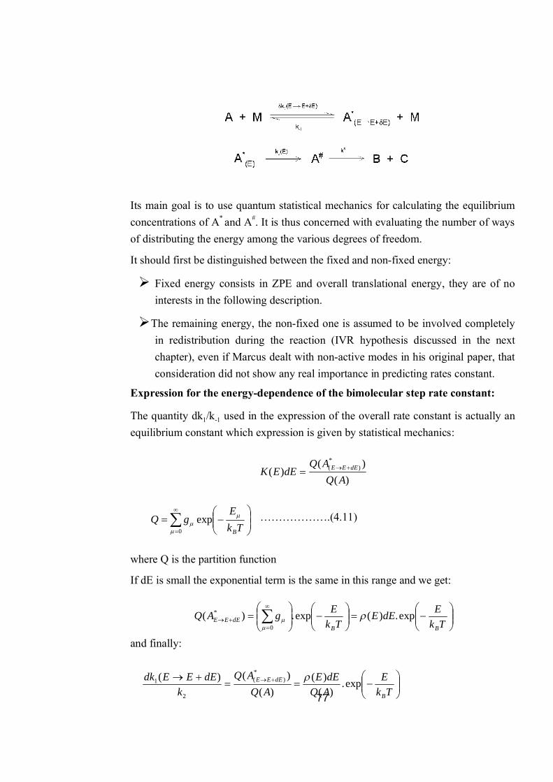
77

Its main goal is to use quantum statistical mechanics for calculating the equilibrium concentrations of A* and A#. It is thus concerned with evaluating the number of ways of distributing the energy among the various degrees of freedom.

It should first be distinguished between the fixed and non-fixed energy:

Fixed energy consists in ZPE and overall translational energy, they are of no interests in the following description.

The remaining energy, the non-fixed one is assumed to be involved completely in redistribution during the reaction (IVR hypothesis discussed in the next chapter), even if Marcus dealt with non-active modes in his original paper, that consideration did not show any real importance in predicting rates constant.

Expression for the energy-dependence of the bimolecular step rate constant:

The quantity dk1/k-1 used in the expression of the overall rate constant is actually an equilibrium constant which expression is given by statistical mechanics:

……………….(4.11)

where Q is the partition function

If dE is small the exponential term is the same in this range and we get:

and finally:

0exp

Tk

EgQ

B

)()(

)(*

)(

AQAQ

dEEK dEEE

Tk

EdEETk

EgAQBB

dEEE exp.)(exp.)(0

*

TkE

AQdEE

AQAQ

kdEEEdk

B

dEEE exp.)(

)()(

)()( *)(

2

1

78

……………….(4.12)

which is in fact the quantum Boltzmann distribution giving the thermal equilibrium proportion of molecules in the given energy range.

Expression for the energy dependence of the dissociation step:

By applying the SSA to A# of the reaction scheme:

we get: ][][

21)( *2 A

AkEk

the factor ½ coming from the fact that half of the molecules cross the extremum on the reverse direction. Then following a similar development to the TST we get the expression for the rate of dissociation:

……………….(4.13)

with x the translational energy of the molecule at the top of the barrier, m its mass, and the length of the “box”

Considering again the two species to be at thermal equilibrium, the ratio of their concentrations is then expressed as the ratio of their partition function (they have the same ground state energy). Both these species have the total energy in the same range

dEEE and the ratio of their partition function reduces to the ratio of the sum of the degeneracies, which at the energy of interest, chemical energies, can be approximated by the ratio of their density of states:

……………….(4.14)

2/1

22

mxk

)()()(

][][

*** ExNEP

AA

eq

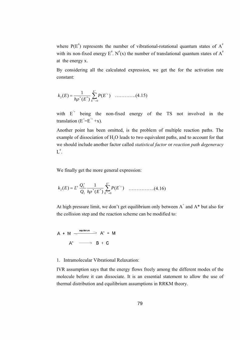
79

where P(E#) represents the number of vibrational-rotational quantum states of A# with its non-fixed energy E#. N#(x) the number of translational quantum states of A# at the energy x.

By considering all the calculated expression, we get the for the activation rate constant:

………….(4.15)

with E’+ being the non-fixed energy of the TS not involved in the translation (E+=E’+ +x).

Another point has been omitted, is the problem of multiple reaction paths. The example of dissociation of H2O leads to two equivalent paths, and to account for that we should include another factor called statistical factor or reaction path degeneracy L#.

We finally get the more general expression:

…………….(4.16)

At high pressure limit, we don’t get equilibrium only between A+ and A* but also for the collision step and the reaction scheme can be modified to:

1. Intramolecular Vibrational Relaxation:

IVR assumption says that the energy flows freely among the different modes of the molecule before it can dissociate. It is an essential statement to allow the use of thermal distribution and equilibrium assumptions in RRKM theory.

E

E

EPEh

Ek0

'**2

'

)()(

1)(

E

E

EPEhQ

QLEk0

'**

1

12

'

)()(

1)(

80

As mentioned previously, Marcus made provision for some of the degrees of freedom to be completely inactive and which could therefore not participate to the dissociation process. This energy can however be redistributed randomly between these modes and affects the density of states of the energized molecule as well as the activation rate constant.

There is little evidence that energy is rapidly redistributed between all vibrational modes involved within a time not greater than 10-11 s.

2. Strong collisions assumption

This assumption means that relatively large amounts of energy are transferred in molecular collisions (>> kT). RRKM assumes then the energization step to be single-step on contrary to ladder-climbing processes. This assumption also assumes that the molecule after collision is in a state completely independent as the one before, no dynamical details of the collision are thus necessary within that description.

A more detailed study of energization step can be done involving accurate description of the dynamics of collision, and it seems relatively important for small molecules.

3. The equilibrium hypothesis

In the thermodynamic step it was assumed as in ART that the TS is crossed as if there would be equilibrium between energized and activated molecules (SSA as if no net reaction is occurring, total equilibrium of reverse reaction).

This assumption has been proven to work well by non-statistical calculations, providing that the energy barrier is not too low. In the case where E0/kT is less than 10, it starts to be problematic, and it has been shown that when the ratio has a value of 5, approximately 8% error is introduced in the results.

4. Continuous distribution function of state density

The approximation of continuous density of states for the activated complex can be cumbersome, since most of the energy available is fixed to overcome the barrier and a part of it stored in the translational motion. This approximation holds very well for highly excited molecules (density of states becomes a continuous function of energy) but can become problematic when the energies involved are just above chemical energies.

81


a) According to RRK theory K2 increases with respect to ------------------energy.

b) Reoctants are divided from products by means of -----------state.

c) RRKM assessmes that the energization stop to be….step.

d) Equilibrssim constant is the value of Rx quotient when reaction has

reached………..

4.8 Chemical potential of perfect gas

This variant of the theory is very useful when no TS can be explicitly identified (for Morse-like potential, e.g. direct bond dissociation), where there is no saddle point (no energy barrier to overcome). It is based on the idea that there is a “bottleneck” in the phase space during the dissociation (TS is the surface which divides reactants from products and for which the phase space is the minimum). This can be explained by the fact that during the dissociation process the molecule needs to reach at a certain point, a very specific conformation without which it cannot go further to dissociate. Arrhenius equation can be written in terms of exponential of Gibbs free energy and exponential of entropy (which is the equivalent of the pre-exponential ratio of partition functions) which characterize the number of distinct states reachable with that amount of energy. Therefore when the conformation is more restrictive, the entropy is less and the pre-exponential factor is also less, leading to a smaller value for the rate constant.

To identify that state we can simply calculate the sum of states at different point of the PES and consider the point where it is the lowest (give formula of RRKM).

This is the idea of VTST. This type of calculations can be performed with the help of the software TheRate.

1. Phase Space theory:

The statistical dissociation rate constant can be calculated from the point of view of the reverse reaction. Again this procedure is limited to reaction without energy barrier (called loose TS reaction).

82

It is considering that the decomposition is governed only by the phase space available under strict energy and angular momentum conservation. Considering equilibrium between reactants and products, we get:

………………(4.17)

for which there is no need of informations on the TS.

4.9 Summary

This chapter discusses the following topics:

Basic concept of thermodynamic reactions

Spontaneous process of thermodynamics and its failures

Hinshelwood and RRK theory

RRKM theory and its approximations and some other theories

4.10 Glossary






),(),(),(

][]][[ 00

JEjEEjEEkk

ABBA

kk

AB

BAbimuni

bim

uni

83



4.1 a) T b) F c) T d) T

4.2 a) Vibrational b) Transition c) Single d) equri li qurism


1. What are unimoleculre reactions? Explain with examples. 2. Write short note on theories of unimoleculre reaction rates. 3. Give Spontaneous process for unimoleculre reaction rates. 4. What are the evidences of failures of Spontaneous process. 5. Write detailed notes on Hinshelwood and RRKM theory. 6. Discuss RRKM theory in detail.





84

Unit - 5 : Phase Equilibria Structure of unit

5.1 Objectives

5.2 Introduction

5.3 Phase Rule

5.4 Criteria for phase equilibria of multicomponent system

5.5 Phase diagrams

5.6 Solid liquid Vapour equilibrium

5.7 Solid liquid equilibria

5.8 Liquid – Vapour equilibria

5.9 Gibbs-Duhem - Margules equation

5.10 Fractional distillation of binary liquids

5.11 Solid gas equilibria

5.12 Summary

5.13 Glossory

Answer to key assessement questions


5.15 References

5.1 Objectives At the end of this unit student able is to

Understand the phase rule and the criteria for phase equilibria

Construct phase diagrams

Is study different kinds of equilibria exist between different phases

Know different variables to describe the systems

Understand the applications of phase diagrams

5.2 Introduction This unit deals with the basics of phase rule and the criteria for phase equilibria which estabilished for different systems. It gives the ideas that what kind of variables

85

to be choosen to construct the phase diagrams. It deals with the various types of equilibria possible amongst the three phases and each of the types is illustrated by taking suitable examples. The essence of steam distillation, fractional distillation is also described which may lead to very important application in purification of orgamic liquids. It deals with the basic concepts of freezing mixture, azeotrapes and the existance of various salts or phases at one atmospheric pressure and room temperature.

5.3 Phase rule A heterogenous system is one in which a number of phases coexist together in equilibrium. J. Willared Gibbs in 1876 gave the retationship between the number of phases, components and degree of freedom.

P + F = C + 2

When the different variables like temperature, composition etc. of the different phases do not undergo any change and if changed then again the same state is achieved by approach from either direction. This state is known is state of time equilibrium of phase equilibrium.

5.4 Criteria for phase equilibria of multicomponent system For a heterogeous and multieomponent system, the following equilibrium conditions must be fulfilled in order to obtain phase equilibria.

(a) Thermal equilibrium : This condition implies that the temperature of all the phases must be identical otherwise heat may flow from one phase to another. If a system consists of two phases A and B at temperature TA and TB respectively then

at equilibrium a small amount of heat dq flows from phase A to phase B then

Entropy change of phase A(dSA) = ATdq–

... (5.1)

Entropy change of phase B(dSA) = BTdq

... (5.2)

Total entropy change of the system (ds) = ATdq–

BTdq

... (5.3)

At the equilibrium ds = 0

or = ATdq

BTdq

... (5.4)

86

or TA = TB ... (5.5)

(b) Mechanical equilibrium : This condition implies that all the phases in equilibrium must be under the same pressure otherwise the matter may flow from one part to another.

If there occurs an expansion in volume dV of a phase (A) at the expense of onother phase (B), then the change in Halmhotz free energy of phase A,at equilibrium (dA) = 0

dA = dAA + dAB = –PAdV + PBdV = 0 ... (5.6)

PA = PB ... (5.7)

(c) Chemical equilibrium : This condition implies that at equilibrium, the chemical potential of any component in all the phases must be same. This is known an thermodynamic criteria for phase equilibrium of (M1)A and (M1)B are the chemical

potential of component in phases A and b respectively.

Decrease in free energy of component 1 in phase A = (M1)Adn1

Decrease in free energy of component 1 in phase B = (M1)Bdn1

If the system is closed then (G)T,P = 0

–(M1)Adn1 + (M1)Bdn1 = 0 ... (5.8)

(M1)A = (M1)B

Similarly if the system has more then three phases then

(M1)A = (M1)B = (M1)C ......... (M1)n ... (5.9)

Thus it follows that for the multicomponent system to be in equilibrium condition, the chemical potential of any component is the same in all the phases. Similarly for one component system the condition implies that the inodal free energy should be same in each phase at equilibrium.

5.5 Phase diagrams The effect of changes in variable like temperature, pressure at composition on the change of phase in a system can be easily understood when these are graphically representes. The representation of different conditons in which different phases can co-exist is known as phase diagram. When two variables like pressure and temperature are used for three component system, the variable compositions is

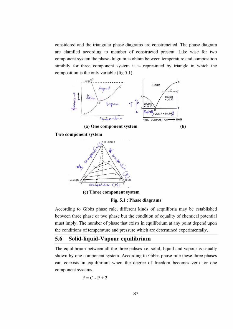
87

considered and the triangular phase diagrams are constrencited. The phase diagram are clamfied according to member of constructed present. Like wise for two component system the phase dragram is obtain between temperature and composition simibily for three component system it is represinted by triangle in which the composition is the only variable (fig 5.1)

(a) One component system (b)

Two component system

(c) Three component system

Fig. 5.1 : Phase diagrams

According to Gibbs phase rule, different kinds of aeqnilibria may be established between three phase or two phase but the condition of equality of chemical potential must imply. The number of phase that exists in equilibrium at any point depend upon the conditions of temperature and pressure which are determined experimentally.

5.6 Solid-liquid-Vapour equilibrium The equilibrium between all the three pahses i.e. solid, liquid and vapour is usually shown by one component system. According to Gibbs phase rule these three phases can coexists in equilibrium when the degree of freedom becomes zero for one component systems.

F = C - P + 2

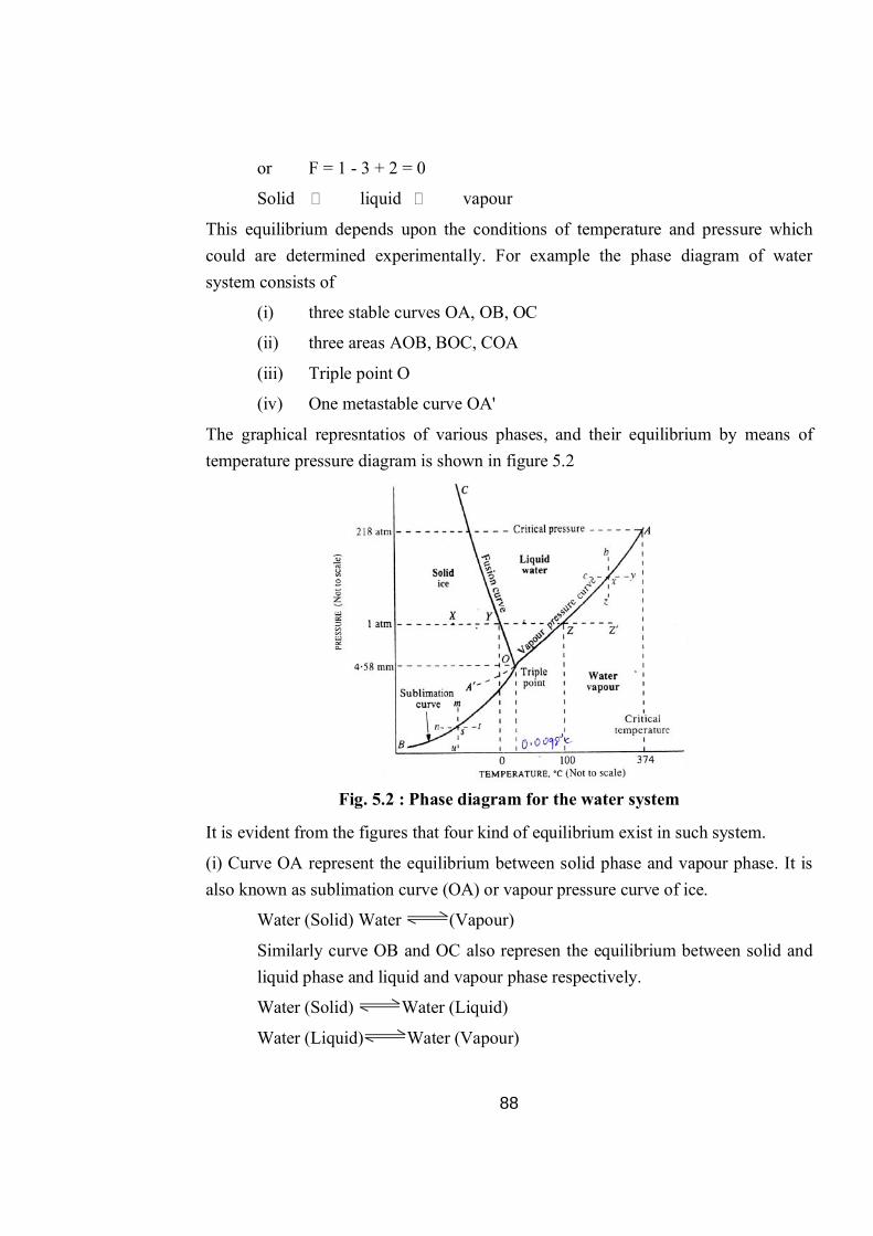
88

or F = 1 - 3 + 2 = 0

Solid liquid vapour

This equilibrium depends upon the conditions of temperature and pressure which could are determined experimentally. For example the phase diagram of water system consists of

(i) three stable curves OA, OB, OC

(ii) three areas AOB, BOC, COA

(iii) Triple point O

(iv) One metastable curve OA'

The graphical represntatios of various phases, and their equilibrium by means of temperature pressure diagram is shown in figure 5.2

Fig. 5.2 : Phase diagram for the water system

It is evident from the figures that four kind of equilibrium exist in such system.

(i) Curve OA represent the equilibrium between solid phase and vapour phase. It is also known as sublimation curve (OA) or vapour pressure curve of ice.

Water (Solid) Water (Vapour)

Similarly curve OB and OC also represen the equilibrium between solid and liquid phase and liquid and vapour phase respectively.

Water (Solid) Water (Liquid)

Water (Liquid) Water (Vapour)

89

According to Gibbs phase rule, the system becomes univariant

[ F = 1 – 2 + 2 = 1]

Curve OB is also known freezing point curve as it indicates the equilibrium at different temperature between ice and water.

Curve OC is also known as vapour pressure curve of water. Three area represent single phase. Thus behave as bivariant systems.

At the triple point O, three curves meet and an equilibrium between ice, water and

water vapour is established at 4.58 mm and 0.078°C and the system becomes non-varient.

Curve OA' represents the vapour pressure curve of supercooded water. As the conditions are slightly changed, the supercooded phase at once changes to solid ice and curve neges with OA.

Similar equilibrium between solid, liquid and vapour phase are shown by carbon dioxide system, sulphre system fig 5.3 and 5.4 etc. The triple point occurs at 5.11

atms pressure and 56.4°C temperature. CO2 gas can be solid phase at atm pressure

and by simple coling it down to –78°C without appearance of solid phases. Therefore it is commonly called as dry ice.

The phase diagram of Sulphur system represent the triple point at phase diagram of

0.025mm pressure and 120°C temperature at which the monoclinic sulphre liquid sulpher and sulphur vapour coexist in equilibrium.

Fig. 5.3 : Phase diagram for CO2 system Fig. 5.4 : Phase diagram for

sulphur system

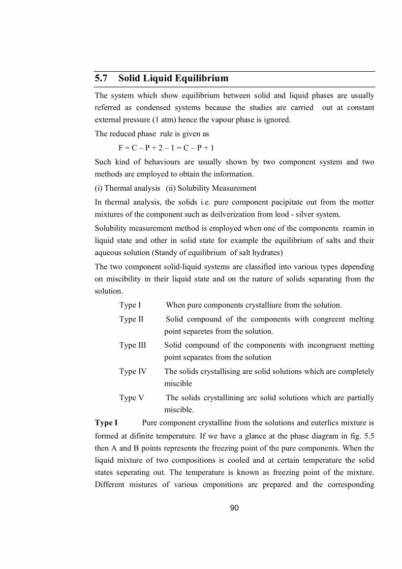
90

5.7 Solid Liquid Equilibrium The system which show equilibrium between solid and liquid phases are usually referred as condensed systems because the studies are carried out at constant external pressure (1 atm) hence the vapour phase is ignored.

The reduced phase rule is given as

F = C – P + 2 – 1 = C – P + 1

Such kind of behaviours are usually shown by two component system and two methods are employed to obtain the information.

(i) Thermal analysis (ii) Solubility Measurement

In thermal analysis, the solids i.e. pure component pacipitate out from the motter mixtures of the component such as deilverization from leod - silver system.

Solubility measurement method is employed when one of the components reamin in liquid state and other in solid state for example the equilibrium of salts and their aqueous solution (Standy of equilibrium of salt hydrates)

The two component solid-liquid systems are classified into various types depending on miscibility in their liquid state and on the nature of solids separating from the solution.

Type I When pure components crystalliure from the solution.

Type II Solid compound of the components with congreent melting point separetes from the solution.

Type III Solid compound of the components with incongruent metting point separates from the solution

Type IV The solids crystallising are solid solutions which are completely miscible

Type V The solids crystallining are solid solutions which are partially miscible.

Type I Pure component crystalline from the solutions and euterlics mixture is formed at difinite temperature. If we have a glance at the phase diagram in fig. 5.5 then A and B points represents the freezing point of the pure components. When the liquid mixture of two compositions is cooled and at certain temperature the solid states seperating out. The temperature is known as freezing point of the mixture. Different mistures of various cmponitions are prepared and the corresponding

91

freezing points and compoistions are plotted to give a phase diagram. The two curves AC and BC represnets the equilibrium between the solid and liquid phase. Along AC curve the mixture is rich in A component whilo in BC curve it is rich in B component. Thus on cooling the respective components separates out in solid phase. At point C two solids and one liquid coexist in equilibrium. This point is known as eutectic point and the correponding temperature and composition is know as eutectic temperature and eutectic composition.

Unsaturated solution

Solid B + solution

B + Eutectic

Solid A + solution

A + Eutectic

C

B

E

A

D

Fig. 5.5 : Two component system

According to Gibbs phase rule

(i) The system becomes univariant along the curves AC and BC

F = C - P + 1

F = 2 - 2 + 1 = 1

Thus either temperature or composition is sufficient to describe the systems.

(ii) The system becomes bivariant above the curve where temperature and component both are necessary to defined it. Here the solution remins unsaturated.

F = 2 - 1 + 1 = 2

(iii) The system becomes zero or variant at point C, the eutectic point as it consist of three phases two solids and one liquid mixture

F = 2 - 3 + 1 = 0

(iv) Here the component of liquid phase and the solid phase is similar areas below curves AC and BC and above DC and EC consists of liquid and the solid A or solid B and here the systems behaves as univariant system.

F = 2 - 2 + 1 = 1

Curve AC and BC are known as liquidus curves while curve AC and BC are known as solidaus curves.

Examples of such systems are :

92

Lead - Silver system

H20 - KCl system

Lead Silver System (Fig. 5.6)

The important features of lead - silver systems are following -

(i) Melting point of Silver (Ag) = 9610C

Melting point of Lead (Pb) = 3270C

Eutectic temperature of system= 3030C

Eutectic compostion of sytems = 2.6% Ag.

97.4%Pb

Liquid + Solid silver

Solid silver +

Eutectic

Liquid +

Solid lead

Solid lead

+ Eutectic

C

961

303

A

303 c

BLiquid melta

b

327

2.6% Ag100% Pb 100% Ag

TEM

PER

ATU

RE (°

C)

COMPOSITION Fig. 5.6 : Phase diagram for lead – silver system

Significance of Lead - Silver- System

Galena, the ore of lead pbs is usually associatede with lead. Since silver is soluble in lead, so some extent of it passes to the lead during its extraction process. Lead is now known as argentiferous lead. To separate lead from the mixture, it is cooled till the lead is separated out and the mixture now becomes rich in silver. The process continues till the entectic point is reached where an alloy containing 2.6% Ag is obtained. This process is known as pettinsons process. Type II The systems in which pure component under suitable conditinos of temperature and composition, forms compound which is stable upto its melting point and melts to give a liquid of same composition. This point is known as congruent melting point of the compound.

For example Mg - Zn system, Fe2Cl6-H20 system etc. (fig 5.7)

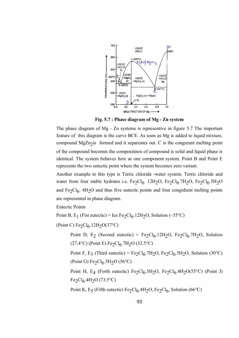
93

Fig. 5.7 : Phase diagram of Mg - Zn system

The phase diagram of Mg - Zn systems is representive in figure 5.7 The important feature of this diagram is the curve BCE. As soon as Mg is added to liquid mixture, compound MgZn2is formed and it separeates out. C is the congreunt melting point

of the compound becomes the compositinos of compound is solid and liquid phase is identical. The system behaves here as one component system. Point B and Point E represents the two entectic point where the system becomes zero variant.

Another example to this type is Terric chloride -water system. Terric chloride and water from four stable hydrates i.e. Fe2Cl6. 12H2O, Fe2Cl6.7H2O, Fe2Cl6.5H2O

and Fe2Cl6. 4H2O and thus five eutectic points and four congrdient melting points

are represented in phase diagram.

Eutectic Points

Point B, E1 (Fist eutectic) = Ice Fe2Cl6.12H2O, Solution (–55°C)

(Point C) Fe2Cl6.12H2O(37°C)

Point D, E2 (Second eutectic) = Fe2Cl6.12H2O, Fe2Cl6.7H2O, Solution

(27.4°C) (Point E) Fe2Cl6.7H2O (32.5°C)

Point F, E3 (Third eutectic) = Fe2Cl6.7H2O, Fe2Cl6.5H2O, Solution (30°C)

(Point G) Fe2Cl6.5H2O (56°C)

Point H, E4 (Forth eutectic) Fe2Cl6.5H2O, Fe2Cl6.4H2O(55°C) (Point J)

Fe2Cl6.4H2O (73.5°C)

Point K, E5 (Fifth eutectic) Fe2Cl6.4H2O, Fe2Cl6, Solution (66°C)

94

Fig. 5.8 : Phase diagram of FeCl3 — H2O system

Type III Binary system in which the two component are completely miscible in liquid phase and produce a compound which is not stable up to its melting point. Thus when it is observed to melt, it produces a liquid phase with different compostion and a new solid phase. This point is known as incongruent melting point.

S S1 + Liquid

Example of such syste

NaCl – H2O system

Na2SO4 – H2O system

NaCl and H2O react to form NaCl 2H2O which has incongruent melting point

0.150C. When NaCl is added in solution, the eutectic point is observed at -210C. Where NaCl 2H2O, ice and solution are in equilibrium. This point is known as

cryohydric point. Thus ice and salt mixture has wide applications in domestic a well as commercial area as it reaches to very low temperature and hence can be used as freezing mixtures.

Ice with NaNO3 may lead to -180C temperature similarly mixture of alcohal and

solid CO2 results very low temperature i.e. 720C.

There are three component systems also which shown solid-liquid equilibrium. For example a system of two salts and water (fig. 5.9) when two salts shown some solubility and also form saturated solution.

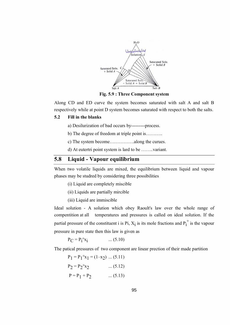
95

Fig. 5.9 : Three Component system

Along CD and ED curve the system becomes saturated with salt A and salt B respectively while at point D system becomes saturated with respect to both the salts. 5.2 Fill in the blanks

a) Desilurization of bad occurs by---------process.

b) The degree of freedom at triple point is………..

c) The system become…………….along the curues.

d) At eutertri point system is lard to be ……..variant.

5.8 Liquid - Vapour equilibrium When two volatile liquids are mixed, the equilibrium between liquid and vapour phases may be studred by considering three possibilities

(i) Liquid are completely miscible

(ii) Liquids are partially mircible

(iii) Liquid are immiscible

Ideal solution - A solution which obey Raoult's law over the whole range of compentition at all temperatures and pressures is called on ideal solution. If the

partial pressure of the constituent i is Pi, Xi is its mole fractions and Pi° is the vapour

pressure in pure state then this law is given as

PC = Pi°xi ... (5.10)

The patical pressures of two component are linear prection of their made partition

P1 = P1°x1 = (1–x2) ... (5.11)

P2 = P2°x2 ... (5.12)

P = P1 + P2 ... (5.13)

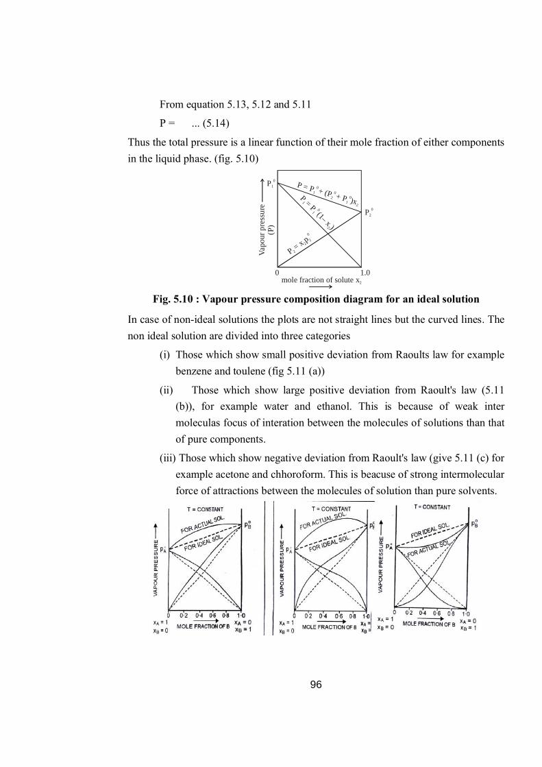
96

From equation 5.13, 5.12 and 5.11

P = ... (5.14)

Thus the total pressure is a linear function of their mole fraction of either components in the liquid phase. (fig. 5.10)

P10

P20

0 1.0mole fraction of solute x2

P = P +10

(P + P )x 2

12

0 0P =1

P(1– x )

1

2

0

P =2

x p 2

20

Vapo

ur p

ress

ure

(P)

Fig. 5.10 : Vapour pressure composition diagram for an ideal solution

In case of non-ideal solutions the plots are not straight lines but the curved lines. The non ideal solution are divided into three categories

(i) Those which show small positive deviation from Raoults law for example benzene and toulene (fig 5.11 (a))

(ii) Those which show large positive deviation from Raoult's law (5.11 (b)), for example water and ethanol. This is because of weak inter moleculas focus of interation between the molecules of solutions than that of pure components.

(iii) Those which show negative deviation from Raoult's law (give 5.11 (c) for example acetone and chhoroform. This is beacuse of strong intermolecular force of attractions between the molecules of solution than pure solvents.

97

fig 5.11 Vapour pressure - composition curves for non ideal solution showing deviations from ideal behaviour.

Vapour pressure – Compsition and Boiling point – Composition curves of completely miscible binary solutions.

If we take binary mixture of two liquid components A and B which are completely miscible with each other and on the basis of nature of vapour pressure composition curves they are divided into three categories –

fig 5.12 Vapour pressure composition curve of completely miscible

liquids.

Type I mixture : Figure (5.12 (a)) shows the variation of vapour pressure with composition of the mixture.

figure 5.13 (a) shows that boiling point of the mixtures of A and B lie in between boiling of point of pure A and pure B. It do not show any maximum of minimum.

Type II mixture : In figure 5.12 (b) it is evident that vapour pressure curve shows a maximum at C point and the boiling point will be the lowest at C point corresponding to this composition shown in fig. 5.13 (b)

Type III mixture : The vapour pressure curve [fig 5.12 (e)] shows a minimum at C point and the corresponding boiling point will be at the highest temperature (at C point). The liquid mixture corresponding to point having low or minimum boiling points are called azeotropes.

5.9 Gibbs - Duhem Margules equations Liquid and Vapour composition in equilibrium may be stnderd by Gibbs - Duhem- Margules equations.

If nA and nB are the number of moles of components A and B respectively then

according to Gibbs Duhem equation.

nAdMA + nBdMB = 0

98

Here MA and MB are the respective chemical potential

or xAdMA + xBdMB = 0

xAand xB are the molar practions of components A and B respectively.

The chemical potential of any component of a liquid mixture is given as

Mi = Mi + RTlnfi

where fl is the fugacity in liquid or vapour phase in equilibrium. On differentiating

above equation

dMdmi= RTdlnfi

Or xARTdlnfA + xBRTdlnfB = 0

Or B

A

Xlndflnd

= B

B

Xlndflnd

If the vapour behaves ideally then the fugacity may be replaced by vapour pressure

dlnPA/dlnxA = dlnPB/dlnxB

This equation is known as Gibbs - Duhem- Margules equation.

This gives the relationship between the composition of the mixture in the liquid phase with the paitial vapour pressure in the gase phase.

5.10 Fractional Distillation of Binary Liquid Solutions The boiling point - composition curves of solution may be useful in understanding the distillation process of three types.

1. Type I [fig 5.13 (a)] Let the solution of composition corresponding to x point is 1. heated. It will start boiling at T temperature. At this point the vapour will have the composition X1. Since X1 would be richer in B than X while X will

be richer in A than X1. If we consider another point y then it will require high

temperature (T1) to boil. The corresponding vapour will again be richer in B.

99

Fig. 5.13(a) : Boiling temperature – composition curves for liquid and vapour

phases of binary solution of Type 1.

Thus if the process is continued, the liquid will become richer in A and finally only liquid A will remain in liquid phase and vice verva. Thus it is possible to state both the pure constituents from each other. By means o fractionating colums this can be achieved such kind of distillation is known as feactional distillation.

Solution of Type II

The BP compention curve meet at the minimum point C where the liquid mixture distil over without change of compossntion. This mixture is known as constant boiling mixtures or azeotropic mixture. Such cases only on pure component (either A or B) and final at distillate of composition C is obtained on fractional distillation.

Fig. 5.13 (b) : Boiling temperature – composition curves for liquid and

vapour phases of binary solutions of Type II.

Type III In such type of cases the mixture having the maximum boiling point is obtained. On froctional dislillation a distillate of pure component (either A and B) and reduce of constant boiling mixture is obtained.

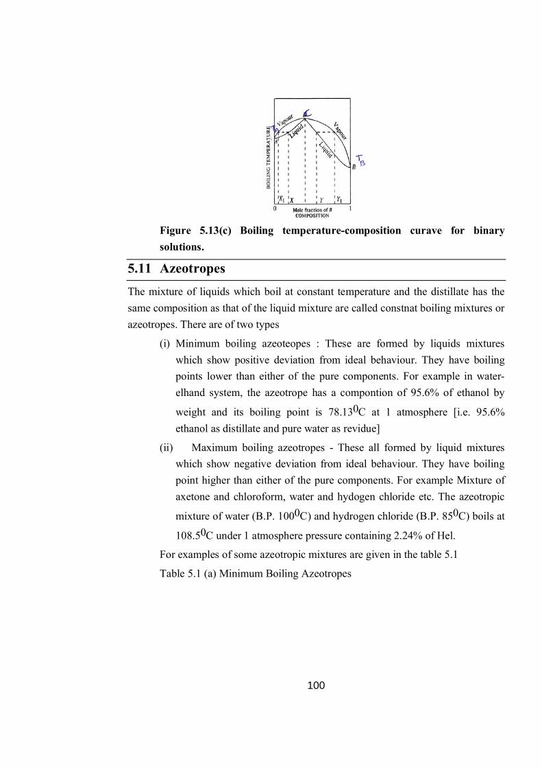
100

Figure 5.13(c) Boiling temperature-composition curave for binary

solutions.

5.11 Azeotropes The mixture of liquids which boil at constant temperature and the distillate has the same composition as that of the liquid mixture are called constnat boiling mixtures or azeotropes. There are of two types

(i) Minimum boiling azeoteopes : These are formed by liquids mixtures which show positive deviation from ideal behaviour. They have boiling points lower than either of the pure components. For example in water-elhand system, the azeotrope has a compontion of 95.6% of ethanol by

weight and its boiling point is 78.130C at 1 atmosphere [i.e. 95.6% ethanol as distillate and pure water as revidue]

(ii) Maximum boiling azeotropes - These all formed by liquid mixtures which show negative deviation from ideal behaviour. They have boiling point higher than either of the pure components. For example Mixture of axetone and chloroform, water and hydogen chloride etc. The azeotropic

mixture of water (B.P. 1000C) and hydrogen chloride (B.P. 850C) boils at

108.50C under 1 atmosphere pressure containing 2.24% of Hel.

For examples of some azeotropic mixtures are given in the table 5.1

Table 5.1 (a) Minimum Boiling Azeotropes

101

A B A B Boiling Point % composition of B

H2O C2H5OH 100°C 78°C 78.15°C 95.6%

CHCl3 C2H5OH 61°C 78°C 59.3°C 6.8%

CH3COCH3 CS2 56.25°C 46.25°C 39.25°C 67%

Compnents Boiling point Azeotrope

(b) Maximum Boiling Azeotropes

A B A B Boiling Point % composition of B

H2O HCl 100°C –85° 108.5°C 20.24%

H2O HNO3 100°C .86°C 120.5°C 68%

Compnents Boiling point Azeotrope

5.12 Immiscible Liquids Immiscible liquids are those which do not disolve in each other. In fact the addition of one liquid to other does not alter the properties of either liquid. Each component of the liquid mixture exeits its own vapour pressure independent of the presence of other. Thus the total vapour pressure of the mixture of two immiscible liquides in any propertion will be the sum of the vapour pressure of the pure liquids at that temperature.

If AP and

BP are the vapour pressures of pure liquids A and B respectively the total vapour pressure (P) will be given as

P = AP +

BP

Since the liquid boils at one atmosphere pressure (i.e. its vapour pressure becomes equal to atmosphereic pressure which is usually 1 atm)

Therefore, it is evident from the above equation that any mixture of two immiscible liquids will boil at a lower temperature than either of the two liquids alone (i.e. pure component) Since the total vapour pressure is constnat and is independent of the amounts of the liquids present. So the boiling point of the mixture will remain constant as long as the two liquids are present together. As soon as one of the liquids has completely boiled away, the temperature. suddenly rises to value equivalent to the boiling point of remaining liquid.

If nA and nB are the number of moles of component A and B respectively in vapour

phase at the boiling point then

102

B

A

PP

= B

A

nn

= BB

AA

M/WM/W

= AB

BA

MWMW

or = B

A

WW

= B

A

B

A

MM.

PP

Here WA and WB are actual masses of respective components in distillate and MA

and MB are their respective molar masses. Thus the masses of the liquids in the

distillate will the ratio of their partial pressures and molar masses. Steam Distillation :Steam distillation is a method to purify organic liquids having high boiling points. An organic liquid immisible with water and with relatively high boiling point can be distilled at a much lower temperature. The apparatns is shown in figure 5.14. The steam generated is passed in liquid and then the vapour of the liquid mixed with steam pass over and condersed in the recived. The process can be understood by means of following example.

Fig. 5.14 : Exerimental set-up for steam distillation.

A mixture of water and chlorobenzene at 740mm pressure has been bound to boil at

900C (B.P. of pure chlorobenzene = 1320C at 760 mm pressure). The vapour

pressure of pure water mm1.530P0OH2 and chlorobenzene mm210P0

ClHC 56 naek the total

vapour pressure 740.1mm. The mixture is made to boil by passing steam through it. The vapours are condensed in the receiver. The vapours and the distillate have the composition.

OH

ClHC

2

56

WW

=

OHOH

ClHCClHC

22

5656

P.MP.M

= 2.1801.2305.112210

= 147.2

103

This means that the distillate will contain about 70% chlorobenzene and remaining water. Higher boiling liquid can be purified at a much lower temperature by steam distillatino to avoid their decomposition.

5.13 Partially Miscible Liquids There are some liquids which dissolve partially in each other. Four types of partially miscible liquid systems are found.

1. Type I - Those liquids mixtures in which the partial miscibility increases on increaring the temperature. for example (i) phenol -water system (ii) anitine water system (iii) anilive heance system etc.

2. Type II - Those in which the partial miscibility increases on lowering the temperatures. For example (i) diethylamine -water system (ii) triethyl amine - water system.

3. Type III - Those in which the partial misibility increases either with increasing or decreasing the temperature at certain ranges. for example (i) water - micoline (ii) water- p- picoline system.

4. Type IV - Those in which complete miscible temperature cannot be obtained. For example (i) ether - water system (ii) chloroform - water system

Critical solution temperature or consolute temperature

When two partially miscible liquids are mixed together, two phases having different composition in equilibrium with each other at a given temperature are formed. Those are known as conjugate phases. The temprature at which two partially miscible liquids become completely miscible is known as consulate temperature or critical solution temperature (CST). Some liquid paiss attain complete miscibility above CST then it is known to have upper critical solution temperature, while some attain complete miscibility below CST then it is known to have lower critical solution temperature. Some of the mixtures show upper as well as lower consolute temperature. Effect of impurities on CST

1. Due to the presence of impurity the mutual solubility of liquids may decrease and hence the CST increases. This is because of solubility of impurity in either one of the two liquids. For example Addition of KCl to phenol water system.

104

2. If the impurity is soluble in both the liquides then it increase the mutual solubility of liquids with each other hence the CST decrease. For example Addition of succinic acid + phenol water system.

Phenol -water system - When phenol and water are mixed together, a pair of solutions with different compositions are formed. As the temperature is raised, the mutual solubility of each other increases and at particulars temperature, the composition of two conjugate phases becomes similar and the system becomes homogenous. If the variation of mutual solubility with compostion is plated then

paraliolie curve is obtained. The upper CST has been found to 660C and the [fig 5.15 (a)] compositions is 34% phenol by weight. If we take the point X lying on the left hand side to parabolic curve. It correspoinds to other point y on the right hand side of the curve and the line xy is known as tie-line Any point lying outside the curve on LHS or RHS represent the unsaturated solution and above c the system will have one homogenous solution. Triethyl - water system - It is endent from figure 5.15 (b) that the mutual solibility of liquid do increase with decrease in temperature and thus has the lower critical solution temperature (18.5°C) Nicoltine -water system - This system shows both the upper critical solute on temperature as well as the lower critical solution temperature i.e. the mutual solubility increase as well as decrease with the rise or fall in temperature. The upper CST as 208°C and the lower CST is 60.8°C. The system remains partially miscible between these two temperature. (fig 5.15 )

(c)) Fig. 5.15(a) : Phenol-water sysem Fig. 5.15(b) : Triethylamine-water

system

105

Fig. 5.15 (c) : Nicotine-water system

5.11 Solid - Gas Equilibria

Binary systems in which solid and gas phase consist in equilibrium have significance only when the components form one or more compounds in the solid phase. For example CuSO4 and water.

The salt hydrate system of CuSO4 and H2O under different conditions from four

solid phases namely.

(i) CuSO4 . 5H2O (ii) CuSO4 . 3H2O (iii)CuSO4.H2O (iv) CuSO4 (anhydrous)

Since CuSO4 . 5H2O is gradnerlly hydrated, so its dissociation can be represented in

the following manner

CuSO4 . 5H2O(S) CuSO4 . 3H2O(S) + 2H2O (g)

CuSO4 . 3H2O(S) CuSO4 . 3H2O(S) + 2H2O (g)

CuSO4 . H2O(S) CuSO4(S) + H2O (g)

At each stage two solids and one gaseous phase are in equilibrium, thus the degree of freedom will be unity. Thus if temperature is keept constant the vapour pressure of water also remain constant

F = C – P + Z = 2 – 3 + 2 = 1

When CuSO4 . 5H2O crystals are connected to a vaccum pump, the pressure of

water vapour can be measured. At A point the vapour pressure is 45.4mm, CuSO4

5H2O changes into CuSO4 . 3H2O along AB live and after the complete reaction the

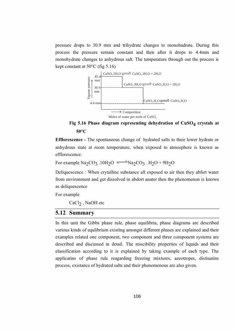
106

pressure drops to 30.9 mm and trihydrate changes to monohudrate. During this process the pressure remain constant and then after it drops to 4.4mm and monohydrate changes to anhydrous salt. The temperature through out the process is kept constant at 50°C (fig 5.16)

CompositionMoles of water per mole of CuSO4

4.4 mm

30.9 mm

45.4 mm

CuSO .5H O 4 2 CuSO .3H O + 2H O4 2 2

Vapo

ue p

ress

ure

CuSO .3H O 4 2 CuSO .H O + 2H O4 2 2

CuSO .H O 4 2 CuSO .H O 4 2

Fig 5.16 Phase diagram representing dehydration of CuSO4 crystals at

50°C

Efflorescence - The spontaneous change of hydrated salts to their lower hydrate or anhydrous state at room temperature, when exposed to atmosphere is known as efflorescence.

For example Na2CO3 .10H2O Na2CO3 . H2O + 9H2O

Deliquescence : When crytalline substance all exposed to air then they abfsrt water from environment and get dissolved in abdort anater then the phenomenon is known as deliquescence

For example

CaCl2 , NaOH etc

5.12 Summary In this unit the Gibbs phase rule, phase equilibria, phase diagrams are described various kinds of equlibrium existing amongst different phases are explained and their examples related one component, two component and three component systems are described and discussed in detail. The miscibility properties of liquids and their elassification according to it is explained by taking example of each type. The applicatins of phase rule reagarding freezing mixtures, azeotropes, distiuatins process, existance of hydrated salts and their phenomenous are also given.

107

5.12 Glossary

Phase : Physically distinct, chemically enert and mechanically separable part

of system.

Component : An element or a compound present in a system.

Sulabimation ceerue: Curve where social is in equilibission

Triple point : where all the three phases coexssst

Entectre point : Lowest temperature at which the liquid motal can exist.

Critical solution temperate : Temperature at which two partially miscible

liguid become

Answer to key assessment questions 5.1 a) T b) F c) T d) T

5.2 a) Pettiners b) zero c) univeriant d) hon

5.3 a) miscible b) two c) high d) azrotropes

5.13 Review Questions 1. Define Gibbs phase rule.

2. Discuss the criteria of phase equilibirum for multicomponent system.

3. Draw the phase diagram of water system. What is difference between ice and dry ice?

4. Draw and discuss the phase diagram of Lead-Silver system and also describe the Pattinsons process for enrichment of silver.

5. What do you understand by congruent and incongruent melting point. Give an example of each.

6. Draw the phase diagram of Mg-Zn system and discuss its salient features.

7. What are ideal and non ideal solution ?

8. What do you understand by fractional distillation? Discuss it on the basis of boiling temperature - compostion curves.

108

9. What are azeotropes? Discuss the system of having minimum boiling azeotrops.

10. Write short note on steam distillation.

11. What are partially miscible liquids? Discuss critical solution temperature and the effect of impurity on it.

12. Discuss phenol - water system.

13. Describe Gibbs Duhen Margules equation.

5.14 Refrences

1. Physical Chemistry by Bourdan

2. Physical Chemistry by S. Glasston

3. Physical Chemistry by Puri and Sharma

4. Phase Rule by Y.K. Gupta

109

Unit – 6 : Physical Transformation of Simple Mixtures

Structure of Unit

6.1 Objectives

6.2 Introduction

6.3 Partial molar properties

6.4 Partial molar volume

6.5 Partial molar Gibbs free energy

6.6 Thermo dynamics of functions of mixing

6.7 Colligative properties

6.8 Elevation of boiling point

6.9 Depression in freezing point

6.10 Solubility behavious of ideal solution

6.11 Osmesis

6.12 Summary

6.13 Glossory



6.15 References and suggested reading

6.1 Objectives

While reading this unit the learner will be able to

Understand the concept of partial molar properties and their variation with temperature and pressure.

Derive the expression for various colligatiure properties ther modynamically.

Understand the thermodynamic mixing of functions.

Compharize the applications of different properties with reference to chemical as well as biological systems.

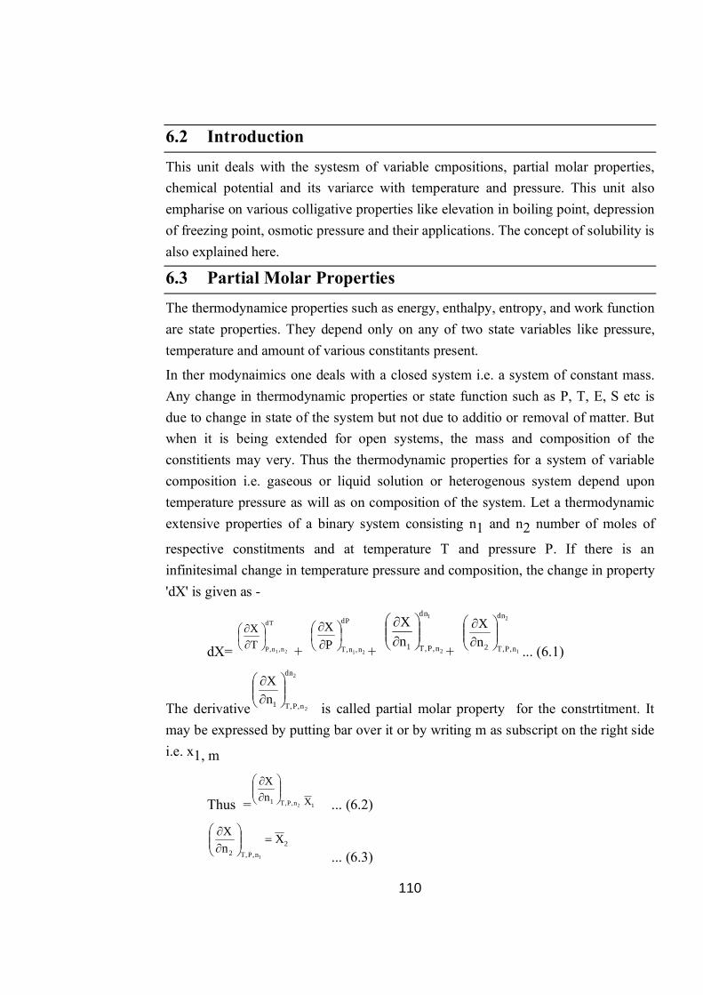
110

6.2 Introduction This unit deals with the systesm of variable cmpositions, partial molar properties, chemical potential and its variarce with temperature and pressure. This unit also empharise on various colligative properties like elevation in boiling point, depression of freezing point, osmotic pressure and their applications. The concept of solubility is also explained here.

6.3 Partial Molar Properties The thermodynamice properties such as energy, enthalpy, entropy, and work function are state properties. They depend only on any of two state variables like pressure, temperature and amount of various constitants present.

In ther modynaimics one deals with a closed system i.e. a system of constant mass. Any change in thermodynamic properties or state function such as P, T, E, S etc is due to change in state of the system but not due to additio or removal of matter. But when it is being extended for open systems, the mass and composition of the constitients may very. Thus the thermodynamic properties for a system of variable composition i.e. gaseous or liquid solution or heterogenous system depend upon temperature pressure as will as on composition of the system. Let a thermodynamic extensive properties of a binary system consisting n1 and n2 number of moles of

respective constitments and at temperature T and pressure P. If there is an infinitesimal change in temperature pressure and composition, the change in property 'dX' is given as -

dX=

dT

n,n,P 21TX

+

dP

n,n,T 21PX

+

1

2

dn

n,P,T1nX

+

2

1

dn

n,P,T2nX

... (6.1)

The derivative

2

2

dn

n,P,T1nX

is called partial molar property for the constrtitment. It may be expressed by putting bar over it or by writing m as subscript on the right side i.e. x1, m

Thus = 2n,P,T1nX

1X ... (6.2)

2

n,P,T2

XnX

1

... (6.3)

111

From equation (6.2) and (6.3), equation (6.4) may be rewritten as

dX =

dT

n,n,P 21TX

+

dP

n,n,T 21PX

+ 11dnX + 22dnX ... (6.4)

At constant temperature (dt = 0) and consitant pressure (dp=0) equation (6.4) reduce to

dXT, P = 11dnX + 22dnX + ... (6.5)

If the system at constant T and P be enlarged in such a manner that the mole fraction of each component remains constant i.e. n1 and n2 are though changed x1 and x2 are

unchanged. The molar fraction of component 1 = x1 = nn1

and the mole fraction of

component 2 = x2 =

n1 = x1n, n2 = x2n

Here n = n1 + n2

If there is small change in number of moles i.e.

dn1 = x1dn, dn2 = x2dn ... (6.6)

By introductin these terms from equation (6.6) in respective partial molar properly is equal to the total property of the system of a given composition at constant temperature and pressure. This is called additional rule.

On integrating equation (7.5) we get

XT, P, n = 2211 XnXn ... (6.7)

Now for a null component system at given temperature T and pressure P

XT, P, n = + 332211 XnXnXn ........ , in X ... (6.7)

iiXnX iiXnX ... (6.7)

The sum of the products of mole of each component and defferentiating equation 6.8 at constnan temperature and pressure

(dX)TP= 11 Xdn + 11dnX + 22 Xdn + 22dnX + ii Xdn .... + iidnX ... (6.2)

From equation (6.5) and equation (6.10)

11 Xan 11 Xan + 22 Xan + ii Xan ......... = 0 .... (6.12)

112

or = ii Xdn 0 .... (6.12)

(6.11) or (6.12) is known as Gibbs Duhem equation. It suggests that the partial molar quantities cannot change independently of one another.

Partial molar quantity or any component is defined as the rate of change of proeperty with the change in the amount of the component when the temperature, pressure and the amount of other components of the system are constant. Thus is an intensive property and not an extensive one. Its value does not depend on the amount of the substance but only on the composition which is the ratio of n's to one another at the give temperature and pressure.

The other partial molar quantities are shown in table 6.1

Partial molar property Symbol Defining equation

Partial molar volume iV in,P,TinV

Partial molar energy iE in,P,TinE

Partial molar enthalpy iH in,P,TinH

Partial molar entropy iS in,P,TinS

Partial molar free energy iG in,P,TinG

Partial molar work function iA in,P,TinA

The Gibbs Duhem equation for various partial molar properties are given as

0EdnEdn 2211

0HdnHdn 2211

0AdnAdn 2211

0SdnSdn 2211

113

6.4 Partial Molar Volume For a binary system if nA and nB are the number of moles of constituents A and B

respectively, then the change in partial molar volume at temperature T and pressure P is given as.

dVT, P = BBAA dnVdnV ... (6.13)

From equation no (6.8)

V = BBAA VnVn ... (6.14)

On differentiating and equating the equation with (6.13)

0VdnVdn BBAA ... (6.15)

Equation (6.15) is another example of Gibbs Duhem equation.

6.5 Chemical Potential (Partial molar Gibbs free energy) If the Gibbs energy for a mulltcomponent system is represented by G then it is given as.

G = f (T, P, n1, n2) ... (6.16)

Here n1 and n2 are the number of molers of two constitments 1 and 2 respectively.

Thus the change in Gibbs free energy is given as

dT

TGdG

21 n,n,P

+

dPPG

21 n,n,T

+ 1

n,P,T1

dnnG

2

+ 2

n,P,T2

dnnG

1

... (6.17)

Or dT

TGdG

21 n,n,P

+

dPPG

21 n,n,T

+ 11dnG + 22dnG ... (6.18)

Or dT

TGdG

21 n,n,P

+

dPPG

21 n,n,T

+ M1dn1 + M2dn2 ... (6.19)

Here ,

The partial molar free energy is known as chemical potential and is represented by a specific symbol which is equal to the change in Gibbs free energy with the change in mole of component when the temperature, pressure and mole of other components are kept constant.

The chemical potential is an intensive property of the system. For a closed system dn1=0, dn2 =0 thus from equation (6.20)

114

dP

PGdT

TGdG

ii

in,Tn,P

n

... (6.20)

Since for a closed system

dG = –SdT + VdP ... (6.21)

Comparing equation (6.20) and (6.21) we get

i

n,P

S–TG

C

. .. (6.22)

ii n,P,Tn,Pi T

Gn

... (6.23)

From equation (6.19), (6.22) and (6.23)

dG = –SdT + VdP + M1dn1 + M2dn2 ...(6.24)

At constant temperature (dT=0) and constant pressure (dP = 0), equation (6.24) becomes

dG = M1dn1 + M2dn2 ...(6.25)

On integeating equation (6.25), we get

G = n1M1 + n2M2 ...(6.26)

Differstiating equation (6.26) following equation may be obtained

dG = M1dn1 + M2dn2 + n1dM1 + n2dM2 ..(6.27)

Equating equation (6.28) and (6.29)

–SdT + VdP + SMidni = SMidni + SnidMi

–SdT + VdP – SnidMi = 0 ... (6.28)

If dT=0 and dP =0 then equation (6.28) reduces to

SnidMi = 0

for a binary system

n1dM1 + n2dM2 = 0

dM1 = – 2

1

2 dMnn

= ... (6.29)

Here x1 and x2are mole fractions of the respective combitnents equation (6.31) is

another form of Gibbs Duhem equation.

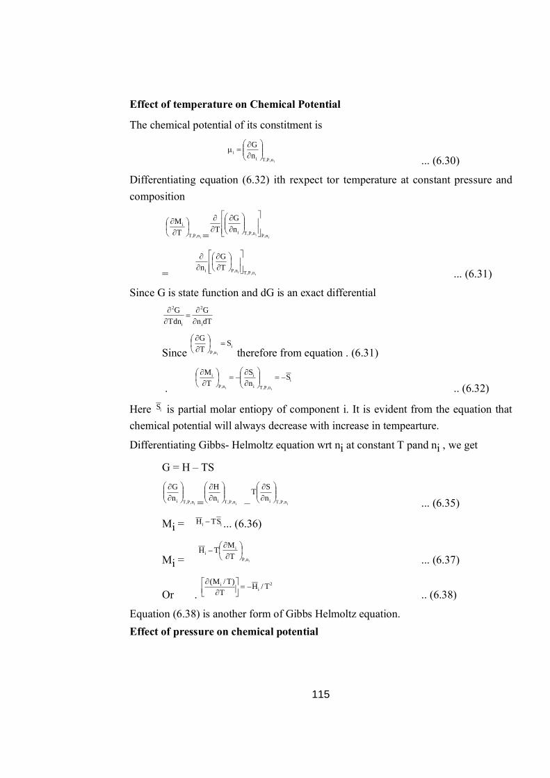
115

Effect of temperature on Chemical Potential

The chemical potential of its constitment is

in,P,Tii n

G

... (6.30)

Differentiating equation (6.32) ith rexpect tor temperature at constant pressure and composition

in,P,T

i

TM

= ii n,Pn,P,TinG

T

= ii n,P,Tn,Pi T

Gn

... (6.31)

Since G is state function and dG is an exact differential

dTnG

TdnG

i

2

i

2

Since i

n,P

STG

i

therefore from equation . (6.31)

. i

n,P,Ti

i

n,P

i S–nS–

TM

ii

.. (6.32)

Here iS is partial molar entiopy of component i. It is evident from the equation that chemical potential will always decrease with increase in tempearture.

Differentiating Gibbs- Helmoltz equation wrt ni at constant T pand ni , we get

G = H – TS

in,P,TinG

= in,P,TinH

– in,P,TinST

... (6.35)

Mi = ii ST–H ... (6.36)

Mi = in,P

ii T

MT–H

... (6.37)

Or . 2

ii T/H–T

)T/M(

.. (6.38)

Equation (6.38) is another form of Gibbs Helmoltz equation. Effect of pressure on chemical potential

116

Differentiating in,P,Tii n

GM

wrt to pressure at constant temperature of at conetant

molar of constituents

iii n,P,Tn,P,Tin,T

i

nG

PPM

ii n,P,Tn,Ti PG

n

... (6.39)

Since G is a state function, dG is an exact differential and thus

PnG

PdnG

i

2

i

2

ii n,P,Tn,Ti P

Gn

... (6.40)

Here iV is the partial molar volume of i th constitment. 6.1 Complete the following a) b) Partial molar volume can be given as---------- c) for Closed system dg = tvdp d) Chemical potentate will always ---------------------------with increase in temperature. 6.2 Choose the correct alternative a) Nodal freezing point constant is also called as ………………….(calligature property/Crysocopic constent) b) Tj decreases, as the mole protion of solute (increased dereased) c) B lullometrere constant is mdal (F.B./B.P.) d) Free energy of mixing is always ………………(negative/positive)

6.6 Thermodynamic Function of Mixing When two or more substance are mixed in a system, the measurable properties undergo change and the extent of change is different for different systems. The thermodynamic function of mixing is the property of the mixture if the total property of pure components is not considered.

Gibbs free energy of mixing (DGmix)

117

A vessel containing theree compornents fitted with partitions that can be removed is considered. Each compartment is filled with know amounts (n1,n2 and n3) of

different pure gases at the same temperature and pressure (fig 6.1)

n1 n2 n3

three compartments

Removable partitions Initia lstate

(n + 1 n + n )moles 2 3

Final state

Fig 6.1 Mixing of three pure gases at constant temperature and consistant

pressure.

As the partitions separrating the gases are pulled out the final state is achieved as shown in the figure.

The free energy of gases before mixing is given as

Ginitial = n1m10 + n2m20 + n3m30 = nimi0 ... (6.41)

Here m10 is the chemical potential of pure gas.

The total free energy after mixing

Gfinal = n1m1 + n2m2+ n3m3= nimi ... (6.42)

mi is the chemical potential of pure gas in the mixture.

The free energy of mixing (DGmix)) is given as

DGmix = Gfinal – Ginitial

= nimi – nimi0 ... (6.43)

If there gases are assumed to be ideal then

ni = mi0+ RT lnxi ...(6.44)

Substituting the value of the mi from equation (6.44) in equation (6.43)

DGmix = n1m10 + RT nilnxi – nimi0

DGmix = RT nilnxi ... (6.45)

Thus the free, energy change at constant T and P can be calculated using equation (6.45)

118

When two three ideal gases are mixed at constant temperature and pressure, . G mix is given as

DGmix = RT(n1lnx1 + n2lnx2) ... (6.46)

DGmix = RT(n1lnx1 + n2lnx2 + n3lnx3) ... (6.47)

If n is the total number of moles than dividing equation (6.46) by n, we get

=

2

21

1 xlnnnxln

nnRT

= RT(x1lnx1 + x2lnx2)

Here x1 and x2 are the mole fraction of the two constituments respectively

= RT xilnxi ... (6.48)

Equation (6.48) is valid for ideal solutions also.

Since the mole fraction is always less than one so lnxi would always be negative.

Thus free energy of mixing is alway negative. Since mixing is spontameous, hence spontaneous mixing is always accompanied with decrease in Gibbs free energy.

6.7 Colligative Properties A Colligative properpty is the property which depends only on the number of particles of the solnte in the solution and not no the nature of particular particle. The word colligative is derived by the latin word colliare which means to bind together. The Colligative property is used particularly with reference to dilute solution. For example, the addition of a non-volalite solute to the solvent causes a lowering in vapour pressure of the solvent and hence comes an increase in boiling point. Expression in freezing point and or molar pressure are also examples of colligative properties which are also influenced by the previous one.

6.8 Elevation of boiling point Boiling point of a liquid is the temperature at which its vapour pressure becomes equal to the atmospheric pressure. If a non-volalile solmte is added to it, the vapour pressure of the liquid is decreased and consequently treated at higher temperature so that the vapour pressure gets equal to the atmospheric pressure. Hence the boiling point of the liquid is elevated. The extent of elevation in boiling point is related to the amount being dissolved in it. At a difinite temperature and pressure, there exists an

119

equilibrium between the vapour phase and liquid phase and at thie condition the chemical potential of the two phases also becomes equal.

m1*(liquid) = m1*(vapour)

At one atmosphere, the chemical potential of pure component (m1*) becomes equal

to the standard chemical potential (M°). As the non volatile salute is added, the vapour pressure decrease, hence to increase it the escaping tendenct of solvent molecules is increased by increading temperature which results in decrease of chemical potential. With the result equlibria is being established at different temperature and pressure and the chemical potential of liquid and vapour phase become idential (fig 6.2)

Tb TT

P

Q N'

O

M

N

M'

O'

Fig. 6.2 : Variation of mV with temperature (T)

Curve PQ represent the variations of chemical potential of the vapour phase with temperature and the curve MN gives the variation of chemical potential of pure liquid with temperature. At point O the chemical potential of vapour becomes equal to that of m liquid phase and at this point, the respective temperature is the boiling point of

pure liquid i.e. Tb. The tetteed curve M'N' represents the variation of chemical

potential of the solvent in solution with temperature. O' gives the concerning boiling point of the solution (T) which indicates the change in chemical potenetal of liquid and vapour phase at new equlibrium i.e.

dm1l = dm1n

The chemical potential in vapour phase m1n depends only on T and P while the m1l

depends on T, P and composition of the solution. Thus

= P(T, P1x1) m1n = f(T, P)

120

dm1l= dT

dT1x,P

1

+ dP

dP1x,T

1

+ 1

1

1 dxdx

dm1n= dP

dT P

1

+ dP

dP T

1

... (6.49)

Since =S

dT–

x,P

1

Patial molar entropy

V

dP N,T

1

= Partial molar volume

At equilibrium

dTS– 1 dTS–

1 + dPV +1

1

1 dxx

= dTS– 1 + dPV

dTS1 dTS

1 + dTS– 1 – dPV =

11

1 dxdx

Since the experiment is carried out at constant pressure i.e. dP = 0

dT)S–S( 11

dT)S–S( 11

= 1

1

1 dxx

... (6.50)

vapS vapS is the molar entopy of vapoulization of solvent from the solution for very dilute solution.

vapS = molar entopy of vapourization of pure solvent.

The chemical potential of compound 1 needed solution is given as

m1 = m1*(T,P) + RTlnx1

= m10 + RTlnx1

or 1P,T1

1

xRT

x

... (6.51)

from equation (6.50) and (6.51)

dT = 1xdxRT

= –RTdlnx1 ... (6.52)

At equilibrium , thus

DG = DH – TDS

0 = DH – TDS

121

or THS

... (6.53)

Here H is molar heat of vaporization of solvent from the solution

Since the solution is very very dilute, thus

solvent)pure(solution) ofsolvent ( HH So from equation (6.52) and (6.53)

dT

RTH–nxd 21

... (6.54)

Integrating equation (6.54) with in the limits from

x1 = 1 to x1 = x1 and T = Tb to T = T, we get

1x

1 1nxd = 2

T

T TdT

RH–

b

If the temperature difference is not high then it may be considered that ...... does not depend on temperature.

lnx1 =

bT1–

T1

RH

x1 + x2 = 1 ; x1 = 1 – x2 ,

ln(1 – x2) = b

b

TTT

RH

Here DTb = T – Tb = Elevation in boiling point.

DTb = 2

2

x.H

RT ... (6.55)

Equation (6.55) gives the relationship between the elevation in boiling point and the

mole fraction of the won volatile 'bT solute. depends on the mole fraction of solute so

it is a colligative property. As x2 is measured, the boiling point of solution mesures.

Molal boiling point elevation constant

This constant is also known as Ebullometric constant. The elevation in the boiling point of the solvent caused by I mol of the non volatile solute dissolved per kg of the solvent is called the ebullometric constant of the solvent.

2

mv

12b

b mH1000MRTT

1

... (6.56)

122

Here m2 = molality of the solute,

M1 = molar mass of the solvent

or DTb = kbm2

mv

12b

b1

H1000MRTK

Here Kb is molal elevation constant and is charaeteristee of pure solvent.

If m2 is unity then DTb = kb

The molar mass of the solute can be determined.

DTb = kbm = 21

2b

1

22b mw

wk10001000/w

m/WK

m2 = 1

2

b

b

ww.

Tk1000

... (6.57)

Here w1 = mass of solvent

w2 = mass of non vdalite solvent, m2 molar mass of solute

DTba m

Thus the elevation in boiling point is directly prorpotional to the molality.

6.9 Deperession in freezing point At the freezing point, there exists on equlibrium between the solid and liquid phase which means that the chemical potential of both the phases also become identical. But as soon as the non-volatile solute is added to liquid phase, the escaping tendency of solvent molecules from the liquid phase to solid phase decreases and to attain equilibrium again, the temperature is lowered. Now the chemical potential of solid phase must be equal to that of in the liquid phase at the new concentration.

M2 = 1

2

b

b

ww.

Tk1000

... (6.58)

Here is the chemical potential of pure liquid of 1 and is the mole fraction in the solution. The volume of decreases with the addition of solvent. The temperature is lowered, both increase but of (in molar entriopy of liquid is greater than that of solid) All of these are finally adjusted to an equilibrium as illistreated in figure. 6.3

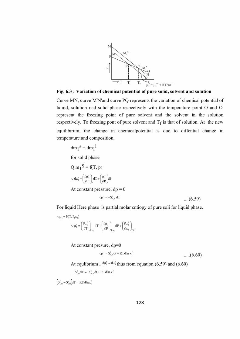
123

Tf

P

Q

N'

O

M

N

M1SO'

M'

T T0 Fig. 6.3 : Variation of chemical potential of pure solid, solvent and solution

Curve MN, curve M'N'and curve PQ represents the variation of chemical potential of liquid, solution nad solid phase respectively with the temperature point O and O' represent the freezing point of pure solvent and the solvent in the solution respectively. To freezing pont of pure solvent and Tf is that of solution. At the new

equilibirum, the change in chemicalpotential is due to diffential change in temperature and composition.

dm1s = dm1l

for solid phase

Q m1S = f(T, p)

dP

PdT

Td

s1

P

s1s

1

At constant pressure, dp = 0

dTS–d sm,

s1 ... (6.59)

For liquid Here phase is partial molar cntiopy of pure soli for liquid phase.

)xP,T(P 11l1

P,T1

1

x,T

1

x,P

11 x

dPP

dTT

11

At constant presure, dp=0

11

m,1 xlnRTddtSd .....(6.60)

At equlibrium , 1

S1 dd thus from equation (6.59) and (6.60)

– 1m,1

Sm,1 xlnRTddtSdTS

1s

m,1m,1 nxRTddTS–S

124

DSfus = THfus

, (DHfus= molar heat of fusion)

1xd = dT.

RTH

2fus

... (6.61)

Integeating equation (6.61) with the limit

from x1l = 1 to x1l = x1 and T = T0 to T = Tf

1

x

1xnd1

= f

0

T

T 2fus

TdT

RH

lnx1 =

0f

fus

T1–

T1

RH–

... (6.62)

= 0f

f0fus

TTT–T

RH–

... (6.63)

Tf= fus0

0

H/nxRT–1T

= fus20

0

H/xRT1T

If the mole fraction of solute gets increased, Tf decreases

If the solution is very dilute then lnx1 = – x2

If T0 = T02 , equation (6.63) reduced to the following equation.

f2

0

fus2 T.

RTHx

... (6.64)

DTf=2

fus

20 x

HRT =

21

2

fus

20

nnn

HRT

... (6.65)

Since DTf depends only on the amount of the solute i.e. n2 thus it is a colligative

property. If m is the molality of the solution, M1 is the molecular weight of the

solvent then

1000mM.

HRTT 1

fus

20

f

= fus

120

H1000MRT . m ... (6.66)

If kf= fus

120

H1000MRT then

DTf = kf. m ... (6..67)

Here Kf is the molal freezing point constant or cryoscopic constant of the

solvent.

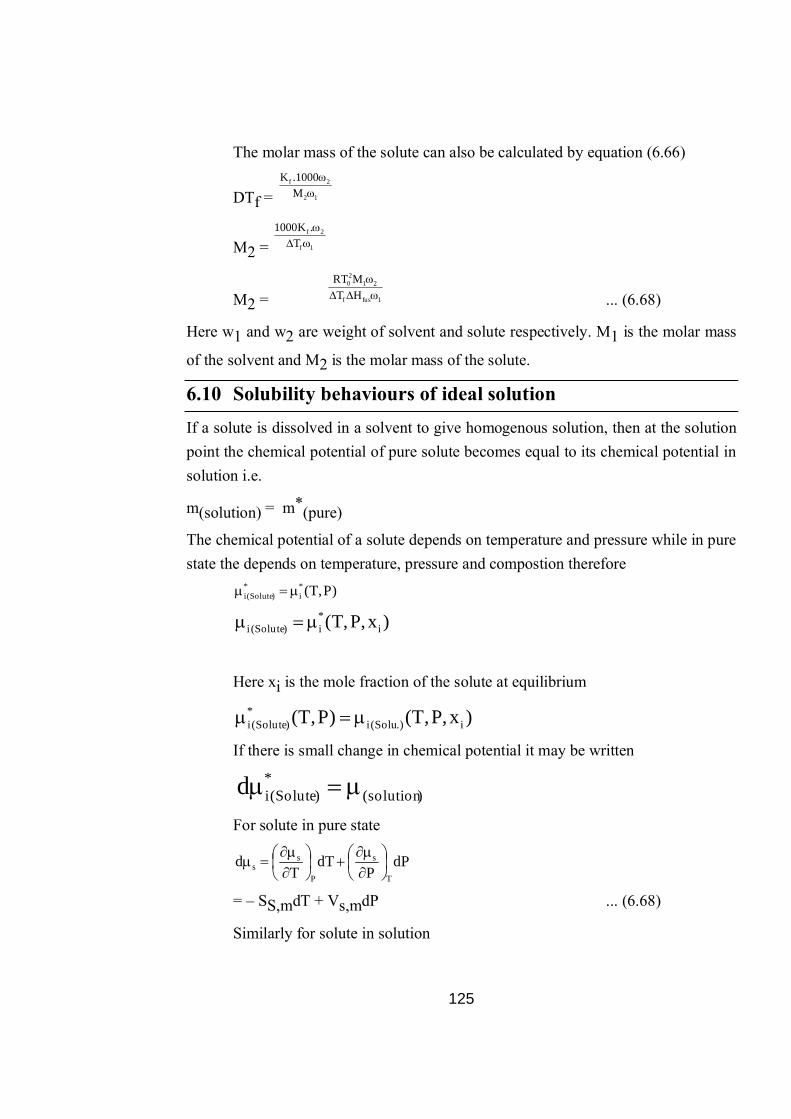
125

The molar mass of the solute can also be calculated by equation (6.66)

DTf = 12

2f

M1000.K

M2 = 1f

2f

T.K1000

M2 = 1fusf

2120

HTMRT

... (6.68)

Here w1 and w2 are weight of solvent and solute respectively. M1 is the molar mass

of the solvent and M2 is the molar mass of the solute.

6.10 Solubility behaviours of ideal solution If a solute is dissolved in a solvent to give homogenous solution, then at the solution point the chemical potential of pure solute becomes equal to its chemical potential in solution i.e.

m(solution) = m*(pure)

The chemical potential of a solute depends on temperature and pressure while in pure state the depends on temperature, pressure and compostion therefore

)P,T(*i

*)Solute(i

)x,P,T( i

*i)Solute(i

Here xi is the mole fraction of the solute at equilibrium

)x,P,T()P,T( i.)Solu(i

*)Solute(i

If there is small change in chemical potential it may be written

)solution(*

)Solute(id

For solute in pure state

dP

PdT

Td

T

s

P

ss

= – SS,mdT + Vs,mdP ... (6.68)

Similarly for solute in solution

126

i

P,Ti

s

x,T

s

x,P

ss dx

xdP

PdT

Td

ii

= –Ssl, m dT + Vsl, m dP + i

P,Ti

s dxx

... (6.69)

If pressure is constant the equation (6.68) ad (6.69) may be written as

dmS = –SS, mdT ... (6.70)

dmSl = –Ssl, mdT + i

P,Ti

s dxx

... (6.71)

At equilibrium

dms = dmsl

From equation (6.70) and (6.71)

–Ss,m dT = –Ssl, mdT + i

P,Ti

s dxx

DSm.dT = i

i

s dxx

... (6.72)

dT

THdx

x 2P,T1

s

...(6.73)

mequalibriuat0G In the ideal situation the chemical potential of the solute is

mS = ms* + RTlnxi

iP,Ti

S

xRT

x

... (6.74)

From equation (6.73) and (6.74), we get

dT.

RTnxd 2

mi

... (6.75)

Here DH may be considered as heat of fusion which is equivalent to molar entholpy change when a solution is prepared by dissolving solute in a solvent.

On integrating equation (6.75) with in the limits

127

lnxi =

T1–

T1

Rnx

e

fusi

... (6.76)

Here Te is either the temperature at equilibrium or the melting point. This expression

is also known as ideal solubility. If the solubility of an solute is expressed in mole fraction at defininte temperature, then it would be the same in all the solvents with which it form an ideal solutions. 6.2 Choose the correct alternative

a) Nodal freezing point constant is also called as ………………….(calligature property/Crysocopic constent) b) Tj decreases, as the mole protion of solute (increased dereased) c) B lullometrere constant is mdal (F.B./B.P.) d) Free energy of mixing is always ………………(negative/positive)

6.11 Oanosis When the solvent is aparted from the solution by the semipermeable membrane then the solvent molecules more from its higher concentration to its lower concentration to equalise it. This phenomenon is known as ormosis. Since the vapour pressure as well as the chemical potential of the solvent is higher than that of the solution, so the ivnolvement of solvent indecule occurs to equalised the chemical potential on the both sides. The pressure caused due to the movement of solvent moecules on the solution side is known as somotic pressure (II) or in other words the excess pressure applied over a given oslution so as to stop the flow of solvent molecules is also known as osmotic pressure. Osmotic pressure depends on the concentration of solution.

Osmans phenomenon can be understood by the experiment as shown in the figure 6.4

- - - - - - - - - - - - - - - - - - - - - - - - - - - - - - - - - - - - - - - - -- - - - - -- - - - - - - - - - - - - - - - - - - - - - - - - - - - - - - - - - - - - - - - -- - - - - -- - - - - - - - - - - - - - - - - - - - - - - - - - - - - - - - - - - - - - - - -- - - - - -

- -- -- -- -- -- -- -- -

- -- -- -

osmotic = (pressure)

Solvent Solution

Semipermeable membrane Movement of solvent molecules

Fig 6.4 Osmosis and Osmotic pressure

128

The chemical potential of the solvent (Ms) is always greater than that of the solution

(Mse) before the osmons phenomenon occur i.e.

mS> mSl

Due to the concentration gradient, the movement of solvent molecules occurs till the chemical potential on both the sides become equal. If P is the pressure on the solvent then the pressure on the solution would be (P+ p) at the equlibrium. Thus

mS (T, P) = mSl(T, P + p, x2)

mS* = mSl

Here mS* = chemical potential of the pure solvent

The chemical potential of the solvent in a solution is

mSl = f(T, P, x1)

mSl = 1

P,T

s

x,T

s

x,P

s dxT

dPP

dTT

11

... (6.77)

If dT = 0

1P,T1

s

xRT

x

1* nxRT

SS VP

1

*SS nxRTddPV ... (6.78)

Integrating equation (6.78) with in the limits

x1 = 1 to x1 = x, P = P to P = P + p,

to m = m* [T, (P + p) x2] in solution +

RT lnx1 = TP

P

*dPV–

= – V*(P + p – P) = – pV* ... (6.79)

For dilute solution ln(1 – x2) = – x2

pV* = x2RT

pn1V* = n2RT ... (6.80)

129

pV = n2RT

p = C2RT

2

2 CVn

pV = RT

2

2

m2 = RTV

2

.... (6.81)

Thus the molar mass of a solutse can be calculated from equation (6.81). The biological significance of osmoris is very pronounced. Isotonic solution are those solution which have the same osmotic pressure. Normal saline (0.84% NaCl) are isotonic with the contents of red blood cells solution from which blood cells can extract water (are said to be hypotonic) while the solution in which blood cells shrink are said to be hypertonic. The osmotic pressure depends on the number of moler of solute thus it is a colligative property.

6.12 Summary This unit describes the partial molar porperties in detail and different forms of Gibbs Duhem equations are derived. Partial molar free energy and its various with temperature and pressure is also described. Different colligative properties are described and their respective expressions are also derived ther modynamically. The application of the various concepts are also described particularly with reference to chemical or biological systems.

6.13 Glossary

Colligatrue : Which depend only on number of particles of the solute in solution.

Boiling point : Temperature at which upour preseere become equal to atnosphase pressure.

Partial molar quantity – rate of change of property with change in amount component

Chemical potential : Change in gibbs free energy with change in male component.

130


6.1 a) –SI b) VI c) –sdt d) decrease

6.2 a) cryecospic Content b) increased c) B.P d) negative

6.14 Review Questions 1. What are partial molar properties? Explain derive Gibbs Duhem equation.

2. What is chemical potential. Discuss its variation with temperature and pressure.

3. What do you understad by Ebulliometric constant? How the molar mass of a solute can be determined by elevation in boiling point?

4. What do you understand by depression in freezing point. Describe the expression for it the modynamically.

5. What is meant by osmosis phenomenon? Derive the expression for the osmotic pressure?

6. What are isotomic, hypertonic and hypotonic solution. Illustrate your answer by taking examples of each?

6.15 References and suggested reading 1. Thermodynamics by S. Glasston

2. Thermodynamics by R.P. Rastogi and R.Ri Murra

3. Physical Chemistry by Khopkar

4. Physical Chemistry by Castellan

131

Uni - 7 : Quantum Chemistry Structure of unit

7.1 Objective

7.2 Introduction

7.3 Classical Mechanics

7.4 Black Body Radiation

7.5 Quantum theory of Radiation

7.6 Photoelectric effect

7.7 Dual nature of matter

7.8 Heisenberg's Uncertainty principle

7.9 Compton effert

7.10 Introduction to Qunatum Mechanics

7.11 The Wave Equation

7.12 The Schrodingers wave equation

7.13 Operators

7.14 Postulates of Quantum mechanics

7.15 Solution of Schrodinger wave equation for simple systems

7.16 Atomic orbitals

7.17 Summary

7.18 Glossary


7.19 References and suggested reading


7.1 Objectives

As the knowledge of the principles of quanntum mechanics has become the necessry to understand the basic concepts regarding occurence of chemistry reactions, atomic and molecular orbited, digeneracy etc. So the objective of this unit is to

132

1. Acknowledge the importance of quantum mechanics

2. Unable to understand the mathematical concepts involved in it.

3. Learn the basic concept of qunatum mechanics, operators, normalisation, orthogonality etc.

4. Derive the schrodinger wave equation and its solution applied to different systems

7.2 Introduction

This unit describe the historical development of quantum mechanies and the mathematical concept involved in it. It deals with the nature of matter, photoelectric effect, compoton effect, Heisnberg's uncertainty principles, which further confirm the particle nature of radiation. The chapter also deals with Basic postulate of quantum mechanics, schrodinges wave equation and its solution for different systems like particle in a box, hydrozen like atoms etc.

7.3 Classical Mechanics (Newtonian Mechanics)

Classical mechanics is based on Newton's law of motion. It explained all the phenomenah related to motion and energy of large size objects or macroscopic particles, when it was applied to small particles or microscopic particles like electrons atoms, molecules etc, then it could not explain he discrete sets of values of energy. Which were obtained simultaneously. For example according to classical mecwanics, the position and velocity of a particle may be determined simultaneously but was contraduct by Heisen Berg's uncertainty principle Planker's theory states that the emission or absorption of energy is always in the form of packets of energy i.e. quanta. Thus the new system of mechanics was introduced to understand the concept of quantization which is known as qunatum mechanics. Now the origin of qunatum theroy will be breifly discussed.

7.4 Black Body Radiation

When the radiant energy falls on blackened metallic surface, the energy is almost completely absorbed. Different solids emit radiation at different rates at the room temperature. Black body is also a perfect radiator. Usually a hollow enclosure having a small hole wated inside with Lamp block may act as blackbody Radiations energing from it is called black body radition and the radiations emitted per unit surface area i.e., the intensity of radiations depends only on the temperature and is

133

independent on the nature of solid. However, the energy emitted by a black body at any temperature is neither confirmed to a single wavelength and has uniformly distributed. The correclation between energy density and wavelength at different temperature is depicted in figur 7.1

7.5 Quantum theory of Radiation

The nature of spectral distribution curves of black body radiations could not be explained by classical mechanies. The problem was solved by Max Planck in 1900 on the basis of quantum theory of radiation. According to planck.

(i) Energy is emitted or absorbed discontinously in the form of packets of energy called quantum.

(ii) Each quantum is associated with a definite amount of energy i.e. E = h . Here E is the energy, is the frequency of radiation and h is the planak's constant. The

numerical value of h is 6.626 x 10-34 J.

(iii) A body can emit or absorb energy only in whole number multiples of quantum i.e. 1h , 2h , 3h , .....nh . This is known as qunatizatiion of energy.

On the basis of this theory, Planck deduced expression for the energy El radiaties by

a black body at wave length as

1–kT/hc5 e1.hc8E

. .. (7.4)

This is known as Planck's radiation law

7.6 Photo electric effect

(i) Allert Einstein undertand the importance of Planck's theory and explained the photoelelctric effert. When a beam of elactromagnetic radiation of a particles frequency falls on a metal, the electrons are eemitted by it.

(ii) As the temperature increase, the position of maximum shifts towards lower wavelength.

(iii) Higher the temperature more pronounced is the maximum.

(iv) The area under the curve increases with the increase in temperature Stefan found that the total amount of energy radiated per unit area per unit time by a black body is directly propertional to the fourth power of the absolute temperature T i.e.

134

Wave length

T4

T3

T2

T1

T < 1 T < T <T2 3 4

Energy density

Fig. 7.1 : Variation of energy density with wave length at different temperatures

E T4 ----- (7.1)

This is known as Stefan - Bollzmann's law

(v) The wave length ( m) where the emilttance is maximum is inversely proportioanal to the absolute temperature

T1

m ... (7.2)

lmT = b ... (7.3)

Here b is known as Wien's constant and

This is called as photo electric effect. The significant observations concering photoelectric effect are as follows -

(i) Photoelectric emission of electron is possible only with a beam of certain minimum frequency i.e. threshold frequency.

(ii) The kinetic energy of the emitted electron increases on increasing the frequency and reamins unaffected on increasing the intensity of incident light.

(iii) The number of ejected electron from the metal surface increases with increasing the intensity of incident radiations.

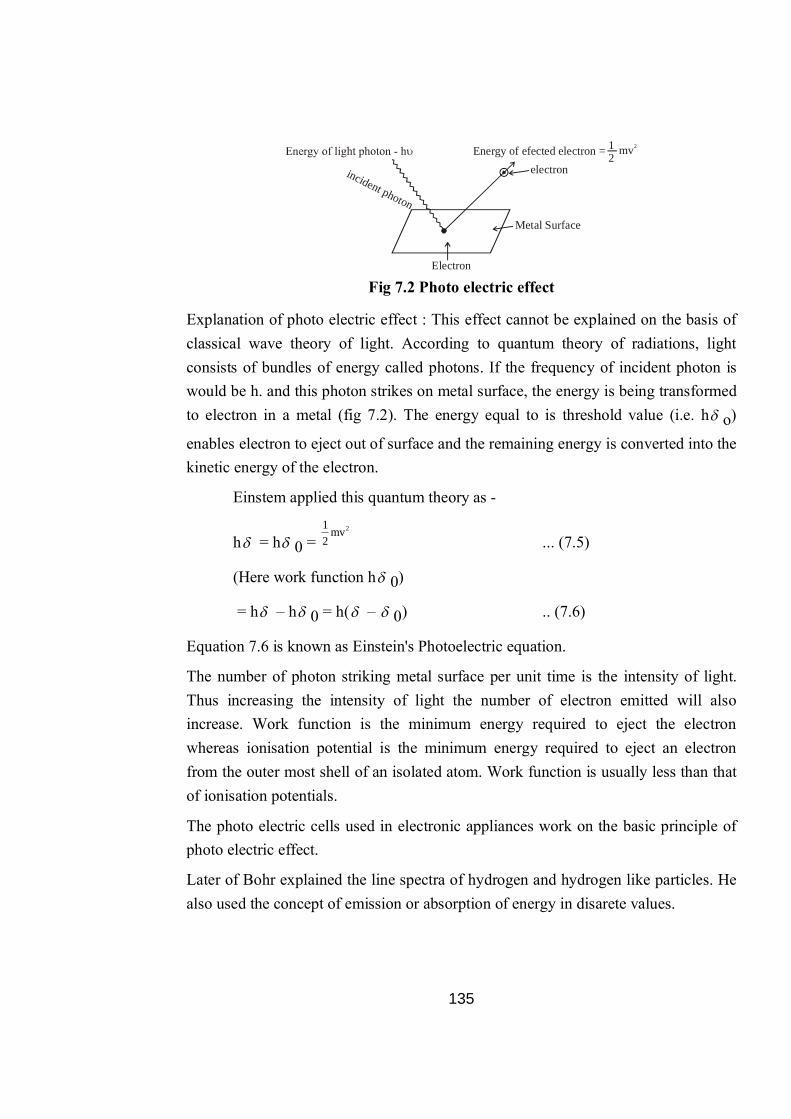
135

Energy of efected electron = mv212

electron

Metal Surface

Electron

incident photon

Fig 7.2 Photo electric effect

Explanation of photo electric effect : This effect cannot be explained on the basis of classical wave theory of light. According to quantum theory of radiations, light consists of bundles of energy called photons. If the frequency of incident photon is would be h. and this photon strikes on metal surface, the energy is being transformed to electron in a metal (fig 7.2). The energy equal to is threshold value (i.e. h o)

enables electron to eject out of surface and the remaining energy is converted into the kinetic energy of the electron.

Einstem applied this quantum theory as -

h = h 0 = 2mv

21

... (7.5)

(Here work function h 0)

= h – h 0 = h( – 0) .. (7.6)

Equation 7.6 is known as Einstein's Photoelectric equation.

The number of photon striking metal surface per unit time is the intensity of light. Thus increasing the intensity of light the number of electron emitted will also increase. Work function is the minimum energy required to eject the electron whereas ionisation potential is the minimum energy required to eject an electron from the outer most shell of an isolated atom. Work function is usually less than that of ionisation potentials.

The photo electric cells used in electronic appliances work on the basic principle of photo electric effect.

Later of Bohr explained the line spectra of hydrogen and hydrogen like particles. He also used the concept of emission or absorption of energy in disarete values.

136

7.7 Dual nature of matter

Einstein (1905) suggested the dual character of light i.e. wave as well as particle nature. The phenomeana of diffeaction, interfernce etc. were explained on the basis of wave nature and photoelectric effect comptan effect could be explained on the basis of particle nature. De Broglie who was awarded Nobel prize in 1929, proposed dual character (as wave and as particle) of matter.

Derivation of Broglie's equation

The wave length of the wave associated with any material particle like clectron can be calculated by analogy with photon as follows -

If the wave nature of photon is assumed then its energy can be given according to Planck's qunatum theory

E = h ... (7.7)

Here is the frequency of wave and h is plank's constant.

If the photon possesses a particle character then the energy is given by Einstein's equation as

E = mc2

c 2mchc

... (7.8)

Combrining both the expressions for energy from equation (7.7) and (7.8) we get

hu = mc2

mch

\ mch

Ph

(7.9)

137

Here p = mc be the momentum of the particle.

Equation (7.9) is known as de Broglie equation and is de Broglie wave length. It relates the particles character with the wave character of the matter. The significance of above equation (7.9) implies only for microscopic particles not for macrosopic ones. It can be explained by taking example of a ball and electron.

Let us suppose that the mass of a ball is 0.1 kg and its velocity is 65m S-1

According to de Broglie's equation

m10

ms651.0Smkg1062.6 34–

1–

1–234–

The value of its wave length is too small for simple observation. But if we ake on

electron whose mass at rest is 9.11 x 10–31 kg moving with the speed same as in case of ball then the value of would be

Å10m10

651011.9Smkg1062.6 55–

31–

1–234–

This value of could measured experimentally very easily.

Experimental verification of character de Broglie's relation ( ) Verification of wave character.

Davison and Gremer varified de Broglies's Hypothesis experimantaly in 1927 when the beam of electrons ensitted from a hot filament was allowed to strike nickle plate. The electron were accelerated the surface of by a potential ranging between 40 and 68 volts before striking the plate. It resulted in production of diffraction patterns on the photographic plate, similar to those obtained by x-rays under similar conditions. Since x-rays possess wave charecter so it gave direct evidence for the wave character of electron as well. The wave length determined from the diffraction pattern is found to be very nearly the same as calculated from the De-broglie equation.

(ii) Verification of particle character

The particle charpcter of the eleetion is prooved bu different experiments as follows :

(a) When an electron strikes a zinc sclphipn sereem, scintillation spark is localized and the character prooves the particle character of electron.

138

(b) Thomson's experiment for determination of the ratio of change to mass (i.e e/m) and mulliken oil drop experiment for determination of charges on electron confirms the particle character of electron.

(c) Photo electric and compton effect also prove the particle nature of radiation.

7.8 Heisenberg's Uncertainly principle

Heisenberg, a German Physicist in 1927 gave a principle which states that it is not possible to determine precisely both the position and the momentum of a small moving particle. For an electron moving in x-direction , the Heinsberg unscertainty principle is expressed mathematically, as

(x) (px) 4h

..... (7.10)

The product of the uncertainty in the position (x) and the consertainty in

momentum (px) is always constant and is either equal or greater than 4h

If x is very small i.e. the position of a particle is known more or less exactly, p would be large i.e. uncertainty with regard to momentum will be large. Similarly If momentum is measured exactly, the uncertainty of position will be large.

Derivation

Let an incident photon strikes an electron at M point in the x-direction and seatter along MN or MO direction. Along MN direction, the momentum is given as

sinh

Thus the momentum imparted to the electron in the x-direction will be

Px = h

+

sinh–

=

sinh–h

... (7.11)

The momentum impartied to the electron by seattering of photon along Mo would be

sinhhP '

x ... (7.12)

The uncertainty in the measurement of momentum of an electron is given as

139

incident

Photon x axis

Fig. 7.3 : Source Heisenbeeg's principle Seattering of electron by photon along x - axis.

Substuting the value of px1and px from equations (7.11) and (7.12) in equation (13)

respetively.

sinhhP

–

sinh–h

DP =

sinh2

... (7.14)

According to law of optics, the minimum distance between two points (Dx) is given as

Dx =

sin2 ... (7.15)

Multiplying equation (7.14) and equation (7.15) we get

DP.Dx = h

sin2.sinh2

or more accurately

4hx.P

This represents the mathematical form of Heinsnberg's uncertainty principle.

7.1 Fill in the blanks a) ……………give quenteem theory of radiation.

b) According to stejan baltmann lour, E is diretly proportion and to pour of

temperature.

c) Kinetre energy of emitted electron remain --------on increasing the

intensity of incident light.

d) According to Heisenberg uncertainity principle position and -----------of a

particle con not be determined is multoneousely.

140

7.9 The Compton effect

The particle nature of electromagnetic radiation was further supported by the experiments performed by Compton in 1923. He found that when monochromatic beam of x-rays is allowed to fall ono surface of light element (low weight) the wavelength of scattered x-rays increases as compare to that of incident x-rays and thus the frequency of seattered radiation decreases. As scattering is caused by electrons any is this may be explained on the basis of interaction of x-rays with the clectrons. The increase in wave length of x-rays due to scattering from the surface of an object is known as compton effect.

If the wavelength of incident x-rays is l and the energy of the photon is h.. then the

momentum will be ch

where c is the velocity of light. Similarly if is the

wavelength of seattered x-rays then the respective momentum would be c'h

. Similarly considering the momentum of electron after collsinon and applying law of conservation of energy and momentum, the increase in wavelength can be calculated as

D = l' – l = )cos–1(

cmh

0

... (7.16)

Here mo is the restmass of electron and q is the angle between the incident and

scattered x-rays. The increase in wave length i.e. Dl is known as compton shift which is independent of wave length of incident x-rays. It only depends on the angle of scattering (q). Thus three cases may be considerd as follows

Case I When q = 0° i.e. the seattered radiation is parallel to the incident radiation

Dl = 0)1–1(

mch

Case II When q = 90° i.e. the scattered radiation is perpendicular to the incident radiation

D = mch)0–1(

mch

= 2.42 pm

Case III When q = 180° i.e. the radiation is seattered in a direction opponite to the incident radiation.

D = )1(––1

mch

= mch2

= 4.84 pm

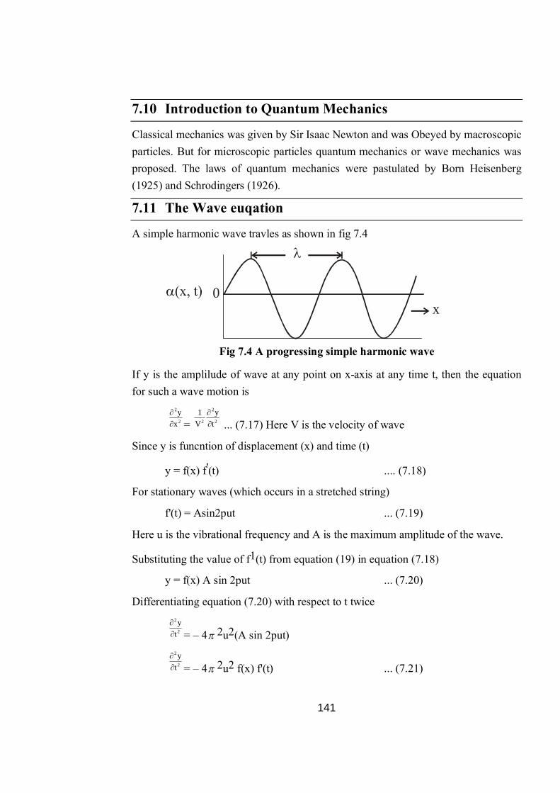
141

7.10 Introduction to Quantum Mechanics

Classical mechanics was given by Sir Isaac Newton and was Obeyed by macroscopic particles. But for microscopic particles quantum mechanics or wave mechanics was proposed. The laws of quantum mechanics were pastulated by Born Heisenberg (1925) and Schrodingers (1926).

7.11 The Wave euqation

A simple harmonic wave travles as shown in fig 7.4

x0

Fig 7.4 A progressing simple harmonic wave

If y is the amplilude of wave at any point on x-axis at any time t, then the equation for such a wave motion is

2

2

xy

= 2

2

2 ty

V1

... (7.17) Here V is the velocity of wave

Since y is funcntion of displacement (x) and time (t)

y = f(x) f'(t) .... (7.18)

For stationary waves (which occurs in a stretched string)

f'(t) = Asin2put ... (7.19)

Here u is the vibrational frequency and A is the maximum amplitude of the wave.

Substituting the value of f1(t) from equation (19) in equation (7.18)

y = f(x) A sin 2put ... (7.20)

Differentiating equation (7.20) with respect to t twice

2

2

ty

= – 4 2u2(A sin 2put)

2

2

ty

= – 4 2u2 f(x) f'(t) ... (7.21)

142

Differentiating equation (7.18) twice wrt t we get

2

2

xy

= 2

2

x)x(f

. f'(t) ... (7.22)

Substituting the values of 2

2

ty

and 2

2

xy

from

equation (7.21) and (7.22) in equation (7.17)

2

2

x)x(f

f'(t) = )t('f)x(f4

v1– 22

2

2

2

x)x(f

= )x(f

v4– 2

22

... (7.23)

This euqation (7.23) exhibits the variation of amplitude function f(x) with x and also does not depend on time

Since v =

Equation (7.23) may be written as

)x(f4–

x)x(f

22

2

... (7.24)

7.12 The Schrodinges wave equation

Equation (7.24) may be extended to the wave motion in three dimensions. The amplitude function f(x) may be replaced by ....(x,y,z) and thus the equation is

2

2

2

2

2

2

2

2 4–zyx ... (7.25)

According to de Broglie hypothesis

equation (7.25) may be written as

2

2

2

2

2

2

2

2

2

)mv(h4

zyx

2

222

2

2

2

2

2

2

hvm4

zyx ... (7.26)

Further the total energy (E) of the particle = Kinetic energy + Potential energy

E = 2mv

21

+ v (Here v is the potential energy of the particle)

2mv

21

= E – V

143

mv2 = 2(E – V) ... (7.27)

From equation (7.26) & (7.27)

0

h)v–E(m8

zyx 2

2

2

2

2

2

2

2

... (7.28)

Equation (7.28) is known as Schrodinger wave equation

2

22

h)v–E(m8

= 0 ....( 7.29)

2

2

2

2

2

22

zyx

2 is known as Laplacian operator

2

22

h)v–E(m8–

–

V–E

m8h 2

2

2

EV

m8h– 2

2

2

EV

m8h– 2

2

2

... (7.30)

If V

m8h–H 2

2

2

Then equation (7.30) may be rewritten as

H = E ... (7.31)

Here H is Hamiltonian operator

Physical Significance of wave function ( and 2)

y represent the ampitude of the electron wave. The product of with its complex conjugate i.e. has physical significance. Since most of the wave functions in atomic

or molecular structure problems contain real terms only. The value of 2 gives the measure of electron change density at any point around the muclens. The statistical

inter pretation of the electron wave function shown that the value of 2 represent the probability of finding the electron at any point at particular time.

The properties of wave function are as follows -

144

(i) must be single valued and finite i.e. for each value of the variables x,y and z there in only one value of .

(ii) must be continous i.e. there must not exist any sudden changes, as its variables are changed.

(iii) For bound states, must varish at infinity i.e. must become zero infinity.

When all there conditions are satisfied then the wave function is said to be well behaved wave function.

Normalized and orthogonal wave function

The schrodinges wave equation is a homogenous differatial equation whose solution gives a value for . *dt is equal to the prolalility of finding the particle (electron) in the small volume dT and gives the total probalility in the space which shoule be equal to unity i.e.

* 1dt (Here dT = dx. dy. dz)

A wave function which satisfies an equation (7.31) is said to be normalised and this condition is called nomalisation conditionlet i and j are two different given functions

(corresponding to eigen values Ei and Ej respectively) and if the following condition

is to be satisfied (7.33) then the wave functions are said to be orthogonal to each other. Such a condition is called conditions of orthogonalies of wave fucntion. Such wave function which are normalised as well as orthogonal are called orthonormal.

1dTji if i = j = 0 ------------------(7.33)

7.13 Operators

An operator is a mathematical instructions of procednre to be carried out on a function so as to get another function.

(operator) × (function) = (Another function)

The function on which the operator is carried out is called and operator is not exactly multiplied with the function but only operator written has no significance. If a number is put under it then it will transform it this its square root. The concept of operator may be understand by taking few examples

(i) )x(sin

dxd

= cos x

145

Here dxd

the differentiation with respect to x is an operator, sin x is the operand and cos x is the result of operation.

(ii) dxd

(ax3) = 3ax2

Here dxd

is operator, ax3 is an operand and 3ax2 is the result

(iii) 4x = x2

Here (square root) is the operator, x4 is an operand and x2 is the result.

Usually operator is represented by putting the symbol (^) over it. For example

Hamitonian operator is represented as ^H

Algebra of operators : Although the operators do not have any physical meaning they following certain rules follow similar to those of algelra. They can be added, subtracted, multiplied and have some other properties also.

Addition or Substraction of operators

The addition or substraction of operators yields new operators. For example if and are two different operatos and f(x) is the operand then

( Â

^B )f (x) + ^

A f(x) ^B f(x)

Multipicational of Operators

If and are two operators and f(x) is the operand then the multiplication means the operation will take place one after other and the order of operation would be from right to left.

Â

^B f(x) = ^

A (f(x) = ^B f '(x) = g(x)

if Â = 2x2, ^

B = and dxd

f(x) = ax2 then

Â

^B f(x) = 2x2. dx

d

(ax2) = 2x2 . 2ax = 4ax3

Commutative operators

When a series of operations are performed on a function, the result depends on the sequence in which the operations are performed. But if the operators are such so that the result does not depend on their order i.e.

146

Â

^B f(x) = ^

BÂ f(x)

then the operators are known as commutative and if not equal then they are said to be non commutative.

if Â = dx

d and ^

B = 2

2

dxd

For example

xsin

dxd

dxd

2

2

=

xsin

dxd

dxd

2

2

= – cos x

and are said to be commuteatue.

Linear Operators

An operator is said to be linear if the sum of two functions gives the same result which is being obtained by the sum of the operations of the two fucntions separately.

)x(g)x(fA^

= )x(gA)x(fA^^

Commutator Operator

If Â and ^

B are two operators then the difference between – is (A, B) called

commutative operator. As earlier stated if Â

^B = ^

BÂ the operatos are said to commute

and hence [ Â – ^

B ] = 0. Hero 0 is called zero operator.

Laplacian Operator (2)

Laplacian operator is three dimensional operator. It is denoted as 2 (del squared) and is

2

2

2

2

2

22

zyx

The schrodinger wave equation has three dimension operator –

0)V–E(

hm8

zyx 2

2

2

2

2

2

2

2

It can be replaced by 2 as

0)V–E(

hm8

2

22

Hamiltonian Operator

It is denoted by

H and is given as

147

V

m8h–H 2

22^

(From schrodingre wave equation)

EH^

Here is eigen function and E is called eigen value. Thus the schrodinger wave equation is explained as

(Energy operator) (Wave function) = (Energy) × (Wave fucntion)

Hermitian Operator

If an operator has two eigen function and if both are real, then

QdT)A(dT)QA( ^^

Or QdT)A(dT)QA( ^^*

Here * is the complex conjugate of and dT is the small volume of space in which

the function is defined, then the operator ^A is called Hermitian operator.

Eigen values and Eigen functions

If an operator ^A operators on a well behaved function to give the same function but

multiplied by a then the constant is called the "eigen value" of the operator, the function is called the "eigen function" and the equation is eigen value equation.

operator × function = constant value × fucntion

for example dx)e(d x2

= 2e2x

Here 2 is eigen value and e2x is eigen function of the operator dxd

7.14 Postutates of Quantum mechanics

Few mathematical formalism of quantum mechanics which are also known as its basic postulates are stated below -

First postulates : The state of a microsystem at any time is described in terms of a function of partition coordinates i.e. wave function, (x,t)

148

Second postulate : The wave function and its first and second derivaties i.e. dxd

or

2

2

dxd

are continous, finite and single valued for all values of x. Further the wave function (x,t) must be normalised. Thus

1dT2

or 1dT*

Third postulate : A physically observable quantity can be represented by a Hermistian operator i.e. must follow the Hermitian condition.

Fourth postulate : The allowed values of an observable a are the eigen values in the operator equation.

111^ aA

Fifth postulate : The average value <A> of an observable A corresponding to the

operator ^A is given as

< A > =

dT

dTA*

*

Sixth postulate : The quantum mechanical operators corresponding to the observable are formed by writing the classical expressions in terms of the variables and converting the expressions to the operator as given in table 7.1

Table 7.1 : Quantum Mechanical operators for evaluating various classical variables.

Classical Variable

Position (x)

momentum alongx-axis (P )x

momentum (P)

Kinetic energy

Potential energy

Total energy

x multiplication by x

derivative wrt x and multiplying by

derivative wrt x, y and z axis andmultiplying by

derivative wrt x, y and z axis andmultiplying by

Potential energy along x, y and z axis

Adding Kinetic energyand potential energy

x

Px

P

T

V

E

Quantum Mechanical operator

Operator Operation

149

If the particle moves in all the three directions then yx , yy and yz will be

considered and the total energy E may be given as

E = Ex + Ey + Ez

7.15 Solution of the schrodinges wave equation for simple system

The Schrodinges wave equation may be solved for simple systme like particle in one dimensiond box, particle free particle in three dimensional box, the hydrogen atom etc.

7.15.1 Free Particle System

Free patricle may move anywhere in the space without any potential barries. It is allowed to move linearly (along x-axis). Then the Hamiltonian is give as

V

dxd.

m8h–H 2

2

2

2^

... (7.34)

The schrodinger equation for the free particle may be written as

0E

hm8

dxd

2

2

2

2

... (7.35)

The general solution of equation (ii) is

= A sin kx + B cos kx ...... (7.36)

Here A and B are arlitrary constants

R2 = 2

2

hmE8

The equation (7.35) is related to the simusoidal wave and can be converted into more useful form

= Ceikx + De–ikx ..... (7.37)

Here C and D are constants

Since e+ikx are eigen functions of the linear momentum operator c2h dx

d . with

eigenvalues

2kh

which is equal to mE2 (classical wave length of the particle

150

momentum), Therefore the wave length of the particle ( ) is given by the following equation

l = xPh

= mE2h

... (7.38)

If D = 0 then y = Ceikx ... (7.39)

(for a particle wave braveling in +x direction)

7.15.2 Particle in a box

This application is the simplest one as applied to translational motion of a particle in space. First of all, it will be solved for the particle in one dimensional box and then the expression for three dimensional box will be derived.

Particle in one dimensional box

If a particle of mass in si confirmed to move in one dimensional box from x=0 to x=a. The potential energy inside the box in taken as zero and outside the box is infinite. The model is also called as the particle in potential well as shown in fig 7.5.

V = V =

aV = 0

x = 0 x = ax

v

Fig. : 7.5 : Particle in one dimensional box

The schrodinger wave equation for one dimension is

0)V–E(

hm8

dxd

2

2

2

2

... (7.40)

Outside the box as V=, thus the equations beomces

0)–E(

hm8

dxd

2

22

Edxd.

m8h– 2

2

2

2

Similarly the schrodinges equation inside the box i.e.

E0dxd.

m8h– 2

2

2

2

(Here V = 0)

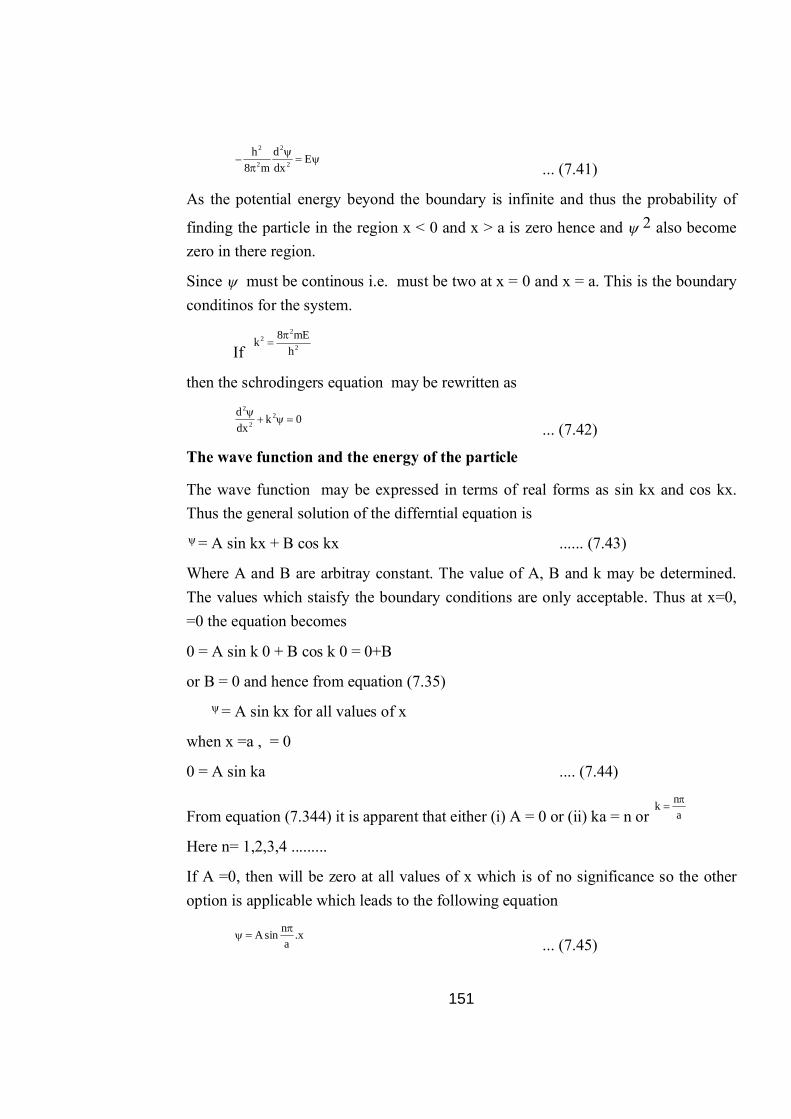
151

Edxd

m8h– 2

2

2

2

... (7.41)

As the potential energy beyond the boundary is infinite and thus the probability of

finding the particle in the region x < 0 and x > a is zero hence and 2 also become zero in there region.

Since must be continous i.e. must be two at x = 0 and x = a. This is the boundary conditinos for the system.

If 2

22

hmE8k

then the schrodingers equation may be rewritten as

0k

dxd 2

2

2

... (7.42)

The wave function and the energy of the particle

The wave function may be expressed in terms of real forms as sin kx and cos kx. Thus the general solution of the differntial equation is = A sin kx + B cos kx ...... (7.43)

Where A and B are arbitray constant. The value of A, B and k may be determined. The values which staisfy the boundary conditions are only acceptable. Thus at x=0, =0 the equation becomes

0 = A sin k 0 + B cos k 0 = 0+B

or B = 0 and hence from equation (7.35) = A sin kx for all values of x

when x =a , = 0

0 = A sin ka .... (7.44)

From equation (7.344) it is apparent that either (i) A = 0 or (ii) ka = n or ank

Here n= 1,2,3,4 .........

If A =0, then will be zero at all values of x which is of no significance so the other option is applicable which leads to the following equation

x.

ansinA

... (7.45)

152

E = m8hk2

22

=

m8ha/n

2

22

= 2

22

ma8hn

... (7.46)

Applying the condition for normalisation

a

0

* 1dT substituting the value of from equation (7.45)

a

0

22 1xdxansinA

1

2a.A2

2adx.

axnsin2

A = a2

Hence the normalized wave function is given as

y a2

= x.

an

sin ... (7.47)

Quantization of energy

Substituting the value of n= 1,2,3 ... in equation (7.46) the different energy levels are obtained which are shown in figure

E1 = 2

2

ma8h

, E2 = 2

2

ma8h4

, E3 = 2

2

ma8h9

, E4 , 2

2

ma8h16

....

Since n 0, hence the minimum energy possessed by the particle in not zero but has a definite value which is called as zero point energy.

n = 4

n = 3

n = 2

n = 1

E = 16h /8ma42 2

E = 9h /8ma32 2

E = 4h /8ma22 2

E = h /8ma12 2

Fig 7.6 Energy levels for the particle in one dimensional box.

The normalised wave function are represent graphically in fig 7.7

153

n = 3

n = 2

n = 1

a

Fig. 7.7 : Form of y waves of a particle in one dimensional

It is evident from the graph that for n=1 there is no node. As n increases number of nodes also increases. The no. of modes = n-1. The wave function is symmetric when n is odd and is antisymmetric when is even forms of waves of particle in one dimensional box.

7.15.3 Particle in a three dimensional box

If a microscopic particle of mass m moving in a three dimensional box with edge of

length a and volume equal to a3. The potential energy inside the box is zero and is infinie at the boundaries and outside the box. The time independent schrodinger equation for the particle is

0

hmE8

dzd

dyd

dxd

2

2

2

2

2

2

2

2

... (7.48)

The equation may be solved by separting the variable taking as a produce of three functions y(x), y(y), and y(z), each in one variable

y = y(x) y(y) y(z) ........ (7.49)

Substituting the value from equation (7.49) in equation (7.40) and dividing the resulting equation by xyz , we get

2

2

2z

z2y

y2x

x hmE8

z1

y1

x1

... (7.50)

Since the total energy of the particle is constant hence the Result of equation (7.50) is also constant

154

If k2 = 2

2

hmE8

then equation (7.50) becomes

2

2z

2

z2

y2

y2x

2

x

k–z

1y

1x

1

... (7.50)

Thus each then on LHS of equation (7.50) must also be constant and we may write followings

2x2

2

x

k–x

1

... (7.52)

2y2

2

y

k–y

1

... (7.53)

2z2

2

z

k–z

1

... (7.54)

k2 = kx2 + ky2 + kz2 .... (7.55)

Similarly

2x

22x h

mE8k

... (7.56)

2y

22y h

mE8k

... (7.5)

2z

22z h

mE8k

.... (7.58)

Here Ex, Ey and Ez are the components of energy along x,y and z axis respectively.

E = Ex +Ey + Ez

From equation we get

0k

x x2x2

x2

... (7.59)

0k

y y2y2

y2

....( 7.60)

0k

z z2z2

z2

... (7.61)

Equation (7.59), (7.60) and (7.61) may be solved as in case of particle in one dimensional box and thus leads to the following equation.

155

x

ansin

a2 x

x

y

bn

sinb2 y

y

z

cnsin

c2 z

z

2

22x

x ma8hnE

, 2

22y

y mb8hn

E , 2

22z

z ma8hnE

Substituting the value of x, y and z from equation above equestions respectively we

get

y =

xa

nsina2 x

y

an

sinb2 y

zc

nsinc2 z

y = abc8

x

ansin x

y

bn

sin y

z

cnsin z

... (7.62)

\ E = Ex + Ey + Ez

The total energy of the particle is

E = 2

22x

ma8hn

+ 2

22y

mb8hn

+ 2

22z

mc8hn

E = m8h2

2

2z

2

2y

2

2x

cn

bn

an

... (7.63)

If the box is cubical then a = b = c and thus equation (7.63) may be written as

2

z2y

2x2

2

nnnma8hE

Putting different values for nx, ny and nz one can have degenerate energy levels.

The lowest energy of the system is given by putting the values of nx = ny = nz = 1

222

2

2

111 111ma8hE

= 2

2

ma8h3

... (7.54)

which is three times that for a particle in one dimensional box.

The corresponding wave function would be

azsin

aysin

axsin

a8

3111 ... (7.65)

The next energy level can be obtained by putting one of the quantum number 2 and the others one each.

156

E211 = E121 = E112 = 2

2

ma8h6

... (7.66)

and the wave functions

azsin

aysin

ax2sin.

a8

3211

azsin

ay2sin

axsin.

a8

3121

az2sin

aysin

axsin.

a8

3112. .. (7.67)

Such energy states which have more than one wave function for the same value of energy is called degenerate state and the phenomenon is called degenerocy. Here it has three wave functions for the same value of energy, so it would be known as triply degenerate.

The energy levels of a particle in a cubical box are shown in fig 7.5

E

Non degenerate

Triphy degenerate

Triphy degenerate 211 121 112

221 212 112

222

E = E = E =221 212 122

2

2

222 ma8h12E

E = E = E =221 121 112

Non degenerate 111

2

2

ma8h9

2

2

ma8h6

2

2

111 ma8h3E

Fig 7.8 Energy levels in a cubical box showing degeracy

7.15.4 Schrodinger wave equation for hydroden and hydrogen like atoms

Hydrogen atom is a the simplest system of one proton and one electron Hydrogen atom and hydrogen like system are characterized by a spherically symmetric potential energy which is given as

r)4(ZeV

0

2

... (7.68)

Here the potential energy is a function of r only which is same in all direction and this is independent of the spherical angular variables q and f in two particle system If

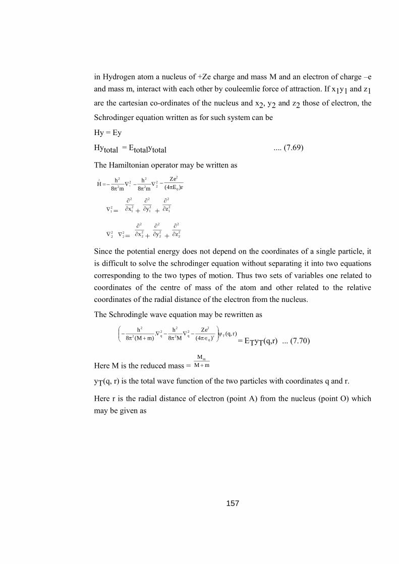
157

in Hydrogen atom a nucleus of +Ze charge and mass M and an electron of charge –e and mass m, interact with each other by couleemlie force of attraction. If x1y1 and z1

are the cartesian co-ordinates of the nucleus and x2, y2 and z2 those of electron, the

Schrodinger equation written as for such system can be

Hy = Ey

Hytotal = Etotalytotal .... (7.69)

The Hamiltonian operator may be written as

2

2

2^1m8

h–H

222

2

m8h– r)E4(

Ze–0

2

21 =

21

2

x

+ 21

2

y

+ 21

2

z

22 2

2 = 22

2

x

+ 22

2

y

+ 22

2

z

Since the potential energy does not depend on the coordinates of a single particle, it is difficult to solve the schrodinger equation without separating it into two equations corresponding to the two types of motion. Thus two sets of variables one related to coordinates of the centre of mass of the atom and other related to the relative coordinates of the radial distance of the electron from the nucleus.

The Schrodingle wave equation may be rewritten as

)r,q(

)4(Ze–

M8h–.

)mM(8h– Tr

0

22q2

22q2

2

= ETyT(q,r) ... (7.70)

Here M is the reduced mass = mMMm

yT(q, r) is the total wave function of the two particles with coordinates q and r.

Here r is the radial distance of electron (point A) from the nucleus (point O) which may be given as

158

Nucleus rA electron

z

y

x Fig. 7.9 : Ralationship between spherical and spherical polar coordinates

r = 222 zyx

From figure 7.9

x = rsinq cosf

y = rsinq sinf

z = rcosf

From equation (7.70) and above equation we get

m8h– 2

2

2

2

2222

2 sinr1sin

sinr1

rr

rr1

r4

Ze–0

2

= Ey

Here y = y(r, Q, y)

The schrodinger wave equation for hydrogen atom in terms of polar coordinates becomes

h2

sinr1sin

sinr1

rr

rr1

2

2

222

2

0.

4ZeE r

0

2

Here m is the reduced mass of electron and nucleus ne

ne

mmmm

Separation of variables

Since y is a function of three variables r, q and f thus

y(r, q, f) = R(r) Q(q) f(f) ...(7.71)

Here R(r) is the radial function and Q(q) and f(f) are angular functions. From equation (7.71) one can get three seperate equations.

drdRr

rr1 22 – +

r4ZeE

h2

0

2

2

R = 0 ... (7.72)

159

d

dsindd

sin1

-

2

2

sinm

+Bq = 0 ... (7.73)

d

dsindd

sin1

-

2

2

sinm

+BQ=0

2

2

dd

m2f = 0 ... (7.74)

Here m an b are constants

Thus the schrodinger wave equation for hydrogen or hydrogen like atoms has been separeted into three equations. Here b = e(+ 1) where = 0 or an integer (i.e. =0, 1, 2, 3, .....)

Equation (7.74) may be rearranged in the following manner

2

2

dd1

= – m2 .... (7.75)

Equation (7.75) is known as f equation

Further substituting the value of and rearranging the equations, we can get the radial equation and the q equation.

drdRr

drd

R1 2

+2

0

22

rr4

ZeEh

8

= )1(

Equation (6) is known as radial equation or R equation

ddQsin

sin1

– 0)1(

sinm

2

2

... (7.16)

Equation (7.16) is known as q equation.

Solution of f equation

f(f) =

ime

21

m = 0, ±1, ±2, ±3, ......

Solution of q equation

q(q) = )(cosP

|!m||!m|–.

212 |m|

2/1

... (7.79)

= 0, 1, 2, 3, 4 ..........

m = 0, ± 1, ± 2, ± 3 ........

m = – .... 0 ..... + =

160

Both of these functions are angular functions.

Solution of Radial equation

)r(R ,n = e–1/2 )(Le 121n

)(L 121n is Laguerre polynomials.

Thus the complete wave function of hydrogen like atoms may be written as

),,r(m,,n = )(F)(PR mm)r(,n

= )(R m.e1

)r(,n

Here n, and m are the three quantum numbers.


a) When n =4, E4 = ……….h2/8ma2

b) Qrthogonality of and can be written as…………

c)

d) schrodinger wave equation can be written as

7.16 Atomic orbitals

The quantum mechanical approach is useful in calculating the value of y for on

electron of knwon values of n, and m, y2 gives the probability of finding the electron in three dimensional space around the nucleus i.e. orbital. Depending on the value of n and different orbitals ar assigned for the electrons. Since y is a [rpdict pf radial and angular wave function, thus the shape and the size of the orbitals are decided by it

mm,,n .R The radial wave function (R) denotes the energy while angular wave function q and f denotes the shape and orientation of the orbitals. The radial probability of an electron in the concentric shells around the nucleus is given as

Radial probability = drr4R 22,n

As r increases, R2 decreases. The radial probability distribution curves for different orbitals are shown in the figurer 7.10

161

r r r r

1s3s 2p

Fig. 7.10 : Radial probability distribution curves

The radius of maximum probability is given by the peak (maximum displacement). In case of H-atom it is found to be 0.529Å, which is equivalent to Bohr's radius. If we compare 2s and 2p then it is found that 2s electron is more closer to nucleus than that of 2p. Similar bend is found in case of 3s, 3p and 3d.

The probability of finding the electron more closer to the nucleus is in the order 3s > 3p > 3d.

The angular wave function of S-orbital is given by the following equation.

q0, f0 = 41

= 21

)0m,0(

Since the angular wave function for the S-orbital does hot depend on q and f thus it is symmetrical and is of spherical shape.

Similarly the shape of p-orbitals can also be given as

q1, f+1 =

2/1

43

sinq sinf =

2/1

43

( =1, m = +1)

q1,–1, f–1 =

2/1

43

sinq sinf =

2/1

43

ry

( =1, m = –1)

q1,0, f0 =

2/1

43

cosq =

2/1

43

( =1, m = 0)

Since the angular wave function vary with x, y and z respectively, So they give the dumb-bell shape as shown in the figure (7.11)

If =2, then m = –2, –1, 0, +1, +2 and their respective angular wave function are given as

q2, –2f–2 = 2

2/1

rxy

415

162

q2, –1f–1 = 2

2/1

ryz

415

q2f0 – (3z2 – r2) 2r1

q2, +1f+1 = 2

2/1

rxz

415

q2, +2f+2 = 2

222/1

ry–x

1615

The equations of angular wave functions for d-orbitals indicate that three orbitals dxy, dyz, dxz are lying between the axes and are lying along x, y and z axes

respectively as shown in figure 7.12.

Fig. 7.11 : Shapes of Px, Py and Pz orbitals

Fig. 7.12 : Shapes of d-orbitals

7.17 Summary

In this chapter the historical development of quantum mechanics has been discussed several effects like photo electric, compton, laws regarding radiation in confirmation of it's particle nature are described. The postulates of quantum mechanies the basic terms involved are also discussed. The Schrodingers wave equation has been derived and the properties of wave function and also its physical significance are given in detail. Schrodinger wave equation has been applied to several simple systems and also being solved to get wave function and the respective energy values. The concept of degeneracy of energy levels has been explained in detail. The quantum mumbers and the shape of atomic orbitals are also described.

163

7.18 Glossary

Intensity of radiation : radiation emitted per unit surface area.

Dual character : Wave as well as particle nature

Compton effect : wavelength of scattered x rays increases from the syrfare of an alyeit.

Commutative operator: Result of the operator does not depend on their order.

Linear operator : siem of two junctions guies the same result.

Answer to key assessment Questions

7.1 a) Max Planck b) 4th c) un aflected d) momentum

7.2 a) 16 b) 41 41dC=o b) E d) bn2m/n2 (E-V)


1. What is black body ? Discuss the energy distribution for black body radiation at different temperature.

2. State and explain Wein's displacement law

3. Discuss photoelectric effect

4. What do you understand by de Broglie hypothesis?

5. Discuss photoelectric effect.

6. State Stefan Boltzmann's distribution law.

7. Discuss compton effect.

8. Differentiate between classical and quantum mechanics.

9. State and explain Heisenberg's uncertainly principle. Derive the equation for it. Write its applications also.

10. Discuss compton effect. Write its physical significance.

11. Explain the followings

(i) Normalisation

(ii) Orthogonality

164

12. What are operators ? Discuss the algebra of operators.

13. Write short notes on

(i) Laplacian operator (ii) Hamiltonian Operatro

(iii) Hermitian Operator

14. Explain Kirchoff's law

15. What are orthonormal wave functions?

16. Write a brief note on physical significance of y and y2.

17. What is zero point energy for a particle in one dimesional box.

18. Write Schrodinger wave equation.

19. What are the properties of a well behaved function for the given state of a system.

20. Write operator for mimentum along x axis.

21. What do you understand by dual nature of particle ? Derive de Broglie's equation. How is it experimentally verified?

22. Discuss compton effect. What is compton shift? Derive the expression and explain the results obtained for scatterng angles 0°, 90° and 180°.

23. Discuss the basic postulates of quantum mechanics.

24. Derive Schrodinger wave equation.

25. Apply schrodinger wave equation for aparticle in one dimensional box and obtain the expression for eigen function and ergen value of energy.

26. Apply Schrodinger wave equation for a particle in three dimensional box and hence obtain the expression for wave function and the total energy of the system.

27. Discuss the concept of degeneracy. Explain it with special reference to a particle in one dimensional box and in three dimensional box.

28. Write the schrodinger wave equation for hydrogen atom in spherical pelar coordinates. Separate the variables of this equation to expression for individual one.

7.20 Refrences and suggested reading

165

1. Quantum chemistry by R.K. Prasad

2. Quantum Chemistry by A. K. Chandra

3. Quantum Chemistry by Ira Levine

4. Physical Chemistry by Puriand Sharma

5 Quantum Chemistry by S. Glasston

166

Unit – 8 : Simple Reaction Structure of Unit

8.0 Objectives

8.1 Introduction

8.2 The Rate of Reaction

8.3 Factors Affecting Reaction Rate

8.4 Rate Laws

8.5 Temperature Dependence of Reaction Rate

8.6 Kinetics of Complex Reactions

8.7 Mechanism of Complex Reactions

8.8 Principle of Pre-Equilibria

8.9 Kinetic Analysis of Decomposition of N2O5

8.10 Unimolecular Reactions

8.11 Summary

8.12 Glossory




The main objectives of chemical kinetics are:

Use concentration versus time data to calculate an average rate of reaction over a period of time.

Express the relative rates of consumption of reactants and formation of products using the coefficients of a balanced chemical equation.

From data on initial concentrations of reactants and initial rates, determine the order of reaction with respect to each reactant, the overall order of reaction,

8.0 Objectives

167

the rate law, the rate constant, and the initial rate for any other set of initial concentrations.

Use integrated first- and second-order rate laws to describe the progress of a reaction.

Determine the order of reaction from plots of log concentration versus time and reciprocal concentration versus time.

Relate half-life to the rate constant for first- or second-order reactions.

Estimate the half-life of a first-order reaction from a plot of oncentration versus time.

Given a reaction mechanism and an experimental rate law, identify the reaction intermediates, determine the molecularity of each elementary reaction, and determine if the mechanism is consistent with the experimental rate law.

Prepare an Arrhenius plot and determine the activation energy from the slope of the line.

Use the Arrhenius equation to relate rate constant to temperature and activation energy.

Sketch a potential energy profile showing activation energies for the forward and reverse reactions, and how they are affected by the addition of a catalyst.

8.1 Introduction

Chemical kinetics is the branch of chemistry which addresses the question: "how fast do reactions go?" Chemical kinetics, also known as reaction kinetics, is the study of rates of chemical processes. It includes investigations of how different experimental conditions can influence the speed of a chemical reaction and yield information about the reaction's mechanism and transition states. Chemical kinetics deals with the experimental determination of reaction ratesfrom which rate laws and rate constants are derived. Relatively simple rate laws exist for zero-order reactions (for which reaction rates are independent of concentration), first-order reactions, and second-order reactions, and can be derived for others. In consecutive reactions, the rate-determining step often determines the kinetics. In consecutive first-order reactions, a steady state approximation can simplify the rate law. The activation energy for a

168

reaction is experimentally determined through the Arrhenius equation and the Eyring equation. The main factors that influence the reaction rate include: the physical stateof the reactants, the concentrations of the reactants, the temperature at which the reaction occurs, and whether or not any catalysts are present in the reaction.

The chemical reactions can be classified into the following categories on the basis of their speeds:

(i) Very fast reactions: These reactions proceed at a very fast speed; the rate of such reactions can be measured by using special methods. Examples are ionic reactions/acid base reactions, organic substitution reactions, biochemical reactions and combustion reactions etc.

(ii) Very slow reactions: These reactions proceed at a very low speed, which cannot be estimated.

(iii) Moderate speed reactions: Some reactions proceed at moderate speed such as inversion of cane sugar and decomposition of nitrogen pentaoxide. The rate of moderate speed reactions can be estimated easily.

8.2 The Rate of Reaction

Chemical kinetics is the study of the rate at which chemical reactions occur. The rate of a chemical reaction is the change in concentration of the reactants or products as a function of time. With the passage of time, the concentration of reactants decreases while the concentration of products increases as shown in Figure 8.1.

Figure 8.1: Change in concentration of reactant and product with time.

169

For example consider a simple reaction:

Rate of reaction = - d[A]

dt=

d[B]dt

The negative sign is present equestion repxtents the reactants, A, decrease with time. From the plot you can see that the rate depends on the particular values of time, and is called the "instantaneous rate." [A] and [B] change rapidly at early time, and change more slowly at later time.

A more complicated example considering stoichiometry:

2 NO(g) + O2(g) → 2 NO2(g).

The rate of reaction at any given time will depend upon the concentration of the reactants at that time. As the reaction progresses, the concentration of reactants keeps on falling with time. We can specify the rate of this reaction by telling the rate of change of the partial pressures of one of gases. However, it is convenient to convert these pressures into concentrations, so we will write our rates and rate equations in terms of concentrations. So the rate of reaction will be

Rate = - d[O2]dt

d[NO2]dt

d[NO]dt

= =12

- ……. (8.1)

This is unambiguous. The negative sign tells us that that species is being consumed and the fractions take care of the stoichiometry. Any one of the three derivatives can be used to define the rate of the reaction.

Example 1:

Write the rate expressions for the following reactions in terms of the disappearance of the reactants and the appearance of the products:

(a) I2(aq) + OCl2(aq) Cl2(aq) + OI2(aq)

(b) 4NH3(g) + 5O2(g) 4NO(g) + 6H2O(g)

Solution:

(a) Because each of the stoichiometric coefficients equals 1,

A B

d[I]-

dtd[OCl-]

dtd[Cl-]

dt- d[OI-]

dt= = =

170

(b) Here the coefficients are 4, 5, 4, and 6, so

d[NH3]

dtd[O2]

dtd[NO]

dt-

d[H2O]dt

= = =14

15

16

14

-

8.3 Factors Effecting Reaction Rate

8.3.1 Nature of the reactants

Rate of reaction depends on the type of reacting substances. Acid/base reactions or the reaction between ionic molecules occur almost instantaneously. When covalent bond formation takes place between the molecules and when large molecules are formed, the reactions tend to be very slow. Nature and strength of bonds in reactant molecules greatly influence the rate of its transformation into products.

8.3.2 Physical state of reactants

The physical stateof a reactant is also influence the rate of change. When reactants are in the same phase, as in aqueoussolution, rate of reaction become faster, but when they are in different phases, the reaction is limited to the interface between the reactants. Reaction can occur only at their area of contact; so the surface area of reactants affects the rate of reaction. Higher the surface area of the reactants higher will be the rate of reaction. This means that the more finely divided a solid or liquid reactant the greater its surface area per unit volume and the more contact it makes with the other reactant, thus the faster the reaction.

8.3.3 Concentration

The reactions are due to collisions of reactant species. The rate of a chemical reaction is influenced by the number of collision per second between the reactant molecules. Thus, an increase in the concentrations of the reactants will result in increased number of collisions, the corresponding increase in the reaction rate, while a decrease in the concentrations will have a reverse effect.

8.3.4 Temperature

Temperature has a major effect on the rate of a chemical reaction. The rate of reaction is generally increased with increasing temperature. This is due to the fact that at high temperature the proportion of reacting molecules is significantly higher

171

so that the collision frequency is increased. Thermal energy of molecules is also high. Generally the rate of reaction is almost doubled by increase of 10 °C in temperature.

8.3.5 Catalysts

A catalyst is a substance that decrease or increase the rate of a chemical reaction but remains chemically unchanged afterwards. The catalyst increases rate reaction by providing a different reaction pathway with lower activation energy (Figure 2).

Figure 8.2: Effect of catalyst on rate of reaction.

The plot shows that the presence of the catalyst opens a different reaction pathway (shown in dated line) with lower activation energy. The final result and the overall thermodynamics are the same.

8.3.6 Pressure

Increasing the pressure in a gaseous reaction will increase the number of collisions between reactants, increasing the rate of reaction. This is because the activity of a gas is directly proportional to the partial pressure of the gas. This is similar to the effect of increasing the concentration of a solution.

8.1 Choose the correct alternative

a) incrase in concentration of reactants --------the rate of reation (in

crease/derreases)

b) The unit for second order rate constant is ……………(sec-1/mol-1 L sec-

1)

c) According to first order integrated rate low, plot of in a/(a-x) uerses time is-

------(proaral/straight)

172

d) For Ist order reaction t ½ is ………………….of temperature

(independent/dependemt)

e) For paralled reaction’s rate of product formed is……………proportional to

rate constants at any time. (directly/indirectly)

8.4 Rate Laws

A rate law is an equation that tells us how the reaction rate depends on the concentrations of the chemical species involved. The rate law may contain substances which are not in the balanced reaction and may not contain some things that are in the balanced equation (even on the reactant side).

Consider a reaction between two species A and B

aA + aB pP ………(8.2)

Then the rate laws take the form for this reaction,

r = k[A]a[B]b ……(8.3)

Where a and b are small whole numbers or simple fractions and k is called the "rate constant." The sum of a+bis called the "order" of the reaction.

8.4.1 Common types of Rate Laws

(i)First Order Reactions: In a first order reaction

A B the rate is proportional to the concentration of one of the reactants. That is,

rate = k[A], ……. (8.4)

where A is a reactant. If we have a reaction which is known to be first order in A, we would write the rate law as,

d[A]

dt- = k[A]

…..(8.5)

The constant k, in this rate equation is the first order rate constant. (ii) Second Order Reactions

173

In a second order reaction the rate is proportional to concentration squared. For example, possible second order rate laws might be written as

Rate = k[A]2 ……(8.6)

or as

Rate = k[A][B]. ……(8.7)

That is, the rate might be proportional to the square of the concentration of one of the reactants, or it might be proportional to the product of two different concentrations. (iii) Third Order Reactions

There are several different ways to write a rate law for a third order reaction. One might have cases where

Rate = k[A]3, ….. (8.8)

or

Rate = k[A]2[B], ….. (8.9)

or

Rate = k[A][B][C], …..(8.10)

and so on.

The differential and integrated rate law, units of rate constant and half-life is summarized in table 8.1.

Table 8.1 Summary of empirical rate law relationships for general reactions of type

A B

Reaction Order

Differential Rate Law

Integrated Rate Law

Units of Rate Constant

Half Life

Zero

First

Second

-d[A]/dt = k

-d[A]/dt + k[A]

-d[A]/dt = k[A]2

[A] = [A0] – kt

[A] = [A0] e-kt

[A] = [A0]/1+kt[A0]

Mole L-1 Sec-1

Sec-1

Mole-1 L Sec-1

[A0]/2k

0.693/k

1/k[A0]

174

8.4.2 Method for Determining Rate Laws

Different experimental methods used for the determination of rate law are briefly described below:

(i) Initial Rate Method (Isolation method):The Method of Initial Rates involves measuring the rate of reaction, r, at very short times before any significant changes in concentration occur. This method can be used irrespective of number of reactants involved, suppose one is studying a reaction with the following stoichiometry:

aA + bB → cC

In this method the rate of reaction is measured by taking known concentrations of reactants (A and B). Now the concentration of one of the reactants (A) is changed taking same concentrations of other reactant (B) as before. The rate of reaction is now determined again, this will give the rate of reaction with respect to reactant A. Now change the concentration of other reactant (B) by taking same concentration of reactant B. This will give the rate expression with respect to reactant B. Total order of reaction can be determined by combining both rate expressions.

For example the kinetics of synthesis of HI from H2 and I2 is pseudo first order with respect to H2 in the presence of large excess of I2 and also pseudo first order w.r.t. I2 in presence of large excess of H2, so the overall order of reaction is second order.

Example 2. A reaction obeys the stoichiometric equation:

A + 2B 2Z

Rate of formation of Z at various concentrations of A and B are as follows:

[A] mol/dm3 [B] mol/dm3 rate/ mol dm-3s-1

6.0 × 10-3 1.0 × 10-3 0.012

6.0 × 10-3 2.0 × 10-3 0.024

2.0 × 10-3

4.0 × 10-3

1.5 × 10-3

1.5 × 10-3

0.002

0.008

175

What are α and β in rate equation and what is rate constant k?

Rate = k[A]α [B]β

Solution: Comparing rows (1) and (2), we see that doubling the concentration of B,

keeping A constant, doubles the rate, hence β = 1. Comparing rows (3) and (4), we

find that doubling A, keeping B constant, increases the rate four fold. Since β = 1,

therefore α = 2.

So the rate law is Rate = k[A]2[B]1

k = Rate/[A]2[B]1

k = 0.012/(6.0 × 10-3)( 1.0 × 10-3) k = 3.3 × 105 dm6 mol-2 s-1

(ii) Integrated Rate Expression Method: This is the most common method used for determination of rate law of various reactions. In this method differential rate equations of different order reactions are integrated. With the help of these integrated equations we can find the value of k. This method can be used analytically or graphically. In analytic method we assume the order of reaction and with the help of integrated equation of that order reaction we can calculate the value of k, the constant value of k suggests order for the reaction. If values of k are not constant, then we assume a different order for the reaction and again calculate the value of k, see if value of k is constant.

In graphical method the integral rate expression for first order reaction can be utilized to know if the reaction is first order.

The integrated form of firs order reaction is:

…..(8.11)

kln

a-xat = 2.303

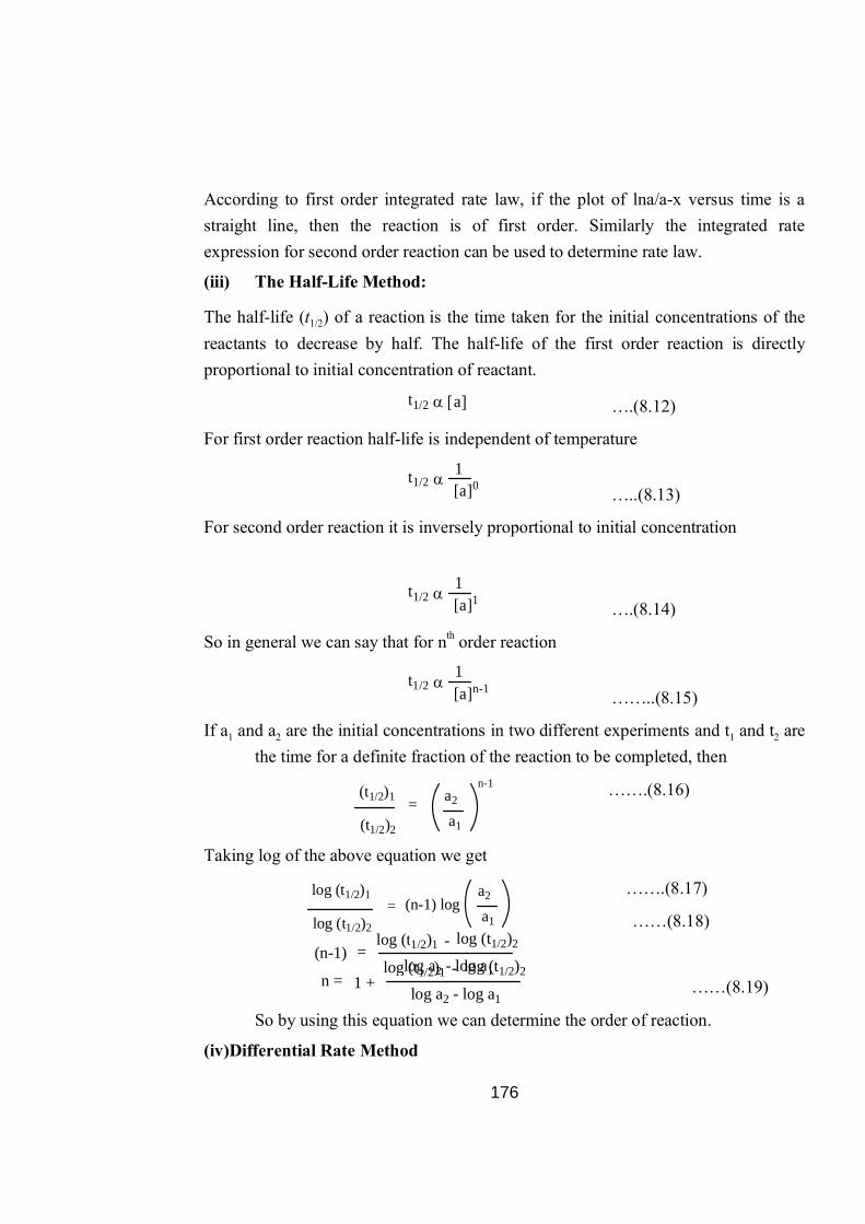
176

According to first order integrated rate law, if the plot of lna/a-x versus time is a straight line, then the reaction is of first order. Similarly the integrated rate expression for second order reaction can be used to determine rate law.

(iii) The Half-Life Method:

The half-life (t1/2) of a reaction is the time taken for the initial concentrations of the reactants to decrease by half. The half-life of the first order reaction is directly proportional to initial concentration of reactant.

t1/2 a ….(8.12)

For first order reaction half-life is independent of temperature

t1/2

1[a]0 …..(8.13)

For second order reaction it is inversely proportional to initial concentration

t1/2

1[a]1 ….(8.14)

So in general we can say that for nth order reaction

t1/2

1[a]n-1 ……..(8.15)

If a1 and a2 are the initial concentrations in two different experiments and t1 and t2 are the time for a definite fraction of the reaction to be completed, then

…….(8.16)

Taking log of the above equation we get

…….(8.17)

……(8.18)

……(8.19)

So by using this equation we can determine the order of reaction.

(iv)Differential Rate Method

(t1/2)1

(t1/2)2

= a2

a1

n-1

log (t1/2)1

log (t1/2)2

a2

a1= (n-1) log

(n-1) =log (t1/2)1 log (t1/2)2-

log a2 - log a1n = 1 +

log (t1/2)1 log (t1/2)2-log a2 - log a1

177

This method was given by Van’t Hoff, according to this method the rate of nth order reaction is:

r = knCn …….(8.20)

Taking log on both side of the equation

ln r = lnkn+ n ln C ……..(8.21)

For two different concentrations C1 and C2of the reactants, we have

ln r1 = lnkn + n ln C1 ………..(8.22)

ln r2 = lnkn + n ln C2 ………..(8.23)

Subtracting equation (8.23) from (8.22)

ln (r1-r2) = n (ln C1- ln C2) ……..(8.24)

n = ln (r1-r2)/(ln C1- ln C2) ………(8.25)

From this equation by putting the values of r1 and r2 at two different concentrations C1 and C2 respectively, we can calculate the order of reaction.

8.5 Temperature Dependence of Reaction Rate

Temperature has a marked effect on the rate of reaction. For most of the reactions, the rate increases with increasing temperature. For every 10°C rise in temperature, the rate of reaction becomes nearly double or triple. The ratio of the rate constants of a reaction at two temperatures differing by 10°C is known as temperature coefficient of the reaction. The temperatures usually selected for this purpose are 25°C and 35°C. Thus

= ≈to 3 ……(8.26) Temperature coefficient

The value of temperature coefficient for most of the reactions is 2 and for some reactions it may be 3. For example value of temperature coefficient for dissociation of H2O2 is 1.7 and for the reaction between CH3I and C2H5ONa, it is 2.9.

k(t+10)kt

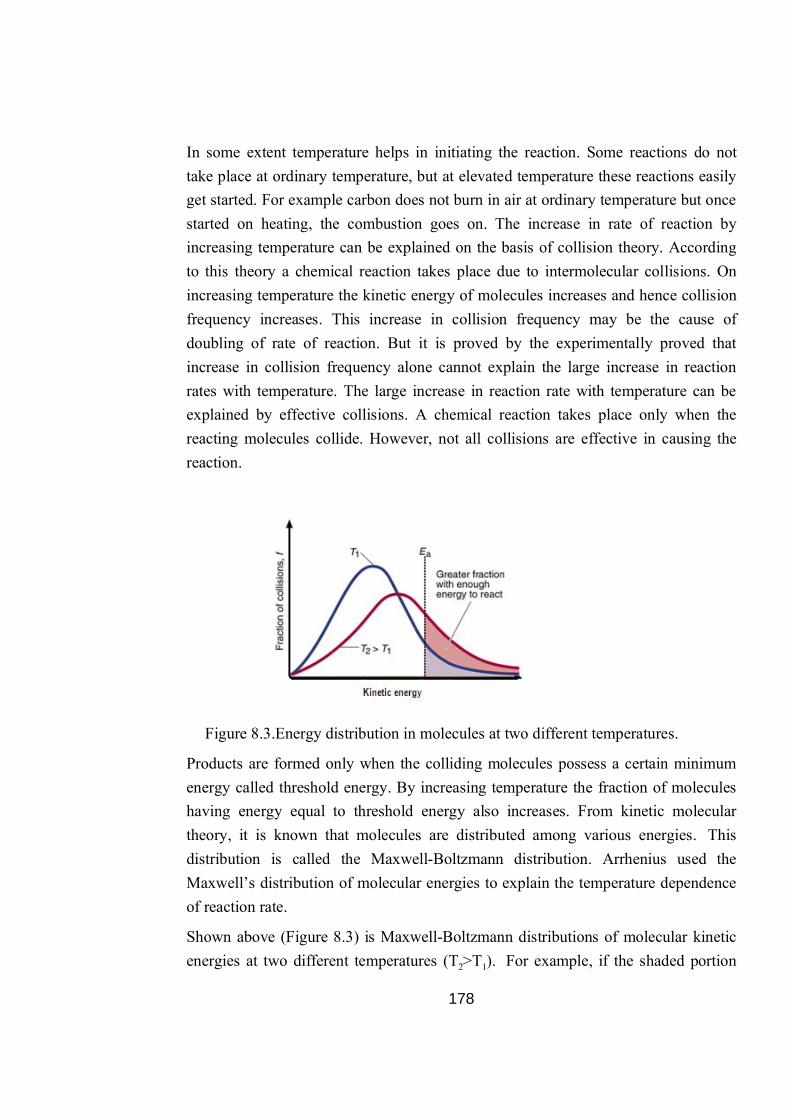
178

In some extent temperature helps in initiating the reaction. Some reactions do not take place at ordinary temperature, but at elevated temperature these reactions easily get started. For example carbon does not burn in air at ordinary temperature but once started on heating, the combustion goes on. The increase in rate of reaction by increasing temperature can be explained on the basis of collision theory. According to this theory a chemical reaction takes place due to intermolecular collisions. On increasing temperature the kinetic energy of molecules increases and hence collision frequency increases. This increase in collision frequency may be the cause of doubling of rate of reaction. But it is proved by the experimentally proved that increase in collision frequency alone cannot explain the large increase in reaction rates with temperature. The large increase in reaction rate with temperature can be explained by effective collisions. A chemical reaction takes place only when the reacting molecules collide. However, not all collisions are effective in causing the reaction.

Figure 8.3.Energy distribution in molecules at two different temperatures.

Products are formed only when the colliding molecules possess a certain minimum energy called threshold energy. By increasing temperature the fraction of molecules having energy equal to threshold energy also increases. From kinetic molecular theory, it is known that molecules are distributed among various energies. This distribution is called the Maxwell-Boltzmann distribution. Arrhenius used the Maxwell’s distribution of molecular energies to explain the temperature dependence of reaction rate.

Shown above (Figure 8.3) is Maxwell-Boltzmann distributions of molecular kinetic energies at two different temperatures (T2>T1). For example, if the shaded portion

179

corresponds to energies greater than or equal to the energy of activation, the areas under the curve tells us the fraction of molecules that possesses energies higher or equal to the energy of activation. A small temperature change, T1 to T2 degrees Celsius, for example, leads to a large effect on the fraction of molecules having enough kinetic energy to react. This clearly shows that the number of molecules having energy equal to or greater than the threshold energy becomes nearly double even with a small increase of temperatures from T1to T2. Thus the rate of reaction which consequently depends on number of effective collisions becomes almost double with small increase in temperature.

The Arrhenius Equation

The dependence of the rate constant of a reaction on temperature can be expressed by the following equation, known as the Arrhenius equation:

k = A.e-Ea/RT ………..(8.27)

whereEa is the activation energy of the reaction (in kJ/mol), R the gas constant (8.314 J/K mol), T the absolute temperature. The quantity A represents the collision frequency and is called the frequency factor. It can be treated as a constant for a given reacting system over a fairly wide temperature range. Equation (8.27) shows that the rate constant is directly proportional to A and, therefore, to the collision frequency. In addition, because of the minus sign associated with the exponent Ea/RT, the rate constant decreases with increasing activation energy and increases with increasing temperature. This equation can be expressed in a more useful form by taking the natural logarithm both side:

ln k = lnA.e-Ea/RT ……….(8.28)

ln k = ln A -Ea/RT ……..(8.29)

Equation (29) can be rearranged to a linear equation:

ln k = (-Ea/R)(1/T) + ln A ……..(8.30)

Thus, a plot of ln k versus 1/T gives a straight line whose slope m is equal to 2Ea/R and whose intercept b with the y axis is ln A.

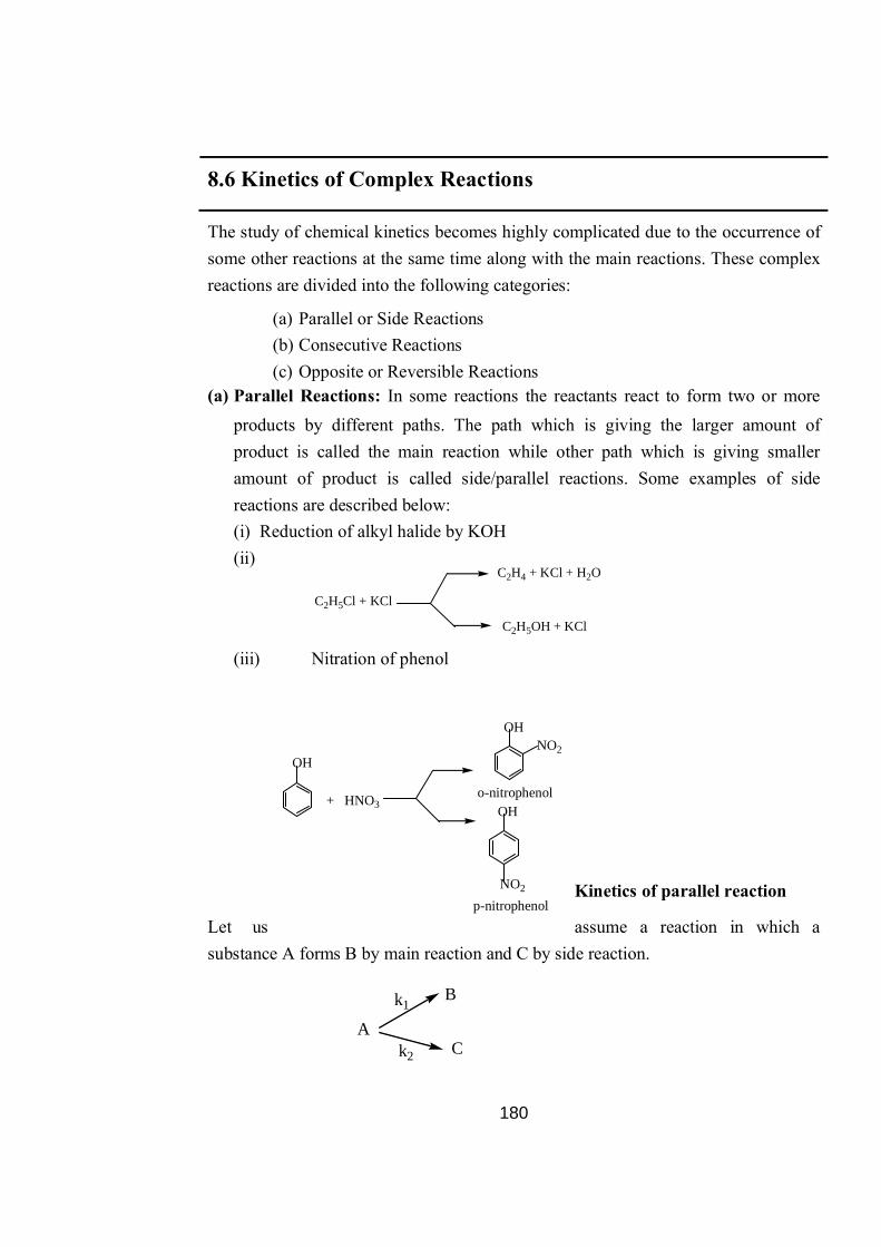
180

8.6 Kinetics of Complex Reactions

The study of chemical kinetics becomes highly complicated due to the occurrence of some other reactions at the same time along with the main reactions. These complex reactions are divided into the following categories:

(a) Parallel or Side Reactions (b) Consecutive Reactions (c) Opposite or Reversible Reactions

(a) Parallel Reactions: In some reactions the reactants react to form two or more products by different paths. The path which is giving the larger amount of product is called the main reaction while other path which is giving smaller amount of product is called side/parallel reactions. Some examples of side reactions are described below: (i) Reduction of alkyl halide by KOH (ii)

(iii) Nitration of phenol

Kinetics of parallel reaction

Let us assume a reaction in which a substance A forms B by main reaction and C by side reaction.

C2H4 + KCl + H2O

C2H5OH + KCl

C2H5Cl + KCl

o-nitrophenol

p-nitrophenol

OH

NO2

NO2

OH

OH

+ HNO3

A

B

C

k1

k2

181

Let k1 and k2be the rate constants for the main and side reactions respectively. If the initial concentration of reactant is “a” moles/L. at time t “x” moles/L decomposed. Now assuming that the reaction is of first order thenrate of main reaction will be

dx/dt = k1 (a-x) ………….(8.31)

And rate of side reaction will be

dx/dt = k2 (a-x) ………(8.32)

So the overall rate of reaction will be

dx/dt = k1 (a-x) + k2 (a-x) ………(8.33)

= (k1 + k2) (a-x) ………(8.34)

By integration and simplification the above equation we will get

[where k1 + k2 = k]

Which is a first order rate equation.

Dividing equation (8.31) by (8.32)

……(8.35)

Hence the ration of products formed is directly proportional to their rate constants at any time.

(b) Reversible or Opposing Reactions: The reactions in which products formed react to produce the original reactants are called Reversible or Opposing Reactions. In such reactions the rate of forward reaction and rate of backward reaction becomes equal, so the net rate of reaction is zero. A well-known example of reversible reaction is hydrolysis of ethyl acetate in the presence of acid.

kln

a-xat = 2.303

CH3COOH + H2O CH3COOH + C2H5OHH+

Rate of formation of B

Rate of formation of C=

k1(a-x)

k2(a-x)

Amount of B formed in time t=

k1

k2Amount of C formed in time t

182

Kinetics of Reversible Reaction: consider a simple reversible reaction in which the forward as well as the reverse reactions are both first order:

Where k1 and k2 are the rate constant of the forward and backward reactions respectively. Let a is the initial concentration of reactant A and after time t, the concentration of A will become (a-x) and that of the product B will be x. so the

Therefore the rate of forward reaction

……..(8.36)

Rate of backward reaction

……..(8.37)

The net rate of reaction is

…….(8.38)

After the establishment of equilibrium, the rates of forward and backward reaction are equal. If the equilibrium concentration of b is xethen,

………(8.39)

………(8.40)

Substituting the above value of k2 in equation (8.38), we have

……..(8.41)

……..(8.42)

……..(8.43)

k2 =k1(a-xe)

xe

dxdt = k1(a-x)

dxdt = k2x

dxdt = k1(a-x) k2x-

k1(a-xe) = k2xe

dxdt = k1(a-x)

k1x(a-xe)xe

-

= k1a -k1xa

xe=

k1axe

(xe-x)

dx(xe-x)

=k1a

xedt

A Bk1

k2

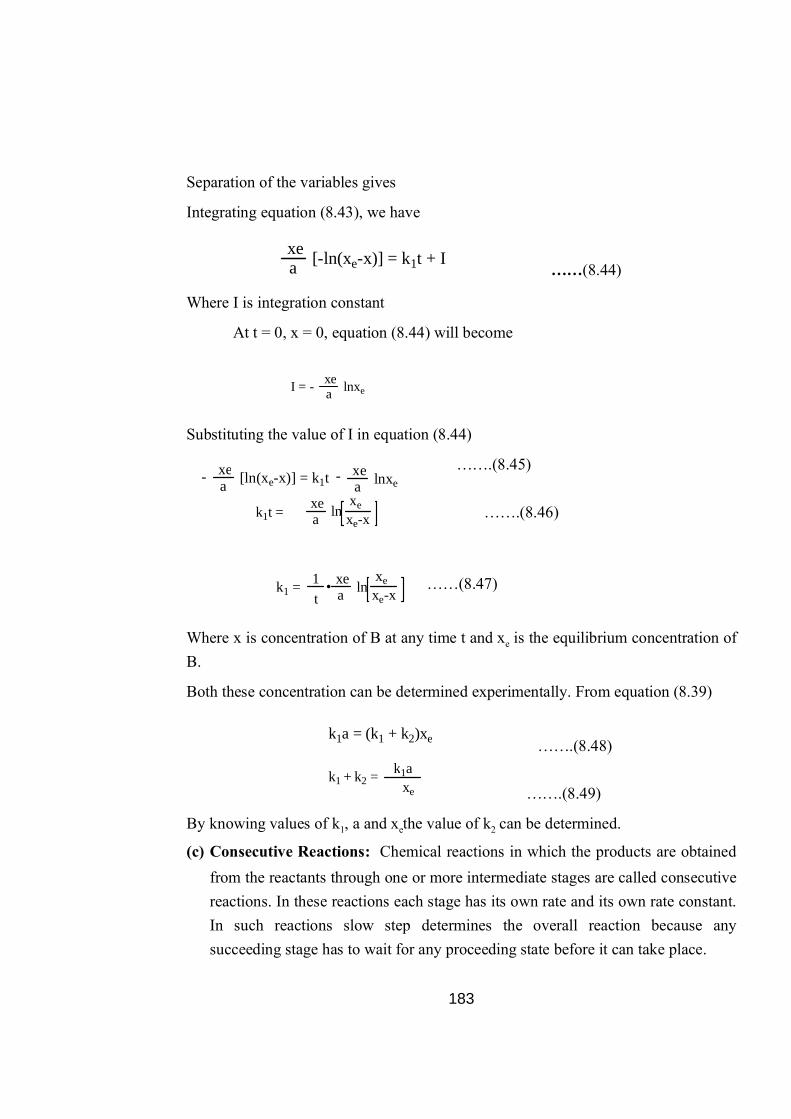
183

Separation of the variables gives

Integrating equation (8.43), we have

……(8.44)

Where I is integration constant

At t = 0, x = 0, equation (8.44) will become

Substituting the value of I in equation (8.44)

…….(8.45)

…….(8.46)

……(8.47)

Where x is concentration of B at any time t and xe is the equilibrium concentration of B.

Both these concentration can be determined experimentally. From equation (8.39)

…….(8.48) …….(8.49)

By knowing values of k1, a and xethe value of k2 can be determined.

(c) Consecutive Reactions: Chemical reactions in which the products are obtained from the reactants through one or more intermediate stages are called consecutive reactions. In these reactions each stage has its own rate and its own rate constant. In such reactions slow step determines the overall reaction because any succeeding stage has to wait for any proceeding state before it can take place.

xea [-ln(xe-x)] = k1t + I

I = - xea lnxe

xea [ln(xe-x)] = k1t- xe

a lnxe-

k1t = xea ln

xexe-x

k1 =1t

xea ln

xexe-x

.

k1 + k2 = k1axe

k1a = (k1 + k2)xe

184

In the above reaction let ‘a’ be the initial concentration of reactant A, same time initial concentration of B and C will be zero. After a time t, let the initial concentration of A decreases to ‘x’ and those of B and C increase to y and z respectively. Then evidently

Then the rate of disappearance of A …..(8.50)

The concentration of B increases in the first step and falls in the second step of the overall reaction.

Rate of formation of B ……(8.51)

Rate of formation of C …….(8.52)

Integrating equation (46) between the limits x = a, t = 0 and x = x and t = t we get

…….(8.53)

…….(8.54)

Substituting the value of x from equation (8.54) in equation (51) we get

…….(8.55)

Integrating equation (55) we have

……..(8.56)

Knowing the value of x and y, the value of z can be calculated. Thus the concentration of A, B and C after different intervals of time can be calculated easily. Similarly by knowing the value of x and y at time t, the value of k1 and k2 can be determined with the help of equation (8.54) and (8.56).

The concentration of A, B and C as the function of time are plotted in Figure 4. It is clearly evident from this figure that concentration of A decreases exponentially while that of C increases gradually. The concentration of B first increases rise to maximum value and then falls asymptotically to zero.

A B Ck1 k2

a = x + y + z

= - dxdt = k1x

= - dydt = k1x - k2y

=dzdt = k2y

k1t = ln ax

x = ae-k1t

dydt

= k1aa-k1t-k

2y

y =k1a

(k2-k1)(e-k

1t - e-k

2t)

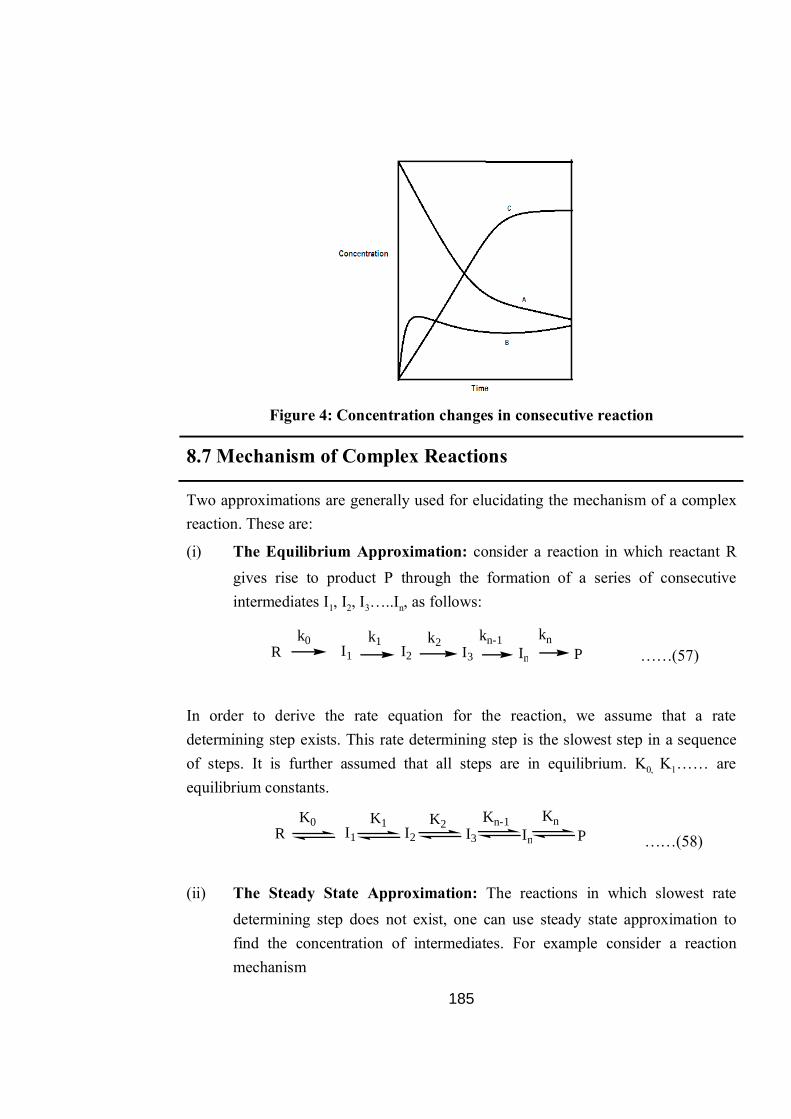
185

Figure 4: Concentration changes in consecutive reaction

8.7 Mechanism of Complex Reactions

Two approximations are generally used for elucidating the mechanism of a complex reaction. These are:

(i) The Equilibrium Approximation: consider a reaction in which reactant R gives rise to product P through the formation of a series of consecutive intermediates I1, I2, I3…..In, as follows:

……(57)

In order to derive the rate equation for the reaction, we assume that a rate determining step exists. This rate determining step is the slowest step in a sequence of steps. It is further assumed that all steps are in equilibrium. K0, K1…… are equilibrium constants.

……(58)

(ii) The Steady State Approximation: The reactions in which slowest rate

determining step does not exist, one can use steady state approximation to find the concentration of intermediates. For example consider a reaction mechanism

R I1 I2 I3 In Pk0 k1 k2 kn-1 kn

R I1 I2 I3 In PK0 K1 K2 Kn-1 Kn

186

……..(59)

According to steady state approximation rate of formation of an intermediate is equal to rate of decomposition of that intermediate so that

d[I1]

dt

d[I2]

dtd[I3]

dt

d[In]

dt= = = = 0

……..(60)

Example:

For the thermal decomposition of ozone to oxygen, the following mechanism has been suggested:

Step 1: ……..(8.61)

Step 2: …….(8.62)

Use steady state approximation and other approximation to account for the observed rate law, viz., r = -k[O3]

2/[O2].

Solution: ozone decomposes in steps 1 and 2 and is formed in the reverse of step 1. Hence

r = d[O3]/dt = -k1[O3] + k-1[O2][O] – k2[O3][O] ……..(8.63)

usings.s.a. for O atom which is an intermediate, we have

d[O]/dt = k1[O3] - k-1[O2][O] – k2[O3][O] = 0 ……..(8.64) k1[O3] = {k-1[O2] + k2[O3]}[O] ………(8.65)

………(8.66)

……..(8.67)

O3 + O 2O2k2

O3 O2 O+k1

k-1

k1[O3]

k-1[O2] + k2[O3][O] =

r = -k1[O] +k1k-1[O3]

k-1[O2] + k2[O3]

[O2] k1k2[O3]2

k-1[O2] + k2[O3]-

R I1 I2 I3 In Pk0 k1 k2 kn-1 kn

187

Substituting for [O] in the rate expression, we have ………(8.68)

On solving this equation

………(8.69)

Now assume that k-1[O2] >>k2[O3], so the second term can be neglected ……….(8.70)

………(8.71) Where k = 2k1k2/k-1

Example 2: The gaseous decomposition of ozone, 2O3 3O2, obeys the rate law, r = -d[O3]/dt = k[O3]

2/[O2]. Show that the following mechanism is consistent with the above rate law:

(Fast equilibrium step)…….(8.72)

(Slow step) ……..(8.73)

Solution: from the slow rate determining step,

R = -d[O3]/dt = k1[O][O3] ……..(8.74)

From the fast equilibrium step

K = [O2][O]/[O3] or [O] = K[O3]/[O2] ……..(8.75)

Substituting for [O] in the expression for r, we have

r = k1K[O3]2/[O2] = k[O3]

2/[O2] ……..(8.76)

where k = k1K

k-1[O2] + k2[O3]

-k1k-1[O3][O2] k1k2[O3]2- k1k-1[O3][O2]+ k1k2[O3]2-

=

r =2k1k2[O3]2

k-1[O2] + k2[O3]-

r = -k[O3]2

[O2]

r =2k1k2[O3]2

k-1[O2]-

188

8.8 Principle of Pre-Equilibria

Let us consider the reaction and its mechanism as a sequence of reactions A + B C ………(8.77)

A + B Xk1

k2 …….(8.78)

X Ck3 ……..(8.79)

where X is an unstable intermediate of the reaction. The rate of formation of substance C is determined by the kinetic equation

…….(8.80)

Where [X] is the concentration of the unstable intermediate, which mostly cannot be obtained experimentally. If the rate of X decomposition into the product C is much lower than the rate of formation of X and its decomposition into the reactants A and B, i.e. if k3<<k2 and k3<<k1,we may approximate the concentration [X] using the relation

K =[X]

[A][B] ………(8.81)

where K is the equilibrium constant of formation of the intermediate. This relation is a mathematical expression of the assumption of pre-equilibrium. Combining equations (9.80) and (9.81) yields

……..(8.82)

8.2 State true/false

a) Lindemann theory from basis of unimolecular reaction (T/F)

b) In Hinsholwood theory K, is different for all energized moleculers (T/F)

c) In RRK theory rate 22 increases with respect to vibrational energy (T/F)

d[C]

dt= k3[X]

d[C]

dt= k3K[A][B]

189

8.9 Kinetic Analysis of decomposition of N2O5

There are cases where the rate determining step of a mechanism contains an intermediate that does not appear in the overall equation. The experimental rate law can only be written, however, in terms of substances that appear in the overall equation.

Consider the decomposition of dinitrogen pentoxide.

2N2O5(g) 4NO2(g) + O2(g)

This reaction is believed to follow this type of mechanism.

2N2O5 2NO2 + 2NO3(fast, equilibrium)

NO2 + NO3 NO + NO2 + O2(slow)

NO3 + NO2 NO2(fast)

It has been determined experimentally that the rate law is:

Rate = k[N2O5]

Let's show that the mechanism outlined above is consistent with the observed rate law. From the last section, we saw that the rate determining step (Step 2 in this case) generally outlines the rate law of the overall equation by which in this case would be:

Rate = k2[NO2][NO3] (Rate law for the rate determining step)

But, as mentioned before, the experimental rate law can only be written in terms of substances contained in the overall equation and cannot contain reaction intermediates. So, it is necessary to re-express the equation eliminating [NO3].

Looking at the first step, we see that it is fast and reversible. The rate of the forward decomposition is defined by the rate law.

Rate = k1[N2O5]

and the rate of the reverse reaction (the formation of N2O5 from NO2 and NO3) is defined as

Rate = k-1[NO2][NO3]

at the beginning of the reaction there is no NO2 or NO3 , but as they begin to form, the reverse reaction begins to pick up speed until finally, an equilibrium is established where the forward and reverse reactions occur at the same rate. Because

190

this first elementary reaction is much faster than the second step, this equilibrium is reached before any significant reaction by the second step occurs. Since at equilibrium, the forward and reverse rates are equal for the first step, we can write:

k1[N2O5] = k-1[NO3][NO2] or, [NO3] =k1[N2O5]/ k-1[NO2]

Substituting this expression into the rate law for the rate determining step, we get

Rate = k2[NO2][NO3]

= k1k2[NO2][N2O5]/ k-1[NO2]

Rate = "k"[N2O5]

So, if we identify k2k1/k-1 as "k", we've reproduced the experimental rate law.

8.10 Unimolecular Reactions

Unimolecular reactions are in principale the simplest type of gas-phase chemical reaction. These reactions are fundamentally important to understand the products observed from activated molecules.

It is very easy to understand a bimolecular reaction on the basis of collision theory. But in a unimolecular reaction

A B The molecule A acquires the necessary activation energy by colliding with another molecule, and then reaction should obey second order kinetics, not first order kinetics which is usually observed in several unimolecular gaseous reactions. A satisfactory theory for these reactions was provided by F.A. Lindemann in 1922.

8.10.1 The LindemannTheory

Lindemann’s theory forms the basis for all modern theories of unimolecular reactions, it was published almost simultaneously by Lindemann (1922) and Christiansen (PhD, 1921): by collision a fraction of molecules becomes energized and gain a critical energy quantity E°. The rate depends on the number of bimolecular collisions and is calculated from the simple collision theory (independent of energy content, Boltzmann distribution):

A + M A* + M (k 1) …..(9.83)

energized molecules are de-energized by collision, the rate is equated to the collision number only (every collision leads to de-energization, pre-exponential term Z):

191

A* + M A + M (k -1) …….(9.84)

there is a time-lag in the unimolecular dissociation process which occurs with a rate constant also independent of the energy content:

A* B + C (k 2) ……(9.85)

the consequences of Lindemann theory are revealed when considering the concentration of energized molecules as constant in the course of the reaction (steady-state approximation) leading to the following expression of the overall rate of reaction:

….(9.86)

At high pressures we find the expected, and experimentally observed, unimolecular process

……..(87)

And at low pressures the reaction rate is then better described by a second order reaction:

…….(9.88)

This theory correctly predicts the rate constant fall-off at low pressures, but the values calculated are far from experimental results (early experimental tests were performed but it is now known that the examples chosen are not unimolecular processes.

We can calculate the pressure at which the rate constant reaches half of its high pressure value (transition pressure):

21

122 k[M]k

[M][A]kk[A*]kv

1

122

k

[A]kk[A*]kv

21[M] kk

[M]12 kk

[A][M]k[A*]kv 12

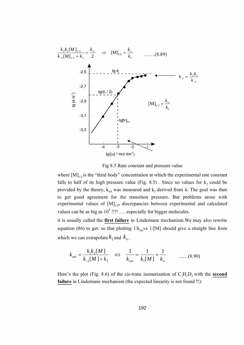
192

…….(8.89)

Fig 8.5 Rate constant and pressure value

where [M]1/2 is the “third body” concentration at which the experimental rate constant falls to half of its high pressure value (Fig. 8.5) . Since no values for k2 could be provided by the theory, kinf was measured and k2 derived from it. The goal was then to get good agreement for the transition pressure. But problems arose with experimental values of [M]1/2, discrepancies between experimental and calculated values can be as big as 108 !!!! …. especially for bigger molecules.

it is usually called the first failure in Lindemann mechanism.We may also rewrite equation (86) to get: so that plotting 1/kunivs 1/[M] should give a straight line from

which we can extrapolate 1k and k .

……(8.90)

Here’s the plot (Fig. 8.6) of the cis-trans isomerization of C2H2D2 with the second failure in Lindemann mechanism (the expected linearity is not found !!):

M

M

12/1[M]

kk

1

12k

k

kk

kMkkkMk

Mkkkuni

uni1

][11

][][

121

21

11/2[M]

kk

2]

22/11

2/112 kk[M]k

[Mkk

193

Fig. 8.6 Cis trans isomelization of C2H2D

by considering the activation energy to be constant, and the collision frequency to be the same in all steps, we can modify the following equation:

………(8.91)

to obtain: Ak2 of the order of a frequency (1013s-1), which is actually contradictory with the time-lag concept introduced to consider the unimolecular step. This is what made Hinshelwood try to modify this theory and especially the expression of the activation rate to account for a longer lifetime of the energized molecule (~1/k2) depending on the number of degrees of freedom (as said previously k2 was not expected to be calculated but inferred from experimental data and especially the success of the theoretical description of the activation step).

Lindemann Shortcomings:

1. The reaction occurs in two steps, a bimolecular activation step and a unimolecular dissociation step.

2. All the rate constants are independent of the internal energy of the molecules. 3. The rate of energization is calculated on the basis of SCT. 4. The rate of de-energization is simply the collision frequency (strong

collision). 5. The unimolecular step is said to be rate determining at high pressure and a

fast step at low pressure.

There are evident two failures:

1

12 k

kkk

194

1. The fall-off critical region is not well-described (discrepancies between theoretical data and experimental data diverge with molecules getting bigger).

2. The linear extrapolation of inverse plot expected is not found experimentally (low pressure description not correct, modification of bimolecular step description).

8.10.2 The Hinshelwood Theory

The first difficulty with the Lindemann treatment that the first order rates are maintained down to lower concentrations than the theory appeared to permit, was overcome by Hinshelwood’s suggestions. According to Hinshelwood the expression z1.e

-Ea/RT applied only if the energy is distributed among two degrees of freedom. Hinshelwood stated that If we start with statistical mechanics, the fraction of molecules containing certain energy between E and E+dE in a single degree of freedom is given by a Boltzmann distribution:

……(8.92)

The total fraction must be 1

……..(8.93)

This gives a=1/kT

……….(8.94)

If we now consider multiple degreis of freedom (s) and define the distributed energy such that the amount in degree 1 is between E1and E1+dE1, energy in degree 2 is between E2and E2+dE2, etc.

……(8.95)

195

Integrating, with the restriction that the sum of the individual energies must be less than or equal to the total E gives:

…..(8.96)

Differentiation of this gives the range of energies between E and E+dE:

….(8.97)

In order to get the rate ratio, this must be integrated between the threshold activation energy for conversion into products and infinity.

……..(8.98)

Solving this integral under certain conditions gives the approximate solution:

……..(8.99)

Strong Collision Approximation: Assuming the energy of the molecule is completely randomized according to the Boltzmann distribution at every collision, the activation rate is proportional to the Boltzmann distribution

……..(8.100)

This differs from the simple collision theory by a factor which takes into account the number of involved harmonic oscillators.

Hinshelwood Improvements/Shortcomings

a) The Hinshelwood model improves upon the Lindemann model by taking into account the degrees of freedom of the reactant.

196

b) However, Hinshelwood has only addressed the problem associated with the energy of activation (the k1process), there exist two additional problems with the k2process.

i) k2 is assumed to be the same for all energized molecules, regardless of there degree of activation

ii) There is only a dependence of activation on the number of frequencies, but there is no dependence of dissociation on the actual specific frequency of the mode of interest.

8.10.3 RRK Theory

Rice and Ramsperger (1927), and later but independently Kassel who introduced at the same time a quantum formulation of the theory (1928), recognized that the rate of the unimolecular step should depend on the vibrational energy of the energized molecule as well. For that purpose, they introduced the idea that a minimum of energy must be localized in specific modes of molecular motion in order for the dissociation to take place, and that the newly calculated rate constant must be proportional to that probability. They did not explicitly mention an activated complex intermediate (TST did not exist at that time!!! this theory appeared during the 30’s) but instead considered the energy localization process to compute the rate constant.

Both of them kept the Hinshelwood-Lindemann theory in its state and modified the expression of the unimolecular step to account for their new idea. They started by considering that energy can flow freely among the different oscillators (which is a rather good approximation as long as the energy involved is big enough compare to the number of oscillators, they can thus be considered as behaving non linearly and being strongly coupled to each other, the strong coupling speeding up the process of transfer, but the oscillators are not harmonic any more …), then Kassel (in its quantum calculations) computed the number of ways to distribute )( m quanta over the s oscillators (since m quanta will be located on the critical oscillator) to get (the quantum calculation is much easier than the classical one, Kassel demonstration will therefore be presented here):

……..(8.101)


)!1()!()!1(

smsm

197

………(8.102)

Considering the classical limit which consists in having a very large number of quanta compare to the number of oscillators, Kassel got:


……(8.103)

whereE0 is the activation energy. E the overall vibrational energy of the molecule, A is a constant, which seems to be an ad hoc term, but is actually the pre-exponential term in the Arrhenius expression when we extrapolate the expression for high pressures. and the overall rate constant is therefore given by (considering the energy dependence of k1 derived in Hinshelwood’s theory):

……(8.104)


The following plot shows how the rate k2 increases with respect to vibrational energy with the number of oscillators available as a parameter (s = 1 corresponds to the case described by Hinshelwood).

1

1

s

mmP

10

2 1)(

s

EEAEk

sms

1)()!(

)!1(

smmsm

)1(

)!1(!

s

s

)!1()!()!1(!

sm

smPm

0

][)(1

/)()(

1

2

112

Euni

MkEk

kdEEEdkEkk

198

which is actually exactly what we need to have a better description at low pressure !!! (low energized molecules will have lower dissociation rate). It should be explained here that the expression derived was initially derived by R and R by considering only classical case all along the calculation. The initial expression given here of the probability P was derived in Kassel’s quantum calculations, which were shown to give the same result as RR in the classical limit ( and m much bigger than s).We will not develop Kassel quantum theory here (it is just a discrete summation of the expression of k2(E) before doing classical limit study), since it was not widely used despite his much better description than classical RRK of the fall-off.

Although Kassel’s theory was giving better agreement to experiments,gross approximations were made (all equivalent classical harmonic oscillators) leading to results for which the number of oscillators couldn’t be predicted a priori (as in Hinshelwood theory).

RRK Improvements/Shortcomings

a) Gave a more accurate picture because the reaction rate had an internal energy dependence.

b) However, the statistical concept of coupled oscillators is vague and not clearly

identifiable with normal modes (which is why the # effective oscillators ≠ # d.o.f.).

c) RRK also attempts to incorporate the magnitude of the specific frequency of the critical oscillator

i) k‡ is the first-order frequency factor for the reaction.

199

ii) For certain molecules this is on the order of average vibrational frequencies, meaning a complete redistribution of energy on every vibration.

iii) However, other reactions have frequency factors higher by several orders of magnitude, which is unexplained by this theory.

8.10.4 RRKM Theory

The RRK theory was an important development in the treatment of unimolecular reactions, but gross approximations were made at that time due to a lack of computational methods (actually no computers were available !!). Marcus, with Rice’s help, developed the now called RRKM theory in 1952. Its main new features with respect to RRK are as follows:

1. The energization rate constant k1 is evaluated as a function of energy by quantum-statistical mechanical treatment.

2. It considers explicitly the concept of Transition State in the unimolecular process as an intermediate step (and converges to ART at the high pressure limit) and deals with the real frequencies of the energized molecule as well as of the TS, and treats explicitly the rotational degrees of freedom in the course of the dissociation.




(i) Fixed energy consists in ZPE and overall translational energy, they are of no interests in the following description.

(ii) The remaining energy, the non-fixed one is assumed to be involved completely in redistribution during the reaction (IVR hypothesis discussed in the next chapter), even if Marcus dealt with non-active modes in his original

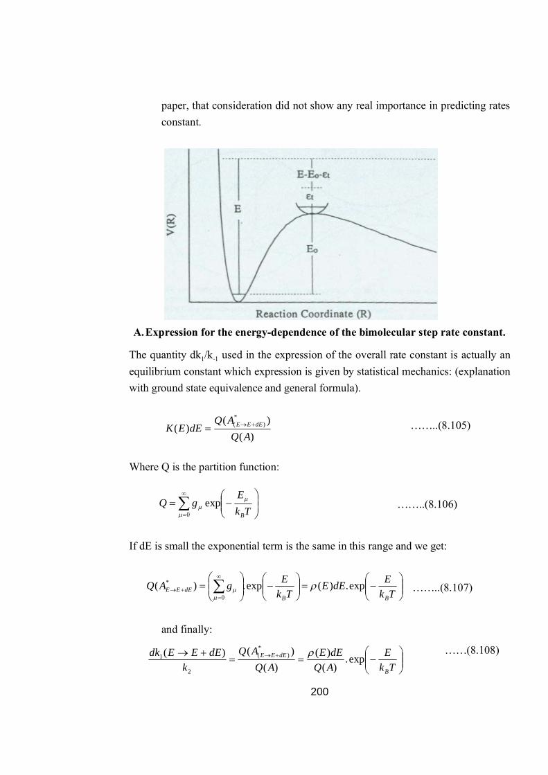
200

paper, that consideration did not show any real importance in predicting rates constant.

A. Expression for the energy-dependence of the bimolecular step rate constant.

The quantity dk1/k-1 used in the expression of the overall rate constant is actually an equilibrium constant which expression is given by statistical mechanics: (explanation with ground state equivalence and general formula).

……..(8.105)

Where Q is the partition function:

……..(8.106)

If dE is small the exponential term is the same in this range and we get:

……..(8.107)

and finally:

……(8.108)

0exp

Tk

EgQ

B

)()(

)(*

)(

AQAQ

dEEK dEEE

Tk

EdEETk

EgAQBB

dEEE exp.)(exp.)(0

*

TkE

AQdEE

AQAQ

kdEEEdk

B

dEEE exp.)(

)()(

)()( *)(

2

1

201

Which is in fact the quantum Boltzmann distribution giving the thermal equilibrium proportion of molecules in the given energy range.

B. Expression for the energy dependence of the dissociation step.


we get: ][][

21)( *2 A

AkEk

……..(9.109)


……….(9.110)

with x the translational energy of the molecule at the top of the barrier, m its mass, and the length of the “box”.

Considering again the two species to be at thermal equilibrium, the ratio of their concentrations is then expressed as the ratio of their partition function (they have the same ground state energy), both these species have the total energy in the same range

dEEE and the ratio of their partition function reduces to the ratio of the sum of the degeneracies, which at the energy of interest, chemical energies, can be approximated by the ratio of their density of states:

…….(9.111)


By using the expression of the number of states given in our lecture on TST, and by considering all the calculated expression, we get the for the activation rate constant:

………(9.112)

2/1

2

2

mxk

)()()(

][][

*** ExNEP

AA

eq

E

E

EPEh

Ek0

'**2

'

)()(

1)(

202


We did not actually consider the effect of adiabatic rotations in these calculations (explanation here of adiabatic rotations), and to converge to ART at the high pressure limit, we should take them into account. This can be simply done by multiplying the above expression by the ratio of the rotational partition functions (this idea has only limited validity at low pressure where another procedure is required).

Another point has been omitted, is the problem of multiple reaction paths. The example of dissociation of H2O leads to two equivalent paths, and to account for that we should include another factor called statistical factor or reaction path degeneracy L# (short explanation here).


…..(8.113)


which leads to the same results as in ART !!!

2. Major approximations in RRKM.

A. Intramolecular Vibrational Relaxation:


As mentioned previously, Marcus made provision for some of the degrees of freedom to be completely inactive and which could therefore not participate to the dissociation process. This energy can however be redistributed randomly between these modes and affects the density of states of the energized molecule as well as the activation rate constant.There is little evidence that energy is rapidly redistributed between all vibrational modes involved within a time not greater than 10-11 s.This

E

E

EPEhQ

QLEk0

'**

1

12

'

)()(

1)(

203

assumption may reach his limits when considering e.g. huge molecules (fragmentation of polymers or biomolecules), or very low energy barrier (isomerization of rather big enough molecules). It is usually called non-ergodic process (no time for energy to explore the complete phase space), but you may find this term in publications whenever there is something not understood.

B. Strong collisions assumption:

This assumption means that relatively large amounts of energy are transferred in molecular collisions (>>kT). RRKM assumes then the energization step to be single-step on contrary to ladder-climbing processes. This assumption also assumes that the molecule after collision is in a state completely independent as the one before, no dynamical details of the collision are thus necessary within that description.

A more detailed study of energization step can be done involving accurate description of the dynamics of collision, and it seems relatively important for small molecules. However it was shown that multiplying the de-energization rate constant

by a constant λ less than unity, leading to shift of the curve log(kuni) vs. log(p) by log

λis sufficient to give rather good agreement with experimental data.

C. The equilibrium hypothesis:

In the unimolecular step it was assumed as in ART that the TS is crossed as if there would be equilibrium between energized and activated molecules (SSA as if no net reaction is occurring, total equilibrium of reverse reaction).


D. Continuous distribution function of state density:

The approximation of continuous density of states for the activated complex can be cumbersome, since most of the energy available is fixed to overcome the barrier and a part of it stored in the translational motion. This approximation holds very well for highly excited molecules (density of states becomes a continuous function of energy) but can become problematic when the energies involved are just above chemical energies.

204

An example is given for cyclopropane with excitation energy E*=70kcal/mol and E#=5kcal/mol, A* has 4.109 vibrational quantum states/kcal and A# has only 102.a continuous approximation of density of states is thus less valid for activated complex.

8.11Summary

1. The rate of a chemical reaction is the change in the concentration of reactants or products over time. The rate is not constant, but varies continuously as concentrations change.

2. The rate law expresses the relationship of the rate of a reaction to the rate constant and the concentrations of the reactants raised to appropriate powers. The rate constant k for a given reaction changes only with temperature.

3. Reaction order is the power to which the concentration of a given reactant is raised in the rate law. Overall reaction order is the sum of the powers to which reactant concentrations are raised in the rate law. The rate law and the reaction order cannot be determined from the stoichiometry of the overall equation for a reaction; they must be determined by experiment. For a zero-order reaction, the reaction rate is equal to the rate constant.

4. The half-life of a reaction (the time it takes for the concentration of a reactant to decrease by one-half) can be used to determine the rate constant of a first order reaction.

5. In terms of collision theory, a reaction occurs when molecules collide with sufficient energy, called the activation energy, to break the bonds and initiate the reaction. The rate constant and the activation energy are related by the Arrhenius equation.

6. The overall balanced equation for a reaction may be the sum of a series of simple reactions, called elementary steps. The complete series of elementary steps for a reaction is the reaction mechanism.

7. If one step in a reaction mechanism is much slower than all other steps, it is the rate-determining step.

8.12 Glossory

Rate of reaction : The change in concentration of reactants or products.

205

Rate low : equation that tolls how the reaction rate depends on the concentsotion

of rate of chemical species involve.

Order of reaction : Number of molecules whose concentration changes during

reaction.

Paralled reaction : Reactions reart to form two or more products bydifferent path.

Consecutive reation : Products are abtened from the reactants through one or

more intermediate stages. Answer to say assessment questions

8.1 a) increases b) mat-1 sec-1 c) straight line d) independent

8.2 a) T b) F c) T


1 Explain the terms rate constant and order of reaction?

2 State and explain the effect of temperature on reaction rate. How energy of activation is determined by Arrhenius equation?

3 Discuss the kinetics of reversible and chain reactions.

4 Describe the Lindemann theory of unimolecular reaction.

5 Using the Rice-Herzfeld mechanism for the reaction H2 + Br2 HBr, employing steady state approximation for [H] and [Br], derive the rate law expression for the formation of HBr.

6 Consider the following mechanism for the unimolecular decomposition of a molecule A in the presence of species M:

A + M A* + M

A* + M A + M

A* P

k1

k-1

k2

(Activation)

(Deactivation)

(Decomposition) Using steady state approximation, derive the rate law for the formation of product.

7 The rate law for decomposition of gaseous N2O5,

206

is observed to be = -d[N2O5]/dt = k[[N2O5]

A reaction mechanism which has been suggested is

Show that the mechanism is consistent with the rate law.

8 Use the Arrhenius equation to show why the rate constant of a reaction (a) decreases with increasing activation energy and (b) increases with increasing temperature.

9 the rate law expression for the reaction

is r = k[NO][O2]. Suggest a possible mechanism consistent with rate law.

10 The rate constants for the decomposition of acetaldehyde

CH3CHO(g) CH4(g) + CO(g)

were measured at fi ve different temperatures. The data are shown in the table. Plot ln k versus 1/T, and determine the activation energy (in kJ/mol) for the reaction. Note that the reaction is “3/2” order in CH3CHO, so k has the units of 1/M1/2

K [1/M1/2.s) T (K)

0.011 700

0.035 730

0.105 760

0.343 790

0.789 810

NO2 + NO3NO2 + NO + O2

NO + NO32NO2

N2O5 NO2 + NO3K

k1

k2

N2O5 2NO2 + 1/2O2

2NO + O2 2NO2

207

Q.11 For the nth order reaction, show that:

n = ln (r1-r2)/(ln C1- ln C2)

8.14 Suggested Readings

1. S. Glasstone- Text book of Physical Chemistry. 2. Physical Chemistry – G. M. Barrow, Tata-McGraw Hill, Vth edition, 2003. 3. R. Stephen Berry, Stuart A. Rice and John Ross, Physical Chemistry 2nd edn,

Oxford Univ. Press, New York, 2000. 4. J.I. Steinfeld, J.S. Francisco and W.L. Hase, Chemical Kinetics and Dynamics,

2nd edn, Prentice Hall, New Jersey, 1999. 5. Atkins, P. W. & Paula, J. de Atkin’s Physical Chemistry 8th Ed., Oxford

University Press, (2006). 6. D. A. Mc Quarrie and D. Simon, Physical chemistry, A Molecular Approach ,Viva

Books Pvt. Ltd, New Delhi, 2003. 7. B.R. Puri, L.R. Sharma, M.S. Pathania, Principles of Physical Chemistry, Vishal

Publishing Coporation, Jalandhar, 2012.

208

Unit – 9 : Enzyme Catalysis Structure of Unit

9.0 Objectives

9.1 Introduction

9.2 Types of Catalysis

9.3 Characteristics of Catalytic Reactions

9.4 Catalytic Promoters and Poisons

9.5 Auto-Catalysisa

9.6 Negative Catalysis

9.7 Enzyme Catalysis

9.8 Chain Reactions

9.9 Branching Chain- Explosive Reactions

9.10 Decomposition of Water

9.11 Summary

9.12 Glossary


9.12 Multiple Choice Questions



209

By the end of this chapter you should be able to:

Relate the purpose and importance of enzymes as catalysts.

Understand the thermodynamics of an enzymatic catalyzed reaction.

Be able to recognize the basic reaction classification of various enzymes.

Recognize the type of catalysis for each of the enzymes studied.

Describe how enzymes are specific in both their substrate and reactant.

Know the Michaelis-Menten mechanism of enzymes catalysis.

Understand the mechanism of chain reactions.

Understand the type of explosion reactions.

Know the process of decomposition of water.

9.1 Introduction

Berzelius (1836) realized that there are substances which increase the rate of a reaction without themselves being consumed. He believed that the function of such a substance was to loosen the bonds which hold the atoms in the reacting molecules together. Thus he coined the term Catalysis (Greek kata = wholly, lein = to loosen). There is no doubt that usually a catalyst accelerates a reaction. But a number of cases are now known where the catalyst definitely retards (slows down) the rate of reaction. A catalyst is defined as a substance which alters the rate of a chemical reaction, itself remaining chemically unchanged at the end of the reaction. The process is called Catalysis. As evident from the above definition, a catalyst may increase or decrease the rate of a reaction. A catalyst which enhances the rate of a reaction is called a Positive catalyst. A catalyst which retards the rate of a reaction is called a Negative catalyst and the process Negative catalysis.

9.2 Types of Catalysis

There are two main types of catalysis:

(a) Homogeneous catalysis

(b) Heterogeneous catalysis

9.0 Objectives

210

(a) Homogeneous Catalysis

In homogeneous catalysis, the catalyst is in the same phase as the reactants and is evenly distributed throughout. This type of catalysis can occur in gas phase or the liquid (solution) phase. For example

(i) oxidation of sulphur dioxide (SO2) to sulphur trioxide (SO3) with nitric oxide (NO) as catalyst,

2SO2(g) + O2(g) + [NO](g)⎯⎯→ 2SO3+ [NO]

Many reactions in solutions are catalysed by acids (H+) and bases (OH–).For example

(i) Hydrolysis of cane sugar in aqueous solution in the presence of mineral acid as catalyst,

C12H22O11(l)+ H2O + H2SO4⎯2

(l)⎯⎯⎯→ C6H12O6 + C6H12O6 + [H2SO4]

(ii) Hydrolysis of an ester in the presence of acid or alkali

CH3COOC2H5(l) + H2O(l) + H+/OH-⎯⎯⎯→ CH3COOH + C2H5OH

(b) Heterogeneous Catalysis

The catalysis in which the catalyst is in a different physical phase from the reactants is termed Heterogeneous catalysis. The most important of such reactions are those in which the reactants are in the gas phase while the catalyst is a solid. The process is also called Contact catalysis since the reaction occurs by contact of reactants with the catalyst surface. In contact catalysis, usually the catalyst is a finely divided metal. This form of catalysis has great industrial importance. Examples of Heterogeneous Catalysis Some examples of heterogeneous catalysis with reactants in the gas, liquid or the solid phase are listed below.

(i) Combination of sulphur dioxide (SO2) and oxygen in the presence of finely divided platinum or vanadium pentoxide, V2O5,

2SO2(g) + O2(g) + [Pt](s)⎯⎯→ 2SO3(g) + [Pt]

(ii) The decomposition of aqueous solutions of hydrogen peroxide (H2O2) is catalysed by manganese dioxide (MnO2) or platinum in colloidal form,

2H2O2(l) + [Pt](s)⎯⎯→ 2H2O + O2 + [Pt]

211

(iii) The decomposition of potassium chlorate (KClO3) is catalysed by manganese dioxide (MnO2).

2KClO3(s) + [MnO2] (s)⎯⎯→ 2KCl + 3O2 + [MnO2]

9.3 Characteristics of Catalytic Reactions

Although there are different types of catalytic reactions, the following features or characteristics are common to most of them.

1. A catalyst remains unchanged in mass and chemical composition at the end of the reaction Qualitative and quantitative analysis show that a catalyst undergoes no change in mass of chemical nature. However, it may undergo a physical change. Thus granular manganese dioxide (MnO2), used as a catalyst in the thermal decomposing of potassium chlorate is left as a fine powder at the end to the reaction.

2. A small quantity of catalyst is generally needed to produce almost unlimited reaction Sometimes a trace of a metal catalyst is required to affect very large amounts of reactants. For example, one ten-millionth of its mass of finely divided platinum is all that is needed to catalyse the decomposition of hydrogen peroxide. On the other hand, there are catalysts which need to be present in relatively large amount to be effective. Thus in Friedel-Crafts reaction,

C6H6 + C2H5Cl + AlCl3⎯⎯→ C6H5C2H5 + HCl

Anhydrous aluminium chloride functions as a catalyst effectively when present to the extent of 30 per cent of the mass of benzene.

3. A catalyst is more effective when finely divided. In heterogeneous catalysis, the solid catalyst is more effective when in a state of fine subdivision than it is used in bulk. Thus a lump of platinum will have much less catalytic activity than colloidal or platinised asbestos. Finely divided nickel is a better catalyst than lumps of solid nickel.

4. A catalyst is specific in its action, while a particular catalyst works for one reaction, it will not necessarily work for another reaction. Different catalysts, moreover, can bring about completely different reactions for the same substance.

212

For example, ethanol gives ethene when passed over hot aluminium oxide, but with hot copper it gives ethanal (CH3CHO).

C2H5OH + Al2O3→ CH2=CH2 + H2O

C2H5OH + Cu → CH3CHO + H2 (Dehydrogenation)

5. A catalyst cannot, in general, initiate a reaction. In most cases a catalyst speeds up a reaction already in progress and does not initiate (or start) the reaction. But there are certain reactions where the reactants do not combine for very long period (perhaps years). For example, a mixture of hydrogen and oxygen, which remains unchanged almost indefinitely at room temperature, can be brought to reaction by the catalyst platinum black in a few seconds.

H2 + O2 room temp. → No reaction

2H2 + O2 Pt black → 2H2O Thus it is now considered that the catalyst can initiate a reaction. According to this view, the reacting molecules (in the absence of catalyst) do not possess minimum kinetic energies for successful collisions. The molecules rebound from collision without reacting at all.

6. A catalyst does not affect the final position of equilibrium, although it shortens the time required to establish the equilibrium It implies that in a reversible reaction the catalyst accelerates the forward and the reverse reactions equally. Thus the ratio of the rates of two opposing reactions i.e., the equilibrium constant, remains unchanged. For example, in the Haber Process for ammonia,

N2 + 3H2 + Fe 2NH3 the reaction is very slow. In the presence of the catalyst, the equilibrium is reached much sooner but the percentage yield remains unchanged. The iron catalyst shortens the time to attain equilibrium but cannot alter the percentage yield.

7. Change of temperature alters the rate of a catalytic reaction as it would do for the same reaction without a catalyst. Some catalysts are, however, physically altered by a rise in temperature and hence their catalytic activity may be decreased. This is particularly true with colloidal solutions like that of platinum, since a rise in the temperature may cause their coagulation. In such a case the rate of reaction increases up to a certain point and then gradually decreases. The rate of reaction is maximum at a particular temperature called the optimum temperature.

213

9.4 Catalytic Promoters and Poisons

The activity of a catalyst can often be increased by addition of a small quantity of a second material. This second substance is either not a catalyst itself for the reaction or it may be a feeble catalyst. A substance which, though itself not a catalyst, promotes the activity of a catalyst is called a promoter. For example Molybdenum (Mo) or aluminium oxide (Al2O3) promotes the activity of iron catalyst in the Haber synthesis for the manufacture of ammonia.

N2 + 3H2 + Fe/Mo 2NH3

In some reactions, mixtures of catalysts are used to obtain the maximum catalytic efficiency. For example, in the synthesis of methanol (CH3OH) from carbon monoxide and hydrogen, a mixture of zinc and chromium oxide is used as a catalyst.

A substance which destroys the activity of the catalyst to accelerate a reaction, is called a poison and the process is called Catalytic poisoning. For example the platinum catalyst used in the oxidation of sulphur dioxide (Contact Process), is poisoned by arsenic oxide (As2O3).

SO2 + O2 + Pt/ As2O3 2SO3

9.5 Autocatalysis

When one of the products of reaction itself acts as a catalyst for that reaction the phenomenon is called Autocatalysis. Autocatalysis is a process during which the products of a reaction catalyze its course. An example of autocatalysis is the oxidation of oxalic acid by permanganate ions in an acidic environment catalyzed by manganous ions.

5 (COOH)2+ 2MnO4− + 6H+ 8H2O + 10CO2 + 2Mn2+

The initial course of the reaction is very slow, but as soon as a certain amount of Mn2+ ions is formed, the rate of reaction increases many times. Catalysis may be homogeneous, in which case the catalyst is in the same phase (gas or liquid) as the reactants (substances participating in the reaction), and heterogeneous, in which case the catalyst is usually in the solid phase and the reactants are either gaseous or liquid.

Examples of Autocatalysis

214

(1) Hydrolysis of an Ester. The hydrolysis of ethyl acetate forms acetic acid (CH3COOH) and ethanol. Of these products, acetic acid acts as a catalyst for the reaction.

CH3COOC2H5 + H2O ⎯⎯→ CH3COOH + C2H5OH (2) Oxidation of Oxalic acid. When oxalic acid is oxidised by acidified potassium

permanganate, manganous sulphate produced during the reaction acts as a catalyst for the reaction.

2KMnO4 + 5H2C2O4 + 3H2SO4⎯⎯→ 2MnSO4+ K2SO4 + 8H2O + 10CO2

9.1 Fill in the blanbks

a) Hydrolysis of a on exter is example of ---------------(auto catalysis/thermal

catalysis)

b) Contlyst remain unchaged in nass and -------------------at the end of

reaction (chemical composition/chemical weight)

c) Reaction occurs by contert of reactants by catalyst surface in

………..(homogenous catalysis/contect catalysis)

d) Catalysis are -----------------in nature (hot specific/specilie)

9.6 Negative Catalysis

When a catalyst reduces the rate of a reaction, it is called a Negative catalyst or Inhibitor. This phenomenon is called Negative catalysis or Inhibition. Negative catalysis is useful to slow down or stop altogether an unwanted reaction.

For example oxidation of CHCl3 in the presence of ethanol forms carbonyl chloride (COCl2) which is a poisonous substance.

4CHCl3+ 3O2+ (C2H5OH) ⎯⎯→ 4COCl2 + 2H2O + 2Cl2

Similarly decomposition of hydrogen peroxide,

2H2O2⎯⎯→ 2H2O + O2

is retarded by the presence of dilute acids or glycerol.

215

Exercise:

1. What are catalytic promoters and poisons? 2. Distinguish between homogeneous and heterogeneous catalysis. 3. What do you understand by positive and negative catalysis. 4. Explain the term Autocatalysis. 5. Why it is necessary to remove arsenic impurity in the manufacturing of SO3 by

contact process. 6. When acidic KMnO4 solution is added to a hot solution of oxalic acid, the colour

is decolorized slowly in the beginning, but after some time it disappears readily why?

9.7 Enzyme Catalysis

Numerous organic reactions are taking place in the body of animals and plants to maintain the life process. These reactions being slow remarkably catalyzed by the organic compounds known as Enzymes. All enzymes have been found to be complex protein molecules. Thus enzymes are protein molecules which act as catalysts to speed up organic reactions in living cells. The catalysis brought about by enzymes is known as Enzyme Catalysis. Each enzyme is produced in a particular living cell to catalyse a reaction occurring in that cell. Many enzymes have been identified and obtained in pure crystalline state from the cells to which they belong. However the first enzyme as prepared by synthesis in the laboratory in 1969.

Examples of Enzyme Catalysis Some common examples of the biochemical reactions catalysed by enzymes are:

(i) Inversion of cane sugar by Invertase present in yeast,

C12H22O11 + invertase⎯⎯⎯⎯⎯→ C6H12O6 + C6H12O6

(ii) Conversion of glucose into ethanol by Zymase present in yeast,

C6H12O6 + zymase⎯⎯⎯⎯→ C2H5OH

(iii) Hydrolysis of urea by Urease present in soya bean,

H2NCONH2 +H ++ Urease ⎯⎯⎯→ 2NH3 + CO

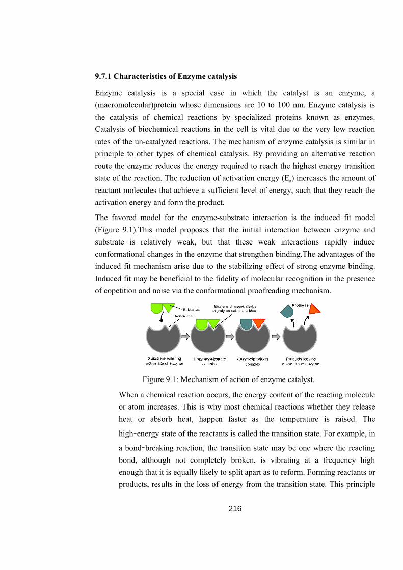
216

9.7.1 Characteristics of Enzyme catalysis

Enzyme catalysis is a special case in which the catalyst is an enzyme, a (macromolecular)protein whose dimensions are 10 to 100 nm. Enzyme catalysis is the catalysis of chemical reactions by specialized proteins known as enzymes. Catalysis of biochemical reactions in the cell is vital due to the very low reaction rates of the un-catalyzed reactions. The mechanism of enzyme catalysis is similar in principle to other types of chemical catalysis. By providing an alternative reaction route the enzyme reduces the energy required to reach the highest energy transition state of the reaction. The reduction of activation energy (Ea) increases the amount of reactant molecules that achieve a sufficient level of energy, such that they reach the activation energy and form the product.

The favored model for the enzyme-substrate interaction is the induced fit model (Figure 9.1).This model proposes that the initial interaction between enzyme and substrate is relatively weak, but that these weak interactions rapidly induce conformational changes in the enzyme that strengthen binding.The advantages of the induced fit mechanism arise due to the stabilizing effect of strong enzyme binding. Induced fit may be beneficial to the fidelity of molecular recognition in the presence of copetition and noise via the conformational proofreading mechanism.

Figure 9.1: Mechanism of action of enzyme catalyst.

When a chemical reaction occurs, the energy content of the reacting molecule or atom increases. This is why most chemical reactions whether they release heat or absorb heat, happen faster as the temperature is raised. The

high‐energy state of the reactants is called the transition state. For example, in

a bond‐breaking reaction, the transition state may be one where the reacting bond, although not completely broken, is vibrating at a frequency high enough that it is equally likely to split apart as to reform. Forming reactants or products, results in the loss of energy from the transition state. This principle

217

is shown in Figure 9.2, where the increased energy of the transition state is represented as a hill or barrier on the energy diagram. Catalysts reduce the height of the barrierforachievingthetransitionstate.

Figure 9.2: Energy diagram for enzyme catalysis.

9.7.2 Enzyme kinetics: the Michaelis-Menten equation

A vast number of reactions in living systems are catalyzed by protein molecules calledenzymes. The lock and key hypothesis of enzyme action (Figure 9.3)supposesthat the enzyme, E, contains a very specific binding site into which fits only the targetsubstrate, S, to form an enzyme-substrate complex, ES, which may undergo unimoleculardecomposition back to E and S, or unimolecular reaction to form product, P, and thererelease of E for further reaction.

Figure 3: Lock and key model for enzyme action.

The general kinetic mechanism parallels that of the Lindemann mechanism underlpinning unimolecular reactions. The overall rate of product formation is equal

218

to k2[ES] and the value of [ES] is evaluated by equating the rates of ES formation and removal under the steady state assumption:

k1[E][S]=k−1[ES]+k2[ES] ….(9.1)

or,

…..(9.2)

If [E]0 is the total concentration of enzyme present then [E]0=[E]+[ES], and substituting for [E] in the expression for [ES] gives:

…..(9.3)

which rearranges to:

…..(9.4)

In enzyme kinetics, the symbol v is often used to denote observed reaction rates:

……(9.5)

By dividing both the numerator and denominator by k1 and defining (k−1+k2)/k1 as KM, the Michaelis constant, the observed rate of reaction simplifies to:

…….(9.6)

This rate law is known as the Michaelis-Menten equation and shows that the rate of enzyme-mediated reaction is first order with respect to enzyme concentration. The overall rate depends on the concentration of substrate. At low substrate concentrations, so the rate of reaction is first order in substrate concentration as well as enzyme concentration:

……(9.7)

When the substrate concentration is sufficiently high that, the overall rate of reaction is zero order in [S]:

v=k2[E]0 ……(9.8)

219

The rate of reaction is independent of substrate concentration under these conditions because at any given time all active sites of the enzymes are filled and increasing the amount of substrate cannot increase the yield of product. The rate determining step is therefore the rate at which the ES complex reacts to form products. These conditions also correspond to the maximum rate of reaction:

vmax=k2[E]0 …….(9.9)

andk2 is often termed the maximum turnover number.

9.7.3 Enzyme kinetics: Lineweaver-Burke plots

The Michaelis-Menten equation can be expressed in a different form by taking the reciprocal of both sides:

………(9.10)

Substituting for the maximum rate of reaction, υmax=k2[E]0, gives

……..(9.11)

Therefore, the reciprocal of reaction rate is directly proportional to the reciprocal of substrate concentration when the total concentration of enzyme is held constant. The graph of 1/v plotted against 1/[S] is a straight line and is known as a Lineweaver-Burke (Figure 9.4).

Figure 9.4: The Lineweaver-Burke plot for enzyme kinetics. The reciprocal of reaction rate, v, is plotted against the reciprocal of substrate concentrations,[S], for experiments using the same total enzyme concentration.

220

9.8 Chain Reactions

A chain reaction occurs when a reaction intermediate generated in one step reacts with another species to generate another reaction intermediate. A chain reaction mechanism typically contains several types of elementary reaction steps including initiation, propagation, branching and termination. Mechanisms containing many branching reactions may lead to explosions.

In many complex reaction systems, the product of one elementary reactions step is the reactant in the next elementary reaction step, and so on. Such systems are called chain reactions and the reactive intermediates responsible for the propagation of the reaction are called chain carriers. Important examples of such processes include combustion reactions in flames, the reactions that contribute to ozone destruction in the upper atmosphere, nuclear fission, or the formation of polymers in solution.

9.8.1 Kinetics of Thermal reaction of H2 and Br2

A typical chain reaction is that between H2 and Br2 to form HBr

H2(g) + Br2(g) →2HBr(g)

For which a five step mechanism has been proposed:

The following reaction scheme explains the complex observed empirical rate law,

..…(9.12)

1) Chain Initiation. The initiation step is the unimolecular dissociation of Br2 to produce the first free radical chain carriers. (Free radicals are reactive species containing unpaired electrons in their valence shells).

Br2 2Br

Br + H2 HBr + H

H + Br2 HBr + Br

H + HBr H2 + Br

2Br Br2

k1

k2

k3

k4

k5

(Chain initiation)

(Chain propagation)

(Chain propagation)

(Chain retardation)

(Chain termination)

d[HBr]

dt= k[H2][Br2]3/2

221

Br2→2Br

Rate=k1[Br2] ……(9.13)

2) Chain Propagation. Propagation reactions convert reactive intermediates from a preceding elementary reaction into another reactive intermediate. The total number of reactive intermediates is unaltered. There are two different propagation reactions in the HBr mechanism:

Br+H2→HBr+H

Rate=k2[Br][H2] ……(9.14)

And

H+Br2→HBr+Br

Rate=k2[H][Br2] ……(9.15)

Although not present in the HBr mechanism, branching reactions are a specific type of propagation reaction in which more chain carriers are produced than are consumed.

3) Chain Retardation. The attack of an H radical on a product HBr molecule formed in a previous propagation step, although still generating another free radical, has the effect of decreasing, or retarding, the overall rate of product formation.

H+HBr→H2+Br

Rate=k3[H][HBr] ……(9.16)

4) Chain Termination. Elementary reactions in which radicals combine to reduce the total number of radicals present are called termination steps.

Br+Br+M→Br2+M

Rate=k4[Br]2 ……..(9.17)

In this association reaction, the third body M represents any species present which removes the energy of the recombination collision between the Br atoms to form the stabilized Br2 molecule. The concentration of M (which is a constant for given reaction conditions) is included in the value of the rate constant k4. Although other chain termination reactions are possible, e.g. recombination of two H radicals, it turns out that only Br recombination is significant in this mechanism.

222

Product HBr is formed in the two propagation reactions but consumed in the retardation reaction, so:

Rate of formation of HBr

d[HBr]/dt=k2[Br][H2]+k3[H][Br2]–k4[H][HBr] …….(9.18)

Expressions for the concentrations of the Br and H intermediates are obtained by usingthesteady state assumption:

Rate of formation of H

d[H]/dt=k2[Br][H2]–k3[H][Br2]–k4[H][HBr]=0 …….(9.19)

Rate of formation of Br

d[Br]/dt=2k1[Br2]−k2[Br][H2]+k3[H][Br2]+k4[H][HBr]−2k5[Br]2=0….(9.20)

and, Adding equation (9.19) and (9.20), we get

2k1[Br2] – 2k5[Br]2 = 0

So

[Br] = (k1/k5)1/2[Br]1/2 ……..(21)

From equation (9.19),

[H] =k2[Br][H2]

k3[Br2] + k4[HBr] ……(9.22)

Substitution equation (21) into equation (22), we have

k2k1

k5

1/2 [Br2]1/2[H2]k3[Br2] + k4[HBr][H] =

……(9.23)

These are substituted into the rate expression for formation of HBr to obtain

d[HBr]

dt= k2

k1

k5

1/2[Br2]1/2[H2] + k2k3

k1

k5

1/2 [Br2]1/2[H2][Br2]k3[Br2] + k4[HBr]

k2k4k1

k5

1/2[Br2]1/2[H2][HBr]k3[Br2] + k4[HBr]

-

……(9.24)

Last two terms in the above equation will cancel out so

d[HBr]

dt=

2k2(k1/k5)1/2[Br2]3/2[H2] +k3[Br2] + k4[HBr]

k2k4(k1/k5)1/2[Br2]1/2[H2][HBr]k3[Br2] + k4[HBr]

k2k4(k1/k5)1/2[Br2]1/2[H2][HBr]k3[Br2] + k4[HBr]

-

223

d[HBr]

dt=

2k2(k1/k5)1/2[Br2]3/2[H2]+

k3[Br2] + k4[HBr]

k2k4(k1/k5)1/2 [Br2]1/2[H2][HBr]k3[Br2] + k4[HBr]

k2k4(k1/k5)1/2 [Br2]1/2[H2][HBr]k3[Br2] + k4[HBr]

-

After rearrangement:

…..(9.25)

Dividing numerator and denominator by [Br2], we get

…..(9.26)

If the term

[Br2]k4k3

[HBr]<<1

Then equation (26) will become

…….(9.27)

Where

k = 2k2(k1/k5)1/2

is the observed rate constant.

This equation is the same as the empirical rate law with the empirical rate coefficients identified as: The agreement of this rate law with the empirical rate law does not prove that the proposed mechanism is correct but provides consistent evidence that it is correct. Further evidence could be obtained by laboratory measurement of values for the elementary rate coefficients and showing that the appropriate combinations correctly matched the values of the observed composite rate coefficients.

d[HBr]

dt=

2k2(k1/k5)1/2[Br2]3/2[H2]k3[Br2] + k4[HBr]

d[HBr]

dt=

2k2(k1/k5)1/2[Br2]3/2[H2]k3 + k4[HBr]

[Br2]

=2k2(k1/k5)1/2[Br2]3/2[H2]

[Br2]k4k3

[HBr]1 +

d[HBr]

dt= k[H2][Br2]3/2

224

9.8.2 Kinetics of Photo-chemical reaction of H2 and Br2

H2(g) + Br2(g) 2HBr(g)h

The mechanism of this reaction is similar to the thermal reaction of H2 and Br2, but the only difference being that the first step in the photochemical reaction is the

decomposition of Br2 into Br atoms by the adsorption of a quantity of energy hν. Thus:

Rate of formation of HBr is given by

d[HBr]/dt=k2[Br][H2]+k3[H][Br2]–k4[H][HBr] ……(9.28)

Expressions for the concentrations of the Br and H intermediates are obtained by usingthesteady state assumption:

Rate of formation of H

d[H]/dt=k2[Br][H2]–k3[H][Br2]– k4[H][HBr]=0 …….(9.29)

Rate of formation of Br

d[Br]/dt=k1Ia−k2[Br][H2]+k3[H][Br2]+k4[H][HBr]−k5[Br]2=0 …..(9.30)

and,

Adding equation (29) and (30), we get

k1Ia–k5[Br]2 = 0

So

[Br] = (k1Ia/k5)1/2 …….(9.31)

From equation (29),

…….(9.32)

Br + H2 HBr + H

H + Br2 HBr + Br

H + HBr H2 + Br

2Br Br2

k1

k2

k3

k4

k5

(Chain initiation)

(Chain propagation)

(Chain propagation)

(Chain retardation)

(Chain termination)

Br2 + h 2Br

[H] =k2[Br][H2]

k3[Br2] + k4[HBr]

225

Substitution equation (iv) into equation (v), we have

…….(9.33)

Substituting all in main equation (i), we get

…….(9.34)

9.9 Branching Chains - Explosive Reactions

Most spectacular of chemical reactions are the explosions, which proceed so swiftly that they are completed within a fraction of a second. Special techniques are required to study their kinetics. The theory of chain reactions gives a good interpretation of many of their peculiar features. The formation of H2O from H2 and O2 when the mixture is heated or reaction is otherwise initiated has been the subject of hundreds of papers, and is still a problem for active research. This reaction displays the upper and lower pressure limits characteristic of many explosions, as shown in Figure 5. If the pressure of a 2: 1 mixture of H2 and O2 is kept below the lower line on the diagram, the thermal reaction proceeds slowly. At a temperature of 500, this lower pressure limit is shown at 1.5 mm, but its value depends on the size of the reaction vessel. If the pressure is raised above this value, the mixture explodes. As the pressure is raised still further, there is a rather unexpected phenomenon. Above a pressure of 50 mm at 500°C there is no longer an explosion, but once again a comparatively slow reaction. This upper explosion limit is strongly temperature dependent, but it does not vary with size of vessel.

There are two general reasons for an explosive reaction. If an exothermic reaction is carried out in a confined space, the heat evolved often cannot be dissipated. The temperature therefore increases, so that the reaction is accelerated exponentially, and there is a corresponding rise in the rate of heat production. The reaction velocity increases practically without bound and the result is called a thermal explosion.

[H] =k2(k1Ia/k5)1/2[H2]

k3[Br2] + k4[HBr]

d[HBr]

dt=

2k2(k1/k5)1/2

[Br2]k4k3

[HBr]1 +

Ia1/2[H2]

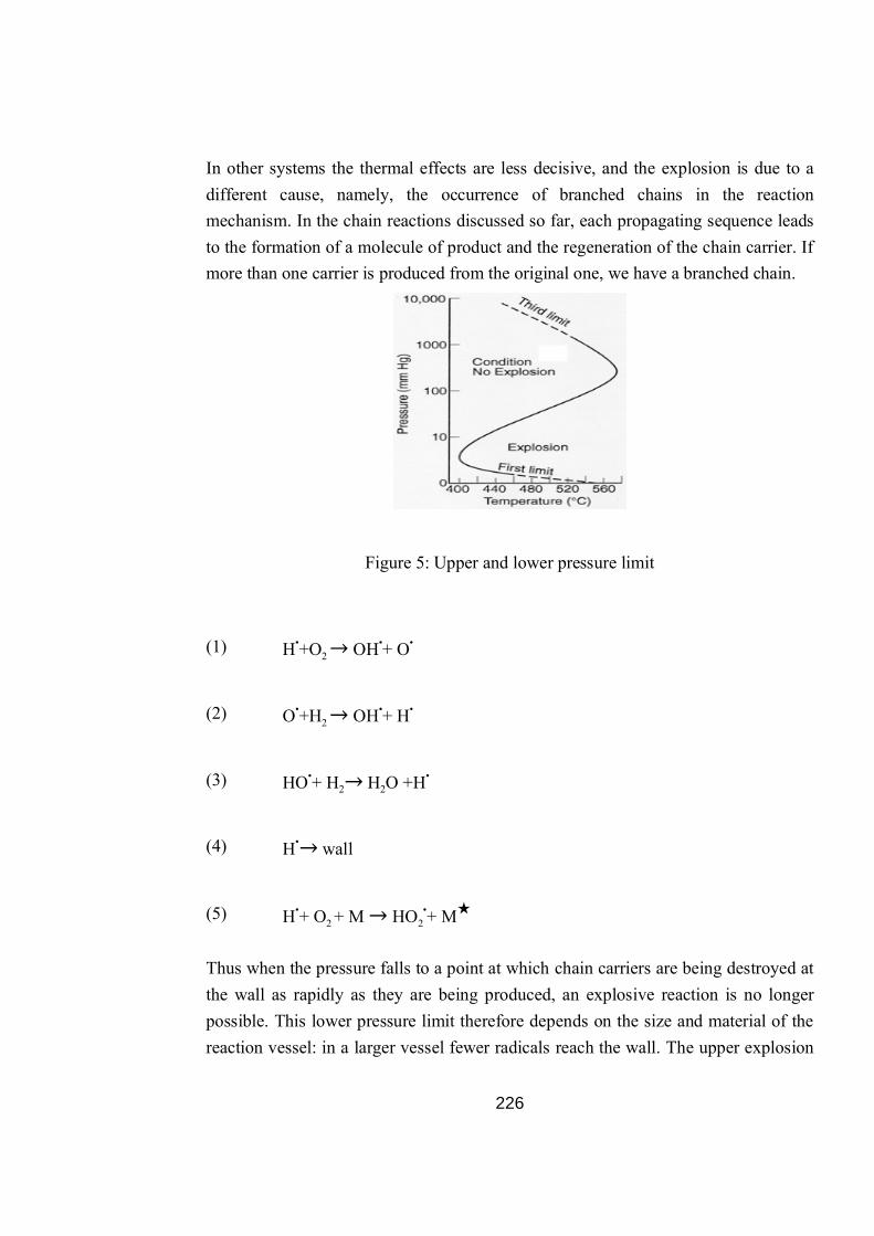
226

In other systems the thermal effects are less decisive, and the explosion is due to a different cause, namely, the occurrence of branched chains in the reaction mechanism. In the chain reactions discussed so far, each propagating sequence leads to the formation of a molecule of product and the regeneration of the chain carrier. If more than one carrier is produced from the original one, we have a branched chain.

Figure 5: Upper and lower pressure limit

Thus when the pressure falls to a point at which chain carriers are being destroyed at the wall as rapidly as they are being produced, an explosive reaction is no longer possible. This lower pressure limit therefore depends on the size and material of the reaction vessel: in a larger vessel fewer radicals reach the wall. The upper explosion

(1) H•+O2 → OH•+ O•

(2) O•+H2 → OH•+ H•

(3) HO•+ H2→ H2O +H•

(4) H•→ wall

(5) H•+ O2 + M → HO2•+ M★

227

limit is reached when destructive collisions in the gas phase outweigh the chain branching. This upper limit usually increases sharply with temperature, because the chain initiating and propagating steps have appreciable activation energy, whereas the chain breaking steps, being re-combinations of atoms or radicals, need little activation energy. In fact, the presence of a third body is often required to carry off the excess energy generated in the highly exothermic recombination reactions. The velocity above the upper pressure limit often becomes so great that the reaction passes over into a thermal explosion.

Actually, the reaction mechanism includes more than 50 elementary reactions. However, in order to understand the main features of the process we will limit ourselves by the five following reactions:

Reactions (1) and (2) are the reactions of branching, since in these reactions one free valence produces three valences. Thus, the number of free valences increases as a result of these reactions. Since the reaction (1) has higher activation energy than reaction (2), the rate of this reaction is slower and it usually can be consider as a rate determining step. Reaction (3) is the reaction of the chain propagation, since it does not change the number of valences. In reactions (4) and (5) the number of valences decreases and these reactions are called chain termination or chain breaking reactions. Note, that the reaction (5) actually looks as a chain propagation reaction, but radical HO2 is rather non-active radical and therefore it will much faster decay on the wall than react with other molecules in the gas phase. Thus, for the simplicity the reaction (5) can be considered as the termination reaction and HO2 as a final product of the total reaction.

This reaction scheme illustrates the ability of branching reactions to create extremely rapid growth in the number of chain carriers and the number of parallel elementary reactions. Whether or not a chain reaction ultimately leads to explosion depends on a number of factors such as the ratio of chain termination to chain branching processes, the initial concentration of reactants (which is a function of pressure for gas reactants such as H2 and O2), the temperature, and the rate at which energy (principally heat) can dissipate from the system. The complex dependence of H2/O2 explosion on pressure and temperature is shown in Figure 9.5. The presence of a complex boundary between steady reaction and explosion reflects competition between the rates of different temperature and pressure dependent reactions in the mechanism. The system is difficult to interpret analytically because the steady state

228

approximation (in which concentrations of reaction intermediates are assumed to remain constant) is not valid under the non-linear conditions of chain branching.

9.12 State true/false

a) Enzyme kinotees is guienly michaelis menten equation. (T/F)

b) Rate of enzymediated reaction is second order with respect to enzyme con

centration (T/F)

c) When culistrate concentration is sufficrenty high, the ouerall rate of reaction is

zero order. (T/F)

d) The upper explosion limit is strongly temperative independent (T/F)

e) The lower pressure limit depends on the size and natural of the reaction vessal

(T/F)

f) During deeompositon of water, it is separated into oxygen and CO2 (T/F).

9.10 Decomposition of water

Decomposition of water is a chemical reaction in which water is separated into oxygen and hydrogen. Efficient and economical water decomposition would be a key technology component of a hydrogen economy. In photosynthesis, this process donates electrons to power the electron transport chain in photosystem II. Water decomposition can be done by using some techniques such as electrolysis, thermal decomposition of water and by chemical methods.

9.10.1 Electrolysis

Electrolysis of water is the decomposition of water intoO2and H2due to an electric current being passed through the water. One important use of electrolysis of water is to produce hydrogen (Figure 9.6). Electrolysis can be done in high pressure and high temperature.

229

Figure 9.6: Electrolysis of Water

(i) High Pressure Electrolysis

In this method, high pressure of about 120–200 bar (1740–2900 psi), at which the produced hydrogen gas is compressed is applied on water. By this process the need for an external hydrogen compressor is eliminated, the average energy consumption for internal compression is around 3%.

(ii) High-Temperature Electrolysis

In this process the supply of energy is in the form of heat (solar thermal, or nuclear). In contrast with low-temperature electrolysis, High-Temperature Electrolysis (THE) of water converts more of the initial heat energy into chemical energy (hydrogen), potentially doubling efficiency to about 50%. Because some of the energy in HTE is supplied in the form of heat, less of the energy must be converted twice (from heat to electricity, and then to chemical form), and so less energy is lost.

Production of hydrogen from water requires large amounts of energy and is uncompetitive with production from coal or natural gas. Potential electrical energy supplies include hydropower, wind turbines, or photovoltaic cells. Usually, the electricity consumed is more valuable than the hydrogen produced so this method has not been widely used. Other potential energy supplies include heat from nuclear reactors and light from the sun.

230

9.10.2 Thermal Decomposition of Water

Thermal decomposition, also called thermolysis, is defined as a chemical reaction whereby a chemical substance breaks up into at least two chemical substances when heated. At elevated temperatures water molecules split into their atomic components hydrogen and oxygen. For example at 2200 °C about three percent of all H2O molecules are dissociated into various combinations of hydrogen and oxygen atoms, mostly H, H2, O, O2, and OH. Other reaction products like H2O2 or HO2 remain minor. At the very high temperature of 3000 °C more than half of the water molecules are decomposed, but at ambient temperatures only one molecule in 100 trillion dissociates by the effect of heat. However, catalysts can accelerate the dissociation of the water molecules at lower temperatures.

9.10.3 Chemical production

A variety of materials react with water or acids to release hydrogen. Such methods are non-sustainable. In the presence of sodium hydroxide, aluminum and its alloys react with water to generate hydrogen gas. Unfortunately, due to its energetic inefficiency, aluminum is expensive and usable only for low volume hydrogen generation. Also high amounts of waste heats must be disposed.

Although other metals can perform the same reaction, aluminum is among the most promising materials for future development, because it is safer, cheaper and easier to transport than some other hydrogen storage materials like sodium borohydride.

Overall reaction of aluminum metal with water is

Al + 3 H2O →Al(OH)3 + 1.5 H2

Since the oxidation of aluminum is exothermic, these reactions can operate under mild temperatures and pressures, providing a stable and compact source of hydrogen. This chemical reduction process is especially suitable for back-up, remote or marine applications. While the passivation of aluminum would normally slow this reaction considerably, its negative effects can be minimized by changing several experimental parameters such as temperature, alkali concentration, physical form of the aluminum, and solution composition.

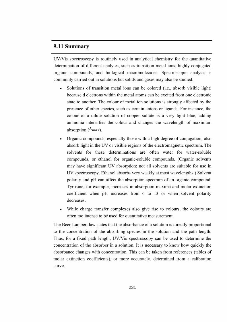
231

9.11 Summary

UV/Vis spectroscopy is routinely used in analytical chemistry for the quantitative determination of different analytes, such as transition metal ions, highly conjugated organic compounds, and biological macromolecules. Spectroscopic analysis is commonly carried out in solutions but solids and gases may also be studied.

Solutions of transition metal ions can be colored (i.e., absorb visible light) because d electrons within the metal atoms can be excited from one electronic state to another. The colour of metal ion solutions is strongly affected by the presence of other species, such as certain anions or ligands. For instance, the colour of a dilute solution of copper sulfate is a very light blue; adding ammonia intensifies the colour and changes the wavelength of maximum absorption ( ).

Organic compounds, especially those with a high degree of conjugation, also absorb light in the UV or visible regions of the electromagnetic spectrum. The solvents for these determinations are often water for water-soluble compounds, or ethanol for organic-soluble compounds. (Organic solvents may have significant UV absorption; not all solvents are suitable for use in UV spectroscopy. Ethanol absorbs very weakly at most wavelengths.) Solvent polarity and pH can affect the absorption spectrum of an organic compound. Tyrosine, for example, increases in absorption maxima and molar extinction coefficient when pH increases from 6 to 13 or when solvent polarity decreases.

While charge transfer complexes also give rise to colours, the colours are often too intense to be used for quantitative measurement.

The Beer-Lambert law states that the absorbance of a solution is directly proportional to the concentration of the absorbing species in the solution and the path length. Thus, for a fixed path length, UV/Vis spectroscopy can be used to determine the concentration of the absorber in a solution. It is necessary to know how quickly the absorbance changes with concentration. This can be taken from references (tables of molar extinction coefficients), or more accurately, determined from a calibration curve.

232

A UV/Vis spectrophotometer may be used as a detector for HPLC. The presence of an analyte gives a response assumed to be proportional to the concentration. For accurate results, the instrument's response to the analyte in the unknown should be compared with the response to a standard; this is very similar to the use of calibration curves. The response (e.g., peak height) for a particular concentration is known as the response factor.

The wavelengths of absorption peaks can be correlated with the types of bonds in a given molecule and are valuable in determining the functional groups within a molecule. The Woodward-Fieser rules, for instance, are a set of empirical

observations used to predict λmax, the wavelength of the most intense UV/Vis absorption, for conjugated organic compounds such as diene and ketones. The spectrum alone is not, however, a specific test for any given sample. The nature of the solvent, the pH of the solution, temperature, high electrolyte concentrations, and the presence of interfering substances can influence the absorption spectrum. Experimental variations such as the slit width (effective bandwidth) of the spectrophotometer will also alter the spectrum. To apply UV/Vis spectroscopy to analysis, these variables must be controlled or accounted for in order to identify the substances present

Although UV-visible spectra do not enable absolute identification of an unknown compound, UV spectra and Visible spectra can be used to identify a compound by comparative analysis. One can compare the UV or Visible spectra of the unknown with the spectra of known suspects.

Besides detecting the presence of distinctive chromophores in a molecule, UV/VIS spectroscopy can also be used to use to detect the extent of conjugation in a molecule, more the conjugation the longer the wavelength of absorption. Each additional double bond in the conjugated pi-electron system shifts the absorption maximum about 30 nm towards longer wavelength. This is due to decreasing energy gap between HOMO and LUMO as the conjugation increases.

UV/vis spectroscopy can also use be used to study geometric isomerism of molecules. The trans isomer absorbs at longer wavelength with a larger molar extinction constant than cis isomer. This can be explained by the steric strain

introduced in the cis isomer resulting in lesser π orbital overlap.

233

UV/Vis spectroscopy can also be used to study the degree of strain; the degree of conjugation may suffer in strained molecules (e.g 2-substitued biphenyls) by correlating changes in spectrum with angular distortion. It can also be used to distinguish the most stable tautomeric forms. The UV spectrum of the solution will be found to be complimentary to more abundant tautomer.

The equilibrium has been shown to lie far to the right, i.e., the UV spectrum of the solution resembles that of the prid-2-one rather than 2-hydroxy pyridine.

9.12 Glossary

Honogcnous catalysis : Catysts is in the same phase as the reatent.

Hetrignous catalysis : Catalyet is in different physical phase from reations.

Autocata lysis: One of the product of reaction itself act as a catalyet for that

reaction.

Thermlysis : Chemical reaction lreaks up into at least two chemical substaneces

when heated.


9.1 a) autocatalyst b) Chemical Compositions c) Content calatysis d) specific

9.2 a) T b) F c) T d) F e) T f) F

9.12 Review Questions:

1. Consider the following mechanism for the enzyme catalyzed reaction:

Derive an expression for the rate law of the reaction in terms of the concentrations of E and S. (Hint: To solve for [ES], make use of the fact that, at equilibrium, the rate of forward reaction is equal to the rate of the reverse reaction.)

234

2. Distinguish between homogeneous catalysis and heterogeneous catalysis. Describe three important industrial processes that utilize heterogeneous catalysis.

3. Illustrate the lowering of Gibbs free energy of activation of a reaction by a catalyst. Discuss carefully the general characteristics of catalytic reactions.

4. Discuss the mechanism and kinetics of enzyme catalyzed reactions. 5. What are enzyme catalysts? Explain with examples. 6. Discuss briefly about explosive reactions with suitable examples. 7. Explain various methods for decomposition of water. 8. Discuss the kinetics of following photochemical reaction.

9. Derive the expression:


1. B.R. Puri, L.R. Sharma, M.S. Pathania, Principles of Physical Chemistry, Vishal Publishing Coporation, Jalandhar, 2012.

2. Physical Chemistry – G. M. Barrow, Tata-McGraw Hill, Vth edition, 2003. 3. A.G. Whittaker, A.R. Mount, M.R. Heal, Physical Chemistry, BIOS Scientific

Publishers Limited, 2000. 4. Arun Bahl, G.S. Bahl, G.D. Tuli, Essentials of Physical Chemistry, Ed. S. Chand,

2011.

H2(g) + Br2(g) 2HBr(g)h

d[HBr]

dt= k[H2][Br2]3/2

235

Unit - 10 Fast Reactions Structure of Unit

10.0 Objectives

10.1 Introduction

10.2 Characteristics of fact reactions

10.3 Difference between slow and fast reactions

10.4 Flow techniques

10.5 Flash photolysis method

10.6 Chemical relaxation method

10.7 NMR techniques

10.8 Summary

10.9 Glossary


10.10 Review question

10.11 Reference and suggested readings

10.0 Objectives At the end of the chapter the student will able to :-

To understand differ between slow reaction and fast reaction.

To know characteritics of fast reactions.

To study flow techniques continuous or stopped flow technique.

To understand flash photohysis technique.

To understand principle of chemical relaxation method.

To define relaxation time and its derivation

To understand underlying principle for NMR technique.

10.1 Introduction As we all know that chemical kinetics is a branch of science which deals with speed of reaction or the rate at which con centration of reaetant charges with time. Their are various types of reactions as simple chemical reactions chain reactios, polymerisation

236

reactions and fast reactions. A chain reaction is one in which the products of the reaction carry on reaction on the part of reacting molecules. As a result a long series of self repeating steps are started. Polymerisation reaction are the reactions in which a number of molecules react to form a large molecule. Similarly their are some reactions which go to the equilibriuim in a few seconds or less. Those reactions are called as fast reactions. These are very rapid reactions and conventional techniques are not able to study these reactions. In this chapter we will study various techniques to study fast reactions.

10.2 Characteristics of Fast Reactions These are those chemical reactions which go to the equilibirium is a few seconds or

even less than that. They complete in even 10-13 see. Conventional techniques can not be used to study these reactions as error will be made because the initial time can not be determind accurately. Also the time it takes to make a measurement of centration may be significant compared to halylife. As a result special analytical methods and experimental techniques are used for study these fast reactions.

a) These reaction are so fast that they occur as soon as the reatants are

brought together. These reactions take about 10-14 to 10-16 see for completion. It is almost impossible to determine the rates of these reactions eg.

AgNO3 + NaCl AgCl + NaNO3

NaOH + HCl NaCl + H2O

b) They have a half life of milli second or less

c) Special experimental techniques are used to study these reactions.

d) They take place instantaneously

e) The time it takes to mix reactants or to bring them to a desired temperature may be significant as compared to the half life to the reaction.

f) Kinetic data in solutions are obtained by NMR techniques. The method is based on the fact that when two compounds with different NMR chemical shift change rapidly from one to another, their two peaks merge into one.

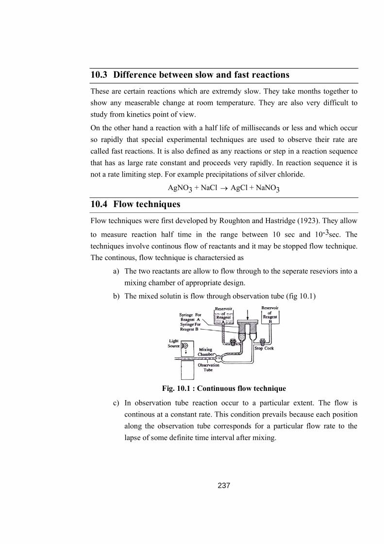
237

10.3 Difference between slow and fast reactions These are certain reactions which are extremdy slow. They take months together to show any measerable change at room temperature. They are also very difficult to study from kinetics point of view.

On the other hand a reaction with a half life of millisecands or less and which occur so rapidly that special experimental techniques are used to observe their rate are called fast reactions. It is also defined as any reactions or step in a reaction sequence that has as large rate constant and proceeds very rapidly. In reaction sequence it is not a rate limiting step. For example precipitations of silver chloride.

AgNO3 + NaCl AgCl + NaNO3

10.4 Flow techniques Flow techniques were first developed by Roughton and Hastridge (1923). They allow

to measure reaction half time in the range between 10 sec and 10-3sec. The techniques involve continous flow of reactants and it may be stopped flow technique. The continous, flow technique is charactersied as

a) The two reactants are allow to flow through to the seperate reseviors into a mixing chamber of appropriate design.

b) The mixed solutin is flow through observation tube (fig 10.1)

Fig. 10.1 : Continuous flow technique

c) In observation tube reaction occur to a particular extent. The flow is continous at a constant rate. This condition prevails because each position along the observation tube corresponds for a particular flow rate to the lapse of some definite time interval after mixing.

238

d) Since with a constant flow rate, the concentrations at a particular point along observation tube do not change so it is possible to make observation in a few milliseconds after mixing.

e) Light is allow to fall on the observation tube through light source.

f) The extent of reaction is determined if the absorption spectrum of the product differs from that of the reactant.

g) The spectro photometrie equipment ie set up at a point down stream from the point on mixing

h) Value of light abservation at particular point provide a data from which a plot of extent of reaction versus time can be prepared.

i) From observations extent of reaction can be determined.

10.4.1 Stopped flow technique The flow techniques are the logical extension of the classical mix and shake method in which the reactants are now mixed with in a praction of a second.

In stopped flow technique the flow is stopped suddenly and them the rate at which the system reaches equilibrium can be followed by measuring. The concentration change of a reactant or a product as a fuction of time. The following reactants get discharged after rapid mixing. They get it into a quenching solution to arrest the reaction. Since the flow is stopped suddenly so their is rapid change in the concentration of reactants and is observed spectro photo metrically. The change in the concentration of reactant before and after mixing will give kinetics of reactions.

10.5 Flash photolysis method The method was frist given by Porter (1950). It is now widely used in investigating reactions in solution. The principle behind is to apply a large peturbation (disturbance) to a system and generating one of the reactants and then follow the disappearence of this reactivre specees. This is characterised as follows -

a) The reactants are placed in a cylindrical quartz veisel 50 cm long and 2cm india meter.

b) It is mounted to photolysis flash tube.

c) Next to it is a quartz tube which is filled with rare gas, Krypton.

d) The reaction vessel and flash lamp is mounted in a hollow cylinder and whole inner surface is coated with magnesuim oxide.

239

e) Conden cers are connected to a electrode and they get charge by applying required voltage (fig 10.2)

Fig. 10.2 : Typical flash-photolysis apparatus

j) The condensers get discharged by applying a triggering pulse to a small central electrode.

g) The duration time of the photolysis flash depends on the energy to be dissipated.

h) The lasers can produce a flash of the durations of a new nano second. After then the flash lamp is automatically triggered off. The rate of disappearance of excited molecule or free radicals is followed by the rate of increase in monochromatie transmnitted light as measured with photomultiplier.

i) When a flash is applied the system get perturbed vary rapidly from equilibrium and change in concentrations will take place. This will noted down by spectrophotometer and will help in determining kinetics of fast reactions.

10.6 Chemical relaxation method In relaxation techniques a system is perturbed or chemical equilibrium is disturbed by a rapid change in one of the several possible external parameters. For example change in electricfield intensity, temperature or pressure. The ralaxation is them followed by spectro photometer or conductometer techniques. The time during which reaction get relaxed from equilibrium is called as relaxation time. This can be determined mathematically.

The relaxation time can be determined by various methods like temperature jump and pressure jum methods. Let us consider one by one.

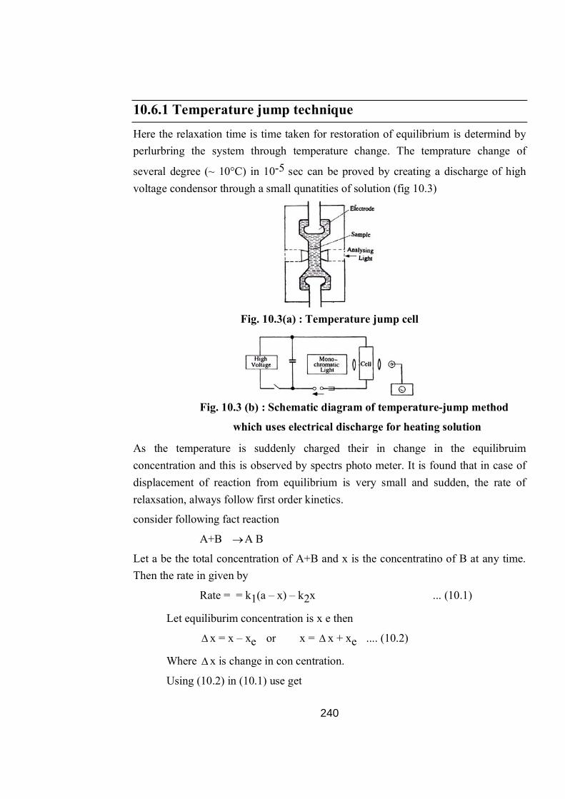
240

10.6.1 Temperature jump technique Here the relaxation time is time taken for restoration of equilibrium is determind by perlurbring the system through temperature change. The temprature change of

several degree (~ 10°C) in 10-5 sec can be proved by creating a discharge of high voltage condensor through a small qunatities of solution (fig 10.3)

Fig. 10.3(a) : Temperature jump cell

Fig. 10.3 (b) : Schematic diagram of temperature-jump method

which uses electrical discharge for heating solution

As the temperature is suddenly charged their in change in the equilibruim concentration and this is observed by spectrs photo meter. It is found that in case of displacement of reaction from equilibrium is very small and sudden, the rate of relaxsation, always follow first order kinetics.

consider following fact reaction

A+B A B

Let a be the total concentration of A+B and x is the concentratino of B at any time. Then the rate in given by

Rate = = k1(a – x) – k2x ... (10.1)

Let equiliburim concentration is x e then

x = x – xe or x = x + xe .... (10.2)

Where x is change in con centration.

Using (10.2) in (10.1) use get

241

= k1(a – xe – x) – k2(xe – x) .... (10.3)

At equilibruim = 0 and x = ee so

k1(a – xe) = k2 xe . .. (10.4)

Substituting the value we get

Rate = – (k1 + k2) x

or = – kT x ... (10.5)

Where KT = (k1 + k2) and is called as relaxation rate conetant

The reciprocal of kT that is (k1 + k2)–1 is called as relaxation time. it is deneted by

t (Tou). So

t = 1 2

1k k = T

1k .... (10.6)

When t is relaxation time. This plays very important role in chemical kinetics and help to determine the time by which system is restored for equilibrium. 10.6.2 Pressure Jump technique

Here the sudden charge of pressure is applied to displace the system from equilibrium. The sensitivity of reaction depends on the change in volume and represented as

T

ln kp

=

0– VRT

... (10.7)

Where V0 is change is volume by application of pressure.

The sample is placed in a flexible cell. It is then connected in a pressure vessel filled with an inert liquid. Then a pressure of about 65 atmpsospheres is set up in the

vessel. The pressure is then redused to a atmospheric pressure in about 10-4 sec by puncting a thin metal driecet into the wall of vessel (fig 10.4)

Fig 10.4 : Pressure jump techneque

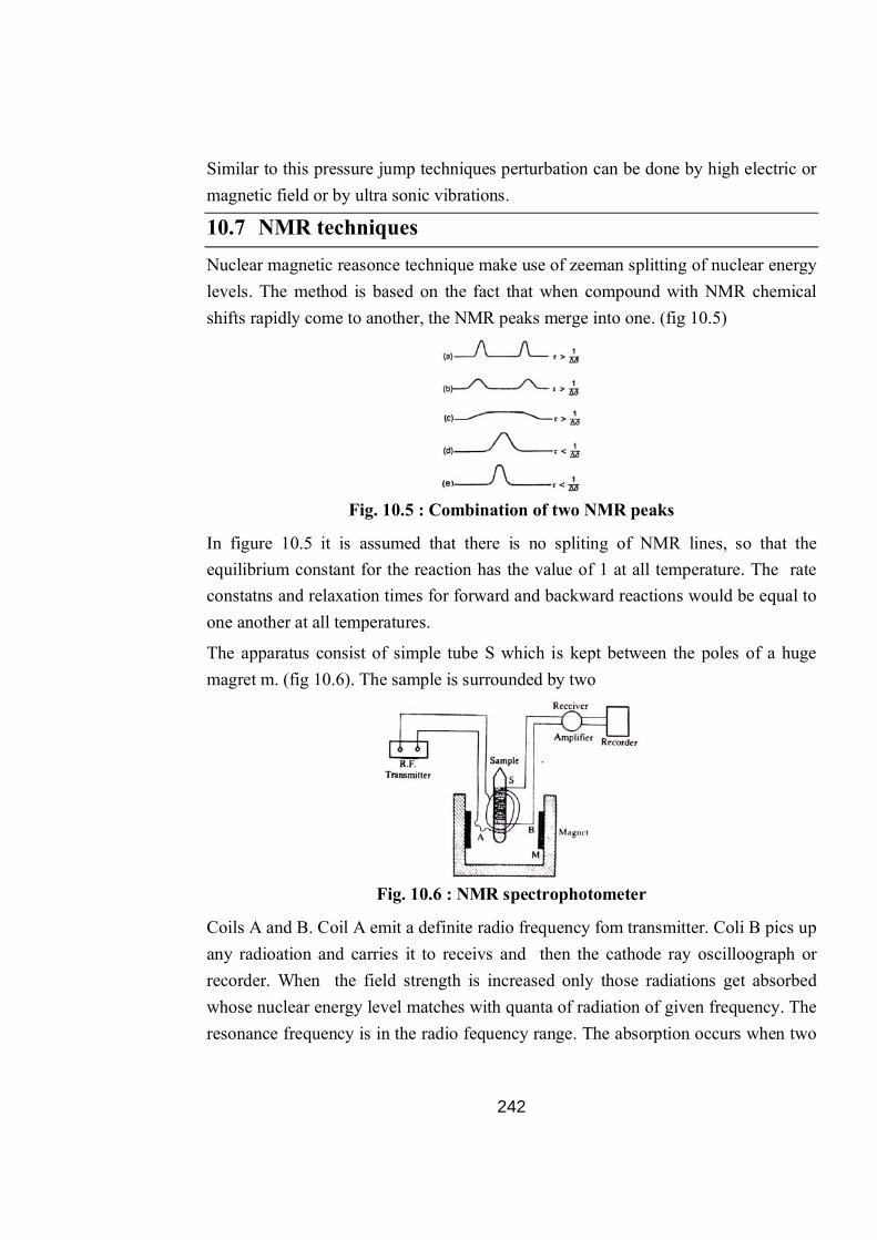
242

Similar to this pressure jump techniques perturbation can be done by high electric or magnetic field or by ultra sonic vibrations.

10.7 NMR techniques Nuclear magnetic reasonce technique make use of zeeman splitting of nuclear energy levels. The method is based on the fact that when compound with NMR chemical shifts rapidly come to another, the NMR peaks merge into one. (fig 10.5)

Fig. 10.5 : Combination of two NMR peaks

In figure 10.5 it is assumed that there is no spliting of NMR lines, so that the equilibrium constant for the reaction has the value of 1 at all temperature. The rate constatns and relaxation times for forward and backward reactions would be equal to one another at all temperatures.

The apparatus consist of simple tube S which is kept between the poles of a huge magret m. (fig 10.6). The sample is surrounded by two

Fig. 10.6 : NMR spectrophotometer

Coils A and B. Coil A emit a definite radio frequency fom transmitter. Coli B pics up any radioation and carries it to receivs and then the cathode ray oscilloograph or recorder. When the field strength is increased only those radiations get absorbed whose nuclear energy level matches with quanta of radiation of given frequency. The resonance frequency is in the radio fequency range. The absorption occurs when two

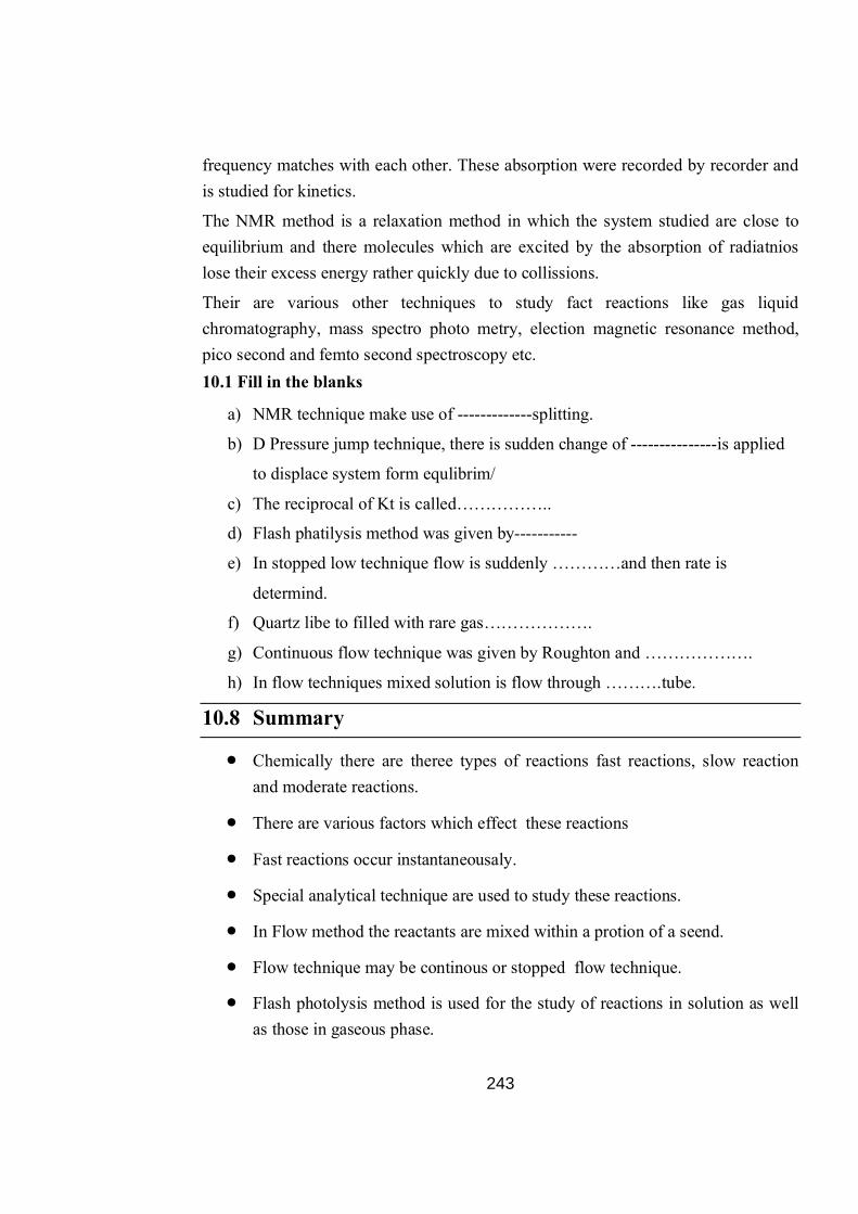
243

frequency matches with each other. These absorption were recorded by recorder and is studied for kinetics.

The NMR method is a relaxation method in which the system studied are close to equilibrium and there molecules which are excited by the absorption of radiatnios lose their excess energy rather quickly due to collissions.

Their are various other techniques to study fact reactions like gas liquid chromatography, mass spectro photo metry, election magnetic resonance method, pico second and femto second spectroscopy etc. 10.1 Fill in the blanks

a) NMR technique make use of -------------splitting.

b) D Pressure jump technique, there is sudden change of ---------------is applied

to displace system form equlibrim/

c) The reciprocal of Kt is called……………..

d) Flash phatilysis method was given by-----------

e) In stopped low technique flow is suddenly …………and then rate is

determind.

f) Quartz libe to filled with rare gas……………….

g) Continuous flow technique was given by Roughton and ……………….

h) In flow techniques mixed solution is flow through ……….tube.

10.8 Summary

Chemically there are theree types of reactions fast reactions, slow reaction and moderate reactions.

There are various factors which effect these reactions

Fast reactions occur instantaneousaly.

Special analytical technique are used to study these reactions.

In Flow method the reactants are mixed within a protion of a seend.

Flow technique may be continous or stopped flow technique.

Flash photolysis method is used for the study of reactions in solution as well as those in gaseous phase.

244

In relaxation method a chemical equilibrium is perturbed by a rapid change in one of the several parameters like pressure, temperature, electricfield intensity etc. The process is then followed by spectro photometric analysis.

Relaxation technique can be temperature jump or pressure jump method.

The NMR method is a relaxation method in which the systems studied are usually close to equilibrium and those molecules which are excited by the absorption of radiation lose their excess energy rather quickly due to callissuon.


10.1 a) Zeeman b) Presure c) relaxatation d) Porter e) stopped

f)krypton g) Hostridge

10.9 Review Questions A) Short Answer Type

1. What do you mean by fast reactions?

2. Differntiate between Slow and fast reactions?

3. State the principle behind flow techniques?

4. Define relaxation time?

5. What do you understand by temperature jump technique? B) Long Answer Type

1. Give characteristics of fast reactions. Differentiate between continous flow and stopped flow technique.

2. Describe flash photolysis method to study fast reaction.

3. Discuss chemical relaxation technique with reference to temperature jump method

4. What do you understand by relaxation time? Define it relation with rate constants. How it is different from pressure jump method.

5. How NMR technique is used to study fast reactions? Give instrumentation analysis also.

245

6. Explain any two techniques to study fast reactions. Also charaterize fast reactions?

10.10 References and suggested readings 1. Advanced physical chemistry - Gurdeep Raj

2. Physical chemistry - R.S. Rastogi

3. Physical chemistry - David W. Ball

4. Physical chemistry - G.K. Vemulapalli

5. Physical chemistry - Puri, Sharma and Patania

6. Chemical Kinetics - Keith J Laidler

246

Unit-11 : Collision Theory Structure of unit

11.1 Objective

11.2 Introduction

11.3 Basic concept of collision theory

11.4 Demerits of collision theory

11.5 Steric Factor

11.6 Transition State Theory or Activated Complex Theory

11.7 Eyring Equation


11.9 Summary

11.10 Glossary




11.1 Objectives

There are many concepts which explains how chemical reaction occurs but collision theory was the first theory by which progress of a chemical reaction was explained. That’s why collision theory is supposed to study first than any other theory or concept.

11.2 Introduction

This chapter basically deals with the collision theory. One can understand following topics by study the chapter:

247

Basic concept of collision theory and its demerits


Transition state theory, its limitations and applications

Eyring equation and its difference from Arrhenius equation

11.3 Basic concept of collision theory

Generally, rate of a reaction is expressed in terms of a rate constant multiplied by a function of concentrations of reactants. As a result, it is the rate constant that contains information related to the collision frequency, which determines the rate of a reaction in the gas phase. When the rate constant is given by the Arrhenius equation,

…………(11.1)

Ea is related to the energy barrier over which the reactants must pass as products form. For molecules that undergo collision, the exponential is related to the number of molecular collisions that have the required energy to induce reaction. The pre-exponential factor, A, is related to the frequency of collisions. Therefore, we can describe the reaction rate as

Rate = (Collision frequency) x (Fraction of collisions with at least the threshold energy)

or

…………(11.2)

where Z is the frequency of coffisions between molecules of A and B and F is the fraction of those collisions having sufficient energy to cause reaction.

The collision frequency between two different types of molecules can be calculated by means of the kinetic theory of gases. In this discussion we will consider the molecules of B as being stationary and A molecules moving through a collection of them. If we imagine a molecule of A moving through space where molecules of B are located, collisions will occur with molecules of B whose centers lie within a cylinder of length vAB and radius rA + rB where V1sj is the average relative velocity of A and B and rA + rB is the sum of the radii of molecules A and B. A diagram showing this situation is shown in the following figure

248

Fig 11.1 Colbrision between mabuba A and B

If the cross sectional area of the cylinder, π(rA + rB)2, the collisional cross section, is

σAB In 1 second, a molecule of A travels a distance of vAB (where vAB is the average molecular velocity of A relative to B) and it will collide with all molecules of B that have centers that lie within the cyllnder. Therefore, the number of collisions per second will be given by the number of B molecules/cm3 multiplied by the volume of the cylinder. This can be expressed by the equation

Although A does not continue in a straight line after colliding with B, the calculated collision frequency will still be correct as long as there is no gradient in concentration of B within the container and the velocity of A remains constant. The preceding result is for a single molecule of A. To obtain the total number of collisions between molecules of A and B, Z, the result must be multiplied by CA, the number of molecules of A per cm3. Therefore, the collision frequency is

…………(11.4)

Because we have considered molecules of B to be stationary (velocity = 0), the relative velocity is just the root-mean-square velocity of A,

…………(11.5)

where T is the temperature (K), k is Boltzmann’s constant, and m is the mass of A. Note that Boltzmann’s constant is denoted in bold to distinguish it from a rate

constant. If we represent the reduced mass of a pair of molecules A and B as μ, then

or, in the more familiar form,

249

…………(11.6)

The relative velocity of A and B can now be written as

Having derived an expression for the relative velocity of the molecules, the collision frequency is expressed as

…………(11.7)

Frequently, the collision diameter, d = (dA + dB)/2, is used and the concentrations are written in terms of numbers of molecules/cm3, nA and nB, per unit volume. Then,

……………(11.8)

One factor that has been ignored to this point is that although a collision frequency can be calculated, the collision between the molecules must occur with sufficient energy for the reaction to occur. As we have previously seen, that minimum energy is the activation energy. Following figure shows a Maxwell-Boltzmann distribution of energies of gaseous molecules.

11.4 Demerits of collision theory

The demerits of collision theory are as follows,

1. Collision theory does not provide any prediction of p, the “steric factor”.

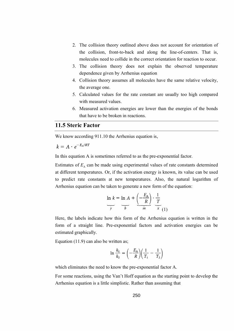
250

2. The collision theory outlined above does not account for orientation of the collision, front-to-back and along the line-of-centers. That is, molecules need to collide in the correct orientation for reaction to occur.

3. The collision theory does not explain the observed temperature dependence given by Arrhenius equation

4. Collision theory assumes all molecules have the same relative velocity, the average one.

5. Calculated values for the rate constant are usually too high compared with measured values.

6. Measured activation energies are lower than the energies of the bonds that have to be broken in reactions.

11.5 Steric Factor

We know according 911.10 the Arrhenius equation is,

In this equation A is sometimes referred to as the pre-exponential factor.

Estimates of EA can be made using experimental values of rate constants determined at different temperatures. Or, if the activation energy is known, its value can be used to predict rate constants at new temperatures. Also, the natural logarithm of Arrhenius equation can be taken to generate a new form of the equation:

(1)

Here, the labels indicate how this form of the Arrhenius equation is written in the form of a straight line. Pre-exponential factors and activation energies can be estimated graphically.

Equation (11.9) can also be written as;

which eliminates the need to know the pre-exponential factor A.

For some reactions, using the Van’t Hoff equation as the starting point to develop the Arrhenius equation is a little simplistic. Rather than assuming that

251

……..(11.10)

By including the temperature term, above equation becomes

or

……..(11.11)

For m = 0, above equation reduces into the Arrhenius equation some as (11.1).

The pre-exponential factor, which is a constant for a given reaction must have a value that is dictated by the specifics of the reaction itself, like the nature of the reactants and how they interact on a molecular level.

One of the most obvious is the number of molecules that are colliding. The number of collisions is calculable from kinetic theory. For example, at the end of that section we showed that the total number of collisions per second per unit volume, represented by Z, is given by

……..(11.12)

whered1 and d2 are the diameters of gas particles in species 1 and 2, and μ is the reduced mass of two particles of those species. If the effect of temperature changes is minor compared to the exponential term in the Arrhenius equation (that is, the -EA/RTe

term), and if the densities of the two species ρ1 and ρ2 are converted to concentrations and separated from the rest of the expression, then it can be assumed that the rest of the expression is approximately constant, i. e.

…………..(11.13)

This one factor, a collision frequency factor, is one major contribution to the pre-exponential constant A.

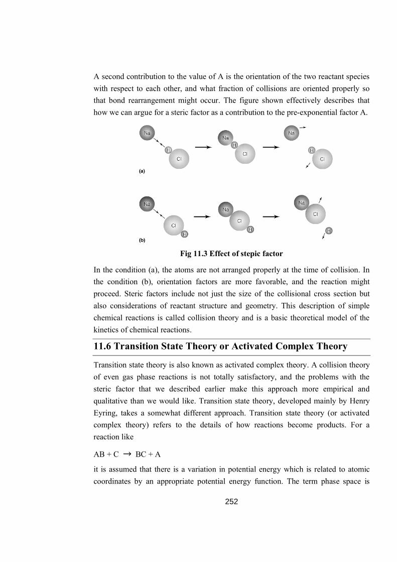
252

A second contribution to the value of A is the orientation of the two reactant species with respect to each other, and what fraction of collisions are oriented properly so that bond rearrangement might occur. The figure shown effectively describes that how we can argue for a steric factor as a contribution to the pre-exponential factor A.

Fig 11.3 Effect of stepic factor

In the condition (a), the atoms are not arranged properly at the time of collision. In the condition (b), orientation factors are more favorable, and the reaction might proceed. Steric factors include not just the size of the collisional cross section but also considerations of reactant structure and geometry. This description of simple chemical reactions is called collision theory and is a basic theoretical model of the kinetics of chemical reactions.

11.6 Transition State Theory or Activated Complex Theory

Transition state theory is also known as activated complex theory. A collision theory of even gas phase reactions is not totally satisfactory, and the problems with the steric factor that we described earlier make this approach more empirical and qualitative than we would like. Transition state theory, developed mainly by Henry Eyring, takes a somewhat different approach. Transition state theory (or activated complex theory) refers to the details of how reactions become products. For a reaction like

AB + C → BC + A

it is assumed that there is a variation in potential energy which is related to atomic coordinates by an appropriate potential energy function. The term phase space is

253

applied to the coordinate and momentum space for the system. For a reaction to occur, the transition state must pass through some critical configuration in this space. Because of the nature of the potential function used to express the energy of the system as a function of atomic positions, the system energy possesses a saddle point. This saddle point lies lower in energy than the fully dissociated arrangement, A + B + C, or the highly “compressed” arrangement, A-B-C.

The main feature of transition state theory is that there is a “concentration” of the species at the saddle point, the transition state or activated complex, that is in equilibrium with reactants and products. The Boltzmann Distribution Law governs the concentration of that transition state, and the rate of reaction is proportional to its concentration. The concentration of the transition state is small because of its energy being higher than that of the reactants, hence this critical configuration represents the “regulator” of the rate of flow of reactants to products.

The concentration of the transition state is one of the factor which is involved, since the frequency of its dissociation into products comes into play because the rate at which it decomposes must also be considered. Therefore, the rate can be expressed as

Rate = (Concentration of Transition state) x (Decomposition frequency)

To form a product by the transition state, one bond must acquire sufficient vibrational energy to separate. When it does separate, one of the 3N — 6 vibrational degrees of freedom (for a linear molecule it is 3N — 5) is lost and is transformed into translational degrees of freedom of the products. The main idea of transition state theory is the assumption that the transition state species is in equilibrium with the reactants. Thus,

………(11.14)

For the formation of the transition state, the equilibrium constant is

……………(11.15)

from which we find that the concentration of the transition state is

Since the reaction rate is expressed as the product of the concentration of the transition state and the frequency of its decomposition, we can now write

254

………..(11.16)

As we know that

And since

Therefore, the equilibrium constant for formation of the transition state can be written as

…………(11.17)

By putting this value in the equation (11.16), we get

…………(11.18)

Now we have obtained an expression for the rate in terms of concentrations and thermodynamic quantities, the frequency of decomposition of transition state must now be addressed.

By considering the vibration of the transition state when it is at the top of the potential energy barrier, temperature limit in energy for a vibrational mode can be expressed as

wherek is Boltzmann’s constant and T is the temperature (K). Since k = R/No (where No is Avogadro’s number), hence

Now since,

or

…………...…11.19

255

Because the reaction rate can be expressed in terms of the concentration of the transition state, the rate can now be given by

Substituting for the rate constant gives

Now putting the value of equation (11.19) in the above equation

…………(11.20)

The rate constant can now be written as

…………(11.21)

A somewhat more elegant approach to deriving an expression for the rate of passage over the potential energy barrier is based on statistical mechanics. According to this method, it is assumed that there is a some distance, d, at the top of the barrier, which must be the distance where the transition state exists. It is the distance in which vibrational mode of the complex is transformed into translational motion of the products. The rate of passage of the transition state through distance d is related to the molecular velocity in one direction. If the mass of the transition state is m‡, the average velocity is

or

…………(11.22)

The number of complexes crossing the potential barrier through distance d per unit time is

256

…………(11.23)

Note that we are using []‡ to represent the transition state and [‡] to represent the concentration of the transition state. Now, the concentration of the transition state, [‡], is to be evaluated. If the difference between energies of the zero—point of the reactants and the transition state is Eo

‡, the equilibrium constant for formation of the transition state is given by

…………(11.24)

where QA,OB, and Q‡ are the partition functions of reactants A and B and the transition state, respectively. If the vibrational mode of the transition state is factored out of Q we can write

…………(11.25)

where q‡v is the vibrational mode of the bond being broken. Now we can approximate

the vibrational mode as

and the equilibrium constant K‡ is given by

which is of the same form found earher with the rate constant, k, being given by

…………(11.26)

The resemblance of this equation to the Arrhenius equation is apparent when the pre-exponential factor includes the frequency factor and the equihlirium constant in terms of partition functions. This expression for k is similar to that obtained from collision theory.

257

An approximate rate constant, ka, can be calculated from probability that the reactants in the distribution of quantum state will collide and react in accord with the collision frequency. The approximate constant is greater than the measured rate constant, k. One approach to improving transition state theory with respect to calculating the rate constant is to alter the configuration of the transition state used in the energy calculations in order to effect a change in a. In fact, the calculations are performed in such a way that the calculated rate constant is a minimum and thereby approaches the observed k. Just as energy minimization is accomplished by means of the variation method in quantum mechanical calculations, this procedure is referred to in this connection as variational transition state theory.

Because the free energy of activation is given by

…………….(1.27)

this procedure amounts to configuration optimization to minimize K‡ or maximize

G‡. In practice, a series of transition states is considered and the calculations are performed to obtain the desired minimization. It is of some consequence to choose the reaction path with respect to the energy surface.

Limitations of Transition state theory:

In general, Transition state theory has provided researchers with a conceptual foundation for understanding how chemical reactions take place. Even though the theory is widely applicable, it does have limitations. For example, when applied to each elementary step of a multi-step reaction, the theory assumes that each intermediate is long-lived enough to reach a Boltzmann distribution of energies before continuing to the next step. When the intermediates are very short-lived, however, then TST fails. In such cases, the momentum of the reaction trajectory from the reactants to the intermediate can carry forward to affect product.

It is based on the assumption that atomic nuclei behave according to classic mechanics. It is assumed that unless atoms or molecules collide with enough energy to form the transition structure, then the reaction does not occur. However, according to quantum mechanics, for any barrier with a finite amount of energy, there is a possibility that particles can still tunnel across the barrier. With respect to chemical reactions this means that there is a chance that molecules will react even if they do not collide with enough energy to traverse the energy barrier. While this effect is

258

expected to be negligible for reactions with large activation energies, it becomes a more important phenomenon for reactions with relatively low energy barriers, since the tunneling probability increases with decreasing barrier height.

Transition state theory fails for some reactions which occur high temperature. The theory assumes the reaction system will pass over the lowest energy saddle point on the potential energy surface. While this description is consistent for reactions occurring at relatively low temperatures, at high temperatures, molecules populate higher energy vibrational modes; their motion becomes more complex and collisions may lead to transition states far away from the lowest energy saddle point. This deviation from transition state theory is observed even in the simple exchange reaction between diatomic hydrogen and a hydrogen radical.

Application of transition state theory:

(a) Enzymes catalyze chemical reactions at rates that are astounding relative to uncatalyzed chemistry at the same reaction conditions. Each catalytic event requires a minimum of three or often more steps, all of which occur within the few milliseconds that characterize typical enzymatic reactions. According to transition state theory, the smallest fraction of the catalytic cycle is spent in the most important step, that of the transition state. The original proposals of absolute reaction rate theory for chemical reactions defined the transition state as a distinct species in the reaction coordinate that determined the absolute reaction rate.

Soon thereafter, Linus Pauling proposed that the powerful catalytic action of enzymes could be explained by specific tight binding to the transition state species. Because reaction rate is proportional to the fraction of the reactant in the transition state complex, the enzyme was proposed to increase the concentration of the reactive species.

(b) This proposal was formalized by Wolfenden and coworkers at University of North Carolina at Chapel Hill, who hypothesized that the rate increase imposed by enzymes is proportional to the affinity of the enzyme for the transition state structure relative to the Michaelis complex. Because enzymes typically increase the non-catalyzed reaction rate by factors of 1010-1015, and Michaelis complexes often have dissociation constants in the range of 10−3-10−6 M, it is proposed that transition state complexes are bound with

259

dissociation constants in the range of 10-14 -10−23 M. As substrate progresses from the Michaelis complex to product, chemistry occurs by enzyme-induced changes in electron distribution in the substrate.

(c) Enzymes alter the electronic structure by protonation, proton abstraction, electron transfer, geometric distortion, hydrophobic partitioning, and interaction with Lewis acids and bases. These are accomplished by sequential protein and substrate conformational changes. When a combination of individually weak forces are brought to bear on the substrate, the summation of the individual energies results in large forces capable of relocating bonding electrons to cause bond-breaking and bond-making. Analogs that resemble the transition state structures should therefore provide the most powerful noncovalent inhibitors known, even if only a small fraction of the transition state energy is captured.

(d) All chemical transformations pass through an unstable structure called the transition state, which is poised between the chemical structures of the substrates and products. The transition states for chemical reactions are proposed to have lifetimes near 10-13 seconds, on the order of the time of a single bond vibration. No physical or spectroscopic method is available to directly observe the structure of the transition state for enzymatic reactions, yet transition state structure is central to understanding enzyme catalysis since enzymes work by lowering the activation energy of a chemical transformation.

(e) It is now accepted that enzymes function to stabilize transition states lying between reactants and products, and that they would therefore be expected to bind strongly any inhibitor which closely resembles such a transition state. Substrates and products often participate in several enzyme reactions, whereas the transition state tends to be characteristic of one particular enzyme, so that such an inhibitor tends to be specific for that particular enzyme. The identification of numerous transition state inhibitors supports the transition state stabilization hypothesis for enzymatic catalysis.

(f) Currently there is a large number of enzymes known to interact with transition state analogs, most of which have been designed with the intention of

260

inhibiting the target enzyme. Examples include HIV-1 protease, racemases,

β-lactamases, metalloproteinases, cyclooxygenases and many others.

11.7 Eyring Equation

The Eyring equation ( also known as Eyring–Polanyi equation) is an equation used in chemical kinetics to describe the variance of the rate of a chemical reaction with temperature. It was developed almost simultaneously in 1935 by Henry Eyring, M.G. Evans and Michael Polanyi. This equation follows from the transition state theory (or activated-complex theory) and is trivially equivalent to the empirical Arrhenius equation which are both readily derived from statistical thermodynamics in the kinetic theory of gases.

The general form of the Eyring–Polanyi equation somewhat resembles the Arrhenius equation:

…………(11.28)

whereΔG‡ is the Gibbs energy of activation, k is Boltzmann's constant, and h is Planck's constant.

It can be rewritten as:

k = kTh

S HR RT expexp

…………(11.29)

Where,

k = reaction rate constant

T = absolute temperature

H‡ = enthalpy of activation

R = gas constant

k = Boltzmann constant

k = Planck's constant

S‡ = entropy of activation

261


Transition state theory requires a value of the transmission coefficient k as a prefactor in the Eyring equation above. This value is usually taken to be unity (i.e., the transition state AB‡ always proceeds to products AB and never reverts to reactants A and B). As discussed by Winzor and Jackson in 2006, this assumption invalidates the description of an equilibrium between the transition state and the reactants and therefore the empirical Arrhenius equation is preferred with a phenomenological interpretation of the prefactor A and activation energy Ea.

At first sight this looks like an exponential multiplied by a factor that is linear in temperature. However, one must remember that free energy is itself a temperature dependent quantity. The free energy of activation is the difference of an enthalpy term and an entropy term multiplied by the absolute temperature. When all of the details are worked out one ends up with an expression that again takes the form of an Arrhenius exponential multiplied by a slowly varying function of T. The precise form of the temperature dependence depends upon the reaction, and can be calculated using formulas from statistical mechanics involving the partition functions of the reactants and of the activated complex.

11. 1 State true and false (After 11.8)

a) The collision frequency between two different types of molecules can be

calculated by means of kinatee theory of gases. (T/F)

b) Collision theroty consider stere fartor (T/F)

c) Transition state theory is given by honry eyring (T/F)

Transition state is a stable state (T/F) 11.2 Complete the following

a) Arrhenius equation is ………………….

b) According to collision theory

Zab

c) According to transition state theory

262

11.9 Summary

In this chapter basically the collision theory and transition state theory have been discussed. One can understand following topics by study the chapter:

Basic concept of collision theory and its demerits


Transition state theory, its limitations and applications

Eyring equation and its difference from Arrhenius equation

11.10 Glossary


Reaction rate: The reaction rate (rate of reaction) or speed of reaction for a reactant or product in a particular reaction is defined as how fast or slow a reaction takes place.





Answer tokey assessement question

11.1 a) T b) F c) T d)F

11.2 a) K=Ae—EaIRT b) ABCACB c) KT /h d)

263


1. Write short note on collision theory. 2. What are the demerits of collision theory? 3. What do you understand by steric factor for a chemical reaction? 4. How steric factor play an important role for a chemical reaction? Discuss with

diagram. 5. Discuss collision theory in detail. 6. Write short note on transition state theory. 7. What are the applications of transition state theory? 8. Discuss the limitations of the transition state theory 9. Write an essay on transition state theory. 10. Write detailed notes on Eyring equation.





264

Unit-12 : Theories of Unimolecular Reactions Structure of unit

12.1 Objectives

12.2 Introduction

12.3 Theories of unimolecular reaction rates

12.4 Lindemann Theory

12.5 Hinshelwood theory

12.6 RRK theory

12.7 RRKM theory

12.8 Other theories

12.9 Summary

12.10 Glossary




12.1 Objectives

This chapter has been added in the book so that one can understand the following topics:

Basic concept of unimolecular reactions.

Lindemann theory of unimolecular reactions and its failures.

Hinshelwood and RRK theory.

RRKM theory and its approximations and some other theories.

265

12.2 Introduction

Most reactions occur in a sequence of steps called elementary reactions, each of which involves only a small number of molecules or ions. A typical elementary reaction is

H + Br2→ HBr + Br

Note that the phase of the species is not specified in the chemical equation for an elementary reaction, and the equation represents the specific process occurring to individual molecules. This equation, for instance, signifies that an H atom attacks a Br2 molecule to produce an HBr molecule and a Br atom. The molecularity of an elementary reaction is the number of molecules coming together to react in an elementary reaction. In a unimolecular reaction, a single molecule shakes itself apart or its atoms into a new arrangement, as in the isomerization of cyclopropane to propene. In a bimolecular reaction, a pair of molecules collide and exchange energy, atoms, or groups of atoms, or undergo some other kind of change. It is most important to distinguish molecularity from order:

• Reaction order is an empirical quantity, and obtained from the experimental rate

law;

• Molecularity refers to an elementary reaction proposed as an individual step in

a mechanism.

12.3 Theories of unimolecular reaction rates

Most chemical reactions occur through mechanisms that involve at least two steps. In many cases we have a sequential mechanism, with one step being completed before the next step occurs. There are also concerted mechanisms, in which two steps occur simultaneously. The steps in a mechanism are assumed to be elementary processes. An elementary process is one that cannot be broken down into simpler steps. One can classify an elementary process by its molecularity, which is the number of reactant particles (molecules, atoms, ions, or radicals) that are involved in it. If more than one substance is involved in an elementary process, we define the molecularity of each substance as the number of particles of that substances involved in the step and the overall molecularity as the sum of these molecularities. One of the gas-phase reactions that endanger the ozone layer in the earth’s upper atmosphere is

266

2NO2 + O3−→ N2O5 + O2

A unimolecular reaction is the simplest kind of elementary reaction since it involves the decomposition of a single reactant. Most of the unimolecular reactions carried out in gas phase, since in liquid phase it must involve the participation of surrounding molecules soperate. Unimolecular steps involve a single particle. Termolecular steps involve three particles. Termolecular processes are relatively slow because of the small probability that three molecules will collide or diffuse together at once, and these processes occur less frequently in mechanics than do bimolecular processes. Elementary processes involving four or more reactant particles probably do not occur in chemical reaction mechanisms. We now make an important assertion concerning the rate law of any elementary process. In an elementary process, the order of any substance is equal to the molecularity of that substance.

Perrin initially suggested that unimolecular reactions are caused by radiation but Langmuir showed that the density of infrared radiation available was not sufficient to account for the rates observed and Lindemann showed the disagreement of this hypothesis with experiment.

Lindemann called attention to the fact that if the rates of activation and of de-activation are large compared to the rate of the reaction; the reaction may be unimolecular regardless of the order of the activation process.

Calculations were performed making use of the simple collision theory developed by Langmuir in 1920 in order to conclude between the two activation processes but none of these were favorable to either method of activation.

Two comments followed these calculations to help concluding on that topic:

One came from experimental studies:

Hinshelwood & coworkers found discrepancies in the slope of log k vs P at low and at high pressure for decomposition of propaldehyde and other ethers which are strictly unimolecular at high pressures but deviate at low pressure. Decomposition of azomethane was studied experimentally by Ramsperger in 1927 that put into light

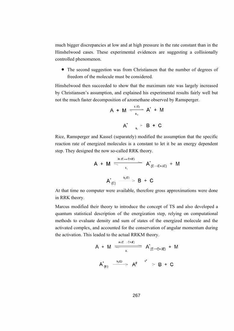
267

much bigger discrepancies at low and at high pressure in the rate constant than in the Hinshelwood cases. These experimental evidences are suggesting a collisionally controlled phenomenon.

The second suggestion was from Christiansen that the number of degrees of freedom of the molecule must be considered.

Hinshelwood then succeeded to show that the maximum rate was largely increased by Christiansen’s assumption, and explained his experimental results fairly well but not the much faster decomposition of azomethane observed by Ramsperger.

Rice, Ramsperger and Kassel (separately) modified the assumption that the specific reaction rate of energized molecules is a constant to let it be an energy dependent step. They designed the now so-called RRK theory.

At that time no computer were available, therefore gross approximations were done in RRK theory.

Marcus modified their theory to introduce the concept of TS and also developed a quantum statistical description of the energization step, relying on computational methods to evaluate density and sum of states of the energized molecule and the activated complex, and accounted for the conservation of angular momentum during the activation. This leaded to the actual RRKM theory.

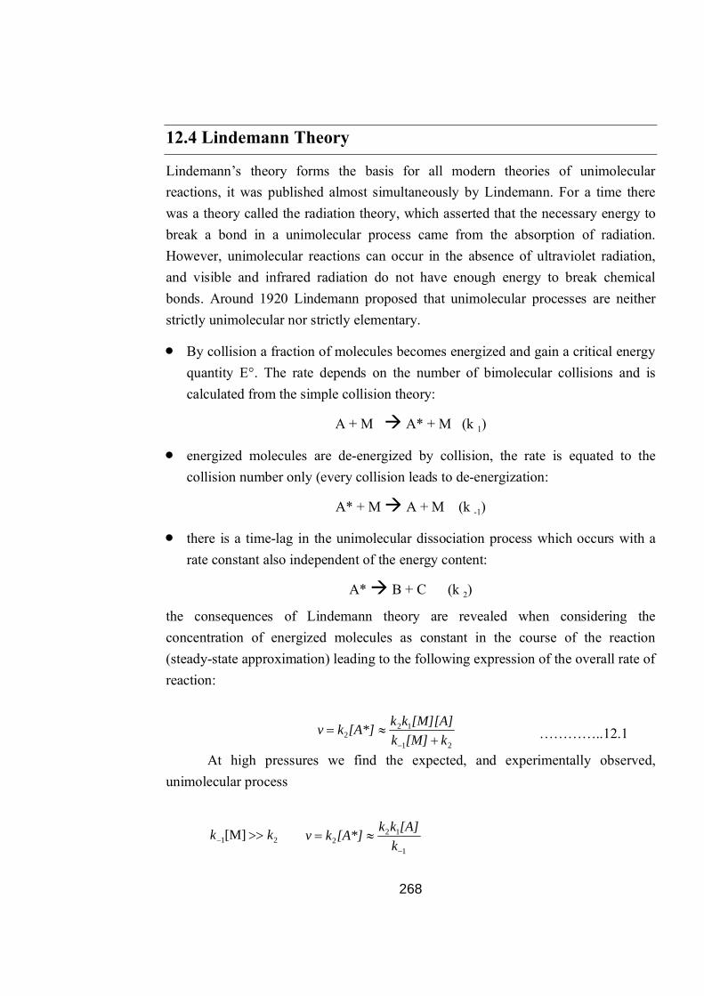
268

12.4 Lindemann Theory

Lindemann’s theory forms the basis for all modern theories of unimolecular reactions, it was published almost simultaneously by Lindemann. For a time there was a theory called the radiation theory, which asserted that the necessary energy to break a bond in a unimolecular process came from the absorption of radiation. However, unimolecular reactions can occur in the absence of ultraviolet radiation, and visible and infrared radiation do not have enough energy to break chemical bonds. Around 1920 Lindemann proposed that unimolecular processes are neither strictly unimolecular nor strictly elementary.

By collision a fraction of molecules becomes energized and gain a critical energy quantity E°. The rate depends on the number of bimolecular collisions and is calculated from the simple collision theory:

A + M A* + M (k 1)

energized molecules are de-energized by collision, the rate is equated to the collision number only (every collision leads to de-energization:

A* + M A + M (k -1)

there is a time-lag in the unimolecular dissociation process which occurs with a rate constant also independent of the energy content:

A* B + C (k 2)

the consequences of Lindemann theory are revealed when considering the concentration of energized molecules as constant in the course of the reaction (steady-state approximation) leading to the following expression of the overall rate of reaction:

…………..12.1

At high pressures we find the expected, and experimentally observed, unimolecular process

21

122 k[M]k

[M][A]kk[A*]kv

1

122

k

[A]kk[A*]kv21[M] kk

269

And at low pressures the reaction rate is then better described by a second order reaction:

This theory correctly predicts the rate constant fall-off at low pressures, but the values calculated are far from experimental results.

We can calculate the pressure at which the rate constant reaches half of its high pressure value (transition pressure): (Fig. 12.1)

Fig. 12.1 :mGrah between Log k v/S Lon [M]

where [M]1/2 is the “third body” concentration at which the experimental rate constant falls to half of its high pressure value.

Since no values for k2 could be provided by the theory, kinf was measured and k2 derived from it. The goal was then to get good agreement for the transition pressure. But problems arose with experimental values of [M]1/2, discrepancies between

[M]12 kk [A][M]k[A*]kv 12

M

M

12/1[M]

kk

1

12k

kkk

11/2[M]

kk

2]

22/11

2/112 kk[M]k

[Mkk

270

experimental and calculated values can be as big as 108, especially for bigger molecules.

It is usually called the first failure in Lindemann mechanism.

By considering the activation energy to be constant, and the collision frequency to be the same in all steps, we can modify the following equation:

……………..(12.5)

which is actually contradictory with the time-lag concept introduced to consider the unimolecular step.

This is what made Hinshelwood try to modify this theory and especially the expression of the activation rate to account for a longer lifetime of the energized molecule depending on the number of degrees of freedom

Lindemann mechanism in brief

the reaction occur in two steps, a bimolecular activation step and a unimolecular dissociation step.

all the rate constants are independent of the internal energy of the molecules.

the rate of energization is calculated on the basis of SCT.

the rate of de-energization is simply the collision frequency (strong collision).

the unimolecular step is said to be rate determining at high pressure and a fast step at low pressure.

there are evident two failures:

the fall-off critical region is not well-described (discrepancies between theoretical data and experimental data diverge with molecules getting bigger).

the linear extrapolation of inverse plot expected is not found experimentally (low pressure description not correct, modification of bimolecular step description).

1

12 k

kkk

271

12.5 Hinshelwood theory

Accounting for suggestions made by Christiansen and Lindemann, Hinshelwood modified the previous mechanism to account for internal degrees of freedom during the activation process. He then modeled the internal modes of A by a hypothetical molecule having s equivalent classical harmonic oscillators, and by considering thermal equilibrium and the strong collision assumption (meaning that the probability of deactivation is equal to the collision frequency, each collision is efficient to deactivate), he obtained:

since TkE B0 the new factor in the expression of the rate constant is very much greater than unity, which is giving a higher rate constant for larger molecules and is exactly what is required to overcome the problem with the too short time-lag in the unimolecular step.

Satisfactory fits to experimental data could always be done with this theory at the transition pressure but not on the whole range of pressure (cis -> trans-but-2-ene):

2

Fig. 12.2 Graph for theositical and expoimental data

TkE

TkE

sZk

B

s

B

01

01 exp

)!1(

272

Moreover the fits were always obtained by considering a number of degrees of freedom different to the one expected for the molecule, without a priori method of calculation of s for a particular reaction. (Fig. 12.2)

12.6 RRK theory

Rice and Ramsperger and Kassel who introduced a quantum formulation of the theory, recognized that the rate of the unimolecular step should depend on the vibrational energy of the energized molecule as well. For that purpose, they had given the idea that a minimum of energy must be localized in specific modes of molecular motion in order for the dissociation to take place, and that the newly calculated rate constant must be proportional to that probability.

They did not mention an activated complex intermediate but instead considered the energy localization process to compute the rate constant.

They kept the Hinshelwood-Lindemann theory in its state and modified the expression of the unimolecular step to account for their new idea. They started by considering that energy can flow freely among the different oscillators, then Kassel (in its quantum calculations) computed the number of ways to distribute )( m quanta over the s oscillators (since m quanta will be located on the critical oscillator) to get:

……………..(12.7)


……………..(12.8)

Considering the classical limit which consists in having a very large number of quanta compare to the number of oscillators, Kassel got:

)!1()!()!1(!

sm

smPm

)!1()!()!1(

smsm

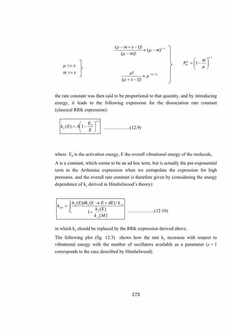
273


……………..(12.9)

where E0 is the activation energy, E the overall vibrational energy of the molecule,

A is a constant, which seems to be an ad hoc term, but is actually the pre-exponential term in the Arrhenius expression when we extrapolate the expression for high pressures. and the overall rate constant is therefore given by (considering the energy dependence of k1 derived in Hinshelwood’s theory):

……………..(12.10)


The following plot (fig. 12.3) shows how the rate k2 increases with respect to vibrational energy with the number of oscillators available as a parameter (s = 1 corresponds to the case described by Hinshelwood).

1

1

s

mmP

10

2 1)(

s

EEAEk

sms

1)()!(

)!1(

smmsm

)1(

)!1(!

s

s

0

][)(1

/)()(

1

2

112

Euni

MkEk

kdEEEdkEkk

274

Fig. 12.3 : Graph between rate and vibrational energy

which is actually exactly what we need to have a better description at low pressure.

Although Kassel’s theory was giving better agreement to experiments, gross approximations were made leading to results for which the number of oscillators couldn’t be predicted a priori.


a) Lindemann theory form basis of ………..reactions.

b) Energized molecules are de energized by ……………

c) According to lindermann theory. At low peruse rate follow …………….order

kidtees.

d) Hinshefrood consider …………..along with anti vation process.

12.7 RRKM theory

The RRK theory was an important development in the treatment of unimolecular reactions, but gross approximations were made at that time due to a lack of computational methods. Marcus, with Rice’s help, developed the now called RRKM theory in 1952. Its main new features with respect to RRK are as follows:

The time required for dissociation is long relative to the time required for ion formation/excitation/activation.

275

The time required for dissociation is long relative to the time required for redistribution of energy over all internal modes of the ion (ergodicity, energy can slosh around) and the distribution of reactants is defined by a microcanonical ensemble i. e. RRKM does not apply to non-ergodic processes such as ECD/ETD.

The reaction is adiabatic; it takes place on a single potential energy surface, upon which the motion is classical, that links reactants to products and is separable from the other molecular motions.

The products observed are from competing and consecutive reactions.

There is a unique dividing surface (T.S.) which divides the reactants from the products which is a point of no return

The energization rate constant k1 is evaluated as a function of energy by quantum-statistical mechanical treatment.

It considers explicitly the concept of Transition State in the unimolecular process as an intermediate step (and converges to ART at the high pressure limit) and deals with the real frequencies of the energized molecule as well as of the TS, and treats explicitly the rotational degrees of freedom in the course of the dissociation.




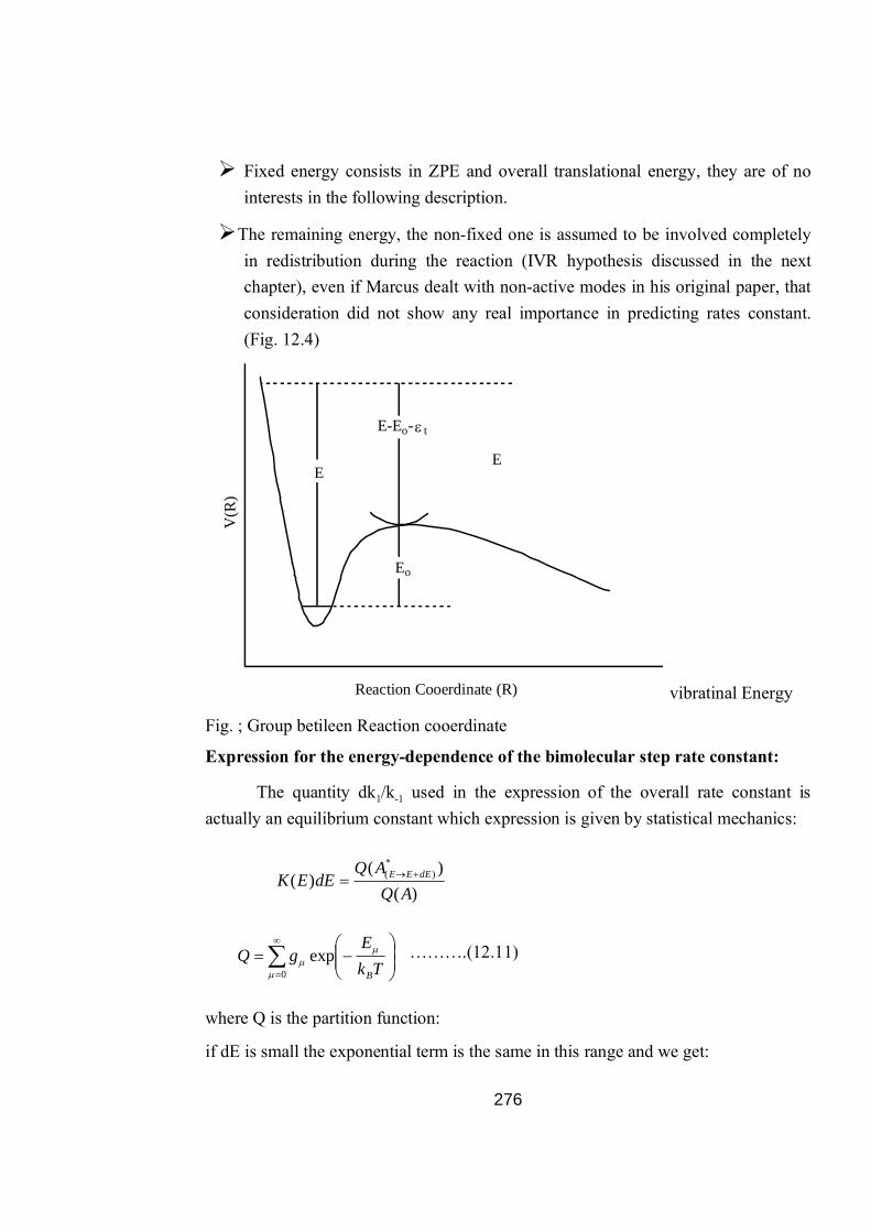
276

Fixed energy consists in ZPE and overall translational energy, they are of no interests in the following description.

The remaining energy, the non-fixed one is assumed to be involved completely in redistribution during the reaction (IVR hypothesis discussed in the next chapter), even if Marcus dealt with non-active modes in his original paper, that consideration did not show any real importance in predicting rates constant. (Fig. 12.4)

E-Eo- t

Eo

EE

Reaction Cooerdinate (R)

V(R

)

vibratinal Energy

Fig. ; Group betileen Reaction cooerdinate

Expression for the energy-dependence of the bimolecular step rate constant:

The quantity dk1/k-1 used in the expression of the overall rate constant is actually an equilibrium constant which expression is given by statistical mechanics:

……….(12.11)

where Q is the partition function:

if dE is small the exponential term is the same in this range and we get:

0exp

Tk

EgQ

B

)()(

)(*

)(

AQAQ

dEEK dEEE

277

……….(12.13)

and finally:

……….(12.14)

which is in fact the quantum Boltzmann distribution giving the thermal equilibrium proportion of molecules in the given energy range.

Expression for the energy dependence of the dissociation step


we get: ][][

21)( *2 A

AkEk

……………….(12.15)


……………….(12.16)

with x the translational energy of the molecule at the top of the barrier, m its mass, and the length of the “box”

Considering again the two species to be at thermal equilibrium, the ratio of their concentrations is then expressed as the ratio of their partition function (they have the same ground state energy), both these species have the total energy in the same range

dEEE and the ratio of their partition function reduces to the ratio of the sum of

Tk

EdEETk

EgAQBB

dEEE exp.)(exp.)(0

*

TkE

AQdEE

AQAQ

kdEEEdk

B

dEEE exp.)(

)()(

)()( *)(

2

1

2/1

22

mxk

278

the degeneracies, which at the energy of interest, chemical energies, can be approximated by the ratio of their density of states:

……………….(12.17)


By using the expression of the number of states given in our lecture on TST, and by considering all the calculated expression, we get the for the activation rate constant:

……………….(12.18)


Another point has been omitted, is the problem of multiple reaction paths. The example of dissociation of H2O leads to two equivalent paths, and to account for that we should include another factor called statistical factor or reaction path degeneracy L#.


……………………….(12.19)


)()()(

][][

*** ExNEP

AA

eq

E

E

EPEh

Ek0

'**2

'

)()(

1)(

E

E

EPEhQ

QLEk0

'**

1

12

'

)()(

1)(

279

Approximations in RRKM

(A) Intramolecular Vibrational Relaxation


As mentioned previously, Marcus made provision for some of the degrees of freedom to be completely inactive and which could therefore not participate to the dissociation process. This energy can however be redistributed randomly between these modes and affects the density of states of the energized molecule as well as the activation rate constant.

There is little evidence that energy is rapidly redistributed between all vibrational modes involved within a time not greater than 10-11 s.

(B) Strong collisions assumption

This assumption means that relatively large amounts of energy are transferred in molecular collisions (>> kT). RRKM assumes then the energization step to be single-step on contrary to ladder-climbing processes. This assumption also assumes that the molecule after collision is in a state completely independent as the one before, no dynamical details of the collision are thus necessary within that description.

A more detailed study of energization step can be done involving accurate description of the dynamics of collision, and it seems relatively important for small molecules.

(C) The equilibrium hypothesis

In the unimolecular step it was assumed as in ART that the TS is crossed as if there would be equilibrium between energized and activated molecules (SSA as if no net reaction is occurring, total equilibrium of reverse reaction).


(D) Continuous distribution function of state density

The approximation of continuous density of states for the activated complex can be cumbersome, since most of the energy available is fixed to overcome the barrier and

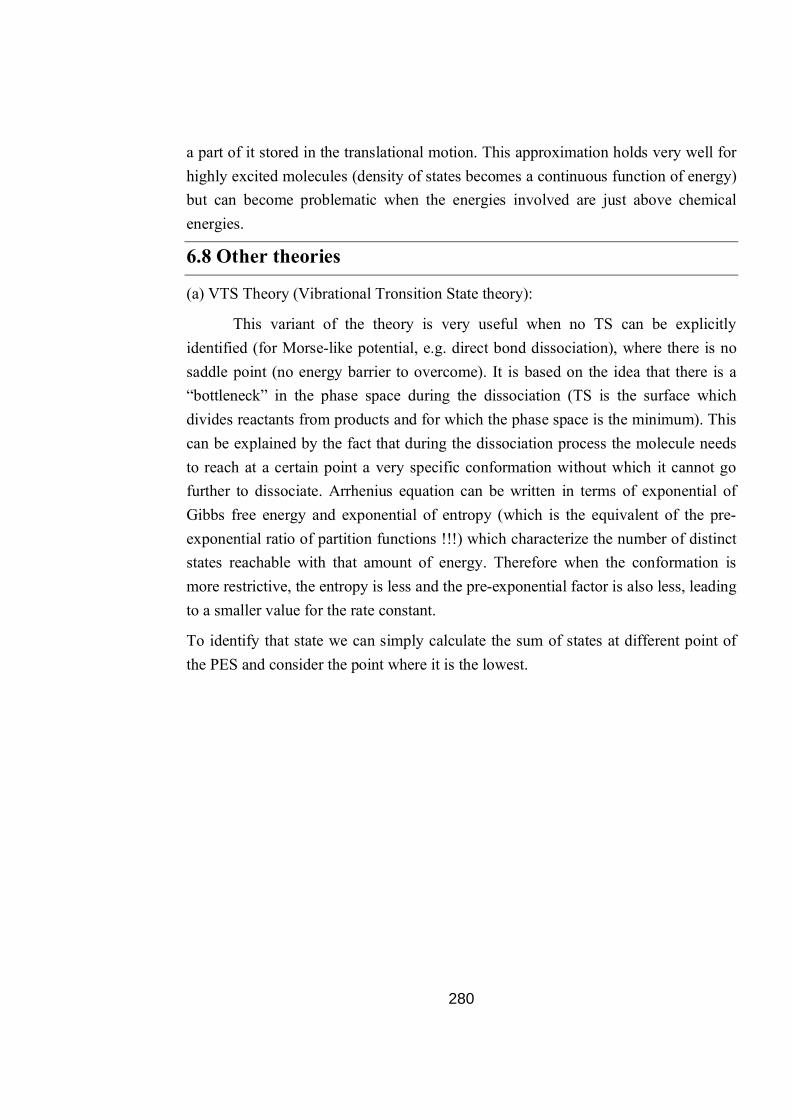
280

a part of it stored in the translational motion. This approximation holds very well for highly excited molecules (density of states becomes a continuous function of energy) but can become problematic when the energies involved are just above chemical energies.

6.8 Other theories

(a) VTS Theory (Vibrational Tronsition State theory):

This variant of the theory is very useful when no TS can be explicitly identified (for Morse-like potential, e.g. direct bond dissociation), where there is no saddle point (no energy barrier to overcome). It is based on the idea that there is a “bottleneck” in the phase space during the dissociation (TS is the surface which divides reactants from products and for which the phase space is the minimum). This can be explained by the fact that during the dissociation process the molecule needs to reach at a certain point a very specific conformation without which it cannot go further to dissociate. Arrhenius equation can be written in terms of exponential of Gibbs free energy and exponential of entropy (which is the equivalent of the pre-exponential ratio of partition functions !!!) which characterize the number of distinct states reachable with that amount of energy. Therefore when the conformation is more restrictive, the entropy is less and the pre-exponential factor is also less, leading to a smaller value for the rate constant.

To identify that state we can simply calculate the sum of states at different point of the PES and consider the point where it is the lowest.

281

This is the idea of VTST This type of calculations can be performed with the help of the software.

(b) Phase Space theory:

The statistical dissociation rate constant can be calculated from the point of view of the reverse reaction. Again this procedure is limited to reaction without energy barrier (called loose TS reaction).

It is considering that the decomposition is governed only by the phase space available under strict energy and angular momentum conservation. Considering equilibrium between reactants and products, we get:

………………(12.20)

for which there is no need of informations on the TS.

),(),(),(

][]][[ 00

JEjEEjEEkk

ABBA

kk

AB

BAbimuni

bim

uni

282

12.2 state True false

a) Adiabatic reaction takes place on a single potential energy surface (T/F).

b) Energy does not flow freely among different modes of molecules before it can

dissociate (T/F).

c) After collision molecule is in completely independent state

d) Vibration transition state theory is useful when no transition state is identified

(T/F).

12.9 Summary

This chapter discusses the following topics:

Basic concept of unimolecular reactions,

Lindemann theory of unimolecular reactions and its failures,

Hinshelwood and RRK theory,

RRKM theory and its approximations and some other theories

12.10 Glossary





283




12.1 a) unimeladular b) Callician c) seemond d) degree of freedom12.2 a) T b) F

c) T d) T


1. What are unimoleculre reactions? Explain with examples. 2. Write short note on theories of unimoleculre reaction rates. 3. Give Lindemann theory for unimoleculre reaction rates. 4. What are the evidences of failures of Lindemann theory. 5. Write detailed notes on Hinshelwood and RRKM theory. 6. Discuss RRKM theory in detail.





284

Unit- 13 : Statistical Thermodynamics Structure of Unit

13.0 Objectives

13.1 Introduction

13.2 Some Statistics Necessities

13.3 Probability of Sytem

13.4 Phase Space

13.5 Microstate and Macrostate

13.6 Thermo dynamic Probability

13.7 System, assembly and Ensembles

13.8 Uniform and micro connonical enemble

13.9 Cannonical ensembles

13.10 Grand cannonical ensemsbles

13.11 Significance of ensembles

13.12 Sum marry

13.13 Glossary

Answer tk key assessment questions



13.0 Objectives At the end of the chapter the student will able :-

To understand various probability therms.

To define phase space, occupation number, dutribustion.

To differentiate between micro state and macro state

To undrestand the concept of thermo dynamic probability.

To derive condition of maximum probability.

To know about modifications in probability equation.

To differentrate between different types of ensembles

285

To give understand significance of ensembles

13.1 Introduction Various physical chemist investigate a wide variety of process of involving micro scopic systems consisting of isolated atoms and molecules. They also studied macroscopic systems consisting of large collection of particles at other hand. So there comes Statistical thermo dynamics which relate the properties of microscopic and macro scopic system to make fundamentals of physical chemistry. In this chapter we will consider the energies of individual atoms and moleules and the statistical theroy that relate them to macroscopic properties. Stastical thermodynanmies can be used for systems at equilibrium as well as away from equilibrium. It acts as a bridge between thermodynamic and quantum chemistry. It also deals with relationship between the probability partition functions and thermodynamic properties and ensembles.

13.1 Fill in the blanks.

2 In ground can logical ensemble T,V and ________ remain content.

3 Micro can logical ensemble describes an ___________ system.

4 Microcanlogical ensemble desirables an __________V, and number.

5 Same, E,V, and N are found in ___________ensambles.

6 Total number of micro state by which given macro state is defred is

__________.

7 The number of ways in which N distinguishable particulars be arranged

will be equal to _______________.

8 The six dimensional space is called.________________.

13.2 Some Statistics Necossities In order to understand statistical thermodynamic, it is necessary to generalize some statistical ideas Consider a system that is composed of three boxes that represent smaller subsystems. Now we can determine that in how many ways a single block ball be places into three identical but seperate boxes ? (Fig 13.1)

286

Fig 13.1 : Three ways of Putting single ball

Now let us suppose we have a black and a white ball to be distributed in three identical boxes. Because the balls are different, the possible arrangements for our distribution are different than if the balls are identical. There are six possibilities.

The two different types of same and different colored ball illustrate the concepts of distiginshable versus inditinguishable objects. When the desired objects that are being partitioned into seperate subsequents are distinguishable, there are more possible ways of amanging the objects in the subsystem. As compared if the object are indistingawishable, there are fever unique ways. We can express the population of boxes in terms of probalitities.

13.3 Probability of System We consider a closed system composed of N molecules although the thotal energy is constant E, it is not possible to define that how that energy is shared between the molecules. The closest we can come to a description of the distribution of energy is to report the population of state, the average number of molecules that occupy is. The population of the states remain almost concstant but the precive identities of the molecules in each state may change at every collision. The following are the important probability theorms which are commonly used in statistical thermodynamics:-

1. The number of ways in which N distinguishable particles can be areranged in order will be equal to N!

2. The number of different ways in which n particles can selected from N distinguishable particles irrespective of the order of selection will be equal to

!( )! !

NN n n

287

3. The number of different ways in which n indistinguishable particles can be arranged in g distinguishable states with not more than one paticles in each state will be equal to

!!( )!

gn g n

In general probability of an event = Number of casesin which theevent occurs

Total Number of cases 13.4 Phase Space

The state of a gas can be specified by defining the state of each moecule of the gas. The state of each molecules can be specified by defining its position and momentum. That means we must specify x,y,z, and Px, Py, Pz for each of the molecules. The intire phase space is divided into number of very small elements of volume. An element of volume in a space is termed as cell or unit cell.

In three dimensional space, we can easily consider on element of volume dx, dy, dz. We can plot momentum px, py, pz in three mutually perpendicular directions and again consider three dimensional volume dpx, dpy and dpz. So we can imagine a six dimensional space in which dx, dy, dz, dpx, dpy, dpz is an element of volume and posiston. This six dimensional space is called phase space and an element of volume in space is term as cell. We can also define occupation number in phase as the number of systems in that particular state. The set of occupation numbers is called a distribution.

13.5 Micro State and Macro State Let us divide the phase space into cell numbered 1,2,3.... etc. The micro state of the system may be defined by the specification of six co-ordinates x,y,z and px,py,pz of each molecules of the system with in the limits of the dimensions of the cell in which its representative point lies.

In order to define micro state we must specify the place of each molecule with the limits dx, dy, dz and the magnitude and direction of each molecule with the limits dpx, dpy and dpz. We can also say it a way, that in order to define a micro state we must mention to which the cell of each molecule of the system belongs temporarily.

A macro state of the system may be defined by the specification of the number of molecules or phase points in each cell of phase space. For eg.m1 molecules in cell m1,

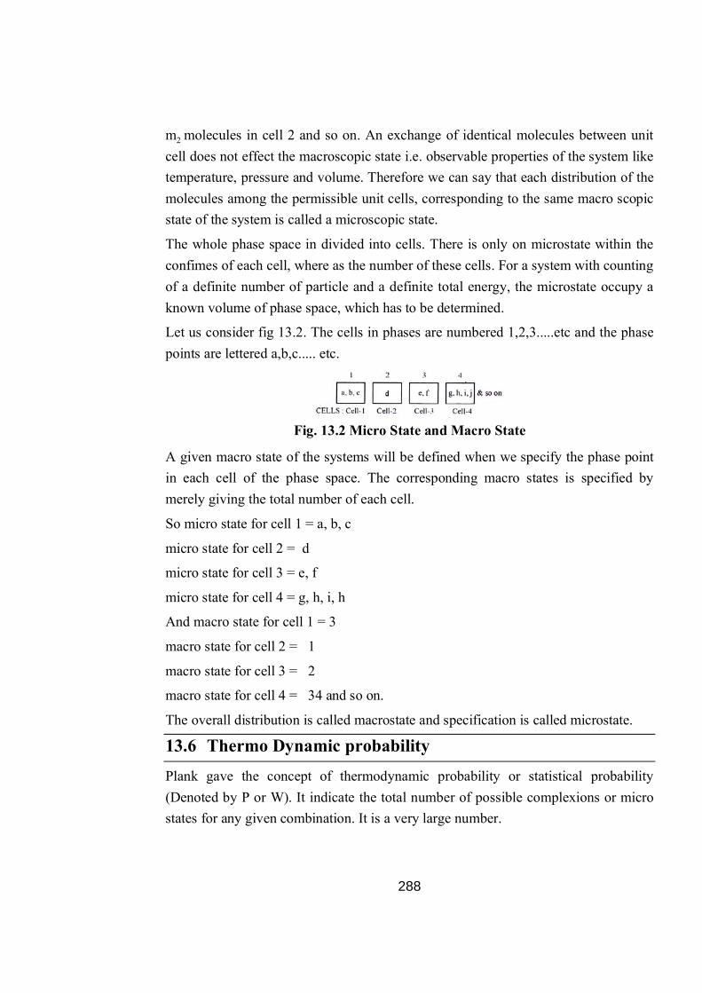
288

m2 molecules in cell 2 and so on. An exchange of identical molecules between unit cell does not effect the macroscopic state i.e. observable properties of the system like temperature, pressure and volume. Therefore we can say that each distribution of the molecules among the permissible unit cells, corresponding to the same macro scopic state of the system is called a microscopic state.

The whole phase space in divided into cells. There is only on microstate within the confimes of each cell, where as the number of these cells. For a system with counting of a definite number of particle and a definite total energy, the microstate occupy a known volume of phase space, which has to be determined.

Let us consider fig 13.2. The cells in phases are numbered 1,2,3.....etc and the phase points are lettered a,b,c..... etc.

Fig. 13.2 Micro State and Macro State

A given macro state of the systems will be defined when we specify the phase point in each cell of the phase space. The corresponding macro states is specified by merely giving the total number of each cell.

So micro state for cell 1 = a, b, c

micro state for cell 2 = d

micro state for cell 3 = e, f

micro state for cell 4 = g, h, i, h

And macro state for cell 1 = 3

macro state for cell 2 = 1

macro state for cell 3 = 2

macro state for cell 4 = 34 and so on.

The overall distribution is called macrostate and specification is called microstate.

13.6 Thermo Dynamic probability Plank gave the concept of thermodynamic probability or statistical probability (Denoted by P or W). It indicate the total number of possible complexions or micro states for any given combination. It is a very large number.

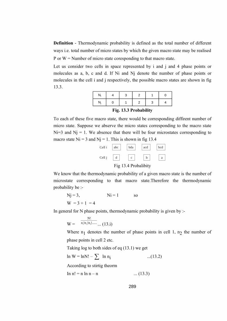
289

Definition - Thermodynamic probability is defined as the total number of different ways i.e. total number of micro states by which the given macro state may be realised

P or W = Number of micro state coresponding to that macro state.

Let us consider two cells in space represented by i and j and 4 phase points or molecules as a, b, c and d. If Ni and Nj denote the number of phase points or molecules in the cell i and j respectively, the possible macro states are shown in fig 13.3.

Ni 4 3 2 1 0

Nj 0 1 2 3 4 Fig. 13.3 Probability

To each of these five macro state, there would be corresponding diffirent number of micro state. Suppose we abserve the micro states corresponding to the macro state Ni=3 and Nj = 1. We absence that there will be four microstates corresponding to macro state Ni = 3 and Nj = 1. This is shown in fig 13.4

abc bda acd bcd

d c b a

Cell i

Cell j Fig 13.4 Probalibity

We know that the thermodynamic probability of a given macro state is the number of microstate corresponding to that macro state.Therefore the thermodynamic probability be :-

Nj = 3, Ni = 1 so

W = 3 + 1 = 4

In general for N phase points, thermodynamic probability is given by :-

W = 1 2 3

N!n !n !n !...... ... (13.i)

Where n1 denotes the number of phase points in cell 1, n2 the number of

phase points in cell 2 etc.

Taking log to both sides of eq (13.1) we get

ln W = lnN! – ln ni ...(13.2)

According to stirtig theorm

In n! = n ln n – n ... (13.3)

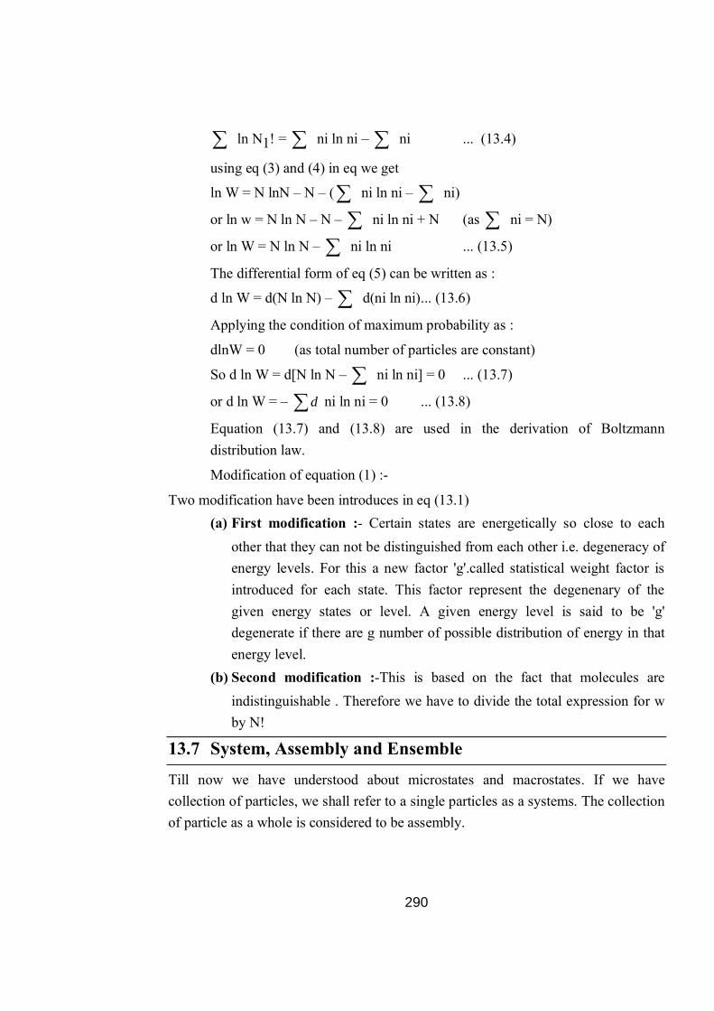
290

ln N1! = ni ln ni – ni ... (13.4)

using eq (3) and (4) in eq we get

ln W = N lnN – N – ( ni ln ni – ni)

or ln w = N ln N – N – ni ln ni + N (as ni = N)

or ln W = N ln N – ni ln ni ... (13.5)

The differential form of eq (5) can be written as :

d ln W = d(N ln N) – d(ni ln ni)... (13.6)

Applying the condition of maximum probability as :

dlnW = 0 (as total number of particles are constant)

So d ln W = d[N ln N – ni ln ni] = 0 ... (13.7)

or d ln W = – d ni ln ni = 0 ... (13.8)

Equation (13.7) and (13.8) are used in the derivation of Boltzmann distribution law.

Modification of equation (1) :-

Two modification have been introduces in eq (13.1) (a) First modification :- Certain states are energetically so close to each

other that they can not be distinguished from each other i.e. degeneracy of energy levels. For this a new factor 'g'.called statistical weight factor is introduced for each state. This factor represent the degenenary of the given energy states or level. A given energy level is said to be 'g' degenerate if there are g number of possible distribution of energy in that energy level.

(b) Second modification :-This is based on the fact that molecules are indistinguishable . Therefore we have to divide the total expression for w by N!

13.7 System, Assembly and Ensemble

Till now we have understood about microstates and macrostates. If we have collection of particles, we shall refer to a single particles as a systems. The collection of particle as a whole is considered to be assembly.

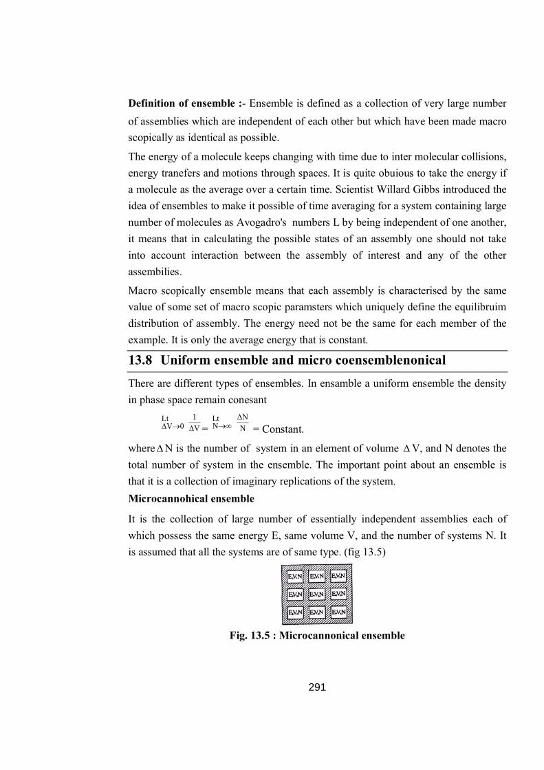
291

Definition of ensemble :- Ensemble is defined as a collection of very large number of assemblies which are independent of each other but which have been made macro scopically as identical as possible.

The energy of a molecule keeps changing with time due to inter molecular collisions, energy tranefers and motions through spaces. It is quite obuious to take the energy if a molecule as the average over a certain time. Scientist Willard Gibbs introduced the idea of ensembles to make it possible of time averaging for a system containing large number of molecules as Avogadro's numbers L by being independent of one another, it means that in calculating the possible states of an assembly one should not take into account interaction between the assembly of interest and any of the other assembilies.

Macro scopically ensemble means that each assembly is characterised by the same value of some set of macro scopic paramsters which uniquely define the equilibruim distribution of assembly. The energy need not be the same for each member of the example. It is only the average energy that is constant.

13.8 Uniform ensemble and micro coensemblenonical There are different types of ensembles. In ensamble a uniform ensemble the density in phase space remain conesant

1Lt

ΔV 0 ΔV = ΔNLt

N N = Constant.

whereN is the number of system in an element of volume V, and N denotes the total number of system in the ensemble. The important point about an ensemble is that it is a collection of imaginary replications of the system. Microcannohical ensemble

It is the collection of large number of essentially independent assemblies each of which possess the same energy E, same volume V, and the number of systems N. It is assumed that all the systems are of same type. (fig 13.5)

Fig. 13.5 : Microcannonical ensemble

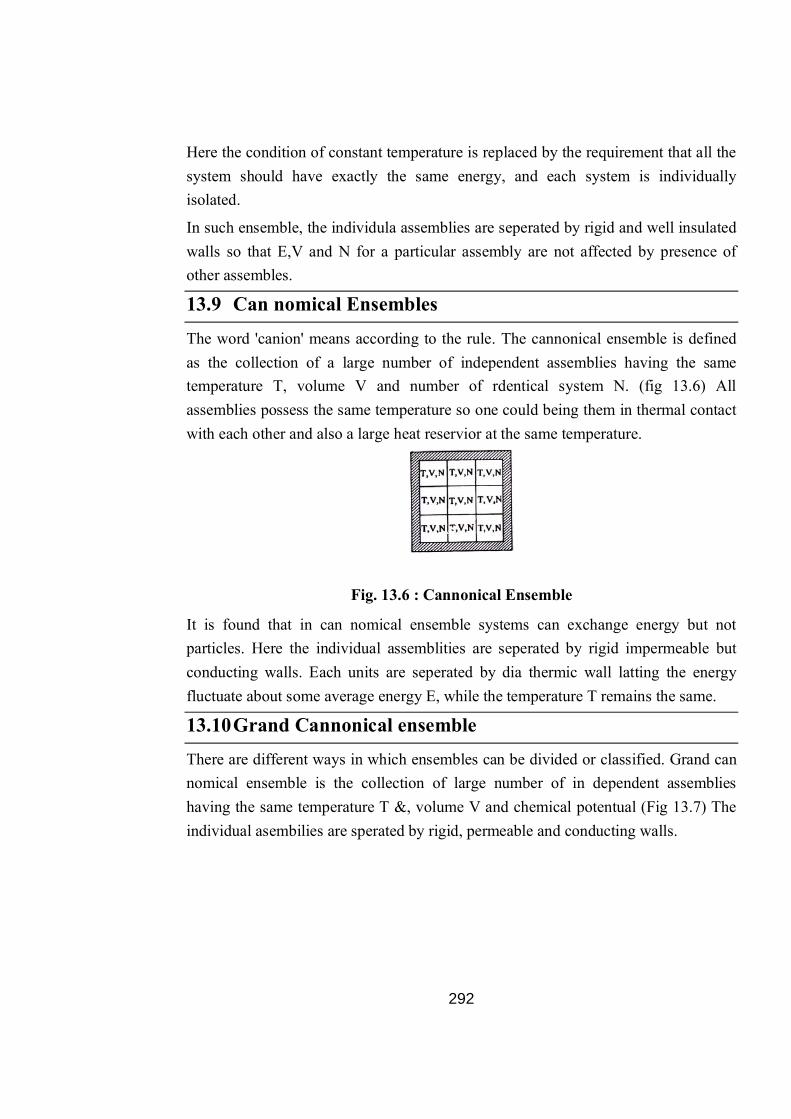
292

Here the condition of constant temperature is replaced by the requirement that all the system should have exactly the same energy, and each system is individually isolated.

In such ensemble, the individula assemblies are seperated by rigid and well insulated walls so that E,V and N for a particular assembly are not affected by presence of other assembles.

13.9 Can nomical Ensembles

The word 'canion' means according to the rule. The cannonical ensemble is defined as the collection of a large number of independent assemblies having the same temperature T, volume V and number of rdentical system N. (fig 13.6) All assemblies possess the same temperature so one could being them in thermal contact with each other and also a large heat reservior at the same temperature.

Fig. 13.6 : Cannonical Ensemble

It is found that in can nomical ensemble systems can exchange energy but not particles. Here the individual assemblities are seperated by rigid impermeable but conducting walls. Each units are seperated by dia thermic wall latting the energy fluctuate about some average energy E, while the temperature T remains the same.

13.10 Grand Cannonical ensemble There are different ways in which ensembles can be divided or classified. Grand can nomical ensemble is the collection of large number of in dependent assemblies having the same temperature T &, volume V and chemical potentual (Fig 13.7) The individual asembilies are sperated by rigid, permeable and conducting walls.

293

Fig. 13.7 : Grand Cannonical ensemble

Each assemblies can exchange both energy as well as particles with one another. The thermodynamic variables of the grand cannonical ensembles are absolute temperature and chemical potential.

It is exactly the ensemble that describes the possible states of an isolated systems that is in thermal and chemical equiliburim with a reservifour. The grand cannonical ensemble applies exactly to systems of any size, white it is necessary to assume that the reservior is vary large (i.e. in the macro scopic limit) the system it self may be small or large. Properties

1. It is uniquely determined for a given system at a given temperature and given chemical poetentials.

2. It does not evolve over time ,as it is a function of conserved quantities.

13.11 Significance of ensembles 1. The grand cannonical ensemble is uniquely determined for a given system

at given temperature and given chemical potential.

2. Ensemble is only a function of a conserved quantities of the system.

3. Micro cannomical ensemble describes an isolated system.

4. Cannonical ensemble describes a system in contact with heat bath.

5. Grand cannonical ensemble describe a system in contact with heat and particle bath.

6. They are used to relate micro states to macro states for a particular system.

7. They describe the statistical distribution of a system.

8. Each member of cannonical ensemble can be confired with the heat bath to become a member of a micro can nonical ensemble.

294

13.12 Summary

Statistical thermo dynamics is a branch of science which deals with micro scopic and macro scopic properties of a system.

Their are different prabilities theorm theams by which particles can be distributed.

The six dimensional space is called phase space and an element of volume in space is called cell.

Thermodynamic probabilities is the total number of positive complexions or micro states for a given combination.

In uniform ensemble the density in phase space remain constant.

In micro cannonical ensemble energy, volume and number of system remain constant.

In cannonical ensemble temperature, volume and number of identical system remain constant.

In grand cannonical ensemble temperature, volume and chemical potential remain constant.

13.13 Glossory

Phase space: -- six dimensional state (Px,PY, Pz,dx, dz) .

Occupation number :-- number of system in that particular

Macro state: -- specification of the number of molecules.

Micro state:-- specification of six coordinative.

Ensemble: - Collection of large number of assemblies which are independent

of each other.


13.1 a) Chemical Potential b) liolated c) T d) micro chemical (e) Thermodynamic

Probalility f) N ! g) Phase shape

295

13.14 Review question A) Short Answer type

1. Difine statitiscal thermo dynamic

2. What do you mean by probability of system?

3. Give different ways by which N distinguishable particles can be arranged?

4. Define phase space and occupation number?

5. Defferentiate between micro state and macro state

6. State thermo dynamic probability?

7. What do you understand by system and assembly? B) Long Anser type

1. What do you mean by ensembles? What are different types of ensembles.

2. Differntreiate between micro cannonical and grand can nonical ensembles.

3. What do you mean by micro and macro state of system. How particles are distributed in them?

4. What do you understand by grand cannonical ensembles? Give significance of ensembles also.

5. What is thermodynamic probability? How stirling formula is used in its determination.

6. What is the importane of phase space in stistical thermo dynamics? Also give different types of ensembles and their properties.


2. Physical chemistry - Peter Atkins, Julio de Paula

3. Physical chemistry - Clyde R. Metz

4. Physical chemistry - Puri Sharma, Pathania


6. Advanced physical chemistry - J.N. Gurtu and A Gurtu

296

Unit - 14 : Partition Function Structure of Unit

14.0 Objective

14.1 Introduction

14.2 Partition function

14.3 Significance

14.4 transelational partition function

14.5 Retational partition function

14.6 Vibrational partition function

14.7 Electronic partition function

14.8 Molar partition function

14.9 Summary

14.10 Glossary



14.12 Refernce and suggested readings

14.0 Objectives At the end of this chapter sutdent will able -

To define partition function

To give significance of partition function

To state transelational position function

To difine translational part function in three directions

To explore devivation fo rotational par for

To konw retational part fun for polyatomic molewles

To understand electrics part fun

To suggest wbrationat part function and its devivation

To give relationship between molar part fun and molecular part function.

297

14.1 Introduction Till now we have read some thing about statitical thermo dynamics. It is a branch which deals with relationship between micro states to macro states. Their are variuos terms unvalue in it and different types of statistics like Maxwall Boltzmann distribution law. Fermi Diar statistics and Bose Einesterm law. All these are their in next unit. Here we will going to understane the meaning of partition function, different types of partitions function and also their specific derivation we are also able to understand the significance of partition function.

14.2 Partition function Defination

The term partition function is given by formula. It is a dismensionaless quantity. Its value depend on the molecular weight, mlecular volume and temperature. It is defined as sum of the probability factor for different energy states or as the way in which the energy of a system partitional among the moleculas constituting the system. It can be symbolized as Q.

–Ei/KTQ = Σgie ... (14.1)

Where gi is the statistical weight factor and is equal to degree of degenerary. It can be defmed as number of superiparsed energy level, K is Boltzmann constant and Ei is the energy of quantum state, and T is the temperature is caluin seale.

In above equation summation is taken over all integral of i from zero to infinity concsponding to all possible energy states of the molecule. Therefor equation (14.1) becomes as

0

–Ei/KT

i=0Q = gie

... (14.2)

The contribution of Ei for an ideal gas are nurlear electronic, bibrational, rotational an translational. That means above equation can be metters as :-

Ei = Enue + Eelr + EVib + Erot + Etrans ... (14.3)

With the help of partition function we can relate macro scopic properties of individula molecules.

14.3 Significance Statistical thermodynamics analysis is farilitated through the use of partition function. It is a very important analytical tool.

298

1. In terms of language it is the way in which the energy of a system of molecules is partitioned among the molecular inhabitants. It is a dimensionless quantity.

2. Its value depend on various factor s like molecular weight, the temperature, molecular volume, the inter nuclear distances, the molecular motions and intermatacular forces.

3. It provide a way by means of which we can link the micro scopic properties of individual molecular. We can relate their discrete energy levels moment of inertia and depole momento to the macro scopic properties like molar heat, entropy and polarization

4. According to Maxwell Boltzmann law

–Ei/KTni gi= e

no go ... (14.4)

Wherer hi is number of molecules in ith state, no is number of molecules in zero state. The term gi and go represent degeneracies in respective level. When

E0 = 0, then g0 = 1, so e. (14.4) can be written

as –Ei/KTni = e

no

or ni = no gi e–Ei/KT ... (14.5)

Taking sum motion of above equation use get

ni = n0 gi E–Ei/KT

ni = n0 Q ... (14.6)

As ni = n

So n = n0Q

or Q = nn0 ... (14.7)

If we study equation (14.7) then use can difine partition function as reation of the number of particles is its level to that of zero level.At absolute zero.

T 0, n n0 and Q 1 ... (14.8)

It means value of partition function increases with temperature. As temperature increases there are few number of molecules is zero energy level and more molecules

299

in highest energy levels. So we can say that partition function is larger at higher temperature Q is also refered as molecular partition function.

14.4 Translational partition function The partition functino for translational motino is one direction is given Qt.

Qt(x) = –Et/KTgte

Where Qt (x) is translational partition function in x directio ; K Boltzmann constant. T is the temperatures and gt is the statistical weight of each translational level.

As statistical weight of each level is unity (gt=1), above eq (14.9) change to

Qt(x) = –Et/KTe ... (14.10)

Let us consider a cube of length l. The molecule moving along x axis will repeat its motinos each time on transwering a distance of 2l. Let is the wauelingth associated with the matter wave we have

n x = 2 x .... (14.11)

or x = x2

x

... (14.12)

We know that energy of such particle is

Et = 2Px

2m ... (14.13)

Where Px is the momentum of moving particle. We know that momentum is

Px = x

h or Px2 = 2

2

x

h ... (14.14)

Using (14.14) is eq (14.13) we get

Et = 2

2

x

h2m

Using eq (14.12) in above eq. we get -

Et = 2

2 2

x

h n2m(4 ) = ... (14.15)

So

2 2 2

( x )

–n h /8m xtQ e KT

... (14.16)

300

As the energy levels are so closely spared that the variation of energy may be taken to be continuous, for doing this we have to replace summation by integration so that equation (14.16) changes to

2 2 2

( x )

–n h /8m xt

0

Q e KT

dn

or , 2

( x)

–n at

0

Q e

dn .... (14.17)

2

2

hWherea8m x KT

from integral calculus use get

Or t1Q (x)2 a

2

t 2

1 8m x KTQ (x)2 h

1/ 22 mKT . x

h

= ... (14.18)

Translational partition function in three directions x,y,z at right angle to each other is given by -

Qt = Qt(x) .Qt(y).Qt(z)

=

3/ 2

x y z3

2 mKT .h

3/ 2

32 mKT .V

h

= .... (14.19)

when V is the volume accessible to molecule -

14.5 Rotational Partition Function The partition function for rotational energy of a diatomic molecule is given by following equation

–Br / KTr rQ g e ... (14.20)

Where Er.is rotational energy for deatomic molerule. The ratational energy according to quantum mehanis can be given by following equation.

2

r 2

hE J(J 1)8 I

... (14.21)

301

Where J is rotational quantum number and I is moment of Inertia.

We know that the rotational energy at the Jth level is degenerate is (2J+1) ways, so statistical

weight can be given by

gr = (2J + 1) ... (14.22)

Adding all the equation we get

2 2–J(J 1)h /8 IKT

rQ (2J 1)e ... (14.23)

Replacing summatin by integratin we get

2 2–J(J 1)h /8 IKT

r0

Q (2J 1)e

dJ

–J(J 1)pr

0

(2J 1)e

dJ ... (14.24)

Where Pr =2

2

h8 IKT

putting Z= J(J +1) and dZ = (2J +1)dJ we get

– Pr Z

r0

1Q (e )dzPr

... (14.25)

Substituting the value of Pr poem above equation we get

2

r 2

8 IKTQh

.... (14.26)

Above equation represent rotational partition function for hetero nuclear molecules like Co, HCL etc. In case of homo nuclear molecules only half of the rotational term will be present. So equatin (14.26) Changes to

2

r 2

8 IKTQ2h

... (14.27)

To overcome any complications a supmmtry number -- is introduces. So we get

2

r 2

8 IKTQh

... (14.28)

Therefore for poly atomic molecule we have

n / 22 1/ nB C

r 28 (ln.I .I ) KT1Q

n h

... (14.29)

302

Where IA, IB, IC are moment of ineitia for various atomis of a molecule and ..is

semp marty number.

14.6 Vibrational Partition Function This partition function is represented by Q.V. for a distance molecule it is given by

–Ev / KT

VQ gve ... (14.30)

As statistical weight of each vibrational energy level is unity, above equation become

–Ev/ KT

VQ e ... (14.31)

Taking wave mechnics into consideration, wilnational energy of a haemonie oseivator is given by

EV = 01 h2

... (14.32)

Where 0 is calssical frequency and .....is viabrational quantum number we know as

0

1 f2

... (14.33)

Where f is force constant and is reduced mass. The biberational energy in the lower level can be calculated by putting 0 in equation (14.32)

So 0V 0

1E h2

... (14.34)

The vibrational energy corresponding to towest energy state is given by

0 01 1E h – h2 2

E = h 0 ... (14.35)

(as 0 = cw where c is velocity of light and w (0 mega) is equilibrium frequency)

E = hc ... (14.36)

using eq (14.36) in eq (14.31) we get

– hc / KT

V0

Q e

–

0e

... (14.37) hcwhere xKT

Applying the value of h,c, and k and KT exponding the summation we get

QV = 1 + e–x + e–2x + e–3x+ ..........

putting value of x we get

303

or QV = (1 – e–1.439 /T)–1 .... (14.38)

The vibrational partition function for a polyatomic molecule can be given by

–hc / T –1

V i 1Q (1– e ) ... (14.39)

14.7 Electronic partition function It is found that many manoatomic and polyatomic molecules possess multiple electronic ground state. These are two or more different electronic leads whose energies are very close to each other. It may be assignet as a single level with statistical weight factor greater than unity. So the values must be known for calculation of heat energies and heat capacities. Along with this, there are excited electronic states whose energies may be much greater than that of ground state. As temperature increases, such excited states become more and more occupied. In sucj cases, the unity and varius with temperature. The electronic partiton function can be given following equation -

Qe = ge e–Ee/KT ... (14.40)

Where ge is statistical weight factor for each electronic level and is equal to (2J + 1) HereJ is sresvltant quantum number. So

Qe = 2J + 1)e–Ee/KT ... (14.41)

In ground state, energy is zero means E .....

Qe = 2J + 1)e0

= 2J + 1) ... (14.42)

For some element J = 0, so Qe become unity. Even if (2J+1) is not unity, the effect on the energy and heat capacity would still be zero as the qunatities are depencdent on derivatives of log of the partition function with temperature.

In some atoms, there are one or more electronic states above the ground states which are appreciably occupied even at moderate stemperature. It means some appropriate terms must be indvided in the partition functionn.

For example for chlorine atom we have

At E0, J = 3/2 and for E1, J = so .

– E / KT1–0/ KT e

ee

3 1Q 2 1 2 12 2

304

= 4 + 2e–E1/KT .... (14.43)

According to qunatum macanies E1 = 1hc ... (14.44)

1– hC/ KTeQ 4 2e

As is case of chlorine atom, the seperation of two lives in wave number differ by 881

cm–1 so 1 = 881 cm–1

–88/ hC / KT

eQ 4 2e ... (14.45)

Subitituting the values of h,c, and k we get

Qe = 4 + 2e–1268/T ... (14.46)

Heat capacity can also be determined by using ferit and second different atomis of Qe and subitituting it in equation with heat capacity.

so now the total partition function can be given by following equation.

Q = Qe + Qt + Qr + Qv

Where Qe, Qt, Qr, Qv can be determined by (14.46), (14.19), (14.29) and (14.39)

equation respectively.

14.8 Molar partition function When we consider a system composed of a large number of entities then a new function arise called as molar partition function. Let us assume a system containng large number of entities and each of these entities contain one mole of the substonce. Each entity is assumed to be a male. If energy levels of various entitwo the E1, E2,

E3......... and each entity contain re number of molecules then average energy of an

entity is given by

i i

i

X EEX

... (14.47)

If Z so the partition function of suach a sytem than,

z = e–Ei/KT .... (14.48)

Where z is called as molar partition function is having N molecules than

N–E / KTZ e = QN .... (14.49)

Where Q is molecular partiton function.

305

If the molecules are indistinguishable as in the case of a perfect gasm then above equatino needs modification. Let us suppose the N particles in a mole are all indistinguishable and thse N permulationns are among themselves as in many energy levels. So equation changes as

Z = 1N! ... (14.50)

Where z is molar partition function and Q is molecular position function.

14.9 Summary

Partition function is a dimensionless quantity and its value depends on molecular weight molecular volume and temperature.

Value of partition function in creates with temperature

Translation partition function is symbolized as Qt white rotational as Qr, vibrational as Qv and electronic as Qe.

Different formula and derivation has been given in this chapter for different partition functions.

Inter relationship between molar and molecular partition function is defined.

14.1 Complete the followings

a) Partition function Q=Egi ------------

b) Maxwell dirty huteon says ni/no =---------e—Ei/RT

c) Translational PArticion function Qt=----------------V.

d) Translational Partition mechanism, rotational energycan be given as E=J(J+1)------

------------.

e) Vibrational energy of lower level is Ei=-----------S

f) In ground state Qe=---------------------.

306

14.9 Glossory

Partition function :-- dimentionless quality , depend on modular urgent,

modular volume and tempreture

Probability :-- Changes of finding the matter

Rotational partition function :- partition function related with rotational

energy of dianomic modular

Elctromic partition fuction :-- partition function related with electromic takes

of modular


14.1 a)e—Ei/RT b) gi/go c) 2m KT)3/2 d) n2/bn2I e) 1/2h f) E(2J+1)

14.10 Review question A) Short Answer Type

1. What do you mean by partition function

2. Define stastical weight factor.

3. Give significance at partition function.

4. Write final experissio for translational partition function

5. What do you mean by rotational partition function? Also introduce summary number in it.

6. How vibratronal partition function is represented by equation for polyatomic molecule?

7. How will you relate molar partition function such moelcular partition function.

B) Long Answer Type

1. Give significance of partition function and derive translatinoal partitio function in three directios at right angle to each other.

307

2. Derive a relationship for rotatinoal partition function and also for polyatomic molecules.

3. Descuss vibrational partitio function for a polyatomic molecule.

4. How electronic partition function can be given by equatin? Discuss it in case of chlorine atom?

5. What do you understant by molar pratitio function? How it is different for from molecular partition functions?


2. Physical chemistry - Peter Atkins, Julio de Paula

3. Physical chemistry - Clyde R. Metz

4. Physical chemistry - Puri Sharma, Pathania


6. Advanced physical chemistry - J.N. Gurtu and A Gurtu

308

Unit - 15 : Statistics Structure of unit

15.0 Objective

15.1 Introduction

15.2 Boltzmann Distribution law

15.2.1 Langranges method of underumined multi phese

15.3 Limitation of Boltzmann makewell statitics

15.4 Bose Einstern statistics

15.5 Fermi Duae statistics

15.6 Comparision between different statistics

15.7 Summary

15.8 Glossary


15.8 Review questions


15.0 Objectives At the end of this chapter the student will able :-

To know importance of statistical sthemodynamics.

To define makewell Boltzmann distribution law.

To introduce langrauges method of underminded multi pliss in statistical analysis.

To give limittation of makewell Boltzann distribution law.

To understande the meaning of different energy states and their distribution.

To identify permutation probability.

To explore derivation given by bose Einiterm law

To define fermi Dirae statistics

To compare different statistics.

309

15.1 Introduction Statistical mechanies provide a bridge between the macro scopic realm of classical thermodynamics and the micro scopic realm of atoms and molewles. We are able to use computational methods to calculate the thermo dynamics parameters of a system by applying statistical mechanism. We must remember that the energies of molewless, atoms or eletions are quantized. To describ chemical system we must know the energies of the quantum states and the distribution of particles among different states. The Boltzmann distribution law is the jundamental principle in statistical mechanics which enable us to determine, how a large number of particles distribute themselves throughout a set of allowed energy levels.

15.2 Boltzmann Distribution Law According to classical thermodynamics the marwell Boltzmann distribution or marwall speed distribution dessiive particles speeds in idealized goses where the particle move prealy inside a stationary container without interacting with one another. The distribution is a probability distribution for the speed of a particle with in the as. The distribution depends on the temperature of the system and the mass of the particle.

Consider a system of constant energy E which is composed of n identical particles at temperature T and possess following charaeteristics :-

1. Particles do not attract or repel each other.

2. Each particle is distriguishable from other

3. No restriction on assigning various energy levels to the particles in being improved.

All these assumptions lead to calssical Boltzmann distribution law. Now we have consider a macro state for this istribution. We shall consider the distribution of the total energy E among the various energy levels as 1, 2, 3 ....En of n particles. Each particle may exist in a number of allowable energy levels, the total number of particles 'n' may be assigned to the energy levles, in such a way that n1 particles he present in level with energy 1, n2 is associated with 2, n3 in level with E3 and

310

on. Irrespective of this distribution the total number of particles and the energy of the system remain constant. It menas :-

n = ni and E = ni i ................ (1)

The sum mation are to be carried over all energy levels. Normally we do net see any preference fro any particular type of distribution. The probability of any particular type of distribution is consider to be proportional to number of ways (w) in which the distribution can be arranged. The number of ways in which the N particles can be put in these energy levels is the number of permutatinos of n things groups of n1, n2, n3.

................ n1 , i.e. ...........

0 1 2 i

N!Wn !n !n !.....n !

... (2)

on taking logarithms to both sides of equatino (2) we get

ln W = lnN! – (lnn0! + ln n1! + lnn2! + ....)

= lnN! – ln ni ! ... (3)

Strilings formula can be used for fortorials of large number i.e.

n N! = N nN – N

n Ni! = ni nni – ni

n Ni! = ni nni – ni ... (4)

comluining eq (3) and (4) we get

n W = N nN – N – ( ni n ni – ni)

= N nN – N – ni n ni + N (as ni = N)

= N nN – ni n Ni ... (5)

The most probable distribution of molewles in the system is the one for which w is maximum. So for these conditions ...

W n W 0 ............... (6)

on diffentiating equation (6), we get -

n W (N n N) ( ni n ni) 0 ......... (7)

From eq (1) we can say that

as ( ) = ni = (Constant) = 0 ... (8)

311

For maximum probability the total number of particles and total energy of the system must remain constant with time i.e. variatino of and E must be equal to zero, as in eq (8) and (9).

E = i ni = 0 ... (9)

using this condition in maximum probability we get

lnw = 0 – ( ni n ni) = 0

0 = + ni ln ni

= ni ln ni + ln ni ni

= ni nini

+ ln ni ni

0 = ni + ln ni ni ... (10)

using eq (3) in eq (10) we get

0 = 0 + n ni ni

0 = n ni ni ... (11)

If we want that eq (3) (9) and (11) to hold good simultaneously the mathematical technique is to deal with Log ranges method of undersmined multipliers.

15.2.1 Log ranges method of undersmined multi pliers This indudes a powerful method fo solving maximum and minimum problems that have various auxiliary conditions. many times a stationary value of the function of several variables which are not all independent but connected by some relationship is needed to be known. We try to convert particular function to the one having at least number of independent variables but this is not necessary to solve such functions using ordinary method. Long ranges method of multi pliers proves to be convenient in such cases.

In this method following steps occur -

a) Write down the differential of the function and equale it to zero

b) Take the differential of eachequation of constraints and multuply by as manu different Log rangian multipliers as there are equatino of constraint.

c) Add all the equations, factoring the sum that each differential appears only one.

d) equate the coefficent of each diffcential to zero.

e) Solve for particular value of function.

312

f) Subclitute that value in the differentrals coefficients and solve for the n mosimizing values. Using above steps equatino (3) and (9) are to be multiply arbitary constants ....................respertivaly and then are added with equation (11) we get -

n ni ni + 1 ni + Pr i ni = 0 .... (12)

Above equation can be written as :

( n ni + 1 + Pr i) ni = 0 .... (13)

Equation (13) is identify base of three independent equations 1 and Pr may have any values and so are independent. As the variables dn1, dn2 ....... are independent of

each other, so that the equation must be zero. So

n n1 + 1 + Pr 1 = 0

or n n2 + 1 + Pr 2 = 0 [ n1 0]

or n n3 + 1 + Pr 3 = 0

or n ni + 1 + Pr i = 0

or n ni = – 1 – Pr 1

ni = 1

i– Pr–e e ... (14)

Equation (14) is called as Boltzmann distribution law. Above equation can be put into another form as :-

i– Pr–ni e e

or i

–– Pr

niee

... (15)

using eq (15) in (14) we get

ni = i

i

–Pr– Prni .e

e

(as ni = N) so we can write

i

i

–B–Pr

Nni .ee

i

i

–Pr

– Prni eN e

... (16)

313

Above equation (16) give the population of most probable configuration of the ensembles. This is also called can nonical distribution.

For complete generality it is necessary to make eatension of distribution law. Using value of where k is boltzmann constant and T temperature we get

... (17)

Equation (17) is the general form of marwall Boltzmann distribution law.

15.3 Limitation of Maxwell Boltzmann statistics In some cases when we applu Maxwell Boltzmann statistics we meet with inexpected

complications. These are as follows :-

1. It is observed that is there really any way of distinguishing between molecule of the gas of hot? Maxwell distribution law is only on approximatin and is valid for gases at comparetively law density.

2. In metalie coductor electrons are confined within the volume of the metal. When Maxwell Boltzmann statitics is applied to an election gas, differences appear between theory and observation. The molar heat capacity Cv of a metal at elevated temperature is 3R but arrocrding to Maxwell Boltzmann

statistics for elatons should make 3R2 contribution. Also the predicted velocity

distribution of photo electron show little agreement with experimental results.

3. We know that energy of a photon is proportional to its frequency. So it leads to the distribution of frequency of photon gas. Maxwell Boltzmann product a continuous number of photon per unit range of frequency. The result show increase in frequency. While according to actual distribution, given by Planek, the result show drease in frequency.

All the above difficulties cause modification of Maxwell Boltzmann statistics. The two new system of statics are defined for microstate and maecrostate.

15.4 Bose Einstein Statistics In Maxwell Boltzmann distribution, particles are distinguished from one another. That means if tro particle interchange their position or energy states, a new completion would arise. But in Bose Gnsterm, we consider the particles to be indistinguishable. That means on interchanging the two particles between two energy states, no new complexation or macrostate will arried.

314

Let us assume we have four particles to be distributed between two cells r and y. If there particles are distriguishable as assumed by Boltzmann statistics we would have four complexions. (fig 15.1)

Fig. 15.1 : Baltzann and Bose

On the other hand if four particles are assumed to be indisinguishable (according to Bose Einetein statistics) only one complesion would arise (fig 15.1)

Now let each cell is futher divided into four compartment by partition. Each section the energy states (fig 15.2)

Fig. 15.2 : Bose-Einstein statistics

There will be 20 possible distribution for 3 particles in one cell x and y ways of distribution in another cell y. So the total possible distribution in cell x and y will be 4 × 20 = 80

We now make a general expression for micro states under such condition. Let us suppose there are ni particles with energy i in which there are g states of energy.

Wg head (g-l) positions to place hi particles in g sections where each section corresponds to an energy state. We can say that g is the degoneracy of the level. As particles are in distriguishable, we must to distribute ni particles into g sections without any restrictions. The following permutation will be given

permutation = (ni + g-1)!

315

This pemutation includes permutation of ni particles among themselves and also among (g-1) partitions. Therefore actual number of ways in which ni particles be allorated in g states in given by -

Number of ways = (ni g –1)!ni!(g –1)!

... (18)

The thermodynamic probability wall be given by -

W = (ni g –1)!ni!(g –1)!

... (19)

Using stinling formula and neglecting unit compared to g, we get

n W = [(ni + g) n(g + ni) – (ni + g) – ni n ni + ni – g ng + g]

or n W = g nini n 1 g n 1ni g

... (20)

or differentiating eq (3) with respect to ni give most prohable state of system as –

nw = [ n ni – n(ni + g)} ni = 0 ... (21)

or n ni ni 0

ni g

... (22)

we know that ni = 0 and ei ni = 0 .... (23)

Applying Log range method of undermined multiplies means adding eq (5) to (4) we get :-

i

nin ni ni ni 0ni g

... (24)

where and Pr are undelermmed multiplies .

i

nin r ni 0ni g

.... (25)

Somoe variations of ni are independent of one another we get

nin

ni g

+ + i = 0

or = nin

ni g

– ( + i)

ni gn

ni

= + i

316

gn 1ni

= + i

or =gni = ie –1

or ni i( )

ge –1

= ... (15.26)

Above equation (15.26) is called as Bose Eiasteen stotiss.

15.5 Fermi Dirac Statistics When we apply Bolytzmann distribution law or Bose Einstein statistics, there was no restriction to the number of particles present in any energy state. But in applying Fermi Dirac Statistics, the Pauli exclusion principle is also taken into considerration. According to this principle two electrion of in an atom can not possess same energy state. That means not more than one particle can be assgiend to a particular energy state.

When we apply Fermi Dirac statistics we make a restriction that one particle can only occupy a compartment as shown in fig 15.3

Fig. 15.3 : Fermi -Dirac Statistics

Let us assume we have ni particles of energy i in which there are n energy states. We apply pauli exclusion rule that all particles are identical and that one state can possess only one particle. The number of ways in which ni particles can be distributed among g states in that group is given by following equation.

g!ni!(g – ni)! ... (15.27)

The thermo dynamic problivity will be given by

g!

ni!(g – ni)!

... (15.28)

or ln w = [glng – g – ni ln ni + ni – (g – ni)ln (g – ni) + g – ni]

317

= [glng – ni ln ni – (g – ni)lng – ni ... (15.29)

Applying condition of maximum probability to eq (3) we get

dln = wn ni – ln(g – ni)] ni = 0 ... (15.30)

ln = ni = 0 n ni

(g – ni)

... (31)

using di = 0 and ilni = 0 ... (15.32)

And also using Log range method of under named multipliers we get

i

n ni ni ni ni 0(g – ni)

or i

n ni ni 0(g – ni)

... (15.33)

As l ni = 0, and x and are arbitary constant the term within each parenthesis would equate to zero, so we have

i

nin 0g – ni

or = – ( + i)

ori

g – ninni

ori( )g – ni e

ni

ori( )g –1 e

ni

ori( )g e 1

ni

or ni = . i( )g

e 1 .. (34)

Equation (8) is known as Fermi Duer Law.

15.1 Write formula for Cater 1

a) ln N =--------------------.

b) For most prababule distribution EW-------------------.

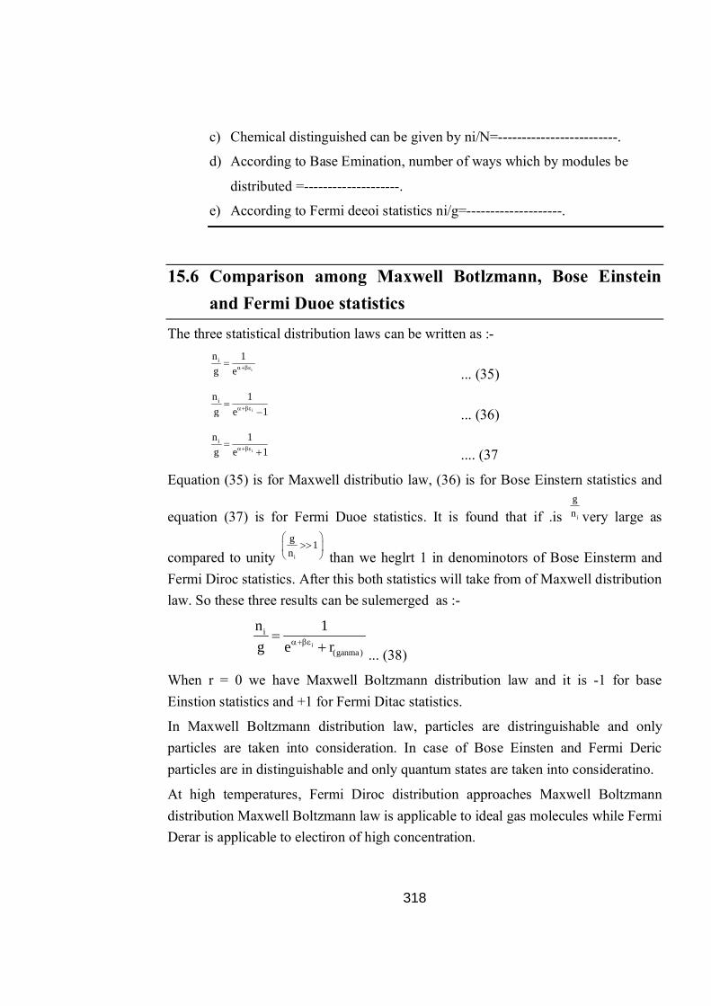
318

c) Chemical distinguished can be given by ni/N=-------------------------.

d) According to Base Emination, number of ways which by modules be

distributed =--------------------.

e) According to Fermi deeoi statistics ni/g=--------------------.

15.6 Comparison among Maxwell Botlzmann, Bose Einstein and Fermi Duoe statistics

The three statistical distribution laws can be written as :-

i

in 1g e

... (35)

i

in 1g e –1

... (36)

i

in 1g e 1

.... (37

Equation (35) is for Maxwell distributio law, (36) is for Bose Einstern statistics and

equation (37) is for Fermi Duoe statistics. It is found that if .is i

gn very large as

compared to unity i

g 1n

than we heglrt 1 in denominotors of Bose Einsterm and Fermi Diroc statistics. After this both statistics will take from of Maxwell distribution law. So these three results can be sulemerged as :-

i

i

(ganma)

n 1g e r

... (38)

When r = 0 we have Maxwell Boltzmann distribution law and it is -1 for base Einstion statistics and +1 for Fermi Ditac statistics.

In Maxwell Boltzmann distribution law, particles are distringuishable and only particles are taken into consideration. In case of Bose Einsten and Fermi Deric particles are in distinguishable and only quantum states are taken into consideratino.

At high temperatures, Fermi Diroc distribution approaches Maxwell Boltzmann distribution Maxwell Boltzmann law is applicable to ideal gas molecules while Fermi Derar is applicable to electiron of high concentration.

319

15.7 Summary

Boltzmann Maxwell distribution law is defined

Langranges method of undertermined multiplirs is used to solve maximum and minimum values for sufficient function. It relate independent variables with dependent variables.

Maxwell distribution law shows come limitations

In Bose Einster in statistics particles are considered to be indistinguished

Stirtlng formula is used to derive different statistics

Comparision between different statistics show that as high temperature, Fermi Dirac distribution approaches Maxwell Boltzmann distribution.

15.7 Glossary

Occupation number:-- number of systems in that particular state.

Thermodynamic probalility:- Number of microstaties Corresponding to that

microstatics.

Probalule distribution :-- Distribution of mopdular is a way that is maximum.

Distinguisable particles:-- two particles interchange their position or energy

states.


15.1 a) non- equilibirium b) extensure c) ground d) zero e) irreversible f) E W/JixI g)

Common

15.8 Review question a) Short Answer Type

1. Write equation to represent Boltzmann Maxwell distribution law.

2. Write stirling formoula for ln N.

3. What are various steps for using Long ranges method of uadetermined multipliers?

320

4. Give limitations of Maxwell Boltzmann statistics

5. Which type of particles are considered for Bose Einsteim and Fermi Diroc statistics?

6. How will you compare Maxwell Boltzmann, Bose Einsterm and Fermi Diror statistics?

b) Long Answer Type

1. Define Boltzmann Maxell distribution law using stirling formula and Langraphes ranges method of undetermined multipliers.

2. Define Bose Einster in statistics using method of uadetermined multipliers.

3. Describe Fermi Dirac statistics to determine maximum probability for distribution of particles.

4. How different statistics are intereleted with each other? What is the effect of temperature on Fermi Duar distribution.

5. Describe Lang ranges method of uadetermined multiplers. Write various steps envolue in it.

15.9 References and suggested readings 1. Advanced Physical Chmistry - Gurdeep Raj

2. Physical Cehestry - David W. Ball

3. Physical Cehestry - R.S. Rastogi

4. Advanced Physical Cehestry - J.N. Gurtu and A Gurtu

5. Physical Cehestry - Peter Atkins, Juliod Paula

6. Physical Cehestry - G.K. Vemulopalli

7. Principal of Physical Cehestry - Puri, Sharma, Pathania

321

Unit-16 : Non-equilibrium thermodynamics and Significance

Structure of Unit

16.0 Objective

16.1 Introduction

16.2 Non-equilibrium thermodynamics

16.3 Stationary states, fluctuations, and stability

16.4 Thermal Fluctuation

16.5 Phase transitions

16.6 Entropy production for irreversible process

16.7 Entropy production


16.9 Flux and Forces

16.10 Coupled Reactions

16.11 Summary

6.12 Glossary

Answer to Key anssesment Questions


16.14 References and Suggested readings

16.0 Objective

After a careful reading of this unit, you will be able to

Know what is nonequilibrium thermodynamics?

Understand the conditions of nonequilibrium thermodynamics.

Explain Stationary states, fluctuations, and stability.

Understand Thermal Fluctuation and phase transitions.

Know what is entropy production and irreversible processes.

322

Understand flux and forces and coupled reactions.

16.1 Introduction

This unit deals with non-equilibrium thermodynamics which describes transport processes in systems that are out of global equilibrium. The field resulted from the work of many scientists with the overriding aim to find a more useful formulation of the second law of thermodynamics in such systems. Onsager is counted as the founder of the field. Onsager was given the Nobel prize in chemistry in 1968 for these works. In non-equilibrium thermodynamics, the second law is redefined in terms of the local entropy production in the system, using the assumption of local equilibrium.

The non-equilibrium thermodynamics is important because, the most common industrial and living systems have transport of heat, mass and charge, alone or in combination with a chemical reaction. The process industry, the electrochemical industry, biological systems, as well as laboratory experiments, all concern heterogeneous systems, and are not in global equilibrium. There are four major reasons increases the importance of non-equilibrium thermodynamics is important for such systems. In the first place, the theory gives an accurate description of coupled transport processes. In the second plase, a framework is obtained for the definition of experiments. In the third plase; the theory quantifies not only the entropy that is produced during transport, but also the work that is done and the lost work. Last but not least, this theory allows us to check that the thermodynamic equations which we use to model our system, are in agreement with the second law. This unit also deals with conditions of nonequilibrium thermodynamics, Stationary states, fluctuations, and stability, Thermal Fluctuation and phase transitions, entropy production and irreversible processes, flux and forces and coupled reactions

16.2 Non-equilibrium thermodynamics

Non-equilibrium thermodynamics is a branch of thermodynamics that deals with the thermodynamic systems that are not in thermodynamic equilibrium. Most systems found in nature are not in thermodynamic equilibrium, as they are changing or can be triggered to change over time, and are continuously and discontinuously subject to flux of matter and energy to and from other systems and to chemical reactions. Non-

323

equilibrium thermodynamics is concerned with the rates of chemical reactions and with transport processes. Many natural systems still today remain beyond the scope of currently known macroscopic thermodynamic methods.

A system that is neither simply isolated from the rest of the universe, nor in contact with a constant temperature, and/or chemical potential path, will be nonequilibrium. A system that is in the transient before reaching equilibrium is also nonequilibrium, for example plasma with a non-Maxwellian velocity distribution scopertapary. An interesting nonequilibrium situation that will arise in later examples is a system in contact with two constant temperature paths that are at different temperatures. The nonequilibrium state may also be maintained by external fields, such as the electric field driving an electric current around a conducting loop. Features that may be associated with nonequilibrium are dynamics (for example the transient relaxation towards equilibrium), and currents of the conserved quantities from one part of the system to another. Indeed we have seen that the lifetime of the nonequilibrium state is likely to be very short unless there are macroscopic disturbances in the conserved quantities away from the equilibrium distribution. Accompanying these disturbances will be macroscopic currents of the conserved quantities.

The study of non-equilibrium systems with respect to the thermodynamics requires more general concepts than are dealt with by equilibrium thermodynamics. One fundamental difference between equilibrium thermodynamics and non-equilibrium thermodynamics lies in the behaviour of homogeneous systems, which require for their study knowledge of rates of reaction which are not considered in equilibrium thermodynamics of homogeneous systems. This is discussed below. Another fundamental difference is the difficulty in defining entropy in macroscopic terms for systems not in thermodynamic equilibrium.

There are many illustrations of stationary non-equilibrium systems, some very simple, like a system confined between two thermostates at different temperatures or a fluid enclosed between two flat walls moving in opposite directions and defining non-equilibrium conditions at the walls. Laser action is also a non-equilibrium process, but it depends on departure from local thermodynamic equilibrium and is thus beyond the scope of classical irreversible thermodynamics; here a strong temperature difference is maintained between two molecular degrees of freedom (with molecular laser, vibrational and rotational molecular motion), the requirement for two component 'temperatures' in the one small region of space, precluding local

324

thermodynamic equilibrium, which demands that only one temperature be needed. Damping of acoustic perturbations or shock waves are non-stationary non-equilibrium processes. Driven complex fluids, turbulent systems and glasses are other examples of non-equilibrium systems. Classes

The mechanics of macroscopic systems depends on a number of extensive quantities. It should be stressed that all systems are permanently interacting with their surroundings, thereby causing unavoidable fluctuations of extensive quantities. Equilibrium conditions of thermodynamic systems are related to the maximum property of the entropy. If the only extensive quantity that is allowed to fluctuate is the internal energy, all the other ones being kept strictly constant, the temperature of the system is measurable and meaningful. The system's properties are then most conveniently described using the thermodynamic potential Helmholtz free energy (A = U - TS), a Legendre transformation of the energy. If, next to fluctuations of the energy, the macroscopic dimensions (volume) of the system are left fluctuating, we use the Gibbs free energy (G = U + PV - TS), where the system's properties are determined both by the temperature and by the pressure.

An interesting nonequilibrium situation is one in which there is no time dependence (i.e. a steady state situation), but one in which currents of the conserved variables are flowing, driven by injection at one boundary and subtraction at another. Since the dynamics of the system are dissipative, there will usually be an injection of energy, energy currents within the system, sometimes a transformation between different forms of energy (e.g. mechanical or chemical to heat), and then the subtraction of energy to maintain the steady state. For example the system in contact with two heat baths at different, but constant, temperatures, will exhibit energy currents transporting heat between the two baths.

Non-equilibrium systems are much more complex and they may undergo fluctuations of more extensive quantities. The boundary conditions impose on them particular intensive variables, like temperature gradients or distorted collective motions often called thermodynamic forces. If free energies are very useful in equilibrium thermodynamics, it must be stressed that there is no general law defining stationary non-equilibrium properties of the energy as is the second law of thermodynamics for the entropy in equilibrium thermodynamics.

325

16.3 Stationary states, fluctuations, and stability

In thermodynamics a stationary state of a process is often interesting, allowing that the stationary state include the occurrence of unpredictable and experimentally unreproducible fluctuations in the state of the system. The fluctuations are due to the system's internal sub-processes and to exchange of matter or energy with the system's surroundings that create the constraints that define the process.

If the stationary state of the process is stable, then the unreproducible fluctuations involve local transient decreases of entropy. The reproducible response of the system is then to increase the entropy back to its maximum by irreversible processes: the fluctuation cannot be reproduced with a significant level of probability. Fluctuations about stable stationary states are extremely small except near critical points. The stable stationary state has a local maximum of entropy and is locally the most reproducible state of the system. There are theorems about the irreversible dissipation of fluctuations. Here 'local' means local with respect to the abstract space of thermodynamic coordinates of state of the system.

If the stationary state is unstable, then any fluctuation will almost surely trigger the virtually explosive departure of the system from the unstable stationary state. This can be accompanied by increased export of entropy.

16.4 Thermal Fluctuation

The familiar macroscopic equations of fluid dynamics, thermal and particle diffusion etc. can be thought of as averages over the underlying microscopic molecular dynamics. At macroscopic length scales the root mean square fluctuations about the mean values are much smaller than the mean values by factors of order N−1 = 2 where N is the number of molecular degrees of freedom in the averaging volume. This is because the fluctuations tend to cancel in the summation to form the macroscopic variable saperatopara. For the length scales of order mm;cm, or larger of most pattern forming systems the size of the fluctuating corrections to the macroscopic deterministic equations are very small indeed. The constraint that the fluctuating forces must yield a distribution of the thermodynamics variables given by the Boltzmann factor (i.e. probability proportional to (exp−bE) with b = 1/kBT with kB the Boltzmann constant and E the energy, or more precisely the free energy, of the fluctuation), and the observation that the stochastic effects due to individual molecular collisions act on time scales very short compared to the macroscopic

326

phenomenon of interest, are sufficient to pin down the strength and character of the fluctuating forces. Aprofound result of statistical mechanics known as the fluctuation-dissipation theorem in fact directly relates the strength of the fluctuating forces to the dissipative kinetic coefficients in the macroscopic equations, and to the temperature.

16.5 Phase transitions

The phase transitions is important in equilibrium physics, and analogous phenomena play an equally important role in the formation of structures in nonequilibrium systems. Phase transitions are also important to our discussion because they lead to states that require additional thermodynamic variables for a complete characterization, requiring us to expand our list of thermodynamic variables introduced above, through the idea of broken symmetries seperatapara. Consider a simple thermodynamic system made up of a large number N of spins si that are arranged on a simple lattice (e.g. a cubic lattice in 3 dimensional space). Suppose that each spin si can only point in two directions, “up” Si = 1 or “down” Si = −1. (This would be the case for spin 1/2 quantum spins where the up-down direction is an arbitrary choice of the quantization directions, or for other spins in a system with anisotropy energies such as crystal field energies that favor two degenerate opposite orientations with respect to others.) Now suppose that there is an energy of interaction between nearest neighbor spins that is lower if the spins are parallel.

This means the total energy can be written:

…………(6.1)

At high temperatures kBT >> J where thermal fluctuations kBT are much larger than this interaction energy, the interaction will be unimportant, and the individual spins

will fluctuate randomly up or down. The total macroscopic spin, S = < > summed over all lattice sites and averaged over thermal fluctuations, will be zero.

On the other hand at low temperatures the interaction favors parallel alignment of spins. At lower temperatures the interaction will dominate, and the system will tend to its ground state. However we see that there are two possible degenerate ground states in which all the spins are parallel: all spins up or all spins down. The total spin S is either N or −N. In principle, since the two configurations are degenerate, we

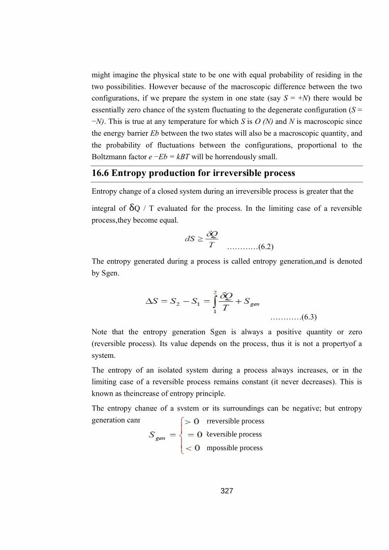
327

might imagine the physical state to be one with equal probability of residing in the two possibilities. However because of the macroscopic difference between the two configurations, if we prepare the system in one state (say S = +N) there would be essentially zero chance of the system fluctuating to the degenerate configuration (S = −N). This is true at any temperature for which S is O (N) and N is macroscopic since the energy barrier Eb between the two states will also be a macroscopic quantity, and the probability of fluctuations between the configurations, proportional to the Boltzmann factor e −Eb = kBT will be horrendously small.

16.6 Entropy production for irreversible process

Entropy change of a closed system during an irreversible process is greater that the

integral of δQ / T evaluated for the process. In the limiting case of a reversible process,they become equal.

…………(6.2)

The entropy generated during a process is called entropy generation,and is denoted by Sgen.

…………(6.3)

Note that the entropy generation Sgen is always a positive quantity or zero (reversible process). Its value depends on the process, thus it is not a propertyof a system.

The entropy of an isolated system during a process always increases, or in the limiting case of a reversible process remains constant (it never decreases). This is known as theincrease of entropy principle.

The entropy change of a system or its surroundings can be negative; but entropy generation cannot.

Irreversible process

Reversible process

Impossible process

328

………(6.)

three conditions can be explained as

A process must proceeds in the direction that complies with the increase of entropy principle, Sgen > 0.

Entropy is a non‐conserved property, and there is no such thing as the conservation of entropy. Therefore, the entropy of universe is continuously increasing.

The performance of engineering systems is degraded by the presence of irreversibility. The entropy generation is a measure of the magnitudes of the irreversibilities present during the process.

16.7 Entropy production

It determines the performance of thermal machines such as power plants, heat engines, refrigerators, heat pumps, and air conditioners. It also plays a key role in the thermodynamics of irreversible processes. Entropy is produced in irreversible processes. The importance of avoiding irreversible processes (hence reducing the entropy production) was recognized as early as 1824 by Carnot. In 1867 Rudolf Clausius expanded his previous work from 1854 on the concept of “unkompensierte Verwandlungen” (uncompensated transformations), which, in our modern nomenclature, would be called the entropy production. In the same article as where he introduced the name entropy, Clausius gives the expression for the entropy production (for a closed system), which he denotes by N.

…………(6.5)

Here S is entropy in the final state and the integral is to be taken from the initial state to the final state. From the context it is clear that N = 0 if the process is reversible and N > 0 in case of an irreversible process.

The laws of thermodynamics apply to well-defined systems. We consider systems which, in general, are inhomogeneous. Heat and mass are transferred across the boundaries (non adiabatic, open systems), and the boundaries are moving (usually through pistons). In our formulation we assume that heat and mass transfer and volume changes take place only at well-defined regions of the system boundary. The

329

expression, given here, are not the most general formulations of the first and second law. E.g. kinetic energy and potential energy terms are missing and exchange of matter by diffusion is excluded.

In the stationary state, irreversible systems are in a continuous process of production of entropy. A measure of the distance from thermodynamic equilibrium can therefore be given by the production of entropy since this quantity vanishes in equilibrium. The rate of change of the entropy S of a system can be properly decomposed into two contributions

dS / dt = F – P …………(6.6)

Where P is the entropy production due to irreversible processes which ocurring inside the system and F is the entropy flux from the system to the environment. The quantity P is positive definite whereas F can have either sign. In the stationary state the rate of change of the entropy vanishes so that F = P. The quantity F is defined as the flux from inside to outside the system, so that it will be positive in the nonequilibrium stationary state.

In equilibrium the entropy is a well defined quantity, in non equilibrium systems the entropy as well as the production of entropy do not have a universal definition. According to Gallavotti the problem of defining entropy in a system out of equilibrium has not been solved yet. In this sense it is interesting to see how one can define those quantities in systems that evolve in time according to specified dynamics. In deterministic Hamiltonian dynamics it is well known that the Gibbs entropy is invariant. This property is a consequence of the incompressibility of the “fluid” that represents the system in phase space. Irreversible systems, on the other hand, are supposed to be described by non Hamiltonian dynamics, that is, by dynamics coming from nonconservative forces. In this case, the “fluid” in phase space becomes compressible and the production of entropy may be related to the contraction of the phase space


A process that is not reversible is called irreversible. This concept arises most frequently in thermodynamics, as applied to processes.

In thermodynamics, a change in the thermodynamic state of a system and all of its surroundings cannot be precisely restored to its initial state by infinitesimal changes

330

in some property of the system without expenditure of energy. A system that undergoes an irreversible process may still be capable of returning to its initial state; however, the impossibility occurs in restoring the environment to its own initial conditions. An irreversible process increases the entropy of the universe. However, because entropy is a state function, the change in entropy of a system is the same whether the process is reversible or irreversible. The second law of thermodynamics can be used to determine whether a process is reversible or not.

All complex natural processes are irreversible. The phenomenon of irreversibility results from the fact that if a thermodynamic system, which is any system of sufficient complexity, of interacting molecules is brought from one thermodynamic state to another, the configuration or arrangement of the atoms and molecules in the system will change in a way that is not easily predictable. A certain amount of "transformation energy" will be used as the molecules of the "working body" do work on each other when they change from one state to another. During this transformation, there will be a certain amount of heat energy loss or dissipation due to intermolecular friction and collisions; energy that will not be recoverable if the process is reversed.

Many biological processes that were once thought to be reversible have been found to actually be a pairing of two irreversible processes. Whereas a single enzyme was once believed to catalyze both the forward and reverse chemical changes, research has found that two separate enzymes of similar structure are typically needed to perform what results in a pair of thermodynamically irreversible processes.

Examples of irreversible processes

Entropy is produced in irreversible processes. Some important irreversible processes are:

heat flow through a thermal resistance

fluid flow through a flow resistance such as in the Joule expansion or the Joule-Thomson effect

diffusion

Joule heating

friction between solid surfaces.

331

The expression for the rate of entropy production in the first two cases will be derived in separate sections

chemical reactions

16.9 Flux and Forces

The simplest descriptions of heat, mass and charge transports are the equations of Fourier, Fick and Ohm. Fourier’s law expresses the measurable heat flux in terms of the temperature gradient by:

…………(6.7)

whereλ is the thermal conductivity, T is the absolute temperature, and the direction of transport is along the x-axis. Fick’s law gives the flux of one of the components in terms of the gradient of its concentration c:

…………(6.8)

where D is the diffusion coefficient. Similarly, Ohm’s law gives the electric current in terms of the gradient of the electric potential:

…………(6.9)

whereκ is the electrical conductivity, and φ is the electric potential. In a stationary state, there is no accumulation of internal energy, mass or charge. This means that the heat, molar and electric fluxes are independent of position. The derivatives of the above equations with respect to x are then zero:

…………(6.12)

332

These equations can be used to calculate the temperature, concentration and electric potential as a function of the position, when their values on the boundaries of the

system and λ, D and κ are known. Such a calculation is illustrated by the following exercise.

Flux-Force relationship

The non-equilibrium thermodynamics has as basis the entropy production, which has the general form:

…………(6.13)

where Ji and Xi are the so-called conjugate thermodynamic fluxes and forces. There are n independent flux-force pairs. The meaning of being conjugate shall be further discussed in the next section. A basic assumption in non-equilibrium thermodynamics is that each flux is a linear function of all forces:

………………(6.14)

The relationship is linear in the sense that the Onsager conductivity matrix Lij does not depend on Xj . The coefficients are functions of the state variables, for instance, like the local pressure and temperature, but not of the forces. The theory therefore prescribes that coefficients, like the thermal conductivity, can depend on the temperature, but not on the gradient of the temperature.

16.10 Coupled Reactions

A coupled reaction in biology is a chemical reaction having a common intermediate and in which energy is transferred from one side of the reaction to the other side. An example would be a molecule of sucrose being synthesised from glucose and fructose at the expense of the energy stored in ATP and transferred by glucose-1-phosphate.

Two or more reactions in a cell sometimes can be coupled so that thermodynamically unfavorable reactions and favorable reactions are combined to drive the overall process in the favorable direction. In this circumstance the overall free energy is the sum of individual free energies of each reaction. This process of coupling reactions is

333

carried out at all levels within cells. The predominant form of coupling is the use of compounds with high energy to drive unfavorable reactions.

The predominant form of high energy compounds in the cell are those which contain phosphate. Hydrolysis of the phosphate group can yield free energies in the range of –10 to –62 kJ/mol. These molecules contain energy in the phosphate bonds due to:

1. Resonance stabilization of the phosphate products

2. Increased hydration of the products

3. Electrostatic repulsion of the products

4. Resonance stabilization of products

5. Proton release in buffered solutions

Examples of Coupled Reactions in Biology

Consider the hypothetical reaction: A ——> B. If this is a thermodynamically

unfavorable reaction the ΔG' value will be positive. Let's assume it is +4.0 kcal/mol. In order to drive this reaction in the direction written it can be coupled to the hydrolysis of ATP. The free energy of ATP hydrolysis to ADP is shown:

ATP + H2O ——> ADP + Pi ΔG = –7.3 kcal/mol

Coupling the two reactions together gives the equation:

A + ATP + H2O ——> B + ADP + Pi + H+

The ΔG for this coupled reaction is the sum of the ΔG values of the two separate reactions, i.e. (-7.3kcal/mol) + (+4.0kcal/mol) = -3.3kcal/mol. This indicates that coupling ATP hydrolysis provides the energy necessary to make the conversion of A to B thermodynamically favorable.

Another useful example is to examine one of the reactions of glycolysis. In this case we will look at the oxidation of phosphoenolpyruvate to pyruvate catalyzed by the enzyme pyruvate kinase (PK).

phosphoenolpyruvate ——> pyruvate ΔG = –14.7 kcal/mol

This reaction releases sufficient energy to drive the synthesis of ATP from ADP and

Pi which would normally be thermodynamically unfavorable with a ΔG of +7.3kcal/mol. Note that this value is the reciprocal of the hydrolysis of ATP. This

points out another fact that the ΔG for a reaction in one direction is equal but

334

mathematically opposite for the reciprocal direction. Coupling the two reactions together yields:

phosphoenolpyruvate + ADP + H+ ——> pyruvate + ATP ΔG = –7.4 kcal/mol

Fill in the blanks (After 16.10) a) A systems in the transient before reaching equilibrium is -----------------. b) Macroscope system depends on number of ---------------quantities. c) At lower temperature, the systems lend to it ---------state . d) for reversible process Sgen=--------------------. e) the process that is not reversible is ---------------. f) flux force relationship is given us---------------. g) A coupled relation has ----------------intermediates.

16.11 Summary

Non-equilibrium thermodynamics is a branch of thermodynamics that deals with the thermodynamic systems that are not in thermodynamic equilibrium. Non-equilibrium thermodynamics is concerned with the rates of chemical reactions and with transport processes. Many natural systems still today remain beyond the scope of currently known macroscopic thermodynamic methods.

The fluctuations are due to the system's internal sub-processes and to exchange of matter or energy with the system's surroundings that create the constraints that define the process.

A profound result of statistical mechanics known as the fluctuation-dissipation theorem in fact directly relates the strength of the fluctuating forces to the dissipative kinetic coefficients in the macroscopic equations, and to the temperature.

The phase transitions is important in equilibrium physics, and analogous phenomena play an equally important role in the formation of structures in nonequilibrium systems.

335

The entropy change of a system or its surroundings can be negative; but entropy

generation cannot.

There are deffierent three conditions can be explained as

A process must proceeds in the direction that complies with the increase of entropy principle, Sgen > 0.

Entropy is a non‐conserved property, and there is no such thing as the conservation of entropy. Therefore, the entropy of universe is continuously increasing.

A process that is not reversible is called irreversible. This concept arises most frequently in thermodynamics, as applied to processes.

A system that undergoes an irreversible process may still be capable of returning to its initial state; however, the impossibility occurs in restoring the environment to its own initial conditions. An irreversible process increases the entropy of the universe. However, because entropy is a state function, the change in entropy of a system is the same whether the process is reversible or irreversible. The second law of thermodynamics can be used to determine whether a process is reversible or not.

16.12 Glossary

Non equrilibrium :-- system away from equilibirium.

Entropy:-- Randomnes in the systems.

Flux:-- The gradient due to which form of energy, matter takes place.

Sattionary states:-- Microscopic properties do not change with time.

Biological systems:-- Living phenomenon systems


16.1 a) π—n b) longer c) Hypsochomie d) longer

336


1. What is non equilibrium thermodynamics? Explain 2. Explain entropy production in irreversible process. 3. Explain flux and forces. 4. Describe coupled reaction with examples. 5. What is phase transition? 6. What is thermal flucatuation? 7. Explain stationary phases. 8. What is stability.

16.14 References and Suggested readings

1. Non-Equilibrium Thermodynamics of Heterogeneous Systems Signe Kjelstrup Dick Bedeaux world scientific publishing co. ltd ( 2008).

2. http://en.wikipedia.org/wiki/Non-equilibrium_thermodynamics. 3. Physical Chemistry- Robert G. Mortimer (3rdEd), Elsevier Academic Press (2008)

337

Unit – 17 : UV-visible spectroscopy Structure of Unit:

17.0 Objectives

17.1 Introduction

17.2 The Chromophore Concept

17.3 Auxochromes

17.4 Absorption and Intensity Shift

17.5 Origin of UV-visible spectra

17.6 Types of Electronic Transitions

17.7 Principle of UV-Visible absorption

17.8 Instrumentation

17.9 Solvents

17.10 Applications of UV-Vis spectroscopy

17.11 Summary

17.12 Glossary

Answer to Key anssesment Questions

17.13 Multiple Choice Questions



338

At the end of the unit learner will be able to understand make a bullat the principle and various applications of UV-Visible spectroscopy absorption of light by solution is one of the oldest and still one of the more useful instrumental methods. The wavelength of light that a compound will absorb is characteristic of its chemical structure. Absorption of visible and ultraviolet (UV) radiation is associated with excitation of electrons, in both atoms and molecules, to higher energy states. All molecules will undergo electronic excitation following absorption of light, but for most molecules very high energy radiation (in the vacuum ultraviolet, <200 nm) is required. The wavelength associated with the molecules can be calculated by using Woodward-Fieser rule. It is very useful to measure the number of conjugated double bonds and also aromatic conjugation in various molecules.

17.1 Introduction

Ultraviolet (UV) and visible radiation comprise only a small part of the electromagnetic spectrum, which includes such other forms of radiation as radio, infrared (IR), cosmic, and X rays (Figure 17.1). The energy associated with electromagnetic radiation is defined by the following equation:

E = hν

Figure 17.1: The Electromagnetic Spectrum.

Where E is energy (in joules), h is Planck’s constant (6.62 × 10-34 Js), and ν is frequency (in seconds).

17.0 Objectives

339

Electromagnetic radiation can be considered a combination of alternating electric and magnetic fields that travel through space with a wave motion. Because radiation acts as a wave, it can be classified in terms of either wave length or frequency, which is related by the following equation: (17.2)

ν = c/λ ………………..(17.2)

whereν is frequency (in seconds), c is the speed of light(3 × 108 ms-1), and λ is wavelength (in meters). In UV-visible spectroscopy, wavelength usually is expressed in nanometers (1 nm = 10-9 m).It follows from the above equations that radiation with shorter wavelength has higher energy. In UV-visible spectroscopy, the low-wavelength UV light has the highest energy.

Ultraviolet–visible spectroscopy refers to absorption spectroscopy or reflectance spectroscopy in the ultraviolet-visible spectral region. This means it uses light in the visible and adjacent (near-UV and near-infrared (NIR)) ranges. The absorption or reflectance in the visible range directly affects the perceived color of the chemicals involved. In this region of the electromagnetic spectrum, molecules undergo electronic transitions. The alternate title for this spectroscopy is electronic spectroscopy since it involves the promotion of electrons from the ground state to higher energy state. This technique is useful in measuring aliphatic and aromatic conjugation in various molecules. It also distinguishes between conjugated and non-conjugated systems such as homoannular and heteroannular conjugated dienes.

17.2 The Chromophore Concept

Defination ; Chromophores are parts of a molecule that have electronic bands with energy differences comparable to the energies of the UV-visible light which is then absorbed by them. Chromophores, for example, dienes, nitriles, carbonyl, or carboxyl

groups often contain π bonds. Other types of chromophores are transition metal complexes and their ions. Molecules without chromophores, such as water, alkanes or alcohols, should be ideal solvents for UV-visible spectroscopy because they hardly show any absorbance themselves.

In the conjugated chromophores, the electrons jump between energy levels that are extended pi orbitals, created by a series of alternating single and double bonds, often in aromatic systems. Various factors in a chromophore's structure go into

340

determining at what wavelength region in a spectrum the chromophore will absorb. Lengthening or extending a conjugated system with more

unsaturated (multiple) bonds in a molecule will tend to shift absorption to longer wavelengths. Woodward-Fieser rules can be used to approximate ultraviolet-visible maximum absorption wavelength in organic compounds with conjugated pi-bond systems.

There are two types of chromophores:

(a) Chromophores in which the group contains π electrons and they undergo

ππ*transition. For examples ethylenes and acetylenes etc.

(b) Chromophores which contain both π electron and n electrons. Such

chromophores undergo two types of transitions i.e. ππ* and n π*. Examples of this type are carbonyls, nitriles, azo compounds, nitro compounds etc.

Isolated Double bond

Due to π→π* electronic transition unconjugated alkenes absorb below 200 nm, e.g.,

ethene shows an absorption at 171 nm. Alkyl substituents or the ring residues attached to the olefinic carbon shift the absorption band towards longer wavelength as can be seen with absorption pattern of compounds like 1-Octene and cyclohexene which absorb at 177 nm and 182 nm, respectively.

Conjugated dienes

With the increase in conjugation the absorption moves towards longer wavelengths, thus compared with ethene, which absorbs at 171nm, 1,3-butadiene absorbs at 217 nm. Sufficient conjugation shifts the absorption to wavelengths that reach the visible region of the spectrum.

341

Table 17.1: Electronic absorption of some common chromophores

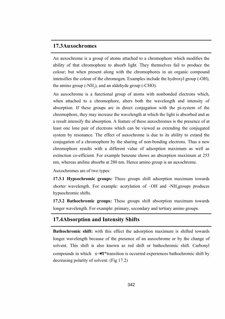
342

17.3Auxochromes

An auxochrome is a group of atoms attached to a chromophore which modifies the ability of that chromophore to absorb light. They themselves fail to produce the colour; but when present along with the chromophores in an organic compound intensifies the colour of the chromogen. Examples include the hydroxyl group (-OH), the amino group (-NH2), and an aldehyde group (-CHO).

An auxochrome is a functional group of atoms with nonbonded electrons which, when attached to a chromophore, alters both the wavelength and intensity of absorption. If these groups are in direct conjugation with the pi-system of the chromophore, they may increase the wavelength at which the light is absorbed and as a result intensify the absorption. A feature of these auxochromes is the presence of at least one lone pair of electrons which can be viewed as extending the conjugated system by resonance. The effect of auxochrome is due to its ability to extand the conjugation of a chromophore by the sharing of non-bonding electrons. Thus a new chromophore results with a different value of adsorption maximum as well as extinction co-efficient. For example benzene shows an absorption maximum at 255 nm, whereas aniline absorbs at 280 nm. Hence amino group is an auxochrome.

Auxochromes are of two types:

17.3.1 Hypsochromic groups: These groups shift adsorption maximum towards shorter wavelength. For example: acetylation of –OH and -NH2groups produces hypsochromic shifts.

17.3.2 Bathochromic groups: These groups shift absorption maximum towards longer wavelength. For example: primary, secondary and tertiary amino groups.

17.4Absorption and Intensity Shifts

Bathochromic shift: with this effect the adsorption maximum is shifted towards longer wavelength because of the presence of an auxochrome or by the change of solvent. This shift is also known as red shift or bathochromic shift. Carbonyl

compounds in which n π*transition is occurred experiences bathochromic shift by decreasing polarity of solvent. (Fig 17.2)

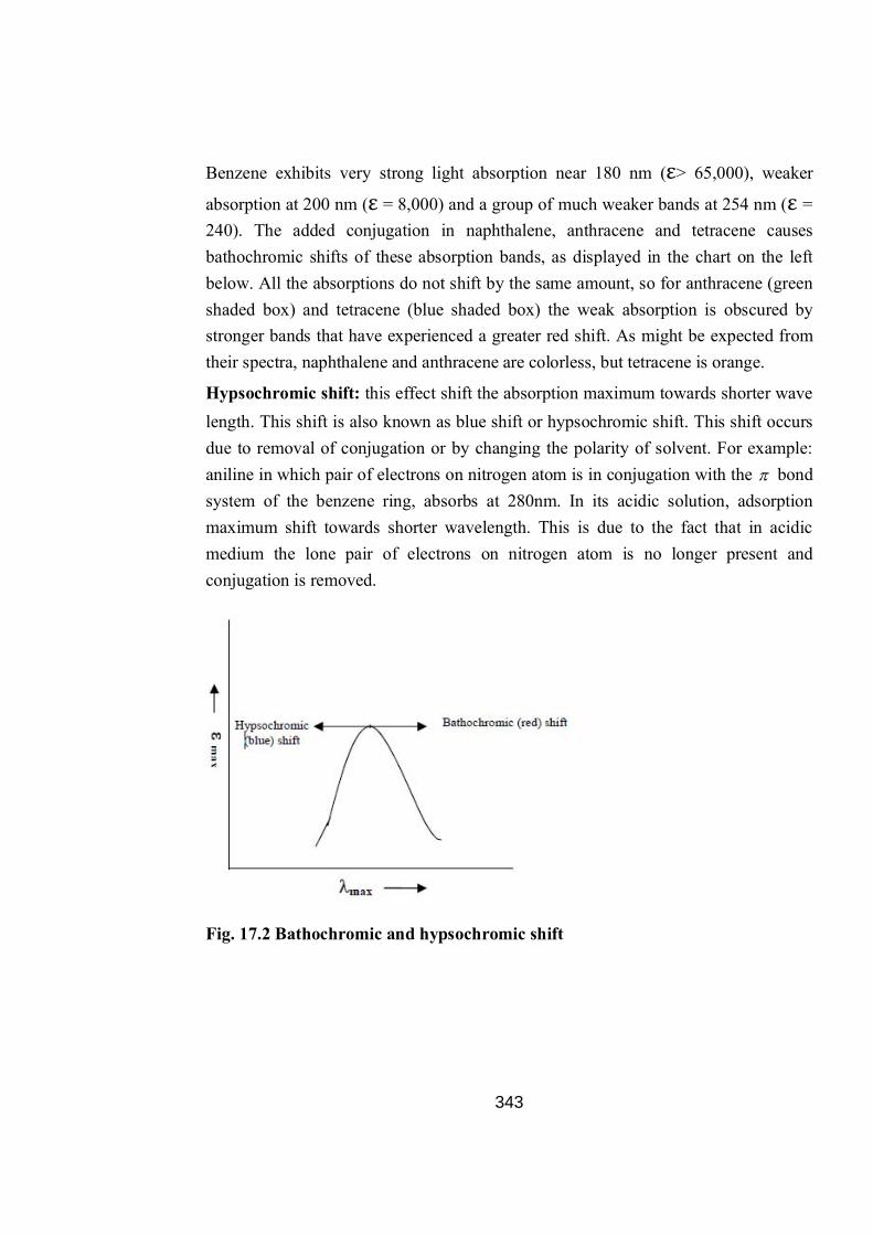
343

Benzene exhibits very strong light absorption near 180 nm (ε> 65,000), weaker

absorption at 200 nm (ε = 8,000) and a group of much weaker bands at 254 nm (ε = 240). The added conjugation in naphthalene, anthracene and tetracene causes bathochromic shifts of these absorption bands, as displayed in the chart on the left below. All the absorptions do not shift by the same amount, so for anthracene (green shaded box) and tetracene (blue shaded box) the weak absorption is obscured by stronger bands that have experienced a greater red shift. As might be expected from their spectra, naphthalene and anthracene are colorless, but tetracene is orange.

Hypsochromic shift: this effect shift the absorption maximum towards shorter wave length. This shift is also known as blue shift or hypsochromic shift. This shift occurs due to removal of conjugation or by changing the polarity of solvent. For example: aniline in which pair of electrons on nitrogen atom is in conjugation with the bond system of the benzene ring, absorbs at 280nm. In its acidic solution, adsorption maximum shift towards shorter wavelength. This is due to the fact that in acidic medium the lone pair of electrons on nitrogen atom is no longer present and conjugation is removed.

Fig. 17.2 Bathochromic and hypsochromic shift

344

17.5 Origin of UV-visible spectra

When radiation interacts with matter, a number ofprocesses can occur, including reflection, scattering,absorbance, fluorescence/phosphorescence (absorptionand reemission), and photochemical reaction (absorbanceand bond breaking). In general, when measuring UV-visible spectra, we want only absorbance to occur.Because light is a form of energy, absorption of light bymatter causes the energy content of the molecules (oratoms) to increase. The total potential energy of a moleculegenerally is represented as the sum of its electronic,vibrational, and rotational energies:

Etotal=Eelectronic +Evibrational + Erotational

The amount of energy a molecule possesses in each form is sepenate the term not a continuum but a series of discrete levels or states. Thedifferences in energy among the different states are in theorder:

Eelectronic>Evibrational>Erotational

Figure 17.3 : Electronic transition in formaldehyde

In some molecules and atoms, photons of UV and visible light have enough energy to cause transitions between the different electronic energy levels. The wavelength of light absorbed is that having the energy required to move an electron from a lower energy level to a higher energy level. Figure 17.3 shows an example of electronic transitions in formaldehyde and the wavelengths of light that cause them.These transitions should result in very narrow absorbance bands at wavelengths highly characteristic of the difference in energy levels of the absorbing species. This is true for atoms, as depicted in Figure 17.4.

345

Figure 17.4: Electronic transition in atoms.

However, for molecules, vibrational and rotational energy levels are superimposed on the electronic energy levels. Because many transitions with different energies can occur, the bands are broadened (Figure 17.5). The broadening is even greater in solutions owing to solvent-solute interactions.

Figure 17.5: Electronic transitions in molecules.

17.6 Types of Electronic Transitions

The absorption of UV or visible radiation corresponds to the three types of electronic transition:

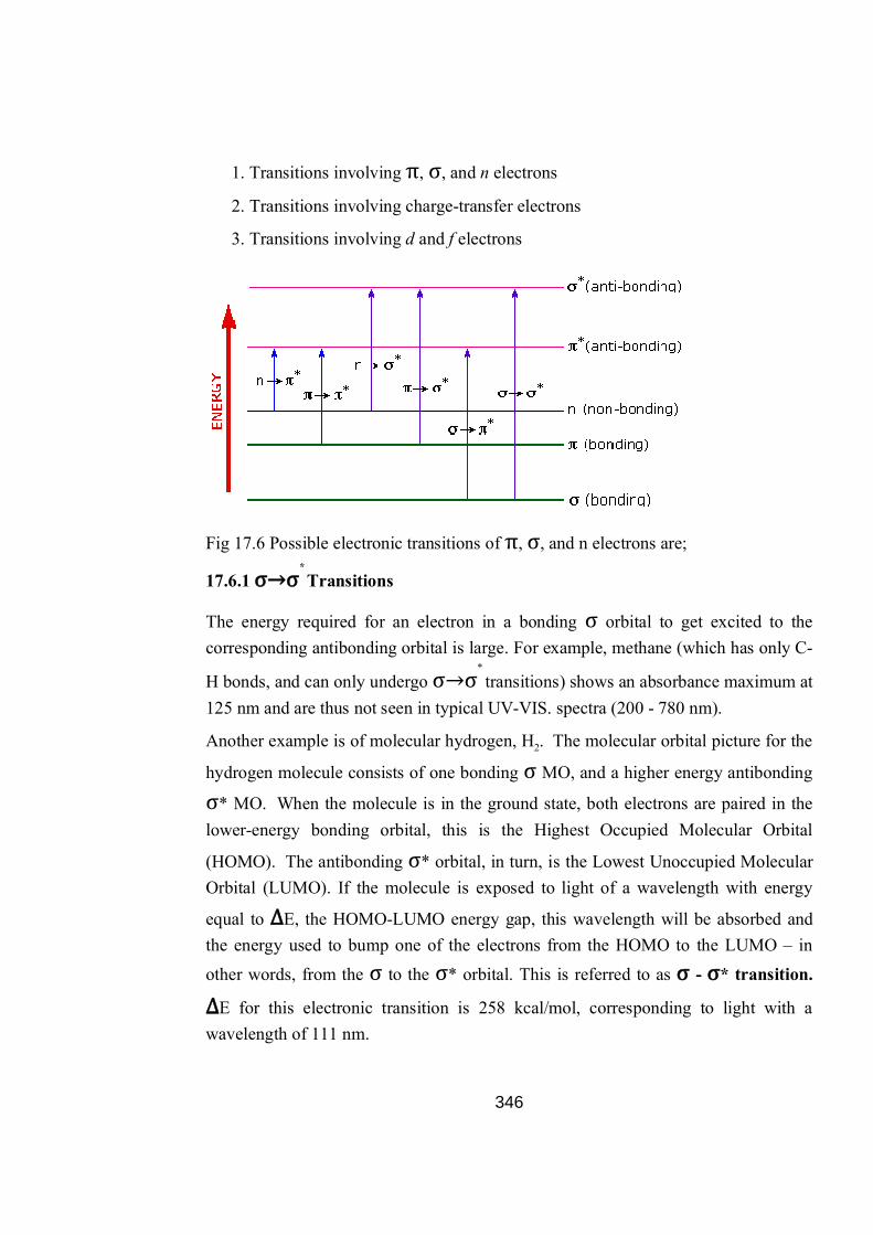
346

1. Transitions involving π, σ, and n electrons

2. Transitions involving charge-transfer electrons

3. Transitions involving d and f electrons

Fig 17.6 Possible electronic transitions of π, σ, and n electrons are;

17.6.1 σ→σ* Transitions

The energy required for an electron in a bonding σ orbital to get excited to the corresponding antibonding orbital is large. For example, methane (which has only C-

H bonds, and can only undergo σ→σ* transitions) shows an absorbance maximum at

125 nm and are thus not seen in typical UV-VIS. spectra (200 - 780 nm).

Another example is of molecular hydrogen, H2. The molecular orbital picture for the

hydrogen molecule consists of one bonding σ MO, and a higher energy antibonding

σ* MO. When the molecule is in the ground state, both electrons are paired in the lower-energy bonding orbital, this is the Highest Occupied Molecular Orbital

(HOMO). The antibonding σ* orbital, in turn, is the Lowest Unoccupied Molecular Orbital (LUMO). If the molecule is exposed to light of a wavelength with energy

equal to ΔE, the HOMO-LUMO energy gap, this wavelength will be absorbed and the energy used to bump one of the electrons from the HOMO to the LUMO – in other words, from the σ to the σ* orbital. This is referred to as σ - σ* transition.

ΔE for this electronic transition is 258 kcal/mol, corresponding to light with a wavelength of 111 nm.

347

Fig 17.7 Homo and LUMO states

17.6.2 n→σ* Transitions

Saturated compounds containing atoms with lone pairs (non-bonding electrons) like

saturated alcohols, amines, halides, ethers etc are capable of showing n →σ*

transitions. Energy required for these transitions is usually less than σ→σ*

transitions. Such compounds absorb light having wavelength in the range 150 - 250 nm, e.g., absorption maxima for water, methyl chloride and methyl iodide are 167 nm, 169 nm and 258 nm respectively.

17.6.3 π→π* Transitions

These transitions need an unsaturated group in the molecule to provide the π electrons. , eg., in alkenes, alkynes, aromatics, acyl compounds or nitriles. Most

absorption spectroscopy of organic compounds is based on transitions of n or π

electrons to the π* excited state and the absorption peaks for these transitions fall in

an experimentally convenient region of the spectrum (200 - 780 nm). π→π*

transitions normally give molar absorptivities between 1000 and 10,000 L mol-1

cm-

10. Unconjugated alkenes absorb at 170-190 nm. For example in case of ethene

molecule, ethene absorbs light at 165 nm, a longer wavelength than molecular hydrogen.

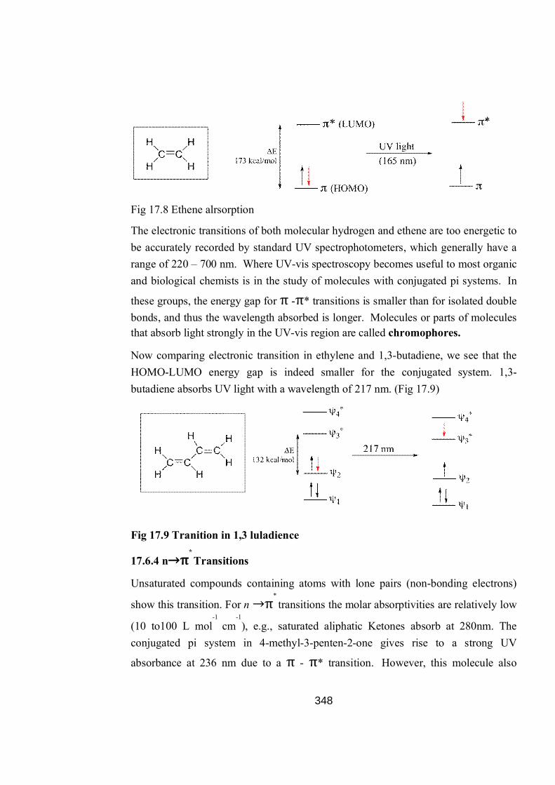
348

Fig 17.8 Ethene alrsorption

The electronic transitions of both molecular hydrogen and ethene are too energetic to be accurately recorded by standard UV spectrophotometers, which generally have a range of 220 – 700 nm. Where UV-vis spectroscopy becomes useful to most organic and biological chemists is in the study of molecules with conjugated pi systems. In

these groups, the energy gap for π -π* transitions is smaller than for isolated double bonds, and thus the wavelength absorbed is longer. Molecules or parts of molecules that absorb light strongly in the UV-vis region are called chromophores.

Now comparing electronic transition in ethylene and 1,3-butadiene, we see that the HOMO-LUMO energy gap is indeed smaller for the conjugated system. 1,3-butadiene absorbs UV light with a wavelength of 217 nm. (Fig 17.9)

Fig 17.9 Tranition in 1,3 luladience

17.6.4 n→π* Transitions

Unsaturated compounds containing atoms with lone pairs (non-bonding electrons)

show this transition. For n →π* transitions the molar absorptivities are relatively low

(10 to100 L mol-1

cm-1), e.g., saturated aliphatic Ketones absorb at 280nm. The

conjugated pi system in 4-methyl-3-penten-2-one gives rise to a strong UV

absorbance at 236 nm due to a π - π* transition. However, this molecule also

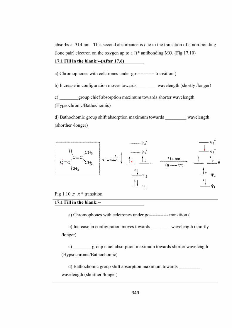
349

absorbs at 314 nm. This second absorbance is due to the transition of a non-bonding

(lone pair) electron on the oxygen up to a π* antibonding MO. (Fig 17.10)

17.1 Fill in the blank:--(After 17.6)

a) Chromophones with eelctrones under go------------ transition (

b) Increase in configuration moves towards ________ wavelength (shortly /longer)

c) ________group chief absorption maximum towards shorter wavelength

(Hypsochronic/Bathochomic)

d) Bathochomic group shift absorption maximum towards _________ wavelength

(shorther /longer)

Fig 1.10 * transition

17.1 Fill in the blank:--

a) Chromophones with eelctrones under go------------ transition (

b) Increase in configuration moves towards ________ wavelength (shortly

/longer)

c) ________group chief absorption maximum towards shorter wavelength

(Hypsochronic/Bathochomic)

d) Bathochomic group shift absorption maximum towards _________

wavelength (shorther /longer)

350

17.7 Principle of UV-Visible absorption

Molecules containing π-electrons or non-bonding electrons (n-electrons) can absorb the energy in the form of ultraviolet or visible light to excite these electrons to higher anti-bonding molecular orbitals. The more easily excited the electrons (i.e. lower energy gap between the HOMO and the LUMO), the longer the wavelength of light it can absorb.

17.7.1 The Adsorption Laws (Beer-Lambert law):

The Beer-Lambert law (or Beer's law) is the linear relationship between absorbance and concentration of an absorbing species. The general Beer-Lambert law is usually written as:

…..(17.3)

Where A is the measured absorbance, l is the path length, and c is the analyte concentration. When working in concentration units of molarity, isthe molar absorptivity coefficient with units of M-1 cm-1.

Experimental measurements are usually made in terms of transmittance (T), which is defined as: T =I/Io ……..(17.4) where I is the light intensity after it passes through the sample and Io is the initial light intensity. The relation between A and T is:

A = -log T = - log (I / Io) …..(17.5)

Modern absorption instruments can usually display the data as either transmittance, %-transmittance, or absorbance. An unknown concentration of an analyte can be determined by measuring the amount of light that a sample absorbs and applying Beer's law. If the absorptivity coefficient is not known, the unknown concentration can be determined using a working curve of absorbance versus concentration derived from standards.

The Beer-Lambert’s law states that the change in the intensity of radiation depends on:

(a) concentration of the absorbing material (C, moldm–3),

A = .l.c

351

(b) intensity of monochromatic radiation (c) thickness of the absorbing layer,

i.e.

– dI = aICdl …….(17.6)

Where a is the absorbing constant and dl is the small thickness. The above expression can be integrated, after separation of variables and with the condition that when l = 0, I = I0.

- dII

= aCdl …….(17.7)

-lnII0

= aCl ……(17.8)

I = I0e-aCl ……(17.9)

Since it is easier to use logarithm to the base ten rather than natural logarithm, the expression (17.8) can be written as:

-logII0

= aCl2.303

= Cl ……(17.10)

whereε is the molar absorption coefficient or molar absorptivity (molar extinction coefficient).

A chemist is familiar with another quantity called absorbance or optical density (A). It is definedas:

A = log I0I

= lC …….(17.11)

The optical density has no units.

It is important to note that ε is a function of wavelength and so the Beer-Lambert law is true only for light of a single wavelength, or monochromatic light. When three samples (e.g. standard solutions) having identical absorption are introduced into a beam of monochromatic light. Each of the samples is chosen so that precisely one half of the intensity of the incident radiation is transmitted (T = 50%).If the intensity of the incident radiation is 100%T, then the intensity after each sample will be:

after Sample 1 = 1 x 0.5 = 50%T

352

after Sample 2 = 50% x 0.5 = 25%T

after Sample 3 = 25% x 0.5 = 12.5%T

The three samples may be considered as known concentrations of an absorbing medium and it therefore becomes possible to plot concentration against transmission. It will be found that the resultant graph is exponential, and so of limited value (Fig. 17.11).

Fig.5. Transmission plotted against concentration.

However, providing the light is monochromatic and the Beer-Lambert law is obeyed, it becomes possible to define the process in terms of absorbance (A).In the example above, the expression relating A to T (A = log 100 / T) shows that the absorbance after each sample will be:

after Sample 1 = 0.301



It can at once be seen that a plot of absorbance against concentration will be linear (Fig. 17.12). It is therefore more convenient to express results in absorbance rather than transmission when measuring unknown concentrations, since linear calibration plots will be available.

353

Fig. 17.12.Absorbance plotted against concentration.

17.7.2 Limitations of the Beer-Lambert law

The linearity of the Beer-Lambert law is limited by chemical and instrumental factors. Causes of nonlinearity include:

deviations in absorptivity coefficients at high concentrations (>0.01M) due to electrostatic interactions between molecules in close proximity.

scattering of light due to particulates in the sample.

fluoresecence or phosphorescence of the sample.

changes in refractive index at high analyte concentration.

shifts in chemical equilibria as a function of concentration.

non-monochromatic radiation, deviations can be minimized by using a relatively flat part of the absorption spectrum such as the maximum of an absorption band.

stray light.

17.8 Instrumentation

A diagram of the components of a typical spectrometer is shown in the following diagram (Fig. 17.13). The functioning of this instrument is relatively straightforward. A beam of light from a visible and/or UV light source (colored red) is separated into its component wavelengths by a prism or diffraction grating. Each monochromatic (single wavelength) beam in turn is split into two equal intensity beams by a half-mirrored device. One beam, the sample beam (colored magenta), passes through a small transparent container (cuvette) containing a solution of the compound being studied in a transparent solvent. The other beam, the reference (colored blue), passes

354

through an identical cuvette containing only the solvent. The intensities of these light beams are then measured by electronic detectors and compared. The intensity of the reference beam, which should have suffered little or no light absorption, is defined as I0. The intensity of the sample beam is defined as I. Over a short period of time, the spectrometer automatically scans all the component wavelengths in the manner described. The ultraviolet (UV) region scanned is normally from 200 to 400 nm, and the visible portion is from 400 to 800 nm.

Fig. 17.13 Schematic diagram of Uv-Visible spectrophotometer.

17.9 Solvents

The effect on the absorption spectrum of a compound when diluted in a solvent will vary depending on the chemical structures involved. Generally speaking, non-polar solvents and non-polar molecules show least effect. However, polar molecules exhibit quite dramatic differences when interacted with a polar solvent. Interaction between solute and solvent leads to absorption band broadening and a consequent

reduction in structural resolution and ε max. Ionic forms may also be created in acidic or basic conditions. Thus care must be taken to avoid an interaction between the solute and the solvent.

Commercially available solvents of 'spectroscopic purity' are listed in Table 2 accompanied by their cut-off wavelengths, based on a 10mm path length. Water and 0.1N solutions of hydrochloric acid and sodium hydroxide are commonly used solvents for absorption spectrometry. Again care has to be taken to avoid interaction. Where methodology requires buffering, solutions have to be non-absorbing and generally both the composition and pH will be specified. However, if this

355

information is not available lists can be found in the literature. For reactions in the 4.2 to 8.8 pH region, mixtures of 0.1N dihydrogen sodium phosphate and0.1N hydrogen disodium phosphate are generally used.

Table 17.2: Commonly used solvents and their wavelengths

Solvent Wavelength (nm)

Iso-octane 202

Ethyl alcohol 205 205

Cyclohexane 200 200

Acetone 325 325

Tetrachloroethylene 290 290

Benzene 280 280

Carbon tetrachloride 265 265

Chloroform 245 245

Ethyl ether 220 220

Isopropyl alcohol 210 210

Methyl alcohol 210 210

17.9.1 Effect of solvent on absorption

The solvent in which the absorbing species is dissolved also has an effect on the

spectrum of the species. Peaks resulting from n →π* transitions are shifted to shorter

wavelengths (blue shift) fig 17.15 with increasing solvent polarity because of increased solvation of the lone pair in the ground state, which lowers the energy of

the n orbital. Often the reverse (i.e. red shift) fig 17.14 is seen for π→π* transitions.

This is caused by attractive polarisation forces between the solvent and the absorbing molecule, which lower the energy levels of both the excited and unexcited states. The effect being greater for the excited state, the energy difference between the excited and unexcited states is slightly reduced - resulting in a small red shift. This effect can

356

also influence n →π*

transitions but cannot be observed due to the dominant blue shift resulting from solvation of lone pairs.

For π π* transition

Fig 17.14 Red shift

For n π* transition

Fig 17.15 Blue Shift

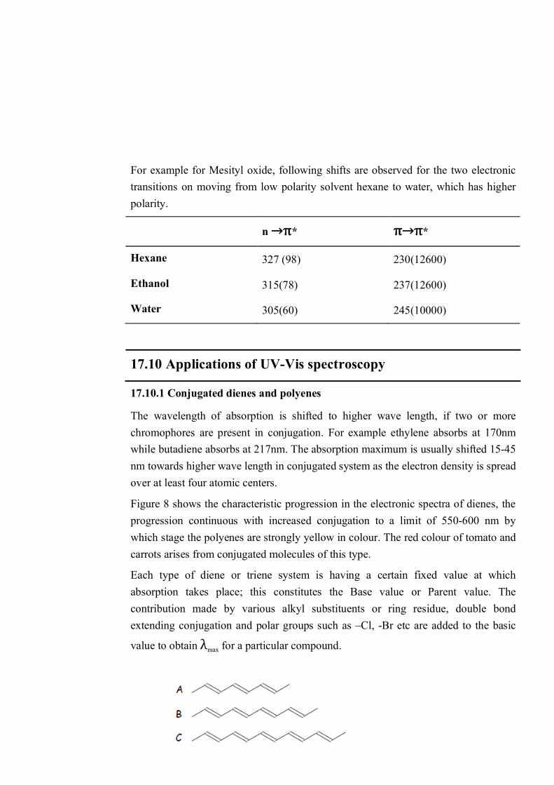
357

For example for Mesityl oxide, following shifts are observed for the two electronic transitions on moving from low polarity solvent hexane to water, which has higher polarity.

n →π* π→π*

Hexane 327 (98) 230(12600)

Ethanol 315(78) 237(12600)

Water 305(60) 245(10000)

17.10 Applications of UV-Vis spectroscopy

17.10.1 Conjugated dienes and polyenes

The wavelength of absorption is shifted to higher wave length, if two or more chromophores are present in conjugation. For example ethylene absorbs at 170nm while butadiene absorbs at 217nm. The absorption maximum is usually shifted 15-45 nm towards higher wave length in conjugated system as the electron density is spread over at least four atomic centers.

Figure 8 shows the characteristic progression in the electronic spectra of dienes, the progression continuous with increased conjugation to a limit of 550-600 nm by which stage the polyenes are strongly yellow in colour. The red colour of tomato and carrots arises from conjugated molecules of this type.

Each type of diene or triene system is having a certain fixed value at which absorption takes place; this constitutes the Base value or Parent value. The contribution made by various alkyl substituents or ring residue, double bond extending conjugation and polar groups such as –Cl, -Br etc are added to the basic

value to obtain λmax for a particular compound.

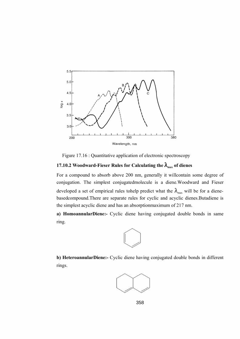
358

Figure 17.16 : Quantitative application of electronic spectroscopy

17.10.2 Woodward-Fieser Rules for Calculating the λmax of dienes

For a compound to absorb above 200 nm, generally it willcontain some degree of conjugation. The simplest conjugatedmolecule is a diene.Woodward and Fieser

developed a set of empirical rules tohelp predict what the λmax will be for a diene-basedcompound.There are separate rules for cyclic and acyclic dienes.Butadiene is the simplest acyclic diene and has an absorptionmaximum of 217 nm.

a) HomoannularDiene:- Cyclic diene having conjugated double bonds in same ring.

b) HeteroannularDiene:- Cyclic diene having conjugated double bonds in different rings.

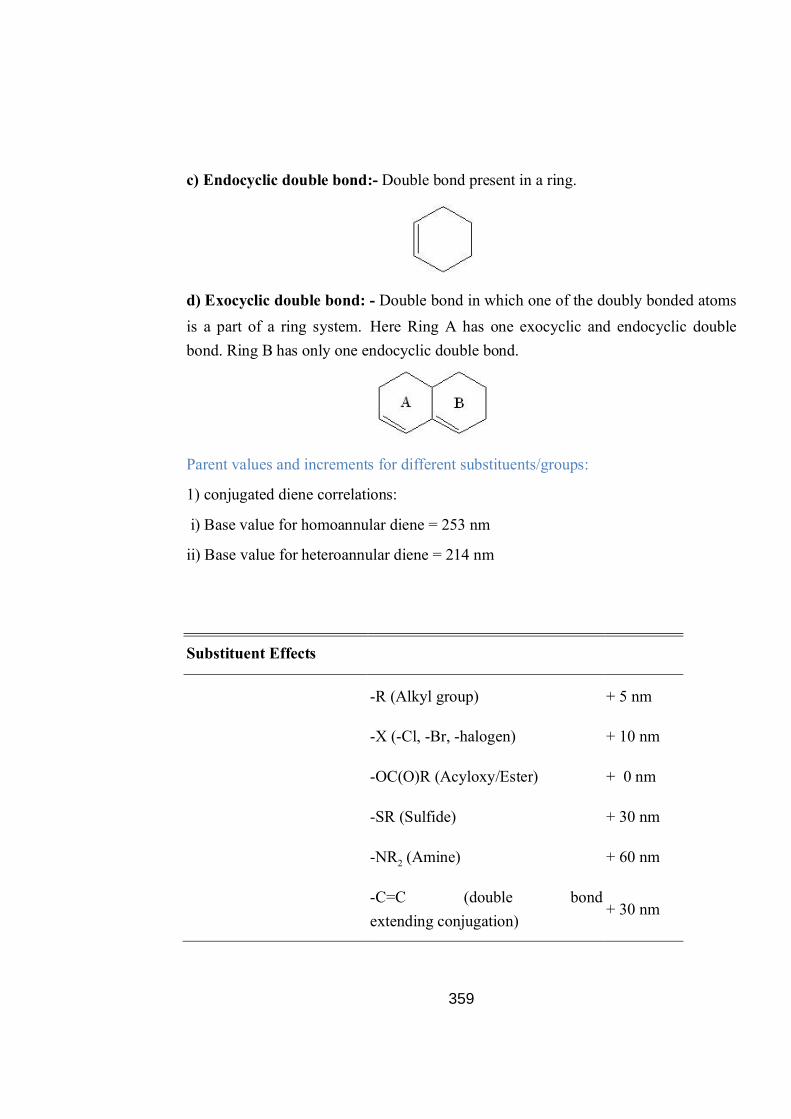
359

c) Endocyclic double bond:- Double bond present in a ring.

d) Exocyclic double bond: - Double bond in which one of the doubly bonded atoms is a part of a ring system. Here Ring A has one exocyclic and endocyclic double bond. Ring B has only one endocyclic double bond.

Parent values and increments for different substituents/groups:

1) conjugated diene correlations:

i) Base value for homoannular diene = 253 nm

ii) Base value for heteroannular diene = 214 nm

Substituent Effects

-R (Alkyl group) + 5 nm

-X (-Cl, -Br, -halogen) + 10 nm

-OC(O)R (Acyloxy/Ester) + 0 nm

-SR (Sulfide) + 30 nm

-NR2 (Amine) + 60 nm

-C=C (double bond extending conjugation)

+ 30 nm

360

- C6H5 (Phenyl group) + 60 nm

- Exocyclic double bond + 5 nm

Examples

214 (base value) + 5 (one alkyl group) = 219 nm

214 (base value) + 30(one conjugated DB) = 244 nm

214 (base value) + 5x2 (two alkyl groups) + 5 (one exocyclic

DB) = 229 nm

214 (base value) + 5x3 (three alkyl groups) + 5 (one exocyclic

DB) = 234 nm

214 (base value) + 5x2 (two alkyl groups) = 224 nm

253 (base value) + 5x6 (six alkyl groups) + 30 (one conjugated DB) + 5 (one exocyclic DB) = 318 nm

For X = EtO

215 (base value) + 5x3 (three alkyl groups) + 5 (one exocyclic DB) + 6 (one OR group) = 241 nm

For X = MeS

215 (base value) + 5x3 (three alkyl groups) + 5 (one exocyclic DB) + 30 (one SR group) = 265 nm

For X = Br

X

361

215 (base value) + 5x3 (three alkyl groups) + 5 (one exocyclic DB) + 5 (one Br group) = 240 nm

17.10.3 Woodward-Fieser Rules for Calculating the λmax of Polyenes

The Woodward’s rules work well only for conjugated polyenes having four double bonds or less. For conjugated polyenes with more than four double bonds the Fieser- Kuhn rules are used.

λmax= 114 + 5M + n (48 - 1.7n) – 16.5 Rendo-10 Rexo

where

n = no. of conjugated double bonds

M = no. of alkyl groups

Rendo = no. of endocyclic double bonds

Rexo = no. of exocyclic double bonds

For example calculated λmax in lycopene and beta caroteneis:

λmax(cal) = 114 + 5(8) + 11(48-1.7.11) - 0 - 0 = 476 nm

λmax(actual) = 474

λmax(cal) = 114 + 5(10) + 11(48-1.7.11) - 16.5(2) - 0 = 453.3 nm

λmax(actual) = 452

362

λmax(cal) = 114 + 5(8) + 11(48-1.7.11) - 16.5(0) - 10(0) = 486.3 nm

λmax(cal) = 114 + 5(6) + 7(48-1.7*7) - 16.5(0) - 10(0) = 396.7 nm

17.10.4 UV absorption in Conjugated Carbonyl Compounds

In conjugated carbonyl compounds where the double bond and the carbonyl groups

are in conjugation. Both n →π* and π→π* show bathochromic shifts. Unsaturated carbonyl compounds show slightly stronger band or series of bands in the 300-350 nm range. The positions as well as intensity of bands are influenced by transannular interactions and also by solvents. By increasing the polarity of solvent experience a red shift while transition undergoes a blue shift. The changing polarity of solvent brings about a change in energy difference between the levels involved in the transitions.

By comparing the UV spectra of unconjugated and conjugated carbonyl compounds bathochromic effect was observed.

17.10.5 Woodward-Fieser Rules for Calculating the λmax of Conjugated Carbonyl Compounds

Woodward-Fieser rules can be extended to calculate the λmax of α,β-unsaturated carbonyl compounds. In a similar manner to Woodward rules for dienes discussed previously, there is base value to which the substituent effects can be added and the

λmax can be calculated using the formula:

λmax = Base value + Σ Substituent Contributions + Σ Other Contributions

1. Base value:

O

OH

OH

O

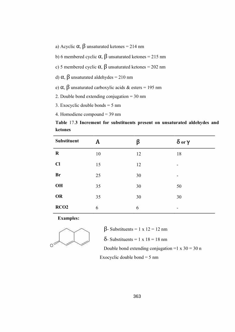
363

a) Acyclic α, β unsaturated ketones = 214 nm

b) 6 membered cyclic α, β unsaturated ketones = 215 nm

c) 5 membered cyclic α, β unsaturated ketones = 202 nm

d) α, β unsaturated aldehydes = 210 nm

e) α, β unsaturated carboxylic acids & esters = 195 nm

2. Double bond extending conjugation = 30 nm

3. Exocyclic double bonds = 5 nm

4. Homodiene compound = 39 nm

Table 17.3 Increment for substituents present on unsaturated aldehydes and ketones

Substituent Α β δ or γ

R 10 12 18

Cl 15 12 -

Br 25 30 -

OH 35 30 50

OR 35 30 30

RCO2 6 6 -

Examples:

β- Substituents = 1 x 12 = 12 nm

δ- Substituents = 1 x 18 = 18 nm

Double bond extending conjugation =1 x 30 = 30 n

Exocyclic double bond = 5 nm

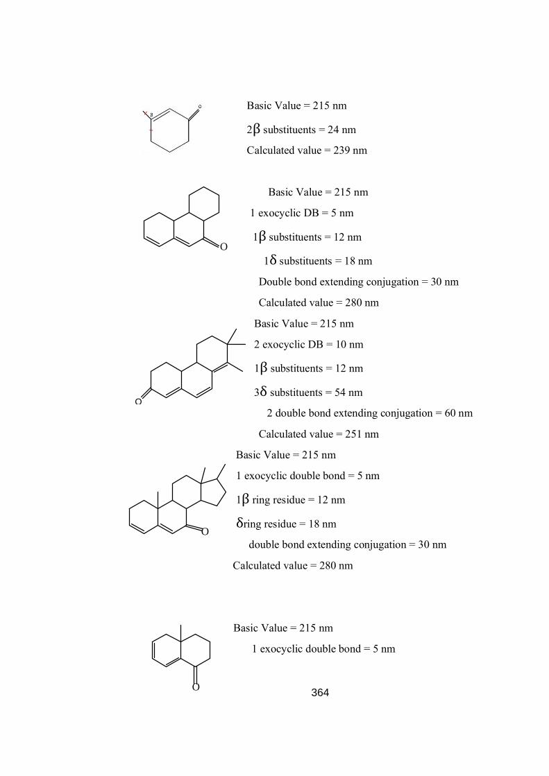
364

Basic Value = 215 nm

2β substituents = 24 nm

Calculated value = 239 nm


1 exocyclic DB = 5 nm


1δ substituents = 18 nm

Double bond extending conjugation = 30 nm



2 exocyclic DB = 10 nm


3δ substituents = 54 nm

2 double bond extending conjugation = 60 nm



1 exocyclic double bond = 5 nm

1β ring residue = 12 nm

δring residue = 18 nm

double bond extending conjugation = 30 nm



1 exocyclic double bond = 5 nm

O

O

O

O

365

α alkyl group = 12 nm

δalkyl group = 18 nm


1homoannular ring add = 39


Basic value =215


exocyclic double bond = 5 nm

1αsubstituent =12 nm

1 βsubstituent =18 nm

Calulated value = 298 nm

17.10.6 Woodward-Fieser Rules for Calculating the λmax of Aromatic Compounds

Base value

1. ArCOR = 246 nm 2. ArCHO = 250 nm 3. ArCOOH = 230 nm 4. ArCOOR = 230 nm

Substituent O m P

Alkyl 3 3 10

-OH, -CH3, -o alkyl 7 7 25

-Cl 0 0 10

-Br 2 2 15

-NH2 13 13 58

-NHCOCH3 20 20 45

366

-N(CH3)2 20 20 85

Examples:

Base value =246 nm

Ring residue in o- position = 1 x 3 = 3 nm

Polar group -OCH3 in p- position = 25 nm


Base value =246 nm

Cl at para position = 1 x 3 = 3 nm


Observed value = 254 nm

Base value =246 nm

Br at meta position = 2 nm

0- ring residue = 3 nm


Observed value = 253 nm

(17.2) state True/ False in following

a) Electronic>Evibrutional >Erotatrational (T/F).

b) n π* trasition require more energy as compared to ҇҇ -- * transition (T/F).

c) uneconjugated alkenes absort at relationship between also rebalance and can

centation of also rebling species (T/F).

17.3 Complete the following:--

C

O

CH3

Cl

Br

O

367

a) Absorbanee = Σ-----------------.

b) Diene Lawing conjugated double bond in the different cydie ring is -----------

.c) A max = + Σ subsitutent contribution + Σ other contribution.

d) Base value for exocydie double bond=--------------- nm.

17.11Summary

UV/Vis spectroscopy is routinely used in analytical chemistry for the quantitative determination of different analytes, such as transition metal ions, highly conjugated organic compounds, and biological macromolecules. Spectroscopic analysis is commonly carried out in solutions but solids and gases may also be studied.

Solutions of transition metal ions can be colored (i.e., absorb visible light) because d electrons within the metal atoms can be excited from one electronic state to another. The colour of metal ion solutions is strongly affected by the presence of other species, such as certain anions or ligands. For instance, the colour of a dilute solution of copper sulfate is a very light blue; adding ammonia intensifies the colour and changes the wavelength of maximum absorption ( ).

Organic compounds, especially those with a high degree of conjugation, also absorb light in the UV or visible regions of the electromagnetic spectrum. The solvents for these determinations are often water for water-soluble compounds, or ethanol for organic-soluble compounds. (Organic solvents may have significant UV absorption; not all solvents are suitable for use in UV spectroscopy. Ethanol absorbs very weakly at most wavelengths.) Solvent polarity and pH can affect the absorption spectrum of an organic compound. Tyrosine, for example, increases in absorption maxima and molar extinction coefficient when pH increases from 6 to 13 or when solvent polarity decreases.

While charge transfer complexes also give rise to colours, the colours are often too intense to be used for quantitative measurement.

368

The Beer-Lambert law states that the absorbance of a solution is directly proportional to the concentration of the absorbing species in the solution and the path length. Thus, for a fixed path length, UV/Vis spectroscopy can be used to determine the concentration of the absorber in a solution. It is necessary to know how quickly the absorbance changes with concentration. This can be taken from references (tables of molar extinction coefficients), or more accurately, determined from a calibration curve.

A UV/Vis spectrophotometer may be used as a detector for HPLC. The presence of an analyte gives a response assumed to be proportional to the concentration. For accurate results, the instrument's response to the analyte in the unknown should be compared with the response to a standard; this is very similar to the use of calibration curves. The response (e.g., peak height) for a particular concentration is known as the response factor.

The wavelengths of absorption peaks can be correlated with the types of bonds in a given molecule and are valuable in determining the functional groups within a molecule. The Woodward-Fieser rules, for instance, are a set of empirical

observations used to predict λmax, the wavelength of the most intense UV/Vis absorption, for conjugated organic compounds such as diene and ketones. The spectrum alone is not, however, a specific test for any given sample. The nature of the solvent, the pH of the solution, temperature, high electrolyte concentrations, and the presence of interfering substances can influence the absorption spectrum. Experimental variations such as the slit width (effective bandwidth) of the spectrophotometer will also alter the spectrum. To apply UV/Vis spectroscopy to analysis, these variables must be controlled or accounted for in order to identify the substances present

Although UV-visible spectra do not enable absolute identification of an unknown compound, UV spectra and Visible spectra can be used to identify a compound by comparative analysis. One can compare the UV or Visible spectra of the unknown with the spectra of known suspects.

Besides detecting the presence of distinctive chromophores in a molecule, UV/VIS spectroscopy can also be used to use to detect the extent of conjugation in a molecule, more the conjugation the longer the wavelength of absorption. Each additional double bond in the conjugated pi-electron system shifts the absorption

369

maximum about 30 nm towards longer wavelength. This is due to decreasing energy gap between HOMO and LUMO as the conjugation increases.

UV/vis spectroscopy can also use be used to study geometric isomerism of molecules. The trans isomer absorbs at longer wavelength with a larger molar extinction constant than cis isomer. This can be explained by the steric strain

introduced in the cis isomer resulting in lesser π orbital overlap.

UV/Vis spectroscopy can also be used to study the degree of strain; the degree of conjugation may suffer in strained molecules (e.g 2-substitued biphenyls) by correlating changes in spectrum with angular distortion. It can also be used to distinguish the most stable tautomeric forms. The UV spectrum of the solution will be found to be complimentary to more abundant tautomer.

The equilibrium has been shown to lie far to the right, i.e., the UV spectrum of the solution resembles that of the prid-2-one rather than 2-hydroxy pyridine.

17.12 Glossary

Chromophone:-- Any esolated covalently bonded grorup that shous a

chavaterlistee absortion in UV region

Aukchrome :-- a group whose pressure lurning about a shift of the absortion land

towards red end of specter .

Batho chromine shift:-- Absorption maximum is shifted towards longer waluding.


1. Applying Woodward-Fieser rules, calculate the values of absorption maxima for the following compounds.

O Br

OCH3

O

COOC2H5

Cl

CH2OH

CH3

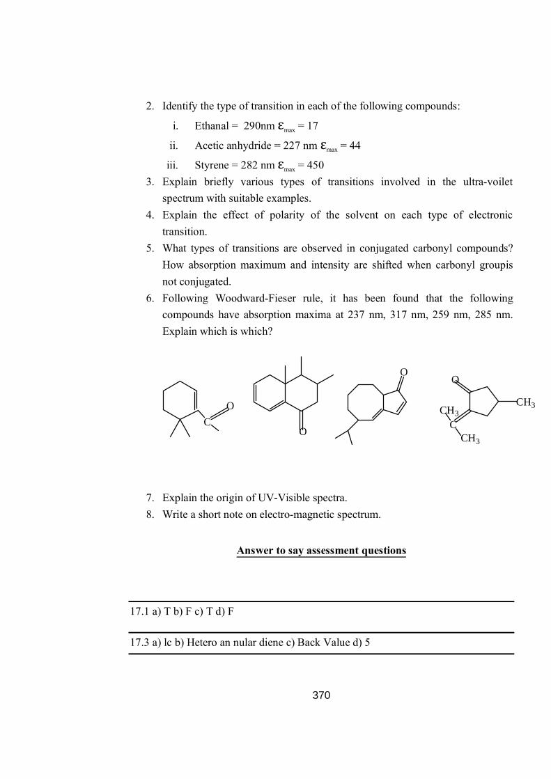
370

2. Identify the type of transition in each of the following compounds:

i. Ethanal = 290nm εmax = 17

ii. Acetic anhydride = 227 nm εmax = 44

iii. Styrene = 282 nm εmax = 450 3. Explain briefly various types of transitions involved in the ultra-voilet

spectrum with suitable examples. 4. Explain the effect of polarity of the solvent on each type of electronic

transition. 5. What types of transitions are observed in conjugated carbonyl compounds?

How absorption maximum and intensity are shifted when carbonyl groupis not conjugated.

6. Following Woodward-Fieser rule, it has been found that the following compounds have absorption maxima at 237 nm, 317 nm, 259 nm, 285 nm. Explain which is which?

7. Explain the origin of UV-Visible spectra. 8. Write a short note on electro-magnetic spectrum.


17.1 a) T b) F c) T d) F

17.3 a) lc b) Hetero an nular diene c) Back Value d) 5

CO

O

O

O

CCH3

CH3

CH3

371


1. Donald L. Pavia, Gary M. Lampman, George S. kriz, James R. Vyvyan, Spectroscopy, Cengage Learning India Pvt. Ltd., 2011.

2. Y.R. Sharma, Elementry Organic Spectroscopy, S. Chand & Company Ltd., New Delhi, 2011.

3. I. Fleming and D.H. William, Spectroscopic Methods in Organic Chemistry, Mc-Graw Hill, 1973.

4. Work book of Fundamentals of UV-Visible Spectroscopy, Agilent Technologies, 2000.

372

Unit – 18 : Infrared spectroscopy Structure of unit

18.0 Objective

18.1 Introduction

18.2 Infrared spectroscopy

18.3 Condition for absorption of Infrared radiation

18.4 Molecular Vibrations

18.5 The Harmonic Oscillator

18.6 Anharmonic oscillator

18.7 Vibrational Spectra of Di and poly-atomic molecule

18.8 Nuclear spin effect

18.9 Uses and applications

18.10 Summary

18.11 Glossary

Aswer to key assessment questions


18.12 References and suggested readings

18.0 Objective

At the end of the unit learner will be able to understand

What is Infrared Spectroscopy?

Absorption of IR and Molecular Vibration.

Harmonic and anharmonic oscillator.

Nuclear spin effects and applications of IR.

18.1 Introduction

This unit deals with the analytical aspects of IR spectroscopy its use and applicataions in different fields of investigation. This unit gives detailed description

373

about vibrational spectroscopy and vibrational spectra, harmonic and anharmonic oscillator, alongwith these vibratioal spectra of di and poly atomic molecules are also discussed.

18.2 Infrared spectroscopy

Difination: Infrared spectroscopy (IR spectroscopy) is the spectroscopy that deals with the infrared region of the electromagnetic spectrum, which is light with a longer wavelength and lower frequency than visible light. It covers a range of techniques, mostly based on absorption spectroscopy. As with all spectroscopic techniques, it can be used to identify and study chemicals. A common laboratory instrument that uses this technique is a Fourier transform infrared (FTIR) spectrometer.

Infrared (IR) light is electromagnetic radiation with longer wavelengths than those of visible light, extending from the nominal red edge of the visible spectrum at 700 nanometers (nm) to 1 mm. This range of wavelengths corresponds to a frequency range of approximately 430 THz down to 300 GHz. Most of the thermal radiation emitted by objects near room temperature is infrared.

Infrared spectroscopy is part of vibrational spectroscopy. It is a technique that can be used to identify molecules by analysis of their constituent bonds. Each chemical bond in a molecule vibrates at a frequency characteristic of that bond. A group of atoms in a molecule (e.g., CH2) may have multiple modes of oscillation caused by the stretching and bending motions of the group as a whole. If an oscillation leads to a change in dipole in the molecule then it will absorb a photon that has the same frequency. The vibrational frequencies of most molecules correspond to the frequencies of infrared light. Typically, the technique is used to study organic compounds using light radiation from 4000–400 cm−1, the mid-infrared. A spectrum of all the frequencies of absorption in a sample is recorded. This can be used to gain information about the sample composition in terms of chemical groups present and also its purity (for example, a wet sample will show a broad O-H absorption around 3200 cm−1).

Infrared spectroscopy exploits the fact that molecules absorb specific frequencies that are characteristic of their structure. These absorptions are resonant frequencies, i.e. the frequency of the absorbed radiation matches the transition energy of the bond or group that vibrates. The energies are determined by the shape of the molecular

374

potential energy surfaces, the masses of the atoms, and the associated vibronic coupling.

Infrared light is emitted or absorbed by molecules when they change their rotational-vibrational movements. Infrared energy elicits vibrational modes in a molecule through a change in the dipole moment, making it a useful frequency range for study of these energy states for molecules of the proper symmetry. Infrared spectroscopy examines absorption and transmission of photons in the infrared energy range.

The infrared range of electromagnetic spectrum is usually divided into three regions; the near-, mid- and far- infrared, named for their relation to the visible spectrum.

1.The higher-energy near-IR, approximately 14000–4000 cm−1 (0.8–2.5 μm wavelength) can excite overtone or harmonic vibrations.

2.The mid-infrared, approximately 4000–400 cm−1 (2.5–25 μm) may be used to study the fundamental vibrations and associated rotational-vibrational structure.

3.The far-infrared, approximately 400–10 cm−1 (25–1000 μm), lying adjacent to the microwave region, has low energy and may be used for rotational spectroscopy.

The names and classifications of these subregions are conventions, Fig 18.1and are only loosely based on the relative molecular or electromagnetic properties.

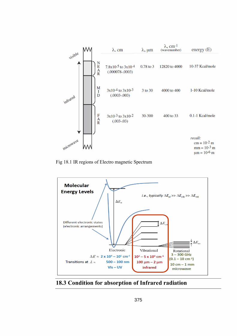
375

Fig 18.1 IR regions of Electro magnetic Spectrum

18.3 Condition for absorption of Infrared radiation

376

In order for molecular vibrations to absorb IR energy, the vibrational motions must change the dipole moment of the molecule. All molecules with three or more atoms meet this criterion and are IR absorbers.

The absorptions by CO2:

All molecules have positive (nuclei) and negative (electron clouds) regions, A molecule is dipolar and has a permanent dipole moment, if the averaged centers of its positively and negatively charged regions do not coincide. If a vibrational motion of the molecule disturbs these averages, its dipole moment can change and an appropriate energy of IR radiation can be absorbed to cause this molecular vibration. As an example, consider the CO2 molecule. The more electronegative oxygen atoms attract electron density that makes the ends of the molecule slightly negative. The central carbon atom is therefore slightly positive, as represented in the diagram. Since the molecule is linear with equal bond lengths, the center of negative charge and the center of positive charge coincide at the central point, the carbon atom, and the molecule has no permanent dipole moment. The symmetrical stretching vibration, top representation, does not change this symmetry, does not change the dipole moment, and does not lead to IR absorption. The molecular bending vibrations, middle two representations, displace the negative charges away from the line of centers of the molecule and create a structure with a dipole moment. Thus, the dipole moment changes (from zero to some value) and these motions can be initiated by the absorption of IR radiation.

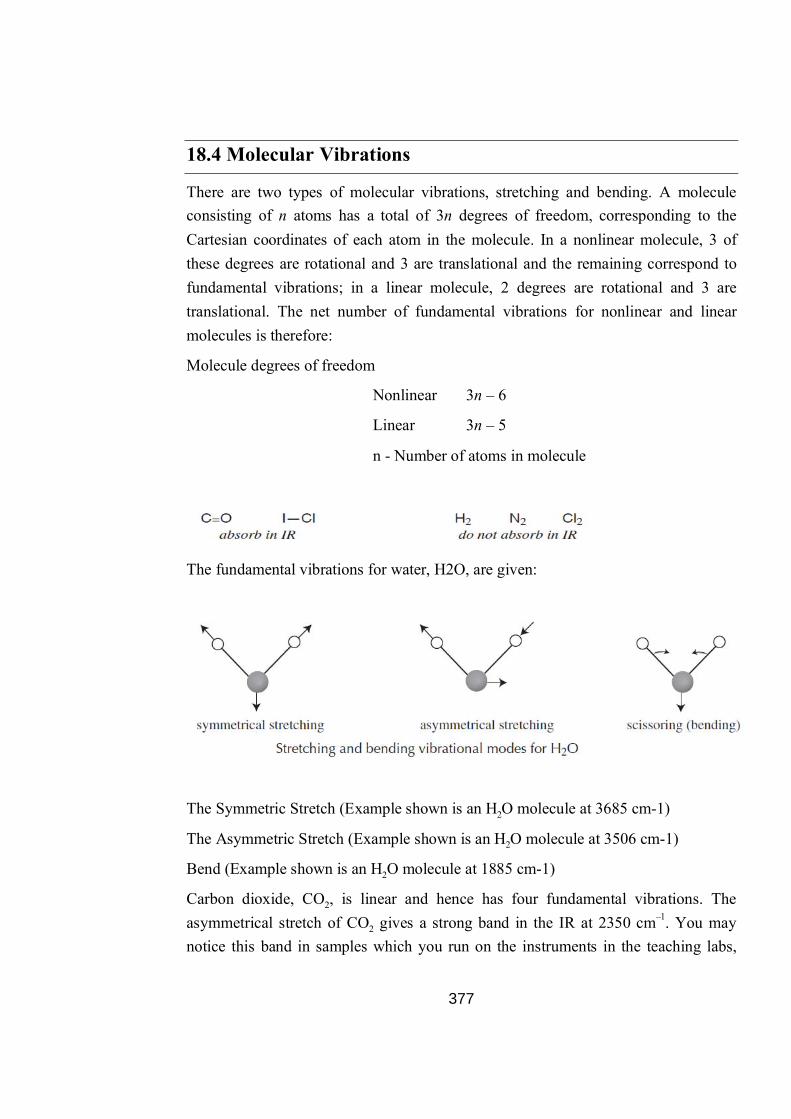
377

18.4 Molecular Vibrations

There are two types of molecular vibrations, stretching and bending. A molecule consisting of n atoms has a total of 3n degrees of freedom, corresponding to the Cartesian coordinates of each atom in the molecule. In a nonlinear molecule, 3 of these degrees are rotational and 3 are translational and the remaining correspond to fundamental vibrations; in a linear molecule, 2 degrees are rotational and 3 are translational. The net number of fundamental vibrations for nonlinear and linear molecules is therefore:

Molecule degrees of freedom

Nonlinear 3n – 6

Linear 3n – 5

n - Number of atoms in molecule

The fundamental vibrations for water, H2O, are given:

The Symmetric Stretch (Example shown is an H2O molecule at 3685 cm-1)

The Asymmetric Stretch (Example shown is an H2O molecule at 3506 cm-1)

Bend (Example shown is an H2O molecule at 1885 cm-1)

Carbon dioxide, CO2, is linear and hence has four fundamental vibrations. The asymmetrical stretch of CO2 gives a strong band in the IR at 2350 cm–1. You may notice this band in samples which you run on the instruments in the teaching labs,

378

since CO2 is present in the atmosphere. The two scissoring or bending vibrations are equivalent and therefore, have the same frequency and are said to be degenerate, appearing in an IR spectrum at 666 cm–1. The symmetrical stretch of CO2 is inactive in the IR because this vibration produces no change in the dipole moment of the molecule. In order to be IR active, a vibration must cause a change in the dipole moment of the molecule. Of the following linear molecules, carbon monoxide and iodine chloride absorb IR radiation, while hydrogen, nitrogen, and chlorine do not. In general, the larger the dipole change, the stronger the intensity of the band in an IR spectrum.

Only two IR bands (2350 and 666 cm–1) are seen for carbon dioxide, instead of four corresponding to the four fundamental vibrations. Carbon dioxide is an example of why one does not always see as many bands as implied by our simple calculation. In the case of CO2, two bands are degenerate, and one vibration does not cause a change in dipole moment. Other reasons why fewer than the theoretical number of IR bands are seen include: an absorption is not in the 4000–400 cm–1 range; an absorption is too weak to be observed; absorptions are too close to each other to be resolved on the instrument. Additional weak bands which are overtones or combinations of fundamental vibrations are observed.

Stretching Vibrations

The stretching frequency of a bond can be approximated by Hooke’s Law. In this approximation, two atoms and the connecting bond are treated as a simple harmonic oscillator composed of 2 masses (atoms) joined by a spring:

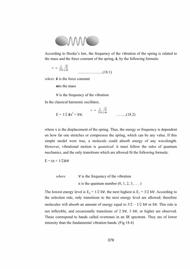
379

According to Hooke’s law, the frequency of the vibration of the spring is related to the mass and the force constant of the spring, k, by the following formula:

………………..(18.1)

where k is the force constant

mis the mass

ν is the frequency of the vibration

In the classical harmonic oscillator,

E = 1/2 kx2 = hν, ……..(18.2)

where x is the displacement of the spring. Thus, the energy or frequency is dependent on how far one stretches or compresses the spring, which can be any value. If this simple model were true, a molecule could absorb energy of any wavelength. However, vibrational motion is quantized: it must follow the rules of quantum mechanics, and the only transitions which are allowed fit the following formula:

E = (n + 1/2)hν

where ν is the frequency of the vibration

n is the quantum number (0, 1, 2, 3, . . . )

The lowest energy level is E0 = 1/2 hν, the next highest is E1 = 3/2 hν. According to the selection rule, only transitions to the next energy level are allowed; therefore

molecules will absorb an amount of energy equal to 3/2 – 1/2 hν or hν. This rule is

not inflexible, and occasionally transitions of 2 hν, 3 hν, or higher are observed. These correspond to bands called overtones in an IR spectrum. They are of lower intensity than the fundamental vibration bands. (Fig 18.4)

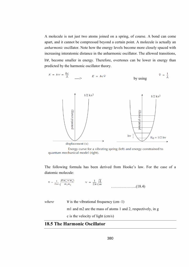
380

A molecule is not just two atoms joined on a spring, of course. A bond can come apart, and it cannot be compressed beyond a certain point. A molecule is actually an anharmonic oscillator. Note how the energy levels become more closely spaced with increasing interatomic distance in the anharmonic oscillator. The allowed transitions,

hν, become smaller in energy. Therefore, overtones can be lower in energy than predicted by the harmonic oscillator theory.

----> by using

The following formula has been derived from Hooke’s law. For the case of a diatomic molecule:

………………..(18.4)

where ν is the vibrational frequency (cm–1)

m1 and m2 are the mass of atoms 1 and 2, respectively, in g

c is the velocity of light (cm/s)

18.5 The Harmonic Oscillator

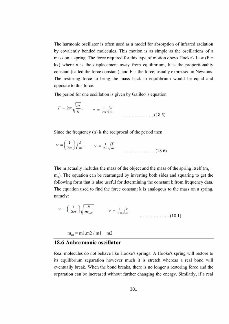
381

The harmonic oscillator is often used as a model for absorption of infrared radiation by covalently bonded molecules. This motion is as simple as the oscillations of a mass on a spring. The force required for this type of motion obeys Hooke's Law (F = kx) where x is the displacement away from equilibrium, k is the proportionality constant (called the force constant), and F is the force, usually expressed in Newtons. The restoring force to bring the mass back to equilibrium would be equal and opposite to this force.

The period for one oscillation is given by Galileo' s equation

………………..(18.5)

Since the frequency (n) is the reciprocal of the period then

………………..(18.6)

The m actually includes the mass of the object and the mass of the spring itself (m1 + m2). The equation can be rearranged by inverting both sides and squaring to get the following form that is also useful for determining the constant k from frequency data. The equation used to find the force constant k is analogous to the mass on a spring, namely:

………………..(18.1)

meff = m1.m2 / m1 + m2

18.6 Anharmonic oscillator

Real molecules do not behave like Hooke's springs. A Hooke's spring will restore to its equilibrium separation however much it is stretch whereas a real bond will eventually break. When the bond breaks, there is no longer a restoring force and the separation can be increased without further changing the energy. Similarly, if a real

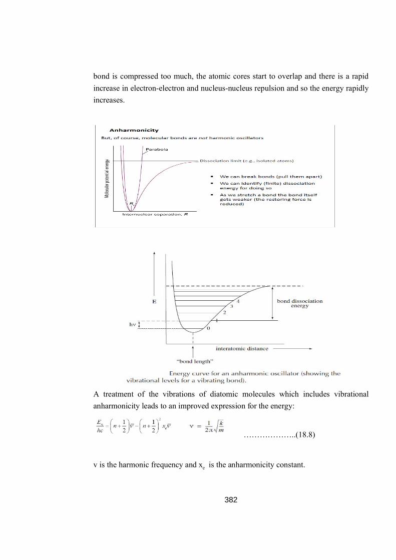
382

bond is compressed too much, the atomic cores start to overlap and there is a rapid increase in electron-electron and nucleus-nucleus repulsion and so the energy rapidly increases.

A treatment of the vibrations of diatomic molecules which includes vibrational anharmonicity leads to an improved expression for the energy:

………………..(18.8)

v is the harmonic frequency and xe is the anharmonicity constant.

383

18.7 Vibrational Spectra of Di and poly-atomic molecule

A molecule with N atoms has a total of 3N degrees of freedom for its nuclear motions, since each nucleus can be independently displaced in three perpendicular directions. Three of these degrees of freedom correspond to translational motion of the center of mass. For a nonlinear molecule, three more degrees of freedom determine the orientation of the molecule in space, and thus its rotational motion. This leaves 3N-6 vibrational modes. For a linear molecule, there are just two rotational degrees of freedom, which leaves 3N-5 vibrational modes. A diatomic molecule has one normal mode of vibration. The normal modes of vibration of polyatomic molecules are independent of each other but each normal mode will involve simultaneous vibrations of different parts of the molecule such as different chemical bonds. For example, the nonlinear molecule H2O has three vibrational modes while the linear molecule CO2 has four vibrational modes. The vibrations consist of coordinated motions of several atoms in such a way as to keep the center of mass stationary and nonrotating. These are called the normal modes. Each normal mode has a characteristic resonance frequency, which is usually determined experimentally. To a reasonable approximation, each normal mode behaves as an independent harmonic oscillator of frequency. The normal modes of H2O and CO2 are pictured below. (Fig 18.6 and 18.7)

Fig 18.6 Normal modes of vibrations of H2O

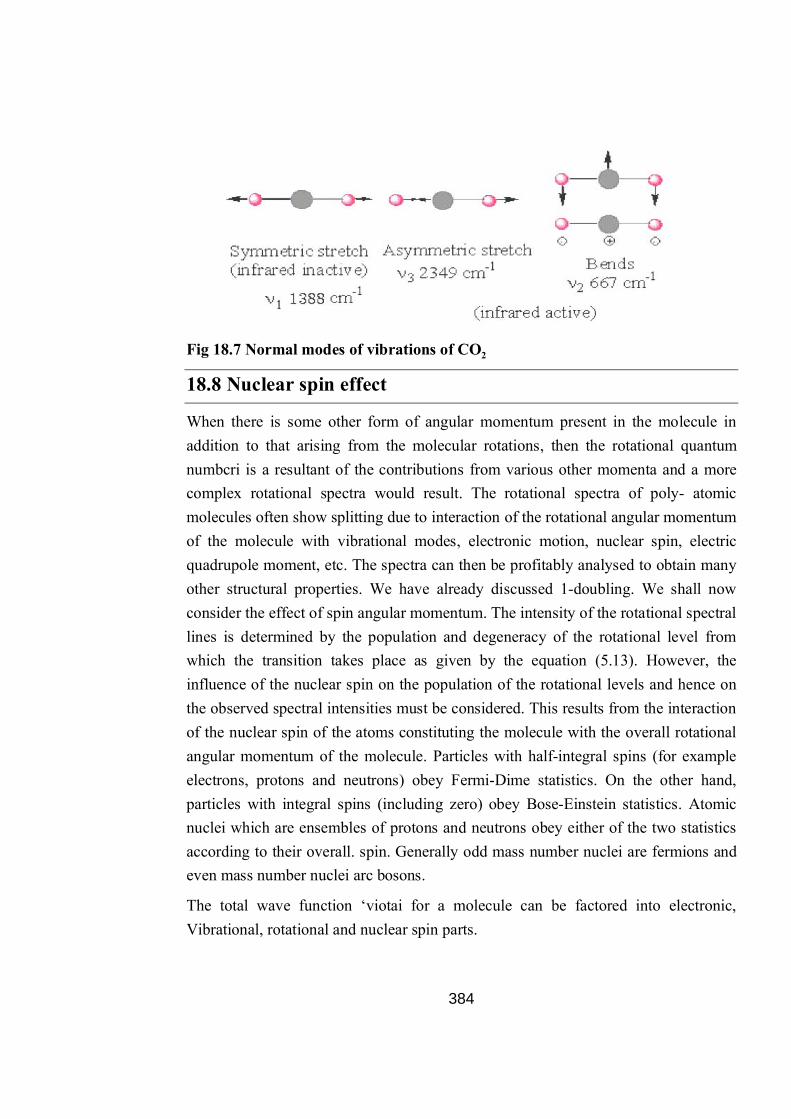
384

Fig 18.7 Normal modes of vibrations of CO2

18.8 Nuclear spin effect

When there is some other form of angular momentum present in the molecule in addition to that arising from the molecular rotations, then the rotational quantum numbcri is a resultant of the contributions from various other momenta and a more complex rotational spectra would result. The rotational spectra of polyatomic molecules often show splitting due to interaction of the rotational angular momentum of the molecule with vibrational modes, electronic motion, nuclear spin, electric quadrupole moment, etc. The spectra can then be profitably analysed to obtain many other structural properties. We have already discussed 1-doubling. We shall now consider the effect of spin angular momentum. The intensity of the rotational spectral lines is determined by the population and degeneracy of the rotational level from which the transition takes place as given by the equation (5.13). However, the influence of the nuclear spin on the population of the rotational levels and hence on the observed spectral intensities must be considered. This results from the interaction of the nuclear spin of the atoms constituting the molecule with the overall rotational angular momentum of the molecule. Particles with half-integral spins (for example electrons, protons and neutrons) obey Fermi-Dime statistics. On the other hand, particles with integral spins (including zero) obey Bose-Einstein statistics. Atomic nuclei which are ensembles of protons and neutrons obey either of the two statistics according to their overall. spin. Generally odd mass number nuclei are fermions and even mass number nuclei arc bosons.

The total wave function ‘viotai for a molecule can be factored into electronic, Vibrational, rotational and nuclear spin parts.

385

In a homonuclcar molecule, that is, in a ccntrosymmetric molecule, the total wave function 1v(aI should be symmetric with respect to exchange of nuclei (say under a C’2 symmetry operation) if the nuclei have integral spins (bosons) and antisymnictric with respect to exchange of nuclei if the nuclei have half integral spins (fermions). For molecules with zero total orbital angular momentum, the electronic and vibrational wave functions in their ground state arc symmetric. The basic symmetry property of the rotational levels is such that the even J levels (J 0, 2,4 ) arc symmetric and the oddJlcvcls (J 1,3, 5,...) arc antisymrnctric. Thus the rotational wave functions with even Jdo not change sign under exchange of nuclei while functions with odd Jdo so. This is easy to see, since the rotational wave functions are just the same Lcgcndrc polynomials that describe the angular part of the hydrogen atom wave functions.For a nucleus of spin fin a molecule, of the possible (2I + 1)2 nuclear spin states, (2I + I )(I+1) arc symmetric and (2I+1 )(I) arc antisymmetric. In a diatomic molecule, each of these atoms is in a particular electronic state. In the study of the spectroscopy of the diatomic molecules, the molecular states that are formed from a given pair of atoms are required.

ψtotal= ψelectron + ψvibrational + ψrotational + ψnuclear spin ……..(18.1)

18.9 Uses and applications

Analytical Information

Qualitative

The combination of the fundamental vibrations or rotations of various functional groups and the interactions of these functional groups with other atoms of the molecule results in the unique, generally complex IR spectrum for each individual compound. IR spectroscopy is mainly used in two ways: structural elucidation and compound identification.

Structural Elucidation: Because of complex interactions of atoms within the molecule, IR absorption of the functional groups may vary over a wide range. However, it has been found that many functional groups give characteristic peaks.

Compound Identification: Since the IR spectrum of every molecule is unique, one of the most positive identification methods of an organic compound is to find a

386

reference IR spectrum that matches that of the unknown compound. A large number of reference spectra for vapor and condensed phases are available in printed and electronic formats. The spectral libraries compiled by Sadtler and Aldrich are some of the most popular collections. In addition, spectral databases are often compiled according to application areas such as forensics, biochemicals, and polymers

Quantitative

IR spectroscopy was generally considered to be able to provide only qualitative and semiquantitative analyses of common samples, especially when the data were acquired using the conventional dispersive instruments. However, the development of reliable FTIR instrumentation and strong computerized data-processing capabilities have greatly improved the performance of quantitative IR work. Thus, modern infrared spectroscopy has gained acceptance as a reliable tool for quantitative analysis.

1. Analysis of Petroleum Hydrocarbons, Oil, and Grease Contents

2. Quantitative Analysis of Multicomponent Mixtures of Sulfur Oxygen Anions by Attenuated Total Reflectance Spectroscopy.

3. Characterization of Heterogeneous Catalysts by Diffuse Reflectance Spectroscopy.

4. Qualitative Analysis of Multilayered Polymeric Films using FTIR Microspectroscopy.

Other applications

1. Infrared spectroscopy is a simple and reliable technique widely used in both organic and inorganic chemistry, in research and industry. It is used in quality control, dynamic measurement, and monitoring applications such as the long-term unattended measurement of CO2 concentrations in greenhouses and growth chambers by infrared gas analyzers.

2. It is also used in forensic analysis in both criminal and civil cases, for example in identifying polymer degradation. It can be used in detecting how much alcohol is in the blood of a suspected drunk driver measured as

1/10,000 g/mL = 100 μg/mL.

387

3. A useful way of analysing solid samples without the need for cutting samples uses ATR or attenuated total reflectance spectroscopy. Using this approach, samples are pressed against the face of a single crystal. The infrared radiation passes through the crystal and only interacts with the sample at the interface between the two materials.

4. With increasing technology in computer filtering and manipulation of the results, samples in solution can now be measured accurately (water produces a broad absorbance across the range of interest, and thus renders the spectra unreadable without this computer treatment).

5. Some instruments will also automatically tell you what substance is being measured from a store of thousands of reference spectra held in storage.

6. Infrared spectroscopy is also useful in measuring the degree of polymerization in polymer manufacture. Changes in the character or quantity of a particular bond are assessed by measuring at a specific frequency over time. Modern research instruments can take infrared measurements across the range of interest as frequently as 32 times a second. This can be done whilst simultaneous measurements are made using other techniques. This makes the observations of chemical reactions and processes quicker and more accurate.

7. Infrared spectroscopy has also been successfully utilized in the field of semiconductor microelectronics: for example, infrared spectroscopy can be applied to semiconductors like silicon, gallium arsenide, gallium nitride, zinc selenide, amorphous silicon, silicon nitride, etc.

8. The instruments are now small, and can be transported, even for use in field trials.

18.1 Fill in the blanks.

a) Rotational spectra show splitting due to interaction of _______momentum with

different modes.

b) For a lunieur moleaule there is _________ vibrational modes

388

c) IR radiation by covalently bounded molecules are model for ______ ascillatro.

d) the Stretchning frequency of a bond can be approximated by _________ low.

e) CO2 molecule has ________ fundamental vibration.

f) For TR Vibrational moleaule must show.

g)Higher TR region is in ______________ region.

h)According to Hookis low S=_--------------------------.

18.10 Summary

The ideas fundamental to an understanding of infrared spectroscopy were introduced in this chapter.

The electromagnetic spectrum was considered in terms of various atomic and molecular processes and classical and quantum ideas were introduced. The vibrations of molecules and how they produce infrared spectra were then examined.

The various factors that are responsible for the position and intensity of infrared modes were described.

An appreciation of these issues is important whenexamining spectra and these factors were outlined in this chapter.

18.11 Glossary.

Infrared light :-- Electromegnatic radiation with longer wavelength than

those of visible light.

Symmetric stretching :--- movement of the atom with the respect to a

particular atom in a maluale is in the same direction.

Rocking :-- Movement of the atom take place in the same direction.

389

Twisting:-- one of the atom moves up the plane and other move down the

plane with the respect to control atom.


18.1 a) rotational angular b) 3N-5 c) harmonie d) Hoockes e) 4 f) dipole moment g)

14000-4000 cm-1 h) 1/2 π√K/m


1. Explain vibration spectroscopy.

2. Discuss molecular vibrational modes.

3. Explain nuclear spin effect.

4. What are the main applications of IR spectroscopy?

5. Explain vibrational spectra of di and poly atomic molecules with suitable examples.

18.13 References and suggested readings

1. Wikipedia, the free encyclopedia en.wikipedia.org

2. r2 e:\files\courses\361-2lab\11labs\harmonic oscillator.docx

3. Vibrational Spectroscopy: Theory And Applications By D. N. Sathyanarayana

390

Unit – 19 : Raman spectroscopy Structure of Unit

19.0 Objective

19.1 Introduction

19.2 Raman Spectroscopy

19.3 Rotational Raman spectra

19.4 Vibrational raman spectra

19.5 Polarization of light and raman spectra

19.6 Structure ellucidation by IR and RAMAN

19.7 Applications

19.8 Summary

19.12 Glossary



19.10 References and suggested Readings

19.0 Objective


The phenomenon of Raman scattering.

The basics of raman spectroscopy.

Rotational and vibrational raman spectra.

Polarization of light and raman spectra.

Structure ellucidation by IR and RAMAN

Applicatios of Raman Spectroscopy.

391

19.1 Introduction

The phenomenon of Raman scattering of light was first potulated by Smekai in 1923 and first observed experimentally in 1928 by Raman and Krishnan. Raman scattering is most easily seen as the change in frequency for a small percentage of the intensity in a monochromatic beam as the result of coupling between the incident radiation and vibrational energy levels of molecules. A vibraional mode will be Raman active only when it changes the polariazbility of the molecule.

Raman spectroscopy is a spectroscopic technique used to observe vibrational, rotational, and other low-frequency modes in a system. It relies on inelastic scattering, or Raman scattering, of monochromatic light, usually from a laser in the visible, near infrared, or near ultraviolet range. The laser light interacts with molecular vibrations, phonons or other excitations in the system, resulting in the energy of the laser photons being shifted up or down. The shift in energy gives information about the vibrational modes in the system. Infrared spectroscopy yields similar, but complementary, information.

Typically, a sample is illuminated with a laser beam. Light from the illuminated spot is collected with a lens and sent through a monochromator. Wavelengths close to the laser line due to elastic Rayleigh scattering are filtered out while the rest of the collected light is dispersed onto a detector.

Spontaneous Raman scattering is typically very weak, and as a result the main difficulty of Raman spectroscopy is separating the weak inelastically scattered light from the intense Rayleigh scattered laser light. There are a number of advanced types of Raman spectroscopy, including surface-enhanced Raman, resonance Raman, tip-enhanced Raman, polarised Raman, stimulated Raman (analogous to stimulated emission), transmission Raman, spatially offset Raman, and hyper Raman.

19.2 Raman Spectroscopy

Principle

The Raman effect occurs when light impinges upon a molecule and interacts with the electron cloud and the bonds of that molecule. For the spontaneous Raman effect, which is a form of light scattering, a photon excites the molecule from the ground state to a virtual energy state. When the molecule relaxes it emits a photon and it returns to a different rotational or vibrational state. The difference in energy between

392

the original state and this new state leads to a shift in the emitted photon's frequency away from the excitation wavelength. The Raman effect, which is a light scattering phenomenon, should not be confused with absorption (as with fluorescence) where the molecule is excited to a discrete (not virtual) energy level.

If the final vibrational state of the molecule is more energetic than the initial state, the emitted photon will be shifted to a lower frequency for the total energy of the system to remain balanced. This shift in frequency is designated as a Stokes shift. If the final vibrational state is less energetic than the initial state, then the emitted photon will be shifted to a higher frequency, and this is designated as an anti-Stokes shift. Raman scattering is an example of inelastic scattering because of the energy transfer between the photons and the molecules during their interaction.

A change in the molecular polarization potential—or amount of deformation of the electron cloud—with respect to the vibrational coordinate is required for a molecule to exhibit a Raman effect. The amount of the polarizability change will determine the Raman scattering intensity. The pattern of shifted frequencies is determined by the rotational and vibrational states of the sample. This dependence on the polarizability differs from Infrared spectroscopy where the interaction between the molecule and light is determined by the dipole moment; this contrasting feature allows one to analyze transitions that might not be IR active via Raman spectroscopy, as exemplified by the rule of mutual exclusion in centrosymmetric molecules.

The origin of the modified frequencies found in Raman scattering is explained in terms of energy transfer between the scattering system and the incident radiation.

When a system interacts with radiation of wavenumber ν~0, it makes an upward transition from a lower energy level B1 to an upper energy level B 2. It must then

acquire the necessary energy, Δ B = B 2- E1, from the incident radiation. The energy

Δ B is expressed in terms of a wavenumber ν~M associated with the two levels involved, where

------(19.1)

This energy requirement is regarded as being provided by the absorption of one

photon of the incident radiation of energy hcν~0 and the simultaneous emission of a

photon of smaller energy hc(ν~0−ν~M), so that scattering of radiation of lower

wavenumber, ν~0−ν~M, occurs. Alternatively, the interaction of the radiation with

393

the system may cause a downward transition from a higher energy level E2 to a lower energy level E1, in which case it makes available energy

--(19.1)

Again a photon of the incident radiation of energy hcν~0 and the simultaneous

emission of a photon of higher energy hc(ν~0+ν~M), so that scattering of radiation

of higher wavenumber, ν~0+ν~M, occurs.

In the case of Rayleigh scattering, although there is no resultant change in the energy state of the system, the system still participates directly in the scattering act, causing

one photon of incident radiation hcν~0 to be absorbed and a photon of the same energy to be emitted simultaneously, so that scattering of radiation of unchanged

wavenumber, ν~0, occurs. (Fig 19.2)

Fig 19.1 Stock and anti stokesline

Above fig 19.1 representation of an energy transfer model of Rayleigh scattering, Stokes Raman and anti-Stokes Raman scattering.

The intensity of anti-Stokes relative to Stokes Raman scattering decreases rapidly

394

with increase in the wavenumber shift. This is because anti-Stokes Raman scattering involves transitions to a lower energy state from a populated higher energy states.

19.3 Rotational Raman spectra

Rotational Raman spectroscopy

Molecular rotational transitions can also be observed by Raman spectroscopy. Rotational transitions are Raman-allowed for any molecule with an anisotropic polarizability which includes all molecules except for spherical tops. This means that rotational transitions of molecules with no permanent dipole moment, which cannot be observed in absorption or emission, can be observed, by scattering, in Raman spectroscopy. Very high resolution Raman spectra can be obtained by adapting a Fourier Transform Infrared Spectrometer.

--(19.3)

Moment of inertia, I, where R0 is the equilibrium internuclear separation, and u is the reduced mass.

Given two bodies, one with mass m1 and the otherwith mass m2, they will orbit the

barycenter of the two bodies. The equivalent one‐body problem, with theposition of one body with respect to the other as the unknown, is that of a single body of mass

--(19.4)

Classical formulation of the rotational energy Er, where L is the angular momentum

--(19.5)

Quantization of the magnitude of the angular momentum, with the rotational quantum number j.is given as follows ;

--(19.6)

This leads to the quantized form of the quantummechanically allowed rotational energies

395

--(19.7)

Changes in the rotational energy must follow the quantum‐mechanical selection rule

--(19.8)

dj = 0 involves no change in rotational quantum number (j), and therefore no change in energy (i.e., this is elastic scattering, or Rayleigh scattering).

However, Dj = ±2 does involve a change in rotational quantum number j, and therefore a change in the quantized rotational energy, Ej: dj = +2: the scattered photon imparts (gives) energy to the O2 molecule, and therefore the scattered photon

loses some energy in the scattering process. Stokes scattering dj = ‐2: the scattered photon accepts (gets) energy from the O2 molecule, and therefore the scattered

photon gains some energy in the scattering process. anti‐Stokes scattering

Fig 19.2

19.4 Vibrational raman spectra

We at first leave the molecular rotations out of consideration and assume that the molecule exhibits only vibrations.

396

The classical explanation of the vibrational Raman *ct begins with the explanation

of Rayleigh scattering. In this theory, it is assumed that the scattering molecule initially is not vibrating or rotating. When seattaing- light of frequency up (also denoted by YOa)n d an

electric field strength E = Eo cos(2πvpt) strikes the molecule, a dipole moment is induced in its electronic shells, which oscillates with the same frequency v, as the E vector of the primary light.

399

19.5 Polarization of light and raman spectra

400

Figure: Parallel and perpendicular Raman scattering

Figure: Vibrational Raman spectrum of liquid CCl4 showing the depolarization of the bands

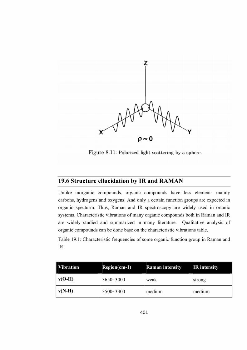
401

19.6 Structure ellucidation by IR and RAMAN

Unlike inorganic compounds, organic compounds have less elements mainly carbons, hydrogens and oxygens. And only a certain function groups are expected in organic specturm. Thus, Raman and IR spectroscopy are widely used in ortanic systems. Characteristic vibrations of many organic compounds both in Raman and IR are widely studied and summarized in many literature. Qualitative analysis of organic compounds can be done base on the characteristic vibrations table.

Table 19.1: Characteristic frequencies of some organic function group in Raman and IR

Vibration Region(cm-1) Raman intensity IR intensity

v(O-H) 3650~3000 weak strong

v(N-H) 3500~3300 medium medium

402

v(C=O) 1820~1680 strong~weak very strong

v(C=C) 1900~1500 Very strong~medium

0~weak

“RS is similar to IR in that they have regions that are useful for functional group detection and fingerprint regions that permit the identification of specific compounds.” While from the different selection rules of Raman Spectroscopy and IR, we can get the Mutual Exclusion rule, which says that for a molecule with a center of symmetry, no mode can be both IR and Raman Spectroscopy active. So, if we find a strong bond which is both IR and Raman Spectroscopy active, the molecule doesn't have a center of symmetry.

19.1 Choose the correct answer (After 19.6).

a) The selection rule of stock line in Rotational roman spectra of a moleaucule is –

1) ΔJ = --2 (ii) ΔJ = T2 (iii) ΔJ = o (iv) Δ J = PI

b) which of the molecuele is microwave active.

(i) HCL (ii) CO2 (iii) H2 (iv) O2

c) Roman effect is:--

(i) absortion of light (ii) emission of light (iii)in elastic scaltening of light (iv) eelastic

scattering.

d) which is ER in actime but Roman active.

(i) HCL (ii) SO2 (iii) N2 (iv) Protein

19.2 Complete the following :--

a) Depalarization ratio e=…………………

b) IR forbidden normal modes are Roman ------------------

403

c) Assgmmatrical stretching is IR -----------------------.

d) Stokes lines are more intense than -------------- lines

19.7 Applications

Raman Spectroscopy(RS) application in inorganic systems

X-ray diffraction (XRD) has been developed into a standard method of determining structure of solids in inorganic systems. Compared to XRD, it is usually necessary to obtain other information (NMR, electron diffraction, or UV-Visible) besides vibrational information from IR/Raman in order to elucidate the structure. Nevertheless, vibrational spectroscopy still plays an important role in inorganic systems. For example, some small reactive molecules only exist in gas phase and XRD can only be applied for solid state. Also, XRD cannot distinguish between the following bonds: –CN vs. –NC, –OCN vs. –NCO,–CNO vs. –ONC, -SCN vs. –NCS. Furthermore, IR and Raman are fast and simple analytical method, and are commonly used for the first approximation analysis of an unknown compound.

Raman spectroscopy has considerable advantages over IR in inorganic systems due to two reasons. First, since the laser beam used in RS and the Raman-scattered light are both in the visible region, glass (Pyrex) tubes can be used in RS. On the other hand, glass absorbs infrared radiation and cannot be used in IR. However, some glass tubes, which contain rare earth salts, will gives rises to fluorescence or spikes. Thus, using of glass tubes in RS still need to be careful. Secondly, since water is a very weak Raman scatter but has a very broad signal in IR, aqueous solution can be directly analyzed using RS.

Raman Spectroscopy and IR have different selection rules. RS detects the polarizability change of a molecule, while IR detects the dipole momentum change of a molecule. Thus, some vibration modes that are active in Raman may not be active IR, vice versa. As a result, both of Raman and IR spectrum are provided in the stucture study. As an example, in the study of Xenon Tetrafluoride. There are 3 strong bands in IR and solid Raman shows 2 strong bands and 2 weaker bands. These information indicates that Xenon Tetrafluoride is a planar molecule and has a symmetry of D4h. Another example is the application of Raman Spectroscopy in homonuclear diatomic molecules. Homonuclear diatomic molecules are all IR inactive, fortunately, the vibration modes for all the homonuclear diatomic molecules

404

are always Raman Spectroscopy active.

Raman Spectroscopy Application in Organic Systems

Unlike inorganic compounds, organic compounds have less elements mainly carbons, hydrogens and oxygens. And only a certain function groups are expected in organic specturm. Thus, Raman and IR spectroscopy are widely used in organic systems. Characteristic vibrations of many organic compounds both in Raman and IR are widely studied and summarized in many literature (Table 19.2)

Table 19.2

RS is similar to IR in that they have regions that are useful for functional group detection and fingerprint regions that permit the identification of specific compounds.” While from the different selection rules of Raman Spectroscopy and IR, we can get the Mutual Exclusion rule, which says that for a molecule with a center of symmetry, no mode can be both IR and Raman Spectroscopy active. So, if we find a strong bond which is both IR and Raman Spectroscopy active, the molecule doesn't have a center of symmetry.

Application of Infrared spectra(IR)

Since different molecules with different combination of atoms produce their unique spectra, infrared spectroscopy can be used to qualitatively identify substances. In addition, the intensity of the peaks in the spectrum is proportional to the amount of substance present, enabling its application for quantitative analysis.

Qualitative analysis

For qualitative identification purposes, the spectrum is commonly presented as transmittance versus wavenumber. Functional groups have their characteristic fundamental vibrations which give rise to absorption at certain frequency range in the Each band in a spectrum can be attributed to stretching or bending mode of a bond.

Almost all the fundamental vibrations appear in the mid-infrared region. For

405

instance, 4000 – 2500 cm-1 region usually can be assigned to stretching modes of O-H, N-H or C-H. Triple-bond stretching modes appear in the region of 2500 – 2000 cm-1. C=C and C=O stretching bands fall in the 2000 – 1500 cm-1 region. Hence, characterization of functional groups in substances according to the frequencies and intensities of absorption peaks is feasible, and also structures of molecules can be proposed. This method is applicable to organic molecules, inorganic molecules, polymers, etc. A detailed frequency list of functional groups. Note that several functional groups may absorb at the same frequency range, and a functional group may have multiple-characteristic absorption peaks, especially for 1500 – 650 cm-1, which is called the fingerprint region.

Bands in the near-infrared region are overtones or combination bands. They are weak in intensity and overlapped, making them not as useful for qualitative analysis as those in mid-infrared region. However, absorptions in this region are helpful in exploiting information related to vibrations of molecules containing heavy atoms, molecular skeleton vibrations, molecular torsions and crystal lattice vibrations.

Quantitative analysis

Absorbance is used for quantitative analysis due to its linear dependence on concentration. Given by Beer-Lambert law, absorbance is directly proportional to the concentration and pathlength of sample:

A= εcl …………19.14

where A is absorbance, ε the molar extinction coefficient or molar absorptivity which is characteristic for a specific substance, c the concentration and l the pathlength (or the thickness) of sample. The conversion from transmittance to absorbance is given by

A=−logT …………19.15

where T is transmittance.

For quantitative analysis of liquid samples, usually an isolated peak with high molar absorptivity that appears in the spectrum of the compound is chosen. A calibration curve of absorbance at the chosen frequency against concentration of the compound is acquired by measuring the absorbance of a series of standard compound solution with known concentrations. These data are then graphed to get a linear plot, from which the concentration of the unknown can be calculated after measuring its

406

absorbance at the same frequency. The number of functional groups can also be calculated in this way, since the molar absorptivity of the band is proportional to the number of functional groups that are present in the compound.

For solid samples, an internal standard with a constant known amount is added to the unknown sample and the standards. Then similar procedures as those with liquid samples are carried out except that the calibration curve is a graph of the ratio of absorbance of analyte to that of the internal standard versus concentration of the analyte.

A multi-component analysis of the mixture is also feasible since different components have different values of molar absorptivity at the same frequency.

19.8 Summary

Raman spectroscopy in value study of vileratand rotational energy changes by seattaining of light.

Raman scattering show certain discrete peg, uencies above ad below that of incident beam.

Intenlity of Raman live depend on concentortion of the surbrtanc.

For Raman effect molecure must show a change in palarisalisty along internucularo akis in palarisality


19.1 (a) (ii), (b) (ii), (C) (iii), d (iii)

19.2 (a I1/III (b) allowed (c) acuter (d) Antismoke

19.10 References and suggested Readings

Sources

1. http://en.wikipedia.org/wiki/Raman_spectroscopy 2. http://astro1.panet.utoledo.edu/~relling2/teach/4780/20101101_lecture_10_phys4

780.pdfastro1.panet.utoledo.edu

407

3. http://www.colorado.edu/chemistry/volkamer/teaching/RefMaterial/Bernath_2005_ch8.pdf

4. http://chemwiki.ucdavis.edu/Physical_Chemistry/Spectroscopy/Vibrational_Spectroscopy/Infrared_Spectroscopy/Infrared%3A_Application

408

Unit -20 : Electronic spectroscopy of molecules

Structure of Unit

20.0 Objectives

20.1 Introduction

20.2 Born–Oppenheimer approximation

20.3 Electronic Spectra of Diatomic Molecules

20.4 Vibrational coarse structure

20.5 Rotational fine structure of electronic – vibration spectrum

20.6 Photoelectron Spectroscopy

20.7 Electron spin resonance

20.8 Mössbauer spectroscopy

20.9 Summary

20.10 Glassory

Answer to key assessment Questions



20.0 Objectives


Basic principles of Electronic spectroscopy.

Born-oppenhmier approximation.

Electronic spectra of diatomic molecules.

Vibrational coarse structure and rotational fine structure?

What is photo electron spectroscopy and what are its applications?

What is electron spin resonance spectroscopy and what are its applications?

409

What is mossbaure spectroscopy and what are its application?

20.1 Introduction

Electronic Spectroscopy relies on the quantized nature of energy states. Given enough energy, an electron can be excited from its initial ground state or initial excited state (hot band) and briefly exist in a higher energy excited state. Electronic transitions involve exciting an electron from one principle quantum state to another. Without incentive, an electron will not transition to a higher level. Only by absorbing energy, can an electron be excited. Once it is in the excited state, it will relax back to it's original more energetically stable state, and in the process, release energy as photons.

Electron spectroscopy is an analytical technique to study the electronic structure and its dynamics in atoms and molecules. In general an excitation source such as x-rays, electrons or synchrotron radiation will eject an electron from an inner-shell orbital of an atom. Detecting photoelectrons that are ejected by x-rays is called x-ray photoelectron spectroscopy (XPS) or electron spectroscopy for chemical analysis (ESCA). Detecting electrons that are ejected from higher orbitals to conserve energy during electron transitions is called Auger electron spectroscopy (AES).

During electronic spectroscopy, the electron is excited first from an initial low energy state to a higher state by absorbing photon energy from the spectrophotometer. If the wavelength of the incident beam has enough energy to promote an electron to a higher level, then we can detect this in the absorbance spectrum. Once in the excited state, the electron has higher potential energy and will relax back to a lower state by emitting photon energy. This is called fluorescence and can be detected in the spectrum as well. Embedded into the electronic states (n=1,2,3...) are vibrational levels (v=1,2,3...) and within these are rotational energy levels (j=1,2,3...).

Often, during electronic transitions, the initial state may have the electron in a level that is excited for both vibration and rotation. In other words, n=0, v does not = 0 and r does not =0. This can be true for the ground state and the excited state. (Fig 20.1) In addition, due to the Frank Condon Factor, which describes the overlap between vibrational states of two electronic states, there may be visible vibrational bands within the absorption bands. Therefore, vibrational fine structure that can be seen in the absorption spectrum gives some indication of the degree of Frank Condon overlap between electronic states.

410

Fig. 20.1 Transtions from different states

The Selection Rules governing transitions between electronic energy levels of transition metal complexes are:

ΔS = 0 The Spin Rule ……………(20.1)

Δl = +/- 1 The Orbital Rule (Laporte) ……………(20.2)

The first rule says that allowed transitions must involve the promotion of electrons without a change in their spin.

The second rule says that if the molecule has a centre of symmetry, transitions within a given set of p or d orbitals (i.e. those which only involve a redistribution of electrons within a given subshell) are forbidden.

Relaxation of the Rules can occur through

a) Spin-Orbit coupling - this gives rise to weak spin forbidden bands

b) Vibronic coupling - an octahedral complex may have allowed vibrations where the molecule is asymmetric.

Absorption of light at that moment is then possible.

c) π-acceptor and π-donor ligands can mix with the d-orbitals so transitions are no longer purely d-d.

Types of transition

Charge transition, either ligand to metal or metal to ligand. These are often extremely intense and are generally found in the UV but they may have a tail into the visible.

d-d, these can occur in both the UV and visible region but since they are forbidden transitions they have small intensities.

411

20.2 Born–Oppenheimer approximation

In quantum chemistry, the computation of the energy and the wavefunction of an average-size molecule is a formidable task that is alleviated by the Born–Oppenheimer (BO) approximation, named after Max Born and J. Robert Oppenheimer. For instance the benzene molecule consists of 12 nuclei and 42 electrons. The time independent Schrödinger equation, which must be solved to obtain the energy and wavefunction of this molecule, is a partial differential eigenvalue equation in 162 variables—the spatial coordinates of the electrons and the nuclei. The BO approximation makes it possible to compute the wavefunction in two less complicated consecutive steps. This approximation was proposed in 1927, in the early period of quantum mechanics, by Born and Oppenheimer and is still indispensable in quantum chemistry.

In basic terms, it allows the wavefunction of a molecule to be broken into its electronic and nuclear (vibrational, rotational) components.

Ψmolecule = Ψelectron x Ψnuclei ……………(20.3)

In molecular spectroscopy, because the ratios of the periods of the electronic, vibrational and rotational energies are each related to each other on scales in the order of a thousand, the Born–Oppenheimer name has also been attached to the approximation where the energy components are treated separately.

Etotal = Eelectronic + Evibrational + Erotational + Enuclear ……………(20.4)

The nuclear spin energy is so small that it is normally omitted.

The Born-Oppenheimer approximation is one of the basic concepts underlying the description of the quantum states of molecules. This approximation makes it possible to separate the motion of the nuclei and the motion of the electrons. This is not a new idea for us. We already made use of this approximation in the particle-in-a-box model when we explained the electronic absorption spectra of cyanine dyes without considering the motion of the nuclei. Then we discussed the translational, rotational and vibrational motion of the nuclei without including the motion of the electrons. In this chapter we will examine more closely the significance and consequences of this important approximation. Note, in this discussion nuclear refers to the atomic nuclei as parts of molecules not to the internal structure of the nucleus.

The Born-Oppenheimer approximation neglects the motion of the atomic nuclei

412

when describing the electrons in a molecule.

The physical basis for the Born-Oppenheimer approximation is the fact that the mass of an atomic nucleus in a molecule is much larger than the mass of an electron (more than 1000 times). Because of this difference, the nuclei move much more slowly than the electrons. In addition, due to their opposite charges, there is a mutual attractive

force of 2

2

Zer

acting on an atomic nucleus and an electron. This force causes both

particles to be accelerated. Since the magnitude of the acceleration is inversely proportional to the mass, a = f/m, the acceleration of the electrons is large and the acceleration of the atomic nuclei is small; the difference is a factor of more than 1000. Consequently, the electrons are moving and responding to forces very quickly, and the nuclei are not. You can imagine running a 100-yard dash against someone whose acceleration is a 1000 times greater than yours. That person could literally run circles around you. So a good approximation is to describe the electronic states of a molecule by thinking that the nuclei aren't moving, i.e. that they are stationary. The nuclei, however, can be stationary at different positions so the electronic wavefunction can depend on the positions of the nuclei even though their motion is neglected.

20.3 Electronic Spectra of Diatomic Molecules

Transition between electronic energy levels of molecules leads to emission or absorption in visible and U.V region . Some times the energy change of transition of some molecule is so high that the spectrum appear at Vacuum UV . All molecules can give electronic spectra.

Using Born – Oppenhiemer approximation-

Etot = Eelec. + Evib + Erot

ΔƐtot = ΔƐelec. + ΔƐvib + ΔƐrot

The approximate order of magnitude of these changes are

ΔƐelec.≈ 103 x ΔƐvib ≈ 106 x ΔƐrot …….(20.5)

Vibrational change will produce " coarse structure " and rotational change produce

"fine structure " Ignoring Ɛrot "

ΔƐtot = ΔƐelec. + ΔƐvib …….(20.6)

413

…….(20.7)

Electronic spectra arise from transitions in which the electronic state of the molecule changes - these are the transitions most nearly analogous to atomic transitions, and typically involve photons in the visible and ultraviolet parts of the spectrum. At low resolution, electronic spectra seem to be made up of series of more or less evenly space bands; at higher resolution, each band is made of many individual spectral lines.

To understand these spectra, recall that we have found that the energy of a single level of electronic state s, vibrational state v, and rotational level J may be written as a sum of these three energies, Et = Es + Ev + Ej, so that the frequency of a particular transition will be given by

G(j' j") = V(v' - v") + B' j' (j' + 1) - B" j"(j" + 1) …….(20.8)

Here B are rotational constants and J are rotational quantum numbers. (For B also, a double prime indicates the ground state and a single prime an electronically excited state.) The values of the rotational constants may differ appreciably because the bond length in the electronic excited state may be quite different from the bond length in the ground state, because of the operation of the Franck-Condon principle. The rotational constant is inversely proportional to the square of the bond length. Usually

B′< B′′ as is true when an electron is promoted from a bonding orbital to an antibonding orbital, causing bond lengthening. But this is not always the case; if an electron is promoted from a non-bonding or antibonding orbital to a bonding orbital,

there will be bond-shortening and B′> B′′. Selection rules control which electronic states can make strong transitions with each other; these are somewhat complicated and will not be treated here. There is no selection rule on the difference v = v' - v", since the two vibrational levels are not formed in the same electronic potential well, and values of Delta v up to 5 or 6 are not uncommon. Since the rotational energies involve the same angular functions in both states, they continue to observe the selection rule J = +/- 1 between two Sigma states, or J = 0, +/-1 for states with Lambda not equal 0.

20.4 Vibrational coarse structure

To understand the vibrational coarse structure, we drop the rotational energy term

414

from the expression for total energy

…..(20.9)

For v = 0,1,2,3,4… …………The energy levels corresponding to this equation are shown in the following figure. (20.2)

The lower states are indicated by a (") and the upper by (')

The vibrational levels in the excited state would be more closely spaced that in the ground state. From the above equation the frequency of a spectral line can be written as

…..(20.10)

Fig. 20.2 Vibrational coarse structure of electronic absorption from ground

state

Any transition (v" - v') has some definite probability . However the situation is simple if the absorption is from the electronic ground state to an excited state, as almost all molecules exist in the lowest vibrational state. Therefore the transitions which are of considerable intensity are those originating from the v"=0 state , labeled

415

according to their (v" - v') values as (0,0), (1,0), (2,0), (3,0).The set of lines corresponding to these transition is called a v' progression since the value of v' increases by unity for each line in the site .

The wave number of the (0,0) transition is then.

…..(20.11)

From the above equation, one can be determined the vibrational frequency(we) and an harmonicity constant(Xe) of both ground and excited electronic states of a molecule in addition to separation between the electronic state .

20.5 Rotational fine structure of electronic – vibration spectrum

We Know that…

…..(20.12)

Et is the total energy, while Eel. and Ev are the electronic and vibrational energies. selection rule for j = +/- 1

…..(20.13)

Et is the total energy, while Eel. and Ev are the electronic and vibrational energies. selection rule for j = +/- 1

Then the frequencies of the transition are

………..(20.14)

Replacing the first two terms by the wave number of an electronic vibrational transition

…………..(20.15)

could by any one of the (0,0), (1,0) ,(2,0)

The selection rule for J depends on the type of electronic transition. Transition for

416

which both the upper and lower states have no electronic angular momentum about

the inter nuclear axis the selection rule is ΔJ= +1

This lead to the presence of both P and R branches for all transitions

…………..(20.19)

with the restriction that a state with J=0 cannot undergo a transition J=0 state . That is

J=0 ----> J=0 in such cases Q branch will also be there in addition to p and R branches. We shall now consider the rotational contribution in equation detail for P branch DJ=-1 or J '- J" = -1.

The rotational contribution

…………..(20.17)

As the lowest value of J' =1 for P branch , there will not be any spectral line at for R branch , J' - J" = +1

…………..(20.18)

for Q branch

…..(20.19)

J" cannot be zero as that would mean a transition from J=0 state to another J=0. There will be no spectral line at in the red Q branches.

20.6 Photoelectron Spectroscopy

Photoelectron spectroscopy (PES) is a technique used for determining the ionization potentials of molecules. Underneath the banner of PES are two separate techniques

417

for quantitative and qualitative measurements. They are ultraviolet photoeclectron spectroscopy (UPS) and X-ray photoelectron spectroscopy (XPS). XPS is also known under its former name of electron spectroscopy for chemical analysis (ESCA). UPS focuses on inoization of valence electrons while XPS is able to go a step further and ionize core electrons.

Prior to 1960, virtually all measurements of photoelectron kinetic energies were for electrons emitted from metals and other solid surfaces. About 1956 Kai Siegbahn developed X-ray photoelectron spectroscopy (XPS) for surface chemical analysis. This method uses x-ray sources to study energy levels of atomic core electrons, and at the time had an energy resolution of about 1 eV (electronvolt).

The ultraviolet method (UPS) was developed to study the photoelectron spectra of free molecules in the gas phase by David W. Turner, a physical chemist at Imperial College in London and then at Oxford University, in a series of publications from 1962 to 1967. As a photon source, he used a helium discharge lamp which emits a wavelength of 58.4 nm (corresponding to an energy of 21.2 eV) in the vacuum ultraviolet region. With this source Turner’s group obtained an energy resolution of 0.02 eV. Turner referred to the method as “molecular photoelectron spectroscopy”, now usually “Ultraviolet photoelectron spectroscopy” or UPS. As compared to XPS, UPS is limited to energy levels of valence electrons, but measures them more accurately. After 1967 commercial UPS spectrometers became available.

If Einstein’s photoelectric law is applied to a free molecule, the kinetic energy ( Ek) of an emitted photoelectron is given by

Ek = h - I …………..(20.20)

where h is Planck’s constant, ν is the frequency of the ionizing light, and I is an ionization energy for the formation of a singly charged ion in either the ground state or an excited state. According to Koopmans' theorem, each such ionization energy may be identified with the energy of an occupied molecular orbital. The ground-state ion is formed by removal of an electron from the highest occupied molecular orbital, while excited ions are formed by removal of an electron from a lower occupied orbital.

(A) Photoelectron Instrumentation

The main goal in either UPS or XPS is to gain information about the composition, electronic state, chemical state, binding energy, and more of the surface region of

418

solids. The key point in PES is that a lot of qualitative and quantitative information can be learned about the surface region of solids. Specifics about what can be studied using XPS or UPS will be discussed in detail below in separate sections for each technique following a discussion on instrumentation for PES experiments. The focus here will be on how the instrumentation for PES is constructed and what types of systems are studied using XPS and UPS. The goal is to understand how to go about constructing or diagramming a PES instrument, how to choose an appropriate analyzer for a given system, and when to use either XPS or UPS to study a system.

There are a few basics common to both techniques that must always be present in the instrumental setup.

(B) A radiation source: The radiation sources used in PES are fixed-energy radiation sources. XPS sources from x-rays while UPS sources from a gas discharge lamp. An analyzer: PES analyzers are various types of electron energy analyzers A high vacuum environment: PES is rather picky when it comes to keeping the surface of the sample clean and keeping the rest of the environment free of interferences from things like gas molecules. The high vacuum is almost always an ultra high vacuum (UHV) environment.

Radiation sources

While many components of instruments used in PES are common to both UPS and XPS, the radiation sources are one area of distinct differentiation. The radiation source for UPS is a gas discharge lamp, with the typical one being an He discharge lamp operating at 58.4 nm which corresponds to 21.2 eV of kinetic energy. XPS has a choice between a monocrhomatic beam of a few microns or an unfocused non-monochromatic beam of a couple centimeters. These beams originate from X-Ray sources of either Mg or Al K-? sources giving off 1486 eV and 1258 eV of kinetic energy respectively. For a more versitile light source, synchrotron radiation sources are also used. Synchrotron radiation is especially useful in studying valence levels as it provides continuous, polarized radiation with high energies of > 350 eV.

The main thing to consider when choosing a radiation source is the kinetic energy involved. The source is what sets the kinetic energy of the photoelectrons, so there needs to not only be enough energy present to cause the ionizations, but there must also be an analyzer capable of measuring the kinetic energy of the released photoelectrons.

419

(C) Analyzers

There are two main classes of analyzers well-suited for PES - kinetic energy analyzers and deflection or electrostatic analyzers. Kinetic energy analyzers have a

resolving power of E/δE, which means the higher the kinetic energy of the photoelectrons, the lower the resolution of the spectra. Deflection analyzers are able to separate out photoelectrons through an electric field by forcing electrons to follow

different paths according to their velocities, giving a resolving power, E/δE, that is greater than 1,000.

Since the resolving power of both types of analyzer is E/δE, the resolution is directly dependent on the kinetic energy of the photoelectrons. The intensity of the spectra produced is also dependent on the kinetic energy. The faster the electrons are moving, the lower the resolution and intensity is. In order to actually get well resolved, useful data other components must be introduced into the instrument.

In XPS experiments, electron guns can also be used in conjunction with x-rays to eject photoelectrons. There are a couple of advantages and disadvantages to doing this, however. With an electron gun, the electron beam is easily focused and the excitation of photoelectrons can be constantly varied. Unfortunately, the background radiation is increased significantly due to the scattering of falling electrons. Also, a good portion of substances that are of any experimental interest are actually decomposed by heavy electron bombardment such as that coming from an electron gun.

(D) Detection & Spectra

Detection relies on the ability of the instrument to measure energy and photoelectron output. One type of energy measured is the binding energy, which is calculated through the following equation:

Ke = hν−BE−ϕ ……(20.21)

where:

Ke= Kinetic energy, this is measured

hν = Photon energy from the radiation source, this is controlled by the source

ϕ= Work function of the spectrometer, this is found through calibration

BE= Binding energy, this is the unknown of interest and can be calculated from the

420

other three variables

Another part of PES detection is in the use of electron multipliers. These devices act as electron amplifiers because they are coated with a material that produce secondary photoelectrons when they are struck by an electron. Typically, they are able to produce two to three photoelectrons per every electron they are hit with. Since the signals in PES are low, the huge amplification, up to 107 and higher when run in series so the secondary electrons from one multiplier strike the next, they greately improve the signal strength from these instruments.

20.7 Electron spin resonance

Electron paramagnetic resonance spectroscopy (EPR), also called electron spin resonance (ESR), is a technique used to study chemical species with unpaired electrons. EPR spectroscopy plays an important role in the understanding of organic and inorganic radicals, transition metal complexes, and some biomolecules.

Like most spectroscopic techniques, EPR spectrometers measure the absorption of electromagnetic radiation. However, a phase-sensitive detector is used in EPR spectrometers which converts the normal absorption signal to its first derivative. Then the absorption signal is presented as its first derivative in the spectrum, which is similar to the one on the bottom of Figure (Fig 20.3). Thus, the magnetic field is on

the x-axis of EPR spectrum; dχ″/dB, the derivative of the imaginary part of the molecular magnetic susceptibility with respect to the external static magnetic field in arbitrary units is on the y-axis. In the EPR spectrum, where the spectrum passes through zero corresponds to the absorption peak of absorption spectrum. People can use this to determine the center of the signal. On the x-axis, sometimes people use the unit “gauss” (G), instead of tesla (T). One tesla is equal to 10000 gauss.

Electron spin resonance is a magnetic resonance technique, based on the interaction of unpaired electron spins with an external magnetic field. The essential aspects of ESR may be illustrated by considering the hypothetical case of a single isolated electron. This electron is characterized by the quantum number S = 1/2 and possesses a magnetic moment:

……(20.22)

withge=2.0023, the electron g-factor or Landé-factor,Be=9.42 . 10–24 J.T–1, the electronic Bohr magneton and Sr, the dimensionless electron spin vector. In a

421

magnetic field, B0, there are two energy states for this electron. This interaction, known as the Zeeman interaction, is expressed by the following Hamiltonian:

……(20.23)

Fig. 20.3 Abrorytion Signal

Two energy levels evolve, viz. Eb=–1/2 ge .be . B0 and Ea=+1/2ge .be .B0, which are almost equally populated. In ESR spectroscopy, the magnetic component of a microwave energy, which is perpendicular to the magnetic field B0, induces microwave energy absorption subject to the resonance condition and the selection rule delta Ms = ±1:

……(20.24)

wheren is the microwave frequency.

In real chemical systems, the single unpaired electron is associated with at least one atom and the second contribution to paramagnetism stems from the electron motion in an orbital with orbital angular momentum L. This effect can be described by the following Hamiltonian:

……(20.25)

withl, the spin-orbit coupling constant and g, the effective g-value. The orbitals (atomic or molecular) have two effects: (1) spin-orbit coupling and (2) orbitalmagnetic field interaction. These effects explain why g is no longer equal to

422

2.0023 (=ge) and anisotropic. The anisotropy of the g"-tensor leads to orientationdependent ESR-spectra for single crystals, but for disordered systems as in the case of molecular sieves, one observes the superposition of spectra of all possible orientations of the magnetic field. Idealized ESR patterns, together with their corresponding absorption profile. The anisotropy in g is classified into isotropic (one g-value), axial (two g-values) and rhombic (three g-values). The deviation of the principal g-values from the free electron value of 2.0023 carries information about the orbital angular momentum of the electron, i.e. information concerning the electronic structure of the atom or molecules.

Applications

EPR/ESR spectroscopy is used in various branches of science, such as biology, chemistry and physics, for the detection and identification of free radicals and paramagnetic centers such as F centers. EPR is a sensitive, specific method for studying both radicals formed in chemical reactions and the reactions themselves. For example, when ice (solid H2O) is decomposed by exposure to high-energy radiation, radicals such as H, OH, and HO2 are produced. Such radicals can be identified and studied by EPR. Organic and inorganic radicals can be detected in electrochemical systems and in materials exposed to UV light. In many cases, the reactions to make the radicals and the subsequent reactions of the radicals are of interest, while in other cases EPR is used to provide information on a radical's geometry and the orbital of the unpaired electron.

Transition Metal Ions

Transition metal ions (TMIs) coordinate to lattice oxygen atoms, form complexes inside the cages and/or channels or occupy framework sites. Classical ESR techniques as well as pulsed ESR, and in particular the analysis of the modulation of the echo envelope signal (ESEEM) has been used extensively to gather detailed information about the coordination environment of TMIs.

20.8 Mössbauer spectroscopy

(A) Introduction

Mössbauer spectroscopy is a spectroscopic technique based on the Mössbauer effect. This effect, discovered by Rudolf Mössbauer in 1957, consists of the recoil-free, resonant absorption and emission of gamma rays in solids.

423

Like NMR spectroscopy, Mössbauer spectroscopy probes tiny changes in the energy levels of an atomic nucleus in response to its environment. Typically, three types of nuclear interactions may be observed: an isomer shift, also known as a chemical shift; quadrupole splitting; and magnetic or hyperfine splitting, also known as the Zeeman effect. Due to the high energy and extremely narrow line widths of gamma rays, Mössbauer spectroscopy is a very sensitive technique in terms of energy (and hence frequency) resolution, capable of detecting change in just a few parts per 1011.

Mössbauer spectroscopy is a versatile technique used to study nuclear structure with the absorption and re-emission of gamma rays, part of the electromagnetic spectrum. The technique uses a combination of the Mössbauer effect and Doppler shifts to probe the hyperfine transitions between the excited and ground states of the nucleus. (Fig. 20.4) Mössbauer spectroscopy requires the use of solids or crystals which have a probability to absorb the photon in a recoilless manner, many isotopes exhibit Mössbauer characteristics but the most commonly studied isotope is 57Fe.

Rudolf L. Mössbauer became a physics student at Technical University in Munich at the age of 20. After passing his intermediate exams Mössbauer began working on his thesis and doctorate work in 1955, while working as an assistant lecturer at Institute for Mathematics.In 1958 at the age of 28 Mössbauer graduated, and also showed experimental evidence for recoilless resonant absorption in the nucleus, later to be called the Mössbauer Effect.In 1961 Mössbauer was awarded the Nobel Prize in physics and, under the urging of Richard Feynman, accepted the position of Professor of Physics at the California Institute of Technology.

Fig. 20.4 Ground and Excited states

(B) Mössbauer Effect

The recoil energy associated with absorption or emission of a photon can be described by the conservation of momentum.In it we find that the recoil energy

424

depends inversely on the mass of the system. For a gas the mass of the single nucleus is small compared to a solid.The solid or crystal absorbs the energy as phonons, quantized vibration states of the solid, but there is a probability that no phonons are created and the whole lattice acts as the mass, resulting in a recoilles emission of the gamma ray. The new radiation is at the proper energy to excite the next ground state nucleus. The probability of recoilles events increases with decreasing transition energy.

Just as a gun recoils when a bullet is fired, conservation of momentum requires a free nucleus (such as in a gas) to recoil during emission or absorption of a gamma ray. If a nucleus at rest emits a gamma ray, the energy of the gamma ray is slightly less than the natural energy of the transition, but in order for a nucleus at rest to absorb a gamma ray, the gamma ray's energy must be slightly greater than the natural energy, because in both cases energy is lost to recoil. This means that nuclear resonance (emission and absorption of the same gamma ray by identical nuclei) is unobservable with free nuclei, because the shift in energy is too great and the emission and absorption spectra have no significant overlap.

Nuclei in a solid crystal, however, are not free to recoil because they are bound in place in the crystal lattice. When a nucleus in a solid emits or absorbs a gamma ray, some energy can still be lost as recoil energy, but in this case it always occurs in discrete packets called phonons (quantized vibrations of the crystal lattice). Any whole number of phonons can be emitted, including zero, which is known as a "recoil-free" event. In this case conservation of momentum is satisfied by the momentum of the crystal as a whole, so practically no energy is lost.

As an analogy, imagine jumping from a boat to shore, and imagine that the distance from the boat to shore is the longest you can possibly jump (on land). If the boat is floating in water, you will fall short because some of your energy goes into pushing the boat back. If the water is frozen solid, however, you will be able to make it.

Mössbauer found that a significant fraction of emission and absorption events will be recoil-free, which is quantified using the Lamb–Mössbauer factor. This fact is what makes Mössbauer spectroscopy possible, because it means gamma rays emitted by one nucleus can be resonantly absorbed by a sample containing nuclei of the same isotope, and this absorption can be measured.

(d) Mössbauer Isotopes

425

By far the most common isotopes studied using Mössbauer spectroscopy is 57Fe, but many other isotopes have also displayed a Mössbauer spectrum.

The excited state is of very low energy, resulting in a small change in energy between ground and excited state. This is because gamma rays at higher energy are not absorbed in a recoil free manner, meaning resonance only occurs for gamma rays of low energy.

The resolution of Mössbauer spectroscopy depends upon the lifetime of the excited state. The longer the excited state lasts the better the image.

Both conditions are met by 57Fe and it is thus used extensively in Mössbauer spectroscopy. In the figure to the right the red colored boxes of the periodic table of elements indicate all elements (Fig. 20.5) that have isotopes visible using the Mössbauer technique.

Fig. 20.5 Periodie table

(g) Applications

Among the drawbacks of the technique are the limited number of gamma ray sources and the requirement that samples be solid in order to eliminate the recoil of the nucleus. Mössbauer spectroscopy is unique in its sensitivity to subtle changes in the chemical environment of the nucleus including oxidation state changes, the effect of different ligands on a particular atom, and the magnetic environment of the sample.

As an analytical tool Mössbauer spectroscopy has been especially useful in the field of geology for identifying the composition of iron-containing specimens including meteors and moon rocks. In situ data collection of Mössbauer spectra has also been

426

carried out on iron rich rocks on Mars.

Another significant application of Mössbauer spectroscopy is the study of phase transformations that occur in iron catalysts during Fischer–Tropsch synthesis. While these catalysts initially consist of hematite (Fe2O3), during reaction they are transformed into a mixture of magnetite (Fe3O4) and several iron carbides. The formation of carbides appears to improve catalytic activity, however it can also lead to the mechanical break-up and attrition of the catalyst particles. This can cause difficulties in the final separation of catalyst from reaction products.

Mössbauer spectroscopy has also been used to determine the relative concentration change in the oxidation state of antimony (Sb) during the selective oxidation of olefins. During calcination all the Sb ions in an antimony-containing tin dioxide catalyst transform into the +5 oxidation state. Following the catalytic reaction, almost all Sb ions revert from the +5 to the +3 oxidation state. A significant change in the chemical environment surrounding the antimony nucleus occurs during the oxidation state change which can easily be monitored as an isomer shift in the Mössbauer spectrum.

This technique has also been used to observe the second-order transverse Doppler effect predicted by the theory of relativity, because of very high energy resolution.

20.1 Choose the correct alternative

a) The energy required for various transitions fallow the order.

(i) _ → ҇ * > n→>π→π n →π *

(ii) n→π*>n→҇*>π—π>-- -- *

(iii) both (iv) none.

b) An an chrome is one which is

(i)colour enhancing (ii) extended conjugation (iii) a group with lane pain of election

(iv) all

c) ultar violent spectra scopy for detation of –

427

(i) functionat group (ii) extent of configuration (iii) geometrical issomass(iv) all

d) Mosshaver spectroscopy deals with mass haver effect and---

(i) Doppler shift (ii) dipole moment (iii) both (iv) None.

e) EPR is also called as :--

(i) NMR (ii) ESR (iii) UV (iv) all.

f) 1 tesla is equal to how maney gauss:--

(i) 10 (ii)1000 (iii) 10000 (iv) all.

20.9 Summary

The above unit explains the Electron spectroscopy is an analytical technique to study the electronic structure and its dynamics in atoms and molecules. In general an excitation source such as x-rays, electrons or synchrotron radiation will eject an electron from an inner-shell orbital of an atom. Detecting photoelectrons that are ejected by x-rays is called x-ray photoelectron spectroscopy (XPS) or electron spectroscopy for chemical analysis (ESCA). Detecting electrons that are ejected from higher orbitals to conserve energy during electron transitions is called Auger electron spectroscopy (AES).

The Selection Rules governing transitions between electronic energy levels of transition metal complexes are:

ΔS = 0 The Spin Rule

Δl = +/- 1 The Orbital Rule (Laporte)

Relaxation of the Rules can occur through

a) Spin-Orbit coupling - this gives rise to weak spin forbidden bands

b) Vibronic coupling - an octahedral complex may have allowed vibrations where the molecule is asymmetric.

Absorption of light at that moment is then possible.

428

c) π-acceptor and π-donor ligands can mix with the d-orbitals so transitions are no longer purely d-d.

In molecular spectroscopy, because the ratios of the periods of the electronic, vibrational and rotational energies are each related to each other on scales in the order of a thousand, the Born–Oppenheimer name has also been attached to the approximation where the energy components are treated separately.

Etotal = Eelectronic + Evibrational + Erotational + Enuclear

The nuclear spin energy is so small that it is normally omitted.

Using Born – Oppenhiemer approximation-

Etot = Eelec. + Evib + Erot

ΔƐtot = ΔƐelec. + ΔƐvib + ΔƐrot

In rotational fine structure of electronic – vibration spectrum The selection rule for J depends on the type of electronic transition. Transition for which both the upper and lower states have no electronic angular momentum about the inter nuclear axis the

selection rule is ΔJ= +1

In Photoelectron spectroscopy (PES) it is a technique used for determining the ionization potentials of molecules. Underneath the banner of PES are two separate techniques for quantitative and qualitative measurements. They are ultraviolet photoeclectron spectroscopy (UPS) and X-ray photoelectron spectroscopy (XPS).

Like NMR spectroscopy, Mössbauer spectroscopy probes tiny changes in the energy levels of an atomic nucleus in response to its environment. Typically, three types of nuclear interactions may be observed: an isomer shift, also known as a chemical shift; quadrupole splitting; and magnetic or hyperfine splitting, also known as the Zeeman effect. Due to the high energy and extremely narrow line widths of gamma rays, Mössbauer spectroscopy is a very sensitive technique in terms of energy (and hence frequency) resolution, capable of detecting change in just a few parts per 1011.

20.9 Glossary

Eelctromegnatic spectroscopy :-- study of the electronic structure nd its

dynamics in atones and molecules.

429

Electrons paramagnetic resonance spectroscopy :-- study of the chemical

species with unpaired electrons to external magnetic field.Fundamental

ultimate’s:-- Quantum treatment to the first vibrational transition from

zeroth vibrational level to the first.

Overtone:-- multiple of fundamental frequency.

20.1 Answer to say assessment questions

(a) (i), (b) (iv), (C) (iv), (d) (i), (e) (ii), (f) (iii)


1. http://en.wikipedia.org/wiki/Born%E2%80%93Oppenheimer_approximation

2. http://chemwiki.ucdavis.edu/Physical_Chemistry/Spectroscopy/Electronic_Spectroscopy/Electronic_Spectroscopy%3A_Interpretation

3. http://wwwchem.uwimona.edu.jm/courses/selrules.html

4. http://www.univsul.org/Dosekan_Wanekan_D/Electronic%20spectroscopy%20of20molecules.pdf

5. http://www.uotechnology.edu.iq/appsciences/physics/lecture/physics/four_class/spectral%20analysis/5.pdf

6. http://chemwiki.ucdavis.edu/Physical_Chemistry/Spectroscopy/Photoelectron_Spectroscopy/Photoelectron_Spectroscopy%3A_Application

7. http://chemwiki.ucdavis.edu/Physical_Chemistry/Spectroscopy/M%C3%B6ssbauer_Spectroscopy

8. http://en.wikipedia.org/wiki/M%C3%B6ssbauer_spectroscopy

430

Unit-21 : NMR Spectroscopy Structure of unit

21.1 Objectives

21.2 Introduction

21.3 Principal

21.4 Chemical shift

21.5 Continuous Wave (CW) NMR Spectrometer

21.6 Application of NMR spectroscopy in structure determination

21.7 Summary

21.8 Glossary

Answer to Key assessment Questions


21.1 Objectives

NMR spectroscopy is one of the most important technique for the structure determination of the organic compounds. This chapter deals with the basic principal and application of nuclear magnetic resonance spectroscopy and hence can be very useful for an chemist.

21.2 Introduction

Nuclear magnetic resonance spectroscopy, most commonly known as NMR spectroscopy, is a research technique that exploits the magnetic properties of certain atomic nuclei. It determines the physical and chemical properties of atoms or the molecules in which they are contained. It relies on the phenomenon of nuclear magnetic resonance and can provide detailed information about the structure, dynamics, reaction state, and chemical environment of molecules. The intramolecular magnetic field around an atom in a molecule changes the resonance frequency, thus giving access to details of the electronic structure of a molecule.

431

Most frequently, NMR spectroscopy is used by chemists and biochemists to investigate the properties of organic molecules, although it is applicable to any kind of sample that contains nuclei possessing spin. Suitable samples range from small compounds analyzed with 1-dimensional proton or carbon-13 NMR spectroscopy to large proteins or nucleic acids using 3 or 4-dimensional techniques. The impact of NMR spectroscopy on the sciences has been substantial because of the range of information and the diversity of samples, including solutions and solids.

NMR spectra are highly unique, well-resolved, analytically tractable and often highly predictable for small molecules. Thus, in organic chemistry practice, NMR analysis is used to confirm the identity of a substance. Different functional groups are obviously distinguishable, and identical functional groups with differing neighboring substituents still give distinguishable signals. The timescale of NMR is relatively long, and thus it is not suitable for observing fast phenomena, producing only an averaged spectrum. Although large amounts of impurities do show on an NMR spectrum, better methods exist for detecting impurities, as NMR is inherently not very sensitive.

NMR spectrometers are relatively expensive; universities usually have them, but they are less common in private companies. Modern NMR spectrometers have a very strong, large and expensive liquid helium-cooled superconducting magnet, because resolution directly depends on magnetic field strength. Less expensive machines using permanent magnets and lower resolution are also available, which still give sufficient performance for certain application such as reaction monitoring and quick checking of samples. There are even benchtop NMR spectrometers.

21.3 Principle of NMR spectroscopy

Nuclear magnetic resonance spectroscopy (NMR) has risen to the same level of importance as electronic and vibrational spectroscopy as a tool for studying molecular properties, particularly structural properties. Although the following discussion of nmr specifically deals with hydrogen atom nuclei in organic molecules, the principles described here apply to other types of molecules as well. Many other types of nuclei (13C, 19F, 31P, etc.) have nuclear spins and thus can be studied using NMR techniques.

Certain nuclei, such as the hydrogen nucleus (but not carbon-12 or oxygen-16), have

a nuclear spin. The spinning nucleus generates a small magnetic field, called "".

432

When placed in a strong external magnetic field, called Ho, the nucleus can exist in

two distinct spin states: a low energy state A, in which is aligned with the external

magnetic field, Ho, and a high energy state B, in which is opposed to the external

magnetic field, Ho. Alignment of with Ho is the more stable and lower energy state. (Fig. 21.1)

Fig 21. Alignment of

In NMR, transitions from the more stable alignment, A, (with the field) to the less stable alignment, B, (against the field) occur when the nucleus absorbs electromagnetic energy that is exactly equal to the energy separation between the

states (E). This amount of energy is usually found in the radiofrequency range. The condition for absorption of energy is called the condition of resonance. It can be calculated as the following:

……………….(21.1)

h = Planck’s constant

H = the strength of the applied magnetic field, Ho, at the nucleus

= the gyromagnetic ratio (a constant that is characteristic of a particular nucleus)

= the frequency of the electromagnetic energy absorbed that causes the change in spin states

Ho

Ho

Spin + 1/2Parallel

ALow Energy

Spin 1/2Anti-parallel

BHigh Energy

hHhE 2

433

There are three features of NMR spectra that we will focus on: the number and size of signals, the chemical shift, and spin-spin coupling.

The nuclear spin

The nuclei are built up of neutrons and protons, each possesses an angular momentum due to its motion about the center of the nucleus and intrinsic spin

angular momentum of ½ x h/2π. The total angular moment of a particular nuclear state is the resultant of the individual momenta of the constituent protons and neutrons. The total angular momentum of the nucleus in its ground state is usually called as nuclear spin. It has been found that all even-even nuclei have a spin (I = 0) in the ground state. Odd-odd nuclei all have integral nuclear spin, other than zero.

All odd-even nuclei have half odd integral spin lying between h/4π and 9h/4π.

Spin-active nuclei

The fundamental property of an atomic nucleus involved in the NMR phenomenon is the nuclear spin (I), the actual value of which depends upon the mass number and atomic number of that nucleus. The nuclei having a nuclear spin (I) not equal to zero can be spin-active. For example, 1H, 13C, 19F, 31P have nuclear spin or angular momentum equal to 1/2 and are spin active whereas 12C, 16O, 32S etc. have I = 0 and are not spin active.

Spin active nuclei have permanent magnetic moment and quantized nuclear spin states. The number of given spin states for a given nucleus is given by the expression (2I + 1), where is the overall nuclear spin or angular momentum of the nucleus.

Orientation of spinning nuclear magnet in a uniform magnetic field and energy description in NMR phenomenon

In the absence of an external magnetic field, the nuclear magnets spin at random in their atomic or molecular environment but when placed in a strong, uniform external magnetic field H0, these nuclear magnets align their own fields either with or against the applied field, thus giving rise to two separate energy states as shown in the following figure.

434

Figure 21.2 : Orientation of spinning nuclei in absence and presence of external magnetic field.

In the lower energy state, the fields are aligned with each other (parallel) whereas in the higher energy state, the fields are aligned against each other (antiparallel). The parallel orientation is generally more stable by a small amount of energy and the energy difference between the two states corresponds to the frequency of radiowaves. Energy absorption and resonance:

The phenomenon of energy absorption by an oscillating medium, when there is a correspondence between the frequency of the incoming signal and that of the medium, is known as resonance.

The nuclei in an external applied field H0, are precessing in two orientations, the energy difference bcween them is given by the following relation.

E = μ H0 /I ………………………………..(21.2)

Where,

I = nuclear spin

μ = magnetic moment

for proton I = ½

Hence,

E = 2μ H0 ………………………………..(21.3)

When energy equal to 2μ H0 is supplied to a proton system, a hydrogen nucleus undergoes transition from one spin state to another. The energy required for transition can be supplied by electromagnetic radiation in the radio-frequency range.

435

If the magnetic field r0 of the radiation is oscillating in a plane at right angle to the applied field (H0) and the frequency of radiation is the same as the Larmor frequency of precession (VL) of the nuclei, then the transfer of energy from the radiation to the nuclei will take place leading to the phenomenon of resonance as shown below (Fig. 21.3)

Fig 21.3

Relaxation phenomenon

Relaxation phenomenon involves transition of an excited proton which returns to the ground state by loss of its energy but without the emission of radiation. Consider a

system of protons distributed between the two energy states (α andβ) aligned with or against the applied field at the thermal equilibrium.

The relative population of the higher and lower energy states can be calculated, at the thermal equilibrium from the Boltzmann distribution law, as per the equation

………………………………..(21.4)

………………………………..(21.5)

Where Nα and Nβ are the number of nuclei in the α (lower energy) and β (higher energy) states respectively.

436

When a radio-frequency signal is applied to the system, transitions of spinning nuclei will occur; upward and downward transitions are equally stimulated but the net uptake of energy is only a statistical consequence of the slight excess of nuclei in the ground state which must be maintained in order to obtain an NMR spectrum.

When an α-proton moves up and a β-proton moves down (as shown in the figure below) there is no change in the total energy of the system but when an a-proton

flips into the β-state there is net increase in the thermal energy of the system. With further absorption of energy, there exists a condition known as Boltzmann condition in which the probability of nuclear transition upward is exactly equal to the nuclear transition downward and the population of the nuclei in the two states become equal. If this were absolutely true, no NMR signal would be observed because of the cancellation of equal number of nuclei in opposite spin states. The system is said to be saturated and no further net absorption can take place until relaxation occurs. (Fig. 21.4)

Figure 21.4: Distribution of nuclei between lower and higher energy states.

Number of signals

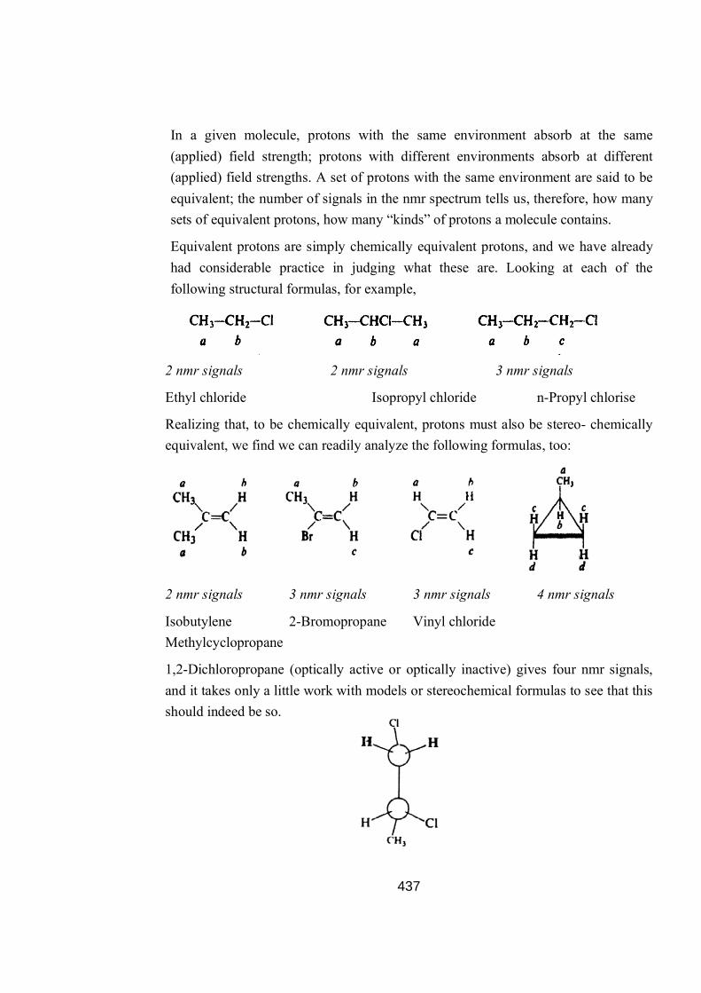
437

In a given molecule, protons with the same environment absorb at the same (applied) field strength; protons with different environments absorb at different (applied) field strengths. A set of protons with the same environment are said to be equivalent; the number of signals in the nmr spectrum tells us, therefore, how many sets of equivalent protons, how many “kinds” of protons a molecule contains.

Equivalent protons are simply chemically equivalent protons, and we have already had considerable practice in judging what these are. Looking at each of the following structural formulas, for example,

2 nmr signals 2 nmr signals 3 nmr signals

Ethyl chloride Isopropyl chloride n-Propyl chlorise

Realizing that, to be chemically equivalent, protons must also be stereo- chemically equivalent, we find we can readily analyze the following formulas, too:

2 nmr signals 3 nmr signals 3 nmr signals 4 nmr signals

Isobutylene 2-Bromopropane Vinyl chloride Methylcyclopropane

1,2-Dichloropropane (optically active or optically inactive) gives four nmr signals, and it takes only a little work with models or stereochemical formulas to see that this should indeed be so.

438

2 nmr signals

1,2-Dichloropropane

The product CH2Z—CH2Cl is the same regardless of which one of the three methyl protons is replaced. The (average) environment of the three protons is identical, and hence we expect one nmr signal for all three.

Replacement of either of the two methylene protons would give one of a pair of enantiomers: (Fig. 21.5)

Ethyl chloride

Fig. 21.5 Enantiotopic proton

Such pairs of protons are called enantiotopic protons. The environments of these two protons are mirror images of each other; these protons are equivalent, and we see one nmr signal for the pair. (Like any other physical property except rotation of polarized light—the nmr spectrum does not distinguish between mirror images.)

Turning to 2-bromopropene, we see that replacement of either of the vinylic protons gives one of a pair of diastereomers (geometric isomers, in this case):

Fig. 21.6 2-Bromopropane and Enantiotopic protons

Such pairs of protons are called diastereotopic protons. The environments of these two protons are neither identical nor mirror images of each other; these protons are non-equivalent, and we expect an nmr signal from each one.

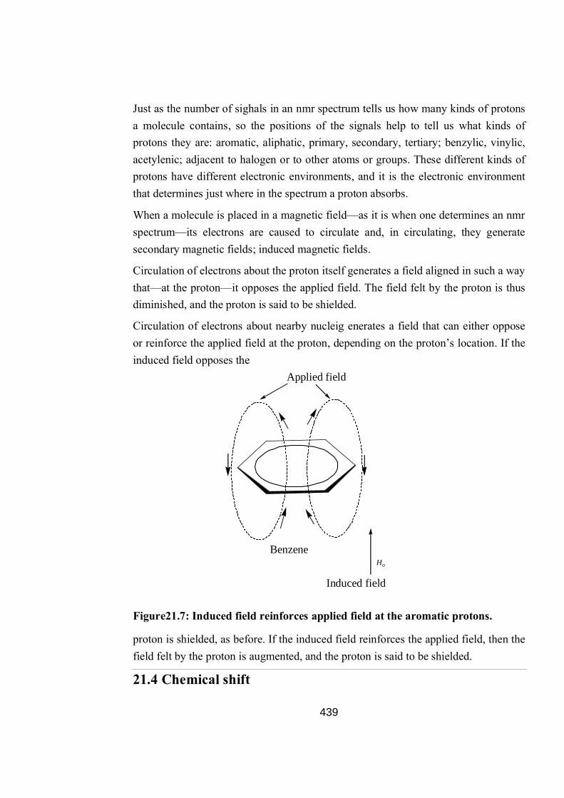
439

Just as the number of sighals in an nmr spectrum tells us how many kinds of protons a molecule contains, so the positions of the signals help to tell us what kinds of protons they are: aromatic, aliphatic, primary, secondary, tertiary; benzylic, vinylic, acetylenic; adjacent to halogen or to other atoms or groups. These different kinds of protons have different electronic environments, and it is the electronic environment that determines just where in the spectrum a proton absorbs.

When a molecule is placed in a magnetic field—as it is when one determines an nmr spectrum—its electrons are caused to circulate and, in circulating, they generate secondary magnetic fields; induced magnetic fields.

Circulation of electrons about the proton itself generates a field aligned in such a way that—at the proton—it opposes the applied field. The field felt by the proton is thus diminished, and the proton is said to be shielded.

Circulation of electrons about nearby nucleig enerates a field that can either oppose or reinforce the applied field at the proton, depending on the proton’s location. If the induced field opposes the

Figure21.7: Induced field reinforces applied field at the aromatic protons.

proton is shielded, as before. If the induced field reinforces the applied field, then the field felt by the proton is augmented, and the proton is said to be shielded.

21.4 Chemical shift

Induced field

Applied field

Ho

Benzene

440

Compared with a naked proton, a shielded proton requires a higher applied field strength and a deshielded proton requires a lower applied field strength to provide the particular effective field strength at which absorption occurs. Shielding shifts the absorption up field and deshielding shifts the absorption downfield. Such shifts in the position of nmr absorptions, arising from shielding and deshielding by electrons, are called chemical shifts. The unit in which a chemical shift is most conveniently expressed is parts per million (ppm) of the total applied magnetic field. Since shielding and deshielding arise from induced secondary fields, the magnitude of a chemical shift is proportional to the strength of the applied field or, what is equivalent, proportional to the radiofrequency the field must match. If, however, it is expressed as fraction ion of the applied field that is, if the observed shift is divided by the particular radiofrequency used then a chemical shift has a constant value that is independent of the radiofrequency and the magnetic field that the nmr spectrometer employs. The reference point from which chemical shifts are measured is, for practical reasons, not the signal from a naked proton, but the signal from an actual compound: usually tetramethylsilane (CH3)4Si. Because of the low electronegativity of silicon, the shielding of the protons in the silane is greater than in most other organic molecules; as a result, most nmr signals appear in the same direction from the tetramethylsilane signal.

The most commonly used scale is the δ (delta) scale. The position of the tetramethylsilane signal is taken as 0.0 ppm. Most chemical shifts have 8 values

between 0 and 10 (minus 10, actually). A small δ value represents a small downfield

shift, and a large δ value represents a large downfield shift. One commonly encounters another scale: the (tao) scale, on which the tetramethylsilane signal is taken as 10.0 ppm. Most i values lie between 0 and 10. The two scales are related by the expression

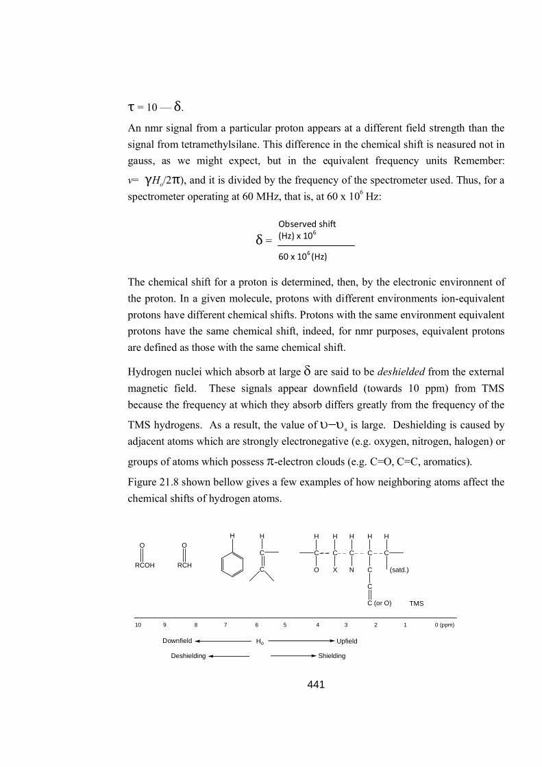
441

τ = 10 — δ.

An nmr signal from a particular proton appears at a different field strength than the signal from tetramethylsilane. This difference in the chemical shift is neasured not in gauss, as we might expect, but in the equivalent frequency units Remember:

v= γHo/2π), and it is divided by the frequency of the spectrometer used. Thus, for a spectrometer operating at 60 MHz, that is, at 60 x 106 Hz:

δ =

The chemical shift for a proton is determined, then, by the electronic environnent of the proton. In a given molecule, protons with different environments ion-equivalent protons have different chemical shifts. Protons with the same environment equivalent protons have the same chemical shift, indeed, for nmr purposes, equivalent protons are defined as those with the same chemical shift.

Hydrogen nuclei which absorb at large are said to be deshielded from the external magnetic field. These signals appear downfield (towards 10 ppm) from TMS because the frequency at which they absorb differs greatly from the frequency of the

TMS hydrogens. As a result, the value of s is large. Deshielding is caused by adjacent atoms which are strongly electronegative (e.g. oxygen, nitrogen, halogen) or

groups of atoms which possess -electron clouds (e.g. C=O, C=C, aromatics).

Figure 21.8 shown bellow gives a few examples of how neighboring atoms affect the chemical shifts of hydrogen atoms.

RCH

O

RCOH

OH

C

C

H

C

O

H

C

H

X

C

H

N

C

H

C

C

C (or O)

C

H

(satd.)

TMS

10 9 8 7 6 5 4 3 2 1 0 (ppm)

Downfield Upfield

ShieldingDeshielding

Ho

Observed shift (Hz) x 106

60 x 106 (Hz)

442

Fig. 21.8 Neighboring atoms affect

21.5 Continuous Wave (CW) NMR Spectrometer

Two types of NMR spectrometers are commonly encountered. They are:

(a) Continuous wave (CW) NMR spectrometer

(h) Fourier transform (FT) NMR spectrometer

We are going to discuss here continuous wave NMR spectrometer only.

(a) Continuous wvave (CW) NMR spectrometer:

The CW-NMR spectrometer detects the resonance frequencies of nuclei in a sample placed in a magnetic field by sweeping the frequency of RF radiation through a given range and directly recording the intensity of absorption as a function of frequency. The spectrum is usually recorded and plotted simultaneously with a recorder synchronized to the frequency of the RF source.

Fig. 21.9 illustrates a schematic diagram of a CW-NMR spectrometer. The essential features are described briefly as follows:

443

Figure 21.9 : Schematic diagram of CW-NMR spectrometer

(1) Powerful magnet annexed by a sweep generator:

The magnets used in NMR spectrometers are large permanent or electromagnets, capable of producing strong, stable and homogenous magnetic field (upto 2.5 Tesla or 25000 Gauss) over the area occupied by the sample. The development of superconducting solenoid magnets has considerably extended the practical limit of stable, homogenous magnetic fields upto about 12 Tesla, i.e., NMR spectrometers working at about 500 MHz (for protons) can now be dev iced. These magnets owe their remarkable strength to the superconducting properties of certain metals when cooled to extremely low temperatures (liquid helium. 3K). The magnet is controlled although the sample is held at the room temperature by being thermally isolated.

A very small air gap between the poles (about 3-5 inches) and also spinning of the sample between them serve as a source of homogenous magnetic field. The magnet

444

is further annexed by sweep generator in order to change the magnetic field precisely and continuously over a small range.

(2) The sample probe:

The sample probe is a device which holds the sample. Contained in the NMR tube in between two poles of the magnet, in the strongest and most homogenous part of the magnetic field. Apart from acting as holder, the probe has the following important functions.

(a) The transmission coil “bathes” the sample in radio frequency radiation of appropriate frequency say 200 MHz.

(b) The probe has another coil, the receiver coil, wrapped at right angles to the transmitter coil. This is the optimum angle for the detection of resonance.

(c) The probe permits the sample tube to be run, usually by an air jet directed towards a spinner turbine. Spinning the sample along one axis effectively increases the homogeneity of the magnetic field over the sample. Spinning the sample does lead to the formation of spinning side bands, appearing symmetrically on either side of the main spectral peaks and separated from them by the frequency of spinning.

(d) Finally, there can be other features in the probe, such as double resonance devices etc.

(iii) Radio frequency oscillator:

Radio frequencies are generated by electronic multiplication of natural frequency of a quartz crystal contained in a thermostated block. Different crystal sources and transmitters are used for different resonance frequencies. The radio frequency oscillator coil is installed perpendicular to the magnetic field and transmits radio waves of fixed frequency such as 60, 100, 200 or 300 MHz to a small coil that encircles the sample in the probe. The radio-frequency source is associated with a power controlling device so that level of RF power can be varied and adjusted empirically to get the best response.

(iv) Radio frequency receiver or detector:

The sample in the NMR probe gives information or data which has been detected as an analogue signal or voltage. Detectors, used in NMR spectrometers, are to be very sensitive as the signal levels are very small (less than 1 millivolt). Therefore, multiple amplification of the signals is required before they are fed to the output

445

devices. This amplification process is one source of electronic noise and contributes to low sensitivity of the NMR experiment.

The coil of RF receiver or detector is installed perpendicular both to the magnetic field and the oscillator coil, and is tuned to same frequency as the transmitter. When the precessional frequency is in unicon with the radio frequency, the nuclei induce an e.m.f. in the detector coil by virtue of the change in the magnetic flux following nuclear flip over. The signal is amplified and sent to recorder.

(v) Recorder and Integrator:

In routine analysis, the signal is usually sent directly to the recorder or oscilloscope. The oscilloscope is useful for fast scanning of the spectrum and allows preliminary adjustments to be made, e.g., setting optimum sensitivity or gain and electronic filtering of the signal.

The recorder records the spectrum as a plot of the resonance signal on the Y-axis (vertical) verses the strength of the magnetic field on the X-axis (horizontal). The strength of the resonance signal is directly proportional to the number of nuclei resonating at that field strength.

Most spectrometers are equipped with automatic integrators to measure the area under the observed signal. Such an area is proportional to the number of resonating nuclei giving the signal.

Sample preparation:

The first step in running a normal NMR spectrum is the complete dissolution of a requisite amount of the sample in the appropriate volume of a suitable NMR solvent. A brief description of the various commonly used NMR solvents is given below:

The commonly used NMR solvents:

(a) Carbon tetrachloride

Carbon tetrachioride, being aprotic and cheap, is an ideal solvent for proton spectra. However, its use is rather limited in practice to very non-polar compounds. It is hydrophobic is nature and consequently any moisture in a sample dissolved in this solvent will yield a turbid solution and thus impair homogeneity of the solution and consequently degrade resolution. Carbon tetrachloride does

446

have the advantage of being non-acidic and hence can be useful for certain acid-sensitive compounds.

(b) Deutero chloroform (CDCI3)

CDCI3 is the most useful NMR solvent and is liable to dissolve compounds of reasonably varying polarity, from non-polar to considerably polar; the small

residual CHCI3 signal at δ7.27 seldom causes a problem. CDCI3 being volatile, can easily be removed, so that recovery of the sample can be mode.

If a compound is only sparingly soluble in this solvent, DMSO-d6 may be added dropwise to increase the polarity of the solvent. It also causes the residual CHC13

to shift downfield to as low as 8.38 δ.

(c) Deutero dimethyl suphoxide (DMSO-d6)

DMSO-d6 is a very good solvent dissolving relatively insoluble heterocyclic compounds and salts. However, this solvent has the following disadvantages:

(i) It is very viscous and causes some degree of line broadening.

(ii) It is a mild oxidising agent and has been known to react with some compounds, particularly when warming the sample to obtain complete dissolution, as is often required with this solvent.

(iii) problems associated with restricted rotation become worse in DMSO-d6.

(iv) DMSO-d6 being relatively non-volatile, is difficult to remove from samples, one its recovery be required. The non-volatility, however, makes it the first choice for working at high temperature upto about 140°C.

(v) The main problem with this solvent is its affinity for water which makes it almost impossible to keep dry even if it is stored over molecular sieve.

(d) Deutero methanol (MeOH-d4)

MeOH-d4, a polar solvent, is suitable for running the NMR spectra of salts and extremely polar compounds. It has a very high affinity for water and is almost

impossible to keep dry. Its water peak is sharper and occurs around 4.86 δ

whereas the residual CD2HOD signal occurs near 3.3—3.23 δ.

The major disadvantage with MeOH-d4 is its susceptibility to exchange ionizable protons (e.g. -OH, -NH2 and even -CONH2) in the sample for deuterons and

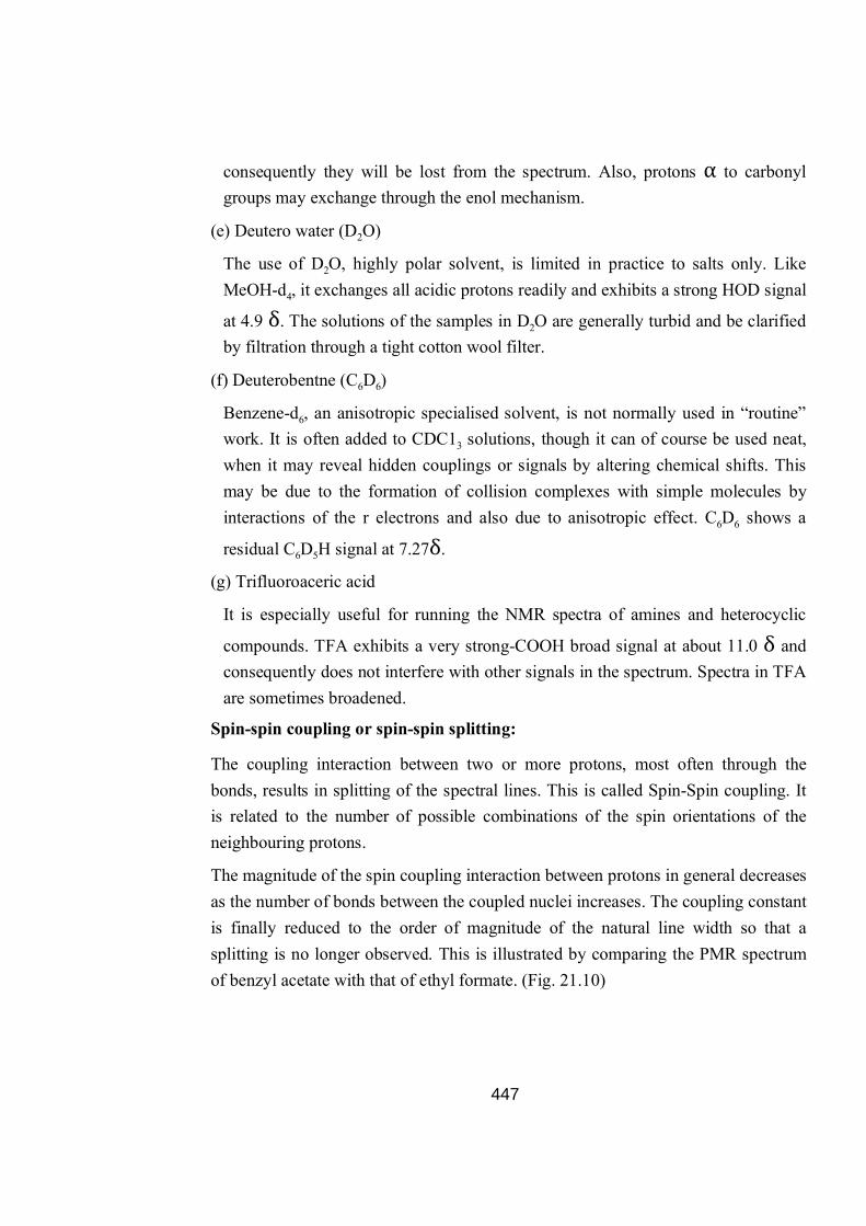
447

consequently they will be lost from the spectrum. Also, protons α to carbonyl groups may exchange through the enol mechanism.

(e) Deutero water (D2O)

The use of D2O, highly polar solvent, is limited in practice to salts only. Like MeOH-d4, it exchanges all acidic protons readily and exhibits a strong HOD signal

at 4.9 δ. The solutions of the samples in D2O are generally turbid and be clarified by filtration through a tight cotton wool filter.

(f) Deuterobentne (C6D6)

Benzene-d6, an anisotropic specialised solvent, is not normally used in “routine” work. It is often added to CDC13 solutions, though it can of course be used neat, when it may reveal hidden couplings or signals by altering chemical shifts. This may be due to the formation of collision complexes with simple molecules by interactions of the r electrons and also due to anisotropic effect. C6D6 shows a

residual C6D5H signal at 7.27δ.

(g) Trifluoroaceric acid

It is especially useful for running the NMR spectra of amines and heterocyclic

compounds. TFA exhibits a very strong-COOH broad signal at about 11.0 δ and consequently does not interfere with other signals in the spectrum. Spectra in TFA are sometimes broadened.

Spin-spin coupling or spin-spin splitting:

The coupling interaction between two or more protons, most often through the bonds, results in splitting of the spectral lines. This is called Spin-Spin coupling. It is related to the number of possible combinations of the spin orientations of the neighbouring protons.

The magnitude of the spin coupling interaction between protons in general decreases as the number of bonds between the coupled nuclei increases. The coupling constant is finally reduced to the order of magnitude of the natural line width so that a splitting is no longer observed. This is illustrated by comparing the PMR spectrum of benzyl acetate with that of ethyl formate. (Fig. 21.10)

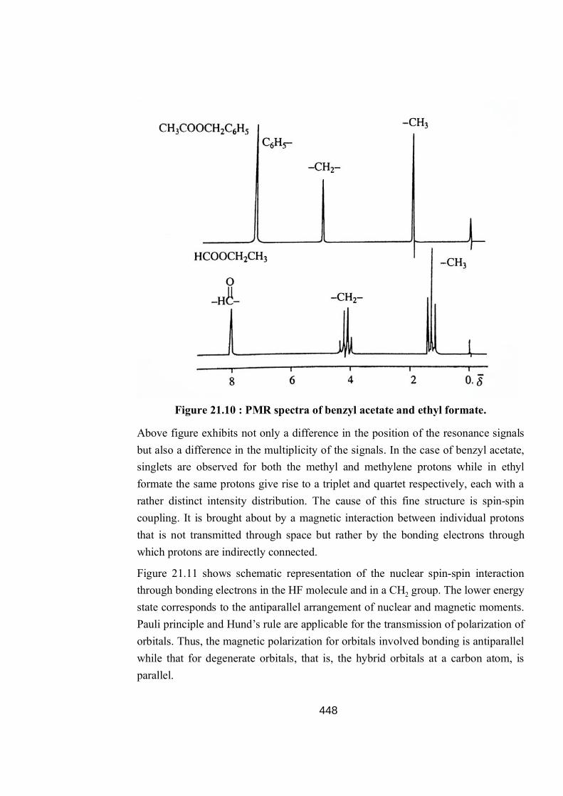
448

Figure 21.10 : PMR spectra of benzyl acetate and ethyl formate.

Above figure exhibits not only a difference in the position of the resonance signals but also a difference in the multiplicity of the signals. In the case of benzyl acetate, singlets are observed for both the methyl and methylene protons while in ethyl formate the same protons give rise to a triplet and quartet respectively, each with a rather distinct intensity distribution. The cause of this fine structure is spin-spin coupling. It is brought about by a magnetic interaction between individual protons that is not transmitted through space but rather by the bonding electrons through which protons are indirectly connected.

Figure 21.11 shows schematic representation of the nuclear spin-spin interaction through bonding electrons in the HF molecule and in a CH2 group. The lower energy state corresponds to the antiparallel arrangement of nuclear and magnetic moments. Pauli principle and Hund’s rule are applicable for the transmission of polarization of orbitals. Thus, the magnetic polarization for orbitals involved bonding is antiparallel while that for degenerate orbitals, that is, the hybrid orbitals at a carbon atom, is parallel.

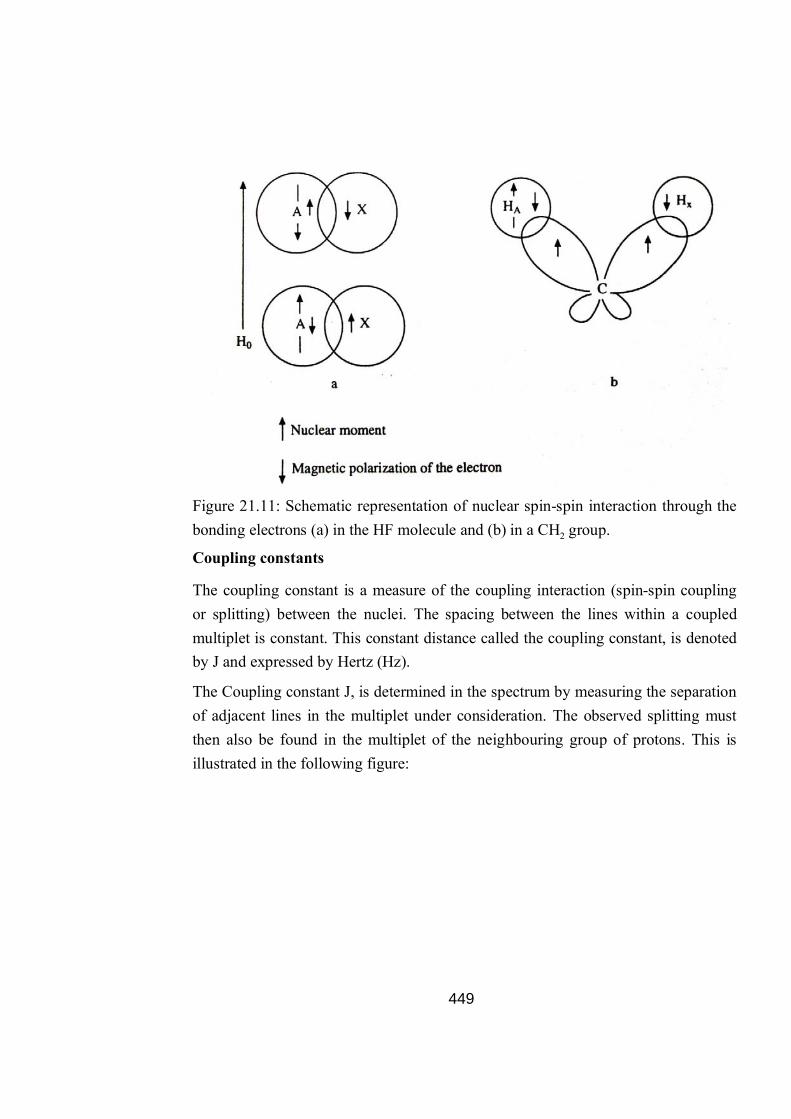
449

Figure 21.11: Schematic representation of nuclear spin-spin interaction through the bonding electrons (a) in the HF molecule and (b) in a CH2 group.

Coupling constants

The coupling constant is a measure of the coupling interaction (spin-spin coupling or splitting) between the nuclei. The spacing between the lines within a coupled multiplet is constant. This constant distance called the coupling constant, is denoted by J and expressed by Hertz (Hz).

The Coupling constant J, is determined in the spectrum by measuring the separation of adjacent lines in the multiplet under consideration. The observed splitting must then also be found in the multiplet of the neighbouring group of protons. This is illustrated in the following figure:

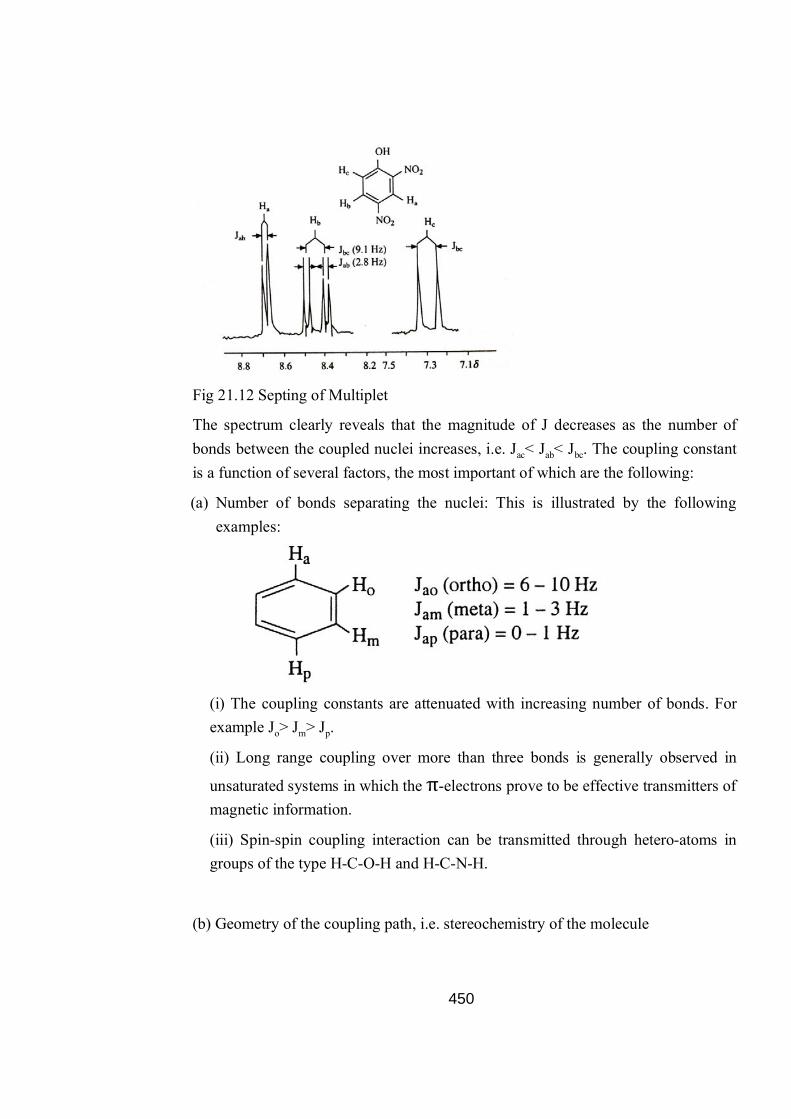
450

Fig 21.12 Septing of Multiplet

The spectrum clearly reveals that the magnitude of J decreases as the number of bonds between the coupled nuclei increases, i.e. Jac< Jab< Jbc. The coupling constant is a function of several factors, the most important of which are the following:

(a) Number of bonds separating the nuclei: This is illustrated by the following examples:

(i) The coupling constants are attenuated with increasing number of bonds. For example Jo> Jm> Jp.

(ii) Long range coupling over more than three bonds is generally observed in

unsaturated systems in which the π-electrons prove to be effective transmitters of magnetic information.

(iii) Spin-spin coupling interaction can be transmitted through hetero-atoms in groups of the type H-C-O-H and H-C-N-H.

(b) Geometry of the coupling path, i.e. stereochemistry of the molecule

451

By observing some typical values of H-H coupling constants in organic compounds it can be easily observed that the magnitude of coupling constants for protons in general lies in the range 5-17 Hz and that these parameters are very sensitive to the geometry of the coupling path, i.e. the stereochemistry of the molecule. For example Jtrans is, in general, greater than Jcis. In cyclopropane, however, Jcis> Jtrans.Similarly in cyclohexane Jaa> Jee.

21.6 Application of NMR spectroscopy in structure determination

a. n-Pentane: (Fig. 21.13)

1. A triplet at 0.906 δ, equivalent to 6 H, exhibits the presence of terminal methyl protons (a).

2. A multiplet centred at 1.286 δ, due to six equivalent protons (b) indicates three CH2 groups linked to methyl groups on either side.

Fig. 12.13 NMR spentrs of n-Pentane

b. Ethyl benzene: (21.14)

1. A triplet (J = 9 Hz) at 1.20 δ, equivalent to 3H, represents methyl protons (a).

2., A quartet (J = 9 Hz) at 2.61 δ, equivalent to 2H, indicates methylëne protons (b). They are deshielded because they are attached to the benzene ring. (The 3H upfield triplet and 2H down quartet indicate the ethyl group).

452

3. The signals from five protons on the phenyl ring occur at the same place (7.12

δ. and characteristic of five aromatic protons of a monosubstituted benzene with a non electro negative substituent.

Fig. 21.14 NMR Cpectra of Ethyl benzene:

c. Methylstyrene: (Fig. 21.15)

1. A 3H (dd) at 2.11 δ indicates the methyl protons (a) which has allylic coupling with proton ‘b’ (J = 1.6 Hz) and also with proton ‘c’ (J = 0.8 Hz).

2. A 1H (dq) at 5.05 δ exhibits the proton (b) which is split by the methyl group into a quartet (Jab = 1.6 Hz) and finally into a doublet of quartet by the proton (c).

3. A 1H (dq) at 5.34 δ, similarly represents the proton (c).

4. A multiplet at 7.34 δ, equivalent to five aromatic protons (d) exhibits a monosubstituted benzene ring.

453

Fig 21.16 NMR Cpeitrs of Methylstyrene

d. Phenylacetylene: (Fig. 21.16)

1. A singlet at 2.98 δ, equivalent to 1H, indicates the acetylenic proton (CC—H).

2. A multiplet centred at 7.40 δ, equivalent to five aromatic protons, represents monosubstituted benzene ring.

Fig. 21.16 NMR Cpetrs of Phonoyl acetybre

e. 1,1,2- Trichloromethane: (Fig. 21.17)

1. A doublet centred at 3.95 δ, equivalent to 2H, indicates the methylene protons (a).

2. The methine proton, being adjacent to two chlorine atoms, resonates at lower field as compared to two methylene protons which are adjacent to one chlorine

atom, consequently a triplet centred at 5.77 δ, equivalent to 1H, represents the methine proton (b).

454

Fig 21.17 NMR Cpiha of 1,1,T4chlo20 methone

f. Ethyl iodide: (Fig 21.18)

1. A triplet (J = 6 Hz) centred at 1.8 δ, equivalent to 3H, indicates the methyl protons (a).

2. A quartet (J = 6 Hz) centred at 3.2 δ, equivalent to 2H, indicates the methylene protons (b). (The 3H upfield triplet and 2H downfield quartet indicate the ethyl group).

Fig 21.18 NMR Cpettra of ethyl iodide

g. Ethyl alcohol: (Fig 21.19)

1. A triplet centred at 1.18 δ, equivalent to 3H, represents the methyl protons (a).

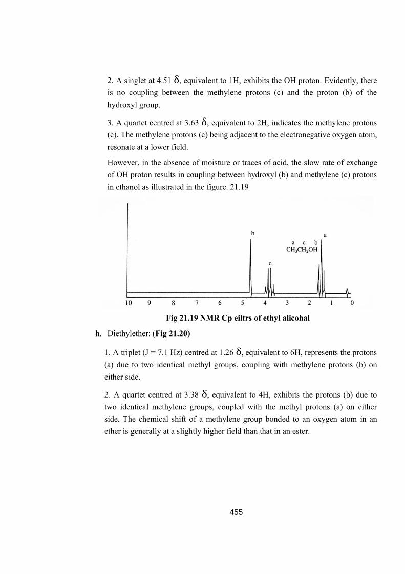
455

2. A singlet at 4.51 δ, equivalent to 1H, exhibits the OH proton. Evidently, there is no coupling between the methylene protons (c) and the proton (b) of the hydroxyl group.

3. A quartet centred at 3.63 δ, equivalent to 2H, indicates the methylene protons (c). The methylene protons (c) being adjacent to the electronegative oxygen atom, resonate at a lower field.

However, in the absence of moisture or traces of acid, the slow rate of exchange of OH proton results in coupling between hydroxyl (b) and methylene (c) protons in ethanol as illustrated in the figure. 21.19

Fig 21.19 NMR Cp eiltrs of ethyl alicohal

h. Diethylether: (Fig 21.20)

1. A triplet (J = 7.1 Hz) centred at 1.26 δ, equivalent to 6H, represents the protons (a) due to two identical methyl groups, coupling with methylene protons (b) on either side.

2. A quartet centred at 3.38 δ, equivalent to 4H, exhibits the protons (b) due to two identical methylene groups, coupled with the methyl protons (a) on either side. The chemical shift of a methylene group bonded to an oxygen atom in an ether is generally at a slightly higher field than that in an ester.

456

Fig 21.20 NMR Cpectrs of Di ethyl ether

i. Acetaldehyde: (Fig 21.21)

1. A doublet (Jab = 2.8 Hz) centred at 2.14 δ, equivalent to 3H, represents the methyl protons (a).

2. A quartet, centred at 9.78 δ, equivalent to 1H, indicates the aldehydic proton (b).

Fig 21.21 NMR Cpeiths of Acet aldehyde

j. Cinnamaldehyde: (Fig 21.222)

1. A doublet of doublet centred at 6.62 δ, equivalent to 1H (Ha) is due to the vicinal (J = 7.4 Hz)and trans coupling (J = 16.3Hz) of Ha with Hd and Hb respectively

457

2. 2. A doublet (J = 16.3 Hz) at 6.75 δ, equivalent of 1H (Hb), is due to the trans coupling with proton Ha.

3. 3. A multiplet at 7.40 δ, equivalent to 5 aromatic protons (c) indicates monosubstitu ted benzene ring

4. 4. A doublet (J = 7.41 Hz) at 9.66 δ, equivalent of 1H (proton d) indicates the aldehydic proton (Hd).

Fig 21.22 NMR Cpento ci nnamaldhyde

k. Acetophenone: (Fig 21.23)

1. A singlet at 2.47 δ, equivalent to 3H, represents the methyl protons (a), attached to benzoyl group.

2. Two separate downfield multiplets centred at 7.50 δ and 7.90 δ, exhibit respectively the aromanc protons b and c. The ortho-protons (c) are deshielded by the diamagnetic anisotropic effect of CO group. The upfield multiplet indicates the three (b) protons.

458

Fig 21.23 NMR of Aceto phenone

l. Benzoic acid: (Fig 21.24)

1. A multiplet at 7.50—7.70 δ, equivalent to 3H, is due to the aromatic protons (b).

2. A multiplet at 8.10—8.30 δ, equivalent to 2H, is due to the aromatic protons (a).

3. A singlet at 12.70 δ, equivalent to 1H, is due to the carboxylic acid proton (c).

Fig 21.24 NMR of Benzine acid

m. Acetic anhydyride: (Fig 21.25)

A singlet at 2.18 δ, equivalent to 6H.indicates two identical methyl groups.

459

Fig 21.26 NMR of acetre anhydirde

n. Acetanilide: Fig 21.25

1. A singlet at 2.09 δ, equivalent to 3H, indicates the methyl protons (a).

2. A distorted singlet at 3.09 δ, equivalent to 1H, is due to the amide proton (b) (shifted upfield by the solvent).

3. A multiplet at 7.27 δ, equivalent to 3H, exhibits the aromatic protons (c).

4. A multiplet at 7.75 δ, equivalent to 2H, represents the aromatic protons (d).

Fig 21.26 NMR of Acatanilide

460

o. Diethylamine: Fig 21.27

1. A singlet at 0.60 δ, equivalent to 1H, is due to the amine proton (c) (exchangeable with D2O).

2. A triplet (Jab = 7.3 Hz) at 1.05 δ, equivalent to 6H, indicates protons (a) due to two identical methyl groups.

3. A quartet at 2.61 δ, equivalent to 4H, exhibits protons (b) due to two identical methylene groups.

Fig 21.28 NMR of diethyl amine

Another NMR spectroscopy application:

NMR has found some use in the medical field, where large nuclear magnetic resonance spectrometers are set up so that people can be used as samples. A patient is placed in a magnetic field and bombarded with harmless radio waves. NMR signals from the protons in the tissues can be analyzed. In this way, the status of the bodily tissues can be determined, and with the computer control that is available, medical doctors can obtain many perspectives of the tissues inside a patient without any sort of invasive procedures. Problems like tumors, spinal irregularities, and cardiovascular disease can be evaluated without harm to the patient. However, in the medical field the technique is referred to as magnetic resonance imaging, or MRI. Apparently the word “nuclear” is dropped because of its connotations. Be that as it may, MRI is still NMR, a nuclear spin phenomenon.

20.1 Choose the correct attention :-- (After 21.6)

461

a) How many NMR signals one formed in 2 chloropropene

i. 2 ii 3 iii 1 iv None

b) Cluive multiplicity of signals CH3 CH2 OCH2 CH3 NMR

i Two Triplets ii a Triplets and a quartet iii Three singlets

iv Two singlets and two triplets

c) which of the following solvents can not be used in NMR spectroscopy:-

i CCL 4 ii CS2 iii CH CL iv all

d) The spin is an integer 1,2,3,--------- for a nucleus having

i even number of protons and neutrons ii odd mass number

iii even mass number and odd number of protons iv None

(e) NMR spectra is observed in -------- region

(i) radio frequency (ii) micro wave (iii) UV/VIS (iv) X- Rays

(f) The signals for a compound like A—CH2 – CH2 –B will be

(i) two triplets (ii) two singlets (iii) one singlets (iv) all

21.7 Summary

NMR spectroscopy is one of the most important technique for the structure determination of the organic compounds. This chapter deals with the basic principales and application of nuclear magnetic resonance spectroscopy and hence can be very useful for an chemist.

In this chapter spin active nuclei, chemical shift, spin-spin coupling, coupling constant, NMR spectrometer and various examples of structure elucidation of organic compounds have been discussed.


462

1. Write short note on NMR spectroscopy. 2. Discuss the basic principle of NMR spectroscopy. 3. What do you mean by Larmor frequency? 4. What do you mean by spin active nuclei? 5. Write down the relaxation phenomenon in NMR spectroscopy. 6. Write detailed notes on number of signals in NMR spectroscopy. 7. Discuss the chemical shift in detail. 8. Describe NMR spectrometer. 9. Discuss the application of NMR spectroscopy in structure elucidation with

examples.

21.9 Glossary

Chemical shift:-- Deference in the resonance frequency of a given proton

compared to that of methyl proton of tatia methyl silence (TMS)

Aniso tropic effect:- magnetic field associated with the election circulation in

molecules containing in bond.

Shielding:-- Effective magnetic field experienced by the nucleus is less than

that of field , nucleus is land to be Aniston tropic.

Spin –spin spilting:- spilting between nucleric with different chemical shift.

Coupling content :-- measure of coupling intentation between the nuclei.

21.1Answer to say assessment questions

(a) (ii), (b) (ii), (c) (iii), (d) (iii) (e) (i) (f) (i)


VARDHMAN MAHAVEER OPEN UNIVERSITYassets.vmou.ac.in/MSCCH03.pdf · 2014-11-01 · decreases. (iii)...

Documents

Transcript of VARDHMAN MAHAVEER OPEN UNIVERSITYassets.vmou.ac.in/MSCCH03.pdf · 2014-11-01 · decreases. (iii)...