Vapnik-Chervonenkis Densityin Model Theory

Matthias AschenbrennerUniversity of California, Los Angeles

(joint with A. Dolich, D. Haskell, D. Macpherson, and S. Starchenko)

VC dimension and VC density

Let (X,S) be a set system, i.e., X is a set (the base set), andS is a collection of subsets of X. (We sometimes also speak ofa set system S on X.)

Given A ⊆ X, we let

S ∩A := {S ∩A : S ∈ S}

and call (A,S ∩A) the set system on A induced by S.

We say A is shattered by S if S ∩A = 2A.

If S 6= ∅, then we define the VC dimension of S, denoted byVC(S), as the supremum (in N ∪ {∞}) of the sizes of all finitesubsets of X shattered by S. We also decree VC(∅) := −∞.

VC dimension and VC density

Examples

1 X = R, S = all unbounded intervals. Then VC(S) = 2.2 X = R2, S = all halfspaces. Then VC(S) = 3.

One point in the convex hullof the others

No point in the convex hullof the others

3 Let S = half spaces in Rd. Then VC(S) = d+ 1.(The inequality 6 follows from Radon’s Lemma.)

VC dimension and VC density

Examples (continued)

4 X = R2, S = all convex polygons. Then VC(S) =∞.

(But VC({convex n-gons in R2}) = 2n+ 1.)

VC dimension and VC density

The function

n 7→ πS(n) := max

{|S ∩A| : A ∈

(X

n

)}: N→ N

is called the shatter function of S. Then

VC(S) = sup{n : πS(n) = 2n

}.

One says that S is a VC class if VC(S) <∞.

The notion of VC dimension wasintroduced by Vladimir Vapnik andAlexey Chervonenkis in the early1970s, in the context ofcomputational learning theory.

VC dimension and VC density

A surprising dichotomy holds for πS :

The Sauer-Shelah dichotomy

Either• πS(n) = 2n for every n (if S is not a VC class),

or• πS(n) 6

(n6d

):=(n0

)+ · · ·+

(nd

)where d = VC(S) <∞.

One may now define the VC density of S as

vc(S) =

{inf{r ∈ R>0 : πS(n) = O(nr)} if VC(S) <∞∞ otherwise.

We also define vc(∅) := −∞.

VC dimension and VC density

Examples

1 S =(X6d

). Then VC(S) = vc(S) = d; in fact πS(n) =

(n6d

).

2 S = half spaces in Rd. Then VC(S) = d+ 1, vc(S) = d.

VC density is often the right measure for the combinatorialcomplexity of a set system.

Some basic properties:

• vc(S) 6 VC(S), and if one is finite then so is the other;• VC(S) = 0⇐⇒ |S| = 1;• S is finite⇐⇒ vc(S) = 0⇐⇒ vc(S) < 1;• S = S1 ∪ S2 ⇒ vc(S) = max{vc(S1), vc(S2)}.

VC duality

Let X be a set (possibly finite). Given A1, . . . , An ⊆ X, denoteby S(A1, . . . , An) the set of atoms of the Boolean subalgebra of2X generated by A1, . . . , An: those subsets of X of the form⋂

i∈IAi ∩

⋂i/∈I

X \Ai where I ⊆ {1, . . . , n}

which are non-empty (= “the non-empty sets in the Venndiagram of A1, . . . , An”).

Suppose now that S is a set system on X. We define

n 7→ π∗S(n) := max{|S(A1, . . . , An)| : A1, . . . , An ∈ S

}: N→ N.

We say that S is independent (in X) if π∗S(n) = 2n for every n,and dependent (in X) otherwise.

VC duality

Example (X = R2, S = half planes in R2)

π∗S(n) =

{maximum number of regions into which n halfplanes partition the plane.

Adding one half plane to n− 1 given half planes divides at mostn of the existing regions into 2 pieces. So π∗S(n) = O(n2).

The function π∗S is called the dual shatter function of S.

VC duality

Let X, Y be infinite sets, Φ ⊆ X × Y a binary relation. Put

SΦ := {Φy : y ∈ Y } ⊆ 2X where Φy := {x ∈ X : (x, y) ∈ Φ},

andπΦ := πSΦ

, π∗Φ := π∗SΦ,

VC(Φ) := VC(SΦ), vc(Φ) := vc(SΦ).

We also write

Φ∗ ⊆ Y ×X :={

(y, x) ∈ Y ×X : (x, y) ∈ Φ}.

In this way we obtain two set systems: (X,SΦ) and (Y,SΦ∗)

Given a finite set A ⊆ X we have a bijection

A′ 7→⋂x∈A′

Φ∗x ∩⋂

x∈A\A′Y \ Φ∗x : SΦ ∩A→ S(Φ∗x : x ∈ A).

VC duality

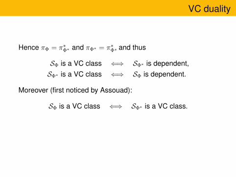
Hence πΦ = π∗Φ∗ and πΦ∗ = π∗Φ, and thus

SΦ is a VC class ⇐⇒ SΦ∗ is dependent,SΦ∗ is a VC class ⇐⇒ SΦ is dependent.

Moreover (first noticed by Assouad):

SΦ is a VC class ⇐⇒ SΦ∗ is a VC class.

The model-theoretic context

We fix:L: a first-order language,

x = (x1, . . . , xm): object variables,y = (y1, . . . , yn): parameter variables,

ϕ(x; y): a partitioned L-formula,M : an infinite L-structure, andT : a complete L-theory without finite models.

The set system (on Mm) associated with ϕ in M :

SMϕ := {ϕM (Mm; b) : b ∈Mn}

If M ≡N , then πSMϕ = πSNϕ . So, picking M |= T arbitrary, set

πϕ := πSMϕ , VC(ϕ) := VC(SMϕ ), vc(ϕ) := vc(SMϕ ).

The model-theoretic context

The dual of ϕ(x; y) is ϕ∗(y;x) := ϕ(x; y). Put

VC∗(ϕ) := VC(ϕ∗), vc∗(ϕ) := vc(ϕ∗).

We have π∗ϕ = πϕ∗ , hence VC∗(ϕ) and vc∗(ϕ) can be computedusing the dual shatter function of ϕ.

If VC(ϕ) <∞ then we say that ϕ is dependent in T . Thetheory T does not have the independence property (is NIP) ifevery partitioned L-formula is dependent in T .

An important theorem of Shelah (given other proofs byLaskowski and others) says that for T to be NIP it is enough forfor every L-formula ϕ(x; y) with |x| = 1 to be dependent.

Many (but not all) well-behaved theories arising naturally inmodel theory are NIP.

The model-theoretic context

Some questions about vc in model theory

1 Possible values of vc(ϕ). There exists a formula ϕ(x; y) inLrings with |y| = 4 such that

vcACF0(ϕ) = 43 ; vcACFp(ϕ) = 3

2 for p > 0.

We do not know an example of a formula ϕ in a NIP theorywith vc(ϕ) /∈ Q.

2 Growth of πϕ. There is an example of an ω-stable T and anL-formula ϕ(x; y) with |y| = 2 and

πϕ(n) = 12n log n (1 + o(1)).

3 Uniform bounds on vc(ϕ).

Uniform bounds on VC density

Some reasons why it should be interesting to obtain bounds onvc(ϕ) in terms of |y| = number of free parameters:

1 uniform bounds on VC density often “explain” why certainbounds on the complexity of geometric arrangements,used in computational geometry, are polynomial in thenumber of objects involved;

2 connections to strengthenings of the NIP concept: ifvc(ϕ) < 2 for each ϕ(x; y) with |y| = 1 then T is dp-minimal.

Uniform bounds on VC density

TheoremSuppose T expands the theory of linearly ordered sets, andassume that T is weakly o-minimal, i.e., in every M |= T ,every definable subset of M is a finite union of convex subsetsof M . Then for each ϕ(x; y) we have πϕ(t) = O(t|y|), hencevc(ϕ) 6 |y|.

• Generalizes results due to Karpinski-Macintyre and Wilkie;• Idea of the proof:

• generalize definition of π∗ϕ to finite sets ∆ of formulas

instead of a single ϕ;• the number of parameters needed in a uniform definition of

∆-types over finite parameter sets yields a bound on π∗∆(t);

• reduce to the case where |x| = 1 and each instance ofϕ ∈ ∆ defines an initial segment, in which case each finite∆-type can be defined by a single parameter.

Uniform bounds on VC density

Interesting classes of NIP theories are provided by certainvalued fields. By a non-trivial elaboration of our methods:

TheoremSuppose M = Qp is the field of p-adic numbers, construed as astructure in the language of rings. Then vc(ϕ) 6 2|y| − 1.

We also have uniform bounds on VC density (obtained by othertechniques) for certain stable structures; e.g., we characterizethose abelian groups for which we have such uniform bounds.

There are many open questions in this subject.

Open question

If there is some d1 such that vc(ϕ) 6 d1 for each ϕ(x; y) with|y| = 1, is there is some dm such that vc(ϕ) 6 dm for eachϕ(x; y) with |y| = m?

From Lipschitz maps to VC density

QuestionLet f : A→ Rn, A ⊆ Rm, be L-Lipschitz (where L ∈ R>0), i.e.,

||f(x)− f(y)|| 6 L · ||x− y|| for all x, y ∈ A.

Can one extend f to an L-Lipschitz map Rm → Rn?

Kirszbraun (1934): yes for all n

There always exists an L-Lipschitz extension Rm → Rn of f .

The usual proofs of this theorem all use some sort of transfiniteinduction.

From Lipschitz maps to VC density

Question (Chris Miller)

Let f : A→ Rn, A ⊆ Rm, be L-Lipschitz and semialgebraic. Isthere a semialgebraic L-Lipschitz map Rm → Rn extending f?

More generally, one may ask this for Lipschitz maps definablein an o-minimal expansion R = (R, 0, 1,+,×, <, . . . ) of a realclosed field R, instead of R = (R, 0, 1,+,×, <).

Why is this extra generality interesting?

• no “higher-order” Tarski principle for transfer fromo-minimal expansions of R to R;

• brings out the inherent uniformities in the construction.

In fact, o-minimality even turns out to be an unnecessarilystrong assumption.

From Lipschitz maps to VC density

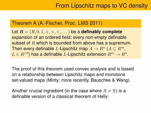
Theorem A (A.-Fischer, Proc. LMS 2011)

Let R = (R, 0, 1,+,×, <, . . . ) be a definably completeexpansion of an ordered field: every non-empty definablesubset of R which is bounded from above has a supremum.Then every definable L-Lipschitz map A→ Rn (A ⊆ Rm,L ∈ R>0) has a definable L-Lipschitz extension Rm → Rn.

The proof of this theorem used convex analysis and is basedon a relationship between Lipschitz maps and monotoneset-valued maps (Minty; more recently, Bauschke & Wang).

Another crucial ingredient (in the case where R 6= R) is adefinable version of a classical theorem of Helly:

From Lipschitz maps to VC density

Theorem B (A.-Fischer, Proc. LMS 2011)

Let R be a definably complete expansion of an ordered field.Let C be a definable family of closed bounded convex subsetsof Rn. Suppose C is (n+ 1)-consistent:⋂

C′ 6= ∅ for all C′ ⊆ C with |C′| 6 n+ 1.

Then⋂C 6= ∅.

Our proof of this theorem uses an optimization argument.

S. Starchenko pointed out that in the case of an o-minimal R,our theorem follows from an analysis of the model-theoreticnotion of forking in o-minimal structures due to A. Dolich.

From Lipschitz maps to VC density

A subset T of X is called a transversal of a set system S on Xif every member of S contains an element of T .

Theorem (Dolich ’04, made explicit by Peterzil & Pillay ’07)

Let R be an o-minimal expansion of a real closed field, and letC = {Ca}a∈A be a definable family of closed and boundedsubsets of Rn parameterized by a subset A of Rm. If C isN(m,n)-consistent, where

N(m,n) = (1 + 2m) · (1 + 22m) · · · (n factors),

then C has a finite transversal.

From Lipschitz maps to VC density

QuestionCan one do better than the bound N(m,n)?

Theorem (Matoušek, 2004)

Let (X,S) be a set system of finite dual VC density vc∗(S).Suppose S is d-consistent, where d > vc∗(S). Assume that Xcomes equipped with a topology making all sets in S compact.Then S has a finite transversal.

Corollary

Let R be an o-minimal structure on R, and let C = {Ca}a∈A bea definable family of compact subsets of Rn. If C is(n+ 1)-consistent, then C has a finite transversal.

From Lipschitz maps to VC density

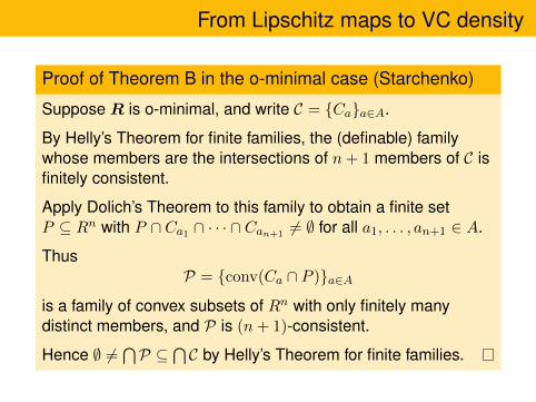
Proof of Theorem B in the o-minimal case (Starchenko)

Suppose R is o-minimal, and write C = {Ca}a∈A.

By Helly’s Theorem for finite families, the (definable) familywhose members are the intersections of n+ 1 members of C isfinitely consistent.

Apply Dolich’s Theorem to this family to obtain a finite setP ⊆ Rn with P ∩ Ca1 ∩ · · · ∩ Can+1 6= ∅ for all a1, . . . , an+1 ∈ A.

ThusP = {conv(Ca ∩ P )}a∈A

is a family of convex subsets of Rn with only finitely manydistinct members, and P is (n+ 1)-consistent.

Hence ∅ 6=⋂P ⊆

⋂C by Helly’s Theorem for finite families.