Vapnik-Chervonenkis Dimension

Part I: Definition and Lower bound

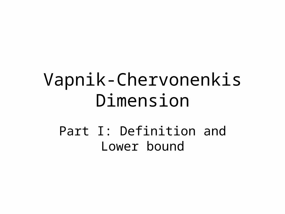
PAC Learning model

• There exists a distribution D over domain X• Examples: <x, c(x)>

– use c for target function (rather than ct)

• Goal: – With high probability (1-)– find h in H such that – error(h,c ) < – arbitrarily small.

VC: Motivation

• Handle infinite classes.

• VC-dim “replaces” finite class size.

• Previous lecture (on PAC):– specific examples– rectangle.– interval.

• Goal: develop a general methodology.

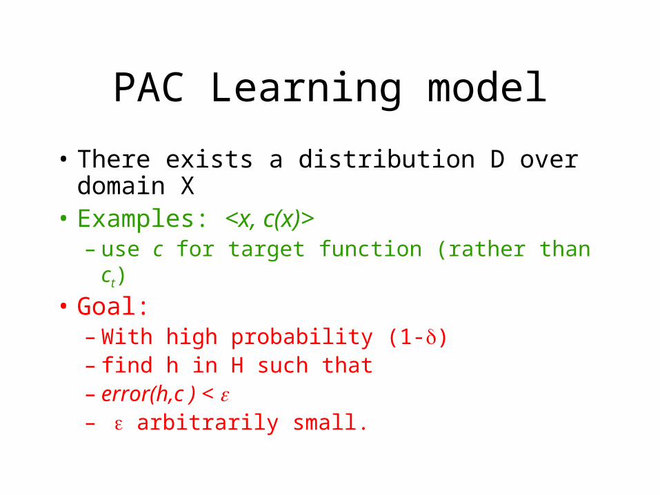
Definitions: Projection

• Given a concept c over X– associate it with a set (all positive examples)

• Projection (sets)– For a concept class C and subset S– C(S) = { c S | c C}

• Projection (vectors)– For a concept class C and S = {x1, … , xm}– C(S) = {<c(x1), … , cxm)> | c C}

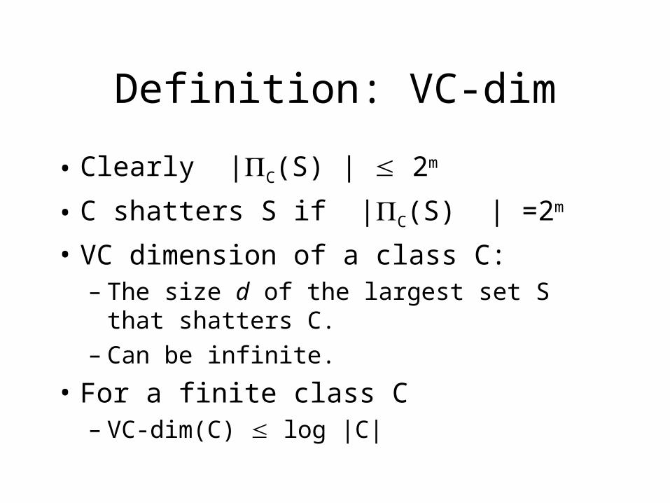
Definition: VC-dim

• Clearly |C(S) | 2m

• C shatters S if |C(S) | =2m

• VC dimension of a class C:– The size d of the largest set S that shatters C.– Can be infinite.

• For a finite class C– VC-dim(C) log |C|

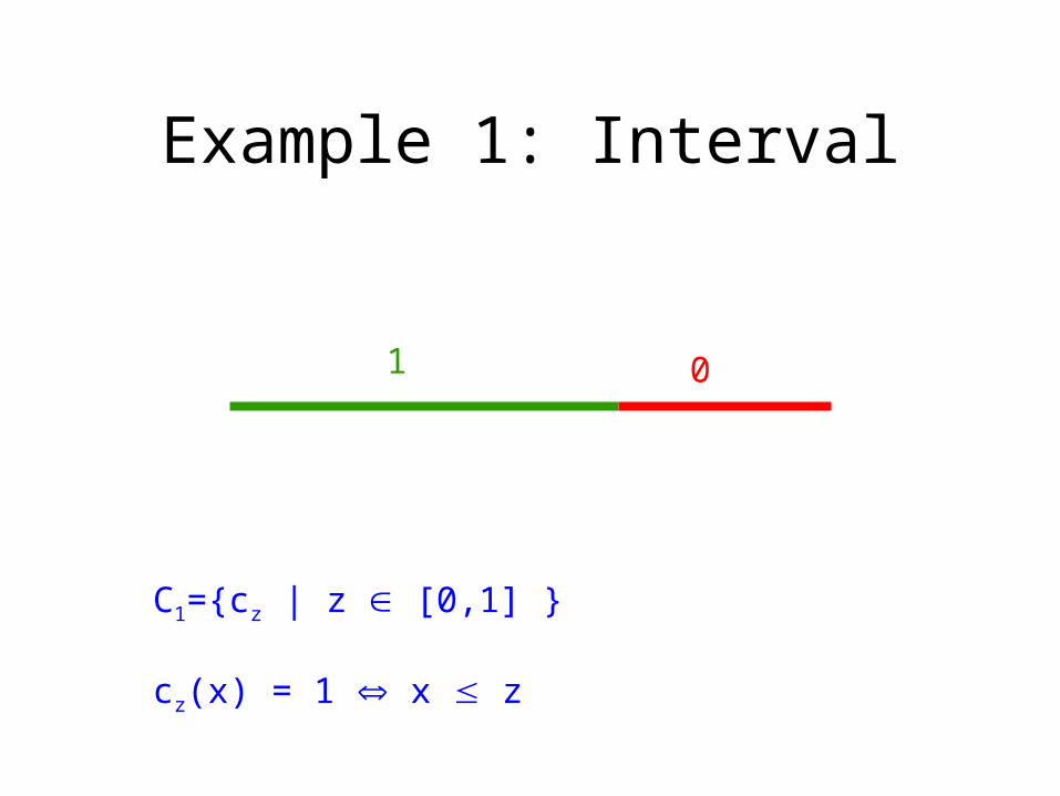
Example 1: Interval

1 0

C1={cz | z [0,1] }

cz(x) = 1 x z

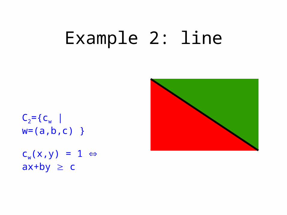
Example 2: line

C2={cw | w=(a,b,c) }

cw(x,y) = 1 ax+by c

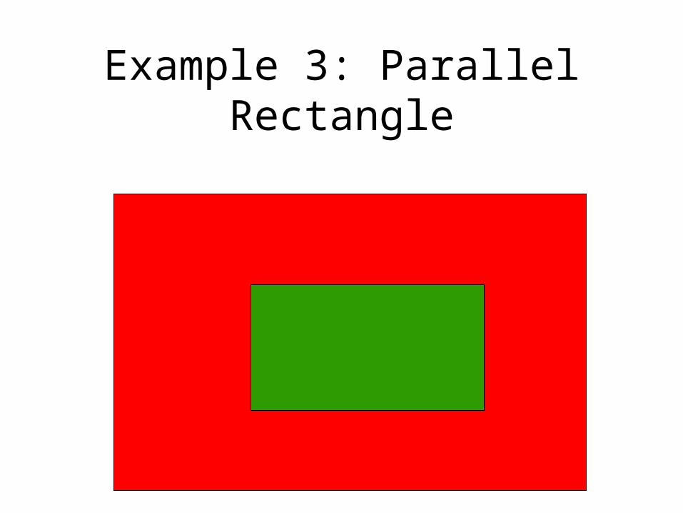
Example 3: Parallel Rectangle

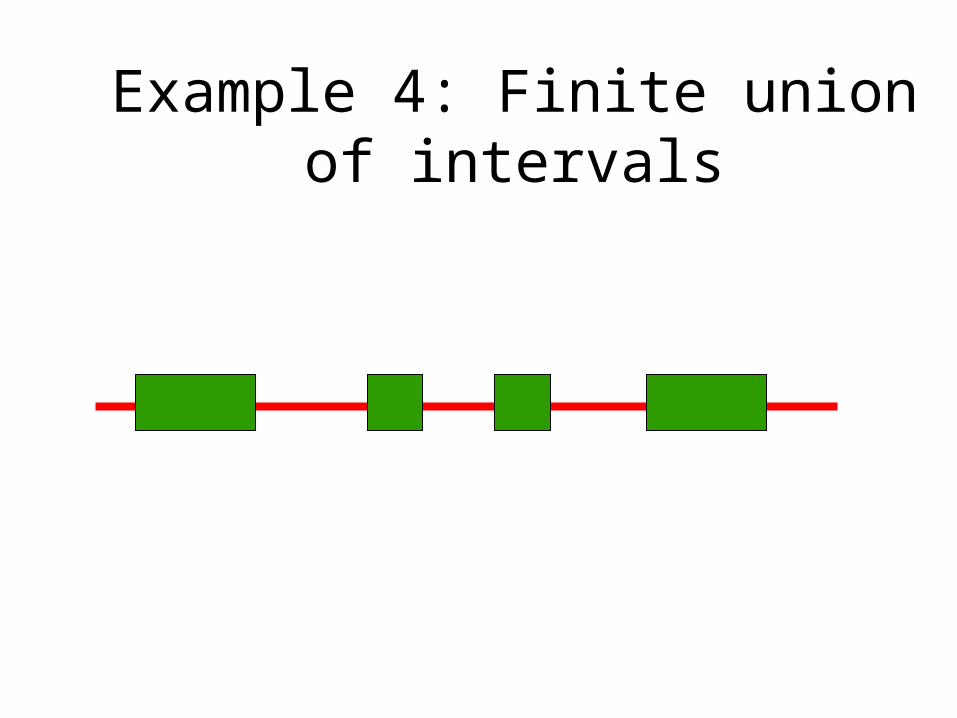
Example 4: Finite union of intervals

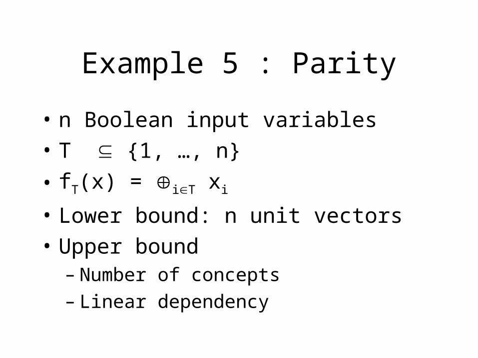
Example 5 : Parity

• n Boolean input variables

• T {1, …, n}

• fT(x) = iT xi

• Lower bound: n unit vectors

• Upper bound– Number of concepts– Linear dependency

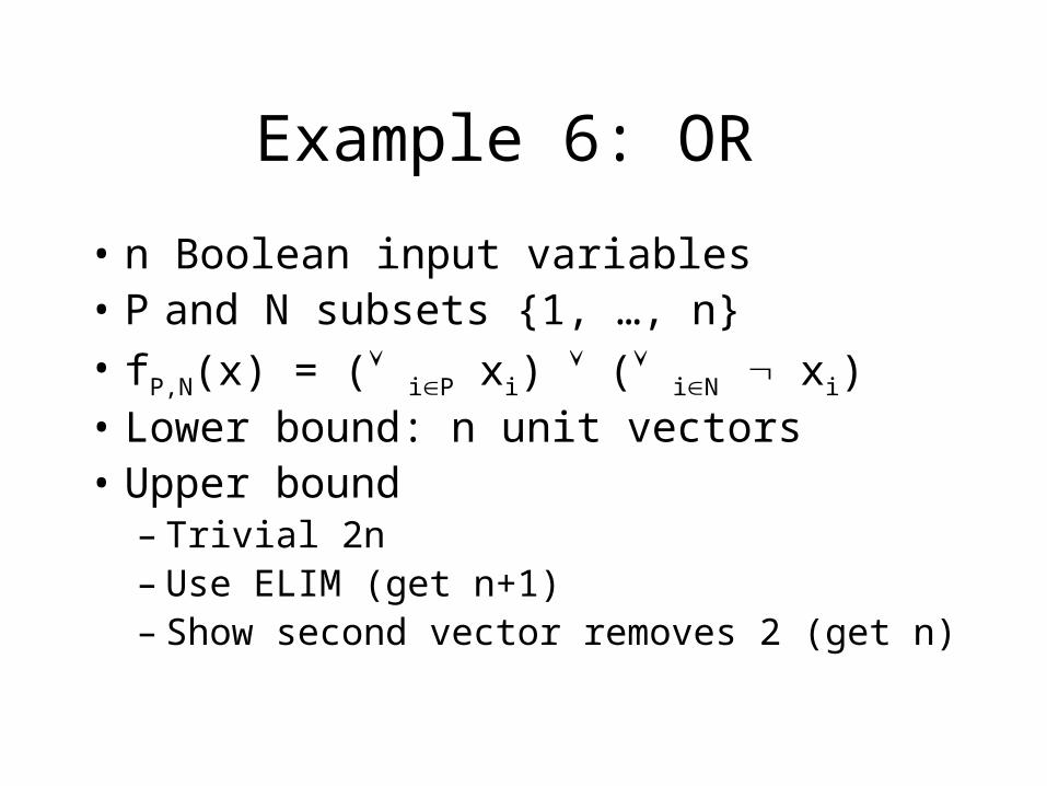
Example 6: OR

• n Boolean input variables• P and N subsets {1, …, n}• fP,N(x) = ( iP xi) ( iN xi)• Lower bound: n unit vectors• Upper bound

– Trivial 2n– Use ELIM (get n+1)– Show second vector removes 2 (get n)

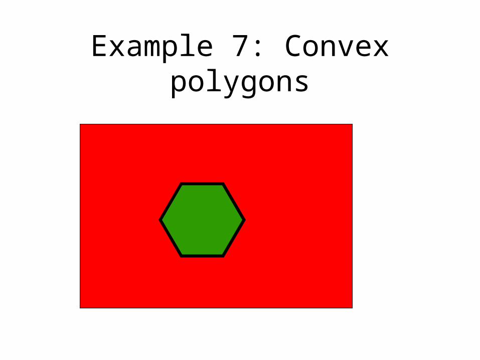
Example 7: Convex polygons

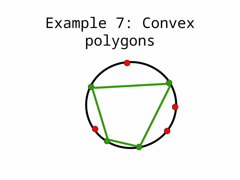
Example 7: Convex polygons

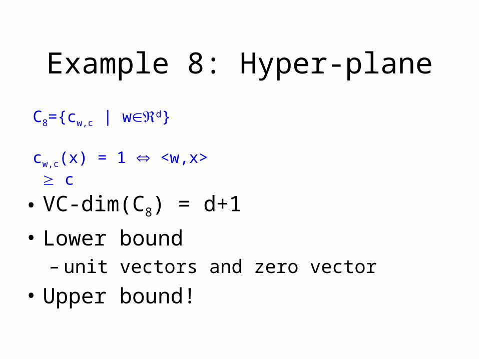
Example 8: Hyper-plane

• VC-dim(C8) = d+1

• Lower bound– unit vectors and zero vector

• Upper bound!

C8={cw,c | wd}

cw,c(x) = 1 <w,x> c

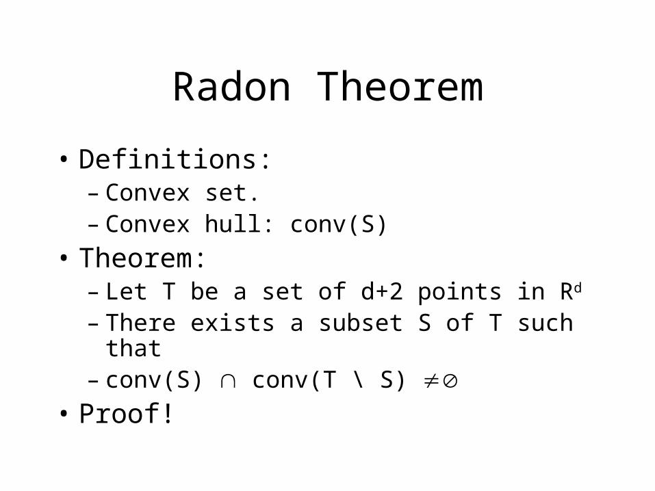
Radon Theorem

• Definitions:– Convex set.– Convex hull: conv(S)

• Theorem:– Let T be a set of d+2 points in Rd

– There exists a subset S of T such that– conv(S) conv(T \ S)

• Proof!

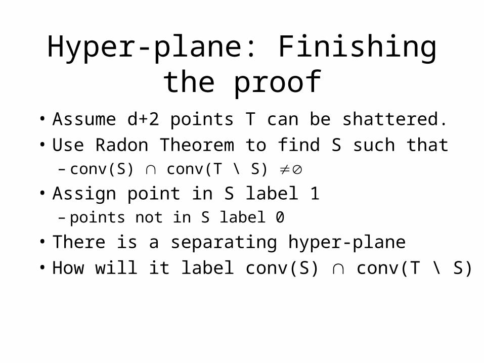
Hyper-plane: Finishing the proof

• Assume d+2 points T can be shattered.

• Use Radon Theorem to find S such that– conv(S) conv(T \ S)

• Assign point in S label 1– points not in S label 0

• There is a separating hyper-plane

• How will it label conv(S) conv(T \ S)

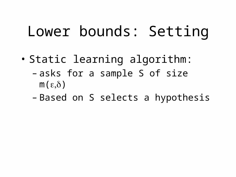
Lower bounds: Setting

• Static learning algorithm:– asks for a sample S of size m()– Based on S selects a hypothesis

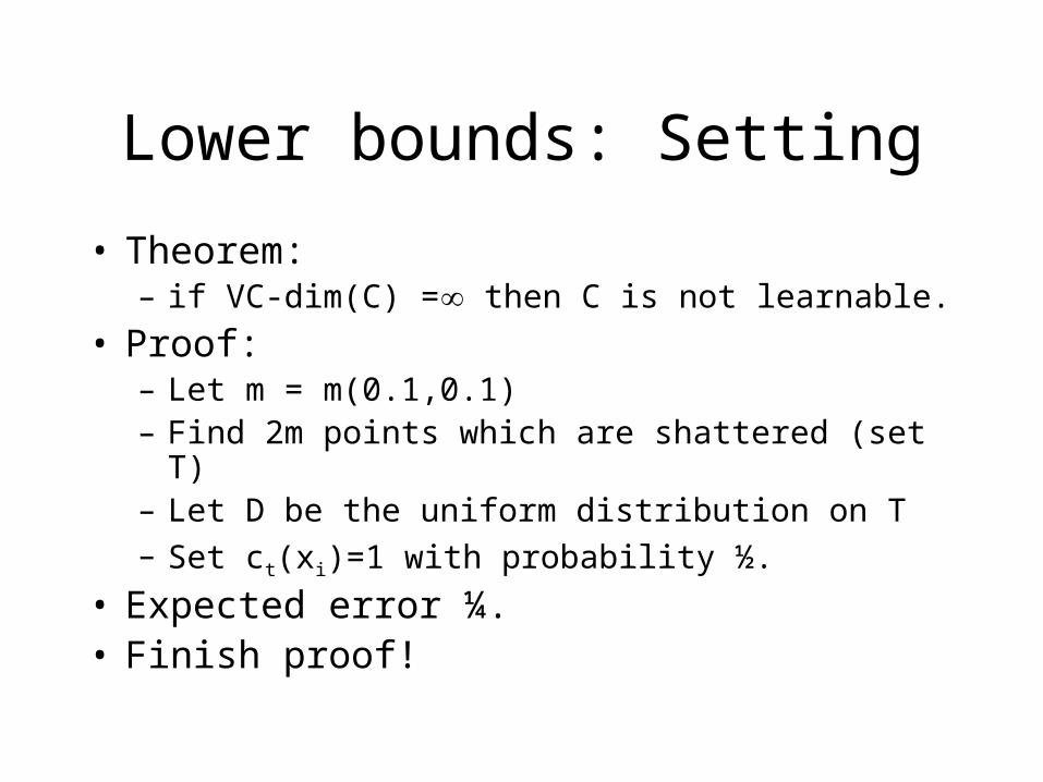
Lower bounds: Setting

• Theorem:– if VC-dim(C) = then C is not learnable.

• Proof:– Let m = m(0.1,0.1)– Find 2m points which are shattered (set T)– Let D be the uniform distribution on T– Set ct(xi)=1 with probability ½.

• Expected error ¼.• Finish proof!

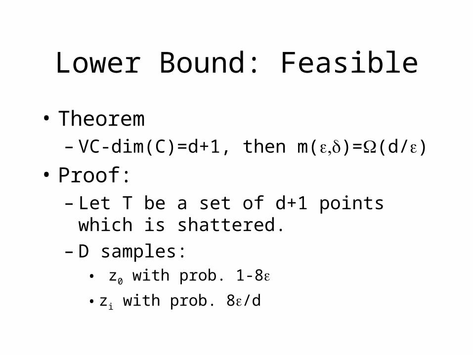
Lower Bound: Feasible

• Theorem– VC-dim(C)=d+1, then m()=(d/)

• Proof:– Let T be a set of d+1 points which is shattered.– D samples:

• z0 with prob. 1-8

• zi with prob. 8/d

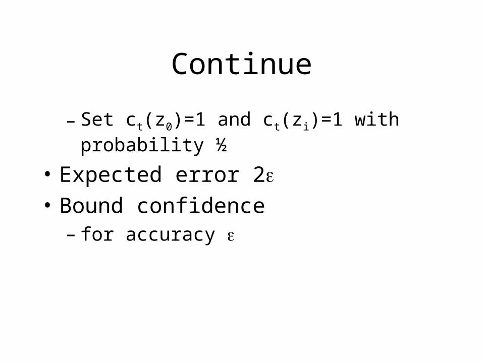
Continue

– Set ct(z0)=1 and ct(zi)=1 with probability ½

• Expected error 2• Bound confidence

– for accuracy

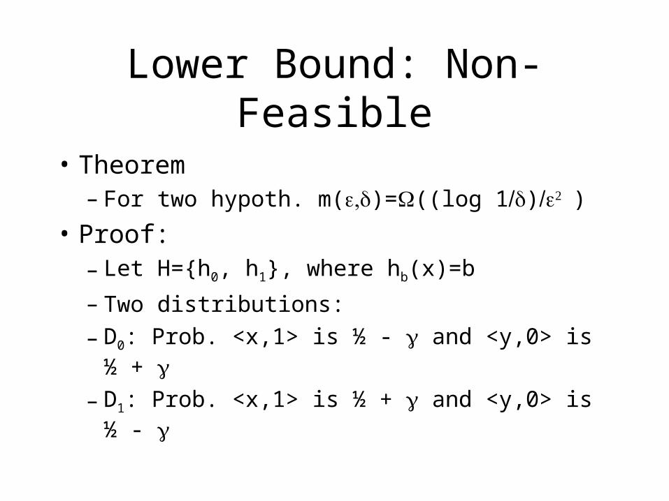
Lower Bound: Non-Feasible

• Theorem– For two hypoth. m()=((log 1))

• Proof:– Let H={h0, h1}, where hb(x)=b

– Two distributions:

– D0: Prob. <x,1> is ½ - and <y,0> is ½ +

– D1: Prob. <x,1> is ½ + and <y,0> is ½ -