Value added in regional climate modeling: Should one attempt improving on the large scales? Lateral boundary condition scheme: Any impact?

Fedor Mesinger 1,2, Katarina Veljović 3, and Borivoj Rajković 3

1) Serbian Academy of Sciences and Arts, Belgrade 2)  Earth System Science Interdisciplinary Center, Un. Maryland, College Park, MD

3)  Institute of Meteorology, Faculty of Physics, Un. of Belgrade, Belgrade

fedor.mesinger@noaa.gov

International Conference on!Planetary Boundary Layers and Climate Change!

Cape Town, South Africa 26-28 October 2009 A plot added, November 18

Update of an earlier conference presentation:

Laprise et al. (Met. Atmos. Ph., 2008) tenets:

• Tenet 1: RCMs are capable of generating small scale features absent in the driving fields supplied as lateral boundary conditions (LBC);

• Tenet 2: The small scales that are generated have the appropriate amplitudes and climate statistics;

• Tenet 3: The generated small scales accurately represent those that would be present in the driving data if it were not limited by resolution;

• Tenet 4: In performing dynamical downscaling, RCM generated small scales are uniquely defined for a given set of LBC.

Laprise et al. “Tenet 5”: • Tenet 5a: The large scales are unaffected within the RCM domain;

• Tenet 5b: The large scales may be improved owing to reduced truncation and explicit treatment of some mesoscale processes with increased resolution within the RCM domain;

• Tenet 5c: The scales larger than or comparable to the RCM domain are degraded because the limited domain is too small to handle these adequately

If you believe in 5c, or if this is “your religion”: “spectral (or, large scale) nudging” inside the domain ! Motivation: “An fundamental assumption in using RCM states that the large-scale atmospheric circulation in the driving data and in the RCM should remain the same at all time” (Lucas-Picher et al., 2004)!

Denis et al. (2002): “the ineffectiveness of the nesting for controlling the large scales over the whole domain”!

Thus, “spectral nudging” (Kida et al., 1991, Waldron et al. 1996; von Storch et al. 2000): provide large scale forcing to the model fields

throughout the entire model domain!

A lot of discussion at:!http://cires.colorado.edu/science/groups/pielke/links/Downscale/!

Castro, C. L., R. A. Pielke, Sr., and G. Leoncini: 2005: Dynamical downscaling: Assessment of value retained and added using the Regional Atmospheric Modeling System (RAMS). J. Geophys. Res., 110, D05108, doi:10.1029/2004JD004721

Castro et al., 4 types of downscaling:

Type 1: NWP (results depends on initial condition); Type 2: “Perfect” LBCs (=reanalysis)

Type 3: GCM (=predicted) LBCs, but still specified SSTs inside Type 4: Fully predicted, both LBCs and inside the RCM domain

*

* In the paper as published, GCM also included within Type 2

Castro, C. L., R. A. Pielke, Sr., and G. Leoncini: 2005: Dynamical downscaling: Assessment of value retained and added using the Regional Atmospheric Modeling System (RAMS). J. Geophys. Res., 110, D05108, doi:10.1029/2004JD004721

Castro et al., 4 types of downscaling:

Type 1: NWP (results depends on initial condition); Type 2: “Perfect” LBCs (=reanalysis)

Type 3: GCM (=predicted) LBCs, but still specified SSTs inside Type 4: Fully predicted, both LBCs and inside the RCM domain

Castro et al.: Type 2, conclusions:

“Absent interior nudging . . . . failure of the RCM to correctly retain value of the large scale . . .”

“. . . underestimation of kinetic energy …” “The results here and past studies suggest the only solution to alleviate this problem is to constrain the RCM with the large-scale model (or reanalysis) values.”

The discussion: 35 very small font pages of e-mails … One e-mail:

Hi Barry

  I do not see how a regional model can reproduce realistic long wave patterns, as these are hemispheric features.

Roger

fm: • We are solving our RCM model equations as an initial-boundary value problem. Doing things inside the domain beyond what RCM equations tell us is in conflict with our basic principles.

Alternative formulation of the same idea: an air parcel inside the RCM knows about forces acting on it, heating it undergoes, etc. It has no allegiance to a given scale !! (It has no idea what goes on on the opposite side of the globe!)

• If the RCM is not doing well the large scales inside the domain, there must be a reason for it;

fm: • We are solving our RCM model equations as an initial-boundary value problem. Doing things inside the domain beyond what RCM equations tell us is in conflict with our basic principles.

Alternative formulation of the same idea: an air parcel inside the RCM knows about forces acting on it, heating it undergoes, etc. It has no allegiance to a given scale !! (It has no idea what goes on on the opposite side of the globe!)

• If the RCM is not doing well the large scales inside the domain, there must be a reason for it;

fm, cont’d: • Type 2 experiments in which reanalysis is declared truth and an RCM’s performance is assessed according to how close to the reanalysis it gets are not appropriate to answer this question. The purpose of an RCM is to improve upon what we have !

Note that in a “thought experiment” a perfect RCM, one that by definition would behave exactly as the real atmosphere, in a Type 2 experiment would depart from reanalysis more and more as the domain gets bigger! (LBCs are not perfect !!)

• There are results claiming or showing improvements in large scales, and at least one Type 3 - albeit somewhat dated - in which improvement in large scales can hardly be questioned !

fm, cont’d: • Type 2 experiments in which reanalysis is declared truth and an RCM’s performance is assessed according to how close to the reanalysis it gets are not appropriate to answer this question. The purpose of an RCM is to improve upon what we have !

Note that in a “thought experiment” a perfect RCM, one that by definition would behave exactly as the real atmosphere, in a Type 2 experiment would depart from reanalysis more and more as the domain gets bigger! (LBCs are not perfect !!)

• There are results claiming or showing improvements in large scales, and at least one Type 3 - albeit somewhat dated - in which improvement in large scales can hardly be questioned !

fm, cont’d: • Type 2 experiments in which reanalysis is declared truth and an RCM’s performance is assessed according to how close to the reanalysis it gets are not appropriate to answer this question. The purpose of an RCM is to improve upon what we have !

Note that in a “thought experiment” a perfect RCM, one that by definition would behave exactly as the real atmosphere, in a Type 2 experiment would depart from reanalysis more and more as the domain gets bigger! (LBCs are not perfect !!)

• There are results claiming or showing improvements in large scales, and at least one Type 3 - albeit somewhat dated - in which improvement in large scales can hardly be questioned !

fm, cont’d: • Type 2 experiments in which reanalysis is declared truth and an RCM’s performance is assessed according to how close to the reanalysis it gets are not appropriate to answer this question. The purpose of an RCM is to improve upon what we have !

Note that in a “thought experiment” a perfect RCM, one that by definition would behave exactly as the real atmosphere, in a Type 2 experiment would depart from reanalysis more and more as the domain gets bigger! (LBCs are not perfect !!)

• There are results claiming or showing improvements in large scales, and at least one Type 3 - albeit somewhat dated - in which improvement in large scales can hardly be questioned !

Giorgi et al., Climatic Change, 1998, 40, 457-493; Mitchell, Fennessy, et al., GEWEX News, 2001, No. 1, 3-6; Gustafson and Leung, BAMS 2007

Fennessy and Altshuler,

2002: 9 ensemble

members

precip difference 1993-1988! Obs.:

COLA GCM:

GCM+ Eta:

An earlier 3-member ensemble result published and discussed in Mitchell, K., M. J. Fennessy, E. Rogers, J. Shukla, T. Black, J. Kinter, F. Mesinger, Z. Janjic, and E. Altshuler, 2001: Simulation of North American summertime climate with the NCEP Eta Model nested in the COLA GCM. GEWEX News, 11, No. 1, 3-6 (Available online at http://www.gewex.org/gewex_nwsltr.html)

The last sentence: In the end then, a nested continental model whose complex physics package has evolved over 1–2 decades with an emphasis on performance over land may indeed have some advantage over its parent GCM for seasonal-range predictions (1–6 months lead) of continental anomalies during the weak circulation regime of summer.

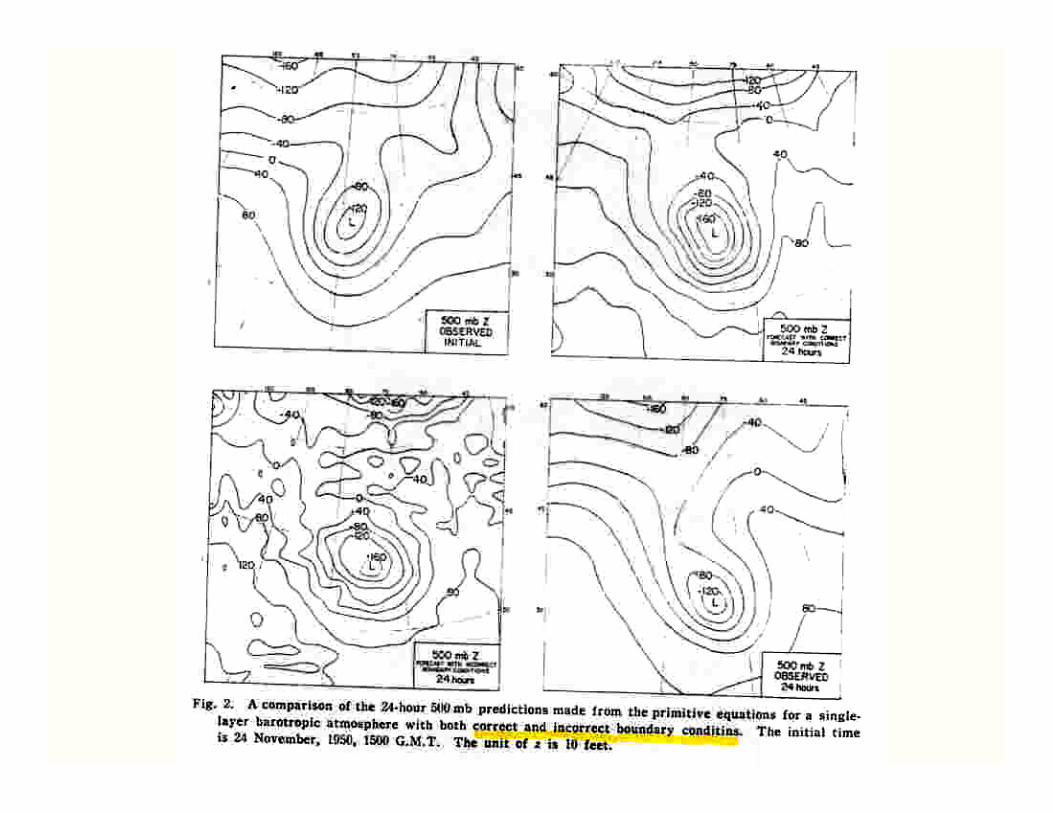
The problem: Considered already in Charney (1962): Linearized shallow-water eqs., one space dimension, characteristics; “at least two conditions have to be specified at inflow points and one condition at outflow”.

• Lateral boundary condition scheme(s)

Subsequently: Sundström (1973)

However:

Davies (1976): “boundary relaxation scheme”

Almost all LA models:

Davies (“relaxation LBCs”):

Outside row: specify all variables

Row 1 grid line inside: specify, e.g., 0.875 * YDM + 0.125 * YLAM Row 2 grid lines inside: 0.750 * YDM + 0.250 * YLAM . . .

Lots of statements published claiming that LBCs are highly detrimental to limited area models !!

(as required by the mathematical nature of the initial-boundary value problem we are solving)

The scheme • At the inflow boundary points, all variables prescribed;

• At the outflow boundary points, tangential velocity extrapolated from the inside (characteristics!);

• The row of grid points next to the boundary row, “buffer row”; variables four-point averaged (this couples

the gravity waves on two C-subgrids of the E-grid)

Thus: No “boundary relaxation” !

Semi-Lagrangian advection the three outermost rows of the integration domain

“limitation”:

Near inflow boundaries, LA model cannot do better - it can only do worse - that its driver model

Thus: have boundaries as far as affordable !

“… the dearth of well-posed meteorological models in the literature is striking.”

(McDonald, MWR 2003)

LBC schemes:

Experiments (work in progress, Veljović, Rajković, Mesinger):

Compare the Eta LBC scheme, against Davies’: use GCM (ECMWF) LBCs and drive the Eta using one and the

other, look at the difference;

Main objective though:

Can one/ does the Eta RCM “retain value of the large scale”? (Castro, Pielke and Leoncini, JGR 2005),

or, more ambitiously,

can one improve on the large scale ?

The Eta code used: “Upgraded (community ?)” Eta

Changes compared to the latest NCEP codes:

• Sloping steps (simplified shaved cells); • Piecewise-linear vertical advection of dynamic variables

(removes a problem of false advection from below ground with the standard Eta Lorenz-Arakawa finite difference scheme)

• Two problems with the lowest layer winds and steps identified and removed;

• Convection scheme parameters; • . . .

LBC experiments:

How can we identify “the skill in large

scales”?

Standard method: “Direct-Cosine

Transform” (DCT, Denis et al. 2002)

How can we identify “the skill in large

scales”?

Standard method: “Direct-Cosine

Transform” (DCT, Denis et al. 2002)

Veljović et al. instead: verification of the

placement of the area of wind speeds > a

chosen large value (50 m/s, later 45 m/s)

Precipitation verification : O

H a

bc

d

F

F : forecast, H : correctly

forecast: “hits” O : observed

“Bias adjusted ETS”: Replace H by Ha :

shows accuracy in placing the event

Equitable threat score (ETS):

€

ETS =H − E(H)

O+ F −H − E(H)

“dHdA method”

(Mesinger 2008): O

H a

bc

d

F

A=F-H : False alarms; Assume as F is increased by dF, ratio of the

infinitesimal increase in H, dH, and that in false alarms dA=dF-dH, is proportional to the yet

unhit area:

F : forecast, H : correctly

forecast: “hits” O : observed

€

b = const

One obtains

( Lambertw, or ProductLog in Mathematica, is the inverse function of

€

z = wew ) €

H(F) =O− 1blambertw bOeb(O−F )( )

€

dHdA

= b(O−H)(dA=dF-dH)

H(F)

H = O

H = F

Fb , Hb

20 40 60 80 100 120 140F

20

40

60

80

100

120H

dHdA method

Results

• Experiments in progress, now using the ECMWF 32 day ensemble, initialized 0000 UTC 1 January 2009;

control T399 (~50 km) / 62 L

Resolution: 31 km/45 layer

Domain size ?

Many people: things get worse as the domain size gets bigger

Reason: reanalysis used to prescribe the LBCs, and reanalysis used as truth ! (Internal variability !)

Assumption: Improving on large scales is possible. However: One cannot improve on large scales if the domain

size is small !

Why is this important?

Domain size ?

Many people: things get worse as the domain size gets bigger

Reason: reanalysis used to prescribe the LBCs, and reanalysis used as truth ! (Internal variability !)

Assumption: Improving on large scales is possible. However: One cannot improve on large scales if the domain

size is small !

Why is this important?

A small gain in large scales is likely to result in large gains in small scales !! :-)

41  

The largest domain of the 10-day experiments (16,400 x 6,000 km):

42  

bias adjusted ETS

Blue : Eta scheme Green : relaxation scheme Red : ECMWF fcst

The largest domain of the 10-day experiments (16,400 x 6,000 km):

43  

bias adjusted ETS

Blue: Eta LBC scheme Green: relaxation scheme Red: ECMWF forecast

44  

bias adjusted ETS

Two LBC schemes:

Eta scheme vs Davies relaxation scheme

No benefit from relaxation

Blue : Eta scheme Green : relaxation scheme Red : ECMWF fcst

The largest domain of the 10-day experiments (16,400 x 6,000 km):

45  

bias adjusted ETS

Bias

Two LBC schemes:

Eta scheme vs Davies relaxation scheme

No benefit from relaxation

Blue : Eta scheme Green : relaxation scheme Red : ECMWF fcst

The largest domain of the 10-day experiments (16,400 x 6,000 km):

46  

bias adjusted ETS

Bias

Two LBC schemes:

Eta scheme vs Davies relaxation scheme

No benefit from relaxation

Placement and area of wind speeds > 50 m/s at 10 days about the same;

No loss of “value of the large scale”

Blue : Eta scheme Green : relaxation scheme Red : ECMWF fcst

The largest domain of the 10-day experiments (16,400 x 6,000 km):

More recent experiments, in progress:

Driver forecasts: ECMWF 32-day ensemble forecast members

T399 (~50 km)/62 level out to 15 days, with 6 h output; lower resolution later

Eta RCM: 31 km/45 layer, 12,000 x 7,580 km domain

Verification against ECMWF analyses

32 day experiments: ECMWF 32 day ensemble: ensemble control + 25 ensemble members

(T399, ~50 km; 62 levels, out to 15 days, reduced resolution later)

The domain:

(12,000 x 7,550 km)

What speeds should we look at ?

> 30 m/s > 45 m/s

What should one do to assess the skill of an ensemble of forecasts ?

Same as what is done with precipitation: add all of the values of H, F, and O

26 (25 members + control) 32-day forecasts:

More traditional verification: root mean square 250 mb wind errors:

All 26 forecasts:

Green: analyses

Black: forecasts

Green: analyses

Black: forecasts

Thus, take home message:

• No disadvantage from using the Eta LBCs (less resource demanding, less of a constraint) compared to relaxation;

• Running the Eta as an RCM, no significant loss of large-scale kinetic energy with time (?);

• The Eta RCM skill in forecasting large scales (with no interior nudging) just about the same as that of the driver model; frequently even higher !!!!!

• This despite the driver global forecast enjoying a bit of an advantage, since it is done using the same model as that which is a part of the data assimilation system !

Thus, take home message:

• No disadvantage from using the Eta LBCs (less resource demanding, less of a constraint) compared to relaxation;

• Running the Eta as an RCM, no significant loss of large-scale kinetic energy with time;

• The Eta RCM skill in forecasting large scales (with no interior nudging) just about the same as that of the driver model; frequently even higher !!!!!

• This despite the driver global forecast enjoying a bit of an advantage, since it is done using the same model as that which is a part of the data assimilation system !

Thus, take home message:

• No disadvantage from using the Eta LBCs (less resource demanding, less of a constraint) compared to relaxation;

• Running the Eta as an RCM, no significant loss of large-scale kinetic energy with time;

• The Eta RCM skill in forecasting large scales (with no interior nudging) just about the same as that of the driver model; frequently even higher !!!!!

• This despite the driver global forecast enjoying a bit of an advantage, since it is done using the same model as that which is a part of the data assimilation system !

Thus, take home message:

• No disadvantage from using the Eta LBCs (less resource demanding, less of a constraint) compared to relaxation;

• Running the Eta as an RCM, no significant loss of large-scale kinetic energy with time;

• The Eta RCM skill in forecasting large scales (with no interior nudging) just about the same as that of the driver model; frequently even higher !!!!!

• This despite the driver global forecast enjoying a bit of an advantage, since it is done using the same model as that which is a part of the data assimilation system !

Thus, take home message:

• No disadvantage from using the Eta LBCs (less resource demanding, less of a constraint) compared to relaxation;

• Running the Eta as an RCM, no significant loss of large-scale kinetic energy with time;

• The Eta RCM skill in forecasting large scales (with no interior nudging) just about the same as that of the driver model; frequently even higher !!!!!

• This despite the driver global forecast enjoying a bit of an advantage, since it is done using the same model as that which is a part of the data assimilation system !

What is/are the main advantage/ main advantages of the Eta making this

happen?

How is that possible ?

Some references (most other available in Giorgi 2006, and/or Laprise et al. 2008)

Laprise, R., R. de Elía, D. Caya, S. Biner, P. Lucas-Picher, E. Diaconescu, M. Leduc, A. Alexandru, and L. Separovic, 2008: Challenging some tenets of Regional Climate Modelling. Meteor. Atmos. Phys., 100, 3-22.!

Lucas-Picher, P., D. Caya, and S. Biner, 2004: RCM’s internal variability as a function of domain size. Res. Activities Atmos. Oceanic Modelling, WMO, Geneva, CAS/JSC WGNE Rep. 34, 7.27-7.28.!

Mesinger, F., 1977: Forward-backward scheme, and its use in a limited area model. Contrib. Atmos. Phys., 50, 200-210.!

Mesinger, F., 2008: Bias adjusted precipitation threat scores. Adv. Geosciences, 16, 137-143. [Available online at http://www.adv-geosci.net/16/index.html.]!

Rockel B., C. L. Castro, R. A. Pielke Sr., H. von Storch, G. Leoncini, 2008: Dynamical downscaling: Assessment of model system dependent retained and added variability for two different regional climate models, J. Geophys. Res., 113, D21107, doi:10.1029/2007JD009461.!

Sundström, A., 1973: Theoretical and practical problems in formulating boundary conditions for a limited area model. Rep. DM-9, Inst. Meteorology, Univ. Stockholm.!

Waldron, K. M., J. Paegle, and J. D. Horel, 1996: Sensitivity of a spectrally filtered and nudged limited-area model to outer model options. Mon. Wea. Rev., 124, 529-547.!

Charney, J. 1962: Integration of the primitive and balance equations. Proc. Intern. Symp. Numerical Weather Prediction, Tokyo, Japan Meteor. Agency, 131-152.!

Davies, H. C., 1976: A lateral boundary formulation for multi-level prediction models. Quart. J. Roy. Meteor. Soc., 102, 405-418.!

Dickinson, R. E., R. M. Errico, F. Giorgi, and G. T. Bates, 1989: A regional climate model for the western United States. Climatic Change, 15, 383-422.!

Fennessy, M. J., and E. L. Altshuler, 2002: Seasonal Climate Predictability in an AGCM and a Nested Regional Model. American Geophysical Union, Fall Meeting 2002, abstract #A61E-06 [Available online at http://adsabs.harvard.edu/abs/2002AGUFM.A61E..06F]!

Giorgi, F., 2006: Regional climate modeling: Status and perspectives. J. Phys. IV France, 139, 101–118, DOI: 10.1051/jp4:2006139008 [Available online at http://jp4.journaldephysique.org/]!

Giorgi, F., and G. T. Bates, 1989: The climatological skill of a regional climate model over complex terrain. Mon. Wea. Rev., 117, 2325–2347.!