VALIDATION OF POWER SYSTEM TRANSIENT STABILITY … · as PSSE, DIgSILENT, EUROSTAG and Matlab’s...
66
VALIDATION OF POWER SYSTEM TRANSIENT STABILITY RESULTS BY KOMAL SUDHIR SHETYE THESIS Submitted in partial fulfillment of the requirements for the degree of Master of Science in Electrical and Computer Engineering in the Graduate College of the University of Illinois at Urbana-Champaign, 2011 Urbana, Illinois Adviser: Professor Thomas J. Overbye
Transcript of VALIDATION OF POWER SYSTEM TRANSIENT STABILITY … · as PSSE, DIgSILENT, EUROSTAG and Matlab’s...
VALIDATION OF POWER SYSTEM TRANSIENT STABILITY RESULTS
BY
KOMAL SUDHIR SHETYE
THESIS
Submitted in partial fulfillment of the requirements for the degree of Master of Science in Electrical and Computer Engineering
in the Graduate College of the University of Illinois at Urbana-Champaign, 2011
Urbana, Illinois
Adviser: Professor Thomas J. Overbye

ii
Abstract
Simulation of the transient stability problem of a power system, which is the assessment
of the short term angular and voltage stability of the system following a disturbance, is of
vital importance. It is widely known in the industry that different transient stability
packages can give substantially different results for the same (or at least similar) system
models. The goal of this work is to develop validation methodologies for different
transient stability software packages with a focus on Western Electricity Coordinating
Council (WECC) system models. We discuss two specific approaches developed and
implemented to validate the transient stability results. The sources of discrepancies seen
in the results from different packages are investigated. This enables us to identify the
differences in the implementation of dynamic models in different transient stability
softwares. In this process, we present certain key analyses of the WECC system models
for different contingencies.

iii
Dedicated with loving memory to my father, Sudhir L. Shetye (1949-2011)

iv
Acknowledgments
I am deeply thankful to my adviser, Professor Thomas Overbye, for his kindness,
guidance, support, significant contributions to this work and his immense patience with
the time it took me to complete this thesis.
This thesis is based on the Power System Engineering Research Center (PSERC) project
entitled “Validation and Accreditation of Transient Stability Results” (Project S43-G). I
am grateful to PSERC’s industry member, the Bonneville Power Administration (BPA),
for funding this work. I thank Jim Gronquist from BPA for providing valuable support
and guidance in this research. I would also like to thank PowerWorld Corporation and
GE for all the technical support provided in this work.
I express deep gratitude towards my parents, especially my father who always inspired
me to pursue excellence in academics and lead a successful career. I am thankful to my
mother, Shakuntala Shetye, for her all her love and support.
Last but not the least, I would like to thank Jay and Ruchika, who have been like my
family in Urbana and who have played a major role in helping me reach this milestone.
v
Table of Contents
1. Introduction ................................................................................................................... 1
2. Detection and Correction of “Bad” Data ...................................................................... 5
3. Validation and Debugging Process: Top-Down Approach .......................................... 9
4. Validation Using Single Machine Infinite Bus Equivalents /
Bottom-Up Approach.................................................................................................. 23
5. Validation of Generator Saturation and Exciter Speed Dependence
Using BPA Data .......................................................................................................... 44
6. Time Step Comparisons .............................................................................................. 49
7. Frequency Comparisons of WECC Case 4 ................................................................. 53
8. Summary and Directions for Future Work ................................................................. 60
References ......................................................................................................................... 61
1
1. Introduction
1.1 Motivation and Problem Overview
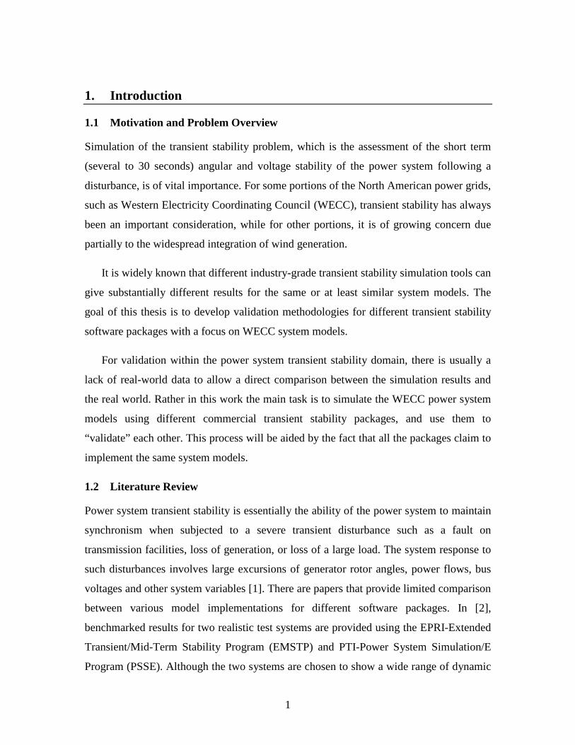
Simulation of the transient stability problem, which is the assessment of the short term
(several to 30 seconds) angular and voltage stability of the power system following a
disturbance, is of vital importance. For some portions of the North American power grids,
such as Western Electricity Coordinating Council (WECC), transient stability has always
been an important consideration, while for other portions, it is of growing concern due
partially to the widespread integration of wind generation.
It is widely known that different industry-grade transient stability simulation tools can
give substantially different results for the same or at least similar system models. The
goal of this thesis is to develop validation methodologies for different transient stability
software packages with a focus on WECC system models.
For validation within the power system transient stability domain, there is usually a
lack of real-world data to allow a direct comparison between the simulation results and
the real world. Rather in this work the main task is to simulate the WECC power system
models using different commercial transient stability packages, and use them to
“validate” each other. This process will be aided by the fact that all the packages claim to
implement the same system models.
1.2 Literature Review
Power system transient stability is essentially the ability of the power system to maintain
synchronism when subjected to a severe transient disturbance such as a fault on
transmission facilities, loss of generation, or loss of a large load. The system response to
such disturbances involves large excursions of generator rotor angles, power flows, bus
voltages and other system variables [1]. There are papers that provide limited comparison
between various model implementations for different software packages. In [2],
benchmarked results for two realistic test systems are provided using the EPRI-Extended
Transient/Mid-Term Stability Program (EMSTP) and PTI-Power System Simulation/E
Program (PSSE). Although the two systems are chosen to show a wide range of dynamic

2
characteristics in terms of the mode of instability, they include only two types of machine
models, namely the classical model and the two axis model with exciters. The actual
number of the types of these models in the WECC system is far more. In [3], the authors
evaluate more transient stability software packages such as DIgSILENT, PSSE, and
PSCAD on the basis of the power system component models available in each tool and
their user-friendliness. However, only a limited number of component models such as
synchronous generator, generator saturation, transmission line representation and external
network are compared and only one simplified test case is used. K. K. Kabere et al.
investigate the turbo-generator modeling employed by five industrial-grade power system
simulation tools (PSSE, PowerFactory, EUROSTAG, SSAT and MatNetEig) in their
application for small-signal stability analysis [4]. From the disparities in the results
obtained from simulating the same system in different tools, the authors conclude that
validation of results obtained from different small-signal analysis tools with field
experiments is crucial, as is the necessity of benchmarking and standardization of
requirements for different simulation tools. In [5], validation of different softwares such
as PSSE, DIgSILENT, EUROSTAG and Matlab’s Power System Toolbox (PST) was
performed with a focus on small-signal stability. Again, here the focus was on generator
modeling and solution methodologies. In [6], steady-state performance and the impact of
a three-phase transient disturbance were used as the basis for comparisons between some
softwares that allow HVDC lines to be modeled, namely DigSILENT, Matlab PST and
PSAT. An important conclusion drawn from this work was that the steady state analysis
results were similar, especially for the more established and widely used packages like
PSSE and DigSILENT. Even in the packages that we are considering in our work such as
PowerWorld Simulator, PSSE and GE’s Positive Sequence Load Flow program (PSLF),
owing to their long history of use of power flow analysis, we expected and correctly
encountered a good agreement between the packages with respect to their static network
solutions. Since the initialization of a transient stability simulation is based on the steady
state network solution, this key fact enabled us to validate our transient stability results
more effectively, and any discrepancies in the results from these comparisons could thus
be attributed majorly to the dynamic simulation solution.

3
There are a number of industry and IEEE approved generator, exciter, stabilizer,
governor, load and other models that are used in transient stability studies. Some of these
models have slightly different representations in different transient stability software
packages [7], [8], [9]. This work focuses only on the models used most commonly in the
WECC system. Reference [7] contains an extensive library of such models used
commonly in industry, a subset of which was analyzed in this work.
1.3 Related Project
This thesis is based on a project funded by the Bonneville Power Administration (BPA),
which falls under the purview of WECC. This work was conducted through the Power
Systems Engineering Research Center (PSERC). The goal of this project was to enhance
the utilization of the BPA transmission system by using validated, real-time transient
stability analysis results, and to have better planning/study tools and models. We also
provided benchmarked cases and results to BPA to aid their simulation studies on their
interconnected power system. This thesis describes the validation studies performed
using PowerWorld, PSSE and PSLF. In this project, we received three different versions
of the complete WECC power system model comprising roughly 17,000 buses and 3000
generators in PSLF format, and one in the PSSE format. Each successive PSLF case was
an improved and updated one. We converted these files to PowerWorld binary files
(*.pwb) for the ease of our studies across different packages. In this thesis, we will refer
to the case files by the following names:
1. WECC Case 1: PSLF format
2. WECC Case 2: PSLF format
This updated case, received on June 28 2010, fixed some 2000 errors in the
previous version
3. WECC Case 3: PSSE format
This was the only WECC case received in the PSSE format, in December 2010.

4
4. WECC Case 4: PSLF format
This was the most recent and updated case provided to us.
Following the WECC standard, a time step of ¼ cycle was used in all the simulations,
unless specified otherwise.
The single machine infinite bus (SMIB) cases analyzed in this work were derived
from specific buses from the full WECC model. The generator buses from which these
equivalents were derived are mentioned in this thesis.
In order to ensure confidentiality of the WECC system data, alternative bus numbers,
area names, etc., have been assigned in this thesis, which do not reflect, in any way, the
actual numbers or names of any part of the system. This is also the reason why we have
maintained ambiguity about locations and names of components such as generating units.
1.4 Thesis Organization
The organization of the thesis is as follows. Chapter 2 describes the detection and
correction of bad dynamic model data that we encountered in the full WECC model, and
the principles of time-step and auto-correction. Chapter 3 charts out the first aspect of our
validation methodology, i.e. the top-down approach, and eventually highlights the
significance of SMIB equivalents in the debugging process. Chapter 4 covers the bottom-
up approach to validation in some detail, wherein we use SMIB equivalents to validate
the major generator models. Chapter 5 discusses validation of generator saturation and
exciters with results for the full WECC case, provided by BPA. Chapter 6 provides an
insight into time step comparison of results. Chapter 7 describes the latest runs being
done on Case 4, some comparison results and the issues encountered. Lastly, Chapter 8
summarizes this work and gives directions for future research.

5
2. Detection and Correction of “Bad” Data
2.1 Background
The “Run Validation” option in the Transient Stability module of PowerWorld allows the
user to check for any data imperfections prior to running a transient stability simulation.
The “Validation Errors” essentially are a list of parameters that depict non-physical
scenarios or those which might cause the simulation to be numerically unstable or
compromise accuracy. Suggestions for auto-correcting some of these parameters are
made by PowerWorld, when these errors are encountered. Quite a few of such errors
were found in the WECC full cases, which were reported to BPA. Detecting the errors
thus made vast improvements in the WECC model. The following sections throw light on
this detection and correction of “bad” data.
2.2 Correction of Bad Saturation Data
Magnetic saturation affects the various mutual and leakage inductances within a machine,
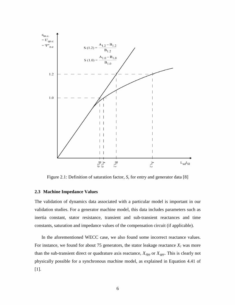
except the classical generator (GENCLS) model [8]. Saturation data for a machine is
entered by specifying the values of two parameters S(1.0) and S(1.2), which are defined
in Figure 2.1. It is a known fact that magnetic material saturates with higher flux.
Therefore the value of S(1.2) can never be less than the value of S(1.0).
For WECC Case 2, the saturation data for about 28 generators failed to meet the
criteria S(1.2) >= S(1.0). This was detected in the PowerWorld validation run.
The suggested auto-correction was to swap the values of S(1.0) with S(1.2).
6
Figure 2.1: Definition of saturation factor, S, for entry and generator data [8]
2.3 Machine Impedance Values
The validation of dynamics data associated with a particular model is important in our
validation studies. For a generator machine model, this data includes parameters such as
inertia constant, stator resistance, transient and sub-transient reactances and time
constants, saturation and impedance values of the compensation circuit (if applicable).
In the aforementioned WECC case, we also found some incorrect reactance values.
For instance, we found for about 75 generators, the stator leakage reactance Xl was more
than the sub-transient direct or quadrature axis reactance, Xdpp or Xqpp. This is clearly not
physically possible for a synchronous machine model, as explained in Equation 4.41 of
[1].

7
2.4 Correction of Time Constants
Setting the appropriate time step is important from the point of view of accuracy and
numerical stability of the simulation. Time step is specified either in seconds or a fraction
of one cycle. The nominal system frequency for the power system used in our study is 60
cycles per second. As recommended by BPA to follow the WECC standard, a time step
of ¼ cycle has been used all throughout this work to conduct all the transient stability
simulations, unless specified otherwise.
From Equations 11.3 to 11.7 of [8], it is clear that the numerical integration process in
a dynamic simulation can be accurate and stable only if the time step ∆t is small in
comparison to the time constants used in the simulation; otherwise the integration process
might develop an error that grows unstably [8].
PSSE uses the second order Euler scheme to perform numerical integration. From the
experience of these transient stability package developers, it is indicated that numerical
instability problems will be avoided and the accuracy will be sufficient if the time step is
kept 1/4 to 1/5 times smaller than the shortest time constant being used in the simulation.
In the validation run, PowerWorld also detected some time constants that were less
than four times the time step ∆t. These were reported as validation errors. The auto-
correction converts these time constants to higher values to meet the criteria with
reference to the time step size.
2.5 Correction of Dynamic Model Parameters
Besides machine model parameters, data errors were also found in the parameters of a
particular governor model namely the 1981 IEEE type 1 turbine-governor model or
commonly known as IEEEG1.
8
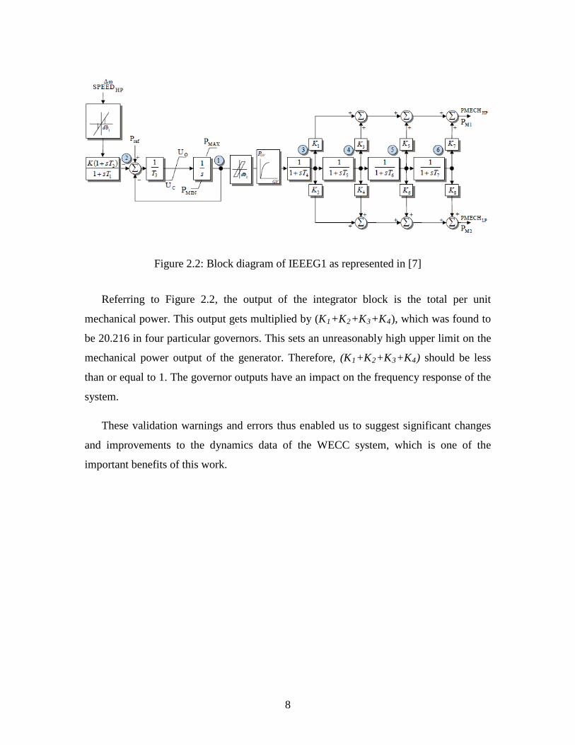
Figure 2.2: Block diagram of IEEEG1 as represented in [7]
Referring to Figure 2.2, the output of the integrator block is the total per unit
mechanical power. This output gets multiplied by (K1+K2+K3+K4), which was found to
be 20.216 in four particular governors. This sets an unreasonably high upper limit on the
mechanical power output of the generator. Therefore, (K1+K2+K3+K4) should be less
than or equal to 1. The governor outputs have an impact on the frequency response of the
system.
These validation warnings and errors thus enabled us to suggest significant changes
and improvements to the dynamics data of the WECC system, which is one of the
important benefits of this work.
9
3. Validation and Debugging Process: Top-Down Approach
This chapter highlights how large case simulations were used to detect potential analysis
software problems. This example uses WECC Case 4. The validation process was
comparing the transient stability runs done in PowerWorld Simulator Version 16 (beta)
with the PSLF Dynamics Susbsystem (PSDS) Version 17 results provided by BPA.
During the simulation the bus frequencies and voltages were monitored at 20 locations
selected by BPA to give a representation of system behavior. For the simulations, the
system was initially allowed to run unperturbed for two seconds to demonstrate a stable
initial contingency. Then at time t = 2.0 seconds, 2 large generating units in the southern
part of the WECC system were dropped and the simulation was run for a total of 30
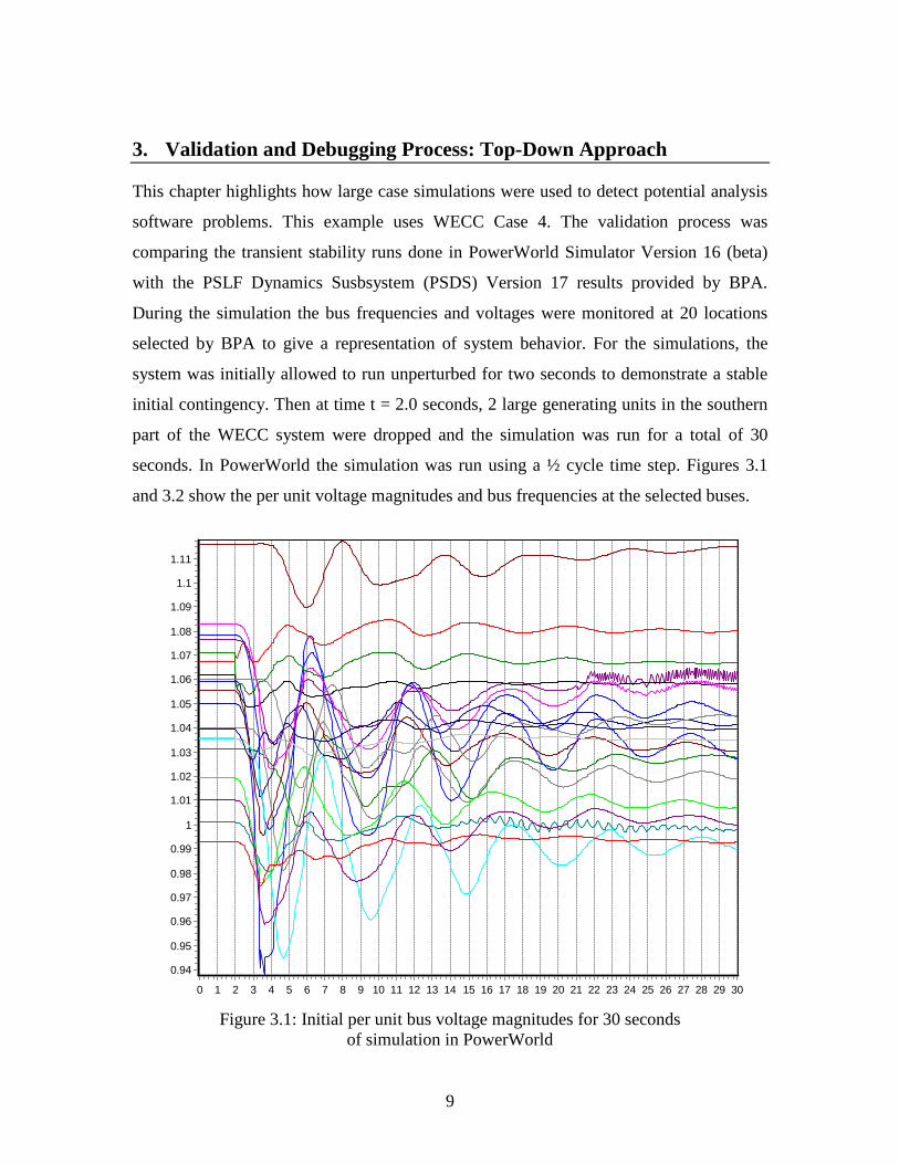
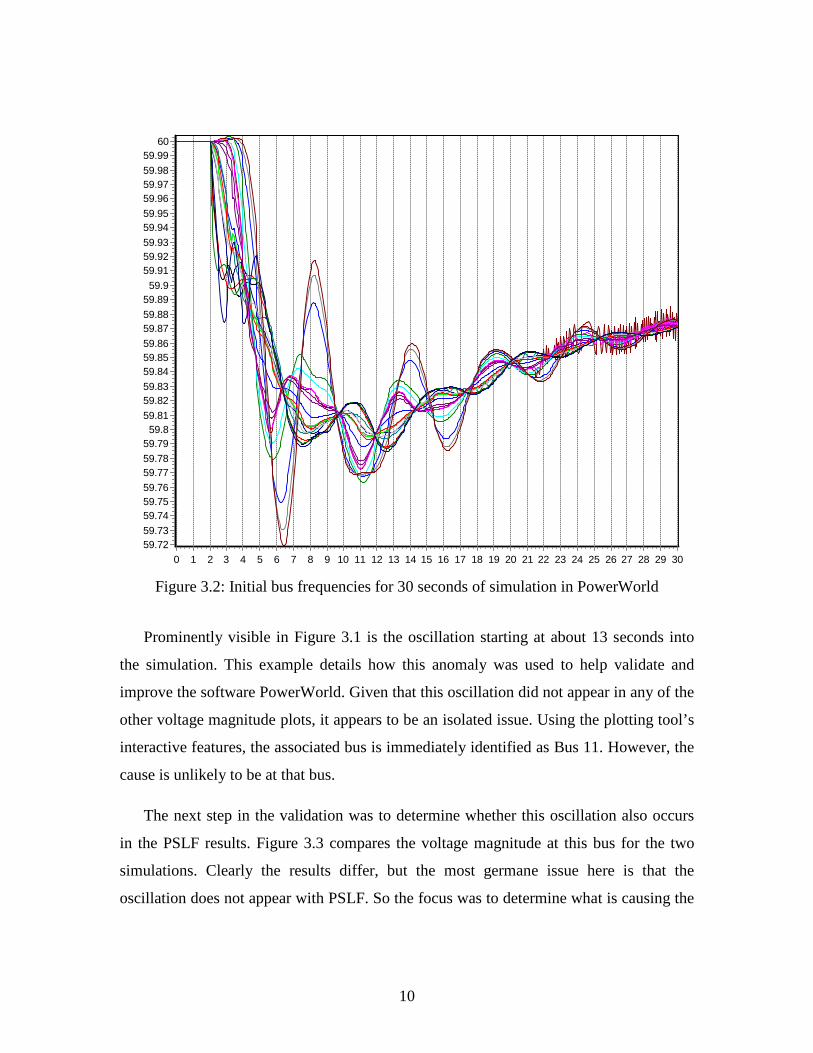
seconds. In PowerWorld the simulation was run using a ½ cycle time step. Figures 3.1
and 3.2 show the per unit voltage magnitudes and bus frequencies at the selected buses.
Figure 3.1: Initial per unit bus voltage magnitudes for 30 seconds
of simulation in PowerWorld
3029282726252423222120191817161514131211109876543210
1.11
1.1
1.09
1.08
1.07
1.06
1.05
1.04
1.03
1.02
1.01
1
0.99
0.98
0.97
0.96
0.95
0.94
10
Figure 3.2: Initial bus frequencies for 30 seconds of simulation in PowerWorld
Prominently visible in Figure 3.1 is the oscillation starting at about 13 seconds into
the simulation. This example details how this anomaly was used to help validate and
improve the software PowerWorld. Given that this oscillation did not appear in any of the
other voltage magnitude plots, it appears to be an isolated issue. Using the plotting tool’s
interactive features, the associated bus is immediately identified as Bus 11. However, the
cause is unlikely to be at that bus.
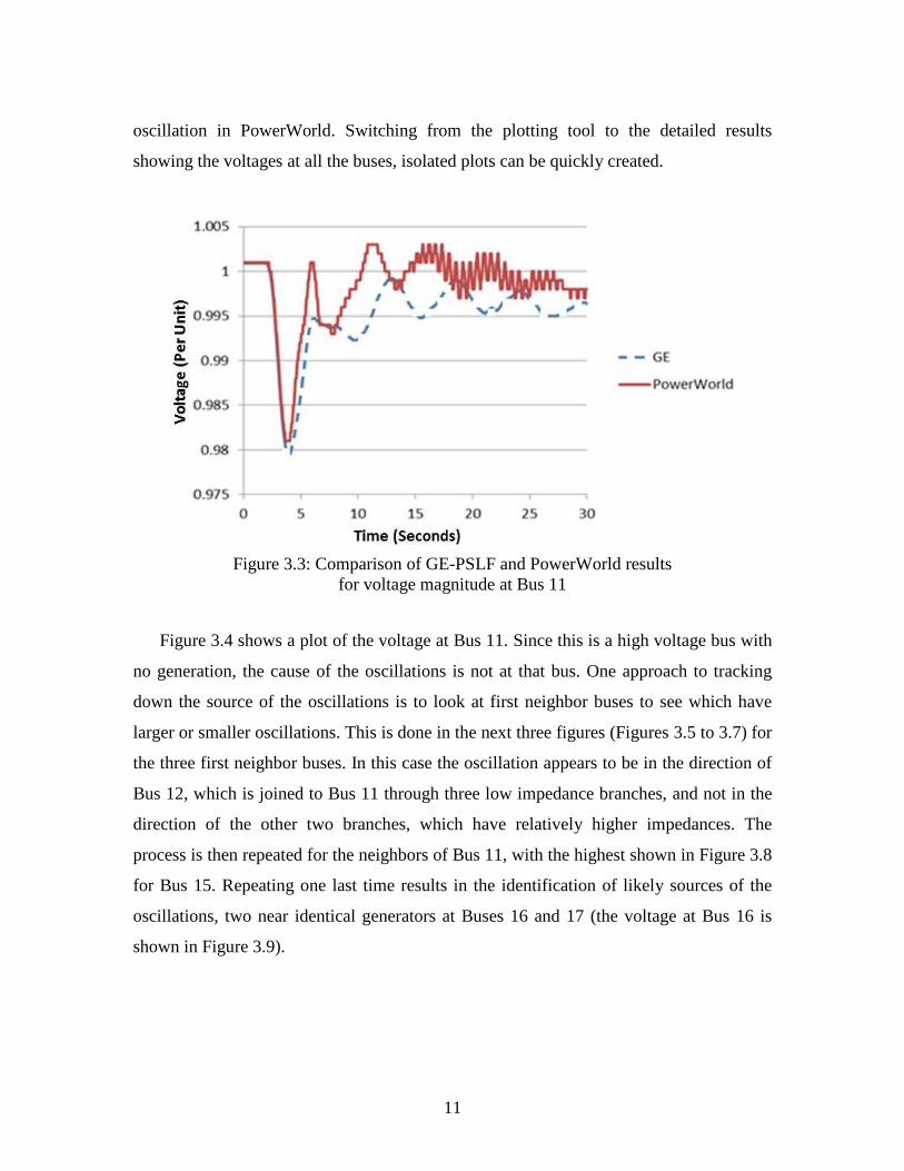
The next step in the validation was to determine whether this oscillation also occurs
in the PSLF results. Figure 3.3 compares the voltage magnitude at this bus for the two
simulations. Clearly the results differ, but the most germane issue here is that the
oscillation does not appear with PSLF. So the focus was to determine what is causing the
3029282726252423222120191817161514131211109876543210
6059.9959.9859.9759.9659.9559.9459.9359.9259.9159.9
59.8959.8859.8759.8659.8559.8459.8359.8259.8159.8
59.7959.7859.7759.7659.7559.7459.7359.72
11
oscillation in PowerWorld. Switching from the plotting tool to the detailed results
showing the voltages at all the buses, isolated plots can be quickly created.
Figure 3.3: Comparison of GE-PSLF and PowerWorld results
for voltage magnitude at Bus 11
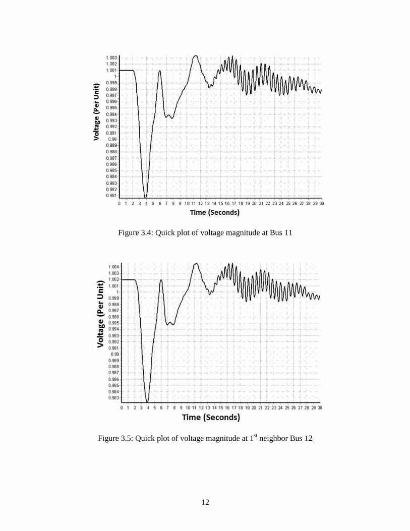
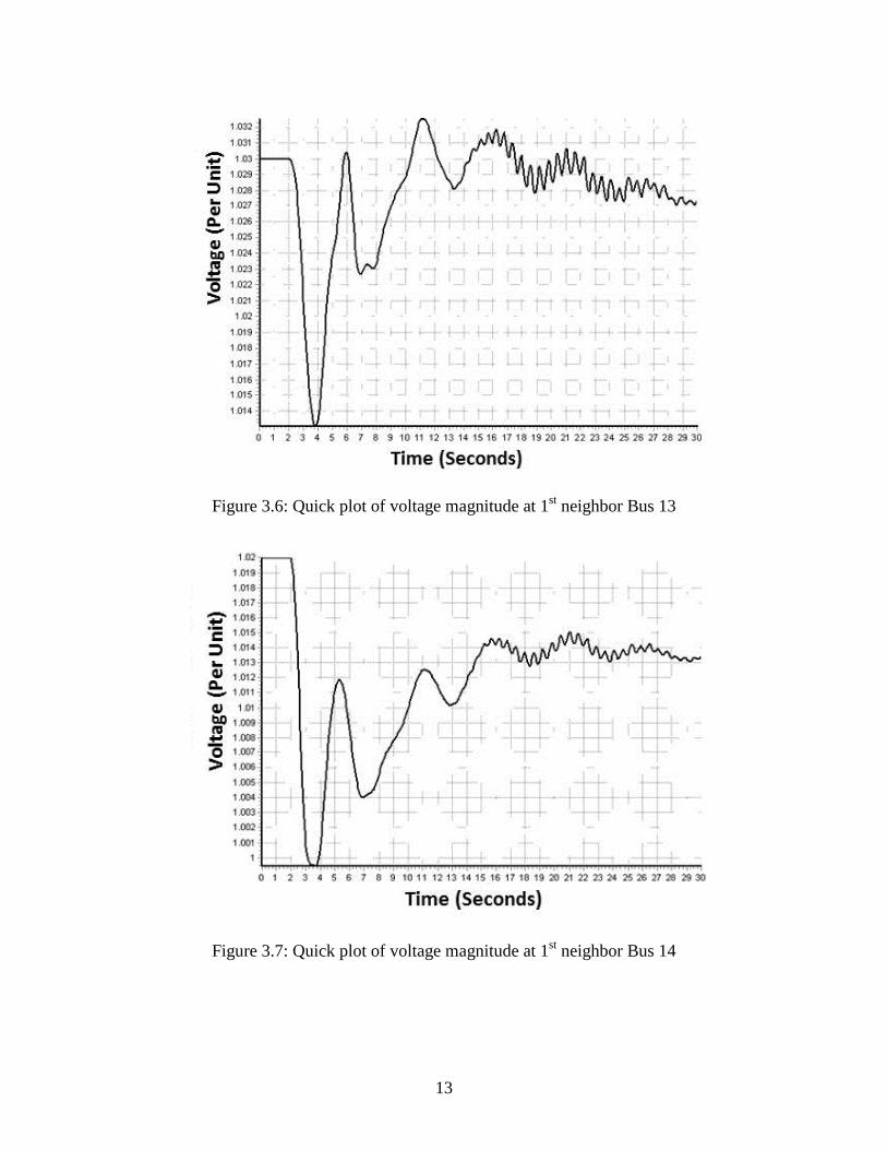
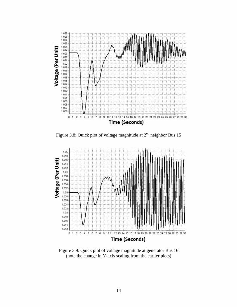
Figure 3.4 shows a plot of the voltage at Bus 11. Since this is a high voltage bus with
no generation, the cause of the oscillations is not at that bus. One approach to tracking
down the source of the oscillations is to look at first neighbor buses to see which have
larger or smaller oscillations. This is done in the next three figures (Figures 3.5 to 3.7) for
the three first neighbor buses. In this case the oscillation appears to be in the direction of
Bus 12, which is joined to Bus 11 through three low impedance branches, and not in the
direction of the other two branches, which have relatively higher impedances. The
process is then repeated for the neighbors of Bus 11, with the highest shown in Figure 3.8
for Bus 15. Repeating one last time results in the identification of likely sources of the
oscillations, two near identical generators at Buses 16 and 17 (the voltage at Bus 16 is
shown in Figure 3.9).
12
Figure 3.4: Quick plot of voltage magnitude at Bus 11
Figure 3.5: Quick plot of voltage magnitude at 1st neighbor Bus 12
13
Figure 3.6: Quick plot of voltage magnitude at 1st neighbor Bus 13
Figure 3.7: Quick plot of voltage magnitude at 1st neighbor Bus 14
14
Figure 3.8: Quick plot of voltage magnitude at 2nd neighbor Bus 15
Figure 3.9: Quick plot of voltage magnitude at generator Bus 16
(note the change in Y-axis scaling from the earlier plots)
15
An alternative process is to utilize the SMIB eigenvalue analysis process to see if
there are any generators with positive eigenvalues in the vicinity of Bus 11. For this
example, this process worked quite quickly since there were only two generators in the
same area as 11 with positive eigenvalues, 16 and 17.
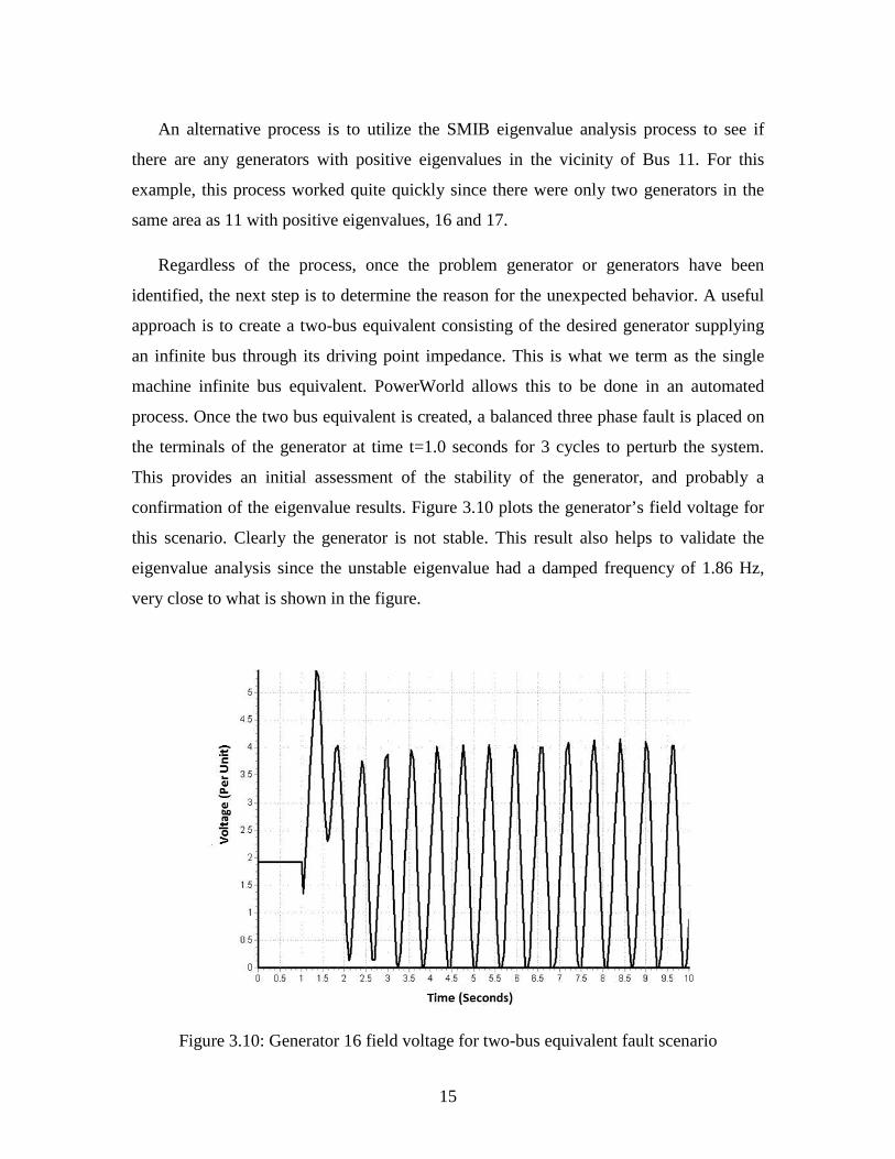
Regardless of the process, once the problem generator or generators have been
identified, the next step is to determine the reason for the unexpected behavior. A useful
approach is to create a two-bus equivalent consisting of the desired generator supplying
an infinite bus through its driving point impedance. This is what we term as the single
machine infinite bus equivalent. PowerWorld allows this to be done in an automated
process. Once the two bus equivalent is created, a balanced three phase fault is placed on
the terminals of the generator at time t=1.0 seconds for 3 cycles to perturb the system.
This provides an initial assessment of the stability of the generator, and probably a
confirmation of the eigenvalue results. Figure 3.10 plots the generator’s field voltage for
this scenario. Clearly the generator is not stable. This result also helps to validate the
eigenvalue analysis since the unstable eigenvalue had a damped frequency of 1.86 Hz,
very close to what is shown in the figure.
Figure 3.10: Generator 16 field voltage for two-bus equivalent fault scenario
16
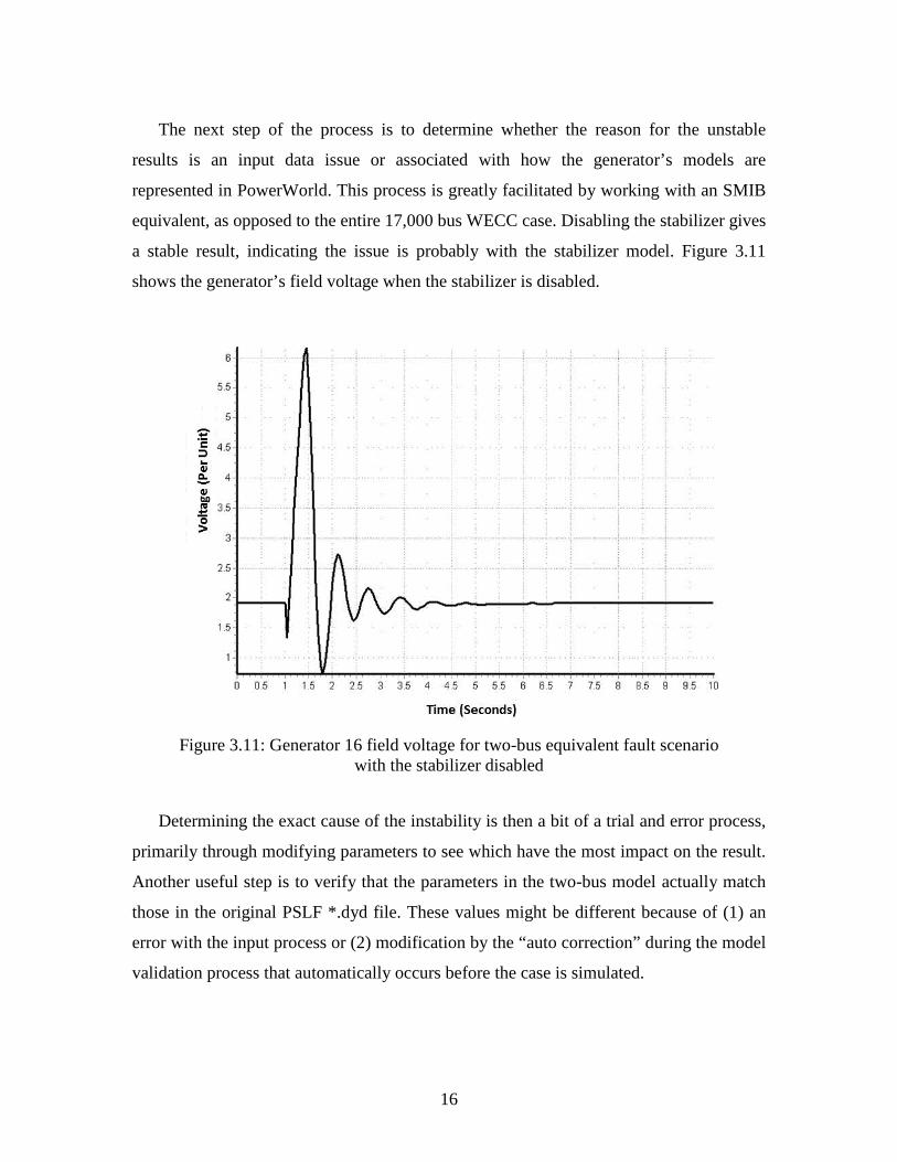
The next step of the process is to determine whether the reason for the unstable
results is an input data issue or associated with how the generator’s models are
represented in PowerWorld. This process is greatly facilitated by working with an SMIB
equivalent, as opposed to the entire 17,000 bus WECC case. Disabling the stabilizer gives
a stable result, indicating the issue is probably with the stabilizer model. Figure 3.11
shows the generator’s field voltage when the stabilizer is disabled.
Figure 3.11: Generator 16 field voltage for two-bus equivalent fault scenario
with the stabilizer disabled
Determining the exact cause of the instability is then a bit of a trial and error process,
primarily through modifying parameters to see which have the most impact on the result.
Another useful step is to verify that the parameters in the two-bus model actually match
those in the original PSLF *.dyd file. These values might be different because of (1) an
error with the input process or (2) modification by the “auto correction” during the model
validation process that automatically occurs before the case is simulated.
17
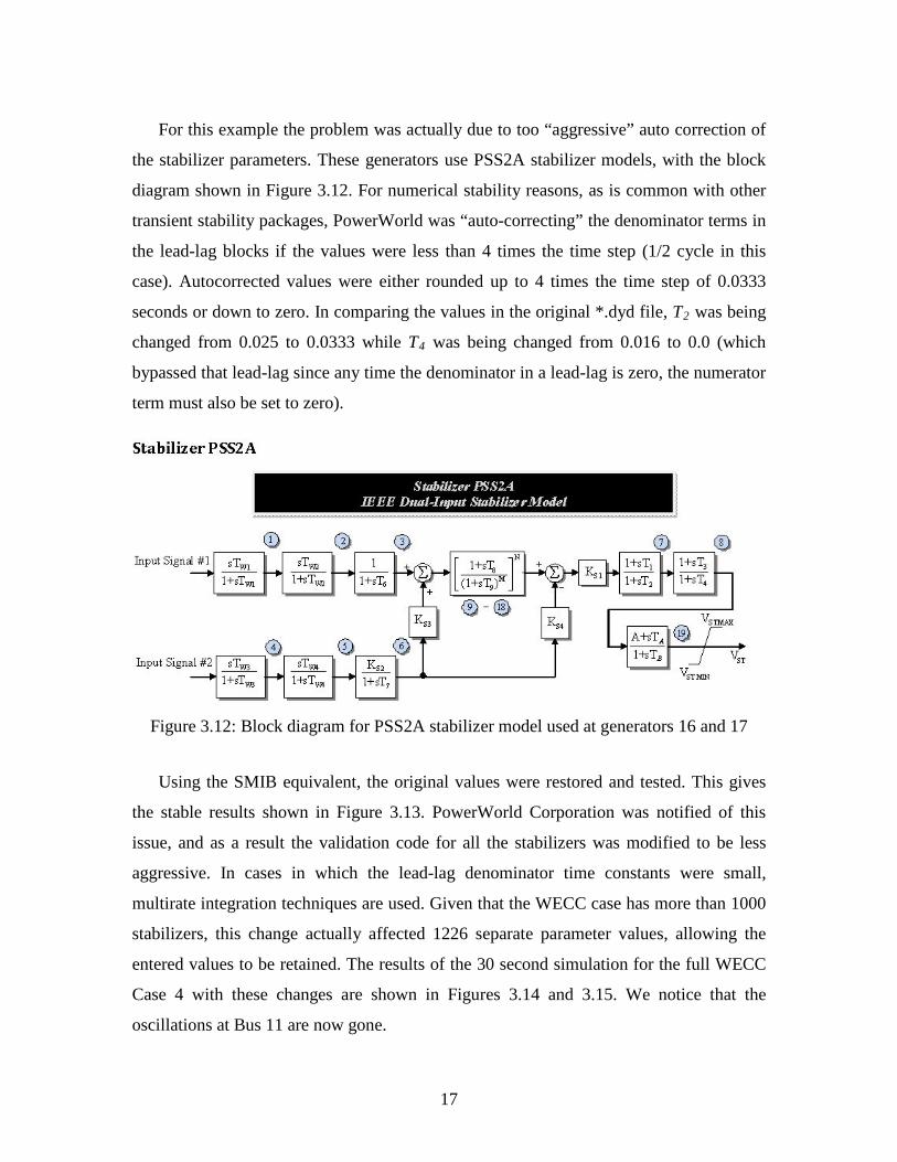
For this example the problem was actually due to too “aggressive” auto correction of
the stabilizer parameters. These generators use PSS2A stabilizer models, with the block
diagram shown in Figure 3.12. For numerical stability reasons, as is common with other
transient stability packages, PowerWorld was “auto-correcting” the denominator terms in
the lead-lag blocks if the values were less than 4 times the time step (1/2 cycle in this
case). Autocorrected values were either rounded up to 4 times the time step of 0.0333
seconds or down to zero. In comparing the values in the original *.dyd file, T2 was being
changed from 0.025 to 0.0333 while T4 was being changed from 0.016 to 0.0 (which
bypassed that lead-lag since any time the denominator in a lead-lag is zero, the numerator
term must also be set to zero).
Figure 3.12: Block diagram for PSS2A stabilizer model used at generators 16 and 17
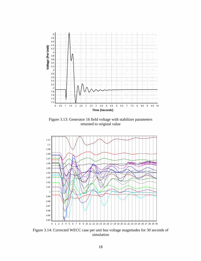
Using the SMIB equivalent, the original values were restored and tested. This gives
the stable results shown in Figure 3.13. PowerWorld Corporation was notified of this
issue, and as a result the validation code for all the stabilizers was modified to be less
aggressive. In cases in which the lead-lag denominator time constants were small,
multirate integration techniques are used. Given that the WECC case has more than 1000
stabilizers, this change actually affected 1226 separate parameter values, allowing the
entered values to be retained. The results of the 30 second simulation for the full WECC
Case 4 with these changes are shown in Figures 3.14 and 3.15. We notice that the
oscillations at Bus 11 are now gone.
18
Figure 3.13: Generator 16 field voltage with stabilizer parameters
returned to original value
Figure 3.14: Corrected WECC case per unit bus voltage magnitudes for 30 seconds of
simulation
3029282726252423222120191817161514131211109876543210
1.11
1.1
1.09
1.08
1.07
1.06
1.05
1.04
1.03
1.02
1.01
1
0.99
0.98
0.97
0.96
0.95
0.94
19
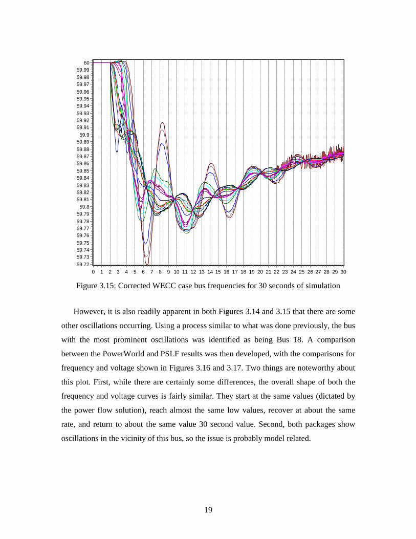
Figure 3.15: Corrected WECC case bus frequencies for 30 seconds of simulation
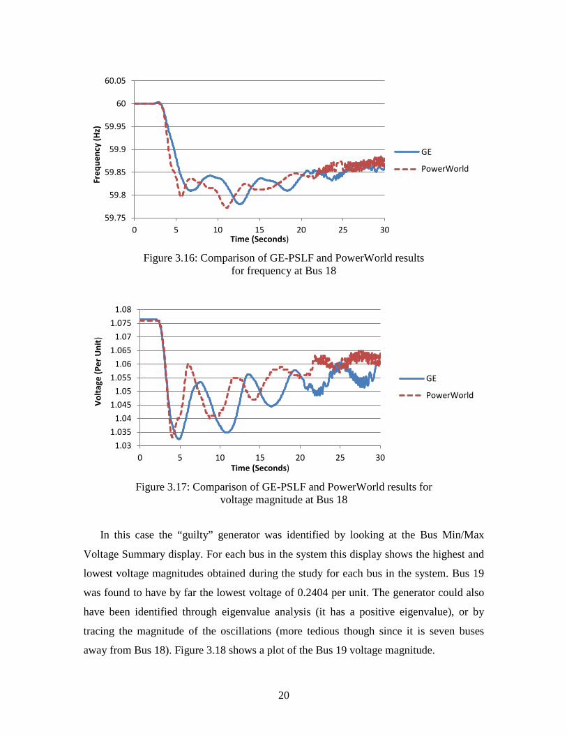
However, it is also readily apparent in both Figures 3.14 and 3.15 that there are some
other oscillations occurring. Using a process similar to what was done previously, the bus
with the most prominent oscillations was identified as being Bus 18. A comparison
between the PowerWorld and PSLF results was then developed, with the comparisons for
frequency and voltage shown in Figures 3.16 and 3.17. Two things are noteworthy about
this plot. First, while there are certainly some differences, the overall shape of both the
frequency and voltage curves is fairly similar. They start at the same values (dictated by
the power flow solution), reach almost the same low values, recover at about the same
rate, and return to about the same value 30 second value. Second, both packages show
oscillations in the vicinity of this bus, so the issue is probably model related.
3029282726252423222120191817161514131211109876543210
6059.9959.9859.9759.9659.9559.9459.9359.9259.91
59.959.8959.8859.8759.8659.8559.8459.8359.8259.81
59.859.7959.7859.7759.7659.7559.7459.7359.72
20
Figure 3.16: Comparison of GE-PSLF and PowerWorld results
for frequency at Bus 18
Figure 3.17: Comparison of GE-PSLF and PowerWorld results for
voltage magnitude at Bus 18
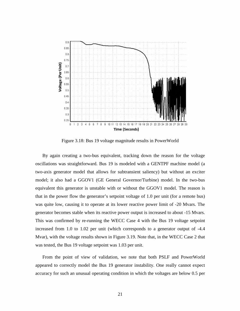
In this case the “guilty” generator was identified by looking at the Bus Min/Max
Voltage Summary display. For each bus in the system this display shows the highest and
lowest voltage magnitudes obtained during the study for each bus in the system. Bus 19
was found to have by far the lowest voltage of 0.2404 per unit. The generator could also
have been identified through eigenvalue analysis (it has a positive eigenvalue), or by
tracing the magnitude of the oscillations (more tedious though since it is seven buses
away from Bus 18). Figure 3.18 shows a plot of the Bus 19 voltage magnitude.
59.75
59.8
59.85
59.9
59.95
60
60.05
0 5 10 15 20 25 30
Freq
uenc
y (H
z)
Time (Seconds)
GE
PowerWorld
1.031.035
1.041.045
1.051.055
1.061.065
1.071.075
1.08
0 5 10 15 20 25 30
Volta
ge (P
er U
nit)
Time (Seconds)
GE
PowerWorld
21
Figure 3.18: Bus 19 voltage magnitude results in PowerWorld
By again creating a two-bus equivalent, tracking down the reason for the voltage
oscillations was straightforward. Bus 19 is modeled with a GENTPF machine model (a
two-axis generator model that allows for subtransient saliency) but without an exciter
model; it also had a GGOV1 (GE General Governor/Turbine) model. In the two-bus
equivalent this generator is unstable with or without the GGOV1 model. The reason is
that in the power flow the generator’s setpoint voltage of 1.0 per unit (for a remote bus)
was quite low, causing it to operate at its lower reactive power limit of -20 Mvars. The
generator becomes stable when its reactive power output is increased to about -15 Mvars.
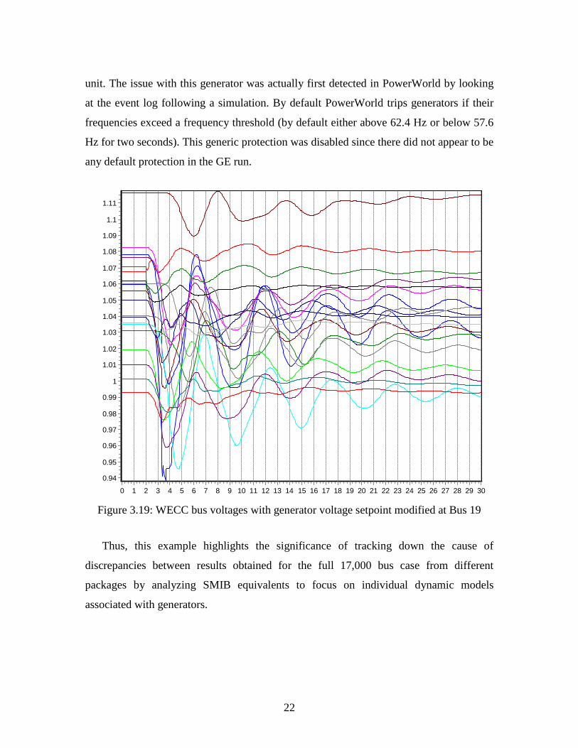
This was confirmed by re-running the WECC Case 4 with the Bus 19 voltage setpoint
increased from 1.0 to 1.02 per unit (which corresponds to a generator output of -4.4
Mvar), with the voltage results shown in Figure 3.19. Note that, in the WECC Case 2 that
was tested, the Bus 19 voltage setpoint was 1.03 per unit.
From the point of view of validation, we note that both PSLF and PowerWorld
appeared to correctly model the Bus 19 generator instability. One really cannot expect
accuracy for such an unusual operating condition in which the voltages are below 0.5 per
22
unit. The issue with this generator was actually first detected in PowerWorld by looking
at the event log following a simulation. By default PowerWorld trips generators if their
frequencies exceed a frequency threshold (by default either above 62.4 Hz or below 57.6
Hz for two seconds). This generic protection was disabled since there did not appear to be
any default protection in the GE run.
Figure 3.19: WECC bus voltages with generator voltage setpoint modified at Bus 19
Thus, this example highlights the significance of tracking down the cause of
discrepancies between results obtained for the full 17,000 bus case from different
packages by analyzing SMIB equivalents to focus on individual dynamic models
associated with generators.
3029282726252423222120191817161514131211109876543210
1.11
1.1
1.09
1.08
1.07
1.06
1.05
1.04
1.03
1.02
1.01
1
0.99
0.98
0.97
0.96
0.95
0.94
23
4. Validation Using Single Machine Infinite Bus Equivalents / Bottom-Up Approach
4.1 Background
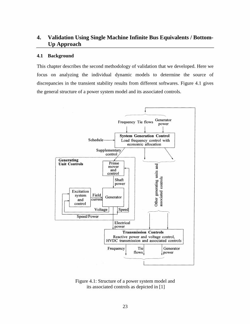
This chapter describes the second methodology of validation that we developed. Here we
focus on analyzing the individual dynamic models to determine the source of
discrepancies in the transient stability results from different softwares. Figure 4.1 gives
the general structure of a power system model and its associated controls.
Figure 4.1: Structure of a power system model and its associated controls as depicted in [1]

24
We focus on the generating unit subsystem. The various dynamic models associated
with a generating unit are listed below.
• Synchronous Machine Model: This is the most fundamental model used to
represent the dynamics associated with a generator. It models the equations of motion of
the generator, the rotor circuit dynamic equations and stator voltage equations.
• Excitation System: This system supplies direct current to the synchronous
machine field winding. Additionally, by controlling the field voltage, it controls the
voltage and reactive power flow. This system also performs critical protective functions
like ensuring that the capability limits of the synchronous machine and other equipment
are not violated. The basic elements of an excitation system include the Exciter, the
Voltage Regulator, Limiters and Protective Devices and the Power System Stabilizer. In
this chapter, we analyze some exciters in detail as well as a particular stabilizer model
used commonly in the WECC system.
• Prime Mover and Governor: The prime movers convert raw sources of energy
such as hydro and thermal energy into mechanical energy that is supplied to the
synchronous generators to produce electrical energy. The governor essentially controls
the power and frequency. In the subsequent chapters, we analyze certain governor models
existing in the WECC system.
Apart from these two types of models, a generator model may be associated with
other models like Turbine Load Controllers, Compensators, Over Excitation Limiters,
etc. Certain loads such as motors are also represented by particular dynamic models. The
focus of this work, though, is purely on the generation side.
The full WECC case has a total of 17,709 dynamic models in 77 model types. But the
20 most common model types contain 15,949 (90%) of these models. These are the key
focus areas for the bottom-up analysis, which is discussed in the following sections.
The approach can be briefly described as follows. First, we validated SMIB
equivalents consisting of only the machine model, to isolate it from any other potential
source of error. Then, to the validated machine models, we add elements such as an
25
exciter or a governor. Any discrepancies found in the SMIB results can then be attributed
to that particular model. Once the exciter has been validated, we can add a stabilizer to
correctly analyze it. Thus we can go on adding models to the machine model in an SMIB
equivalent one at a time and validate a new type of model at each step. This methodology
forms the crux of the bottom-up approach.
4.2 Machine Model Validation
In WECC Case 4, there are a total of 3308 machine models in the whole system. The
Round Rotor Generator Model with Quadratic Saturation (GENROU) and the Salient
Pole Generator Model with Quadratic Saturation on d-Axis (GENSAL) account for two-
thirds of these 3308 machine models. Hence validating these key models will certainly
have a big impact in providing validation of the generators in the WECC system.
4.2.1 GENROU – Round Rotor Generator Model with Quadratic Saturation
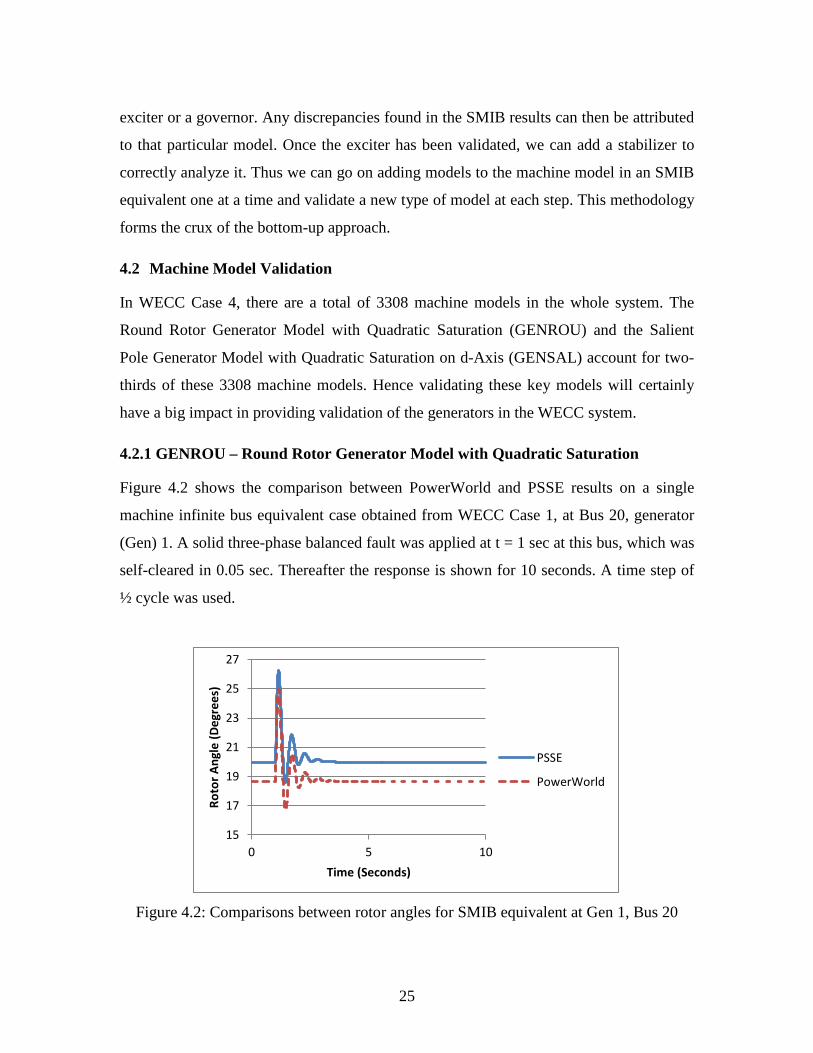
Figure 4.2 shows the comparison between PowerWorld and PSSE results on a single
machine infinite bus equivalent case obtained from WECC Case 1, at Bus 20, generator
(Gen) 1. A solid three-phase balanced fault was applied at t = 1 sec at this bus, which was
self-cleared in 0.05 sec. Thereafter the response is shown for 10 seconds. A time step of
½ cycle was used.
Figure 4.2: Comparisons between rotor angles for SMIB equivalent at Gen 1, Bus 20
15
17
19
21
23
25
27
0 5 10
Roto
r Ang
le (D
egre
es)
Time (Seconds)
PSSE
PowerWorld
26
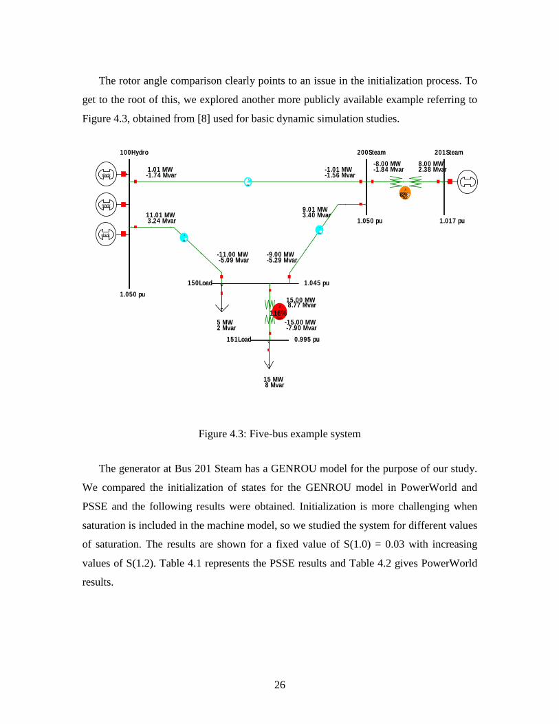
The rotor angle comparison clearly points to an issue in the initialization process. To
get to the root of this, we explored another more publicly available example referring to
Figure 4.3, obtained from [8] used for basic dynamic simulation studies.
Figure 4.3: Five-bus example system
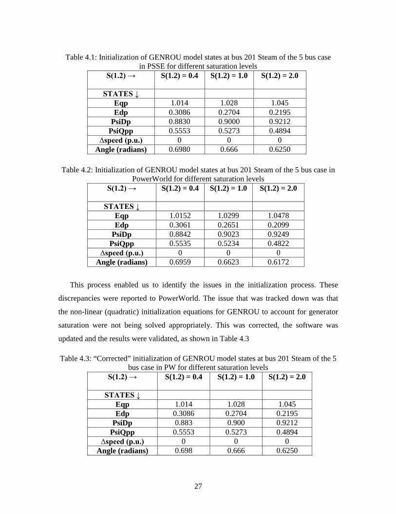
The generator at Bus 201 Steam has a GENROU model for the purpose of our study.
We compared the initialization of states for the GENROU model in PowerWorld and
PSSE and the following results were obtained. Initialization is more challenging when
saturation is included in the machine model, so we studied the system for different values
of saturation. The results are shown for a fixed value of S(1.0) = 0.03 with increasing
values of S(1.2). Table 4.1 represents the PSSE results and Table 4.2 gives PowerWorld
results.
slack
slack
slack
100Hydro 200Steam 201Steam
150Load
151Load
5 MW 2 Mvar
A
Amps
A
MVA
A
MVA
15 MW 8 Mvar
1.045 pu
1.050 pu 1.017 pu
1.050 pu
0.995 pu
1.01 MW -1.01 MW
11.01 MW
-11.00 MW
-8.00 MW 8.00 MW
-9.00 MW
9.01 MW
15.00 MW
-15.00 MW
-1.74 Mvar -1.56 Mvar
3.24 Mvar
-5.09 Mvar -5.29 Mvar
3.40 Mvar
8.77 Mvar
-7.90 Mvar
-1.84 Mvar 2.38 Mvar
82%A
MVA
116%A
MVA
27
Table 4.1: Initialization of GENROU model states at bus 201 Steam of the 5 bus case in PSSE for different saturation levels
S(1.2) →
S(1.2) = 0.4 S(1.2) = 1.0 S(1.2) = 2.0
STATES ↓ Eqp 1.014 1.028 1.045 Edp 0.3086 0.2704 0.2195
PsiDp 0.8830 0.9000 0.9212 PsiQpp 0.5553 0.5273 0.4894
∆speed (p.u.) 0 0 0 Angle (radians) 0.6980 0.666 0.6250
Table 4.2: Initialization of GENROU model states at bus 201 Steam of the 5 bus case in PowerWorld for different saturation levels
S(1.2) →
S(1.2) = 0.4 S(1.2) = 1.0 S(1.2) = 2.0
STATES ↓ Eqp 1.0152 1.0299 1.0478 Edp 0.3061 0.2651 0.2099
PsiDp 0.8842 0.9023 0.9249 PsiQpp 0.5535 0.5234 0.4822
∆speed (p.u.) 0 0 0 Angle (radians) 0.6959 0.6623 0.6172
This process enabled us to identify the issues in the initialization process. These
discrepancies were reported to PowerWorld. The issue that was tracked down was that
the non-linear (quadratic) initialization equations for GENROU to account for generator
saturation were not being solved appropriately. This was corrected, the software was
updated and the results were validated, as shown in Table 4.3
Table 4.3: “Corrected” initialization of GENROU model states at bus 201 Steam of the 5 bus case in PW for different saturation levels
S(1.2) →
S(1.2) = 0.4 S(1.2) = 1.0 S(1.2) = 2.0
STATES ↓ Eqp 1.014 1.028 1.045 Edp 0.3086 0.2704 0.2195
PsiDp 0.883 0.900 0.9212 PsiQpp 0.5553 0.5273 0.4894
∆speed (p.u.) 0 0 0 Angle (radians) 0.698 0.666 0.6250
28
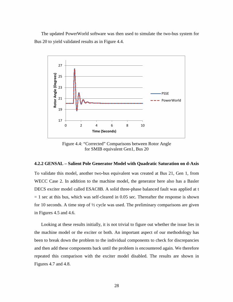
The updated PowerWorld software was then used to simulate the two-bus system for
Bus 20 to yield validated results as in Figure 4.4.
Figure 4.4: “Corrected” Comparisons between Rotor Angle
for SMIB equivalent Gen1, Bus 20
4.2.2 GENSAL – Salient Pole Generator Model with Quadratic Saturation on d-Axis
To validate this model, another two-bus equivalent was created at Bus 21, Gen 1, from
WECC Case 2. In addition to the machine model, the generator here also has a Basler
DECS exciter model called ESAC8B. A solid three-phase balanced fault was applied at t
= 1 sec at this bus, which was self-cleared in 0.05 sec. Thereafter the response is shown
for 10 seconds. A time step of ½ cycle was used. The preliminary comparisons are given
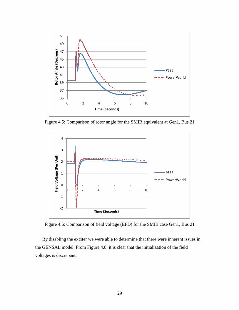
in Figures 4.5 and 4.6.
Looking at these results initially, it is not trivial to figure out whether the issue lies in
the machine model or the exciter or both. An important aspect of our methodology has
been to break down the problem to the individual components to check for discrepancies
and then add these components back until the problem is encountered again. We therefore
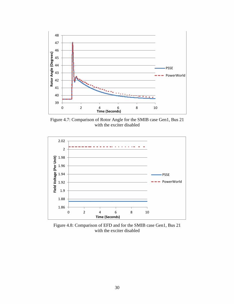
repeated this comparison with the exciter model disabled. The results are shown in
Figures 4.7 and 4.8.
17
19
21
23
25
27
0 2 4 6 8 10
Roto
r Ang
le (D
egre
es)
Time (Seconds)
PSSE
PowerWorld
29
Figure 4.5: Comparison of rotor angle for the SMIB equivalent at Gen1, Bus 21
Figure 4.6: Comparison of field voltage (EFD) for the SMIB case Gen1, Bus 21
By disabling the exciter we were able to determine that there were inherent issues in
the GENSAL model. From Figure 4.8, it is clear that the initialization of the field
voltages is discrepant.
35
37
39
41
43
45
47
49
51
0 2 4 6 8 10
Roto
r Ang
le (D
egre
es)
Time (Seconds)
PSSE
PowerWorld
-2
-1
0
1
2
3
4
0 2 4 6 8 10Fiel
d Vo
ltage
(Per
Uni
t)
Time (Seconds)
PSSE
PowerWorld
30
Figure 4.7: Comparison of Rotor Angle for the SMIB case Gen1, Bus 21
with the exciter disabled
Figure 4.8: Comparison of EFD and for the SMIB case Gen1, Bus 21
with the exciter disabled
39
40
41
42
43
44
45
46
47
48
0 2 4 6 8 10
Roto
r Ang
le (D
egre
es)
Time (Seconds)
PSSE
PowerWorld
1.86
1.88
1.9
1.92
1.94
1.96
1.98
2
2.02
0 2 4 6 8 10
Fiel
d Vo
ltage
(Per
Uni
t)
Time (Seconds)
PSSE
PowerWorld
31
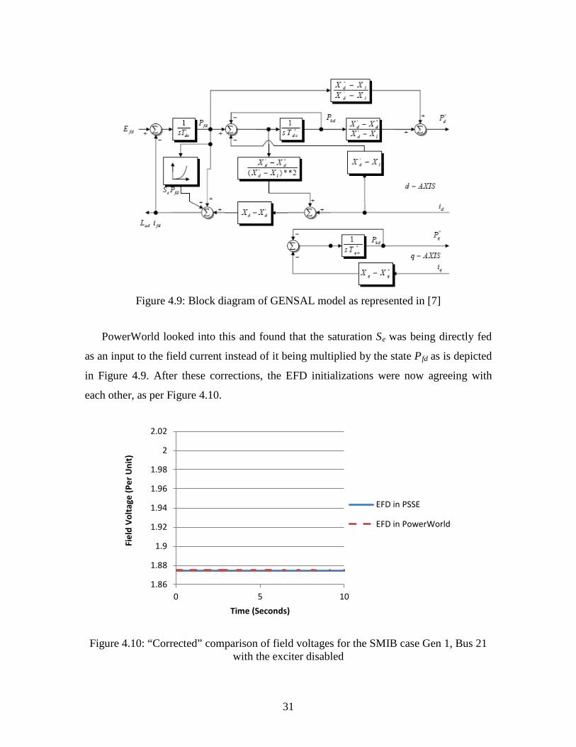
Figure 4.9: Block diagram of GENSAL model as represented in [7]
PowerWorld looked into this and found that the saturation Se was being directly fed
as an input to the field current instead of it being multiplied by the state Pfd as is depicted
in Figure 4.9. After these corrections, the EFD initializations were now agreeing with
each other, as per Figure 4.10.
Figure 4.10: “Corrected” comparison of field voltages for the SMIB case Gen 1, Bus 21
with the exciter disabled
1.86
1.88
1.9
1.92
1.94
1.96
1.98
2
2.02
0 5 10
Fiel
d Vo
ltage
(Per
Uni
t)
Time (Seconds)
EFD in PSSE
EFD in PowerWorld
32
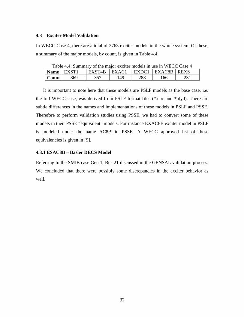
4.3 Exciter Model Validation
In WECC Case 4, there are a total of 2763 exciter models in the whole system. Of these,
a summary of the major models, by count, is given in Table 4.4.
Table 4.4: Summary of the major exciter models in use in WECC Case 4 Name EXST1 EXST4B EXAC1 EXDC1 EXAC8B REXS Count 869 357 149 288 166 231
It is important to note here that these models are PSLF models as the base case, i.e.
the full WECC case, was derived from PSLF format files (*.epc and *.dyd). There are
subtle differences in the names and implementations of these models in PSLF and PSSE.
Therefore to perform validation studies using PSSE, we had to convert some of these
models in their PSSE “equivalent” models. For instance EXAC8B exciter model in PSLF
is modeled under the name AC8B in PSSE. A WECC approved list of these
equivalencies is given in [9].
4.3.1 ESAC8B – Basler DECS Model
Referring to the SMIB case Gen 1, Bus 21 discussed in the GENSAL validation process.
We concluded that there were possibly some discrepancies in the exciter behavior as
well.
33
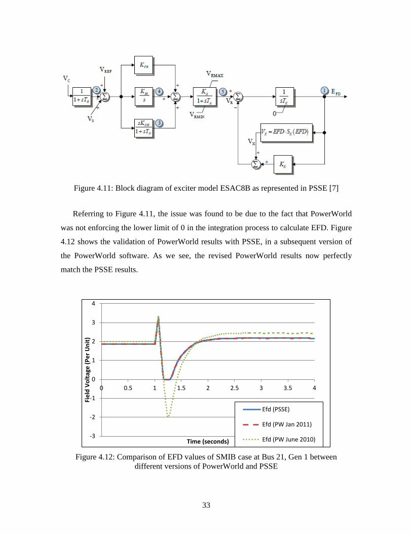
Figure 4.11: Block diagram of exciter model ESAC8B as represented in PSSE [7]
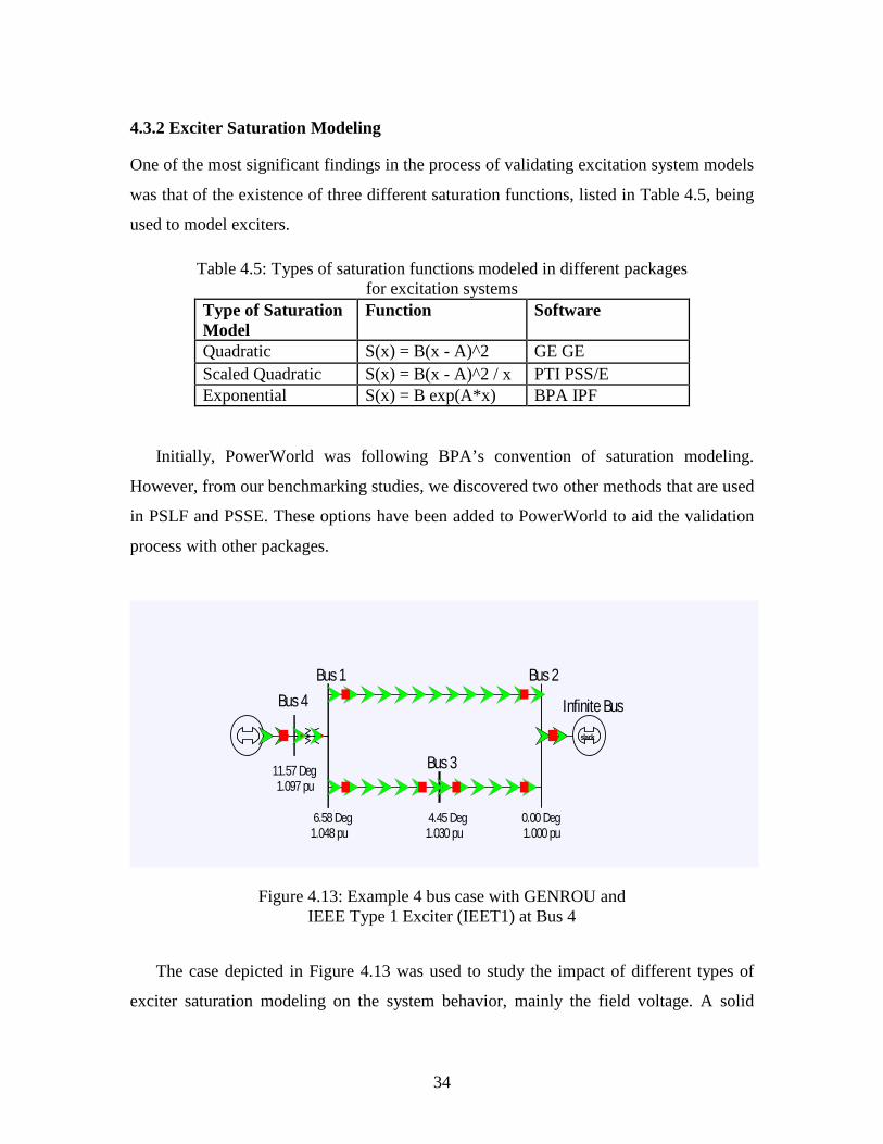
Referring to Figure 4.11, the issue was found to be due to the fact that PowerWorld
was not enforcing the lower limit of 0 in the integration process to calculate EFD. Figure
4.12 shows the validation of PowerWorld results with PSSE, in a subsequent version of
the PowerWorld software. As we see, the revised PowerWorld results now perfectly
match the PSSE results.
Figure 4.12: Comparison of EFD values of SMIB case at Bus 21, Gen 1 between
different versions of PowerWorld and PSSE
-3
-2
-1
0
1
2
3
4
0 0.5 1 1.5 2 2.5 3 3.5 4
Fiel
d Vo
ltage
(Per
Uni
t)
Time (seconds)
Efd (PSSE)
Efd (PW Jan 2011)
Efd (PW June 2010)
34
4.3.2 Exciter Saturation Modeling
One of the most significant findings in the process of validating excitation system models
was that of the existence of three different saturation functions, listed in Table 4.5, being
used to model exciters.
Table 4.5: Types of saturation functions modeled in different packages for excitation systems
Type of Saturation Model
Function Software
Quadratic S(x) = B(x - A)^2 GE GE Scaled Quadratic S(x) = B(x - A)^2 / x PTI PSS/E Exponential S(x) = B exp(A*x) BPA IPF
Initially, PowerWorld was following BPA’s convention of saturation modeling.
However, from our benchmarking studies, we discovered two other methods that are used
in PSLF and PSSE. These options have been added to PowerWorld to aid the validation
process with other packages.
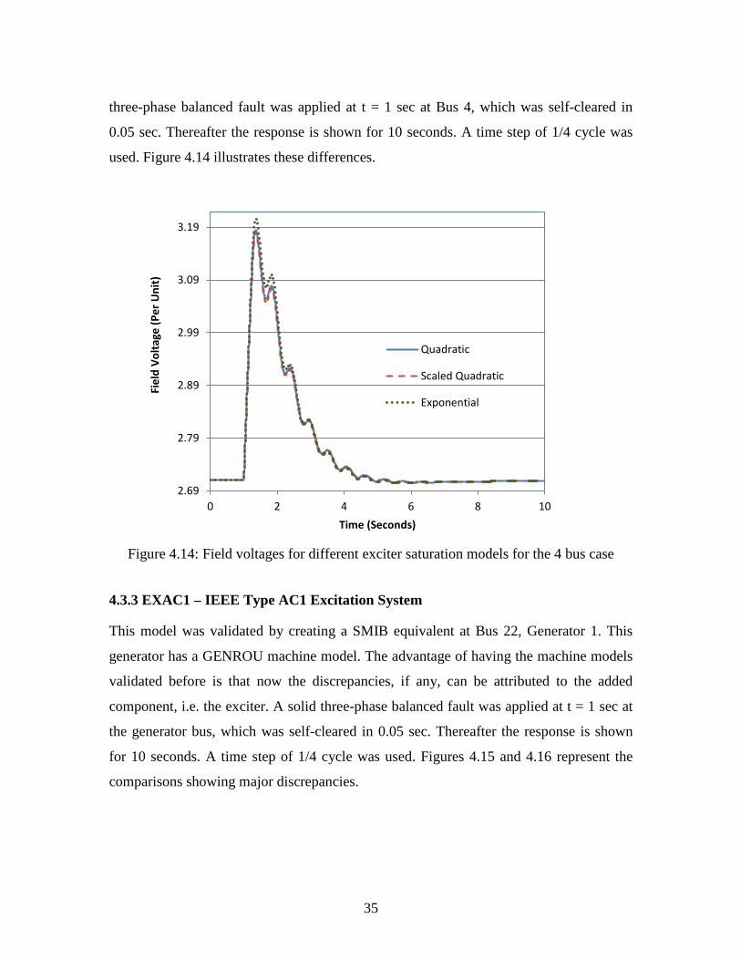
Figure 4.13: Example 4 bus case with GENROU and IEEE Type 1 Exciter (IEET1) at Bus 4
The case depicted in Figure 4.13 was used to study the impact of different types of
exciter saturation modeling on the system behavior, mainly the field voltage. A solid
Infinite Bus
slack
Bus 1 Bus 2
Bus 3
0.00 Deg 6.58 Deg
Bus 4
11.57 Deg
4.45 Deg 1.000 pu 1.030 pu 1.048 pu
1.097 pu
35
three-phase balanced fault was applied at t = 1 sec at Bus 4, which was self-cleared in
0.05 sec. Thereafter the response is shown for 10 seconds. A time step of 1/4 cycle was
used. Figure 4.14 illustrates these differences.
Figure 4.14: Field voltages for different exciter saturation models for the 4 bus case
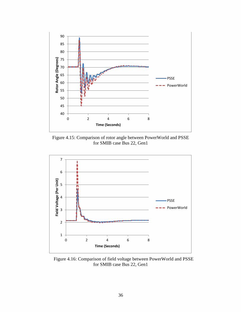
4.3.3 EXAC1 – IEEE Type AC1 Excitation System
This model was validated by creating a SMIB equivalent at Bus 22, Generator 1. This
generator has a GENROU machine model. The advantage of having the machine models
validated before is that now the discrepancies, if any, can be attributed to the added
component, i.e. the exciter. A solid three-phase balanced fault was applied at t = 1 sec at
the generator bus, which was self-cleared in 0.05 sec. Thereafter the response is shown
for 10 seconds. A time step of 1/4 cycle was used. Figures 4.15 and 4.16 represent the
comparisons showing major discrepancies.
2.69
2.79
2.89
2.99
3.09
3.19
0 2 4 6 8 10
Fiel
d Vo
ltage
(Per
Uni
t)
Time (Seconds)
Quadratic
Scaled Quadratic
Exponential
36
Figure 4.15: Comparison of rotor angle between PowerWorld and PSSE
for SMIB case Bus 22, Gen1
4.1Figure 4.16: Comparison of field voltage between PowerWorld and PSSE
for SMIB case Bus 22, Gen1
40
45
50
55
60
65
70
75
80
85
90
0 2 4 6 8
Roto
r Ang
le (D
egre
es)
Time (Seconds)
PSSE
PowerWorld
1
2
3
4
5
6
7
0 2 4 6 8
Fiel
d Vo
ltage
(Per
Uni
t)
Time (Seconds)
PSSE
PowerWorld
37
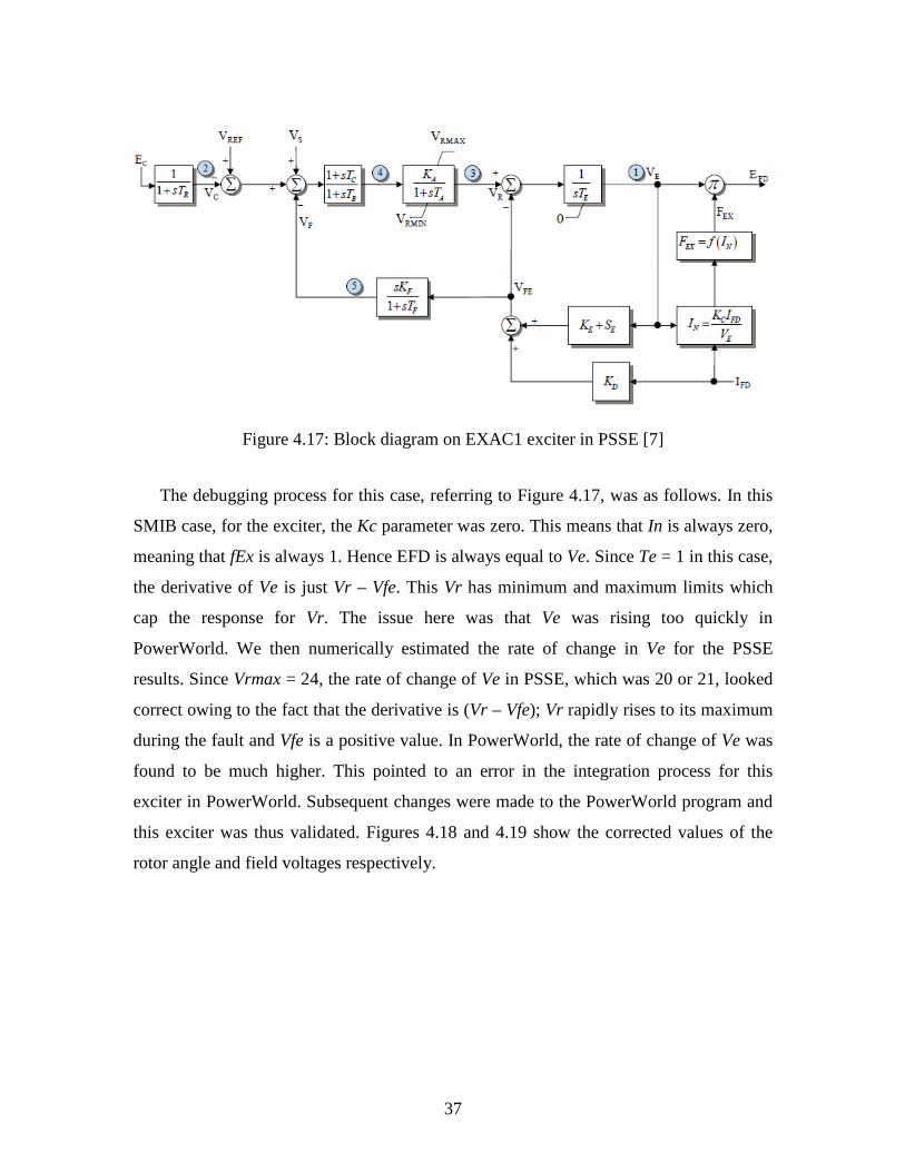
Figure 4.17: Block diagram on EXAC1 exciter in PSSE [7]
The debugging process for this case, referring to Figure 4.17, was as follows. In this
SMIB case, for the exciter, the Kc parameter was zero. This means that In is always zero,
meaning that fEx is always 1. Hence EFD is always equal to Ve. Since Te = 1 in this case,
the derivative of Ve is just Vr – Vfe. This Vr has minimum and maximum limits which
cap the response for Vr. The issue here was that Ve was rising too quickly in
PowerWorld. We then numerically estimated the rate of change in Ve for the PSSE
results. Since Vrmax = 24, the rate of change of Ve in PSSE, which was 20 or 21, looked
correct owing to the fact that the derivative is (Vr – Vfe); Vr rapidly rises to its maximum
during the fault and Vfe is a positive value. In PowerWorld, the rate of change of Ve was
found to be much higher. This pointed to an error in the integration process for this
exciter in PowerWorld. Subsequent changes were made to the PowerWorld program and
this exciter was thus validated. Figures 4.18 and 4.19 show the corrected values of the
rotor angle and field voltages respectively.
38
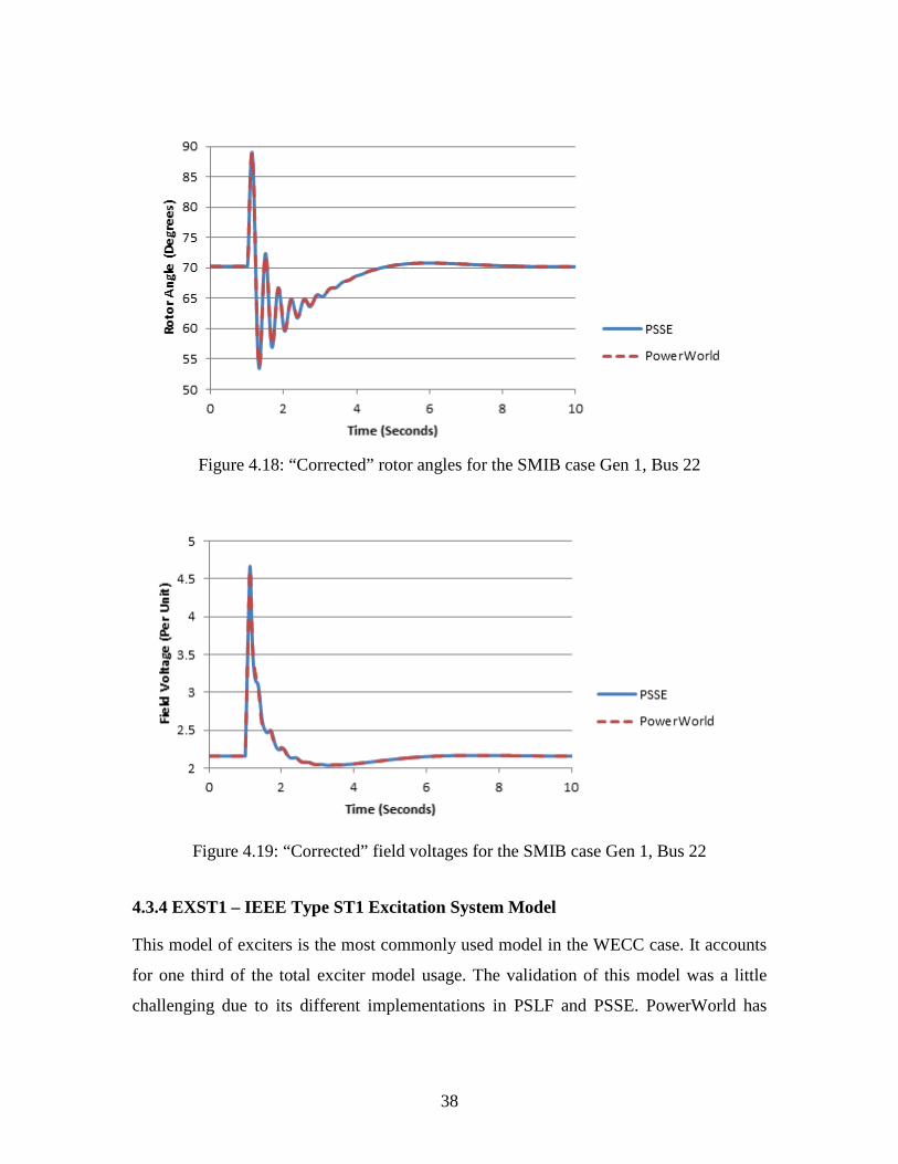
Figure 4.18: “Corrected” rotor angles for the SMIB case Gen 1, Bus 22
Figure 4.19: “Corrected” field voltages for the SMIB case Gen 1, Bus 22
4.3.4 EXST1 – IEEE Type ST1 Excitation System Model
This model of exciters is the most commonly used model in the WECC case. It accounts
for one third of the total exciter model usage. The validation of this model was a little
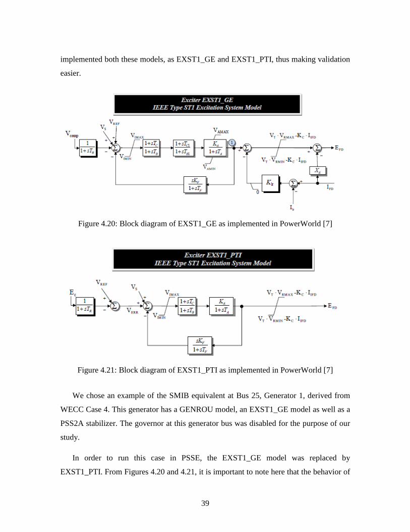
challenging due to its different implementations in PSLF and PSSE. PowerWorld has
39
implemented both these models, as EXST1_GE and EXST1_PTI, thus making validation
easier.
Figure 4.20: Block diagram of EXST1_GE as implemented in PowerWorld [7]
Figure 4.21: Block diagram of EXST1_PTI as implemented in PowerWorld [7]
We chose an example of the SMIB equivalent at Bus 25, Generator 1, derived from
WECC Case 4. This generator has a GENROU model, an EXST1_GE model as well as a
PSS2A stabilizer. The governor at this generator bus was disabled for the purpose of our
study.
In order to run this case in PSSE, the EXST1_GE model was replaced by
EXST1_PTI. From Figures 4.20 and 4.21, it is important to note here that the behavior of
40
these two exciter models will differ, unless there are no limits enforced on Va and unless
Tc1 = Tb1 = Klr = Xe = 0.
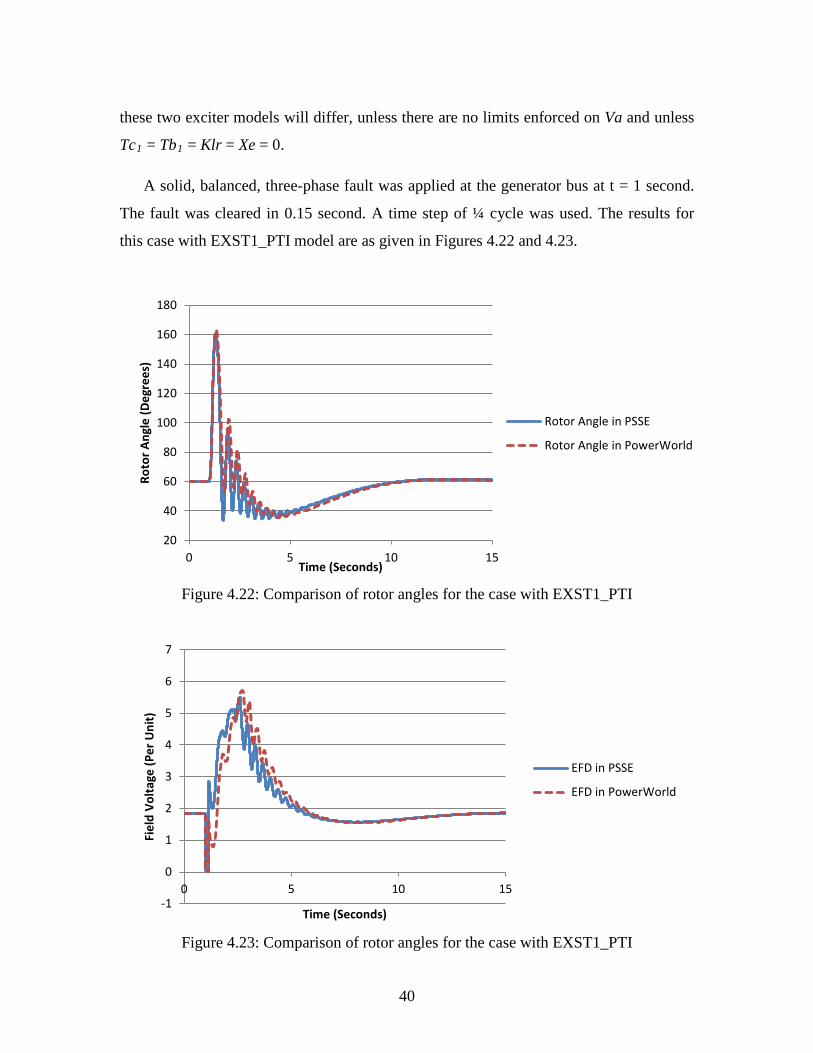
A solid, balanced, three-phase fault was applied at the generator bus at t = 1 second.
The fault was cleared in 0.15 second. A time step of ¼ cycle was used. The results for
this case with EXST1_PTI model are as given in Figures 4.22 and 4.23.
Figure 4.22: Comparison of rotor angles for the case with EXST1_PTI
Figure 4.23: Comparison of rotor angles for the case with EXST1_PTI
20
40
60
80
100
120
140
160
180
0 5 10 15
Roto
r Ang
le (D
egre
es)
Time (Seconds)
Rotor Angle in PSSE
Rotor Angle in PowerWorld
-1
0
1
2
3
4
5
6
7
0 5 10 15
Fiel
d Vo
ltage
(Per
Uni
t)
Time (Seconds)
EFD in PSSE
EFD in PowerWorld
41
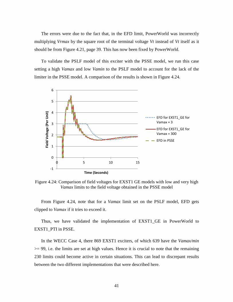
The errors were due to the fact that, in the EFD limit, PowerWorld was incorrectly
multiplying Vrmax by the square root of the terminal voltage Vt instead of Vt itself as it
should be from Figure 4.21, page 39. This has now been fixed by PowerWorld.
To validate the PSLF model of this exciter with the PSSE model, we run this case
setting a high Vamax and low Vamin to the PSLF model to account for the lack of the
limiter in the PSSE model. A comparison of the results is shown in Figure 4.24.
Figure 4.24: Comparison of field voltages for EXST1 GE models with low and very high
Vamax limits to the field voltage obtained in the PSSE model
From Figure 4.24, note that for a Vamax limit set on the PSLF model, EFD gets
clipped to Vamax if it tries to exceed it.
Thus, we have validated the implementation of EXST1_GE in PowerWorld to
EXST1_PTI in PSSE.
In the WECC Case 4, there 869 EXST1 exciters, of which 639 have the Vamax/min
>= 99, i.e. the limits are set at high values. Hence it is crucial to note that the remaining
230 limits could become active in certain situations. This can lead to discrepant results
between the two different implementations that were described here.
-1
0
1
2
3
4
5
6
0 5 10 15
Fiel
d Vo
ltage
(Per
Uni
t)
Time (Seconds)
EFD for EXST1_GE forVamax = 3
EFD for EXST1_GE forVamax = 300
EFD in PSSE
42
4.4 Stabilizer Model Validation
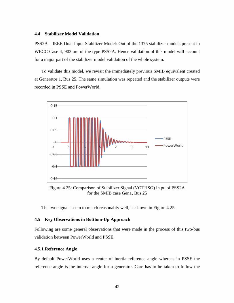
PSS2A – IEEE Dual Input Stabilizer Model: Out of the 1375 stabilizer models present in
WECC Case 4, 903 are of the type PSS2A. Hence validation of this model will account
for a major part of the stabilizer model validation of the whole system.
To validate this model, we revisit the immediately previous SMIB equivalent created
at Generator 1, Bus 25. The same simulation was repeated and the stabilizer outputs were
recorded in PSSE and PowerWorld.
Figure 4.25: Comparison of Stabilizer Signal (VOTHSG) in pu of PSS2A
for the SMIB case Gen1, Bus 25
The two signals seem to match reasonably well, as shown in Figure 4.25.
4.5 Key Observations in Botttom-Up Approach
Following are some general observations that were made in the process of this two-bus
validation between PowerWorld and PSSE.
4.5.1 Reference Angle
By default PowerWorld uses a center of inertia reference angle whereas in PSSE the
reference angle is the internal angle for a generator. Care has to be taken to follow the
43
same convention of reference angle to achieve proper validation of results of the same
system in two different software packages. PowerWorld provides several options to
choose angle reference in order to maintain compatibility with other software packages.
4.5.2 Generator Compensation
In PSLF and PowerWorld, generator compensation (Rcomp and Xcomp) values are
modeled as the parameters of the machine model. In PSSE, however, a separate
compensation model has to be associated with the machine model where these values can
be entered. This was one of the causes of a lot of discrepant results when *.raw and *.dyr
files were exported from PowerWorld to PSSE to perform validation. Before making any
such comparisons, either Rcomp and Xcomp should be set to 0 in the machine model in
PowerWorld or the compensator model with appropriate values should be added to the
machine model in PSSE.
44
5. Validation of Generator Saturation and Exciter Speed Dependence Using BPA Data
5.1 Validation of Generator Model Saturation Using BPA Data
In the previous chapter, GENROU and GENSAL models were validated between PSSE
and PowerWorld using two-bus equivalent systems. Based on the previous analysis these
models match quite closely. In this section, the PowerWorld GENROU, GENSAL and
GENTPF models were validated with the PSLF models using the generator field current
values for a number of BPA generators (at initialization the field current is identical to
the field voltage).
Since the initial field current is sensitive to the generator’s reactive power output, the
first step in the comparison was to determine how closely these values matched. Using
the stored generator reactive power outputs for the *.epc input file and the solved
PowerWorld case, the match was quite good, but not always exact. For the 2580 online
generators in the case, only six had differences above 10 Mvar, 117 above 1 Mvar and a
total of 132 above 0.5 Mvar. While the reason for these power flow differences is beyond
the scope of the study, it is mostly likely due to differences in how reactive power is
shared between generators regulating the same bus.
Without correcting for the power flow reactive power injection differences, there can
be substantial differences in the field current that have nothing to do with the transient
stability models. For example at the bus 39 generator there is a 9.8 Mvar difference,
resulting in a 0.04 per unit field current difference. These differences become more
significant for the lower MVA units. To remove this bias, the generator power flow
reactive outputs in the PowerWorld case were modified to exactly match the PSLF case
values for the 78 BPA units in which the value was above 0.5 Mvars.
In performing the generator field voltage validation, it was noted that sometimes the
PSSE and PSLF models gave slightly different results. While the differences were not
large (usually less than one percent), they were large enough to require investigation. The
result is that the differences appear to be due to a difference between the PSLF and PSSE
implementations of generator saturation modeling for the GENSAL and GENROU
45
models (PSSE currently does not have an equivalent for the GENTPF and GENTPJ
models). Both models use a quadratic model in which the amount of saturation is inputted
at values of 1.0 and 1.2 (with these saturation values denoted as S1 and S12). For the
GENSAL model the saturation is a function of the Eqp (the direct-axis transient flux),
whereas for the GENROU model it is a function of the total sub-transient flux.
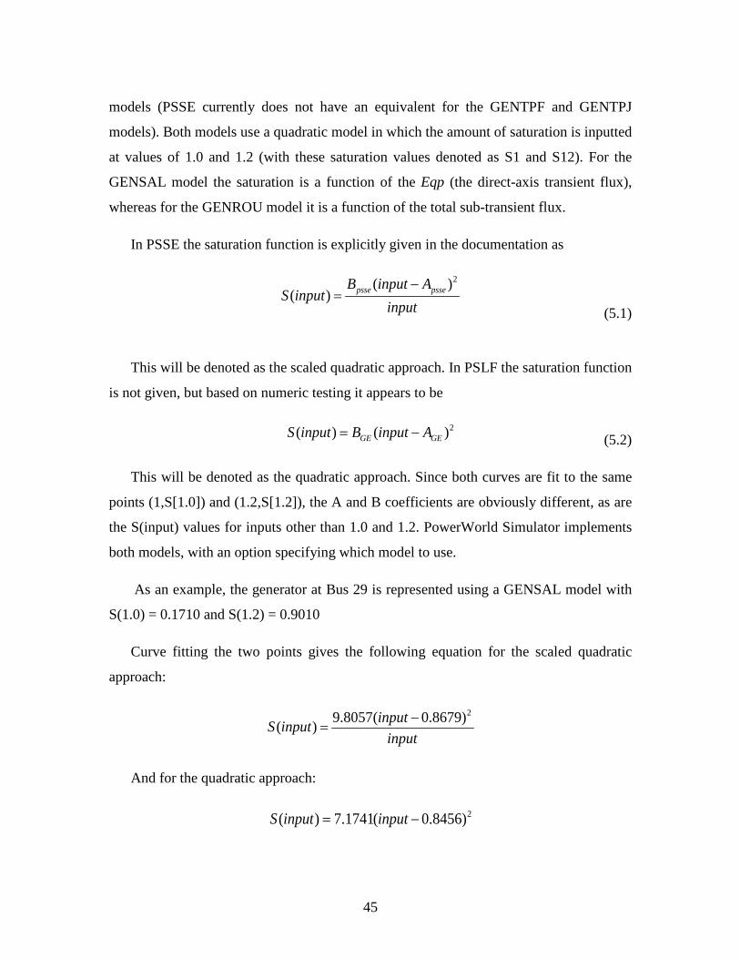
In PSSE the saturation function is explicitly given in the documentation as
2( )( ) psse psseB input A
S inputinput
−=
(5.1)
This will be denoted as the scaled quadratic approach. In PSLF the saturation function
is not given, but based on numeric testing it appears to be
2( ) ( )GE GES input B input A= − (5.2)
This will be denoted as the quadratic approach. Since both curves are fit to the same
points (1,S[1.0]) and (1.2,S[1.2]), the A and B coefficients are obviously different, as are
the S(input) values for inputs other than 1.0 and 1.2. PowerWorld Simulator implements
both models, with an option specifying which model to use.
As an example, the generator at Bus 29 is represented using a GENSAL model with
S(1.0) = 0.1710 and S(1.2) = 0.9010
Curve fitting the two points gives the following equation for the scaled quadratic
approach:
29.8057( 0.8679)( ) inputS inputinput
−=
And for the quadratic approach:
2( ) 7.1741( 0.8456)S input input= −
46
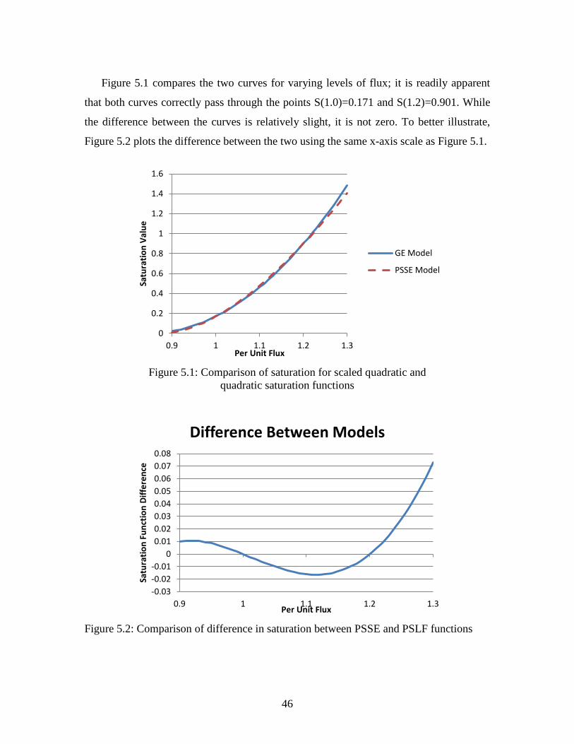
Figure 5.1 compares the two curves for varying levels of flux; it is readily apparent
that both curves correctly pass through the points S(1.0)=0.171 and S(1.2)=0.901. While
the difference between the curves is relatively slight, it is not zero. To better illustrate,
Figure 5.2 plots the difference between the two using the same x-axis scale as Figure 5.1.
Figure 5.1: Comparison of saturation for scaled quadratic and
quadratic saturation functions
Figure 5.2: Comparison of difference in saturation between PSSE and PSLF functions
0
0.2
0.4
0.6
0.8
1
1.2
1.4
1.6
0.9 1 1.1 1.2 1.3
Satu
ratio
n Va
lue
Per Unit Flux
GE Model
PSSE Model
-0.03-0.02-0.01
00.010.020.030.040.050.060.070.08
0.9 1 1.1 1.2 1.3
Satu
ratio
n Fu
nctio
n Di
ffere
nce
Per Unit Flux
Difference Between Models

47
The difference in the saturation values for fluxes other than 1.0 and 1.2 results in
differences in the field voltage and subsequently in the exciter state variable values. For
the bus 29 example, in which the initial per unit flux is 1.051, the scaled quadratic gives
an initial field voltage of 2.5137 (based on results using a two bus equivalent) while the
quadratic gives a value of 2.5034 (based on results from the WECC Case 4). Note that
that -0.0103 difference is quite close to what would be expected from Figure 5.2. The
initial field voltage is 2.5147 in PowerWorld when solved with the scaled quadratic
saturation modeling and 2.5036 when solved with the quadratic approach, with both
values closely matching those from the other two programs.
A second example is for the two generators at bus 30 in which the generator 1 and 2
initial field voltages are 1.6445 and 1.5561 in PSSE and 1.6394 and 1.5506 in PSLF.
Solving in PowerWorld, the values are 1.6430 and 1.5543 using the scaled quadratic
(PSSE) approach, and 1.6401 and 1.5513 using the quadratic (PSLF) approach; again all
closely match.
To validate this approach, the initial field current values for the 200 largest on-line
generators (in terms of real power output) in BPA (for which we had data) were
compared. Using the quadratic saturation function the average error in the initial field
current values was 0.0084 per unit, while with the scaled quadratic saturation function the
average error was 0.01223 per unit. If the values are limited to just the 100 largest units,
for which small initial differences in the power flow reactive power output would have
the least affect, the average was 0.0031 per unit for the quadratic approach and 0.0083 for
the scaled quadratic. Since the actual PSLF values were only available with a precision of
0.001, the conclusion appears to be that (1) the PowerWorld software closely matches the
initial field values from PSLF, and (2) the quadratic approach is the best way to match
the PSLF results.
Since PowerWorld implements both approaches, the significance of the issue can be
studied. In the WECC model there are 2533 generators with active generator models. The
largest difference in the initial field voltage between the two models is 0.0339 per unit (at
the generator at bus 31), with only five generators having differences above 0.03, a total
48
of 23 having differences above 0.02 and a total of 111 above 0.01 per unit. In terms of
percentage, the largest difference is 1.66% at 31, with 25 generators having differences
above 1.0%.
This issue is not considered significant, but it does need to be considered during
validation between the different packages since differences in the field voltages can get
amplified into differences in the initial exciter values.
5.2 Validation of Exciters Using BPA Data
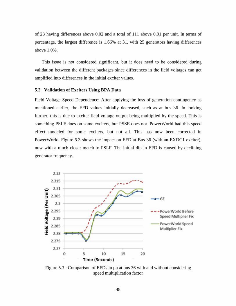
Field Voltage Speed Dependence: After applying the loss of generation contingency as
mentioned earlier, the EFD values initially decreased, such as at bus 36. In looking
further, this is due to exciter field voltage output being multiplied by the speed. This is
something PSLF does on some exciters, but PSSE does not. PowerWorld had this speed
effect modeled for some exciters, but not all. This has now been corrected in
PowerWorld. Figure 5.3 shows the impact on EFD at Bus 36 (with an EXDC1 exciter),
now with a much closer match to PSLF. The initial dip in EFD is caused by declining
generator frequency.
Figure 5.3 : Comparison of EFDs in pu at bus 36 with and without considering
speed multiplication factor
49
6. Time Step Comparisons
Throughout the course of this work, we have mostly used a time step of ¼ cycle since it
is the WECC standard. However, in light of the discussion in Chapter 3, it would be
interesting to study the system response using different time steps and the corresponding
time constant auto-corrections.
In the time step comparison study, we used WECC Case 4. The loss of the same units
as simulated earlier was the contingency applied at t = 2 seconds. We used time steps of
¼ cycle and ½ cycle for our comparisons. The simulation was run for a total of 30
seconds.
On “running validation” on this case for each of these time steps, the validation
statistics given in Table 6.1 were obtained in PowerWorld.
Table 6.1: Summary of validation messages obtained for WECC Case 4, using different time steps
Time Step
↓
Validation message fields
→
Validation Errors
Validation Warnings
Validation Warnings after
Auto-Correction ¼ cycle 941 41 39 ½ cycle 3038 43 41
The large number of validation errors in the instance where ½ cycle is used is
intuitive as the most of the time constants of the WECC case must be designed for the
standard time step of ¼ cycle. A majority of the auto-corrections consist of those for the
time constants, the remaining being reactance and saturation values as discussed in
Chapter 2.
The solution statistics using these two different time steps are given in Table 6.2. The
network solution statistics are represented by the number of forward/backwards
substitutions and Jacobian factorizations.
50
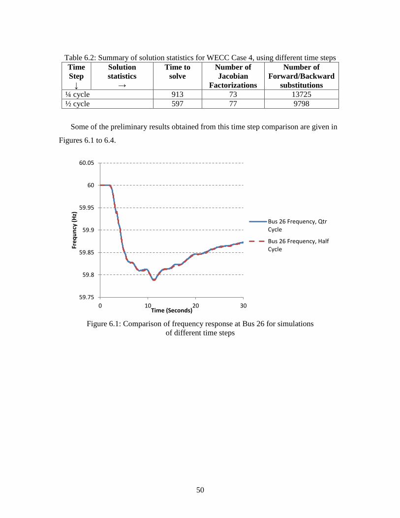
Table 6.2: Summary of solution statistics for WECC Case 4, using different time steps Time Step
↓
Solution statistics
→
Time to solve
Number of Jacobian
Factorizations
Number of Forward/Backward
substitutions ¼ cycle 913 73 13725 ½ cycle 597 77 9798
Some of the preliminary results obtained from this time step comparison are given in
Figures 6.1 to 6.4.
Figure 6.1: Comparison of frequency response at Bus 26 for simulations
of different time steps
59.75
59.8
59.85
59.9
59.95
60
60.05
0 10 20 30
Freq
uncy
(Hz)
Time (Seconds)
Bus 26 Frequency, QtrCycle
Bus 26 Frequency, HalfCycle
51
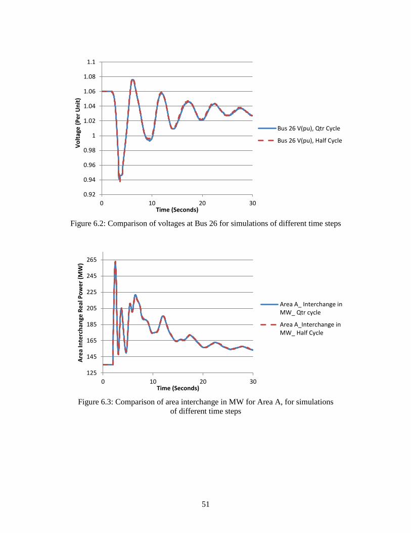
Figure 6.2: Comparison of voltages at Bus 26 for simulations of different time steps
Figure 6.3: Comparison of area interchange in MW for Area A, for simulations
of different time steps
0.92
0.94
0.96
0.98
1
1.02
1.04
1.06
1.08
1.1
0 10 20 30
Volta
ge (P
er U
nit)
Time (Seconds)
Bus 26 V(pu), Qtr Cycle
Bus 26 V(pu), Half Cycle
125
145
165
185
205
225
245
265
0 10 20 30
Area
Inte
rcha
nge
Real
Pow
er (M
W)
Time (Seconds)
Area A_ Interchange inMW_ Qtr cycle
Area A_Interchange inMW_ Half Cycle
52
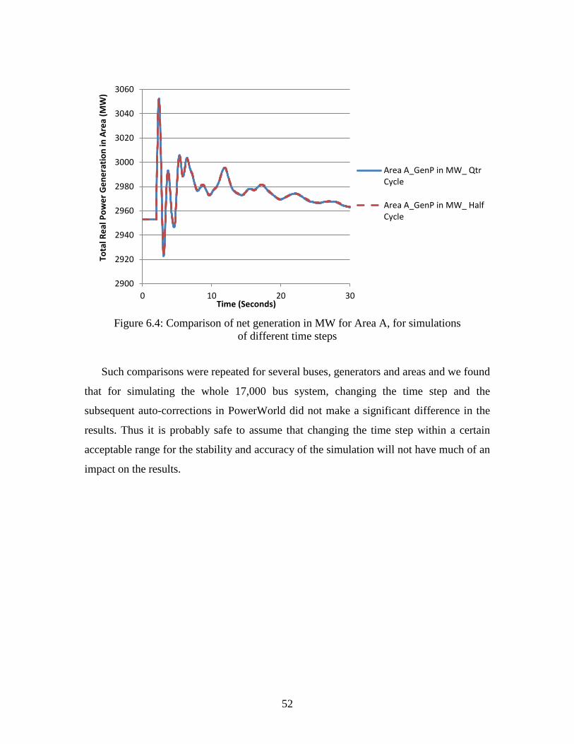
Figure 6.4: Comparison of net generation in MW for Area A, for simulations
of different time steps
Such comparisons were repeated for several buses, generators and areas and we found
that for simulating the whole 17,000 bus system, changing the time step and the
subsequent auto-corrections in PowerWorld did not make a significant difference in the
results. Thus it is probably safe to assume that changing the time step within a certain
acceptable range for the stability and accuracy of the simulation will not have much of an
impact on the results.
2900
2920
2940
2960
2980
3000
3020
3040
3060
0 10 20 30
Tota
l Rea
l Pow
er G
ener
atio
n in
Are
a (M
W)
Time (Seconds)
Area A_GenP in MW_ QtrCycle
Area A_GenP in MW_ HalfCycle
53
7. Frequency Comparisons of WECC Case 4
7.1 Overview
This chapter covers the comparison of results between PowerWorld (version 16 beta) and
PSLF (version 17) for WECC Case 4, consisting of 17710 buses and 3470 generators.
The tested scenario is the loss of the same generating units, as studied earlier. For the
simulations, the system was initially allowed to run unperturbed for two seconds to
demonstrate a stable initial contingency. Then the contingency was applied at time t = 2.0
seconds and the simulation run for a total of 30 seconds. Both cases were integrated using
a ¼ cycle time step.
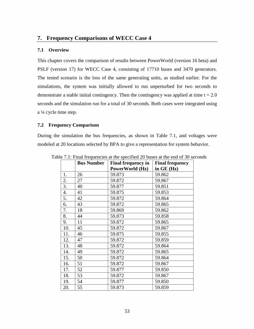
7.2 Frequency Comparison
During the simulation the bus frequencies, as shown in Table 7.1, and voltages were
modeled at 20 locations selected by BPA to give a representation for system behavior.
1 Table 7.1: Final frequencies at the specified 20 buses at the end of 30 seconds Bus Number Final frequency in
PowerWorld (Hz) Final frequency in GE (Hz)
1. 26 59.873 59.862 2. 27 59.872 59.867 3. 40 59.877 59.851 4. 41 59.875 59.853 5. 42 59.872 59.864 6. 43 59.872 59.865 7. 18 59.869 59.862 8. 44 59.873 59.858 9. 11 59.872 59.865 10. 45 59.872 59.867 11. 46 59.875 59.855 12. 47 59.872 59.859 13. 48 59.872 59.864 14. 49 59.872 59.865 15. 50 59.872 59.864 16. 51 59.872 59.867 17. 52 59.877 59.850 18. 53 59.872 59.867 19. 54 59.877 59.850 20. 55 59.873 59.859
54
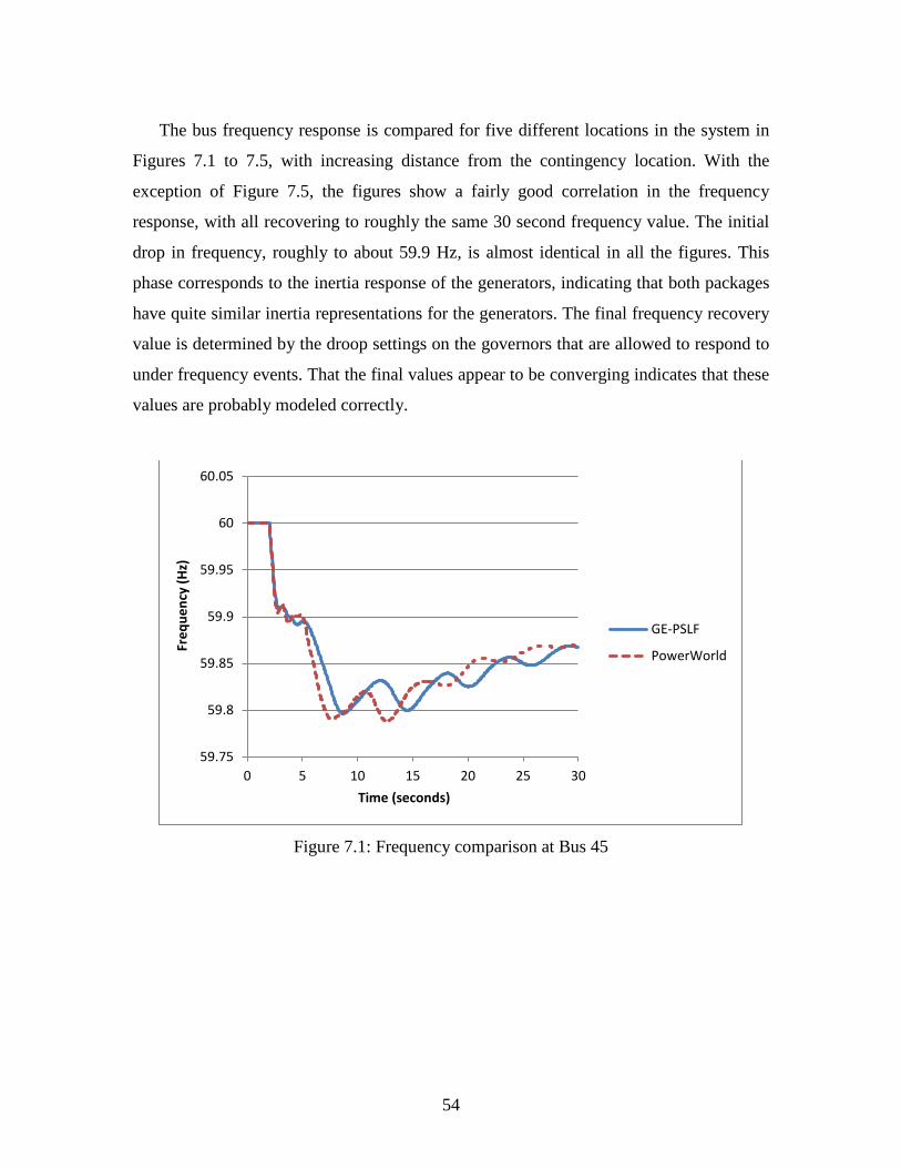
The bus frequency response is compared for five different locations in the system in
Figures 7.1 to 7.5, with increasing distance from the contingency location. With the
exception of Figure 7.5, the figures show a fairly good correlation in the frequency
response, with all recovering to roughly the same 30 second frequency value. The initial
drop in frequency, roughly to about 59.9 Hz, is almost identical in all the figures. This
phase corresponds to the inertia response of the generators, indicating that both packages
have quite similar inertia representations for the generators. The final frequency recovery
value is determined by the droop settings on the governors that are allowed to respond to
under frequency events. That the final values appear to be converging indicates that these
values are probably modeled correctly.
Figure 7.1: Frequency comparison at Bus 45
59.75
59.8
59.85
59.9
59.95
60
60.05
0 5 10 15 20 25 30
Freq
uenc
y (H
z)
Time (seconds)
GE-PSLF
PowerWorld
55
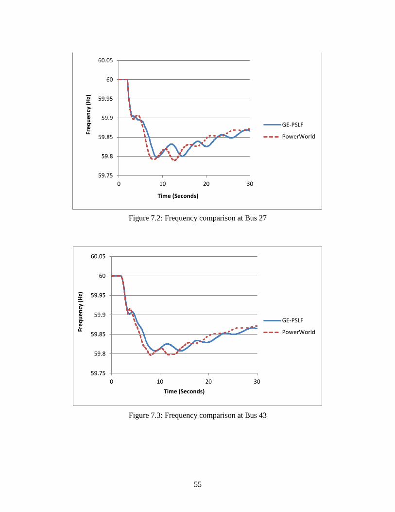
Figure 7.2: Frequency comparison at Bus 27
Figure 7.3: Frequency comparison at Bus 43
59.75
59.8
59.85
59.9
59.95
60
60.05
0 10 20 30
Freq
uenc
y (H
z)
Time (Seconds)
GE-PSLF
PowerWorld
59.75
59.8
59.85
59.9
59.95
60
60.05
0 10 20 30
Freq
uenc
y (H
z)
Time (Seconds)
GE-PSLF
PowerWorld
56
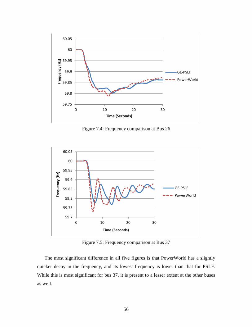
Figure 7.4: Frequency comparison at Bus 26
Figure 7.5: Frequency comparison at Bus 37
The most significant difference in all five figures is that PowerWorld has a slightly
quicker decay in the frequency, and its lowest frequency is lower than that for PSLF.
While this is most significant for bus 37, it is present to a lesser extent at the other buses
as well.
59.75
59.8
59.85
59.9
59.95
60
60.05
0 10 20 30
Freq
uenc
y (H
z)
Time (Seconds)
GE-PSLF
PowerWorld
59.7
59.75
59.8
59.85
59.9
59.95
60
60.05
0 10 20 30
Freq
uenc
y (H
z)
Time (Seconds)
GE-PSLF
PowerWorld
57
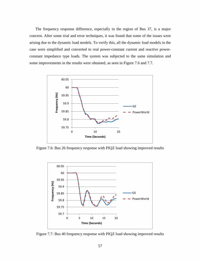
The frequency response difference, especially in the region of Bus 37, is a major
concern. After some trial and error techniques, it was found that some of the issues were
arising due to the dynamic load models. To verify this, all the dynamic load models in the
case were simplified and converted to real power-constant current and reactive power-
constant impedance type loads. The system was subjected to the same simulation and
some improvements in the results were obtained, as seen in Figure 7.6 and 7.7.
Figure 7.6: Bus 26 frequency response with PIQZ load showing improved results
Figure 7.7: Bus 40 frequency response with PIQZ load showing improved results
59.75
59.8
59.85
59.9
59.95
60
60.05
0 10 20
Freq
uenc
y (H
z)
Time (Seconds)
GE
PowerWorld
59.7
59.75
59.8
59.85
59.9
59.95
60
60.05
0 5 10 15 20
Freq
uenc
y (H
z)
Time (Seconds)
GE
PowerWorld
58
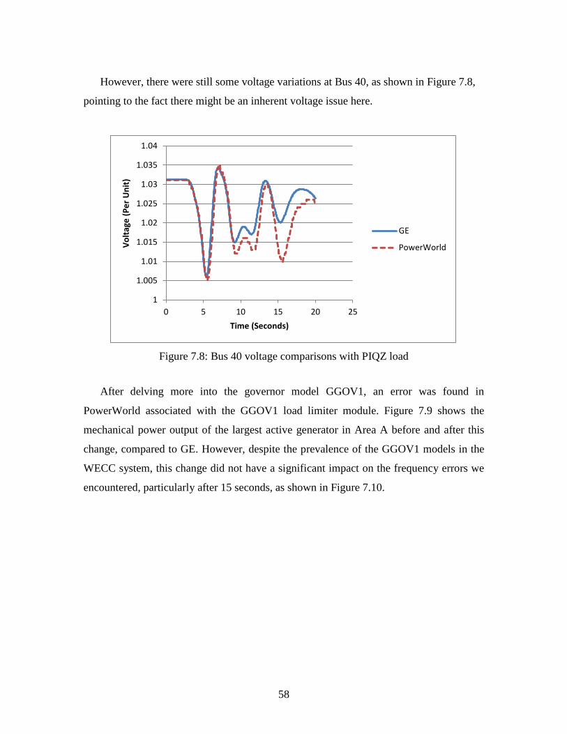
However, there were still some voltage variations at Bus 40, as shown in Figure 7.8,
pointing to the fact there might be an inherent voltage issue here.
Figure 7.8: Bus 40 voltage comparisons with PIQZ load
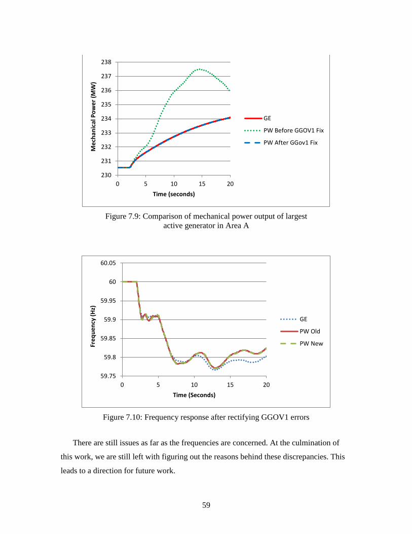
After delving more into the governor model GGOV1, an error was found in
PowerWorld associated with the GGOV1 load limiter module. Figure 7.9 shows the
mechanical power output of the largest active generator in Area A before and after this
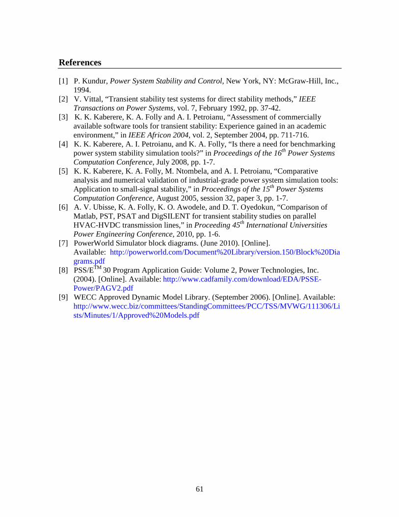
change, compared to GE. However, despite the prevalence of the GGOV1 models in the
WECC system, this change did not have a significant impact on the frequency errors we
encountered, particularly after 15 seconds, as shown in Figure 7.10.
1
1.005
1.01
1.015
1.02
1.025
1.03
1.035
1.04
0 5 10 15 20 25
Volta
ge (P
er U
nit)
Time (Seconds)
GE
PowerWorld
59
Figure 7.9: Comparison of mechanical power output of largest
active generator in Area A
Figure 7.10: Frequency response after rectifying GGOV1 errors
There are still issues as far as the frequencies are concerned. At the culmination of
this work, we are still left with figuring out the reasons behind these discrepancies. This
leads to a direction for future work.
230
231
232
233
234
235
236
237
238
0 5 10 15 20
Mec
hani
cal P
ower
(MW
)
Time (seconds)
GE
PW Before GGOV1 Fix
PW After GGov1 Fix
59.75
59.8
59.85
59.9
59.95
60
60.05
0 5 10 15 20
Freq
uenc
y (H
z)
Time (Seconds)
GE
PW Old
PW New

60
8. Summary and Directions for Future Work
We have presented and implemented a methodology to validate transient stability models
used in power systems. Although we focused on the generator and its associated models,
our methodology is scalable and can be used on systems of various sizes and for different
types of dynamic models such as load models.
From the vast differences in results obtained for essentially the same system and
similar models across different transient stability packages, this work also highlighted the
need for validation or software packages, transient stability models as well as results.
In Chapter 7, we concluded that we need to further investigate the reason for the
difference in frequency responses. There might potentially be more issues with some of
the softwares we used here that probably need more testing and analyses similar to the
ones charted out in this thesis
Another direction would be to try and automate these comparisons and the whole
validation process, both top-down and bottom-up, to handle the huge volumes of data and
get meaningful results quickly and efficiently.
Given the research thrust on increasing the penetration of renewables in the grid,
validation of dynamic models pertaining to wind turbines, solar models, etc., is also
another avenue that can and should be pursued
Additionally, a logical future step would be to validate these packages and their
simulation results with real-world data obtained from phasor measurement units (PMUs),
digital fault recorders (DFRs) and other sensing devices.
61
References
[1] P. Kundur, Power System Stability and Control, New York, NY: McGraw-Hill, Inc., 1994.
[2] V. Vittal, “Transient stability test systems for direct stability methods,” IEEE Transactions on Power Systems, vol. 7, February 1992, pp. 37-42.
[3] K. K. Kaberere, K. A. Folly and A. I. Petroianu, “Assessment of commercially available software tools for transient stability: Experience gained in an academic environment,” in IEEE Africon 2004, vol. 2, September 2004, pp. 711-716.
[4] K. K. Kaberere, A. I. Petroianu, and K. A. Folly, “Is there a need for benchmarking power system stability simulation tools?” in Proceedings of the 16th Power Systems Computation Conference, July 2008, pp. 1-7.
[5] K. K. Kaberere, K. A. Folly, M. Ntombela, and A. I. Petroianu, “Comparative analysis and numerical validation of industrial-grade power system simulation tools: Application to small-signal stability,” in Proceedings of the 15th Power Systems Computation Conference, August 2005, session 32, paper 3, pp. 1-7.
[6] A. V. Ubisse, K. A. Folly, K. O. Awodele, and D. T. Oyedokun, “Comparison of Matlab, PST, PSAT and DigSILENT for transient stability studies on parallel HVAC-HVDC transmission lines,” in Proceeding 45th International Universities Power Engineering Conference, 2010, pp. 1-6.
[7] PowerWorld Simulator block diagrams. (June 2010). [Online]. Available: http://powerworld.com/Document%20Library/version.150/Block%20Diagrams.pdf
[8] PSS/ETM 30 Program Application Guide: Volume 2, Power Technologies, Inc. (2004). [Online]. Available: http://www.cadfamily.com/download/EDA/PSSE-Power/PAGV2.pdf
[9] WECC Approved Dynamic Model Library. (September 2006). [Online]. Available: http://www.wecc.biz/committees/StandingCommittees/PCC/TSS/MVWG/111306/Lists/Minutes/1/Approved%20Models.pdf