Utilizing Wireless-based Data Collection Units for Automated Vehicle Movement Data Collection
139
Transcript of Utilizing Wireless-based Data Collection Units for Automated Vehicle Movement Data Collection

AN ABSTRACT OF THE DISSERTATION OF
Amirali Saeedi for the degree of Doctor of Philosophy in
Industrial Engineering presented on February 22 2013
Title Utilizing Wireless-based Data Collection Units for Automated Vehicle
Movement Data Collection
Abstract approved ______________________________________________ David S Kim
There are many different types of automatic data collection technologies that have
been used in transportation system applications such as pneumatic tubes radar video
cameras inductive loops detectors wireless toll tags and global positioning systems
(GPS) Nevertheless there are still multiple examples of important and helpful
transportation system data that still require manual data collection In this research
the automatic transportation system data collection capabilities are expanded by
enhancements in the use of wireless communications technology
In recent years smartphones and electronic peripherals with wireless communication
capabilities have become very popular Many of these electronic devices include a
Bluetooth or Wi-Fi wireless radio whose presence in a vehicle can be used as a
vehicle identifier With wireless on-board devices available now and in the future
this research explores how roadside data collection units (DCUs) communicating with
on-board devices can be used for the automated data collection of important road
system data such as intersection performance data
To this end two approaches for wirelessly collecting vehicle movement over a short
road segment were explored One approach utilized the collection and triangulation of
wireless signal strength data and demonstrated the capabilities and limitations of this
approach The second approach focused on developing methods for utilizing wireless
signal strength data for vehicle point detection and identification
The vehicle point detection methods developed were applied to collect travel time
data over signalized arterial roads and to collect intersection delay data for a three
way stop controlled intersection The results from these case studies indicate a
significant advantage in the proposed data collection system over the existing data
collection approaches presented in the literature
copyCopyright by Amirali Saeedi
February 22 2013
All Rights Reserved
Utilizing Wireless-based Data Collection Units for Automated Vehicle Movement
Data Collection
by
Amirali Saeedi
A DISSERTATION
submitted to
Oregon State University
in partial fulfillment of
the requirements for the
degree of
Doctor of Philosophy
Presented February 22 2013
Commencement June 2013
Doctor of Philosophy dissertation of Amirali Saeedi presented on
February 22 2013
APPROVED
Major Professor representing Industrial Engineering
Head of the School of Mechanical Industrial and Manufacturing Engineering
Dean of the Graduate School
I understand that my dissertation will become part of the permanent collection of
Oregon State University libraries My signature below authorizes release of my
dissertation to any reader upon request
Amirali Saeedi Author
ACKNOWLEDGEMENTS
I would especially like to thank my advisors Dr David S Kim and Dr J David
Porter for guiding me through this research with excellent patience and for the given
encouragements I would also like to thank my committee members Dr Toni Doolen
Dr Karen Dixon Dr David Hurwitz and Dr Scott Leavengood for their suggestions
and for reviewing this work
This work has received major benefits from discussions with other graduate students
in the Industrial Engineering Department at OSU among them Dr Sejoon Park
TABLE OF CONTENTS
Page
1 INTRODUCTION 1
11 RESEARCH MOTIVATION 1
12 RESEARCH OBJECTIVES 3
13 RESEARCH CHALLENGES 6
14 CONNECTION TO VEHICLE-TO-INFRASTRUCTURE RESEARCH 8
15 RESEARCH CONTRIBUTION 8
16 THESIS ORGANIZATION 10
2 LITERATURE REVIEW 11
21 TRAFFIC MEASURES OF EFFECTIVENESS 11
211 INTERSECTION PERFORMANCE MEASURES 15
22 AUTOMATIC DATA COLLECTION TECHNOLOGIES 17
221 EXISTING TRAVEL DATA COLLECTION SYSTEMS 21
23 BLUETOOTH TECHNOLOGY 25
231 BLUETOOTH-BASED DATA COLLECTION SYSTEMS 25 232 BLUETOOTH SIGNAL DISTANCE-SIGNAL STRENGTH RELATIONSHIP 29
24 CONNECTED VEHICLE RESEARCH INITIATIVE 30
3 METHODOLOGY 34
31 BLUETOOTH TECHNOLOGY 35
32 TRILATERATION APPROACH TO ESTIMATE VEHICLE MOVEMENT37
321 BLUETOOTH SIGNAL STRENGTH ACQUISITION 38 322 ESTIMATING DISTANCE FROM RSSI 39 323 PARTICLE SWARM OPTIMIZATION 43 324 SIGNAL LOCALIZATION APPROACHES 46
TABLE OF CONTENTS (Continued)
Page
325 TRILATERATION STUDY TO DEVELP A SIGNAL PROPAGATION MODEL 49 326 FITTING THE ENVIRONMENT POWER DECAY FACTOR 52 327 ACCURACY ASSESSMENT 54 328 CONCLUSIONS AND LIMITATIONS 55
33 VEHICLE POINT DETECTION SYSTEM 56
331 VEHICULAR MOVEMENTS NEAR A DATA COLLECTION UNIT AND THE RSSI-DISTANCE RELATIONSHIP 57 332 POINT DETECTION ALGORITHM 61 333 VALIDATION EXPERIMENTS 68
4 APPLICATION CASE STUDIES 80
41 TRAVEL TIME STUDY 80
411 GENERATION OF TRAVEL TIME SAMPLES USING MAC ADDRESS DATA 82 412 TRAVEL TIME SAMPLE GENERATION SUPPLEMENTED WITH RSSI DATA 83
42 INTERSECTION PERFORMANCE 88
421 INTERSECTION TEST SETUP 90 422 TEST RESULTS AND CONCLUSIONS 91
5 CONCLUSIONS 95
BIBLIOGRAPHY 98
APPENDICES 104
APPENDIX A BLUETOOTH INQUIRY PROCEDURE 105
APPENDIX B TRILATERATION ALGORITHM CODE 109
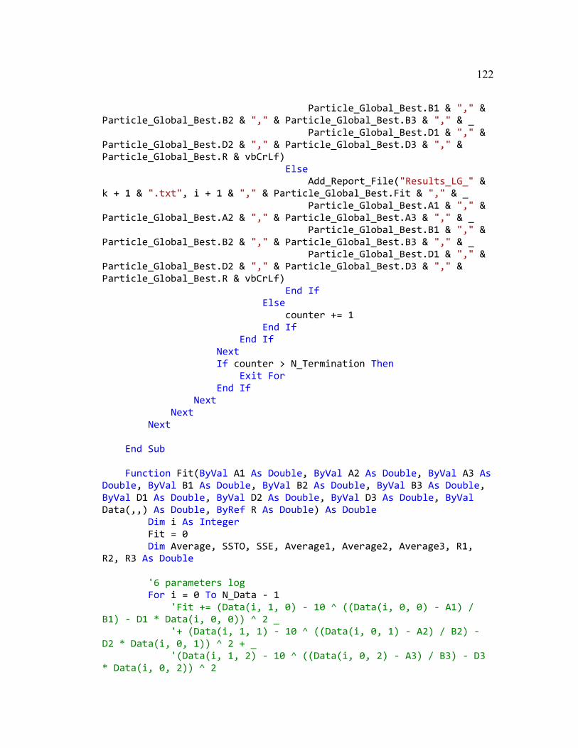
APPENDIX C PARTICLE SWARM OPTIMIZATION ALGORITHM IN VISUAL BASIC 113
LIST OF FIGURES
Figure Page
11 A Set of Three Wireless DCUs Installed at a Signalized Intersection 5
12 Schematic Representation of Bluetooth DCU Detection Range 7
31 Intersection of Three Circles at a Single Point 48
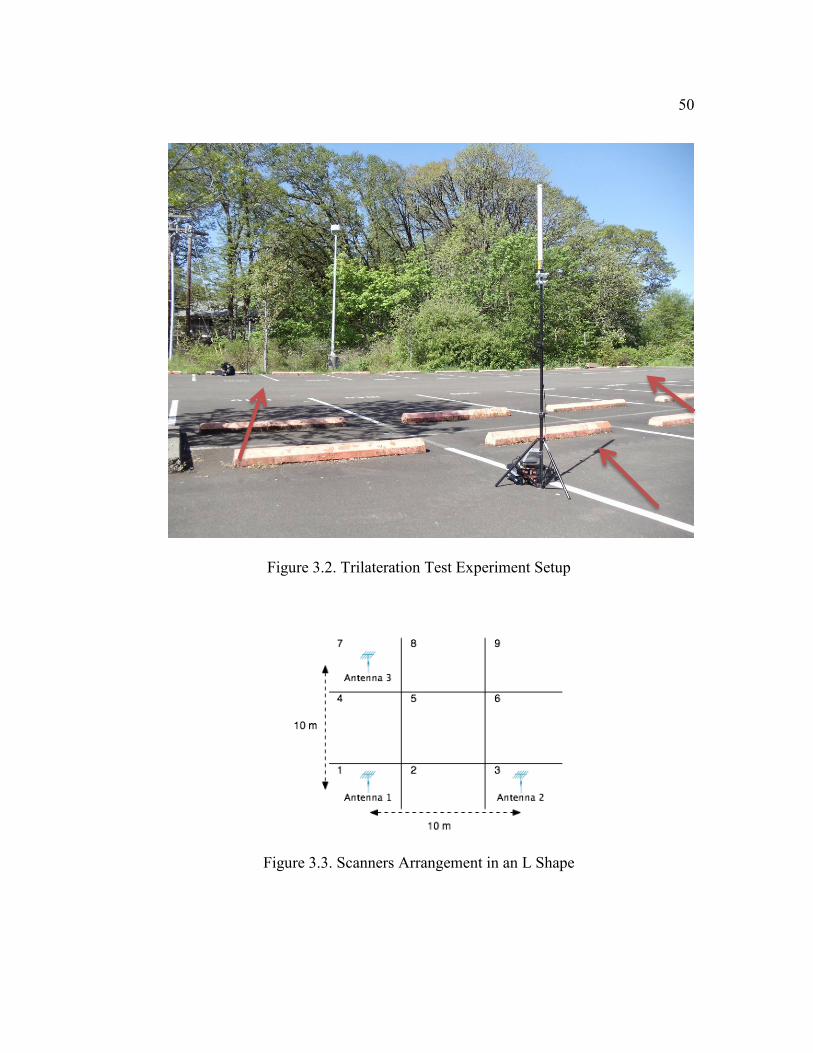
32 Trilateration Test Experiment Setup 50
33 Scanners Arrangement in an L Shape 50
34 Error Comparisons for Estimated Distances Using the Developed Signal Propagation Model for Both Test Cellphones 53
35 Highlighted Example of a Through Pass RSSI and Distance Sample Data 59
36 Highlighted Example of a Stop Far From Stop Line RSSI and Distance Sample Data 59
37 Highlighted Example of a Stop Near Stop Line RSSI and Distance Sample Data 60
38 Multiple detections within the DCUs detection zone 63
39 Schematic representation of multiple detections in a single trip forming a group 65
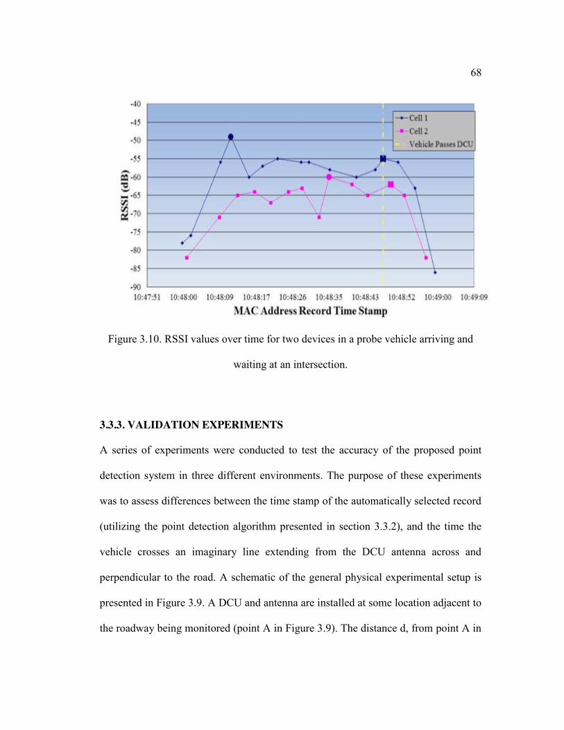
310 RSSI values over time for two devices in a probe vehicle arriving and waiting at an intersection 68
311 DCU installation on Camp Adair Road Benton County 71
312 Histogram of the difference between the time the probe vehicle passed the DCU on Camp Adair Road and the MAC address record with the highest RSSI 71
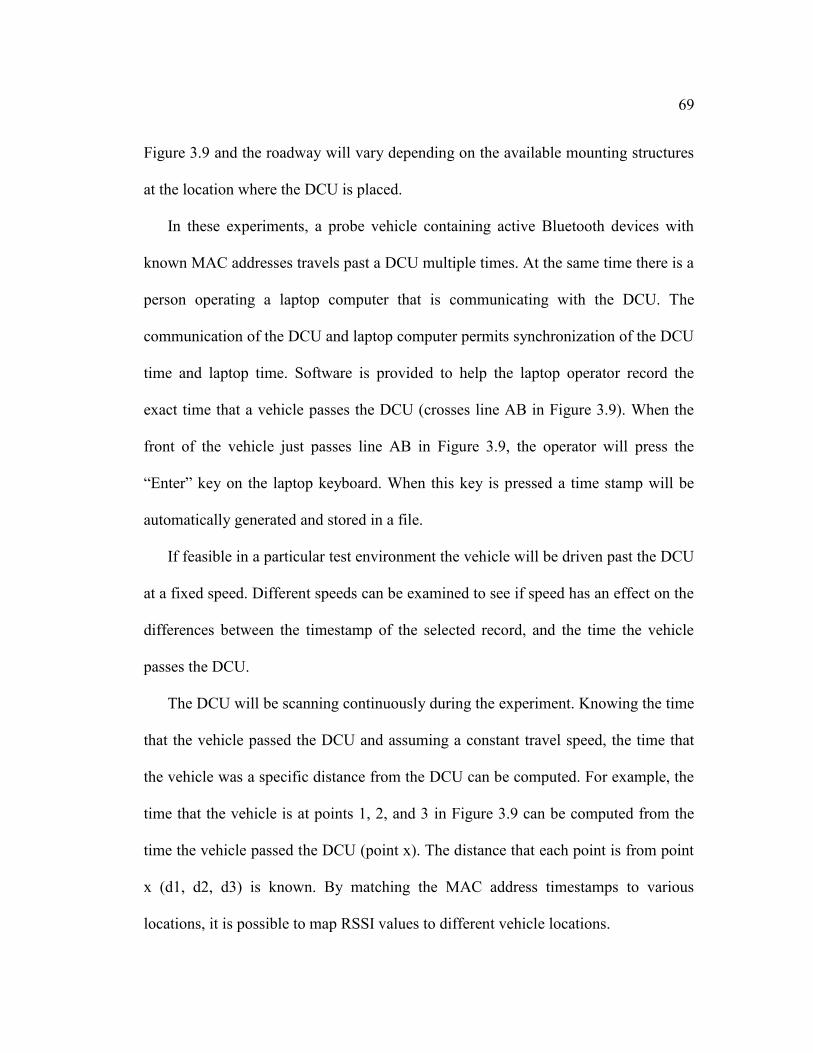
313 DCU Location on Wallace Road Salem Oregon 73
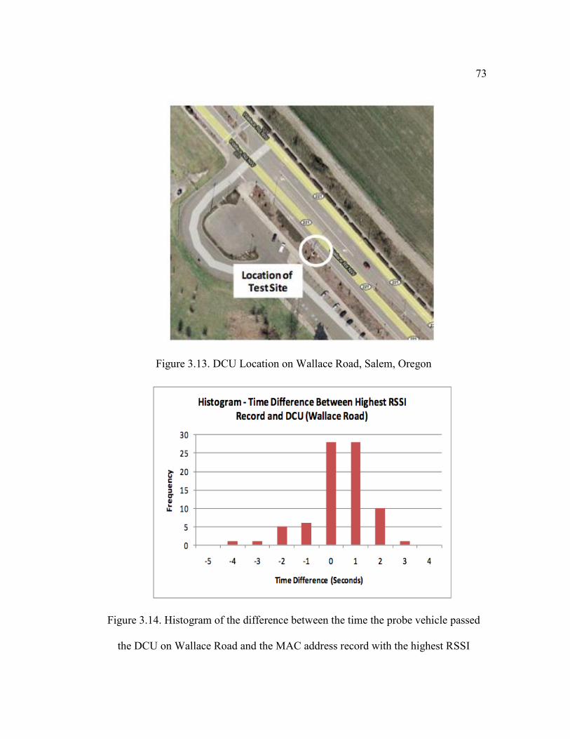
314 Histogram of the difference between the time the probe vehicle passed the DCU on Wallace Road and the MAC address record with the highest RSSI 73
315 Southernmost DCU locations on Highway 99W Tigard Oregon 74
316 Southernmost DCU locations on Highway 99W Tigard Oregon 75
LIST OF FIGURES (Continued)
Figure Page
317 Histogram of the difference between the time the probe vehicle passed DCU 12 on Highway 99W and the MAC address record with the highest RSSI 77
318 Histogram of accuracy of the time stamp before the RSSI values rapidly decrease 79
41 Location of Bluetooth DCUs on Highway 99W (Tigard OR) 82
42 Test Setup Utilized in the Intersection Control Delay Experiment 89
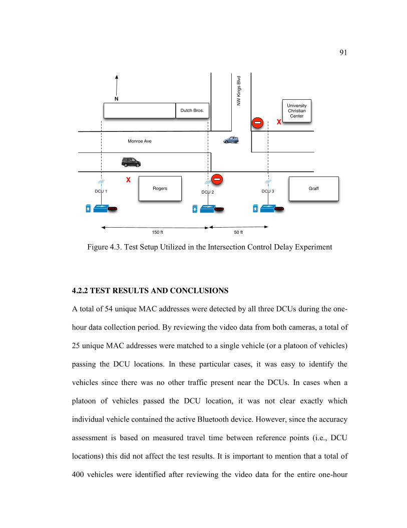
43 Test Setup Utilized in the Intersection Control Delay Experiment 91
LIST OF TABLES
Table Page
21 Selected arterial performance measures 13
22 Most Common Automated Data Collection Technologies Used in Transportation Applications 18
31 Bluetooth Classifications 36
32 Random locations selected for Test Cell Phone 1 51
33 Signal Propagation Model Accuracy Test Results 55
34 Sample of MAC Address Data from an Installed Bluetooth DCU 64
41 Cell Phone 1 Sample Probe Vehicle Test Results for the Road Segment between Johnson St and the 217 NB Ramp 85
42 Average Absolute Travel Time Sample Errors in Seconds for Different Travel Time Calculation Approaches 86
43 The Volume Of Travel Time Samples Generated Compared To Traffic Volume 88
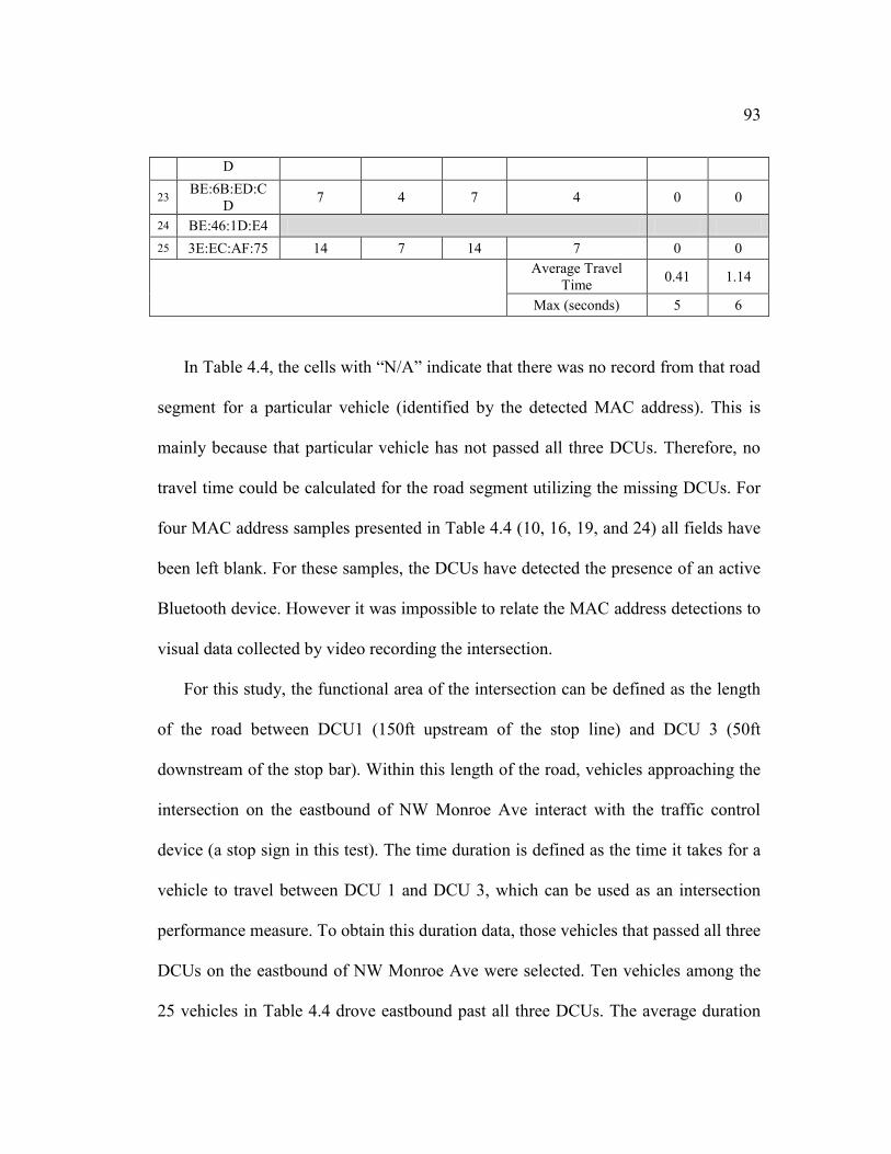
44 Summary Results from the Intersection Delay Study 92
A1 Discovery probability of Bluetooth devices in relation to inquiry time (Nicolai amp Kenn 2007) 108
DEDICATION
To my parents for their unconditional love and endless patience
1 INTRODUCTION
There are many different types of automatic data collection technologies that have
been used in transportation system applications such as pneumatic tubes radar video
cameras inductive loops detectors wireless toll tags and global positioning system
(GPS) Nevertheless there are many types of transportation system data that still
require manual data collection In this research the capabilities of automatic
transportation system data collection are expanded by enhancements in the use of
wireless communications technology The introduction to this research will begin
with an overview of the motivating transportation system data collection application
for which automation will be beneficial This will be followed by a specification of
the research objectives and an overview of the research approach This introductory
chapter will conclude with a discussion of the research contributions presented and
the organization of this thesis
11 RESEARCH MOTIVATION
Intersections in urban and rural highway networks have a significant role on the
operation and performance of the traffic system since the performance of an
intersection controls the performance of the roads meeting at that intersection
Intersections can be bottlenecks in a road network with respect to throughput
affecting the capacity of the road system and its efficiency (as measured by travel
2
times) which may result in an impact on traffic congestion and safety The effect of
intersections on road network performance has been studied in previous research
(Ibrahim et al 2008 Sharma amp Swami 2010) Accordingly there has been research
directed at intersection design and control to increase capacity and provide high levels
of safety (Pickrell amp Neumann 2001) While the importance of intersections on the
performance of the traffic system and on safety has been recognized the acquisition
of intersection performance data still relies on manual data collection methods
Although more advanced automated methods are being tested but they are not
common practice yet There exist a number of different intersection performance
measures However the 2010 Highway Capacity Manual (Transportation Research
Board 2010) designates average control delay as the primary performance measure
for signalized intersections Control delay is defined as the total delay a vehicle
experiences due to interaction with the traffic control device at the intersection It
includes delay due to deceleration stopping and acceleration There are no currently
available low-cost automated data collection methods that can be utilized to collect
data to estimate control delay
In addition to intersections there are a variety of road segments that are ldquoareas of
interestrdquo for engineers where manual data collection is required These road segments
usually have some performance functional or geometric characteristics that require
engineers to conduct on-site data collection studies to investigate the cause for
existing issues or to predict vulnerable situations (eg for future developments)
3
Generally the criteria listed below can help to identify areas of interest for
transportation engineers
- Performance criteria Highly congested routes intersections with excessive
delays and corridors with high accident rates are main areas of interest For
these situations road segment data can help engineers to identify solutions to
the problems
- Functional criteria Some road segments may have been assigned a unique
functionality that distinguishes them from other road segments Airport roads
industrial roads interstate highways and roads located on evacuation plans
are main examples of this category (Kirby amp Pickett 2001) Road segment
data can be used to determine road segment performance for specific
functions
- Geometric criteria Sometimes a physical factor can change or affect (usually
for a short period of time) the normal functionality of a road segment
Examples could be construction zones accident sites or roads adjacent to an
attraction (high demand) center (US Department of Transportation 2008)
12 RESEARCH OBJECTIVES
In recent years smartphones and electronic peripherals with wireless communication
capabilities have become very popular Many of these electronic devices include a
Bluetooth or Wi-Fi wireless radio whose presence in a vehicle can be used as a
vehicle identifier In the future it is envisioned that vehicles will be equipped with
4
on-board Dedicated Short Range Communication (DSRC) devices With wireless on-
board devices available now and in the future this research will explore how roadside
data collection units (DCUs) communicating with on-board devices can be used to
address the lack of automated data collection for important road system components
such as intersections
The objective of this research is to explore the capabilities of wireless radio
frequency technology with respect to automated vehicle data collection An
exploration of collecting vehicle movement data utilizing triangulation of wireless
signal data is conducted and demonstrates the capabilities and limitations of this
approach The research then focuses on developing the knowledge of how wireless
radio frequency technology can be utilized to provide automated vehicle point
detection and identification capability In this research vehicle point detection refers
to the determination of the time a traveling vehicle just crosses a specific line crossing
a road The wireless vehicle point detection and identification capability can then be
used to collect road segment data from which performance measures such as control
delay (and other measures) can be estimated The purpose of this study is to utilize
wireless technologies to collect vehicle movement data and the focus is not on
obtaining performance measures However to validate the wireless data collection
system proposed in this study the application of the proposed system in obtaining
travel time data over signalized arterial roads and intersection delay were
demonstrated through two case studies Estimating these measures assumes that a
DCU 1 DCU 2 DCU 3
5
sufficient number of travelling vehicles are equipped or contain the wireless
technology that can be wirelessly detected and used as a vehicle identifier
For the intersection control delay application multiple wireless DCUs can be
placed at known distances along a road both before and after an intersection as
depicted in Figure 11 By using multiple DCUs data on vehicle position over time
may be collected for those vehicles containing detectable wireless devices This data
can be used to compute performance measures such as travel times through areas of
interest and can be used to show how congestion builds over time in specific areas
due to non-recurring events
Figure 11 A Set of Three Wireless DCUs Installed at a Signalized Intersection
6
Compared to other technologies that have both vehicle point detection and
identification capabilities (eg video and GPS technology) wireless data collection
units are inexpensive and may be deployed as portable or permanently installed
DCUs Permanently installed DCUs may also be connected to central traffic data
management systems through an existing network infrastructure or through wireless
technologies During this study the concept has been tested through both temporary
and permanent deployment of the wireless-based data collection units
13 RESEARCH CHALLENGES
One characteristic of wireless data collection systems is that they typically have a
large detection range At a roadside DCU a vehicle containing a discoverable
Bluetooth device is often detected multiple times as it travels within the antenna
coverage area of the DCU as depicted in Figure 12 Each detection of the same
device in a vehicle will have a different time stamp When utilized for travel time data
collection this characteristic of vehicle data collected using Bluetooth technology has
been widely acknowledged by several researchers (Van Boxel et al 2011 Tsubota et
al 2011) as the main cause for travel time sample inaccuracy Due to these spatial
errors associated with data collected by Bluetooth DCUs researchers believe that
Bluetooth wireless data collection is not precise enough for travel time data collection
on shorter arterial segments (Saito amp Forbush 2011 Wasson et al 2008) The spatial
errors associated with wireless data collection is the main challenge addressed in this
research
7
Figure 12 Schematic Representation of Bluetooth DCU Detection Range
To develop the point detection capability with wireless DCUs received signal
strength indicator (RSSI) data is utilized Within the Bluetooth technology
communication protocol RSSI data are available at the same time devices are
detected In other wireless platforms such as Wi-Fi ZigBee and DSRC the RSSI
data are also available both during the inquiry process and once a connection (ie
pairing) of devices has been established The key feature of RSSI data that helps
develop point detection capability is the correlation of RSSI values with distance The
basic idea that is expanded upon in this research is that when a vehicle is detected
multiple times as it travels through the DCU antenna coverage area RSSI data can be
8
utilized to identify the detection that corresponds to when the vehicle was the closest
to the DCU
14 CONNECTION TO VEHICLE-TO-INFRASTRUCTURE RESEARCH
The ideas proposed in this research are implemented as a wireless-based Vehicle-To-
Infrastructure (V2I) data collection system that utilizes an existing infrastructure
based on the Bluetooth wireless communications protocol The focus on Bluetooth
technology is due to the presence of many detectable Bluetooth devices that can
currently be found in traveling vehicles Thus research findings can be tested and
utilized on actual roads with varying traffic characteristics Accordingly this research
can also provide more near-term data collection solutions for the types of applications
discussed earlier The research developments will also contribute to the Connected
Vehicle Research initiative for V2I communications (US Department of
Transportation 2010) In the Connected Vehicle Research federal initiative DSRC
wireless technology operating in 59 GHz band is utilized instead of Bluetooth which
operates at 24 GHz Nevertheless the approach and methods developed in this
research are applicable to other wireless technologies and in particular to DSRC
15 RESEARCH CONTRIBUTION
In this research the limits of using a single wireless roadside DCU as a point
detection device for vehicles containing a detectable wireless device are explored
9
The spatial errors associated with wireless data collection from moving vehicles is the
main challenge addressed in this research The approach explored to address these
spatial errors is the acquisition and processing of RSSI data which can be obtained at
the same time device identification occurs The resulting point detection precision
realized is sufficient for a variety of road segment data collection applications This is
demonstrated using Bluetooth wireless technology Multiple DCUs were utilized as
point detection units at a three-way intersection to collect vehicle movement data
Results obtained from the wireless data collection were compared to ldquoground truthrdquo
data obtained from video recordings
Although Bluetooth technology was used as the implementation platform the
approach and principles utilized are applicable to other wireless technologies In
particular the approach of utilizing and processing RSSI data is also applicable to
DSRC wireless technology
The results and approach developed in this research and implemented in
Bluetooth offers a current solution for a low-cost automated data collection system
that is capable of providing data that is unavailable through most current automatic
data collection techniques (with the exception of video image processing and GPS
probe vehicle data collection ndash neither of which is low cost) Data from multiple
Bluetooth-based DCUs can collect sufficiently precise vehicle movement data over
many types of road segments for a variety of purposes With respect to intersections
there are multiple topics in practice and research that would benefit from the
availability of such data Some of these topics are reducing fuel consumption and
10
emissions through traffic signal strategies active traffic management for signalized
networks assessing signal timing and control strategies and intersection performance
and travel time reliability
16 THESIS ORGANIZATION
In the next chapter a summary of the literature relevant to this research is presented
Next the methodologies investigated in this research are explained in detail
including two wireless-based traffic data collection methods A series of test
experiments are conducted to validate the methods proposed in this research and a
summary of the results of these experiments is provided Finally a few examples of
the real-world applications of the proposed techniques are presented
11
2 LITERATURE REVIEW
In this chapter a review of the literature concerning modern traffic data collection
technologies is provided This review focuses on advanced non-intrusive traffic data
collection technologies that do not interrupt traffic during installation andor
operation
First an introduction of traffic performance measures and more specifically
measures of effectiveness applicable to intersections is presented Next a summary of
existing automatic data collection systems is presented with more detail on travel time
and other wireless data collection systems currently in practice Finally a summary of
the connected vehicle research initiative is presented and its relevance to this study is
briefly discussed
21 TRAFFIC MEASURES OF EFFECTIVENESS
The Federal Highway Administration (FHWA) defines a performance measure as the
ldquouse of statistical evidence to determine the progress towards specific defined
operational objectivesrdquo A performance measure provides a basic understanding of
whether different aspects of the transportation system performance are getting better
or worse (Balke et al 2005) For example arterial performance measures obtained
over time can help transportation managers and operators to better evaluate the
effectiveness of signal timing plans and other operational improvements In the long
12
run planning agencies would be able to monitor the arterial network and understand
the effects of changing land uses (Bertini et al 2001)
According to Schrank et al (2007) the public motoring cost during traffic
congestion delay is worth more than a billion dollars in extra travel time extra energy
consumption and extra environmental impacts Signalized intersections are usually
designed with the primary emphasis on minimizing delay Traffic signals when
implemented properly can reduce delay and accidents and improve the quality of
traffic movement (Courage amp Parapar 1975) Signal timing strategies include the
minimization of stops delays fuel consumption and air pollution emissions and the
maximization of progressive movement through a system (Li et al 2004) Improving
signal timing reduces fuel consumption and emissions hence improving air quality
Signal retiming is a process that optimizes the operation of signalized
intersections through a variety of low-cost improvements including the development
and implementation of new signal timing parameters phasing sequences improved
control strategies and occasionally minor roadway improvements Sunkari (2004)
has summarized a comprehensive list of successful examples for signal retiming
projects demonstrating a significant amount of savings in delay time and fuel
consumption at intersections
Researchers use a wide variety of traffic characteristics and performance
measures to study traffic problems For intersections agencies use different
performance measures to quantify the efficiency of roadway systems and evaluate the
movement operations Typical intersection data collection has been limited to
13
volume occupancy travel time and average speed and the assessment has been
conducted off-line (US Department of Transportation 2010) In other words the
researcher collected the data in the field and returned to the office for further data
analysis Therefore there was always a time lag between when the observation was
conducted and when the analysis was completed Recently a trend toward online data
collection techniques has been raised in studies related to roadway and intersection
operations performance (Balke et al 2005 US Department of Transportation 2010
Bonneson amp Abbas 2002) By using real-time traffic data drivers can be kept
updated about the traffic conditions to make their driving safer and more efficient
Shaw (2003) has conducted an extensive survey on arterial performance measures In
his study an overview of the most common arterial performance measures is
presented These measures are summarized in Table 21
Table 21 Selected arterial performance measures
Metric Metric
1 Maximum Speed 10 Queue Length
2 Average Speed 11 Platoon Ratio1
3 Speed Index2 12 Number of Stops
1 Ratio of platoon miles traveled to vehicle miles traveled 2 A ratio that is calculated by dividing a roadway segmentacutes average observed travel speed by the posted speed limit for that segment
14
Metric Metric
4 Density 13 Signal Failure
5 Travel Time 14 Duration of Congestion
6 Travel Time Variance 15 Number of Incidents
7 Average Delay 16 Incidents Duration
8 Maximum Delay 17 Nonrecurring Delay
9 Level of Service (LOS)3 18 Emissions
The traffic performance measures presented in Table 21 are among the most
common metrics used to support decisions that may results in changes to the
transportation system Many transportation agencies have begun to introduce explicit
transportation system performance measures into their policies planning and
programming activities (Pickrell amp Neumann 2001) Depending on the area of use
some performance measures may be more explanatory and useful than others In
addition the metrics presented in Table 21 can be further customized for different
areas of interest Travel time speed and volume are major arterial performance
measures (Wolfe et al 2001) Travel time and volume data collection based on the
reading of time-stamped media access control (MAC) addresses from Bluetooth
3 A performance measure used by traffic engineers to determine the effectiveness of elements of a transportation system
15
enabled devices has been in use for several years (Wasson et al 2008) A basic setup
to collect travel time data via Bluetooth includes a reader unit and an antenna These
two components collectively are referred to as the data collection unit (DCU) With
DCUs placed at different locations along a road segment computing the time-stamp
differences for the same MAC address read at each DCU could generate travel time
samples
211 INTERSECTION PERFORMANCE MEASURES
Engineers and researchers tend to use specific performance measures for different
traffic infrastructures as they are more descriptive to those particular systems In this
section a series of intersection performance measures are explained These measures
are commonly used in studies focused on arterial roads and intersections
As a performance measure delay plays a critical role when evaluating service
level at signalized and un-signalized intersections The average time that vehicles
spend at an intersection is directly related to the average delay for that particular
intersection The 2010 Highway Capacity Manual (HCM) designates average control
delay as the primary performance measure for signalized intersections
(Transportation Research Board 2010) Control delay is used in traffic signal timing
as well as to obtain the level of service (a common intersection measure of
performance) for a particular intersection The Highway Capacity Manual defines
level of service for signalized and un-signalized intersections as a function of the
16
average vehicle control delay This measure is popular since it can be presented to
people without any knowledge in transportation engineering
Two major delay types are defined for intersections stopped time delay and
control delay Stopped delay is defined as the time a vehicle is stopped at an
intersection Control delay is defined as the total delay due to the interaction of
vehicles with the type of control utilized at the intersection and includes deceleration
delay stopped delay and acceleration delay (Quiroga amp Bullock 1998)
Theoretically control delay is measured by comparison with the uncontrolled
condition ie the difference between the travel time that would have occurred in the
absence of the intersection control and the travel time that results because of the
presence of the intersection control Existing techniques for measuring control delay
are inaccurate and time-consuming Therefore control delay is rarely measured
Acceleration and deceleration time and distance data or vehicle trajectories are
other important intersection data and are mainly related to signal timing
performance and safety aspects of the intersection design Acceleration and
deceleration distances and times associated with speed change cycles (stop start and
slow down speed up maneuvers) under normal driving conditions is essential for the
analysis of determining geometric stopped and queuing components of intersection
control delay Vehicle trajectory information is also essential for development and
calibration of simulation models the analysis of operating cost fuel consumption and
pollutant emissions Many efforts have been summarized in the literature to model
acceleration and deceleration profiles (Akcelik amp Besley 2001 Bennett 1994)
17
Unfortunately due to the complexity of such maneuvers the literature on vehicle
trajectories has been very limited Since direct observation and measurement of
vehicle trajectories tend to be inaccurate and impractical the developed models have
been limited to historical or simulation data
In this research the data collection efforts and proposed methodologies are
mainly focused on intersection delay vehicular speed and travel times at signalized
arterial roads Travel time and delay are intuitive performance measures
understandable for both engineers and public road users which can provide valuable
information on the quality of roadway system
22 AUTOMATIC DATA COLLECTION TECHNOLOGIES
To frame the relevance of the proposed research a review of the current automated
traffic data collection technologies and a review of the relevant research literature
were conducted Table 22 summarizes the most common automatic data collection
techniques used in transportation applications
18
Table 22 Most Common Automated Data Collection Technologies Used in Transportation Applications
bull Technology bull Pros bull Cons
Inductive Loop
bull Mature well understood technology
bull Large experience base
bull Provides basic traffic parameters (eg volume presence
occupancy speed headway and gap)
bull Insensitive to inclement weather such as rain fog and snow
bull Provides best accuracy for count data as compared with other
commonly used techniques
bull Common standard for obtaining accurate occupancy
measurements
bull High frequency excitation models provide classification data
bull Installation requires pavement cut
bull Improper installation decreases pavement life
bull Installation and maintenance require lane closure
bull Wire loops subject to stresses of traffic and temperature
bull Multiple detectors usually required to monitor a location
bull Detection accuracy may decrease when design requires
detection of a large variety of vehicle classes
bull Destroyed by utility cuts or pavement milling operations
Microwave Radar
bull Typically insensitive to inclement weather at the relatively short
ranges encountered in traffic management applications
- Direct measurement of speed
- Multiple lane operation available
bull Continuous Wave (CW) Doppler sensors cannot detect
stopped vehicles
19
(Continued)
TECHNOLOGY PROS CONS
Infrared
(Laser Radar)
bull Transmits multiple beams for accurate measurement of vehicle
position speed and class
bull Multiple-lane operation available
bull Operation may be affected by fog when visibility is less
than ~6 m (20 ft) or blowing snow is present
bull Installation and maintenance including periodic lens
cleaning require lane closure
Ultrasonic
bull Multiple-lane operation available
bull Capable of over height vehicle detection
bull Large Japanese experience base
bull Environmental conditions such as temperature change and
extreme air turbulence can affect performance
bull Large pulse repetition periods may degrade occupancy
measurement on freeways with vehicles traveling at
moderate to high speeds
Bluetooth
bull Multiple-lane operation
bull Can operate during night time and all weather conditions
bull Non-intrusive
bull Installation and maintenance does not need to interrupt the traffic
bull Cannot capture the entire traffic Can only sample the
vehicles with active an Bluetooth device onboard
bull Spatial errors
20
(Continued)
TECHNOLOGY PROS CONS
Video Image
Processor
bull Monitors multiple lanes and multiple detection zoneslanes
bull Easy to add and modify detection zones
bull Rich array of data available
bull Provides wide area detection when information gathered at one
camera location can be linked to another
bull Installation and maintenance including periodic lens
cleaning require lane closure when camera is mounted over
roadway (lane closure may not be required when camera is
mounted at side of roadway)
bull Performance affected by inclement weather such as fog
rain and snow vehicle shadows vehicle projection into
adjacent lanes occlusion day-to-night transition
vehicleroad contrast and water salt grime icicles and
cobwebs on camera lens
bull Requires15-to21-m(50-to70-ft) camera mounting height (in
a side-mounting configuration) for optimum presence
detection and speed measurement
bull Some models susceptible to camera motion caused by
strong winds or vibration of camera mounting structure
21
As can be seen from the information in Table 22 there are major limitations with
existing technologies in terms of cost flexibility and richness of data that the
technology offers Additionally automatic data collection technologies and
particularly wireless-based systems tend to generate a lot of data However the
output data is not always accurate and useful Therefore to get reliable results from
any automatic data collection system it is necessary to take extra steps before and
after data collection occurs to guarantee the acquisition of quality data For the
purpose of travel time data collection it is necessary to use a series of filtering
techniques to eliminate outlier input data and apply prediction and smoothing
techniques to generate reliable travel time estimates
Among all the existing data collection systems this research is primarily focused
on travel time data collection systems In the next section an overview of the existing
travel data collection systems is presented
221 EXISTING TRAVEL DATA COLLECTION SYSTEMS
Travel time data is one of the most important traffic measures of performance A
wide range of automatic travel time data collection systems have been in practice for
a long time In this section an overview of these technologies is presented
The TransGuide traffic management center monitors traffic operations on a
network of freeways and major arterial streets covering most of the metropolitan area
of San Antonio TX One of the main components of the monitoring system is a series
of sensors (mainly loop detector pairs and sonic detectors) spaced roughly 05 miles
22
apart that provide the capability to measure point speeds Based on these point
speeds the system estimates travel times to specific landmarks and displays the
estimated travel times on dynamic message signs (DMSs) located approximately
every 2 to 3 miles For each pair of adjacent detector stations the system determines
the lowest of the two detector station speeds and assigns that speed to the road
segment that connects the adjacent detector stations The system converts each partial
road segment speed into an equivalent travel time and adds all of the partial segment
travel times to produce an estimate of the total travel time between the DMS location
and the major interchange
Besides TransGuide there are three other major traffic data detection and
archiving programs in Texas TransVista in El Paso TransStar in Houston and
DalTrans in Dallas The TransVista system uses a combination of point loop detectors
and fifty-five cameras to monitor sections of the roadway DMSs and lane control
signs are used to disseminate information about freeway conditions to the travelers
The freeway sections visible through the cameras can be accessed on the Internet
(PBSampJ 2001)
The TransStar system in Houston uses Automatic Vehicle Identification (AVI) to
monitor freeway traffic and disseminate information through popular media outlets
such as radio television and DMSs Primary information transmitted are travel time
estimates and speed data Vehicles with transponders are used as probes AVI readers
are installed along freeways to detect when the probe vehicles pass the point of
23
installation The time difference between detection of a probe vehicle at successive
AVI reader locations is used to arrive at travel time estimates and speed
The DalTransTransVision system in Dallas uses a combination of loop detectors
and closed circuit cameras to provide information about incidents lane closures and
speeds in the Dallas and Fort Worth areas The information is provided to the public
using DMSs or it can be accessed on the Internet
The Florida Department of Transportation (DOT) collects real-time data on a 40-
mile segment on the I-4 corridor near Orlando using loop detectors (coupled as dual-
loops) A nonlinear time series model developed at the University of Central Florida
was used to predict travel times This forecasted travel time information was
transmitted to the public through a website The Wisconsin DOT provides an estimate
of current travel times on the I-94 I-894 and I-43 corridors near Milwaukee using
inductive loop detectors and freeway cameras
In California a study is underway to start using remote sensor nodes to monitor
traffic Several magnetic sensors are placed in or above the road These sensors detect
presence of vehicles by measuring the change in the magnetic field produced above
the sensor and transmit the data back to an access point The system is controlled by
an energy saving protocol called PEDAMACS This protocol controls the data
transfer between the access point and the sensors via radio signals in order to
minimize the time the sensors are functioning When the sensors are not needed they
go into sleep mode to save energy The access point which can be placed adjacent to
24
the road can be accessed by the transportation management centers to remotely
obtain data and control the nodes
Traffic sensors are the most critical elements of an Intelligent Transportation
System (ITS) Different types of traffic sensors with different qualities are available
However existing systems are expensive and require a high level of maintenance
Neal and Yance (2005) developed the Advanced Re-locatable Traffic Sensor (ARTS)
system for use in construction zones and incident management The prototype smart
sensor system developed is highly portable and equipped with a wireless
communication subsystem The system enables real-time data acquisition processing
and communication to a Traffic Management Center (TMS) for appropriate actions
The ARTS system is built of several components that make the overall functionality
of the system possible including a Doppler microwave radar a digital compass a
GPS positioning subsystem a satellite packet data terminal and an on-board
computer system The unit is powered up by a solar portable system The unit is
capable of accurately measuring traffic counts speed volume and headway but is
much more costly than the concept proposed in this research
A considerable amount of research has addressed the use of Bluetooth-based data
collection systems on highways and arterial roads In recent years the use of time-
stamped media access control (MAC) address data acquired from Bluetooth-enabled
devices to collect travel time data has received significant attention in the past few
years In the next section the Bluetooth technology is briefly introduced and a
25
summary of the Bluetooth-based data collection systems is provided The Bluetooth
technology is later revisited with great detail in Chapter 3
23 BLUETOOTH TECHNOLOGY
Bluetooth is a short-range wireless communications protocol operating in the license-
free 24 GHz frequency band In contrast to Wi-Fi which offers higher transfer rates
and distance Bluetooth is characterized by its low power requirements and low-cost
transceiver chips The Bluetooth technology is embedded in many devices such as
cellphones smartphone and PDAs laptop computers and tablets Bluetooth hands-
free sets and speakerphones (Jawanda 2012) ABI Research a market intelligence
company specializing in global technology markets recently reported that it expects
cumulative Bluetooth device shipments to reach 20 billion by 2017 (ABI Research
2012)
231 BLUETOOTH-BASED DATA COLLECTION SYSTEMS
The research conducted by Young (2007) is one of the first studies where Bluetooth
technology was utilized for the acquisition of traffic data In this study MAC
addresses were used as a unique identification number to tag vehicles in conjunction
with a time stamp for a known location These time-stamped data were later paired
with similar data collected elsewhere The differences in time between detections and
the distance between collection locations were used to calculate a space mean speed
26
Wasson et al (2008) reports on the results of a study conducted by the Indiana
Department of Transportation and Purdue University where several Bluetooth data
collection units were used for several days to collect time-stamped MAC addresses
along a 10-mile corridor of I-65 near Indianapolis Indiana The road segment where
the MAC address data were collected included both signalized arterials and interstate
highway segments to demonstrate the use of Bluetooth-based data to obtain travel
time information The results of the study showed that arterial data have a larger
variance due to the impact of signals and the noise that is introduced when the
vehicles constantly enter and leave the arterial
Tarnoff et al (2010) compared data from GPS-equipped probe vehicles to
Bluetooth-based data collected for the same routes They concluded that the travel
times calculated from the Bluetooth data are very close to freeway GPS data
However due to low market penetration of the Bluetooth enabled devices the study
population is smaller than the data provided by third party companies for GPS-
equipped vehicles Haghanhi et al (2010) who also worked on the same corridor as
Tarnoff et al (2010) also reported the same issues when using the Bluetooth-based
data collection approach
Quayle at al (2010) studied arterial travel times in Portland Oregon Using
several Bluetooth data collection units data were collected for 27 days along a 25-
mile signalized suburban arterial route in addition to data from GPS floating car data
for one day They concluded that the travel times calculated based on Bluetooth-
based data were close to the GPS floating car data (with an average error of 1525
27
seconds) and that Bluetooth offers a low cost technique for collecting data that can
reduce the amount of needed manual work
Tsubota et al (2011) performed arterial traffic congestion analysis using the
Bluetooth duration data The research proposed the idea of utilizing the duration data
(ie the time it takes Bluetooth devices to pass through the detection zone of
Bluetooth scanners) to derive intersection performance measures at signalized
intersections The research team however has not reported any experiments to
further validate and compare the results with real world data The research also
acknowledged the presence of various traffic modes and need for filtering unwanted
samples from the arterial traffic
Young (2012) conducted a study on Bluetooth traffic monitoring technology for
use as permanent sensors delivering travel time data on Maryland freeways To
validate the accuracy of Bluetooth-based travel times the data were compared to the
data obtained from automatic traffic recorder systems installed on US route 29 west
of Baltimore MD as well as the travel times obtained from the toll tag system on a
section of I-80 in San Francisco CA
The city of Houston TX in collaboration with the Texas Transportation Institute
(TTI) conducted several projects to demonstrate the use of Bluetooth-based data
collection systems to estimate urban travel times (Puckett amp Vickich 2010) The
researchers concluded that Bluetooth-based traffic data collection technology is a
viable option for the collection of travel time data Based on an assumption of a single
Bluetooth source per vehicle the researchers claim to have captured 11 of the
28
traffic volume with their Bluetooth DCUs in Houston Texas The researchers also
showed that their Bluetooth-based travel time estimates are comparably close to
travel time estimates calculated using toll tag data
Bullock et al (2009) extended the use of Bluetooth-based data collection
technology to applications other than roadside travel time data In their research
Bluetooth-based data were used to estimate passenger delays at queues for security
areas of the Indianapolis International Airport Short range (Class II) Bluetooth
modules were placed inside enclosures on both the upstream and downstream sides of
a security checkpoint The selection of Class II transceivers was due to a desire to
minimize the variations in travel times detected due the close proximity of the two
detection units inside of the airport terminal The researchers concluded that the
number of Bluetooth sources recorded corresponded to a range from 5 to 68 of
passengers assuming one Bluetooth-enabled device per passenger only The research
has captured the changes in travel times passing through the security to be correlated
with the number of passengers screened at the checkpoint However ground truth
travel time data for passenger transit times through security were not available for
comparison
Day et al (2009) investigated the potential of using Bluetooth-based data to
estimate delays at construction work zones in real-time Their study was conducted
over a period of twelve weeks on a rural interstate work zone in Northwest Indiana
The researchers showed that by presenting the motorists with the Bluetooth-based
travel time data for both the main segment and the temporary detour they were able
29
to show that more motorists utilized the detour route than when no travel time data
were provided Day et al (2010) utilized travel times collected using Bluetooth
technology to measure the effectiveness of signal timing Barcelo et al (2010)
utilized the travel time data to predict short-term travel times using Kalman filtering
No papers utilizing multiple Bluetooth-based DCUs in the same area and
triangulation to estimate vehicle location have been found
232 BLUETOOTH SIGNAL DISTANCE-SIGNAL STRENGTH
RELATIONSHIP
A number of researchers have examined the use of Received Signal Strength
Indicator (RSSI) data from Bluetooth devices as a means to provide location
information in indoor and outdoor environments These studies mainly try to
accurately locate a signal source by processing the signal strength data At the time
this research was conducted no other study could be found on utilizing signal
strength data to enhance traffic data collection In general researchers have followed
two different approaches to obtain distance measures from RSSI readings The first
approach uses empirical data to map RSSI values to specific locations in the
environment under study An example of this approach is the work performed by
Feldmann et al (2003) where a regression model was deployed to estimate the
distance for the observed RSSI values The second approach utilizes radio frequency
propagation models as a basis for distance estimation Kotanen et al (2003) and Fink
et al (2009) are examples of such work
30
Ahmed et al (2008) reported on a prototypical proof-of-concept implementation
of a Bluetooth and wireless mesh networks platform for traffic network monitoring
In this study Bluetooth detection data are used to obtain travel time and speed
samples To improve the accuracy of the results the system takes advantage of RSSI
data collected during the inquiry process The basic idea behind this system is that
Bluetooth devices will generate stronger signal strength when they are closer to a
receiver The study did not specifically mention any details about the procedures and
routines used to obtain RSSI data or how the RSSI data were processed According to
their test results in some cases the system failed to correctly predict the location of
the vehicle when it passed a detection unit The noisy nature of the RSSI values and
the simplicity of the time stamp selection algorithm used could have affected the
results
24 CONNECTED VEHICLE RESEARCH INITIATIVE
The US Department of Transportation (USDOT) initiated the Intelligent
Transportation Systems (ITS) program to solve transportations issues related to
safety mobility and environment friendliness by integration of intelligent vehicles
and intelligent infrastructure The goal of the Connected Vehicle Research initiative
(previously known as the IntelliDrive program) is to provide connectivity between
vehicles infrastructure and passenger wireless devices to ensure safety mobility and
environmental benefits (US Department of Transportation 2010) The wireless technology
designed for this type of automotive connectivity purposes is known as Dedicated
31
Short Range Communications (DSRC) DSRC operates on the 59 GHz frequency
band and has been assigned by the USDOT for the use of automotive safety
applications (US Department of Transportation 2010) DSRC is a secure and
reliable form of communication making it the focus of many vehicle-to-vehicle
(V2V) or vehicle-to-infrastructure (V2I) applications In the ITS strategic plan the
USDOT is committed to use wireless technologies such as DSRC for active safety in
both V2V and V2I applications (Amanna 2009) The ITS program has identified the
following areas to focus research activities of the connected vehicle research (Row et
al 2008)
Technology scanning and research to identify and study a wide range of
potential technology solutions
Research demonstration and evaluation of technology-enabled safety
applications
Establishment of test beds to support operational tests and demonstrations
for public and private sector use
Development of architecture and standards to provide an open platform for
wireless communications between vehicles and roadside infrastructure
Study of non-technical issues such as privacy liability and application of
regulation
Research on ancillary benefits to mobility and the environment
32
In general the Connected Vehicle Research program is mainly focusing on crash
prevention and efficiency improvement through the integration of intelligent vehicles
and intelligent infrastructure The ultimate goal of the project is to provide an
infrastructure where vehicles can identify threats and hazards on the roadway and
communicate this information over wireless networks to alert and warn other drivers
Over the last five years various states have been participating in this program and
among those California Michigan and Arizona have initiated major projects (US
Department of Transportation 2010)
In response to the USDOT ITS program initiation several protocols and programs
for a portable DSRC system have been proposed Maitipe and Hayee (2010) have
presented a study to develop implement and demonstrate a DSRC-based V2I
information relay system for improving traffic efficiency and safety in the work-zone
related congestion buildup on US roadways Their study included two sets of road
side units (RSU) and on-board units (OBU) The RSU devices are portable systems
that can be installed temporarily near work zones The RSU unit plays the role of a
central dispatcher for a series of OBUs in the range When a vehicle equipped with an
OBU approaches the work zone traffic data will be transmitted to the RSU and after
data analysis by RSU information will be broadcasted to all OBU devices in range
that have not reached the work zone Jang et al (2010) have proposed a smart
roadside system providing driver assistance and traffic safety warnings Wang (2009)
has presented an Intellidrive application for signalized intersection safety where
signals can dynamically respond to hazardous conditions to avoid red-light running
33
related collision The proposed collision avoidance system is based on a model for
red-light running prediction with Intellidrive V2I communications that is specially
designed for all-red extension for IntelliDrive-enabled vehicles to improve red-light
running prediction
The great advantage of these DSRC-based systems is the ability of two-way
communication between OBUs within one-kilometer range and RSUs RSUs transmit
data for all OBUs in the proximity However the major drawback of this system is
how to retrofit the OBUs to all existing users Thus only vehicles equipped with
OBUs (test units) can benefit from this system at this time which is a very small
portion of the traffic
34
3 METHODOLOGY
In this chapter the approach and methods utilized to collect vehicle movement data
over time with wireless data collection units are presented The methods presented in
this chapter can be implemented using a wide range of wireless networking protocols
including Wi-Fi DSRC Bluetooth and ZigBee Bluetooth was selected as the
implementation platform due to the current use of Bluetooth devices in vehicles
today thus allowing real-world testing to evaluate the methods developed A detailed
introduction of the Bluetooth technology is provided in section 31
Two different approaches were explored that differ with respect to the nature of
the vehicle movement data sought and the usefulness of the results obtained The
first approach is wireless signal trilateration The objective of this approach is to use
wireless vehicle identification and signal strength data to dynamically collect vehicle
position data within the discovery range of the data collection units The objective of
this approach is to collect data that can be used to identify a vehiclersquos trajectory over
time and hence could also be used to extract several intersection performance
measures such as intersection control delay and accelerationdeceleration times The
results obtained did not provide the accuracy and consistency needed to identify a
vehiclersquos trajectory over time However the presentation of the methodology
identifies current data collection limits with the wireless technology utilized
The second approach seeks to utilize the data collection units as point detection
systems Wireless vehicle identification and signal strength data are used to estimate
35
when a vehicle has passed an imaginary line extended from the data collection unit
across the road By utilizing a series of data collection units that are separated by
known distances along a road segment the objective is to accurately estimate travel
times between any pair of units This information can be used to estimate other useful
performance measures such as average control delay and the average time spent at an
intersection A significant challenge in this approach is to address the large coverage
area of the data collection units and the resultant potential spatial errors when
utilizing the data collection units as point detection units
This chapter begins with a presentation of needed background information First
an overview of Bluetooth technology is presented which also includes a description of
the Bluetooth scanning or inquiry procedure Relevant signal propagation concepts
are then introduced The application of these concepts to obtain vehicle movement
data and accurate travel time data is investigated using two proposed approaches In
the first approach trilateration concepts are used to collect vehicle location data In
the second approach signal strength data are utilized to estimate the time that
vehicles pass a Bluetooth-based data collection unit The data collection approaches
are explained in detail in separate sections and further validation tests are presented
31 BLUETOOTH TECHNOLOGY
The Bluetooth Special Interest Group (SIG) first published the Bluetooth wireless
communications protocol in 1998 By 2010 over 13000 companies had joined the
SIG including almost every major commercial electronics manufacturer The
36
Bluetooth protocol includes specifications for the frequency (spectrum) utilized
interference handling range and power consumption of the technology The SIG
created three Bluetooth classes that differ with respect to the distance that
communications between devices was intended to work reliably (see Table 31) For
this research a Class I Bluetooth module was used to achieve longer ranges and more
reliability
Table 31 Bluetooth Classifications
Bluetooth Classification Effective Range
Class I 300ft
Class II 33ft
Class III 3ft
In this study Bluetooth technology has been used to build a data collection unit
(DCU) The DCU is a device that identifies Bluetooth-enabled devices within its
discovery range by continuously performing a ldquoBluetooth inquiry processrdquo that seeks
to identify other Bluetooth devices with communications range Since each Bluetooth
device has a unique MAC address the DCU can distinguish between different
Bluetooth devices and therefore different vehicles that house these devices as they
travel The inquiry process is a complex procedure that is explained in detail in the
Bluetooth specification documents published by Bluetooth Special Interest Group A
brief summary of this procedure comes next
37
The Bluetooth protocol implements a master-slave structure (similar to a server-
client structure in a LAN network) When a master device wants to initiate a
connection it first performs a process that searches for other discoverable master and
slave devices in range In the Bluetooth specification this scanning procedure is
referred to as the inquiry process In this research the data collection unit operates as a
master device and is programmed to continually repeat the inquiry process while also
never establishing a connection with other slave devices The Bluetooth inquiry
process follows a series of steps defined by the protocol in which a master device
attempts to detect other devices responding to an inquiry message The specific
mechanism by which Bluetooth devices identify and establish communication with
multiple Bluetooth devices is called frequency hopping and is probabilistic in nature
Therefore the inquiry process may not detect all Bluetooth devices within
communication range of the master device To increase the chances of detecting all
possible Bluetooth devices nearby the inquiry process can be repeated multiple
times For more details on the Bluetooth inquiry process see Appendix
32 TRILATERATION APPROACH TO ESTIMATE VEHICLE MOVEMENT
The first approach investigated in this research was to use a trilateration technique to
estimate vehicle movement through an intersection covered by at least three DCUs
From a mathematical perspective if the distance of an object to at least three different
locations is a known then there is a unique location in three-dimensional space where
the object must reside Trilateration is the process of solving for this location (the
38
technique is also used in GPS to determine location) By using multiple DCUs and
trilateration the objective is to collect vehicle position data over time through the
DCU coverage area for those vehicles containing active Bluetooth devices
Since the trilateration approach is based on distances to known locations it is
necessary to estimate the distance between data collection units and the vehicle (with
active Bluetooth device on board) from signal strength data The details of Bluetooth
signal strength acquisition are presented in section 321 Next the conversion of
signal strength data into distance estimates using a signal propagation model is
presented The accuracy potential of the trilateration approach is demonstrated
through a field experiment Prior to the accuracy assessment the environmental power
decay factor of the signal propagation model was estimated from signal strength data
collected from Bluetooth devices at specific locations relative to three DCUs The
accuracy of the trilateration approach was then evaluated using new random
Bluetooth device locations
321 BLUETOOTH SIGNAL STRENGTH ACQUISITION
In the literature of the Bluetooth data collection systems two types of possible
methods for acquiring the Bluetooth received signal strength information (Received
Signal Strength Indication or RSSI) have been proposed [Bluetooth Special Interest
Group 2011 Bluetooth SIG 2004] the connection-based method and the inquiry-
based method In the connection-based method a communication connection between
the DCU and a mobile Bluetooth device must be established before signal strength
39
measurements can be obtained In a peer-to-peer connection mode signal strength is
much easier to obtain than extracting inquiry based signal strength That is because all
Bluetooth software (or more accurately Bluetooth drivers) is supplied with a large
library of ready-to-use functions that can be called within a Bluetooth connection
Among these ready-to-use functions there is a function that returns the signal
strength for the active connection The problems with connection based signal
strength are response time and the requirement for authorization to establish a
connection before obtaining signal strength information In addition on many
Bluetooth devices the transmission power adjustment which is used to adjust power
usage based on signal strength values eliminates the correlation between the signal
strength measurement and the distance between a mobile Bluetooth device and the
DCU The inquiry-based method retrieves the RSSI measure from the inquiry
response without establishing any connection to the mobile Bluetooth device The
RSSI can be obtained during the Bluetooth inquiry procedure at the same time that
the MAC address is read and thus does not add any additional processing andor
delays when reading MAC addresses (Almaula amp Cheng 2006) Therefore the
inquiry-based method is used to obtain RSSI data for distance estimation process in
this study
322 ESTIMATING DISTANCE FROM RSSI
The basis for almost all signal localization methods is the Received Signal Strength
Indication (RSSI) RSSI number is a unit of measurement that represents the radio
40
power level received at a destination RSSI is usually presented in units of energy
which can be both absolute (mW) and relative (dBm) representations Absolute power
of a signal is measured in wattage (W) The Bel or Decibel system can only describe
relative power For example a gain of 3 dB means the signal is 2 times as strong as it
was before but the dB scale does not define the amount of power transmitted at
source The dBm system instead indicates the power relative to 1 milliwatt of power
This conversion can be done using x = 10 logଵ(P) where x is power in dBm and P is
power in milliwatt In order to use signal strength for localization RSSI values must
be converted to accurate distance estimates In the literature two main approaches
have been used to obtain distance measures from RSSI values The first approach
uses an empirical method to map RSSI values to specific locations in the environment
under study A dense population of locations ensures a rich sampling of the RSSI
throughout the environment (Awad et al 2007 Almaula amp Cheng 2006 Feldmann
et al 2003) This method requires a location-RSSI map preparation stage and a
developed map cannot be applied to a different location Additionally this method is
only applicable to the devices and location used to develop map of RSSI values
Therefore this method is not a good candidate for the purpose of this project The
second approach utilizes a radio signal propagation model There is an extensive body
of literature devoted to understanding and modeling radio signal propagation
(Kotanen et al 2003 Fink et al 2009 Thapa amp Case 2003) An overview of the
signal propagation model used for this research is provided in this section In this
approach power loss throughout the environment is computed as a function of the
41
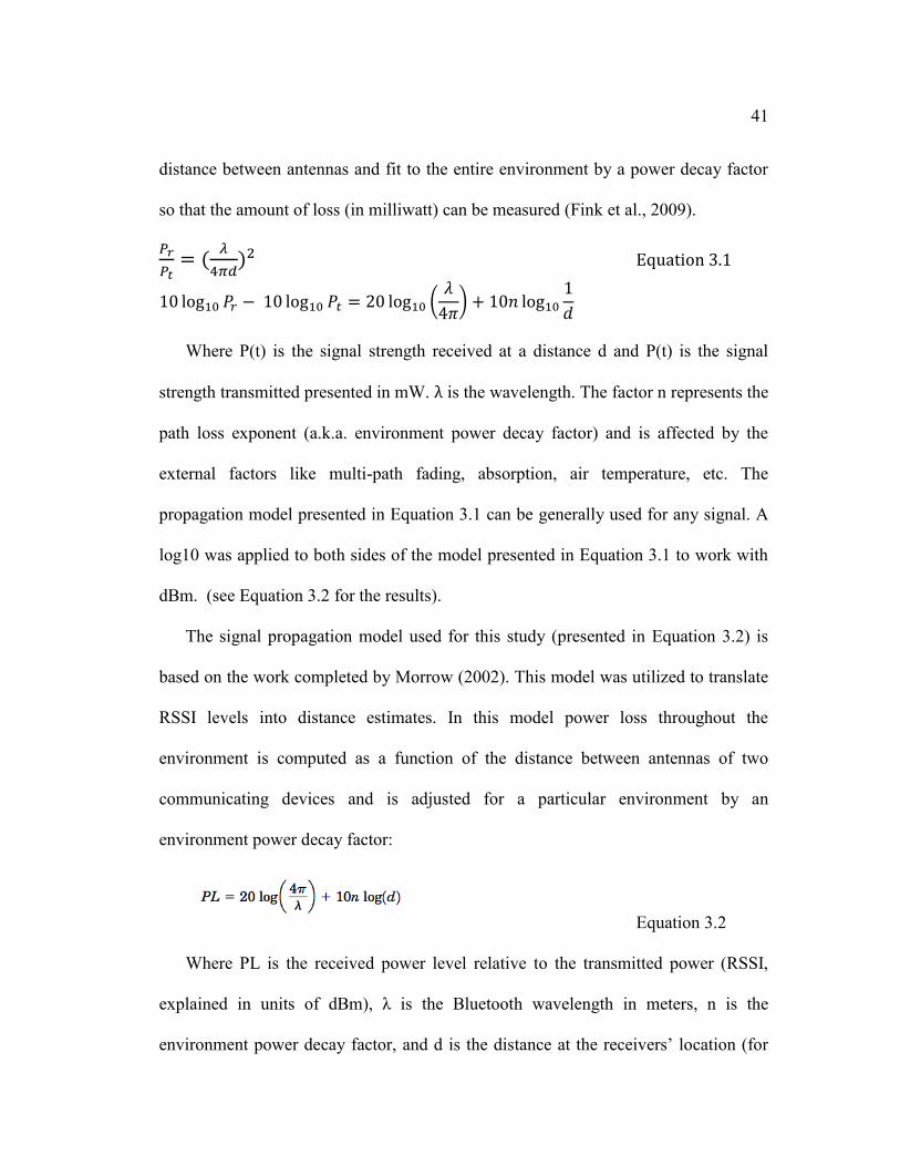
distance between antennas and fit to the entire environment by a power decay factor
so that the amount of loss (in milliwatt) can be measured (Fink et al 2009)
= ( ఒ )ଶ Equation 31 ସగௗ
10 logଵ 119875 minus 10 logଵ 119875௧ = 20 logଵ ൬ 120582 4120587൰ + 10119899 logଵ
1 119889
Where P(t) is the signal strength received at a distance d and P(t) is the signal
strength transmitted presented in mW λ is the wavelength The factor n represents the
path loss exponent (aka environment power decay factor) and is affected by the
external factors like multi-path fading absorption air temperature etc The
propagation model presented in Equation 31 can be generally used for any signal A
log10 was applied to both sides of the model presented in Equation 31 to work with
dBm (see Equation 32 for the results)
The signal propagation model used for this study (presented in Equation 32) is
based on the work completed by Morrow (2002) This model was utilized to translate
RSSI levels into distance estimates In this model power loss throughout the
environment is computed as a function of the distance between antennas of two
communicating devices and is adjusted for a particular environment by an
environment power decay factor
Equation 32
Where PL is the received power level relative to the transmitted power (RSSI
explained in units of dBm) λ is the Bluetooth wavelength in meters n is the
environment power decay factor and d is the distance at the receiversrsquo location (for
42
Bluetooth λ = 0122 meters is used) Numerous environmental factors can be
introduced into a signal propagation model such as Doppler effect multi-path fading
etc These factors can quickly increase the complexity of the model and hence reduce
its usability By considering λ = 0122 and solving equation 32 for d the signal
propagation model can be formatted as Equation 33
షరబమఱళ
d = 10 భబ Equation 33
In addition to the theoretical model presented in Equation 33 several other
empirical models were tested Empirical models were examined to check if other
nonlinear models offered a better fit than the signal propagation model An example
of one empirical model is presented in Equation 34
d = A times PL Equation 34
Where A and B are parameters of the empirical model
The parameters for different signal propagation models were fit to data generated
by obtaining signal strength readings from Bluetooth devices placed at known
distances to multiple DCUs Details of this data acquisition are presented in section
325 The Parani UD-100 Bluetooth modules utilized to generate this data report
RSSI levels in units of dBm Since the power level transmitted by most of
commercial Bluetooth-enabled devices (such as cellphones headsets PDAs etc) is
about 0 dBm (1 milliwatt) the RSSI level received at the scanner device can be used
as PL By knowing the received RSSI level and having a proper environment power
decay factor one can use the propagation model presented in Equation 33 to
calculate the distance estimate
43
The value for the power decay factor was determined empirically from generated
data A meta-heuristic optimization algorithm called particle swarm optimization was
utilized to compute the value of this parameter This method was applied to data
generated by placing Bluetooth devices at random positions with known distances to
fixed DCU locations and recording the RSSI levels received from the Bluetooth
devices (18 samples for each of the two test cell phone) The particle swarm
optimization in this study tries to find the best value for the environment power decay
factor (n) so that when the sample pairs of distance-RSSI are inserted into the
propagation model the total squared distance error is minimized An overview of
meta-heuristic algorithms and specifically the particle swarm optimization method is
presented next
323 PARTICLE SWARM OPTIMIZATION
Particle swarm optimization is a general class of metaheurstic algorithms A
metaheuristic refers to a computational method that attempts to optimize a problem
iteratively by following a general search strategy Metaheuristic algorithms are
heuristics in that in most cases optimality is not guaranteed but they have been
successfully applied to many real combinatorial and non-linear optimization
problems Metaheuristics algorithms can often generate very good solutions to
difficult optimization problems in a reasonable amount of time
Particle swarm optimization (PSO) was first introduced by Kennedy and Eberhart
and was first intended for simulating social behavior (Kennedy amp Eberhart 1995)
44
Kennedy and Eberhartrsquos work was originally influenced by earlier research completed
by Heppner and Grenander about bird flocks searching for corn (Heppner amp
Grenander 1990)
In PSO a number of entities which are referred to as particles are initialized in
the solution space of a problem or function Each particle will give an objective
function value (Poli et al 2007) In each iteration every particle moves through the
search space by combining some aspect of the history of its own current and best
locations with that of other particles with some random perturbations The next
iteration takes place after all particles have been moved Eventually the swarm (all of
the particles) as a whole like a flock of birds collectively foraging for food is likely
to move close to an optimal value A wide variety of PSO algorithms have been
proposed and the specific PSO algorithm implemented is presented next
The particle swarm optimization starts with a random value for the environment
power decay factor and then begins an iterative process to improve this value For this
study the algorithm initialized 100 random values for the environment power decay
factor (n) Each of these values which can be a candidate solution for n is called a
particle It is important to mention that the algorithm has no knowledge of the
underlying propagation model which helps to build the objective function for this
study Thus it has no way of knowing if any of the candidate solutions are near to or
far away from a near-optimum solution The algorithm simply uses the objective
function to evaluate its candidate solutions and operates upon the resultant fitness
values that is the difference between the estimated distance using an RSSI sample and
45
a random value for n in the propagation model and the actual distance for the
corresponding RSSI The algorithm maintains the sum of squares for all distance
errors and tries to minimize this value by improving the particlersquos locations The
algorithm keeps track of the best value for each particle (local optimum) and for the
entire particles population (global optimum) to move toward the best fitness value
The steps of a basic particle swarm optimization algorithm that were followed to
estimate the environment power decay factor n in the propagation model
1 Start with an initial set of particles typically randomly distributed
throughout the design space In this study particles are random values for the
environment power decay factor n in the signal propagation model For this
study a number of 100 particles were initialized with random starting values
The uniform random number generation method in visual basic was utilized to
initialize the particles
2 Calculate a velocity vector for each particle in the swarm The velocity and
position update step (step 3) are responsible for the optimization ability of the
algorithm The velocity of each particle is updated using the following
equation
119907(119905 + 1) = 119908119907(119905) + 119888ଵ119903ଵ[119909ො(119905) minus 119909(119905)] + 119888ଶ119903ଶ[119892(119905) minus 119909(119905)]
i is the index of the particle 119907(119905) is the velocity of particle i at time t 119909(119905)
is the position of the particle i at time t The parameters w 119888ଵ and 119888ଶ are user-
supplied coefficients ( 0 ≦ 119908 lt 12 0 ≦ 119888ଵ ≦ 2 0 ≦ 119888ଶ ≦ 2 ) 119909ො(119905) is the
46
individual best candidate solution for particle i at time t and g(t) is the
swarmrsquos global best candidate solution at time t These parameters were also
initialized randomly For each set of candidate solutions (aka particles)
fitness evaluation is conducted by supplying the candidate solution to the
signal propagation model Pairs of collected Distance-RSSI data are provided
to the algorithm for the fitness evaluation process For each iteration the
estimated distance is compared to the actual distance to compute the fitness
value
3 Update the position of each particle using its previous position and the
updated velocity vector to reduce the total fitness values Once the velocity for
each particle is calculated each particlersquos position is updated by applying the
new velocity to the particlersquos previous position
119909(119905 + 1) = 119909(119905) + 119907(119905 + 1)
4 Go to Step 2 and repeat until total fitness values converge to zero
The algorithm presented in this section was implemented using Microsoft Visual
Basic The algorithm was replicated a few times with particle swarm sizes of 100 and
1000 Each replication of the algorithm requires several minutes to complete and R^2
values of higher than 090 were achieved
324 SIGNAL LOCALIZATION APPROACHES
Triangulating an objects position is a method of determining the location of the
object based on its distance relative to other known locations or signal sources In
47
general there are two triangulation approaches In the first approach that is usually
referred to as triangulation knowing the coordinates (xy) of the three stations and the
distances (r) from the stations to the location of the object it is easy to find the circle
equations that represent all potential points for the location of the object relative to
those three reference points To find a single point that represents the actual location
of the object one needs to solve the three simultaneous circle equations (see Figure
31) However it is very difficult to solve these equations since they are nonlinear
Therefore there is a need for a simpler method If one pair of equations for the circles
are taken and subtracted one from the other the result will be the equation of the line
passing through the two points of intersection of the two circles (see Equation 35)
ଶ
ቊCircle a (x minus xୟ)ଶ + (y minus yୟ)ଶ = rୟ Equation 35 Circle b (x minus xୠ)ଶ + (y minus yୠ)ଶ = rୠଶ
ଶCircle b minus Circle a 2x(xୟ minus xୠ) minus ൫xୟଶ minus xୠଶ൯ + 2y(yୟ minus yୠ) minus ൫yୟଶ minus yୠଶ൯ = rୠଶ minus rୟ
The big advantage being that the result is therefore a linear equation which is
much easier to deal with Next by subtracting any other two of the three circle
equations a second line equation would be obtained The intersection of these two
lines is the location of the object Both line equations will pass through two points of
intersection between each pair of circles and one of these intersection points is the
point that the object is located at
48
Figure 31 Intersection of Three Circles at a Single Point
The triangulation method explained so far is very simple and works as long as
these three circles really intersect at a single point However that is not always the
case In signal propagation the distance estimates always have some error which
prevents the three circles from intersecting at a single point Thus there would be a
need for a different algorithm to handle such errors and still be able to estimate the
location of the object To mitigate the errors resulting from the propagation model a
trilateration process can be utilized In geometry trilateration is an iterative process to
determine absolute or relative location of an unknown point by measurement of
distances from a number of known points using the geometry of circles andor
spheres Trilateration is extensively used in commercial navigation applications
including Global Positioning Systems (GPS)
49
In the case of a two-dimensional problem when it is known that a point is located
on at least three curves such as the boundaries of three circles then the circle centers
and the three radii provide sufficient information to narrow the possible locations
down to one location However if these three circles do not intersect on a single point
an iterative process can be used to relatively scale the circles radii to force these three
circles to intersect at one point This extra step is needed when errors resulting from
the inaccuracy of the propagation model are present Both algorithms explained in
this section are implemented using Python language and are presented in the
Appendix section B
325 TRILATERATION STUDY TO DEVELP A SIGNAL PROPAGATION
MODEL
For this experiment three Bluetooth scanner devices were used Bluetooth scanners
were attached to 24 GHz omnidirectional antennas to match the setup configuration
implemented for a research project conducted for Oregon Department of
Transportation A large parking lot on Oregon State University campus was selected
to conduct this experiment Figure 32 illustrates the test site for this experiment The
antennas were placed in an lsquoLrsquo shape configuration 10 meters separated from each
other (see Figure 33 for setup arrangement)
50
Figure 32 Trilateration Test Experiment Setup
Figure 33 Scanners Arrangement in an L Shape
51
For this experiment a stratified random sampling approach was selected to evenly
distribute sample locations across the discovery range of the units The discovery
range (which represents an imaginary intersection with its four approaches) was
divided into 9 different areas Defined areas (numbered from 1 to 9 in Figure 33)
were sorted in a random order and for each area two random samples were collected
Pairs of locations (x y) were generated randomly for each defined area To facilitate
the test process Table 32 was developed For each row in this table two
experimental Bluetooth-enabled cell phone devices were placed at the location noted
on column three Next signal strength levels from all three Bluetooth scanners were
measured and recorded (ie RSSI 1 RSSI 2 and RSSI 3) The signal propagation
model was calibrated based on the collected data
Table 32 Random locations selected for Test Cell Phone 1
Region Location ( x y ) RSSI 1 RSSI 2 RSSI 3
1 7 -4 22 -79 -86 -58
2 1 1 2 -52 -70 -66
3 8 11 21 -69 -69 -68
4 5 10 6 -61 -59 -70
5 4 2 11 -57 -73 -62
6 5 13 12 -68 -61 -71
7 7 -2 16 -72 -71 -62
8 1 -1 1 -60 -74 -63
52
9 9 19 23 -70 -59 -73
10 3 22 2 -81 -57 -86
11 8 7 23 -69 -73 -65
12 2 12 0 -60 -52 -72
13 4 3 9 -55 -73 -61
14 6 16 10 -64 -59 -70
15 6 24 13 -80 -62 -73
16 2 11 2 -63 -58 -78
17 3 18 0 -65 -44 -68
18 9 19 18 -77 -67 -72
326 FITTING THE ENVIRONMENT POWER DECAY FACTOR
Using the data collected during the study presented in section 325 and by utilizing a
particle swarm optimization a number of mathematical models were developed to
describe the signal propagation phenomena (See Table 32 for the data) As it was
explained earlier these models include the theoretical signal propagation model based
on Morrowrsquos work (2002) and a few empirical models For each mode an R-square
value was calculated based on the data used to fit modelrsquos parameters Higher R-
square values indicate that the model (and its parameters) do a better job in
converting RSSIs into distance estimations Among these models however the model
based on the theoretical power loss model generated the highest level of accuracy
53
Estimated Distance Error
0 20 40 60 80
The propagation model equation with its calibrated parameters is presented in
Equation 36 that has a value of 168 for n
RSSI = 168 logଵ(d) + 346 Equation 36
As a part of the model development process the distance estimates for each
sample location based on the recorded RSSI levels were compared to the actual
distance from the sample location to the DCUs Figure 34 illustrates actual and
estimated distances versus recorded RSSIs In the figure actual distance samples for
each random location is marked using dots for each test cell phone
50
0
-50
Error
(dis
tance) -100
-150
-200
-250-
-300-
Estimated Distance
Error
RSSI-
Figure 34 Error Comparisons for Estimated Distances Using the Developed Signal
Propagation Model for Both Test Cellphones
100
54
327 ACCURACY ASSESSMENT
Next a second field test was conducted to evaluate the accuracy of the developed
signal propagation model This experiment was completed at the same test site with
similar setup configuration An assessment of the propagation model (Equation 36)
accuracy was conducted using a number of location-RSSI pairs The propagation
model developed in previous step was used to estimate the location of the Bluetooth
device merely based on the RSSI levels recorded on three DCUs In this step the
RSSI values recorded from three DCUs were translated into three distance estimates
Finally the iterative trilateration algorithm was utilized to obtain relative location
estimates for each sample reading The location estimations were compared against
actual locations and the distance between these two points were used as the error
value The results are summarized in Table 33 The first two columns show the
location of the test cell phone relative to the antenna 1 (see Figure 33) The next three
columns show the distance estimates from each antenna using the recorded RSSI
Columns six and seven show the estimated location using the iterative trilateration
technique The last column represents the Euclidean distance between the actual
location and the estimated location that serves as the error
55
Table 33 Signal Propagation Model Accuracy Test Results
Actual Location (xy) Estimated Distances (m) Predicted Location Linear
Distance -4 22 235479 266011 128617 69664 169191 12086 1 2 105718 166782 166782 63365 633656 6876 11 21 227846 250745 113351 76476 178288 4614 10 6 98085 128617 13625 80814 753122 2454 2 11 174415 189681 90452 85775 157753 8128 13 12 174415 174415 128617 99999 132830 3262 -2 16 281277 296543 159149 83619 188778 10754 -1 1 159149 197314 143883 71398 109409 12848 19 23 204947 159149 182048 13624 119434 12293 22 2 189681 143883 182048 13391 106354 12193 7 23 250745 281277 143883 69750 169301 6069 12 0 113351 5992 220213 12670 036762 0765 3 9 143883 189681 113351 63983 118166 4413 16 10 182048 159149 120984 12067 149317 6307 24 13 235479 113351 189681 23794 16048 3054 11 2 113351 75186 151516 12333 693284 5109 18 0 159149 44654 21258 16590 468432 4891 19 18 243112 220213 159149 12275 170651 6788
Ave 6828 STD 3763
328 CONCLUSIONS AND LIMITATIONS
Although the estimated locations obtained through the trilateration method are close
to actual locations on average the test results are not satisfactory on an individual
case basis In those cases with large errors the predicted locations are a few meters
off from the actual location of the test cell phones
There are several sources of inaccuracy in the environment that makes the
trilateration approach inappropriate for the outdoor application proposed in this
research The signal strength indicator itself is a measure that has some noise in its
56
nature Moreover physical phenomena such as the Doppler effect multi-path and
fading are other factors that can introduce error to the signal strength Additionally
the dynamic movement of physical objects on the road (ie vehicles bicyclists and
pedestrians) is another factor that makes the outdoor trilateration based on the signal
strength challenging
In the rest of this research another approach based on the wireless received signal
strength is pursued The new approach is less sensitive to the natural noise and
fluctuation within the RSSI levels Furthermore the new approach utilizes RSSI data
from a group of detections for the same device to obtain location data and does not
compare detections from different devices
33 VEHICLE POINT DETECTION SYSTEM
In this section a different approach for collecting vehicle movement data is presented
The objective is to explore and test how the DCUs that collect data wirelessly can be
utilized as point detection units A point detection unit identifies the time that a
vehicle has just passed an imaginary line on the road that originates from the data
collection unit By utilizing multiple DCUs that function as point detection units a
vehicles trajectory through a road segment can be approximated The objective of this
method is less ambitious with respect to the vehicle movement data level of detail
sought in the Trilateration approach To achieve this goal time stamped wireless data
obtained by a DCU from passing vehicles which includes RSSI levels is utilized to
estimate when a vehicle was the closest to the data collection unit When multiple
57
DCUs are utilized on a road segment this information can be used to derive several
performance measures such as travel times and intersection delay
The remainder of this section starts with a presentation of the background theory
supporting how RSSI data can be used to estimate when vehicles just pass a DCU
This theory is implemented in a RSSI-based point detection algorithm that is
described next Finally a validation test experiment and results for the proposed
algorithm are presented
331 VEHICULAR MOVEMENTS NEAR A DATA COLLECTION UNIT
AND THE RSSI-DISTANCE RELATIONSHIP
Vehicle trajectories as a vehicle travels by a DCU can take many different forms
Vehicles may pass the DCU at a fairly constant speed or could be accelerating or
decelerating Vehicles may also stop near the DCU before passing it If a vehicle
contains a detectable wireless device the DCU will be detecting the vehicle multiple
times as it travels in the coverage area of the DCU In this section theoretical signal
propagation models are utilized to understand how the signal strength of the DCU
detections will vary over time for different vehicle trajectories
In this research it is assumed that a DCU is located at the stop line located on a
signalized intersection The vehicle trajectories analyzed include through passes and
stops due to a red light The stops may occur relatively close or far from the stop line
For these three cases numerical examples of RSSI levels as a function of distance
and time (ie vehicle trajectory) are generated and plotted (see Figures 35 36 and
58
37) The predicted RSSI levels as a function of distance and time are obtained from
the model presented in section 325 (Equation 36) The plots show the time on the X
axis (in seconds) as the vehicle enters and leaves the intersection the predicted RSSI
level on the left Y axis (in dbm) and the distance from the perpendicular line on the
road extended from the DCU on the right Y axis (in meters) It is assumed that the
design vehicle has a constant speed of 35 MPH when approaching the stop line and it
takes about 10 seconds to stop or return to the constant speed if a stop occurs For
example assume that a vehicle at time t is 90 meters away from the perpendicular
line extended on the road from the DCU Assuming that the lateral distance from the
vehiclersquos lane to the DCU is about 8 meters (26 feet is the width of two standard
lanes) this will result in a direct distance of radic8ଶ + 90ଶ = 9035 meters from the
DCU Using the propagation model introduced in Equation 36 the expected RSSI
level at this distance is -67dbm The output of the propagation model in Equation 36
is a positive number since the propagation model represents the RSSI level change as
the signal travels over a given length (path loss) An average cell phone transmits a
power level of 1 milliwatt (0 dbm) Therefore the RSSI level at a distance of 9053
meters should be -67 dbm
To consider the impact of environmental noise on the RSSI levels recorded and
the vehiclersquos movement effect on the RSSI levels a random value from a normal
distribution was also added to RSSI values predicted by equation 36 These plots
(Figures 35 36 and 37) show a sample of RSSI behavior as a vehicle enters and
leaves a signalized intersection
59
0
200
400
600
800
1000
-120
-100
-80
-60
-40
-20
0 0 5 10 15 20 25 30 35
RSSI
Distance
Figure 35 Highlighted Example of a Through Pass RSSI and Distance Sample Data
0
100
200
300
400
500
600
700
800
-100 -90 -80 -70 -60 -50 -40 -30 -20 -10
0 0 5 10 15 20 25 30 35
RSSI
Distance
Figure 36 Highlighted Example of a Stop Far From Stop Line RSSI and Distance
Sample Data
60
-100 0 100 200 300 400 500 600 700 800
-100
-80
-60
-40
-20
0 0 5 10 15 20 25 30 35
RSSI
Distance
Figure 37 Highlighted Example of a Stop Near Stop Line RSSI and Distance Sample
Data
Figure 35 shows the scenario when a vehicle arrives at the intersection during a
green light In this example there is no congestion at the intersection Therefore the
vehicle travels through the intersection with a constant speed As the vehicle enters
the discovery range of the DCU located at the intersection the RSSI levels start to
increase until a maximum point and then decrease until the vehicle leaves the
intersection Theoretically the maximum point is recorded when the vehicle was the
closest to the DCU Therefore the time-stamped data record with the highest RSSI
value is the best estimate of the time that vehicle has passed the DCU
Figure 36 illustrates the second scenario in which the vehicle stops due to the red
light In this case the vehicle stops far from the stop line because a queue has formed
in front of the stop line During the time that vehicle has stopped it is unlikely to see
large differences in RSSI levels since the vehiclersquos distance to the DCU remains
constant Once the vehicle starts to move again the RSSI level increases as the
61
vehicle gets closer to the stop line and then decreases as the vehicle continues beyond
the stop line Again the time-stamped data record with the maximum RSSI level best
estimates the time the vehicle passed the stop line
Figure 37 shows the third scenario in which the vehicle also stops due to the red
light In this scenario however the vehicle stops very close to the stop line In this
case it is not easy to use the RSSI data to predict when vehicle has passed the stop
line since it is less likely that the time-stamped data record with the maximum RSSI
value is the best estimate of the time that vehicle has passed the stop line This can be
attributed to the effect of noise on the RSSI levels which are often greater than the
predicted difference in RSSI levels when a vehicle stops close to the DCU and when
it is adjacent to the DCU This complexity is usually magnified in real-world
scenarios in which the noise levels of the RSSI data can be significantly higher due to
other factors such as interference and the presence of other vehicles
332 POINT DETECTION ALGORITHM
In this section a point detection algorithm using time-stamped RSSI data associated
with a traveling vehicle is presented The algorithm presented here utilizes the
distance-RSSI relationship introduced in section 331 and generates an estimate for
the time that a vehicle has just passed an imaginary line on the road that originates
from the data collection unit A sample of data collected from one DCU is shown in
Table 34 These data represent a sample of MAC addresses collected over a seven-
minute period from one of the installed DCUs Truncated MAC addresses are shown
62
in the first column and the timestamps are shown in the second column For the
purposes of this research the combination of a truncated MAC address and its
corresponding timestamp (ie date and time) are referred to as detection The three
columns on the left in Table 34 show the MAC addresses in the sequence that they
were detected by the DCU The three columns on the right in Table 1 show the same
data sorted by MAC address Nine different MAC addresses were detected over the
seven-minute period A single MAC address may be detected multiple times as it
passes the detection zone of a DCU The antenna attached to the DCU utilized to
collect the sample data in Table 34 covers a large area of the road (approximately
1200 feet of the road 600 feet before and after the DCU) Since a vehicle traveling
on this road at a particular speed will be in the length of road covered by the DCUs
antenna for couple of seconds multiple detections of MAC addresses should occur
(see Figure 38) For the sample data presented in Table 34 the speed limit was 45
MPH which requires an average vehicle 18 seconds to travel the length of the
antennarsquos discovery range The combined effects of the probabilistic nature of the
Bluetooth inquiry procedure the variations in radio frequency signal strength of the
radios of Bluetooth enabled devices and unknown and uncontrollable factors
affecting radio frequency communications (eg interference multi-path) explain why
active Bluetooth devices in different passing vehicles moving at the same speed may
be detected a different number of times
To facilitate the description of issues related to locating vehicles location based
on MAC address data the concept of a group of MAC addresses will be defined and
63
illustrated A group will be defined as a collection of MAC address detections for the
same MAC address that represent one trip (in a single direction) of the corresponding
Bluetooth-enabled device through the length of road covered by the DCUs antenna
along the road that it is monitoring For example the trip illustrated in Figure 38
shows a group size of 3
Figure 38 Multiple detections within the DCUs detection zone
64
Table 34 Sample of MAC Address Data from an Installed Bluetooth DCU
MAC Addresses in Sequence MAC Add Date Time 283AC3 6262012 170009 0D1BA6 6262012 170013 0D1BA6 6262012 170021 5F9FB8 6262012 170053 5F9FB8 6262012 170057 A5E228 6262012 170057 5F9FB8 6262012 170102 5F9FB8 6262012 170106 5F9FB8 6262012 170110 5F9FB8 6262012 170114 5F9FB8 6262012 170119 ACC9B5 6262012 170127 ACC9B5 6262012 170131 ACC9B5 6262012 170147 ACC9B5 6262012 170151 A5E228 6262012 170159 A5E228 6262012 170215 C2BBD0 6262012 170306 9C09B2 6262012 170310 C2BBD0 6262012 170310 9C09B2 6262012 170315 C2BBD0 6262012 170315 C21146 6262012 170433 C21146 6262012 170437 C21146 6262012 170441 86F2DF 6262012 170532 A5E228 6262012 170608 A5E228 6262012 170702
MAC Addresses Sorted MAC Add Date Time 0D1BA6 6262012 170013 0D1BA6 6262012 170021 283AC3 6262012 170009 5F9FB8 6262012 170053 5F9FB8 6262012 170057 5F9FB8 6262012 170102 5F9FB8 6262012 170106 5F9FB8 6262012 170110 5F9FB8 6262012 170114 5F9FB8 6262012 170119 86F2DF 6262012 170532 9C09B2 6262012 170310 9C09B2 6262012 170315 A5E228 6262012 170057 A5E228 6262012 170159 A5E228 6262012 170215 A5E228 6262012 170608 A5E228 6262012 170702 ACC9B5 6262012 170127 ACC9B5 6262012 170131 ACC9B5 6262012 170147 ACC9B5 6262012 170151 C21146 6262012 170433 C21146 6262012 170437 C21146 6262012 170441
C2BBD0 6262012 170306 C2BBD0 6262012 170310 C2BBD0 6262012 170315
In the data shown in Table 34 the smallest time interval observed between
detections with the same MAC address is four seconds because the DCUs were
programmed to repeat the initiation of an inquiry procedure that is four seconds in
length to cover the entire Bluetooth frequency spectrum and hence detect all
Bluetooth-enabled devices nearby Table 34 also shows different MAC addresses
65
that have the same timestamps (eg 9C09B2 and C2BBD0) These MAC
addresses were detected in the same inquiry period and represent either multiple
devices in the same vehicle or multiple vehicles with active devices passing the
reader at about the same time
For the purpose of identifying those MAC address detections that correspond to
when the vehicle was the closest to the imaginary line originating at a DCU Figure
39 shows an example in which a vehicle was detected three times passing a DCU
(shown as location numbers 1 2 and 3) In this example at the timestamp of the
MAC address detected at location number 2 the vehicle was closest to the DCU For
vehicles that arrive at an intersection and have to wait for the traffic signal to change
their number of MAC address detections (or group size) can grow rapidly This can
result in large errors when calculating traffic performance measures such as travel
time samples when an inappropriate timestamp is chosen
Figure 39 Schematic representation of multiple detections in a single trip forming a
group
66
As explained before the method developed in this research to select a single
MAC address detection is based on the RSSI The RSSI is known to be correlated
with distance where a larger RSSI value indicates that the DCU and Bluetooth device
are closer together than a lower RSSI value (Awad et al 2007 Kotanen et al 2003
Pei et al 2010)
Although RSSI is correlated with distance it is also affected by the movement of
the Bluetooth mobile device In theory moving toward and away from the DCU can
generate Doppler effect which in some cases can reduce the signal strength level
received at the DCU Multi-path is another propagation phenomenon that results
when radio signals reaching the receiving antenna come from two or more paths This
phenomenon can have both constructive and destructive effects on the signal strength
Modeling the effect of these phenomena is complex and beyond the scope of this
research however it is accounted for indirectly by adding the noise adjustment to the
data in Figures 35 36 and 37 For example in Figure 39 a device that is stationary
at location 2 will often generate a MAC address detection with a higher RSSI than
when the device is at location x but in movement For DCUs located at signalized
intersections this implies that using the MAC address detection with the highest
RSSI is often not the detection that represents the time the vehicle was closest to the
DCU
For a DCU located at a signalized intersection the method used to identify the
MAC address detection representing the time when the vehicle is closest to the DCU
is based on the rate of change in RSSI values between consecutive MAC address
67
detections within a group In this approach the MAC address detection selected is
that detection after which the subsequent RSSI values decrease at the highest rate
This rate of change can be obtained using following equation 37
େ୳୬୲ ୗୗ୴୧୭୳ୱ ୗୗ Equation 37 େ୳୬୲ ୧୫ୱ୲ୟ୫୮୴୧୭୳ୱ ୧୫ୱ୲ୟ୫୮
In those cases where this decreasing rate of change is not observed the last MAC
address detection in a group is saved Often the MAC address detection selected also
has the largest RSSI value Intuitively the method described attempts to detect the
time that a vehicle has just started to leave the intersection after passing the DCU
Figure 310 shows a real example of RSSI data over time for multiple reads of the
same Bluetooth-enabled devices during a single probe vehicle trip past a DCU In this
example a probe vehicle carrying two Bluetooth-enabled cell phone devices
approached an operating DCU at the signalized intersection of SW Durham Rd and
Highway 99W The probe vehicle stopped for a while at this intersection and then left
the discovery area of the DCU The dashed line represents the manually recorded
time that corresponds to when the probe vehicle just passed the imaginary line
perpendicular to the road extending from the DCU In Figure 310 the most accurate
timestamps are identified by the larger squares for both cell phones These
timestamps represent the time the probe vehicle started to leave the intersection and
are characterized by a rapid decrease in the RSSI levels after these points
68
Figure 310 RSSI values over time for two devices in a probe vehicle arriving and
waiting at an intersection
333 VALIDATION EXPERIMENTS
A series of experiments were conducted to test the accuracy of the proposed point
detection system in three different environments The purpose of these experiments
was to assess differences between the time stamp of the automatically selected record
(utilizing the point detection algorithm presented in section 332) and the time the
vehicle crosses an imaginary line extending from the DCU antenna across and
perpendicular to the road A schematic of the general physical experimental setup is
presented in Figure 39 A DCU and antenna are installed at some location adjacent to
the roadway being monitored (point A in Figure 39) The distance d from point A in
69
Figure 39 and the roadway will vary depending on the available mounting structures
at the location where the DCU is placed
In these experiments a probe vehicle containing active Bluetooth devices with
known MAC addresses travels past a DCU multiple times At the same time there is a
person operating a laptop computer that is communicating with the DCU The
communication of the DCU and laptop computer permits synchronization of the DCU
time and laptop time Software is provided to help the laptop operator record the
exact time that a vehicle passes the DCU (crosses line AB in Figure 39) When the
front of the vehicle just passes line AB in Figure 39 the operator will press the
ldquoEnterrdquo key on the laptop keyboard When this key is pressed a time stamp will be
automatically generated and stored in a file
If feasible in a particular test environment the vehicle will be driven past the DCU
at a fixed speed Different speeds can be examined to see if speed has an effect on the
differences between the timestamp of the selected record and the time the vehicle
passes the DCU
The DCU will be scanning continuously during the experiment Knowing the time
that the vehicle passed the DCU and assuming a constant travel speed the time that
the vehicle was a specific distance from the DCU can be computed For example the
time that the vehicle is at points 1 2 and 3 in Figure 39 can be computed from the
time the vehicle passed the DCU (point x) The distance that each point is from point
x (d1 d2 d3) is known By matching the MAC address timestamps to various
locations it is possible to map RSSI values to different vehicle locations
70
The first test environment used for validation was a low traffic free flowing rural
road near Corvallis Oregon (Camp Adair Road adjacent to EE Wilson Wildlife Area
ndash Figure 311) Due to low traffic volumes it was possible to drive at various constant
speeds past the DCU The probe vehicle traveled passed the DCU 30 times (15 times
traveling east and 15 times traveling west) for each speed tested The speeds tested
were 25 35 and 45 mph The DCU was located 36 feet from the road and the antenna
was mounted on a tripod at a height of 70 inches Two different cell phones with
Bluetooth communications active were used in the tests The responses computed
from the recorded data were the time differences between the MAC address records
with the highest RSSI reading and the times the vehicle crossed the line drawn from
the DCU perpendicular to the road A histogram of all the test results is shown in
Figure 312 Most time differences are less than two seconds with a maximum
difference of 75 seconds The average time difference was 023 seconds with a
standard deviation of 137 seconds Negative time differences occur when the time
stamp of the highest RSSI record occurs after the vehicle passes the DCU
71
Figure 311 DCU installation on Camp Adair Road Benton County
Figure 312 Histogram of the difference between the time the probe vehicle passed
the DCU on Camp Adair Road and the MAC address record with the highest RSSI
72
The second test environment was Wallace Road which is located on the west side
of the city of Salem Oregon This road is also a free-flowing road with no signals
located near the DCU but a single signal between the DCU locations The Oregon
Department of Transportation (ODOT) Intelligent Transportation Systems (ITS) Unit
operates a test site on this road located at latitude-longitude of N 44972858 and W -
123066321 (see Figure 313) Wallace Road runs north and south with two lanes in
both directions and the speed limit is 45 MPH Forty total probe vehicle runs (20
traveling northbound and 20 traveling southbound) were made past the DCU with
two different cell phones with active Bluetooth communications present in the
vehicle
The responses computed from the recorded data were the time differences
between the MAC address records with the highest RSSI reading and the times the
vehicle crossed the line drawn from the DCU perpendicular to the road A histogram
of all the test results is shown in Figure 314 Most time differences are less than two
seconds with a maximum difference of five seconds The average time difference
was 023 seconds (the same as for Camp Adair Road) with a standard deviation of
124 seconds Negative time differences occur when the time stamp of the highest
RSSI record occurs after the vehicle passes the DCU
73
Figure 313 DCU Location on Wallace Road Salem Oregon
Figure 314 Histogram of the difference between the time the probe vehicle passed
the DCU on Wallace Road and the MAC address record with the highest RSSI
74
The third test environment was along Highway 99W in Tigard Oregon Five
DCUs have been installed at five different intersections (see Figures 315 and 316)
Figure 315 Southernmost DCU locations on Highway 99W Tigard Oregon
75
Figure 316 Southernmost DCU locations on Highway 99W Tigard Oregon
The Highway 99W tests were conducted at DCU 12 which is located at a
signalized intersection Forty total probe vehicle runs (20 traveling northbound and 20
traveling southbound) were made past the DCU with two different cell phones with
active Bluetooth communications present in the vehicle Two responses were
recorded and analyzed
The first response computed from the recorded data were the time differences
between the MAC address records with the highest RSSI reading and the times the
vehicle crossed the line drawn from the DCU perpendicular to the road This is the
same response as used in the prior test environments which were both free-flowing
76
roads A histogram of all the test results is shown in Figure 317 Most time
differences are less than two seconds with a maximum difference of 43 seconds The
average time difference was 31 seconds with a standard deviation of 99 seconds
The results were similar to the other test environments except for five test runs where
the response was greater than 11 seconds (42 41 18 12 and 12 seconds) With these
five responses removed the average maximum and standard deviation of the
response are -003 seconds 33 seconds and 13 seconds respectively
In those instances where large time differences were observed the probe vehicle
was stopped by the signal and stationary The stationary position of the probe vehicle
was one or two vehicle lengths before the line drawn from DCU 12 perpendicular to
the road When stationary yet close to the DCU higher RSSI readings were obtained
than when the probe vehicle was moving across the line drawn from the DCU In this
case the MAC address record with the highest RSSI reading occurred when the probe
vehicle was close in distance to the line drawn from the DCU but still relatively far
with respect to time since the vehicle was waiting for a green light to proceed As
seen in Figure 312 all of the relatively large time differences are positive
differences which occur when the MAC address with the highest RSSI reading
occurs before the probe vehicle passes the line drawn from the DCU Negative time
differences occur when the time stamp of the highest RSSI record occurs after the
vehicle passes the DCU In such cases as just described the accuracy of the travel
time samples generated will be reduced The time interval between when the highest
RSSI reading was recorded and when the vehicle passed the DCU will be added to
77
the travel time along the road section that occurs after the signal Similarly this time
difference will not be included in the travel time for the road section occurring before
the signal
Figure 317 Histogram of the difference between the time the probe vehicle passed
DCU 12 on Highway 99W and the MAC address record with the highest RSSI
The second response recorded and analyzed is based on a method to eliminate
these occasional large errors caused when a vehicle stops just before passing the
DCU In this method the single record selected from a group of MAC addresses is the
record after which the subsequent RSSI values decrease at the highest rate In those
78
cases where this decrease is not observed the last record in a group is saved Since the
highest RSSI record can often be when a vehicle stops close to but before passing the
DCU the RSSI values should also decrease rapidly once a vehicle passes the DCU
after the vehicle has a green signal
Figure 310 showed the time stamps and associated RSSI for two Bluetooth
devices (two cell phones) when a vehicle stops and waits close to the DCU as it
travels through the intersection The large circles represent the time stamps associated
with the highest RSSI Since the vehicle stops near the DCU the time stamps which
are associated with the highest RSSI are considerably earlier than the time when the
vehicle passes the DCU
The responses computed using this method were compared to the times the probe
vehicle crossed the line drawn from the DCU perpendicular to the road A histogram
of all the test results is shown in Figure 318 Most time differences are less than two
seconds with a maximum difference of 21 seconds The average time difference was
22 seconds with a standard deviation of 41 seconds The performance is more
accurate and consistent than saving the record with the highest RSSI value
79
Figure 318 Histogram of accuracy of the time stamp before the RSSI values rapidly
decrease
80
4 APPLICATION CASE STUDIES
The Bluetooth-based vehicle point detection system introduced in this research can be
employed to collect vehicle movement data in different areas of the transportation
system The vehicle movement data collected can then be utilized to estimate traffic
performance measures for analysis and planning studies
In this section two particular applications of the Bluetooth-based vehicle
point detection system are presented In these applications vehicle movement data
are utilized to derive two commonly used traffic performance measures intersection
delay and travel time The most common current data collection methods employed to
collect data to estimate these performance measures are expensive and in some cases
inaccurate (Bonneson amp Abbas 2002 Middleton et al 2009 Balke et al 2005)
and labor intense In contrast the data collection method developed in this research
provides a low-cost solution to estimate these performance measures with high levels
of accuracy
41 TRAVEL TIME STUDY
The use of time-stamped media access control (MAC) address data acquired from
Bluetooth-enabled devices to collect travel time data has received significant attention
in recent years However past research has mainly focused on the application of
Bluetooth technology to obtain travel time data on free flowing roads A smaller
amount of research has addressed the use of Bluetooth-based data collection systems
81
on arterial roads and in particular for the collection of travel times between
signalized intersections where the travel time accuracy has been questionable The
point detection system presented in Chapter 3 was utilized to develop a methodology
to collect accurate travel time data between signalized intersections using a
Bluetooth-based data collection system The proposed RSSI-based travel time data
collection method can be implemented using any wireless technology that provides a
unique identification number to distinguish between different mobile devices and an
associated signal strength measurement during the wireless communication process
The results of this research have been attested with a Bluetooth-based data
collection system that consists of five DCUs permanently installed at consecutive
signalized intersections along an urban high-volume signalized arterial (ie
Highway 99W) running north-south in Tigard OR This system was introduced and
used earlier in Chapter 3 to perform a timestamp selection accuracy study These
DCUs are located at intersections because of the availability of power and access to a
communications network through signal control cabinets Figure 41 shows the five
consecutive signalized intersections (approximately one mile apart from each other)
where DCUs are installed ie Durham Rd McDonald St Johnson St 217 NB ramp
and 64th Ave
82
Figure 41 Location of Bluetooth DCUs on Highway 99W (Tigard OR)
411 GENERATION OF TRAVEL TIME SAMPLES USING MAC ADDRESS
DATA
To begin the discussion of travel time sample generation the specific road segment of
interest must be defined In this research the road segments for which travel time
samples are desired start at an imaginary line extending from a roadside DCU across
and perpendicular to the road and end at a similar line drawn from another DCU at a
different location along the same road Travel time samples are computed as the time
difference between detections of the same MAC address at each DCU This research
focuses on the case when these roadside DCUs are installed at signalized intersections
83
located on arterial roads ldquoGround truthrdquo travel times for a specific vehicle will be
defined as the time difference between when the vehicle crosses the previously
defined imaginary lines (determined and recorded by an observer inside the probe
vehicle) All travel time sample accuracy results are relative to the ground truth travel
times
412 TRAVEL TIME SAMPLE GENERATION SUPPLEMENTED WITH
RSSI DATA
Based on the definition of a road segment introduced earlier the most accurate travel
time samples generated from MAC address data will utilize those MAC address
detections that correspond to when the vehicle was the closest to the imaginary line
originating at a DCU As explained in section 332 the method developed in this
research to select a single MAC address detection from the group is based on the
RSSI The method used to identify the MAC address detection representing the time
when the vehicle is closest to the DCU is based on the rate of change in RSSI values
between consecutive MAC address detections within a group In this approach the
MAC address detection selected is that detection after which the subsequent RSSI
values decrease at the highest rate In those cases where this decreasing rate of change
is not observed the last MAC address detection in a group is saved Often the MAC
address detection selected also has the largest RSSI value Intuitively the method
84
described attempts to detect the time that a vehicle has just started to leave the
intersection after passing the DCU
An experiment was conducted on Highway 99W in Tigard Oregon to assess
differences between travel times calculated using time-stamped MAC addresses
associated with the first detection last detection and average of the first and last
detections in a group and travel times calculated with time-stamped MAC address
detections selected utilizing RSSI data presented in section 332 The experimental
data were collected from a probe vehicle containing two active Bluetooth devices
(cell phones 1 and 2) with known MAC addresses that traveled past the five DCUs
installed on Highway 99W multiple times A laptop computer was used in the
experiment to facilitate the collection of manual travel times An observer pressed the
ldquoEnterrdquo key on the laptop when the vehicle passed the DCUs to instruct a software
application to automatically generate and store a timestamp in a file The DCUs
scanned continuously during the experiment A total of 20 probe vehicle runs (10
traveling northbound and 10 traveling southbound) were made past all five DCUs
Adjacent signalized intersections on Highway 99W were paired to form a total of
four road segments with an average length of one mile For each probe vehicle run on
each defined segment four different travel time samples were generated utilizing the
various methods for selecting MAC address detections form a group Next the
calculated travel times were compared against the ground truth travel times
collected The absolute difference between the calculated travel time samples and
ground truth travel times were recorded as the error for each travel time calculation
85
method Table 41 summarizes the errors for the calculated travel time samples using
different timestamp selection approaches for cell phone 1 for the road segment
between Johnson St and the 217 NB Ramp
Table 41 Cell Phone 1 Sample Probe Vehicle Test Results for the Road Segment
between Johnson St and the 217 NB Ramp
Non RSSI-based Methods RSSI
Metho d
Ground Truth Travel Times
Absolute Error Relative to Ground Truth Travel Times
Run Firs t Last (F+L)
2 First Last (F+L)2
RSSI Method
1 128 135 131 125 124 004 011 007 001 2 225 148 206 149 149 036 001 017 000 3 212 212 212 203 203 009 009 009 000 4 249 136 212 139 135 114 001 037 004 5 151 301 226 251 253 102 008 027 002 6 238 134 206 137 133 105 001 033 004 7 141 259 220 229 229 048 030 009 000 8 258 245 251 239 240 018 005 011 001 9 158 256 227 247 246 048 010 019 001
10 341 202 252 156 154 147 008 058 002 11 151 143 147 142 140 011 003 007 002 12 142 140 141 134 134 008 006 007 000 13 246 233 239 241 240 006 007 001 001 14 202 140 151 138 136 026 004 015 002 15 203 203 203 156 153 010 010 010 003 16 234 229 231 226 225 009 004 006 001 17 144 148 146 139 138 006 010 008 001 18 246 248 247 243 242 004 006 005 001 19 155 205 200 153 154 001 011 006 001 20 258 304 301 303 303 005 001 002 000
AVG (sec) 2785 73 147 135 STDV (sec) 2988 64 1414 122
86
The test results presented in Table 41 clearly show that the travel time samples
obtained with the RSSI-based method are significantly more accurate and precise
than those obtained with any other method For this example road segment the
average travel times generated using the RSSI-based method had an average error of
135 seconds compared to the ground truth travel times recorded On the other
hand the travel times generated using first-to-first MAC address timestamps (ie the
most common approach cited in the literature to obtain travel time samples) had an
average error of 2785 seconds which is significantly higher than the calculated error
for the proposed method Table 42 summarizes the test results for all four road
segments
Table 42 Average Absolute Travel Time Sample Errors in Seconds for Different
Travel Time Calculation Approaches
Segment Cell Phone First-to-First Last-to-Last Average-to-
Average RSSI Method
Durham Rd McDonald St
1 1955 (1312) 890 (597) 1145 (768) 265 (178) 2 1305 (876) 475 (319) 770 (517) 315 (211)
McDonald St Johnson St
1 855 (629) 610 (449) 590 (434) 305 (224) 2 611 (449) 537 (395) 532 (391) 353 (259)
Johnson St 217 NB ramp
1 2785 (2193) 730 (575) 1470 (1157) 135 (106) 2 1568 (1235) 384 (303) 790 (622) 268 (211)
217 NB ramp 64th Ave
1 3310 (2348) 575 (408) 1600 (1135) 150 (106) 2 2358 (1672) 295 (209) 1216 (862) 295 (209)
Average
1 2226 (1620) 701 (507) 1201 (874) 214 (154) 2 1460 (1058) 423 (306) 827 (598) 308 (223)
All 1843 (1339) 562 (407) 1014 (736) 261 (188)
87
A series of paired t-tests were performed to check if there is indeed a statistical
difference between the error in the travel time samples calculated from the first-to-
first last-to-last and average-to-average travel time calculation methods when
compared to the error in the travel time samples obtained with the RSSI-based
method The results show that significant differences exist (with a maximum p-value
of 0006) between the RSSI-based method and each of the other methods for both
test cell phones on all four road segments Additionally a series of Pitman-Morgan
tests for equal variance between the RSSI-based method and the other methods were
conducted This test is appropriate for paired data Of the 24 tests conducted 16
rejected the null hypothesis of equal variance at a 95 significance level The tests
where the null hypothesis was not rejected were mostly with the last-to-last method
which was the second most accurate
The aggregated test results in Table 42 for both Bluetooth-enabled cell phones
tested over all road segments suggest that the travel time samples generated with the
RSSI-based method are significantly better (ie have less error) than the travel time
samples calculated by utilizing the first-to-first last-to-last and average-to-average
methods Among the methods used in the literature the travel time samples calculated
using the last-to-last detection timestamps are better than first-to-first and average-to-
average This makes sense since the last detection timestamps are closer to the time
that a particular vehicle has left the intersection Due to the wait time delay that
vehicles experience at signalized intersections the first-to-first approach results in
poor accuracy
88
Travel times between the DCUs available for use in this research were collected
continuously from June 9 2011 through February 29 2012 and from May 7 2012
through May 29 2012 Table 43 shows the average daily traffic volumes and the
average number of travel time samples collected by the system
Table 43 The Volume Of Travel Time Samples Generated Compared To Traffic
Volume
Road Segment Travel Direction
Avg Daily ofTravel Time
Samples
Avg DailyTraffic Volume
Avg TravelTimesAvgTraffic Vol
DCU 9 -DCU 10 North 1306 21192 62 South 1369 23423 58
DCU 10 -DCU 11 North 1243 25764 48 South 1118 19515 57
DCU 11 -DCU 12 North 1359 22424 61 South 1287 19735 65
DCU 12 -DCU 13 North 1243 20052 62 South 1128 13375 84
42 INTERSECTION PERFORMANCE
This section evaluates the application of the proposed Bluetooth-based vehicle point
detection system to acquire travel times for vehicles approaching and leaving an
intersection The travel time data samples collected at the intersection also include the
time that it takes for a vehicle to interact with the control mechanism at the
intersection This additional time duration introduces some delay to the traffic passing
through an intersection The validity of the approach was investigated through an
experiment conducted at an intersection with large amounts of pedestrian and cyclist
89
traffic relative to vehicle traffic The test location was at the intersection of NW
Monroe Ave and NW Kings Blvd near the Oregon State University campus in
Corvallis Oregon (Figure 42) The test was completed on a Friday during noon rush
hour (from 1100 am to 1200 pm) This three-way stop-controlled intersection has
several businesses in the vicinity and experiences highmedium levels of traffic in
different modes including passenger vehicles buses pedestrians and bicyclists The
frequent occurrence of different travel modes introduces a very high level of
complexity to the system since active Bluetooth devices are present in all travel
modes This makes the test intersection ideal for the purposes of this study since it
represents one of the more complicated environments where such a system may be
deployed
Figure 42 Test Setup Utilized in the Intersection Control Delay Experiment
90
The goal of this experiment was to compare the time duration that vehicles spend
at the intersection obtained from the wireless data collection system to the same data
obtained manually For the purpose of this experiment ground-truth intersection time
duration data was obtained by video recording the intersection In the next section a
summary of the test setup is provided
421 INTERSECTION TEST SETUP
The overall setup configuration for this test is presented in Figure 43 As Figure 43
illustrates three battery powered DCUs were utilized in this test and they were
located so that the beginning stop and the end points of the functional area of the
intersection could be monitored for eastbound traffic The DCUs were constantly
scanning for Bluetooth-enabled devices and trying to predict when a device passed
the imaginary perpendicular line extended from the DCU onto the road MAC address
data were collected for one hour Two high definition (HD) and high-speed cameras
were utilized to record traffic at the DCU locations The high-speed feature allowed
for the recording of up to 60 frames per second which made it possible to track
moving objects with very high accuracy The video recorded by the cameras was used
for validation purpose and made it possible to see exactly when a detected vehicle just
passed the DCU unit
91
DCU 1 DCU 3 DCU 2
NW
Kin
g s B
lvd
Monroe Ave
Dutch Bros
Rogers Graff
N University Christian Center
X
X
150 ft 50 ft
Figure 43 Test Setup Utilized in the Intersection Control Delay Experiment
422 TEST RESULTS AND CONCLUSIONS
A total of 54 unique MAC addresses were detected by all three DCUs during the one-
hour data collection period By reviewing the video data from both cameras a total of
25 unique MAC addresses were matched to a single vehicle (or a platoon of vehicles)
passing the DCU locations In these particular cases it was easy to identify the
vehicles since there was no other traffic present near the DCUs In cases when a
platoon of vehicles passed the DCU location it was not clear exactly which
individual vehicle contained the active Bluetooth device However since the accuracy
assessment is based on measured travel time between reference points (ie DCU
locations) this did not affect the test results It is important to mention that a total of
400 vehicles were identified after reviewing the video data for the entire one-hour
92
data collection period This means that the installed DCU system was able to capture
travel times for approximately 6 of the total traffic Out of 25 samples the travel
times recorded by the DCUs were the same as those calculated from the video in 14
cases In the other 11 cases a maximum error of 6 seconds was recorded with an
average error of 114 seconds The summary of the results is presented in Table 44
Table 44 Summary Results from the Intersection Delay Study
MAC Travel Time From
DCUs (sec)
Travel Time From Video (sec)
Travel Time Error (sec)
Address DCU1 ndash
DCU2
DCU2 ndash
DCU3
DCU1 ndash
DCU2
DCU2 ndash
DCU3 Error 1 Error 2
1 1CA12F47 1 7 1 7 0 0 2 18A36B03 NA 15 NA 15 0 3 7EADFBB8 10 6 10 12 0 6 4 D168B66C 5 13 5 13 0 0 5 437FEA02 16 9 16 15 0 6 6 6CA73F7A 10 5 12 5 2 0 7 6CA73F7A NA 5 NA 9 4 8 7E7428B0 5 4 5 4 0 0 9 9FB714E6 4 7 4 7 0 0
10 FE734A5C 11 7E255147 NA 13 NA 13 0 12 AE6DFA3B 5 7 5 7 0 0 13 580E9E36 5 9 10 4 5 5 14 4BDE10B9 12 6 12 6 0 0 15 166700E0 11 5 11 8 0 3 16 1C1419BF 17 689634C0 6 10 6 10 0 0 18 7E5D3E85 16 4 16 4 0 0 19 1CA1A736 20 3D1F94A4 9 5 9 5 0 0 21 3D1F94A4 NA 2 NA 2 0 22 0C5AEDD 16 5 16 5 0 0
93
D
23 BE6BEDC D 7 4 7 4 0 0
24 BE461DE4 25 3EECAF75 14 7 14 7 0 0
Average Travel Time 041 114
Max (seconds) 5 6
In Table 44 the cells with ldquoNArdquo indicate that there was no record from that road
segment for a particular vehicle (identified by the detected MAC address) This is
mainly because that particular vehicle has not passed all three DCUs Therefore no
travel time could be calculated for the road segment utilizing the missing DCUs For
four MAC address samples presented in Table 44 (10 16 19 and 24) all fields have
been left blank For these samples the DCUs have detected the presence of an active
Bluetooth device However it was impossible to relate the MAC address detections to
visual data collected by video recording the intersection
For this study the functional area of the intersection can be defined as the length
of the road between DCU1 (150ft upstream of the stop line) and DCU 3 (50ft
downstream of the stop bar) Within this length of the road vehicles approaching the
intersection on the eastbound of NW Monroe Ave interact with the traffic control
device (a stop sign in this test) The time duration is defined as the time it takes for a
vehicle to travel between DCU 1 and DCU 3 which can be used as an intersection
performance measure To obtain this duration data those vehicles that passed all three
DCUs on the eastbound of NW Monroe Ave were selected Ten vehicles among the
25 vehicles in Table 44 drove eastbound past all three DCUs The average duration
94
time for these passes obtained from wireless data collection system is 165 seconds
The average duration time for the same test period obtained from video recordings is
182 seconds Therefore there is 17 seconds error in the time duration data obtained
from wireless-based vehicle movement data collection system
95
5 CONCLUSIONS
One key to developing strategies for improving traffic system performance is to first
develop an understanding of how traffic conditions evolve over time which requires
real time data collection Collecting such data has been limited by the types and costs
of automated data collection technologies such as inductive loop detectors radar-
based detection systems and video image processing The central idea investigated in
this study is to utilize multiple wireless data collection units (DCUs) to automatically
collect vehicle location and movement data at ldquoareas of interestrdquo within the road and
highway system For the purpose of this project Bluetooth technology was selected
as the implementation platform due to the vast use of Bluetooth devices in vehicles
today thus allowing real-world testing to evaluate the methods developed Bluetooth
based data collection units are inexpensive and may be configured as portable or
permanently installed The data collection unit may be connected to central servers
through an existing network infrastructure or through wireless technologies
The research in this thesis shows how wireless technology can be utilized to offer
a low cost automated data collection system that is capable of being employed in a
variety of situations and which can also provide data on vehicle location and
movement over time This type of data is unavailable through most current automatic
data collection techniques (with the exception of video image processing) One
application area for this research is intersections where multiple intersection
performance measures can be estimated from the types of data collected
96
automatically utilizing the results of this research There are multiple other
application areas in practice and research that would benefit from the type of data that
can now be be automatically collected Some other topics that may benefit from such
data are reducing fuel consumption and emissions through improving traffic signal
strategies utilizing active traffic management for arterial networks and workzones
and assessing signal timing and control strategies
The technology platform utilized in this research represents a Vehicle-To-
Infrastructure (V2I) data collection system that utilizes an existing infrastructure
based on Bluetooth wireless communications protocol The intent is not to add to the
direction of the ldquoConnected Vehicle Researchrdquo initiative for Vehicle-To-Vehicle
(V2V) and V2I communications which utilizes dedicated short-range communication
(DSRC) operating at 59 GHz but to provide a more near term data collection
solution for an on-going problem Results and methods that are produced in the
proposed research can be applied within the Connected Vehicle Research utilizing
DSRC As such this research shows the feasibility of an idea that may be
implemented in the near term due to the pervasiveness of Bluetooth technology but
one that can also be transferred and implemented within the DSRC technology
platform
To employ the vehicle data collection system proposed in this research for some
applications such as accurate vehicle movement trajectories at an intersection more
accuracy has yet to achieve Future research can investigate the possibility of utilizing
a cluster of DCUs with a closer proximity in order to obtain more data from the
97
vehicles within the intersection The possibility of developing more advanced
techniques to process RSSI data for location estimations
98
BIBLIOGRAPHY
1 ABI Research Bluetooth Smart Will Drive Cumulative Bluetooth Enabled
Device Shipments to 20 billion by 2017 [Internet]
httpwwwabiresearchcompressbluetooth-smart-will-drive-cumulative-
bluetooth-en Accessed on 26 October 2012
2 Akcelik R and Besley M (2001) Acceleration and deceleration models
23rd Conference of Australian Institutes of Transport Research (CAITR
2001) Monash University Melbourne Australia PP 10--12
3 Amanna A (2009) Overview of IntelliDriveVehicle Infrastructure
Integration (VII) Virginia Tech Transportation Institute
4 Awad A and Frunzke T and Dressler F (2007) Adaptive distance
estimation and localization in WSN using RSSI measures Digital System
Design Architectures Methods and Tools pp 471--478
5 Bahl P and V N Padmanabhan (2000) RADAR An in-building RF-based
user location and tracking system In IEEE Infocom March 2000
6 Balke KN Charara H and Parker R (2005) Real-Time Measures of
Traffic Signal Performance Development of a Traffic Signal Performance
Measurement System (TSPMS)
7 Bennett CR (1994) Modeling driver acceleration and deceleration behavior
in New Zealand ND Lea International Vancouver Canada
8 Bertini R L S Hansen S A Byrd and T Yin (2001) PORTAL
Experience Implementing the ITS Archived Data User Service in Portland
Oregon Transportation Research Record Journal of the Transportation
Research Board No 1917 Transportation Research Board of the National
Academies Washington DC PP 90--99
9 Bonneson J Abbas M of Transportation Research T D Office T I and
Institute T T (2002) Intersection Video Detection Manual Texas
Transportation Institute Texas A amp M University System
99
10 Boxel D V Schneider W H Bakula C (2011) An Innovative Real-Time
Methodology for Detecting Travel Time Outliers on Interstate Highways and
Urban Arterials Presented at the Transportation Research Board 2011 Annual
Meeting Washington DC
11 Courage K and Parapar S (1975) Delay and fuel consumption at traffic
signals Traffic Engineering 45(11)
12 Ferris B D Hahnel and D Fox(2006) Gaussian processes for signal
strength-based location estimation in Robotics Science and Systems
Philadelphia PA
13 Fink J and Michael N and Kushleyev A and Kumar V (2009)
Experimental characterization of radio signal propagation in indoor
environments with application to estimation and control Intelligent Robots
and Systems 2009 IROS 2009 IEEERSJ International Conference on IEEE
PP 2834--2839
14 GonzalezH J Han X Li M Myslinska and J P Sondag ldquoAdaptive fastest
path computation on a road network a traffic mining approachrdquo Proceedings
of the 33rd international conference on Very large data bases pp 794ndash805
2007
15 Gorce J M and K Jaffres-Runser and G de la Roche (2007) Deterministic
approach for fast simulations of indoor radio wave propagation IEEE
Transactions on Antennas and Propagation vol 55 no 3 pp 938ndash 948
16 Hossain AKM and Soh WS (2007) A comprehensive study of bluetooth
signal parameters for localization Personal Indoor and Mobile Radio
Communications 2007 PIMRC 2007 IEEE 18th International Symposium
on IEEE PP1--5
17 Howard A S Siddiqi and G S Sukhatme (2006) An experimental study of
localization using wireless ethernet in Field and Service Robotics Springer
Tracts in Advanced Robotics Springer Berlin vol 24 pp 145ndash153
100
18 Hull B V Bychkovsky Y Zhang K Chen M Goraczko A Miu E Shih
H Balakrishnan and S Madden ldquoCartel a distributed mobile sensor
computing systemrdquo Proceedings of the 4th international conference on
Embedded networked sensor systems pp 125ndash138 2006
19 Ibrahim MR and Karim MR and Kidwai FA (2008) The effect of digital
countdown display on signalized junction performance American Journal of
Applied Sciences 5(5) PP 479--482
20 Jang J Kim H and Cho H (2010) Smart roadside server for driver
assistance and safety warning Framework and applications In Ubiquitous
Information Technologies and Applications (CUTE) Proceedings of the 5th
International Conference on pages 1ndash5 IEEE
21 Jumsan K and Rhee S and Hwang Z (2005) Vehicle passing behaviour
through the stop line of signalised intersection Vol 6 PP 1509--1517
22 Kirby W Pickett PE (2001) Traffic Data and Analysis Manual Texas
department of Transportation
23 Kotanen A and Hannikainen M and Leppakoski H and Hamalainen TD
(2003) Experiments on local positioning with Bluetooth Information
Technology Coding and Computing [Computers and Communications] pp
297--303
24 Ladd A M and K E Bekris A Rudys L E Kavraki and D S Wallach
(2002) Robotics-based location sensing using wireless ethernet in Proc of
ACM Int Conf on Mobile Computing and Networking Atlanta GA pp
227ndash238
25 Li X J Han J-G Lee and H Gonzalez (2007) Traffic density-based
discovery of hot routes in road networks Proceedings of the 10th International
Symposium on Spatial and Temporal Databases pp 441ndash459
26 Li X Li G Pang S Yang X and Tian J (2004) Signal timing of
intersections using integrated optimization of traffic quality emissions and
101
fuel consumption a note Transportation Research Part D Transport and
Environment 9(5) 401ndash407
27 Madhavapeddy A and Tse A (2005) A study of bluetooth propagation
using accurate indoor location mapping UbiComp 2005 Ubiquitous
Computing Springer PP 105--122
28 Maitipe B and Hayee M I (2010) Development and Field Demonstration
of DSRC-Based V2I Traffic Information System for the Work Zone
Intelligent Transportation Systems Institute Center for Transportation
Studies University of Minnesota
29 Neal E and Yance R (2005) Advanced traffic sensor for work zone and
incident management systems Final report NCHRP93 (NCHRP IDEA
program)
30 PBSampJ (2001) Innovative Traffic Data Collection Technical Memorandum
No 1 Prepared for Florida Department of Transportation
31 Pickrell S and Neumann L (2001) Use of performance measures in
transportation decision-making Transportation Research Board Conference
Proceedings
32 Pei L and Chen R and Liu J and Kuusniemi H and Tenhunen T and
Chen Y (2010) Using Inquiry-based Bluetooth RSSI Probability
Distributions for Indoor Positioning Journal of Global Positioning Systems
Vol9 No 2 pp 122--130
33 Quiroga C and D Bullock (1998) Travel Time Studies with Global
Positioning and Geographic Information Systems An Integrated
Methodology Transportation Research Part C Pergamon Pres Vol 6C No
12 pp 101-127
34 Row S M Schagrin and V Briggs (2008) The Future of VII US
Department of Transportation Editor
102
35 Saito M and Forbush T (2011) Automated Delay Estimation at Signalized
Intersections Phase I Concept and Algorithm Development Report number
UT-1105
36 Schilit B A LaMarca G Borriello D M William Griswold E Lazowska
A Bal- achandran and J H V Iverson (2003) Challenge Ubiquitous
location-aware computing and the Place Lab initiative In First ACM
International Workshop of Wireless Mobile Applications and Services on
WLAN
37 Schrank DL and Lomax TJ (2007) The 2007 urban mobility report Texas
Transportation Institute Texas A amp M University
38 Sharma h K Swami M (2010) Effect of Turning Lane at Busy Signalized
At-Grade Intersection under Mixed Traffic in India European Transport
52(2)
39 Shaw T (2003) NCHRP Synthesis 311 --Performance Measures of
Operational
40 Effectiveness for Highway Segments and Systems Transportation Research
BoardWashington DC 2003
41 Sunkari S (2004) The benefits of retiming traffic signals ITE journal
74(4)26ndash29
42 Transportation Research Board (2010) Highway Capacity Manual 2010
National Research Council Washington DC
43 Tsubota T and Bhaskar A and Chung E and Billot R (2011) Arterial
traffic congestion analysis using Bluetooth Duration data Australasian
Transport Research Forum Proceedings
44 US Department of Transportation (Internet) Benefit of Using Intelligent
Transportation Systems in Work Zones ndash A Summary Report 2008 (accessed
September 2010)
httpwwwopsfhwadotgovwzitswz_its_benefits_summwz_its_benefits_s
ummpdf
103
45 US Department of Transportation (Internet) DSRC Frequently Asked
Questions 2010 (accessed August 2010)
httpwwwintellidriveusaorgaboutdsrc-faqsphp
46 US Department of Transportation (Internet) ITS Strategic Research Plan
2010-2014 2010 (accessed August 2010)
httpwwwitsdotgovstrat_planindexhtm
47 Wang L (2009) On development of intellidrive-based red light running
collision avoidance system California PATH Program University of
California Berkeley
48 Wasson JS Sturdevant JR Bullock DM (2008) Real-Time Travel Time
Estimates Using Media Access Control Address Matching ITE Journal 78(6)
PP 20--23
49 Wolfle G P Wertz and F M Landstorfer (1999) Performance accuracy
and generalization capability of indoor propagation models in different types
of buildings in IEEE Int Symposium on Personal Indoor and Mobile Radio
Communications Osaka Japan
50 Wolfe M and Monsere C and Koonce P and Bertini RL (2007)
Improving Arterial Performance Measurement Using Traffic Signal System
Data Presentation for ITE District 6 Annual Meeting July 2007 Portland
104
APPENDICES
105
APPENDIX A BLUETOOTH INQUIRY PROCEDURE
The inquiry procedure used to discover active Bluetooth devices was introduced
earlier This section provides more detail on the inquiry process that is part of the
Bluetooth discovery protocol
The inquiry procedure in Bluetooth technology is used by a discovering device to
search for other enabled Bluetooth devices within communication range The vehicle
movement data collection methods proposed in this research utilizes this inquiry
process to discover active Bluetooth devices within the discovery range of the DCUs
The details of the inquiry mechanism are beyond the scope of this research However
it is necessary to provide the readers with some background on this process for a
better understanding of the system The wireless-based data collection approaches
presented in this research do not change the standard inquiry mechanism defined in
the Bluetooth protocol specifications
Inquiry is conducted on 32 of the 79 Bluetooth frequencies (other frequencies are
reserved for data communication purposes) The discovery process requires a
Bluetooth device to be in the inquiry sub state when an unknown device is in the
inquiry scan sub state A Bluetooth device enters the inquiry sub state when it is
searching for other Bluetooth devices If a Bluetooth device is in the inquiry scan sub
state it is listening for other inquiring devices An inquiring device transmits inquiry
packets frequently while a scanning device searches scan frequencies at a slower rate
allowing the two devices to find each other relatively quickly Devices in inquiry scan
106
sub state listen on a specific frequency for an inquiry scan window of 1125ms within
a 128 second time interval Every 128 seconds it randomly switches (hops) to other
frequencies The 32 frequencies used for the inquiry procedure are split into two
trains A and B of 16 frequencies each The discovering device does not know which
frequencies its neighbors are currently on so it repeatedly cycles through 16
frequencies within either the A or B train The Bluetooth specification dictates that
upon entering the inquiry sub state an inquiring device repeats a train (A or B) for at
least 256 iterations which takes 256 seconds (each transmission of a train requires
10ms) After 256 seconds the inquiring device switches trains If the device to be
discovered happens to listen on one of the 16 frequencies of that train then it may
receive an ID packet from the inquiring device that is the discovery has occurred At
this stage the device being discovered stops scanning for other inquiry packets and
waits for the handshake process required for a Bluetooth connection If it does not
hear back from the first inquiring device it returns to the scan sub state
For a single inquiry attempt the probability distribution of the inquiry time is the
key to selecting the appropriate inquiry duration The time until a scanning device re-
enters the scan sub state and begins a 1125ms scan window is uniformly distributed
on (0 128) seconds If the scanning frequency is in the inquiry train the scanning
device receives an initial inquiry packet in a time within the scan window distributed
on (0 1125) ms In the simplest form for each inquiry cycle period the probability
of detecting a unique MAC address within the discovery range can be computed from
a theoretical conditional binomial distribution However researchers tend to use
107
results from empirical studies for discovery probabilities If the scan frequency is not
in the train the scanning device drops out of scan sub state but returns 128 s after the
beginning of the previous scan window using a different scan frequency Each time
the scanning device returns to the scan sub state the trains will have either swapped a
frequency or the inquiring device may have switched the train on which it is
transmitting
Due to the theoretical mechanisms of Bluetooth operations discovery process
may not always find all Bluetooth devices in the area For example a device (such as
a cellphone) might be listening on a frequency outside the current train being
scanned Then the device is not discovered within the first train of the inquiry but in
the second when the train is switched However if they switch the train and scan
frequency at the same time and again they happen to be on different trains the device
may go undetected for another cycle Nicolai and Kenn (2007) have calculated
theoretical discovery probabilities for different cycle lengths According to their study
(see Table A1 for the summary) with a cycle length of 384 seconds nearby devices
are detected 993 of the time (this percentage is calculated for a single inquiry
attempt) Repeating the inquiry cycles consecutively can increase this discovery
likelihood
108
Table A1 Discovery probability of Bluetooth devices in relation to inquiry time
(Nicolai amp Kenn 2007)
Inquiry Time (sec) Discovery Probability ()
128 494
256 991
384 993
64 998
1024 999
Typically mobile devices actively listen to all transmissions and this can
significantly waste battery power To minimize power consumption a small
percentage of the Bluetooth mobile devices will be active only during actual data
transfers It is important to mention that the chance of discovery may significantly
drop for some Bluetooth devices that implement some sort of power management
mechanisms in which the Bluetooth module goes on and off periodically to save
battery power There is no way to prevent these devices from entering this ldquosilentrdquo
mode remotely
109
APPENDIX B TRILATERATION ALGORITHM CODE
The literature on global positioning system (GPS) and Bluetooth localization have
proposed several methods for location estimation according to a number of known
reference points also known as Triangulation In general these methods can be
divided into two categories In the first category it is assumed that the accurate
distance between a target point and at least three known reference points is known In
this scenario a one-step triangulation technique can be used to find the relative
location of the target point (Feldmann et al 2003) In the second category the
assumption of having accurate distances from some reference points is no longer
made Instead distance estimates from the target point to at least three reference
points are known In this case iterative trilateration techniques tend to generate the
most accurate results (Lau et al 2008) Since high error rates for Bluetooth signal
propagation models have been reported in the literature the efforts in developing an
accurate localization algorithm for this research mainly concentrated on an iterative
trilateration technique that can better utilize the distance estimates
The trilateration implementation utilized PyBluez which makes it straightforward
to implement an ldquoinquiry with RSSI moderdquo that obtains RSSI values at the same time
that MAC addresses are read PyBluez is an effort to create Python routines around
Bluetooth system resources to allow Python developers to easily and quickly create
Bluetooth applications Python is a versatile and powerful dynamically typed object
oriented language providing syntactic clarity along with built-in memory
110
management so that the programmer can focus on the algorithm at hand without
worrying about memory leaks or matching braces PyBluez works on GNULinux and
Microsoft Windows It is freely available under the GNU General Public License
PyBluez is a Python extension module written in the C programming language that
provides access to system Bluetooth resources in an object oriented modular manner
Some other libraries such as Math and Numpy are utilized for matrix calculations
The iterative trilateration procedure coded and used in this research is presented next
This code implements the iterative process to locate theintersection location of three circlesknown by their radii values
import pickleimport mathimport Test
location=[]file=open(RSSItxt r)RSSI=filereadlines()
n=0for item in RSSI
RSSI[n]=itemrstrip()split()
RSSI[n][0]=int(RSSI[n][0])RSSI[n][1]=int(RSSI[n][1])RSSI[n][2]=int(RSSI[n][2])
n=n+1
def RSSItoD1(rssi)return (mathpow(10(rssi+510301)7624324) - 878673)
def RSSItoD2(rssi)return (mathpow(10(rssi+393913)7040447) - 56533)
def RSSItoD3(rssi)return (mathpow(10(rssi+640703)4531086) - 342624)
============================================================================== def RSSItoD1(rssi) return (7064mathlog(rssi-422436))
111
def RSSItoD2(rssi) return (65811mathlog(rssi-365388)) def RSSItoD3(rssi) return (77221mathlog(rssi-419810))==============================================================================
print RSSItoD()for item in RSSI
tryreload(Test)TestAlgRun(str(RSSItoD1(item[0]))[5] +
+str(RSSItoD2(item[1]))[5] + + str(RSSItoD3(item[2]))[5])
except Exceptionprint Exception Occurred
import mathfrom numpy import matrix
SetupsX=matrix(0 10 0)Y=matrix(0 0 10)P0=matrix(500 3606 6083)P=matrix(00 00 00)alpha=matrix(00 00 10 00 00 10 00 00 10)U=matrix(10 10 00)lamda = 10
def UpdateAlpha(U)for i in range(3)
alpha[i0]=(X[0i]-U[00])(P[0i]-U[02])alpha[i1]=(Y[0i]-U[01])(P[0i]-U[02])
def UpdatePI(U)for i in range(3)
P[0i]=mathsqrt(mathpow(X[0i]-U[00]2) +mathpow(Y[0i]-U[01]2)) + U[02]
def ABSdelP(delP)for i in range(3)
delP[0i]=mathfabs(delP[0i])
def SetU()global Uw1 = (X[00]+X[01]+X[02])30w2 = (Y[00]+Y[01]+Y[02])30
112
w3 = (w1+w2)20U=matrix(str(w1) + + str(w2)+ +str(w3))
def SetU2()global Uw1 = X[00]+1w2 = Y[00]+1w3 = (w1+w2)20U=matrix(str(w1) + + str(w2)+ +str(w3))
Algorithm Execution Bodydef AlgRun(radii)
global lamdaglobal UP0=matrix(radii)SetU()while (lamda gt 0001)
UpdatePI(U)delP=P-P0UpdateAlpha(U)delX=(alphaI)(delPT)lamda=mathsqrt(mathpow(delX[00]2) +
mathpow(delX[10]2))U=U+(delXT)
print 8s8s (U[00] U[01])
if __name__== __main__AlgRun(15 25 20)
113
APPENDIX C PARTICLE SWARM OPTIMIZATION ALGORITHM IN
VISUAL BASIC
Module PSORandom number seedsFriend Z As Double
Control parametersFriend Random_Number_Seed As Double = 1000Friend N_iteration As Double = 10000Friend N_Population As Double = 100Friend N_Replication As Integer = 5Friend N_Termination As Integer = 1000Friend C0 As Double = 1Friend C1 As Double = 2Friend C2 As Double = 2DataConst N_Data = 18SamsungFriend Samsung(N_Data 2 3) As Double RSSI DistanceLGFriend LG(N_Data 2 3) As Double
SolutionStructure Solution
Dim A1 As DoubleDim A2 As DoubleDim A3 As DoubleDim B1 As DoubleDim B2 As DoubleDim B3 As DoubleDim D1 As DoubleDim D2 As DoubleDim D3 As DoubleDim Fit As DoubleDim R As Double
End Structure
Structure ParticleDim VA1 As DoubleDim VA2 As DoubleDim VA3 As Double
114
Dim VB1 As DoubleDim VB2 As DoubleDim VB3 As DoubleDim VD1 As DoubleDim VD2 As DoubleDim VD3 As DoubleDim Solution As Solution
End Structure
Sub main()Z = Random_Number_Seed
Dim i j k l As IntegerDim counter As Integer
Dim Particle(N_Population) As ParticleDim Particle_Local_Best(N_Population) As SolutionDim Particle_Global_Best As Solution
Using MyReader As NewMicrosoftVisualBasicFileIOTextFieldParser(SamsungRSSItxt)
MyReaderTextFieldType = FileIOFieldTypeDelimitedMyReaderSetDelimiters()
Dim currentRow As String()currentRow = MyReaderReadFields()While (currentRowLength gt 0)
currentRow = MyReaderReadFields()Samsung(i 0 0) = CDbl(currentRow(0))Samsung(i 0 1) = CDbl(currentRow(1))Samsung(i 0 2) = CDbl(currentRow(2))
End WhileEnd Using
Using MyReader As NewMicrosoftVisualBasicFileIOTextFieldParser(LGRSSItxt)
MyReaderTextFieldType = FileIOFieldTypeDelimitedMyReaderSetDelimiters()
Dim currentRow As String()
For i = 0 To N_Data - 1currentRow = MyReaderReadFields()LG(i 0 0) = CDbl(currentRow(0))LG(i 0 1) = CDbl(currentRow(1))LG(i 0 2) = CDbl(currentRow(2))
115
NextEnd Using
Using MyReader As NewMicrosoftVisualBasicFileIOTextFieldParser(SamsungDtxt)
MyReaderTextFieldType = FileIOFieldTypeDelimitedMyReaderSetDelimiters()
Dim currentRow As String()
For i = 0 To N_Data - 1currentRow = MyReaderReadFields()Samsung(i 1 0) = CDbl(currentRow(0))Samsung(i 1 1) = CDbl(currentRow(1))Samsung(i 1 2) = CDbl(currentRow(2))
NextEnd Using
Using MyReader As NewMicrosoftVisualBasicFileIOTextFieldParser(LGDtxt)
MyReaderTextFieldType = FileIOFieldTypeDelimitedMyReaderSetDelimiters()
Dim currentRow As String()
For i = 0 To N_Data - 1currentRow = MyReaderReadFields()LG(i 1 0) = CDbl(currentRow(0))LG(i 1 1) = CDbl(currentRow(1))LG(i 1 2) = CDbl(currentRow(2))
NextEnd Using
For k = 0 To N_Replication - 1Random_Number_Seed += 10000
Report_File(Results_Samsung_ amp k + 1 amp txt Numberof iteration Global best fit A1 A2 A3 B1 B2 B3 D1 D2 D3adj R^2 amp vbCrLf)
Report_File(Results_LG_ amp k + 1 amp txt Number ofiteration Global best fit A1 A2 A3 B1 B2 B3 D1 D2 D3 adjR^2 amp vbCrLf)
For l = 0 To 1PSO algorithmcounter = 0Particle(0)SolutionA1 = 1
116
Particle(0)SolutionA2 = 1Particle(0)SolutionA3 = 1Particle(0)SolutionB1 = 1Particle(0)SolutionB2 = 1Particle(0)SolutionB3 = 1Particle(0)SolutionD1 = 1Particle(0)SolutionD2 = 1Particle(0)SolutionD3 = 1If l = 0 Then
Particle(0)SolutionFit = Fit(Particle(0)SolutionA1 Particle(0)SolutionA2 Particle(0)SolutionA3 _
Particle(0)SolutionB1Particle(0)SolutionB2 Particle(0)SolutionB3 _
Particle(0)SolutionD1Particle(0)SolutionD2 Particle(0)SolutionD3 SamsungParticle(0)SolutionR)
ElseParticle(0)SolutionFit =
Fit(Particle(0)SolutionA1 Particle(0)SolutionA2 Particle(0)SolutionA3 _
Particle(0)SolutionB1Particle(0)SolutionB2 Particle(0)SolutionB3 _
Particle(0)SolutionD1Particle(0)SolutionD2 Particle(0)SolutionD3 LG Particle(0)SolutionR)
End If
Copy_Solution(Particle_Local_Best(0)Particle(0)Solution)
Copy_Solution(Particle_Global_BestParticle_Local_Best(0))
InitializationFor i = 1 To N_Population - 1
If Random(Z) gt 05 Then Particle(i)SolutionA1 = 1 Random(Z)Else Particle(i)SolutionA1 = -1 Random(Z)End IfIf Random(Z) gt 05 Then Particle(i)SolutionA2 = 1 Random(Z)Else Particle(i)SolutionA2 = -1 Random(Z)End IfIf Random(Z) gt 05 Then Particle(i)SolutionA3 = 1 Random(Z)
117
Else Particle(i)SolutionA3 = -1 Random(Z)End IfParticle(i)SolutionB1 = 1 Random(Z)Particle(i)SolutionB2 = 1 Random(Z)Particle(i)SolutionB3 = 1 Random(Z)
Test
Particle(i)SolutionA1 = Random_Uniform(10100)
Particle(i)SolutionA2 = Random_Uniform(10100)
Particle(i)SolutionA3 = Random_Uniform(10100)
Particle(i)SolutionB1 = Random(Z)Particle(i)SolutionB2 = Random(Z)Particle(i)SolutionB3 = Random(Z)Particle(i)SolutionD1 = Random(Z)Particle(i)SolutionD2 = Random(Z)Particle(i)SolutionD3 = Random(Z)
If l = 0 ThenParticle(i)SolutionFit =
Fit(Particle(i)SolutionA1 Particle(i)SolutionA2 Particle(i)SolutionA3 _
Particle(i)SolutionB1Particle(i)SolutionB2 Particle(i)SolutionB3 _
Particle(i)SolutionD1Particle(i)SolutionD2 Particle(i)SolutionD3 Samsung Particle(i)SolutionR)
ElseParticle(i)SolutionFit =
Fit(Particle(i)SolutionA1 Particle(i)SolutionA2 Particle(i)SolutionA3 _
Particle(i)SolutionB1Particle(i)SolutionB2 Particle(i)SolutionB3 _
Particle(i)SolutionD1Particle(i)SolutionD2 Particle(i)SolutionD3 LG Particle(i)SolutionR)
End If
Copy_Solution(Particle_Local_Best(i)Particle(i)Solution)
If Particle_Global_BestFit gt Particle_Local_Best(i)Fit Then
118
Copy_Solution(Particle_Global_Best Particle_Local_Best(i))
End If
Particle(i)VA1 = Random(Z)Particle(i)VA2 = Random(Z)Particle(i)VA3 = Random(Z)Particle(i)VB1 = Random(Z)Particle(i)VB2 = Random(Z)Particle(i)VB3 = Random(Z)Particle(i)VD1 = Random(Z)Particle(i)VD2 = Random(Z)Particle(i)VD3 = Random(Z)
Next
If l = 0 ThenAdd_Report_File(Results_Samsung_ amp k + 1 amp
txt 0 amp amp Particle_Global_BestFit amp amp _Particle_Global_BestA1 amp amp
Particle_Global_BestA2 amp amp Particle_Global_BestA3 amp amp _Particle_Global_BestB1 amp amp
Particle_Global_BestB2 amp amp Particle_Global_BestB3 amp amp _Particle_Global_BestD1 amp amp
Particle_Global_BestD2 amp amp Particle_Global_BestD3 amp amp Particle_Global_BestR amp vbCrLf)
ElseAdd_Report_File(Results_LG_ amp k + 1 amp txt
0 amp amp Particle_Global_BestFit amp amp _Particle_Global_BestA1 amp amp
Particle_Global_BestA2 amp amp Particle_Global_BestA3 amp amp _Particle_Global_BestB1 amp amp
Particle_Global_BestB2 amp amp Particle_Global_BestB3 amp amp _Particle_Global_BestD1 amp amp
Particle_Global_BestD2 amp amp Particle_Global_BestD3 amp amp Particle_Global_BestR amp vbCrLf)
End If
IterationFor i = 0 To N_iteration - 1
For j = 0 To N_Population - 1Particle(j)VA1 = C0 Particle(j)VA1 + C1
Random(Z) (Particle_Local_Best(j)A1 - Particle(j)SolutionA1) + _
C2 Random(Z) (Particle_Global_BestA1 -Particle(j)SolutionA1)
119
Particle(j)VA2 = C0 Particle(j)VA2 + C1 Random(Z) (Particle_Local_Best(j)A2 - Particle(j)SolutionA2) + _
C2 Random(Z) (Particle_Global_BestA2 -Particle(j)SolutionA2)
Particle(j)VA3 = C0 Particle(j)VA3 + C1 Random(Z) (Particle_Local_Best(j)A3 - Particle(j)SolutionA3) + _
C2 Random(Z) (Particle_Global_BestA3 -Particle(j)SolutionA3)
Particle(j)VB1 = C0 Particle(j)VB1 + C1 Random(Z) (Particle_Local_Best(j)B1 - Particle(j)SolutionB1) + _
C2 Random(Z) (Particle_Global_BestB1 -Particle(j)SolutionB1)
Particle(j)VB2 = C0 Particle(j)VB2 + C1 Random(Z) (Particle_Local_Best(j)B2 - Particle(j)SolutionB2) + _
C2 Random(Z) (Particle_Global_BestB2 -Particle(j)SolutionB2)
Particle(j)VB3 = C0 Particle(j)VB3 + C1 Random(Z) (Particle_Local_Best(j)B3 - Particle(j)SolutionB3) + _
C2 Random(Z) (Particle_Global_BestB3 -Particle(j)SolutionB3)
Particle(j)VD1 = C0 Particle(j)VD1 + C1 Random(Z) (Particle_Local_Best(j)D1 - Particle(j)SolutionD1) + _
C2 Random(Z) (Particle_Global_BestD1 -Particle(j)SolutionD1)
Particle(j)VD2 = C0 Particle(j)VD2 + C1 Random(Z) (Particle_Local_Best(j)D2 - Particle(j)SolutionD2) + _
C2 Random(Z) (Particle_Global_BestD2 -Particle(j)SolutionD2)
Particle(j)VD3 = C0 Particle(j)VD3 + C1 Random(Z) (Particle_Local_Best(j)D3 - Particle(j)SolutionD3) + _
C2 Random(Z) (Particle_Global_BestD3 -Particle(j)SolutionD3)
If Particle(j)VA1 gt 40 ThenParticle(j)VA1 = 40
End IfIf Particle(j)VA1 lt -40 Then
Particle(j)VA1 = -40End If
120
If Particle(j)VA2 gt 40 ThenParticle(j)VA2 = 40
End IfIf Particle(j)VA2 lt -40 Then
Particle(j)VA2 = -40End IfIf Particle(j)VA3 gt 40 Then
Particle(j)VA3 = 40End IfIf Particle(j)VA3 lt -40 Then
Particle(j)VA3 = -40End IfIf Particle(j)VB1 gt 40 Then
Particle(j)VB1 = 40End IfIf Particle(j)VB1 lt -40 Then
Particle(j)VB1 = -40End IfIf Particle(j)VB2 gt 40 Then
Particle(j)VB2 = 40End IfIf Particle(j)VB2 lt -40 Then
Particle(j)VB2 = -40End IfIf Particle(j)VB3 gt 40 Then
Particle(j)VB3 = 40End IfIf Particle(j)VB3 lt -40 Then
Particle(j)VB3 = -40End IfIf Particle(j)VD1 gt 40 Then
Particle(j)VD1 = 40End IfIf Particle(j)VD1 lt -40 Then
Particle(j)VD1 = -40End IfIf Particle(j)VD2 gt 40 Then
Particle(j)VD2 = 40End IfIf Particle(j)VD2 lt -40 Then
Particle(j)VD2 = -40End IfIf Particle(j)VD3 gt 40 Then
Particle(j)VD3 = 40End IfIf Particle(j)VD3 lt -40 Then
Particle(j)VD3 = -40
121
End If
Particle(j)SolutionA1 += Particle(j)VA1Particle(j)SolutionA2 += Particle(j)VA2Particle(j)SolutionA3 += Particle(j)VA3Particle(j)SolutionB1 += Particle(j)VB1Particle(j)SolutionB2 += Particle(j)VB2Particle(j)SolutionB3 += Particle(j)VB3Particle(j)SolutionD1 += Particle(j)VD1Particle(j)SolutionD2 += Particle(j)VD2Particle(j)SolutionD3 += Particle(j)VD3
If l = 0 ThenParticle(j)SolutionFit =
Fit(Particle(j)SolutionA1 Particle(j)SolutionA2Particle(j)SolutionA3 _
Particle(j)SolutionB1 Particle(j)SolutionB2 Particle(j)SolutionB3 _
Particle(j)SolutionD1 Particle(j)SolutionD2 Particle(j)SolutionD3 Samsung Particle(j)SolutionR)
ElseParticle(j)SolutionFit =
Fit(Particle(j)SolutionA1 Particle(j)SolutionA2 Particle(j)SolutionA3 _
Particle(j)SolutionB1 Particle(j)SolutionB2 Particle(j)SolutionB3 _
Particle(j)SolutionD1 Particle(j)SolutionD2 Particle(j)SolutionD3 LG Particle(j)SolutionR)
End If
If Particle_Local_Best(j)Fit gt Particle(j)SolutionFit Then
Copy_Solution(Particle_Local_Best(j) Particle(j)Solution)
If Particle_Global_BestFit gt Particle_Local_Best(j)Fit Then
counter = 0Copy_Solution(Particle_Global_Best
Particle_Local_Best(j))If l = 0 Then
Add_Report_File(Results_Samsung_ amp k + 1 amp txt i + 1 amp amp Particle_Global_BestFit amp amp _
Particle_Global_BestA1 amp amp Particle_Global_BestA2 amp amp Particle_Global_BestA3 amp amp _
122
Particle_Global_BestB1 amp amp Particle_Global_BestB2 amp amp Particle_Global_BestB3 amp amp _
Particle_Global_BestD1 amp amp Particle_Global_BestD2 amp amp Particle_Global_BestD3 amp amp Particle_Global_BestR amp vbCrLf)
ElseAdd_Report_File(Results_LG_ amp
k + 1 amp txt i + 1 amp amp Particle_Global_BestFit amp amp _Particle_Global_BestA1 amp amp
Particle_Global_BestA2 amp amp Particle_Global_BestA3 amp amp _Particle_Global_BestB1 amp amp
Particle_Global_BestB2 amp amp Particle_Global_BestB3 amp amp _Particle_Global_BestD1 amp amp
Particle_Global_BestD2 amp amp Particle_Global_BestD3 amp amp Particle_Global_BestR amp vbCrLf)
End IfElse
counter += 1End If
End IfNextIf counter gt N_Termination Then
Exit ForEnd If
NextNext
Next
End Sub
Function Fit(ByVal A1 As Double ByVal A2 As Double ByVal A3 AsDouble ByVal B1 As Double ByVal B2 As Double ByVal B3 As Double ByVal D1 As Double ByVal D2 As Double ByVal D3 As Double ByValData() As Double ByRef R As Double) As Double
Dim i As IntegerFit = 0Dim Average SSTO SSE Average1 Average2 Average3 R1
R2 R3 As Double
6 parameters logFor i = 0 To N_Data - 1
Fit += (Data(i 1 0) - 10 ^ ((Data(i 0 0) - A1) B1) - D1 Data(i 0 0)) ^ 2 _
+ (Data(i 1 1) - 10 ^ ((Data(i 0 1) - A2) B2) -D2 Data(i 0 1)) ^ 2 + _
(Data(i 1 2) - 10 ^ ((Data(i 0 2) - A3) B3) - D3 Data(i 0 2)) ^ 2
123
Fit += (Data(i 1 0) - 10 ^ ((Data(i 0 0) - A1) B1)- MathE ^ (D1 Data(i 0 0))) ^ 2 _
+ (Data(i 1 1) - 10 ^ ((Data(i 0 1) - A2) B2) -MathE ^ (D2 Data(i 0 1))) ^ 2 + _
(Data(i 1 2) - 10 ^ ((Data(i 0 2) - A3) B3) -MathE ^ (D3 Data(i 0 2))) ^ 2
Next
SSTO = 0SSE = 0Average1 = 0Average2 = 0Average3 = 0For i = 0 To 17
Average1 += Data(i 1 0)NextAverage1 = Average1 18
For i = 0 To 17Average2 += Data(i 1 1)
NextAverage2 = Average2 18
For i = 0 To 17Average3 += Data(i 1 2)
NextAverage3 = Average3 18For i = 0 To 17
SSTO += (Data(i 1 0) - Average) ^ 2SSE += (Data(i 1 0) - 10 ^ ((Data(i 0 0) - A1)
B1) - D1 Data(i 0 0)) ^ 2SSE += (Data(i 1 0) - 10 ^ ((Data(i 0 0) - A1) B1)
- MathE ^ (D1 Data(i 0 0))) ^ 2NextR1 = 1 - (SSE (18 - 3)) (SSTO (18 - 1))SSTO = 0SSE = 0For i = 0 To 17
SSTO += (Data(i 1 1) - Average) ^ 2SSE += (Data(i 1 1) - 10 ^ ((Data(i 0 1) - A2)
B2) - D2 Data(i 0 1)) ^ 2SSE += (Data(i 1 1) - 10 ^ ((Data(i 0 1) - A2) B2)
- MathE ^ (D2 Data(i 0 1))) ^ 2NextR2 = 1 - (SSE (18 - 3)) (SSTO (18 - 1))SSTO = 0
124
2
SSE = 0For i = 0 To 17
SSTO += (Data(i 1 2) - Average) ^ 2SSE += (Data(i 1 2) - 10 ^ ((Data(i 0 2) - A3)
B3) - D3 Data(i 0 2)) ^ 2SSE += (Data(i 1 2) - 10 ^ ((Data(i 0 2) - A3) B3)
- MathE ^ (D3 Data(i 0 2))) ^ 2NextR3 = 1 - (SSE (18 - 3)) (SSTO (18 - 1))
R = (R1 + R2 + R3) 3
2 parameters logFor i = 0 To N_Data - 1 Fit += (Data(i 1 0) - 10 ^ ((Data(i 0 0) - A1)
B1)) ^ 2 _ + (Data(i 1 1) - 10 ^ ((Data(i 0 1) - A1) B1)) ^
2 _ + (Data(i 1 2) - 10 ^ ((Data(i 0 2) - A1) B1)) ^
Next
2 parameters log (with penaly)For i = 0 To N_Data - 1 Fit += (Data(i 1 0) - 10 ^ ((Data(i 0 0) - A1)
B1)) ^ 2 _ + (Data(i 1 1) - 10 ^ ((Data(i 0 1) - A1) B1)) ^
2 _ + (Data(i 1 2) - 10 ^ ((Data(i 0 2) - A1) B1)) ^
2 _ + ((Data(i 1 0) - 10 ^ ((Data(i 0 0) - A1) B1)) -
(Data(i 1 1) - 10 ^ ((Data(i 0 1) - A1) B1))) ^ 2 _ + ((Data(i 1 1) - 10 ^ ((Data(i 0 1) - A1) B1)) -
(Data(i 1 2) - 10 ^ ((Data(i 0 2) - A1) B1))) ^ 2 _ + ((Data(i 1 0) - 10 ^ ((Data(i 0 0) - A1) B1)) -
(Data(i 1 2) - 10 ^ ((Data(i 0 2) - A1) B1))) ^ 2Next
2 parameters with constraints (by penalty function)For i = 0 To N_Data - 1 Fit += (Data(i 1 0) - B1 10 ^ (Data(i 0 0) - A1))
^ 2 _ + (Data(i 1 1) - B1 10 ^ (Data(i 0 1) - A1)) ^ 2
+ _ (Data(i 1 2) - B1 10 ^ (Data(i 0 2) - A1)) ^ 2 _ + ((Data(i 1 0) - B1 10 ^ (Data(i 0 0) - A1)) -
(Data(i 1 1) - B1 10 ^ (Data(i 0 1) - A1))) ^ 2 _
125
2
+ ((Data(i 1 1) - B1 10 ^ (Data(i 0 1) - A1)) -(Data(i 1 2) - B1 10 ^ (Data(i 0 2) - A1))) ^ 2 _
+ ((Data(i 1 2) - B1 10 ^ (Data(i 0 2) - A1)) -(Data(i 1 0) - B1 10 ^ (Data(i 0 0) - A1))) ^ 2
Next
SSTO = 0SSE = 0Average = 0For i = 0 To 17 Average += Data(i 1 0) + Data(i 1 1) + Data(i 1
2)NextAverage = Average 18 3For i = 0 To 18 SSTO += (Data(i 1 0) - Average) ^ 2 + (Data(i 1 1)
- Average) ^ 2 + (Data(i 1 2) - Average) ^ 2 SSE += (Data(i 1 0) - 10 ^ ((Data(i 0 0) - A1)
B1)) ^ 2 _ + (Data(i 1 1) - 10 ^ ((Data(i 0 1) - A1) B1)) ^
2 _ + (Data(i 1 2) - 10 ^ ((Data(i 0 2) - A1) B1)) ^
NextR = 1 - (SSE (18 3 - 2)) (SSTO (18 3 - 1))
Return Fit 3 18
End Function
Sub Copy_Solution(ByRef A As Solution ByVal B As Solution)AA1 = BA1AA2 = BA2AA3 = BA3AB1 = BB1AB2 = BB2AB3 = BB3AD1 = BD1AD2 = BD2AD3 = BD3AFit = BFitAR = BR
End Sub
Function Random(ByRef Z As Double) As Double
126
Linear conguential generatorDim M a c As DoubleM = 2 ^ 31 - 1a = 62089911c = 0Z = ((a Z + c) Mod M)Return Z M
End Function
Function Random_Uniform(ByVal Min As Integer ByVal Max AsInteger) As Integer
Return Int(Random(Z) (Max - Min + 1)) + Min
End Function
Sub Report_File(ByVal File_Name As String ByVal Temp_String AsString)
Delete fileIf MyComputerFileSystemFileExists(File_Name) Then
MyComputerFileSystemDeleteFile(File_Name)End If
Write to fileMyComputerFileSystemWriteAllText(File_Name Temp_String
True)
End Sub
Sub Add_Report_File(ByVal File_Name As String ByVal Temp_String As String)
Write to fileMyComputerFileSystemWriteAllText(File_Name Temp_String
True)
End SubEnd Module

To this end two approaches for wirelessly collecting vehicle movement over a short
road segment were explored One approach utilized the collection and triangulation of
wireless signal strength data and demonstrated the capabilities and limitations of this
approach The second approach focused on developing methods for utilizing wireless
signal strength data for vehicle point detection and identification
The vehicle point detection methods developed were applied to collect travel time
data over signalized arterial roads and to collect intersection delay data for a three
way stop controlled intersection The results from these case studies indicate a
significant advantage in the proposed data collection system over the existing data
collection approaches presented in the literature
copyCopyright by Amirali Saeedi
February 22 2013
All Rights Reserved
Utilizing Wireless-based Data Collection Units for Automated Vehicle Movement
Data Collection
by
Amirali Saeedi
A DISSERTATION
submitted to
Oregon State University
in partial fulfillment of
the requirements for the
degree of
Doctor of Philosophy
Presented February 22 2013
Commencement June 2013
Doctor of Philosophy dissertation of Amirali Saeedi presented on
February 22 2013
APPROVED
Major Professor representing Industrial Engineering
Head of the School of Mechanical Industrial and Manufacturing Engineering
Dean of the Graduate School
I understand that my dissertation will become part of the permanent collection of
Oregon State University libraries My signature below authorizes release of my
dissertation to any reader upon request
Amirali Saeedi Author
ACKNOWLEDGEMENTS
I would especially like to thank my advisors Dr David S Kim and Dr J David
Porter for guiding me through this research with excellent patience and for the given
encouragements I would also like to thank my committee members Dr Toni Doolen
Dr Karen Dixon Dr David Hurwitz and Dr Scott Leavengood for their suggestions
and for reviewing this work
This work has received major benefits from discussions with other graduate students
in the Industrial Engineering Department at OSU among them Dr Sejoon Park
TABLE OF CONTENTS
Page
1 INTRODUCTION 1
11 RESEARCH MOTIVATION 1
12 RESEARCH OBJECTIVES 3
13 RESEARCH CHALLENGES 6
14 CONNECTION TO VEHICLE-TO-INFRASTRUCTURE RESEARCH 8
15 RESEARCH CONTRIBUTION 8
16 THESIS ORGANIZATION 10
2 LITERATURE REVIEW 11
21 TRAFFIC MEASURES OF EFFECTIVENESS 11
211 INTERSECTION PERFORMANCE MEASURES 15
22 AUTOMATIC DATA COLLECTION TECHNOLOGIES 17
221 EXISTING TRAVEL DATA COLLECTION SYSTEMS 21
23 BLUETOOTH TECHNOLOGY 25
231 BLUETOOTH-BASED DATA COLLECTION SYSTEMS 25 232 BLUETOOTH SIGNAL DISTANCE-SIGNAL STRENGTH RELATIONSHIP 29
24 CONNECTED VEHICLE RESEARCH INITIATIVE 30
3 METHODOLOGY 34
31 BLUETOOTH TECHNOLOGY 35
32 TRILATERATION APPROACH TO ESTIMATE VEHICLE MOVEMENT37
321 BLUETOOTH SIGNAL STRENGTH ACQUISITION 38 322 ESTIMATING DISTANCE FROM RSSI 39 323 PARTICLE SWARM OPTIMIZATION 43 324 SIGNAL LOCALIZATION APPROACHES 46
TABLE OF CONTENTS (Continued)
Page
325 TRILATERATION STUDY TO DEVELP A SIGNAL PROPAGATION MODEL 49 326 FITTING THE ENVIRONMENT POWER DECAY FACTOR 52 327 ACCURACY ASSESSMENT 54 328 CONCLUSIONS AND LIMITATIONS 55
33 VEHICLE POINT DETECTION SYSTEM 56
331 VEHICULAR MOVEMENTS NEAR A DATA COLLECTION UNIT AND THE RSSI-DISTANCE RELATIONSHIP 57 332 POINT DETECTION ALGORITHM 61 333 VALIDATION EXPERIMENTS 68
4 APPLICATION CASE STUDIES 80
41 TRAVEL TIME STUDY 80
411 GENERATION OF TRAVEL TIME SAMPLES USING MAC ADDRESS DATA 82 412 TRAVEL TIME SAMPLE GENERATION SUPPLEMENTED WITH RSSI DATA 83
42 INTERSECTION PERFORMANCE 88
421 INTERSECTION TEST SETUP 90 422 TEST RESULTS AND CONCLUSIONS 91
5 CONCLUSIONS 95
BIBLIOGRAPHY 98
APPENDICES 104
APPENDIX A BLUETOOTH INQUIRY PROCEDURE 105
APPENDIX B TRILATERATION ALGORITHM CODE 109
APPENDIX C PARTICLE SWARM OPTIMIZATION ALGORITHM IN VISUAL BASIC 113
LIST OF FIGURES
Figure Page
11 A Set of Three Wireless DCUs Installed at a Signalized Intersection 5
12 Schematic Representation of Bluetooth DCU Detection Range 7
31 Intersection of Three Circles at a Single Point 48
32 Trilateration Test Experiment Setup 50
33 Scanners Arrangement in an L Shape 50
34 Error Comparisons for Estimated Distances Using the Developed Signal Propagation Model for Both Test Cellphones 53
35 Highlighted Example of a Through Pass RSSI and Distance Sample Data 59
36 Highlighted Example of a Stop Far From Stop Line RSSI and Distance Sample Data 59
37 Highlighted Example of a Stop Near Stop Line RSSI and Distance Sample Data 60
38 Multiple detections within the DCUs detection zone 63
39 Schematic representation of multiple detections in a single trip forming a group 65
310 RSSI values over time for two devices in a probe vehicle arriving and waiting at an intersection 68
311 DCU installation on Camp Adair Road Benton County 71
312 Histogram of the difference between the time the probe vehicle passed the DCU on Camp Adair Road and the MAC address record with the highest RSSI 71
313 DCU Location on Wallace Road Salem Oregon 73
314 Histogram of the difference between the time the probe vehicle passed the DCU on Wallace Road and the MAC address record with the highest RSSI 73
315 Southernmost DCU locations on Highway 99W Tigard Oregon 74
316 Southernmost DCU locations on Highway 99W Tigard Oregon 75
LIST OF FIGURES (Continued)
Figure Page
317 Histogram of the difference between the time the probe vehicle passed DCU 12 on Highway 99W and the MAC address record with the highest RSSI 77
318 Histogram of accuracy of the time stamp before the RSSI values rapidly decrease 79
41 Location of Bluetooth DCUs on Highway 99W (Tigard OR) 82
42 Test Setup Utilized in the Intersection Control Delay Experiment 89
43 Test Setup Utilized in the Intersection Control Delay Experiment 91
LIST OF TABLES
Table Page
21 Selected arterial performance measures 13
22 Most Common Automated Data Collection Technologies Used in Transportation Applications 18
31 Bluetooth Classifications 36
32 Random locations selected for Test Cell Phone 1 51
33 Signal Propagation Model Accuracy Test Results 55
34 Sample of MAC Address Data from an Installed Bluetooth DCU 64
41 Cell Phone 1 Sample Probe Vehicle Test Results for the Road Segment between Johnson St and the 217 NB Ramp 85
42 Average Absolute Travel Time Sample Errors in Seconds for Different Travel Time Calculation Approaches 86
43 The Volume Of Travel Time Samples Generated Compared To Traffic Volume 88
44 Summary Results from the Intersection Delay Study 92
A1 Discovery probability of Bluetooth devices in relation to inquiry time (Nicolai amp Kenn 2007) 108
DEDICATION
To my parents for their unconditional love and endless patience
1 INTRODUCTION
There are many different types of automatic data collection technologies that have
been used in transportation system applications such as pneumatic tubes radar video
cameras inductive loops detectors wireless toll tags and global positioning system
(GPS) Nevertheless there are many types of transportation system data that still
require manual data collection In this research the capabilities of automatic
transportation system data collection are expanded by enhancements in the use of
wireless communications technology The introduction to this research will begin
with an overview of the motivating transportation system data collection application
for which automation will be beneficial This will be followed by a specification of
the research objectives and an overview of the research approach This introductory
chapter will conclude with a discussion of the research contributions presented and
the organization of this thesis
11 RESEARCH MOTIVATION
Intersections in urban and rural highway networks have a significant role on the
operation and performance of the traffic system since the performance of an
intersection controls the performance of the roads meeting at that intersection
Intersections can be bottlenecks in a road network with respect to throughput
affecting the capacity of the road system and its efficiency (as measured by travel
2
times) which may result in an impact on traffic congestion and safety The effect of
intersections on road network performance has been studied in previous research
(Ibrahim et al 2008 Sharma amp Swami 2010) Accordingly there has been research
directed at intersection design and control to increase capacity and provide high levels
of safety (Pickrell amp Neumann 2001) While the importance of intersections on the
performance of the traffic system and on safety has been recognized the acquisition
of intersection performance data still relies on manual data collection methods
Although more advanced automated methods are being tested but they are not
common practice yet There exist a number of different intersection performance
measures However the 2010 Highway Capacity Manual (Transportation Research
Board 2010) designates average control delay as the primary performance measure
for signalized intersections Control delay is defined as the total delay a vehicle
experiences due to interaction with the traffic control device at the intersection It
includes delay due to deceleration stopping and acceleration There are no currently
available low-cost automated data collection methods that can be utilized to collect
data to estimate control delay
In addition to intersections there are a variety of road segments that are ldquoareas of
interestrdquo for engineers where manual data collection is required These road segments
usually have some performance functional or geometric characteristics that require
engineers to conduct on-site data collection studies to investigate the cause for
existing issues or to predict vulnerable situations (eg for future developments)
3
Generally the criteria listed below can help to identify areas of interest for
transportation engineers
- Performance criteria Highly congested routes intersections with excessive
delays and corridors with high accident rates are main areas of interest For
these situations road segment data can help engineers to identify solutions to
the problems
- Functional criteria Some road segments may have been assigned a unique
functionality that distinguishes them from other road segments Airport roads
industrial roads interstate highways and roads located on evacuation plans
are main examples of this category (Kirby amp Pickett 2001) Road segment
data can be used to determine road segment performance for specific
functions
- Geometric criteria Sometimes a physical factor can change or affect (usually
for a short period of time) the normal functionality of a road segment
Examples could be construction zones accident sites or roads adjacent to an
attraction (high demand) center (US Department of Transportation 2008)
12 RESEARCH OBJECTIVES
In recent years smartphones and electronic peripherals with wireless communication
capabilities have become very popular Many of these electronic devices include a
Bluetooth or Wi-Fi wireless radio whose presence in a vehicle can be used as a
vehicle identifier In the future it is envisioned that vehicles will be equipped with
4
on-board Dedicated Short Range Communication (DSRC) devices With wireless on-
board devices available now and in the future this research will explore how roadside
data collection units (DCUs) communicating with on-board devices can be used to
address the lack of automated data collection for important road system components
such as intersections
The objective of this research is to explore the capabilities of wireless radio
frequency technology with respect to automated vehicle data collection An
exploration of collecting vehicle movement data utilizing triangulation of wireless
signal data is conducted and demonstrates the capabilities and limitations of this
approach The research then focuses on developing the knowledge of how wireless
radio frequency technology can be utilized to provide automated vehicle point
detection and identification capability In this research vehicle point detection refers
to the determination of the time a traveling vehicle just crosses a specific line crossing
a road The wireless vehicle point detection and identification capability can then be
used to collect road segment data from which performance measures such as control
delay (and other measures) can be estimated The purpose of this study is to utilize
wireless technologies to collect vehicle movement data and the focus is not on
obtaining performance measures However to validate the wireless data collection
system proposed in this study the application of the proposed system in obtaining
travel time data over signalized arterial roads and intersection delay were
demonstrated through two case studies Estimating these measures assumes that a
DCU 1 DCU 2 DCU 3
5
sufficient number of travelling vehicles are equipped or contain the wireless
technology that can be wirelessly detected and used as a vehicle identifier
For the intersection control delay application multiple wireless DCUs can be
placed at known distances along a road both before and after an intersection as
depicted in Figure 11 By using multiple DCUs data on vehicle position over time
may be collected for those vehicles containing detectable wireless devices This data
can be used to compute performance measures such as travel times through areas of
interest and can be used to show how congestion builds over time in specific areas
due to non-recurring events
Figure 11 A Set of Three Wireless DCUs Installed at a Signalized Intersection
6
Compared to other technologies that have both vehicle point detection and
identification capabilities (eg video and GPS technology) wireless data collection
units are inexpensive and may be deployed as portable or permanently installed
DCUs Permanently installed DCUs may also be connected to central traffic data
management systems through an existing network infrastructure or through wireless
technologies During this study the concept has been tested through both temporary
and permanent deployment of the wireless-based data collection units
13 RESEARCH CHALLENGES
One characteristic of wireless data collection systems is that they typically have a
large detection range At a roadside DCU a vehicle containing a discoverable
Bluetooth device is often detected multiple times as it travels within the antenna
coverage area of the DCU as depicted in Figure 12 Each detection of the same
device in a vehicle will have a different time stamp When utilized for travel time data
collection this characteristic of vehicle data collected using Bluetooth technology has
been widely acknowledged by several researchers (Van Boxel et al 2011 Tsubota et
al 2011) as the main cause for travel time sample inaccuracy Due to these spatial
errors associated with data collected by Bluetooth DCUs researchers believe that
Bluetooth wireless data collection is not precise enough for travel time data collection
on shorter arterial segments (Saito amp Forbush 2011 Wasson et al 2008) The spatial
errors associated with wireless data collection is the main challenge addressed in this
research
7
Figure 12 Schematic Representation of Bluetooth DCU Detection Range
To develop the point detection capability with wireless DCUs received signal
strength indicator (RSSI) data is utilized Within the Bluetooth technology
communication protocol RSSI data are available at the same time devices are
detected In other wireless platforms such as Wi-Fi ZigBee and DSRC the RSSI
data are also available both during the inquiry process and once a connection (ie
pairing) of devices has been established The key feature of RSSI data that helps
develop point detection capability is the correlation of RSSI values with distance The
basic idea that is expanded upon in this research is that when a vehicle is detected
multiple times as it travels through the DCU antenna coverage area RSSI data can be
8
utilized to identify the detection that corresponds to when the vehicle was the closest
to the DCU
14 CONNECTION TO VEHICLE-TO-INFRASTRUCTURE RESEARCH
The ideas proposed in this research are implemented as a wireless-based Vehicle-To-
Infrastructure (V2I) data collection system that utilizes an existing infrastructure
based on the Bluetooth wireless communications protocol The focus on Bluetooth
technology is due to the presence of many detectable Bluetooth devices that can
currently be found in traveling vehicles Thus research findings can be tested and
utilized on actual roads with varying traffic characteristics Accordingly this research
can also provide more near-term data collection solutions for the types of applications
discussed earlier The research developments will also contribute to the Connected
Vehicle Research initiative for V2I communications (US Department of
Transportation 2010) In the Connected Vehicle Research federal initiative DSRC
wireless technology operating in 59 GHz band is utilized instead of Bluetooth which
operates at 24 GHz Nevertheless the approach and methods developed in this
research are applicable to other wireless technologies and in particular to DSRC
15 RESEARCH CONTRIBUTION
In this research the limits of using a single wireless roadside DCU as a point
detection device for vehicles containing a detectable wireless device are explored
9
The spatial errors associated with wireless data collection from moving vehicles is the
main challenge addressed in this research The approach explored to address these
spatial errors is the acquisition and processing of RSSI data which can be obtained at
the same time device identification occurs The resulting point detection precision
realized is sufficient for a variety of road segment data collection applications This is
demonstrated using Bluetooth wireless technology Multiple DCUs were utilized as
point detection units at a three-way intersection to collect vehicle movement data
Results obtained from the wireless data collection were compared to ldquoground truthrdquo
data obtained from video recordings
Although Bluetooth technology was used as the implementation platform the
approach and principles utilized are applicable to other wireless technologies In
particular the approach of utilizing and processing RSSI data is also applicable to
DSRC wireless technology
The results and approach developed in this research and implemented in
Bluetooth offers a current solution for a low-cost automated data collection system
that is capable of providing data that is unavailable through most current automatic
data collection techniques (with the exception of video image processing and GPS
probe vehicle data collection ndash neither of which is low cost) Data from multiple
Bluetooth-based DCUs can collect sufficiently precise vehicle movement data over
many types of road segments for a variety of purposes With respect to intersections
there are multiple topics in practice and research that would benefit from the
availability of such data Some of these topics are reducing fuel consumption and
10
emissions through traffic signal strategies active traffic management for signalized
networks assessing signal timing and control strategies and intersection performance
and travel time reliability
16 THESIS ORGANIZATION
In the next chapter a summary of the literature relevant to this research is presented
Next the methodologies investigated in this research are explained in detail
including two wireless-based traffic data collection methods A series of test
experiments are conducted to validate the methods proposed in this research and a
summary of the results of these experiments is provided Finally a few examples of
the real-world applications of the proposed techniques are presented
11
2 LITERATURE REVIEW
In this chapter a review of the literature concerning modern traffic data collection
technologies is provided This review focuses on advanced non-intrusive traffic data
collection technologies that do not interrupt traffic during installation andor
operation
First an introduction of traffic performance measures and more specifically
measures of effectiveness applicable to intersections is presented Next a summary of
existing automatic data collection systems is presented with more detail on travel time
and other wireless data collection systems currently in practice Finally a summary of
the connected vehicle research initiative is presented and its relevance to this study is
briefly discussed
21 TRAFFIC MEASURES OF EFFECTIVENESS
The Federal Highway Administration (FHWA) defines a performance measure as the
ldquouse of statistical evidence to determine the progress towards specific defined
operational objectivesrdquo A performance measure provides a basic understanding of
whether different aspects of the transportation system performance are getting better
or worse (Balke et al 2005) For example arterial performance measures obtained
over time can help transportation managers and operators to better evaluate the
effectiveness of signal timing plans and other operational improvements In the long
12
run planning agencies would be able to monitor the arterial network and understand
the effects of changing land uses (Bertini et al 2001)
According to Schrank et al (2007) the public motoring cost during traffic
congestion delay is worth more than a billion dollars in extra travel time extra energy
consumption and extra environmental impacts Signalized intersections are usually
designed with the primary emphasis on minimizing delay Traffic signals when
implemented properly can reduce delay and accidents and improve the quality of
traffic movement (Courage amp Parapar 1975) Signal timing strategies include the
minimization of stops delays fuel consumption and air pollution emissions and the
maximization of progressive movement through a system (Li et al 2004) Improving
signal timing reduces fuel consumption and emissions hence improving air quality
Signal retiming is a process that optimizes the operation of signalized
intersections through a variety of low-cost improvements including the development
and implementation of new signal timing parameters phasing sequences improved
control strategies and occasionally minor roadway improvements Sunkari (2004)
has summarized a comprehensive list of successful examples for signal retiming
projects demonstrating a significant amount of savings in delay time and fuel
consumption at intersections
Researchers use a wide variety of traffic characteristics and performance
measures to study traffic problems For intersections agencies use different
performance measures to quantify the efficiency of roadway systems and evaluate the
movement operations Typical intersection data collection has been limited to
13
volume occupancy travel time and average speed and the assessment has been
conducted off-line (US Department of Transportation 2010) In other words the
researcher collected the data in the field and returned to the office for further data
analysis Therefore there was always a time lag between when the observation was
conducted and when the analysis was completed Recently a trend toward online data
collection techniques has been raised in studies related to roadway and intersection
operations performance (Balke et al 2005 US Department of Transportation 2010
Bonneson amp Abbas 2002) By using real-time traffic data drivers can be kept
updated about the traffic conditions to make their driving safer and more efficient
Shaw (2003) has conducted an extensive survey on arterial performance measures In
his study an overview of the most common arterial performance measures is
presented These measures are summarized in Table 21
Table 21 Selected arterial performance measures
Metric Metric
1 Maximum Speed 10 Queue Length
2 Average Speed 11 Platoon Ratio1
3 Speed Index2 12 Number of Stops
1 Ratio of platoon miles traveled to vehicle miles traveled 2 A ratio that is calculated by dividing a roadway segmentacutes average observed travel speed by the posted speed limit for that segment
14
Metric Metric
4 Density 13 Signal Failure
5 Travel Time 14 Duration of Congestion
6 Travel Time Variance 15 Number of Incidents
7 Average Delay 16 Incidents Duration
8 Maximum Delay 17 Nonrecurring Delay
9 Level of Service (LOS)3 18 Emissions
The traffic performance measures presented in Table 21 are among the most
common metrics used to support decisions that may results in changes to the
transportation system Many transportation agencies have begun to introduce explicit
transportation system performance measures into their policies planning and
programming activities (Pickrell amp Neumann 2001) Depending on the area of use
some performance measures may be more explanatory and useful than others In
addition the metrics presented in Table 21 can be further customized for different
areas of interest Travel time speed and volume are major arterial performance
measures (Wolfe et al 2001) Travel time and volume data collection based on the
reading of time-stamped media access control (MAC) addresses from Bluetooth
3 A performance measure used by traffic engineers to determine the effectiveness of elements of a transportation system
15
enabled devices has been in use for several years (Wasson et al 2008) A basic setup
to collect travel time data via Bluetooth includes a reader unit and an antenna These
two components collectively are referred to as the data collection unit (DCU) With
DCUs placed at different locations along a road segment computing the time-stamp
differences for the same MAC address read at each DCU could generate travel time
samples
211 INTERSECTION PERFORMANCE MEASURES
Engineers and researchers tend to use specific performance measures for different
traffic infrastructures as they are more descriptive to those particular systems In this
section a series of intersection performance measures are explained These measures
are commonly used in studies focused on arterial roads and intersections
As a performance measure delay plays a critical role when evaluating service
level at signalized and un-signalized intersections The average time that vehicles
spend at an intersection is directly related to the average delay for that particular
intersection The 2010 Highway Capacity Manual (HCM) designates average control
delay as the primary performance measure for signalized intersections
(Transportation Research Board 2010) Control delay is used in traffic signal timing
as well as to obtain the level of service (a common intersection measure of
performance) for a particular intersection The Highway Capacity Manual defines
level of service for signalized and un-signalized intersections as a function of the
16
average vehicle control delay This measure is popular since it can be presented to
people without any knowledge in transportation engineering
Two major delay types are defined for intersections stopped time delay and
control delay Stopped delay is defined as the time a vehicle is stopped at an
intersection Control delay is defined as the total delay due to the interaction of
vehicles with the type of control utilized at the intersection and includes deceleration
delay stopped delay and acceleration delay (Quiroga amp Bullock 1998)
Theoretically control delay is measured by comparison with the uncontrolled
condition ie the difference between the travel time that would have occurred in the
absence of the intersection control and the travel time that results because of the
presence of the intersection control Existing techniques for measuring control delay
are inaccurate and time-consuming Therefore control delay is rarely measured
Acceleration and deceleration time and distance data or vehicle trajectories are
other important intersection data and are mainly related to signal timing
performance and safety aspects of the intersection design Acceleration and
deceleration distances and times associated with speed change cycles (stop start and
slow down speed up maneuvers) under normal driving conditions is essential for the
analysis of determining geometric stopped and queuing components of intersection
control delay Vehicle trajectory information is also essential for development and
calibration of simulation models the analysis of operating cost fuel consumption and
pollutant emissions Many efforts have been summarized in the literature to model
acceleration and deceleration profiles (Akcelik amp Besley 2001 Bennett 1994)
17
Unfortunately due to the complexity of such maneuvers the literature on vehicle
trajectories has been very limited Since direct observation and measurement of
vehicle trajectories tend to be inaccurate and impractical the developed models have
been limited to historical or simulation data
In this research the data collection efforts and proposed methodologies are
mainly focused on intersection delay vehicular speed and travel times at signalized
arterial roads Travel time and delay are intuitive performance measures
understandable for both engineers and public road users which can provide valuable
information on the quality of roadway system
22 AUTOMATIC DATA COLLECTION TECHNOLOGIES
To frame the relevance of the proposed research a review of the current automated
traffic data collection technologies and a review of the relevant research literature
were conducted Table 22 summarizes the most common automatic data collection
techniques used in transportation applications
18
Table 22 Most Common Automated Data Collection Technologies Used in Transportation Applications
bull Technology bull Pros bull Cons
Inductive Loop
bull Mature well understood technology
bull Large experience base
bull Provides basic traffic parameters (eg volume presence
occupancy speed headway and gap)
bull Insensitive to inclement weather such as rain fog and snow
bull Provides best accuracy for count data as compared with other
commonly used techniques
bull Common standard for obtaining accurate occupancy
measurements
bull High frequency excitation models provide classification data
bull Installation requires pavement cut
bull Improper installation decreases pavement life
bull Installation and maintenance require lane closure
bull Wire loops subject to stresses of traffic and temperature
bull Multiple detectors usually required to monitor a location
bull Detection accuracy may decrease when design requires
detection of a large variety of vehicle classes
bull Destroyed by utility cuts or pavement milling operations
Microwave Radar
bull Typically insensitive to inclement weather at the relatively short
ranges encountered in traffic management applications
- Direct measurement of speed
- Multiple lane operation available
bull Continuous Wave (CW) Doppler sensors cannot detect
stopped vehicles
19
(Continued)
TECHNOLOGY PROS CONS
Infrared
(Laser Radar)
bull Transmits multiple beams for accurate measurement of vehicle
position speed and class
bull Multiple-lane operation available
bull Operation may be affected by fog when visibility is less
than ~6 m (20 ft) or blowing snow is present
bull Installation and maintenance including periodic lens
cleaning require lane closure
Ultrasonic
bull Multiple-lane operation available
bull Capable of over height vehicle detection
bull Large Japanese experience base
bull Environmental conditions such as temperature change and
extreme air turbulence can affect performance
bull Large pulse repetition periods may degrade occupancy
measurement on freeways with vehicles traveling at
moderate to high speeds
Bluetooth
bull Multiple-lane operation
bull Can operate during night time and all weather conditions
bull Non-intrusive
bull Installation and maintenance does not need to interrupt the traffic
bull Cannot capture the entire traffic Can only sample the
vehicles with active an Bluetooth device onboard
bull Spatial errors
20
(Continued)
TECHNOLOGY PROS CONS
Video Image
Processor
bull Monitors multiple lanes and multiple detection zoneslanes
bull Easy to add and modify detection zones
bull Rich array of data available
bull Provides wide area detection when information gathered at one
camera location can be linked to another
bull Installation and maintenance including periodic lens
cleaning require lane closure when camera is mounted over
roadway (lane closure may not be required when camera is
mounted at side of roadway)
bull Performance affected by inclement weather such as fog
rain and snow vehicle shadows vehicle projection into
adjacent lanes occlusion day-to-night transition
vehicleroad contrast and water salt grime icicles and
cobwebs on camera lens
bull Requires15-to21-m(50-to70-ft) camera mounting height (in
a side-mounting configuration) for optimum presence
detection and speed measurement
bull Some models susceptible to camera motion caused by
strong winds or vibration of camera mounting structure
21
As can be seen from the information in Table 22 there are major limitations with
existing technologies in terms of cost flexibility and richness of data that the
technology offers Additionally automatic data collection technologies and
particularly wireless-based systems tend to generate a lot of data However the
output data is not always accurate and useful Therefore to get reliable results from
any automatic data collection system it is necessary to take extra steps before and
after data collection occurs to guarantee the acquisition of quality data For the
purpose of travel time data collection it is necessary to use a series of filtering
techniques to eliminate outlier input data and apply prediction and smoothing
techniques to generate reliable travel time estimates
Among all the existing data collection systems this research is primarily focused
on travel time data collection systems In the next section an overview of the existing
travel data collection systems is presented
221 EXISTING TRAVEL DATA COLLECTION SYSTEMS
Travel time data is one of the most important traffic measures of performance A
wide range of automatic travel time data collection systems have been in practice for
a long time In this section an overview of these technologies is presented
The TransGuide traffic management center monitors traffic operations on a
network of freeways and major arterial streets covering most of the metropolitan area
of San Antonio TX One of the main components of the monitoring system is a series
of sensors (mainly loop detector pairs and sonic detectors) spaced roughly 05 miles
22
apart that provide the capability to measure point speeds Based on these point
speeds the system estimates travel times to specific landmarks and displays the
estimated travel times on dynamic message signs (DMSs) located approximately
every 2 to 3 miles For each pair of adjacent detector stations the system determines
the lowest of the two detector station speeds and assigns that speed to the road
segment that connects the adjacent detector stations The system converts each partial
road segment speed into an equivalent travel time and adds all of the partial segment
travel times to produce an estimate of the total travel time between the DMS location
and the major interchange
Besides TransGuide there are three other major traffic data detection and
archiving programs in Texas TransVista in El Paso TransStar in Houston and
DalTrans in Dallas The TransVista system uses a combination of point loop detectors
and fifty-five cameras to monitor sections of the roadway DMSs and lane control
signs are used to disseminate information about freeway conditions to the travelers
The freeway sections visible through the cameras can be accessed on the Internet
(PBSampJ 2001)
The TransStar system in Houston uses Automatic Vehicle Identification (AVI) to
monitor freeway traffic and disseminate information through popular media outlets
such as radio television and DMSs Primary information transmitted are travel time
estimates and speed data Vehicles with transponders are used as probes AVI readers
are installed along freeways to detect when the probe vehicles pass the point of
23
installation The time difference between detection of a probe vehicle at successive
AVI reader locations is used to arrive at travel time estimates and speed
The DalTransTransVision system in Dallas uses a combination of loop detectors
and closed circuit cameras to provide information about incidents lane closures and
speeds in the Dallas and Fort Worth areas The information is provided to the public
using DMSs or it can be accessed on the Internet
The Florida Department of Transportation (DOT) collects real-time data on a 40-
mile segment on the I-4 corridor near Orlando using loop detectors (coupled as dual-
loops) A nonlinear time series model developed at the University of Central Florida
was used to predict travel times This forecasted travel time information was
transmitted to the public through a website The Wisconsin DOT provides an estimate
of current travel times on the I-94 I-894 and I-43 corridors near Milwaukee using
inductive loop detectors and freeway cameras
In California a study is underway to start using remote sensor nodes to monitor
traffic Several magnetic sensors are placed in or above the road These sensors detect
presence of vehicles by measuring the change in the magnetic field produced above
the sensor and transmit the data back to an access point The system is controlled by
an energy saving protocol called PEDAMACS This protocol controls the data
transfer between the access point and the sensors via radio signals in order to
minimize the time the sensors are functioning When the sensors are not needed they
go into sleep mode to save energy The access point which can be placed adjacent to
24
the road can be accessed by the transportation management centers to remotely
obtain data and control the nodes
Traffic sensors are the most critical elements of an Intelligent Transportation
System (ITS) Different types of traffic sensors with different qualities are available
However existing systems are expensive and require a high level of maintenance
Neal and Yance (2005) developed the Advanced Re-locatable Traffic Sensor (ARTS)
system for use in construction zones and incident management The prototype smart
sensor system developed is highly portable and equipped with a wireless
communication subsystem The system enables real-time data acquisition processing
and communication to a Traffic Management Center (TMS) for appropriate actions
The ARTS system is built of several components that make the overall functionality
of the system possible including a Doppler microwave radar a digital compass a
GPS positioning subsystem a satellite packet data terminal and an on-board
computer system The unit is powered up by a solar portable system The unit is
capable of accurately measuring traffic counts speed volume and headway but is
much more costly than the concept proposed in this research
A considerable amount of research has addressed the use of Bluetooth-based data
collection systems on highways and arterial roads In recent years the use of time-
stamped media access control (MAC) address data acquired from Bluetooth-enabled
devices to collect travel time data has received significant attention in the past few
years In the next section the Bluetooth technology is briefly introduced and a
25
summary of the Bluetooth-based data collection systems is provided The Bluetooth
technology is later revisited with great detail in Chapter 3
23 BLUETOOTH TECHNOLOGY
Bluetooth is a short-range wireless communications protocol operating in the license-
free 24 GHz frequency band In contrast to Wi-Fi which offers higher transfer rates
and distance Bluetooth is characterized by its low power requirements and low-cost
transceiver chips The Bluetooth technology is embedded in many devices such as
cellphones smartphone and PDAs laptop computers and tablets Bluetooth hands-
free sets and speakerphones (Jawanda 2012) ABI Research a market intelligence
company specializing in global technology markets recently reported that it expects
cumulative Bluetooth device shipments to reach 20 billion by 2017 (ABI Research
2012)
231 BLUETOOTH-BASED DATA COLLECTION SYSTEMS
The research conducted by Young (2007) is one of the first studies where Bluetooth
technology was utilized for the acquisition of traffic data In this study MAC
addresses were used as a unique identification number to tag vehicles in conjunction
with a time stamp for a known location These time-stamped data were later paired
with similar data collected elsewhere The differences in time between detections and
the distance between collection locations were used to calculate a space mean speed
26
Wasson et al (2008) reports on the results of a study conducted by the Indiana
Department of Transportation and Purdue University where several Bluetooth data
collection units were used for several days to collect time-stamped MAC addresses
along a 10-mile corridor of I-65 near Indianapolis Indiana The road segment where
the MAC address data were collected included both signalized arterials and interstate
highway segments to demonstrate the use of Bluetooth-based data to obtain travel
time information The results of the study showed that arterial data have a larger
variance due to the impact of signals and the noise that is introduced when the
vehicles constantly enter and leave the arterial
Tarnoff et al (2010) compared data from GPS-equipped probe vehicles to
Bluetooth-based data collected for the same routes They concluded that the travel
times calculated from the Bluetooth data are very close to freeway GPS data
However due to low market penetration of the Bluetooth enabled devices the study
population is smaller than the data provided by third party companies for GPS-
equipped vehicles Haghanhi et al (2010) who also worked on the same corridor as
Tarnoff et al (2010) also reported the same issues when using the Bluetooth-based
data collection approach
Quayle at al (2010) studied arterial travel times in Portland Oregon Using
several Bluetooth data collection units data were collected for 27 days along a 25-
mile signalized suburban arterial route in addition to data from GPS floating car data
for one day They concluded that the travel times calculated based on Bluetooth-
based data were close to the GPS floating car data (with an average error of 1525
27
seconds) and that Bluetooth offers a low cost technique for collecting data that can
reduce the amount of needed manual work
Tsubota et al (2011) performed arterial traffic congestion analysis using the
Bluetooth duration data The research proposed the idea of utilizing the duration data
(ie the time it takes Bluetooth devices to pass through the detection zone of
Bluetooth scanners) to derive intersection performance measures at signalized
intersections The research team however has not reported any experiments to
further validate and compare the results with real world data The research also
acknowledged the presence of various traffic modes and need for filtering unwanted
samples from the arterial traffic
Young (2012) conducted a study on Bluetooth traffic monitoring technology for
use as permanent sensors delivering travel time data on Maryland freeways To
validate the accuracy of Bluetooth-based travel times the data were compared to the
data obtained from automatic traffic recorder systems installed on US route 29 west
of Baltimore MD as well as the travel times obtained from the toll tag system on a
section of I-80 in San Francisco CA
The city of Houston TX in collaboration with the Texas Transportation Institute
(TTI) conducted several projects to demonstrate the use of Bluetooth-based data
collection systems to estimate urban travel times (Puckett amp Vickich 2010) The
researchers concluded that Bluetooth-based traffic data collection technology is a
viable option for the collection of travel time data Based on an assumption of a single
Bluetooth source per vehicle the researchers claim to have captured 11 of the
28
traffic volume with their Bluetooth DCUs in Houston Texas The researchers also
showed that their Bluetooth-based travel time estimates are comparably close to
travel time estimates calculated using toll tag data
Bullock et al (2009) extended the use of Bluetooth-based data collection
technology to applications other than roadside travel time data In their research
Bluetooth-based data were used to estimate passenger delays at queues for security
areas of the Indianapolis International Airport Short range (Class II) Bluetooth
modules were placed inside enclosures on both the upstream and downstream sides of
a security checkpoint The selection of Class II transceivers was due to a desire to
minimize the variations in travel times detected due the close proximity of the two
detection units inside of the airport terminal The researchers concluded that the
number of Bluetooth sources recorded corresponded to a range from 5 to 68 of
passengers assuming one Bluetooth-enabled device per passenger only The research
has captured the changes in travel times passing through the security to be correlated
with the number of passengers screened at the checkpoint However ground truth
travel time data for passenger transit times through security were not available for
comparison
Day et al (2009) investigated the potential of using Bluetooth-based data to
estimate delays at construction work zones in real-time Their study was conducted
over a period of twelve weeks on a rural interstate work zone in Northwest Indiana
The researchers showed that by presenting the motorists with the Bluetooth-based
travel time data for both the main segment and the temporary detour they were able
29
to show that more motorists utilized the detour route than when no travel time data
were provided Day et al (2010) utilized travel times collected using Bluetooth
technology to measure the effectiveness of signal timing Barcelo et al (2010)
utilized the travel time data to predict short-term travel times using Kalman filtering
No papers utilizing multiple Bluetooth-based DCUs in the same area and
triangulation to estimate vehicle location have been found
232 BLUETOOTH SIGNAL DISTANCE-SIGNAL STRENGTH
RELATIONSHIP
A number of researchers have examined the use of Received Signal Strength
Indicator (RSSI) data from Bluetooth devices as a means to provide location
information in indoor and outdoor environments These studies mainly try to
accurately locate a signal source by processing the signal strength data At the time
this research was conducted no other study could be found on utilizing signal
strength data to enhance traffic data collection In general researchers have followed
two different approaches to obtain distance measures from RSSI readings The first
approach uses empirical data to map RSSI values to specific locations in the
environment under study An example of this approach is the work performed by
Feldmann et al (2003) where a regression model was deployed to estimate the
distance for the observed RSSI values The second approach utilizes radio frequency
propagation models as a basis for distance estimation Kotanen et al (2003) and Fink
et al (2009) are examples of such work
30
Ahmed et al (2008) reported on a prototypical proof-of-concept implementation
of a Bluetooth and wireless mesh networks platform for traffic network monitoring
In this study Bluetooth detection data are used to obtain travel time and speed
samples To improve the accuracy of the results the system takes advantage of RSSI
data collected during the inquiry process The basic idea behind this system is that
Bluetooth devices will generate stronger signal strength when they are closer to a
receiver The study did not specifically mention any details about the procedures and
routines used to obtain RSSI data or how the RSSI data were processed According to
their test results in some cases the system failed to correctly predict the location of
the vehicle when it passed a detection unit The noisy nature of the RSSI values and
the simplicity of the time stamp selection algorithm used could have affected the
results
24 CONNECTED VEHICLE RESEARCH INITIATIVE
The US Department of Transportation (USDOT) initiated the Intelligent
Transportation Systems (ITS) program to solve transportations issues related to
safety mobility and environment friendliness by integration of intelligent vehicles
and intelligent infrastructure The goal of the Connected Vehicle Research initiative
(previously known as the IntelliDrive program) is to provide connectivity between
vehicles infrastructure and passenger wireless devices to ensure safety mobility and
environmental benefits (US Department of Transportation 2010) The wireless technology
designed for this type of automotive connectivity purposes is known as Dedicated
31
Short Range Communications (DSRC) DSRC operates on the 59 GHz frequency
band and has been assigned by the USDOT for the use of automotive safety
applications (US Department of Transportation 2010) DSRC is a secure and
reliable form of communication making it the focus of many vehicle-to-vehicle
(V2V) or vehicle-to-infrastructure (V2I) applications In the ITS strategic plan the
USDOT is committed to use wireless technologies such as DSRC for active safety in
both V2V and V2I applications (Amanna 2009) The ITS program has identified the
following areas to focus research activities of the connected vehicle research (Row et
al 2008)
Technology scanning and research to identify and study a wide range of
potential technology solutions
Research demonstration and evaluation of technology-enabled safety
applications
Establishment of test beds to support operational tests and demonstrations
for public and private sector use
Development of architecture and standards to provide an open platform for
wireless communications between vehicles and roadside infrastructure
Study of non-technical issues such as privacy liability and application of
regulation
Research on ancillary benefits to mobility and the environment
32
In general the Connected Vehicle Research program is mainly focusing on crash
prevention and efficiency improvement through the integration of intelligent vehicles
and intelligent infrastructure The ultimate goal of the project is to provide an
infrastructure where vehicles can identify threats and hazards on the roadway and
communicate this information over wireless networks to alert and warn other drivers
Over the last five years various states have been participating in this program and
among those California Michigan and Arizona have initiated major projects (US
Department of Transportation 2010)
In response to the USDOT ITS program initiation several protocols and programs
for a portable DSRC system have been proposed Maitipe and Hayee (2010) have
presented a study to develop implement and demonstrate a DSRC-based V2I
information relay system for improving traffic efficiency and safety in the work-zone
related congestion buildup on US roadways Their study included two sets of road
side units (RSU) and on-board units (OBU) The RSU devices are portable systems
that can be installed temporarily near work zones The RSU unit plays the role of a
central dispatcher for a series of OBUs in the range When a vehicle equipped with an
OBU approaches the work zone traffic data will be transmitted to the RSU and after
data analysis by RSU information will be broadcasted to all OBU devices in range
that have not reached the work zone Jang et al (2010) have proposed a smart
roadside system providing driver assistance and traffic safety warnings Wang (2009)
has presented an Intellidrive application for signalized intersection safety where
signals can dynamically respond to hazardous conditions to avoid red-light running
33
related collision The proposed collision avoidance system is based on a model for
red-light running prediction with Intellidrive V2I communications that is specially
designed for all-red extension for IntelliDrive-enabled vehicles to improve red-light
running prediction
The great advantage of these DSRC-based systems is the ability of two-way
communication between OBUs within one-kilometer range and RSUs RSUs transmit
data for all OBUs in the proximity However the major drawback of this system is
how to retrofit the OBUs to all existing users Thus only vehicles equipped with
OBUs (test units) can benefit from this system at this time which is a very small
portion of the traffic
34
3 METHODOLOGY
In this chapter the approach and methods utilized to collect vehicle movement data
over time with wireless data collection units are presented The methods presented in
this chapter can be implemented using a wide range of wireless networking protocols
including Wi-Fi DSRC Bluetooth and ZigBee Bluetooth was selected as the
implementation platform due to the current use of Bluetooth devices in vehicles
today thus allowing real-world testing to evaluate the methods developed A detailed
introduction of the Bluetooth technology is provided in section 31
Two different approaches were explored that differ with respect to the nature of
the vehicle movement data sought and the usefulness of the results obtained The
first approach is wireless signal trilateration The objective of this approach is to use
wireless vehicle identification and signal strength data to dynamically collect vehicle
position data within the discovery range of the data collection units The objective of
this approach is to collect data that can be used to identify a vehiclersquos trajectory over
time and hence could also be used to extract several intersection performance
measures such as intersection control delay and accelerationdeceleration times The
results obtained did not provide the accuracy and consistency needed to identify a
vehiclersquos trajectory over time However the presentation of the methodology
identifies current data collection limits with the wireless technology utilized
The second approach seeks to utilize the data collection units as point detection
systems Wireless vehicle identification and signal strength data are used to estimate
35
when a vehicle has passed an imaginary line extended from the data collection unit
across the road By utilizing a series of data collection units that are separated by
known distances along a road segment the objective is to accurately estimate travel
times between any pair of units This information can be used to estimate other useful
performance measures such as average control delay and the average time spent at an
intersection A significant challenge in this approach is to address the large coverage
area of the data collection units and the resultant potential spatial errors when
utilizing the data collection units as point detection units
This chapter begins with a presentation of needed background information First
an overview of Bluetooth technology is presented which also includes a description of
the Bluetooth scanning or inquiry procedure Relevant signal propagation concepts
are then introduced The application of these concepts to obtain vehicle movement
data and accurate travel time data is investigated using two proposed approaches In
the first approach trilateration concepts are used to collect vehicle location data In
the second approach signal strength data are utilized to estimate the time that
vehicles pass a Bluetooth-based data collection unit The data collection approaches
are explained in detail in separate sections and further validation tests are presented
31 BLUETOOTH TECHNOLOGY
The Bluetooth Special Interest Group (SIG) first published the Bluetooth wireless
communications protocol in 1998 By 2010 over 13000 companies had joined the
SIG including almost every major commercial electronics manufacturer The
36
Bluetooth protocol includes specifications for the frequency (spectrum) utilized
interference handling range and power consumption of the technology The SIG
created three Bluetooth classes that differ with respect to the distance that
communications between devices was intended to work reliably (see Table 31) For
this research a Class I Bluetooth module was used to achieve longer ranges and more
reliability
Table 31 Bluetooth Classifications
Bluetooth Classification Effective Range
Class I 300ft
Class II 33ft
Class III 3ft
In this study Bluetooth technology has been used to build a data collection unit
(DCU) The DCU is a device that identifies Bluetooth-enabled devices within its
discovery range by continuously performing a ldquoBluetooth inquiry processrdquo that seeks
to identify other Bluetooth devices with communications range Since each Bluetooth
device has a unique MAC address the DCU can distinguish between different
Bluetooth devices and therefore different vehicles that house these devices as they
travel The inquiry process is a complex procedure that is explained in detail in the
Bluetooth specification documents published by Bluetooth Special Interest Group A
brief summary of this procedure comes next
37
The Bluetooth protocol implements a master-slave structure (similar to a server-
client structure in a LAN network) When a master device wants to initiate a
connection it first performs a process that searches for other discoverable master and
slave devices in range In the Bluetooth specification this scanning procedure is
referred to as the inquiry process In this research the data collection unit operates as a
master device and is programmed to continually repeat the inquiry process while also
never establishing a connection with other slave devices The Bluetooth inquiry
process follows a series of steps defined by the protocol in which a master device
attempts to detect other devices responding to an inquiry message The specific
mechanism by which Bluetooth devices identify and establish communication with
multiple Bluetooth devices is called frequency hopping and is probabilistic in nature
Therefore the inquiry process may not detect all Bluetooth devices within
communication range of the master device To increase the chances of detecting all
possible Bluetooth devices nearby the inquiry process can be repeated multiple
times For more details on the Bluetooth inquiry process see Appendix
32 TRILATERATION APPROACH TO ESTIMATE VEHICLE MOVEMENT
The first approach investigated in this research was to use a trilateration technique to
estimate vehicle movement through an intersection covered by at least three DCUs
From a mathematical perspective if the distance of an object to at least three different
locations is a known then there is a unique location in three-dimensional space where
the object must reside Trilateration is the process of solving for this location (the
38
technique is also used in GPS to determine location) By using multiple DCUs and
trilateration the objective is to collect vehicle position data over time through the
DCU coverage area for those vehicles containing active Bluetooth devices
Since the trilateration approach is based on distances to known locations it is
necessary to estimate the distance between data collection units and the vehicle (with
active Bluetooth device on board) from signal strength data The details of Bluetooth
signal strength acquisition are presented in section 321 Next the conversion of
signal strength data into distance estimates using a signal propagation model is
presented The accuracy potential of the trilateration approach is demonstrated
through a field experiment Prior to the accuracy assessment the environmental power
decay factor of the signal propagation model was estimated from signal strength data
collected from Bluetooth devices at specific locations relative to three DCUs The
accuracy of the trilateration approach was then evaluated using new random
Bluetooth device locations
321 BLUETOOTH SIGNAL STRENGTH ACQUISITION
In the literature of the Bluetooth data collection systems two types of possible
methods for acquiring the Bluetooth received signal strength information (Received
Signal Strength Indication or RSSI) have been proposed [Bluetooth Special Interest
Group 2011 Bluetooth SIG 2004] the connection-based method and the inquiry-
based method In the connection-based method a communication connection between
the DCU and a mobile Bluetooth device must be established before signal strength
39
measurements can be obtained In a peer-to-peer connection mode signal strength is
much easier to obtain than extracting inquiry based signal strength That is because all
Bluetooth software (or more accurately Bluetooth drivers) is supplied with a large
library of ready-to-use functions that can be called within a Bluetooth connection
Among these ready-to-use functions there is a function that returns the signal
strength for the active connection The problems with connection based signal
strength are response time and the requirement for authorization to establish a
connection before obtaining signal strength information In addition on many
Bluetooth devices the transmission power adjustment which is used to adjust power
usage based on signal strength values eliminates the correlation between the signal
strength measurement and the distance between a mobile Bluetooth device and the
DCU The inquiry-based method retrieves the RSSI measure from the inquiry
response without establishing any connection to the mobile Bluetooth device The
RSSI can be obtained during the Bluetooth inquiry procedure at the same time that
the MAC address is read and thus does not add any additional processing andor
delays when reading MAC addresses (Almaula amp Cheng 2006) Therefore the
inquiry-based method is used to obtain RSSI data for distance estimation process in
this study
322 ESTIMATING DISTANCE FROM RSSI
The basis for almost all signal localization methods is the Received Signal Strength
Indication (RSSI) RSSI number is a unit of measurement that represents the radio
40
power level received at a destination RSSI is usually presented in units of energy
which can be both absolute (mW) and relative (dBm) representations Absolute power
of a signal is measured in wattage (W) The Bel or Decibel system can only describe
relative power For example a gain of 3 dB means the signal is 2 times as strong as it
was before but the dB scale does not define the amount of power transmitted at
source The dBm system instead indicates the power relative to 1 milliwatt of power
This conversion can be done using x = 10 logଵ(P) where x is power in dBm and P is
power in milliwatt In order to use signal strength for localization RSSI values must
be converted to accurate distance estimates In the literature two main approaches
have been used to obtain distance measures from RSSI values The first approach
uses an empirical method to map RSSI values to specific locations in the environment
under study A dense population of locations ensures a rich sampling of the RSSI
throughout the environment (Awad et al 2007 Almaula amp Cheng 2006 Feldmann
et al 2003) This method requires a location-RSSI map preparation stage and a
developed map cannot be applied to a different location Additionally this method is
only applicable to the devices and location used to develop map of RSSI values
Therefore this method is not a good candidate for the purpose of this project The
second approach utilizes a radio signal propagation model There is an extensive body
of literature devoted to understanding and modeling radio signal propagation
(Kotanen et al 2003 Fink et al 2009 Thapa amp Case 2003) An overview of the
signal propagation model used for this research is provided in this section In this
approach power loss throughout the environment is computed as a function of the
41
distance between antennas and fit to the entire environment by a power decay factor
so that the amount of loss (in milliwatt) can be measured (Fink et al 2009)
= ( ఒ )ଶ Equation 31 ସగௗ
10 logଵ 119875 minus 10 logଵ 119875௧ = 20 logଵ ൬ 120582 4120587൰ + 10119899 logଵ
1 119889
Where P(t) is the signal strength received at a distance d and P(t) is the signal
strength transmitted presented in mW λ is the wavelength The factor n represents the
path loss exponent (aka environment power decay factor) and is affected by the
external factors like multi-path fading absorption air temperature etc The
propagation model presented in Equation 31 can be generally used for any signal A
log10 was applied to both sides of the model presented in Equation 31 to work with
dBm (see Equation 32 for the results)
The signal propagation model used for this study (presented in Equation 32) is
based on the work completed by Morrow (2002) This model was utilized to translate
RSSI levels into distance estimates In this model power loss throughout the
environment is computed as a function of the distance between antennas of two
communicating devices and is adjusted for a particular environment by an
environment power decay factor
Equation 32
Where PL is the received power level relative to the transmitted power (RSSI
explained in units of dBm) λ is the Bluetooth wavelength in meters n is the
environment power decay factor and d is the distance at the receiversrsquo location (for
42
Bluetooth λ = 0122 meters is used) Numerous environmental factors can be
introduced into a signal propagation model such as Doppler effect multi-path fading
etc These factors can quickly increase the complexity of the model and hence reduce
its usability By considering λ = 0122 and solving equation 32 for d the signal
propagation model can be formatted as Equation 33
షరబమఱళ
d = 10 భబ Equation 33
In addition to the theoretical model presented in Equation 33 several other
empirical models were tested Empirical models were examined to check if other
nonlinear models offered a better fit than the signal propagation model An example
of one empirical model is presented in Equation 34
d = A times PL Equation 34
Where A and B are parameters of the empirical model
The parameters for different signal propagation models were fit to data generated
by obtaining signal strength readings from Bluetooth devices placed at known
distances to multiple DCUs Details of this data acquisition are presented in section
325 The Parani UD-100 Bluetooth modules utilized to generate this data report
RSSI levels in units of dBm Since the power level transmitted by most of
commercial Bluetooth-enabled devices (such as cellphones headsets PDAs etc) is
about 0 dBm (1 milliwatt) the RSSI level received at the scanner device can be used
as PL By knowing the received RSSI level and having a proper environment power
decay factor one can use the propagation model presented in Equation 33 to
calculate the distance estimate
43
The value for the power decay factor was determined empirically from generated
data A meta-heuristic optimization algorithm called particle swarm optimization was
utilized to compute the value of this parameter This method was applied to data
generated by placing Bluetooth devices at random positions with known distances to
fixed DCU locations and recording the RSSI levels received from the Bluetooth
devices (18 samples for each of the two test cell phone) The particle swarm
optimization in this study tries to find the best value for the environment power decay
factor (n) so that when the sample pairs of distance-RSSI are inserted into the
propagation model the total squared distance error is minimized An overview of
meta-heuristic algorithms and specifically the particle swarm optimization method is
presented next
323 PARTICLE SWARM OPTIMIZATION
Particle swarm optimization is a general class of metaheurstic algorithms A
metaheuristic refers to a computational method that attempts to optimize a problem
iteratively by following a general search strategy Metaheuristic algorithms are
heuristics in that in most cases optimality is not guaranteed but they have been
successfully applied to many real combinatorial and non-linear optimization
problems Metaheuristics algorithms can often generate very good solutions to
difficult optimization problems in a reasonable amount of time
Particle swarm optimization (PSO) was first introduced by Kennedy and Eberhart
and was first intended for simulating social behavior (Kennedy amp Eberhart 1995)
44
Kennedy and Eberhartrsquos work was originally influenced by earlier research completed
by Heppner and Grenander about bird flocks searching for corn (Heppner amp
Grenander 1990)
In PSO a number of entities which are referred to as particles are initialized in
the solution space of a problem or function Each particle will give an objective
function value (Poli et al 2007) In each iteration every particle moves through the
search space by combining some aspect of the history of its own current and best
locations with that of other particles with some random perturbations The next
iteration takes place after all particles have been moved Eventually the swarm (all of
the particles) as a whole like a flock of birds collectively foraging for food is likely
to move close to an optimal value A wide variety of PSO algorithms have been
proposed and the specific PSO algorithm implemented is presented next
The particle swarm optimization starts with a random value for the environment
power decay factor and then begins an iterative process to improve this value For this
study the algorithm initialized 100 random values for the environment power decay
factor (n) Each of these values which can be a candidate solution for n is called a
particle It is important to mention that the algorithm has no knowledge of the
underlying propagation model which helps to build the objective function for this
study Thus it has no way of knowing if any of the candidate solutions are near to or
far away from a near-optimum solution The algorithm simply uses the objective
function to evaluate its candidate solutions and operates upon the resultant fitness
values that is the difference between the estimated distance using an RSSI sample and
45
a random value for n in the propagation model and the actual distance for the
corresponding RSSI The algorithm maintains the sum of squares for all distance
errors and tries to minimize this value by improving the particlersquos locations The
algorithm keeps track of the best value for each particle (local optimum) and for the
entire particles population (global optimum) to move toward the best fitness value
The steps of a basic particle swarm optimization algorithm that were followed to
estimate the environment power decay factor n in the propagation model
1 Start with an initial set of particles typically randomly distributed
throughout the design space In this study particles are random values for the
environment power decay factor n in the signal propagation model For this
study a number of 100 particles were initialized with random starting values
The uniform random number generation method in visual basic was utilized to
initialize the particles
2 Calculate a velocity vector for each particle in the swarm The velocity and
position update step (step 3) are responsible for the optimization ability of the
algorithm The velocity of each particle is updated using the following
equation
119907(119905 + 1) = 119908119907(119905) + 119888ଵ119903ଵ[119909ො(119905) minus 119909(119905)] + 119888ଶ119903ଶ[119892(119905) minus 119909(119905)]
i is the index of the particle 119907(119905) is the velocity of particle i at time t 119909(119905)
is the position of the particle i at time t The parameters w 119888ଵ and 119888ଶ are user-
supplied coefficients ( 0 ≦ 119908 lt 12 0 ≦ 119888ଵ ≦ 2 0 ≦ 119888ଶ ≦ 2 ) 119909ො(119905) is the
46
individual best candidate solution for particle i at time t and g(t) is the
swarmrsquos global best candidate solution at time t These parameters were also
initialized randomly For each set of candidate solutions (aka particles)
fitness evaluation is conducted by supplying the candidate solution to the
signal propagation model Pairs of collected Distance-RSSI data are provided
to the algorithm for the fitness evaluation process For each iteration the
estimated distance is compared to the actual distance to compute the fitness
value
3 Update the position of each particle using its previous position and the
updated velocity vector to reduce the total fitness values Once the velocity for
each particle is calculated each particlersquos position is updated by applying the
new velocity to the particlersquos previous position
119909(119905 + 1) = 119909(119905) + 119907(119905 + 1)
4 Go to Step 2 and repeat until total fitness values converge to zero
The algorithm presented in this section was implemented using Microsoft Visual
Basic The algorithm was replicated a few times with particle swarm sizes of 100 and
1000 Each replication of the algorithm requires several minutes to complete and R^2
values of higher than 090 were achieved
324 SIGNAL LOCALIZATION APPROACHES
Triangulating an objects position is a method of determining the location of the
object based on its distance relative to other known locations or signal sources In
47
general there are two triangulation approaches In the first approach that is usually
referred to as triangulation knowing the coordinates (xy) of the three stations and the
distances (r) from the stations to the location of the object it is easy to find the circle
equations that represent all potential points for the location of the object relative to
those three reference points To find a single point that represents the actual location
of the object one needs to solve the three simultaneous circle equations (see Figure
31) However it is very difficult to solve these equations since they are nonlinear
Therefore there is a need for a simpler method If one pair of equations for the circles
are taken and subtracted one from the other the result will be the equation of the line
passing through the two points of intersection of the two circles (see Equation 35)
ଶ
ቊCircle a (x minus xୟ)ଶ + (y minus yୟ)ଶ = rୟ Equation 35 Circle b (x minus xୠ)ଶ + (y minus yୠ)ଶ = rୠଶ
ଶCircle b minus Circle a 2x(xୟ minus xୠ) minus ൫xୟଶ minus xୠଶ൯ + 2y(yୟ minus yୠ) minus ൫yୟଶ minus yୠଶ൯ = rୠଶ minus rୟ
The big advantage being that the result is therefore a linear equation which is
much easier to deal with Next by subtracting any other two of the three circle
equations a second line equation would be obtained The intersection of these two
lines is the location of the object Both line equations will pass through two points of
intersection between each pair of circles and one of these intersection points is the
point that the object is located at
48
Figure 31 Intersection of Three Circles at a Single Point
The triangulation method explained so far is very simple and works as long as
these three circles really intersect at a single point However that is not always the
case In signal propagation the distance estimates always have some error which
prevents the three circles from intersecting at a single point Thus there would be a
need for a different algorithm to handle such errors and still be able to estimate the
location of the object To mitigate the errors resulting from the propagation model a
trilateration process can be utilized In geometry trilateration is an iterative process to
determine absolute or relative location of an unknown point by measurement of
distances from a number of known points using the geometry of circles andor
spheres Trilateration is extensively used in commercial navigation applications
including Global Positioning Systems (GPS)
49
In the case of a two-dimensional problem when it is known that a point is located
on at least three curves such as the boundaries of three circles then the circle centers
and the three radii provide sufficient information to narrow the possible locations
down to one location However if these three circles do not intersect on a single point
an iterative process can be used to relatively scale the circles radii to force these three
circles to intersect at one point This extra step is needed when errors resulting from
the inaccuracy of the propagation model are present Both algorithms explained in
this section are implemented using Python language and are presented in the
Appendix section B
325 TRILATERATION STUDY TO DEVELP A SIGNAL PROPAGATION
MODEL
For this experiment three Bluetooth scanner devices were used Bluetooth scanners
were attached to 24 GHz omnidirectional antennas to match the setup configuration
implemented for a research project conducted for Oregon Department of
Transportation A large parking lot on Oregon State University campus was selected
to conduct this experiment Figure 32 illustrates the test site for this experiment The
antennas were placed in an lsquoLrsquo shape configuration 10 meters separated from each
other (see Figure 33 for setup arrangement)
50
Figure 32 Trilateration Test Experiment Setup
Figure 33 Scanners Arrangement in an L Shape
51
For this experiment a stratified random sampling approach was selected to evenly
distribute sample locations across the discovery range of the units The discovery
range (which represents an imaginary intersection with its four approaches) was
divided into 9 different areas Defined areas (numbered from 1 to 9 in Figure 33)
were sorted in a random order and for each area two random samples were collected
Pairs of locations (x y) were generated randomly for each defined area To facilitate
the test process Table 32 was developed For each row in this table two
experimental Bluetooth-enabled cell phone devices were placed at the location noted
on column three Next signal strength levels from all three Bluetooth scanners were
measured and recorded (ie RSSI 1 RSSI 2 and RSSI 3) The signal propagation
model was calibrated based on the collected data
Table 32 Random locations selected for Test Cell Phone 1
Region Location ( x y ) RSSI 1 RSSI 2 RSSI 3
1 7 -4 22 -79 -86 -58
2 1 1 2 -52 -70 -66
3 8 11 21 -69 -69 -68
4 5 10 6 -61 -59 -70
5 4 2 11 -57 -73 -62
6 5 13 12 -68 -61 -71
7 7 -2 16 -72 -71 -62
8 1 -1 1 -60 -74 -63
52
9 9 19 23 -70 -59 -73
10 3 22 2 -81 -57 -86
11 8 7 23 -69 -73 -65
12 2 12 0 -60 -52 -72
13 4 3 9 -55 -73 -61
14 6 16 10 -64 -59 -70
15 6 24 13 -80 -62 -73
16 2 11 2 -63 -58 -78
17 3 18 0 -65 -44 -68
18 9 19 18 -77 -67 -72
326 FITTING THE ENVIRONMENT POWER DECAY FACTOR
Using the data collected during the study presented in section 325 and by utilizing a
particle swarm optimization a number of mathematical models were developed to
describe the signal propagation phenomena (See Table 32 for the data) As it was
explained earlier these models include the theoretical signal propagation model based
on Morrowrsquos work (2002) and a few empirical models For each mode an R-square
value was calculated based on the data used to fit modelrsquos parameters Higher R-
square values indicate that the model (and its parameters) do a better job in
converting RSSIs into distance estimations Among these models however the model
based on the theoretical power loss model generated the highest level of accuracy
53
Estimated Distance Error
0 20 40 60 80
The propagation model equation with its calibrated parameters is presented in
Equation 36 that has a value of 168 for n
RSSI = 168 logଵ(d) + 346 Equation 36
As a part of the model development process the distance estimates for each
sample location based on the recorded RSSI levels were compared to the actual
distance from the sample location to the DCUs Figure 34 illustrates actual and
estimated distances versus recorded RSSIs In the figure actual distance samples for
each random location is marked using dots for each test cell phone
50
0
-50
Error
(dis
tance) -100
-150
-200
-250-
-300-
Estimated Distance
Error
RSSI-
Figure 34 Error Comparisons for Estimated Distances Using the Developed Signal
Propagation Model for Both Test Cellphones
100
54
327 ACCURACY ASSESSMENT
Next a second field test was conducted to evaluate the accuracy of the developed
signal propagation model This experiment was completed at the same test site with
similar setup configuration An assessment of the propagation model (Equation 36)
accuracy was conducted using a number of location-RSSI pairs The propagation
model developed in previous step was used to estimate the location of the Bluetooth
device merely based on the RSSI levels recorded on three DCUs In this step the
RSSI values recorded from three DCUs were translated into three distance estimates
Finally the iterative trilateration algorithm was utilized to obtain relative location
estimates for each sample reading The location estimations were compared against
actual locations and the distance between these two points were used as the error
value The results are summarized in Table 33 The first two columns show the
location of the test cell phone relative to the antenna 1 (see Figure 33) The next three
columns show the distance estimates from each antenna using the recorded RSSI
Columns six and seven show the estimated location using the iterative trilateration
technique The last column represents the Euclidean distance between the actual
location and the estimated location that serves as the error
55
Table 33 Signal Propagation Model Accuracy Test Results
Actual Location (xy) Estimated Distances (m) Predicted Location Linear
Distance -4 22 235479 266011 128617 69664 169191 12086 1 2 105718 166782 166782 63365 633656 6876 11 21 227846 250745 113351 76476 178288 4614 10 6 98085 128617 13625 80814 753122 2454 2 11 174415 189681 90452 85775 157753 8128 13 12 174415 174415 128617 99999 132830 3262 -2 16 281277 296543 159149 83619 188778 10754 -1 1 159149 197314 143883 71398 109409 12848 19 23 204947 159149 182048 13624 119434 12293 22 2 189681 143883 182048 13391 106354 12193 7 23 250745 281277 143883 69750 169301 6069 12 0 113351 5992 220213 12670 036762 0765 3 9 143883 189681 113351 63983 118166 4413 16 10 182048 159149 120984 12067 149317 6307 24 13 235479 113351 189681 23794 16048 3054 11 2 113351 75186 151516 12333 693284 5109 18 0 159149 44654 21258 16590 468432 4891 19 18 243112 220213 159149 12275 170651 6788
Ave 6828 STD 3763
328 CONCLUSIONS AND LIMITATIONS
Although the estimated locations obtained through the trilateration method are close
to actual locations on average the test results are not satisfactory on an individual
case basis In those cases with large errors the predicted locations are a few meters
off from the actual location of the test cell phones
There are several sources of inaccuracy in the environment that makes the
trilateration approach inappropriate for the outdoor application proposed in this
research The signal strength indicator itself is a measure that has some noise in its
56
nature Moreover physical phenomena such as the Doppler effect multi-path and
fading are other factors that can introduce error to the signal strength Additionally
the dynamic movement of physical objects on the road (ie vehicles bicyclists and
pedestrians) is another factor that makes the outdoor trilateration based on the signal
strength challenging
In the rest of this research another approach based on the wireless received signal
strength is pursued The new approach is less sensitive to the natural noise and
fluctuation within the RSSI levels Furthermore the new approach utilizes RSSI data
from a group of detections for the same device to obtain location data and does not
compare detections from different devices
33 VEHICLE POINT DETECTION SYSTEM
In this section a different approach for collecting vehicle movement data is presented
The objective is to explore and test how the DCUs that collect data wirelessly can be
utilized as point detection units A point detection unit identifies the time that a
vehicle has just passed an imaginary line on the road that originates from the data
collection unit By utilizing multiple DCUs that function as point detection units a
vehicles trajectory through a road segment can be approximated The objective of this
method is less ambitious with respect to the vehicle movement data level of detail
sought in the Trilateration approach To achieve this goal time stamped wireless data
obtained by a DCU from passing vehicles which includes RSSI levels is utilized to
estimate when a vehicle was the closest to the data collection unit When multiple
57
DCUs are utilized on a road segment this information can be used to derive several
performance measures such as travel times and intersection delay
The remainder of this section starts with a presentation of the background theory
supporting how RSSI data can be used to estimate when vehicles just pass a DCU
This theory is implemented in a RSSI-based point detection algorithm that is
described next Finally a validation test experiment and results for the proposed
algorithm are presented
331 VEHICULAR MOVEMENTS NEAR A DATA COLLECTION UNIT
AND THE RSSI-DISTANCE RELATIONSHIP
Vehicle trajectories as a vehicle travels by a DCU can take many different forms
Vehicles may pass the DCU at a fairly constant speed or could be accelerating or
decelerating Vehicles may also stop near the DCU before passing it If a vehicle
contains a detectable wireless device the DCU will be detecting the vehicle multiple
times as it travels in the coverage area of the DCU In this section theoretical signal
propagation models are utilized to understand how the signal strength of the DCU
detections will vary over time for different vehicle trajectories
In this research it is assumed that a DCU is located at the stop line located on a
signalized intersection The vehicle trajectories analyzed include through passes and
stops due to a red light The stops may occur relatively close or far from the stop line
For these three cases numerical examples of RSSI levels as a function of distance
and time (ie vehicle trajectory) are generated and plotted (see Figures 35 36 and
58
37) The predicted RSSI levels as a function of distance and time are obtained from
the model presented in section 325 (Equation 36) The plots show the time on the X
axis (in seconds) as the vehicle enters and leaves the intersection the predicted RSSI
level on the left Y axis (in dbm) and the distance from the perpendicular line on the
road extended from the DCU on the right Y axis (in meters) It is assumed that the
design vehicle has a constant speed of 35 MPH when approaching the stop line and it
takes about 10 seconds to stop or return to the constant speed if a stop occurs For
example assume that a vehicle at time t is 90 meters away from the perpendicular
line extended on the road from the DCU Assuming that the lateral distance from the
vehiclersquos lane to the DCU is about 8 meters (26 feet is the width of two standard
lanes) this will result in a direct distance of radic8ଶ + 90ଶ = 9035 meters from the
DCU Using the propagation model introduced in Equation 36 the expected RSSI
level at this distance is -67dbm The output of the propagation model in Equation 36
is a positive number since the propagation model represents the RSSI level change as
the signal travels over a given length (path loss) An average cell phone transmits a
power level of 1 milliwatt (0 dbm) Therefore the RSSI level at a distance of 9053
meters should be -67 dbm
To consider the impact of environmental noise on the RSSI levels recorded and
the vehiclersquos movement effect on the RSSI levels a random value from a normal
distribution was also added to RSSI values predicted by equation 36 These plots
(Figures 35 36 and 37) show a sample of RSSI behavior as a vehicle enters and
leaves a signalized intersection
59
0
200
400
600
800
1000
-120
-100
-80
-60
-40
-20
0 0 5 10 15 20 25 30 35
RSSI
Distance
Figure 35 Highlighted Example of a Through Pass RSSI and Distance Sample Data
0
100
200
300
400
500
600
700
800
-100 -90 -80 -70 -60 -50 -40 -30 -20 -10
0 0 5 10 15 20 25 30 35
RSSI
Distance
Figure 36 Highlighted Example of a Stop Far From Stop Line RSSI and Distance
Sample Data
60
-100 0 100 200 300 400 500 600 700 800
-100
-80
-60
-40
-20
0 0 5 10 15 20 25 30 35
RSSI
Distance
Figure 37 Highlighted Example of a Stop Near Stop Line RSSI and Distance Sample
Data
Figure 35 shows the scenario when a vehicle arrives at the intersection during a
green light In this example there is no congestion at the intersection Therefore the
vehicle travels through the intersection with a constant speed As the vehicle enters
the discovery range of the DCU located at the intersection the RSSI levels start to
increase until a maximum point and then decrease until the vehicle leaves the
intersection Theoretically the maximum point is recorded when the vehicle was the
closest to the DCU Therefore the time-stamped data record with the highest RSSI
value is the best estimate of the time that vehicle has passed the DCU
Figure 36 illustrates the second scenario in which the vehicle stops due to the red
light In this case the vehicle stops far from the stop line because a queue has formed
in front of the stop line During the time that vehicle has stopped it is unlikely to see
large differences in RSSI levels since the vehiclersquos distance to the DCU remains
constant Once the vehicle starts to move again the RSSI level increases as the
61
vehicle gets closer to the stop line and then decreases as the vehicle continues beyond
the stop line Again the time-stamped data record with the maximum RSSI level best
estimates the time the vehicle passed the stop line
Figure 37 shows the third scenario in which the vehicle also stops due to the red
light In this scenario however the vehicle stops very close to the stop line In this
case it is not easy to use the RSSI data to predict when vehicle has passed the stop
line since it is less likely that the time-stamped data record with the maximum RSSI
value is the best estimate of the time that vehicle has passed the stop line This can be
attributed to the effect of noise on the RSSI levels which are often greater than the
predicted difference in RSSI levels when a vehicle stops close to the DCU and when
it is adjacent to the DCU This complexity is usually magnified in real-world
scenarios in which the noise levels of the RSSI data can be significantly higher due to
other factors such as interference and the presence of other vehicles
332 POINT DETECTION ALGORITHM
In this section a point detection algorithm using time-stamped RSSI data associated
with a traveling vehicle is presented The algorithm presented here utilizes the
distance-RSSI relationship introduced in section 331 and generates an estimate for
the time that a vehicle has just passed an imaginary line on the road that originates
from the data collection unit A sample of data collected from one DCU is shown in
Table 34 These data represent a sample of MAC addresses collected over a seven-
minute period from one of the installed DCUs Truncated MAC addresses are shown
62
in the first column and the timestamps are shown in the second column For the
purposes of this research the combination of a truncated MAC address and its
corresponding timestamp (ie date and time) are referred to as detection The three
columns on the left in Table 34 show the MAC addresses in the sequence that they
were detected by the DCU The three columns on the right in Table 1 show the same
data sorted by MAC address Nine different MAC addresses were detected over the
seven-minute period A single MAC address may be detected multiple times as it
passes the detection zone of a DCU The antenna attached to the DCU utilized to
collect the sample data in Table 34 covers a large area of the road (approximately
1200 feet of the road 600 feet before and after the DCU) Since a vehicle traveling
on this road at a particular speed will be in the length of road covered by the DCUs
antenna for couple of seconds multiple detections of MAC addresses should occur
(see Figure 38) For the sample data presented in Table 34 the speed limit was 45
MPH which requires an average vehicle 18 seconds to travel the length of the
antennarsquos discovery range The combined effects of the probabilistic nature of the
Bluetooth inquiry procedure the variations in radio frequency signal strength of the
radios of Bluetooth enabled devices and unknown and uncontrollable factors
affecting radio frequency communications (eg interference multi-path) explain why
active Bluetooth devices in different passing vehicles moving at the same speed may
be detected a different number of times
To facilitate the description of issues related to locating vehicles location based
on MAC address data the concept of a group of MAC addresses will be defined and
63
illustrated A group will be defined as a collection of MAC address detections for the
same MAC address that represent one trip (in a single direction) of the corresponding
Bluetooth-enabled device through the length of road covered by the DCUs antenna
along the road that it is monitoring For example the trip illustrated in Figure 38
shows a group size of 3
Figure 38 Multiple detections within the DCUs detection zone
64
Table 34 Sample of MAC Address Data from an Installed Bluetooth DCU
MAC Addresses in Sequence MAC Add Date Time 283AC3 6262012 170009 0D1BA6 6262012 170013 0D1BA6 6262012 170021 5F9FB8 6262012 170053 5F9FB8 6262012 170057 A5E228 6262012 170057 5F9FB8 6262012 170102 5F9FB8 6262012 170106 5F9FB8 6262012 170110 5F9FB8 6262012 170114 5F9FB8 6262012 170119 ACC9B5 6262012 170127 ACC9B5 6262012 170131 ACC9B5 6262012 170147 ACC9B5 6262012 170151 A5E228 6262012 170159 A5E228 6262012 170215 C2BBD0 6262012 170306 9C09B2 6262012 170310 C2BBD0 6262012 170310 9C09B2 6262012 170315 C2BBD0 6262012 170315 C21146 6262012 170433 C21146 6262012 170437 C21146 6262012 170441 86F2DF 6262012 170532 A5E228 6262012 170608 A5E228 6262012 170702
MAC Addresses Sorted MAC Add Date Time 0D1BA6 6262012 170013 0D1BA6 6262012 170021 283AC3 6262012 170009 5F9FB8 6262012 170053 5F9FB8 6262012 170057 5F9FB8 6262012 170102 5F9FB8 6262012 170106 5F9FB8 6262012 170110 5F9FB8 6262012 170114 5F9FB8 6262012 170119 86F2DF 6262012 170532 9C09B2 6262012 170310 9C09B2 6262012 170315 A5E228 6262012 170057 A5E228 6262012 170159 A5E228 6262012 170215 A5E228 6262012 170608 A5E228 6262012 170702 ACC9B5 6262012 170127 ACC9B5 6262012 170131 ACC9B5 6262012 170147 ACC9B5 6262012 170151 C21146 6262012 170433 C21146 6262012 170437 C21146 6262012 170441
C2BBD0 6262012 170306 C2BBD0 6262012 170310 C2BBD0 6262012 170315
In the data shown in Table 34 the smallest time interval observed between
detections with the same MAC address is four seconds because the DCUs were
programmed to repeat the initiation of an inquiry procedure that is four seconds in
length to cover the entire Bluetooth frequency spectrum and hence detect all
Bluetooth-enabled devices nearby Table 34 also shows different MAC addresses
65
that have the same timestamps (eg 9C09B2 and C2BBD0) These MAC
addresses were detected in the same inquiry period and represent either multiple
devices in the same vehicle or multiple vehicles with active devices passing the
reader at about the same time
For the purpose of identifying those MAC address detections that correspond to
when the vehicle was the closest to the imaginary line originating at a DCU Figure
39 shows an example in which a vehicle was detected three times passing a DCU
(shown as location numbers 1 2 and 3) In this example at the timestamp of the
MAC address detected at location number 2 the vehicle was closest to the DCU For
vehicles that arrive at an intersection and have to wait for the traffic signal to change
their number of MAC address detections (or group size) can grow rapidly This can
result in large errors when calculating traffic performance measures such as travel
time samples when an inappropriate timestamp is chosen
Figure 39 Schematic representation of multiple detections in a single trip forming a
group
66
As explained before the method developed in this research to select a single
MAC address detection is based on the RSSI The RSSI is known to be correlated
with distance where a larger RSSI value indicates that the DCU and Bluetooth device
are closer together than a lower RSSI value (Awad et al 2007 Kotanen et al 2003
Pei et al 2010)
Although RSSI is correlated with distance it is also affected by the movement of
the Bluetooth mobile device In theory moving toward and away from the DCU can
generate Doppler effect which in some cases can reduce the signal strength level
received at the DCU Multi-path is another propagation phenomenon that results
when radio signals reaching the receiving antenna come from two or more paths This
phenomenon can have both constructive and destructive effects on the signal strength
Modeling the effect of these phenomena is complex and beyond the scope of this
research however it is accounted for indirectly by adding the noise adjustment to the
data in Figures 35 36 and 37 For example in Figure 39 a device that is stationary
at location 2 will often generate a MAC address detection with a higher RSSI than
when the device is at location x but in movement For DCUs located at signalized
intersections this implies that using the MAC address detection with the highest
RSSI is often not the detection that represents the time the vehicle was closest to the
DCU
For a DCU located at a signalized intersection the method used to identify the
MAC address detection representing the time when the vehicle is closest to the DCU
is based on the rate of change in RSSI values between consecutive MAC address
67
detections within a group In this approach the MAC address detection selected is
that detection after which the subsequent RSSI values decrease at the highest rate
This rate of change can be obtained using following equation 37
େ୳୬୲ ୗୗ୴୧୭୳ୱ ୗୗ Equation 37 େ୳୬୲ ୧୫ୱ୲ୟ୫୮୴୧୭୳ୱ ୧୫ୱ୲ୟ୫୮
In those cases where this decreasing rate of change is not observed the last MAC
address detection in a group is saved Often the MAC address detection selected also
has the largest RSSI value Intuitively the method described attempts to detect the
time that a vehicle has just started to leave the intersection after passing the DCU
Figure 310 shows a real example of RSSI data over time for multiple reads of the
same Bluetooth-enabled devices during a single probe vehicle trip past a DCU In this
example a probe vehicle carrying two Bluetooth-enabled cell phone devices
approached an operating DCU at the signalized intersection of SW Durham Rd and
Highway 99W The probe vehicle stopped for a while at this intersection and then left
the discovery area of the DCU The dashed line represents the manually recorded
time that corresponds to when the probe vehicle just passed the imaginary line
perpendicular to the road extending from the DCU In Figure 310 the most accurate
timestamps are identified by the larger squares for both cell phones These
timestamps represent the time the probe vehicle started to leave the intersection and
are characterized by a rapid decrease in the RSSI levels after these points
68
Figure 310 RSSI values over time for two devices in a probe vehicle arriving and
waiting at an intersection
333 VALIDATION EXPERIMENTS
A series of experiments were conducted to test the accuracy of the proposed point
detection system in three different environments The purpose of these experiments
was to assess differences between the time stamp of the automatically selected record
(utilizing the point detection algorithm presented in section 332) and the time the
vehicle crosses an imaginary line extending from the DCU antenna across and
perpendicular to the road A schematic of the general physical experimental setup is
presented in Figure 39 A DCU and antenna are installed at some location adjacent to
the roadway being monitored (point A in Figure 39) The distance d from point A in
69
Figure 39 and the roadway will vary depending on the available mounting structures
at the location where the DCU is placed
In these experiments a probe vehicle containing active Bluetooth devices with
known MAC addresses travels past a DCU multiple times At the same time there is a
person operating a laptop computer that is communicating with the DCU The
communication of the DCU and laptop computer permits synchronization of the DCU
time and laptop time Software is provided to help the laptop operator record the
exact time that a vehicle passes the DCU (crosses line AB in Figure 39) When the
front of the vehicle just passes line AB in Figure 39 the operator will press the
ldquoEnterrdquo key on the laptop keyboard When this key is pressed a time stamp will be
automatically generated and stored in a file
If feasible in a particular test environment the vehicle will be driven past the DCU
at a fixed speed Different speeds can be examined to see if speed has an effect on the
differences between the timestamp of the selected record and the time the vehicle
passes the DCU
The DCU will be scanning continuously during the experiment Knowing the time
that the vehicle passed the DCU and assuming a constant travel speed the time that
the vehicle was a specific distance from the DCU can be computed For example the
time that the vehicle is at points 1 2 and 3 in Figure 39 can be computed from the
time the vehicle passed the DCU (point x) The distance that each point is from point
x (d1 d2 d3) is known By matching the MAC address timestamps to various
locations it is possible to map RSSI values to different vehicle locations
70
The first test environment used for validation was a low traffic free flowing rural
road near Corvallis Oregon (Camp Adair Road adjacent to EE Wilson Wildlife Area
ndash Figure 311) Due to low traffic volumes it was possible to drive at various constant
speeds past the DCU The probe vehicle traveled passed the DCU 30 times (15 times
traveling east and 15 times traveling west) for each speed tested The speeds tested
were 25 35 and 45 mph The DCU was located 36 feet from the road and the antenna
was mounted on a tripod at a height of 70 inches Two different cell phones with
Bluetooth communications active were used in the tests The responses computed
from the recorded data were the time differences between the MAC address records
with the highest RSSI reading and the times the vehicle crossed the line drawn from
the DCU perpendicular to the road A histogram of all the test results is shown in
Figure 312 Most time differences are less than two seconds with a maximum
difference of 75 seconds The average time difference was 023 seconds with a
standard deviation of 137 seconds Negative time differences occur when the time
stamp of the highest RSSI record occurs after the vehicle passes the DCU
71
Figure 311 DCU installation on Camp Adair Road Benton County
Figure 312 Histogram of the difference between the time the probe vehicle passed
the DCU on Camp Adair Road and the MAC address record with the highest RSSI
72
The second test environment was Wallace Road which is located on the west side
of the city of Salem Oregon This road is also a free-flowing road with no signals
located near the DCU but a single signal between the DCU locations The Oregon
Department of Transportation (ODOT) Intelligent Transportation Systems (ITS) Unit
operates a test site on this road located at latitude-longitude of N 44972858 and W -
123066321 (see Figure 313) Wallace Road runs north and south with two lanes in
both directions and the speed limit is 45 MPH Forty total probe vehicle runs (20
traveling northbound and 20 traveling southbound) were made past the DCU with
two different cell phones with active Bluetooth communications present in the
vehicle
The responses computed from the recorded data were the time differences
between the MAC address records with the highest RSSI reading and the times the
vehicle crossed the line drawn from the DCU perpendicular to the road A histogram
of all the test results is shown in Figure 314 Most time differences are less than two
seconds with a maximum difference of five seconds The average time difference
was 023 seconds (the same as for Camp Adair Road) with a standard deviation of
124 seconds Negative time differences occur when the time stamp of the highest
RSSI record occurs after the vehicle passes the DCU
73
Figure 313 DCU Location on Wallace Road Salem Oregon
Figure 314 Histogram of the difference between the time the probe vehicle passed
the DCU on Wallace Road and the MAC address record with the highest RSSI
74
The third test environment was along Highway 99W in Tigard Oregon Five
DCUs have been installed at five different intersections (see Figures 315 and 316)
Figure 315 Southernmost DCU locations on Highway 99W Tigard Oregon
75
Figure 316 Southernmost DCU locations on Highway 99W Tigard Oregon
The Highway 99W tests were conducted at DCU 12 which is located at a
signalized intersection Forty total probe vehicle runs (20 traveling northbound and 20
traveling southbound) were made past the DCU with two different cell phones with
active Bluetooth communications present in the vehicle Two responses were
recorded and analyzed
The first response computed from the recorded data were the time differences
between the MAC address records with the highest RSSI reading and the times the
vehicle crossed the line drawn from the DCU perpendicular to the road This is the
same response as used in the prior test environments which were both free-flowing
76
roads A histogram of all the test results is shown in Figure 317 Most time
differences are less than two seconds with a maximum difference of 43 seconds The
average time difference was 31 seconds with a standard deviation of 99 seconds
The results were similar to the other test environments except for five test runs where
the response was greater than 11 seconds (42 41 18 12 and 12 seconds) With these
five responses removed the average maximum and standard deviation of the
response are -003 seconds 33 seconds and 13 seconds respectively
In those instances where large time differences were observed the probe vehicle
was stopped by the signal and stationary The stationary position of the probe vehicle
was one or two vehicle lengths before the line drawn from DCU 12 perpendicular to
the road When stationary yet close to the DCU higher RSSI readings were obtained
than when the probe vehicle was moving across the line drawn from the DCU In this
case the MAC address record with the highest RSSI reading occurred when the probe
vehicle was close in distance to the line drawn from the DCU but still relatively far
with respect to time since the vehicle was waiting for a green light to proceed As
seen in Figure 312 all of the relatively large time differences are positive
differences which occur when the MAC address with the highest RSSI reading
occurs before the probe vehicle passes the line drawn from the DCU Negative time
differences occur when the time stamp of the highest RSSI record occurs after the
vehicle passes the DCU In such cases as just described the accuracy of the travel
time samples generated will be reduced The time interval between when the highest
RSSI reading was recorded and when the vehicle passed the DCU will be added to
77
the travel time along the road section that occurs after the signal Similarly this time
difference will not be included in the travel time for the road section occurring before
the signal
Figure 317 Histogram of the difference between the time the probe vehicle passed
DCU 12 on Highway 99W and the MAC address record with the highest RSSI
The second response recorded and analyzed is based on a method to eliminate
these occasional large errors caused when a vehicle stops just before passing the
DCU In this method the single record selected from a group of MAC addresses is the
record after which the subsequent RSSI values decrease at the highest rate In those
78
cases where this decrease is not observed the last record in a group is saved Since the
highest RSSI record can often be when a vehicle stops close to but before passing the
DCU the RSSI values should also decrease rapidly once a vehicle passes the DCU
after the vehicle has a green signal
Figure 310 showed the time stamps and associated RSSI for two Bluetooth
devices (two cell phones) when a vehicle stops and waits close to the DCU as it
travels through the intersection The large circles represent the time stamps associated
with the highest RSSI Since the vehicle stops near the DCU the time stamps which
are associated with the highest RSSI are considerably earlier than the time when the
vehicle passes the DCU
The responses computed using this method were compared to the times the probe
vehicle crossed the line drawn from the DCU perpendicular to the road A histogram
of all the test results is shown in Figure 318 Most time differences are less than two
seconds with a maximum difference of 21 seconds The average time difference was
22 seconds with a standard deviation of 41 seconds The performance is more
accurate and consistent than saving the record with the highest RSSI value
79
Figure 318 Histogram of accuracy of the time stamp before the RSSI values rapidly
decrease
80
4 APPLICATION CASE STUDIES
The Bluetooth-based vehicle point detection system introduced in this research can be
employed to collect vehicle movement data in different areas of the transportation
system The vehicle movement data collected can then be utilized to estimate traffic
performance measures for analysis and planning studies
In this section two particular applications of the Bluetooth-based vehicle
point detection system are presented In these applications vehicle movement data
are utilized to derive two commonly used traffic performance measures intersection
delay and travel time The most common current data collection methods employed to
collect data to estimate these performance measures are expensive and in some cases
inaccurate (Bonneson amp Abbas 2002 Middleton et al 2009 Balke et al 2005)
and labor intense In contrast the data collection method developed in this research
provides a low-cost solution to estimate these performance measures with high levels
of accuracy
41 TRAVEL TIME STUDY
The use of time-stamped media access control (MAC) address data acquired from
Bluetooth-enabled devices to collect travel time data has received significant attention
in recent years However past research has mainly focused on the application of
Bluetooth technology to obtain travel time data on free flowing roads A smaller
amount of research has addressed the use of Bluetooth-based data collection systems
81
on arterial roads and in particular for the collection of travel times between
signalized intersections where the travel time accuracy has been questionable The
point detection system presented in Chapter 3 was utilized to develop a methodology
to collect accurate travel time data between signalized intersections using a
Bluetooth-based data collection system The proposed RSSI-based travel time data
collection method can be implemented using any wireless technology that provides a
unique identification number to distinguish between different mobile devices and an
associated signal strength measurement during the wireless communication process
The results of this research have been attested with a Bluetooth-based data
collection system that consists of five DCUs permanently installed at consecutive
signalized intersections along an urban high-volume signalized arterial (ie
Highway 99W) running north-south in Tigard OR This system was introduced and
used earlier in Chapter 3 to perform a timestamp selection accuracy study These
DCUs are located at intersections because of the availability of power and access to a
communications network through signal control cabinets Figure 41 shows the five
consecutive signalized intersections (approximately one mile apart from each other)
where DCUs are installed ie Durham Rd McDonald St Johnson St 217 NB ramp
and 64th Ave
82
Figure 41 Location of Bluetooth DCUs on Highway 99W (Tigard OR)
411 GENERATION OF TRAVEL TIME SAMPLES USING MAC ADDRESS
DATA
To begin the discussion of travel time sample generation the specific road segment of
interest must be defined In this research the road segments for which travel time
samples are desired start at an imaginary line extending from a roadside DCU across
and perpendicular to the road and end at a similar line drawn from another DCU at a
different location along the same road Travel time samples are computed as the time
difference between detections of the same MAC address at each DCU This research
focuses on the case when these roadside DCUs are installed at signalized intersections
83
located on arterial roads ldquoGround truthrdquo travel times for a specific vehicle will be
defined as the time difference between when the vehicle crosses the previously
defined imaginary lines (determined and recorded by an observer inside the probe
vehicle) All travel time sample accuracy results are relative to the ground truth travel
times
412 TRAVEL TIME SAMPLE GENERATION SUPPLEMENTED WITH
RSSI DATA
Based on the definition of a road segment introduced earlier the most accurate travel
time samples generated from MAC address data will utilize those MAC address
detections that correspond to when the vehicle was the closest to the imaginary line
originating at a DCU As explained in section 332 the method developed in this
research to select a single MAC address detection from the group is based on the
RSSI The method used to identify the MAC address detection representing the time
when the vehicle is closest to the DCU is based on the rate of change in RSSI values
between consecutive MAC address detections within a group In this approach the
MAC address detection selected is that detection after which the subsequent RSSI
values decrease at the highest rate In those cases where this decreasing rate of change
is not observed the last MAC address detection in a group is saved Often the MAC
address detection selected also has the largest RSSI value Intuitively the method
84
described attempts to detect the time that a vehicle has just started to leave the
intersection after passing the DCU
An experiment was conducted on Highway 99W in Tigard Oregon to assess
differences between travel times calculated using time-stamped MAC addresses
associated with the first detection last detection and average of the first and last
detections in a group and travel times calculated with time-stamped MAC address
detections selected utilizing RSSI data presented in section 332 The experimental
data were collected from a probe vehicle containing two active Bluetooth devices
(cell phones 1 and 2) with known MAC addresses that traveled past the five DCUs
installed on Highway 99W multiple times A laptop computer was used in the
experiment to facilitate the collection of manual travel times An observer pressed the
ldquoEnterrdquo key on the laptop when the vehicle passed the DCUs to instruct a software
application to automatically generate and store a timestamp in a file The DCUs
scanned continuously during the experiment A total of 20 probe vehicle runs (10
traveling northbound and 10 traveling southbound) were made past all five DCUs
Adjacent signalized intersections on Highway 99W were paired to form a total of
four road segments with an average length of one mile For each probe vehicle run on
each defined segment four different travel time samples were generated utilizing the
various methods for selecting MAC address detections form a group Next the
calculated travel times were compared against the ground truth travel times
collected The absolute difference between the calculated travel time samples and
ground truth travel times were recorded as the error for each travel time calculation
85
method Table 41 summarizes the errors for the calculated travel time samples using
different timestamp selection approaches for cell phone 1 for the road segment
between Johnson St and the 217 NB Ramp
Table 41 Cell Phone 1 Sample Probe Vehicle Test Results for the Road Segment
between Johnson St and the 217 NB Ramp
Non RSSI-based Methods RSSI
Metho d
Ground Truth Travel Times
Absolute Error Relative to Ground Truth Travel Times
Run Firs t Last (F+L)
2 First Last (F+L)2
RSSI Method
1 128 135 131 125 124 004 011 007 001 2 225 148 206 149 149 036 001 017 000 3 212 212 212 203 203 009 009 009 000 4 249 136 212 139 135 114 001 037 004 5 151 301 226 251 253 102 008 027 002 6 238 134 206 137 133 105 001 033 004 7 141 259 220 229 229 048 030 009 000 8 258 245 251 239 240 018 005 011 001 9 158 256 227 247 246 048 010 019 001
10 341 202 252 156 154 147 008 058 002 11 151 143 147 142 140 011 003 007 002 12 142 140 141 134 134 008 006 007 000 13 246 233 239 241 240 006 007 001 001 14 202 140 151 138 136 026 004 015 002 15 203 203 203 156 153 010 010 010 003 16 234 229 231 226 225 009 004 006 001 17 144 148 146 139 138 006 010 008 001 18 246 248 247 243 242 004 006 005 001 19 155 205 200 153 154 001 011 006 001 20 258 304 301 303 303 005 001 002 000
AVG (sec) 2785 73 147 135 STDV (sec) 2988 64 1414 122
86
The test results presented in Table 41 clearly show that the travel time samples
obtained with the RSSI-based method are significantly more accurate and precise
than those obtained with any other method For this example road segment the
average travel times generated using the RSSI-based method had an average error of
135 seconds compared to the ground truth travel times recorded On the other
hand the travel times generated using first-to-first MAC address timestamps (ie the
most common approach cited in the literature to obtain travel time samples) had an
average error of 2785 seconds which is significantly higher than the calculated error
for the proposed method Table 42 summarizes the test results for all four road
segments
Table 42 Average Absolute Travel Time Sample Errors in Seconds for Different
Travel Time Calculation Approaches
Segment Cell Phone First-to-First Last-to-Last Average-to-
Average RSSI Method
Durham Rd McDonald St
1 1955 (1312) 890 (597) 1145 (768) 265 (178) 2 1305 (876) 475 (319) 770 (517) 315 (211)
McDonald St Johnson St
1 855 (629) 610 (449) 590 (434) 305 (224) 2 611 (449) 537 (395) 532 (391) 353 (259)
Johnson St 217 NB ramp
1 2785 (2193) 730 (575) 1470 (1157) 135 (106) 2 1568 (1235) 384 (303) 790 (622) 268 (211)
217 NB ramp 64th Ave
1 3310 (2348) 575 (408) 1600 (1135) 150 (106) 2 2358 (1672) 295 (209) 1216 (862) 295 (209)
Average
1 2226 (1620) 701 (507) 1201 (874) 214 (154) 2 1460 (1058) 423 (306) 827 (598) 308 (223)
All 1843 (1339) 562 (407) 1014 (736) 261 (188)
87
A series of paired t-tests were performed to check if there is indeed a statistical
difference between the error in the travel time samples calculated from the first-to-
first last-to-last and average-to-average travel time calculation methods when
compared to the error in the travel time samples obtained with the RSSI-based
method The results show that significant differences exist (with a maximum p-value
of 0006) between the RSSI-based method and each of the other methods for both
test cell phones on all four road segments Additionally a series of Pitman-Morgan
tests for equal variance between the RSSI-based method and the other methods were
conducted This test is appropriate for paired data Of the 24 tests conducted 16
rejected the null hypothesis of equal variance at a 95 significance level The tests
where the null hypothesis was not rejected were mostly with the last-to-last method
which was the second most accurate
The aggregated test results in Table 42 for both Bluetooth-enabled cell phones
tested over all road segments suggest that the travel time samples generated with the
RSSI-based method are significantly better (ie have less error) than the travel time
samples calculated by utilizing the first-to-first last-to-last and average-to-average
methods Among the methods used in the literature the travel time samples calculated
using the last-to-last detection timestamps are better than first-to-first and average-to-
average This makes sense since the last detection timestamps are closer to the time
that a particular vehicle has left the intersection Due to the wait time delay that
vehicles experience at signalized intersections the first-to-first approach results in
poor accuracy
88
Travel times between the DCUs available for use in this research were collected
continuously from June 9 2011 through February 29 2012 and from May 7 2012
through May 29 2012 Table 43 shows the average daily traffic volumes and the
average number of travel time samples collected by the system
Table 43 The Volume Of Travel Time Samples Generated Compared To Traffic
Volume
Road Segment Travel Direction
Avg Daily ofTravel Time
Samples
Avg DailyTraffic Volume
Avg TravelTimesAvgTraffic Vol
DCU 9 -DCU 10 North 1306 21192 62 South 1369 23423 58
DCU 10 -DCU 11 North 1243 25764 48 South 1118 19515 57
DCU 11 -DCU 12 North 1359 22424 61 South 1287 19735 65
DCU 12 -DCU 13 North 1243 20052 62 South 1128 13375 84
42 INTERSECTION PERFORMANCE
This section evaluates the application of the proposed Bluetooth-based vehicle point
detection system to acquire travel times for vehicles approaching and leaving an
intersection The travel time data samples collected at the intersection also include the
time that it takes for a vehicle to interact with the control mechanism at the
intersection This additional time duration introduces some delay to the traffic passing
through an intersection The validity of the approach was investigated through an
experiment conducted at an intersection with large amounts of pedestrian and cyclist
89
traffic relative to vehicle traffic The test location was at the intersection of NW
Monroe Ave and NW Kings Blvd near the Oregon State University campus in
Corvallis Oregon (Figure 42) The test was completed on a Friday during noon rush
hour (from 1100 am to 1200 pm) This three-way stop-controlled intersection has
several businesses in the vicinity and experiences highmedium levels of traffic in
different modes including passenger vehicles buses pedestrians and bicyclists The
frequent occurrence of different travel modes introduces a very high level of
complexity to the system since active Bluetooth devices are present in all travel
modes This makes the test intersection ideal for the purposes of this study since it
represents one of the more complicated environments where such a system may be
deployed
Figure 42 Test Setup Utilized in the Intersection Control Delay Experiment
90
The goal of this experiment was to compare the time duration that vehicles spend
at the intersection obtained from the wireless data collection system to the same data
obtained manually For the purpose of this experiment ground-truth intersection time
duration data was obtained by video recording the intersection In the next section a
summary of the test setup is provided
421 INTERSECTION TEST SETUP
The overall setup configuration for this test is presented in Figure 43 As Figure 43
illustrates three battery powered DCUs were utilized in this test and they were
located so that the beginning stop and the end points of the functional area of the
intersection could be monitored for eastbound traffic The DCUs were constantly
scanning for Bluetooth-enabled devices and trying to predict when a device passed
the imaginary perpendicular line extended from the DCU onto the road MAC address
data were collected for one hour Two high definition (HD) and high-speed cameras
were utilized to record traffic at the DCU locations The high-speed feature allowed
for the recording of up to 60 frames per second which made it possible to track
moving objects with very high accuracy The video recorded by the cameras was used
for validation purpose and made it possible to see exactly when a detected vehicle just
passed the DCU unit
91
DCU 1 DCU 3 DCU 2
NW
Kin
g s B
lvd
Monroe Ave
Dutch Bros
Rogers Graff
N University Christian Center
X
X
150 ft 50 ft
Figure 43 Test Setup Utilized in the Intersection Control Delay Experiment
422 TEST RESULTS AND CONCLUSIONS
A total of 54 unique MAC addresses were detected by all three DCUs during the one-
hour data collection period By reviewing the video data from both cameras a total of
25 unique MAC addresses were matched to a single vehicle (or a platoon of vehicles)
passing the DCU locations In these particular cases it was easy to identify the
vehicles since there was no other traffic present near the DCUs In cases when a
platoon of vehicles passed the DCU location it was not clear exactly which
individual vehicle contained the active Bluetooth device However since the accuracy
assessment is based on measured travel time between reference points (ie DCU
locations) this did not affect the test results It is important to mention that a total of
400 vehicles were identified after reviewing the video data for the entire one-hour
92
data collection period This means that the installed DCU system was able to capture
travel times for approximately 6 of the total traffic Out of 25 samples the travel
times recorded by the DCUs were the same as those calculated from the video in 14
cases In the other 11 cases a maximum error of 6 seconds was recorded with an
average error of 114 seconds The summary of the results is presented in Table 44
Table 44 Summary Results from the Intersection Delay Study
MAC Travel Time From
DCUs (sec)
Travel Time From Video (sec)
Travel Time Error (sec)
Address DCU1 ndash
DCU2
DCU2 ndash
DCU3
DCU1 ndash
DCU2
DCU2 ndash
DCU3 Error 1 Error 2
1 1CA12F47 1 7 1 7 0 0 2 18A36B03 NA 15 NA 15 0 3 7EADFBB8 10 6 10 12 0 6 4 D168B66C 5 13 5 13 0 0 5 437FEA02 16 9 16 15 0 6 6 6CA73F7A 10 5 12 5 2 0 7 6CA73F7A NA 5 NA 9 4 8 7E7428B0 5 4 5 4 0 0 9 9FB714E6 4 7 4 7 0 0
10 FE734A5C 11 7E255147 NA 13 NA 13 0 12 AE6DFA3B 5 7 5 7 0 0 13 580E9E36 5 9 10 4 5 5 14 4BDE10B9 12 6 12 6 0 0 15 166700E0 11 5 11 8 0 3 16 1C1419BF 17 689634C0 6 10 6 10 0 0 18 7E5D3E85 16 4 16 4 0 0 19 1CA1A736 20 3D1F94A4 9 5 9 5 0 0 21 3D1F94A4 NA 2 NA 2 0 22 0C5AEDD 16 5 16 5 0 0
93
D
23 BE6BEDC D 7 4 7 4 0 0
24 BE461DE4 25 3EECAF75 14 7 14 7 0 0
Average Travel Time 041 114
Max (seconds) 5 6
In Table 44 the cells with ldquoNArdquo indicate that there was no record from that road
segment for a particular vehicle (identified by the detected MAC address) This is
mainly because that particular vehicle has not passed all three DCUs Therefore no
travel time could be calculated for the road segment utilizing the missing DCUs For
four MAC address samples presented in Table 44 (10 16 19 and 24) all fields have
been left blank For these samples the DCUs have detected the presence of an active
Bluetooth device However it was impossible to relate the MAC address detections to
visual data collected by video recording the intersection
For this study the functional area of the intersection can be defined as the length
of the road between DCU1 (150ft upstream of the stop line) and DCU 3 (50ft
downstream of the stop bar) Within this length of the road vehicles approaching the
intersection on the eastbound of NW Monroe Ave interact with the traffic control
device (a stop sign in this test) The time duration is defined as the time it takes for a
vehicle to travel between DCU 1 and DCU 3 which can be used as an intersection
performance measure To obtain this duration data those vehicles that passed all three
DCUs on the eastbound of NW Monroe Ave were selected Ten vehicles among the
25 vehicles in Table 44 drove eastbound past all three DCUs The average duration
94
time for these passes obtained from wireless data collection system is 165 seconds
The average duration time for the same test period obtained from video recordings is
182 seconds Therefore there is 17 seconds error in the time duration data obtained
from wireless-based vehicle movement data collection system
95
5 CONCLUSIONS
One key to developing strategies for improving traffic system performance is to first
develop an understanding of how traffic conditions evolve over time which requires
real time data collection Collecting such data has been limited by the types and costs
of automated data collection technologies such as inductive loop detectors radar-
based detection systems and video image processing The central idea investigated in
this study is to utilize multiple wireless data collection units (DCUs) to automatically
collect vehicle location and movement data at ldquoareas of interestrdquo within the road and
highway system For the purpose of this project Bluetooth technology was selected
as the implementation platform due to the vast use of Bluetooth devices in vehicles
today thus allowing real-world testing to evaluate the methods developed Bluetooth
based data collection units are inexpensive and may be configured as portable or
permanently installed The data collection unit may be connected to central servers
through an existing network infrastructure or through wireless technologies
The research in this thesis shows how wireless technology can be utilized to offer
a low cost automated data collection system that is capable of being employed in a
variety of situations and which can also provide data on vehicle location and
movement over time This type of data is unavailable through most current automatic
data collection techniques (with the exception of video image processing) One
application area for this research is intersections where multiple intersection
performance measures can be estimated from the types of data collected
96
automatically utilizing the results of this research There are multiple other
application areas in practice and research that would benefit from the type of data that
can now be be automatically collected Some other topics that may benefit from such
data are reducing fuel consumption and emissions through improving traffic signal
strategies utilizing active traffic management for arterial networks and workzones
and assessing signal timing and control strategies
The technology platform utilized in this research represents a Vehicle-To-
Infrastructure (V2I) data collection system that utilizes an existing infrastructure
based on Bluetooth wireless communications protocol The intent is not to add to the
direction of the ldquoConnected Vehicle Researchrdquo initiative for Vehicle-To-Vehicle
(V2V) and V2I communications which utilizes dedicated short-range communication
(DSRC) operating at 59 GHz but to provide a more near term data collection
solution for an on-going problem Results and methods that are produced in the
proposed research can be applied within the Connected Vehicle Research utilizing
DSRC As such this research shows the feasibility of an idea that may be
implemented in the near term due to the pervasiveness of Bluetooth technology but
one that can also be transferred and implemented within the DSRC technology
platform
To employ the vehicle data collection system proposed in this research for some
applications such as accurate vehicle movement trajectories at an intersection more
accuracy has yet to achieve Future research can investigate the possibility of utilizing
a cluster of DCUs with a closer proximity in order to obtain more data from the
97
vehicles within the intersection The possibility of developing more advanced
techniques to process RSSI data for location estimations
98
BIBLIOGRAPHY
1 ABI Research Bluetooth Smart Will Drive Cumulative Bluetooth Enabled
Device Shipments to 20 billion by 2017 [Internet]
httpwwwabiresearchcompressbluetooth-smart-will-drive-cumulative-
bluetooth-en Accessed on 26 October 2012
2 Akcelik R and Besley M (2001) Acceleration and deceleration models
23rd Conference of Australian Institutes of Transport Research (CAITR
2001) Monash University Melbourne Australia PP 10--12
3 Amanna A (2009) Overview of IntelliDriveVehicle Infrastructure
Integration (VII) Virginia Tech Transportation Institute
4 Awad A and Frunzke T and Dressler F (2007) Adaptive distance
estimation and localization in WSN using RSSI measures Digital System
Design Architectures Methods and Tools pp 471--478
5 Bahl P and V N Padmanabhan (2000) RADAR An in-building RF-based
user location and tracking system In IEEE Infocom March 2000
6 Balke KN Charara H and Parker R (2005) Real-Time Measures of
Traffic Signal Performance Development of a Traffic Signal Performance
Measurement System (TSPMS)
7 Bennett CR (1994) Modeling driver acceleration and deceleration behavior
in New Zealand ND Lea International Vancouver Canada
8 Bertini R L S Hansen S A Byrd and T Yin (2001) PORTAL
Experience Implementing the ITS Archived Data User Service in Portland
Oregon Transportation Research Record Journal of the Transportation
Research Board No 1917 Transportation Research Board of the National
Academies Washington DC PP 90--99
9 Bonneson J Abbas M of Transportation Research T D Office T I and
Institute T T (2002) Intersection Video Detection Manual Texas
Transportation Institute Texas A amp M University System
99
10 Boxel D V Schneider W H Bakula C (2011) An Innovative Real-Time
Methodology for Detecting Travel Time Outliers on Interstate Highways and
Urban Arterials Presented at the Transportation Research Board 2011 Annual
Meeting Washington DC
11 Courage K and Parapar S (1975) Delay and fuel consumption at traffic
signals Traffic Engineering 45(11)
12 Ferris B D Hahnel and D Fox(2006) Gaussian processes for signal
strength-based location estimation in Robotics Science and Systems
Philadelphia PA
13 Fink J and Michael N and Kushleyev A and Kumar V (2009)
Experimental characterization of radio signal propagation in indoor
environments with application to estimation and control Intelligent Robots
and Systems 2009 IROS 2009 IEEERSJ International Conference on IEEE
PP 2834--2839
14 GonzalezH J Han X Li M Myslinska and J P Sondag ldquoAdaptive fastest
path computation on a road network a traffic mining approachrdquo Proceedings
of the 33rd international conference on Very large data bases pp 794ndash805
2007
15 Gorce J M and K Jaffres-Runser and G de la Roche (2007) Deterministic
approach for fast simulations of indoor radio wave propagation IEEE
Transactions on Antennas and Propagation vol 55 no 3 pp 938ndash 948
16 Hossain AKM and Soh WS (2007) A comprehensive study of bluetooth
signal parameters for localization Personal Indoor and Mobile Radio
Communications 2007 PIMRC 2007 IEEE 18th International Symposium
on IEEE PP1--5
17 Howard A S Siddiqi and G S Sukhatme (2006) An experimental study of
localization using wireless ethernet in Field and Service Robotics Springer
Tracts in Advanced Robotics Springer Berlin vol 24 pp 145ndash153
100
18 Hull B V Bychkovsky Y Zhang K Chen M Goraczko A Miu E Shih
H Balakrishnan and S Madden ldquoCartel a distributed mobile sensor
computing systemrdquo Proceedings of the 4th international conference on
Embedded networked sensor systems pp 125ndash138 2006
19 Ibrahim MR and Karim MR and Kidwai FA (2008) The effect of digital
countdown display on signalized junction performance American Journal of
Applied Sciences 5(5) PP 479--482
20 Jang J Kim H and Cho H (2010) Smart roadside server for driver
assistance and safety warning Framework and applications In Ubiquitous
Information Technologies and Applications (CUTE) Proceedings of the 5th
International Conference on pages 1ndash5 IEEE
21 Jumsan K and Rhee S and Hwang Z (2005) Vehicle passing behaviour
through the stop line of signalised intersection Vol 6 PP 1509--1517
22 Kirby W Pickett PE (2001) Traffic Data and Analysis Manual Texas
department of Transportation
23 Kotanen A and Hannikainen M and Leppakoski H and Hamalainen TD
(2003) Experiments on local positioning with Bluetooth Information
Technology Coding and Computing [Computers and Communications] pp
297--303
24 Ladd A M and K E Bekris A Rudys L E Kavraki and D S Wallach
(2002) Robotics-based location sensing using wireless ethernet in Proc of
ACM Int Conf on Mobile Computing and Networking Atlanta GA pp
227ndash238
25 Li X J Han J-G Lee and H Gonzalez (2007) Traffic density-based
discovery of hot routes in road networks Proceedings of the 10th International
Symposium on Spatial and Temporal Databases pp 441ndash459
26 Li X Li G Pang S Yang X and Tian J (2004) Signal timing of
intersections using integrated optimization of traffic quality emissions and
101
fuel consumption a note Transportation Research Part D Transport and
Environment 9(5) 401ndash407
27 Madhavapeddy A and Tse A (2005) A study of bluetooth propagation
using accurate indoor location mapping UbiComp 2005 Ubiquitous
Computing Springer PP 105--122
28 Maitipe B and Hayee M I (2010) Development and Field Demonstration
of DSRC-Based V2I Traffic Information System for the Work Zone
Intelligent Transportation Systems Institute Center for Transportation
Studies University of Minnesota
29 Neal E and Yance R (2005) Advanced traffic sensor for work zone and
incident management systems Final report NCHRP93 (NCHRP IDEA
program)
30 PBSampJ (2001) Innovative Traffic Data Collection Technical Memorandum
No 1 Prepared for Florida Department of Transportation
31 Pickrell S and Neumann L (2001) Use of performance measures in
transportation decision-making Transportation Research Board Conference
Proceedings
32 Pei L and Chen R and Liu J and Kuusniemi H and Tenhunen T and
Chen Y (2010) Using Inquiry-based Bluetooth RSSI Probability
Distributions for Indoor Positioning Journal of Global Positioning Systems
Vol9 No 2 pp 122--130
33 Quiroga C and D Bullock (1998) Travel Time Studies with Global
Positioning and Geographic Information Systems An Integrated
Methodology Transportation Research Part C Pergamon Pres Vol 6C No
12 pp 101-127
34 Row S M Schagrin and V Briggs (2008) The Future of VII US
Department of Transportation Editor
102
35 Saito M and Forbush T (2011) Automated Delay Estimation at Signalized
Intersections Phase I Concept and Algorithm Development Report number
UT-1105
36 Schilit B A LaMarca G Borriello D M William Griswold E Lazowska
A Bal- achandran and J H V Iverson (2003) Challenge Ubiquitous
location-aware computing and the Place Lab initiative In First ACM
International Workshop of Wireless Mobile Applications and Services on
WLAN
37 Schrank DL and Lomax TJ (2007) The 2007 urban mobility report Texas
Transportation Institute Texas A amp M University
38 Sharma h K Swami M (2010) Effect of Turning Lane at Busy Signalized
At-Grade Intersection under Mixed Traffic in India European Transport
52(2)
39 Shaw T (2003) NCHRP Synthesis 311 --Performance Measures of
Operational
40 Effectiveness for Highway Segments and Systems Transportation Research
BoardWashington DC 2003
41 Sunkari S (2004) The benefits of retiming traffic signals ITE journal
74(4)26ndash29
42 Transportation Research Board (2010) Highway Capacity Manual 2010
National Research Council Washington DC
43 Tsubota T and Bhaskar A and Chung E and Billot R (2011) Arterial
traffic congestion analysis using Bluetooth Duration data Australasian
Transport Research Forum Proceedings
44 US Department of Transportation (Internet) Benefit of Using Intelligent
Transportation Systems in Work Zones ndash A Summary Report 2008 (accessed
September 2010)
httpwwwopsfhwadotgovwzitswz_its_benefits_summwz_its_benefits_s
ummpdf
103
45 US Department of Transportation (Internet) DSRC Frequently Asked
Questions 2010 (accessed August 2010)
httpwwwintellidriveusaorgaboutdsrc-faqsphp
46 US Department of Transportation (Internet) ITS Strategic Research Plan
2010-2014 2010 (accessed August 2010)
httpwwwitsdotgovstrat_planindexhtm
47 Wang L (2009) On development of intellidrive-based red light running
collision avoidance system California PATH Program University of
California Berkeley
48 Wasson JS Sturdevant JR Bullock DM (2008) Real-Time Travel Time
Estimates Using Media Access Control Address Matching ITE Journal 78(6)
PP 20--23
49 Wolfle G P Wertz and F M Landstorfer (1999) Performance accuracy
and generalization capability of indoor propagation models in different types
of buildings in IEEE Int Symposium on Personal Indoor and Mobile Radio
Communications Osaka Japan
50 Wolfe M and Monsere C and Koonce P and Bertini RL (2007)
Improving Arterial Performance Measurement Using Traffic Signal System
Data Presentation for ITE District 6 Annual Meeting July 2007 Portland
104
APPENDICES
105
APPENDIX A BLUETOOTH INQUIRY PROCEDURE
The inquiry procedure used to discover active Bluetooth devices was introduced
earlier This section provides more detail on the inquiry process that is part of the
Bluetooth discovery protocol
The inquiry procedure in Bluetooth technology is used by a discovering device to
search for other enabled Bluetooth devices within communication range The vehicle
movement data collection methods proposed in this research utilizes this inquiry
process to discover active Bluetooth devices within the discovery range of the DCUs
The details of the inquiry mechanism are beyond the scope of this research However
it is necessary to provide the readers with some background on this process for a
better understanding of the system The wireless-based data collection approaches
presented in this research do not change the standard inquiry mechanism defined in
the Bluetooth protocol specifications
Inquiry is conducted on 32 of the 79 Bluetooth frequencies (other frequencies are
reserved for data communication purposes) The discovery process requires a
Bluetooth device to be in the inquiry sub state when an unknown device is in the
inquiry scan sub state A Bluetooth device enters the inquiry sub state when it is
searching for other Bluetooth devices If a Bluetooth device is in the inquiry scan sub
state it is listening for other inquiring devices An inquiring device transmits inquiry
packets frequently while a scanning device searches scan frequencies at a slower rate
allowing the two devices to find each other relatively quickly Devices in inquiry scan
106
sub state listen on a specific frequency for an inquiry scan window of 1125ms within
a 128 second time interval Every 128 seconds it randomly switches (hops) to other
frequencies The 32 frequencies used for the inquiry procedure are split into two
trains A and B of 16 frequencies each The discovering device does not know which
frequencies its neighbors are currently on so it repeatedly cycles through 16
frequencies within either the A or B train The Bluetooth specification dictates that
upon entering the inquiry sub state an inquiring device repeats a train (A or B) for at
least 256 iterations which takes 256 seconds (each transmission of a train requires
10ms) After 256 seconds the inquiring device switches trains If the device to be
discovered happens to listen on one of the 16 frequencies of that train then it may
receive an ID packet from the inquiring device that is the discovery has occurred At
this stage the device being discovered stops scanning for other inquiry packets and
waits for the handshake process required for a Bluetooth connection If it does not
hear back from the first inquiring device it returns to the scan sub state
For a single inquiry attempt the probability distribution of the inquiry time is the
key to selecting the appropriate inquiry duration The time until a scanning device re-
enters the scan sub state and begins a 1125ms scan window is uniformly distributed
on (0 128) seconds If the scanning frequency is in the inquiry train the scanning
device receives an initial inquiry packet in a time within the scan window distributed
on (0 1125) ms In the simplest form for each inquiry cycle period the probability
of detecting a unique MAC address within the discovery range can be computed from
a theoretical conditional binomial distribution However researchers tend to use
107
results from empirical studies for discovery probabilities If the scan frequency is not
in the train the scanning device drops out of scan sub state but returns 128 s after the
beginning of the previous scan window using a different scan frequency Each time
the scanning device returns to the scan sub state the trains will have either swapped a
frequency or the inquiring device may have switched the train on which it is
transmitting
Due to the theoretical mechanisms of Bluetooth operations discovery process
may not always find all Bluetooth devices in the area For example a device (such as
a cellphone) might be listening on a frequency outside the current train being
scanned Then the device is not discovered within the first train of the inquiry but in
the second when the train is switched However if they switch the train and scan
frequency at the same time and again they happen to be on different trains the device
may go undetected for another cycle Nicolai and Kenn (2007) have calculated
theoretical discovery probabilities for different cycle lengths According to their study
(see Table A1 for the summary) with a cycle length of 384 seconds nearby devices
are detected 993 of the time (this percentage is calculated for a single inquiry
attempt) Repeating the inquiry cycles consecutively can increase this discovery
likelihood
108
Table A1 Discovery probability of Bluetooth devices in relation to inquiry time
(Nicolai amp Kenn 2007)
Inquiry Time (sec) Discovery Probability ()
128 494
256 991
384 993
64 998
1024 999
Typically mobile devices actively listen to all transmissions and this can
significantly waste battery power To minimize power consumption a small
percentage of the Bluetooth mobile devices will be active only during actual data
transfers It is important to mention that the chance of discovery may significantly
drop for some Bluetooth devices that implement some sort of power management
mechanisms in which the Bluetooth module goes on and off periodically to save
battery power There is no way to prevent these devices from entering this ldquosilentrdquo
mode remotely
109
APPENDIX B TRILATERATION ALGORITHM CODE
The literature on global positioning system (GPS) and Bluetooth localization have
proposed several methods for location estimation according to a number of known
reference points also known as Triangulation In general these methods can be
divided into two categories In the first category it is assumed that the accurate
distance between a target point and at least three known reference points is known In
this scenario a one-step triangulation technique can be used to find the relative
location of the target point (Feldmann et al 2003) In the second category the
assumption of having accurate distances from some reference points is no longer
made Instead distance estimates from the target point to at least three reference
points are known In this case iterative trilateration techniques tend to generate the
most accurate results (Lau et al 2008) Since high error rates for Bluetooth signal
propagation models have been reported in the literature the efforts in developing an
accurate localization algorithm for this research mainly concentrated on an iterative
trilateration technique that can better utilize the distance estimates
The trilateration implementation utilized PyBluez which makes it straightforward
to implement an ldquoinquiry with RSSI moderdquo that obtains RSSI values at the same time
that MAC addresses are read PyBluez is an effort to create Python routines around
Bluetooth system resources to allow Python developers to easily and quickly create
Bluetooth applications Python is a versatile and powerful dynamically typed object
oriented language providing syntactic clarity along with built-in memory
110
management so that the programmer can focus on the algorithm at hand without
worrying about memory leaks or matching braces PyBluez works on GNULinux and
Microsoft Windows It is freely available under the GNU General Public License
PyBluez is a Python extension module written in the C programming language that
provides access to system Bluetooth resources in an object oriented modular manner
Some other libraries such as Math and Numpy are utilized for matrix calculations
The iterative trilateration procedure coded and used in this research is presented next
This code implements the iterative process to locate theintersection location of three circlesknown by their radii values
import pickleimport mathimport Test
location=[]file=open(RSSItxt r)RSSI=filereadlines()
n=0for item in RSSI
RSSI[n]=itemrstrip()split()
RSSI[n][0]=int(RSSI[n][0])RSSI[n][1]=int(RSSI[n][1])RSSI[n][2]=int(RSSI[n][2])
n=n+1
def RSSItoD1(rssi)return (mathpow(10(rssi+510301)7624324) - 878673)
def RSSItoD2(rssi)return (mathpow(10(rssi+393913)7040447) - 56533)
def RSSItoD3(rssi)return (mathpow(10(rssi+640703)4531086) - 342624)
============================================================================== def RSSItoD1(rssi) return (7064mathlog(rssi-422436))
111
def RSSItoD2(rssi) return (65811mathlog(rssi-365388)) def RSSItoD3(rssi) return (77221mathlog(rssi-419810))==============================================================================
print RSSItoD()for item in RSSI
tryreload(Test)TestAlgRun(str(RSSItoD1(item[0]))[5] +
+str(RSSItoD2(item[1]))[5] + + str(RSSItoD3(item[2]))[5])
except Exceptionprint Exception Occurred
import mathfrom numpy import matrix
SetupsX=matrix(0 10 0)Y=matrix(0 0 10)P0=matrix(500 3606 6083)P=matrix(00 00 00)alpha=matrix(00 00 10 00 00 10 00 00 10)U=matrix(10 10 00)lamda = 10
def UpdateAlpha(U)for i in range(3)
alpha[i0]=(X[0i]-U[00])(P[0i]-U[02])alpha[i1]=(Y[0i]-U[01])(P[0i]-U[02])
def UpdatePI(U)for i in range(3)
P[0i]=mathsqrt(mathpow(X[0i]-U[00]2) +mathpow(Y[0i]-U[01]2)) + U[02]
def ABSdelP(delP)for i in range(3)
delP[0i]=mathfabs(delP[0i])
def SetU()global Uw1 = (X[00]+X[01]+X[02])30w2 = (Y[00]+Y[01]+Y[02])30
112
w3 = (w1+w2)20U=matrix(str(w1) + + str(w2)+ +str(w3))
def SetU2()global Uw1 = X[00]+1w2 = Y[00]+1w3 = (w1+w2)20U=matrix(str(w1) + + str(w2)+ +str(w3))
Algorithm Execution Bodydef AlgRun(radii)
global lamdaglobal UP0=matrix(radii)SetU()while (lamda gt 0001)
UpdatePI(U)delP=P-P0UpdateAlpha(U)delX=(alphaI)(delPT)lamda=mathsqrt(mathpow(delX[00]2) +
mathpow(delX[10]2))U=U+(delXT)
print 8s8s (U[00] U[01])
if __name__== __main__AlgRun(15 25 20)
113
APPENDIX C PARTICLE SWARM OPTIMIZATION ALGORITHM IN
VISUAL BASIC
Module PSORandom number seedsFriend Z As Double
Control parametersFriend Random_Number_Seed As Double = 1000Friend N_iteration As Double = 10000Friend N_Population As Double = 100Friend N_Replication As Integer = 5Friend N_Termination As Integer = 1000Friend C0 As Double = 1Friend C1 As Double = 2Friend C2 As Double = 2DataConst N_Data = 18SamsungFriend Samsung(N_Data 2 3) As Double RSSI DistanceLGFriend LG(N_Data 2 3) As Double
SolutionStructure Solution
Dim A1 As DoubleDim A2 As DoubleDim A3 As DoubleDim B1 As DoubleDim B2 As DoubleDim B3 As DoubleDim D1 As DoubleDim D2 As DoubleDim D3 As DoubleDim Fit As DoubleDim R As Double
End Structure
Structure ParticleDim VA1 As DoubleDim VA2 As DoubleDim VA3 As Double
114
Dim VB1 As DoubleDim VB2 As DoubleDim VB3 As DoubleDim VD1 As DoubleDim VD2 As DoubleDim VD3 As DoubleDim Solution As Solution
End Structure
Sub main()Z = Random_Number_Seed
Dim i j k l As IntegerDim counter As Integer
Dim Particle(N_Population) As ParticleDim Particle_Local_Best(N_Population) As SolutionDim Particle_Global_Best As Solution
Using MyReader As NewMicrosoftVisualBasicFileIOTextFieldParser(SamsungRSSItxt)
MyReaderTextFieldType = FileIOFieldTypeDelimitedMyReaderSetDelimiters()
Dim currentRow As String()currentRow = MyReaderReadFields()While (currentRowLength gt 0)
currentRow = MyReaderReadFields()Samsung(i 0 0) = CDbl(currentRow(0))Samsung(i 0 1) = CDbl(currentRow(1))Samsung(i 0 2) = CDbl(currentRow(2))
End WhileEnd Using
Using MyReader As NewMicrosoftVisualBasicFileIOTextFieldParser(LGRSSItxt)
MyReaderTextFieldType = FileIOFieldTypeDelimitedMyReaderSetDelimiters()
Dim currentRow As String()
For i = 0 To N_Data - 1currentRow = MyReaderReadFields()LG(i 0 0) = CDbl(currentRow(0))LG(i 0 1) = CDbl(currentRow(1))LG(i 0 2) = CDbl(currentRow(2))
115
NextEnd Using
Using MyReader As NewMicrosoftVisualBasicFileIOTextFieldParser(SamsungDtxt)
MyReaderTextFieldType = FileIOFieldTypeDelimitedMyReaderSetDelimiters()
Dim currentRow As String()
For i = 0 To N_Data - 1currentRow = MyReaderReadFields()Samsung(i 1 0) = CDbl(currentRow(0))Samsung(i 1 1) = CDbl(currentRow(1))Samsung(i 1 2) = CDbl(currentRow(2))
NextEnd Using
Using MyReader As NewMicrosoftVisualBasicFileIOTextFieldParser(LGDtxt)
MyReaderTextFieldType = FileIOFieldTypeDelimitedMyReaderSetDelimiters()
Dim currentRow As String()
For i = 0 To N_Data - 1currentRow = MyReaderReadFields()LG(i 1 0) = CDbl(currentRow(0))LG(i 1 1) = CDbl(currentRow(1))LG(i 1 2) = CDbl(currentRow(2))
NextEnd Using
For k = 0 To N_Replication - 1Random_Number_Seed += 10000
Report_File(Results_Samsung_ amp k + 1 amp txt Numberof iteration Global best fit A1 A2 A3 B1 B2 B3 D1 D2 D3adj R^2 amp vbCrLf)
Report_File(Results_LG_ amp k + 1 amp txt Number ofiteration Global best fit A1 A2 A3 B1 B2 B3 D1 D2 D3 adjR^2 amp vbCrLf)
For l = 0 To 1PSO algorithmcounter = 0Particle(0)SolutionA1 = 1
116
Particle(0)SolutionA2 = 1Particle(0)SolutionA3 = 1Particle(0)SolutionB1 = 1Particle(0)SolutionB2 = 1Particle(0)SolutionB3 = 1Particle(0)SolutionD1 = 1Particle(0)SolutionD2 = 1Particle(0)SolutionD3 = 1If l = 0 Then
Particle(0)SolutionFit = Fit(Particle(0)SolutionA1 Particle(0)SolutionA2 Particle(0)SolutionA3 _
Particle(0)SolutionB1Particle(0)SolutionB2 Particle(0)SolutionB3 _
Particle(0)SolutionD1Particle(0)SolutionD2 Particle(0)SolutionD3 SamsungParticle(0)SolutionR)
ElseParticle(0)SolutionFit =
Fit(Particle(0)SolutionA1 Particle(0)SolutionA2 Particle(0)SolutionA3 _
Particle(0)SolutionB1Particle(0)SolutionB2 Particle(0)SolutionB3 _
Particle(0)SolutionD1Particle(0)SolutionD2 Particle(0)SolutionD3 LG Particle(0)SolutionR)
End If
Copy_Solution(Particle_Local_Best(0)Particle(0)Solution)
Copy_Solution(Particle_Global_BestParticle_Local_Best(0))
InitializationFor i = 1 To N_Population - 1
If Random(Z) gt 05 Then Particle(i)SolutionA1 = 1 Random(Z)Else Particle(i)SolutionA1 = -1 Random(Z)End IfIf Random(Z) gt 05 Then Particle(i)SolutionA2 = 1 Random(Z)Else Particle(i)SolutionA2 = -1 Random(Z)End IfIf Random(Z) gt 05 Then Particle(i)SolutionA3 = 1 Random(Z)
117
Else Particle(i)SolutionA3 = -1 Random(Z)End IfParticle(i)SolutionB1 = 1 Random(Z)Particle(i)SolutionB2 = 1 Random(Z)Particle(i)SolutionB3 = 1 Random(Z)
Test
Particle(i)SolutionA1 = Random_Uniform(10100)
Particle(i)SolutionA2 = Random_Uniform(10100)
Particle(i)SolutionA3 = Random_Uniform(10100)
Particle(i)SolutionB1 = Random(Z)Particle(i)SolutionB2 = Random(Z)Particle(i)SolutionB3 = Random(Z)Particle(i)SolutionD1 = Random(Z)Particle(i)SolutionD2 = Random(Z)Particle(i)SolutionD3 = Random(Z)
If l = 0 ThenParticle(i)SolutionFit =
Fit(Particle(i)SolutionA1 Particle(i)SolutionA2 Particle(i)SolutionA3 _
Particle(i)SolutionB1Particle(i)SolutionB2 Particle(i)SolutionB3 _
Particle(i)SolutionD1Particle(i)SolutionD2 Particle(i)SolutionD3 Samsung Particle(i)SolutionR)
ElseParticle(i)SolutionFit =
Fit(Particle(i)SolutionA1 Particle(i)SolutionA2 Particle(i)SolutionA3 _
Particle(i)SolutionB1Particle(i)SolutionB2 Particle(i)SolutionB3 _
Particle(i)SolutionD1Particle(i)SolutionD2 Particle(i)SolutionD3 LG Particle(i)SolutionR)
End If
Copy_Solution(Particle_Local_Best(i)Particle(i)Solution)
If Particle_Global_BestFit gt Particle_Local_Best(i)Fit Then
118
Copy_Solution(Particle_Global_Best Particle_Local_Best(i))
End If
Particle(i)VA1 = Random(Z)Particle(i)VA2 = Random(Z)Particle(i)VA3 = Random(Z)Particle(i)VB1 = Random(Z)Particle(i)VB2 = Random(Z)Particle(i)VB3 = Random(Z)Particle(i)VD1 = Random(Z)Particle(i)VD2 = Random(Z)Particle(i)VD3 = Random(Z)
Next
If l = 0 ThenAdd_Report_File(Results_Samsung_ amp k + 1 amp
txt 0 amp amp Particle_Global_BestFit amp amp _Particle_Global_BestA1 amp amp
Particle_Global_BestA2 amp amp Particle_Global_BestA3 amp amp _Particle_Global_BestB1 amp amp
Particle_Global_BestB2 amp amp Particle_Global_BestB3 amp amp _Particle_Global_BestD1 amp amp
Particle_Global_BestD2 amp amp Particle_Global_BestD3 amp amp Particle_Global_BestR amp vbCrLf)
ElseAdd_Report_File(Results_LG_ amp k + 1 amp txt
0 amp amp Particle_Global_BestFit amp amp _Particle_Global_BestA1 amp amp
Particle_Global_BestA2 amp amp Particle_Global_BestA3 amp amp _Particle_Global_BestB1 amp amp
Particle_Global_BestB2 amp amp Particle_Global_BestB3 amp amp _Particle_Global_BestD1 amp amp
Particle_Global_BestD2 amp amp Particle_Global_BestD3 amp amp Particle_Global_BestR amp vbCrLf)
End If
IterationFor i = 0 To N_iteration - 1
For j = 0 To N_Population - 1Particle(j)VA1 = C0 Particle(j)VA1 + C1
Random(Z) (Particle_Local_Best(j)A1 - Particle(j)SolutionA1) + _
C2 Random(Z) (Particle_Global_BestA1 -Particle(j)SolutionA1)
119
Particle(j)VA2 = C0 Particle(j)VA2 + C1 Random(Z) (Particle_Local_Best(j)A2 - Particle(j)SolutionA2) + _
C2 Random(Z) (Particle_Global_BestA2 -Particle(j)SolutionA2)
Particle(j)VA3 = C0 Particle(j)VA3 + C1 Random(Z) (Particle_Local_Best(j)A3 - Particle(j)SolutionA3) + _
C2 Random(Z) (Particle_Global_BestA3 -Particle(j)SolutionA3)
Particle(j)VB1 = C0 Particle(j)VB1 + C1 Random(Z) (Particle_Local_Best(j)B1 - Particle(j)SolutionB1) + _
C2 Random(Z) (Particle_Global_BestB1 -Particle(j)SolutionB1)
Particle(j)VB2 = C0 Particle(j)VB2 + C1 Random(Z) (Particle_Local_Best(j)B2 - Particle(j)SolutionB2) + _
C2 Random(Z) (Particle_Global_BestB2 -Particle(j)SolutionB2)
Particle(j)VB3 = C0 Particle(j)VB3 + C1 Random(Z) (Particle_Local_Best(j)B3 - Particle(j)SolutionB3) + _
C2 Random(Z) (Particle_Global_BestB3 -Particle(j)SolutionB3)
Particle(j)VD1 = C0 Particle(j)VD1 + C1 Random(Z) (Particle_Local_Best(j)D1 - Particle(j)SolutionD1) + _
C2 Random(Z) (Particle_Global_BestD1 -Particle(j)SolutionD1)
Particle(j)VD2 = C0 Particle(j)VD2 + C1 Random(Z) (Particle_Local_Best(j)D2 - Particle(j)SolutionD2) + _
C2 Random(Z) (Particle_Global_BestD2 -Particle(j)SolutionD2)
Particle(j)VD3 = C0 Particle(j)VD3 + C1 Random(Z) (Particle_Local_Best(j)D3 - Particle(j)SolutionD3) + _
C2 Random(Z) (Particle_Global_BestD3 -Particle(j)SolutionD3)
If Particle(j)VA1 gt 40 ThenParticle(j)VA1 = 40
End IfIf Particle(j)VA1 lt -40 Then
Particle(j)VA1 = -40End If
120
If Particle(j)VA2 gt 40 ThenParticle(j)VA2 = 40
End IfIf Particle(j)VA2 lt -40 Then
Particle(j)VA2 = -40End IfIf Particle(j)VA3 gt 40 Then
Particle(j)VA3 = 40End IfIf Particle(j)VA3 lt -40 Then
Particle(j)VA3 = -40End IfIf Particle(j)VB1 gt 40 Then
Particle(j)VB1 = 40End IfIf Particle(j)VB1 lt -40 Then
Particle(j)VB1 = -40End IfIf Particle(j)VB2 gt 40 Then
Particle(j)VB2 = 40End IfIf Particle(j)VB2 lt -40 Then
Particle(j)VB2 = -40End IfIf Particle(j)VB3 gt 40 Then
Particle(j)VB3 = 40End IfIf Particle(j)VB3 lt -40 Then
Particle(j)VB3 = -40End IfIf Particle(j)VD1 gt 40 Then
Particle(j)VD1 = 40End IfIf Particle(j)VD1 lt -40 Then
Particle(j)VD1 = -40End IfIf Particle(j)VD2 gt 40 Then
Particle(j)VD2 = 40End IfIf Particle(j)VD2 lt -40 Then
Particle(j)VD2 = -40End IfIf Particle(j)VD3 gt 40 Then
Particle(j)VD3 = 40End IfIf Particle(j)VD3 lt -40 Then
Particle(j)VD3 = -40
121
End If
Particle(j)SolutionA1 += Particle(j)VA1Particle(j)SolutionA2 += Particle(j)VA2Particle(j)SolutionA3 += Particle(j)VA3Particle(j)SolutionB1 += Particle(j)VB1Particle(j)SolutionB2 += Particle(j)VB2Particle(j)SolutionB3 += Particle(j)VB3Particle(j)SolutionD1 += Particle(j)VD1Particle(j)SolutionD2 += Particle(j)VD2Particle(j)SolutionD3 += Particle(j)VD3
If l = 0 ThenParticle(j)SolutionFit =
Fit(Particle(j)SolutionA1 Particle(j)SolutionA2Particle(j)SolutionA3 _
Particle(j)SolutionB1 Particle(j)SolutionB2 Particle(j)SolutionB3 _
Particle(j)SolutionD1 Particle(j)SolutionD2 Particle(j)SolutionD3 Samsung Particle(j)SolutionR)
ElseParticle(j)SolutionFit =
Fit(Particle(j)SolutionA1 Particle(j)SolutionA2 Particle(j)SolutionA3 _
Particle(j)SolutionB1 Particle(j)SolutionB2 Particle(j)SolutionB3 _
Particle(j)SolutionD1 Particle(j)SolutionD2 Particle(j)SolutionD3 LG Particle(j)SolutionR)
End If
If Particle_Local_Best(j)Fit gt Particle(j)SolutionFit Then
Copy_Solution(Particle_Local_Best(j) Particle(j)Solution)
If Particle_Global_BestFit gt Particle_Local_Best(j)Fit Then
counter = 0Copy_Solution(Particle_Global_Best
Particle_Local_Best(j))If l = 0 Then
Add_Report_File(Results_Samsung_ amp k + 1 amp txt i + 1 amp amp Particle_Global_BestFit amp amp _
Particle_Global_BestA1 amp amp Particle_Global_BestA2 amp amp Particle_Global_BestA3 amp amp _
122
Particle_Global_BestB1 amp amp Particle_Global_BestB2 amp amp Particle_Global_BestB3 amp amp _
Particle_Global_BestD1 amp amp Particle_Global_BestD2 amp amp Particle_Global_BestD3 amp amp Particle_Global_BestR amp vbCrLf)
ElseAdd_Report_File(Results_LG_ amp
k + 1 amp txt i + 1 amp amp Particle_Global_BestFit amp amp _Particle_Global_BestA1 amp amp
Particle_Global_BestA2 amp amp Particle_Global_BestA3 amp amp _Particle_Global_BestB1 amp amp
Particle_Global_BestB2 amp amp Particle_Global_BestB3 amp amp _Particle_Global_BestD1 amp amp
Particle_Global_BestD2 amp amp Particle_Global_BestD3 amp amp Particle_Global_BestR amp vbCrLf)
End IfElse
counter += 1End If
End IfNextIf counter gt N_Termination Then
Exit ForEnd If
NextNext
Next
End Sub
Function Fit(ByVal A1 As Double ByVal A2 As Double ByVal A3 AsDouble ByVal B1 As Double ByVal B2 As Double ByVal B3 As Double ByVal D1 As Double ByVal D2 As Double ByVal D3 As Double ByValData() As Double ByRef R As Double) As Double
Dim i As IntegerFit = 0Dim Average SSTO SSE Average1 Average2 Average3 R1
R2 R3 As Double
6 parameters logFor i = 0 To N_Data - 1
Fit += (Data(i 1 0) - 10 ^ ((Data(i 0 0) - A1) B1) - D1 Data(i 0 0)) ^ 2 _
+ (Data(i 1 1) - 10 ^ ((Data(i 0 1) - A2) B2) -D2 Data(i 0 1)) ^ 2 + _
(Data(i 1 2) - 10 ^ ((Data(i 0 2) - A3) B3) - D3 Data(i 0 2)) ^ 2
123
Fit += (Data(i 1 0) - 10 ^ ((Data(i 0 0) - A1) B1)- MathE ^ (D1 Data(i 0 0))) ^ 2 _
+ (Data(i 1 1) - 10 ^ ((Data(i 0 1) - A2) B2) -MathE ^ (D2 Data(i 0 1))) ^ 2 + _
(Data(i 1 2) - 10 ^ ((Data(i 0 2) - A3) B3) -MathE ^ (D3 Data(i 0 2))) ^ 2
Next
SSTO = 0SSE = 0Average1 = 0Average2 = 0Average3 = 0For i = 0 To 17
Average1 += Data(i 1 0)NextAverage1 = Average1 18
For i = 0 To 17Average2 += Data(i 1 1)
NextAverage2 = Average2 18
For i = 0 To 17Average3 += Data(i 1 2)
NextAverage3 = Average3 18For i = 0 To 17
SSTO += (Data(i 1 0) - Average) ^ 2SSE += (Data(i 1 0) - 10 ^ ((Data(i 0 0) - A1)
B1) - D1 Data(i 0 0)) ^ 2SSE += (Data(i 1 0) - 10 ^ ((Data(i 0 0) - A1) B1)
- MathE ^ (D1 Data(i 0 0))) ^ 2NextR1 = 1 - (SSE (18 - 3)) (SSTO (18 - 1))SSTO = 0SSE = 0For i = 0 To 17
SSTO += (Data(i 1 1) - Average) ^ 2SSE += (Data(i 1 1) - 10 ^ ((Data(i 0 1) - A2)
B2) - D2 Data(i 0 1)) ^ 2SSE += (Data(i 1 1) - 10 ^ ((Data(i 0 1) - A2) B2)
- MathE ^ (D2 Data(i 0 1))) ^ 2NextR2 = 1 - (SSE (18 - 3)) (SSTO (18 - 1))SSTO = 0
124
2
SSE = 0For i = 0 To 17
SSTO += (Data(i 1 2) - Average) ^ 2SSE += (Data(i 1 2) - 10 ^ ((Data(i 0 2) - A3)
B3) - D3 Data(i 0 2)) ^ 2SSE += (Data(i 1 2) - 10 ^ ((Data(i 0 2) - A3) B3)
- MathE ^ (D3 Data(i 0 2))) ^ 2NextR3 = 1 - (SSE (18 - 3)) (SSTO (18 - 1))
R = (R1 + R2 + R3) 3
2 parameters logFor i = 0 To N_Data - 1 Fit += (Data(i 1 0) - 10 ^ ((Data(i 0 0) - A1)
B1)) ^ 2 _ + (Data(i 1 1) - 10 ^ ((Data(i 0 1) - A1) B1)) ^
2 _ + (Data(i 1 2) - 10 ^ ((Data(i 0 2) - A1) B1)) ^
Next
2 parameters log (with penaly)For i = 0 To N_Data - 1 Fit += (Data(i 1 0) - 10 ^ ((Data(i 0 0) - A1)
B1)) ^ 2 _ + (Data(i 1 1) - 10 ^ ((Data(i 0 1) - A1) B1)) ^
2 _ + (Data(i 1 2) - 10 ^ ((Data(i 0 2) - A1) B1)) ^
2 _ + ((Data(i 1 0) - 10 ^ ((Data(i 0 0) - A1) B1)) -
(Data(i 1 1) - 10 ^ ((Data(i 0 1) - A1) B1))) ^ 2 _ + ((Data(i 1 1) - 10 ^ ((Data(i 0 1) - A1) B1)) -
(Data(i 1 2) - 10 ^ ((Data(i 0 2) - A1) B1))) ^ 2 _ + ((Data(i 1 0) - 10 ^ ((Data(i 0 0) - A1) B1)) -
(Data(i 1 2) - 10 ^ ((Data(i 0 2) - A1) B1))) ^ 2Next
2 parameters with constraints (by penalty function)For i = 0 To N_Data - 1 Fit += (Data(i 1 0) - B1 10 ^ (Data(i 0 0) - A1))
^ 2 _ + (Data(i 1 1) - B1 10 ^ (Data(i 0 1) - A1)) ^ 2
+ _ (Data(i 1 2) - B1 10 ^ (Data(i 0 2) - A1)) ^ 2 _ + ((Data(i 1 0) - B1 10 ^ (Data(i 0 0) - A1)) -
(Data(i 1 1) - B1 10 ^ (Data(i 0 1) - A1))) ^ 2 _
125
2
+ ((Data(i 1 1) - B1 10 ^ (Data(i 0 1) - A1)) -(Data(i 1 2) - B1 10 ^ (Data(i 0 2) - A1))) ^ 2 _
+ ((Data(i 1 2) - B1 10 ^ (Data(i 0 2) - A1)) -(Data(i 1 0) - B1 10 ^ (Data(i 0 0) - A1))) ^ 2
Next
SSTO = 0SSE = 0Average = 0For i = 0 To 17 Average += Data(i 1 0) + Data(i 1 1) + Data(i 1
2)NextAverage = Average 18 3For i = 0 To 18 SSTO += (Data(i 1 0) - Average) ^ 2 + (Data(i 1 1)
- Average) ^ 2 + (Data(i 1 2) - Average) ^ 2 SSE += (Data(i 1 0) - 10 ^ ((Data(i 0 0) - A1)
B1)) ^ 2 _ + (Data(i 1 1) - 10 ^ ((Data(i 0 1) - A1) B1)) ^
2 _ + (Data(i 1 2) - 10 ^ ((Data(i 0 2) - A1) B1)) ^
NextR = 1 - (SSE (18 3 - 2)) (SSTO (18 3 - 1))
Return Fit 3 18
End Function
Sub Copy_Solution(ByRef A As Solution ByVal B As Solution)AA1 = BA1AA2 = BA2AA3 = BA3AB1 = BB1AB2 = BB2AB3 = BB3AD1 = BD1AD2 = BD2AD3 = BD3AFit = BFitAR = BR
End Sub
Function Random(ByRef Z As Double) As Double
126
Linear conguential generatorDim M a c As DoubleM = 2 ^ 31 - 1a = 62089911c = 0Z = ((a Z + c) Mod M)Return Z M
End Function
Function Random_Uniform(ByVal Min As Integer ByVal Max AsInteger) As Integer
Return Int(Random(Z) (Max - Min + 1)) + Min
End Function
Sub Report_File(ByVal File_Name As String ByVal Temp_String AsString)
Delete fileIf MyComputerFileSystemFileExists(File_Name) Then
MyComputerFileSystemDeleteFile(File_Name)End If
Write to fileMyComputerFileSystemWriteAllText(File_Name Temp_String
True)
End Sub
Sub Add_Report_File(ByVal File_Name As String ByVal Temp_String As String)
Write to fileMyComputerFileSystemWriteAllText(File_Name Temp_String
True)
End SubEnd Module