Utilizing Channel State Information in Space-Time Coding ...
270
Utilizing Channel State Information in Space-Time Coding: Performance Limits and Transmission Techniques George J¨ ongren TRITA–S3–SB–0329 ISSN 1103-8039 ISRN KTH/SB/R - - 03/29 - - SE Signal Processing Department of Signals, Sensors and Systems Royal Institute of Technology (KTH) Stockholm, Sweden, 2003 Submitted to the School of Electrical Engineering, Royal Institute of Technology, in partial fulfillment of the requirements for the degree of Doctor of Philosophy.
Transcript of Utilizing Channel State Information in Space-Time Coding ...

Utilizing Channel StateInformation in Space-Time Coding:
Performance Limits and
Transmission Techniques
George Jongren
TRITA–S3–SB–0329ISSN 1103-8039
ISRN KTH/SB/R - - 03/29 - - SE
Signal ProcessingDepartment of Signals, Sensors and Systems
Royal Institute of Technology (KTH)Stockholm, Sweden, 2003
Submitted to the School of Electrical Engineering, Royal Institute ofTechnology, in partial fulfillment of the requirements for the degree of
Doctor of Philosophy.

Copyright c© 2003 by George Jongren
Utilizing Channel State Information in Space-Time Coding:Performance Limits and Transmission Techniques
Signal Processing GroupDepartment of Signals, Sensors and SystemsRoyal Institute of Technology (KTH)SE-100 44 Stockholm, Sweden
Tel. +46 8 790 6000Fax. +46 8 790 7260http://www.s3.kth.se
Abstract
This thesis deals with performance limits and transmission techniques fora wireless communication link where at least the transmitter is equippedwith an antenna array and moreover has access to possibly imperfectchannel state information.
An antenna array on the transmit side provides the system with anextra spatial dimension that can be utilized for coding both in the spatialas well as the temporal domain. The recent development of such space-time codes shows that there are ways of exploiting multiple transmitantennas while completely avoiding traditional beamforming techniques’need of accurate channel state information. In practice however, thetransmitter usually has access to some information about the currentstate of the channel. The available channel side information can thenbe used to improve the performance beyond what is possible using onlyconventional space-time codes. This, together with the need for reliableand fast communication, provides motivation for the work herein whichshows how previous space-time coding concepts can be extended to takeadvantage of even non-perfect channel knowledge at the transmitter.
Performance limits are investigated using tools from information the-ory. An expression for the channel capacity for the wireless link un-der consideration is presented. One important result is that adjustingthe output of a conventional space-time encoder by means of a transmitweighting matrix that only depends on the channel side information con-stitutes a capacity achieving transmitter structure. Computational pro-cedures for evaluating the capacity expression are considered and used toobtain numerical results illustrating the gains due to channel knowledge.
The other parts of the thesis are devoted to devising practical methodsfor exploiting channel knowledge in conjunction with space-time coding.A new performance criterion is developed that takes the quality of thechannel side information into account. Motivated by the optimality of

iv
separate space-time coding and transmit weighting, the performance cri-terion is used for determining a suitable transmit weighting matrix thatadapts a predetermined orthogonal space-time block code (OSTBC) tothe available channel side information. The result is a low-complexityweighted OSTBC transmission scheme providing a seamless combinationof the normally complementary strengths offered by conventional beam-forming and OSTBC.
Scenarios in which the channel side information takes the form ofquantized channel estimates obtained from a feedback link are also con-sidered. The channel feedback is assumed to suffer from quantizationerrors, feedback delay and bit-errors introduced by a noisy feedback chan-nel. Methods to design the quantizer in the feedback link so as to mitigateall these errors are investigated. By introducing heuristic modificationsof our previously developed transmission technique, it is shown how ro-bustness against all three types of channel feedback impairments may beachieved.
To avoid the use of heuristics in case of quantized channel side infor-mation, yet another new performance criterion is developed specificallyfor the problem at hand. Based on the performance criterion, a procedurefor utilizing the available side information in the design of unstructuredspace-time block codes is proposed. These codes offer maximal designfreedom at the expense of an increased decoding complexity. Propertiesof the resulting codes are investigated both analytically and experimen-tally. The codes outperform corresponding OSTBC schemes even whenno channel knowledge is available at the transmitter.
In addition to unstructured codes, closely related techniques basedon the same performance criterion are used for designing some lineardispersive space-time block codes as well as designing suitable transmitweighting matrices for weighted OSTBC. An interesting observation thatdeserves further study is that the design procedure for linear dispersivecodes in case of no channel knowledge at the transmitter appears to au-tomatically produce orthogonal space-time block codes, if the parametersunder consideration allow it.

Acknowledgements
I would like to express my sincerest gratitude to my advisors ProfessorBjorn Ottersten and Associate Professor Mikael Skoglund for their guid-ance, inspiration and support during the course of this work. They havealways taken the time to come with encouragement and assistance, evenup to the very last minute as I have invented new ways of meeting adeadline with an infinitesimal margin. It has been a pleasure workingwith them and I feel privileged to have experienced their enthusiasm forresearch.
Probably no acknowledgement here at the Signal Processing Groupis complete without thanking Dr. Mats Bengtsson, our guru on the La-TeX type setting system. Mats has been really helpful when I havestruggled to get my documents to look the way they should. Anotherperson I feel indebted to regarding LaTeX support is my office neighborTech. Lic. Tomas Andersson who has always been quick to come at myrescue.
I am grateful to my colleagues M.Sc. Joakim Jalden, M.Sc. DavidSamuelsson and M.Sc. Xi Zhang for their generous assistance in proof-reading this thesis. Thanks must also go to the other members of theSignal Processing Group for making my time here more enjoyable andfor never hesitating to lend me “lunch coupons” whenever I needed – Ihope I have settled all my debts.
Our computer administrators Nina Unkuri and Andreas Stenhall de-serve to be acknowledged for the excellent service they provide. I stillremember the days of nonexistent computer support. Thanks to you,this memory is quickly fading away.
I also thank Anna for her love and support, not to mention patience,all of which I have depended upon during this entire time.

vi
This work was supported in part by the Swedish Foundation for Strate-gic Research (SSF) through the project “Adaptive Antennas in WidebandRadio Access Networks” in the Personal Computing and CommunicationProgram (PCC).

Contents
1 Introduction 11.1 Wireless Communication . . . . . . . . . . . . . . . . . . . 3
1.1.1 Distinctive Properties of the Wireless Channel . . 41.1.2 Fighting Channel Fading . . . . . . . . . . . . . . 61.1.3 Reliable Communication by Means of Coding . . . 71.1.4 Channel Capacity . . . . . . . . . . . . . . . . . . 7
1.2 Antenna Arrays . . . . . . . . . . . . . . . . . . . . . . . . 81.2.1 Exploiting a Receive Antenna Array . . . . . . . . 91.2.2 Exploiting a Transmit Antenna Array . . . . . . . 111.2.3 The Potential of Dual Antenna Arrays . . . . . . . 17
1.3 Obtaining Channel State Information . . . . . . . . . . . 191.4 Imperfect Channel Knowledge . . . . . . . . . . . . . . . . 221.5 Outline and Contributions . . . . . . . . . . . . . . . . . . 241.6 Future Work . . . . . . . . . . . . . . . . . . . . . . . . . 29
2 Capacity Results 332.1 Introduction . . . . . . . . . . . . . . . . . . . . . . . . . . 342.2 System Model . . . . . . . . . . . . . . . . . . . . . . . . . 37
2.2.1 An Additional Assumption . . . . . . . . . . . . . 392.2.2 Scenarios Satisfying the Assumptions . . . . . . . 40
2.3 Capacity of a MIMO System with Side Information . . . . 412.3.1 Structure of a Capacity Achieving Transmitter . . 442.3.2 Capacity in a Block Fading Scenario . . . . . . . . 46
2.4 Specializing the Capacity Formula . . . . . . . . . . . . . 492.4.1 No Channel Knowledge . . . . . . . . . . . . . . . 502.4.2 Perfect Channel Knowledge . . . . . . . . . . . . . 51
2.5 Optimality of Weighted OSTBC . . . . . . . . . . . . . . 582.6 Numerical Computation of Capacity . . . . . . . . . . . . 62

viii Contents
2.6.1 Perfect Channel Knowledge . . . . . . . . . . . . . 632.6.2 Memoryless Quantized Deterministic Feedback . . 642.6.3 Symmetric Feedback . . . . . . . . . . . . . . . . . 67
2.7 Numerical Examples . . . . . . . . . . . . . . . . . . . . . 722.7.1 Perfect versus No Channel Knowledge . . . . . . . 722.7.2 Quantized Channel Information . . . . . . . . . . . 75
2.8 Conclusions . . . . . . . . . . . . . . . . . . . . . . . . . . 772.A Proving Optimality of Block Diagonal Structure . . . . . 802.B Proving Optimality of Diagonal Structure . . . . . . . . . 812.C Power Constraint in Closed-Form . . . . . . . . . . . . . . 822.D Symmetric Feedback . . . . . . . . . . . . . . . . . . . . . 83
2.D.1 Encoder Probabilities and Conditional Expectation 842.D.2 Simplifying the Optimization Problem . . . . . . . 852.D.3 Proving Symmetry of Feedback in the Example
Scenario . . . . . . . . . . . . . . . . . . . . . . . . 87
3 System Description and Preliminaries 913.1 A Generic System Model . . . . . . . . . . . . . . . . . . . 913.2 Code Structures . . . . . . . . . . . . . . . . . . . . . . . 94
3.2.1 Unstructured Space-Time Block Codes . . . . . . . 953.2.2 Linear Dispersive Space-Time Block Codes . . . . 963.2.3 Weighted OSTBC . . . . . . . . . . . . . . . . . . 98
4 Code Design with Gaussian Side Information in Mind 1054.1 Introduction . . . . . . . . . . . . . . . . . . . . . . . . . . 1064.2 System Model . . . . . . . . . . . . . . . . . . . . . . . . . 109
4.2.1 Scenarios Modeled by the Gaussian Assumption . 1114.3 An Upper Bound on the Performance . . . . . . . . . . . 1134.4 The Code Design Problem . . . . . . . . . . . . . . . . . . 116
4.4.1 Interpretations of the Performance Criterion . . . 1174.4.2 Code Design Based on the Three Code Structures 118
4.5 Weighted OSTBC – Simplifying the Design Problem . . . 1214.6 Properties of the Designed Transmit Weighting . . . . . . 1254.7 A Weight Design Algorithm for a Simplified Scenario . . . 1294.8 A Simplified Fading Scenario . . . . . . . . . . . . . . . . 131
4.8.1 Applying Weighted OSTBC . . . . . . . . . . . . . 1334.9 Numerical Examples . . . . . . . . . . . . . . . . . . . . . 1364.10 Conclusions . . . . . . . . . . . . . . . . . . . . . . . . . . 1404.A Asymptotic Results . . . . . . . . . . . . . . . . . . . . . . 142
4.A.1 Case 1: No Channel Knowledge . . . . . . . . . . . 143
Contents ix
4.A.2 Case 2: Infinite SNR . . . . . . . . . . . . . . . . . 1454.A.3 Case 3: Perfect Channel Knowledge . . . . . . . . 1464.A.4 Case 4: Zero SNR . . . . . . . . . . . . . . . . . . 149
4.B An Algorithm for a Simplified Scenario . . . . . . . . . . . 150
5 Quantized Channel Feedback: Design Approach I 1535.1 Introduction . . . . . . . . . . . . . . . . . . . . . . . . . . 1545.2 System Model . . . . . . . . . . . . . . . . . . . . . . . . . 156
5.2.1 An Overview of the Feedback Link . . . . . . . . . 1585.2.2 A Simplified Fading Scenario . . . . . . . . . . . . 160
5.3 Determining the Weighting Matrices . . . . . . . . . . . . 1615.4 Feedback Link Design . . . . . . . . . . . . . . . . . . . . 163
5.4.1 Feedback Link Type I – Direct Quantization . . . 1635.4.2 Feedback Link Type II – Relative Amplitude and
Phase . . . . . . . . . . . . . . . . . . . . . . . . . 1695.5 Detecting the Transmit Weighting . . . . . . . . . . . . . 1755.6 Numerical Examples . . . . . . . . . . . . . . . . . . . . . 1775.7 Conclusions . . . . . . . . . . . . . . . . . . . . . . . . . . 1825.A Conditional Covariance for Feedback Link Type I . . . . . 186
5.A.1 Decomposing the Conditional Covariance intoThree Terms . . . . . . . . . . . . . . . . . . . . . 187
6 Quantized Channel Feedback: Design Approach II 1896.1 Introduction . . . . . . . . . . . . . . . . . . . . . . . . . . 1906.2 System Model . . . . . . . . . . . . . . . . . . . . . . . . . 192
6.2.1 The Feedback Link . . . . . . . . . . . . . . . . . . 1946.2.2 Fading Statistics . . . . . . . . . . . . . . . . . . . 195
6.3 Performance Bounds and Code Design . . . . . . . . . . . 1976.3.1 Bounds Related to the Codeword Error Probability 1976.3.2 The Code Design Problem . . . . . . . . . . . . . . 200
6.4 Unstructured Codes – Analysis and Interpretations . . . . 2046.4.1 Perfect Channel Knowledge . . . . . . . . . . . . . 2046.4.2 Low SNR . . . . . . . . . . . . . . . . . . . . . . . 2086.4.3 No Feedback / No Channel Knowledge . . . . . . . 2106.4.4 High SNR . . . . . . . . . . . . . . . . . . . . . . . 2146.4.5 Parameter Insensitivity of Some Codes . . . . . . . 2166.4.6 A Symmetric Feedback Scenario . . . . . . . . . . 218
6.5 Numerical Optimization . . . . . . . . . . . . . . . . . . . 2206.5.1 Unstructured Codes . . . . . . . . . . . . . . . . . 2206.5.2 Linear Dispersive Codes . . . . . . . . . . . . . . . 221

x Contents
6.5.3 Computational Complexity Issues . . . . . . . . . 2226.6 Code Design Results . . . . . . . . . . . . . . . . . . . . . 2246.7 Numerical Examples . . . . . . . . . . . . . . . . . . . . . 2286.8 Conclusions . . . . . . . . . . . . . . . . . . . . . . . . . . 2336.A The Gradient of Vq(C|i) . . . . . . . . . . . . . . . . . . . 234
A Acronyms 237
B Notation 239
C Matrix Relations 243
Bibliography 245

Chapter 1
Introduction
The use of wireless communication has literally exploded during recentyears. Not long ago was a mobile phone seen as a luxury item and statussymbol affordable by only a few. Nowadays, wireless communication istaken for granted and a mobile phone has become a natural accessory formany. Driven by the demand for land-mobile communication, wirelessnetworks have been deployed around the world. So far, voice communica-tion has been the major application. Current second generation networkssuch as the widespread GSM system [RWO95] have been designed withthis primarily in mind. In the future, it is envisioned that data servicesproviding, for example, Internet access will be another popular appli-cation. If the predictions come true, it is likely that there will be astrong demand for data rates dramatically higher than the rather limitedcommunication speeds provided by present second generation equipment.Infrastructure for WCDMA [HT02] and other third generation networkshas therefore recently started to be deployed with the hope of offeringsignificantly higher data rates than what has been previously possible.
In wireless networks for land-mobile communication, the geographicalarea over which service is offered is usually divided into cells. Each cellcontains a base station which handles the communication with the mobileuser terminals assigned to that cell. Thus, a single base station handlesseveral communication links at the same time. Data is transmitted inboth directions, from the base station to the user terminal and vice versa.This is called duplex communication. The communication link from thebase station to the terminal is referred to as the downlink while the uplinkcorresponds to the reverse direction.

2 1 Introduction
In order for a wireless network to accommodate many users and pro-vide high data rates within the typically limited radio spectrum avail-able, it is important that the system is spectrally efficient. In essence,the system should provide as high data rates as possible using the leastamount of bandwidth with a minimum of errors in the communication.The imperfections of the wireless communication channel, not to men-tion constraints on cost and size of equipment, make achieving this achallenging task.
A promising method for increasing the spectral efficiency of the sys-tem is to use multiple antennas, also known as antenna arrays, for thetransmission and reception of the radio signals. This adds a spatial di-mension to the system which can be exploited for reducing many of theproblems associated with wireless communication. Techniques for utiliz-ing an antenna array on the receiving side have been known for manyyears [Jak94] and a wealth of efficient methods exist in the literature.
In current, and conceivably also in future, networks for land-mobilecommunication, requirements on the size and cost of user terminals makeantenna arrays with many elements impractical on the user side. Atthe base station, however, such arrays are much easier to motivate, thissince the constraints on size are not as strict and the cost is sharedby all the users that the base station handles. Hence, antenna arrayreception techniques are likely to improve the performance of the uplinkmore than what is possible in the downlink. The resulting imbalancein performance is particularly problematic in view of the asymmetrictraffic pattern typical of many future data service applications. Internetbrowsing and streaming multimedia are just two examples of applicationswhere higher data rates are needed in the downlink than in the uplink.
To reduce the performance gap between the uplink and downlink,it is necessary to exploit the spatial dimension also in the downlink bymeans of a transmit antenna array. Methods for successfully utilizing anantenna array for transmission purposes have traditionally relied on accu-rate channel state information. Since such information is harder to obtainat the transmitter than at the receiver, an antenna array at the trans-mitter has been viewed as comparatively more difficult to utilize thanan array placed at the receiver. Recent advances in the area of multipleantenna transmission without the use of channel state information helpin overcoming this difficulty. In particular, the development of efficientspace-time codes [GFBK99, TSC98] that utilize both the spatial and thetemporal dimensions for coding the message to be communicated showsthat there is hope of achieving high data rate communication also in the

1.1 Wireless Communication 3
downlink, even if no channel knowledge is available. In case both thetransmitter as well as the receiver are equipped with multiple antennas,properly designed space-time codes offer, in both directions, dramati-cally higher data rates than when only a single antenna array is used[Tel95, FG98].
Conventional space-time codes are designed under the assumption ofno channel knowledge at the transmitter. Although this is motivated bythe difficulties in obtaining accurate information about the channel atthe transmitter, partial or imperfect channel information is often avail-able. Assuming the quality of the channel knowledge is properly takeninto account, such channel information can be used to improve the per-formance beyond what is possible with conventional space-time codingor other more traditional techniques.
The need for reliable and fast communication combined with the po-tential inherent even in non-perfect channel knowledge at the transmit-ter motivates the work presented herein. The work in this thesis aimsat investigating performance limits and developing efficient transmissionschemes and space-time codes for a certain wireless digital communica-tion link where at least the transmitter is equipped with an antenna arrayand has access to possibly imperfect channel information. The presenta-tion primarily focuses on applications in land-mobile wireless networks.Other possible applications of the work include scenarios that may arisein wireless local area networks and wireless local loops.
1.1 Wireless Communication
Before proceeding with the development, let us review some basic con-cepts related to wireless digital communication. The focus here is on anindividual single-input-single-output (SISO) link in a wireless network forland-mobile communication where the transmitter and the receiver eachare equipped with a single antenna. However, many of the issues dis-cussed in this section are relevant also for digital communication systemsin general, wireless or not.
The actions of a wireless communication system can roughly be sum-marized as follows [Pro95]. Bits representing the message to be com-municated are first coded into a sequence of symbols. These informationbearing symbols are modulated into a time-continuous waveform which isupconverted to carrier frequency and transmitted over the wireless chan-nel. At the receiver, the information carrying signal is picked up by the
4 1 Introduction
antenna, downconverted to baseband and demodulated into a sequenceof samples which are decoded into bits. If everything has gone well, thecommunication is error-free and the obtained bits hence coincide withthe transmitted ones
1.1.1 Distinctive Properties of the Wireless Channel
Unfortunately, the wireless propagation medium is far from ideal. Addi-tive thermal noise disturbs the information carrying signals. Interferencefrom other wireless users may also plague the transmission. If the noiseand interference are sufficiently strong compared to the information car-rying signal, it becomes difficult for the receiver to correctly detect thetransmitted message. Hence, the signal-to-noise-ratio (SNR) and thesignal-to-interference-plus-noise-ratio (SINR) are two relevant parame-ters. These power ratios are important since they give an indication ofthe performance of the system and are often relatively easy to measure.
Wireless systems are especially prone to errors in the communicationsince the signal attenuation incurred by the channel may be very large.This problem is made worse by the fact that the transmitted radio signalinteracts with objects in the physical environment [BD91, Bur96]. As aresult, the signal usually propagates along several different paths beforeit arrives at the receiver. The phenomenon is termed multipath and isillustrated in Figure 1.1, where only two propagation paths are indicated.Each propagation path affects the signal differently which means that thereceived signal is a superposition of different, possibly delayed, versionsof the original signal. These multipath components add constructivelyor destructively, depending on the surrounding terrain and the positionsof the transmitter and the receiver. The signal level at the receiver maytherefore fluctuate wildly over time due to changes in the environmentand movement of the transmitter/receiver. In the worst case, such chan-nel fading makes the attenuation so large that the receiver is unable toobtain a useable signal.
If the delay spread [Pro95, p. 763] of the multipath is small relative tothe inverse bandwidth of the transmitted signal, the individual multipathcomponents are not resolvable and the effective communication channel istherefore essentially frequency-nonselective or flat fading. Consequently,the different frequency components of the information bearing signal un-dergo the same attenuation and phase shift when propagating throughthe channel. The channel1, including the up- and downconversion in fre-
1In this work, the notion of a “channel” is used in a rather sloppy manner in the

1.1 Wireless Communication 5
PSfrag replacements
Transmitter
Receiver
Figure 1.1: The radio signal arrives at the receiver along several differentpaths, so-called multipath propagation.
quency as well as transmit and receive filtering, may then be modeledby a filter with only one complex-valued tap, or coefficient. A com-mon assumption is that the single channel coefficient that determines theattenuation and phase shift fades according to a complex Gaussian2 ran-dom process [Pro95, p. 761]. Such fading is also known as flat Rayleighfading, since the magnitude of the channel coefficient is Rayleigh dis-tributed. High data rate communication usually requires such a largebandwidth that at least some of the multipath is resolvable. The resultis a frequency-selective fading channel that can be modeled by a finiteimpulse response filter with several complex-valued taps.
This way of absorbing the up- and downconversion into an effectivechannel is common practice in the field of communication theory andleads to a so-called complex baseband equivalent model of the system[ZM92, Pro95]. When using such a model, both the transmitted and re-ceived signal, as well as the channel itself, are potentially complex-valued.Also the additive noise may be complex-valued and is often modeled as
sense that it may or may not include additive noise (and interference). Hopefully,the exact meaning will be clear from context. The present case is an example ofwhen the noise is excluded. Consequently, the term “channel” here solely refers to thementioned filter. In the following, noise will be considered to be part of the “channel”primarily in connection with information theoretic discussions so as to comply withcommon conventions within that field.
2The theory of complex Gaussian distributions and random processes is describedin e.g. [Kay93].

6 1 Introduction
a wide sense stationary complex Gaussian random process. Much of theprocessing of signals in the system can therefore be thought of as beingcarried out in the complex number field. Moreover, since sampling istypically part of the demodulation at the receiver, sampled versions ofthe signals in the complex baseband equivalent model are usually consid-ered when analyzing the system. The subsequent presentation generallymakes use of such sampled complex baseband representations of signalsand channels, unless explicitly stated otherwise.
1.1.2 Fighting Channel Fading
The presence of channel fading is one of the major difficulties associatedwith wireless communication. An often used strategy for dealing withthe fading problem is to employ so-called diversity techniques. The basicidea behind diversity methods is to provide the receiver with several ver-sions of the same information bearing signal where the various versionshave been affected by different, preferably independently fading, chan-nels. Hopefully, at least one of the received signals has experienced achannel with little attenuation, thereby increasing the chance that themessage can be correctly detected at the receiver. It can be shown thatthe probability of an error in the communication generally decreases withan increasing number of signal replicas (assuming that the signal repli-cas have undergone reasonably independent fading). Two examples ofcommon diversity techniques for single antenna systems are listed below.
• Time diversity : The same information is transmitted on differenttime slots where the time slots are sufficiently separated in timeso that the fading has changed the channel significantly from oneslot to another. Independently fading channels is ensured by lettingthe time separation of successive slots be large compared with thecoherence time [Pro95, p. 765] of the channel.
• Frequency diversity : In the case of a frequency-selective fadingchannel, diversity can be obtained by transmitting the same in-formation on different carrier frequencies. As long as the carrierseparation is large compared with the coherence bandwidth [Pro95,p. 764] of the channel, the signals experience roughly independentfading. A more direct but less obvious diversity approach is totransmit on a single carrier but with a bandwidth large enough forsome of the multipath components to be resolvable at the receiver.The resulting distortion of the information carrying signal can be

1.1 Wireless Communication 7
handled by appropriate processing at the receiver. In any case, thefrequency-selectivity of the channel serves to protect against fadingand should hence not only be seen as a problem.
1.1.3 Reliable Communication by Means of Coding
To limit the detrimental consequences of noise, interference and fading,the data can be coded prior to the transmission so that the informationcarrying signals intentionally contain redundant information. The redun-dancies introduced by the channel code help the receiver to detect thetransmitted message without errors, albeit at the cost of a reduced datarate if the communication bandwidth is fixed. Channel coding is a veryactive area of research, see for example [FU98] for an overview of a part ofthis field. Indeed, any mapping from the data to be communicated to theinformation carrying signal can be thought of as a sort of channel cod-ing. If this very wide definition of coding is adopted, all communicationsetups utilize some sort of coding.
In the above time diversity technique, redundant information is intro-duced by repeatedly transmitting the same signal. This can be thoughtof as a simple form of channel code that lowers the probability of a de-tection error. The reduction in data rate resulting from the use of such arepetition code is unfortunately substantial. Many other channel codes,with perhaps a more suitable data rate versus error probability tradeoff,exist in the literature.
1.1.4 Channel Capacity
No matter how sophisticated channel codes or signal processing tech-niques the system has at its disposal, the channel itself sets a fundamen-tal limit on the speed of reliable communication within a certain fixedbandwidth and power. Pioneered by Shannon in his famous work in[Sha48], the field of information theory provides an important such per-formance limit called channel capacity. The channel capacity is a measurethat quantifies the highest data rate that a communication channel3 canmaintain while keeping the transfer of information essentially error-free.Loosely speaking, as long as the data rate is below the channel capacity,there exist channel codes that lead to a vanishingly small error probabil-ity if the processing time is allowed to tend to infinity. For codes with
3The term “channel” now refers to a model describing the relation between trans-mitted and received signals, i.e., noise is included if present.

8 1 Introduction
data rates higher than the channel capacity, this is not possible. A moreprecise definition of channel capacity is given in [Gal68, CT91].
It is important to keep in mind that channel capacity is an asymptoticmeasure in the sense that the coding of the message is over an infinite timeperiod and the decoding is based on the received signal during this entiretime period. This approximates a situation where the receiver waits untilthe end of the transmission before starting to decode the message. Thereare hence no constraints on the processing delay, which is a drawbackfrom a practical point of view since processing delay is a critical parameterin many applications. Another drawback is that no restrictions on thecomputational complexity of the encoder and the decoder are imposed.Consequently, coding schemes that achieve the data rate promised by thechannel capacity are typically notoriously computationally demandingand are therefore unsuitable for implementation in practice. Nevertheless,the properties of these capacity achieving codes often provide guidanceon how good, more practically oriented, codes or transmission schemesshould be structured.
The concept of channel capacity is also useful for comparing the po-tential performance of different communication setups. In the case ofwireless communication it can be used to study the impact of the prob-lems discussed previously. This information theoretic tool provides anultimate limit on the speed of communication for a certain model of thechannel. The only way to increase the potential data rate is to, in somesense, improve the actual channel. One way to accomplish that is dis-cussed in the following section.
1.2 Antenna Arrays
The use of antenna arrays is seen as a promising approach for coping withmany of the problems associated with wireless communication [PP97].An array of multiple antennas may be placed at the receiver, the trans-mitter, or at both sides of the communication link. The antennas in theantenna array are placed at different physical positions in space. Alter-natively, the polarization may vary among the antennas. In any case, anantenna array gives the system access to an extra spatial dimension thatcan be utilized in conjunction with its temporal counterpart for increas-ing the performance beyond what is possible with pure single antennatransmission and reception. With proper such spatio-temporal process-ing, antenna arrays can mitigate noise and interference as well as provide

1.2 Antenna Arrays 9
protection against fading.
1.2.1 Exploiting a Receive Antenna Array
The classic use of antenna arrays is on the receiver side. The resultingsingle-input-multi-output (SIMO) channel provides the receiver with sev-eral versions of the transmitted signal. Each signal version passes througha corresponding SISO channel, typically modeled as a finite impulse re-sponse filter, and is thereafter disturbed by additive noise before beforebeing available for receiver processing. A schematic model of the wholesetup is illustrated in Figure 1.2.
PSfrag replacements
SISO channel 1
SISO channel 2
SISO channel N
Noise 1
Noise 2
Noise N
Figure 1.2: Model of a SIMO link corresponding to a system with onetransmit antenna and N receive antennas.
The signals at the receiver can be combined in a way so as to suppressnoise and increase the SNR. This array gain is however not the only ben-efit. If the antennas are spaced sufficiently far apart for the fading of theindividual channels to be reasonably uncorrelated, the antenna outputsmay be used for obtaining spatial diversity. Well-known such techniquesthat provide maximum possible spatial diversity include antenna selec-tion and maximum ratio combining [Jak94]. In the former method, the

10 1 Introduction
antenna output with the strongest signal is selected while in the latterboth diversity as well as array gain is obtained by adjusting the phaseand amplitude of each signal so that the antenna outputs add coherentlyand maximize the SNR. Maximum ratio combining is designed for a flatfading scenario and can be seen as implementing a simple spatial filterthat is matched to the SIMO channel’s coefficients. After the combining,a one-dimensional signal is input to the detector. Thus, an equivalentSISO channel is created with properties better than those of the indi-vidual SISO channels. In a frequency-selective scenario, the coefficientsof a more general spatio-temporal filter structure can be optimized toincrease the SNR while equalizing the distortion caused by the channel[BS91].
If the radio signal arrives at the receiver from a distinct direction,the corresponding propagating wavefront will reach the constituent an-tennas in the array at different points of time in a predictable manner.Assuming that the inverse of the signal bandwidth is sufficiently largecompared with the time it takes for the wavefront to pass all antennas,the resulting time differences can be modeled as phase shifts. Based onthe effects of these time differences, or phase shifts, the direction of arrival(DOA) of the incoming signal [KV96] can be estimated. Such directionalinformation may be used for designing spatial filters that amplify signalswith a certain DOA and suppress signals impinging from other directions[AMVW91]. This is useful for suppressing interference since interferingsignals often arrive from another direction than the signal of interest.
In scenarios where there are no distinct directions of arrival, suchas when the signals emanate from diffuse scattering on objects in theenvironment, it becomes difficult to separate the signal of interest fromthe interference based on physical DOA parameters. However, even ifthis is the case, the spatial and/or temporal signatures of the varioussignals usually still differ significantly. This can be exploited for inter-ference suppression without directly relying on physical parameters. In[Asz95, BJ95, May97, JAO00], the spatial correlation of the interferenceis utilized in the metric of a maximum likelihood sequence estimator[Pro95] to suppress interference while at the same time dealing with thedistortion of a frequency-selective channel. By taking the joint spatio-temporal correlation of the interferers into account, the ability to sup-press interference with similar approaches can be improved even further[ME86, AO98, BMC99]. Interference can also be suppressed using spatio-temporal filtering techniques [CGS94].
1.2 Antenna Arrays 11
1.2.2 Exploiting a Transmit Antenna Array
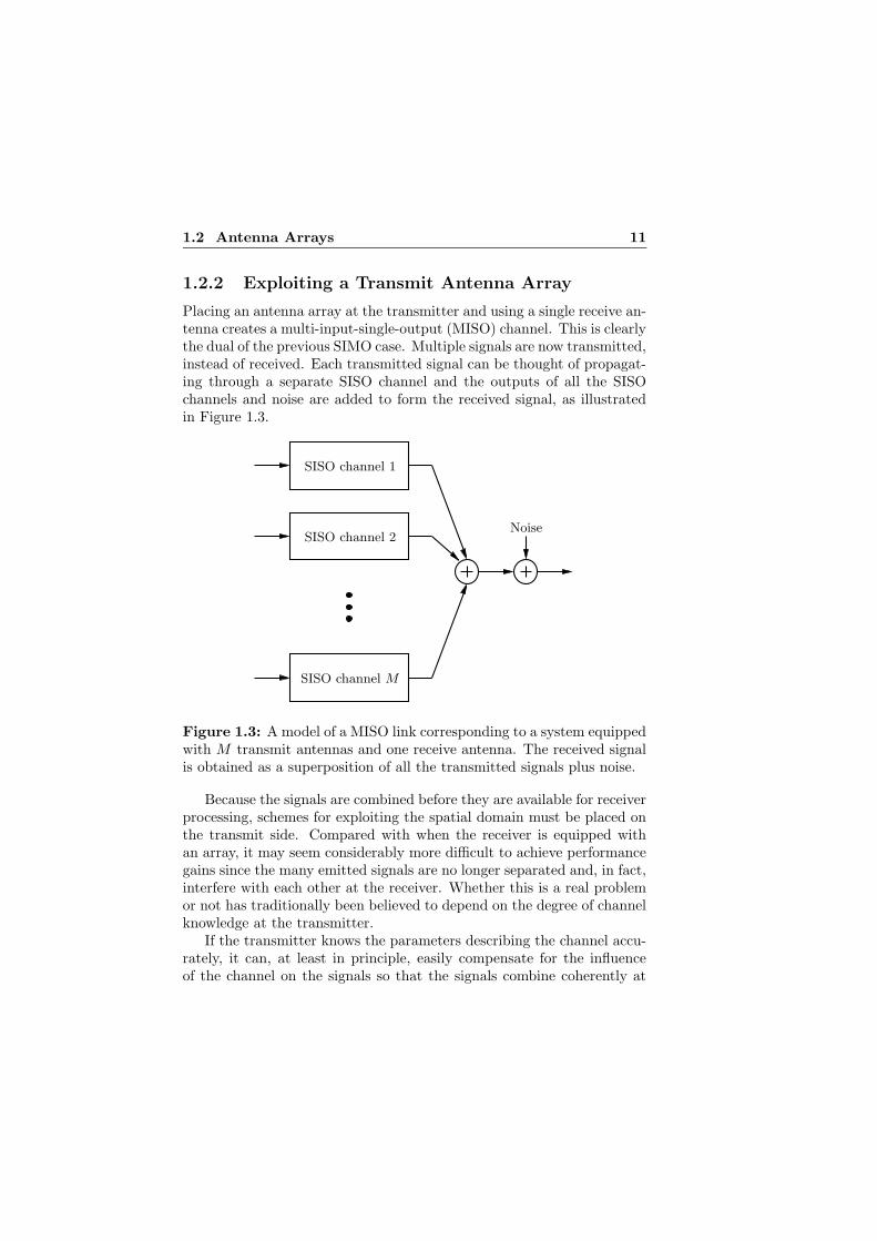
Placing an antenna array at the transmitter and using a single receive an-tenna creates a multi-input-single-output (MISO) channel. This is clearlythe dual of the previous SIMO case. Multiple signals are now transmitted,instead of received. Each transmitted signal can be thought of propagat-ing through a separate SISO channel and the outputs of all the SISOchannels and noise are added to form the received signal, as illustratedin Figure 1.3.
PSfrag replacements
SISO channel 1
SISO channel 2
SISO channel M
Noise
Figure 1.3: A model of a MISO link corresponding to a system equippedwith M transmit antennas and one receive antenna. The received signalis obtained as a superposition of all the transmitted signals plus noise.
Because the signals are combined before they are available for receiverprocessing, schemes for exploiting the spatial domain must be placed onthe transmit side. Compared with when the receiver is equipped withan array, it may seem considerably more difficult to achieve performancegains since the many emitted signals are no longer separated and, in fact,interfere with each other at the receiver. Whether this is a real problemor not has traditionally been believed to depend on the degree of channelknowledge at the transmitter.
If the transmitter knows the parameters describing the channel accu-rately, it can, at least in principle, easily compensate for the influenceof the channel on the signals so that the signals combine coherently at
12 1 Introduction
the receiver, thus avoiding interference. Hence, assuming the transmitterhas accurate channel knowledge, transmit antenna arrays are relativelystraightforward to exploit.
However, in the absence of channel state information, the transmit-ter has no way of knowing how the channel has affected the relativephases and time delays of the signals when they combine at the receiver.Channel knowledge at the transmitter is typically more difficult to obtainthan at the receiver. Because of these two factors, exploiting the poten-tial inherent in transmit antenna arrays has been viewed as difficult andhas consequently received rather limited interest. A classic solution thatavoids the use of channel information is to transmit the same signal onall antennas but with different carriers so that the signals do not over-lap in frequency [Jak94, p. 512]. The signals can then be separated atthe receiver by means of bandpass filtering and thereafter be combinedto obtain transmit diversity. Unfortunately, this comes at the price ofsignificant bandwidth expansion. It is only recently that more efficienttechniques coping with no channel knowledge have been developed.
Channel Knowledge at the Transmitter
When there is significant channel knowledge at the transmitter, some ofthe methods applicable when the array is placed at the receiver have di-rect counterparts on the transmit side. For example, the equivalent ofmaximum ratio combining on the transmit side is transmit beamforming[MM80]. In beamforming, scaled and phase shifted versions of the sameinformation carrying signal is transmitted from the different antennas insuch a manner that they add constructively at the receiver with the aimof maximizing the SNR. Beamforming in its simplest form correspondsto a purely spatial filter with the same coefficients as in maximum ratiocombining, i.e., the filter is matched to the channel coefficients. Thisconverts the original MISO channel into an artificial SISO channel. As-suming a flat fading scenario, the properties of the SISO channel are suchthat both the diversity and the array gain are of the same order as whatmaximum ratio combining with the same number of antennas provides.In other words, beamforming achieves all the spatial diversity the systemhas to offer. More general spatio-temporal filtering on the transmit sideis also possible [Koh98].
Beamforming changes the antenna pattern so that the radiated en-ergy is mostly confined to a narrow beam pointing in a certain direction.There is leakage of energy in other directions as well but it is small when
1.2 Antenna Arrays 13
PSfrag replacements
Transmitter
Receiver
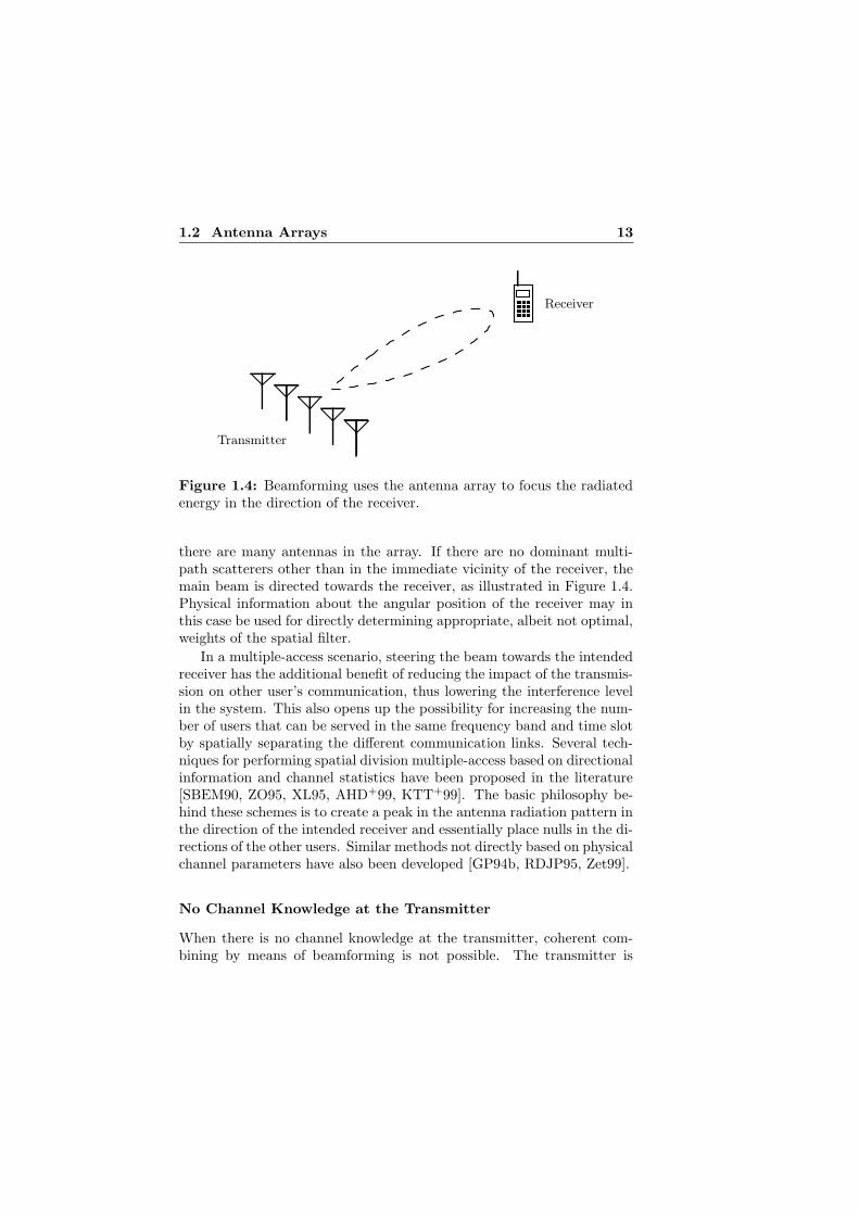
Figure 1.4: Beamforming uses the antenna array to focus the radiatedenergy in the direction of the receiver.
there are many antennas in the array. If there are no dominant multi-path scatterers other than in the immediate vicinity of the receiver, themain beam is directed towards the receiver, as illustrated in Figure 1.4.Physical information about the angular position of the receiver may inthis case be used for directly determining appropriate, albeit not optimal,weights of the spatial filter.
In a multiple-access scenario, steering the beam towards the intendedreceiver has the additional benefit of reducing the impact of the transmis-sion on other user’s communication, thus lowering the interference levelin the system. This also opens up the possibility for increasing the num-ber of users that can be served in the same frequency band and time slotby spatially separating the different communication links. Several tech-niques for performing spatial division multiple-access based on directionalinformation and channel statistics have been proposed in the literature[SBEM90, ZO95, XL95, AHD+99, KTT+99]. The basic philosophy be-hind these schemes is to create a peak in the antenna radiation pattern inthe direction of the intended receiver and essentially place nulls in the di-rections of the other users. Similar methods not directly based on physicalchannel parameters have also been developed [GP94b, RDJP95, Zet99].
No Channel Knowledge at the Transmitter
When there is no channel knowledge at the transmitter, coherent com-bining by means of beamforming is not possible. The transmitter is

14 1 Introduction
effectively blind since it cannot predict how the channel will affect thetransmission. Despite this fact, an antenna array may provide spatialdiversity of the same order as when there is perfect channel knowledgeor when the array is placed at the receiver.
Early attempts at exploiting multiple antennas for blind transmit-ters are focused on achieving spatial diversity. A common strategy isto convert the MISO channel into a synthetic SISO channel upon whichstandard scalar error-correcting codes can be used. Many ways to ac-complish that have been proposed in the literature.
In [HAN92, Wee93, KF97], phase shifted versions of the same infor-mation carrying signal are multiplexed to the different antenna elements.By making the phase shifts time-varying, a possibly static MISO channelis transformed into a fast fading SISO channel. The artificially createdtime-varying channel is used together with conventional time diversitymethods such as coding combined with interleaving [Pro95, p. 468]. Thus,spatial diversity is transformed into time diversity.
Another way of producing similar time-variations is to transmit ononly one antenna at a time and let the antennas take turn to transmit.The effective SISO channel coefficient thus alternates among the coeffi-cients in the MISO channel. Such a time division approach was proposedin [SW93], where a simple repetition code was used to exploit the result-ing temporal variations of the channel. Although the method providesdiversity, it comes at the expense of reduced data rate due to the repe-tition code. A more bandwidth efficient technique called delay diversitywas therefore also considered in the same paper.
Several other papers deal with delay diversity [Wit91, Wit93, Mog93,Win94, Win98]. The technique was originally proposed in [Wit91] and of-fers diversity by multiplexing time-delayed versions of the same informa-tion carrying signal onto the different antennas. The time delay increaseslinearly from no delay at the first antenna to some maximum delay atthe last antenna. Usually, the time delay differs with one symbol periodbetween two consecutive antennas. The result is a tapped delay line SISOchannel or, in other words, a frequency-selective channel. Decoding thereceived signal through the use of a maximum likelihood sequence esti-mator captures the frequency diversity of the synthetic SISO system. Abenefit of this strategy is that it does not waste waste bandwidth as in thetime division repetition code based approach in [Win98]. Other standardfrequency diversity methods are also applicable if bandwidth expansionis tolerated.
In the above blind diversity schemes, a coded stream of information

1.2 Antenna Arrays 15
bearing scalar symbols is spread over the antennas using various mul-tiplexing methods. The multiplexing techniques can all be seen as im-plementing special cases of a SIMO, possibly time-varying, linear spatio-temporal transmit filter. The resulting synthetic SISO link is representedby the compound channel from the input of the filter to the output ofthe single receive antenna. These ways of multiplexing are also com-monly referred to as linear precoding. Clearly, delay diversity is a specialcase of linear precoding with a simple time-invariant spatio-temporal fil-ter whose constituent single tap SISO filters implement the delays. Thetime division method corresponds to a strictly spatial time-varying filterwith the only non-zero coefficient placed at the currently transmitting an-tenna. Similarly, the frequency shifting approach corresponds to a purelyspatial filter with time-varying complex exponentials as coefficients.
Since also beamforming is equivalent to a spatial filter with complex-valued taps, frequency shifting implements a form of time-varying beam-forming where the direction of the beam thus varies with time and onlyby chance points towards the intended receiver. Consequently, the in-stantaneous SNR, and hence the overall performance, is typically muchlower than the maximum provided by conventional beamforming.
Information theoretic performance limits of all the mentioned blindlinear precoding schemes have been investigated in [NTW99] and com-pared with the performance of optimal non-linear vector coding. Inaddition, a random time-varying beamformer was proposed as a low-complexity method for exploiting some of the capacity of the system.The schemes mentioned so far all represent rather rudimentary and spe-cialized examples of spatio-temporal filtering. A broader class of linearprecoding techniques has been considered in [WT97].
It should be noted that encoding the data into a stream of scalarsymbols and thereafter applying any of the previously mentioned linearprecoding schemes is typically not optimal in a mutual information sensewhen there is no channel knowledge at the transmitter [NTW99]. Al-though such transmit structures permit simple decoding, they are notgeneral enough to achieve the maximum possible data rate that the sys-tem can offer. Since the MISO channel takes a vector-valued input, thechannel encoder needs to be designed specifically for vector (as opposedto scalar) symbols as output in order not to limit the potential data rate.Thus, for maximum performance, specifically developed vector codes needto be used that spread the information both in time and space.
Vector codes in transmit antenna array applications are more popu-larly known as space-time codes and have recently received considerable
16 1 Introduction
attention because of the high data rates and reliable communication theymay provide. Most of the literature on the design of space-time codesfocuses on a flat fading scenario in which the receiver is assumed to knowthe channel state parameters perfectly. The same code can usually beused regardless of the number of antennas at the receiver. The benefitsof deploying antenna arrays at both ends of the communication link willbe further discussed in the following section.
A systematic approach to designing space-time codes was pioneeredin [GFK96, GFBK99] where a design criterion was derived and used forverifying the performance of some simple space-time codes. Essentiallythe same design criterion was later derived in [TSC98] and shown to holdfor a number of different channel models. In the latter work, the nowpopular notion of space-time coding was introduced. Motivated by thedesign criterion, some examples of trellis codes realizing the full spatialdiversity potential of the system were proposed. In addition to diversity,the proposed space-time trellis codes give coding gain. The coding gainincreases with the number of states in the trellis, at the expense of higherdecoding complexity. These codes were basically handcrafted. Automaticdesign procedures for space-time trellis codes have been developed in e.g.[BBH00, Blu02] and used for obtaining more efficient codes than the onesfound in [TSC98].
An extremely simple yet novel space-time block code for two trans-mit antennas was given in [Ala98]. The code is commonly known as theAlamouti code after its inventor and has the appealing property that thetwo antenna signals are orthogonal in time (as well as in space) withoutthe bandwidth expansion normally associated with orthogonal signaling.The code is orthogonal in other ways too. Due to the orthogonal prop-erties of the code, the signals are easily separated at the receiver andmaximum possible spatial diversity gain is achieved. An additional andimportant advantage of this orthogonal space-time block (OSTB) code isthat optimal low-complexity decoding is possible. Corresponding codesfor up to eight transmit antennas was later given in [TJC99], where alsofurther theory was developed.
Other examples of OSTB codes are given in e.g. [GS01, SX03]. Aspointed out already in [TJC99], an OSTB code is a special case of a so-called linear dispersive space-time block code. That is, the code is linear interms of some constituent information carrying symbols. The individualcodewords can hence be obtained as a linear combination of these sym-bols where each symbol is weighted by a corresponding weighting matrix.By a clever choice of weighting matrices, OSTB codes arise. However,

1.2 Antenna Arrays 17
other weights are also certainly possible. In [HH02b], the weighting ma-trices were designed to maximize a channel capacity based performancecriterion. The resulting linear dispersive codes provide high reliable datarates if concatenated with suitable outer codes. Thanks to the linearstructure, it is possible to apply near optimal decoding techniques thatare more computationally efficient than the worst case of a full search[VH02, JMO03].
The space-time coding references mentioned so far all assume per-fect channel state information at the receiver. Non-coherent detec-tion scenarios corresponding to situations in which there is no chan-nel knowledge at the receiver have also been considered in several pa-pers. In [TAP98], it was shown that OSTB codes can be decoded with-out any channel knowledge at the price of some reduction in perfor-mance. Also, the classic concept of differential coding [Pro95] for non-coherent detection has been extended to the problem at hand, see e.g.[HS00, Hug00, TJ00, HH02a, GS02].
Another strategy for exploiting multiple transmit antennas is to useconventional scalar codes together with spatial interleaving. The ideais basically to introduce spatial redundancy by spreading the outputof a scalar encoder “evenly” over the different antennas. Transmis-sion schemes in this category include the well-known BLAST archi-tecture [Fos96], turbo [SD01] and trellis based techniques [RJ99]. Inthe latter work, orthogonal frequency division multiplexing (OFDM)[WE71, Cim85, Bin90] is used to handle a frequency-selective channelby dividing the bandwidth into narrow subbands creating a set of par-allel flat fading channels. This is a well-known technique for dealingwith frequency-selective channels and has also been used together withclassical space-time trellis codes in [ATNS98]. By utilizing time reversaltechniques, the concept of OSTB codes can be extended for this scenarioas well [LP00]. Space-time block codes for frequency-selective channelshave also been designed specifically for non-coherent receivers [GS03].
1.2.3 The Potential of Dual Antenna Arrays
Obviously, both sides of the communication link may be equipped withantenna arrays. The resulting multi-input-multi-output (MIMO) channelrepresents a natural extension of the previously described MISO case.Such dual antenna array systems offer more degrees of spatial freedom forthe spatio-temporal processing to exploit. In sufficiently rich multipathscattering environments, these extra degrees of freedom lead to a channel

18 1 Introduction
capacity substantially higher than when only a single antenna array isused [Tel95, FG98, RC98, RJ99], regardless of whether the transmitterknows the channel parameters or not.
The use of dual antenna arrays in rich scattering environments givesrise to a multiplicative effect that makes the channel capacity increaseessentially a constant integer factor faster with respect to the SNR thancomparable SISO, MISO or SIMO systems [FG98, RJ99]. The numericalvalue of the factor is given by the minimum of the number of antennasat the transmitter and receiver, respectively. Intuitively speaking, theMIMO channel broadens the channel in the sense that many parallel“data pipes” are available for the communication. The number of datapipes corresponds to the multiplicative factor mentioned above. Thisexplains the improvement in capacity compared with systems that donot use dual antenna arrays.
The encouraging capacity results exhibited by MIMO systems suggestthat reliable and high data rate communication may be accomplished inways that do not incur significant bandwidth expansion. Transmissionschemes for multiple transmit antennas generally work with dual antennaarray systems as well without modification, but with better performance.In fact, many of the space-time codes described above are designed withan arbitrary number of receive antennas in mind. Some transmissionschemes can however be greatly improved if they are specifically adaptedto the MIMO channel. For example, if the channel knowledge at thetransmitter is perfect, conventional beamforming unnecessarily limits thepossible data rates. Instead a related multi-dimensional type of beam-forming as in [RC98] is necessary in order not to lose capacity.
Investigations regarding MIMO channel capacity have been conductedfor several different scenarios. The classic MIMO capacity formula for flatfading channels with no channel knowledge at the transmitter and perfectchannel knowledge at the receiver was presented in [Tel95]. Therein, thecapacity gains possible in a Rayleigh fading scenario were illustrated andanalytical results provided. The potential for high data rates was furtherdemonstrated in [FG98] using the concept of outage capacity. The caseof perfect channel knowledge at the transmitter under the assumption ofconstant channel parameters was briefly considered in [Tel95] where itwas pointed out that traditional water-filling [CT91, p. 253] techniquesmay be employed. Works on frequency-selective channels treating thecases of perfect and no channel knowledge at the transmitter have beenreported in [RC98] and [RJ99], respectively. The MIMO channel capacitywhen both the transmitter as well as the receiver completely lack channel

1.3 Obtaining Channel State Information 19
state information (corresponding to a non-coherent detection scenario)was derived in [MH99] under the assumption of a flat fading scenario.
Most works on MIMO capacity and space-time coding primarily con-siders channel models that correspond to direct generalizations of stan-dard SISO [BD91, Bur96] and MISO/SIMO channel models [ECS+98].More advanced and perhaps more realistic channel models specificallydeveloped for MIMO systems are found in e.g. [SFGK00, GBGP02,KSP+02, WJ02].
1.3 Obtaining Channel State Information
As indicated by the previous discussion about antenna arrays, many tech-niques both on the transmit and receive side rely on channel state infor-mation. Due to the random and time-varying characteristic of the wire-less propagation medium, the parameters constituting the channel stateinformation need to be continuously estimated.
Channel estimation may be performed by exciting the system withsuitably chosen signals and studying the resulting output to deduce theparameters in the channel model. The model of the channel may be for-mulated in terms of physical parameters such as DOA, propagation pathdelays and gains [ECS+98] or in a more abstract form where for examplecoefficients of finite impulse response filters constitute the channel state.
The most common way to estimate the channel is through the use oftraining based methods where signals known to the receiver excite thechannel. Standard methods in estimation theory [Kay93] may then beutilized for determining the channel parameters. When there are multipleantennas on the transmit side, the choice of training sequences on thedifferent antennas becomes particularly critical in order to obtain goodchannel estimates [GFBK99].
Another approach is to use channel estimation methods which do notrely on knowing the transmitted signals. Such blind techniques identifythe channel solely based on received signals by utilizing the rich structuretypical of communication signals and channel models. A survey of somerecent blind methods is given in [TP98].
Regardless of whether blind or training based methods are used, theresulting channel estimates are directly available for receiver processing.Obviously, the estimates will not be perfect. Both noise and mismatchbetween the assumed model and the actual system introduce errors inthe channel state information.

20 1 Introduction
There are several ways in which channel estimates obtained at thereceiver can be used also for transmission purposes. When the systememploys duplex communication, the same device is both a transmitterand a receiver depending on the communication direction. Channel esti-mates based on reverse link data, as obtained in receive mode, can thenbe utilized also in the forward link, i.e., in the transmit mode. The twolinks in duplex communication are however usually separated either intime or frequency and this may severely degrade the quality of the chan-nel information in the transmit mode compared with the receive mode.
In time division duplex (TDD) systems, the forward and reverse linksare active on different non-overlapping time slots. Both communicationdirections use the same carrier frequency. As a result, assuming the du-plex time is short compared to the coherence time of the channel, theforward and reverse radio channels are the same. Due to this reciprocity,a channel estimate obtained in receive mode can be directly used in trans-mit mode, after taking into account that the transmit and receive filtersmay be different. On the other hand, if the duplex time is not shortenough, the channel may have changed considerable compared with thestate it was in when the channel estimate was obtained in the receivemode. In other words, the channel estimate is outdated, making thechannel state information available in the transmit mode much worsethan what the receive mode has access to. This discrepancy may to someextent be lessened by utilizing the temporal correlation of the channel forestimating the current channel based on the outdated channel informa-tion [DHSH00].
The same strategy of utilizing a channel estimate obtained in thereverse link for forward link processing is applicable also in frequencydivision duplex (FDD) systems, under certain conditions. Different car-rier frequencies are now used in the two communication directions. Ifthe frequency separation is sufficiently small compared with the coher-ence bandwidth of the channel, the forward and reverse link channels areessentially the same and just as for the above TDD case, the same chan-nel estimate can be used directly in both the transmit and the receivemode if the differences in transmit and receive filters are compensatedfor. Frequency correlation properties of the channel may now be usedfor improving the estimation accuracy in case the frequency separationis not sufficiently small.
An alternative and perhaps better approach when the frequency sep-aration in FDD is too large is to estimate the state of the forward channelbased on physical parameters such as DOA that may be assumed to be

1.3 Obtaining Channel State Information 21PSfrag replacements
Transmitter Receiver
Feedback link
Channelinformation
......
Figure 1.5: The receiver informs the transmitter about the channel viaa dedicated feedback link.
invariant to the carrier frequency. Another completely different strategywhich is suitable for FDD systems is to equip the system with a dedicatedwireless feedback link that conveys estimates of channel parameters fromthe receiver to the transmitter [GP94a, HP98]. The setup is illustratedin Figure 1.5.
There are however problems also with a feedback approach. Obvi-ously, it takes time to transport the channel estimates over the feedbacklink. In the mean time, the time-varying channel may have changed somuch that the feedback output has become outdated. To avoid such dif-ficulties, the feedback delay must be small in comparison with the coher-ence time of the channel. In typical land-mobile applications, this meansthat the channel information at the transmitter needs to be updated ata high rate.
The requirement of a high update rate and the need for a spectrallyefficient system in which not too much bandwidth is wasted on the feed-back link unfortunately represent two conflicting goals. One way to ob-tain a reasonable comprise between these two goals is to limit the datarate necessary to maintain a high update rate by quantizing the chan-nel parameters heavily before they are fed back to the transmit side. Adrawback with this solution is of course that quantization errors nowplague the channel information at the transmitter. Note also that thecommunication over the feedback link potentially suffers from bit-errorsdue to the non-perfect nature of the wireless feedback channel. To makematters worse, the requirement on short feedback delay typically pre-vents the use of advanced channel coding in the feedback link. The errorrate can consequently be quite high, adding another significant sourceof errors. Thus, estimation noise at the receiver, feedback delay, coarsequantization and bit-errors introduced by the feedback channel are alllikely to contribute in degrading the quality of the channel information

22 1 Introduction
at the transmitter. Despite these shortcomings, providing channel feed-back is often worthwhile as evidenced by the use of a feedback link in theclosed-loop transmit diversity mode of the WCDMA system [3GP02b].
1.4 Imperfect Channel Knowledge
Most transmission methods and performance analyses for multiple trans-mit antennas are developed under either of the two extreme assumptionsof perfect channel knowledge or no channel knowledge at the transmitter.Classical beamforming by means of a spatial filter matched to the chan-nel falls in the former category. So does the transmission method andcapacity analysis for MIMO systems in [RC98]. Basically the entire fieldof space-time coding belongs to the latter category where channel knowl-edge at the transmitter is totally excluded from the development. Thewell-known MIMO channel capacity works in [Tel95, FG98] also focus onthe same extreme case.
However, as should be clear from the previous section, it is often possi-ble to obtain channel information at the transmitter. The problem is thatit is typically far from being perfect. Thus, in practice, neither of the twoextreme views are correct. This issue has to some extent been addressedin [Wit95] where beamforming weights are determined in such a mannerso as to reduce the devastating impact of defective channel information.In another work [HP98], a method for determining beamforming weightsbased on heavily quantized channel feedback is proposed.
Information theoretic investigations of how the quality of the availablechannel information influences the properties of optimal signaling showthat, if the quality is sufficiently low, conventional beamforming is notoptimal in a mutual information sense [NLTW98]. A later and relatedwork gives an analytical expression on the threshold where beamformingis no longer optimal in terms of channel capacity [VM01].
The reason why beamforming performs badly in situations of lowchannel knowledge quality is because of the one-dimensional nature ofthe resulting transmission – the emitted energy is focused in only onedirection determined by defective channel information. When the qualityof the channel information is low, such a single beam transmission schemeoften emits energy in the wrong direction. In the extreme case of nochannel knowledge, it should be clear that a better strategy is to spreadthe energy uniformly in all directions. This is what conventional space-time codes aim for.

1.4 Imperfect Channel Knowledge 23
One way to take channel knowledge into account is to use a trans-mit weighting matrix for adapting the output of a fixed conventionalspace-time encoder. The transmit weighting is determined solely fromthe available channel information while the output of the fixed space-timeencoder depends only on the data to be communicated. In contrast tobeamforming, such a transmission structure allows energy to be emittedin several directions at the same time, which is necessary if the channelstate information is poor. Concentrating all the emitted energy in a singledirection is also possible if the circumstances should require it. Separatespace-time coding and transmit weighting in this manner represents anappealing and flexible transmission structure. The structure is even moreinteresting in view of the fact that under certain conditions it is optimalin the sense of preserving the capacity of the MIMO system [SJ03].
By using OSTB codes in the fixed space-time encoder, simple andefficient transmit weighting schemes were developed in [JO99, JSO00,JSO02a]. These transmission methods/structures will in the present workbe referred to as weighted OSTBC, where OSTBC stands for orthogo-nal space-time block coding. The same weighted OSTBC transmissionschemes have later been proposed and investigated in [ZG02a, ZG02b]for a special case of the setup considered in [JO99, JSO00, JSO02a].Weighted OSTBC may also be extended to handle quantized channelinformation obtained from a non-ideal feedback link [JS00, JS01]. Ananalysis on the diversity order potentially provided by separate OSTBcoding and transmit weighting in case of quantized feedback is found in[LGSW02].
Another way of utilizing available channel knowledge is to completelyavoid the use of conventional space-time codes and instead consider thedesign of entirely new space-time codes that are allowed to depend on thechannel information. Such an approach has been explored in [JSO02b]for the design of unstructured space-time block codes which exploit quan-tized channel feedback. Compared to the above transmit weighting meth-ods, the unstructured nature of the code gives more degrees of freedomin determining appropriate signals to transmit. Consequently, the per-formance increases but at the expense of substantially higher decodingcomplexity.

24 1 Introduction
1.5 Outline and Contributions
This thesis investigates performance limits and develops transmissionmethods and code designs for a flat fading MIMO wireless communicationlink where the transmitter has access to possibly imperfect channel sideinformation while the receiver knows the channel perfectly. An outline ofthe remaining chapters in the thesis is presented below, where also someof the contributions are mentioned.
Chapter 2
In this chapter, an expression for the channel capacity of the system understudy is presented and subsequently analyzed. The capacity expressionapplies to a scenario in which the channel and the channel side informa-tion may be modeled as jointly stationary and ergodic random processes,subject to certain additional assumptions. A block fading scenario wherethese processes are piecewise constant in time is shown to also be handledby the same capacity expression. The corresponding block fading systemmodel forms the basis of the models used in later chapters.
There are several contributions in the chapter in addition to present-ing an expression for the channel capacity. It is pointed out that thecapacity expression, originally derived for a scenario where power con-trol is allowed, reduces to previously used expected mutual informationbased performance measures, if power control is prohibited. This is im-portant since it establishes the validity of these widely used performancemeasures. Another important result is that separate space-time cod-ing and transmit weighting is a capacity achieving transmitter structure.Weighted OSTBC is a simple special case of this structure and shown tobe optimal in the case of two transmit antennas and one receive antenna.The latter result provides motivation for the low-complexity weightedOSTBC transmission scheme proposed in later chapters. The capacityexpression turns out to often be difficult to evaluate. Procedures fornumerically computing the capacity are therefore considered and a the-ory concerned with symmetrical properties of quantized channel feedbackis introduced. Numerical examples illustrate the capacity gains due tochannel side information at the transmitter in a spatially uncorrelatedRayleigh fading scenario.
Parts of this material have been published as
M. Skoglund and G. Jongren. On the capacity of a multiple-antennacommunication link with channel side information. IEEE Journal
1.5 Outline and Contributions 25
on Selected Areas in Communications, 21(3):395–405, April 2003.
This paper contains, among other things, the proof of the capacity for-mula, which the development in the chapter is based on. Even thoughthe proof is important we have chosen to omit it in the development tofollow and instead focus on the consequences of the capacity formula.
Chapter 3
In this chapter, the system model used for the remainder of the the-sis is introduced. Like in parts of the previous chapter, a block fadingscenario is considered where the channel and the channel side informa-tion are modeled as constant during a block of samples and then varyfrom one block to another. An important difference compared with ourearlier information theoretic investigations is that the channel coding ishenceforth assumed to be performed for one fading block at a time, i.e.,the transmitted codewords do not extend over possibly different channelrealizations.
In addition to a system model, three different classes of space-timeblock codes that can take channel side information into account are de-scribed for later reference. These three classes, mentioned in order ofincreasingly restrictive structure, correspond to unstructured codes, lin-ear dispersive codes and weighted OSTBC. Whereas unstructured andlinear dispersive codes are previously known code types, weighted OS-TBC was originally proposed in the works that form the basis of thisthesis. Hence, the weighted OSTBC structure represents an importantcontribution.
Each code is represented by a set of codeword matrices. The threecode classes differ in the kind of structural constraints that are imposedon the matrices. The structure of weighted OSTBC is so restrictive thatit is perhaps better labeled as a transmission structure rather than acode structure. Both notions will be used interchangeably wherever ap-propriate. However, thinking in terms of a code makes weighted OSTBC,together with the other structures, fit naturally within a common frame-work of channel side information dependent space-time block codes. Theframework serves to emphasize that the code design (or transmission)procedures developed in subsequent chapters are easily modified to han-dle the construction of any of these code classes.

26 1 Introduction
Chapter 4
This chapter deals with code design in the presence of possibly imperfectchannel side information. The non-ideal nature of the latter is modeledby assuming that the channel conditioned on the side information is com-plex Gaussian [Kay93, p. 507] distributed. A major contribution is thedevelopment of a new performance criterion for space-time codes thattakes channel knowledge at the transmitter into account. The perfor-mance criterion is based on an upper bound on the pairwise codeworderror probability conditioned on the available side information.
Another major contribution is the use and analysis of the performancecriterion for code design. An outline of code design procedures for all ofthe three code classes is given. Particular attention is thereafter directedto our proposed weighted OSTBC structure and how to reduce the com-putational complexity when designing the transmit weighting matrix. Itturns out that the resulting transmission scheme can be seen as a seamlesscombination of conventional OSTB coding and beamforming, where thequality of the channel side information determines whether the transmit-ted output is more like that of the former or latter method. Numericalresults for a spatially uncorrelated Rayleigh fading scenario illustrate thatsignificant gains compared with both beamforming and OSTBC are pos-sible. In particular, the scheme provides robustness against impairmentsin the channel side information in contrast to conventional beamformingwhich suffers severely from such errors.
The parts about the pairwise error probability and weighted OSTBChave been published as
G. Jongren, M. Skoglund, and B. Ottersten. Combining beamform-ing and orthogonal space-time block coding. IEEE Transactions onInformation Theory, 48(3):611–627, March 2002.
and have also appeared in
G. Jongren and B. Ottersten. Combining transmit antenna weightsand orthogonal space-time block codes by utilizing side informa-tion. In Proc. 33th Asilomar Conference on Signals, Systems andComputers, October 1999.
G. Jongren, M. Skoglund, and B. Ottersten. Combining transmitbeamforming and orthogonal space-time block codes by utilizingside information. In Proc. First IEEE Sensor Array and Multi-channel Signal Processing Workshop, March 2000.

1.5 Outline and Contributions 27
Chapter 5
In this chapter, the use of weighted OSTBC based on quantized channelside information is considered. The channel side information is obtainedfrom the receiver via a dedicated feedback link. Quantization errors, feed-back delay and feedback channel bit-errors are all assumed to plague theside information. Techniques related to the field of channel optimizedvector quantization (COVQ) [FV91] are used for determining how thechannel information can be quantized into a small number of bits whiletaking the error sources into account. The bits are conveyed to the trans-mitter where they are decoded into an estimate of the current channelrealization.
Two different ways of measuring the error between the true channeland the channel estimate are used in the design of the quantizer. Inthe first approach, the error is defined based on the differences betweenthe true and estimated channel coefficients, similarly to as in standardminimum mean-square error (MMSE) estimation. Such an error measureis easy to analyze but requires a rather large number of bits to performwell. This motivates the second more efficient approach of separatelymeasuring relative phase and amplitude errors.
The two types of feedback links can be used with any of the threecode classes or with other transmission schemes. The presentation in thechapter is however entirely focused on the use of weighted OSTBC. Thetransmit weight design procedure described in the preceding chapter isdirectly applicable if the first feedback link type is used. For the case ofthe second feedback link type, the design procedure needs to be modi-fied. A heuristic method for doing this is presented. Simulation resultsshow that the resulting transmission scheme compares favorably withboth beamforming as well as conventional OSTB coding. In particular,robustness against quantization errors, feedback delay and bit-errors isachieved.
Parts of this chapter have been published in
G. Jongren and M. Skoglund. Utilizing quantized feedback infor-mation in orthogonal space-time block coding. In Proceedings IEEEGlobal Telecommunications Conference, November 2000.
G. Jongren and M. Skoglund. Improving orthogonal space-timeblock codes by utilizing quantized feedback information. In Pro-ceedings International Symposium on Information Theory, June2001.
28 1 Introduction
and the whole chapter, with some minor modifications, has been submit-ted as
G. Jongren and M. Skoglund. Quantized feedback information inorthogonal space-time block coding. Submitted to IEEE Transac-tions on Information Theory.
Chapter 6
This chapter presents another approach to tackle the problem of designingspace-time codes that take advantage of quantized channel side informa-tion. Instead of relying on heuristic modifications of a design procedureoriginally derived for non-quantized side information, a new performancecriterion specifically tailored to quantized feedback is derived. The ob-tained performance criterion turns out to be quite similar in structureto the previous criterion. Hence, it can be used together with the codedesign procedures described in earlier chapters.
To illustrate the use of the new performance criterion, the designof unstructured codes, linear dispersive codes and weighted OSTBC isconsidered, with the primary focus on the first type of code. Attention isnow limited to a scenario in which the feedback link does not suffer frombit-errors and where the channel information is quantized using a specificfeedback scheme known as partial phase combining [HP98]. However, thedesign methods we propose are easily applicable to other types of feedbackschemes and can be generalized in a straightforward manner to deal withthe effects of feedback channel bit-errors.
Properties that optimal unstructured codes must possess are derivedand tables of code design results are provided. In particular, an exampleof an unstructured four codeword code that outperforms, even withoutany channel knowledge, the well-known Alamouti OSTB code is provided.
Some linear dispersive codes are also constructed. An interesting ob-servation is that the resulting codes are essentially equivalent to OSTBcodes, in the case of no channel knowledge. In addition, a design proce-dure for weighted OSTBC is implemented.
The concept of symmetric feedback again turns out to be useful forreducing computational complexity. Simulation results show that theconstructed codes outperform both OSTB coding and beamforming evenin the extreme cases of no or perfect channel knowledge.
Contributions in the chapter include the development of the perfor-mance criterion, the code design methods and the subsequent analysis.Some parts of this material have been published in

1.6 Future Work 29
G. Jongren, M. Skoglund, and B. Ottersten. Utilizing partial chan-nel information in the design of space-time block codes. In Proc. 5thInternational Symposium on Wireless Personal Multimedia Com-munications, October 2002.
while the parts pertaining to unstructured codes have been submitted as
G. Jongren, M. Skoglund, and B. Ottersten. Design of channelestimate dependent space-time block codes. Submitted to IEEETransactions on Communications.
1.6 Future Work
The work in this thesis leave several issues open for future research. Boththe information theoretic analysis and the code design methods can beextended in a number of ways. Some extensions are relatively straight-forward while other require substantial effort.
The information theoretic investigations in Chapter 2 are based on asingle capacity expression that is more versatile than what the presentstudy may indicate. It is for example possible to broaden the scope of thework to include more realistic fading scenarios and/or study the effectsof channel side information impairments other than quantization errors.Both numerical and analytical results would be useful in such studiesfor providing further insight into the problem. Feedback delay may bemodeled as in [NLTW98] and the impact on performance examined. Bit-errors introduced by a noisy feedback channel is another area that isinteresting to investigate. The gains provided by the use of power controlare also worthwhile to examine in more detail. A potential problemwith these extensions is however that they typically further complicatenumerical evaluation of the capacity expression. Thus there is a needfor more efficient optimization procedures than those presented herein.Another area to explore is the use of the capacity expression as a criterionfor the design of codes. Similar techniques as in [HH02b] can then be usedfor obtaining encoder structures that maximize the capacity expression.
The work concerning methods for code design leaves plenty of top-ics for future research. Perhaps the most obvious extension is to de-velop design methods specifically for a frequency-selective channel. Oneway to handle this essentially within the present framework is to useOFDM for converting a frequency-selective channel into a set of paral-lel flat fading MIMO channels. The methods developed herein can then

30 1 Introduction
be applied separately for each MIMO channel. However, for maximumperformance, techniques for jointly dealing with all the parallel channelsneed to be developed. An alternative approach which avoids OFDM isto use single-carrier transmission and instead more directly deal with anon-flat channel in both the performance criterion as well as the designprocedures, similarly to as in [GS03].
The code design methods all rely on a power constraint that corre-sponds to a scenario without power control. It is however possible toinclude power control into the design procedure by relaxing this con-straint, albeit at the expense of increased computational complexity. Inscenarios with quantized side information, the design is performed off-lineand the additional complexity may be tolerable. Power control can evenbe combined with variable rate coding so that the data rate is adaptedto the channel conditions via the available channel side information.
In this thesis, the code design is conducted separately from the designof the feedback link. However, since they both depend on each other,the code and the feedback link should be designed jointly for maximumperformance. An outline on how to perform such a joint design is given inour work in [JSO02b]. Numerical procedures remain to be implementedand the properties of the resulting codes and feedback links need to befurther investigated.
Another area which receives limited attention in this thesis is that ofmultiple-access and how to mitigate the total interference in a wirelessnetwork. In the literature, there are methods for performing global opti-mization of beamforming weights so that the coupling between differentcommunication links is kept as small as possible while meeting certainquality of service constraints [RFLT98, BO02]. Similar techniques maybe possible to apply for transmitter adaption based on the more generalweighted OSTBC structure. By modeling the interference from otherusers as Gaussian with some spatial color, the performance criteria de-veloped in the present work can easily be extended to take also this kindof disturbance into account. It is however still an open question if it ispossible to develop sufficiently efficient numerical procedures for jointlydetermining the transmit beamforming weights of all users in the system.
Finally, the methods need to be evaluated under more realistic condi-tions. Channel estimation errors also at the receiver should for examplebe considered. The impact of a continuously time-varying channel (asopposed to the present block fading assumption) should also be exam-ined. Preliminary investigations indicate that the methods can be madeto cope quite well with such common deviations from the idealized system

1.6 Future Work 31
model considered herein. Nevertheless, much further work is required tofully investigate all aspects of this issue.


Chapter 2
Capacity Results
This chapter considers a MIMO wireless communication system with pos-sibly imperfect channel side information at the transmitter and investi-gates performance limits from an information theoretic perspective. Thechannel and the channel side information are modeled as jointly station-ary and ergodic random processes. A formula for the channel capacity,valid under certain additional assumptions, is given and used for gaininguseful insights about the problem by applying it to different scenarios.The proof of the capacity formula is not included herein, but can be foundin our work in [SJ03].
It turns out that separate space-time coding and transmit weightingis an optimal capacity achieving transmitter structure. In the case of twotransmit antennas and one receive antenna, an OSTB encoder followedby a transmit weighting is also shown to achieve capacity. This providesmotivation for the weighted OSTBC transmission scheme developed inlater chapters. Attention is in particular devoted to a scenario in whichthe side information consists of quantized channel information obtainedfrom the receiver via a feedback link. This setup is closely related to theclosed-loop transmit diversity mode in the WCDMA system, making thecorresponding capacity results interesting from a practical point of view.Numerical examples for a spatially uncorrelated flat Rayleigh fading sit-uation illustrate that the use of channel knowledge at the transmitterresults in considerable gains compared with when channel knowledge isnot utilized.

34 2 Capacity Results
2.1 Introduction
Information theoretic studies show the high data rates that wirelessMIMO systems may offer [Tel95, FG98, RC98, RJ99]. The recent de-velopment of space-time codes [GFBK99, TSC98, TJC99] provides themeans for exploiting the potential of the MIMO channel in practice.
In the literature, different capacity measures have been used depend-ing on the scenario under consideration. The classical MIMO capacityformula for a scenario in which the channel fades in an ergodic manner isgiven in [Tel95]. With a slow block-wise channel fading scenario in mind,the concept of outage capacity is used in [FG98] to illustrate the extraor-dinarily high data rates that are possible when both the transmitter andthe receiver are equipped with antenna arrays. Both these works rely onthe assumption of perfect channel state information at the receiver whilethe transmitter does not know the channel. In contrast, a non-coherentdetection scenario is considered in [MH99], where the capacity is derivedunder the assumption that neither the transmitter nor the receiver knowthe channel. The case of perfect channel knowledge at both the transmit-ter and the receiver has also been treated. Assuming a constant channel,the corresponding capacity is investigated in [RC98]. In [BCT01], thefocus is instead on block-wise channel fading and outage capacity as aperformance measure.
The works mentioned so far all take on the extreme view that thetransmitter either knows the channel perfectly or not at all. However, asdiscussed in Section 1.3, channel side information at the transmitter, ifavailable, is typically far from being perfect in practice. Even if the sideinformation about the channel is not perfect, it may still help in increasingthe performance of the system. This provides motivation for the workpresented in this chapter that introduces and analyzes a capacity formulathat is applicable also to the more realistic scenario of a transmitterhaving access to imperfect channel state information.
Most of the presentation is devoted to the case when the output poweris allowed to fluctuate with the channel side information, correspondingto a system with power control. However, scenarios without power controlare also treated to some extent. The capacity formula is based on theassumption of an ergodic flat fading scenario in which the channel sideinformation at the transmitter may be non-perfect while the receiverknows both the channel as well as the channel side information availableat the transmitter. The assumptions about the receiver cover situationswhen the receiver can estimate the channel parameters accurately and
2.1 Introduction 35
uses a feedback link, with a corresponding ideal feedback channel thatdoes not introduce bit-errors, to convey heavily quantized versions of thechannel parameters to the transmitter. When the receiver’s knowledge ismore restrictive, our capacity results represents an upper bound on theachievable performance. Although the focus is on flat fading scenarios, afrequency-selective channel may be handled within the present frameworkby using multicarrier techniques such as OFDM [WE71, Cim85, Bin90]to convert the channel into a set of parallel flat fading channels.
Previous information theoretic studies concerned with communica-tion links with possibly imperfect channel side information and multipletransmit antennas are surprisingly scarce.
In [NLTW98], a system with one receive antenna in a Rayleigh fadingscenario is considered. The channel side information at the transmitterand the channel are assumed to be jointly Gaussian distributed. Mutualinformation averaged over the ensemble of channel and side informationrealizations is used as performance measure. It is assumed that this mea-sure gives the maximum rate of reliable communication but it is not clearwhether it actually corresponds to the capacity of some channel. This isin contrast to the present work which establishes an expression for thetrue channel capacity under the assumption of a more general fading sce-nario. As discussed later in this chapter, when the scenario is specializedinto the one used in [NLTW98], our capacity expression reduces to thesame expected mutual information based performance measure as in thatpaper. Consequently, the performance measure in [NLTW98] constitutesa channel capacity and is hence well motivated.
Another work dealing with wireless MISO systems and channel sideinformation is presented in [VM00]. In this work, so-called mean orcovariance feedback is considered, referring to the fact that the secondorder statistics of the channel now play the role of the side informationat the transmitter. With an underlying assumption of Gaussian channelfading, this in turn determines the stationary marginal distribution ofthe channel fading. Based on the classical MIMO capacity expressionin [Tel95], optimal transmission strategies are derived. The use of theclassical MIMO capacity expression implies a scenario in which the sideinformation is static and the channel is time-varying in an ergodic fashion.In other words, the transmitted signals should experience all possiblechannel realizations while the side information remains the same. Thismay be a reasonable assumption in scenarios were the side informationis updated very slowly compared with the coherence time of the channelfading. However, it is not an accurate model for the important case when
36 2 Capacity Results
a feedback link is used for real-time tracking of channel variations. Ourwork, on the other hand, includes both scenarios as special cases sincethe side information is allowed to be time-varying.
The capacity of a communication link with possibly imperfect channelside information has been studied in other previous works as well but thenwith the focus on SISO systems. For example, in [CS99], the capacity of aSISO link was derived for the case when there is channel side informationat the transmitter while the receiver knows a quantity corresponding tothe instantaneous SNR. The channel gain was assumed to be positive andassumed to fade in an ergodic fashion. A class of general discrete systemswas also investigated. In [DN02], a related multiple-access scenario wasconsidered. Other examples of works dealing with SISO links and channelside information, perfect as well as non-perfect, include [Sha58, Sal92,GV97, Vis99].
The main contribution of the present work is the development andstudy of an expression for the capacity of a MIMO system in which thetransmitter has access to channel side information. A result of partic-ular importance is the conclusion that separate space-time coding andtransmit weighting is optimal in the sense that it is a capacity achievingencoder structure. In this structure, the transmit weighting depends onlyon the side information while the space-time encoder uses a fixed code-book which is independent of the side information. It is also shown thatfor the case of two transmit and one receiver antenna, such a capacityachieving structure can be implemented using an OSTB code, giving riseto the previously mentioned weighted OSTBC transmission structure.This optimality in a capacity sense provides motivation for the weightedOSTBC transmission scheme proposed in later chapters. Numerical eval-uation of the capacity formula is in the general case non-trivial since itinvolves solving a difficult optimization problem. Therefore, optimiza-tion procedures are discussed and a theory about so-called symmetricfeedback is developed. By utilizing the symmetric feedback theory, com-puting the capacity becomes feasible in some cases when quantized sideinformation is available. Quantized side information typically arises insituations where a feedback link is used for providing channel informationto the transmitter. Assuming spatially uncorrelated flat Rayleigh fadingand one receive antenna, numerical results on the capacity are presented.Motivation for the setup under consideration is provided by the similaritywith the closed-loop transmit diversity mode of the WCDMA system.
The chapter is organized as follows. The system model is describedin Section 2.2. An expression for the capacity of the described system

2.2 System Model 37
is given in Section 2.3, where also the structure of a capacity achiev-ing encoder is discussed. Furthermore, extensions to block-wise channelfading scenarios are also presented. In Section 2.4, the extreme casesof no and perfect channel knowledge at the transmitter are consideredand the capacity expression is shown to then reduce to previously knownexpressions. An alternative capacity achieving structure is presented inSection 2.5, where it is proved that weighted OSTBC is optimal for thecase of two transmit antennas and one receive antenna. Computationof the capacity is treated in Section 2.6, where the symmetric feedbackconcept is used to significantly simplify the problem. Finally, numericalresults on the capacity are given in Section 2.7.
2.2 System Model
Consider the symbol sampled and complex baseband equivalent model ofa wireless narrow-band MIMO communication system depicted in Fig-ure 2.1. There are M transmit antennas, N receive antennas and ndenotes the integer-valued sample index. The frequency-nonselectivefading MIMO channel at discrete time instant n is represented by theN×M matrix H(n) with complex-valued elements Hkl(n), k = 1, · · · , N ,l = 1, · · · ,M , where Hkl(n) represents the channel between the lth trans-mit and the kth receive antenna.
PSfrag replacements
......
Space-Time
EncoderReceiver
H(n)︷ ︸︸ ︷
ζ(n)ζ(n)
H(n)
M N
c(n) x(n)
Figure 2.1: System model.
Channel side information is available at the transmitter. The sideinformation comes in the form of a time-varying vector ζ(n) which isstatistically related to H(n) in the sense that ζ(n) and H(n) areassumed to be jointly stationary and ergodic random processes. A space-time encoder maps the message to be transmitted and the side informa-tion into M parallel streams of channel symbols by choosing a codeword

38 2 Capacity Results
to transmit out of a set of codewords in a codebook. The codebook cor-responds to the channel code. The channel symbols at time instant n arerepresented by the output vector
c(n) ,[c1(n) c2(n) · · · cM (n)
]T, (2.1)
which is assumed to satisfy the power constraint
E[‖c(n)‖2] = P , (2.2)
where ‖·‖ denotes the usual vector or spectral matrix norm [HJ96, p. 295]and E[·] is the expectation operator. Here, (·)T represents the transposeoperator, , denotes “equality per definition” and cl(n) is a potentiallycomplex-valued channel symbol transmitted on the lth antenna at timeinstant n.
Adaptation of the transmission to variations in the channel conditionsis facilitated by the assumption of an encoder output that is allowed todepend on past and present side information. In other words, c(n) isa function of ζ(k)n
k=−∞ (causal side information), in addition to itsdependence on the message to be communicated. The resulting informa-tion carrying signals are transmitted over the wireless channel, picked upby the receiver’s antenna array and thereafter filtered and symbol sam-pled to produce the received signals. The complex baseband equivalentreceived signals are represented by the vector
x(n) ,[x1(n) x2(n) · · · xN (n)
]T, (2.3)
where xk(n) is the output from the kth antenna at time n. Decodingat the receiver is performed under the assumption that both the channelas well as the side information are known at the receiver, as indicatedin the figure. Channel state information at the receiver may in practicebe obtained by estimating the channel based on, for example, a trainingsequence. The side information is in some cases implicitly known at thereceiver while in other cases it also needs to be estimated. An exampleof the former case is when the side information ζ(n) is a deterministicfunction of the channel H(n), such as in a system where H(n) is quan-tized at the receiver and then conveyed to the transmitter via a feedbacklink that does not introduce bit-errors.
The signal output from each receive antenna is a weighted superposi-tion of the transmitted signals, corrupted by additive noise. Hence, the

2.2 System Model 39
output from the kth receive antenna can be written as
xk(n) =M∑
l=1
Hkl(n)cl(n) + ek(n) , (2.4)
where ek(n) represents the additive noise. By combining (2.1), (2.3), and(2.4), the received signal vector can be written as
x(n) = H(n)c(n) + e(n) , (2.5)
where the noise term
e(n) ,[e1(n) e2(n) · · · eN (n)
]T
is assumed to be generated from a zero-mean, temporally white, complexGaussian1 random process e(n). The processes e(n), (H(n), ζ(n))and the message to be transmitted are all assumed to be mutually inde-pendent. The spatial color of the noise is given by the covariance matrixE[e(n)e(n)∗] , Ree, where (·)∗ denotes the complex conjugate transposeoperator. Spatially white noise is usually a good model for thermal noisewhile colored noise can be used to model interference from other users ina cellular network.
2.2.1 An Additional Assumption
For the above system, an upper bound on the data rate possible for essen-tially error-free communication (as the processing block length tends toinfinity) is derived in our work in [SJ03]. However, as pointed out therein,to proceed and obtain a compact capacity expression, which shows thatthe upper bound is in fact attainable, makes it necessary to impose anadditional constraint regarding the statistical relation between the sideinformation and the channel. Similarly to as in the related SISO workin [CS99], the required constraint is the assumption that ζ(k)n−1
k=−∞,
ζ(n), H(n) form a Markov chain ζ(k)n−1k=−∞ – ζ(n) – H(n). In other
words,
p(ζ(k)n−1
k=−∞|ζ(n),H(n))
= p(ζ(k)n−1
k=−∞|ζ(n)), (2.6)
1If desired, the complex Gaussian assumptions found throughout this work (andindeed the whole thesis) may all be generalized to the corresponding Gaussian as-sumptions, without resulting in nothing but straightforward modifications of the de-velopment.
40 2 Capacity Results
where p(·) denotes a probability mass/density function (PMF or PDF,respectively). The above condition means that H(n) gives no furtherknowledge about the past side information ζ(k)n−1
k=−∞ when ζ(n) isknown.
2.2.2 Scenarios Satisfying the Assumptions
It should be clear that the major part of the system model describedabove is reasonable in many scenarios. However, the additional assump-tion in (2.6) seems rather arcane and does in fact significantly limit thefield of application. Despite this, there are a number of scenarios encoun-tered in practice in which the entire system model is applicable. Below,examples of such scenarios are given.
No Channel Knowledge
The extreme case of no channel knowledge at the transmitter can bemodeled by assuming that ζ(n) and H(n) are mutually independent.Clearly, (2.6) is satisfied and hence the present work includes this commonscenario as a special case.
Perfect Channel Knowledge
For the other extreme of perfect channel knowledge, the side informationis equal to the channel, or more precisely, ζ(n) = γ(H(n)), where γ(·)defines an arbitrary one to one mapping. Again, it is clear that (2.6) issatisfied and that perfect channel knowledge may be handled.
Memoryless Channel Fading
A third example of when (2.6) holds is in scenarios in which the channelprocess H(n) can be modeled as memoryless and ζ(n) is a stochasticor deterministic function of the current channel matrix H(n). To seethat this means that the additional assumption is satisfied, observe thatζ(k)n−1
k=−∞ is independent of both H(n) and ζ(n). It follows that
p(ζ(k)n−1
k=−∞|ζ(n),H(n))
= p(ζ(k)n−1
k=−∞
)
= p(ζ(k)n−1
k=−∞|ζ(n))
and the condition in (2.6) is thus fulfilled.

2.3 Capacity of a MIMO System with Side Information 41
In practice, a memoryless channel may model scenarios where thefading is fast or where fast fading has been artificially created throughthe use of long interleaving or frequency hopping. Side information oftenconsists of channel estimates obtained either in the reverse link of a TDDsystem or from the receiver via a feedback link when a FDD system isused. Obviously, the side information for both these cases is a function ofthe channel and, as long as several channel estimates are not combined toform the side information, a function of only one current or past channel.
Feedback delay may be modeled within the present context by as-suming that H(n) and ζ(n) are correlated and jointly Gaussian. If inaddition H(n) and ζ(n) are memoryless, ζ(n) is a stochastic func-tion of H(n) and the condition in (2.6) is hence satisfied. Such a modelformed the basis of the information theoretic performance investigationsin [NLTW98].
Another commonly encountered feedback situation covered by thesystem model is when the channel feedback is quantized and potentiallysuffers from bit-errors introduced by deficiencies in the feedback channel.In Section 2.6.2 we will spend a great deal of effort on showing howto compute the capacity in the case of quantized feedback and an idealfeedback channel. Such feedback scenarios will also be extensively studiedfrom a code design point of view in later chapters of this thesis.
2.3 Capacity of a MIMO System with SideInformation
A limit on the maximum data rate possible for essentially error-free com-munication is given by the information theoretic channel capacity. As-suming all the previous system assumptions are true, the capacity C forthe considered MIMO system is, expressed in bits per channel use, givenby
C = maxW (·)
E[‖W (ζ)‖2F]=P
E[log2 det(IN + R−1ee HW (ζ)W (ζ)∗H∗)] , (2.7)
where W (·) is a deterministic time-invariant M ×M matrix-valued func-tion with elements in the complex number field and where the timeindex n has been dropped to emphasize that the expectation is withrespect to the stationary marginal distribution of the random process(H(n), ζ(n)). Here, log2(·) denotes the base 2 logarithm.

42 2 Capacity Results
The proof of (2.7) is found in our work in [SJ03] when the noiseis spatially white, i.e., Ree is a scaled identity matrix. However, it isstraightforward to extend the proof to also include the above case ofspatially colored noise.
An alternative representation of (2.7) is obtained by re-parameterizingthe problem and instead maximizing with respect to Z(ζ) ,
W (ζ)W (ζ)∗, thus obtaining the capacity as
C = maxZ(·)
Z(·)=Z(·)∗0
E[tr(Z(ζ))]=P
E[log2 det(IN + R−1ee HZ(ζ)H∗)] , (2.8)
where A B means that A − B is a positive semi definite matrix andwhere the trace operator tr(·) and the relation ‖A‖2
F = tr(AA∗) havebeen used to rewrite the power constraint as
E[‖W (ζ)‖2F] = E[tr(W (ζ)W (ζ)∗)]
= E[tr(Z(ζ))] = P .
Moreover, ζ has been dropped in the constraint Z(·) = Z(·)∗ 0 toemphasize that the constraint applies for all ζ. Obvious variations ofthis notation will be used in the following.
As will be apparent from the development in later sections, the firstcapacity expression is useful for providing intuition about the structure ofthe system while the second expression is convenient to use in analyticalderivations. Both will be used interchangeably in the following. Animportant property of (2.8) is that it represents a convex optimizationproblem, making the task of solving it easier, as will be further discussedin Section 2.6. To see that the problem is convex, utilize the determinantrelation (C.5), found in Appendix C, for writing
log2 det(IN + R−1ee HZ(ζ)H∗)
= log2 det(IN + R−1/2ee HZ(ζ)H∗(R−1/2
ee )∗) , (2.9)
where R1/2ee is a (possibly Hermitian) matrix square-root of Ree such
that Ree = R1/2ee (R1/2
ee )∗. Since log det(·) is a concave function over theset of positive semi definite matrices [BV99, VB96], the argument of thedeterminant in (2.9) is positive semi definite and linear in Z(ζ), andE[·] is a linear operator, it follows that the criterion function in (2.8) isconcave over all functions Z(·) satisfying the constraints. The linearity

2.3 Capacity of a MIMO System with Side Information 43
of E[·] moreover means that the power constraint is convex. Finally, itis easily verified that also the constraint Z(·) = Z(·)∗ 0 is convex[BV99, VB96]. Thus, it can be concluded that the entire optimizationproblem is convex2.
Note that in the present work the focus is on a scenario in whichthe output power is allowed to vary with the realizations of the sideinformation, as evident from the constraint on the average output powerin (2.2). This means that power control is part of the scenario. However,power control is not always desirable in practice because of the resultingincreased demands on the linearity of transmission amplifiers. Scenarioswith no power control would instead be better modeled by the constraint
E[‖c(n)‖2|ζ(k)nk=−∞] = P , (2.10)
where the expectation is taken with respect to the message to be com-municated. The reason why (2.10) is more appropriate in non-power-controlled scenarios is because it implies that the average output powerdoes not depend on the side information available at the transmitter3.In other words, the side information can no longer control the averageoutput power.
The proof leading to the present capacity expressions needs only minormodifications to handle the power constraint in (2.10). The resultingchannel capacity turns out to still be given by (2.7), or (2.8), if theconstraint on the average power is replaced with ‖W (ζ)‖2
F = tr(Z(ζ)) =P , ∀ζ. Clearly, this is more restrictive than E[‖W (ζ)‖2
F] = E[tr(Z(ζ))] =P and the capacity for the non-power-controlled scenario can thereforenot be higher than the corresponding capacity when power control isallowed. In a typical case, the capacity is lower.
For the case of one receive antenna and the above scenario which pro-hibits power control, our capacity formula reduces to the expected mutualinformation based performance measure in [NLTW98]. As pointed outin Section 2.2.2, the statistical relation between the channel and the sideinformation assumed in that paper corresponds to a special case of the
2A minimization problem is convex if the criterion function and all the constraintsare convex. Similarly, a maximization problem is convex if the criterion function isconcave and all the constrains are convex. The notion of a convex problem in thelatter case refers to the fact that the maximization problem is easily turned intoan equivalent minimization problem by negating the criterion function, making theoriginally concave criterion function convex.
3Note that the constraint in (2.10) does not fix the instantaneous power of thetransmitted signals. Hence, the instantaneous power may still vary in time and withthe realizations of the message to be communicated.

44 2 Capacity Results
present system model. Thus, we come to the important conclusion thatthe measure in [NLTW98] does in fact correspond to the channel capacityfor the scenario considered therein.
2.3.1 Structure of a Capacity Achieving Transmitter
Although the capacity expressions give an upper limit on the speed ofcommunication, they do not say how to reach the limit in a practicalsystem. However, as pointed out in our work in [SJ03], from the proofof the capacity formula it is possible to draw some conclusions aboutthe structure of a capacity achieving transmitter. More specifically, ourdevelopment therein makes it clear that capacity can be achieved usinga space-time encoder constrained to have the structure
c(n) = Wc(n) , (2.11)
where the dependence on the side information is only through W ,
W (ζ(n)) and where c(n) is produced based on a fixed codebook anddepends only on the message to be transmitted and not on the side infor-mation. The matrix-valued function W (·) corresponds to the maximizingargument of (2.7) and the codebook can be drawn from a zero-mean com-plex Gaussian distribution with independent and identically distributed(IID) unit variance components.
PSfrag replacements
......
Space-TimeEncoder Receiver
H(n)︷ ︸︸ ︷
ζ(n)ζ(n)
H(n)
MM N
c(n)c(n) x(n)W
Figure 2.2: Structure of a capacity achieving transmitter.
From (2.11) it is realized that the channel side information depen-dent space-time encoder can be divided into two separate parts withoutcapacity loss. As illustrated in Figure 2.2, the message to be transmit-ted may first be mapped into channel vectors c(n) by means of an outerspace-time encoder that does not take the side information into account.Since the corresponding codebook is independent of the side information,it makes sense to have a codebook that strives to distribute the powerisotropically in space. This is ensured by the symmetrical nature of the
2.3 Capacity of a MIMO System with Side Information 45
previously mentioned IID Gaussian distribution from which the code-book may be drawn. After space-time coding, the output c(n) is multi-plied/weighted by W in order to adapt the transmission to the channelknowledge available at the transmitter. The weighting performed by W
modifies the isotropic power distribution created by the outer space-timeencoder so that some “transmit-directions”4 are allocated more powerthan others. Since typically several directions are involved, the weightingmay be viewed as implementing multi-dimensional beamforming, as op-posed to conventional beamforming which transmits only along a singledirection. Such multidimensional beamforming is closely related to thestandard technique of allocating power along the right singular eigenvec-tors of the channel by means of water-filling based on the correspond-ing singular values [Tel95]. We will get back to the similarities withwater-filling in Section 2.4.2, where the perfect channel knowledge caseis considered.
The described capacity-achieving encoder structure implies that sep-arate space-time coding and transmit weighting is optimal in the sense ofpreserving channel capacity. In essence, the weighting is used to “color”the spatially white output of the outer space-time encoder, whose code-book is designed without regard to the side information. A related sep-aration result for a SISO real-valued channel with fading and additivewhite Gaussian noise was derived in [CS99]. It is interesting to note thatboth these separation results are in many ways similar to the classicaltheorem in information theory stating that separate source and channelcoding is optimal [CT91, p. 215].
Note that, in the case of no channel knowledge at the transmitter, aspace-time encoder with a codebook drawn from an IID Gaussian distri-bution achieves capacity [Tel95]. Further note that the same codebookalso achieves capacity in the above optimal structure when there is chan-nel side information. This is appealing from a system design point of viewsince it suggests that the same conventional space-time code designed fora no channel knowledge scenario is suitable also when channel side in-formation is available, if the code is weighted appropriately. Indeed, thespace-time encoder may even be based on classical codes designed for aSISO additive white Gaussian noise channel, since also in this case doesan IID Gaussian generated codebook achieve capacity [CT91]. However,
4Strictly speaking, the notion of directions here refers to directions in an M dimen-sional vector space, rather than to physical directions. However, such non-physicaldirections may in some cases be mapped into their physical counterparts in a straight-forward manner.

46 2 Capacity Results
keep in mind that these are information theoretic based arguments thatrely on the usual assumption of an infinite time horizon. Hence, cautionshould be observed so as to not draw too far-reaching conclusions aboutthe optimality of different code types. In practice, when the processingblock length is limited, the performance may vary considerably dependingon which type of code is used.
2.3.2 Capacity in a Block Fading Scenario
In practice, it is common to design wireless systems so that the channelparameters can be seen as constant during a block of samples and onlychange from one block to another. An important advantage of such anapproach is that it becomes easier to obtain accurate channel estimatessince only a single channel realization needs to be estimated per block,thereby making it possible to improve the accuracy by averaging the noiseover an entire block of samples. Block fading scenarios are also commonin the wireless MIMO literature, see for example [FG98, TSC98].
Naturally, the popularity of the scenario makes it interesting to com-pute the corresponding channel capacity. Recall that the capacity formu-las in (2.7) and (2.8) are derived under the assumption that H(n) andζ(n) are jointly stationary and ergodic processes. Clearly, the channelprocess in a block fading situation is, except in degenerate cases, notstationary as assumed in the system model. It is hence not immediatelyclear whether the capacity formulas are valid in the present situation ofa block fading scenario. In this section we will however show that theyare in fact applicable also to such scenarios.
Consider a block fading scenario in which the received signal vectorxbf(n) can be written as
xbf(n) = Hbf(n)cbf(n) + ebf(n) , (2.12)
corresponding to (2.5) in the previous symbol sampled system model butwith an additional index ’bf’ to indicate a block fading model. The as-sumptions in Section 2.2 are taken to hold for the above signals, exceptfor the requirement regarding the stationarity and ergodicity of the chan-nel and side information processes. These processes are instead assumedto be piecewise constant so as to model a block fading scenario. Hence,the channel is described by
Hbf(n) , H(k), kL ≤ n ≤ kL + L − 1 ,

2.3 Capacity of a MIMO System with Side Information 47
where L denotes the block length and H(k) represents the channel duringthe kth block. Similarly, for the side information,
ζbf(n) , ζ(k), kL ≤ n ≤ kL + L − 1 ,
where ζ(k) represents the side information in the kth block. It is hereassumed that H(k) and ζ(k) are jointly stationary and ergodic ran-dom processes. By stacking xbf(n) for n = kL, · · · , kL + L − 1 into avector x(k), it follows from (2.12) that the received data correspondingto the kth block can be written as
x(k) = H(k)c(k) + e(k) ,
where
x(k) ,[xT
bf(kL) xTbf(kL + 1) · · · xT
bf(kL + L − 1)]T
c(k) ,[cTbf(kL) cT
bf(kL + 1) · · · cTbf(kL + L − 1)
]T
e(k) ,[eT
bf(kL) eTbf(kL + 1) · · · eT
bf(kL + L − 1)]T
H(k) , IL ⊗ H(k) ,
with ⊗ denoting the Kronecker product. Recall that cbf(n) is a functionof past and present side information. Consequently, the output vectorc(k) in the above block model is a function of ζ(l)k
l=−∞. Furthermore,since the equivalent channel H(k) in the block model is related to H(k)via a one to one mapping, H(k) and ζ(k) are jointly stationary andergodic. The whiteness of the underlying symbol sampled noise processebf(n) means that also e(k) is white with an accompanying spatialcovariance matrix given by Ree , E[e(k)e(k)∗] = IL ⊗ Ree, where Ree
denotes the corresponding covariance matrix of ebf(n).
If k is considered to be the sample index, we see that the above blockmodel corresponds directly to the symbol sampled model of Section 2.2,with H(k) now playing the role of the channel. From the above, it isclear that all the conditions needed for our capacity formulas to holdare satisfied. Hence, applying (2.8) to the block model shows that thecapacity Cbm, expressed in bits per block, is given by
Cbm = maxZ(·)
Z(·)=Z(·)∗0
E[tr(Z(ζ))]=Pbm
E[log2 det(ILN + R−1ee HZ(ζ)H∗)]

48 2 Capacity Results
= maxZ(·)
Z(·)=Z(·)∗0
E[tr(Z(ζ))]=Pbm
E[log2 det(ILN + (IL ⊗ R−1ee )(IL ⊗ H)Z(ζ)(IL ⊗ H∗))] ,
(2.13)
where the maximization is now over all ML × ML matrix-valued func-tions Z(·) and where Pbm denotes the average output power taken overthe entire block. Keep in mind that maximization may alternativelybe performed in terms of W(·), where W(ζ)W(ζ)∗ , Z(ζ). In Ap-pendix 2.A it is proved that an optimal Z(ζ) can be taken to be blockdiagonal in the sense that
Z(ζ) = IL ⊗ Z(ζ) ,
for some M ×M matrix-valued function Z(·), without loss of optimality.Obviously, since W(ζ)W(ζ)∗ = Z(ζ), the corresponding weighting maysimilarly be chosen as W(ζ) = IL ⊗ W (ζ), for some M × M matrix-valued function W (·). By utilizing the block diagonal property, the powerconstraint can be rewritten as
E[tr(Z(ζ))] = LE[tr(Z(ζ))] = Pbm ,
while, using the Kronecker relation (C.3) in Appendix C, the determinantin the criterion function may be expressed as
det(ILN + (IL ⊗ R−1ee )(IL ⊗ H)(IL ⊗ Z(ζ))(IL ⊗ H∗))
= det(ILN + IL ⊗ (R−1ee HZ(ζ)H∗))
= det(IL ⊗ (IN + R−1ee HZ(ζ)H∗))
=(det(IN + R−1
ee HZ(ζ)H∗))L
.
Inserting the above into the expression for Cbm gives
Cbm = maxZ(·)
Z(·)=Z(·)∗0
L E[tr(Z(ζ))]=Pbm
LE[log2 det(IN + R−1ee HZ(ζ)H∗)] . (2.14)
In order to compare (2.14) with the original capacity formula in (2.8),the block based units of measure currently used first need to be convertedinto their sample based counterparts. Since Cbm is measured in bits perblock, it should be divided by L to correspond to bits per symbol sampledchannel use. Similarly, introduce P , Pbm/L so as to formulate the power

2.4 Specializing the Capacity Formula 49
constraint in terms of the power corresponding to a single sample ratherthan an entire block of samples. The resulting capacity Cbf in the blockfading scenario, measured in bits per symbol sampled channel use, canthen be expressed as
Cbf , Cbm/L = maxZ(·)
Z(·)=Z(·)∗0
E[tr(Z(ζ))]=P
E[log2 det(IN + R−1ee HZ(ζ)H∗)] .
Clearly, this is the same as (2.8) and it can be concluded that the originalcapacity formulas are applicable also to a block fading scenario.
Regarding an optimal encoder structure, observe that from Sec-tion 2.3.1 it follows that
c(k) = W(ζ(k))c(k) , (2.15)
with
c(k) ,[cTbf(kL) cT
bf(kL + 1) · · · cTbf(kL + L − 1)
]T,
corresponding to c(·) in (2.11), is a capacity achieving structure. Hence,separate space-time coding and transmit weighting on a block basis isoptimal. Due to the block diagonal structure of an optimal W(·), theexpression in (2.15) can be reformulated to obtain
cbf(n) = W (ζ(k))cbf(n), kL ≤ n ≤ kL + L − 1
= W (ζbf(n))cbf(n) , (2.16)
representing the symbol sampled encoder output for time index n. Wetherefore come to the important conclusion that separate space-time cod-ing and transmit weighting is optimal also for the symbol sampled blockfading model in (2.12). It is interesting to note that the transmit weight-ing is piecewise constant in time in a similar manner as the channel andthe side information. In other words, the transmit weighting is constantfor the entire duration of a block and is only updated at the start of anew block. Compared with the optimal structure for a non-block fadingscenario, the transmit weighting hence varies more slowly – from blockto block instead of from sample to sample.
2.4 Specializing the Capacity Formula
To better understand the our capacity formula, it is instructive to con-sider the extreme cases of no and perfect channel knowledge at the trans-mitter. It will in the following be shown that in the former case the

50 2 Capacity Results
classical MIMO capacity expression is obtained while in the latter casethe capacity is given by the well-known water-filling type of power allo-cation.
2.4.1 No Channel Knowledge
Consider first a scenario in which the transmitter has no knowledge aboutthe channel. As previously mentioned, this may be modeled by assumingthat the side information process ζ(n) is statistically independent ofH(n).
From the discussion immediately after (2.9), it is realized thatlog2 det(IN + R−1
ee X) is concave over the set of positive semi definitematrices X. This permits the use of Jensen’s inequality [CT91, p. 25] toobtain an upper bound on the expectation in (2.8), i.e.,
E[log2 det(IN + R−1ee HZ(ζ)H∗)]
= EH
[Eζ [log2 det(IN + R−1
ee HZ(ζ)H∗)|H]]
≤ EH
[log2 det(IN + R−1
ee Eζ [HZ(ζ)H∗|H])]
= EH
[log2 det(IN + R−1
ee H Eζ [Z(ζ)|H]H∗)]
= EH
[log2 det(IN + R−1
ee H Eζ [Z(ζ)]H∗)], (2.17)
which holds with equality if Z(·) is a constant function and where thelast equality is due to ζ(n) and H(n) being mutually independent.The power constraint in (2.8) can be rewritten as
E[tr(Z(ζ))] = tr(Eζ [Z(ζ)]) = P . (2.18)
By combining (2.17), (2.18) and (2.8), an upper bound on the capacityfollows as
C ≤ maxZ(·)
Z(·)=Z(·)∗0
tr(Eζ [Z(ζ)])=P
EH
[log2 det(IN + R−1
ee H Eζ [Z(ζ)]H∗)]
(2.19)
≤ maxZ
Z=Z∗0tr(Z)=P
EH
[log2 det(IN + R−1
ee HZH∗)]. (2.20)
However, the above inequalities can be replaced with equalities. To seethis, note that the upper bound in (2.17) is attainable if Z(·) is a constantfunction. Hence, the inequality in (2.19) holds with equality. Let the
2.4 Specializing the Capacity Formula 51
M×M matrix Z represent the value of the constant function, i.e., Z(ζ) =Z. Since then Eζ [Z(ζ)] = Z, it is seen that (2.19) reduces to (2.20)which means that also the second inequality holds with equality. Thus,the capacity in the no channel knowledge case is given by
C = maxZ
Z=Z∗0tr(Z)=P
EH [log2 det(IN + R−1ee HZH∗)] . (2.21)
Consider the present no channel knowledge case and further specializeby in addition assume spatially uncorrelated Rayleigh fading, meaningthat the elements of H are zero-mean IID complex Gaussian randomvariables. Moreover, assume that the noise is spatially white so thatRee = σ2IN , where σ2 denotes the noise variance. The expression in(2.21) then corresponds to the same optimization problem as in [Tel95],where the optimal solution was shown to be Z = P/MIN . Since Z(ζ) =W (ζ)W (ζ)∗, the corresponding optimal transmit weighting W in (2.11)can be taken as a constant scaled unitary matrix. This choice of W makessense for the present case of no channel knowledge since a unitary W ,together with a zero-mean IID Gaussian generated codebook, distributesthe power isotropically in space and hence does not favor one directionover another. After inserting the optimum Z = P/MIN in (2.21) theclassical MIMO capacity formula [Tel95]
C = EH [log2 det(IN +P
Mσ2HH∗)] (2.22)
is obtained as a special case of our more general capacity expression.
2.4.2 Perfect Channel Knowledge
The second case we consider is the other extreme of perfect channelknowledge at the transmitter. This is modeled by assuming that theside information equals the channel, or more precisely, that there is a oneto one deterministic mapping between the channel H(n) and the side in-formation ζ(n). In the following, let γ(·) represent such a deterministicmapping and hence assume that ζ(n) = γ(H(n)).
For the problem at hand, the capacity formula in (2.8) can be rewrit-ten as
C = maxZ(·)
Z(·)=Z(·)∗0
E[tr(Z(γ(H)))]=P
EH [log2 det(IN + R−1ee HZ(γ(H))H∗)] . (2.23)

52 2 Capacity Results
To see how perfect channel knowledge affects the capacity, utilize thedeterminant relation (C.5) in Appendix C for writing the determinant in(2.23) as
det(IN + R−1ee HZ(γ(H))H∗) = det(IM + H∗R−1
ee HZ(γ(H)))
= det(IM + UΛU∗Z(γ(H)))
= det(IM + ΛU∗Z(γ(H))U) , (2.24)
where UΛU∗ denotes the eigenvalue decomposition (EVD) of H∗R−1ee H.
In the EVD, U is an M ×M unitary matrix containing the eigenvectorsand Λ is an M × M diagonal matrix with ordered elements λ1 ≥ λ2 ≥· · · ≥ λr ≥ λr+1 = · · · = λM = 0 corresponding to the eigenvalues. Here,r , minM,N denotes the maximum rank of H∗R−1
ee H. Since U isunitary, the power constraint in (2.23) may be written as
E[tr(Z(γ(H)))] = E[tr(UU ∗Z(γ(H)))]
= E[tr(U∗Z(γ(H))U)] = P . (2.25)
Due to the one to one mapping γ(·), Z(γ(H)) is an arbitrary determin-istic function of the channel. From this and (2.24), (2.25), it follows thatthe capacity formula may be written in terms of the positive semi defi-nite matrix-valued deterministic function Z(H) , U∗Z(γ(H))U . Theresulting capacity formula is
C = maxZ(·)
Z(·)=Z(·)∗0
EH [tr(Z(H))]=P
EH [log2 det(IN + Λ(H)Z(H))] , (2.26)
where, with a slight abuse of notation, the eigenvalues’ functional de-pendence on the channel has been made explicit. Applying Hadamard’sinequality [HJ96, p. 477] to the determinant shows that Z(H) can betaken to be diagonal without loss of optimality. A detailed proof is foundin Appendix 2.B. Hence, let
Z(H) = diag(Z11(H), Z22(H), · · · , ZMM (H)) , (2.27)
where diag(x1, x2, · · · ) denotes a diagonal matrix with elements x1, x2, · · ·on the main diagonal, and combine this with (2.26) to obtain
C = maxZkk(·)r
k=1
Zkk(·)≥0, k=1,··· ,r
E[∑r
k=1 Zkk(H)]=P
EH
[r∑
k=1
log2(1 + λk(H)Zkk(H))
]
. (2.28)

2.4 Specializing the Capacity Formula 53
Here, the M − r last Zkk(H) have been set to zero without loss of opti-mality since they do not affect the criterion function. Let
f(Zkk(H)rk=1) ,
r∑
k=1
log2(1 + λk(H)Zkk(H))
and note that the criterion function E[f(Zkk(H)rk=1)] is concave, since
log2(1 + x) is concave and the expectation operator is linear. Necessaryand sufficient conditions on Zkk(·)r
k=1 to maximize E[f(Zkk(H)rk=1)]
can then be expressed in terms of the derivatives
∂f(Zkk(H)rk=1)
∂Zkk
= µ, all k and H such that Zkk(H) > 0
∂f(Zkk(H)rk=1)
∂Zkk
≤ µ, all k and H such that Zkk(H) = 0 ,
where µ is a Lagrange multiplier. This can be shown by extending theproof of Theorem 4.4.1 in [Gal68, p. 87] to cover the present case ofoptimization with respect to functions instead of a finite number of pa-rameters. By differentiating f(·) it is seen that Zkk(·)r
k=1 solves themaximization problem if (and only if) they satisfy the conditions
λk(H)
1 + λk(H)Zkk(H)= µ, all k and H such that Zkk(H) > 0 (2.29)
λk(H)
1 + λk(H)Zkk(H)≤ µ, all k and H such that Zkk(H) = 0 . (2.30)
Here, µ , log(2)µ has been introduced for notational convenience. Theseconditions reduce to the condition stated in [CS99] for the SISO channelcase when r = 1. To obtain a solution, solve for Zkk(H) in (2.29) and(2.30), leading to the equivalent conditions
Zkk(H) = 1/µ − 1/λk(H), all k and H such that Zkk(H) > 0
Zkk(H) ≥ 1/µ − 1/λk(H), all k and H such that Zkk(H) = 0 .
It is now easily verified that
Zkk(H) = max1/µ − 1/λk(H), 0, k = 1, · · · , r , (2.31)
with 1/λk(H) replaced by ∞ if λk(H) = 0, satisfies both conditions andhence represents the optimal solution to the convex problem in (2.28).

54 2 Capacity Results
The Lagrange multiplier µ may be determined from the power constraintby solving the equation
r∑
k=1
E[max1/µ − 1/λk(H), 0] = P . (2.32)
Once µ is determined, a simplified capacity formula is finally obtained byutilizing the expression for Zkk(H) to arrive at
C =
r∑
k=1
EH [log2(1 + λk(H)Zkk(H))] . (2.33)
Interpretations and Comparisons
Because of the relations Z(H) = U∗Z(γ(H))U , Z(ζ) = W (ζ)W (ζ)∗
and the diagonal nature of Z(H), it follows from the above that thetransmit weighting may be chosen as
W = U diag(Z1/211 , · · · , Z1/2
rr , 0, · · · , 0)
=
r∑
k=1
ukZ1/2kk , (2.34)
where the dependence on the channel and the side information has beensuppressed and where uk denotes the kth column of U . In view of thecapacity achieving encoder structure in Section 2.3.1, we see that thetransmission is along up to r different orthogonal directions, correspond-ing to the eigenvectors of H∗R−1
ee H, with the output power distributedaccording to (2.31). In the special case of spatially white noise, Ree is ascaled identity matrix and the eigenvectors of H∗R−1
ee H also correspondto the right singular eigenvectors in the singular value decomposition(SVD) of H [HJ96, p. 414].
Another special case is that of N = 1 receive antenna. The channelH then becomes a row vector and hence H∗R−1
ee H = H∗H/σ2 is a rankr = 1 matrix, where σ2 denotes the noise variance. Consequently, only itsfirst eigenvalue λ1(H) is non-zero and, since (H∗H)H∗ = H∗(HH∗) =‖H‖2H∗, that eigenvalue is given by
λ1(H) = ‖H‖2/σ2 =
M∑
l=1
|Hkl|2/σ2 , (2.35)

2.4 Specializing the Capacity Formula 55
with u1 = H∗/‖H∗‖ = H∗/‖H‖ representing the corresponding (rightsingular) eigenvector. The remaining eigenvalues λk(H), k = 2, · · · ,Mare all seen to be zero, implying that Zkk(H) = 0, k = 2, · · · ,M . Con-sequently, the capacity expression in (2.33) now reduces to
C = EH [log2(1 +‖H‖2
σ2Z11(H))] , (2.36)
whereZ11(H) = max1/µ − σ2/‖H‖2, 0 , (2.37)
with µ determined from the simplified power constraint
E[max1/µ − σ2/‖H‖2, 0] = P . (2.38)
From the above and (2.34) it directly follows that the transmit weight-ing W is of rank one with all power transmitted in a single directionu1 = H∗/‖H‖. This corresponds to beamforming in the direction of thechannel, thus establishing the optimality of such beamforming.
The power distribution given by (2.31) is in general of the traditionalwater-filling type [CT91]. This means that, for each channel realiza-tion, more power is allocated on strong eigen-directions, i.e., directionswhere λk(H) is large, and less on weak ones. Obviously, both the powerdistribution and the corresponding transmit-directions vary over the en-semble of channel realizations. Achieving capacity by distributing thepower along some eigen-directions through the use of water-filling is aclassical result, see for example [Tel95, RC98]. However, most previoussuch MIMO capacity results rely on the assumption that the channel isconstant and non-random. One notable exception to this is the work in[BCT01] which briefly discusses ergodic capacity and states, with refer-ence to [Tel95], water-filling expressions corresponding to (2.31) - (2.33).However, the given motivation for the water-filling expressions is some-what misleading since [Tel95] deals with an entirely different, constantchannel, scenario. The development in the present section can thereforebe seen as providing a more rigorous proof for that water-filling result.
The capacity for a constant channel scenario may be obtained as aspecial case of the development herein, since a constant channel is clearlyincluded in the system model of the present work. Toward this end, letZ , Z(γ(H)) and observe that the expectation in (2.23) disappears.The resulting constant channel capacity Cc(H) is therefore given by
Cc(H) = maxZ
Z=Z∗0tr(Z)=P
log2 det(IN + R−1ee HZH∗) , (2.39)

56 2 Capacity Results
which, after utilizing (2.31) - (2.33), obviously reduces to
Cc(H) =r∑
k=1
log2(1 + λkZkk) , (2.40)
where Zkk , Zkk(H) is obtained from the water-filling solution (2.31)and µ is determined from the power constraint
r∑
k=1
max1/µ − 1/λk, 0 = P . (2.41)
Since the expectation operator has vanished, it is easy to devise an algo-rithm that solves for µ. Hence, computing the capacity is straightforward.
Using Constant Channel Capacity in Fading Scenarios
It is interesting to further compare a random versus a constant channeland the connection to scenarios with and without power control. For thispurpose, consider, as in Section 2.3.2, a block fading scenario in whichthe channel is constant for a block of samples but fades from one blockto another in a random fashion. The expression for the constant channelcapacity Cc(H) in (2.39) then corresponds to a random variable. If weassume that the blocks are long enough for each realization of Cc(H)to be an accurate reflection of the maximum possible data rate in thatblock, it makes sense to measure the performance in terms of the averagecapacity, mathematically defined as
Cc , EH [Cc(H)] = EH
[
maxZ
Z=Z∗0tr(Z)=P
log2 det(IN + R−1ee HZH∗)
]
. (2.42)
It is here implicitly assumed that the average output power (over theensemble of messages to be communicated) remains constant regard-less of the channel realization, i.e., a scenario without power control isconsidered. The average capacity as a performance measure was used,for example, in [BFAOHY02] to investigate the performance limits ofMIMO systems. An appealing feature of the average capacity is that it isstraightforward to compute by means of Monte-Carlo integration usingconventional water-filling techniques for evaluating (2.40) and (2.41) foreach channel realization.

2.4 Specializing the Capacity Formula 57
From the above development, it is not yet clear whether averaging theconstant channel capacity as in (2.42) gives the capacity for the presentblock fading scenario. To see that the capacity is indeed obtained, notefirst that the true channel capacity, assuming the original output powerconstraint (2.2) and assuming that the channel realizations in the blockfading model are generated from a stationary and ergodic process, is givenby (2.23). In fact, (2.23) gives the channel capacity regardless of the blocklength, as proved in Section 2.3.2. Further note that the channel capacityin the corresponding non-power-controlled scenario is possibly lower andis given by (2.23) if the expectation in the power constraint is dropped.In other words,
Cpc = maxZ(·)
Z(·)=Z(·)∗0
EH [tr(Z(γ(H)))]=P
EH [log2 det(IN + R−1ee HZ(γ(H))H∗)]
≥ maxZ(·)
Z(·)=Z(·)∗0
tr(Z(·))=P
EH [log2 det(IN + R−1ee HZ(γ(H))H∗)]
= Cnpc , (2.43)
where Cpc and Cnpc denote the capacity for the scenarios with and with-out power control, respectively. For the latter, there is no coupling be-tween Z(γ(H))’s corresponding to different outcomes of H. Hence, themaximization operator may be moved inside the expectation. After let-ting Z , Z(γ(H)), the result can be written on the form
Cnpc = EH
[
maxZ
Z=Z∗0tr(Z)=P
log2 det(IN + R−1ee HZH∗)
]
. (2.44)
Comparing this with (2.42) shows that Cnpc = Cc and hence it is con-cluded that the average capacity indeed equals the true capacity in thecase of a non-power-controlled scenario.
Note that, even if power control is considered, the corresponding non-power-controlled scenario is useful since it can be utilized for obtaining aneasily computable lower bound on the channel capacity of interest. Thisis important as the expectations in (2.32) are typically difficult to acquirein closed-form, making it challenging to solve for the needed Lagrangemultiplier. Numerical computation of the channel capacity when powercontrol is used is in general a non-trivial problem and is therefore furtherexplored later in the chapter.

58 2 Capacity Results
2.5 Optimality of Weighted OSTBC
The design of space-time codes [GFBK99, TSC98, TJC99] is an activearea of research and numerous codes have been proposed for realizingsome of the high data rates promised by previous MIMO capacity resultsas reported in e.g. [Tel95, FG98]. Traditionally, the design methods havein general relied on the assumption that the transmitter does not knowthe channel. Such conventional space-time codes are therefore unable toexploit channel knowledge at the transmitter, if available, for improvingthe performance.
However, the capacity result in Section 2.3.1 concerning the optimal-ity of separate space-time coding and transmit weighting suggests thateven for scenarios in which channel information is available, the use ofthe existing vast body of conventional space-time codes is reasonable ifthe output of the space-time encoder is weighted based on the channelinformation at the transmitter prior to the transmission. With this ap-proach, some space-time codes are in practice easier to use than others.For block fading scenarios, a particularly appealing choice is the classof OSTB codes, leading to the previously mentioned weighted OSTBCtransmission structure. Ways to determine the transmit weighting withthe goal of minimizing the error probability will be considered in detail inlater chapters. In this section, the focus is on the information theoreticaspects of weighted OSTBC. It will be shown that weighted OSTBC isoptimal from a capacity perspective in the special case of two transmitantennas and one receive antenna.
PSfrag replacements
......OSTB
EncoderReceiver
Hbf(n)︷ ︸︸ ︷
ζbf(n)ζbf(n)
Hbf(n)
M M N
cbf(n)cbf(n) xbf(n)W (·)s(n)
Figure 2.3: The setup in weighted OSTBC.
Consider the block fading scenario in Section 2.3.2 for M = 2 transmitantennas and N = 1 receive antenna. The structure of weighted OSTBCis closely related to the capacity achieving block based structure in (2.16).The setup is illustrated in Figure 2.3. A sequence of symbols s(n),representing the data to be transmitted, is mapped into codewords of

2.5 Optimality of Weighted OSTBC 59
length L = 2 by an OSTB encoder using the Alamouti code [Ala98].Based on the channel side information ζbf(n), the encoder output cbf(n)is weighted using W (ζbf(n)) producing the vector
cbf(n) = W (ζbf(n))cbf(n) , (2.45)
where the weighting function W (·) may be chosen arbitrarily subject toa power constraint that will be introduced later. Clearly, this is similar tothe capacity achieving encoder structure in (2.16), except that cbf(n) isnow constrained to be the output of an OSTB encoder, thus potentiallylimiting the possible data rates of the system.
The information carrying signals are transmitted over the wirelesschannel resulting in the received signal
xbf(n) = Hbf(n)W (ζbf(n))cbf(n) + ebf(n) , (2.46)
where the variance of the noise term ebf(n) is σ2 and some of the boldfacein the notation has been removed to reflect the fact that xbf(n) and ebf(n)are scalars because of the one receive antenna assumption. Now, collectthe received signal corresponding to the kth block into a row vector
[xbf(2k) xbf(2k + 1)
],
and combine (2.45) and (2.46) to obtain
[xbf(2k) xbf(2k + 1)
]= H(k)C(k) + E(k)
= H(k)W (ζ(k))C(k) + E(k) ,
where
C(k) ,[cbf(2k) cbf(2k + 1)
]= W (ζ(k))C(k)
C(k) ,[cbf(2k) cbf(2k + 1)
]
E(k) ,[ebf(2k) ebf(2k + 1)
],
with the 2 × 2 matrix C(k) representing the codeword output from theOSTB encoder in the kth block. Here, ζbf(n) = ζ(k), kL ≤ n ≤ kL +L− 1, as before. The Alamouti code takes two consecutive symbols s(n)and constructs the output according to
C(k) =
[s(2k) s∗(2k + 1)
s(2k + 1) −s∗(2k)
]
. (2.47)
60 2 Capacity Results
Assume that the total output power over the entire block is Pbm, i.e.,E[‖C(k)‖2
F] = E[‖cbf(2k)‖2 + ‖cbf(2k + 1)‖2] = Pbm, and that the corre-sponding symbols are normalized such that E[|s(2k)|2 + |s(2k +1)|2] = 2.Combining these two assumptions and utilizing the orthogonality prop-erty C(k)C(k)∗ = (|s(2k)|2 + |s(2k +1)|2)IM of the Alamouti code gives
E[‖C(k)‖2F] = E[‖W (ζ(k))C(k)‖2
F]
= E[tr(W (ζ(k))C(k)C(k)∗W (ζ(k))∗
)]
= E[tr(W (ζ(k))W (ζ(k))∗
)(|s(2k)|2 + |s(2k + 1)|2)
]
= E[tr(W (ζ(k))W (ζ(k))∗
)]E[|s(2k)|2 + |s(2k + 1)|2
]
= E[tr(W (ζ(k))W (ζ(k))∗
)]2 = Pbm , (2.48)
which is seen to correspond to a constraint on the weighting function.An alternative representation of the setup more suitable for capacity
calculations is to, similarly to e.g. in [HH02b], take the complex conjugateof xbf(2k + 1) and instead consider the received vector
x(k) ,[xbf(2k) x∗
bf(2k + 1)]T
= H(k)s(k) + e(k) , (2.49)
where
H(k) ,
[H11(k) H12(k)−H∗
12(k) H∗11(k)
]
, Hkl(k) , [H(k)W (ζ(k))]kl
s(k) ,[s(2k) s(2k + 1)
]T, e(k) ,
[e(2k) e∗(2k + 1)
]T
and where [A]kl denotes element (k, l) of the matrix A. The complexconjugate has been introduced purely for mathematical convenience inlater expressions and does not affect the channel capacity since x(k) is adeterministic invertible function of the original received signal. Further-more, note that the weighting W (ζ(k)) has now been absorbed into anequivalent channel matrix H(k).
To prove the optimality of weighted OSTBC, we will work on a blockbasis and show that the capacity of the above setup with the constrainedencoder, assuming the weighting function has been chosen appropriately,is equal to the capacity for the general block fading setup in Section 2.3.2.The capacity for the latter is given by (2.14), which in this case reducesto
Cbm = maxZ(·)
Z(ζ)=Z(ζ)∗0
2 E[tr(Z(ζ))]=Pbm
2E[log2(1 + σ−2HZ(ζ)H∗)] . (2.50)
2.5 Optimality of Weighted OSTBC 61
Some additional notation needs to be introduced in order to comparethis with the capacity achieved if the encoder is restricted to weightedOSTBC. Let Cwo denote the capacity when the encoder is constrainedto the weighted OSTBC structure in (2.45) and let Cwo(W (·)) representthe capacity for a fixed weighting function W (·). Since the encoderscorresponding to Cbm, Cwo and Cwo(W (·)) are increasingly restrictive, itis clear that Cbm ≥ Cwo ≥ Cwo(W (·)). All these capacities are based ona channel model with (cbf(2k), cbf(2k+1)) as input and (xbf(2k), xbf(2k+1),H(k), ζ(k)) as output.
A potential lower bound on Cwo(W (·)) is obtained by constrainingthe setup even further and, with reference to (2.49), investigating thecapacity of a related fictitious channel model taking s(k) as input and(x(k),H(k)) as output, with the power constraint E[|s(2k)|2 + |s(2k +1)|2] = E[‖s(k)‖2] = 2. Assume that the weighting function W (·) is fixedand let Cfch(W (·)) denote the capacity of the fictitious channel model.The reason why Cfch(W (·)) may constitute a lower bound on Cwo(W (·))is because the original output (x(k),H(k), ζ(k)) has here been replacedwith (x(k),H(k)), which is more restrictive since it is a function of theformer.
In this new channel model both the weighting W (ζ(k)) and the OSTBencoder are viewed as part of the channel and s(k) is seen as the outputof a fictitious transmitter that does not rely on any side information. Inother words, ζ(k) has been absorbed into the channel model creating asystem that seemingly is without side information at the transmitter.
To compute the capacity for the fictitious channel model, observe thatH(k) now plays the role of the channel matrix and is a deterministicfunction of both the original channel matrix H(k) as well as the sideinformation ζ(k). Hence, H(k) is a stationary and ergodic randomprocess. It is easily verified that e(k) is a zero-mean complex Gaussianrandom process with a covariance matrix Ree = σ2I2. From this itfollows that the fictitious channel model corresponds to a MIMO systemin which the receiver knows the channel matrix H(k) perfectly while thereis no channel knowledge at the transmitter. Consequently, the capacityformula in (2.21) for the no channel knowledge case is applicable andresults in
Cfch(W (·)) = maxZ
Z=Z∗0tr(Z)=2
EH[log2 det(I2 + σ−2HZH
∗)] . (2.51)
Note that HH∗ = (|H11|2 + |H12|2)I2. Dropping the maximization in
62 2 Capacity Results
(2.51) and inserting Z = I2 then gives a lower bound on the capacity as
Cfch(W (·)) ≥ EH[log2 det(I2 + σ−2HH
∗)]
= EH[log2 det(I2 + σ−2(|H11|2 + |H12|2)I2)]
= EH,ζ [log2 det(I2 + σ−2‖HW (ζ)‖2FI2)]
= 2EH,ζ [log2 det(1 + σ−2‖HW (ζ)‖2F)]
= 2EH,ζ [log2 det(1 + σ−2HW (ζ)W (ζ)∗H∗)] .
By maximizing this lower bound over all weighting functions W (·)that satisfy the constraint in (2.48), and utilizing the fact that Cwo ≥Cwo(W (·)) ≥ Cfch(W (·)), it is realized that the capacity for a weightedOSTBC constrained encoder is lower bounded as
Cwo ≥ maxW (·)
2 E[tr(W (ζ)W ∗(ζ))]=Pbm
2EH,ζ [log2 det(1 + σ−2HW (ζ)W (ζ)∗H∗)]
= Cbm ,
where the equality is due to the fact that the above optimization problemcorresponds to (2.50). However, since Cwo cannot be larger than Cbm, itfollows that the inequality holds with equality, i.e., Cwo = Cbm.
Thus, we conclude that the weighted OSTBC structure in the case oftwo transmit antennas and one receive antenna is optimal in the sensethat it can achieve the (unconstrained encoder) channel capacity. Unfor-tunately, this result does not hold for other antenna configurations. Insuch cases, the use of weighted OSTBC will incur a non-negligible capac-ity loss that will be particularly severe if the number of elements in thetransmit antenna array is such that an OSTB code with real-valued sym-bols must be used, see [TJC99] for examples of the latter type of codes.An idea of the magnitude of the loss can be inferred from [HH02b], whichprovides a capacity study of OSTB codes in the special case of no channelknowledge at the transmitter.
2.6 Numerical Computation of Capacity
Unfortunately, computing the channel capacity by solving the accom-panying optimization problem is in general a non-trivial task. This isprimarily because the capacity formula relies on expectations which typ-ically are not available in closed-form. A possible remedy is to perform a
2.6 Numerical Computation of Capacity 63
Monte-Carlo simulation of the system and replace the expectations withtheir corresponding sample estimates. The present section explores suchstrategies in more detail when the channel knowledge is perfect as wellas when it is quantized.
2.6.1 Perfect Channel Knowledge
Consider the case of perfect channel knowledge at the transmitter andthe resulting capacity expressions in (2.31) - (2.33). In this case, theproblem simplifies considerably since the maximization has already beenperformed analytically leaving only µ to be determined from the powerconstraint in (2.32). Solving (2.32) is however complicated for fadingscenarios in which a closed-form expression of E[max1/µ−1/λk(H), 0]is unavailable. A Monte-Carlo approach is certainly possible but com-putationally demanding since the number of samples required to obtaingood estimates of E[max1/µ− 1/λk(H), 0], k = 1, 2 · · · , r, means thatan equation containing an enormous number of terms has to be solvednumerically. However, after determining µ and hence Zkk(H), the ca-pacity expression in (2.33) is readily computed based on Monte-Carlointegration.
As will be shown next, determining µ is relatively straightforward inthe case of one receive antenna and a channel matrix H with elementsHkl drawn from a zero-mean IID complex Gaussian distribution. Thelatter corresponds to a spatially uncorrelated Rayleigh fading scenario.As previously mentioned, the capacity for a single receive antenna isdetermined by (2.36) - (2.38). The constant µ needs to be computedby solving the power constraint equation in (2.38). Let σ2 and σ2
h de-note the noise variance and the variance of Hkl, respectively. Note that,because the Hkl’s are zero-mean IID complex Gaussian, 2‖H‖2/σ2
h isa chi-squared variable with 2M degrees of freedom [Kay98, p. 24]. Thecorresponding PDF is sufficiently simple so as to permit closed-form eval-uation of E[max1/µ− σ2/‖H‖2, 0], giving rise to the power constraintequation
exp(−αµ)
µ
M−1∑
k=0
(αµ)k
k!− α
exp(−αµ)
M − 1
M−2∑
k=0
(αµ)k
k!= P , (2.52)
where α , σ2/σ2h. The proof is presented in Appendix 2.C. Standard
methods for numerical solution of equations can now be used to solve for

64 2 Capacity Results
µ in (2.52) and hence avoid the most difficult part of the Monte-Carlosimulation approach.
2.6.2 Memoryless Quantized Deterministic Feedback
In FDD type of systems, quantized channel information is usually con-veyed from the receiver to the transmitter via a dedicated feedback link.This is for example the case in the closed-loop transmit diversity mode ofthe WCDMA system [3GP02b]. Consider Figure 2.4 in which a similarfeedback scenario is illustrated. Assume that the channel process H(n)is memoryless and that the feedback quantizer/encoder is described bya deterministic function ε(·) which maps the channel realization H(n)into a Q-valued integer i(n) ∈ 0, 1, · · · , Q−1. The output of the quan-tizer is conveyed over an ideal non-distorting feedback channel to thetransmitter for which i(n) constitutes the available side information, i.e.,ζ(n) = i(n).
PSfrag replacements
......
Space-Time
EncoderReceiver
H(n)︷ ︸︸ ︷
H(n)
M N
c(n)c(n)
x(n)
W
Enc: ε(·)
H(n)ζ(n) = i(n)
Figure 2.4: Quantized side information via a feedback link.
The encoder function ε(·) defines a partition Sk : k ∈ 0, 1, · · · , Q −1 of C
N×M such that H(n) ∈ Sk ⇒ ζ(n) = i(n) = ε(H(n)) = k.Here, C denotes the complex number field and Sk represents the kthencoder region corresponding to a quantizer output value of k. Definethe probability that the quantizer outputs a value k as pk , Pr[H ∈Sk] = Pr[ε(H) = k] and let Zk , Z(k) = W (k)W (k)∗, where we havedropped the time index. By conditioning on the outputs of the quantizer,
2.6 Numerical Computation of Capacity 65
the capacity formula in (2.8) can be rewritten to arrive at
C = maxZk
Q−1k=0
Zk=Z∗k0,∀k
∑Q−1k=0 pk tr Zk=P
Q−1∑
k=0
pk E[log2 det(IN + R−1ee HZkH∗)|H ∈ Sk] .
(2.53)
Similarly to (2.8), the above optimization problem is convex and henceall local optima are also globally optimal, making it considerably easierto find a global optimum. Constrained convex optimization problems areoften efficiently solved using interior point methods [NN94]. The use ofsuch methods to obtain a numerical value on the capacity will thereforebe considered next.
Background on Interior Point Methods
The philosophy behind interior point methods is to convert a constrainedoptimization problem into an unconstrained problem, which can be easilysolved using standard numerical optimization techniques like the New-ton method. Obtaining an unconstrained problem is accomplished byincorporating the constraints by means of barrier functions.
To illustrate, assume a criterion function f(x) is to be maximizedwith respect to x, subject to some constraints described by fk(x) ≤ 0,k = 1, 2, · · · . Let x denote the optimal solution and introduce the barrierfunction fk(x) corresponding to the kth constraint. An unconstrainedoptimization problem is obtained by instead solving
maxx
(
tf(x) +∑
k
fk(x)
)
, (2.54)
producing the solution x(t). Here, t > 0 is a parameter which is used toobtain a tradeoff between the original criterion function and the barrierfunctions. Ideally, the barrier functions should not affect the criterionfunction in (2.54) for values of x that satisfy the constraints and, con-versely, should prevent violations of the constraints. In other words, idealbarrier functions are given by
fk(x) =
0, fk(x) ≤ 0
−∞, fk(x) > 0 ,(2.55)
66 2 Capacity Results
meaning that the solution x(t) of the unconstrained problem is also thedesired solution x of the original problem, i.e., x(t) = x regardless of thechoice of t.
However, in practice it is attractive to work with smooth differentiablefunctions. Hence, the property in (2.55) is approximated using a functionwhich is non-zero, smooth and differentiable when fk(x) ≤ 0 and whichtends to −∞ as x approaches the boundary described by fk(x) = 0.When x is close to a boundary, we say that the corresponding barrierfunction operates close to its singular domain. The optimal solutionx(t) now becomes a function of t since the barrier functions are non-zerowithin the allowed set of x. By intuition, it is realized that x(t) shouldbe close to the optimum x if t is large so that the influence from the non-zero barrier functions is negligible. To speed up the convergence, (2.55) ishowever better solved using successively larger values t = tl, l = 1, 2, · · · ,with x(tl) serving as the starting point in the numerical solution of (2.54)in iteration l + 1. Under certain weak assumptions, it can be shown thatx(tl) converges to the optimum x of the original problem [BV99].
Utilizing Interior Point Methods for Computing the Capacity
At least in principle, it seems straightforward to compute the capacityby solving (2.53) using interior point methods. As shown in [BV99], semidefinite constraints like Zk 0 may be taken into account by the useof Q barrier functions
f(Zk) = log det(Zk), k = 0, · · · , Q − 1 .
Since the remaining power constraint is linear in the optimization pa-rameters, it is possible to re-parameterize the problem so as to directlysatisfy the constraint. Both the expectations as well as the PMF pk ofthe quantizer output can be replaced by appropriate sample estimatestaken from a Monte-Carlo simulation.
However, there are drawbacks with an interior point approach basedon Monte-Carlo simulation. While the pk’s are constant and can hencebe computed once and for all prior to the optimization, the conditionalexpectations need to be re-estimated every time the criterion function orany of its derivatives are needed. The huge number of resulting terms inthe criterion function means that obtaining a solution is a computation-ally demanding process. Moreover, the maximization in (2.53) is to beperformed jointly5 over all the Zk’s, which means that M2Q real-valued
5For the non-power-controlled scenario, the power constraint in (2.53) is replaced

2.6 Numerical Computation of Capacity 67
parameters needs to be optimized (Zk contains M2 real-valued parame-ters since it is a Hermitian matrix). This may be a large number, evenfor moderate transmit antenna array sizes and fairly coarse quantization,thus further slowing down the convergence of the numerical procedure.If in addition the optimal solution is close to beamforming, in the sensethat many or all of the optimal Zk’s are close to rank one, many of theconstraints Zk 0 are tight and the corresponding barrier functionsoperate close to their singular domains. This creates severe numericaldifficulties, making it even more difficult to reach convergence and hencesolving the optimization problem within a reasonable time frame. Scenar-ios in which the receiver only has one antenna are particularly vulnerableto the latter kind of problem. However, there are in some cases remedies,as will be discussed in the following section.
2.6.3 Symmetric Feedback
To avoid numerical difficulties in computing the capacity, there is a needfor reducing the problem size and in particular reducing the number oftight constraints. In this section we will consider the previous memorylessquantized deterministic feedback scenario and introduce the notion ofsymmetric feedback. It will be shown that in case of symmetric feedback,the optimization problem simplifies considerably. The rather theoreticalconcept of symmetric feedback will moreover be applied to a scenario ofpractical interest.
Definition of Symmetric Feedback
It often makes sense to design the quantizer so that the encoder regionsSk exhibit certain rotational symmetries. Such rotational symmetriesform the basis of our definition of symmetric feedback. Toward this end,
let S(q)s = Sk : k ∈ I(q)
s be a subset of the encoder regions SkQ−1k=0
with the corresponding index set I(q)s hence representing a subset of
0, 1, · · · , Q − 1. Renumber the index set using the function κ(q)(k),
defined such that I(q)s = κ(q)(k)|I
(q)s |−1
k=0 , where |I(q)s | denotes the num-
ber of elements in I(q)s . Let there be Q′ different S(q)
s such that S(q)s Q′−1
q=0
by Q constraints, each containing only one Zk. The optimization problem thereforedecouples and each term in the criterion function can be separately maximized. Thisconsiderably simplifies the optimization problem and in fact makes the process ofdetermining the capacity rather painless.

68 2 Capacity Results
partitions the elements of SkQ−1k=0 into Q′ subsets.
Recall that a unitary matrix may correspond to a rotation. Guidedby this and the above, we say that the feedback is symmetric with respect
to the encoder regions in S(q)s if the following two conditions are true:
1. For any k such that κ(q)(k) ∈ I(q)s there exists a unitary matrix
Q(q)k such that H ∈ Sκ(q)(0) ⇔ HQ
(q)k ∈ Sκ(q)(k).
2. The PDF pH(H) of the channel satisfies the relation pH(H) =pH(HU) for all unitary M × M matrices U .
In other words, any encoder region Sκ(q)(k) in S(q)s can be obtained from
Sκ(q)(0) via a “rotation” described by Q(q)k and the distribution of the
channel fading is invariant to all unitary linear transformations U .
If the two conditions are true for the entire set of encoder regions,
i.e., only Q′ = 1 subset S(0)s = SkQ−1
k=0 is needed, we have a symmetricfeedback scenario. To stress that it may be necessary to introduce sev-
eral subsets S(q)s , the scenario is termed partially symmetric if Q′ < Q,
meaning that there is at least one subset S(q)s with more than one ele-
ment satisfying the conditions. Note that the first condition is automat-
ically satisfied for the degenerate case of a single element subset S (q)s .
Hence there exists at least one partition S(q)s Q′−1
q=0 (choose S(q)s = Sq,
q = 0, · · · , Q − 1) such that the first condition is true for all S (q)s . It is
therefore always possible to reformulate the capacity formula using theterminology of the present section, as will be shown next.
Exploiting Symmetric Feedback for Reducing Problem Size
For a partially symmetric feedback scenario, the size of the optimizationproblem in (2.53) can be decreased. Loosely speaking, the symmetriesimplied by the two conditions translate into corresponding symmetries inthe criterion function and the power constraint, from which it follows thatboth the number of optimization parameters and the number of termscan be reduced. To be more specific, it is shown in Appendix 2.D.1 that
if the feedback is symmetric with respect to some subset S (q)s , then the
corresponding encoder output probabilities are all equal, i.e.,
pκ(q)(0) = pκ(q)(1) = · · · = pκ(q)(|I
(q)s |−1)
, (2.56)
2.6 Numerical Computation of Capacity 69
and
E[log2 det(IN + R−1ee HXH∗)|i = κ(q)(k)]
= E[log2 det(IN + R−1ee HQ
(q)k X(Q
(q)k )∗H∗)|i = κ(q)(0)] , (2.57)
for some non-random matrix X. By grouping terms that corre-
spond to the same subset S(q)s together, utilizing (2.56) and (2.57), re-
parameterizing the problem using Z(q)
k , Q(q)k Zκ(q)(k)(Q
(q)k )∗ and finally
noticing that all Z(q)
k corresponding to a certain subset can be taken to be
equal, or more precisely, Z(q)
k = Z(q)
, ∀k, it is shown in Appendix 2.D.2that the capacity formula in (2.53) reduces to
C = maxZ
(q)Q′−1
q=0
Z(q)
=(Z(q)
)∗0,∀q∑Q′−1
q=0 pκ(q)(0)
|I(q)s | tr(Z
(q))=P
Q′−1∑
q=0
pκ(q)(0)|I(q)s |f (q)
(Z
(q)), (2.58)
where
f (q)(X) , E[log2 det(IN + R−1ee HXH∗)|i = κ(q)(0)] .
Compared with (2.53), the optimization problem in (2.58) is simplerif the scenario is at least partially symmetric since the maximization
is then only over the Q′ < Q different Z(q)
’s. The solution in termsof the original parameters Zk is obtained by solving for Zκ(q)(k) in
Z(q)
= Z(q)
k = Q(q)k Zκ(q)(k)(Q
(q)k )∗, giving Zκ(q)(k) = (Q
(q)k )∗Z
(q)Q
(q)k ,
where Z(q)
now is assumed to be part of an optimal solution of (2.58).Since Zk = W (k)W (k)∗, optimal transmit weights are given by
W (κ(q)(k)) = (Q(q)k )∗W (q) , (2.59)
where W (q) is such that W (q)(W (q))∗ = Z(q)
. In other words, thesymmetry of the quantization regions leads to a corresponding symmetryof the transmit weights and only one weight W (q) per subset needs to beoptimized.
Example 2.6.1 (A symmetric feedback scenario)To exemplify the symmetric feedback results, consider the previously de-scribed memoryless quantized feedback scenario with a receiver that has

70 2 Capacity Results
only N = 1 receive antenna. Furthermore, assume spatially uncorrelatedRayleigh fading, meaning that the elements of
H(n) =[H11(n) H12(n) · · ·H1M (n)
]
are drawn independently according to a zero-mean complex Gaussiandistribution. Consider a quantizer that employs a form of uniform phasequantization to map the channel H(n) into a b-bit integer i(n). There arehence Q = 2b different quantization regions. Such a quantization strategyis reasonable in view of the fact that the phases of the channel coefficientsare uniformly distributed [Pro95, p. 767]. It is common practice to dividethe channel by the first channel coefficient [NLTW98] and instead uni-formly quantize the phase of the elements in H(n)/H11(n). This is thecase both in the so-called partial phase combining scheme in [HP98] aswell as in the closed-loop mode of the WCDMA system [3GP02b]. It istherefore interesting to study similar such quantization schemes and wehence assume the feedback encoder in our example quantizes accordingto
i(n) = ε(H(n)) = arg mink∈0,1,··· ,2b−1
‖H(n)T/H11(n) − εk‖2 , (2.60)
with the codebook vectors εk2b−1k=0 given by
εk =[
1 ejφi0(k) · · · ejφiM−2(k)
]T
, (2.61)
where j ,√−1 and φil(k) = 2πil(k)/2b. Here, b = b/(M −
1) represents the number of bits per complex-valued dimension andil(k) ∈ 0, 1, · · · , 2b − 1 is implicitly defined through the relation
k =∑M−2
l=0 il(k)2bl. The latter relation means that i0(k) represents thedecimal number corresponding to the b least significant bits of a naturalbinary representation of k. Similarly, i1(k) corresponds to the next b bitsand so on up to iM−2(k) which corresponds to the b most significant bits.It is hence seen that (2.60) and (2.61) together implement b bit uniformscalar quantization of the phases of H1l(n)/H11(n), l = 2, · · · ,M .
For the problem at hand, experiments show that the optimal solutionof (2.53) often corresponds to beamforming, even for a modest num-ber of bits b. This may be of no surprise considering the optimality ofbeamforming established for the perfect channel knowledge case in Sec-tion 2.4.2. A related result is also found in [NLTW98] where based on asimilar quantization scheme it is proved that beamforming is optimal for

2.6 Numerical Computation of Capacity 71
the case of two transmit antennas and a non-power-controlled scenario.Unfortunately, the optimality of beamforming means that the optimalZk’s are essentially rank one creating numerical difficulties as previouslyexplained. These difficulties can however in this case be overcome by uti-lizing the theory about symmetric feedback. To see this, first note thatthe codebook vectors can all be expressed in terms of the first codebookvector as εk = Qkε0, where
Qk , diag(1, ejφi0(k) , ejφi1(k) , · · · , ejφiM−2(k)) (2.62)
is a diagonal unitary matrix that rotates ε0 to the desired position. Itis reasonable to expect that these rotational symmetries carry over bothto the encoder regions as well as to the conditional expectations in thecriterion function, the latter because of the symmetry inherent in theIID complex Gaussian fading distribution. In Appendix 2.D.3 it is shownthat this is indeed the case by proving that the feedback is symmetricwith respect to all encoder regions SkQ−1
k=0 , with the diagonal Qk’srepresenting the unitary matrices mentioned in the symmetric feedback
conditions. Hence, the two feedback conditions are satisfied for S (0)s =
SkQ−1k=0 with Q
(0)k = Qk, where the renumbering function κ(0)(k) is
taken as κ(0)(k) = k. Consequently, there is only Q′ = 1 subset and the
number of elements in the corresponding index set I (0)s is Q = 2b. This
constitutes a symmetric feedback scenario and (2.58) can thus be used toobtain the capacity as
C = maxZ
(0)
Z(0)
=(Z(0)
)∗0
p0Q tr(Z(0)
)=P
p0QE[log2 det(IN + R−1ee HZ
(0)H∗)|i = 0]
= maxZ
(0)
Z(0)
=(Z(0)
)∗0
tr(Z(0)
)=P
E[log2(1 + σ−2HZ(0)
H∗)|i = 0] , (2.63)
where σ2 denotes the noise variance and where p0Q = 1, or more preciselypk = 1/Q, follows from (2.56) and the fact that
∑Q−1k=0 pk = 1.
Clearly, the task of solving (2.63) is much easier than solving the origi-nal problem in (2.53). For example, the number of real-valued parametersin the optimization problem has been reduced from M 2Q to only M2,the criterion function consists of only one conditional expectation and
only one barrier function corresponding to Z(0)
0 0 needs to be used.
72 2 Capacity Results
Note that since all transmit weighting matrices are now relatedthrough unitary transformations as in (2.59), the output power does notvary with the outcome of the side information ζ(n) = i(n). Because ofthe quantization scheme and the channel fading, power control is not usedeven though it is allowed by the power constraint. Thus, (2.63) gives thecapacity for the non-power-controlled scenario as well.
2.7 Numerical Examples
In this section, results from numerical evaluations of some of the capacityexpressions are presented with the main goal of illustrating the gains dueto channel information at the transmitter. The high data rates offeredby MIMO systems are also illustrated as a bi-product of the compar-isons to follow. The results provide motivation for the development inlater chapters of transmission schemes that take channel information intoaccount.
Quantized channel information as well as the extreme cases of noand perfect channel knowledge are considered. Numerical values are ob-tained using the Monte-Carlo based computation methods described inSection 2.6. All of the following examples are concerned with a Rayleighfading scenario in which the channel process H(n) is memoryless withthe elements of H(n) drawn from a zero-mean IID complex Gaussiandistribution with the common variance σ2
h = 1. The noise is spatiallywhite with variance σ2 and the output power is P = 1. Furthermore,SNR is defined as
SNR ,Pσ2
h
σ2,
corresponding to the power ratio E[‖H(n)c(n)‖2F]/E[‖e(n)‖2] when the
transmitter does not know the channel. Additional assumptions are givenfor each specific example below.
2.7.1 Perfect versus No Channel Knowledge
To give an idea of the maximum gains to expect from the use of channelinformation, the two extreme cases of no and perfect channel knowledgewill be compared for various antenna configurations. A scenario withoutpower control is considered for the sake of simplifying the capacity com-putation in the latter case. Recall from Section 2.4 that no channel knowl-edge is modeled by assuming that the side information process ζ(n) is

2.7 Numerical Examples 73
statistically independent of the channel matrix process H(n), resultingin the classical capacity formula in (2.22). Perfect channel knowledge, onthe other hand, is modeled by the assumption that the side informationis equal to the channel or more precisely that ζ(n) = γ(H(n)), whereγ(·) defines a one to one mapping. In the present case of no power con-trol, the capacity is given by (2.44) which also corresponds to the averagecapacity. Keep in mind that this constitutes a lower bound on the ca-pacity when power control is allowed. Hence, the gains due to channelknowledge may for a power-controlled scenario be even larger than whatwill be shown next.
0 5 10 15 20 25 300
10
20
30
40
50
60
70Perfect channel knowledge: N=8No channel knowledge: N=8Perfect channel knowledge: N=1No channel knowledge: N=1
PSfrag replacements
SNR [dB]
Capaci
ty[b
its
/ch
annel
use
]
Figure 2.5: Comparing the no channel knowledge capacity in (2.22) withthe perfect channel knowledge capacity in (2.44) as a function of SNR.A Rayleigh fading non-power-controlled scenario with M = 8 transmitantennas, σ2
h = 1 and P = 1 is assumed.
In Figure 2.5, the capacity as a function of the SNR is depicted.The number of transmit antennas is eight and the number of receive
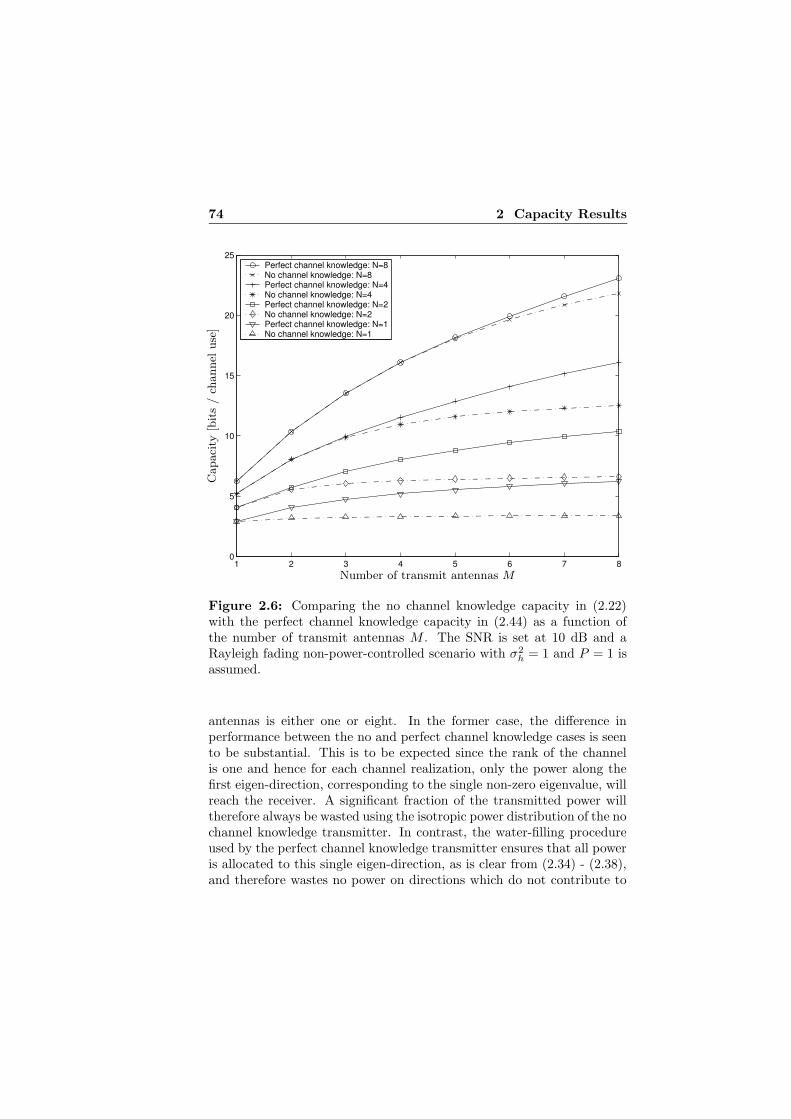
74 2 Capacity Results
1 2 3 4 5 6 7 80
5
10
15
20
25Perfect channel knowledge: N=8No channel knowledge: N=8Perfect channel knowledge: N=4No channel knowledge: N=4Perfect channel knowledge: N=2No channel knowledge: N=2Perfect channel knowledge: N=1No channel knowledge: N=1
PSfrag replacements
Number of transmit antennas M
Capaci
ty[b
its
/ch
annel
use
]
Figure 2.6: Comparing the no channel knowledge capacity in (2.22)with the perfect channel knowledge capacity in (2.44) as a function ofthe number of transmit antennas M . The SNR is set at 10 dB and aRayleigh fading non-power-controlled scenario with σ2
h = 1 and P = 1 isassumed.
antennas is either one or eight. In the former case, the difference inperformance between the no and perfect channel knowledge cases is seento be substantial. This is to be expected since the rank of the channelis one and hence for each channel realization, only the power along thefirst eigen-direction, corresponding to the single non-zero eigenvalue, willreach the receiver. A significant fraction of the transmitted power willtherefore always be wasted using the isotropic power distribution of the nochannel knowledge transmitter. In contrast, the water-filling procedureused by the perfect channel knowledge transmitter ensures that all poweris allocated to this single eigen-direction, as is clear from (2.34) - (2.38),and therefore wastes no power on directions which do not contribute to

2.7 Numerical Examples 75
the received signal.The eight receive antenna curves demonstrate the high data rates
offered by a MIMO structure with an equal number of transmit andreceive antennas. Typically, all eigen-directions now contribute, moreor less, to the received signal. It is therefore not surprising that thenon-informed transmitter with its spatially isotropic power distributionperforms almost as well as the water-filling transmitter. The performancegap is no longer constant and is even seen to vanish at high SNR values.Such a decreasing performance gap is reasonable in view of the water-filling power distribution which becomes more uniform, or more spatiallyisotropic, as the SNR is increased. The utility of channel knowledgeis hence larger when the SNR is low than when it is high. This is arather general phenomenon that will also be observed in later chapters inconnection with performance evaluation of codes designed to take channelknowledge into account.
The impact of different antenna configurations on the performanceis further illustrated in Figure 2.6. The SNR is now fixed at 10 dBand the number of transmit and receive antennas is varied. Again, it isseen that the gains due to channel knowledge are more pronounced whenthe difference between the number of transmit and receive antennas islarge. By connecting the data points corresponding to an equal numberof antennas at both sides, it is also possible to discern the linear increasein capacity with respect to M = N that is typical of MIMO systems andwhich was reported in e.g. [FG98].
2.7.2 Quantized Channel Information
As previously mentioned, quantized channel information obtained fromthe receiver via a feedback link is frequently encountered in practice. Ob-viously, such partial channel knowledge is better than none at all while,on the other hand, the performance cannot be expected to be as goodas when the channel is known perfectly. This tradeoff is to some extentinvestigated below for the memoryless deterministic quantized feedbackscenario described in Section 2.6.2, assuming a scenario with power con-trol. Hence, each channel realization is independently quantized into aQ-valued integer i(n) by a deterministic feedback encoder function ε(·).The encoder output constitutes the side information, i.e., ζ(n) = i(n).To facilitate an easy computation of the capacity, the study is limited toone receive antenna and quantization schemes that exhibit a high degreeof symmetry, permitting the use of the theory of symmetric feedback. In

76 2 Capacity Results
practice, the assumption of one receive antenna is not as restrictive as itmay first seem since the terminals in many wireless systems are typicallynot equipped with more than one antenna. The study therefore coversthe important case of communication in the downlink from for examplea base station with several antennas to a single antenna terminal. Inparticular, the setup is closely related to the one in the closed-loop modeof the WCDMA system [3GP02b].
0 5 10 15 20 25 300
2
4
6
8
10
12Perfect channel knowledgePhase and amplitude quantization: b=4Phase quantization: b=2Phase quantization: b=1No channel knowledge
PSfrag replacements
Capaci
ty[b
its
/ch
annel
use
]
SNR [db]
Figure 2.7: Capacity as a function of SNR for different levels of quanti-zation. A Rayleigh fading power-controlled scenario with M = 2 transmitantennas, N = 1 receive antenna, σ2
h = 1 and P = 1 is assumed.
Consider a system with M = 2 transmit antennas and N = 1receive antenna system that employs uniform phase quantization ofH(n)/H11(n) = H12(n)/H11(n) as defined by (2.60) and (2.61). Thefeedback scenario is symmetric and the capacity is therefore given by(2.63). In Figure 2.7, numerical results on the capacity as a function ofthe SNR are depicted for no channel knowledge, b = 1 and b = 2 bit quan-
2.8 Conclusions 77
tization. In addition, the expression for the power constraint in (2.52)was used to provide numerical values on the capacity when the chan-nel is known perfectly. One bit quantization is seen to give a significantimprovement over the no channel knowledge case. Adding another bitgives only a modest improvement which however takes the performancequite close to the limiting perfect channel knowledge case. To come evencloser to this limit, also the amplitude needs to be quantized. Considertherefore a second type of quantization scheme in which the encoder isstill given by (2.60) but with the encoder codebook
εk =
[
1 0.8ejπk/4]T
, k = 0, · · · , 7[
1 1.6ejπ(k−8)/4]T
, k = 8, · · · , 15 ,
which means that the relative phase is quantized using three bits while afourth bit is used to quantize the relative amplitude. It is easily verifiedthat the feedback is now symmetric with respect to Sk7
k=0 or Sk15k=8,
respectively. Computing the capacity is hence feasible since (2.58) showsthat only two different matrices need to be optimized. The resultingb = 4 curve in Figure 2.7 is seen to almost coincide with the performanceof the perfect channel knowledge transmitter.
Finally, phase-only quantization as described above is further investi-gated in Figure 2.8 illustrating how the performance is affected by increas-ing the number of transmit antennas M while keeping the quantizationlevel at b = b/(M − 1) = 2 bits per complex dimension. Again, the noand perfect knowledge cases serve as benchmarks. Increasing M abovetwo basically does not improve the performance when there is no channelinformation. On the other hand, when using the phase quantization, thecapacity increases substantially with the number of transmit antennas.This agrees well with the previous results displayed in Figure 2.6. Weconclude that it is possible to come quite close to the limiting perfectchannel knowledge curves using only phase quantization.
2.8 Conclusions
This work considered a MIMO wireless communication link in which thetransmitter has access to possibly imperfect channel side information. Aformula for the channel capacity was presented and subsequently ana-lyzed for a number of different cases.

78 2 Capacity Results
0 5 10 15 20 25 300
2
4
6
8
10
12Perfect channel knowledge: M=4Phase quantization: M=4, b=6No channel knowledge: M=4Perfect channel knowledge: M=3Phase quantization: M=3, b=4No channel knowledge: M=3Perfect channel knowledge: M=2Phase quantization: M=2, b=2No channel knowledge: M=2
PSfrag replacements
Capaci
ty[b
its
/ch
annel
use
]
SNR [db]
Figure 2.8: Capacity as a function of SNR for different levels of phasequantization and number of transmit antennas. A Rayleigh fading power-controlled scenario with N = 1 receive antenna, σ2
h = 1 and P = 1 isassumed.
One important result is that separate space-time coding and transmitweighting is an optimal transmission structure. In the case of a systemwith two transmit antennas and one receive antenna, it was shown thatsuch a structure may utilize the well-known Alamouti space-time codewithout loss of optimality.
Although the focus was on a power-controlled scenario, it was alsopointed out that the presented capacity expression is easy to modify toencompass also the case of a power constraint preventing the use of powercontrol. An interesting side effect of this is that previously used averagecapacity or expected mutual information based performance measuresindeed correspond to true channel capacities.
Methods for evaluating the often numerically challenging capacity ex-

2.8 Conclusions 79
pression were developed. In particular, a theory concerned with symmet-rical properties of typical channel feedback schemes was introduced andused for simplifying numerical computation of the capacity. Numericalresults on the channel capacity demonstrated the importance of exploit-ing channel side information.

80 2 Capacity Results
Appendix 2.A Proving Optimality of Block
Diagonal Structure
In this appendix, it is proved that Z(ζ) in the capacity formula (2.13)may be taken to be block diagonal without loss of optimality.
The proof proceeds as follows. Partition Z(ζ) into L2 blocks accord-ing to
Z(ζ) =
Z11(ζ) · · · Z1L(ζ)...
...ZL1(ζ) · · · ZLL(ζ)
,
where each block is represented by the M ×M sub-matrix Zkl(ζ). Basedon the above partition of Z(ζ), it is possible to write
(IL ⊗ R−1/2ee H)Z(ζ)(IL ⊗ H∗(R−1/2
ee )∗)
=
R−1/2ee HZ11(ζ)H∗(R−1/2
ee )∗ · · · R−1/2ee HZ1L(ζ)H∗(R−1/2
ee )∗
......
R−1/2ee HZL1(ζ)H∗(R−1/2
ee )∗ · · · R−1/2ee HZLL(ζ)H∗(R−1/2
ee )∗
.
Consider the determinant in (2.13) and use the relation (C.5) in Ap-pendix C and Fisher’s inequality [HJ96, p. 478] to obtain the upper bound
det(ILN + (IL ⊗ R−1ee )(IL ⊗ H)Z(ζ)(IL ⊗ H∗))
= det(ILN + (IL ⊗ R−1/2ee H)Z(ζ)(IL ⊗ H∗(R−1/2
ee )∗))
≤L∏
k=1
det(IN + R−1/2ee HZkk(ζ)H∗(R−1/2
ee )∗) , (2.64)
which holds with equality if all sub-matrices Zkl(ζ) that are not on themain diagonal are zero. Utilize (2.64) and the fact that log2 det(·) is aconcave function to write
E[det(ILN + (IL ⊗ R−1ee )(IL ⊗ H)Z(ζ)(IL ⊗ H∗))]
≤ E[ L∑
k=1
log2 det(IN + R−1/2ee HZkk(ζ)H∗(R−1/2
ee )∗)]
≤ LE[
log2 det(IN + R−1/2ee H
∑Lk=1 Zkk(ζ)
LH∗(R−1/2
ee )∗)]
, (2.65)

2.B Proving Optimality of Diagonal Structure 81
where last step follows from the definition of a concave function. Thesecond inequality holds with equality if the Zkk(ζ)’s are all equal. Fur-thermore, note that the power constraint in (2.13) can be written as
E[tr(Z(ζ))] = E[
tr( L∑
k=1
Zkk(ζ))]
= Pbm . (2.66)
From (2.65) and (2.66) it is now seen that an upper bound on the capacityin (2.13) is given by
C ≤ maxZkk(·)
Zkk(·)=Zkk(·)∗0, ∀k
E[
tr(∑L
k=1 Zkk(ζ))]
=Pbm
LE[log2 det(IN + R−1/2ee H
∑
k Zkk(ζ)
LH∗(R−1/2
ee )∗)]
= maxZ(·)
Z(·)=Z(·)∗0
L E[tr(Z(ζ))]=Pbm
LE[log2 det(IN + R−1/2ee HZ(ζ)H∗(R−1/2
ee )∗)] ,
(2.67)
where (2.67) follows from reformulating the optimization problem interms of the parametrization Z(ζ) ,
∑
k Zkk(ζ)/L. However, the aboveinequality holds with equality since (2.67) may be obtained directly fromthe capacity formula in (2.13) if Z(ζ) is constrained as Z(ζ) = IL⊗Z(ζ).Hence, (2.67) gives the capacity and we have shown that Z(ζ) may betaken to be block diagonal without loss of optimality, as asserted.
Appendix 2.B Proving Optimality of Diag-
onal Structure
In this appendix, the optimality of the diagonal structure in (2.27) willbe proved. Although somewhat shortened, the development proceedsin a similar manner as for the proof concerned with the block diagonalstructure in Appendix 2.A.
Let [A]kl denote the element on the kth row and lth column of the ma-trix A and use this to define Zkk(H) , [Z(H)]kk. Applying Hadamard’sinequality [HJ96, p. 477] to the determinant gives
det(IN + Λ(H)Z(H)) ≤r∏
k=1
(1 + [Λ(H)Z(H)]kk)

82 2 Capacity Results
=r∏
k=1
(1 + [Λ(H)]kk[Z(H)]kk)
=r∏
k=1
(1 + λk(H)Zkk(H)) , (2.68)
with obvious notation. The above upper bound is attained if Z(H) isdiagonal. Furthermore, note that
E[tr(Z(H))] =
M∑
k=1
E[Zkk(H)] = P ,
which means that also the power constraint can be written in terms of thediagonal elements of Z(H). Since (2.68) is attained if Z(H) is diagonaland both the upper bound and the power constraint can be written interms of the corresponding diagonal elements, Z(H) may be assumed tobe diagonal without loss of optimality. This concludes the proof.
Appendix 2.C Power Constraint in Closed-
Form
In this appendix, we prove that the power constraint in (2.38) can, as-suming N = 1 receive antenna and spatially IID Rayleigh fading as inSection 2.6.1, be written in closed-form to arrive at (2.52).
Note first that x , 2‖H‖2/σ2h is a chi-squared random variable with
2M degrees of freedom. Hence, its PDF is given by [Kay98, p. 24]
px(x) =
xM−1 exp(−x/2)
2M (M−1)!, x ≥ 0
0, x < 0 .
Let α , σ2/σ2h and evaluate the expectation in the power constraint as
EH [max1/µ − σ2/‖H‖2, 0] = Ex[max1/µ − 2σ2/(σ2hx), 0]
=
∫
max1/µ − 2α/x, 0px(x) dx
=
∫ ∞
2αµ
(1/µ − 2α/x) px(x) dx
=1
µ
∫ ∞
2αµ
px(x) dx − 2α
∫ ∞
2αµ
px(x)/x dx .
2.D Symmetric Feedback 83
Since∫
xneax dx =(−1)n exp(ax)n!
an+1
n∑
k=0
(ax)k(−1)k
k!
it follows that
∫ ∞
2αµ
px(x) dx =1
2M (M − 1)!
∫ ∞
2αµ
xM−1 exp(−x/2) dx
=
[
(−1)M−1 exp(−x/2)(M − 1)!
2M (M − 1)!(−1/2)M
M−1∑
k=0
(−x/2)k(−1)k
k!
]∞
2αµ
= exp(−αµ)M−1∑
k=0
(αµ)k
k!
and
∫ ∞
2αµ
px(x)/x dx =1
2M (M − 1)!
∫ ∞
2αµ
xM−2 exp(−x/2) dx
=
[
(−1)M−2 exp(−x/2)(M − 2)!
2M (M − 1)!(−1/2)M−1
M−2∑
k=0
(−x/2)k(−1)k
k!
]∞
2αµ
=exp(−αµ)
2(M − 1)
M−2∑
k=0
(αµ)k
k!.
Hence, the desired expression in (2.52) follows as
EH [max1/µ − σ2/‖H‖2, 0]
=exp(−αµ)
µ
M−1∑
k=0
(αµ)k
k!− α
exp(−αµ)
M − 1
M−2∑
k=0
(αµ)k
k!.
Appendix 2.D Symmetric Feedback
In this appendix, we derive how the symmetric feedback conditions inSection 2.6.3 affect the capacity formula. Hence, both the first and secondcondition are tacitly assumed to be satisfied for the remainder of thissection.
84 2 Capacity Results
2.D.1 Encoder Probabilities and Conditional Expec-tation
The expressions in (2.56), (2.57) for the feedback encoder probabilitiesand the conditional expectation, respectively, will be proved below. Theproof relies on symmetries induced by the symmetric feedback conditions.To start with, note that
pκ(q)(0) = Pr[H ∈ Sκ(q)(0)]
=
∫
H∈Sκ(q)(0)
pH(H) dH ,
where the notation “dH” means that the integration is to be carried outwith respect to the 2MN real-valued parameters of H. Now utilize thefirst condition and make a change of variables to obtain
pκ(q)(0) =
∫
HQ(q)k
∈Sκ(q)(k)
pH(H) dH
=
∫
H∈Sκ(q)(k)
pH
(H(Q
(q)k )∗
)dH ,
where the second equality follows from the fact that the determinantof the Jacobian of a unitary linear transformation is one. The secondcondition finally gives
pκ(q)(0) =
∫
H∈Sκ(q)(k)
pH(H) dH
= Pr[H ∈ Sκ(q)(k)]
= pκ(q)(k) ,
which shows that all encoder output probabilities belonging to the qthsubset are equal, as claimed in (2.56).
Let pH|i(H|i = κ(q)(k)) denote the PDF of H conditioned on the
event that i = κ(q)(k), which corresponds to H ∈ Sκ(q)(k). To prove theresult on the conditional expectation, first note that
pH|i(H|i = κ(q)(k)) =
pH(H)p
κ(q)(k)
, H ∈ Sκ(q)(k)
0, otherwise

2.D Symmetric Feedback 85
and hence, because of the unitary invariance pH(HU) = pH(H), thefirst condition and pκ(q)(0) = pκ(q)(k),
pH|i(H|i = κ(q)(0)) =
pH(HQ(q)k
)
pκ(q)(0)
, H ∈ Sκ(q)(0)
0, otherwise
=
pH(HQ(q)k
)
pκ(q)(k)
, HQ(q)k ∈ Sκ(q)(k)
0, otherwise
= pH|i(HQ(q)k |i = κ(q)(k)) .
From this the desired relation in (2.57) follows as
E[log2 det(IN + R−1ee HXH∗)|i = κ(q)(k)]
=
∫
log2 det(IN + R−1ee HXH∗)pH|i(H|i = κ(q)(k)) dH
=
∫
log2 det(IN+R−1ee HQ
(q)k X(Q
(q)k )∗H
∗)pH|i(HQ
(q)k |i = κ(q)(k)) dH
=
∫
log2 det(IN + R−1ee HQ
(q)k X(Q
(q)k )∗H
∗)pH|i(H|i = κ(q)(0)) dH
= E[log2 det(IN + R−1ee HQ
(q)k X(Q
(q)k )∗H∗)|i = κ(q)(0)] .
2.D.2 Simplifying the Optimization Problem
This section presents a proof that the capacity formula in (2.53) simplifies
to (2.58). By grouping terms that correspond to the same subset S (q)s
together and utilizing (2.56) and (2.57), the power constraint can berewritten as
Q−1∑
k=0
pk tr(Zk) =
Q′−1∑
q=0
∑
k∈I(q)s
pk tr(Zk)
=
Q′−1∑
q=0
|I(q)s |−1∑
k=0
pκ(q)(k) tr(Zκ(q)(k))
=
Q′−1∑
q=0
pκ(q)(0)
|I(q)s |−1∑
k=0
tr(Zκ(q)(k)) = P
86 2 Capacity Results
and the criterion function as
Q−1∑
k=0
pk E[log2 det(IN + R−1ee HZkH∗)|H ∈ Sk]
=
Q′−1∑
q=0
∑
k∈I(q)s
pk E[log2 det(IN + R−1ee HZkH∗)|i = k]
=
Q′−1∑
q=0
|I(q)s |−1∑
k=0
pκ(q)(k) E[log2 det(IN + R−1ee HZκ(q)(k)H
∗)|i = κ(q)(k)]
=
Q′−1∑
q=0
pκ(q)(0)
|I(q)s |−1∑
k=0
f (q)(Q
(q)k Zκ(q)(k)(Q
(q)k )∗
),
where
f (q)(X) , E[log2 det(IN + R−1ee HXH∗)|i = κ(q)(0)] .
Now re-parameterize the problem using Z(q)
k , Q(q)k Zκ(q)(k)(Q
(q)k )∗.
Since Q(q)k is unitary, tr(Zκ(q)(k)) = tr((Q
(q)k )∗Z
(q)
k Q(q)k ) = tr(Z
(q)
k ) andthe power constraint becomes
Q′−1∑
q=0
pκ(q)(0)
|I(q)s |−1∑
k=0
tr(Z(q)
k ) = P .
The resulting capacity is hence
C = maxZ
(q)k
Z(q)k =(Z
(q)k )∗0, ∀k,q
∑Q′−1q=0 p
κ(q)(0)
∑|I(q)s |−1
k=0 tr(Z(q)k )=P
Q′−1∑
q=0
pκ(q)(0)
|I(q)s |−1∑
k=0
f (q)(Z
(q)
k
). (2.69)
Note that f (q)(X) is a concave function of the set of positive semi definitematrices. Hence, we have
|I(q)s |−1∑
k=0
f (q)(Z
(q)
k
)≤ |I(q)
s |f (q)
(∑|I(q)s |−1
k=0 Z(q)
k
|I(q)s |
)
,

2.D Symmetric Feedback 87
which holds with equality if the Z(q)
k ’s are equal for all k ∈ I(q)s . This
means that an upper bound on the capacity in (2.69) is given by
C ≤ maxZ
(q)k
Z(q)k =(Z
(q)k )∗0, ∀k,q
∑Q′−1q=0 p
κ(q)(0)
∑|I(q)s |−1
k=0 tr(Z(q)k )=P
Q′−1∑
q=0
pκ(q)(0)|I(q)s |f (q)
(∑|I(q)s |−1
k=0 Z(q)
k
|I(q)s |
)
= maxZ
(q)Q′−1
q=0
Z(q)
=(Z(q)
)∗0, ∀q∑Q′−1
q=0 pκ(q)(0)
|I(q)s | tr(Z
(q))=P
Q′−1∑
q=0
pκ(q)(0)|I(q)s |f (q)
(Z
(q)), (2.70)
where the equality is due to a straightforward re-parametrization based
on Z(q)
,∑|I(q)
s |−1k=0 Z
(q)
k /|I(q)s |. Clearly, if we for all k ∈ I(q)
s constrain
Z(q)
k in the capacity formula in (2.69) to be equal to Z(q)
, the result is(2.70). In other words, the upper bound is attainable and the capacitycan therefore be computed according to
C = maxZ
(q)Q′−1
q=0
Z(q)
=(Z(q)
)∗0, ∀q∑Q′−1
q=0 pκ(q)(0)
|I(q)s | tr(Z
(q))=P
Q′−1∑
q=0
pκ(q)(0)|I(q)s |f (q)
(Z
(q)). (2.71)
An optimal solution of the original problem in (2.69) is given by Z(q)
k =
Z(q)
, ∀k, where Z(q)
is the maximizing argument of (2.71). This con-cludes the proof.
2.D.3 Proving Symmetry of Feedback in the Exam-ple Scenario
In this appendix it is proved that the uniform phase quantization schemein (2.60), under the assumptions of one receive antenna and spatiallyIID Rayleigh fading channel coefficients, results in a symmetric feedbackscenario. In other words, we will show that the feedback is symmetricwith respect to all encoder regions. This will be accomplished by showing
that the two feedback conditions are satisfied for S (0)s = SkQ−1
k=0 , Q(0)k =

88 2 Capacity Results
Qk, with Qk defined as in (2.62) and the renumbering function κ(0)(k) =k.
Since the channel coefficients are zero-mean IID and each channelcoefficient is complex Gaussian distributed with variance σ2
h, the PDFpH(H) of the channel is given by [Kay93, p. 507]
pH(H) =exp
(−∑M
k=1 |H1k|2/σ2h
)
πMσ2Mh
=exp(−HH∗/σ2
h)
πMσ2Mh
.
Note that (HU)(HU)∗ = HUU∗H∗ = HH∗ for an arbitrary unitarymatrix U . Hence, pH(HU) = pH(H) and the second feedback conditionis seen to be satisfied.
To see that also the first feedback condition is satisfied, assume thatH ∈ Sκ(q)(0) = S0. That is, expressed using the encoder function in(2.60), it holds that
ε(H) = arg minl
‖HT/H11 − Qlε0‖2 = 0 , (2.72)
where Qlε0 = εl. The output of the encoder with HQ(0)k = HQk as
input, is then
ε(HQk) = arg minl
‖QTk HT/H11 − Qlε0‖2
= arg minl
‖QkHT/H11 − Qlε0‖2
= arg minl
‖Qk(HT/H11 − Q∗kQlε0)‖2
= arg minl
‖HT/H11 − Q∗kQlε0‖2 ,
where the last inequality is due to the fact that the Euclidean vector normis invariant to a unitary linear transformation. Because of the uniformphase quantization, it is realized that Q∗
kQl ∈ QmQ−1m=0. Hence, Q∗
kQl
represents an arbitrary Qm and, from Q∗kQk = IM = Q0 in conjunction
with (2.72), it follows that
ε(HQk) = arg minl
‖HT/H11 − Q∗kQlε0‖2 = k .
This shows that HQk = HQ(0)k ∈ Sk = Sκ(q)(k) and consequently
that H ∈ Sκ(q)(0) ⇒ HQ(0)k ∈ Sκ(q)(k). To prove the converse, assume
HQ(0)k = HQk ∈ Sκ(q)(k) = Sk, i.e.,
ε(HQk) = arg minl
‖QTk HT/H11 − Qlε0‖2 = k . (2.73)

2.D Symmetric Feedback 89
The encoder output with H as input is then
ε(H) = arg minl
‖HT/H11 − Qlε0‖2
= arg minl
‖Qk(HT/H11 − Qlε0)‖2
= arg minl
‖QTk HT/H11 − QkQlε0)‖2 = 0 ,
where the last equality follows from QkQl ∈ QmQ−1m=0 and QkQ0 = Qk
in conjunction with (2.73). Consequently, H ∈ S0 = Sκ(q)(0) and the
converse is proved. Thus, H ∈ Sκ(q)(0) ⇔ HQ(0)k ∈ Sκ(q)(k), meaning
that also the first feedback condition is satisfied.


Chapter 3
System Description andPreliminaries
The remainder of the thesis is concerned with code and transmissionscheme design for transmitters with possibly imperfect channel side in-formation. The design methods are to a large extent developed based onthe same system model. The present chapter describes the parts of thesystem model that all the design methods have in common. This genericsystem model will in later chapters be supplemented with additional as-sumptions for the respective case under study.
In the following, essentially a special case of the flat block fading sce-nario in Section 2.3.2 is considered. A data model is presented and threedifferent classes of channel side information dependent space-time blockcodes are described for later reference. The code classes, mentioned inorder of increasingly restrictive structure, are unstructured codes, lineardispersive codes and weighted OSTBC. While the first two code typesare simple extensions of structures previously known in the literature,weighted OSTBC was originally proposed in the works that form thisthesis and hence represents a new code/transmission structure.
3.1 A Generic System Model
Consider a MIMO wireless communication system in a flat block fadingscenario with channel side information at the transmitter under assump-tions that essentially correspond to a special case of the flat block fading
92 3 System Description and Preliminaries
scenario in Section 2.3.2. Hence, both the channel and the side infor-mation is constant during a block of L samples but may vary from oneblock to another in a statistically stationary fashion. However, in con-trast to the previous scenario, the channel coding is now assumed to beperformed independently for each block. More specifically, the length ofthe codewords in the channel code is equal to the block length L andeach transmitted codeword experiences only one channel realization.
A typical benefit of such type of channel coding is that the processingdelay incurred by the coding scheme is relatively short, since the delay ison the same order of magnitude as the block length L. This suits delaysensitive applications such as voice traffic or video conferencing. On theother hand, a drawback is that the temporal variations of the channelare not exploited for achieving time diversity. If needed however, timediversity can be achieved by interleaving and employing an outer code,at the expense of increased processing delay.
Because the channel coding is performed independently for each block,we may restrict our attention to a single arbitrary block, without lossof generality. In the following, the time-interval n = 0, 1, · · · , L − 1 istherefore considered and the block index is dropped.
A symbol sampled complex baseband equivalent model of the sys-tem is depicted in Figure 3.1. At the transmitter, a space-time encodermaps bits, representing the message to be transmitted, into a sequence ofcodeword matrices. The result is a set of parallel and generally differentchannel symbol streams. Each symbol stream corresponds to the signalfor a particular transmit antenna. Side information ζ about the channelis assumed to be available and utilized for adapting the transmission tothe channel characteristics. The space-time encoder has access to a setC(ζ) of codes. Out of this set, the side information is utilized for deter-mining the channel code C currently in use as C = C(ζ). At the receiver,the information carrying signals are first decoded into codewords and theresult is then mapped back into bits, corresponding to an estimate of thetransmitted message. As before, the decoding relies on the assumptionthat both the channel and the side information is known perfectly.
Recall that there are M transmit and N receive antennas. Let H,with complex-valued elements Hkl, be an M ×N matrix used for rep-resenting the MIMO channel1 during the block under consideration as
1Compared with the system model used for the information theoretic investigations,H is now the complex conjugate of the previous MIMO channel matrix. Hence, eachcolumn of H represents the MISO channel between the transmitter’s antenna arrayand the corresponding receive antenna. This will turn out to be convenient.

3.1 A Generic System Model 93
PSfrag replacements
......
Space-Time
EncoderReceiver
H⇔h=vec(H)︷ ︸︸ ︷
C(ζ)
C = C(ζ)
ζ
M N
c(n) x(n)
Figure 3.1: The generic system model.
H∗. Consequently, the SISO channel coefficient between the kth trans-mit antenna and the lth receive antenna is H∗
kl. Furthermore, let theMIMO channel be alternatively represented by its vectorized counterparth , vec(H), with elements hk. Assumptions determining the exactnature of the channel fading will be introduced in later chapters.
The received signals at sample index n ∈ 0, · · · , L− 1 are collectedin a vector x(n), that similarly to (2.12), can be written as
x(n) = H∗c(n) + e(n) ,
where the potentially complex-valued symbols, transmitted from the Mantennas at time instant n, are represented by
c(n) ,[c1(n) c2(n) · · · cM (n)
]T.
The noise term e(n) is assumed to be generated from a zero-mean tempo-rally white complex Gaussian random process with the spatial covariancematrix Ree , E[e(n)e(n)∗] = σ2IN , where σ2 denotes the variance ofthe individual elements in e(n). Thus, the noise is spatially white. Bygrouping the L consecutive vectors x(n) into a matrix X, the receivedblock of vectors can be written as
X = H∗C + E ,
where E contains the noise vectors and
C ,[c(0) c(1) · · · c(L − 1)
]
corresponds to the codeword output by the space-time encoder. Thetransmitted codeword C belongs to the currently used code C = C(ζ) ,

94 3 System Description and Preliminaries
C(ζ)k K
k=1, where K is the number of codewords and C(ζ)k represents the
kth codeword in C(ζ). Note that each codeword is a function of the sideinformation. Hence, the number of codes in the set C(ζ) is possiblyuncountable when ζ is non-discrete.
The data to be transmitted is modeled as an IID sequence of infor-mation bits where both bit-values are equally probable. Since the lengthof the codewords is L, the coding results in a code rate of log2(K)/Linformation bits per channel use. The choice of L and K allows an ap-propriate tradeoff between data rate and time redundancy. Conditionedon the use of a certain code C(ζ), it is assumed that the transmission issuch that all the codewords are equally probable and that the averageenergy/power per information bit is P . In other words, the output poweris limited by
E[‖C‖2F|ζ]
log2(K)= P , (3.1)
which corresponds to a scenario without power control since the averageoutput power does not depend on ζ.
The receiver is assumed to recover the transmitted codewords bymeans of maximum likelihood (ML) decoding. Due to the fact that boththe channel and the side information are known, this amounts to decodingthe codewords according to
C = arg minC∈C(ζ)
‖X − H∗C‖2F , (3.2)
where C denotes the codeword chosen by the receiver. An estimate ofthe part of the transmitted message corresponding to a block is obtainedby mapping the detected codeword into its equivalent bit representation.
3.2 Code Structures
The presence of noise means that the receiver will not always come tothe correct decisions. Hopefully, the probability that the receiver makesan error is sufficiently small for the communication to still be meaning-ful. Channel codes are typically designed with the goal of minimizing theerror probability. But low error probability is not the only criterion toconsider. Also important is that the codes can be decoded in a computa-tionally efficient manner. In the worst case, the receiver has to performan exhaustive search over all the K different codewords like indicated in
3.2 Code Structures 95
(3.2). The previously mentioned capacity achieving codes drawn from aGaussian distribution suffer from such a problem.
To avoid high decoding complexity, it is necessary to introduce struc-ture in the code. Many different code types exist in the literature. Cyclic,convolutional and trellis codes [Pro95] are just a few examples of codetypes that all have in common that additional constraints on the code-words have been imposed in order to lower the decoding complexity.There is however a tradeoff between performance and structure sincestructure generally limits the degrees of freedom in the code design. Com-pletely unstructured codes obviously give the best performance, if de-signed appropriately, but they result in high decoding complexity. Highlystructured codes, on the other hand, may be easy to decode but may alsoperform considerably worse than their unstructured counterparts.
In later chapters of this thesis, the performance versus structure trade-off will to some extent be investigated by designing codes based on threedifferent structures. The code structures under study are unstructuredand linear dispersive space-time block codes as well as weighted OSTBC.The codes have here been mentioned in order of increasingly restrictivestructure and are all examples of channel side information dependentcodes. That is, they are functions of the channel side information vectorζ. As previously mentioned, the unstructured and linear dispersive codesare simple generalizations of previously known code types aimed for theno channel knowledge case while weighted OSTBC is a new transmis-sion structure proposed herein. Further details are given in the sectionsbelow.
3.2.1 Unstructured Space-Time Block Codes
For unstructured space-time block codes, all the elements in all the code-word matrices can be chosen arbitrarily from the complex number fieldC, subject only to the power constraint. In other words, the search for
good codes is over codewords such that C(ζ)k ∈ Ck , C
M×L, for all k andζ. Here, Ck represents the codeword alphabet for the kth codeword. Asalready pointed out, unstructured codes have potentially the best per-formance but result in high decoding complexity since they require anexhaustive search as in (3.2).
For later reference, note that the power constraint in (3.1) can be

96 3 System Description and Preliminaries
written in terms of the codewords as
E[‖C‖2F|ζ] =
1
K
K∑
k=1
‖C(ζ)k ‖2
F = log2(K)P , (3.3)
due to the previously mentioned assumption of equally probable code-words conditioned on ζ.
3.2.2 Linear Dispersive Space-Time Block Codes
When linear dispersive space-time block codes are used, the data to betransmitted corresponding to one codeword is first mapped into symbolssm, m = 1, 2, · · · , Ld, each taken from some signal constellation alphabetA. The transmitted codeword is thereafter formed as a linear combina-tion of the information bearing symbols according to
C =
Ld∑
m=1
Bmsm , (3.4)
where Bm , B(ζ)m represents an arbitrary complex-valued M ×L matrix
used to weigh the mth symbol. Assume without loss of generality2 thatthe signal constellation alphabet A and hence also the symbols sm, arereal-valued. The symbols depend only on the data to be transmittedwhile the weighting matrices may vary with the channel side informationζ. Thus, the transmission is adapted to the available channel knowledgeby letting the side information determine the current set B , BmLd
m=1
of weighting matrices as B = B(ζ) , B(ζ)m Ld
m=1. This is illustrated inFigure 3.2 which represents a more specialized form of the setup in thegeneric system model.
By choosing the weights appropriately, the information may be spreadboth spatially and temporally to obtain diversity benefits and codinggain while taking the channel knowledge available at the transmitterinto account. For the case of no channel side information, such lin-ear dispersive structures have previously been described for example in[TJC99, GS00, HH02b].
A major advantage of the above linear structure is that the decod-ing complexity may in some cases be drastically reduced compared with
2Complex-valued symbols may be handled within the present framework by di-viding the symbols into their real and imaginary parts. The codewords can then bewritten on the same form as in (3.4) but with twice as many terms.

3.2 Code Structures 97
PSfrag replacements
...
Linear Dispersive
Space-Time
Encoder
ReceiverH⇔h=vec(H)
︷ ︸︸ ︷
B(ζ)
B = B(ζ)
ζ
M
N
c(n)
x(n)
smLdm=1
Figure 3.2: Transmitter structure using linear dispersive space-timeblock codes. The channel side information determines the current set Bof weighting matrices.
the complexity of an exhaustive search. The reduction in complexity isachieved by the use of efficient decoding methods [VH02, JMO03] whichtypically only incur a minor increase in error probability due to theirsub-optimal nature. These decoding methods are applicable if the signalconstellation A corresponds to a regular lattice, such as when the sym-bols are taken from a pulse or quadrature amplitude modulation (PAMor QAM) constellation. Sphere decoding is one example of a scheme thatis relatively efficient when the number of codewords K is large [VH02].Decoding methods based on optimization techniques for semi definiteproblems are also applicable assuming the symbols belong to a binaryphase shift keying (BPSK) or a four point QAM constellation [JMO03].
In the code design procedures presented in later chapters, the weight-ing matrices will be optimized based on the available side informa-
tion while the constellation alphabet A will be held fixed. Let s(k)m ,
m = 1, 2, · · · , Ld be the particular symbol sequence corresponding to
the kth codeword C(ζ)k . Using linear dispersive codes thus means that
the codewords are constrained as
C(ζ)k ∈ Ck ,
Ld∑
m=1
Bms(k)m : Bm ∈ C
M×L,∀m
,
for all k and ζ.The constellation alphabet A is throughout this thesis assumed to
correspond to a PAM constellation of equidistant real-valued signal pointssuch that E[sm] = 0 and E[s2
m] = 1. It is further assumed that eachsymbol represents an integer number of information bits. It follows that

98 3 System Description and Preliminaries
the symbols are IID since they have been mapped from an IID sequence ofinformation bits. Hence, the power constraint in (3.1) can be formulatedin terms of the weighting matrices as
E[‖C‖2F|ζ] = E[tr(CC∗)|ζ]
= E[
tr( Ld∑
m=1
Ld∑
m′=1
BlB∗m′smsm′
)
|ζ]
=
Ld∑
m=1
Ld∑
m′=1
tr(
B(ζ)m
(B
(ζ)m′
)∗)
E[smsm′ ]
=
Ld∑
m=1
tr(
B(ζ)m
(B(ζ)
m
)∗)
=
Ld∑
m=1
‖B(ζ)m ‖2
F = P log2(K) . (3.5)
3.2.3 Weighted OSTBC
We propose the weighted OSTBC transmission structure as a simple butyet effective way of exploiting channel side information in conjunctionwith space-time coding. In weighted OSTBC, the idea is to use the sideinformation for improving a predetermined OSTB code by means of a lin-ear transformation. This is in line with the previous information theoreticresult in Section 2.3.1 concerning the optimality of separate space-timecoding and transmit weighting. Indeed, weighted OSTBC has alreadybeen briefly described in connection with the information theoretic inves-tigation in Section 2.5, where it was proved that the structure is optimalin a capacity sense if there are two transmit antennas and one receiveantenna.
The transmitted codeword in weighted OSTBC can be written on theform
C = WC , (3.6)
where W , W (ζ) is an M×M ′ transmit weighting matrix which dependson the side information ζ and where C is an M ′ ×L matrix representingthe output of a fixed OSTB encoder. Here, L ≥ M ′, which means thatC has more columns than rows. The OSTB encoder takes the data tobe transmitted corresponding to one codeword and first maps it intosymbols sm, m = 1, 2, · · · , Lo, each taken from some real-valued signal

3.2 Code Structures 99
constellation alphabet A. Again, the symbols are IID and normalized sothat E[s2
m] = 1. Similarly as for the previously described linear dispersiveencoder, the symbols are then linearly combined to form the output as
C =
Lo∑
m=1
Bmsm ,
where the M ′ × L weighting matrices Bm are chosen so that theycorrespond to an OSTB code. The exact conditions under which Bmcorrespond to an OSTB code will be described later in this section. Fornow it suffices to know that they are fixed and hence independent of theside information. Thus, only the transmit weighting W is affected bythe side information, as illustrated in Figure 3.3 where c(n) denotes theoutput of the OSTB encoder.
PSfrag replacements
...OSTB
EncoderW
ReceiverH⇔h=vec(H)
︷ ︸︸ ︷
W (ζ)
W = W (ζ)
ζ
MM ′N
c(n)c(n)
x(n)
smLom=1
Figure 3.3: Transmitter structure in weighted OSTBC. Only the trans-mit weighting W is now affected by the channel side information.
In the weighted OSTBC structure, only W is free to be optimized.Hence, the structure is defined through
C(ζ)k ∈ Ck ,
WCk : W ∈ CM×M ′
, Ck =
Lo∑
m=1
Bms(k)m
, ∀k,∀ζ ,
where s(k)m , m = 1, 2, · · · , Lo denotes the particular symbol sequence cor-
responding to the kth codeword Ck in the OSTB code C , CkKk=1. It
is seen that weighted OSTBC is a special case of the less restrictive lineardispersive code structure.
Before further discussing weighted OSTBC and OSTB codes in gen-eral, it is instructive to consider a specific example illustrating typicalproperties of the transmission structure.

100 3 System Description and Preliminaries
Example 3.2.1 (Weighted OSTBC using the Alamouti code)Consider a scenario with M = 2 transmit antennas and assume thatM ′ = M so that the transmit weighting matrix W is square. Similarlyto (2.47), assume that the OSTB encoder is based on the Alamouticode [Ala98]. Under the assumption that the information symbols arereal-valued, such a choice of code leads to the encoder output
C =
[s1 −s2
s2 s1
]
, (3.7)
which can also be written on the linear dispersive form
C =
[1 00 1
]
s1 +
[0 −11 0
]
s2 . (3.8)
Using this code, the transmitted codeword in weighted OSTBC is givenby
C = WC =[w1 w2
][s1 −s2
s2 s1
]
, (3.9)
where wl denotes the lth column of W . It is seen that the Alamouticode, and hence also the above scheme, has a data rate of one informationsymbol per channel use.
The choice of the transmit weighting W significantly affects the prop-erties of the transmitted signals. Consider first the case when W = I2.The output of the OSTB encoder is then transmitted directly, withoutmodification. As seen from (3.9), the same symbol is transmitted twice atalternating antennas. Switching antennas in this manner serves to pro-tect against fading since if the channels from one of the transmit antennasare poor, there is a good chance that the channels corresponding to theother transmit antenna are better, increasing the likelihood of correctlydecoding the corresponding information symbol.
Note that the transmitted signal block is a unitary matrix, i.e.,CC∗ = CC
∗= (s2
1 + s22)I2. This means that the distribution of energy,
as seen over two sample periods, is isotropic in space. In other words, theenergy is distributed evenly in all directions. As already pointed out inSection 2.3.1, such an energy distribution makes sense if the transmitterdoes not know anything about the channel.
Consider now the case when the second column of W is zero, makingthe rank of the transmit weighting matrix equal to one. It directly followsthat the transmitted codeword
C = WC =[w1s1 −w1s2
]

3.2 Code Structures 101
is also of rank one. Each symbol is now transmitted only once and bothsymbols are weighted by the same vector w1. Thus, classic beamform-ing in the direction of w1 is performed (the minus sign is irrelevant).Clearly, the isotropic energy distribution of the Alamouti code has beenmodified by the transmit weighting so that all energy is allocated to asingle direction. By an appropriate choice of w1 the transmission canbe directed towards the receiver so that the information carrying signalsthere combine coherently. Naturally, this requires knowledge about thechannel at the transmitter.
It should be clear from these two special cases that the transmission,depending on the choice of transmit weighting, may correspond to eitherconventional OSTBC, beamforming or some combination thereof. SinceOSTBC and beamforming are suitable for transmitters with no and per-fect channel knowledge, respectively, weighted OSTBC offers a flexiblestructure that may handle channel side information of varying quality.Thus, the OSTB encoder provides diversity when the quality is low whilethe transmit weighting gives an additional array gain when the quality ishigh.
As long as M ′ = M , the seamless combination of OSTB coding andbeamforming provided by weighted OSTBC holds in the general case aswell and not only in the above example. When M ′ < M beamforming isstill possible but unmodified OSTBC is not, since the transmit weight-ing W has more rows than columns and thus cannot equal the identitymatrix. A spatially isotropic energy distribution is therefore impossible.At best, the energy can be spread evenly over M ′ different directions.However, such a non-square transmit weighting has other merits since itmakes it possible to take an OSTB code designed for a small antennaarray (here small M ′) and map it onto a larger array. This is particularlyimportant in view of the fact that OSTB codes designed for antenna ar-rays with more than two antennas have a much lower maximum symbolrate than the achievable rate when the design is geared towards two an-tennas [TJC99]. The latter issue will be discussed further in the sectionbelow.
Some Properties of OSTB Codes
Probably the most striking characteristic of OSTB codes is the fact thatthe rows (and also the columns if M ′ = L) in each codeword are or-thogonal to each other, or more precisely, form a scaled orthonormal set,

102 3 System Description and Preliminaries
regardless of the symbol sequence. In other words, the weights Bm aresuch that, for arbitrary real-valued constellation alphabets A,
CkC∗k =
Lo∑
m=1
(s(k)
m
)2IM ′ , k = 1, 2, · · · ,K . (3.10)
The very notion of an OSTB code is in fact defined by the orthogonalityproperty in (3.10), together with the linear dispersive structure of thecode.
It is straightforward to show that for (3.10) to hold, the weights Bmmust satisfy the following conditions [TJC99]
BkB∗k = IM ′ , k = 1, 2, · · · , Lo (3.11)
BkB∗l + BlB
∗k = 0M ′×M ′ , 1 ≤ k < l ≤ Lo . (3.12)
Depending on the symbol rate and the value of M ′, such weights, orequivalently OSTB codes, may or may not exist [TJC99]. In particu-lar, OSTB codes with the maximum rate of two real-valued symbols perchannel use (corresponding to a rate of one complex-valued symbol perchannel use) only exist for the case of M ′ = 2. Furthermore, when M ′
lies between three and eight, the symbol rate cannot be higher than one.For all other M ′, the rate must be even lower for the conditions in (3.10)or in (3.11) and (3.12) to hold. It is easily verified that the weightingmatrices in (3.8) satisfy the above conditions.
A direct consequence of the orthogonal property in (3.10) and thelinearity of the code is that
A(Ck, Cl) , (Ck − Cl)(Ck − Cl)∗
=
Lo∑
m=1
(s(k)
m − s(l)m
)2IM ′ , ∀k, l . (3.13)
Hence, also the rows in all pair of codeword differences form a scaledorthonormal set.
The codeword pair quantity in (3.13) plays a fundamental role in thefield of space-time coding since it often appears in expressions for theerror probability. To be specific, assume a spatially uncorrelated flatRayleigh fading scenario. Furthermore, consider the use of an arbitraryfixed space-time code with codewords Ck, i.e., the code does not rely onany channel side information. It can then be shown that the codeword er-ror probability for high SNR values roughly decays as 1/(CG·SNR)Nrmin ,

3.2 Code Structures 103
where CG is the so-called coding gain and where rmin is equal to the min-imum rank of A(Ck,Cl), taken over all codewords pairs [TSC98]. Thevalue of the exponent Nrmin clearly has a large impact on the perfor-mance and is referred to as the (spatial) diversity order of the system.
If Ck = Ck so that unmodified OSTB codewords are transmitted, itfollows from the property in (3.13) that all A(Ck,Cl), with k 6= l, are offull rank. Hence, Nrmin = NM ′ = NM . This shows that OSTB codesprovide a diversity order equal to the product of the number of transmitand receive antennas, which is the maximum diversity order the systemcan offer.
Design methods for conventional space-time codes usually strive toachieve the maximum diversity order while at the same time attempt toincrease the coding gain. One common design method is to maximizethe determinant of A(Ck,Cl) over all codeword pairs [TSC98]. Later onin the thesis, A(Ck,Cl) will be frequently used in performance criteriathat take also the channel knowledge into account.
Weighted OSTBC – ML Decoding and Power Constraint
Recall that weighted OSTBC is a special case of the previously describedlinear dispersive structure. Hence, performance has potentially been sac-rificed by means of a more restrictive structure in order to obtain lowerdecoding complexity. In this case, the decoding complexity is significantlylower thanks to the orthogonality property in (3.10), which makes MLdecoding of OSTBC [TSC98], and hence also weighted OSTBC, very ef-ficient. To see why, consider the ML decoding metric in (3.2) and rewriteit for the problem at hand as
‖X − H∗C(ζ)k ‖2
F = ‖X − H∗W (ζ)Ck‖2F
= tr((X − H∗W (ζ)Ck)(X − H∗W (ζ)Ck)∗)
= tr(XX∗) − tr(XC∗k(W (ζ))∗H + H∗W (ζ)CkX∗)
+ tr(H∗W (ζ)CkC∗k(W (ζ))∗H)
= tr(XX∗) − 2 re(tr(H∗W (ζ)CkX∗))
+ tr(H∗W (ζ)CkC∗k(W (ζ))∗H)
= −2 re
(
tr
(
H∗W (ζ)( Lo∑
m=1
Bms(k)m
)
X∗
))

104 3 System Description and Preliminaries
+ tr(H∗W (ζ)(W (ζ))∗H)
Lo∑
m=1
(s(k)
m
)2+ tr(XX∗)
= tr(XX∗) −Lo∑
m=1
f(Bm, s(k)m ) ,
where re(x) denotes the real part of x and where
f(B, s) , 2 re(tr(X∗H∗W (ζ)B))s − s2‖H∗W (ζ)‖2F .
It is seen that minimizing the ML decoding metric with respect to theset of possible codewords can be accomplished by maximizing the termsin the sum separately. Hence, the symbols may be decoded individuallyas
sm = arg maxs∈A
2 re(tr(X∗H∗W (ζ)Bm))s − s2‖H∗W (ζ)‖2F . (3.14)
Such separate decoding is attractive because the number of comparisonshas now decreased to Lo|A|, compared with |A|Lo = K as in joint de-coding. For signal constellations with many points and/or codes with alarge number of symbols, the difference in complexity can be substantial.
Note that by inserting the expression for X in (3.14) and thereafterutilizing (3.12), it can be shown that ML decoding can be performed inan interference-free manner, i.e., when a certain symbol is decoded, thevalues of the other symbols do not affect the decision in any way. It canalso be shown that the symbol error probabilities are all equal.
In addition to a simpler decoding metric, the orthogonality propertysimplifies the power constraint in (3.1) so that it can be expressed in
terms of the transmit weighting W (ζ) as
E[‖C‖2F|ζ] = E[‖WC‖2
F|ζ]
= tr((W (ζ))∗W (ζ) E[CC∗])
= tr((W (ζ))∗W (ζ))
Lo∑
m=1
E[s2m]
= tr((W (ζ))∗W (ζ))Lo
= Lo‖W (ζ)‖2F = P log2(K) . (3.15)

Chapter 4
Code Design withGaussian SideInformation in Mind
In this chapter, we consider the case when the transmitter has partial,but not perfect, knowledge about the channel and how to design chan-nel side information dependent space-time block codes so that this fact istaken into account. The development is based on the previously describedgeneric system model which here is specialized by in addition assumingthat the channel conditioned on the side information is complex Gaus-sian distributed. The model covers scenarios in which the channel andthe side information are correlated and obey a jointly complex Gaussiandistribution. An important example of such a scenario is when the sideinformation corresponds to delayed channel feedback.
Design procedures for the three code structures are developed. How-ever, the focus is primarily on weighted OSTBC and how to efficientlydetermine the transmit weighting. Toward this end, the optimizationproblem corresponding to the transmit weight design procedure is shownto be convex when the transmit weighting is a square matrix. Thus,standard numerical methods can be used for efficiently obtaining a so-lution. In addition, a particularly efficient solution method is developedfor the special case of independently fading channel coefficients. Theproposed weighted OSTBC transmission scheme combines the benefits ofconventional beamforming with those given by OSTB coding. Simulation

106 4 Code Design with Gaussian Side Information in Mind
results for a narrowband system with multiple transmit antennas and oneor more receive antennas demonstrate significant gains over conventionalmethods in a scenario with non-perfect channel knowledge.
4.1 Introduction
The use of transmit diversity techniques in wireless communication sys-tems has recently received considerable attention [HH78, Wit91, HAN92,Wit93, Mog93, Wee93, SW93, Win94, KF97, Win98, TSC98, GFBK99,TJC99]. By utilizing antenna arrays at both the transmitter as well asthe receiver the limitations of the radio channel may be overcome andthe data rates increased. The high data rates that these MIMO systemsmay offer were demonstrated in [Tel95, FG98]. Therein, calculations ofthe information theoretic capacity assuming a flat Rayleigh fading envi-ronment were presented. This triggered the development of space-timecodes [GFBK99, TSC98, TJC99] that utilize both the spatial and tem-poral dimension to achieve a significant portion of the aforementionedcapacity.
The present work considers the generic system model described inSection 3.1 and investigates how channel side information at the trans-mitter can be utilized in the design of space-time block codes. Accurateestimates are in practice not always possible, particularly in environmentswhere the parameters of the channel are rapidly time-varying. This factis taken into account in the proposed design procedures by modeling thechannel knowledge as non-perfect. As a result, the scheme continues towork well also when the quality of the side information is low.
Early attempts at designing transmission schemes for exploiting thepotential offered by antenna arrays at the transmit side are gener-ally concerned with increasing the diversity order of the system. Ex-amples of such work include techniques for introducing artificial fre-quency/phase offsets [HH78, HAN92, Wee93, KF97] and time offsets[Wit91, Wit93, Mog93, SW93, Win94, Win98] between the transmittedsignals. The latter technique is commonly referred to as delay diversityand is closely related to the layered space-time architecture in [Fos96].A more systematic approach to find appropriate codes was pioneered in[GFK96, GFBK99]. A major contribution in [GFK96, GFBK99] was thedevelopment of a design criterion involving the rank and eigenvalues ofcertain matrices. The design criterion was later generalized to multiplereceive antennas and to other channel models in [TSC98], where the now

4.1 Introduction 107
popular notion of space-time coding was introduced. Examples of trel-lis codes based on the design criterion were also provided. A simple andnovel block code for two transmit antennas that leads to a low-complexityreceiver was developed in [Ala98]. The code is commonly known as theAlamouti code and is a member of the class of OSTB codes that in[TJC99] was extended to up to eight transmit antennas. In the samepaper, it was shown that OSTB codes satisfy the rank constraint of thepreviously mentioned design criterion. Consequently, these codes providethe maximum spatial diversity order the system has to offer.
Common to the space-time coding schemes mentioned above is thatthey do not exploit channel knowledge at the transmitter. Informationabout the channel realization, if it is available, should of course be utilizedin order to maximize the performance. As a simple example consider ascenario with perfect channel state information at both sides of the com-munication link. It is well-known that by appropriate linear processingat the transmitter and the receiver, the system can be transformed intoa set of parallel scalar channels. The available transmit power may thenbe optimally allocated to the individual channels, thereby increasing theperformance relative a system with a transmitter that does not exploitchannel knowledge. An example of combining such an approach withcoding is found in [RC98].
This chapter proposes code design procedures and transmissionschemes that combine the two extremes regarding the degree of chan-nel knowledge. Methods for improving the performance by taking thechannel side information into account are developed for the three codestructures described in Section 3.2. Most of the focus is however onweighted OSTBC and how to reduce the computational requirements ofthe transmit weight design procedure so that real-time use is feasible.An analysis providing insight into the behavior of the resulting transmis-sion scheme is also presented. The side information is modeled using apurely statistical approach in which the channel conditioned on the sideinformation is assumed to obey a complex Gaussian distribution. Animportant special case of this model is when the channel and the sideinformation are correlated and jointly complex Gaussian. Specific atten-tion is devoted to the latter as it offers a reasonable way of modeling thecommon situation of errors introduced by feedback delay.
Previous and related work on the use of non-perfect side informationat the transmitter includes [Wit95, NLTW98, NTC99]. While a simi-lar model for the side information was utilized in [Wit95, NLTW98] fordetermining suitable transmit beamformers in the presence of channel
108 4 Code Design with Gaussian Side Information in Mind
estimation errors, those papers neither considered space-time codes normultiple antennas at the receiver. Another possibility for modeling par-tial channel knowledge is to take on a physical perspective. This is theapproach used in [NTC99] for adapting a predetermined space-time codeto the particular channel. The assumption in that work is that the signalspropagate along a finite number of directions, known at the transmitter,before entering a rich local scattering environment near the receiver.
The present work contributes in several ways. One important contri-bution is the derivation of a new performance criterion that takes channelknowledge at the transmitter into account. Although the derivation isto some extent similar in spirit to the derivation of the design crite-rion in [TSC98], that paper did not treat side information and thereforeutilized certain approximations which prohibit the resulting design cri-terion from exploiting any channel knowledge. Another contribution isthe development and study of techniques for code design. Of particularimportance is our proposed weighted OSTBC structure and the resultinglow-complexity transmission scheme which offers a seamless combinationof OSTB coding and beamforming. Further motivation for weighted OS-TBC is provided by the setup in the WCDMA system, where an OSTBcode is used in one of the transmission modes whereas one of the othermodes uses transmit beamforming [3GP02a, 3GP02b].
The chapter is organized as follows. In Section 4.2, supplements tothe generic system model, including a measure on the quality of the sideinformation, are introduced. Examples of scenarios where the assump-tions are reasonable are also given. A performance criterion is derivedin Section 4.3 and then utilized in Section 4.4 for developing design pro-cedures for the three code types. The remaining part of the chapter isentirely focused on weighted OSTBC. Section 4.5 describes ways to sim-plify the originally proposed transmit weight design procedure, leading toa low-complexity transmission scheme. In Section 4.6, an analyses for anumber of special cases reveal the highly intuitive behavior of the trans-mission scheme. A particularly efficient design algorithm is presented inSection 4.7 for a class of simplified fading scenarios. This algorithm isthen applied in Section 4.8 to an actual example of a simplified fadingscenario. Finally, simulation results are presented in Section 4.9 show-ing significant gains compared to conventional beamforming as well asconventional OSTB coding.

4.2 System Model 109
4.2 System Model
As illustrated in Figure 4.1, a wireless MIMO communication systemwith potentially imperfect channel side information at the transmitter isconsidered. The model of the system was described in Chapter 3 and ishere briefly reviewed before introducing additional assumptions.
PSfrag replacements
......
Space-Time
EncoderReceiver
H⇔h=vec(H)︷ ︸︸ ︷
C(ζ)
C = C(ζ)
ζ
M N
c(n) x(n)
Figure 4.1: System model.
Recall that there are M transmit antennas, N receive antennas andthat L consecutive received signal vectors x(n) = H∗c(n) + e(n), corre-sponding to a fading block, are collected in a matrix
X = H∗C + E ,
where the noise elements in E are zero-mean IID complex Gaussian withvariance σ2, the MIMO channel is represented by the M × N matrixH and where C ∈ C = CkK
k=1 represents the transmitted codeword.Based on the outcome of the side information ζ, the channel code C cur-
rently in use is chosen out of a set C(ζ) of codes as C(ζ) = C (ζ)k K
k=1.The transmitted codewords conditioned on ζ are equally probable andthe power is limited by the constraint
E[‖C‖2F|ζ]
log2(K)= P .
To obtain an estimate C of the transmitted codeword, the receiver makesuse of ML decoding according to
C = arg minC∈C(ζ)
‖X − H∗C‖2F , (4.1)

110 4 Code Design with Gaussian Side Information in Mind
where we recall that H as well as ζ are assumed to be known at thereceiver.
The statistical relation between the side information and the chan-nel was previously not specified. In this chapter, it is generally assumedthat the statistical relation is such that the channel h conditioned onthe side information ζ, denoted h|ζ for short, obeys a complex Gaus-sian distribution with mean vector mh|ζ , E[h|ζ] and covariance matrix
Rhh|ζ , E[(h − mh|ζ)(h − mh|ζ)∗|ζ]. As will be apparent from the de-velopment to follow, both mh|ζ and Rhh|ζ are needed in the code designprocess and hence must be known at the transmitter. However, thesestatistics can usually be computed from some scenario specific parame-ters. Examples of scenarios modeled by the Gaussian assumption will befurther discussed later in the present section.
Note that mh|ζ is the MMSE estimate of h based on ζ [Kay93, p. 533].Since Rhh|ζ is the corresponding conditional error covariance matrix,Rhh|ζ quantifies the remaining uncertainty about the channel h when theside information ζ is known. Hence, the covariance matrix is a measure ofthe quality of the side information. A salient consequence of this measureis that also the distribution of the true channel is considered as part ofthe channel knowledge.
Loosely speaking, high quality side information corresponds to a smallcovariance (measured in a suitable norm) whereas a large covariance cor-responds to side information of low quality. With such a measure, it isclear that “perfect side information” (or “perfect channel knowledge”)corresponds to1 ‖Rhh|ζ‖ → 0, while “no side information” (or “no chan-
nel knowledge”) corresponds to ‖R−1hh|ζ‖ → 0. In both these cases, it is
assumed that ζ is fixed so that Rhh|ζ is a deterministic quantity.However, not all scenarios where the transmitter is without channel
knowledge are covered by the latter definition. This will be more clear ina later section where for illustrative purposes a special case of the systemmodel will be considered, resulting in a need to modify the notion of “nochannel knowledge”.
1Any matrix norm may be used in the definition. The spectral norm used here isonly chosen for the sake of convenience in later expressions.

4.2 System Model 111
4.2.1 Scenarios Modeled by the Gaussian Assump-tion
The Gaussian assumption regarding the statistical relation between thechannel and the side information may be used to model various practicalsituations. Examples of such scenarios are given below.
Channel Estimates Obtained from Reverse Link Data
In systems employing TDD or FDD for duplex communication, channelestimates may be obtained in the reverse link. By utilizing the reciprocityof the propagation medium in conjunction with the time or frequencycorrelation of the fading channel, it is possible to compute estimates of theforward channel based on the reverse channel estimates. These estimateswill typically suffer both from the presence of noise in the reverse link aswell as from limited time or frequency correlation. This scenario may bemodeled by assuming that ζ is the estimate of the reverse channel. Dueto the often Gaussian nature of channel fading and noise, it is reasonableto assume that h and γ are jointly complex Gaussian. Consequently, h|ζis also complex Gaussian and our model is applicable. The conditionalmean mh|ζ would then be the MMSE estimate of the forward channelwith the conditional estimation error covariance matrix given by Rhh|ζ .
Geometrical Properties of the Propagation Environment
In fading scenarios where the time or frequency correlation is low, itmay be difficult to obtain a reliable forward channel estimate based ona reverse channel estimate ζ. In the worst case, ζ and h are zero-meanand completely uncorrelated/independent. The first and second orderconditional statistics then reduce to mh|ζ = E[h] = 0 and Rhh|ζ =E[hh∗].
Obviously, the channel estimate mh|ζ does not give any useful infor-mation about the forward channel. However, Rhh|ζ describes the spatialcorrelation properties of the channel and hence gives some informationabout the channel realizations in the forward direction. For example, ifRhh|ζ is not a scaled identity matrix, some types of channel realizationswill on the average be more likely than others and this can be used foradapting the transmission so as to obtain approximately coherent com-bining of the signals at the receiver.
The correlation properties are often heavily influenced by the largescale geometry of the multipath environment such as the angular posi-

112 4 Code Design with Gaussian Side Information in Mind
tions of scatterers in the propagation paths with respect to the transmit-ter. Since the large scale geometry typically varies at a much lower ratethan the instantaneous channel, it may be easier to track the channelcovariance matrix than the channel itself [GP94b, RDJP95, Zet97].
An estimate of the covariance matrix Rhh|ζ = E[hh∗] for the forwardlink channel can be obtained from reverse link data. One idea is to use thisdata for estimating the covariance of the corresponding channel. In TDDsystems with sufficiently short duplex time compared with the coherencetime of the channel, the resulting covariance also represent an estimate ofthe forward channel covariance. This since the reverse and forward linksoperate on the same carrier frequency. However, when FDD is employed,the reverse channel covariance may need to be modified before it canbe used in the forward direction [Zet99]. An alternative approach is toform E[hh∗] based on reverse link estimates of physical parameters like,for example, the angular positions of scatterers in the propagation paths[ZO95]. In any case, the above Gaussian assumption is a useful modelfor such scenarios.
Quantized Side Information from a Feedback Link
Consider now a scenario in which the transmitter has access to quan-tized channel side information obtained from the receiver via a dedicatedfeedback link. Such a feedback setup is common in FDD systems in or-der to acquire channel estimates that are more accurate than those thatcan be obtained based solely on reverse link data. Similarly to as inSection 2.6.2, the side information ζ is now some integer (or equivalentparameter) representing the quantized output of the feedback link. Con-sequently, mh|ζ represents the MMSE estimate of the channel based onthe quantized information and Rhh|ζ is a measure of the correspond-ing quantization error. By modeling the quantization errors as complexGaussian distributed, it follows that also h|ζ is complex Gaussian andthe assumptions in this chapter thus hold.
Such an approach for dealing with quantized side information will beconsidered in Chapter 5. However, it should be noted that the assump-tion of Gaussian quantization errors represents a rather crude approxima-tion. A consequence of this is that to get the corresponding transmissionschemes to work really well in the typical case of very coarse quantizationrequires some heuristic modifications of the design procedures describedin the present chapter. In Chapter 6 of this thesis we therefore opt for adifferent, but closely related, strategy for specifically handling the case of
4.3 An Upper Bound on the Performance 113
quantized side information without relying on a Gaussian approximation.
Side Information Suffering from Feedback Delay
Also this example concerns channel side information obtained from afeedback link. In contrast to the previous case, the side information isnot quantized but is still potentially imperfect due to feedback delay. Thepresence of feedback delay, in conjunction with a time-varying channel,may make the output of the feedback link outdated by the time it reachesthe transmitter.
Because of the feedback delay, ζ corresponds to a delayed versionof the fading channel vector h. The present scenario may be modeledby assuming that h and ζ are correlated and equally distributed jointlycomplex Gaussian vectors. Motivation for such an assumption is providedby, for example, the well-known Jakes model [Jak94], which describes thevariations of the channel as a function of time due to movement of thereceiver.
In the Jakes model, the channel coefficients are samples of station-ary zero-mean complex Gaussian processes, each with an autocorrelationfunction proportional to J0(2πfmτ), where J0(·) is the zero-order Besselfunction of the first kind, τ denotes the time lag and fm is the maximumDoppler frequency. If in addition it can be assumed that the channel co-efficients fade independently of each other, then the vector of channel co-efficients is generated from a stationary and spatially white vector-valuedcomplex Gaussian process where the individual channel coefficients arecorrelated in time according to the mentioned Bessel function.
Applying this model to the present feedback situation means that theoutdated side information ζ and the current channel h are correlatedsamples of the same complex Gaussian process with the degree of corre-lation determined by the feedback delay. It follows that h|γ is complexGaussian and the development in the present chapter is therefore appli-cable. This scenario will be used to exemplify the transmission schemesto be developed and provide intuitive interpretations.
4.3 An Upper Bound on the Performance
To systematically incorporate channel knowledge into the code designprocess, the codeword error probability Pr[C 6= C] will be used as thebasis for developing a performance criterion. A feasible expression is

114 4 Code Design with Gaussian Side Information in Mind
obtained by forming an upper bound on Pr[C 6= C]. The present sectiondevelops this bound.
Assume the codes C(ζ) are fixed and consider first the codeworderror probability conditioned on the side information and the channel,Pr[C 6= C|ζ,h]. By means of the well-known union bound technique wehave,
Pr[C 6= C|ζ,h] ≤ 1
K
∑
k 6=l
P (C(ζ)k → C
(ζ)l |ζ,h) , (4.2)
where
P (C(ζ)k → C
(ζ)l |ζ,h)
, Pr[‖X − H∗C
(ζ)k ‖2
F > ‖X − H∗C(ζ)l ‖2
F |C = C(ζ)k , ζ,h
](4.3)
is the probability that, given a transmitted codeword C(ζ)k , the ML de-
coding metric (see (4.1)) corresponding to the codeword C(ζ)l is smaller.
This corresponds to the receiver making an error and choosing C(ζ)l in-
stead of the transmitted C(ζ)k , in the absence of any other codewords.
Similar such pairwise error probabilities will be used frequently in thefollowing. An upper bound on the codeword error probability is obtainedby averaging over ζ and h in (4.2) to arrive at
Pr[C 6= C] ≤ 1
K
∑
k 6=l
Eζ,h[P (C(ζ)k → C
(ζ)l |ζ,h)]
=1
K
∑
k 6=l
Eζ [Eh[P (C(ζ)k → C
(ζ)l |ζ,h)|ζ]] , (4.4)
where
Eh[P (C(ζ)k → C
(ζ)l |ζ,h)|ζ]
= Pr[‖X − H∗C
(ζ)k ‖2
F > ‖X − H∗C(ζ)l ‖2
F |C = C(ζ)k , ζ
](4.5)
is the pairwise error probability averaged over the channel h and condi-tioned on ζ and the use of a certain code C(ζ).
To obtain a closed-form upper bound on the pairwise error prob-ability in (4.5), we proceed as follows. Since the noise is Gaussian,(4.3) can be expressed in terms of the Gaussian tail function Q(x) ,∫∞
xexp(−x2/2)/
√2π dx as
P (C(ζ)k → C
(ζ)l |ζ,h) = Q
(
‖H∗(C(ζ)k − C
(ζ)l )‖F
2√
σ2/2
)
, (4.6)

4.3 An Upper Bound on the Performance 115
where ‖H∗(C(ζ)k − C
(ζ)l )‖F is the Euclidean distance between the two
codewords after they have been transformed by the channel matrix. In-serting (4.6) into (4.5) and, similarly to [TSC98], utilizing the fact thatQ(x) ≤ 0.5 exp(−x2/2) [WJ90, p. 84] gives
Eh[P (C(ζ)k → C
(ζ)l |ζ,h)|ζ] = Eh
[
Q
(
‖H∗(C(ζ)k − C
(ζ)l )‖F
2√
σ2/2
)∣∣∣∣∣ζ
]
≤ 1
2Eh
[e−‖H∗(C
(ζ)k
−C(ζ)l
)‖2F/(4σ2)
∣∣ζ]
, V (C(ζ)k ,C
(ζ)l |ζ) . (4.7)
Since the channel h conditioned on the side information ζ is assumedto be complex Gaussian, the expectation in (4.7) is with respect to theconditional PDF ph|ζ(h|ζ), given by [Kay93, p. 507]
ph|ζ(h|ζ) =e−(h−mh|ζ)∗R−1
hh|ζ(h−mh|ζ)
πMN det(Rhh|ζ). (4.8)
Similarly to [TSC98], let
A(C(ζ)k ,C
(ζ)l ) , (C
(ζ)k − C
(ζ)l )(C
(ζ)k − C
(ζ)l )∗
denote a quantity that contains the codeword pair. By utilizing therelations (C.1), (C.2) in Appendix C and the fact that ‖X‖2
F = tr(XX∗),it is possible to rewrite the Euclidean distance in (4.7) as
‖H∗(C(ζ)k − C
(ζ)l )‖2
F = tr(H∗A(C
(ζ)k ,C
(ζ)l )H
)
=(
vec(A(C
(ζ)k ,C
(ζ)l )H
))∗
vec(H)
= h∗(IN ⊗ A(C
(ζ)k ,C
(ζ)l ))h . (4.9)
Inserting (4.9) into (4.7) hence gives
V (C(ζ)k ,C
(ζ)l |ζ) =
∫1
2e−h∗
(IN⊗A(C
(ζ)k
,C(ζ)l
))h/(4σ2)ph|ζ(h|ζ) dh .
(4.10)For notational convenience, introduce the following expression,
Ψ(C) ,(IN ⊗ CC∗
)/(4σ2) + R−1
hh|ζ .

116 4 Code Design with Gaussian Side Information in Mind
After expanding the exponent of the PDF in (4.8) and combining it with(4.10), it is straightforward to verify that the sum of the exponents inthe integrand of (4.10) can be written as
m∗h|ζR−1
hh|ζ
(Ψ−1 − Rhh|ζ
)R−1
hh|ζmh|ζ
−(h − Ψ−1R−1
hh|ζmh|ζ
)∗Ψ(h − Ψ−1R−1
hh|ζmh|ζ
),
where the dependence on the codeword pair has been temporarily omittedin order to simplify the notation. The integral in (4.10) is now easilysolved by making use of the fact that
∫e−(
h−Ψ−1R−1hh|ζ
mh|ζ
)∗Ψ(
h−Ψ−1R−1hh|ζ
mh|ζ
)
πMN det(Ψ−1)dh
is the integral of a complex Gaussian PDF and thus equal to one. Con-sequently, the upper bound on the conditional pairwise error probabilitycan be expressed as
V (C(ζ)k ,C
(ζ)l |ζ) =
em∗
h|ζR−1hh|ζ
(Ψ(C(ζ)k
−C(ζ)l
)−1−Rhh|ζ)R−1hh|ζ
mh|ζ
2 det(Rhh|ζ) det(Ψ(C(ζ)k − C
(ζ)l ))
. (4.11)
Using (4.11) and noting that each codeword pair occurs twice in (4.4),an upper bound PUB(C(ζ)) on the codeword error probability is thusgiven by
Pr[C 6= C] ≤ 2
K
∑
k<l
Eζ [V (C(ζ)k ,C
(ζ)l |ζ)] , PUB(C(ζ)) . (4.12)
4.4 The Code Design Problem
The derived performance bound in (4.12) may be used for designingspace-time codes that take the channel side information into account.The idea is to minimize PUB(C(ζ)) with respect to the codewords in allthe codes C(ζ), subject to the power constraint E[‖C‖2
F|ζ] = log2(K)Pgiven in (3.1). Since the power constraint acts on each code C(ζ) sepa-rately, it is clear that minimizing
∑
k<l
V (C(ζ)k ,C
(ζ)l |ζ) (4.13)

4.4 The Code Design Problem 117
with respect to C(ζ) for each ζ also minimizes PUB(C(ζ)). Motivatedby this, parameter independent factors in (4.13) are neglected and thecode design criterion is defined as
W (Ck|ζ) ,∑
k<l
V (Ck − Cl|ζ) , (4.14)
where Ck denotes the codewords in an arbitrary code and where, witha slight abuse of notation2, V (C|ζ) , e`(C|ζ) with
`(C|ζ) , m∗h|ζR−1
hh|ζΨ(C)−1R−1hh|ζmh|ζ − log det(Ψ(C)) . (4.15)
Thus, PUB(C(ζ)) is minimized by designing the codes as
C(ζ) = arg minCk
Ck∈Ck,∀kE[‖C‖2
F|ζ]=log2(K)P
W (Ck|ζ), ∀ζ , (4.16)
where the optimization is over a code structure described by the codewordalphabets Ck. So far, the development is general in the sense thatan arbitrary code structure Ck may be used. In Section 4.4.2, thecode design procedure in (4.16) will be explicitly tailored to the threestructures previously described in Section 3.2.
4.4.1 Interpretations of the Performance Criterion
As seen from (4.16), the design criterion is a sum over all codeword pairs.Obviously, V (Ck−Cl|ζ), or `(Ck−Cl|ζ), constitutes a performance cri-terion for a particular codeword pair. A possible alternative to the abovecode design procedure is therefore to minimize the maximum, taken overall codeword pairs, of `(Ck − Cl|ζ). For a similar strategy based onthe classic space-time code design criterion, see e.g. [BBH00]. Maximiz-ing the worst codeword pair criterion in this manner will be pursued inSection 4.5 for the weighted OSTBC structure. However, for unstruc-tured or linear dispersive codes, it turns out to be easier to work with adifferentiable criterion function as in (4.16).
The two terms in `(Ck −Cl|ζ) give rise to some interesting interpre-tations. The first term mainly deals with the channel knowledge obtainedfrom the actual realization of the side information, as contained in mh|ζ .
2We have retained V as a function name, even though the arguments and the func-tion have changed. Obvious variations of this notation will be used in the following.

118 4 Code Design with Gaussian Side Information in Mind
The second term, on the other hand, does not depend on the realizationof the side information and therefore strives for a code design suitable fora system where only the spatial correlation of the channel is known.
This interpretation of how the two terms in `(Ck − Cl|ζ) affect thecode design is further supported by considering the two special casesof perfect side information (‖Rhh|ζ‖ → 0) and of no side information
(‖R−1hh|ζ‖ → 0), respectively. In the first case, the first term is seen
to dominate and in the second case, the second term dominates. Thecodeword pair performance criterion in the second case is equivalent to
1
det A(Ck,Cl),
which is basically the same as the criterion used in [GFBK99, TSC98] fordesigning conventional space-time codes.
As a final remark, it should be emphasized that the proposed perfor-mance criterion can also be used for designing conventional space-timecodes in various scenarios where there is no side information. To see this,bear in mind that if the side information is statistically independent ofthe true channel, we have
`(Ck − Cl|ζ) = m∗hR−1
hhΨ(Ck − Cl)−1R−1
hhmh
− log det(Ψ(Ck − Cl)) , (4.17)
where now Ψ(C) =(IN ⊗ CC∗
)/(4σ2) + R−1
hh. Thus, the develop-ment in the present work also applies to situations where the trans-mitter only knows the distribution of the true channel and nothingabout the current realization. This version of the codeword pair per-formance criterion is therefore closely related to the design criterion in[GFBK99, TSC98]. In fact, after some simple manipulations, it can beshown that (4.17) includes several of the results from the various fadingscenarios in [GFBK99, TSC98] as special cases.
4.4.2 Code Design Based on the Three Code Struc-tures
Any of the three code structures described in Section 3.2 can be used inconjunction with the above code design procedure. The details for theindividual cases are listed below.
1. Unstructured codes: In the case of unstructured codes, there are noconstraints on the structure, i.e., the codeword alphabets are given

4.4 The Code Design Problem 119
as Ck = CM×L. Since the power constraint can be written as in
(3.3), the generic design procedure in (4.16) specializes to
C(ζ) = arg minCk
∑Kk=1 ‖Ck‖
2F=K log2(K)P
W (Ck|ζ), ∀ζ . (4.18)
2. Linear dispersive codes: The structure of linear dispersive codes isgiven by the codeword alphabets
Ck =
Ld∑
m=1
Bms(k)m : Bm ∈ C
M×L,∀m
, ∀k , (4.19)
where s(k)m ∈ A, m = 1, 2, · · · , Ld is the symbol sequence corre-
sponding to the kth codeword with A representing a real-valuedPAM signal constellation alphabet. This means that the designprocedure simplifies in the sense that the maximization is insteadover all possible weighting matrices Bm. Moreover, the powerconstraint reduces to (3.5) and, consequently, the designed codesmay be obtained from
B(ζ)m Ld
m=1 = arg minBm
∑Ldm=1 ‖Bm‖2
F=log2(K)P
W(
Ld∑
m=1
Bms(k)m
∣∣ζ), ∀ζ .
(4.20)
3. Weighted OSTBC: Codes of type weighted OSTBC are determinedby specifying the transmit weighting matrix as a function of theside information. Recall that C = CkK
k=1 denotes the constituentOSTB code. From (3.10) and (3.2.3) it is seen that the codewordstructure is given by
Ck =
WCk : W ∈ CM×M ′
, Ck =
Lo∑
m=1
Bms(k)m
, ∀k ,
where the fixed Bm’s describe some OSTB code and are such that
A(Ck, Cl) = (Ck − Cl)(Ck − Cl)∗ = µklIM ′ , ∀k, l . (4.21)
Here, µkl ,∑Lo
m=1
(s(k)m − s
(l)m
)2is a scaling factor which depends
on the codeword pair. From the orthogonality property in (4.21) it

120 4 Code Design with Gaussian Side Information in Mind
follows that A(W Ck,WCl) = µklWW ∗. Inserting this and thepower constraint (3.15) into (4.16) leads to
W (ζ) = arg minW
‖W ‖2F=P log2(K)/Lo
W (WW ∗|ζ), ∀ζ , (4.22)
where
W (WW ∗|ζ) ,∑
k<l
e`(W W ,µkl|ζ) (4.23)
`(WW ∗, µkl|ζ) , m∗h|ζR−1
hh|ζΨ(WW ∗, µkl)−1R−1
hh|ζmh|ζ
− log det(Ψ(WW ∗, µkl)) (4.24)
Ψ(WW ∗, µkl) ,(IN ⊗ WW ∗
)µkl/(4σ
2) + R−1hh|ζ .
The design procedures for unstructured and linear dispersive codesboth represent complicated optimization problems that are difficult tosolve efficiently. The unstructured approach requires 2KML real-valuedparameters to be optimized. For linear dispersive codes, the correspond-ing number of parameters is 2MLLd, which typically is a considerablysmaller number than its unstructured counterpart, for the same numberof codewords K. Moreover, the criterion functions in (4.18) and (4.20)each consist of a large number of terms even for moderate K. The largenumber of parameters and terms effectively makes real-time design of un-structured or linear dispersive codes infeasible in practice. This basicallyexcludes the use of these code structures for the case of non-quantizedside information.
On the other hand, when the side information is quantized, these twocode structures are perfectly viable due to the finite number of possibleoutcomes of the side information. The entire channel side informationdependent code C(ζ) can consequently be precalculated off-line andstored in a lookup table, suitable for real-time use. Such off-line designprocedures will be investigated later in this thesis in Chapters 5 and 6.
In contrast to the unstructured and linear dispersive structures, theproperties of weighted OSTBC considerably simplifies the design prob-lem. For example, the optimization in (4.22) is just over a single M ×M ′
matrix W . This makes code design based on weighted OSTBC a promis-ing candidate for real-time use. The focus in the remaining part of thischapter is therefore on a transmission scheme based on weighted OSTBCand the development of computationally efficient algorithms for design-ing the transmit weighting. In particular, it will be argued that suitable
4.5 Weighted OSTBC – Simplifying the Design Problem 121
transmit weighting matrices can be designed by considering only one ofthe terms in the criterion function in (4.23).
4.5 Weighted OSTBC – Simplifying the De-sign Problem
This section focuses on weighted OSTBC and presents techniques for ef-ficiently designing the transmit weighting matrix. To reach the goal of acomputationally efficient transmit weight design procedure, an approxi-mative version of the optimization problem in (4.22) is considered. It ispointed out that the resulting design method minimizes an upper boundon the symbol error probability. Another attractive feature of the designmethod is that it can be formulated in terms of a convex optimizationproblem, when the transmit weighting matrix is square.
Reducing the Number of Terms in the Criterion Function
As previously mentioned, the design problem in the case of weightedOSTBC is not as computationally demanding as for the unstructured orlinear dispersive codes because of fewer parameters in the optimizationproblem. However, the number of terms in the criterion function stillgrows as rapidly with the code size K as for the two other code structures.In order to avoid this problem, an approximate version of the criterionfunction in (4.23) will instead be considered. Only the largest term(s)corresponding to the worst codeword pair(s) will be retained in the sum.Hence, we take on the common min max approach and minimize the worstpairwise performance criterion, i.e., the transmit weighting is obtained as
W (ζ) = arg minW
‖W ‖2F=P log2(K)/Lo
maxk,lk<l
`(WW ∗, µkl|ζ), ∀ζ .
This min max design problem is considerably easier to solve than thecorresponding problem for the other code structures. The reason whyis because the maximization part can be performed analytically. Dueto the orthogonal property of the constituent fixed space-time code, thedependence on the codeword pair is now only through the scaling factorµkl. This together with the easily verifiable fact that `(WW ∗, µkl|ζ) isa decreasing function of µkl means that
maxk,lk<l
`(WW ∗, µkl|ζ) = `(WW ∗, µmin|ζ) ,

122 4 Code Design with Gaussian Side Information in Mind
where µmin denotes the minimum µkl. An optimal W (optimal in thesense that it minimizes the criterion function under consideration) cannow be determined as
W (ζ) = arg minW
‖W ‖2F=Po
`(WW ∗, µmin|ζ), ∀ζ , (4.25)
where Po , P log2(K)/Lo is used to shorten the notation.
Relation to the Symbol Error Probability
Note that, for weighted OSTBC, the above min max approach is actuallybetter than using the original criterion function in (4.23) since, as willbe argued below, (4.25) minimizes an upper bound on the symbol errorprobability, as opposed to the codeword error probability.
To see this, recall from the discussion in Section 3.2.3 that each con-stituent information bearing symbol can be decoded separately and inde-pendently of all the others. Hence, the symbol error probability may bestudied by keeping only one out of the Lo different symbols in the OSTBCoutput C. The other symbols may be set to zero. The resulting code-words in such a fictitious code are therefore given by W Bms : s ∈ A,where only the mth symbol sm is kept. As also pointed out in Sec-tion 3.2.3, the error probability is the same for all symbols and hencem may here be chosen in an arbitrary manner. Let s(k) denote the kthsymbol alternative. Note now that, since BmB
∗m = IM ′ , as evident from
(3.11), the codeword pair W Bms(k), WBms(l) satisfies the relation
A(WBms(k),WBms(l)) = WW ∗µkl ,
where µkl , (s(k) − s(l))2. Consequently, the fictitious code can be seenas a degenerate version of weighted OSTBC and the present framework istherefore applicable. After letting µmin denote the minimum µkl it is re-alized that e`(W W ∗,µmin|ζ) is, except for a parameter independent scalingfactor, an upper bound on the conditional symbol error probability.
Since µmin = µmin, the transmit weight design procedure in (4.25)corresponds to minimizing an upper bound on the symbol error proba-bility. It can be shown that the bound is much tighter than the previouslyutilized bound on the codeword error probability. In fact, if it were notfor the use of the Gaussian tail inequality Q(x) ≤ 0.5 exp(−x2/2) in theearlier derivation, the design procedure would minimize the exact symbolerror probability, since A is assumed to correspond to a PAM constella-tion of equidistant points.

4.5 Weighted OSTBC – Simplifying the Design Problem 123
Turning the Design Procedure into a Convex Problem
Although (4.25) is considerably easier to solve than the original weightdesign procedure, it still represents a rather complicated optimizationproblem since the corresponding criterion function has multiple min-ima3. With the goal of obtaining a more efficient solution procedure,we therefore re-parameterize the problem as follows. An inspection of(4.25) suggests the parametrization Z = WW ∗. A two step procedurecan now be used for finding an optimal solution to the design problem in(4.25). Rewriting the criterion function and the constraints in terms ofthe new parameters give rise to the following optimization problem
Z(ζ) = arg minZ
Z=Z∗0rank(Z)≤minM ′,M
tr(Z)=Po
`(Z|ζ), ∀ζ , (4.26)
where, with a slight abuse of notation, the codeword pair performancecriterion is here written as
`(Z|ζ) , `(Z, µmin|ζ)
= m∗h|ζR−1
hh|ζ
((IN ⊗ Z)η + R−1
hh|ζ
)−1R−1
hh|ζmh|ζ
− log det((IN ⊗ Z)η + R−1
hh|ζ
), (4.27)
with η , µmin/(4σ2). The matrix Z has here been constrained tohave a maximum rank of minM ′,M to take into account that W
may be non-square. An optimal transmit weighting is finally obtainedas W (ζ) = (Z(ζ))1/2, where (·)1/2 is a matrix square-root such that
Z(ζ) = W (ζ)(W (ζ))∗. Note that a square-root always exists since Z(ζ)
is a non-negative definite matrix. Clearly, the solution is not unique.Assuming M ′ = M so that the transmit weighting is square, the rank
constraint vanishes. In this case, the described reformulation is particu-larly attractive since both the criterion function as well as the remainingconstraints in (4.26) are convex, making the entire optimization problemconvex. To see that the criterion function is convex, first note that
Ψ(Z, µmin) = (IN ⊗ Z)η + R−1hh|ζ
3To see this, consider an optimal solution W (ζ) of (4.25) and note that W (ζ)U ,where U denotes an arbitrary unitary M ′ × M ′ matrix, is also a solution. Hence thesolution is not unique.

124 4 Code Design with Gaussian Side Information in Mind
defines an affine transformation of Z and that Ψ(Z, µmin) is positivedefinite over the set of all positive semi definite Z. Since affine transfor-mations preserve convexity [BV99, VB96], the convexity of the criterionfunction can now be established by proving that
m∗h|ζR−1
hh|ζΨ−1R−1
hh|ζmh|ζ + log det(Ψ−1) (4.28)
is convex over the set of positive definite matrices Ψ.The first term in (4.28) is shown to be convex by utilizing a theorem
saying that a function is convex over a set X if it is convex when restrictedto any line that intersects X [BS93, p. 94]. For this purpose, let Ψ =λΨ1+(1−λ)Ψ2, where Ψ1 = Ψ∗
1, Ψ2 = Ψ∗2 are arbitrary positive definite
matrices and 0 ≤ λ ≤ 1, represent any line in the set of positive definitematrices. By making use of the identity [Kay93, p. 73]
∂X(θ)−1
∂θ= −X(θ)−1 ∂X(θ)
∂θX(θ)−1 ,
the second order derivative of the first term with respect to λ is easilyobtained as
2m∗h|ζR−1
hh|ζΨ−1(Ψ1 − Ψ2)Ψ
−1(Ψ1 − Ψ2)Ψ−1R−1
hh|ζmh|ζ .
This quadratic form is non-negative since the matrix
R−1hh|ζΨ
−1(Ψ1 − Ψ2)Ψ−1(Ψ1 − Ψ2)Ψ
−1R−1hh|ζ
clearly is positive semi definite. Because the second order derivative isnon-negative it follows that the first term is convex with respect to λ (seee.g. [BS93, p. 91]) and thus, according to the theorem in [BS93, p. 94],also over the set of positive definite matrices Ψ.
The convexity of the second term in (4.28) follows directly from e.g.[HJ96, p. 466]. Consequently, (4.28) is convex over all positive definiteΨ. Due to the affine relation between Ψ and Z, the criterion function isconvex also with respect to Z. It is easily verified that the constraintsare convex [BV99, VB96]. The entire optimization problem is thereforeconvex, which implies that all local minima are also global minima.
We will not go into great detail describing an algorithm that solvesthis particular convex optimization problem, since there are a numberof standard techniques that are applicable. For example, interior pointmethods can be used for efficiently solving this kind of problem [NN94].
Note that when M ′ < M , corresponding to a tall transmit weight-ing matrix, the presence of the rank constraint makes the optimization

4.6 Properties of the Designed Transmit Weighting 125
problem in (4.26) non-convex. One possible suboptimal approach is thento first neglect the rank constraint and solve the resulting convex opti-mization problem. If the obtained solution Z(ζ) is of rank M ′ or lower,the optimum also of the original design problem is found. On the otherhand, if this is not the case, the solution of the convex problem is modi-fied by replacing Z(ζ) with its nearest, in a Frobenius norm sense, rankM ′ matrix [HJ96, p. 427]. This is done by utilizing the SVD for setting
the M − M ′ smallest singular values of Z(ζ) to zero. Such a strategy isclearly suboptimal but provides an intuitively appealing way of dealingwith a transmit weighting matrix which has more rows than columns.As will be shown in Section 4.7, it turns out that an optimal solution iseasily obtained even for this case if some additional assumptions on thestatistics of the channel and the side information are made.
Another alternative approach is of course to avoid the rank constraintaltogether by optimizing with respect to W as in (4.25). Numerical opti-mization techniques can be employed to “solve” this problem. However,since (4.25) is not convex it is difficult to ensure that a global optimalsolution is found.
4.6 Properties of the Designed TransmitWeighting
Although the transmit weight design procedure given by (4.26) must ingeneral be solved numerically, there are a few special cases that permita closed-form solution. These special cases concern the asymptotic prop-erties of the solution. In particular, attention is here turned toward thebehavior of the solution when the channel quality is perfect and whenthere is no channel information, respectively. In addition, the influenceof the SNR level is investigated. The solutions turn out to agree well withintuition and allow for some interesting interpretations. For simplicity itis assumed throughout this section that M ′ = M so that the rank con-straint vanishes. Detailed derivations can be found in Appendix 4.A.
No Channel Knowledge
In the first case, no channel knowledge is considered, i.e., ζ is assumedto be fixed and ‖R−1
hh|ζ‖ → 0. For technical reasons, it is also assumed
that ‖mh|ζ‖ is bounded as ‖R−1hh|ζ‖ → 0. The criterion function used
126 4 Code Design with Gaussian Side Information in Mind
in (4.26) is then minimized for Z(ζ)as = IMPo/M , where the index “as”
emphasizes that this is an asymptotic result. Consequently, the opti-mal transmit weighting is a scaled unitary matrix, an obvious choice isW (ζ)
as = IM
√
Po/M . Thus, the codewords are transmitted without mod-ification. This makes sense considering the assumptions under which thepredetermined OSTB code was designed. It also makes sense in view ofthe fact that the transmitter does not know the channel and thereforehas to choose a “neutral” spatially isotropic output power distribution.
High SNR
The second case concerns infinite SNR, in the sense that4 η =µmin/(4σ2) → ∞. Similarly to the case of no channel knowledge, theoptimal transmit weighting can be chosen to be a scaled unitary matrix.This indicates that the usefulness of channel knowledge diminishes as theSNR increases. Simulation results described in Section 4.9 further sup-port this claim. Moreover, recall that we came to a similar conclusionin connection to the numerical results on channel capacity presented inFigure 2.5.
Perfect Channel Knowledge
In the third case, the channel knowledge is assumed to be perfect. Hence,ζ is fixed and ‖Rhh|ζ‖ → 0. It is further assumed that mh|ζ ,
lim‖Rhh|ζ‖→0 mh|ζ exists and is finite. Introduce the M × N asymp-
totic MMSE channel estimate matrix MH|ζ , lim‖Rhh|ζ‖→0 E[H|ζ],also obtained by rearranging mh|ζ so as to satisfy the relation mh|ζ =vec(MH|ζ). Moreover, let
Θ , MH|ζM∗H|ζ . (4.29)
To simplify the analysis it is assumed that one of the eigenvalues of Θ isstrictly larger than all the others. This assumption is further commentedon in the following. Studying the behavior of the solution as ‖Rhh|ζ‖ → 0gives the following asymptotically optimal transmit weighting,
W (ζ)as =
√
Po
[vM 0 · · · 0
], (4.30)
where vM is the unit norm eigenvector of Θ corresponding to the largesteigenvalue.
4The analysis can easily be extended to cover a more general definition of the SNR.

4.6 Properties of the Designed Transmit Weighting 127
Due to the special structure of OSTB codes, and since only one col-umn of W (ζ)
as is non-zero, (4.30) may be interpretated as beamformingin the direction of vM . To see this, consider for example the two trans-mit antenna case and assume like in (3.7) that the output of the OSTBencoder is given by
C =
[s1 −s2
s2 s1
]
, (4.31)
where sm represents the mth information bearing symbol in the fad-ing block. The encoder output in (4.31) corresponds to the well-knownAlamouti space-time code [Ala98]. By utilizing the asymptotic result in(4.30) and the expression for the space-time code it is seen that the signaltransmitted over the two antennas during the two time instants can bewritten as
C = W (ζ)as C =
[c(0) c(1)
]=√
Po
[vMs1 −vMs2
].
Clearly, beamforming in the direction of vM is performed (the minussign in the second column is irrelevant). The present development canbe generalized to all the OSTB codes found in [TJC99].
Note that because of the perfect channel knowledge, MH|ζ is essen-tially the same as H. Consequently, for all practical purposes, vM canbe considered equal to the left singular vector of H corresponding tothe largest singular value [HJ96, p. 414]. Thus, the transmission is nowconducted in much the same way as in schemes which utilize the SVDof the channel matrix to convert the MIMO system into a set of parallelsubchannels. Such a strategy was adopted for example in [RC98], wherea water-filling procedure was used for allocating transmit power amongall the subchannels and determining the corresponding data rates. How-ever, our transmission scheme differs, among other things, in that onlythe strongest sub-channel is used.
The structure of the underlying OSTB code together with the presentgoal of minimizing error probability, as opposed to maximizing data rateas in [RC98], explain why such a transmission strategy is obtained. Tosee this, recall that the constituent data symbols are decoded in aninterference-free manner, allowing the transmission scheme to be stud-ied by considering the symbols separately from each other. For example,consider again the Alamouti code in (4.31) and observe that the contri-bution to the transmitted signal from s1 is
C = W (ζ)as
[s1 00 s1
]
128 4 Code Design with Gaussian Side Information in Mind
=[c(0) c(1)
]=√
Po
[w1s1 w2s2
],
where w1 and w2 represent the columns of W (ζ)as . It is now easily shown
that to maximize the SNR for c(0) and c(1), which in this case is equiva-
lent to minimizing the symbol error probability, the two columns of W (ζ)as
should be matched to the channel. In other words, both should be paral-lel to the strongest left singular vector of the channel. Similar argumentsapply to s2 and also to other OSTB codes.
Also note that the assumption that Θ has a strictly largest eigen-value is weak. This is due to the often random nature of MH|ζ (orH, since MH|ζ ≈ H) when ζ varies as in practical fading scenarios.Consequently, also Θ is a random quantity, which makes it highly un-likely that the assumption is violated except in some degenerate cases. Inparticular, the probability that Θ does not have a strictly largest eigen-value is vanishingly small for the simplified fading scenario described inSection 4.8.
Low SNR
Finally, in the fourth case we consider an SNR value tending to zero, i.e.,η → 0. It turns out that the result is similar to the one derived in theprevious case. Hence, the asymptotically optimal transmit weighting isagain given by (4.30). However, Θ is now defined as
Θ , MH|ζM∗H|ζ + RHH|ζ ,
where MH|ζ , E[H|ζ] and RHH|ζ , E[(H − MH|ζ)(H − MH|ζ)∗|ζ].As seen, also the spatial correlation properties of the channel influencethe transmission through the inclusion of the additional term RHH|ζ .Again, the result relies on the existence of an eigenvalue of Θ that isstrictly larger than all the others.
Note that in the case of one receive antenna, the beamforming strategyproposed in [NLTW98], although derived using a different performancecriterion, is seen to also give a beamformer proportional to vM . Theapproach taken on in [NLTW98] was to minimize the average SNR. Asalso pointed out therein, such a performance criterion makes sense forsmall SNR values. Hence, the result for the fourth case in this sectionprovides a generalization of the corresponding result in [NLTW98] tomultiple receive antennas when a predetermined OSTB code is used.

4.7 A Weight Design Algorithm for a Simplified Scenario 129
4.7 A Weight Design Algorithm for a Sim-
plified Scenario
In this section we consider a simplified fading scenario in order to obtain asemi closed-form solution of the transmit weight design problem given in(4.26). In spite of the existence of fairly efficient numerical optimizationtechniques for the general case, the complexity of the algorithm describedin this section is substantially lower.
Introduce the simplifying assumption that the conditional covariancematrix is diagonal, also expressed as Rhh|ζ = αIMN . Here, α representsthe conditional variance of the channel coefficients. A scenario wherethis assumption is reasonable will be considered in Section 4.8. By lettingΥ , 1
αMH|ζM∗H|ζ it is now possible to rewrite the performance criterion
(4.27) in the following way
`(Z|ζ) =1
αm∗
h|ζ
((IN ⊗ Zαη) + IMN
)−1mh|ζ
− log det((IN ⊗ Zαη) + IMN
)+ MN log(α)
=1
αtr((
IN ⊗ (Zαη + IM ))−1
mh|ζm∗h|ζ
)
− log det(IN ⊗ (Zαη + IM )
)+ MN log(α)
= tr((Zαη + IM )−1Υ
)− N log det(Zαη + IM ) + MN log(α) ,
where the second equality is due to the well-known relation tr(AB) =tr(BA). In order to minimize this criterion, let Z = V ΛV ∗ and
Υ = V ΛV∗
represent the EVD of Z and Υ, respectively. The diag-onal elements of Λ and Λ, corresponding to the eigenvalues, are heredenoted by λiM
i=1 and λiMi=1, respectively. In each set the eigenvalues
are sorted in ascending order. The M×M matrices V and V are unitary.Next, the above preliminaries will be used to derive an optimal trans-
mit weighting. In the presentation, it is assumed that M ′ = M so thatthe rank constraint is absent. The derivation is however easily generalizedto M ′ 6= M as commented on at the end of the present section.
Substitute the new parametrization into `(Z|ζ) and into the con-straints and neglect parameter independent terms to arrive at an equiv-alent minimization problem with the criterion function
`(λiMi=1,V ) , tr
((Λαη + IM )−1V ∗V ΛV
∗V)
− N log det(Λαη + IM ) , (4.32)
130 4 Code Design with Gaussian Side Information in Mind
and the constraints
M∑
k=1
λk = Po (4.33)
λi ≥ 0, i = 1, · · · ,M (4.34)
λ1 ≤ λ2 ≤ · · · ≤ λM . (4.35)
It is seen that V is independent of the constraints and that it only affectsthe first term in (4.32). Keeping Λ fixed and following the developmentin [And63, p. 131], the optimal V can then be chosen as V = V . Forthis to hold, (4.35) is needed.
The remaining optimization problem is clearly convex. The solutionmay therefore be obtained by means of the Karush-Kuhn-Tucker (KKT)conditions [BS93, p. 164]. The approach used for deriving the solution isto temporarily relax the problem by omitting the last constraint (4.35),and then find a set of eigenvalues which satisfies the KKT conditions forthe relaxed problem. A detailed derivation is provided in Appendix 4.B.The optimal eigenvalues for the relaxed problem turn out to be given by
λi = max
0,
αηN +
√
α2η2N2 + 4αηλiµ
2αηµ− 1
αη
, (4.36)
where µ is the Lagrange multiplier corresponding to the power constraint.Note that this is also the optimum for the original problem since the abovesolution automatically satisfies (4.35).
The value of µ is obtained by inserting (4.36) into the power constraint(4.33) and solving the resulting equation. One possible procedure foraccomplishing this is now described. To start with, assume that thenumber of eigenvalues equal to zero in the optimum solution is known.Let l − 1 denote this quantity. Inserting (4.36) into the power constraint(4.33) then gives the equation
Po +M − l + 1
αη−
M∑
k=l
αηN +
√
α2η2N2 + 4αηλkµ
2αηµ= 0 , (4.37)
from which µ can be determined. Let f(µ, l) represent the left hand sideof the equation. Since f(µ, l) is strictly increasing as a function of µ, thesolution is unique and may be found numerically. For example, applying

4.8 A Simplified Fading Scenario 131
Newton’s method gives rapid convergence. In this case, a suitable startingvalue is
µ =αη(M − l + 1)2
(M − l + 1 + αηPo)2
(
λl +N(M − l + 1 + αηPo)
M − l + 1
)
,
obtained by using equal power on all eigenvectors whose eigenvalues areassumed to be non-zero and solving for µ for i = l. In order to arriveat the correct value of l, an iterative approach is used where, starting atl = 1, successive values of l are tried. An algorithm similar to the oneutilized when computing the well-known water-filling power profile canbe used for this purpose [CT91, p. 253]. The optimal transmit weightingis finally obtained by an appropriate matrix square-root of Z. Thus, thewhole procedure can be summarized as follows
1. Set l = 1
2. Solve f(µ, l) = 0 with respect to µ
3. Compute λi =αηN+
√α2η2N2+4αηλiµ
2αηµ − 1αη , i = l, · · · ,M
4. If λl < 0 then set λl = 0, l = l + 1 and repeat from 2
5. Compute W (ζ) = V Λ1/2
As previously mentioned, the proof and hence the algorithm for thesimplified scenario can easily be adapted to also handle the importantcase of an M × M ′ transmit weighting where M ′ ≤ M . The resultingdesign procedure is the same as above except that the starting valueof l should be modified to M − M ′ + 1 and only the columns of W (ζ)
that correspond to λiMi=M−M ′+1 should be retained from step five. In
this way, a simple predetermined code, designed for a small number oftransmit antennas, can be used in conjunction with a much larger antennaarray. Such a transmission scheme is particularly interesting in view ofthe fact that OSTB codes with high symbol rates exist for only a limitednumber of transmit antennas, see [TJC99] and the brief discussion inSection 3.2.3.
4.8 A Simplified Fading Scenario
In this section, the generic assumption concerning the statistics of thechannel and the side information is specialized to arrive at a so-called

132 4 Code Design with Gaussian Side Information in Mind
simplified fading scenario. The simplified fading scenario will be used toillustrate properties of weighted OSTBC. It will also provide the setupfor the simulation results presented in the section to follow.
In the simplified fading scenario, it is assumed that the antennas atboth the transmitter and the receiver are spaced sufficiently far apart sothat the fading is independent. A rich scattering environment with non-line-of-sight conditions is also assumed. It is then reasonable to modelthe elements hk of the channel vector h as zero-mean IID complexGaussian, corresponding to a situation of spatially uncorrelated Rayleighfading. Let σ2
h denote the variance of each individual channel coefficient.
An estimate h of h now plays the role of the channel side information.Hence, ζ = h, where h is modeled in exactly the same way as h. It isfurther assumed that h and h are jointly complex Gaussian distributed.Each estimated channel coefficient hk is correlated with the correspondingtrue channel coefficient hk, and uncorrelated with all others. In order todescribe the degree of correlation, introduce the normalized correlationcoefficient ρ , E[hkh∗
k]/σ2h. For later reference, note that 0 ≤ |ρ| ≤ 1.
Thus, the distribution of the true channel and the side information iscompletely characterized by the mean vectors
mh , E[h] = 0, mh , E[h] = 0 ,
the covariance matrices
Rhh , E[(h − mh)(h − mh)∗] = σ2hIMN
Rhh , E[(h − mh)(h − mh)∗] = σ2hIMN ,
and the cross-covariance matrix Rhh , E[(h − mh)(h − mh)∗] =
σ2hρIMN . Since h and ζ = h are jointly complex Gaussian, it follows
that the conditional mean and covariance of h needed in the design pro-cedure are given by [Kay93, p. 509]
mh|ζ = mh + RhhR−1
hh(h − mh) = ρh (4.38)
Rhh|ζ = Rhh − RhhR−1
hhR∗
hh= σ2
h(1 − |ρ|2)IMN . (4.39)
These assumptions may model a situation in which the channel sideinformation suffers from a feedback delay, as discussed in Section 4.2.1.In other words, h can be thought of as an old channel realization and themagnitude of the correlation coefficient ρ is close to one if the feedbackdelay is short and correspondingly close to zero if the delay is long.

4.8 A Simplified Fading Scenario 133
Although the previous measure of channel quality, as represented byRhh|ζ , can be retained in this scenario, we now opt for ρ , |ρ| as thequantity describing the channel quality. Such a measure was also usedin [NLTW98]. Perfect channel knowledge corresponds to ρ → 1. As seenfrom (4.39), this in turn implies that ‖Rhh|ζ‖ → 0. Hence, we also haveperfect channel quality as defined by the original channel quality measure.On the other hand, no channel knowledge corresponds to ρ → 0. For thiscase, ‖R−1
hh|ζ‖ cannot tend to zero since σ2h is fixed. The two measures
thus disagree. However, what seems like an inconsistency is really notsince the corresponding asymptotically optimal transmit weighting can beshown to be W (ζ)
as = IM
√
Po/M , regardless of which of the two qualitymeasures is used. The similarity in the asymptotic results is explained bythe inherent symmetry in the distribution implied by (4.38) and (4.39)as ρ → 0. Due to the symmetry, the distribution can be considered tobe non-informative from the perspective of the transmitter, resulting ina system without any channel knowledge. This is clearly not true ingeneral, since even if h and h are uncorrelated, the distribution of thetrue channel represents a form of channel knowledge on its own.
4.8.1 Applying Weighted OSTBC
This subsection deals with how the transmission scheme that was de-scribed in Section 4.7 can be customized for the simplified scenario. Inaddition, the behavior of the optimal transmit weighting is studied.
In order to use the transmission scheme for the scenario at hand, αand Υ need to be determined. Based on (4.38) and (4.39), it is seen that
Υ =1
αMH|ζM∗
H|ζ =ρ2
αHH
∗, (4.40)
where α = σ2h(1 − ρ2) and H is obtained from h so that it corresponds
to an estimate of H. It is now straightforward to apply the algorithmdescribed in Section 4.7.
Let us investigate how the transmission scheme distributes the avail-able output power. Assuming perfect side information, i.e., ρ → 1, theasymptotic result for the perfect channel knowledge case, discussed inSection 4.6, is applicable. Hence, all the power is allocated in the direc-tion of the eigenvector vM , corresponding to the largest eigenvalue of Υ.In addition, only λM in (4.36) is non-zero. In view of (4.40), it is clearthat vM is also the strongest left singular vector of H.

134 4 Code Design with Gaussian Side Information in Mind
Consider the other extreme case of no channel knowledge in thesense that ρ → 0. From (4.40) it is obvious that Υ then tends to
zero, which means that the corresponding eigenvalues λiMi=1 of Υ also
tend to zero. It follows from (4.36) that λiMi=1 will all be equal. As
a result, W (ζ)as = V
√
Po/M . Such a transmit weighting implies that
Z(ζ)as = IMPo/M , which constitutes a transmission scheme equivalent5
to conventional OSTBC.For the special case when minM ′, N ≤ 2, the transmission scheme
can be simplified further. To see this, first note that if N ≤ 2, only twoof the eigenvalues λi are possibly non-zero, since Υ can be seen as thesum of N rank one matrices of size M × M and hence has a rank whichat most is equal to two. Note also that if M ′ ≤ 2, only λM−1 and λM arepotentially non-zero. In any case, this allows the transmission schemeto be simplified by reorganizing the remaining terms in (4.37) and thensquaring repeatedly so that a polynomial equation is obtained.
Obviously, the condition minM ′, N ≤ 2 covers the situation inwhich the number of antennas at either the transmitter or the receiver istwo or lower. For example, consider a system with one receive antennaand assume the simplified scenario. It follows that
Υ =ρ2
αhh
∗.
Analytical expressions for the eigenvalues and the eigenvector correspond-ing to the largest eigenvalue are easily found to be given by
λ1 = · · · = λM−1 = 0, λM =ρ2
α‖h‖2
and
vM =h
‖h‖, (4.41)
respectively. Tedious but straightforward calculations now show that theprocedure for determining the optimal eigenvalues reduces to
1. Let κ = α(M + αηPo) and compute
µ =ηPo
(κ(2M−1)+ρ2‖h‖2+
√2κ(2M−1)ρ2‖h‖2+ρ4‖h‖4+κ2
)
2(M+αηPo)2
2. Compute λ = 1µ − 1
αηPo
5Equivalent in the sense that the performance as measured by `(Z|ζ) is the same.
4.8 A Simplified Fading Scenario 135
3. If λ > 0 then set λ1 = · · · = λM−1 = λ and computeλM = Po − (M − 1)λ
4. If λ ≤ 0 then set λ1 = · · · = λM−1 = 0, λM = Po
Although we have assumed the simplified fading scenario, the develop-ment easily generalizes to all scenarios where Rhh|ζ is diagonal. Oneimportant example of such a situation is when there are line-of-sight con-ditions so that the mean value of the true channel is non-zero, like in, forexample, an environment with Ricean fading.
By analyzing the above procedure it is possible to make some inter-esting observations regarding the distribution of power among the eigen-directions of the channel. The expression for λ in the second step ofthe procedure is clearly decreasing as a function of ‖h‖. Hence, when‖h‖ is above some threshold, the expression after the comparison in stepfour will be executed and all the power is allocated to the direction ofthe channel estimate h. On the other hand, falling below the thresholdmeans that a part of the total power is allocated to h and the remainingpower is divided equally between the M − 1 directions orthogonal to thechannel estimate.
Recall that σ2 is inversely proportional to η. A slightly more involvedanalysis then shows that the power distribution behaves similarly withrespect to the noise variance σ2 as well. The opposite behavior is observedfor the fading variance σ2
h. Thus, when σ2h is below a certain threshold
all power is allocated to h, whereas exceeding the same threshold leadsto a portion of the total power being allocated to h and the remainingpower equally divided among the orthogonal directions.
Since the SNR can be taken to be proportional to σ2h/σ2, the above
discussion shows that beamforming in the direction of the channel es-timate h available at the transmitter is optimal as long as the SNR isbelow some threshold. Similar results based on information theoretic cri-teria have been reported in [NLTW98, VM01]. This threshold effect isimportant for understanding the numerical examples to follow.
In the case of only two transmit antennas, a closed-form expressionfor W ∗(ζ) may be formulated. Recall that h1 and h2 represent the twoelements of h. The eigenvector v2 is obtained from (4.41), whereas theother remaining eigenvector is obtained by forming a vector orthogonalto h. It follows from step five in the design procedure of Section 4.7 that

136 4 Code Design with Gaussian Side Information in Mind
the optimal transmit weighting can be written as
W (ζ) =1
√
|h1|2 + |h2|2
[−h∗
2 h1
h∗1 h2
] [√λ1 00
√λ2
]
.
Thus, the proposed transmission scheme basically consists of a thresholdtest and some simple computations which are easily implemented usinga lookup table. The complexity of the algorithm must therefore be con-sidered very low.
Based on the assumptions in the present section and using the corre-sponding transmission scheme, the transmit weighting may now be effi-ciently determined. However, in order for the optimization to be carriedout, the variances σ2 and σ2
h and the correlation coefficient ρ must be
known, in addition to the channel estimate h. In practice, σ2, σ2h and ρ
may be estimated at the receiver and fed back to the transmitter. An-other approach is to treat these as design parameters chosen such thatthey roughly match the conditions the system is operating in. Never-theless, in the simulations to follow, the parameters are assumed to beperfectly known at the transmitter.
4.9 Numerical Examples
In order to examine the performance of the proposed weighted OSTBCtransmission scheme, and to investigate how it compares with conven-tional methods, simulations were conducted for several different casesunder the assumptions of the simplified fading scenario. The min maxbased design procedure in Section 4.5 was utilized for determining thetransmit weighting. The resulting performance was compared with threeother methods – conventional OSTBC, conventional beamforming and,what is here referred to as, ideal beamforming. Conventional beam-forming means that the transmitted signal can be written on the formc(n) = vs(n), where s(n) represents the nth data symbol and wherev is a transmit weight vector proportional to the strongest left singulareigenvector of the channel estimate matrix obtained by rearranging ζ = h
into an M × N matrix H. Ideal beamforming is similar to conventionalbeamforming except that v is based on the true channel matrix H.
For all examined cases, perfect knowledge of σ2, σ2h and ρ was as-
sumed. The variance of the channel coefficients was arbitrarily set toσ2
h = 1 and the output power was fixed at a level of P = 1. The channel

4.9 Numerical Examples 137
was constant during the transmission of a codeword and independentlyfading from one codeword to another. Furthermore, all the OSTB en-coders under consideration used codes found in [TJC99] with a symbolrate of one. Only square transmit weighting matrices were considered,i.e., M ′ = M . The particular code used in each case is therefore directlydetermined by the number of transmit antennas. In all the transmis-sion methods, the IID information bearing symbols were taken from aBPSK constellation, resulting in a data rate of one bit per channel use.Throughout the simulations, the bit error rate (BER) was used as theperformance measure6. Finally, the SNR was measured for the bench-mark system using conventional OSTBC and defined as
SNR ,E[‖H∗C‖2
F]
LNσ2,
where C =√
Po/MC represents the transmitted signals. The expressionfor the SNR is equal to the total received average signal energy, dividedby the total average noise energy. Since the codes under considerationspan as many time instants as the number of transmit antennas, L is hereequal to M .
Varying the SNR
In the first case, a system with two transmit antennas and one receiveantenna was considered. The channel quality was set to ρ = 0.9. TheBER as a function of the SNR for the various transmission methods isdepicted in Figure 4.2.
It is seen that the performance of the proposed weighted OSTBCtransmission scheme with ρ = 0.9 is for all SNR values better than con-ventional OSTBC but, as expected, worse than ideal beamforming. Asthe SNR decreases, the curve for weighted OSTBC approaches the onefor ideal beamforming whereas for increasing SNR it approaches the per-formance of conventional OSTBC. Thus, the proposed scheme efficientlycombines beamforming with OSTBC. This is also in good agreement withboth the asymptotic results of Section 4.6 as well as the observationsin Section 4.8.1 regarding the allocation of power among the transmit-directions.
6Normally, the codeword error probability would have to be used in order to providethe grounds for fair comparisons. However, because the individual binary symbolsboth in beamforming and in (weighted) OSTBC can be decoded independently (c.f.(3.14)), BER is also a fair performance measure.
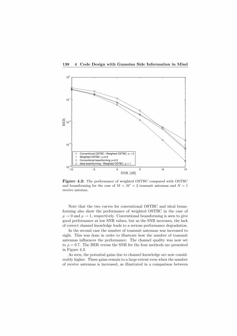
138 4 Code Design with Gaussian Side Information in Mind
−10 −5 0 5 10 1510−4
10−3
10−2
10−1
100
Conventional OSTBC / Weighted OSTBC: ρ→ 0Weighted OSTBC: ρ=0.9Conventional beamforming: ρ=0.9Ideal beamforming / Weighted OSTBC: ρ→ 1PSfrag replacements
BE
R
SNR [dB]
Figure 4.2: The performance of weighted OSTBC compared with OSTBCand beamforming for the case of M = M ′ = 2 transmit antennas and N = 1receive antenna.
Note that the two curves for conventional OSTBC and ideal beam-forming also show the performance of weighted OSTBC in the case ofρ → 0 and ρ → 1, respectively. Conventional beamforming is seen to givegood performance at low SNR values, but as the SNR increases, the lackof correct channel knowledge leads to a serious performance degradation.
In the second case the number of transmit antennas was increased toeight. This was done in order to illustrate how the number of transmitantennas influences the performance. The channel quality was now setto ρ = 0.7. The BER versus the SNR for the four methods are presentedin Figure 4.3.
As seen, the potential gains due to channel knowledge are now consid-erably higher. These gains remain to a large extent even when the numberof receive antennas is increased, as illustrated in a comparison between

4.9 Numerical Examples 139
−10 −8 −6 −4 −2 0 2 4 6 8 1010−6
10−5
10−4
10−3
10−2
10−1
100
Conventional OSTBC / Weighted OSTBC: ρ→ 0Weighted OSTBC: ρ=0.7Conventional beamforming: ρ=0.7Ideal beamforming / Weighted OSTBC: ρ→ 1PSfrag replacements
BE
R
SNR [dB]
Figure 4.3: The performance of weighted OSTBC compared with OSTBCand beamforming for the case of M = M ′ = 8 transmit antennas and N = 1receive antenna.
the proposed method and conventional OSTBC in Figure 4.4. Althoughnot presented, simulation results demonstrating significant gains werealso obtained for scenarios with fewer transmit antennas.
Varying the Channel Quality
The third and last case concerns how the channel quality affects the per-formance. Again, a system with two transmit antennas and one receiveantenna is considered. The SNR was fixed at 10 dB and the BER versusthe channel side information quality ρ was plotted. The result is shownin Figure 4.5, which thus provides an illustration of how the proposedscheme adapts to the variations in the channel quality. Hence, when thechannel quality is low weighted OSTBC is similar to conventional OS-
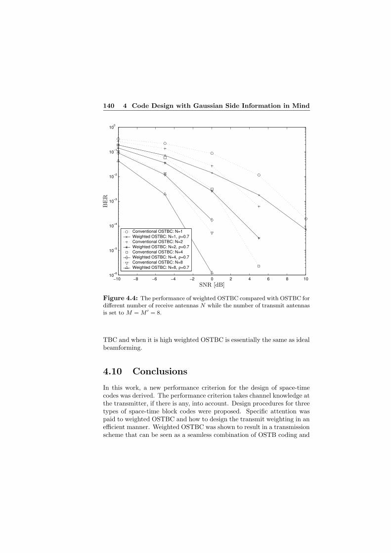
140 4 Code Design with Gaussian Side Information in Mind
−10 −8 −6 −4 −2 0 2 4 6 8 1010−6
10−5
10−4
10−3
10−2
10−1
100
Conventional OSTBC: N=1Weighted OSTBC: N=1, ρ=0.7Conventional OSTBC: N=2Weighted OSTBC: N=2, ρ=0.7Conventional OSTBC: N=4Weighted OSTBC: N=4, ρ=0.7Conventional OSTBC: N=8Weighted OSTBC: N=8, ρ=0.7PSfrag replacements
BE
R
SNR [dB]
Figure 4.4: The performance of weighted OSTBC compared with OSTBC fordifferent number of receive antennas N while the number of transmit antennasis set to M = M ′ = 8.
TBC and when it is high weighted OSTBC is essentially the same as idealbeamforming.
4.10 Conclusions
In this work, a new performance criterion for the design of space-timecodes was derived. The performance criterion takes channel knowledge atthe transmitter, if there is any, into account. Design procedures for threetypes of space-time block codes were proposed. Specific attention waspaid to weighted OSTBC and how to design the transmit weighting in anefficient manner. Weighted OSTBC was shown to result in a transmissionscheme that can be seen as a seamless combination of OSTB coding and

4.10 Conclusions 141
0 0.1 0.2 0.3 0.4 0.5 0.6 0.7 0.8 0.9 110−3
10−2
10−1
Conventional OSTBC / Weighted OSTBC: ρ→ 0Weighted OSTBCConventional beamformingIdeal beamforming / Weighted OSTBC: ρ → 1
PSfrag replacements
BE
R
ρ
Figure 4.5: Shows how the channel knowledge quality measure ρ affects theperformance. Weighted OSTBC is compared with OSTBC and beamformingfor a system with M = M ′ = 2 transmit antennas, N = 1 receive antenna anda fixed SNR=10 dB.
classical beamforming. The transmit weight design optimization problemwas proved to be convex for square transmit weighting matrices, implyingthat it can be solved in a reasonably efficient manner. Closed-form solu-tions were derived under certain asymptotic assumptions. Furthermore,the assumption of a simplified fading scenario was shown to result in aparticularly efficient optimization algorithm. Numerical results demon-strated significant gains over both an OSTBC system and a system usingconventional beamforming.

142 4 Code Design with Gaussian Side Information in Mind
Appendix 4.A Asymptotic Results
Our strategy for deriving the asymptotic results presented in Section 4.6is to make use of the fact that, under certain conditions, it is possible tointerchange the order of the limit and minimization operator, as exem-plified by
xas , lim%→a
arg minx∈X
V%(x)
= arg minx∈X
lim%→a
V%(x)
= arg minx∈X
V (x) ,
where X denotes the feasibility set and V (x) , lim%→a V%(x). From[SS89, p. 221] it follows that this holds if V%(x) converges uniformly in x
over X to the limit function V (x), X is a compact set (i.e., closed andbounded) and V (x) is continuous and has a unique global minimum.
To apply this theorem for the problem at hand, introduce a criterionfunction `′(Z) that is equal to the original criterion function `(Z|ζ), ex-cept for parameter independent terms and factors. Let ¯
i(Z) , lim `′(Z),where the limit will be taken as either ‖R−1
hh|h‖ → 0, η → 0, ‖Rhh|h‖ → 0
or η → ∞, depending on the asymptotic case under consideration. Theindex i is here used to number the four different cases. Assume for sim-plicity that M ′ = M throughout this appendix so that the rank constraintcan be disregarded. Moreover, define the set over which the parametersare optimized as
Z(ε) , Z|Z = Z∗ εIM , tr(Z) = Po . (4.42)
Clearly, the requirement that Z(ε) is compact is satisfied. Normally,ε is taken to be zero. The set in (4.42) then corresponds to the feasibilityset of the original optimization problem, as described by (4.26). However,in order to satisfy the requirement of a continuous limit function ¯
i(Z),we will for some of the cases first restrict Z(ε) by assuming that ε issmall and positive and then argue why we can let ε = 0 without affectingthe result. Proving that `′(Z) converges uniformly to ¯
i(Z) over Z(ε)amounts to showing that
lim supZ∈Z(ε)
|`′(Z) − ¯i(Z)| = 0 .
In order to simplify the notation, the original criterion function is for

4.A Asymptotic Results 143
the remaining part of this section written as
`(Z|ζ) = m∗R−1((IN ⊗ Zη) + R−1
)−1R−1m
− log det((IN ⊗ Zη) + R−1
),
where it is noted that η = µmin/(4σ2) is a quantity proportional to theSNR. Furthermore, recall that ‖X‖ = σmax, where σmax is the maximumsingular value of X. Keep also in mind that if the argument is a vector,the result is the usual vector norm.
4.A.1 Case 1: No Channel Knowledge
The first case that is considered is no channel knowledge, i.e., ‖R−1‖ → 0.Furthermore, it is assumed that ‖m‖ is bounded as ‖R−1‖ → 0.
To remove parameter independent terms in the limit function, theequivalent criterion function `′(Z) , `(Z|ζ) + MN log(η) is considered.For now, assume that ε > 0 so as to ensure that Z is invertible. Hence,`′(Z) can be written as
`′(Z) = m∗R−1((IN ⊗ Zη) + R−1
)−1R−1m
− log det(IMN + (IN ⊗ Zη)−1/2R−1(IN ⊗ Zη)−1/2
)
− log det (IN ⊗ Zη) + MN log(η) , (4.43)
where (·)1/2 is now a matrix square-root with Hermitian symmetry. Asshown below, this function converges uniformly in Z to the limit function
¯1(Z) , lim
‖R−1‖→0`′(Z) = − log det (IN ⊗ Zη) + MN log η
= −N log det(Z) . (4.44)
The limit function is obviously continuous. By utilizing Lagrangian mul-tipliers and an EVD of Z, it is straightforward to show that ¯
1(Z), subject
to Z ∈ Z(ε), has a unique global minimum Z(ζ)as = IMPo/M . This fact,
and the uniform convergence in Z over Z(ε), implies that, for a fixedpositive ε ≤ Po/M ,
Z(ζ)as = lim
‖R−1‖→0arg min
Z∈Z(ε)`′(Z) = IMPo/M . (4.45)
Note that the above development holds for arbitrarily small ε > 0and observe that the solution in (4.45) is independent of ε and does not
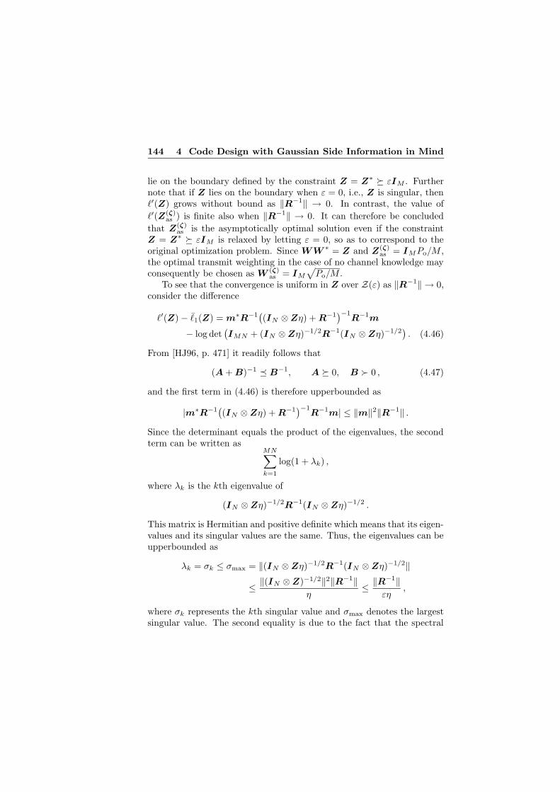
144 4 Code Design with Gaussian Side Information in Mind
lie on the boundary defined by the constraint Z = Z∗ εIM . Furthernote that if Z lies on the boundary when ε = 0, i.e., Z is singular, then`′(Z) grows without bound as ‖R−1‖ → 0. In contrast, the value of
`′(Z(ζ)as ) is finite also when ‖R−1‖ → 0. It can therefore be concluded
that Z(ζ)as is the asymptotically optimal solution even if the constraint
Z = Z∗ εIM is relaxed by letting ε = 0, so as to correspond to theoriginal optimization problem. Since WW ∗ = Z and Z(ζ)
as = IMPo/M ,the optimal transmit weighting in the case of no channel knowledge mayconsequently be chosen as W (ζ)
as = IM
√
Po/M .To see that the convergence is uniform in Z over Z(ε) as ‖R−1‖ → 0,
consider the difference
`′(Z) − ¯1(Z) = m∗R−1
((IN ⊗ Zη) + R−1
)−1R−1m
− log det(IMN + (IN ⊗ Zη)−1/2R−1(IN ⊗ Zη)−1/2
). (4.46)
From [HJ96, p. 471] it readily follows that
(A + B)−1 B−1, A 0, B 0 , (4.47)
and the first term in (4.46) is therefore upperbounded as
|m∗R−1((IN ⊗ Zη) + R−1
)−1R−1m| ≤ ‖m‖2‖R−1‖ .
Since the determinant equals the product of the eigenvalues, the secondterm can be written as
MN∑
k=1
log(1 + λk) ,
where λk is the kth eigenvalue of
(IN ⊗ Zη)−1/2R−1(IN ⊗ Zη)−1/2 .
This matrix is Hermitian and positive definite which means that its eigen-values and its singular values are the same. Thus, the eigenvalues can beupperbounded as
λk = σk ≤ σmax = ‖(IN ⊗ Zη)−1/2R−1(IN ⊗ Zη)−1/2‖
≤ ‖(IN ⊗ Z)−1/2‖2‖R−1‖η
≤ ‖R−1‖εη
,
where σk represents the kth singular value and σmax denotes the largestsingular value. The second equality is due to the fact that the spectral

4.A Asymptotic Results 145
norm is equal to the maximum singular value of its argument. An upperbound to the second term in (4.46) may be formed as
MN∑
k=1
log(1 + λk) ≤ MN log
(
1 +‖R−1‖
εη
)
. (4.48)
By utilizing the triangle inequality it is now clear that
supZ∈Z(ε)
|`′(Z) − ¯1(Z)| ≤ ‖m‖2‖R−1‖ + MN log
(
1 +‖R−1‖
εη
)
.
Since this expression, for a constant ε > 0 and a bounded m, obviouslytends to zero as ‖R−1‖ → 0, we have shown that `′(Z) converges uni-formly to ¯
1(Z) within the parameter set defined by Z(ε). This completesthe derivation for the no channel knowledge case.
4.A.2 Case 2: Infinite SNR
In the second case it is assumed that the SNR tends to infinity, i.e.,η = µmin/(4σ2) → ∞. Again, we start by assuming ε > 0. Similarly tothe previous case, an equivalent criterion function can be written as in(4.43), which also in this case converges uniformly in Z to
¯2(Z) , lim
η→∞`′(Z) = −N log det(Z) = ¯
1(Z) .
To see that the convergence is uniform, consider the two terms in (4.46).Utilizing (4.47), the first term is now upperbounded by
‖m‖2‖R−1‖2‖(IN ⊗ Zη)−1‖ ≤ ‖m‖2‖R−1‖2
εη,
whereas the upper bound of the second term is again given by (4.48).Hence, we have
supZ∈Z(ε)
|`′(Z) − ¯2(Z)| ≤ ‖m‖2‖R−1‖2
εη+ MN log
(
1 +‖R−1‖
εη
)
,
which obviously tends to zero as the SNR tends to infinity. The conver-gence is therefore uniform. The arguments following (4.45) then showthat the asymptotically optimal transmit weighting may once more bechosen as W (ζ)
as = IM
√
Po/M . This completes the derivation for thecase of infinite SNR.

146 4 Code Design with Gaussian Side Information in Mind
4.A.3 Case 3: Perfect Channel Knowledge
The third case concerns perfect channel knowledge in the sense that‖R‖ → 0. In addition, it is assumed that m , lim‖R‖→0 m exists and isfinite (with respect to some norm). For the present and the next case, itis possible to let ε = 0. The original constraints are therefore assumed.
Parameter independent terms and factors in the limit function areremoved by considering the equivalent criterion function
`′(Z) ,(`(Z|ζ) − log det(R) − m∗R−1m
)/η
= m∗(IMN + (IN ⊗ Zη)R
)−1R−1m/η
− log det(IMN + R1/2(IN ⊗ Zη)R1/2
)/η
− m∗R−1m/η . (4.49)
We start by showing that this function converges uniformly in Z to theobviously continuous limit function
¯3(Z) , lim
‖R‖→0`′(Z) = −m∗(IN ⊗ Z)m . (4.50)
The Taylor series [HJ96, p. 301],
(I − X)−1 =
∞∑
k=0
Xk,
which is valid if ‖X‖ < 1, is used for writing the first term in (4.49) as
m∗(
R−1 − (IN ⊗ Zη) +
∞∑
k=2
(− (IN ⊗ Zη)R
)kR−1
)
m/η .
By exploiting the triangle inequality and the formula for a geometricseries, an upper bound on the infinite sum, for sufficiently small η‖R‖,is obtained as
‖∞∑
k=2
(−(IN ⊗ Zη)R)kR−1‖ ≤∞∑
k=2
‖IN ⊗ Zη‖k‖R‖k−1
=‖IN ⊗ Zη)‖2‖R‖
1 − ‖IN ⊗ Zη‖‖R‖
=η2‖Z‖2‖R‖
1 − η‖Z‖‖R‖
≤ η2P 2o ‖R‖
1 − ηPo‖R‖ .

4.A Asymptotic Results 147
For the last inequality, the fact that ‖Z‖ ≤ Po has been used, which isdue to the trace constraint on Z. Now, let λk represent the kth eigenvalueof
R1/2(IN ⊗ Zη)R1/2 .
Since it then holds that
λk ≤ ‖R1/2‖2‖IN ⊗ Zη‖ = η‖R‖‖Z‖ ≤ ηPo‖R‖ ,
the second term in (4.49) is upperbounded by
MN log(1 + ηPo‖R‖)/η .
Finally, collecting the results for the first two terms yields
supZ∈Z(0)
|`′(Z) − ¯3(Z)| ≤ ηP 2
o ‖R‖‖m‖2
1 − ηPo‖R‖ + MN log(1 + ηPo‖R‖)/η .
The right hand side clearly tends to zero as ‖R‖ → 0. Hence, the con-vergence is uniform.
Changing the sign of the limit function in (4.50) and re-parameterizingusing Z = WW ∗ shows that the optimum of the limit function ¯
3(Z) isgiven by
W (ζ)as = arg max
W‖W ‖2
F=Po
m∗(IN ⊗ WW ∗)m . (4.51)
To solve this, let Ω , mm∗ and define
Θ ,
N∑
k=1
Ωk , (4.52)
where Ωk denotes the kth block of size M ×M on the diagonal of Ω. Thecost function in the above optimization problem can now be formulatedas
m∗(IN ⊗ WW ∗)m = tr((IN ⊗ WW ∗)Ω
)(4.53)
= tr(W ∗ΘW )
=(vec(Θ∗W )
)∗vec(W )
=(vec(W )
)∗(IM ⊗ Θ) vec(W ) ,
where the two last equalities are due to (C.1) and (C.2) in Appendix C,respectively. The power constraint is written on the form ‖ vec(W )‖ =√
Po.

148 4 Code Design with Gaussian Side Information in Mind
The optimization problem is readily solved utilizing the EVD of IM ⊗Θ. For this purpose, let λM denote the largest eigenvalue of Θ and recallthe assumption that it is strictly larger than all the other eigenvalues, i.e.,λM is unique. It can easily be verified that the eigenvalues of IM ⊗ Θare obtained by repeating the eigenvalues of Θ M times. Hence, λM isalso the largest eigenvalue of IM ⊗ Θ, with multiplicity M . The set ofoptimal solutions of (4.51) is therefore given by the eigenspace associatedwith λM . After introducing the complex-valued scalars µkM
k=1, thesolution can be written on the form
vec(W (ζ)as ) = µ1u1 + µ2u2 + · · · + uM (4.54)
where
u1 =
vM
00...0
,u2 =
0vM
0...0
, · · · ,uM =
0...00
vM
and vM are the eigenvectors of IM⊗Θ and Θ, respectively, correspondingto λM . Here, 0 is an M × 1 vector with all elements equal to zero. Using(4.54) all the solutions may also be expressed as
W (ζ)as =
[µ1vM µ2vM · · · µMvM
],
implying that Z(ζ)as = W (ζ)
as (W (ζ)as )∗ = vMv∗
M
∑Mk=1 |µk|2. Combining
this with the power constraint ‖W ‖2F = Po means that
∑Mk=1 |µk|2 =
Po, and hence Z(ζ)as = vMv∗
MPo. Consequently, regardless of the unit
norm vector vec(W (ζ)as ) chosen from the aforementioned eigenspace, it
holds that Z(ζ)as = vMv∗
MPo, which is thus a unique minimum pointof ¯
3(Z). Accordingly, the use of ¯3(Z) in the asymptotic analysis is
justified. Letting, for example, µ1 =√
Po, µ2 = · · · = µM = 0 andutilizing Z(ζ)
as = W (ζ)as (W (ζ)
as )∗, an asymptotically optimal solution isgiven by
W (ζ)as =
√
Po
[vM 0 · · · 0
].
As previously indicated, the solution is not unique. For example, per-muting the columns gives the same value of the cost function.
Recall that m = mh|ζ and R = Rhh|ζ . Note that (4.52) may also
be written on the form Θ = MH|ζM∗H|ζ , where MH|ζ is an M × N
matrix defined by the relation vec(MH|ζ) = mh|ζ , m = lim‖R‖→0 m.

4.A Asymptotic Results 149
Another equivalent way of defining MH|ζ is as the asymptotic MMSE
channel estimate MH|ζ , lim‖Rhh|ζ‖→0 E[H|ζ].
4.A.4 Case 4: Zero SNR
In the fourth case, the SNR is assumed to tend to zero, i.e., η → 0. Thederivation is to a large extent similar to the previous case. The Taylorexpansion,
log det(I + X) = tr(X) + O(‖X‖2) ,
where O(·) is the big ordo operator, is used to write the second term of(4.49) as
tr(R1/2(IN ⊗ Z)R1/2
)+ O(η) .
Combining this with (4.50) results in the limit function
¯4(Z) , lim
η→0`′(Z)
= −m∗(IN ⊗ Z)m − tr(R1/2(IN ⊗ Z)R1/2
). (4.55)
It is now evident from
supZ∈Z(0)
|`′(Z) − ¯4(Z)| ≤ ηP 2
o ‖R‖‖m‖2
1 − ηPo‖R‖ + |O(η)|
that the convergence is uniform. Thus, after changing the sign of ¯4(Z)
and parameterizing in terms of W , the cost function can be taken as
m∗(IN ⊗ WW ∗)m + tr(R1/2(IN ⊗ WW ∗)R1/2
).
Using the relation tr(AB) = tr(BA), this expression can be rewritten as
tr((IN ⊗ WW ∗)(mm∗ + R)
)= tr
((IN ⊗ WW ∗)Ω
), (4.56)
where now Ω , mm∗ + R. Finally, due to the similarity between (4.56)and (4.53), the development from the previous case shows that an asymp-totically optimal transmit weighting is given by
W (ζ)as =
√
Po
[vM 0 · · · 0
],
where vM is the eigenvector corresponding to the largest eigenvalueof Θ. Here, Θ is again defined as in (4.52). Note that an alter-native and perhaps more intuitive formulation of Θ is given by Θ =E[H|ζ] E[H|ζ]∗ + E[(H − E[H|ζ])(H − E[H|ζ])∗|ζ].
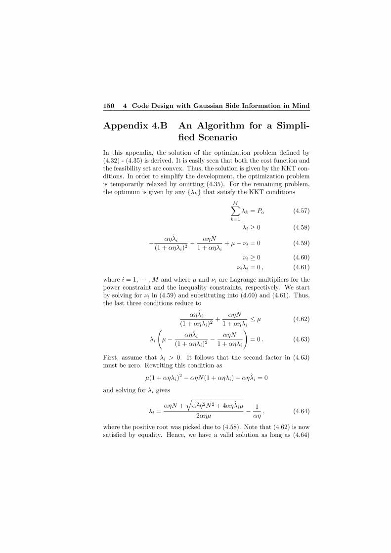
150 4 Code Design with Gaussian Side Information in Mind
Appendix 4.B An Algorithm for a Simpli-
fied Scenario
In this appendix, the solution of the optimization problem defined by(4.32) - (4.35) is derived. It is easily seen that both the cost function andthe feasibility set are convex. Thus, the solution is given by the KKT con-ditions. In order to simplify the development, the optimization problemis temporarily relaxed by omitting (4.35). For the remaining problem,the optimum is given by any λk that satisfy the KKT conditions
M∑
k=1
λk = Po (4.57)
λi ≥ 0 (4.58)
− αηλi
(1 + αηλi)2− αηN
1 + αηλi+ µ − νi = 0 (4.59)
νi ≥ 0 (4.60)
νiλi = 0 , (4.61)
where i = 1, · · · ,M and where µ and νi are Lagrange multipliers for thepower constraint and the inequality constraints, respectively. We startby solving for νi in (4.59) and substituting into (4.60) and (4.61). Thus,the last three conditions reduce to
αηλi
(1 + αηλi)2+
αηN
1 + αηλi≤ µ (4.62)
λi
(
µ − αηλi
(1 + αηλi)2− αηN
1 + αηλi
)
= 0 . (4.63)
First, assume that λi > 0. It follows that the second factor in (4.63)must be zero. Rewriting this condition as
µ(1 + αηλi)2 − αηN(1 + αηλi) − αηλi = 0
and solving for λi gives
λi =αηN +
√
α2η2N2 + 4αηλiµ
2αηµ− 1
αη, (4.64)
where the positive root was picked due to (4.58). Note that (4.62) is nowsatisfied by equality. Hence, we have a valid solution as long as (4.64)

4.B An Algorithm for a Simplified Scenario 151
gives a positive result and (4.57) is satisfied. On the other hand, for thecase of a non-positive result, we let λi = 0. That this indeed satisfies theKKT conditions is seen by verifying that (4.62) is true. Since
αηN +
√
α2η2N2 + 4αηλiµ
2αηµ− 1
αη≤ 0
and λi = 0 implies that
µ ≥ αηλi + αηN , (4.65)
it is obvious that all the KKT conditions, with the possible exception of(4.57), are satisfied. Finally, also (4.57) can be handled by writing theoptimal eigenvalues as
λi = max
0,
αηN +
√
α2η2N2 + 4αηλiµ
2αηµ− 1
αη
(4.66)
and then solving for µ in (4.57). It is apparent that (4.66) gives eigen-values that are sorted in ascending order. Therefore, the constraint thatwas initially omitted, i.e., (4.35), is automatically satisfied. Thus, (4.66)gives the optimal eigenvalues also for the original problem.


Chapter 5
Quantized ChannelFeedback: DesignApproach I
This chapter considers a wireless MIMO communication link in which thetransmitter has access to quantized channel side information obtainedfrom the receiver via a dedicated feedback link. The focus is on weightedOSTBC, although the methods to be developed herein are applicable toall three code structures mentioned in Section 3.2. Suitable transmitweighting matrices are designed by modifying the previously developedtransmit weight design procedure in a heuristic manner to better copewith quantized channel knowledge. An alternative and mathematicallycleaner technique for dealing with quantized channel feedback will bedescribed in Chapter 6.
Feedback delay, quantization errors and feedback channel bit-errorsare all assumed to impair the quality of the channel side information.To reduce these errors, methods based on vector quantization for noisychannels are used in the design of the feedback link. The proposed trans-mission scheme and feedback link takes the non-perfect nature of thechannel information into account while combining the benefits of conven-tional beamforming with those given by OSTB codes in a similar man-ner as in Chapter 4. Simulation results for a spatially uncorrelated flatRayleigh fading scenario with two transmit antennas and one receive an-tenna demonstrate significant gains over conventional methods, including

154 5 Quantized Channel Feedback: Design Approach I
robustness to feedback channel bit-errors.
5.1 Introduction
Recently, space-time codes [GFBK99, TSC98, TJC99] have been devel-oped that utilize both the spatial and temporal dimensions for increasingthe performance of a wireless communication link where the transmitteris equipped with multiple antennas. A potential drawback with classicalspace-time codes is that they are designed under the assumption that thetransmitter does not know the channel. Hence, even if channel knowl-edge is available, it is not used for improving the performance. In somecommunication systems it is reasonable to assume that such channel sideinformation is in fact available. Both TDD systems and FDD systemsequipped with a feedback link belong to this category. In the formercase the channel may be estimated in the receive mode and then oftenassumed to be the same for the transmit mode, whereas for the lattercase channel estimates are obtained at the receiver and then transportedover a dedicated feedback link to the transmitter.
A common way of utilizing channel side information is to make useof beamforming techniques for maximizing the received energy, essen-tially steering the transmission in the direction of the receiver. Therehas recently been a growing interest on the use of feedback informa-tion in conjunction with transmission methods related to beamforming[Wit95, NLTW98, HP98, MSA01, VM01, OGDH01, HW01]. The factthat beamforming based on channel information from a feedback link isused in the closed-loop mode of the WCDMA system further illustratesthe practical significance of such schemes [3GP02b, DGI+02].
To keep the wireless system spectrally efficient, the channel informa-tion is often heavily quantized prior to being transported over the feed-back link. Needless to say, the channel knowledge at the transmitter istypically far from perfect. Not only quantization may degrade the qualityof the channel information. The quality often suffers from a delay in thefeedback link, which means that the channel information is, due to thetime-varying nature of the wireless channel, more or less outdated by thetime it reaches the transmitter [OGDH01, HW01]. Bit-errors introducedby the channel over which the feedback link operates may also severelyimpair the performance.
In order to mitigate the detrimental consequences of errors in thechannel information, space-time codes can be combined with beamform-

5.1 Introduction 155
ing type of schemes, as evident from previous chapters in this thesis. Theidea is to make use of the complementary strengths of both transmissionmethodologies. Traditional space-time codes [GFBK99, TSC98, TJC99]are designed to operate without any channel knowledge and hence providethe system with a basic level of performance in the absence of reliablechannel state information at the transmitter. Beamforming, on the otherhand, is advantageous when the channel knowledge is reliable. WeightedOSTBC in conjunction with the transmit weight design procedure devel-oped in Section 4.5 constitutes a particularly attractive combination ofspace-time coding and beamforming.
In this work, we consider the use of weighted OSTBC in a MIMOwireless communication link where the transmitter has access to quan-tized channel side information obtained from the receiver via a dedicatedfeedback link. Suitable transmit weighting matrices are constructed byutilizing the transmit weight design procedure in Section 4.5. However,since that design procedure was developed primarily with Gaussian chan-nel side information in mind, it does not perform well in its original formwhen the channel information is heavily quantized. To obtain betterperformance, heuristic modifications to the original design procedure areproposed in this chapter. The design of the feedback link is also addressedand specifically tailored to suit the characteristics of weighted OSTBC.
In addition to feedback delay related errors covered by the methodsof the previous chapter, the system under study is assumed to sufferfrom errors in the channel information due to quantization and feed-back channel bit-errors. By designing the feedback link based on vectorquantization (VQ) for noisy channels [Far90, FV91], the damaging effectscaused by these errors are successfully avoided. Two different types offeedback links are investigated. In the first type, the channel coefficientsare quantized directly, like in standard VQ, while in the second type theamplitude and phase are first separated and then quantized. The remain-ing errors are taken into account by the transmit weight design proce-dure. Previous work dealing with quantized channel information includes[NLTW98, HP98, MSA01]. However, these papers differ substantiallyfrom the present work since they study conventional beamforming andsee quantization errors as the only error source1. Numerical examples fora spatially uncorrelated flat Rayleigh fading scenario with two transmit
1The work in [NLTW98] does in fact also consider errors that can be described bymodeling the channel side information as correlated with the true channel. However,that case is studied separately from the case of quantized channel information, notjointly as herein.
156 5 Quantized Channel Feedback: Design Approach I
antennas and one receive antenna show the robustness against channelinformation impairments of the proposed setup compared with systemswhich tentatively assume the channel information at the transmitter tobe perfect.
The main contribution in this chapter is the development and studyof a transmission method and feedback designs that, used together, arerobust against feedback delay, quantization and feedback channel bit-errors. We show how weighted OSTBC can utilize quantized feedbackinformation and also introduce the use of vector quantization for noisychannels into the design of the feedback link. In addition, detectionof the transmit weighting matrix at the receiver is treated. The setupconsidered in this work may be motivated by current standardizationproposals for the WCDMA system. For example, an OSTB code is usedin the open-loop mode, whereas in the closed-loop mode the receiverinforms the transmitter about the appropriate transmit antenna weightsbased on heavily quantized channel estimates [3GP02a, 3GP02b].
The chapter is organized as follows. Section 5.2 presents the systemmodel including a generic overview of the feedback link. A so-called sim-plified fading scenario is also described for later reference. In Section 5.3,the transmit weight design procedure of the previous chapter is used todetermine a suitable codebook of transmit weights. The design of thetwo types of feedback links is treated in Section 5.4. In Section 5.5, amethod for detecting the transmit weighting at the receiver is developed.Finally, based on the simplified fading scenario, numerical examples arepresented in Section 5.6.
5.2 System Model
This work considers a MIMO wireless communication system that utilizesweighted OSTBC based on quantized channel side information ζ obtainedfrom a feedback link. An illustration of the system under consideration isgiven in Figure 5.1. As seen, the side information is used for choosing atransmit weighting W = W (ζ) out of a fixed codebook W (ζ) of weightscorresponding to all possible outcomes of ζ. Methods for designing theweighting matrices so as to take the available channel knowledge intoaccount are described later in the chapter.
The generic system model and the assumptions regarding code struc-tures described in Section 3.1 still apply. Hence, there are M trans-mit and N receive antennas and the received signal vector is given by

5.2 System Model 157
PSfrag replacements
......OSTB
Encoder Wc(n)c(n) x(n)
MM ′ NReceiver
...
Pre-Proc.
Enc: ε(·)Dec: δ(j) Pj|i
ij
H⇔h=vec(H)︷ ︸︸ ︷
γ
ζ
W (ζ)
W = W (ζ)
Figure 5.1: Overview of a MIMO system where weighted OSTBC isused in conjunction with quantized channel side information ζ obtainedfrom a feedback link.
x(n) = H∗c(n)+e(n), where the M×N matrix H represents the MIMOchannel, c(n) the transmitted vector at sample index n and e(n) is a noiseterm generated from a spatially and temporally white complex Gaussianprocess. The resulting received block of vectors, corresponding to a trans-mitted codeword of length L, can be written as X = H∗C + E. Sinceweighted OSTBC is used, it follows from (3.6) that the transmitted code-word C ∈ C = CkK
k=1 is given by C = WC, where C ∈ C = CkKk=1
is the codeword output from the OSTB encoder. Hence,
X = H∗C + E = H∗WC + E , (5.1)
where the variance of each element of the noise matrix E is equal to σ2.All codewords in C are assumed equally probable. From (3.15), it followsthat the average output power per information bit, conditioned on thechannel side information ζ, is limited to P by the power constraint
‖W (ζ)‖2F = Po , (5.2)
where Po , P log2(K)/Lo.Although the transmit weighting matrix W may contain more
columns than rows so as to map an OSTB code designed for a smallantenna array to a larger array, the focus in the present work is on thecase when W is square, i.e., M = M ′. If desired, the methods to bedeveloped herein are easily extended to handle also the case of M ′ < M .
To model the fading, the channel vector h , vec(H) with elementshk is assumed to obey a complex Gaussian distribution described by

158 5 Quantized Channel Feedback: Design Approach I
the mean vector mh , E[h] and the covariance matrix Rhh , E[(h −mh)(h − mh)∗]. This is a flexible fading model that can handle bothspatially uncorrelated Rayleigh fading as well as more realistic scenarioswith correlated fading.
It will be convenient to have a measure of the quality of the chan-nel side information. Since the channel information is quantized, h|ζis not complex Gaussian distributed. Hence, unlike in Section 4.2, theconditional covariance Rhh|ζ , E[(h − mh|ζ)(h − mh|ζ)∗|ζ] does notprovide a complete description of the remaining uncertainty in h whenthe channel information ζ is known. Nevertheless, it is clear that it con-stitutes a measure of the reliability of the channel side information. Inparticular, perfect channel information corresponds to ‖Rhh|ζ‖ → 0, as-suming a fixed ζ. The other extreme of no channel knowledge is definedas a scenario in which ζ is independent of h (so that mh|ζ = mh andRhh|ζ = Rhh) and the fading is non-informative, i.e., mh is zero andRhh is a scaled identity matrix. This is a reasonable definition, since, asalso pointed out in Section 4.8, the symmetrical nature of the statisticaldistribution of the channel means that all transmit directions are equallygood.
5.2.1 An Overview of the Feedback Link
A feedback link is assumed to provide the transmitter with estimates ofthe current channel realization. In a typical such system, it is desirableto keep the data rate over the feedback link to a minimum in order forthe whole system to be spectrally efficient. This often means that thechannel estimates must be heavily quantized, which in turn results in aconsiderable amount of quantization errors. Feedback channel bit-errorsand feedback delay may also plague the channel information. To handlethese additional problems, we propose the use of techniques related to VQfor noisy channels [Far90, FV91], which take into account that the channelbetween the encoder and decoder may introduce bit-errors. Based onsuch procedures, two different types of feedback links are designed inSection 5.4.
In order to model feedback delay, it is assumed that the channel co-efficients transmitted over the feedback link are correlated (to an ar-bitrary degree) with the true channel. As illustrated in Figure 5.1,these channel coefficients are contained in the MN × 1 initial channelinformation vector γ, with elements γk. The vectors γ and h areassumed to be jointly complex Gaussian distributed. Let mγ , E[γ]

5.2 System Model 159
represent the mean of γ and let Rhγ , E[(h − mh)(γ − mγ)∗] and
Rγγ , E[(γ − mγ)(γ − mγ)∗] denote the relevant cross-covariance ma-trix and covariance matrix, respectively. Since γ and h are correlated, γ
can be thought of as representing an earlier copy of the true channel h, inaccordance with the well-known Jakes model [Jak94], which may be usedto describe the time-variations of the channel as a temporally correlatedstationary complex Gaussian process. Loosely speaking, the correlationproperties determine the quality of the initial channel information. An-other, more precise, measure is to again use the conditional covariance,in this case Rhh|γ , E[(h−mh|γ)(h−mh|γ)∗|γ], where mh|γ , E[h|γ],similarly to as when a quality measure for ζ was defined.
As seen in Figure 5.1, the initial channel information γ may, depend-ing on the type of feedback link, be pre-processed2 prior to being inputto the encoder. For the sake of notational brevity, the remaining part ofthis section assumes that the pre-processing stage is absent. The purposeof the encoder is to map each input source vector γ to a correspondinginteger i. Since the feedback link is assumed to use b bits for the quan-tization, the encoder is a mapping ε : C
NM → 0, · · · , 2b − 1 such thatε(γ) = i for an input vector γ. The mapping of the encoder is described
by γ ∈ Si ⇒ ε(γ) = i, where the set S i2b−1i=0 of encoder regions defines
a partition of CNM .
The encoder output i is mapped into bits which are then transmittedover what is here modeled as a memoryless binary symmetric channelwith bit-error probability Pb. After passing through the feedback chan-nel, the resulting b bits are mapped into an index j representing the out-put of an equivalent memoryless discrete multilevel input-output channelwith transition probabilities Pj|i , Pr[j|i], (i, j) ∈ 0, · · · , 2b − 12.Let dh(i, j) denote the number of bits in which the bit-patterns of i andj differ, the so-called Hamming distance. Since the binary channel is
memoryless, it is clear that Pj|i = Pdh(i,j)b (1 − Pb)b−dh(i,j).
The output j from the feedback channel is used by the feedback de-coder for reconstructing the current channel realization or a related quan-tity. More precisely, the decoder performs a mapping such that ζ = δ(j)
for the discrete feedback channel output j. The codebook δ(j)2b−1j=0
thus defines the decoder, where δ(j) represents an estimate of the cur-rent channel realization (or related quantity). Based on the outcome ofζ, the transmit weighting W currently in use is chosen, out of a fixed
2Although not considered in this work, pre-processing may include predicting thecurrent channel h based on several earlier channel estimates.
160 5 Quantized Channel Feedback: Design Approach I
codebook W (ζ) of 2b possibly different weights, as W = W (ζ).
It should now be clear that the feedback decoder and the subsequentblock containing the codebook W (ζ) may be merged into a single equiv-alent device with input j and output W . The merged device determines
the transmit weighting as W = W(j)
based on an equivalent codebook
W (j)2b−1j=0 , where W
(j), W (δ(j)). Thus, the codebook is directly
indexed by the feedback channel output j. This is actually how thetransmission scheme would be implemented in practice. The feedbackdecoder δ(j) is here included in the system model only because it willturn out to be useful from a conceptual standpoint when later designingthe quantization scheme.
The transmission scheme and the feedback link rely on certain pa-rameters. Because of this, both the transmitter and receiver are assumedto know mh, mγ , Rhh, Rhγ , Rγγ , σ2 and Pb, which typically varymuch slower than the channel matrix. Hence, they can be updated ata relatively low rate, considerably simplifying their distribution over thesystem.
Note that the transmission scheme and the feedback link are in thiswork designed separately, i.e., the goal is to first design the feedbacklink such that a good channel estimate is obtained and then determinea suitable transmit weighting based on this estimate. Another possibleapproach is of course to design the transmission scheme and the feedbacklink jointly. The codebook would in this case contain the transmit weights
explicitly, like in the equivalent codebook W (j)2b−1j=0 . Preliminary re-
sults in this direction may be found in our work in [JSO02b]. However,a major problem with such a joint approach, which motivates the sepa-rate design strategy considered in the present work, is that training thequantizer represents a highly computationally demanding optimizationproblem.
5.2.2 A Simplified Fading Scenario
The present section describes a simple special case of the previously dis-cussed scenario with arbitrary complex Gaussian fading. As will be ev-ident from below, this simplified fading scenario corresponds to the onepresented in Section 4.8 but now with a notation that complies with theproblem at hand.
In the simplified fading scenario, a rich scattering environment is con-sidered in which the antennas at both the transmitter and the receiver

5.3 Determining the Weighting Matrices 161
are spaced sufficiently far apart so that the fading becomes independent.Adhering to the usual assumptions in the space-time coding literaturea spatially uncorrelated Rayleigh fading scenario is considered, i.e., thechannel coefficients hk are modeled as zero-mean IID complex Gaus-sian with variance equal to σ2
h. In view of the well-known Jakes fadingmodel [Jak94] and since the initial channel information γ is consideredto be a delayed copy of the current channel realization, we make thereasonable assumption that h and γ are jointly complex Gaussian andequally distributed. See the discussion concerning feedback delay in Sec-tion 4.2.1 for a more detailed motivation as to why such an assumptionmakes sense.
Each initial channel information coefficient γk is correlated with thecorresponding current channel coefficient hk and uncorrelated with allothers. The degree of correlation is given by the normalized correlationcoefficient ρ , E[hkγ∗
k ]/σ2h. Thus, the distribution of the current channel
and the initial channel information is characterized by
mh = 0, mγ = 0
Rhh = σ2hIMN , Rγγ = σ2
hIMN , Rhγ = σ2hρIMN .
From the above and from standard results in estimation theory [Kay93,p. 509] it follows that
mh|γ = E[h|γ] = ργ
Rhh|γ = E[(h − mh|γ)(h − mh|γ)∗|γ] = σ2h(1 − |ρ|2)IMN .
Let ρ , |ρ| play the role of a separate quality measure for the initialchannel information, in the case of the present simplified fading scenario.Based on such a quality measure, perfect initial channel information andno initial channel information correspond to ρ → 1 and ρ → 0, respec-tively. Obviously, the former definition complies with ‖Rhh|γ‖ → 0,while the latter definition corresponds to the previously mentioned caseof non-informative fading statistics.
5.3 Determining the Weighting Matrices
Recall that weighted OSTBC utilizes the channel side information forimproving a predetermined OSTB code by means of a transmit weightingW = W (ζ). As previously explained, the weighting is here obtained froma fixed codebook W (ζ) of 2b possibly different weighting matrices. The

162 5 Quantized Channel Feedback: Design Approach I
strategy in the present chapter for constructing a suitable codebook is toutilize the transmit weight design procedure developed in Section 4.5 fordetermining the W (ζ)’s.
One drawback with such an approach is that the underlying designprocedure is not developed specifically for quantized channel side infor-mation. Indeed, it is based on the assumption that the channel h condi-tioned on the channel side information ζ is complex Gaussian. Such anassumption may in some cases be a good approximation of the statisticalrelation between h and ζ, particularly if the number of bits used for thequantization is high and the feedback channel does not introduce any bit-errors. This asymptotic argument provides motivation for the strategyconsidered herein despite the fact that the complex Gaussian assumptionis not perfectly valid. Depending on the type of feedback link, the designprocedure may need to be modified in a heuristic manner so as to bettersuit the characteristics of the quantized channel feedback. In any case,the resulting transmission schemes are clearly suboptimal, but still usefulas later numerical examples will show.
Applying the above design strategy means that the codebook of trans-mit weights is obtained based on the design procedure in (4.25), tailoredto the problem at hand, to arrive at
W (ζ) = arg minW
‖W‖2F=Po
˜(W ;m(ζ),R(ζ)), ζ = δ(j), ∀j , (5.3)
where
˜(W ;m,R) , m∗R−1((IN ⊗ WW ∗)µmin/(4σ2) + R−1
)−1R−1m
− log det((IN ⊗ WW ∗)µmin/(4σ2) + R−1
). (5.4)
As seen, the transmit weight design procedure in (5.3) is formulatedin a somewhat different manner than what was done for the originalprocedure in (4.25). Compared with (4.25), two new parameters m(ζ),R(ζ) now replace the conditional mean mh|ζ and covariance Rhh|ζ , re-spectively. Both m(ζ) and R(ζ) are determined from the output of thefeedback link, as explained in the following section where two differenttypes of feedback links will be investigated. This modified notation servesto emphasize that the two parameters will not always represent the con-ditional mean and covariance.
Techniques for efficiently solving the numerical optimization problemposed by (5.3) were given in Section 4.5. Since the channel feedback isquantized, the transmit weights may be predetermined by designing them

5.4 Feedback Link Design 163
off-line. As a result, the optimization problem in (5.3) is considered solvedin the following.
5.4 Feedback Link Design
This section describes the design of two different feedback links. Bothprovide the transmitter with quantized channel information. The firsttype employs an encoder that quantizes the channel coefficients directly.It is an uncomplicated design which serves to illustrate the problem andstands on solid theoretical grounds. A drawback is that it wastes bitsas simulation results in Section 5.6 will show. To remedy this deficiency,modifications of the basic concept, to some extent based on heuristicarguments, are utilized in the design of the second feedback link. In par-ticular, the channel coefficients are re-mapped prior to the quantizationso that the required number of bits is reduced.
Regardless of the type of feedback link, the feedback encoder anddecoder are optimized with the aim of minimizing the total distortiondue to quantization, feedback delay and feedback channel bit-errors. Thisis accomplished by using appropriately modified design techniques takenfrom the field of vector quantization for noisy channels. Although theVQ design is computationally demanding, it may be performed off-lineand the result can be stored in lookup tables for quick real-time access.Thus, for a moderate number of bits b, the overall real-time complexityof the feedback link must be considered low.
5.4.1 Feedback Link Type I – Direct Quantization
In the first feedback link that is considered, the channel coefficients aredirectly quantized. This is illustrated in Figure 5.2, where the initialchannel information vector γ is input to the encoder. Hence, no pre-processing of γ is performed. The decoder is seen to output an estimateh(j) , δ(j) of the true channel h. The estimate, which constitutes thechannel information ζ, is not explicitly used by the transmitter. Rather,it is an imaginative output used only for designing a good encoder-decoderpair that in turn produces suitable feedback information. After designingthe feedback link, the parameters m(ζ) and R(ζ), needed in the transmitweight design procedure, may be determined based on the feedback linkoutput h(j).
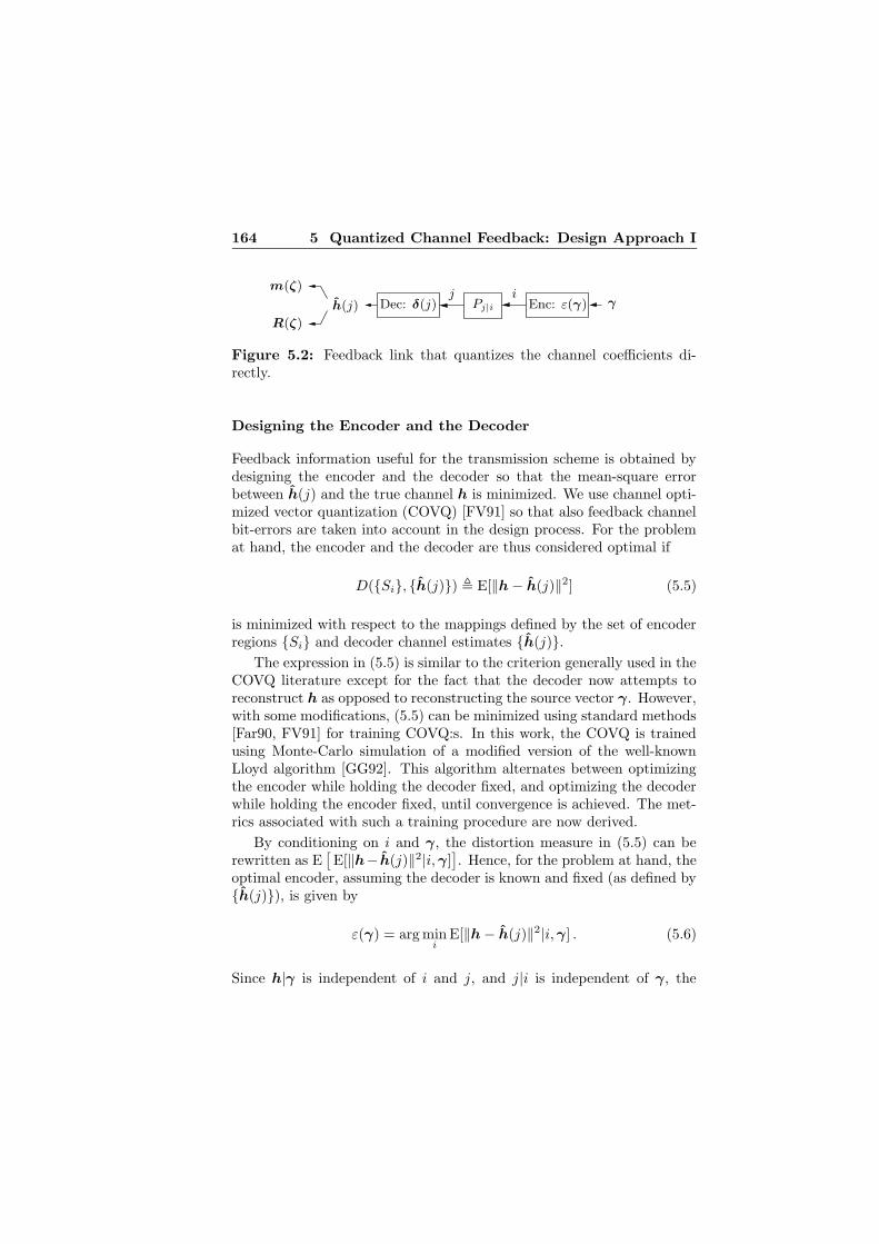
164 5 Quantized Channel Feedback: Design Approach I
PSfrag replacements
Enc: ε(γ)Dec: δ(j) Pj|i
ijγh(j)
m(ζ)
R(ζ)
Figure 5.2: Feedback link that quantizes the channel coefficients di-rectly.
Designing the Encoder and the Decoder
Feedback information useful for the transmission scheme is obtained bydesigning the encoder and the decoder so that the mean-square errorbetween h(j) and the true channel h is minimized. We use channel opti-mized vector quantization (COVQ) [FV91] so that also feedback channelbit-errors are taken into account in the design process. For the problemat hand, the encoder and the decoder are thus considered optimal if
D(Si, h(j)) , E[‖h − h(j)‖2] (5.5)
is minimized with respect to the mappings defined by the set of encoderregions Si and decoder channel estimates h(j).
The expression in (5.5) is similar to the criterion generally used in theCOVQ literature except for the fact that the decoder now attempts toreconstruct h as opposed to reconstructing the source vector γ. However,with some modifications, (5.5) can be minimized using standard methods[Far90, FV91] for training COVQ:s. In this work, the COVQ is trainedusing Monte-Carlo simulation of a modified version of the well-knownLloyd algorithm [GG92]. This algorithm alternates between optimizingthe encoder while holding the decoder fixed, and optimizing the decoderwhile holding the encoder fixed, until convergence is achieved. The met-rics associated with such a training procedure are now derived.
By conditioning on i and γ, the distortion measure in (5.5) can berewritten as E
[E[‖h− h(j)‖2|i,γ]
]. Hence, for the problem at hand, the
optimal encoder, assuming the decoder is known and fixed (as defined byh(j)), is given by
ε(γ) = arg mini
E[‖h − h(j)‖2|i,γ] . (5.6)
Since h|γ is independent of i and j, and j|i is independent of γ, the

5.4 Feedback Link Design 165
criterion function in (5.6) can be expanded as
E[‖h − h(j)‖2|i,γ] =2b−1∑
j=0
Pr[j|i,γ] E[(
h − h(j))∗(
h − h(j))∣∣i, j,γ
]
=2b−1∑
j=0
Pj|i E[h∗h − h∗h(j) − h(j)∗h + h(j)∗h(j)|i, j,γ]
=2b−1∑
j=0
Pj|i
(E[h∗h|γ] − E[h|γ]∗h(j) − h(j)∗ E[h|γ] + h(j)∗h(j)
)
=2b−1∑
j=0
Pj|i
(mh|γ − h(j)
)∗(mh|γ − h(j)
)− m∗
h|γmh|γ + E[h∗h|γ] ,
where we note that mh|γ = E[h|γ] is the MMSE estimate of the currentchannel realization h based on γ. The assumption that h and γ arejointly complex Gaussian implies that mh|γ is given by
mh|γ = mh + RhγR−1γγ(γ − mγ) .
After omitting terms independent of i, (5.6) simplifies to
ε(γ) = arg mini
2b−1∑
j=0
Pj|i‖mh|γ − h(j)‖2 . (5.7)
Now we turn to the decoder. Since a mean-square error criterion isused, standard results from estimation theory imply that the optimaldecoder, given a known encoder (as described by the encoder regionsSi), is obtained as δ(j) = h(j) = E[h|j]. By again utilizing that h|γis independent of i and j and, moreover, that γ|i is independent of j, thedecoder is derived as
δ(j) = h(j) = E[h|j]
=
2b−1∑
i=0
Pr[i|j] E[h|i, j]
=2b−1∑
i=0
Pi|j E[E[h|γ, i, j]|i, j]

166 5 Quantized Channel Feedback: Design Approach I
=
2b−1∑
i=0
Pi|j E[mh|γ |i] (5.8)
where
E[mh|γ |i] = mh + RhγR−1γγ(E[γ|i] − mγ)
Pi|j ,Pj|iPi
∑2b−1i=0 Pj|iPi
,
with Pi denoting the probability that the feedback encoder outputs i.As seen, the channel knowledge contained in γ is incorporated into
the feedback link design through the MMSE estimate mh|γ . This makessense since the goal is to reproduce the current channel h, as opposed toreproducing the source vector γ like in standard COVQ. Note that whenthe MMSE estimate is perfect, so that mh|γ is essentially the same as h,the feedback link simplifies to a standard COVQ (as can be verified bysetting h in place of mh|γ).
Feedback delay, quantization errors and bit-errors in the feedbackchannel all contribute to the non-perfect nature of the channel informa-tion. This is also reflected by the fact that, as shown in Appendix 5.A.1,Rhh|ζ , which is a measure of the quality of the channel side information
ζ = h(j), can be decomposed into three corresponding terms accordingto
Rhh|ζ = Rhh|γ + RhγR−1γγ E[(γ − E[γ|i])(γ − E[γ|i])∗|j]R−1
γγR∗hγ
+ RhγR−1γγ E
[(E[γ|j] − E[γ|i])(E[γ|j] − E[γ|i])∗
∣∣j]R−1
γγR∗hγ , (5.9)
where the first term can be interpreted as feedback delay distortion (i.e.,h and γ differ), the second term can be thought of as describing thecontribution from quantization errors and the third term corresponds tothe feedback channel distortion.
Determining m(ζ) and R(ζ)
To construct the codebook of transmit weights, m(ζ) and R(ζ) need tobe determined for each of the 2b possible outcomes of the channel sideinformation vector ζ = δ(j) = h(j). For the present type of feedbacklink, we let m(ζ) , mh|ζ , R(ζ) , Rhh|ζ , in line with the setup of theoriginal design procedure. In case of an ideal feedback channel, this choiceessentially corresponds to modeling the quantization errors as complex
5.4 Feedback Link Design 167
Gaussian. As pointed out in Section 4.2.1, such a model represents arather crude approximation.
Since it can be assumed that there is a one to one correspondencebetween h(j) and j, the required entities are given by
m(ζ) = mh|ζ = E[h|j] = h(j)
R(ζ) = Rhh|ζ = E[(h − E[h|j])(h − E[h|j])∗|j]= E[hh∗|j] − E[h|j] E[h|j]∗
= Rhh|γ + RhγR−1γγ(E[γγ∗|j] − E[γ|j] E[γ|j]∗)R−1
γγR∗hγ ,
where
E[γ|j] =2b−1∑
i=0
Pi|j E[γ|i], E[γγ∗|j] =2b−1∑
i=0
Pi|j E[γγ∗|i] .
A more detailed derivation can be found in Appendix 5.A. To implement(5.7) and (5.8) in the VQ design process, and also to compute m(ζ) andR(ζ), the entities Pi, E[γ|i] and E[γγ∗|i] are all replaced by appropriatesample estimates obtained from the Monte-Carlo simulation. The trans-mit weight design procedure in (5.3) is thereafter used for obtaining the
codebook W (ζ).
Parameter Independent Encoder/Decoder
Clearly, the COVQ depends on a number of parameters related to thejoint statistics of h and γ. From (5.7), (5.8) and the expression formh|γ it is obvious that mh, mγ , Rhγ and Rγγ directly influence theCOVQ. In practice, this may be handled by appropriately quantizing theparameters and designing several COVQ:s off-line, one for each possiblerealization of the quantized parameters.
Such an approach may be undesirable for complexity reasons. Hence,it would be attractive if the encoder-decoder pair could be held fixed,regardless of the value of these parameters and without loss of perfor-mance. Toward this end, note that the dependence upon mh and mγ isonly superficial and can easily be removed. Because of the expression formh|γ , it is straightforward to show that the COVQ can be trained as-suming that h and γ are zero-mean vectors, without loss of performance.Consequently, to implement the COVQ, mh is added to the output ofthe decoder and γ − mγ is used as input to the encoder.

168 5 Quantized Channel Feedback: Design Approach I
In general, the COVQ still depends on Rhγ and Rγγ . However, whenthese are equal to scaled identity matrices, it can be shown that also theremaining dependence can be removed. Thus, for the simplified fadingscenario the structure of the feedback link reduces to the one illustratedin Figure 5.3. Without loss of performance, the feedback link is trainedusing ρ → 1 and σ2
h = 1 and is then held fixed. The resulting encoder-decoder pair is used also for other values of ρ and σ2
h by normalizing the
input to the encoder and computing the channel estimate h(j) as theproduct of the output of the decoder and the true value of ρσh.
PSfrag replacements
Enc: ε(γ)Dec: δ(j) Pj|iij
γh(j)
m(ζ)
R(ζ)1/σh
ρσh
Figure 5.3: Equivalent structure of feedback link for the simplified fad-ing scenario.
Behavior of Weighted OSTBC Based on Quantized Feedback
The transmission scheme and the feedback link cooperate so that robust-ness against channel information impairments is achieved. To understandwhat makes the system successful, this section discusses the behavior ofthe transmission scheme and the feedback link in the two extreme casesof perfect and no channel knowledge, respectively. The discussion is to alarge extent also applicable to the second type of feedback link which ispresented in Section 5.4.2.
Perfect channel knowledge corresponds to ‖R(ζ)‖ = ‖Rhh|ζ‖ → 0,which means that m(ζ) = mh|ζ is essentially equal to the true channelvector h. By studying the expression for Rhh|ζ in (5.9) it is realized thatin order for the feedback link to output perfect channel information, allof the three error sources must be absent. If this is the case, the first termof the design criterion in (5.4) is seen to dominate. From the previousanalysis in Section 4.6, it is clear that this means that the designed trans-mit weighting is a rank one matrix such that the all the output poweris allocated to the transmit-direction given by the strongest left singulareigenvector of the channel matrix H. The transmitter is hence seen toperform a sort of beamforming. In particular, in the case of only onereceive antenna it holds that H = h, which implies that the strongestleft singular eigenvector is proportional to h. Hence, all the output power

5.4 Feedback Link Design 169
is concentrated in the direction of the current channel realization. It canthus be concluded that when the initial channel information is good, alarge number of bits b are used, the feedback channel bit-error probabil-ity Pb is small and only one receive antenna is present, the transmissionscheme resembles classical beamforming.
Consider now the other extreme of no channel knowledge. In otherwords, ζ is independent of h and the channel fading is non-informativeso that mh = 0 and Rhh = σ2
hIMN , as is for example the case in thesimplified fading scenario in Section 5.2.2. Clearly, ζ is independent of h
if there is no initial channel information (i.e., ρ = 0 or γ is independent ofh), Pb = 0.5 and/or b = 0. It readily follows that m(ζ) = mh|ζ = mh =0 and R(ζ) = Rhh|ζ = Rhh = σ2
hIMN . From the previous developmentin Section 4.8.1 it is now evident that the designed transmit weighting is ascaled unitary matrix, for example W = IM
√
Po/M . The predeterminedcodewords in C are hence transmitted without modification, resulting inan open-loop type of system employing conventional OSTBC. This makessense since the transmitter does not know the channel and therefore hasto choose a “neutral” solution. Taking the simplified fading scenario as anexample, the transmission scheme thus becomes more and more similarto conventional OSTBC as ρ approaches zero, Pb approaches 0.5 and/orb is decreased.
5.4.2 Feedback Link Type II – Relative Amplitudeand Phase
Experimental investigations show that the direct quantization strategyadopted in feedback link type I gives good performance when the numberof bits b is large. At least in the case of no bit-errors, this should comeas no surprise as the quantization errors are negligible and the scenariohence agrees reasonably well with the assumptions used in the derivationof the performance criterion. However, when b is small, simulation resultsindicate that there is a need for a distortion measure in the VQ designprocess that better suits the characteristics of weighted OSTBC.
Accurate estimates of the phases of the channel coefficients are partic-ularly important for obtaining good performance. The signals from thedifferent transmitter antennas might otherwise cancel each other, regard-less of the quality of the channel coefficients’ amplitude estimates. Thisagrees well with previous work where primarily the phases of the chan-nel coefficients are taken into account [HP98, MSA01]. In addition, forconventional beamforming it is sufficient for the transmitter to only have

170 5 Quantized Channel Feedback: Design Approach I
knowledge about the amplitudes and phases relative one of the channelcoefficients [NLTW98]. Since the number of degrees of freedom that mustbe quantized decreases, the number of bits b can be reduced even furtherwithout sacrificing performance. To enjoy these benefits also in the trans-mission methods of the present work, this section presents a feedback linkwhere the design of the VQ is based on a distortion measure that mea-sures the channel information error in terms of relative amplitudes andphases.
PSfrag replacements
Predict
Remapf(·)Enc: ε(θ)Dec: δ(j) Pj|i
ijγ
θθ(j)
h(j)
mh|ζ
Rhh|ζ
m(ζ)
R(ζ)
Figure 5.4: Feedback link based on quantizing the relative amplitudesand phases of the channel coefficients.
An illustration of this second type of feedback link is provided inFigure 5.4. Prior to quantization, the initial channel information γ is re-mapped in two steps. In the first step, the elements of γ are all dividedby the first element γ1, producing an MN × 1 vector
γ , γ/γ1 =[1 γ2/γ1 γ3/γ1 · · · γMN/γ1
]T,[
1 γT]T
. (5.10)
The element corresponding to γ1/γ1 = 1 does not need to be quantizedand is hence discarded. The second step is to split the remaining ele-ments γ into their corresponding amplitudes and phases, resulting in the(2MN − 2) × 1 vector
θ ,[θT
a θTp
]T, (5.11)
where
θa ,[|γ2|/|γ1| · · · |γMN |/|γ1|
]T(5.12)
θp ,[arg(γ2/γ1) · · · arg(γMN/γ1)
]T(5.13)
and where arg(·) now denotes the phase, in the range −π to π, of itscomplex valued argument. Thus, (5.10) - (5.13) together define a func-tion f : C
MN−1 → R2MN−2, where R denotes the real number field,
such that θ = f(γ). The relative amplitudes and phases in θ are en-coded, transmitted over the feedback channel and decoded into an esti-mate θ(j) , δ(j) of θ, where θ(j) represents the channel information

5.4 Feedback Link Design 171
ζ. Based on the channel information, some intermediate entities mh|ζ
and Rhh|ζ are first computed and then transformed into m(ζ) and R(ζ).These will be determined in such a way that they mimic the behavior ofthe conditional mean and covariance utilized in the first type of feedbacklink.
Designing the Encoder and the Decoder
The VQ may be designed so as to make the error between the sourcevector θ and θ(j) as small as possible in the mean-square error sense. Aproblem with such an approach for the present feedback link is that itdoes not take into account that the phase wraps around, or in other words,phase values that are equal modulo 2π are equivalent. For example, twovectors that are close to, but on opposite sides of, the negative real axisshould not be considered “far apart”. However, this is precisely the casewhen the distance is measured in terms of phase difference. Neglecting thephase wrapping effect is feasible in many cases since experimental studiesshow that the designs work well anyway. Nevertheless, when bit-errorsare introduced by the feedback channel, the performance may suffer dueto the resulting mapping of codebook vectors to binary representations.To avoid such a poor mapping, a so-called index assignment algorithmcan be used on a previously designed VQ for reordering the vectors in thecodebook in a better way. While it seems difficult to directly incorporatephase wrapping into the design of the VQ, it is straightforward to usea distortion measure in the index assignment algorithm that takes thephase wrapping effect into account.
The above discussion motivates us to take on a two-step approach inwhich the VQ is first designed without regard to bit-errors and then mod-ified using an index assignment algorithm to achieve robustness againstbit-errors.
In the first step, an initial codebook is found by training the VQ ina rather conventional manner under the assumption that there are nofeedback channel bit-errors, i.e., Pb = 0 and hence j = i. To obtainan appropriate tradeoff between the importance of amplitude and phaseerrors, the mean-square error between θ and the decoder output θ(i) isweighted and the encoder and decoder are considered optimal if
D(Si, θ(i)) , E[‖θ − θ(i)‖2K ] (5.14)
is minimized. The encoder regions Si now form a partition of the set ofpossible θ and the squared norm ‖·‖2
K is defined through ‖x‖2K = x∗Kx,
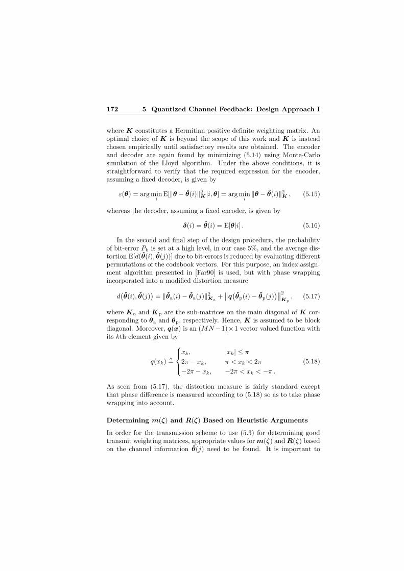
172 5 Quantized Channel Feedback: Design Approach I
where K constitutes a Hermitian positive definite weighting matrix. Anoptimal choice of K is beyond the scope of this work and K is insteadchosen empirically until satisfactory results are obtained. The encoderand decoder are again found by minimizing (5.14) using Monte-Carlosimulation of the Lloyd algorithm. Under the above conditions, it isstraightforward to verify that the required expression for the encoder,assuming a fixed decoder, is given by
ε(θ) = arg mini
E[‖θ − θ(i)‖2K |i,θ] = arg min
i‖θ − θ(i)‖2
K , (5.15)
whereas the decoder, assuming a fixed encoder, is given by
δ(i) = θ(i) = E[θ|i] . (5.16)
In the second and final step of the design procedure, the probabilityof bit-error Pb is set at a high level, in our case 5%, and the average dis-tortion E[d(θ(i), θ(j))] due to bit-errors is reduced by evaluating differentpermutations of the codebook vectors. For this purpose, an index assign-ment algorithm presented in [Far90] is used, but with phase wrappingincorporated into a modified distortion measure
d(θ(i), θ(j)
)= ‖θa(i) − θa(j)‖2
Ka+∥∥q(θp(i) − θp(j)
)∥∥
2
Kp, (5.17)
where Ka and Kp are the sub-matrices on the main diagonal of K cor-responding to θa and θp, respectively. Hence, K is assumed to be blockdiagonal. Moreover, q(x) is an (MN −1)×1 vector valued function withits kth element given by
q(xk) ,
xk, |xk| ≤ π
2π − xk, π < xk < 2π
−2π − xk, −2π < xk < −π .
(5.18)
As seen from (5.17), the distortion measure is fairly standard exceptthat phase difference is measured according to (5.18) so as to take phasewrapping into account.
Determining m(ζ) and R(ζ) Based on Heuristic Arguments
In order for the transmission scheme to use (5.3) for determining goodtransmit weighting matrices, appropriate values for m(ζ) and R(ζ) basedon the channel information θ(j) need to be found. It is important to
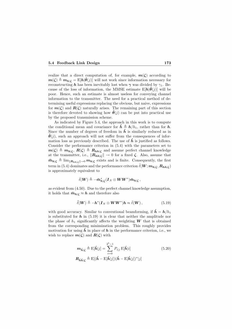
5.4 Feedback Link Design 173
realize that a direct computation of, for example, m(ζ) according tom(ζ) , mh|ζ = E[h|θ(j)] will not work since information necessary forreconstructing h has been inevitably lost when γ was divided by γ1. Be-cause of the loss of information, the MMSE estimate E[h|θ(j)] will bepoor. Hence, such an estimate is almost useless for conveying channelinformation to the transmitter. The need for a practical method of de-termining useful expressions replacing the obvious, but naive, expressionsfor m(ζ) and R(ζ) naturally arises. The remaining part of this sectionis therefore devoted to showing how θ(j) can be put into practical useby the proposed transmission scheme.
As indicated by Figure 5.4, the approach in this work is to computethe conditional mean and covariance for h , h/h1, rather than for h.Since the number of degrees of freedom in h is similarly reduced as inθ(j), such an approach will not suffer from the consequences of infor-mation loss as previously described. The use of h is justified as follows.Consider the performance criterion in (5.4) with the parameters set tom(ζ) , mh|ζ , R(ζ) , Rhh|ζ and assume perfect channel knowledgeat the transmitter, i.e., ‖Rhh|ζ‖ → 0 for a fixed ζ. Also, assume that
mh|ζ , lim‖Rhh|ζ‖→0 mh|ζ exists and is finite. Consequently, the first
term in (5.4) dominates and the performance criterion ˜(W ;mh|ζ ,Rhh|ζ)is approximately equivalent to
¯(W ) , −m∗h|ζ(IN ⊗ WW ∗)mh|ζ ,
as evident from (4.50). Due to the perfect channel knowledge assumption,it holds that mh|ζ ≈ h and therefore also
¯(W ) , −h∗(IN ⊗ WW ∗)h ≈ ¯(W ) , (5.19)
with good accuracy. Similar to conventional beamforming, if h = h/h1
is substituted for h in (5.19) it is clear that neither the amplitude northe phase of h1 significantly affects the weighting W that is obtainedfrom the corresponding minimization problem. This roughly providesmotivation for using h in place of h in the performance criterion, i.e., wewish to replace m(ζ) and R(ζ) with
mh|ζ , E[h|j] =
2b−1∑
i=0
Pi|j E[h|i] (5.20)
Rhh|ζ , E[(h − E[h|j])(h − E[h|j])∗|j]

174 5 Quantized Channel Feedback: Design Approach I
= E[hh∗|j] − E[h|j] E[h|j]∗
=
2b−1∑
i=0
Pi|j E[hh∗|i] − mh|ζm∗
h|ζ, (5.21)
respectively. However, these asymptotically motivated entities need to beslightly modified before they can be successfully used in scenarios wherethe channel knowledge is not perfect. Specifically, three issues need to beaddressed:
1. To approximately keep the original proportion between the first andsecond term in the performance criterion (5.4), the lost amplitudeinformation is partially compensated for by multiplying h with themean E[|h1|].
2. Since h1 ≡ 1, element (1, 1) of Rhh|ζ will be zero, which means thatRhh|ζ is singular. A reasonable fix for this problem is to set element
(1, 1) to the average variance of the other elements. In other words,the element is set to tr(Rhh|ζ)/(MN − 1), where Rhh|ζ represents
the (MN − 1) × (MN − 1) lower right block of Rhh|ζ and h is
defined through h =[
1 hT]T
. This modification makes intuitive
sense since it means that Rhh|ζ can be viewed as a parameter whichseamlessly tunes between conventional beamforming and OSTBC.
3. The use of (5.20), (5.21) and the two previous modifications in con-junction with the transmission scheme generally gives good perfor-mance. However, simulation results indicate that the transmissionscheme overcompensates for large quantization errors and therebysteers the weighting W too close toward an open-loop solution.Conventional beamforming is on the other hand relatively robustagainst pure quantization errors and provides acceptable perfor-mance for such scenarios. In cases where only quantization errorsaffect the quality of the channel information, the performance ofweighted OSTBC can be improved by making the conditional co-variance small, since the transmission scheme then resembles clas-sical beamforming and thus inherits its for this case good perfor-mance. It is of course highly desirable if such a modification alsoworks well when other errors influence the channel information. Asis shown next, both these latter aspects are taken into account by

5.5 Detecting the Transmit Weighting 175
removing a part of the conditional covariance that can be consid-ered to be due to quantization errors.
Recall the result in (5.9) that Rhh|ζ , assuming a feedback link oftype I, can be decomposed into three terms. One of the terms maybe attributed to quantization errors. Obviously, the assumptionsused when deriving that result do not hold in the present case. Nev-ertheless, (5.9) is still reasonable for the feedback link type underconsideration so inspired by the expression for the term in (5.9)that corresponds to quantization errors, we take
R(q)
hh|ζ, RhγR−1
γγ E[(γ − E[γ|i])(γ − E[γ|i])∗|j]R−1γγR∗
hγ
= RhγR−1γγ(E[γγ∗|j] −
2b−1∑
i=0
Pi|j E[γ|i] E[γ|i]∗)R−1γγR∗
hγ(5.22)
as a measure of the contribution of the quantization distortion toRhh|ζ . Motivated by the above discussion, Rhh|ζ is replaced with
R(f+c)
hh|ζ, Rhh|ζ −R
(q)
hh|ζ. Examining simulation results shows that
this pragmatic approach works well and improves the performancein scenarios with coarsely quantized channel information.
Thus, to summarize, incorporating the three heuristic modificationsmentioned above into the system means that the parameters passed tothe transmission scheme are set to
m(ζ) , E[|h1|]mh|ζ
R(ζ) , E[|h1|]2
tr(R
(f+c)
hh|ζ
)/(MN − 1) 0T
0 R(f+c)
hh|ζ
.
Because R(f+c)
hh|ζis computed as a difference between two matrices, R
(f+c)
hh|ζ
and hence Rhh|ζ is not necessarily positive definite. This problem isavoided by setting negative eigenvalues of Rhh|ζ to zero and adding asmall regularizing term εIMN , ε > 0 to the resulting matrix.
5.5 Detecting the Transmit Weighting
For high performance it is desirable to use coherent ML detection at thereceiver. To implement such a scheme, the transmit weighting must be

176 5 Quantized Channel Feedback: Design Approach I
known at the receiver. Because b-bit quantization is assumed, the trans-
mitter may have used any out of the 2b different weights W (δ(j))2b−1j=0 .
Knowing which one is not a problem as long as the feedback link is freefrom bit-errors, since then j = i and the receiver can demodulate usingW (δ(i)). However, in the presence of bit-errors, i does not necessarilyequal j and hence the receiver can no longer be sure that W (δ(i)) wasused in the transmission. To mitigate this problem, it is shown nexthow the receiver can detect the value of j, based on knowledge of i, thereceived signal and a training sequence.
In the derivation to follow, it is assumed that the transmitted signalcan be divided into frames, where each frame contains a block of unknownOSTB codewords, corresponding to the data of interest, and possiblyalso a known training sequence. Recall from the system model that thechannel is assumed known and constant for the duration of a frame. Bygrouping, similarly to as in (5.1), a block of received signal vectors x(n)into a matrix Xt+d, the received signal for one such frame can be writtenon the form
Xt+d = H∗W (δ(j))Ct+d + Et+d ,
where
Ct+d =[Ct Cd
]
consists of a training part Ct and a data part Cd of unknown codewordsand where Xt+d and Et+d are similarly defined. The lengths of thetraining and the data sequence are denoted Lt and Ld, respectively.
Based on knowledge of i and Xt+d, the feedback channel output j isdetected possibly jointly with the data Cd according to the maximum aposteriori decision rule, i.e.,
j, ˆCd = arg maxj,Cd
p(j, Cd|i,Xt+d)
= arg maxj,Cd
p(Xt+d|i, j, Cd)p(j, Cd|i)p(Xt+d|i)
= arg maxj,Cd
p(Xt+d|j, Cd)p(j|i)p(Cd)
= arg maxj,Cd
p(Xt|j)p(Xd|j, Cd)Pj|i
= arg minj,Cd
(‖Xt − H∗W (δ(j))Ct‖2
F + ‖Xd − H∗W (δ(j))Cd‖2F
− σ2 log(Pj|i)), (5.23)

5.6 Numerical Examples 177
where p(u|v) denotes the probability mass/density function of u condi-tioned on v, p(j, Cd|i) = p(j|i, Cd)p(Cd|i) = p(j|i)p(Cd) is due to theassumption that the output Cd of the OSTB encoder only depends onthe data to be transmitted and is statistically independent of all otherrandom quantities and where the fourth equality follows from discard-ing parameter independent factors, the whiteness of the noise and theuniform distribution of Cd. The receiver’s knowledge about i is ob-viously incorporated into the detection process through the last term,which guarantees that j = j = i is obtained in the absence of bit-errors.
It is evident from (5.23) that compared with when the transmitweighting is known, the computational complexity in the general case ofjoint detection increases a factor of 2b since there are 2b different transmitweights to be tried. Fortunately, the complexity is far from being as highas when performing an exhaustive search, since for each tentative j thedetection of the OSTB code can be efficiently implemented by decodingthe constituent information symbols separately as in (3.14).
Nevertheless, such joint detection may still be prohibitively expensivein some cases, making it worthwhile to consider the special case whenLd = 0, i.e., the second term in (5.23) is omitted and the detectionof the transmit weighting is based on the training part alone. Once thetransmit weighting has been established, the data sequence can thereafterbe detected as in (3.14), thus avoiding joint detection. Naturally, therequirements on the length of the training sequence might be tougher inthis case, compared with when joint detection is used.
Note that the training sequence Ct is used for the sole purpose ofdetecting W . This together with the previously mentioned assumptionthat the channel matrix H is known at the receiver typically means thatH needs to be estimated from another training sequence which is notweighted by W . In practice, such a training sequence may be transmittedbefore or after Ct or, as in the WCDMA system [3GP02b], in parallel ona so-called common pilot channel.
5.6 Numerical Examples
In order to illustrate the benefits of the proposed transmission schemes,simulations based on the simplified fading scenario described in Section5.2.2 were performed. The focus is on a system with two transmit anten-nas and one receive antenna. Two bit quantization in conjunction witha type II feedback link was evaluated for all simulation cases to show
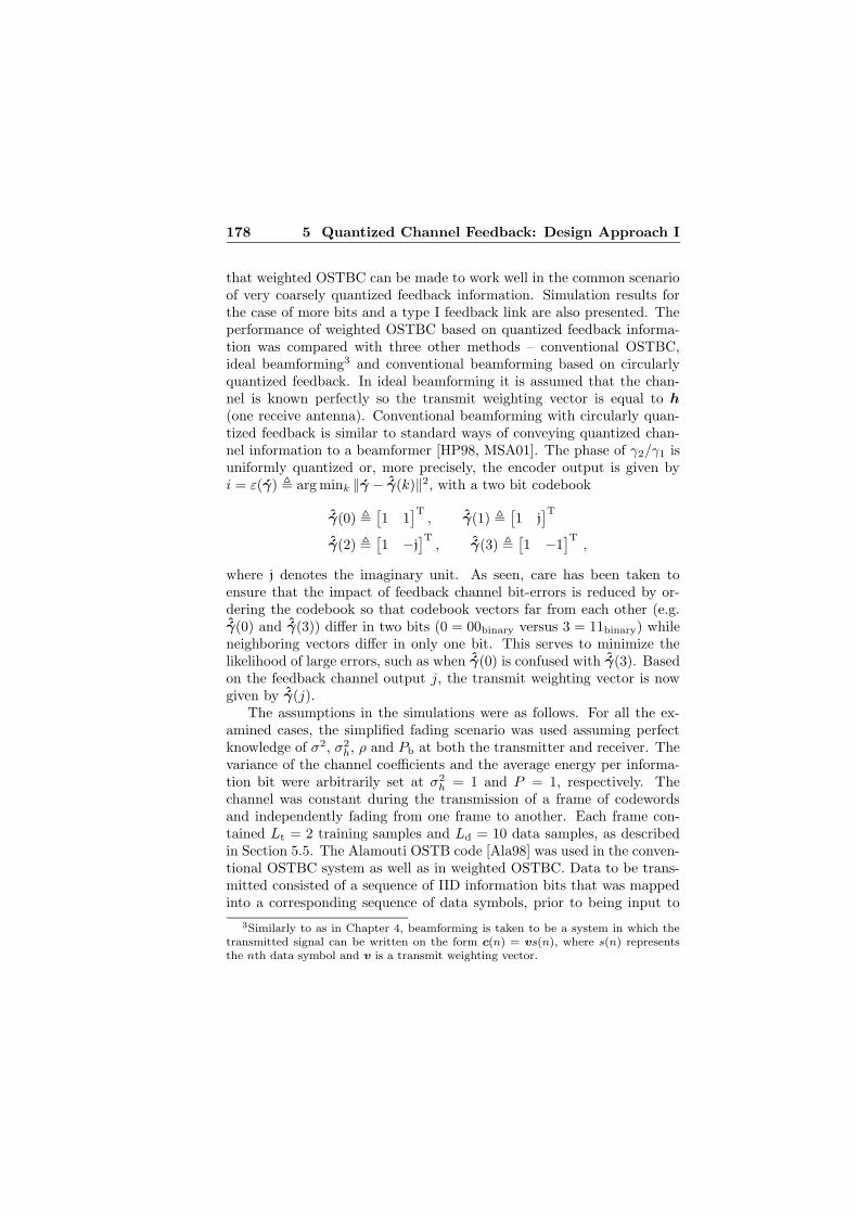
178 5 Quantized Channel Feedback: Design Approach I
that weighted OSTBC can be made to work well in the common scenarioof very coarsely quantized feedback information. Simulation results forthe case of more bits and a type I feedback link are also presented. Theperformance of weighted OSTBC based on quantized feedback informa-tion was compared with three other methods – conventional OSTBC,ideal beamforming3 and conventional beamforming based on circularlyquantized feedback. In ideal beamforming it is assumed that the chan-nel is known perfectly so the transmit weighting vector is equal to h
(one receive antenna). Conventional beamforming with circularly quan-tized feedback is similar to standard ways of conveying quantized chan-nel information to a beamformer [HP98, MSA01]. The phase of γ2/γ1 isuniformly quantized or, more precisely, the encoder output is given byi = ε(γ) , arg mink ‖γ − ˆγ(k)‖2, with a two bit codebook
ˆγ(0) ,[1 1
]T, ˆγ(1) ,
[1 j
]T
ˆγ(2) ,[1 −j
]T, ˆγ(3) ,
[1 −1
]T,
where j denotes the imaginary unit. As seen, care has been taken toensure that the impact of feedback channel bit-errors is reduced by or-dering the codebook so that codebook vectors far from each other (e.g.ˆγ(0) and ˆγ(3)) differ in two bits (0 = 00binary versus 3 = 11binary) whileneighboring vectors differ in only one bit. This serves to minimize thelikelihood of large errors, such as when ˆγ(0) is confused with ˆγ(3). Basedon the feedback channel output j, the transmit weighting vector is nowgiven by ˆγ(j).
The assumptions in the simulations were as follows. For all the ex-amined cases, the simplified fading scenario was used assuming perfectknowledge of σ2, σ2
h, ρ and Pb at both the transmitter and receiver. Thevariance of the channel coefficients and the average energy per informa-tion bit were arbitrarily set at σ2
h = 1 and P = 1, respectively. Thechannel was constant during the transmission of a frame of codewordsand independently fading from one frame to another. Each frame con-tained Lt = 2 training samples and Ld = 10 data samples, as describedin Section 5.5. The Alamouti OSTB code [Ala98] was used in the conven-tional OSTBC system as well as in weighted OSTBC. Data to be trans-mitted consisted of a sequence of IID information bits that was mappedinto a corresponding sequence of data symbols, prior to being input to
3Similarly to as in Chapter 4, beamforming is taken to be a system in which thetransmitted signal can be written on the form c(n) = vs(n), where s(n) representsthe nth data symbol and v is a transmit weighting vector.

5.6 Numerical Examples 179
the OSTB encoder. Each data symbol was taken from a gray coded,four quadrature phase shift keying (4-QPSK), signal constellation. Thetype II feedback links were designed using a diagonal weighting matrixK = diag(0.2, 0.8). This choice was found empirically and emphasizesthe importance of primarily conveying phase information. Throughoutthe simulations, BER was used as the performance measure. The SNRwas measured for the system using conventional OSTBC and defined as
SNR ,E[‖H∗C‖2
F]
LNσ2,
where C =√
Po/MC represents the transmitted signals. The expressionfor the SNR is equal to the total received average signal energy, dividedby the total average noise energy.
Varying the SNR
In Figure 5.5, the BER as a function of the SNR is plotted. Only quan-tization errors impair the quality of the channel information. Hence,ρ → 1 and Pb = 0, where the latter implies that the receiver automati-cally knows which transmit weighting that was used.
Using two bit quantization and a type II feedback link, the perfor-mance of weighted OSTBC is seen to be similar to the performance ofconventional beamforming. As the number of bits is increased, the perfor-mance quickly approaches that of ideal beamforming. On the other hand,the performance of weighted OSTBC based on a type I feedback link issignificantly poorer for the two bit case. There are simply not enoughbits to capture any useful channel information. Because weighted OS-TBC takes the quality of the channel information into account, the per-formance is however not worse than conventional OSTBC. As expectedand illustrated by the eight bit curves, the difference between a type I andtype II feedback link becomes smaller as the number of bits increases. Itis also seen that weighted OSTBC is essentially robust against quantiza-tion errors in the sense that the performance is better than conventionalOSTBC (with the minor exception of type I eight bit weighted OSTBC athigh SNR values). Conventional beamforming with circular quantizationis clearly better than a type I system at handling quantization errors.
Robustness against errors in the initial channel information is demon-strated in Figure 5.6. The assumption of ρ = 0.1 means that the qualityof the channel knowledge is poor, even though Pb = 0. The curves corre-sponding to weighted OSTBC are seen to closely follow the conventional

180 5 Quantized Channel Feedback: Design Approach I
−5 0 5 10 15 20 2510−5
10−4
10−3
10−2
10−1
100
Conv. OSTBCWeighted OSTBC: Type I, 2 bitsWeighted OSTBC: Type II, 2 bitsConv. beamforming: circular quant., 2 bitsWeighted OSTBC: Type I, 8 bitsWeighted OSTBC: Type II, 8 bitsIdeal beamforming
PSfrag replacements
SNR [dB]
BE
R
Figure 5.5: Demonstrates how quantization errors affect the perfor-mance. Simplified fading scenario with ρ → 1, M = 2 transmit antennas,N = 1 receive antenna and Pb = 0.
OSTBC curve while conventional beamforming is not robust since theperformance rapidly deteriorates as the SNR is increased.
Next, the behavior of the proposed transmission scheme in the pres-ence of feedback channel bit-errors is illustrated in Figures 5.7 and 5.8.The feedback channel BER is set to Pb = 0.4 and results for both whenthe receiver knows and does not know the weighting matrix W are plot-ted. For the latter case, the weighting matrix was detected according to(5.23). The same detection method was also used for the beamformingcase but now with Cd representing a symbol sequence instead of space-time codewords. Again, weighted OSTBC is robust while conventionalbeamforming is unable to handle the situation.

5.6 Numerical Examples 181
−5 0 5 10 15 20 2510−5
10−4
10−3
10−2
10−1
100
Conv. OSTBCWeighted OSTBC: Type I, 8 bitsWeighted OSTBC: Type II, 2 bitsConv. beamforming: circular quant., 2 bitsIdeal beamforming
PSfrag replacements
SNR [dB]
BE
R
Figure 5.6: Impact of non-perfect initial channel information. Simpli-fied fading scenario with ρ = 0.1, M = 2 transmit antennas, N = 1receive antenna and Pb = 0.
Varying the BER of the Feedback Channel
To further illustrate the robustness against bit-errors introduced by thefeedback channel, the corresponding BER Pb was varied while the SNRwas held fixed at 15 dB. Results corresponding to when the receiverknows as well as does not know the weighting matrix are presented inFigures 5.9 and 5.10, respectively.
As expected, conventional beamforming is seen to perform poorlywhen Pb is large. Weighted OSTBC for known W , on the other hand,approaches conventional OSTBC in performance as Pb is increased. Onlya modest deterioration is incurred for the type II system when the receiverhas to detect the transmit weighting matrix. The type I system suffersmore because of higher failure rate in the detection process due to thelarge number of possible transmit weights to choose from. From these
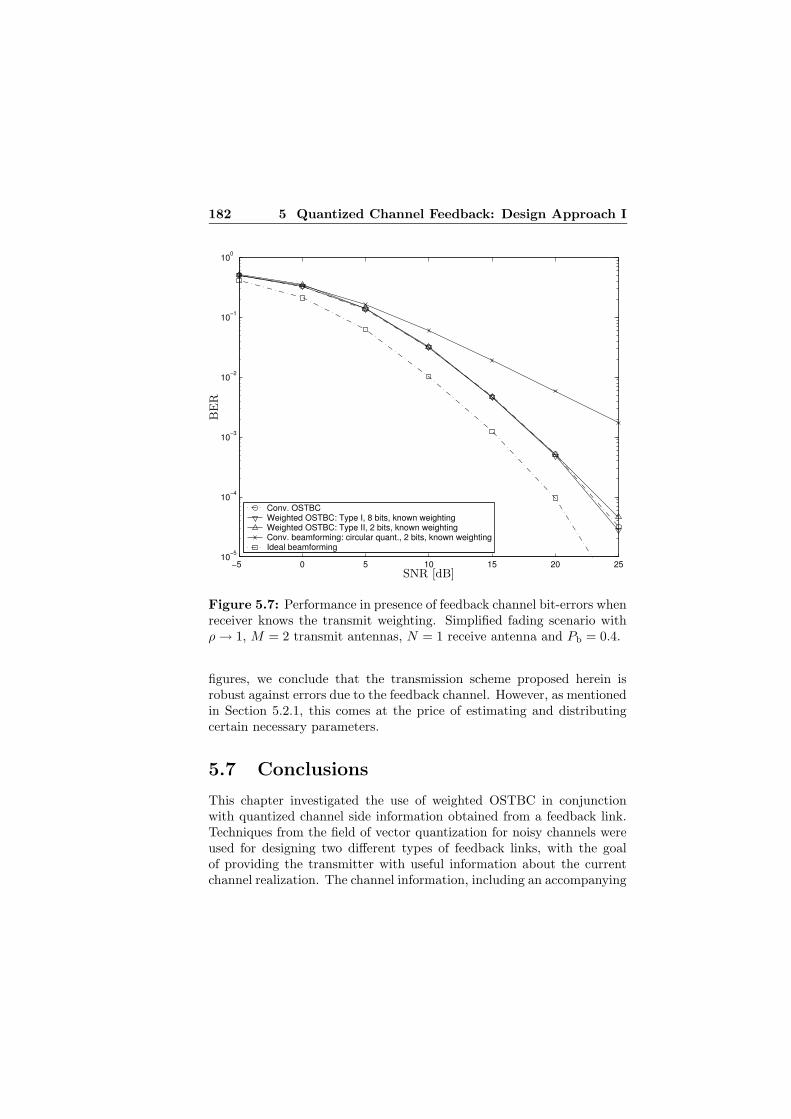
182 5 Quantized Channel Feedback: Design Approach I
−5 0 5 10 15 20 2510−5
10−4
10−3
10−2
10−1
100
Conv. OSTBCWeighted OSTBC: Type I, 8 bits, known weightingWeighted OSTBC: Type II, 2 bits, known weightingConv. beamforming: circular quant., 2 bits, known weightingIdeal beamforming
PSfrag replacements
SNR [dB]
BE
R
Figure 5.7: Performance in presence of feedback channel bit-errors whenreceiver knows the transmit weighting. Simplified fading scenario withρ → 1, M = 2 transmit antennas, N = 1 receive antenna and Pb = 0.4.
figures, we conclude that the transmission scheme proposed herein isrobust against errors due to the feedback channel. However, as mentionedin Section 5.2.1, this comes at the price of estimating and distributingcertain necessary parameters.
5.7 Conclusions
This chapter investigated the use of weighted OSTBC in conjunctionwith quantized channel side information obtained from a feedback link.Techniques from the field of vector quantization for noisy channels wereused for designing two different types of feedback links, with the goalof providing the transmitter with useful information about the currentchannel realization. The channel information, including an accompanying

5.7 Conclusions 183
−5 0 5 10 15 20 2510−5
10−4
10−3
10−2
10−1
100
Conv. OSTBCWeighted OSTBC: Type I, 8 bits, unknown weightingWeighted OSTBC: Type II, 2 bits, unknown weightingConv. beamforming: circular quant., 2 bits, unknown weightingIdeal beamforming
PSfrag replacements
SNR [dB]
BE
R
Figure 5.8: Performance in presence of feedback channel bit-errors whenreceiver has to detect the transmit weighting. Simplified fading scenariowith ρ → 1, M = 2 transmit antennas, N = 1 receive antenna andPb = 0.4.
reliability measure, was then used for determining a suitable codebook oftransmit weighting matrices. The resulting transmission scheme providesa seamless combination of conventional beamforming and OSTB coding,robust against errors in the channel side information due to feedbackdelay, quantization as well as feedback channel bit-errors. Numericalexamples provided support of this claim.

184 5 Quantized Channel Feedback: Design Approach I
10−4 10−3 10−2 10−1 10010−3
10−2
10−1
Conv. OSTBCWeighted OSTBC: Type I, 8 bits, known weightingWeighted OSTBC: Type II, 2 bits, known weightingConv. beamforming: circular quant., 2 bits, known weighting
PSfrag replacements
Pb
BE
R
Figure 5.9: Performance in the presence of feedback channel bit-errorswhen the receiver knows the transmit weighting. Simplified fading sce-nario with ρ → 1, M = 2 transmit antennas, N = 1 receive antenna andSNR = 15 dB.

5.7 Conclusions 185
10−4 10−3 10−2 10−1 10010−3
10−2
10−1
Conv. OSTBCWeighted OSTBC: Type I, 8 bits, unknown weightingWeighted OSTBC: Type II, 2 bits, unknown weightingConv. beamforming: circular quant., 2 bits, unknown weighting
PSfrag replacements
Pb
BE
R
Figure 5.10: Performance in the presence of feedback channel bit-errorswhen the receiver has to detect the transmit weighting. Simplified fadingscenario with ρ → 1, M = 2 transmit antennas, N = 1 receive antennaand SNR = 15 dB.

186 5 Quantized Channel Feedback: Design Approach I
Appendix 5.A Conditional Covariance for
Feedback Link Type I
The conditional covariance Rhh|ζ for feedback link type I is given by
Rhh|ζ = E[hh∗|j] − E[h|j] E[h|j]∗ . (5.24)
Recall that h|γ is independent of j. The first term in (5.24) is rewrittenas
E[hh∗|j] = E[E[hh∗|γ, j]
∣∣j]
= E[Rhh|γ + mh|γm∗h|γ |j]
= Rhh|γ
+ E[(
mh + RhγR−1γγ(γ − mγ)
)(mh + RhγR−1
γγ(γ − mγ))∗∣∣j]
= Rhh|γ + mhm∗h + mh E[γ − mγ |j]∗R−1
γγR∗hγ
+RhγR−1γγ E[γ−mγ |j]m∗
h+RhγR−1γγ E[(γ−mγ)(γ−mγ)∗|j]R−1
γγR∗hγ ,
where the third equality follows from the fact that Rhh|γ = Rhh −RhγR−1
γγR∗hγ is independent of γ and hence of j. The second term in
(5.24) is expressed as
E[h|j] E[h|j]∗ = E[E[h|γ, j]
∣∣j]E[E[h|γ, j]
∣∣j]∗
= E[mh + RhγR−1γγ(γ − mγ)|j] E[mh + RhγR−1
γγ(γ − mγ)|j]∗
= mhm∗h + mh E[γ − mγ |j]∗R−1
γγR∗hγ + RhγR−1
γγ E[γ − mγ |j]m∗h
+ RhγR−1γγ E[γ − mγ |j] E[γ − mγ |j]∗R−1
γγR∗hγ .
Hence, combining the first and second term, gives the conditional covari-ance
Rhh|ζ = Rhh|γ
+RhγR−1γγ
(E[(γ−mγ)(γ−mγ)∗|j]−E[γ−mγ |j] E[γ−mγ |j]∗
)R−1
γγR∗hγ
= Rhh|γ
+RhγR−1γγ E
[(γ−mγ−E[γ−mγ |j])(γ−mγ−E[γ−mγ |j])∗
∣∣j]R−1
γγR∗hγ
= Rhh|γ
+ RhγR−1γγ E
[(γ − E[γ|j])(γ − E[γ|j])∗
∣∣j]R−1
γγR∗hγ
= Rhh|γ + RhγR−1γγ(E[γγ∗|j] − E[γ|j] E[γ|j]∗)R−1
γγR∗hγ . (5.25)

5.A Conditional Covariance for Feedback Link Type I 187
5.A.1 Decomposing the Conditional Covariance intoThree Terms
Consider
Rhh|ζ = Rhh|γ + RhγR−1γγ E
[(γ − E[γ|j])(γ − E[γ|j])∗
∣∣j]R−1
γγR∗hγ .
in (5.25). Expanding E[(γ − E[γ|j])(γ − E[γ|j])∗
∣∣j]
by utilizing thatγ − E[γ|j] = γ − E[γ|i] − (E[γ|j] − E[γ|i]) gives
E[(γ − E[γ|j])(γ − E[γ|j])∗
∣∣j]
= E[(γ−E[γ|i])(γ−E[γ|i])∗
∣∣j]+E
[(E[γ|j]−E[γ|i])(E[γ|j]−E[γ|i])∗
∣∣j]
−E[(E[γ|j]−E[γ|i])(γ−E[γ|i])∗
∣∣j]−E
[(γ−E[γ|i])(E[γ|j]−E[γ|i])∗
∣∣j].
It is clear that the two last terms are zero since
E[(E[γ|j] − E[γ|i])(γ − E[γ|i])∗
∣∣j]
= E[
E[(E[γ|j] − E[γ|i])(γ − E[γ|i])∗
∣∣i, j
]∣∣∣j]
= E[(E[γ|j] − E[γ|i])(E[γ|i] − E[γ|i])∗
∣∣j]
= 0 .
Hence,
E[(γ − E[γ|j])(γ − E[γ|j])∗
∣∣j]
= E[(γ − E[γ|i])(γ − E[γ|i])∗
∣∣j]
+ E[(E[γ|j] − E[γ|i])(E[γ|j] − E[γ|i])∗
∣∣j]
and thus,
Rhh|ζ = Rhh|γ + RhγR−1γγ E
[(γ − E[γ|i])(γ − E[γ|i])∗
∣∣j]R−1
γγR∗hγ
+ RhγR−1γγ E
[(E[γ|j] − E[γ|i])(E[γ|j] − E[γ|i])∗
∣∣j]R−1
γγR∗hγ .


Chapter 6
Quantized ChannelFeedback: DesignApproach II
Also this chapter considers a wireless MIMO communication system inwhich the transmitter has access to quantized channel side informationobtained from a feedback link. The setup is thus similar to the scenarioconsidered in the previous chapter. This time however, a new space-timecode performance criterion is derived that is specifically tailored to quan-tized channel side information. The performance criterion is similar instructure to the one used earlier and can hence be utilized for construct-ing any of the three code types described in the thesis. Still, the focus inthe present chapter is mostly on unstructured codes.
Because the effects of quantization are taken into account alreadyat the outset when deriving the performance criterion, heuristic modi-fications of the code design procedure in order to obtain good perfor-mance are not needed. This is in contrast to the methods in Chapter 5.Compared with that chapter, the development to follow thus constitutesa mathematically cleaner approach for incorporating quantized channelside information into the design of space-time codes.
Efficient unstructured codes are found by utilizing a gradient searchtechnique for minimizing the performance criterion. Properties of op-timal unstructured codes are derived for a number of different cases.Design procedures for linear dispersive codes and weighted OSTBC are

190 6 Quantized Channel Feedback: Design Approach II
briefly described and implemented. Unstructured codes designed usingthe techniques developed in this work are shown to perform better thancomparable OSTB codes, even without channel knowledge at the trans-mitter. Experimental investigations reveal that the design procedure forlinear dispersive codes appears to automatically produce OSTB codes inthe case of no channel knowledge.
Simulation results for a spatially uncorrelated flat Rayleigh fadingscenario using two and four transmit antennas and one receive antennademonstrate that the designed unstructured codes give significant gainsrelative conventional transmission schemes. In addition, the impact onperformance due to the choice of code type is illustrated by means ofone representative simulation example. The unstructured code is seen toperform significantly better than both weighted OSTBC and the lineardispersive code. It is also noted that the two latter have similar perfor-mance.
6.1 Introduction
In general, conventional space-time codes [GFBK99, TSC98, TJC99] havebeen designed for situations where the transmitter has no knowledgeabout the wireless MIMO/MISO channel. The present work, on theother hand, considers the design of space-time block codes that may uti-lize channel information at the transmitter, if available, for increasingthe performance. Just as in Chapter 5, the design is targeted towardsa non-power-controlled narrowband scenario in which the transmitter isprovided with quantized channel information from the receiver via a ded-icated feedback link. While the receiver has perfect channel knowledge,both quantization errors as well as feedback delay are assumed to plaguethe channel information at the transmitter. A model describing thesedetrimental effects is exploited in the code design. In this way, the con-structed codes continue to work well even if the quality of the channelinformation is poor.
The channel knowledge is incorporated into the code constructionprocess by utilizing a new design criterion that is developed specificallyto deal with scenarios in which the channel side information is quantized.The design criterion is similar in structure to the one originally presentedin Chapter 4, making it straightforward to modify the code design pro-cedures described therein so that they utilize the new design criterion.Most of the work is focused on the design and analysis of unstructured

6.1 Introduction 191
space-time block codes. However some effort is also spent on the designof linear dispersive codes and weighted OSTBC.
Related work includes the design of conventional space-time codes[GFBK99, TSC98, BBH00, ARU01, MBV02, HH02b], the design of mod-ulation signal sets [FGW74, HSN91] and how to utilize non-perfect chan-nel information at the transmitter [Wit95, NLTW98, HP98], respectively.
In [GFBK99, TSC98], code design criteria were introduced and usedfor manually constructing conventional space-time codes exhibiting a highdegree of structure. The design criterion derived and used in this chap-ter constitutes a generalization of these criteria so as to handle also thecase of (non-perfect) channel knowledge. A more automated design pro-cess was investigated in [BBH00], where an exhaustive search techniquewas employed in order to find appropriate space-time trellis codes. In[ARU01, MBV02] the code search was conducted over the set of unitarycodeword matrices to produce codes suitable for a non-coherent detectionscenario in which the channel is unknown at the receiver. Linear disper-sive codes were designed in [HH02b] based on maximizing an informationtheoretic capacity measure. The design of efficient signal constellationsand modulation signal sets for a SISO channel was treated in [FGW74]and [HSN91], respectively. Inspired by the numerical search approach inthe two latter papers, the present work applies gradient search techniquesfor minimizing the design criterion and hence obtaining suitable channelside information dependent space-time block codes.
The present work contributes in several ways. A major contribu-tion is the development of a new design criterion that specifically handlesquantized channel side information. The design criterion lays the founda-tion of a general strategy for incorporating non-perfect quantized channelside information into the design of space-time codes. Another importantcontribution is the development of design procedures for realizing thisstrategy in the cases of unstructured and linear dispersive codes as wellas for weighted OSTBC. The focus is however on unstructured codes forwhich a theoretical analysis is provided that illustrates the intuitivelypleasing characteristics of the resulting transmission scheme and givesuseful insights into the problem. Due to the unstructured nature of thecodewords, these codes potentially have better performance than all othercorresponding block codes with structure, albeit at the cost of a higherdecoding complexity. Hence an additional field of application for ourunstructured code design method is to produce benchmark codes thatquantify the loss in performance that results from introducing structureto reduce decoding complexity. This is illustrated herein by simulation

192 6 Quantized Channel Feedback: Design Approach II
examples and coding gain measurements showing that the unstructuredcodes perform better than comparable OSTB codes. Such gains are ob-tained even when no channel information is available. A particularlyfascinating result is that the design procedure for linear dispersive codesseems to, in the case of no channel knowledge, automatically produceOSTB codes, if such codes exist for the setup under consideration. Fi-nally, it should be noted that the design methods presented herein areeasily extended to also cope with errors in the channel side informationdue to bit-errors introduced by the feedback channel.
The remaining part of the chapter is organized as follows. In Sec-tion 6.2, the generic system model is briefly reviewed and additionalassumptions and preliminaries are described. The design criterion isderived in Section 6.3 and utilized for defining a design procedure forunstructured codes in terms of an optimization problem. The designof linear dispersive codes and weighed OSTBC is also addressed. Vari-ous properties of optimal unstructured codes are derived in Section 6.4.The numerical technique used for solving the optimization problem isdescribed in Section 6.5. Section 6.6 gives explicit examples of designedcodes of the unstructured type and discusses properties of several othercodes, including a couple of constructed linear dispersive codes. Finally,the performance of some constructed codes is assessed by means of sim-ulation of a spatially uncorrelated flat Rayleigh fading scenario and theresults are presented in Section 6.7.
6.2 System Model
This work considers a MIMO wireless communication system making useof space-time block codes that utilize quantized channel side informationat the transmitter for enhancing the performance. The channel side in-formation is obtained from the receiver via a dedicated feedback link.The generic system model and the assumptions regarding code struc-tures described in Chapter 3 apply, as indicated by the setup illustratedin Figure 6.1.
The channel side information ζ now comes in the form of an integeri representing the quantized output of the feedback link. Hence, thechannel code C = C(i) currently in use is determined out of a set C(i) ofspace-time block codes. Codes of the types unstructured, linear dispersiveor weighted OSTBC may be used. These code types are discussed indetail in Section 3.2. The focus in this work is however primarily on

6.2 System Model 193
PSfrag replacements
......
Space-Time
Encoder
W
M N
c(n) x(n)Receiver
...
H ⇔ h=vec(H)︷ ︸︸ ︷
⇑
i
C = C(i) γ
C(i) Enc: ε(γ)
Figure 6.1: System model.
unstructured codes. Hence, the codes in C(i) are henceforth assumed tobe unstructured, unless explicitly stated otherwise. Each code in C(i)will be designed so as to adapt the code to the specific channel knowledge,as described by the corresponding value of i. The resulting informationcarrying signals are transmitted over a wireless frequency-nonselectivefading channel, picked up by the antennas at the receiver and thereafterdecoded to produce an estimate of the transmitted message.
Recall from the generic system model that there are M transmit andN receive antennas and that the received signal vectors x(n) = H∗c(n)+e(n) during the time interval n = 0, 1, · · · , L−1 are grouped into a matrixX given by
X = H∗C + E , (6.1)
where the zero-mean IID complex Gaussian elements of the noise matrixE have variance σ2. Here, the MIMO channel is described by the M ×Nmatrix H or its vectorized counterpart h , vec(H) with elements hk.The transmitted codeword C belongs to the current choice C , CkK
k=1
of channel code. The rate of the code is log2(K)/L information bits perchannel use. The receiver is assumed to know the channel perfectly andrecovers the transmitted codeword by means of ML decoding accordingto
C = arg minC∈C(i)
‖X − H∗C‖2F , (6.2)
where C represents the estimated codeword.
The output power is limited in the same manner as previously. Hence,conditioned on the use of a certain code C(i), it is assumed that thetransmission is such that all the codewords are equally probable and that
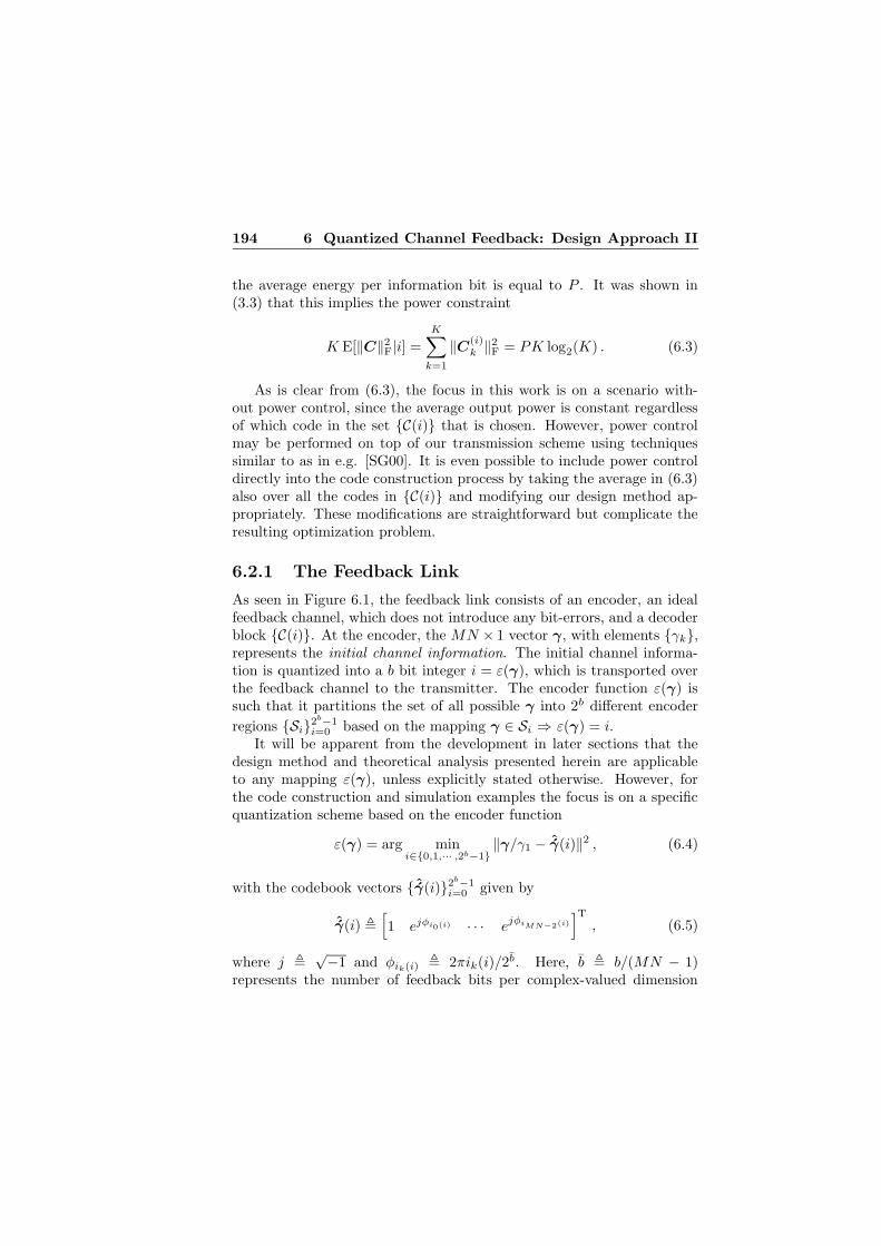
194 6 Quantized Channel Feedback: Design Approach II
the average energy per information bit is equal to P . It was shown in(3.3) that this implies the power constraint
K E[‖C‖2F|i] =
K∑
k=1
‖C(i)k ‖2
F = PK log2(K) . (6.3)
As is clear from (6.3), the focus in this work is on a scenario with-out power control, since the average output power is constant regardlessof which code in the set C(i) that is chosen. However, power controlmay be performed on top of our transmission scheme using techniquessimilar to as in e.g. [SG00]. It is even possible to include power controldirectly into the code construction process by taking the average in (6.3)also over all the codes in C(i) and modifying our design method ap-propriately. These modifications are straightforward but complicate theresulting optimization problem.
6.2.1 The Feedback Link
As seen in Figure 6.1, the feedback link consists of an encoder, an idealfeedback channel, which does not introduce any bit-errors, and a decoderblock C(i). At the encoder, the MN × 1 vector γ, with elements γk,represents the initial channel information. The initial channel informa-tion is quantized into a b bit integer i = ε(γ), which is transported overthe feedback channel to the transmitter. The encoder function ε(γ) issuch that it partitions the set of all possible γ into 2b different encoder
regions Si2b−1i=0 based on the mapping γ ∈ Si ⇒ ε(γ) = i.
It will be apparent from the development in later sections that thedesign method and theoretical analysis presented herein are applicableto any mapping ε(γ), unless explicitly stated otherwise. However, forthe code construction and simulation examples the focus is on a specificquantization scheme based on the encoder function
ε(γ) = arg mini∈0,1,··· ,2b−1
‖γ/γ1 − ˆγ(i)‖2 , (6.4)
with the codebook vectors ˆγ(i)2b−1i=0 given by
ˆγ(i) ,
[
1 ejφi0(i) · · · ejφiMN−2(i)
]T
, (6.5)
where j ,√−1 and φik(i) , 2πik(i)/2b. Here, b , b/(MN − 1)
represents the number of feedback bits per complex-valued dimension

6.2 System Model 195
and ik(i) ∈ 0, 1, · · · , 2b − 1 is implicitly defined through the relation
i =∑MN−2
k=0 ik(i)2bk.The latter relation means that i0(i) represents the decimal number
corresponding to the b least significant bits of a natural binary repre-sentation of i. Similarly, i1(i) corresponds to the next b bits and so onup to iM−2(i) which corresponds to the b most significant bits. Hence,it is seen that (6.4) and (6.5) together implement b bit uniform scalarquantization of the phases of γk/γ1, k = 2, · · · ,MN . This is similarto the so-called partial phase combining scheme in [HP98] and is closelyrelated to the feedback scheme in the closed-loop mode of the WCDMAsystem [3GP02b]. The same quantization scheme was also considered inconnection with the information theoretic investigations in Section 2.6.3.
On the transmitter side, the decoder chooses the channel code as
C = C(i) from a set of 2b different codes C(i) , C(i)k K
k=1. The codesare designed to take the available channel knowledge into account usingtechniques described in later sections. These techniques can be extendedto handle also joint design of codes C(i) and feedback encoder ε(γ), asoutlined in our work in [JSO02b].
6.2.2 Fading Statistics
The non-perfect nature of the channel information is not only due toquantization errors. The channel information may also suffer from feed-back delay. This, in conjunction with the common situation of a time-varying channel, means that the channel information might be outdatedby the time it reaches the transmitter. Such a phenomenon is here mod-eled by assuming that γ is a delayed copy of the current channel realiza-tion, correlated, to an arbitrary degree, with h. More precisely, h and γ
are jointly complex Gaussian with mean vectors
mh , E[h], mγ , E[γ]
and cross- and covariance matrices
Rhγ , E[(h − mh)(γ − mγ)∗]
Rhh , E[(h − mh)(h − mh)∗]
Rγγ , E[(γ − mγ)(γ − mγ)∗] .
All cross- and covariance matrices are assumed to be constant and invert-ible. It follows that the conditional mean and covariance of h are given

196 6 Quantized Channel Feedback: Design Approach II
by [Kay93, p. 509]
mh|γ , E[h|γ] = mh + RhγR−1γγ(γ − mγ) (6.6)
Rhh|γ , E[(h − mh|γ)(h − mh|γ)∗|γ]
= Rhh − RhγR−1γγR∗
hγ . (6.7)
Note that mh|γ is the MMSE estimate of h based on γ, with Rhh|γ
being the corresponding error covariance matrix.As explained in Section 4.2.1, this way of modeling feedback delay
in terms of correlation is reasonable in view of the well-known Jakesfading model [Jak94], which may be used to describe the time-variationsof the channel as a temporally correlated stationary complex Gaussianprocess. The degree of correlation determines the quality of the initialchannel information. Loosely speaking, the quality of the initial channelinformation improves as the correlation between h and γ grows larger,and conversely, deteriorates as the correlation becomes smaller. Likewise,the MMSE estimate error covariance Rhh|γ is large (measured in somematrix norm) for low correlation and small for high. Guided by this andthe fact that (6.7) can be rewritten as
Rhh|γ = R1/2hh
(IMN − R
−1/2hh RhγR−1
γγR∗hγ
(R
−1/2hh
)∗)(R
1/2hh
)∗, (6.8)
where R1/2hh
(R
1/2hh
)∗= Rhh, we let
ρ ,
√
tr(R
−1/2hh RhγR−1
γγR∗hγ
(R
−1/2hh
)∗)
MN
=
√
tr(R−1hhRhγR−1
γγR∗hγ)
MN(6.9)
define a measure of the initial channel information quality. It is easilyverified that 0 ≤ ρ ≤ 1, with ρ = 0 if (and only if) there is no correlationand ρ = 1 corresponding to “full correlation”. Thus, it makes sense todefine the two extremes of initial channel knowledge as
• No initial channel knowledge: Rhγ = 0 (⇔ ρ = 0)
• Perfect initial channel knowledge: Rhγ → Rhγ with Rhγ such thatρ → 1
Note that from (6.8) it follows that the perfect initial channel knowledgecase also corresponds to ‖Rhh|γ‖ → 0.
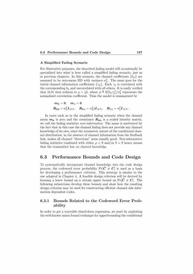
6.3 Performance Bounds and Code Design 197
A Simplified Fading Scenario
For illustrative purposes, the described fading model will occasionally bespecialized into what is here called a simplified fading scenario, just asin previous chapters. In this scenario, the channel coefficients hk areassumed to be zero-mean IID with variance σ2
h. The same goes for theinitial channel information coefficients γk. Each γk is correlated withthe corresponding hk and uncorrelated with all others. It is easily verifiedthat (6.9) then reduces to ρ = |ρ|, where ρ , E[hkγ∗
k ]/σ2h represents the
normalized correlation coefficient. Thus the model is summarized by
mh = 0, mγ = 0
Rhh = σ2hIMN , Rhγ = σ2
hρIMN , Rγγ = σ2hIMN .
In cases such as in the simplified fading scenario when the channelmean mh is zero and the covariance Rhh is a scaled identity matrix,we call the fading statistics non-informative. The name is motivated bythe fact that in this case the channel fading does not provide any channelknowledge of its own, since the symmetric nature of the conditional chan-nel distribution, in the absence of channel information from the feedbacklink, makes all channel “directions” seem equally good. Non-informativefading statistics combined with either ρ = 0 and/or b = 0 hence meansthat the transmitter has no channel knowledge.
6.3 Performance Bounds and Code Design
To systematically incorporate channel knowledge into the code designprocess, the codeword error probability Pr[C 6= C] is used as a basisfor developing a performance criterion. This strategy is similar to theone adopted in Chapter 4. A feasible design criterion will be derived byforming a lower bound on a certain upper bound on Pr[C 6= C]. Thefollowing subsections develop these bounds and show how the resultingdesign criterion may be used for constructing efficient channel side infor-mation dependent codes.
6.3.1 Bounds Related to the Codeword Error Prob-ability
In order to get a tractable closed-form expression, we start by exploitingthe well-known union bound technique for upperbounding the conditional

198 6 Quantized Channel Feedback: Design Approach II
codeword error probability Pr[C 6= C|i,h] so as to obtain
Pr[C 6= C|i,h] ≤ 1
K
∑
k 6=l
P (C(i)k → C
(i)l |i,h)
=1
K
∑
k 6=l
Q
(
‖H∗(C(i)k − C
(i)l )‖F
2√
σ2/2
)
≤ 1
2K
∑
k 6=l
e−‖H∗(C(i)k
−C(i)l
)‖2F/(4σ2)
=1
K
∑
k<l
e−‖H∗(C(i)k
−C(i)l
)‖2F/(4σ2) , (6.10)
where P (C(i)k → C
(i)l |i,h), with k 6= l, denotes the pairwise error proba-
bility
Pr[‖X − H∗C
(i)k ‖2
F > ‖X − H∗C(i)l ‖2
F |C = C(i)k , i,h
](6.11)
and where the Gaussian tail function Q(x) is upperbounded [WJ90, p. 84]by 0.5 exp(−x2/2). Note that (6.11) represents the probability that the
ML decoding metric for C(i)l is smaller than the metric for C
(i)k , con-
ditioned on h, i and on the event that the transmitted codeword is
C = C(i)k .
An upper bound PUB(C(i)) on the codeword error probability isobtained by averaging over i and h in (6.10) to arrive at
Pr[C 6= C] ≤ 1
K
∑
k<l
Ei,h
[e−‖H∗(C
(i)k
−C(i)l
)‖2F/(4σ2)
]
=1
K
∑
k<l
Ei,γ
[
Eh
[e−‖H∗(C
(i)k
−C(i)l
)‖2F/(4σ2)|i,γ
]]
=1
K
∑
k<l
Ei,γ
[
Eh
[e−‖H∗(C
(i)k
−C(i)l
)‖2F/(4σ2)|γ
]]
(6.12)
, PUB(C(i)) ,
where the second equality is due to the fact that h, γ and i form a Markov
chain h – γ – i. Comparing Eh
[e−‖H∗(C
(i)k
−C(i)l
)‖2F/(4σ2)|γ
]with the
definition of the previous codeword pair criterion in (4.7), while keepingin mind that γ corresponds to ζ in (4.7), shows that (4.11) can be used
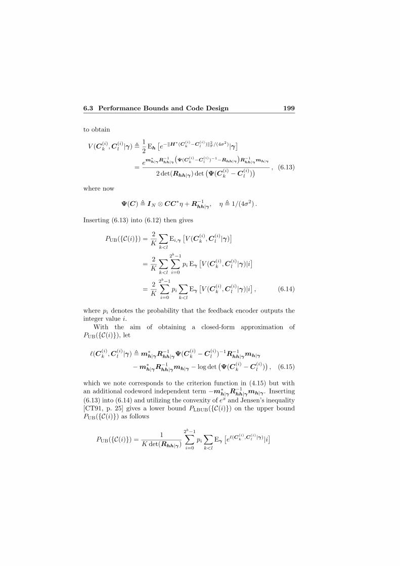
6.3 Performance Bounds and Code Design 199
to obtain
V (C(i)k ,C
(i)l |γ) ,
1
2Eh
[e−‖H∗(C
(i)k
−C(i)l
)‖2F/(4σ2)|γ
]
=em∗
h|γR−1hh|γ
(Ψ(C
(i)k
−C(i)l
)−1−Rhh|γ
)R−1
hh|γmh|γ
2 det(Rhh|γ) det(Ψ(C
(i)k − C
(i)l )) , (6.13)
where now
Ψ(C) , IN ⊗ CC∗η + R−1hh|γ , η , 1/(4σ2) .
Inserting (6.13) into (6.12) then gives
PUB(C(i)) =2
K
∑
k<l
Ei,γ
[V (C
(i)k ,C
(i)l |γ)
]
=2
K
∑
k<l
2b−1∑
i=0
pi Eγ
[V (C
(i)k ,C
(i)l |γ)|i
]
=2
K
2b−1∑
i=0
pi
∑
k<l
Eγ
[V (C
(i)k ,C
(i)l |γ)|i
], (6.14)
where pi denotes the probability that the feedback encoder outputs theinteger value i.
With the aim of obtaining a closed-form approximation ofPUB(C(i)), let
`(C(i)k ,C
(i)l |γ) , m∗
h|γR−1hh|γΨ(C
(i)k − C
(i)l )−1R−1
hh|γmh|γ
− m∗h|γR−1
hh|γmh|γ − log det(Ψ(C
(i)k − C
(i)l )), (6.15)
which we note corresponds to the criterion function in (4.15) but withan additional codeword independent term −m∗
h|γR−1hh|γmh|γ . Inserting
(6.13) into (6.14) and utilizing the convexity of ex and Jensen’s inequality[CT91, p. 25] gives a lower bound PLBUB(C(i)) on the upper boundPUB(C(i)) as follows
PUB(C(i)) =1
K det(Rhh|γ)
2b−1∑
i=0
pi
∑
k<l
Eγ
[e`(C
(i)k
,C(i)l
|γ)|i]

200 6 Quantized Channel Feedback: Design Approach II
≥ 1
K det(Rhh|γ)
2b−1∑
i=0
pi
∑
k<l
eEγ [`(C(i)k
,C(i)l
|γ)|i] (6.16)
, PLBUB(C(i)) ,
which holds with equality if `(C(i)k ,C
(i)l |γ), for a fixed i, is a constant.
In general, the lower bound PLBUB(C(i)) approximates PUB(C(i))well when the variance of `(C
(i)k ,C
(i)l |γ) conditioned on i is small. From
(6.15) it is seen that this is the case if the quantization is dense (sothat mh|γ is concentrated around Eγ [mh|γ |i]), σ2 is low and/or thecorrelation between γ and h is small. The final form of PLBUB(C(i))is obtained by utilizing the relation tr(AB) = tr(BA) and the fact thatRhh|γ is constant with respect to γ, as evident from (6.7). With a slightabuse of notation, the exponent in (6.16) can then be rewritten as
Eγ
[`(C
(i)k ,C
(i)l |γ)|i
]= Eγ
[m∗
h|γR−1hh|γΨ−1R−1
hh|γmh|γ |i]
− Eγ [m∗h|γR−1
hh|γmh|γ |i] − Eγ
[log det(Ψ)|i
]
= tr(Ψ−1R−1hh|γ Eγ [mh|γm∗
h|γ |i]R−1hh|γ)
− tr(R−1hh|γ Eγ [mh|γm∗
h|γ |i]) − log det(Ψ) . (6.17)
Using (6.6) it is easily verified that Eγ [mh|γm∗h|γ |i] can be written in
terms of the first and second order moments E[γ|i], E[γγ∗|i]. In the codedesign process, both these moments are replaced by the correspondingsample estimates taken from a Monte-Carlo simulation of the encoder inthe feedback link.
Note that the development in this subsection is general in the sensethat it does not rely on the assumption of a specific space-time code.Hence, the derived bounds can be used for assessing the performance ofany space-time code.
6.3.2 The Code Design Problem
In principle, as suggested in our work in [JSO02b], it is possible to con-struct codes by minimizing PUB(C(i)) with respect to the codewords,while satisfying the output power constraint. However, the computa-tional complexity of such an approach is challenging, to say the least,since the conditional expectation in (6.14) is not available in closed-formand since it depends on the codewords to be optimized. Motivated by

6.3 Performance Bounds and Code Design 201
the fact that PLBUB(C(i)) approximates PUB(C(i)) well in certaincases, we therefore take on an alternative approach in which the goal isto minimize PLBUB(C(i)). This criterion function is more suitable froma computational point of view since the conditional expectations do notdepend on the codewords and can hence be evaluated prior to the codesearch.
Unstructured codes, linear dispersive codes and weighted OSTBC, asdescribed in Section 3.2, are considered. Design procedures for these codetypes are developed below.
Unstructured Codes
Note from (6.16) and the power constraint (6.3) that the design problemdecouples and hence each unstructured code C(i) can be optimized sepa-rately from all others without loss of optimality. Consequently, based on(6.16) and (6.17), the design criterion is defined as
Wq(C|i) ,∑
k<l
Vq(Ck − Cl|i) , (6.18)
where C ,[C1 C2 · · · CK
]contains K arbitrary codewords and
Vq(C|i) ,etr(Ψ(C)−1R−1
hh|γEγ [mh|γm∗
h|γ |i]R−1hh|γ
)
det(Ψ(C)). (6.19)
The index “q” has here been introduced to emphasize that quantizedfeedback is considered. For the present case of unstructured codes, weminimize PLBUB(C(i)), subject to the power constraint in (6.3), bydesigning the codes as
C(i) = arg min
C
‖C‖2F=PK log2(K)
Wq(C|i), i = 0, · · · , 2b − 1 , (6.20)
where the codewords in C(i) correspond to the ith code C(i). A strategy
for numerically solving (6.20) will be presented in Section 6.5.Observe that the solution to (6.20) is not unique. Clearly, all code-
word matrices can be multiplied from the right by a common L × Lunitary matrix without affecting neither the cost function nor the powerconstraint. However, if desired, this ambiguity can be removed by im-posing a lower triangular structure onto one of the codewords.

202 6 Quantized Channel Feedback: Design Approach II
Note also that the above criterion function is closely related to theone that was derived in Chapter 4 based on the assumption that h|ζ iscomplex Gaussian. In fact, if Rhh|γ and Eγ [mh|γm∗
h|γ |i] in (6.19) are
replaced with Rhh|ζ and mh|ζm∗h|ζ , respectively, then Vq(Ck − Cl|i)
is equal to the corresponding term V (Ck − Cl|ζ) in (4.14). Hence, thecriterion functions in (6.20) and in the corresponding design problem forunstructured codes in (4.18) differ only in the choice of certain parame-ters, but not in structure.
Design procedures based on the present criterion function are alsoeasily developed for both linear dispersive codes as well as weighted OS-TBC. This since the design procedures may be directly inferred from(4.20) and (4.26), respectively, by simply modifying the constituent cri-terion functions. For completeness, the specifics for each code type aregiven below.
Linear Dispersive Codes
From the performance criterion in (6.18) and from the previously de-scribed design procedure given by (4.20) it is clear that the weights
B(i)m Ld
m=1 in the ith linear dispersive code may be designed as
B(i) = arg min
B
‖B‖2F=P log2(K)
Wq(C(B)|i) , (6.21)
where
B ,[B1 B2 · · · BLd
]
B(i)
,
[
B(i)1 B
(i)2 · · · B
(i)Ld
]
C(B) ,
[∑Ld
m=1 Bms(1)m
∑Ld
m=1 Bms(2)m · · · ∑Ld
m=1 Bms(K)m
]
,
with s(k)m , m = 1, 2, · · · , Ld representing the symbol sequence corre-
sponding to the kth codeword.
Weighted OSTBC
Similarly to as in Section 4.5, the transmit weighting can be designedby only considering the worst codeword pairs in the fixed OSTB code

6.3 Performance Bounds and Code Design 203
CkKk=1. In other words, after substituting Ck = WCk into (6.18),
only the terms corresponding to codeword pairs such that
A(Ck, Cl) , (Ck − Cl)(Ck − Cl)∗ = µminIM ′ , k 6= l
are retained. Here, µmin denotes the minimum value over all µkl ,∑Lo
m=1
(s(k)m − s
(l)m
)2. Let
`q(WW ∗, µkl|i) , log(Vq(W (Ck − Cl)|i)
).
Since the remaining terms are all equal, they are minimized by designing
the codebook of transmit weighting matrices W (i)2b−1i=0 as
W (i) = arg minW
‖W ‖2F=Po
`q(WW ∗, µmin|i), i = 0, 1, · · · , 2b .
Just as in Section 4.5, the above optimization problem may be solved intwo steps. The first step is to re-parameterize using WW ∗ = Z andthen solve the equivalent problem
Z(i) = arg minZ
Z=Z∗0
rank(Z)≤minM ′,Mtr(Z)=Po
`q(Z|i), i = 0, 1, · · · , 2b , (6.22)
where
`q(Z|i) , `q(Z, µmin|i)
= tr((
(IN ⊗ Z)η + R−1hh|γ
)−1R−1
hh|γ Eγ [mh|γm∗h|γ |i]R−1
hh|γ
)
− log det((IN ⊗ Z)η + R−1
hh|γ
), (6.23)
with η , µmin/(4σ2). In the second and final step, the transmit weighting
is obtained as W (i) =(Z(i)
)1/2, where (·)1/2 denotes a matrix square-
root.Because of the previously mentioned similarity between Vq(Ck−Cl|i)
in (6.19) and V (Ck − Cl|ζ) in (4.14), it is not difficult to show thatbasically all the theoretical results based on the latter criterion functioncarry over, sometimes in somewhat modified form, to the present case.In particular, it should be noted that also (6.22) is a convex optimizationproblem if the transmit weighting is square, i.e., M ′ = M . Moreover,it is straightforward to modify the algorithm for a simplified scenariodescribed in Section 4.7 to deal with the new criterion function. Thus,the transmit weight design problem given by (6.22) can be efficientlysolved using simple modifications of techniques discussed earlier.

204 6 Quantized Channel Feedback: Design Approach II
6.4 Unstructured Codes – Analysis and In-
terpretations
It is in general a difficult task to explicitly characterize the optimal setof codewords. However, in a few special cases it is possible to derivesome properties that the optimal codewords must posses. The analysispresented in this section focuses entirely on unstructured codes. It is how-ever straightforward to perform similar analyses for the two other codetypes. The results to be derived herein are important for understandingthe behavior of the transmitter and also help to explain the simulationresults in Section 6.7.
Several of the following cases under consideration are asymptotic inthe sense that optimal unstructured codes obtained from (6.20) are tobe investigated as some parameter tends to a limit. In such asymptoticcases, we rely, similarly to as in Appendix 4.A, on a theorem [SS89,p. 221] stating that it is possible to interchange the order of the limitand minimization operator in an optimization problem provided that 1)the criterion function converges uniformly over the feasibility set to alimit function, 2) the feasibility set is compact, 3) the limit function iscontinuous and has a unique global minimum within the feasibility set. Ifthe limit function possesses several (i.e., non-unique) global minima thenthe theorem reduces to a weaker form claiming that an asymptoticallyoptimal solution belongs to the set of global minima of the limit function.
Applying the weaker form of the theorem to the design proceduremeans that (6.20) may be studied with Wq(C|i) replaced by the corre-sponding limit function. Using techniques similar to the ones used inAppendix 4.A, it can be shown that such an interchange of order is al-lowed. Therefore, to simplify the presentation we will in the followingomit the proofs on uniform convergence and instead tacitly assume thatthe limit function can be used for deriving the asymptotic properties ofthe optimal code.
6.4.1 Perfect Channel Knowledge
Consider first the case of perfect initial channel information, i.e., Rhγ →Rhγ , where Rhγ is such that ρ → 1. Introduce the M × N channel
estimate matrix MH|γ , E[H|γ], also obtained by rearranging mh|γ
so as to satisfy the relation mh|γ = vec(MH|γ). A Taylor expansionof log(Vq(Ck − Cl|i)) then shows that a criterion function equivalent to

6.4 Unstructured Codes – Analysis and Interpretations 205
Wq(C|i) in (6.20) may be written as
W1(C|i) , Wq(C|i)/etr(R−1hh|γ
E[mh|γm∗h|γ |i])+log det(Rhh|γ)
=∑
k<l
e−η tr(IN⊗Akl(E[mh|γm∗h|γ |i]+Rhh|γ))+O(η2‖Rhh|γ‖)
=∑
k<l
e−η tr(Akl(E[MH|γM∗H|γ |i]+Rhh|γ))+O(η2‖Rhh|γ‖) , (6.24)
where O(·) is the big ordo operator and where
Akl , (Ck − Cl)(Ck − Cl)∗
Rhh|γ , E[(H − MH|γ)(H − MH|γ)∗|γ] .
Note that Rhh|γ can also be expressed as the sum of the N blocks of sizeM ×M on the diagonal of Rhh|γ , explaining why O(η2‖Rhh|γ‖) may be
replaced by O(η2‖Rhh|γ‖). Observing that Akl is bounded due to thepower constraint, dropping η from the ordo and making use of the Taylorexpansion ex = 1 + O(x) leads to
W1(C|i) =∑
k<l
e−η tr(Akl E[MH|γM∗H|γ |i])eO(‖Rhh|γ‖)
=∑
k<l
e−η tr(Akl E[MH|γM∗H|γ |i]) + O(‖Rhh|γ‖) .
As previously noted, Rhγ → Rhγ implies ‖Rhh|γ‖ → 0 and hence also
‖Rhh|γ‖ → 0. Thus, W1(C|i) converges to the limit function
W1(C|i) , limRhγ→Rhγ
W1(C|i)
=∑
k<l
e−η tr((Ck−Cl)(Ck−Cl)∗Ri) , (6.25)
whereRi , E[MH|γM
∗H|γ |i] ,
with MH|γ , limRhγ→RhγMH|γ .
Before discussing the above result, we consider the related case ofperfect channel knowledge at the transmitter. Hence, in addition toperfect initial channel information, assume the feedback is such that

206 6 Quantized Channel Feedback: Design Approach II
the quantization is infinitely dense in the γ domain1. In such a case,E[MH|γM∗
H|γ |i] can be expected to be essentially equal to MH|γM∗H|γ
for a γ corresponding to some infinitely small encoder region Si. Weformalize this as follows. Assume a sequence of quantization schemes
is chosen so that the corresponding sequence of encoder regions S (b)i ,
b = 0, 1, · · · , for a particular i, all enclose a certain fixed point γ in thevector space C
MN×1. Let
rb , maxγ∈S
(b)i
‖γ − γ‖
be the radius of a sphere centered at γ that encloses S (b)i and assume that
S(b)i becomes smaller as b is increased in the sense that limb→∞ rb = 0.
From the mean-value theorem it can then be shown that
E[MH|γM∗H|γ |i] =
∫
S(b)i
MH|γM∗H|γpγ|i(γ|i)dγ
= MH|γM∗H|γ + O(rb) , (6.26)
where MH|γ , E[H|γ = γ]. With (6.24) as a starting point, inserting(6.26) into (6.24), using the Taylor expansion ex = 1 + O(x) and takingthe limit (Rhγ , rb) → (Rhγ , 0) gives a limit function exactly like the onein (6.25) but now with
Ri , MH|γM∗H|γ ,
where MH|γ , limRhγ→RhγMH|γ .
Based on the limit functions, properties of the optimal code are de-rived as follows. Let UΛU ∗ be the EVD of Ri, where U is a uni-tary M × M matrix with columns containing the eigenvectors of Ri
and Λ is an M × M diagonal matrix with ordered diagonal elementsλ1 ≥ λ2 ≥ · · · ≥ λr > λr+1 = · · · = λM = 0 representing the eigenvalues.Here, r is the rank of Ri. Due to the unitary nature of U , the optimiza-tion problem with (6.25) as criterion function can be re-parameterizedbased on Ck , U∗Ck and C , U∗
C, without affecting the power con-
1Obviously, the phase-only quantization scheme used as an example in this workdoes not belong to this category.

6.4 Unstructured Codes – Analysis and Interpretations 207
straint since ‖C‖2F = ‖C‖2
F, to arrive at
W1(U C|i) =∑
k<l
e−η tr((Ck−Cl)(Ck−Cl)∗Λ)
=∑
k<l
e−η∑r
m=1 λm‖c(k)m −c(l)
m ‖2
, (6.27)
where (c(k)m )∗ is the mth row of Ck. It is seen that the value of the
asymptotic criterion function in (6.27) does not depend on c(k)m K
k=1,m = r + 1, · · · ,M , i.e., the M − r last rows of the re-parameterizedcodewords. Also, observe that letting these rows be non-zero decreasesthe available output power that can be allocated to the remaining rowsand is hence wasteful. Since the optimal cost decreases as a function of
the output power it can be concluded that the rows c(k)m M
m=r+1 in allcodewords must be zero. On the other hand, for the r first (potentiallynon-zero) rows, each eigenvalue λm weighs the corresponding row in C.Because of the weighting, rows with a large eigenvalue are favored whichin turn means that the energy allocated to a particular row tends to belarger for a row with a large eigenvalue than for one with a small eigen-value. After solving the re-parameterized problem in (6.27), the code is
formed as C(i) = U C
(i), where C
(i)denotes the optimal C. Consequently,
for the asymptotically optimal code, the transmitted power is distributedonly along the first r eigenvectors of Ri, with typically large power in“eigen-directions” with large eigenvalues.
The above result is worth elaborating upon. Assume perfect channelknowledge at the transmitter so that Ri = MH|γM
∗H|γ . From the SVD
theorem [HJ96, p. 414], recall that U and √
λmrm=1 also represent the
left singular eigenvectors and singular values, respectively, of MH|γ . Dueto the assumption of perfect channel knowledge, MH|γ is now essentiallyequal to the channel matrix H and we may base the following discussionon the commonly used SVD of the channel matrix. Hence, since the last
M − r rows of C(i)
are zero, the transmission is confined to the spacespanned by the left singular eigenvectors corresponding to the non-zerosingular values of the channel matrix. Moreover, the power tends to beprimarily allocated to strong eigen-directions, i.e., where the correspond-ing singular values are large. Such a behavior makes sense since thereis no point wasting energy in directions which contribute little or notat all to the received signal. In particular, for the case of one receiveantenna we have r = 1 and the optimal codewords are therefore of rank

208 6 Quantized Channel Feedback: Design Approach II
one, resulting in a beamforming type of transmission.In comparison, an information theoretic result derived in e.g. [Tel95]
states that capacity in a MIMO system can be achieved by transmittingalong the left singular eigenvectors of the channel matrix with a power al-location obeying a water-filling distribution. The water-filling procedureensures that the power allocated along strong eigen-directions is largeand that no power is wasted on eigen-directions having singular valuesequal to zero. This clearly agrees well with the perfect channel knowledgeproperty derived above.
Note also that although the perfect channel knowledge case in thepresent work and in Section 4.6 may seem to be similar, it is risky to drawconclusions for the problem at hand based on the earlier developmentin that section, where the totally different weighted OSTBC structurewas considered. In particular, if the channel knowledge is perfect, theasymptotically optimal codewords mentioned in Section 4.6 are always ofrank one, regardless of the number of receive antennas, while the same isin general not true for the code structure herein, unless only one receiveantenna is used.
6.4.2 Low SNR
The low SNR case is defined as P/σ2 = 4Pη → 0. For technical reasons,we start with re-parameterizing the optimization problem in (6.20) basedon Ck , Ck/
√P and C , C/
√P . With η replaced by Pη, (6.24) can
be used as a starting point for deriving the first order (in terms of Pη)Taylor expansion
W2(C|i) , Wq(√
P C|i)=∑
k<l
e−Pη tr(Akl(E[MH|γM∗H|γ |i]+Rhh|γ))+O(P 2η2)
=∑
k<l
1 − Pη tr(Akl(E[MH|γM∗H|γ |i] + Rhh|γ)) + O(P 2η2)
= −Pη tr((∑
k<l
Akl
)
(E[MH|γM∗H|γ |i] + Rhh|γ)
)
+K(K − 1)
2+ O(P 2η2) , (6.28)
where Akl , (Ck − Cl)(Ck − Cl)∗ and K(K − 1)/2 is the number of
different codeword pairs. From (6.28) it is clear that the asymptotic prop-

6.4 Unstructured Codes – Analysis and Interpretations 209
erties of the optimal code can be analyzed by considering maximizationof the limit function
W2(C|i) , limPη→0
−1
Pη
(
W2(C|i) −K(K − 1)
2
)
= tr((∑
k<l
Akl
)
(E[MH|γM∗H|γ |i] + Rhh|γ)
)
.
Assume that the rank of E[MH|γM∗H|γ |i] + Rhh|γ is r and let UΛU∗
represent the corresponding EVD. With a similar approach as was usedto obtain (6.27), the limit function can be re-parameterized using Ck ,
U∗Ck, C , U∗C and written as
W2(U C|i) =
r∑
m=1
λm
∑
k<l
‖c(k)m − c(l)
m ‖2 . (6.29)
Note that also in this case must the M − r last rows c(k)m K
k=1, m =r + 1, · · · ,M be equal to zero for optimality. To proceed, define
f(P ) , maxc(k)
m Kk=1
∑Kk=1 ‖c(k)
m ‖2=P
∑
k<l
‖c(k)m − c(l)
m ‖2
and again re-parameterize based on c(k) = c(k)m /
√
P to obtain
f(P ) = P maxc(k)K
k=1∑K
k=1 ‖c(k)‖2=1
∑
k<l
‖c(k) − c(l)‖2
= αP , (6.30)
where α is a constant which can be interpreted as a measure of howwell the constellation of rows are separated. Optimization of the rows in(6.29) can be carried out by first optimizing each row separately under a
fixed power constraint∑K
k=1 ‖c(k)m ‖2 = Pm, producing the concentrated
criterion function f(Pm), and then using f(Pm) for optimizing the powervalues Pm subject to
∑rk=1 Pm = K log2(K). By utilizing (6.30), it is
seen that the optimal power values may hence be obtained as
Pmrm=1 = arg max
Pmrm=1∑r
m=1 Pm=K log2(K)
r∑
m=1
λmf(Pm)

210 6 Quantized Channel Feedback: Design Approach II
= arg maxPmr
m=1∑rm=1 Pm=K log2(K)
r∑
m=1
λmPm . (6.31)
For simplicity, assume that λ1 is strictly larger than all other eigenvalues.It is then easily verified that in the optimal solution of (6.31), all power isallocated to the first eigen-direction, i.e., P1 = K log2(K), Pm = 0,m =2, · · · ,M . Thus, only the first row of an optimal C is non-zero and,because of C = U C, the asymptotically optimal code distributes all poweralong the strongest eigenvector of E[MH|γM∗
H|γ |i] + Rhh|γ .
A comparison with the perfect channel knowledge case reveals severalsimilarities. Studying (6.27) and (6.29) we see that the perfect channelknowledge and low SNR cases are closely related. In both cases the trans-mission power is distributed along some eigen-directions and the amountof energy in each eigen-direction depends on weights in the form of certaineigenvalues. However, they primarily differ in that in the low SNR caseonly the strongest eigen-direction is used while for the perfect channelknowledge case the energy may be distributed among all eigen-directionswith non-zero eigenvalues. In addition, for the low SNR case, the EVD isbased not only on a feedback dependent term E[MH|γM∗
H|γ |i] but also
on an additional term Rhh|γ .
6.4.3 No Feedback / No Channel Knowledge
In this section, the cases of no feedback and no channel knowledge areanalyzed. Consider first a scenario with no feedback, or more precisely,assume that b = 0 and/or Rhγ = 0. In other words, the channel in-formation at the transmitter is statistically independent of γ and hencealso of h. Consequently, E[mh|γm∗
h|γ |i] = E[mh|γm∗h|γ ] = mhm∗
h andRhh|γ = Rhh, which means that the design criterion no longer dependson the initial channel information γ. In order to also remove the ex-ponential in (6.19), the scenario is further specialized by assuming thatmh = 0. These assumptions model a non-line-of-sight scenario with afeedback delay that is very long compared to the coherence time of thechannel. After scaling with 1/det(Rhh) the design criterion in (6.18)then takes on the equivalent form
W3(C|i) ,∑
k<l
1
det(IMN + Rhh(IN ⊗ Akl)η), (6.32)

6.4 Unstructured Codes – Analysis and Interpretations 211
which can be shown to be a valid upper bound on the codeword errorprobability also when Rhh is singular. Now, assume fading such thatthe columns hl of H are uncorrelated but with the same transmittercovariance RT , E[hlh
∗l ] or, equivalently, that the channel covariance
matrix has the Kronecker structure Rhh = IN ⊗ RT. This so-called“one-ring” channel model may be appropriate in scenarios where thetransmitter is placed above the rooftops far away from scatterers while atthe receiver there is plenty of local scattering [SFGK00]. The Kroneckerstructure of Rhh means that (6.32) simplifies to
W3(C|i) =∑
k<l
1
detN (IM + ηRTAkl). (6.33)
To see how the criterion function in (6.33) affects the code design, letUΛU∗ represent the EVD of RT, with Λ = diag(λ1, · · · , λM ), UU∗ =IM . Furthermore, use the relation det(I + AB) = det(I + BA), foundin Appendix C, to express the determinant as
det(IM + ηRTAkl) = det(IL + η
M∑
m=1
λm(c(k)m − c(l)
m )(c(k)m − c(l)
m )∗),
where (c(k)m )∗ is the mth row of Ck , U∗Ck. Hence, we again see that
the transmission is along some eigen-directions, given by the columnsof U , and that the corresponding eigenvalues serve to weigh the eigen-directions.
Unfortunately, further development is complicated by the large num-ber of terms in (6.33). Therefore, in order to obtain tractable expressions,a special case with only two codewords, C1 and C2, is studied next. Itis reasonable to assume that this provides valuable insight also into thegeneral case of an arbitrary number of codewords. In the derivation, anecessary condition on the codewords of an optimal code will be utilized.The following lemma summarizes the result, which is valid for any num-ber of codewords and for the general assumptions described in the systemmodel.
Lemma 1 (A Necessary Condition for Optimality) Let CkKk=1
denote the codewords in an optimal code that solves the design prob-lem in (6.20). These codewords then satisfy the necessary condition
K∑
k=1
Ck = 0M×L , (6.34)

212 6 Quantized Channel Feedback: Design Approach II
regardless of the quality of the channel information.
Proof:The proof relies on the KKT conditions [BS93, p. 162] that are nec-
essary for optimality. In order to obtain compact expressions, it is con-venient to first define some additional notation for derivatives. Let ∂f
∂X
denote a matrix where element (k, l), is equal to ∂f∂[X]kl
, i.e., it is equal
to the derivative of f , f(X) with respect to element [X]kl of X. Sincethe elements in the matrices of interest are typically complex-valued, thenotion of a complex derivative [Kay93, p. 517] is utilized and defined as
∂f
∂x,
1
2
(∂f
∂ re(x)− j
∂f
∂ im(x)
)
, (6.35)
where j is the imaginary unit, f is a function of x, x is complex-valuedand re(x) and im(x) denote the real and imaginary part of x, respectively.
Let∂Wq
∂Ck(C) denote the derivative of Wq(C|i) with respect to the
complex-valued elements of Ck, evaluated at C. With δn representingthe Kronecker delta function, the derivative can be written as
∂Wq
∂Ck(C) =
∑
k′<l′
k′=k or l′=k
(1 − 2δl′−k)V ′q(Ck′ − Cl′) , (6.36)
where, as shown in Appendix 6.A, the derivative V ′q(C) of Vq(C|i), eval-
uated at C, is equal to
V ′q(C) ,
∂Vq
∂C(C) = −ηVq(C|i)(ΩC)c . (6.37)
Here, (·)c denotes the complex conjugate and Ω represents the sum ofthe N blocks of size M × M on the diagonal of
Ψ(C)−1 + Ψ(C)−1R−1hh|γ E[mh|γm∗
h|γ |i]R−1hh|γΨ(C)−1 .
It is now straightforward to verify that the KKT conditions applied toWq(C|i) and the power constraint ‖C‖2
F = PK log2(K) lead to the fol-lowing system of equations
∂Wq
∂Ck(C) + µ(Ck)c = 0M×L, k = 1, 2, · · · ,K (6.38)
K∑
k=1
‖Ck‖2F = PK log2(K) , (6.39)

6.4 Unstructured Codes – Analysis and Interpretations 213
where µ is a Lagrange multiplier. Adding all K equations in (6.38) and
noting that∑
k∂Wq
∂Ck(C) = 0M×L, due to the coefficients (1 − 2δl′−k) in
(6.36), gives
µ
K∑
k=1
Ck = 0M×L . (6.40)
It is realized that µ must be non-zero, otherwise (6.38) and (6.39) imply
that all K gradients∂Wq
∂Ck(C) are identically zero for a code that satisfies
the power constraint. The latter is only possible if all codewords are allequal since it can easily be checked that for any other code Wq(αC|i) is astrictly decreasing function of α, meaning that the gradient is non-zero.Clearly, the codewords cannot all be equal in an optimal code. Hence, µis non-zero and (6.40) reduces to the necessary condition in (6.34), whichall optimal codes must obey.
Returning to the K = 2 codeword case, the lemma is utilized for sim-plifying W3(C|i) in (6.33). We solve for C2 in (6.34) and hence substituteC2 = −C1 into W3(C|i) to arrive at the equivalent problem
A12 = arg maxA12
rank(A12)≤r
tr A12=4P
det(IM + RTA12/(4σ2)) , (6.41)
where r = minM,L denotes the maximum possible rank of A12 =(C1 − C2)(C1 − C2)
∗ = 4C1C∗1. Ignoring for a moment the rank con-
straint, this is a classical optimization problem that also occurs, for ex-ample, when computing the capacity of a set of parallel channels withcolored Gaussian noise. It turns out that the rank constraint is eas-ily handled within the scope of previous classical derivations (comparewith how a thin transmit weighting matrix is handled in Section 4.7).Hence, with 4σ2(RT)−1 here playing the role of the covariance of the col-ored noise, it follows from [CT91, p. 253-255] that the optimal solutionis A12 = V DV ∗, where V is an M × r matrix containing the r firstcolumns of U and D is a diagonal r × r matrix with elements given bythe water-filling solution
dm = maxν − 4σ2λ−1m , 0, m = 1, 2, · · · , r . (6.42)
Here, ν is a Lagrange multiplier that can be determined from the powerconstraint. Thus, since A12 = 4C1C
∗1, the optimal codewords can be
taken asC1 = −C2 = 0.5
[
V D1/2 0M×(L−r)
]

214 6 Quantized Channel Feedback: Design Approach II
and we conclude that the transmission power is distributed along the rfirst eigen-vectors of RT.
A related water-filling result concerning the properties of linear disper-sive codes in correlated fading scenarios is found in [SP01]. That result,as well as the solution of (6.41), can also be used to directly determine asemi closed-form expression for the optimal transmit weighting matrix inthe weighted OSTBC design procedure given by (4.26). This since (4.26)reduces to an optimization problem of the same form as (6.41), whenmh|ζ is zero and Rhh|ζ has the same structure as the covariance matrixRhh considered herein.
Specializing the one-ring model by assuming non-informative fadingstatistics Rhh = IN⊗σ2
hIM = σ2hIMN leads to the no channel knowledge
case. Since the eigenvalues λm = σ2h of RT then are all equal, it follows
from (6.42) that D is also a scaled identity matrix and hence the poweris distributed equally in all eigen-directions. Thus, for M ≤ L (M ≥ L)the rows (columns) of C1 and C2 must be orthogonal and of equal mag-nitude. Another way of formulating this is to say that the singular valuesof each codeword are equal. In particular, note that M = L means thatthe codewords are unitary matrices. How the statement generalizes forcodes with more than two codewords is still an open issue. However,the experimental code construction results later presented in Section 6.6indicate that the derived orthogonality property hold in many cases. Theappealing properties of unitary codewords have also been noted in pre-vious work such as [BV01], where it is shown that unitary codewordsminimize the union bound of the codeword error probability under theassumption of an unknown channel at both the transmitter and receiver.This is in line with previous information theoretic based arguments in[MH99] for a similar non-coherent scenario.
6.4.4 High SNR
The high SNR case is defined as P/σ2 = 4Pη → ∞. It is assumed in thefollowing derivation that the codeword matrices are wide, i.e., M ≤ L. Inpractice, this is not a particularly restrictive assumption since space-timecodewords with shorter duration are unable to satisfy the rank criterion[GFBK99, TSC98] and hence cannot reach the maximum diversity orderof the system.
Similar to as was done in the low SNR derivation, the optimizationproblem in (6.20) is re-parameterized using Ck , Ck/
√P and C ,
C/√
P . Furthermore, the resulting power constraint ‖C‖2F = K log2(K)

6.4 Unstructured Codes – Analysis and Interpretations 215
is augmented with an additional constraint
Akl , (Ck − Cl)(Ck − Cl)∗ εIM
to ensure that Akl is invertible. Here, ε is a positive constant. It canbe argued that, for sufficiently small ε, introducing the additional con-straint does not change the asymptotically optimal solution. Hence, theproperties of the asymptotically optimal code that will be derived nextare valid also for the original optimization problem, see Appendix 4.A.1concerning a similar approach. Based on the Taylor expansions
tr((IN ⊗ AklPη + R−1
hh|γ)−1Rhh|γ E[mh|γm∗h|γ |i]−1Rhh|γ
)
= O(P−1η−1ε−1)
log det(IN ⊗ AklPη + R−1hh|γ) = MN log(Pη)
+N log det(Akl) + O(P−1η−1ε−1) ,
an equivalent criterion function can be expressed as
W4(C|i) , Wq(√
P C|i)eMN log(Pη)
=∑
k<l
e−N log det(Akl)+O(P−1η−1ε−1)
=∑
k<l
e−N log det(Akl) + O(P−1η−1ε−1) .
Thus, letting P/σ2 = 4Pη → ∞, while keeping ε constant and sufficientlysmall, we conclude that the code properties can be inferred from the limitfunction
W4(C|i) , limPη→∞
W4(C|i)
=∑
k<l
1
detN ((Ck − Cl)(Ck − Cl)∗). (6.43)
It is seen that the differences Ck −Cl must all be full-rank in the asymp-totically optimal code. Otherwise, the determinant of (Ck − Cl)(Ck −Cl)
∗ is zero for at least one codeword pair and the corresponding term in(6.43) would be infinitely large, implying that this cannot be the optimalsolution. Consequently, performing the code design at a sufficiently highSNR ensures full-diversity space-time codes.

216 6 Quantized Channel Feedback: Design Approach II
Note also that the criterion in (6.43) does not depend on neither thefeedback information i nor the channel statistics. Thus, as the SNRincreases the optimal code makes less and less use of channel knowledgeand in the limit does not use it at all. A similar observation was madein connect with information theoretic results depicted in Figure 2.5. Thesimilarities with the previous no channel knowledge case suggest that theoptimal code tends to a no channel knowledge like code with codewordswhose rows are often more or less orthogonal. This can be proved for thecase of two codeword codes (K = 2) by arguing similarly as was done tosolve (6.41).
6.4.5 Parameter Insensitivity of Some Codes
In general, the codes designed in this work depend on a number of pa-rameters in addition to the explicit channel information contained in i.The power budget P , noise variance σ2, covariance and cross-covariancematrices and the number of receive antennas N are all examples of suchparameters. This dependence may be a drawback in situations were theparameters are not known, or are not known with great accuracy, sincethe performance typically degrades when the assumptions in the designprocess are different from those in the scenario in which the codes areused. It would therefore be beneficial to have codes that remain optimaleven if the mentioned parameters are varied. Although the codes are ingeneral not parameter independent, it is in this section made plausiblethat under certain circumstances the proposed code design process willgenerate codes that work well regardless of the values of the parameters.These theoretical findings are in line with code design and simulationresults presented in later sections.
Below, we will show that, for the simplified fading scenario with no
channel knowledge, a code C , √
P/P Ck satisfies the KKT condi-
tions (6.38) - (6.39), regardless of the values of σ2, σ2h, P and N , if the
codewords Ck are such that they satisfy the KKT conditions for someparameters σ2 = σ2, σ2
h = σ2h, P = P , N = N and in addition obey the
orthogonality property
Akl , (Ck − Cl)(Ck − Cl)∗ = λklIM , k 6= l , (6.44)
with λkl = λ constant over all codeword pairs. As shown in Section 6.6,the orthogonality property in (6.44) is a characteristic of one of the con-
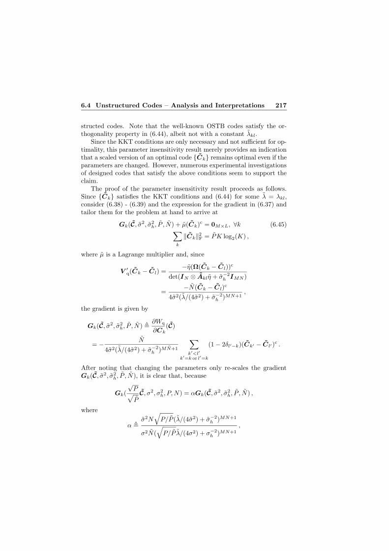
6.4 Unstructured Codes – Analysis and Interpretations 217
structed codes. Note that the well-known OSTB codes satisfy the or-thogonality property in (6.44), albeit not with a constant λkl.
Since the KKT conditions are only necessary and not sufficient for op-timality, this parameter insensitivity result merely provides an indicationthat a scaled version of an optimal code Ck remains optimal even if theparameters are changed. However, numerous experimental investigationsof designed codes that satisfy the above conditions seem to support theclaim.
The proof of the parameter insensitivity result proceeds as follows.Since Ck satisfies the KKT conditions and (6.44) for some λ = λkl,consider (6.38) - (6.39) and the expression for the gradient in (6.37) andtailor them for the problem at hand to arrive at
Gk(C, σ2, σ2h, P , N) + µ(Ck)c = 0M×L, ∀k (6.45)
∑
k
‖Ck‖2F = PK log2(K) ,
where µ is a Lagrange multiplier and, since
V ′q(Ck − Cl) =
−η(Ω(Ck − Cl))c
det(IN ⊗ Aklη + σ−2h IMN )
=−N(Ck − Cl)
c
4σ2(λ/(4σ2) + σ−2h )MN+1
,
the gradient is given by
Gk(C, σ2, σ2h, P , N) ,
∂Wq
∂Ck(C)
= − N
4σ2(λ/(4σ2) + σ−2h )MN+1
∑
k′<l′
k′=k or l′=k
(1 − 2δl′−k)(Ck′ − Cl′)c .
After noting that changing the parameters only re-scales the gradientGk(C, σ2, σ2
h, P , N), it is clear that, because
Gk(
√P
√
PC, σ2, σ2
h, P,N) = αGk(C, σ2, σ2h, P , N) ,
where
α ,σ2N
√
P/P (λ/(4σ2) + σ−2h )MN+1
σ2N(√
P/P λ/(4σ2) + σ−2h )MN+1
,

218 6 Quantized Channel Feedback: Design Approach II
the code √
P/P Ck and the Lagrange multiplier µ = αµ simply scale
the left hand side of (6.45) and hence the KKT conditions are satisfied.This concludes the proof.
6.4.6 A Symmetric Feedback Scenario
It often makes sense to design the feedback link so that the quantiza-tion is, in some sense, symmetric. For example, in the commonly as-sumed Rayleigh fading scenario, the phase of each channel coefficient isuniformly distributed and hence it is reasonable to use an encoder thatquantizes the phase uniformly over the phase interval [0, 2π). This mo-tivates the partial phase combining [HP98] type of method of this work.The feedback method in the closed-loop mode of the WCDMA system[3GP02b] is another example of uniform phase quantization. The en-coder regions of these quantization schemes exhibit symmetries in thesense that they are rotated copies of each other. This section investigateshow similar rotational symmetries affect the code design and how theycan be exploited for reducing the computational complexity of the de-sign method. A similar concept of symmetric feedback was introduced inSection 2.6.3 for simplifying numerical evaluation of a channel capacityexpression.
Recall that a unitary matrix may correspond to a rotation. With thisin mind, we say that the feedback scenario is symmetric if E[mh|γm∗
h|γ |i]and Rhh|γ can be written on the form
E[mh|γm∗h|γ |i] = D ⊗ QiRQ∗
i (6.46)
Rhh|γ = D ⊗ IM , (6.47)
where Qi is a unitary M ×M matrix that depends on i, R is a constantM × M matrix, D , diag(d1, d2, · · · , dN ) and D , diag(d1, d2, · · · , dN )for some arbitrary dnN
n=1 and dnNn=1, respectively.
The above conditions affect the code design as follows. By using theKronecker relations (C.3) and (C.4) in Appendix C, repeated below forconvenience
(X1 ⊗ X2)(X3 ⊗ X4) = X1X3 ⊗ X2X4
(X1 ⊗ X2)−1 = X−1
1 ⊗ X−12 ,
and assuming (6.46), (6.47) hold, it is possible to write
R−1hh|γ E[mh|γm∗
h|γ |i]R−1hh|γ = DD−2 ⊗ QiRQ∗
i ,

6.4 Unstructured Codes – Analysis and Interpretations 219
which inserted into (6.18) leads to the re-parameterized criterion function
Wq(QiC|i) =∑
k<l
etr((IN⊗Aklη+D−1⊗IM )−1(DD−2⊗R))
det(IN ⊗ Aklη + D−1 ⊗ IM )(6.48)
and power constraint ‖C‖2F = PK log2(K), where C , Q∗
i C, Ck ,
Q∗i Ck, Akl , (Ck − Cl)(Ck − Cl)
∗.Clearly, (6.48) is independent of i and the original code design problem
may therefore be solved by first minimizing (6.48) with respect to Ck,subject to the power constraint, and then extracting the ith code throughthe linear mapping C
(i) = QiC, where C now represents the optimalsolution in the re-parameterized problem. Hence, the inherent symmetryof the feedback carries over to a corresponding symmetry of the codes.Because all codes are easily derived by means of a linear transformationfrom the single code in C, this result can be utilized to substantiallyexpedite the design process and reduce the memory required to store thecode.
Symmetric Feedback in the Simplified Fading Scenario
As an illustrative example of a symmetric feedback situation, consider thefeedback scheme in this work operating in the simplified fading scenariowith N = 1 receive antenna. Since the relative phases are uniformlyquantized, the codebook vectors in (6.5) that the encoder uses can beexpressed in terms of the first codebook vector as ˆγ(i) = Qi
ˆγ(0), i =0, · · · , 2b − 1, where
Qi , diag(1, ejφi0(i) , ejφi1(i) , · · · , ejφiMN−2(i))
rotates ˆγ(0) to the desired position. To see that also the encoder regionsare rotations of each other, let γ belong to encoder region S0 and notethat
ε(Qkγ) = arg mini
‖Qkγ/γ1 − Qiˆγ(0)‖2
= arg mini
‖γ/γ1 − Q∗kQi
ˆγ(0)‖2 = k ,
since Q∗kQi ∈ Qi and Q∗
kQk = IM = Q0. This means that foreach point γ in S0 there is a corresponding rotated point Qkγ in Sk
(the converse can also be established in a similar manner, comparewith Appendix 2.D.3) and we conclude that Si are rotated versions
220 6 Quantized Channel Feedback: Design Approach II
of S0. Together with the zero-mean IID complex Gaussian distribu-tion’s invariance to a unitary linear mapping, i.e., the PDF of γ hasthe property pγ(γ) = pγ(Qiγ), it follows from similar derivations as inAppendix 2.D.1 that the conditional PDF of γ|i satisfies the followingrelation pγ|i(γ|0) = pγ|i(Qiγ|i). Using this relation it is readily shownthat
E[mh|γm∗h|γ |i] = |ρ|2 E[γγ∗|i] = ρ2Qi E[γγ∗|0]Q∗
i
= QiRQ∗i ,
with R = ρ2 E[γγ∗|0] and, consequently, the first symmetric feedbackcondition in (6.46) is satisfied. The second symmetric feedback condition(6.47) is also satisfied since for the simplified fading scenario it followsfrom (6.7) that Rhh|γ = σ2
h(1 − |ρ|2)IMN = σ2h(1 − ρ2)IN ⊗ IM . Thus,
we have shown that the partial phase combining type of feedback schemeused in the simplified fading scenario indeed constitutes a symmetricfeedback situation and hence all the 2b different codes can be derivedfrom a single code Ck by means of known linear transformations. Thiswill be utilized later, both in Section 6.6 to describe constructed codesin a compact manner as well as for simulation purposes in Section 6.7.
6.5 Numerical Optimization
The design procedures for unstructured and linear dispersive codes de-scribed in Section 6.3.2 represent non-convex optimization problems,which are in general difficult to solve. The present section describeshow numerical gradient search [BS93] type of techniques can be utilizedfor “solving” these optimization problems. With such an approach, thesolution can only be expected to be locally optimal. To remedy this,the chance of finding the global optimum is improved by repeating thegradient search several times, each time initiated differently, and pickingthe best of the resulting solutions. Although the technique is tailored tothe application under consideration, it is similar in structure to the opti-mization procedure utilized in [FGW74] for the design of efficient signalconstellations.
6.5.1 Unstructured Codes
The numerical optimization procedure for unstructured codes implementsa gradient search which updates the code C by taking a step along the

6.5 Numerical Optimization 221
direction of the negative gradient of Wq(C|i). The result is thereafternormalized so as to satisfy the output power constraint of the codewordconstellation. Starting with an initial guess C0 of the solution, the code-word constellation is hence updated, for n = 0, 1, · · · , according to
Cn+1 =
√
PK log2(K)(
Cn − µn
(∂Wq
∂C(Cn)
)c)
‖Cn − µn
(∂Wq
∂C(Cn)
)c
‖F
, (6.49)
where µn is the so-called step size and, based on (6.36), the derivativeswith respect to all the codewords have been collected in a matrix repre-senting the gradient as
∂Wq
∂C(C) =
[∂Wq
∂C1(C)
∂Wq
∂C2(C) · · · ∂Wq
∂CK(C)]
.
The complex conjugate in (6.49) is due to the negative sign of the imag-inary part in the definition of the complex derivative in (6.35).
An appropriate step size is obtained by using successively smaller val-ues of µn until the design criterion is found to have decreased. Several al-ternative methods for choosing the step size exist in the literature [BS93].A candidate solution is found by iterating (6.49) until convergence.
The gradient search is repeated several times using different C0 set atrandom. Finally, the best of the resulting candidate solutions is chosenand designated as the constructed code C
(i). The random initializationstrategy can be complemented in various ways. For example, a C0 corre-sponding to an OSTB code or beamforming could also be used. In thisway, the constructed code is guaranteed to perform equal or better (asmeasured by the criterion function) than either of these two well-knowntransmission methods.
6.5.2 Linear Dispersive Codes
It should be clear that a similar numerical optimization technique can beused to “solve” the design problem for linear dispersive codes in (6.21).The major difference compared with the previous gradient search in (6.49)is that the gradient is now instead evaluated with respect to the transmitweights in B.
To explicitly describe the gradient search in the present case, let∂Wq
∂Bm(B) denote the derivative of Wq(C(B)|i) with respect to the mth

222 6 Quantized Channel Feedback: Design Approach II
weighting matrix Bm, evaluated at B. Since Ck =∑Ld
m=1 Bms(k)m , the
derivative is easily inferred from (6.37). Hence, it is realized that
∂Wq
∂Bm(B) =
∑
k<l
(s(k)m − s(l)
m )V ′q
(Ld∑
m′=1
Bm′(s(k)m′ − s
(l)m′)
)
.
Collect now all the Ld derivatives and form the gradient as
∂Wq
∂B(B) =
[∂Wq
∂B1(B)
∂Wq
∂B2(B) · · · ∂Wq
∂BLd(B)]
.
Similarly to as in the case of unstructured codes, the gradient searchstarts with an initial guess B0 of the solution and updates the weightingmatrices according to
Bn+1 =
√
P log2(K)(
Bn − µn
(∂Wq
∂B(Bn)
)c)
‖Bn − µn
(∂Wq
∂B(Bn)
)c
‖F
, (6.50)
until convergence.
6.5.3 Computational Complexity Issues
It is clear that the numerical optimization may be performed off-line.Thus, although the computing power needed for the codeword search issubstantial, the resulting transmission scheme can be efficiently imple-mented via the use of lookup tables.
Consider first the case of unstructured codes. The time it takes tocomplete the code design increases with the size of the problem. Formodest values of M , L and K, a solution is obtained within a reasonableshort time period. The main bottleneck is typically the computation ofthe design criterion and gradient when the number of codewords K islarge. Since the number of terms in the design criterion and gradientgrows quadratically with K (c.f. (6.28)), the time it takes to performthe update in (6.49) quickly becomes prohibitive, resulting in an essen-tially unsolvable code design problem. Nevertheless, we have managedto construct M = 8, L = 8 unstructured codes with up to K = 4096codewords using the techniques presented in this chapter. Of course, thedesign of codes with codewords of smaller dimension and at least thismany codewords is also feasible.

6.5 Numerical Optimization 223
Both high and low rate codes are possible, depending on the lengthL of the codewords. For an M = 2, L = 2 code and assuming a max-imum of 4096 codewords, the rate may be as high as log2(4096)/2 = 6bits per channel use while for the M = 8, L = 8 case a more moder-ate rate of log2(4096)/8 = 1.5 bits per channel use is possible. To ob-tain much higher rates it may be necessary to use other design methodsthat do not rely on pairwise error probabilities and possibly also reducethe number of parameters in the problem by introducing additional con-straints/structure. The use of linear dispersive codes is one example ofhow structure may be introduced to drastically reduce the number of pa-rameters that need to be optimized. However, the benefits of structuretypically come at the price of lower performance since structure generallylimits the degrees of freedom in the design.
The problems associated with the rapid growth of the computationalcomplexity with respect to K may also be circumvented by employinglinear dispersive codes. A viable strategy is then to design the weight-ing matrices so as to maximize the information theoretic capacity of asuitable channel. Similarly as was done in [HH02b] for the no channelknowledge case, the well-known MIMO capacity formula [Tel95], or therelated expression in (2.7), can be used with channel information incor-porated into the design through the statistics of the channel and feedback(c.f. mean and covariance feedback [VM01]).
It should be noted that such criteria are only appropriate for longblock lengths with the transmitted codeword experiencing many differentchannel realizations, the latter because the relevant capacity formulasrely on the assumption of ergodic fading. In other words, code designmethods based on these criteria are geared toward applications whichcan tolerate a rather high processing delay. Our design procedures, onthe other hand, are intended for significantly shorter block lengths, thustargeting delay sensitive applications, and do not assume coding overdifferent channel realizations. Furthermore, a fundamental assumptionbehind capacity maximizing code construction methods as in [HH02b] isthat the designed code is concatenated with an outer code to obtain lowerror probability. In contrast, the code design methods proposed hereinstrive for minimizing the error probability directly.
Another important issue is decoding complexity. As evident from(6.2), the unstructured codes designed in this work require an exhaustivesearch over all codewords. The resulting computational complexity maybe tolerable for codes with a moderate number of codewords, but forhigh rate applications the high decoding complexity essentially excludes
224 6 Quantized Channel Feedback: Design Approach II
the use of unstructured codes. Linear dispersive codes may then be amore appealing choice since they permit, as pointed out in Section 3.2.2the use of decoding algorithms [VH02, JMO03] with significantly lowercomplexity than an exhaustive search.
Obviously, weighted OSTBC is an even better choice if low computa-tional complexity is the only issue under consideration. This applies bothto the transmit weight design procedure as well as to the ML detectionalgorithm.
6.6 Code Design Results
The design method described by (6.20) and implemented as (6.49) hasbeen used for constructing numerous channel side information dependentunstructured codes. This section presents a few illustrative examples ofsuch constructed codes and their properties. In addition, properties of acouple of linear dispersive codes, designed using (6.21), are also presented.All codes presented in this section were designed under the assumptionof the simplified fading scenario with N = 1 receive antenna, a powerbudget P = 1 and fading variance σ2
h = 1.
A Channel Side Information Dependent Unstructured Code
In Table 6.1, three unstructured M = 2, L = 2, K = 4 codes are pre-sented. The codes have been designed for a noise variance σ2 = 0.1, cor-responding to an SNR of 10 dB in the graph depicted in Figure 6.2, andusing an initial channel information quality ρ set to 0, 0.95 and 0.9999,respectively. In the two latter cases, b = 2 bits were used to quantizethe initial channel information using the phase quantization scheme de-scribed in Section 6.2.1. Only the codewords of the first code, C(0), areexplicitly displayed. This constitutes all needed codes in the no chan-nel knowledge ρ = 0 case. For the ρ = 0.95 and ρ = 0.9999 cases, thefeedback is symmetric, as explained in Section 6.4.6, and the remainingcodes C(i), i = 1, 2, 3 are hence obtained through the linear transforma-
tions C(i)k = QiC
(0)k , where Qi , diag(1, ejπi/2). All the codes in the
table together with their linearly transformed counterparts can be saidto form one channel side information dependent code.
The condition number κ(C(i)k ) (with respect to the spectral norm) of
each codeword C(i)k has been computed and the results are summarized
and displayed above the corresponding code. Since the condition number

6.6 Code Design Results 225
ρ = 0 ⇒ κ(C(0)k ) ≈ 1
C(0)1
−0.71126 + j0.36087 +0.40735 − j0.44435−0.58663 + j0.14285 −0.65934 + j0.44859
C(0)2
+0.01832 + j0.21581 +0.08399 + j0.97295+0.81098 + j0.54269 −0.18061 − j0.12080
C(0)3
+0.15579 + j0.09515 −0.94038 − j0.28723+0.20541 − j0.96129 −0.00773 − j0.18309
C(0)4
+0.53715 − j0.67183 +0.44904 − j0.24136−0.42976 + j0.27575 +0.84767 − j0.14470
ρ = 0.95 ⇒ κ(C(i)k ) ≈ 6
C(0)1
−0.92111 + j0.37685 −0.04889 − j0.10390−0.88850 + j0.32513 −0.30045 + j0.10687
C(0)2
+0.48440 + j0.49155 −0.03616 + j0.72504+0.67026 + j0.56673 −0.09747 + j0.46532
C(0)3
+0.24692 − j0.47884 −0.77306 − j0.34031+0.25685 − j0.72680 −0.55128 − j0.31430
C(0)4
+0.18980 − j0.38956 +0.85812 − j0.28083−0.03860 − j0.16506 +0.94920 − j0.25788
ρ = 0.9999 ⇒ κ(C(i)k ) > 104
C(0)1
−0.41928 + j0.80405 +0.24074 − j0.35123−0.41680 + j0.80166 +0.23961 − j0.35014
C(0)2
+0.40759 − j0.35120 −0.50008 − j0.68115+0.40569 − j0.35052 −0.49916 − j0.67815
C(0)3
−0.33466 − j0.68957 +0.61490 + j0.19504−0.33429 − j0.68668 +0.61289 + j0.19353
C(0)4
+0.34635 + j0.23672 −0.35556 + j0.83734+0.34539 + j0.23554 −0.35334 + j0.83476
Table 6.1: Constructed C(0) codes for different ρ. Design parameters:M = 2, L = 2, N = 1, K = 4, b = 2, P = 1, σ2 = 0.1.
is the ratio between the maximum and minimum singular value [HJ96,p. 442], it serves as a measure of how close the codewords are to unitaryand rank one matrices (the latter because there are only two singularvalues), respectively.
The condition number is seen to increase with ρ. In particular, since
κ(C(0)k ) ≈ 1 the codewords in the ρ = 0 code are all essentially scaled
unitary matrices, in line with the K = 2 no channel knowledge result de-rived in Section 6.4.3. Correspondingly, the almost perfect initial channelknowledge ρ = 0.9999 code has codewords with very high condition num-bers, meaning that the codewords are close to rank one. This is explainedby studying the eigenvalues of Ri = E[MH|γMH|γ |i] in (6.25). It canbe verified that the difference between the two eigenvalues is large andhence almost all power is allocated along the strongest eigen-direction,in good agreement with the discussion related to perfect initial channelinformation in Section 6.4.1.

226 6 Quantized Channel Feedback: Design Approach II
Properties in the No Channel Knowledge Case
No channel knowledge constitutes an important special case that war-rants further investigation. Table 6.2 presents some interesting proper-ties of a few constructed codes and, as benchmarks, corresponding rateone OSTB codes as found in [TJC99]. This time, both unstructured andlinear dispersive codes were designed. Because of the no channel knowl-
edge assumption, only the determinant term of `(C(i)k ,C
(i)l |γ) in (6.15)
remains, implying that PLBUB(C(i)) = PUB(C(i)) in (6.16). Hence,both design procedures now strive for minimizing an upper bound on theunion bound of the codeword error probability.
A BPSK signal constellation was used for the constituent informationsymbols in each OSTB and linear dispersive code. Every row representsa code with the first column displaying dimensions and the type of code,“U”, “L” and “O” stand for unstructured, linear dispersive and OSTBcode, respectively. In the second column, the spread of energy over thecodewords is measured using the ratio
εmaxC /εmin
C , maxk
‖Ck‖2F/min
k‖Ck‖2
F .
To measure how close the codewords are to unitary matrices, the thirdcolumn shows the maximum codeword condition number
κC , maxk
κ(Ck)
of each code. Similarly, in the fourth and fifth column,
εmaxA /εmin
A , maxk 6=l
‖Akl‖2F/min
k 6=l‖Akl‖2
F, κA , maxk 6=l
κ(Akl) ,
where we recall that Akl = (Ck − Cl)(Ck − Cl)∗. Together these two
measures show whether the code is parameter insensitive as defined bythe orthogonality property in (6.44). Finally, to facilitate a comparison ofthe performance at high SNR values, the last column displays the codinggain
CG ,
(∑
k<l
1
detN ((Ck − Cl)(Ck − Cl)∗)
)−1/(MN)
for each code. The definition of the coding gain stems from the fact thatat high SNR values the upper bound on the codeword error probabilityin (6.32) can, for the no channel knowledge case and assuming full di-versity codes that satisfy the rank criterion [TSC98], be approximated
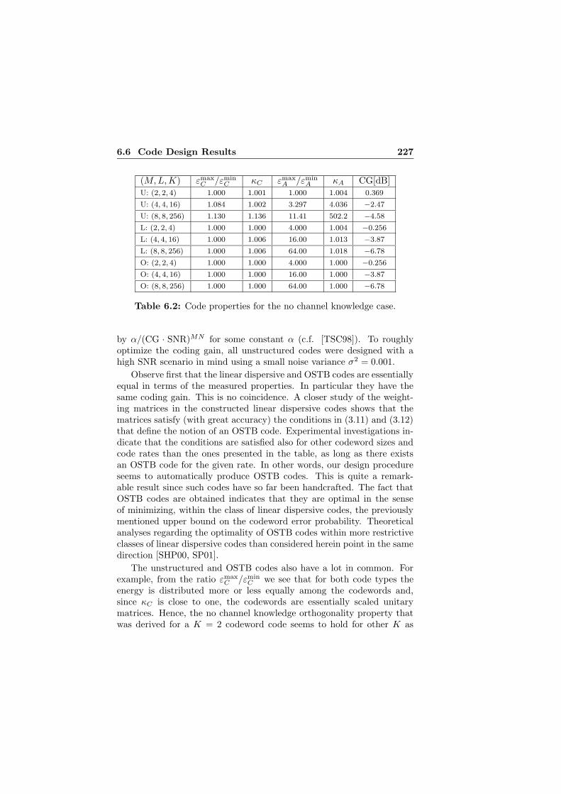
6.6 Code Design Results 227
(M,L,K) εmaxC /εmin
C κC εmaxA /εmin
A κA CG[dB]U: (2, 2, 4) 1.000 1.001 1.000 1.004 0.369
U: (4, 4, 16) 1.084 1.002 3.297 4.036 −2.47
U: (8, 8, 256) 1.130 1.136 11.41 502.2 −4.58
L: (2, 2, 4) 1.000 1.000 4.000 1.004 −0.256
L: (4, 4, 16) 1.000 1.006 16.00 1.013 −3.87
L: (8, 8, 256) 1.000 1.006 64.00 1.018 −6.78
O: (2, 2, 4) 1.000 1.000 4.000 1.000 −0.256
O: (4, 4, 16) 1.000 1.000 16.00 1.000 −3.87
O: (8, 8, 256) 1.000 1.000 64.00 1.000 −6.78
Table 6.2: Code properties for the no channel knowledge case.
by α/(CG · SNR)MN for some constant α (c.f. [TSC98]). To roughlyoptimize the coding gain, all unstructured codes were designed with ahigh SNR scenario in mind using a small noise variance σ2 = 0.001.
Observe first that the linear dispersive and OSTB codes are essentiallyequal in terms of the measured properties. In particular they have thesame coding gain. This is no coincidence. A closer study of the weight-ing matrices in the constructed linear dispersive codes shows that thematrices satisfy (with great accuracy) the conditions in (3.11) and (3.12)that define the notion of an OSTB code. Experimental investigations in-dicate that the conditions are satisfied also for other codeword sizes andcode rates than the ones presented in the table, as long as there existsan OSTB code for the given rate. In other words, our design procedureseems to automatically produce OSTB codes. This is quite a remark-able result since such codes have so far been handcrafted. The fact thatOSTB codes are obtained indicates that they are optimal in the senseof minimizing, within the class of linear dispersive codes, the previouslymentioned upper bound on the codeword error probability. Theoreticalanalyses regarding the optimality of OSTB codes within more restrictiveclasses of linear dispersive codes than considered herein point in the samedirection [SHP00, SP01].
The unstructured and OSTB codes also have a lot in common. Forexample, from the ratio εmax
C /εminC we see that for both code types the
energy is distributed more or less equally among the codewords and,since κC is close to one, the codewords are essentially scaled unitarymatrices. Hence, the no channel knowledge orthogonality property thatwas derived for a K = 2 codeword code seems to hold for other K as

228 6 Quantized Channel Feedback: Design Approach II
well. For the unstructured (2, 2, 4) code, κA ≈ 1, which means thatthere are constructed codes that even share the pairwise orthogonalityproperty (6.44) with the OSTB codes. Moreover, since εmax
A /εminA ≈ 1,
the scaling factor λkl is almost constant. The code therefore satisfies allthe requirements for the parameter insensitivity result to apply, whichprovides an indication that the code will perform well even if σ2, σ2
h, Pand N are changed. Tests conducted for various parameter values showthat this is indeed the case since the unstructured (2, 2, 4) code givesapproximately the same values of the criterion function as the solutionsobtained by performing the numerical optimization procedure. From theparameter insensitivity it follows that the codewords can be consideredto be the same as for the ρ = 0 code in Table 6.1.
Performance wise, however, the unstructured and OSTB codes differsignificantly, even in the present case of no channel knowledge. Theformer are seen to have consistently higher coding gains than the latter.For example, the unstructured (2, 2, 4) code is 0.6 dB better than thecorresponding OSTB code while the difference is 1.4 dB for the (4, 4, 16)codes. These numbers are also approximately confirmed by simulationresults in Section 6.7. Of course, the performance advantage exhibited bythe designed unstructured codes is to be expected considering the designfreedom offered by the absence of structural constraints.
6.7 Numerical Examples
To illustrate the performance of some constructed codes, simulations ofthe communication system in Section 6.2 were conducted for the sim-plified fading scenario using an M = 2 and M = 4 transmit antennasystem, respectively. To focus on a common situation in practice, N = 1receive antenna was assumed throughout the simulations. By consider-ing three different cases, ρ = 0 (no channel knowledge), ρ = 0.95 andρ = 0.9999 with b = 2 or b = 6 feedback bits, depending on the numberof transmit antennas, the impact of the channel information quality onthe performance was studied. Note that the ρ = 0 case also correspondsto an open-loop system for which conventional space-time codes are ap-propriate. Therefore, an OSTBC system was used as a benchmark. Acomparison with beamforming was also performed. Using beamforming,the transmitted signal can be written on the form c(n) = vs(n), wheres(n) represents the nth information bearing data symbol and v is a trans-mit weighting vector. For ideal beamforming the true channel h is used

6.7 Numerical Examples 229
as a weighting vector while for conventional beamforming v = ˆγ(i), withthe feedback encoder2 now defined as i = ε(γ) , arg maxk ‖γ∗ ˆγ(k)‖2
F.This choice of encoder serves to maximize the received signal power inthe case of perfect initial channel knowledge [HP98].
The remaining assumptions in the simulations were as follows. Forall the examined cases, equally probable bits were mapped into code-words/blocks of length L samples and conveyed over the spatially uncor-related flat Rayleigh fading channel. An energy of P = 1 per informationbit was used. The variance of the channel coefficients was set at σ2
h = 1.In the case of the systems employing OSTBC or beamforming, a BPSKsignal constellation was employed. To make fair comparisons, the effec-tive data rates of the constructed codes were fixed at 1 information bitper channel use. The SNR was measured for the conventional OSTBCsystem and defined as
SNR ,E[‖H∗C‖2
F]
LNσ2,
where C =√
Po/MC with C denoting the codeword output from theOSTB encoder. The expression for the SNR is equal to the total receivedaverage signal energy, divided by the total average noise energy.
We start with investigating the performance of unstructured codes.Unstructured codes will then be compared with linear dispersive codesand weighted OSTBC by means of one representative simulation example.
Unstructured Codes versus Conventional Schemes
In Figure 6.2, the codeword/block error probability (BLER) as a func-tion of the SNR is depicted for some unstructured codes, OSTBC andbeamforming. An M = 2, L = 2 system is considered. The channel infor-mation was coarsely quantized using b = b = 2 bits per complex-valueddimension. The ρ = 0 code was taken from Table 6.1 while all otherunstructured codes were designed based on the same parameter values asused in the simulations.
Clearly, the performance of the constructed codes, regardless of chan-nel information quality ρ, is significantly better than the performance ofconventional OSTBC and beamforming. In particular, it should be notedthat the OSTB code is outperformed by the unstructured codes even ifthere is no channel knowledge. As predicted by Table 6.2, a gain on the
2For an M = 2, N = 1 system, this encoder is equivalent to the one in (6.4).

230 6 Quantized Channel Feedback: Design Approach II
−5 0 5 10 15 20 2510−5
10−4
10−3
10−2
10−1
100
Conv. OSTBCUnstructured Code: ρ=0Unstructured Code: ρ=0.95Unstructured Code: ρ=0.9999Conv. beamforming: ρ=0.95Conv. beamforming: ρ=0.9999Ideal beamforming
PSfrag replacements
BLE
R
SNR [dB]
Figure 6.2: Performance comparisons for an M = 2, L = 2, N = 1, b = 2system.
order of 0.6 - 0.8 dB compared with OSTBC is observed for high SNRvalues using the ρ = 0 code. A similar gain for the constructed channelside information dependent ρ = 0.9999 code compared with the corre-sponding conventional beamforming method is also seen. With higherSNR, the curve for the ρ = 0.95 code (eventually also the ρ = 0.9999code) approaches the one for the no channel knowledge ρ = 0 code. Thisagrees well with the asymptotic high SNR result in Section 6.4.4 statingthat channel knowledge is used less and less as the SNR is increased. Infact, the two channel side information dependent codes tend to the ρ = 0code, since the latter can be viewed as parameter insensitive, and hencedesigned at an arbitrary SNR.
Figure 6.3 shows how the performance is affected if the number oftransmit antennas and the code length are increased to M = 4 and L = 4,respectively. By using b = b/3 = 2 bits, the quantization is roughly as

6.7 Numerical Examples 231
−5 0 5 10 15 2010−5
10−4
10−3
10−2
10−1
100
Conv. OSTBCUnstructured Code: ρ=0Unstructured Code: ρ=0.95Unstructured Code: ρ=0.9999Conv. beamforming: ρ=0.95Conv. beamforming: ρ=0.9999Ideal beamforming
PSfrag replacements
BLE
R
SNR [dB]
Figure 6.3: Performance comparisons for an M = 4, L = 4, N = 1, b = 6system.
coarse as in the previous figure. As expected, the gains due to channelknowledge increase substantially with more transmit antennas. Again,the 1.4 dB coding gain in Table 6.2 agrees well with simulated results.It is also interesting to note that even though the unstructured ρ =0.9999 code is based on coarsely quantized channel side information, it issignificantly better than ideal beamforming, which has access to perfect(i.e., non-quantized) channel state information. Thus, the proposed codedesign procedure succeeds in exploiting the unstructured nature of thecode for compensating for the imperfections of the channel feedback.

232 6 Quantized Channel Feedback: Design Approach II
Comparing the Three Code Structures
Design procedures for both linear dispersive codes as well as weightedOSTBC have also been implemented. Linear dispersive codes were de-signed using the gradient search based optimization algorithm in (6.50).For weighted OSTBC, the transmit weight design procedure in (6.22) wasimplemented by means of an interior point algorithm (c.f. (2.54)) thatfinds the global optimal solution.
−5 0 5 10 15 20
10−4
10−3
10−2
10−1
100
Conv. OSTBCWeighted OSTBC: ρ=0.9999Linear dispersive code: ρ=0.9999Unstructured code: ρ=0.9999Ideal beamforming
PSfrag replacements
BLE
R
SNR [dB]
Figure 6.4: Illustrating how the choice of code structure affects the perfor-mance for an M = 2, L = 2, N = 1, b = 2 system.
To give an idea of how the choice of code structure influences theperformance, constructed codes of the three code types are compared inFigure 6.4 for a system using M = 2 transmit antennas, N = 1 receiveantennas, L = 2 and b = 2 feedback bits, under similar conditions asfor the previous graphs. The quality of the initial channel information ishere arbitrarily set to ρ = 0.9999, i.e., it is essentially perfect.
As expected, the unstructured code is better than the two other code

6.8 Conclusions 233
types. What may be more surprising is that the linear dispersive codeand weighted OSTBC basically have the same performance. Numericalresults not presented here show that this is also the case also for othervalues of ρ. Indeed, for the extreme case of no channel knowledge, it isknown from Section 6.6 that the linear dispersive code is equivalent withOSTBC.
Preliminary experimental investigations indicate that linear dispersivecodes and weighted OSTBC exhibit similar performance in many differentscenarios. Thus, it may seem like linear dispersive codes offer little, ifany, performance advantage over weighted OSTBC. However, keep inmind that the former code type exists for all possible combinations ofantenna array sizes and data rates whereas weighted OSTBC is to alarge degree limited by the fact that an OSTB code with the maximumdata rate of two real-valued information symbols per channel use onlyexists for the case of two transmit antennas, as previously discussed inSection 3.2.3. A thin transmit weighting matrix, i.e., M ′ < M , mayto some extent offset this limitation. Nevertheless, it is reasonable toexpect that linear dispersive codes have clear performance advantagesover weighted OSTBC for systems with more than two transmit antennaswhen the required symbol rate is higher than the low rate of one generallyconsidered in the present section.
6.8 Conclusions
This work considered the design and analysis of space-time block codesutilizing non-perfect quantized channel side information. A new designcriterion was derived that directly takes the quantized nature of the chan-nel side information into account, thus avoiding heuristic modificationsas in the previous chapter. While the focus was on unstructured blockcodes, design procedures for linear dispersive codes and weighted OSTBCwere also proposed and implemented.
The constructed unstructured codes showed better performance thanboth conventional OSTBC as well as beamforming, even if there was nochannel knowledge at the transmitter. In the case of no channel knowl-edge, the design procedure for linear dispersive codes was seen to auto-matically produce OSTB codes, which is interesting since OSTB codespreviously have been handcrafted. Further investigations, experimentalas well as theoretical, are however needed to more fully understand themechanisms behind this result.

234 6 Quantized Channel Feedback: Design Approach II
Appendix 6.A The Gradient of Vq(C|i)The gradient of Vq(C|i) with respect to the parameters in C will
now be derived. In order to simplify the notation, let R ,
R−1hh|γ E[mh|γm∗
h|γ |i]R−1hh|γ , Ψ , Ψ(C) and drop the subscript of
Rhh|γ . For later reference, note the easily verifiable complex derivativerelations
∂x
∂x= 1,
∂xc
∂x= 0 , (6.51)
where x is a complex-valued scalar. Observe that the second relation of(6.51) means that any function of xc can be treated as a constant.
By evaluating the complex derivative with respect to element [C]kl ofC and making use of the identities [Kay93, p. 73]
∂X(θ)−1
∂θ= −X(θ)−1 ∂X(θ)
∂θX(θ)−1 (6.52)
∂ log det(X(θ))
∂θ= tr
(
X(θ)−1 ∂X(θ)
∂θ
)
, (6.53)
as well as (6.51) and the fact that tr(AB) = tr(BA) we have
∂ log(Vq(C|i)
)
∂[C]kl= −η tr
(Ψ−1(IN ⊗ e
(M)k (e
(L)l )∗C∗)
)
−η tr(
Ψ−1(IN ⊗ e
(M)k (e
(L)l )∗C∗
)Ψ−1R
)
= −η tr(Ψ−1(IN ⊗ e
(M)k (e
(L)l )∗C∗)
)
−η tr(Ψ−1RΨ−1(IN ⊗ e
(M)k (e
(L)l )∗C∗)
)
= −η
N∑
n=1
tr(Ωn(e
(M)k (e
(L)l )∗C∗)
)
= −η(e(L)l )∗C∗
(N∑
n=1
Ωn
)
e(M)k , (6.54)
where Ωn represents the nth block of size M × M on the diagonal ofΨ−1+Ψ−1RΨ−1. The first equality is due to the fact that differentiatingeach element of C with respect to [C]kl yields
∂C
∂[C]kl= e
(M)k (e
(L)l )∗ ,

6.A The Gradient of Vq(C|i) 235
where e(K)k denotes the kth column of IK . After collecting the derivatives
(6.54) in a matrix it is straightforward to show that
∂ log(Vq(C)
)
∂C= −η(ΩC)c ,
where Ω =∑N
n=1 Ωn. The gradient of Vq(C|i) is finally obtained as
∂Vq(C|i)∂C
= −ηVq(C|i)(ΩC)c .


Appendix A
Acronyms
BER Bit Error RateBLER BLock Error RateBPSK Binary Phase Shift KeyingCOVQ Channel Optimized Vector QuantizationDOA Direction Of ArrivalEVD EigenValue DecompositionFDD Frequency Division DuplexGSM Global System for Mobile communication or
Groupe Special MobileIID Independent and Identically DistributedKKT Karush-Kuhn-TuckerML Maximum LikelihoodMIMO Multi-Input-Multi-OutputMISO Multi-Input-Single-OutputMMSE Minimum Mean-Square ErrorOSTB Orthogonal Space-Time BlockOSTBC Orthogonal Space-Time Block CodingOFDM Orthogonal Frequency Division MultiplexingPAM Pulse Amplitude ModulationPDF Probability Density FunctionPMF Probability Mass Function

238 A Acronyms
QAM Quadrature Amplitude ModulationQPSK Quadrature Phase Shift KeyingSIMO Single-Input-Multi-OutputSISO Single-Input-Single-OutputSINR Signal-to-Interference-plus-Noise-RatioSNR Signal-to-Noise-RatioSVD Singular Value DecompositionTDD Time Division DuplexVQ Vector QuantizationWCDMA Wideband Code Division Multiple-Access

Appendix B
Notation
In this thesis, vectors and matrices are usually denoted by boldfacelowercase and uppercase letters, respectively. For example, x denotes avector while X represents a matrix. Vectors are generally representedby one-column matrices. A non-boldface calligraphic typeface is used todenote sets, e.g. A, B, C and so on. The list below and on the followingpages defines additional notation.
M × N The dimension of a matrix with M rows and Ncolumns.
XM×N An M × N matrix X.IM The identity matrix of dimension M × M .[X]kl The element on the kth row and lth column,
also referred to as element (k, l), of the matrixX.
XT The transpose of the matrix X.X∗ The complex conjugate transpose of the matrix
X.Xc The matrix obtained by taking the complex
conjugate on each element of the matrix X, i.e.,Xc = (X∗)T.
‖x‖ The Euclidean norm of a vector x, i.e., ‖x‖ =√x∗x.

240 B Notation
‖x‖K The norm of the vector x defined through‖x‖2
K = x∗Kx, where K is a positive definiteweight matrix.
‖X‖ The spectral norm of the matrix X, i.e., ‖X‖ =σmax, where σmax is the maximum singularvalue of X. Reduces to the usual Euclidiannorm if X is a vector.
‖X‖F The Frobenius norm of the matrix X, i.e.,
‖X‖F =√∑
k,l |[X]kl|2.rank(X) The rank of the matrix X.tr(X) The trace of the matrix X.det(X) The determinant of the matrix X.vec(X) The vectorized counterpart of the matrix X,
i.e., vec(X) is a vector containing the columnsof X stacked on top of each other. The columnsare ordered from the leftmost at the top to therightmost at the bottom.
diag(x1, x2, · · · , xM ) A diagonal matrix with elements x1, x2, · · · , xM
on the main diagonal.A B A − B is a positive semi definite matrix.A ⊗ B The Kronecker product of the matrices A and
B.δn The Kronecker delta function, i.e., δ0 = 1 and
zero otherwise. The argument n is here as-sumed to be an integer.
E[·] The expectation operator. Alternatively,Ex1,x2,···[·] may be used to emphasize that theexpectation is with respect to the random vari-ables x1, x2, · · · .
x|y Should be read as “x conditioned on y” exceptwhen it appears within a function name suchas for example f(x|y). In the latter case, x|y isused for emphasizing that f is a function of xparameterized by y.
E[x|y] Expected value of x conditioned on y, i.e., theexpectation is with respect to the PDF/PMFof x|y.

B Notation 241
Pr[E ] Probability of the event E . For example, Pr[i =k] represents the probability that the randomvariable i is equal to the deterministic value k.
x , a Denotes that x is equal to a per definition (andvice versa).
O(·) The big ordo operator.re(x) and im(x) Real and imaginary part of x, respectively.arg(x) The phase in radians, in the range −π to π, of
the complex-valued scalar x.arg minx f(x) The value of x that minimizes the criterion
function f(x).arg maxx f(x) The value of x that maximizes the criterion
function f(x).supx∈X f(x) The supremum of f(x) over the set of x such
that x ∈ X .exp(x) or ex The exponential function.log(x) The natural logarithm of x.log2(x) The base 2 logarithm of x.C The complex number field.R The real number field.Ak Denotes the set of all Ak.AkK
k=1 The set A1, A2, · · · , AK.|A| The cardinality of the set A, i.e., the number of
elements in the set.

Appendix C
Matrix Relations
Some useful formulas for manipulating expressions with matrices aregiven below. Proofs of all matrix relations are found in e.g. [SS89, Ap-pendix A] combined with [Gra81]. Let A, B and C denote matrices withdimensions so that the operations make sense. It then holds that
tr(AB) =(vec(A∗)
)∗vec(B) (C.1)
vec(ABC) = (CT ⊗ A) vec(B) (C.2)
(A ⊗ B)(C ⊗ D) = (AC ⊗ BD) (C.3)
(A ⊗ B)−1 = A−1 ⊗ B−1 (C.4)
det(I + AB) = det(I + BA) . (C.5)


Bibliography
[3GP02a] 3rd Generation Partnership Project ( 3GPP). Physicalchannels and mapping of transport channels onto physi-cal channels. Technical Report TS 25.211 V3.11.0, 2002.
[3GP02b] 3rd Generation Partnership Project ( 3GPP). Physicallayer procedures. Technical Report 3GPP TS 25.214V3.10.0, 2002.
[AHD+99] S. Anderson, B. Hagerman, H. Dam, U. Forssen, J. Karls-son, F. Kronestedt, S. Mazur, and K. J. Molnar. Adaptiveantennas for GSM and TDMA systems. IEEE PersonalCommunications, 6(3):74–86, June 1999.
[Ala98] S. M. Alamouti. A simple transmit diversity technique forwireless communications. IEEE Journal on Selected Areasin Communications, 16(8):1451–1458, October 1998.
[AMVW91] S. Andersson, M. Millnert, M. Viberg, and B. Wahlberg.An adaptive array for mobile communication systems.IEEE Transactions on Vehicular Technology, 40(1):230–236, February 1991.
[And63] T. W. Anderson. Asymptotic theory for principal compo-nent analysis. Annals of Mathematical Statistics, 34:122–148, February 1963.
[AO98] D. Astely and B. Ottersten. MLSE and spatio-temporalinterference rejection combining with antenna arrays. InProceedings European Signal Processing Conference, pages1341–1344, September 1998.

246 Bibliography
[ARU01] D. Agrawal, T. J. Richardson, and R. L. Urbanke.Multiple-antenna signal constellations for fading channels.IEEE Transactions on Information Theory, 47(6):2618–2626, September 2001.
[Asz95] D. Asztely. On antenna arrays in mobile communicationsystems, fast fading and GSM base station receiver al-gorithms. Master’s thesis, Royal Institute of Technology,February 1995.
[ATNS98] D. Agrawal, V. Tarokh, A. Naguib, and N. Seshadri.Space-time coded OFDM for high data-rate wireless com-munication over wideband channels. In Proc. IEEE Vehic-ular Technology Conference, pages 2232–2236, May 1998.
[BBH00] S. Baro, G. Bauch, and A. Hansmann. Improved codesfor space-time trellis-coded modulation. IEEE Communi-cations Letters, 4(1):20–22, January 2000.
[BCT01] E. Biglieri, G. Caire, and G. Taricco. Limiting perfor-mance of block-fading channels with multiple antennas.IEEE Transactions on Information Theory, 47(4):1273–1289, May 2001.
[BD91] W. R. Braun and U. Dersch. A physical mobile radio chan-nel model. IEEE Transactions on Vehicular Technology,40(2):472–482, May 1991.
[BFAOHY02] D. W. Bliss, K. W. Forsythe, III A. O. Hero, andA. F. Yegulalp. Environmental issues for MIMO capacity.IEEE Transactions on Signal Processing, 50(9):2128–2142,September 2002.
[Bin90] J. A. C. Bingham. Multicarrier modulation for data trans-mission: An idea whose time has come. IEEE Communi-cations Magazine, 28(5):5–14, May 1990.
[BJ95] G. E. Bottomley and K. Jamal. Adaptive arrays and MLSEequalization. In Proc. IEEE Vehicular Technology Confer-ence, pages 50–54, July 1995.
[Blu02] R. S. Blum. Some analytical tools for the design of space-time convolutional codes. IEEE Transactions on Commu-nications, 50(10):1593–1599, October 2002.

Bibliography 247
[BMC99] G. E. Bottomley, K. J. Molnar, and S. Chennakeshu. In-terference cancellation with an array processing MLSEreceiver. IEEE Transactions on Vehicular Technology,48(5):1321–1331, September 1999.
[BO02] M. Bengtsson and B. Ottersten. Handbook of Antennasin Wireless Communications, chapter 18. The ElectricalEngineering and Applied Signal Processing Series. CRCPress, 2002.
[BS91] P. Balaban and J. Salz. Dual diversity combining andequalization in digital cellular mobile radio. IEEE Trans-actions on Vehicular Technology, 40(2):342–354, May1991.
[BS93] M. S. Bazaraa and H. D. Sherali. Nonlinear Programming:Theory and Algorithms. John Wiley & Sons, 2nd edition,1993.
[Bur96] A. G. Burr. The multipath problem: An overview. In IEEColloquium on Multipath Countermeasures, pages 1/1–1/7,May 1996.
[BV99] S. Boyd and L. Vandenberghe. Introduction to convexoptimization with engineering applications. Course Notes,http://www.stanford.edu/class/ee364, 1999.
[BV01] M. Brehler and M. K. Varanasi. Asymptotic error prob-ability analysis of quadratic receivers in Rayleigh-fadingchannels with applications to a unified analysis of coherentand noncoherent space-time receivers. IEEE Transactionson Information Theory, 47(6):2383–2399, September 2001.
[CGS94] M. V. Clark, L. J. Greenstein, and W. K. Shafi. Opti-mum linear diversity receivers for mobile communications.IEEE Transactions on Vehicular Technology, 43(1):47–56,February 1994.
[Cim85] L. J. Cimini Jr. Analysis and simulation of a digital mobilechannel using orthogonal frequency division multiplexing.IEEE Transactions on Communications, COM-33(7):665–675, July 1985.

248 Bibliography
[CS99] G. Caire and S. Shamai. On the capacity of some chan-nels with channel state information. IEEE Transactions onInformation Theory, 45(6):2007–2019, September 1999.
[CT91] T. M. Cover and J. A. Thomas. Elements of InformationTheory. John Wiley & Sons, 1991.
[DGI+02] R. T. Derryberry, S. D. Gray, D. M. Ionescu, G. Mandyam,and B. Raghothaman. Transmit diversity in 3G CDMAsystems. IEEE Communications Magazine, 40(4):68–75,April 2002.
[DHSH00] A. Duel-Hallen, H. Shengquan, and H. Hallen. Long-rangeprediction of fading signals. IEEE Signal Processing Mag-azine, 17(3):62–75, May 2000.
[DN02] A. Das and P. Narayan. Capacities of time-varyingmultiple-access channels with side information. IEEETransactions on Information Theory, 48(1):4–25, January2002.
[ECS+98] R. B. Ertel, P. Cardieri, K. W. Sowerby, T. S. Rappa-port, and J. H. Reed. Overview of spatial channel modelsfor antenna array communication systems. IEEE PersonalCommunications, 5(1):10–22, February 1998.
[Far90] N. Farvardin. A study of vector quantization for noisychannels. IEEE Transactions on Information Theory,36(4):799–809, July 1990.
[FG98] G. J. Foschini and M. J. Gans. On limits of wireless com-munications in a fading environment when using multipleantennas. Wireless Personal Communications, 6(3):311–335, March 1998.
[FGW74] G. J. Foschini, R. D. Gitlin, and S. B. Weinstein. Op-timization of two-dimensional signal constellations in thepresence of Gaussian noise. IEEE Transactions on Com-munications, 22(1):28–37, January 1974.
[Fos96] G. J. Foschini. Layered space-time architecture for wirelesscommunication in a fading environment when using multi-element antennas. Bell Labs Technical Journal, pages 41–59, 1996.

Bibliography 249
[FU98] G. D. Forney Jr. and G. Ungerboeck. Modulation andcoding for linear Gaussian channels. IEEE Transactionson Information Theory, 44(6):2384–2415, October 1998.
[FV91] N. Farvardin and V. Vaishampayan. On the performanceand complexity of channel-optimized vector quantizers.IEEE Transactions on Information Theory, 37(1):155–160,January 1991.
[Gal68] R. G. Gallager. Information Theory and Reliable Commu-nication. John Wiley & Sons, 1968.
[GBGP02] D. Gesbert, H. Bolcskei, D. A. Gore, and A. J. Paulraj.Outdoor MIMO wireless channels: Models and perfor-mance prediction. IEEE Transactions on Communica-tions, 50(12):1926–1934, December 2002.
[GFBK99] J.-C. Guey, M. P. Fitz, M. R. Bell, and W.-Y. Kuo. Sig-nal design for transmitter diversity wireless communicationsystems over Rayleigh fading channels. IEEE Transactionson Communications, 47(4):527–537, April 1999.
[GFK96] J.-C. Guey, M. P. Fitz, and W.-Y. Kuo. Signal designfor transmitter diversity wireless communication systemsover Rayleigh fading channels. In Proc. IEEE VehicularTechnology Conference, pages 136–140, 1996.
[GG92] A. Gersho and R. M. Gray. Vector Quantization and SignalCompression. Kluwer Academic Publishers, 1992.
[GP94a] D. Gerlach and A. Paulraj. Adaptive transmitting an-tenna arrays with feedback. IEEE Signal Processing Let-ters, 1(10):150–152, October 1994.
[GP94b] D. Gerlach and A. Paulraj. Adaptive transmitting an-tenna methods for multipath environments. In Proc.IEEE Global Telecommunications Conference, pages 425–429, November 1994.
[Gra81] A. Graham. Kronecker Products and Matrix Calculus withApplications. Ellis Horwood Ltd, 1981.

250 Bibliography
[GS00] G. Ganesan and Petre Stoica. Signal Processing Advancesin Wireless & Mobile Communications: Trends in Single-User and Multi-User Systems, chapter 2. Prentice Hall,2000.
[GS01] G. Ganesan and P. Stoica. Space-time block codes: A max-imum SNR approach. IEEE Transactions on InformationTheory, 47(4):1650–1656, May 2001.
[GS02] G. Ganesan and P. Stoica. Differential modulation usingspace-time block codes. IEEE Signal Processing Letters,9(2):57–60, February 2002.
[GS03] J. Giese and M. Skoglund. Space-time constellations forunknown frequency-selective channels. In Proc. IEEE In-ternational Conference on Communications, May 2003.
[GV97] A. J. Goldsmith and P. P. Varaiya. Capacity of fadingchannels with channel side information. IEEE Transac-tions on Information Theory, 43(6):1986–1992, November1997.
[HAN92] A. Hiroike, F. Adachi, and N. Nakajima. Combined effectsof phase sweeping transmitter diversity and channel cod-ing. In Proc. IEEE Vehicular Technology Conference, May1992.
[HH78] T. Hattori and K. Hirade. Multitransmitter digital signaltransmission by using offset frequency strategy in land-mobile radio telephone system. IEEE Transactions on Ve-hicular Technology, 27(4):231–238, November 1978.
[HH02a] B. Hassibi and B. M. Hochwald. Cayley differential uni-tary space-time codes. IEEE Transactions on InformationTheory, 48(6):1485–1503, June 2002.
[HH02b] B. Hassibi and B. M. Hochwald. High-rate codes that arelinear in space and time. IEEE Transactions on Informa-tion Theory, 48(7):1804–1824, July 2002.
[HJ96] R. A. Horn and C. R. Johnson. Matrix Analysis. Cam-bridge University Press, 1996.

Bibliography 251
[HP98] R. W. Heath Jr. and A. Paulraj. A simple scheme for trans-mit diversity using partial channel feedback. In Proc. 32thAsilomar Conference on Signals, Systems and Computers,pages 1073–1078, November 1998.
[HS00] B. M. Hochwald and W. Sweldens. Differential unitaryspace-time modulation. IEEE Transactions on Communi-cations, 48(12):2041–2052, December 2000.
[HSN91] M. L. Honig, K. S., and S. A. Norman. Optimization ofsignal sets for partial-response channels–part I: Numericaltechniques. IEEE Transactions on Information Theory,37(5):1327–1341, September 1991.
[HT02] H. Holma and A. Toskala. WCDMA for UMTS. JohnWiley & Sons, 2002.
[Hug00] B. L. Hughes. Differential space-time modulation. IEEETransactions on Information Theory, 46(7):2567–2578,November 2000.
[HW01] J. Hamalainen and R. Wichman. The effect of feedback de-lay to the closed-loop transmit diversity in FDD WCDMA.In 12th IEEE International Symposium on Personal, In-door and Mobile Radio Communications, volume 1, pagesD–27–D–31, September 2001.
[Jak94] W. C. Jakes. Microwave Mobile Communications. IEEEpress, 1994.
[JAO00] G. Jongren, D. Astely, and B. Ottersten. Structured spa-tial interference rejection combining. In Proceedings Euro-pean Signal Processing Conference, September 2000.
[JMO03] J. Jalden, C. Martin, and B. Ottersten. Semidefinite pro-gramming for detection in linear systems – optimality con-ditions and space-time decoding. In Proc. IEEE Interna-tional Conference on Acoustics, Speech and Signal Process-ing, volume IV, pages 9–12, April 2003.
[JO99] G. Jongren and B. Ottersten. Combining transmit antennaweights and orthogonal space-time block codes by utilizingside information. In Proc. 33th Asilomar Conference onSignals, Systems and Computers, October 1999.
252 Bibliography
[JS00] G. Jongren and M. Skoglund. Utilizing quantized feed-back information in orthogonal space-time block coding.In Proceedings IEEE Global Telecommunications Confer-ence, November 2000.
[JS01] G. Jongren and M. Skoglund. Improving orthogonal space-time block codes by utilizing quantized feedback informa-tion. In Proceedings International Symposium on Informa-tion Theory, June 2001.
[JSO00] G. Jongren, M. Skoglund, and B. Ottersten. Combiningtransmit beamforming and orthogonal space-time blockcodes by utilizing side information. In Proc. First IEEESensor Array and Multichannel Signal Processing Work-shop, March 2000.
[JSO02a] G. Jongren, M. Skoglund, and B. Ottersten. Combin-ing beamforming and orthogonal space-time block coding.IEEE Transactions on Information Theory, 48(3):611–627,March 2002.
[JSO02b] G. Jongren, M. Skoglund, and B. Ottersten. Utilizing par-tial channel information in the design of space-time blockcodes. In Proc. 5th International Symposium on WirelessPersonal Multimedia Communications, October 2002.
[Kay93] S. M. Kay. Fundamentals of Statistical Signal Processing:Estimation Theory. Prentice Hall, 1993.
[Kay98] S. M. Kay. Fundamentals of Statistical Signal Processing:Detection Theory. Prentice Hall, 1998.
[KF97] W.-Y. Kuo and M. P. Fitz. Design and analysis of trans-mitter diversity using intentional frequency offset for wire-less communications. IEEE Transactions on VehicularTechnology, 46(4):871–881, November 1997.
[Koh98] R. Kohno. Spatial and temporal communication theoryusing adaptive antenna array. IEEE Personal Communi-cations, 5(1):28–35, February 1998.
[KSP+02] J. P. Kermoal, L. Schumacher, K. I. Pedersen, P. E. Mo-gensen, and F. Frederiksen. A stochastic MIMO radio

Bibliography 253
channel model with experimental validation. IEEE Journalon Selected Areas in Communications, 20(6):1211–1226,August 2002.
[KTT+99] A. Kuchar, M. Taferner, M. Tangemann, C. Hoek,W. Rauscher, M. Strasser, G. Pospischil, and E. Bonek.Real-time smart antenna processing for GSM1800 base sta-tion. In Proc. IEEE Vehicular Technology Conference, vol-ume 1, pages 664–669, July 1999.
[KV96] H. Krim and M. Viberg. Two decades of array signal pro-cessing research: The parametric approach. IEEE SignalProcessing Magazine, 13(4):67–94, July 1996.
[LGSW02] E. G. Larsson, G. Ganesan, P. Stoica, and W.-H. Wong.On the performance of orthogonal space-time block codingwith quantized feedback. IEEE Communications Letters,6(11):487–489, November 2002.
[LP00] E. Lindskog and A. Paulraj. A transmit diversity schemefor channels with intersymbol interference. In Proc. IEEEInternational Conference on Communications, pages 307–311, 2000.
[May97] S. Mayrargue. Practical implementation of a multisensorarray receiver structure for wireless communications. InProc. SPAWC, pages 201–204, April 1997.
[MBV02] M. L. McCloud, M. Brehler, and M. K. Varanasi. Sig-nal design and convolutional coding for noncoherent space-time communication on the block-Rayleigh-fading channel.IEEE Transactions on Information Theory, 48(5):1186–1194, May 2002.
[ME86] J. W. Modestino and V. M. Eyuboglu. Integrated multiele-ment receiver structures for spatially distributed interfer-ence channels. IEEE Transactions on Information Theory,IT-32(2):195–219, March 1986.
[MH99] T. L. Marzetta and B. M. Hochwald. Capacity of amobile multiple-antenna communication link in Rayleighflat fading. IEEE Transactions on Information Theory,45(1):139–157, January 1999.

254 Bibliography
[MM80] R. A. Monzingo and T. W. Miller. Introduction to AdaptiveArrays. John Wiley & Sons, 1980.
[Mog93] P. E. Mogensen. GSM base-station antenna diversity us-ing soft decision combining on up-link and delayed-signaltransmission on down-link. In Proc. IEEE Vehicular Tech-nology Conference, pages 611–616, May 1993.
[MSA01] K. K. Mukkavilli, A. Sabharwal, and B. Aazhang. Designof multiple antenna coding schemes with channel feedback.In Proc. of 35th Asilomar Conference on Signals, Systemsand Computers, volume 2, pages 1009–1013, November2001.
[NLTW98] A. Narula, M. J. Lopez, M. D. Trott, and G. W. Wor-nell. Efficient use of side information in multiple-antennadata transmission over fading channels. IEEE Journal onSelected Areas in Communications, 16(8):1423–1436, Oc-tober 1998.
[NN94] Y. Nesterov and A. Nemirovskii. Interior-Point Polyno-mial Algorithms in Convex Programming. SIAM Publica-tions, 1994.
[NTC99] R. Negi, A. M. Tehrani, and J. M. Cioffi. Adaptive anten-nas for space-time coding over block-time invariant multi-path fading channels. In Proc. IEEE Vehicular TechnologyConference, pages 70–74, May 1999.
[NTW99] A. Narula, M. D. Trott, and G. W. Wornell. Perfor-mance limits of coded diversity methods for transmitterantenna arrays. IEEE Transactions on Information The-ory, 45(7):2418–2433, November 1999.
[OGDH01] E. N. Onggosanusi, A. Gatherer, A. G. Dabak, and S. Ho-sur. Performance analysis of closed-loop transmit diversityin the presence of feedback delay. IEEE Transactions onCommunications, 49(9):1618–1630, September 2001.
[PP97] A. J. Paulraj and C. B. Papadias. Space-time process-ing for wireless communication. IEEE Signal ProcessingMagazine, 14(6):49–83, November 1997.

Bibliography 255
[Pro95] J. G. Proakis. Digital Communications. McGraw-Hill, 3rdedition, 1995.
[RC98] G. G. Raleigh and J.M. Cioffi. Spatio-temporal coding forwireless communication. IEEE Transactions on Commu-nications, 46(3):357–366, March 1998.
[RDJP95] G. G. Raleigh, S. N. Diggavi, V. K. Jones, and A. Paulraj.A blind adaptive transmit antenna algorithm for wire-less communication. In Proc. IEEE International Con-ference on Communications, volume 3, pages 1494–1499,June 1995.
[RFLT98] F. Rashid-Farrokhi, K. J. R. Liu, and L. Tassiulas. Trans-mit beamforming and power control for cellular wirelesssystems. IEEE Journal on Selected Areas in Communica-tions, 16(8):1437–1450, October 1998.
[RJ99] G. G. Raleigh and V. K. Jones. Multivariate modula-tion and coding for wireless communication. IEEE Journalon Selected Areas in Communications, 17(5):851–866, May1999.
[RWO95] S. Redl, M. K. Weber, and M. Oliphant. An Introductionto GSM. Artech House, 1995.
[Sal92] M. Salehi. Capacity and coding for memories with real-time noisy defect information at encoder and decoder. IEEProceedings-I, 139(2):113–117, April 1992.
[SBEM90] S. C. Swales, M. A. Beach, D. J. Edwards, and J. P.McGeehan. The performance enhancement of multibeamadaptive base-station antennas for cellular land mobile ra-dio systems. IEEE Transactions on Vehicular Technology,39(1):56–67, February 1990.
[SD01] A. Stefanov and T. M. Duman. Turbo-coded modulationfor systems with transmit and receive antenna diversityover block fading channels: System model, decoding ap-proaches, and practical considerations. IEEE Journal onSelected Areas in Communications, 19(5):958–968, May2001.

256 Bibliography
[SFGK00] D.-S. Shiu, G. J. Foschini, M. J. Gans, and J. M. Kahn.Fading correlation and its effect on the capacity of multi-element antenna systems. IEEE Transactions on Commu-nications, 48(3):502–513, March 2000.
[SG00] N. Sharma and E. Geraniotos. Analyzing the perfor-mance of the space-time block codes with partial channelstate feedback. In Proc. IEEE Wireless Communicationsand Networking Conference, volume 3, pages 1362–1366,September 2000.
[Sha48] C. E. Shannon. A mathematical theory of communication.Bell System Technical Journal, 27(3 and 4):379–423 and623–656, July and Oct. 1948.
[Sha58] C. E. Shannon. Channels with side information at thetransmitter. IBM J. Res. Devel., 2:289–293, 1958.
[SHP00] S. Sandhu, R. W. Heath Jr., and A. Paulraj. Union boundfor linear space-time codes. In Proc. 38th Annual AllertonConference on Communication, Control and Computing,September 2000.
[SJ03] M. Skoglund and G. Jongren. On the capacity of amultiple-antenna communication link with channel side in-formation. IEEE Journal on Selected Areas in Communi-cations, 21(3):395–405, April 2003.
[SP01] S. Sandhu and A. Paulraj. Union bound for linear space-time block codes under different channel conditions. InProc. 39th Annual Allerton Conference on Communica-tion, Control and Computing, October 2001.
[SS89] T. Soderstrom and P. Stoica. System Identification. Pren-tice Hall, 1989.
[SW93] N. Seshadri and J. H. Winters. Two signaling schemesfor improving the error performance of frequency-division-duplex (FDD) transmission systems using transmitter an-tenna diversity. In Proc. IEEE Vehicular Technology Con-ference, pages 508–511, May 1993.

Bibliography 257
[SX03] W. Su and X.-G. Xia. Two generalized complex orthogonalspace-time block codes of rates 7/11 and 3/5 for 5 and6 transmit antennas. IEEE Transactions on InformationTheory, 49(1):313–316, January 2003.
[TAP98] V. Tarokh, S. M. Alamouti, and P. Poon. New detectionschemes for transmit diversity with no channel estimation.In Proc. IEEE International Conference on Personal Com-munications, pages 917–920, October 1998.
[Tel95] E. Telatar. Capacity of multi-antenna Gaussian channels.Bell Laboratories Technical Memorandum, October 1995.
[TJ00] V. Tarokh and H. Jafarkhani. A differential detectionscheme for transmit diversity. IEEE Journal on SelectedAreas in Communications, 18(7):1169–1174, July 2000.
[TJC99] V. Tarokh, H. Jafarkhani, and A. R. Calderbank. Space-time block codes from orthogonal designs. IEEE Transac-tions on Information Theory, 45(5):1456–1467, July 1999.
[TP98] L. Tong and S. Perreau. Multichannel blind identification:From subspace to maximum likelihood methods. Proceed-ings of the IEEE, 86(10):1951–1968, October 1998.
[TSC98] V. Tarokh, N. Seshadri, and A. R. Calderbank. Space-timecodes for high data rate wireless communication: Perfor-mance criterion and code construction. IEEE Transactionson Information Theory, 44(2):744–765, March 1998.
[VB96] L. Vandenberghe and S. Boyd. Semidefinite programming.SIAM Review, 38(1):49–95, March 1996.
[VH02] H. Vikalo and B. Hassibi. Maximum-likelihood sequencedetection of multiple antenna systems over dispersive chan-nels via sphere decoding. EURASIP Journal on AppliedSignal Processing, 2002(5):525–531, May 2002.
[Vis99] H. Viswanathan. Capacity of markov channels with re-ceiver CSI and delayed feedback. IEEE Transactions onInformation Theory, 45(2):761–771, March 1999.

258 Bibliography
[VM00] E. Visotsky and U. Madhow. Space-time precoding withimperfect feedback. In Proc. IEEE International Sympo-sium on Information Theory, page 312, June 2000.
[VM01] E. Visotsky and U. Madhow. Space-time transmit pre-coding with imperfect feedback. IEEE Transactions onInformation Theory, 47(6):2632–2638, September 2001.
[WE71] S. B. Weinstein and P. M. Ebert. Data transmission byfrequency-division multiplexing using the discrete fouriertransform. IEEE Transactions on Communication Tech-nology, COM-19(5):628–634, October 1971.
[Wee93] V. Weerackody. Characteristics of simulated fast fadingindoor radio channel. In Proc. IEEE Vehicular TechnologyConference, pages 231–235, 1993.
[Win94] J. H. Winters. The diversity gain of transmit diversity inwireless systems with Rayleigh fading. In Proc. IEEE In-ternational Conference on Communications, pages 1121–1125, May 1994.
[Win98] J. H. Winters. The diversity gain of transmit diversity inwireless systems with Rayleigh fading. IEEE Transactionson Vehicular Technology, 47(1):119–123, February 1998.
[Wit91] A. Wittneben. Basestation modulation diversity for dig-ital SIMULCAST. In Proc. IEEE Vehicular TechnologyConference, pages 848–853, May 1991.
[Wit93] A. Wittneben. A new bandwidth efficient transmit antennamodulation diversity scheme for linear digital modulation.In Proc. IEEE International Conference on Communica-tions, pages 1630–1634, May 1993.
[Wit95] A. Wittneben. Optimal predictive TX combining diversityin correlated fading for microcellular mobile radio applica-tions. In Proc. IEEE Global Telecommunications Confer-ence, pages 48–54, 1995.
[WJ90] J. M. Wozencraft and I. M. Jacobs. Principles of Commu-nication Engineering. Waveland Press, Inc, 1990.
Bibliography 259
[WJ02] J. W. Wallace and M. A. Jensen. Modeling the indoorMIMO wireless channel. IEEE Transactions on Antennasand Propagation, 50(5):591–599, May 2002.
[WT97] G. W. Wornell and M. D. Trott. Efficient signal process-ing techniques for exploiting transmit antenna diversity onfading channels. IEEE Transactions on Signal Processing,45(1):191–205, January 1997.
[XL95] G. Xu and H. Liu. An effective transmission beamformingscheme for frequency-division-duplex digital wireless com-munication systems. In Proc. IEEE International Confer-ence on Acoustics, Speech and Signal Processing, volume 3,pages 1729–1732, May 1995.
[Zet97] P. Zetterberg. Mobile Cellular Communications with BaseStation Antenna Arrays. PhD thesis, Royal Institute ofTechnology, Stockholm, Sweden, 1997.
[Zet99] P. Zetterberg. A comparison of two systems for downlinkcommunication with base station antenna arrays. IEEETransactions on Vehicular Technology, 48(5):1356–1370,September 1999.
[ZG02a] S. Zhou and G. B. Giannakis. Optimal transmitter eigen-beamforming and space-time block coding based on chan-nel mean feedback. IEEE Transactions on Signal Process-ing, 50(10):2599–2613, October 2002.
[ZG02b] S. Zhou and G. B. Giannakis. Optimal transmitter eigen-beamforming and space-time block coding based on chan-nel correlations. In Proc. IEEE International Conferenceon Communications, volume 1, pages 553–557, April 2002.
[ZM92] W. Zhang and M. J. Miller. Baseband equivalents in digitalcommunication system simulation. IEEE Transactions onEducation, 35(4):376–382, November 1992.
[ZO95] P. Zetterberg and B. Ottersten. The spectrum efficiency ofa base station antenna array system for spatially selectivetransmission. IEEE Transactions on Vehicular Technology,44(3):651–660, August 1995.