Simultaneous Equations and Weak Instruments

under Conditionally Heteroscedastic Disturbances

E��� M. I�������∗ and G���� D.A. P�����

Michigan State University Cardiff University

This version: July 2004. Preliminary version

Abstract

In this paper we extend the setting analysed in Hahn and Hausman (2002a)by allowing for conditionally heteroscedastic disturbances. We start by consid-ering the type of conditional variance-covariance matrices proposed by Engleand Kroner (1995) and we show that, when we impose a GARCH specifica-tion in the structural model, some conditions are needed to have a GARCHprocess of the same order in the reduced form equations. Later, we proposea modified-2SLS and a modified-3SLS procedures where the conditional het-eroscedasticity is taken into account, that are more asymptotically efficientthan the traditional 2SLS and 3SLS estimators. We recommend to use thesemodified-2SLS and 3SLS procedures in practice instead of alternative estima-tors like LIML/FIML, where the non-existence of moments leads to extremevalues (in case we are interested in the structural form). We show theoreti-cally and with simulation that in some occasions 2SLS, 3SLS and our proposed2SLS and 3SLS procedures can have very severe biases (including the weakinstruments case), and we present the bias correction mechanisms to apply inpractice.

1 Introduction

Following the seminal work of Engle (1982), a large number of papers have dealt withconditionally heteroscedastic disturbances in many different settings. Most of thetheory has been developed in a univariate framework, although more recently mul-tivariate models have been explored. In relation to simultaneous equations, Baba,Engle, Kraft and Kroner (1991), Harmon (1988), and Engle and Kroner (1995) have

∗Corresponding author. Department of Economics, Michigan State University, 101 Marshall-Adams Hall, East Lansing, MI 48824-1038, USA. e-mail: em_iglesias@hotmail.com

1

introduced the theoretical framework of simultaneous equation models with condi-tional heteroscedastic disturbances, although the theoretical approach is still not welldeveloped. In this paper we provide a theoretical and simulation study of the be-haviour of 2SLS, LIML and 3SLS estimators in the context of simultaneous equationswith ARCH disturbances in the framework of Hausman (1983), Phillips (2003) andHahn and Hausman (2002a, 2002b, 2003). We will compare the behaviour of 2SLSand 3SLS with alternative 2SLS and 3SLS estimators that take account of the ARCHstructure and which have better asymptotic and finite sample properties. We show aswell that LIML can have problems because of the non-existence of moments, wherebythe modified-2SLS and 3SLS estimation procedures proposed in this paper are pre-ferred for practical application. As stated in Hahn and Hausman (2002a) in relationto LIML, ”these results should be a caution about using LIML estimates...withoutfurther investigation or specification tests in a given empirical problem”. This is aproblem that especially has been reported in the presence of weak instruments in theliterature (see Hahn, Hausman and Kuersteiner (2002)). The same type of conclu-sion is found in this paper in the context of conditional heteroscedastic disturbances,although we find the same problem even already without weak instruments.

The structure of the paper is as follows. Section 2 examines how, in a very simpleframework, it is possible to allow for conditional heteroscedasticity within the con-text of a 2SLS estimation procedure following which we develop a modified procedurewhich is asymptotically more efficient. The improved efficiency of the modified pro-cedure is then confirmed in a set of Monte Carlo simulations. The simulations showthat the small sample biases in both 2SLS and in the modified-2SLS estimator that wepropose can be very severe in some circumnstances, and we consider a bias-correctionmechanism for practical application. In Section 3 we present the results of LIMLestimation. We find simulation evidence of the problem of non-existence of momentsin LIML, and recommend in practice the use of our modified-2SLS procedure. Sec-tion 4 examines a more general simultaneous system with conditional heteroscedasticdisturbances, where we extend our approach to 3SLS and again find that a modi-fied version is more asymptotically efficient. Section 5 explores the context of weakinstruments in this setting, and finally, Section 6 concludes.

2 Efficient 2SLS estimation of a simultaneous equa-

tion system with the presence of conditional het-

eroscedastic disturbances

Engle and Kroner (1995) noted that a simultaneous equation system can be consis-tently estimated with 2SLS or 3SLS while ignoring the conditionally heteroscedasticstructure, although they do not analyse the theoretical properties of the estimators.We proceed now to analyse 2SLS in a simple framework. We will consider first 2SLSwhere we do not take into account the ARCH structure and then a modified 2SLS

2

(2SLSM) which makes use of the conditional heteroscedastic characteristics of thedisturbances to estimate the system more efficiently. We shall, initially, follow theset up employed by Hausman (1983), Hahn and Hausman (2002a, 2002b, 2003) andPhillips (2003) which analysed a very simple model

y1t = β1y2t + ε1t

y2t = β2y1t + x′

tγ1+ ε2t

y2t = x′tπ2 + v2t (1)

where the third equation corresponds to the reduced form, π2 is K×1 with K≥ 2and T is the sample size. In this case, only the first of the equations is identified;in fact it is overidentified of order at least 2. The variables in xt are assumed to bestrongly exogenous and bounded. The main novelty of this paper is that we are goingto allow for conditional heteroscedasticity in the structural disturbances according tothe following

h11t = E(ε21t|It−1), h22t = E(ε2

2t|It−1), h12t = E(ε1tε2t|It−1) (2)

Before proceeding with our analysis we examined the characteristics of the reducedform disturbances when the structural disturbances are conditionally heteroscedas-tic. For this simple case we find in the next Proposition that when the structuraldistrubances follow a multivariate-ARCH process, the reduced form disturbances mayalso be a multivariate-ARCH process of the same order but only under quite strictconditions. In particular, the variance parameters in the ARCH processes must bethe same. Thus Proposition 3.1 in Engle and Kroner (1995) which asserts that theresult holds generally for multivariate-GARCH processes does not carry over to themultivariate-ARCH case.

Proposition 2.1. If εt = (ε1t, ε2t) is a multivariate conditional heteroscedasticprocess in (1), and vt = B−1εt is the reduced form disturbance vector where B =(

1 −β1

−β2

1

)then, under appropriate conditions, vt may follow a multivariate

conditional heteroscedastic process of the same order as εt, but the result is not truegenerally.Proof. Given in Appendix 1.

We return now to the analysis of the system given in (1). While we generallygive proofs of our theoretical results in the appendices, it will be appropriate here tomotivate our approach by considering how efficiency can be gained by taking accountof the conditional heteroscedasticity in the context of 2SLS estimation.

Consider the first equation of (1), and to take account of the conditional het-eroscedasticity in this equation we transform it to

y1t√h11t

= β1

y2t√h11t

+ε1t√h11t

(3)

3

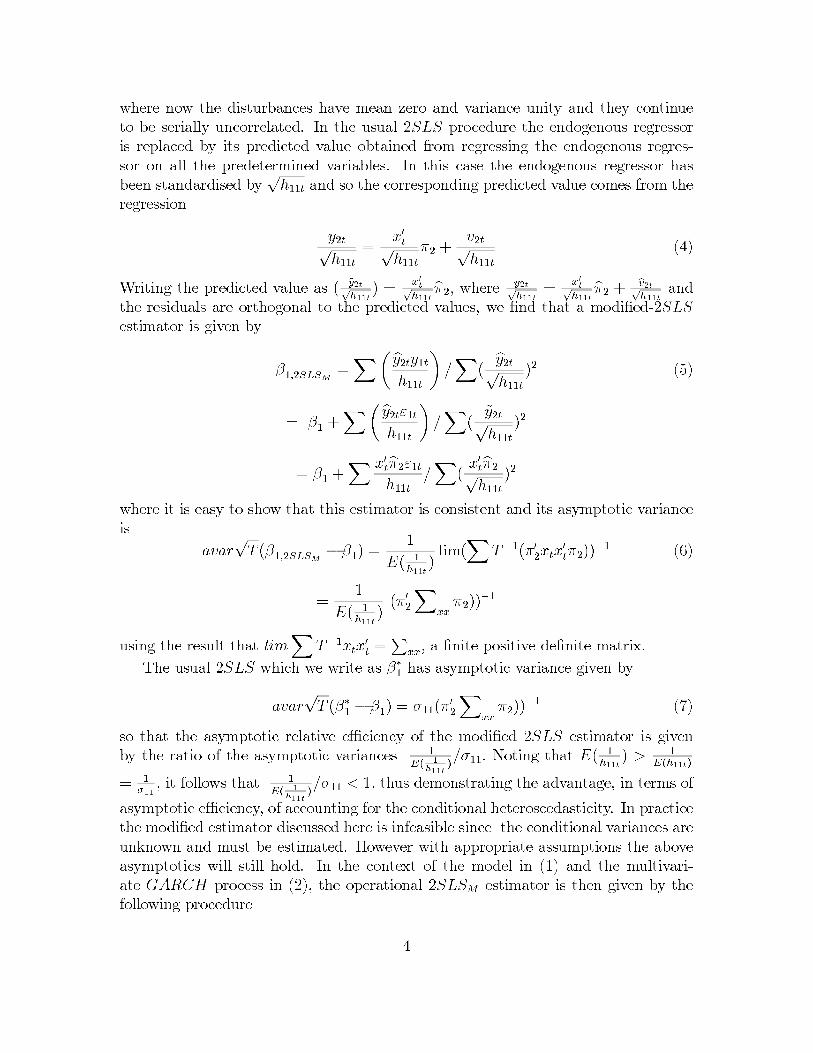
where now the disturbances have mean zero and variance unity and they continueto be serially uncorrelated. In the usual 2SLS procedure the endogenous regressoris replaced by its predicted value obtained from regressing the endogenous regres-sor on all the predetermined variables. In this case the endogenous regressor hasbeen standardised by

√h11t and so the corresponding predicted value comes from the

regression

y2t√h11t

=x′t√h11t

π2 +v2t√h11t

(4)

Writing the predicted value as ( y2t√h11t

) = x′

t√h11t

π2, wherey2t√h11t

= x′

t√h11t

π2 +v2t√h11t

andthe residuals are orthogonal to the predicted values, we find that a modified-2SLSestimator is given by

β1,2SLSM=∑(

y2ty1th11t

)/∑

(y2t√h11t

)2 (5)

= β1 +∑(

y2tε1th11t

)/∑

(y2t√h11t

)2

= β1 +∑ x′tπ2ε1t

h11t/∑

(x′tπ2√h11t

)2

where it is easy to show that this estimator is consistent and its asymptotic varianceis

avar√T (β1,2SLSM

− β1) =1

E( 1h11t

)lim(∑

T−1(π′2xtx′tπ2))

−1 (6)

=1

E( 1h11t

)(π′2∑

xxπ2))

−1

using the result that lim∑

T−1xtx′t =∑

xx, a finite positive definite matrix.

The usual 2SLS which we write as β∗1 has asymptotic variance given by

avar√T (β∗1 − β1) = σ11(π

′2

∑xxπ2))

−1 (7)

so that the asymptotic relative efficiency of the modified 2SLS estimator is givenby the ratio of the asymptotic variances 1

E( 1

h11t)/σ11. Noting that E( 1

h11t) > 1

E(h11t)

= 1σ11

, it follows that 1E( 1

h11t)/σ11 < 1, thus demonstrating the advantage, in terms of

asymptotic efficiency, of accounting for the conditional heteroscedasticity. In practicethe modified estimator discussed here is infeasible since the conditional variances areunknown and must be estimated. However with appropriate assumptions the aboveasymptotics will still hold. In the context of the model in (1) and the multivari-ate GARCH process in (2), the operational 2SLSM estimator is then given by thefollowing procedure

4

STEP 1: Obtain the residuals by running a first round of the traditional 2SLSwithout taking into account the ARCH effects.

STEP 2: Regress these residuals in a multivariate ARCH system to get the esti-mates of h11t.

STEP 3: Regress y2t√h11t

on xt√h11t

to find y2t√h11t

=xtπ2√h11t

which is orthogonal to

v2t√h11t

.

STEP 4: Put y1t√h11t

= β1y2t√h11t

+ε1t√h11t

+v2t√h11t

, whereT∑t=1

y2t√h11t

v2t√h11t

= 0, and

regress y1t√h11t

on y2t√h11t

to obtain

β1,2SLSM

=

⎡⎣ T∑

t=1

⎛⎝ y2t√

h11t

⎞⎠

2⎤⎦−1

T∑t=1

y2t√h11t

y1t√h11t

= β1 +T∑t=1

[y2tε1t

h11t/y22t

h11t

]

It is straightforward to show that it is consistent

p limβ1,2SLSM

= β1+

p lim 1

T

T∑t=1

y2tε1th11t

p lim 1

T

T∑t=1

y22t

h11t

where the numerator goes to zero and the denominator remains finite as T →∞ .While the asymptotic relative efficiency of the 2SLSM procedure has been demon-

strated in the simplest case, the result extends directly to cases where the equationhas more endogenous and exogenous variables. This is discussed again in Section 4.

2.1 Small sample properties of 2SLS and modified-2SLS: ev-

idence from simulations in a simple model

In relation to the finite sample biases, the modified-2SLS procedure proposed in thispaper and the standard 2SLS procedure, are both biased. We give below simulationevidence of how both procedures, can yield estimators with very severe biases in somecircumstances, and bias-correction is often necessary. It is already well known in theliterature that the 2SLS is biased. In relation to the traditional 2SLS, the Nagar(1959) bias approximation for 2SLS in the simple model where only the first equation

5

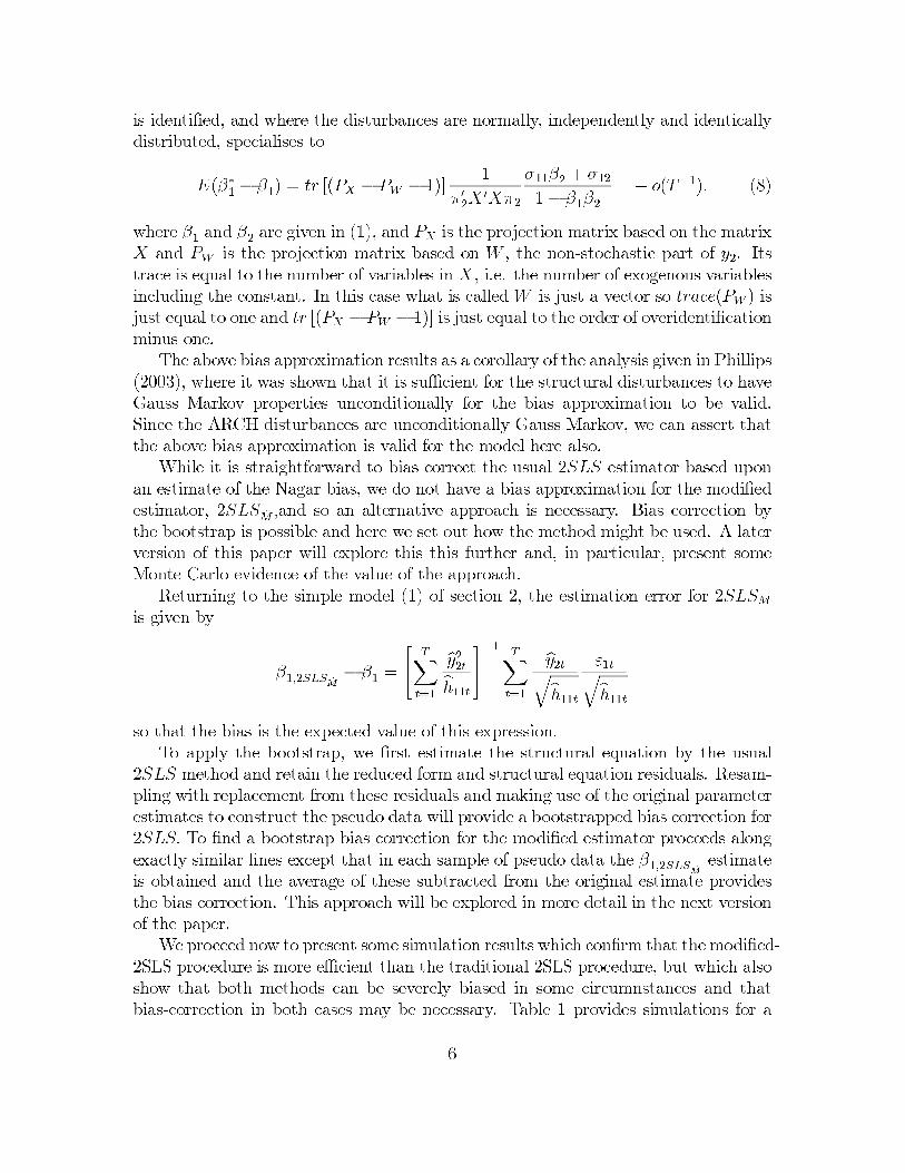
is identified, and where the disturbances are normally, independently and identicallydistributed, specialises to

E(β∗

1− β

1) = tr [(PX − PW − 1)]

1

π′2X ′Xπ2

σ11β2 + σ12

1− β1β2+ o(T−1). (8)

where β1and β

2are given in (1), and PX is the projection matrix based on the matrix

X and PW is the projection matrix based on W , the non-stochastic part of y2. Itstrace is equal to the number of variables in X, i.e. the number of exogenous variablesincluding the constant. In this case what is called W is just a vector so trace(PW ) isjust equal to one and tr [(PX − PW − 1)] is just equal to the order of overidentificationminus one.

The above bias approximation results as a corollary of the analysis given in Phillips(2003), where it was shown that it is sufficient for the structural disturbances to haveGauss Markov properties unconditionally for the bias approximation to be valid.Since the ARCH disturbances are unconditionally Gauss Markov, we can assert thatthe above bias approximation is valid for the model here also.

While it is straightforward to bias correct the usual 2SLS estimator based uponan estimate of the Nagar bias, we do not have a bias approximation for the modifiedestimator, 2SLSM ,and so an alternative approach is necessary. Bias correction bythe bootstrap is possible and here we set out how the method might be used. A laterversion of this paper will explore this this further and, in particular, present someMonte Carlo evidence of the value of the approach.

Returning to the simple model (1) of section 2, the estimation error for 2SLSMis given by

β1,2SLS

ˆM

− β1=

[T∑t=1

y22t

h11t

]−1T∑t=1

y2t√h11t

ε1t√h11t

so that the bias is the expected value of this expression.To apply the bootstrap, we first estimate the structural equation by the usual

2SLS method and retain the reduced form and structural equation residuals. Resam-pling with replacement from these residuals and making use of the original parameterestimates to construct the pseudo data will provide a bootstrapped bias correction for2SLS. To find a bootstrap bias correction for the modified estimator proceeds alongexactly similar lines except that in each sample of pseudo data the β1,2SLS

ˆM

estimateis obtained and the average of these subtracted from the original estimate providesthe bias correction. This approach will be explored in more detail in the next versionof the paper.

We proceed now to present some simulation results which confirm that the modified-2SLS procedure is more efficient than the traditional 2SLS procedure, but which alsoshow that both methods can be severely biased in some circumnstances and thatbias-correction in both cases may be necessary. Table 1 provides simulations for a

6

sample of size 100 based on 5000 replications, and the structure we consider is of theform

Y B +XΓ + ε = 0

where B =

(−1 0.2670.222 −1

)and Γ =

(0 0 0

4.40 0.74 0.13

).

The matrix X contains a first column of ones, while the other two exogenousvariables correspond to normal random variables that have been generated with amean of zero and variance 10. The model has been estimated by 2SLS and 2SLSM .

To represent the behaviour of the disturbances in the structural system we haveselected, for reasons of operational simplicity, the model of Wong and Li (1997) thatfollows the structure

E(ε21t/It−1

)= α0 + α1ε

2

1t−1+ α2ε

2

2t−1

E(ε22t/It−1

)= γ

0+ γ

1ε21t−1

+ γ2ε22t−1

In our simulations we also provide the bias-corrected results of the formula givenin Phillips (2003) for the traditional 2SLS procedure. In the Wong and Li model,in which the disturbances are contemporaneously and serially uncorrelated and ho-moscedastic, the bias approximation will imply σ12 = 0 in the formula given in (8).Thus the bias will then depend directly on β

2and σ11. Results are given in Table 1

below.

Table 1: Simulation results for 2SLS and 2SLSM2SLS ignoring ARCH 2SLSM without ignoring ARCH

bias(β1) s.e.(β1) bias(β1) s.e.(β1)α0 = 0.81, α1 = 0.25, α2 = 0.49 0.002 0.038 0.000 0.029γ0 = 0.64, γ1 = γ2 = 0.49 (0.001) (0.038)α0 = 9, α1 = 0.25, α2 = 0.49 0.014 0.101 -0.012 0.095γ0 = 0.64, γ1 = γ2 = 0.49 (0.009) (0.102)α0 = 0.81, α1 = 0.49, α2 = 0.49 0.005 0.053 0.002 0.048γ0 = 0.64, γ1 = γ2 = 0.49 (0.001) (0.053)α0 = 144, α1 = 0.25, α2 = 0.49 0.130 0.309 -0.099 0.292γ0 = 0.64, γ1 = γ2 = 0.49 (0.077) (0.309)

In brackets we provide the results of the bias-corrected 2SLS using the Phillips(2003) formula. The first interesting result to note, is that indeed the modified-2SLSprocedure is more efficient than the traditional 2SLS procedure. In addition, the2SLSM estimator has a smaller absolute bias while both procedures can have verysevere biases especially when the unconditional variance of the disturbance of the

7

first equation is large. Then, bias correction will be necessary. If the researcher uses2SLS without taking account the ARCH system, then the Nagar bias approximationshould be helpful although it does not account for more than about half of the biasin some scenarios. The bias-corrected estimator performs very well, since apart fromcorrecting the bias, the variance hardly changes. In case the researcher follows oursuggested procedure, Table 1 shows that, although the 2SLSM estimator has less biasthan the traditional 2SLS, bias correction is still necessary and we recommend toapply it through the bootstrap.

Table 1* shows the results when the Engle-Kroner (1995) diagonal representationis used in the variance covariance matrix:

where var (εt/It−1) = Ht =

(h11t h12th21t h22t

)and:

⎛⎝ h11t

h12th22t

⎞⎠ =

⎛⎝ α10

α20

α30

⎞⎠+

⎛⎝ α11 0 0

0 α22 00 0 α33

⎞⎠⎛⎝ ε2

1,t−1

ε1,t−1ε2,t−1ε22,t−1

⎞⎠

Then, it follows that:

E (ε1tε2s/It−1) = α20 + α22ε1t−1ε2s−1, t = s

0 otherwise

E(ε21t/It−1

)= α10 + α11ε

2

1t−1

E(ε22t/It−1

)= α30 + α33ε

2

2t−1

Table 1* also shows the results of the Engle and Kroner (1995) model where wehave used for step 2 of our modified procedure the maximum likelihood estimates ofthe conditional variance of the first disturbance (in theWong and Li (1997) model, theresults are the same regardless of whether we get the estimates from a single equationestimation of the conditional variance of the first disturbance, or if we estimate jointlythe variance covariance matrix).

Table 1*: Simulation results for 2SLS2SLS 2SLSM

bias(β1) s.e.(β

1) bias(β

1) s.e.(β

1)

α10 = 0.81, α20 = 0.25, α11 = 0.49 0.002 0.019 0.001 0.019α30 = 0.64, α22 = α33 = 0.49 (0.001) (0.019)α10 = 9, α1 = 0.25, α2 = 0.49 0.008 0.058 -0.007 0.054α30 = 0.64, α22 = α33 = 0.49 (0.005) (0.058)α10 = 0.81, α20 = 0.25, α11 = 0.98 0.002 0.020 0.000 0.018α30 = 0.64, α22 = α33 = 0.49 (-0.001) (0.019)α10 = 144, α20 = 0.25, α11 = 0.49 0.077 0.221 -0.076 0.217α30 = 0.64, α22 = α33 = 0.49 (0.054) (0.222)

8

3 LIML estimation of a simultaneous equation sys-

tem with conditional heteroscedasticity

In the setting that we have been analysing so far, where only the first of the equa-tions is identified, 2SLS and 3SLS provide the same result. Engle and Kroner (1995)propose to estimate the system more efficiently as well through full information max-imum likelihood or an instrumental variable estimator. In this case, because in ourcontext the second of the equations is not identified, FIML will be equal to LIML. Inthis section we proceed now to consider this estimation method.

Table 2 provides results based on 5000 replications and a sample size of 100, forLIML for the case where we do not take account of the ARCH effects

Table 2: Simulation results for LIMLLIML

bias(β1) s.e.(β

1)

α0 = 0.81, α1 = 0.25, α2 = 0.49 -0.001 0.035γ0= 0.64, γ

1= γ

2= 0.49

α0 = 9, α1 = 0.25, α2 = 0.49 -0.010 0.091γ0= 0.64, γ

1= γ

2= 0.49

α0 = 0.81, α1 = 0.49, α2 = 0.49 -0.005 0.053γ0= 0.64, γ

1= γ

2= 0.49

α0 = 144, α1 = 0.25, α2 = 0.49 -2.812 0.355γ0= 0.64, γ

1= γ

2= 0.49

Care is needed in interpreting these results since it is unclear that estimator mo-ments exist. It is well known that in the classical simultaneous model with normaldisturbances, finite sample LIML estimators do not have moments of any order anda similar non-existence of moments problem may exist here. Indeed extreme valueswere present in the simulations especially for the fourth structure examined. If wewere to consider LIML estimation taking account of the presence of ARCH effectsexplicitly in the LIML procedure, this seems likely to produce a Quasi-LIML estima-tor where the moments would not exist either (considering ARCH effects imply evenfatter tails for the disturbances than under normality). That is why in this paper,when conditional heteroscedasticity is present and we are interested in the structuralparameters, we recommend to use in practice of a 2SLS procedure that takes intoaccount the ARCH effects rather than LIML. Because this type of 2SLS uses the dis-turbance standardised, it should have moments even when the disturbance presentsARCH effects. In Table 2, it is seen that sometimes estimates obtained through LIMLcan be heavily affected by the non-existence of moments mainly when the variance ofthe first disturbance is quite large (a problem which is also documented in Hahn andHausman (2002a) for the case of unconditional correlation when they do not allowfor conditional heteroscedasticity).

9

Table 2* shows the same results for the Engle and Kroner model with the sametype of results.

Table 2*: Simulation results for LIMLLIML

bias(β1) s.e.(β

1)

α10 = 0.81, α20 = 0.25, α11 = 0.49 -0.001 0.019α30 = 0.64, α22 = α33 = 0.49α10 = 9, α20 = 0.25, α11 = 0.49 -0.004 0.056α30 = 0.64, α22 = α33 = 0.49α10 = 0.81, α20 = 0.25, α11 = 0.98 -0.002 0.020α30 = 0.64, α22 = α33 = 0.49α10 = 144, α20 = 0.25, α11 = 0.49 -0.030 0.222α30 = 0.64, α22 = α33 = 0.49

4 Modified 2SLS and 3SLS estimation of a general

simultaneous equation system

So far, we have carried out the analysis in the context of (1) to facilitate the interpre-tation of the analysis. In this section we develop the theoretical approach in a moregeneral setting such as

y1t = β1y2t + x′

1tγ1+ ε1t

y2t = β2y1t + x′2tγ2 + ε2t (9)

In this context, the structural form can be alternatively written

y1t = z´1tα1 + ε1t

y2t = z´2tα2 + ε2t (10)

where

z´1t= (y2t : x1) , z

´

2t= (y1t : x2) .

We shall assume that each equation omits at least two exogenous variables andso is overidentified at least of order 2. As before, we assume that

h11t = E(ε21t

|It−1), h22t = E(ε22t

|It−1), h12t = E(ε1tε2t|It−1) (11)

10

and that the structural disturbances are unconditionally Gauss Markov. Althoughthis is again a simple two-equation model it proves to be completely appropriate forour purposes since all our results can be extended directly to a general simultaneousequation model containing G equations.

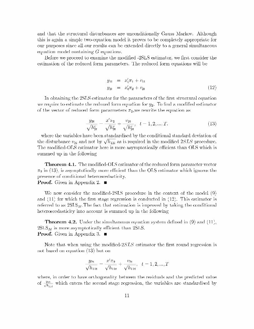
Before we proceed to examine the modified -2SLS estimator, we first consider theestimation of the reduced form parameters. The reduced form equations will be

y1t = x′tπ1 + v1t

y2t = x′tπ2 + v2t (12)

In obtaining the 2SLS estimator for the parameters of the first structural equationwe require to estimate the reduced form equation for y2. To find a modified estimatorof the vector of reduced form pararmeters π2,we rewrite the equation as

y2t√hv2t

=x′π2√hv2t

+v2t√hv2t

, t = 1, 2, ..., T. (13)

where the variables have been standardised by the conditional standard deviation ofthe disturbance v2t and not by

√h11t as is required in the modified 2SLS procedure.

The modified-OLS estimator here is more asymptotically efficient than OLS which issummed up in the following

Theorem 4.1. The modified-OLS estimator of the reduced form parameter vectorπ2 in (13), is asymptotically more efficient than the OLS estimator which ignores thepresence of conditional heteroscedasticity.Proof. Given in Appendix 2.

We now consider the modified-2SLS procedure in the context of the model (9)and (11) for which the first stage regression is conducted in (12). This estimator isreferred to as 2SLSM .The fact that estimation is improved by taking the conditionalheteroscedasticity into account is summed up in the following

Theorem 4.2. Under the simultaneous equation system defined in (9) and (11),2SLSM is more asymptotically efficient than 2SLS.Proof. Given in Appendix 3.

Note that when using the modified-2SLS estimator the first round regression isnot based on equation (13) but on

y2t√h11t

=x′π2√h11t

+v2t√h11t

, t = 1, 2, ..., T

where, in order to have orthogonality between the residuals and the predicted valueof y2t√

h11twhich enters the second stage regression, the variables are standardised by

11

the conditional standard deviation of the structural disturbance and not the reducedform disturbance. Although the resulting estimator of π2 is not explicitly used, it isof interest to compare its asymptotic efficiency with that which results in Theorem4.2. We do this in the following

Theorem 4.3. If the alternative modified-OLS estimator of π2 which results fromthe regression in (13) is used to construct an alternative modified 2SLS estimator, theresulting estimator may be more or less asymptotically efficient than the estimatorin Theorem 4.2.Proof. Given in Appendix 4.

We know from the standard literature that 3SLS is always more efficient than2SLS when the equations are overidentified and the disturbances are contemporane-ously correlated. Thus, in the model of this section, 3SLS is more asymptoticallyefficient than 2SLS and so might be preferred. However, we shall see that it too isless asymptotically efficient than a modified-3SLS (3SLSM) procedure. This 3SLSMprocedure will imply in practical applications following a similar procedure than thetraditional 3SLS, but where again we standardise by the conditional variances of thestructural disturbances.

First consider again the structural equations

y1t = β1y2t + x′

1tγ1+ ε1t

y2t = β2y1t + x′

2tγ2 + ε2t, t = 1, 2, ......, T. (14)

We shall write the system as

(y1y2

)=

(Z1 00 Z2

)(α1

α2

)+

(ε1ε2

)

where Zi = (yi : Xi), αi = ( βi

γ ′

i)′, i = 1, 2.

Premultiplying byX ′,the matrix which contains all the exogenous variables, yieldsthe system

(X ′y1X ′y2

)=

(X ′Z1 00 X ′Z2

)(α1

α2

)+

(X ′ε1X ′ε2

)

where the covariance matrix of the transformed disturbances is

E

(X ′ε1X ′ε2

)(X ′ε1X ′ε2

)′

=

(σ11X

′X σ12X′X

σ21X′X σ22X

′X

)

= Σ⊗ (X ′X)

12

where Σ =

(σ11 σ12

σ21 σ22

).

Applying GLS to this system yields the 3SLS-GLS estimator(σ11Z1PXZ1 σ12Z1PXZ2

σ21Z2PXZ1 σ22Z2PXZ2

)−1(

σ11Z1PXy1 + σ12Z1PXy2σ22Z2PXy2 + σ21Z2PXy1

)(15)

where PX = X(X ′X)−1X ′.To obtain the modified 3SLS estimator we first define two diagonal matrices given

by

Λ1

2

1=

⎛⎜⎜⎜⎝

1√h111

0 ... 0

0 1√h112

... 0

... ... ... 00 0 ... 1√

h11T

⎞⎟⎟⎟⎠ ,Λ

1

2

2=

⎛⎜⎜⎜⎝

1√h221

0 ... 0

0 1√h222

... 0

... ... ... 00 0 ... 1√

h22T

⎞⎟⎟⎟⎠

These matrices are used to standardise the variables in the system so that thesystem becomes(

Λ1

2

1y1

Λ1

2

2y2

)=

(Λ

1

2

1Z1 0

0 Λ1

2

2Z2

)(α1

α2

)+

(Λ

1

2

1ε1

Λ1

2

2ε2

)

Premultiplying through the first set of equations by X ′Λ1

2

1and the second by

X ′Λ1

2

2yields(

X ′Λ1y1X ′Λ2y2

)=

(X ′Λ1Z1 0

0 X ′Λ2Z2

)(α1

α2

)+

(X ′Λ1ε1X ′Λ2ε2

)

where the covariance matrix of the transformed disturbances is

E

(X ′Λ1ε1X ′Λ2ε2

)(X ′Λ1ε1X ′Λ2ε2

)′= E

(X ′Λ1ε1ε

′1Λ1X X ′Λ1ε1ε

′2Λ2X

X ′Λ2ε2ε′1Λ1X X ′Λ2ε2ε

′2Λ2X

)

which in large samples is approximately equal to

= ΣM ⊗ (X ′X)

where

ΣM =

⎛⎝ E( 1

h11t) −ρ

12

√E( 1

h11t)E( 1

h22t)

−ρ12

√E( 1

h11t)E( 1

h22t) E( 1

h22t)

⎞⎠ with ρ

12=

σ12√σ11√σ22

.

(16)Applying GLS to this transformed system will yield the modified-3SLS-GLS esti-

mator

13

(α1

α2

)=

⎛⎝ E( 1

h11t)Z1Λ1PxΛ1Z1 −ρ

12

√E( 1

h11t)E( 1

h22t)Z1Λ1PxΛ2Z2

−ρ12

√E( 1

h11t)E( 1

h22t)Z2Λ2PxΛ1Z1 E( 1

h22t)Z2Λ2PxΛ2Z2

⎞⎠−1

×

⎛⎝ E( 1

h11t)Z1Λ1PxΛ1y1 − ρ

12

√E( 1

h11t)E( 1

h2t)Z1Λ1PxΛ2y2

−ρ12

√E( 1

h11t)E( 1

h22t)Z2Λ2PxΛ1y1 + E( 1

h22t)Z2Λ2PxΛ2y2

⎞⎠

We may now state the following

Theorem 4.4. Under the simultaneous equation system defined in (9) and (11),3SLSM is more asymptotically efficient than 3SLS.Proof. Given in Appendix 5.

The results in Theorems 4.2 and 4.4 are given in the context of the estimators2SLSM and 3SLSM both of which are non-operational since the standardising con-ditional standard deviations are unknown. However, the conditional standard de-viations can be consistently estimated from the residuals obtained following firstround estimation so that operational versions are readily found. These operationalestimators will have the same asymptotic distribution as the 2SLSM and 3SLSMcounterparts. This matter will be considered further in the next version of the paper.

5 Simultaneous equations and weak instruments

under conditional heteroscedasticity

It is quite well known (see for example Stock, Wright and Yogo (2002)) that thereexists a concentration parameter (µ) such that, if we consider a single endogenousregressor with no included exogenous variables such as

y1 = βy2 + u

y2 = Xπ + v

thenµ2 = π′XXπ/σ2

v

is a unitless measure of the strengh of the instruments.So far in this paper, we have shown that increasing conditional heteroscedasticity

increases the unconditional variance and hence, the denominator in µ. In this sectionof the paper we are going to simulate again the same model as before, but reducingthe values of the π coefficients.

14

The structure we consider now is of the form:

Y B +XΓ + ε = 0

where B =

(−1 0.267

0.222 −1

)and Γ =

(0 0 0

1.47 0.246 0.043

).

Table 3: Simulation results for 2SLS and 2SLSM2SLS 2SLSM

bias(β1) s.e.(β

1) bias(β

1) s.e.(β

1)

α0 = 0.81, α1 = 0.25, α2 = 0.49 0.017 0.107 0.002 0.099γ0= 0.64, γ

1= γ

2= 0.49 (0.013) (0.108)

α0 = 9, α1 = 0.25, α2 = 0.49 0.080 0.248 -0.078 0.233γ0= 0.64, γ

1= γ

2= 0.49 (0.051) (0.248)

α0 = 0.81, α1 = 0.49, α2 = 0.49 0.037 0.149 0.004 0.125γ0= 0.64, γ

1= γ

2= 0.49 (-0.002) (0.150)

α0 = 144, α1 = 0.25, α2 = 0.49 0.270 0.420 -0.236 0.416γ0= 0.64, γ

1= γ

2= 0.49 (0.173) (0.421)

Table 3*: Simulation results for 2SLS2SLS 2SLSM

bias(β1) s.e.(β1) bias(β1) s.e.(β1)α10 = 0.81, α20 = 0.25, α11 = 0.49 0.018 0.058 -0.017 0.056α30 = 0.64, α22 = α33 = 0.49 (0.014) (0.056)α10 = 9, α20 = 0.25, α11 = 0.49 0.074 0.165 -0.065 0.160α30 = 0.64, α22 = α33 = 0.49 (0.054) (0.166)α10 = 0.81, α20 = 0.25, α11 = 0.98 0.021 0.056 -0.013 0.054α30 = 0.64, α22 = α33 = 0.49 (-0.017) (0.060)α10 = 144, α20 = 0.25, α11 = 0.49 0.639 0.454 -0.638 0.416α30 = 0.64, α22 = α33 = 0.49 (0.427) (0.533)

Table 4: Simulation results for LIML

LIML

bias(β1) s.e.(β

1)

α0 = 0.81, α1 = 0.25, α2 = 0.49 0.022 0.096γ0= 0.64, γ

1= γ

2= 0.49

α0 = 9, α1 = 0.25, α2 = 0.49 0.422 0.243γ0= 0.64, γ

1= γ

2= 0.49

α0 = 0.81, α1 = 0.49, α2 = 0.49 0.035 0.120γ0= 0.64, γ

1= γ

2= 0.49

α0 = 144, α1 = 0.25, α2 = 0.49 -2.416 0.888γ0= 0.64, γ

1= γ

2= 0.49

15

Table 4*: Simulation results for LIMLLIML

bias(β1) s.e.(β

1)

α10 = 0.81, α20 = 0.25, α11 = 0.49 -0.002 0.057α30 = 0.64, α22 = α33 = 0.49

α10 = 9, α20 = 0.25, α11 = 0.49 -0.022 0.160α30 = 0.64, α22 = α33 = 0.49

α10 = 0.81, α20 = 0.25, α11 = 0.98 -0.003 0.057α30 = 0.64, α22 = α33 = 0.49

α10 = 144, α20 = 0.25, α11 = 0.49 -0.200 0.607α30 = 0.64, α22 = α33 = 0.49

We observe that, indeed, the biases increase a lot in this new situation, and theformula given in Phillips (2003) provides again a good bias-corrected 2SLS estimator.2SLSM is again more effiicient than 2SLS and the bias in absolute terms is smalleras well. In relation to LIML, we experience many problems with outliers and carefulanalysis must be followed in relation to Table 4. Again, we advise the use of 2SLSMin case any bias-corrected mechanism is applied. Again tables 3* and 4* correspondto the Engle and Kroner (1995) diagonal representation.

6 Conclusions

In this paper we have studied simultaneous equation systems and how 2SLS and3SLS behave in this framework. First we have shown, that if structural disturbancesfollow ARCH processes the reduced form disturbances do not unless some strongconditions are imposed. We have also proposed modified 2SLS and 3SLS proceduresthat are more asymptotically efficient than their traditional counterparts. When theresearcher is interested in estimating the structural parameters, we recommend to useour modified procedures instead of LIML (or FIML) where the existence of extremevalues can produce misleading results in practice. This is due to the non-existence ofmoments, which is even more evident in the context of conditional heteroscedasticywhere the tails are fatter than in the regular case. We have also showed throughMonte Carlo simulations how all the procedures can produce important biases, mainlywhen the disturbances are very volatile, and we provide bias mechanisms to apply inpractice. When we analyse the weak instruments case, the conclusions of this paperare even more emphasized.

16

7 Appendices

Appendix 1

Proof. of Proposition 2.1.

In this appendix we show that if the structural disturbances follow a multivariate-ARCH(1) process, the reduced form disturbances may also follow a multivariate-ARCH(1) process but only under strict conditions. To show this we suppose that thedisturbances in (1) follow, for example, a diagonal representation (for simplicity, butwithout loss of generality)

h11t = E(ε21t|It−1) = α0 + α1ε21t−1, h22t = E(ε22t|It−1) = θ0 + θ1ε

22t−1,

h12t = E(ε1tε2t|It−1) = λ1 + λ2ε1,t−1ε2,t−1

Note that v2t, the reduced form disturbance in the second equation, is defined by

v2t =(β2ε1t + ε2t)

1− β1β2

, β1β2 �= 1.

Also E(v22t) =β22σ11+2β2σ12+σ22

(1−β1β2)2 , while the conditional variance is given by

E(v22t|It−1) =β22

(1 − β1β2)2(α0 + α1ε

21,t−1) +

2β2

(1 − β1β2)2(λ1 + λ2ε1,t−1ε2,t−1)

+1

(1 − β1β2)2(θ0 + θ1ε

22,t−1)

=β22

(1 − β1β2)2h1t +

2β2

(1− β1β2)2h12t +

1

(1− β1β2)2h2t

Next we have v22t−1 =β22ε21t−1

+2β2ε1,t−1ε2,t−1+ε2

2,t−1

(1−β1β2)2

, from which it is apparent that it

is not possible to write E(v22t|It−1) = φ1 + φ2v22t−1 for some φ1, φ2 unless restrictions

are placed on the original ARCH(1) processes. In particular, for v2t to follow anARCH(1) process of the usual kind the component ARCH processes will have tohave the same variance parameter. Clearly this is a severe restriction to impose, andthis proves the proposition.

Similarly we may show that the 2× 1 vector v =

[v1tv2t

]has a conditional covari-

ance matrix given by

E(vv′|It−1) =

[hv1t hv

12t

hv21t hv

2t

], where

hv1t =

β21

(1 − β1β2)2h2t +

2β1

(1− β1β2)2h12t +

1

(1 − β1β2)2h1t

17

hv12t = hv21t = β2h1t + (1 + β1β2)h12t + β1h2t

hv2t =β22

(1 − β1β2)2h1t +

2β2

(1− β1β2)2h12t +

1

(1 − β1β2)2h2t

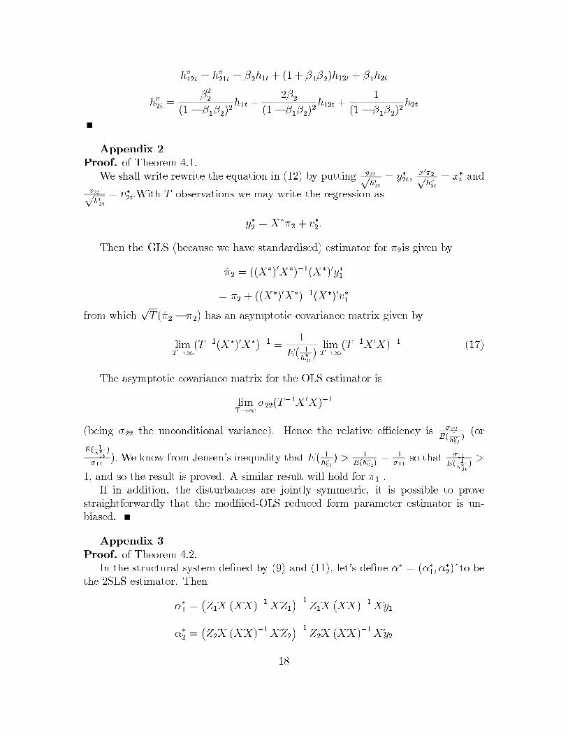
Appendix 2

Proof. of Theorem 4.1.We shall write rewrite the equation in (12) by putting y2t√

hv2t

= y∗2t,x′π2√hv2t

= x∗t andv2t√hv2t

= v∗2t.With T observations we may write the regression as

y∗2 = X∗π2 + v∗2.

Then the GLS (because we have standardised) estimator for π2is given by

π2 = ((X∗)′X∗)−1(X∗)′y∗1

= π2 + ((X∗)′X∗)−1(X∗)′v∗1

from which√T (π2 − π2) has an asymptotic covariance matrix given by

limT→∞

(T−1(X∗)′X∗)−1 =1

E( 1hv2t

)limT→∞

(T−1X ′X)−1 (17)

The asymptotic covariance matrix for the OLS estimator is

limT→∞

σ22(T−1X ′X)−1

(being σ22 the unconditional variance). Hence the relative efficiency is σ22

E( 1

hv2t

)(or

E( 1

hv1t

)

σ11).We know from Jensen’s inequality that E( 1

hv2t

) > 1E(hv

2t)= 1

σ11so that σ11

E( 1

hv2t

)>

1, and so the result is proved. A similar result will hold for π1 .If in addition, the disturbances are jointly symmetric, it is possible to prove

straightforwardly that the modfiied-OLS reduced form parameter estimator is un-biased.

Appendix 3

Proof. of Theorem 4.2.In the structural system defined by (9) and (11), let’s define α∗ = (α∗1, α

∗

2) to bethe 2SLS estimator. Then

α∗1 =(Z1X (XX)−1

XZ1

)−1Z1X (XX)−1

Xy1

α∗2 =(Z2X (XX)−1

XZ2

)−1Z2X (XX)−1

Xy2

18

Analysing the distrubution of√T (α∗

1− α1), the asymptotic covariance matrices

are given by

avar(√

T (α∗1− α1)

)= σ11p limT

(Z1X (XX)−1 XZ1

)−1avar

(√T (α∗

2− α2)

)= σ22p limT

(Z2X (XX)−1 XZ2

)−1where σ11 and σ22 are the two unconditional variances of the structural disturbances.

In the case of our modified-2SLS procedure, let’s define α = (α1, α2) to be the

modified-2SLS estimator. Then, put

Λ1

2

1=

⎛⎜⎜⎜⎝

1√h111

0 ... 0

0 1√h112

... 0

... ... ... 00 0 ... 1√

h11T

⎞⎟⎟⎟⎠ ,Λ

1

2

2=

⎛⎜⎜⎜⎝

1√h221

0 ... 0

0 1√h222

... 0

... ... ... 00 0 ... 1√

h22T

⎞⎟⎟⎟⎠

We may show that

α1 =(Z1Λ1X(X ′Λ1X)−1X ′Λ1Z1

)−1Z1Λ1X(X ′Λ1X)−1X ′Λ1y1

α2 =(Z2Λ2X(X ′Λ2X)−1X ′Λ2Z2

)−1Z2Λ2X(X ′Λ2X)−1X ′Λ2y2

The asymptotic covariance matrix of α1 is

avar(√

T (α1 − α1

)) = p limT

(Z1Λ1X(X ′Λ1X)−1X ′Λ1Z1

)−1=

1(E(

1

h11t

))p lim( 1

TZ1PxZ1

)−1

Using Jensen’s inequality

E

(1

h11t

)>

1

E (h11t)

E (h11t) = σ11⇒ E

(1

ht11t

)>

1

σ11

Thus we have proved that this non-operational 2SLSM is more asymptotically

efficient than 2SLS. The same would hold for α2.

Appendix 4

Proof. of Theorem 4.3.

Suppose we use the modified OLS estimator of π2 to construct the modified 2SLSestimator. We now have the equation:

y∗∗1

= β1y∗∗2+ ε∗∗

1+ β

1v∗∗2.

19

The usual situation does not apply here: y∗∗2

= X∗∗π2 is not orthogonal to thesecond component of the error term β

1v2. However, the implied 2SLS estimator will

still beβ1 = [(π2)

′(X∗∗)′X∗∗π2}−1(π2)′(X∗∗)′y∗∗1

= β1+ [(π2)

′(X∗∗)′X∗∗π2}−1(π2)′(X∗∗)′(ε∗∗

1+ β

1v∗∗2) =

β1+ [(π2)

′(X∗∗)′X∗∗π2}−1(π2)′(X∗∗)′ε∗∗

1+ [(π2)

′(X∗∗)′X∗∗π2}−1(π2)′(X∗∗)′β

1v∗∗2)

Then as T →∞√T ( β

1− β

1) ∼ [(π2)

′1

T(X∗∗)′X∗∗π2]

−1(π2)′T−1/2(X∗∗)′(ε∗∗

1+ β

1v∗∗2)

which has asymptotic covariance matrix given by

avar(√T ( β

1− β

1)) = var(ε∗∗

1t + β1v∗∗2t )

1

(E( 1

hw11t

))limT→∞

[(π2)′1

T(X ′X)π2]

−1

which may be more or less asymptotically efficient than the usual 2SLSM dependingon whether or not var(ε∗∗

1t + β1v∗∗

2t ) � 1.

Appendix 5

Proof. of Theorem 4.4.In the structural system defined by (9) and (11), let α∗∗ = (α∗∗

1, α∗∗

2) to be the

3SLS estimator. Then, the asymptotic covariance matrix will be given by

avar

(√T

(α∗∗1− α1

α∗∗2− α2

))= p limT

(σ11Z1PXZ1 σ12Z1PXZ2

σ21Z2PXZ1 σ22Z2PXZ2

)−1

= p limT

(1

1−ρ212

1

σ11Z1PxZ1 − σ12

σ11σ22

1

1−ρ212

Z1PxZ2

− σ12σ11σ22

1

1−ρ212

Z2PxZ11

1−ρ212

1

σ22Z2PxZ2

)−1

= (1− ρ212) p limT

(1

σ11Z1PxZ1 − σ12

σ11σ22Z1PxZ2

− σ12σ11σ22

Z2PxZ11

σ22Z2PxZ2

)−1a result that makes use of the fact that the unconditional variance/covariance matrixcan be written as

Σ−1 =

(σ11 σ12

σ21 σ22

)=

1

1− ρ212

(1

σ11− σ12

σ11σ22− σ12σ11σ22

1

σ22

)Here we have defined the unconditional correlation coefficient as ρ

12. On the

other hand, if we define the modified-3SLS estimator by ˜α =(˜α1, ˜α2

), then, the

20

asymptotic covariance matrix is given by

avar

(√T

( ˜α1 − α1˜α2 − α2

))

= (1 − ρ212)p limT

⎛⎝ 1E( 1

h1t)Z1Λ1PxΛ1Z1

−ρ12√

E( 1

h1t)E( 1

h2t)Z1Λ1PxΛ2Z2

−ρ12√E( 1

h1t)E( 1

h2t)Z2Λ2PxΛ1Z1

1E( 1

h2t)Z2Λ2PxΛ2Z2

⎞⎠−1

= (1 − ρ212)p limT

⎛⎝ E( 1h1t

)Z1PXZ1 −ρ12√E( 1

h1t)E( 1

h2t)Z1PXZ2

−ρ12√E( 1

h1t)E( 1

h2t)Z2PXZ1 E( 1

h2t)Z2PXZ2

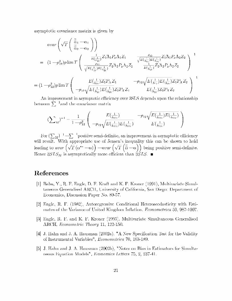
⎞⎠−1

An improvement in asymptotic efficiency over 3SLS depends upon the relationshipbetween

∑−1and the covariance matrix

(∑

M)−1 =

1

1− ρ212

⎛⎝ E( 1h11t

) −ρ12√E( 1

h11t)E( 1

h22t)

−ρ12√E( 1

h11t)E( 1

h22t) E( 1

h22t)

⎞⎠For (

∑M)−1−

∑−1positive semi-definite, an improvement in asymptotic efficiency

will result. With appropriate use of Jensen’s inequality this can be shown to hold

leading to avar(√

T (α∗∗ − α))− avar

(√T(˜α− α

))being positive semi-definite.

Hence 3SLSM is asymptotically more efficient than 3SLS.

References

[1] Baba, Y., R. F. Engle, D. F. Kraft and K. F. Kroner (1991), Multivariate Simul-taneous Generalised ARCH, University of California, San Diego: Department ofEconomics, Discussion Paper No. 89-57.

[2] Engle, R. F. (1982), Autoregressive Conditional Heteroscedasticity with Esti-mates of the Variance of United Kingdom Inflation. Econometrica 50, 987-1007.

[3] Engle, R. F. and K. F. Kroner (1995), Multivariate Simultaneous GeneralisedARCH, Econometric Theory 11, 122-150.

[4] J. Hahn and J. A. Hausman (2002a), "A New Specification Test for the Validityof Instrumental Variables", Econometrica 70, 163-189.

[5] J. Hahn and J. A. Hausman (2002b), "Notes on Bias in Estimators for Simulta-neous Equation Models", Economics Letters 75, 2, 237-41.

21

[6] J. Hahn and J. A. Hausman (2003), "Weak Instruments: Diagnosis and Curesin Empirical Econometrics", American Economic Review, 93, 2, 118-125.

[7] J. Hahn, J. A. Hausman and G. Kuersteiner (2002), "Estimation with WeakInstruments: Accuracy of Higher Order Bias and MSE Approximations", MITWorking Paper.

[8] Harmon, R. (1988), The simultaneous EquationsModel with Generalised Autore-gressive Conditional Heteroscedasticity: the SEM-GARCH Model, WashingtonD. C.: Board of Governors of the Federal Reserve System, International FinanceDiscussion Papers, No. 322.

[9] Hausman, J. A. (1983), "Specification and Estimation of Simultaneous EquationModels" in Griliches, Zvi and Intriligator, Michael, eds., Handbook of Economet-

rics, Volume 1, Amsterdam : North Holland.

[10] Nagar, A. L. (1959), The Bias and Moment Matrix of the General k-class Esti-mators of the Parameters in Simultaneous Equations. Econometrica 27, 575-95.

[11] Phillips, G. D. A. (2003), ”Nagar-type moment approximations in simultane-ous equation models: some further results. Paper presented at Contributionsto Econometric Theory: Conference in Memory of Michael Magdalinos, AthensNovember 2003.

[12] Stock, J. H., J. H. Wright and M. Yogo (2002), A Survey of Weak Instrumentsand Weak Identification in Generalized Method of Moments, Journal of Businessand Economic Statistics 20, 4, 518-529.

[13] Wong, H. and W. K. Li (1997), On a Multivariate Conditional HeteroscedasticModel, Biometrika 84, 1, 111-123.

22