Using Regression Estimation to Calculate Effective Load Carrying Capacity of Renewable Resources

7/30/2019 Using Regression Estimation to Calculate Effective Load Carrying Capacity of Renewable Resources

http://slidepdf.com/reader/full/using-regression-estimation-to-calculate-effective-load-carrying-capacity-of 1/17

1

Using Regression Estimation to Calculate Effective Load Carrying

Capacity of Renewable Resources

Paul Nelson and Justin Kubassek 1

Southern California Edison Company

Presented at the Rutgers 26th Annual Western Conference

Monterey, California

June 20, 2013

Abstract: California’s ambitious Renewables Portfolio Standard (RPS)

mandates that 33% of its energy must come from renewable resources by

2020. To achieve this policy goal, a significant amount of wind and solar

resources are being built. As the amount of renewable resources grows, sohas the debate over their contribution to system reliability of these

renewable intermittent resources. Effective Load Carrying Capacity

(ELCC) is one metric for measuring a resource’s contribution to systemreliability and has historically been calculated using reliability simulation

models. However, this approach to calculating ELCC is time consumingfor jurisdictions that have annual resource adequacy filings to regulators.

The authors explore a method to calibrate a regression approach usingresults from reliability modeling for use in annual ELCC determination for

resource adequacy proceedings.

1. Introduction

In order to provide reliable service, the utility needs to know the amount of generation

capacity that can be depended upon to meet future peak demands. Further, utility

planners must balance the cost of additional generation against the value customers placeon the additional reliability provided by the additional generation. A typical reliability

standard for utility planners and regulators is that, on average, generation is be able tomeet load in all but one day out of every ten years ( 1 in 10).

1 This paper presents ongoing work, so the descriptions of modeling methods herein are subject to revision.

The opinions contained in this paper are the authors’ own and do not necessarily reflect the views of

Southern California Edison Company.



2

Just how much generation is needed to meet this 1 in 10 standard, however, depends on

the reliability of the generation fleet as well as the volatility and behavior of customer

demand. In California, the Public Utilities Commission (CPUC) has established that totalgeneration should be between 115% and 117% of expected annual peak load based on a

one-day-in-ten-years criterion. Further, the CPUC requires that load-serving entities

under its jurisdiction demonstrate on a monthly basis that they either own or have procured commitments from enough generation to meet 115% of expected peak load for the prompt month.

Importantly, these benchmarks were derived when most of the generation system

consisted of non-intermittent generation that could be reasonably relied upon to provide

their maximum rated output at any time. However, as intermittent resources, such aswind and solar, become increasingly important elements of the generation system, utility

planners and regulators must seriously ask, “How much should a given resource count

toward meeting these mega-watt targets?” Understanding the coincidence of resource

availability and system stress periods is essential to answering this question, as not allresources have the same value in providing reliability. For instance, a resource that can

produce 100% of its peak output only from midnight to 6am would likely have minimal

value to a system serving load that peaks at 3pm. On the other hand, a resource that is

always available would contribute much more to system reliability. The contribution thateach resource provides to system reliability can be measured by its effective load

carrying capacity (ELCC), which is defined as the amount of load that an amount of

generating capacity can support without decreasing system reliability. While it may bereasonable to assume that a natural-gas fired plant has an ELCC near its maximum rated

capacity, the same is not true for intermittent resources like wind and solar with highly

variable fuel sources. Developing and implementing a method that can estimate the

ELCC for wind and solar resources is of paramount importance to ensuring that anappropriate level of generation system reliability is maintained.

Currently, two approaches are employed to calculate the contribution of intermittent

resources to generation system reliability: (1) the reliability modeling method (2) the

proxy methods. Both methods present opportunities and challenges in recurringregulatory settings. Reliability modeling is considered the benchmark approach but is

time-consuming and resource intensive. Using this approach, it is difficult to assess

numerous individual projects on an annual basis. In contrast, proxy methods, which rely

on simple statistics, can be used to quickly assign value to many projects each year.However, a proxy may dramatically misrepresent a resource’s true value without

appropriate benchmarking. Further, the simplistic framework behind established proxy

methods may miss important relationships between the underlying distribution of a

resource’s performance and the changing needs of the electricity system.

Through this paper, the authors present a new approach that can accurately approximatethe output of the reliability modeling method, yet can be applied on a project-by-project

basis in a similarly simple manner as the proxy method. For this reason, the authors refer

to this approach as “the hybrid approach.” The approach utilizes the results of reliabilitymodeling to develop a formula that can be applied to many projects each year. The



3

approach allows many variables to be assessed and would only require updating on a

period basis as system conditions change.

The rest of this paper is outlined as follows. Section 2 reviews existing methods. Section

3 describes the reliability model the authors developed. Section 4 and 5 describe the

process the authors followed to develop the hybrid approach using the reliability model,and Section 6 concludes.

2. Review of Existing Methods

A. Reliability Modeling

A traditional method of determining ELCC is to use a reliability model which directlyincorporates uncertainty in both load and the availability of existing generation resource

mix. The model will generally use Monte Carlo or other stochastic methods to generate

various possible outcomes of load and resource availability. The model, with a

distribution of loads and resources, is able to calculate the electric system’s loss of load

expectation (LOLE), which is a measurement of how likely the system is to have anoutage due to insufficient generation. Hourly reliability models are common and can be

used to capture time of day or seasonal likelihood that load is likely to be unserved.Further, the models capture fleet forced outage and maintenance characteristics. The

LOLE calculation considers expected capacity less expected load for every hour as well

as volatility around each. This interaction is important because it is possible to have

significant LOLE not during the annual peak but during a period of expected hot weather when resources are on maintenance. The advantage of this approach is its ability to

directly consider the interaction between load and resource uncertainty throughout the

year enabling the researcher to assess a resource’s contribution to reliability withoutmaking any a priori assumptions regarding which times are more or less likely to

experience loss of load. Simply put, there is no requirement to make assumptionsregarding the time of day or season when resources improve reliability as the results will

provide that information. For this reason, reliability modeling is the benchmark assessment of a resource’s ELCC.

Calculating the ELCC using modeling involves the following steps:

1. Determine the reliability level of the existing system and calculate the amount of

loss of load expectation (LOLE).

2. Add the test resource (i.e. a solar unit) to the system, and calculate LOLE.

a. If LOLE does not change, then the resource does not improve system

reliability and will have an ELCC of zero.

b. If LOLE is lower, go to step 3.

3. Increase load until LOLE is the same value obtained in step 1.

4. The amount of load added is the ELCC of the resource.



4

Unfortunately, reliability modeling is resource intensive and requires many assumptions

about loads and resources to be made upfront. While a utility can perform these

calculations for their system, it becomes more difficult for a very large system withnumerous renewable resource types and locations. For example, the ELCC of a wind

turbine is dependent on its technology and location. This presents a challenge to

calculate ELCCs for numerous projects that vary by location on a frequent basis. For example, California’s Resource Adequacy program requir es values for each generation project on a monthly basis for the entire state.

To be able to use reliability modeling on an annual basis, the process would need to be

simplified by grouping technology and locations together into to a technology/location

class average. This result is an ELCC is that is based upon a group average. This posesa problem because individual project performance would not be assessed in the annual

accounting process.

To summarize, the reliably model approach offers the opportunity to calculate accurateELCC. However, it requires significant modeling efforts to implement. To reduce the

modeling effort it would likely require class averaging of projects, which could reducethe measurement of individual project performance.

B. Proxy Methods

A simplified approach for determining a resource’s contribution to system reliabilityrelies on proxy ELCC calculations. A typical approach calculates the resource’s outputduring specific time periods when the system is likely to need resources, such as the

afternoon in the summer or the evening in winter. This assumes that additional resources

are most beneficial during these time periods. The advantage of the proxy method is theease of calculation and the incorporation of the resource’s actual perf ormance in the

calculation. Projects that perform better during the test hours obtain a higher capacityvalue than units with less performance. Further, if the time period of system stress is

known, then a reasonable proxy can be obtained.

However, these methods tend to be biased toward typical, or most likely, occurrences of hot weather, which do not necessarily capture or adequately weight potential events, such

as a hot weather event during times of typically high maintenance. Proxy methods ignore

the resource availability assumptions which are included in the reliability modelapproach. Additionally, most of the proxy methods reviewed by the authors tend to treat

all hours the same in terms of reliability need. For example, for a summer month, not all

days from noon-6pm are system stress hours. A typical heat wave may occur for a week

or two, but eventually the weather returns to average levels. The proxy methods alsotend to treat the months equally as well, and there may be differences between June and

September.

Furthermore, increasing penetrations of solar, which is available only during certain

hours of the day, changes the reliability of the system in a way not captured by proxy

methods developed prior to these changes in resource mix. At some point addingadditional solar does not improve daytime reliability because all the LOLE during the



5

hours of high solar generation eliminated. The time period when a resource can improve

system reliability has changed. In this case, the time periods used in the proxy method

need to be revised.2

The proxy methods used by California and Southwest Power are described below.

California

In April, 2008, the Energy Division of the California Public Utility Commission (CPUC)

issued its 2007 Resource Adequacy Report which showed that the a method of a simple

average production overstated the available capacity of wind resources during peak demand periods.

3The report documented that the output of wind was negatively

correlated during period of hot weather, therefore also high loads, than compared to

normal periods of weather. This had the impact of overstating the contribution of wind

resources to meet peak load on those very hot days. Therefore the CPUC adopted areplacement method called the exceedance methodology which is the quantity of output

achieved 70 percent of the time4

during a specified period the hours and using three years

of historical operation data.5 For new units without historical data, then data based upontechnology and regional averages are blended into the calculation. Many organizations

use similar methods such as PJM ISO, NYISO, New England ISO and each ISO uses

time periods reflecting their unique load patterns.

While this approach does the advantage of simplicity and ease of calculate, is does have

another drawback in that all hours during are summer time on-peak period are treatedequally. The fact is LOLE will only occur in some of those time periods because the

weather was average or below average for the summer. LOLE is more likely to occur

during the very hot periods.

Southwest Power Pool

The Southwest Power Pool uses historical output based upon the top 10 percent of load

hours for each month. The resource’s output during the top 10% of the hours is rankedfrom highest to lowest, and then the value exceeded 85% percent of the time is selected.

This method takes into account the higher load hours in the month and ignores lower

loads which are less likely that have LOLE. To the extent there is a correlation between

load and a resource’s output, then method would be likely to capture the impact. Whilethis method does distinguish between high and low load hours within a month, it cannot

distinguish between reliability values between different months.

The proxy methods and their use of specified hours is a proxy for the use of reliability

modeling. The wide range of hours and months of the year typically include more hour

than those that actually have reliability problems when the addition of capacity canactually reduce hours. While better than using a simple average of all hours of the year,

2 Which would be best done by performing reliability modeling3 These hours are 1-6pm April-October and 4-9pm November – March.4 This is equivalent to the 30 percentile of the output of the generator.5 Hour ending (HE) 14-HE18 for April through October and HE17-HE21 for November through March



6

it has the drawback of not being tied to calculations that compare available capacity with

possible load outcomes. Proxy methods that only use hours based upon top 10% of load

or specific time periods cannot incorporate the amount of resources that may be availableduring those specific periods.

C.

The Hybrid Approach

What is needed is a hybrid approach that can be easily implemented on an annual basisand reflect individual generator performance while reflecting the rigor of reliability

modeling. The authors present an approach that utilizes periodic (every 3-5 years)

reliability modeling to calculate the ELCC of wind, solar photovoltaic, and solar thermal

historical production over a period of time. A formula is created using regressionanalysis to estimate the ELCC from the reliability model results. For annual

implementation of ELCC reporting, the formula will be applied to the prior three years of

historical production. As system resource mix changes or the load shape changes, then

the reliability model would be recalculated and the formula adjusted accordingly.

The next three sections review how the authors developed a reliability model and thenused that model to calculate an estimation formula using a regression on 36 simulated

projects. Also presented are alternate approaches that were investigated. The various

methods to calculate ELCC were compared to the reliability model results as a benchmark.

3. The Reliability Model

Both traditional reliability modeling and simple proxy methods present clear challengesto utility planners and regulators as they seek to ensure that sufficient generation is made

available to meet peak load. This section discusses the development and application of

the reliability model used as the basis for the authors’ hybrid approach.

The following sections will describe the reliability model and the associated data. The

reliability model is composed of five separate modules or processes: (1) load volatilitymodule, (2) wind and solar generation module, (3) non-intermittent generation module,

(4) import availability module, and (5) resource balance module. Figure 1 is a visual

representation of the generation reliability model.



7

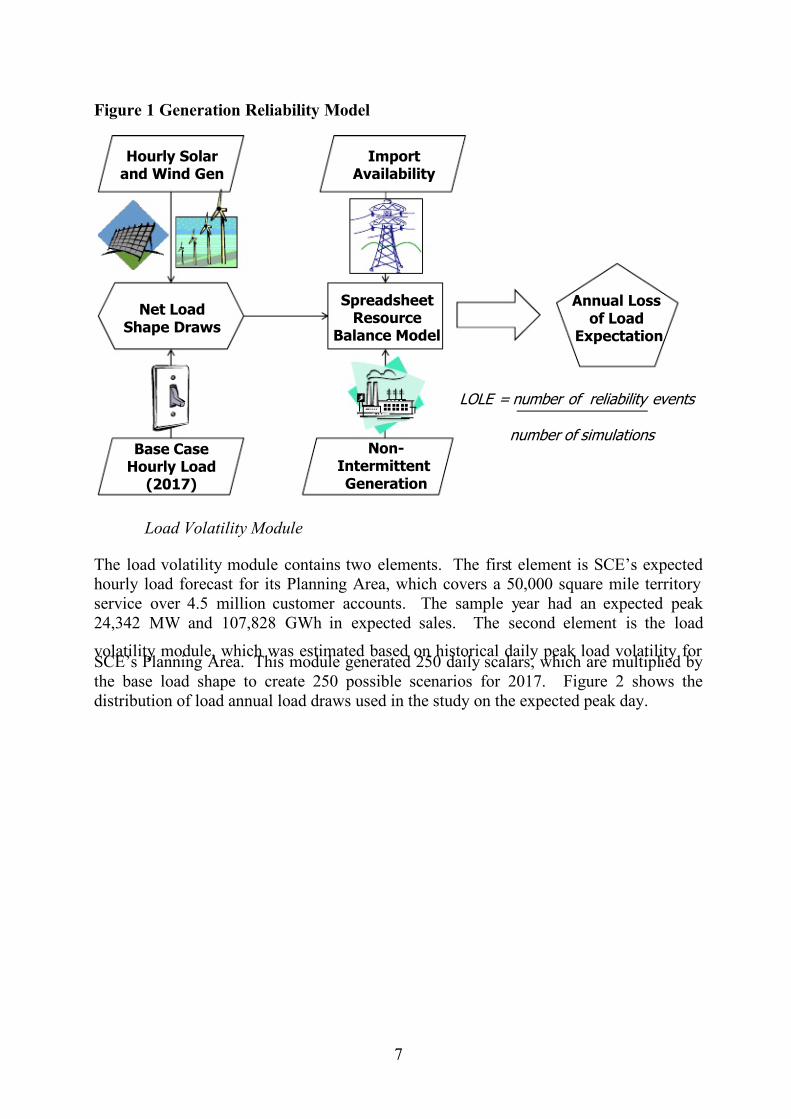
Figure 1 Generation Reliability Model

Load Volatility Module

The load volatility module contains two elements. The first element is SCE’s expectedhourly load forecast for its Planning Area, which covers a 50,000 square mile territory

service over 4.5 million customer accounts. The sample year had an expected peak

24,342 MW and 107,828 GWh in expected sales. The second element is the load

volatility module, which was estimated based on historical daily peak load volatility for SCE’s Planning Area. This module generated 250 daily scalars, which are multiplied by

the base load shape to create 250 possible scenarios for 2017. Figure 2 shows the

distribution of load annual load draws used in the study on the expected peak day.

Annual Lossof Load

Expectation

SpreadsheetResource

Balance Model

LOLE = number of reliability events

number of simulations

Import Availability

Hourly Solarand Wind Gen

Base CaseHourly Load

(2017)

Non-IntermittentGeneration

Net LoadShape Draws



8

Figure 2 Distribution of Load around Expected Annual Peak

Wind and Solar Availability

Hourly wind and solar generation profiles were based on a combination of simulated data

developed as part of the 2010 Long-Term Procurement Plan Proceeding at the California

Public Utilities Commission and historical data from two SCE wind projects. Forecasted

wind and solar generation profiles for the 2017 test year were estimated using the average

of the 2010 LTPP profiles scaled to match SCE’s forecast for total annual gener ationfrom wind, solar photovoltaic, and solar thermal resources delivering to SCE’s Planning

Area. To increase the number of possible generation profiles for any given day in the testyear, the authors randomized daily profiles by month, assuming no correlation with load

or each other. This assumption was made based on a visual inspection of the source 2010

LTPP dataset, which albeit limited, did not show a strong correlation between peak load,solar, and wind output. Figure 3 illustrates the process.

0%

2%

4%

6%

8%

10%

12%

14%

16%

18%

20%

2 1 , 1 7

8

2 1 , 6 1

6

2 2 , 0 5

4

2 2 , 4 9

2

2 2 , 9 3

0

2 3 , 3 6

8

2 3 , 8 0

7

2 4 , 2 4

5

2 4 , 6 8

3

2 5 , 1 2

1

2 5 , 5 5

9

2 5 , 9 9

7

2 6 , 4 3

6

2 6 , 8 7

4

2 7 , 3 1

2

M o r e

F r e q u e n c y

MW

Expected Peak:24,342 MW



9

Figure 3 Approach to Developing Wind and Solar Variability (January)

Non-Intermittent Generation Availability

To model non-intermittent generation, each plant (natural gas, biomass, geothermal,etc...) assumed to be in operation in 2017 was assigned a maximum output rating, annualforced outage rate, and maintenance schedule. The maximum output ratings and annual

forced outage rates were drawn from SCE’s internal database and the Transmission

Expansion Planning Policy Committee (TEPPC) database, which forecasts generationcapacity in the Western Electricity Coordinating Council (WECC) region. Forced outage

scenarios were generated using a random number between 0 and 1. Additionally, the

maximum output ratings were varied by season (winter and summer) to take capturetypical efficiency losses resulting from higher ambient temperatures. The assumed

maintenance schedule was fixed for each load and generation scenario based on the

schedule used in the 2010 Long-Term Procurement Plan Proceeding at the CPUC.

Import Availability

Import availability was modeled in a similar manner as non-intermittent generation.

Eight transmission interties to SCE’s system were modeled assuming fixed summer and

winter import availability with an assumed forced outage rate. To derive availableimports, the authors reviewed total lines flows into SCE’s system from July 2009 to

October 2011. The selection of this data range was based on data availability for the

All Daily SolarProfiles for

January

All Daily WindProfiles for

January

Solar Profile forIteration 1

Wind Profile forIteration 1

Total Solar and WindProfile forIteration 1

Iteration 1

Random selection of 31 Days to Populate

All Daily SolarProfiles for

January

All Daily WindProfiles for

January

Solar Profile forIteration 2

Wind Profile forIteration 2

Total Solar and WindProfile forIteration 2

Iteration 2

Random selection of 31 Days to Populate



10

selected lines. The availability assigned to each line was based on the 99th

percentile of

total imports during the summer on-peak period and the winter mid-peak period for

summer and winter respectively.6

Forced outage rates were also based on historicalrecords from SCE from this same period. Additionally, direct imports were considered.

Outages on a transmission line associated with a direct importing generator limited that

generators availability to serve load in SCE’s territory.

Resource Balance Model

The Resource Balance model combines output from each of the abovementioned modules

and compares system demand and resource available for each hour of the simulation (i.e.

250 hourly load shapes by 750 hourly resource availability shapes). Any day in whichload was greater than the total resource availability in any hour is logged as a loss of load

event. The Resource Balance model calculates the expected number of loss of load

events for the simulation year and records this information at the conclusion of the

simulation.

4. Calculating Effective Load Carrying Capacity

The authors used the resource balance model to calculate the ELCC for a sample of 36wind and solar resources, which were then used to develop the regression approach.

Each of the 36 resources was modeled in a similar manner as the intermittent generation

described above (i.e. daily profiles were randomized by month). The sample resources

were based on a mix of simulated data from the 2010 LTPP and historical SCE data.

ELCC was calculated using the following process. First, a representation of SCE’sPlanning Area was input into the reliability model and baseline reliability level was

calculated. Second, load was added evenly across all hours of the year until the expected

number of loss of load events for the simulation year was one day in ten years. Third, thetest resource profile was added to the model, reducing the expected number of loss of load events to less than one. Finally, load was incrementally added until the expected

number of loss of load events returned to one. The amount of load supported by the test

resource profile was recorded as its ELCC once the simulation was completed. Thefollowing section describes how the results of the reliability model were used to derive

the regression approach.

5. Developing the Regression Approach

In developing the regression approach, the authors assessed three approaches to

estimating ELCC for individual projects: (1) existing CPUC RA accounting rules, (2) an

adjusted percentile approach based on existing CPUC RA accounting rules, and (3) a

6 Summer On-Peak is defined as noon to 6pm on summer weekdays except holidays. Winter Mid-Peak is

defined as 8am to 9pm winter weekdays except holidays. Summer begins June 1st and ends October 1st.



11

regression based approach. The authors used Mean Absolute Percent Error (MAPE)7

to

measure the accuracy of each method. The following section discusses each approach in

turn. The regression based approach has the lowest MAPE and is recommended in thehybrid approach.

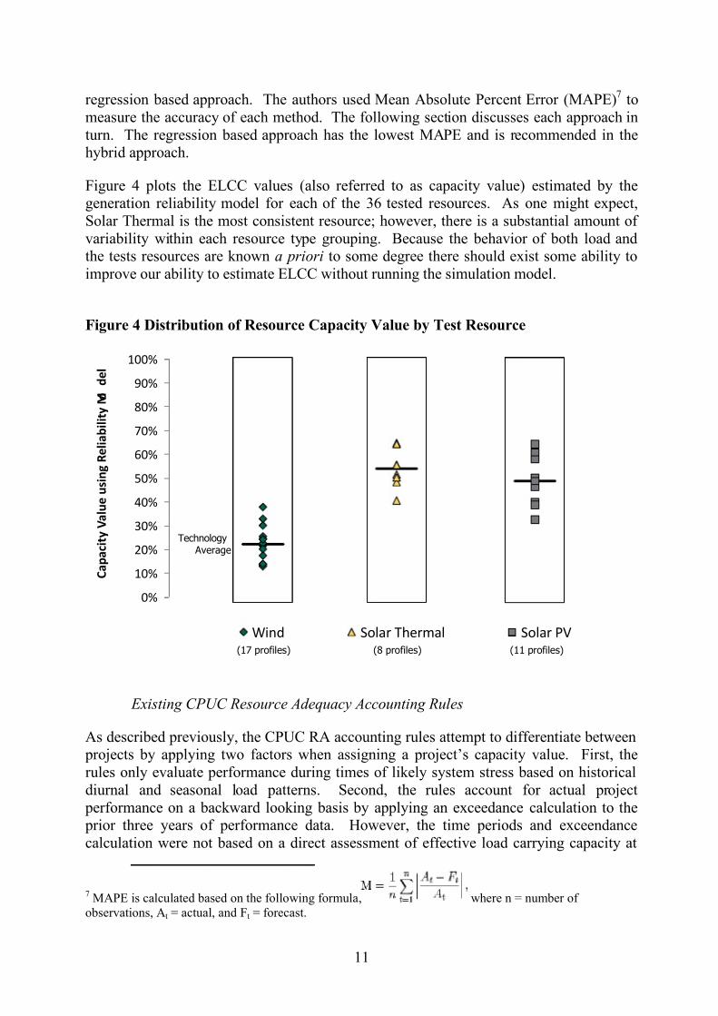
Figure 4 plots the ELCC values (also referred to as capacity value) estimated by thegeneration reliability model for each of the 36 tested resources. As one might expect,

Solar Thermal is the most consistent resource; however, there is a substantial amount of

variability within each resource type grouping. Because the behavior of both load andthe tests resources are known a priori to some degree there should exist some ability to

improve our ability to estimate ELCC without running the simulation model.

Figure 4 Distribution of Resource Capacity Value by Test Resource

Existing CPUC Resource Adequacy Accounting Rules

As described previously, the CPUC RA accounting rules attempt to differentiate between projects by applying two factors when assigning a project’s capacity value. First, the

rules only evaluate performance during times of likely system stress based on historical

diurnal and seasonal load patterns. Second, the rules account for actual project

performance on a backward looking basis by applying an exceedance calculation to the prior three years of performance data. However, the time periods and exceendance

calculation were not based on a direct assessment of effective load carrying capacity at

7 MAPE is calculated based on the following formula, where n = number of

observations, At = actual, and Ft = forecast.

0%

10%

20%

30%

40%

50%

60%

70%

80%

90%

100%

C a p a c i t y V a l u e u s i n g R e l i a b i l i t y M o

d e l

Wind Solar Thermal Solar PV

Technology Average

(17 profiles) (8 profiles) (11 profiles)



12

the time they were developed. Figure 5 plots the relationship between the annual

effective load carrying capacity of the test resources (y-axis) and the average summer

capacity value calculated using the existing RA accounting rules. The solid black linerepresents perfect correlation between reliability model and the RA accounting rules.

Table 1 records the MAPE statistics.

Figure 5 Reliability Model versus Current RA Accounting Rules

Table 1 MAPE Statistics for Current RA Accounting Rules

Category MAPE

Wind 72%Solar Thermal 10%

Solar PV 10%Weighted Average 39%

Based on these results, the reliability model attributes much more value to wind than do

the current RA accounting rules. In contrast, the reliability model and the current RA

accounting rules are well aligned for solar PV and solar thermal. Importantly, the RA

0%

10%

20%

30%

40%

50%

60%

70%

80%

90%

100%

0% 10% 20% 30% 40% 50% 60% 70% 80% 90% 100%

Wind

Solar Thermal

Solar PV

R e l i a b i l i t y M o

d e l

Current RA Accounting Rules (Summer Average)



13

accounting rules are able to place more value on better performing solar projects and less

value on worse performing solar projects, indicating that the framework may be able to

reasonably estimate the reliability model output.

Adjusted Percentile Approach

Applying the same framework as the current RA accounting rules, the authors used an

optimization routine to determine the percentile, months, and hours of the day thatminimized the approach’s overall MAPE. Figure 6 plots the values determined by the

adjusted percentile approach against the effective load carrying capacity values calculated

using the reliability based model. Table 2 shows the resulting MAPE statistics.

Figure 6 Reliability Model versus Adjusted Percentile Approach

Table 2 MAPE Statistics for Adjusted Percentile Approach

Category MAPE

Wind 24.2%

Solar Thermal 6.2%Solar PV 6.6%

Total 15%

0%

10%

20%

30%

40%

50%

60%

70%

80%

90%

100%

0% 10% 20% 30% 40% 50% 60% 70% 80% 90% 100%

Wind

Solar Thermal

Solar PV

R

e l i a b i l i t y M o d e l

Adjusted Percentile Approach



14

The adjusted percentile approach is a marked improvement over the current RA

accounting rules. The MAPE statistics improve for all technology categories and wind is

now reasonably predicted by the calculation. However, the approach suffers in a fewareas. First, the method produced sample criteria and percentiles that differ between

technologies. This result is not immediately intuitive. Second, a few obvious outliers

exist within the wind sample. Some additional metrics may capture other characteristicsof the underlying resource characteristics that could explain these differences.

A Regression-based Approach

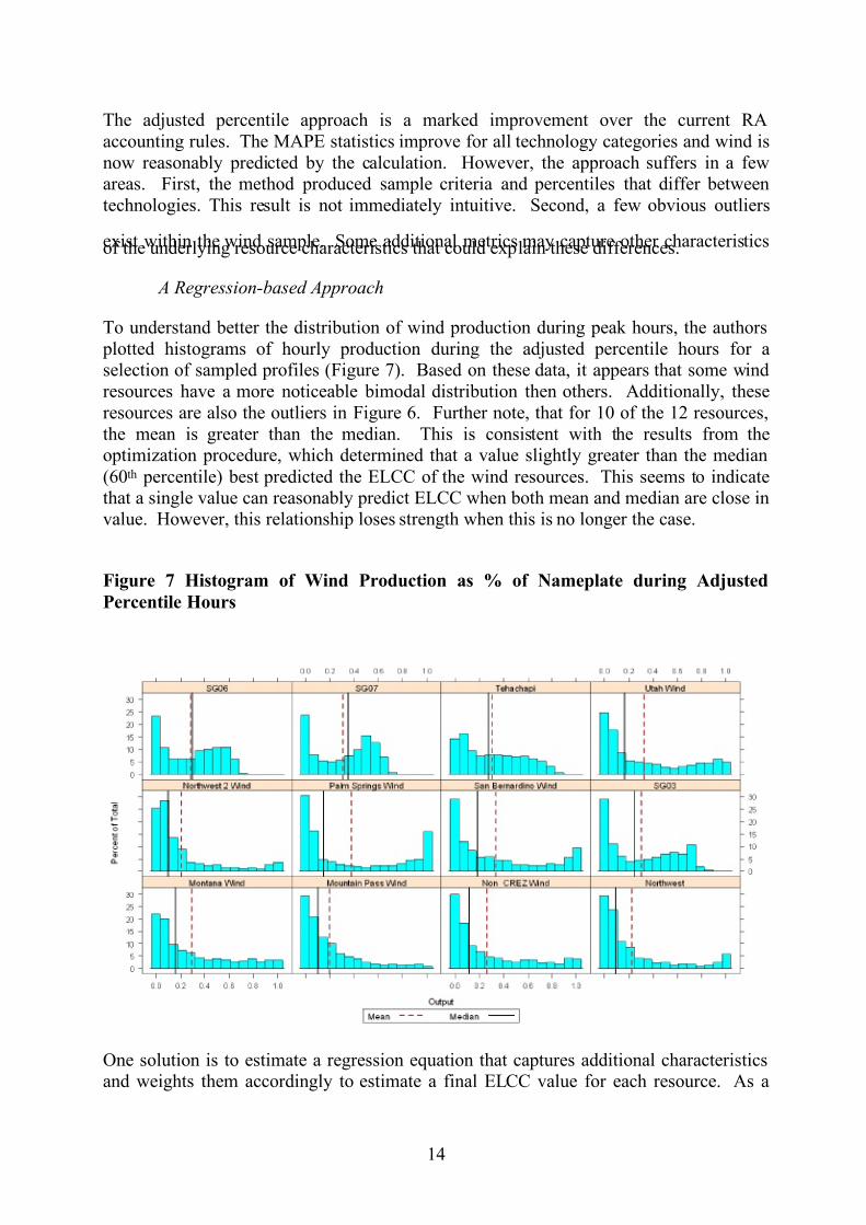
To understand better the distribution of wind production during peak hours, the authors

plotted histograms of hourly production during the adjusted percentile hours for aselection of sampled profiles (Figure 7). Based on these data, it appears that some wind

resources have a more noticeable bimodal distribution then others. Additionally, these

resources are also the outliers in Figure 6. Further note, that for 10 of the 12 resources,

the mean is greater than the median. This is consistent with the results from theoptimization procedure, which determined that a value slightly greater than the median

(60th percentile) best predicted the ELCC of the wind resources. This seems to indicatethat a single value can reasonably predict ELCC when both mean and median are close invalue. However, this relationship loses strength when this is no longer the case.

Figure 7 Histogram of Wind Production as % of Nameplate during Adjusted

Percentile Hours

One solution is to estimate a regression equation that captures additional characteristicsand weights them accordingly to estimate a final ELCC value for each resource. As a



15

robust statistic, the authors continued to rely on percentiles and developed the following

equation.

The 45th percentile is a measure of central tendency during the sample period (i.e. June to

October, hour ending 14 to 20), while the difference between the 90th

and the 45th

percentile captures the relative spread of the data. This variable rewards projects that

may produce at a high level during periods of system stress. The exact variabledefinitions and sample periods were guided by the authors, but selected using

optimization. Finally, the functional form was selected based on visually inspecting the

residuals of a purely linear specification.

Figure 8 shows the capacity value determined by the regression approach against the

effective load carrying capacity values calculated using the reliability based model.Table 4 shows the regression out and MAPE statistics. From Figure 8, we can see that

outliers no longer exist for the wind category. Further, the estimates for solar were alsounaffected, with no noticeable decrease in the predictive power of the estimation modelrelative to the adjusted percentile approach for this category. This analysis indicates that

the results from the reliability simulation model can be estimated by a simple regression

using a priori information about the underlying distribution of wind and solar production.



16

Figure 8 Reliability Model versus Regression Approach

Table 3 Results for Regression Approach

Statistics

Multiple R 97.3%

R Square 94.6%

Adjusted R Square 94.1%Standard Error 4.1%

MAPE – Solar 6.5%

MAPE – Wind 12.5%MAPE – Total 9.3%

Observations 36

Coefficients P-valueIntercept 0.33 0.00004

45t

Percentile 0.58 0.00000

90 Percentile - 45 Percentile (0.94) 0.00004(90

tPercentile - 45

tPercentile)^2 1.00 0.00000

Based on this analysis, the authors propose using a reliability model to estimate ELCCfor a sample of project and then calibrating a regression model as done here. This

R e l i a b i l i t y M o d e l

Regression Approach

0%

10%

20%

30%

40%

50%

60%

70%

80%

90%

100%

0% 10% 20% 30% 40% 50% 60% 70% 80% 90% 100%

Wind

Solar Thermal

Solar PV



17

proposed hybrid approach is a compromise between the ease of the proxy methods and

the accuracy of the reliability method in calculating ELCC, with significant improvement

over the proxy methods. The regression approach also has the advantage of the proxymethods in that individual project perform is reflected in the outcome, and it can be done

on an annual basis. Remaining challenges are the selection of how many technology and

location groups for reliability modeling and how frequently the reliability modeling needsto be performed to reflect resource and load mix changes. The authors suggest a 3-5 year time horizon while monitoring the changing resource mix and load patterns to determine

the need for an update.

6. Conclusion

For planning and procurement purposes, regulators and utility planners need to have an

understanding of the contribution that existing and planning resources make to the

reliability of the generation system. This is especially important as intermittent

resources, such as wind and solar, become major elements of the system’s resource mix. However, existing methods for estimating the contribution of wind and solar to system

reliability present challenges to regulators and utility planners seeking to estimateaccurately the value of many different resources and/or on a frequent basis.

The results of the analysis presented indicate that the proposed hybrid approach has the potential to provide accurate estimates of ELCC for many solar and wind projects,

provided effort is initially expended to develop the regression approach. Further, the

approach is both more accurate and more flexible than the three other methods evaluated.

However, limitations to this study include data available and the evaluation footprint.Lacking significantly diverse performance data for wind and much historical data for

solar PV, the authors relied mostly on simulated profiles. Additionally, the authors

evaluated SCE Planning Area. Implementation at a regional level should consider

transmission limitations between regions and possibly correlations between loads, wind,and solar across these regions.

Using Regression Estimation to Calculate Effective Load Carrying Capacity of Renewable Resources

Documents

Transcript of Using Regression Estimation to Calculate Effective Load Carrying Capacity of Renewable Resources