Using Intraseasonal Indices in Daily Forecast Preparation

Miles Schumacher – NWS Forecast Office Des Moines, IA

Why would you want to look at intraseasonal indices? Intraseasonal indices can suggestinsight into the week 1-3 timescale and reflect local or regional state of the atmosphere. At first it may seem that using intraseasonal atmospheric indices is something that onlyresearchers use. The idea of using intraseasonal indices stems from the concept ofpresented by Len Snellman in the COMET module “Forecast Process”. In a nutshell, theidea of the Forecast Funnel is presented whereby one begins the forecast process bylooking at the large scale, then looking at the smaller scale.

The idea of using intraseasonal indices is analogous to the use of teleconnections of 500mb height patterns in forecasting. “Tele” is from the Greek meaning distance; henceteleconnection simply means distance connection. Simply put, “if this happens here, thatwill happen there” type of thinking. There area several intraseasonal patterns that we canuse as forecasters to help give insights into weather behavior. Often, knowledge of thecause of effect brought on by various intraseasonal patterns will tip the forecaster off tothe potential of an erroneous model run.

It is important to realize that one can not simply look at one of the indices and assumethat everything will follow just what the teleconnections suggest. Unfortunately, natureis not that simple. Many times one or more of the patterns will interact with each other. One may be clearly dominant, but this is not always the case.

It is important to realize that there are interactions between various intraseasonal patternsand therefore you must look at several. The strength of a particular pattern is importantas one may tend to counter another, or enhance the other, depending on which phase eachone is in.

There area several teleconnection patterns that are important to follow when forecastingtrends in U.S. weather. The most important are, NAO, (North Atlantic Oscilation), WP(West Pacific), EP, (East Pacific), NP, (North Pacific), PNA (Pacific North American),and to a lesser degree, SCAND (Scandinavia), EATL/WRUS, (East Atlantic/WestRussian), and Polar-Eurasia patterns. In addition to teleconnection patterns, perhaps themost significant intraseasonal factor is the MJO, (Madden-Julian Oscilation). TheMadden-Julian Oscillation is the development of periodic tropical convection, occurringon the intraseasonal timescale (in this case every 30-60 days), which in turn interactswith the mid-latitude westerlies. It is a naturally occurring component of the coupledocean-atmosphere system.

I want to start out with a brief review of the influence of MJO on weather patterns aroundthe globe. The MetEd site has a good module on the life cycle of the MJO and can be

found at: http://meted.ucar.edu/climate/mjo/index.htm , other information can be found inthe DLCC course and on the Climate Prediction Center website.

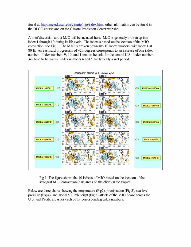
A brief discussion about MJO will be included here. MJO is generally broken up intoindex 1 through 10 during its life cycle. The index is based on the location of the MJOconvection, see Fig 1. The MJO is broken down into 10 index numbers, with index 1 at80 E. An eastward progression of ~20 degrees corresponds to an increase of one indexnumber. Index numbers 9, 10, and 1 tend to be cold for the central U.S. Index numbers3-8 tend to be warm. Index numbers 4 and 5 are typically a wet period.

Fig 1. The figure shows the 10 indices of MJO based on the location of the strongest MJO convection (blue areas on the chart) in the tropics..

Below are three charts showing the temperature (Fig2), precipitation (Fig 3), sea levelpressure (Fig 4), and global 500 mb height (Fig 5) affects of the MJO phase across theU.S. and Pacific areas for each of the corresponding index numbers.

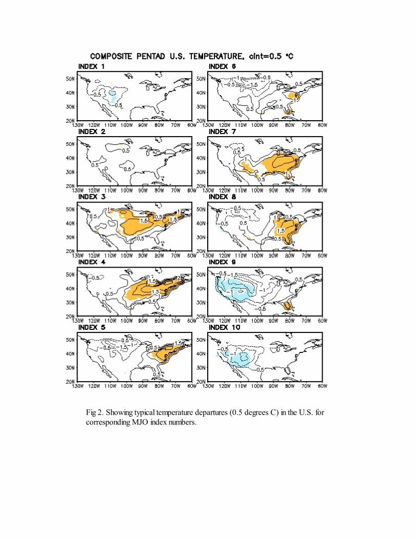
Fig 2. Showing typical temperature departures (0.5 degrees C) in the U.S. forcorresponding MJO index numbers.

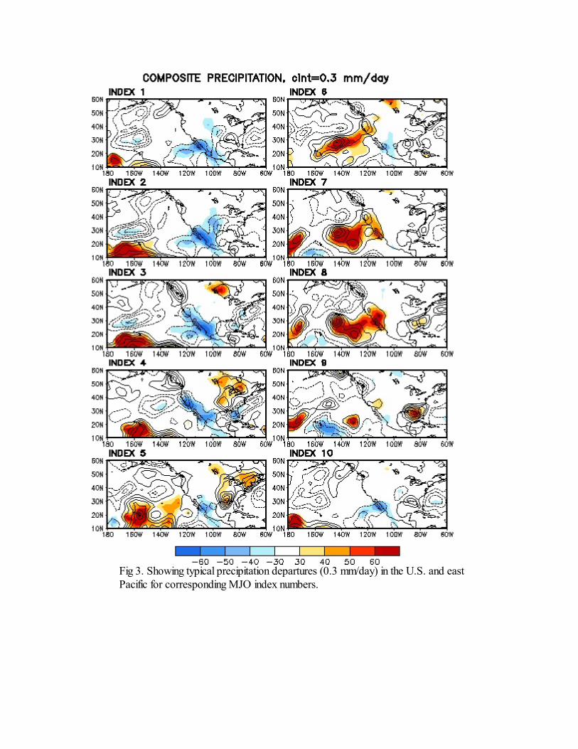
Fig 3. Showing typical precipitation departures (0.3 mm/day) in the U.S. and eastPacific for corresponding MJO index numbers.

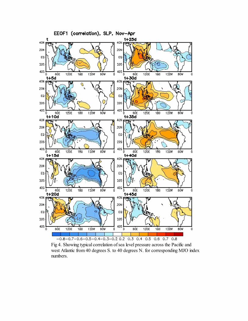
Fig 4. Showing typical correlation of sea level pressure across the Pacific andwest Atlantic from 40 degrees S. to 40 degrees N. for corresponding MJO indexnumbers.

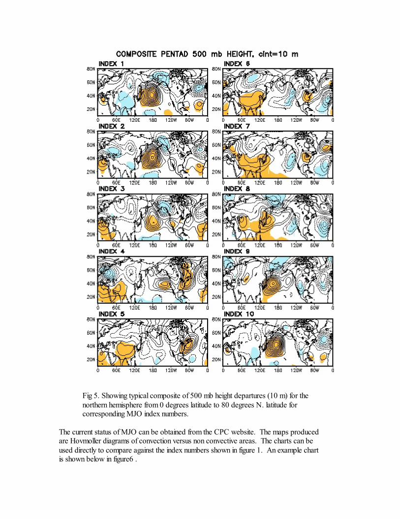
Fig 5. Showing typical composite of 500 mb height departures (10 m) for thenorthern hemisphere from 0 degrees latitude to 80 degrees N. latitude forcorresponding MJO index numbers.

The current status of MJO can be obtained from the CPC website. The maps producedare Hovmoller diagrams of convection versus non convective areas. The charts can beused directly to compare against the index numbers shown in figure 1. An example chartis shown below in figure6 .

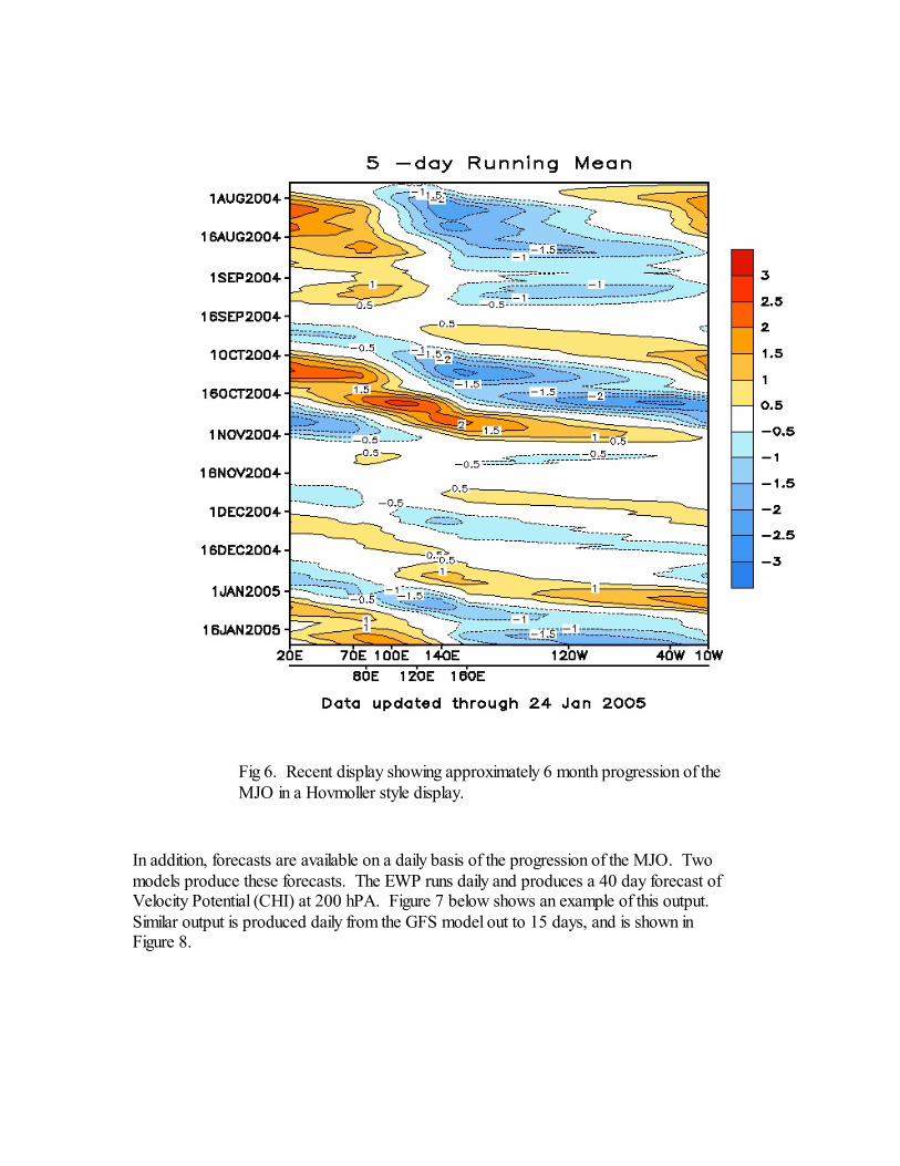
Fig 6. Recent display showing approximately 6 month progression of theMJO in a Hovmoller style display.

In addition, forecasts are available on a daily basis of the progression of the MJO. Twomodels produce these forecasts. The EWP runs daily and produces a 40 day forecast of Velocity Potential (CHI) at 200 hPA. Figure 7 below shows an example of this output. Similar output is produced daily from the GFS model out to 15 days, and is shown inFigure 8.

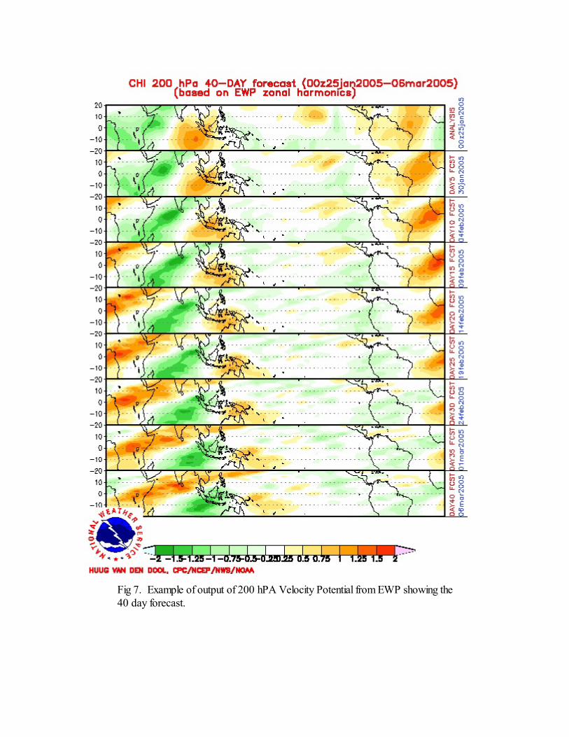
Fig 7. Example of output of 200 hPA Velocity Potential from EWP showing the40 day forecast.

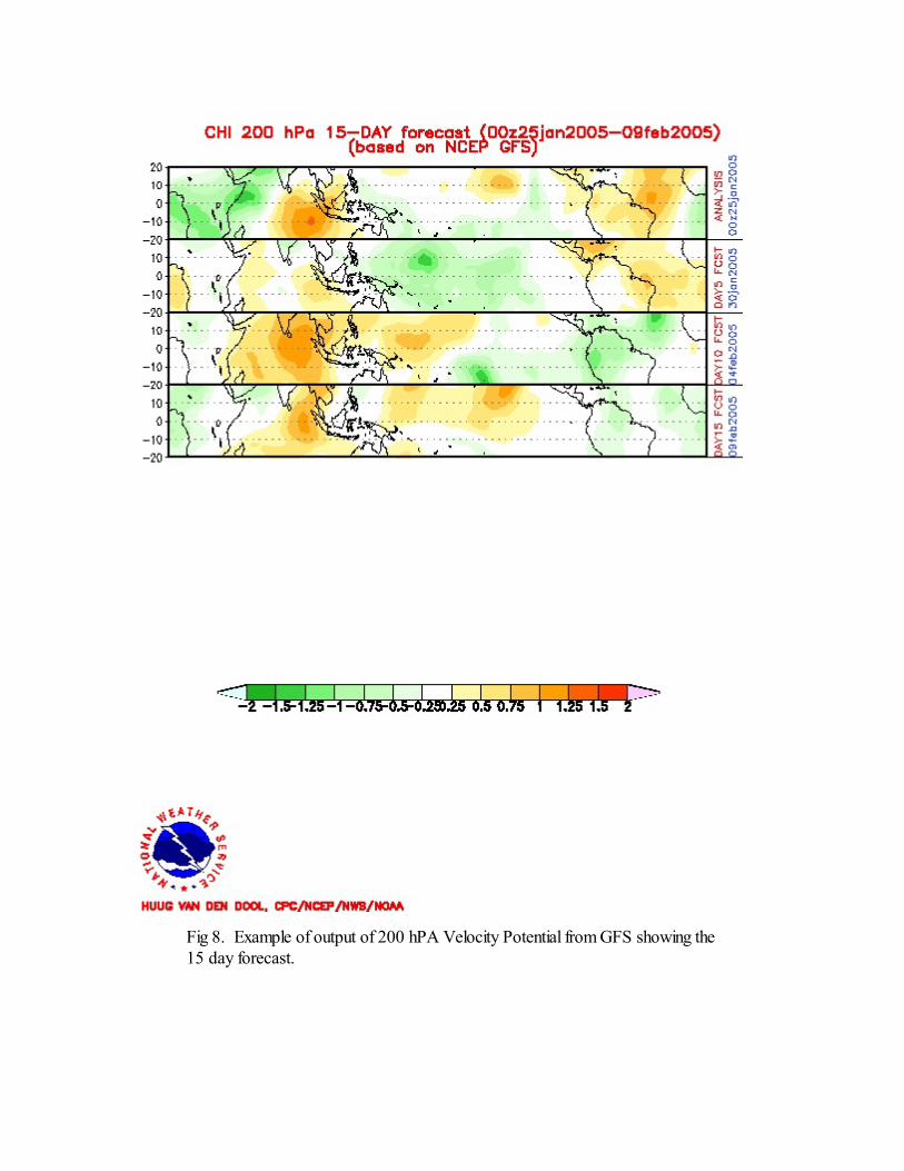
Fig 8. Example of output of 200 hPA Velocity Potential from GFS showing the15 day forecast.

The MJO appears to have the strongest influence on northern hemispheric weatherpatterns, however several other teleconnection patterns need to be considered. Theinformation below was obtained from the CPC website. Forecasts for several of thesepatterns are available from the CPC website out to 15 days as well. Each of the mapsbelow show corresponding 500 mb height departures for the positive phase of theteleconnection for the northern hemisphere. For negative phase, the changes at 500 mbare the opposite.

The MJO had a definite affect on the jet stream pattern. An example of effects on the jetstream is presented below. Though a good example, this sequence of events wassomewhat unusual in that a much stronger than normal Pacific wave train developedduring this period.

The sequence above is a selection of daily mean maps of 250mb vector wind anomalyand are used to summarize the observed circulation anomalies, including the ridges andtroughs that influence local weather. The map here shows the red H's (L's) are theanticyclonic (cyclonic) circulation anomalies, the dashed orange ovals indicate the twin

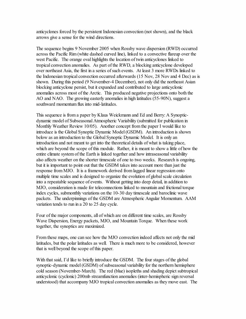
anticyclones forced by the persistent Indonesian convection (not shown), and the blackarrows give a sense for the wind directions.

The sequence begins 9 November 2005 when Rossby wave dispersion (RWD) occurredacross the Pacific Rim (white dashed curved line), linked to a convective flareup over thewest Pacific. The orange oval highlights the location of twin anticyclones linked totropical convection anomalies. As part of the RWD, a blocking anticyclone developedover northeast Asia, the first in a series of such events. At least 3 more RWDs linked tothe Indonesian tropical convection occurred afterwards (15 Nov, 28 Nov and 4 Dec) as isshown. During this period (9 November-4 December), not only did the northeast Asianblocking anticyclone persist, but it expanded and contributed to large anticyclonicanomalies across most of the Arctic. This produced negative projections onto both theAO and NAO. The growing easterly anomalies in high latitudes (55-90N), suggest asouthward momentum flux into mid-latitudes.

This sequence is from a paper by Klaus Weickmann and Ed and Berry: A Synoptic-dynamic model of Subseasonal Atmospheric Variability (submitted for publication inMonthly Weather Review 10/05). Another concept from the paper I would like tointroduce is the Global Synoptic Dynamic Model (GSDM). An introduction is shownbelow as an introduction to the Global Synoptic Dynamic Model. It is only anintroduction and not meant to get into the theoretical details of what is taking place,which are beyond the scope of this module. Rather, it is meant to show a little of how theentire climate system of the Earth is linked together and how intraseasonal variabilityalso affects weather on the shorter timescale of one to two weeks. Research is ongoing,but it is important to point out that the GSDM takes into account more than just theresponse from MJO. It is a framework derived from lagged linear regression ontomultiple time scales and is designed to organize the evolution of global scale circulationinto a repeatable sequence of events. Without getting into deep detail, in addition toMJO, consideration is made for teleconnections linked to mountain and frictional torqueindex cycles, submonthly variations on the 10-30 day timescale and baroclinic wavepackets. The underpinnings of the GSDM are Atmospheric Angular Momentum. AAMvariation tends to run in a 20 to 25 day cycle.

Four of the major components, all of which are on different time scales, are RossbyWave Dispersion, Energy packets, MJO, and Mountain Torque. When these worktogether, the synoptics are maximized.

From these maps, one can see how the MJO convection indeed affects not only the midlatitudes, but the polar latitudes as well. There is much more to be considered, howeverthat is well beyond the scope of this paper.

With that said, I’d like to briefly introduce the GSDM. The four stages of the globalsynoptic-dynamic model (GSDM) of subseasonal variability for the northern hemispherecold season (November-March). The red (blue) isopleths and shading depict subtropicalanticyclonic (cyclonic) 200mb streamfunction anomalies (inter-hemispheric sign reversalunderstood) that accompany MJO tropical convection anomalies as they move east. The

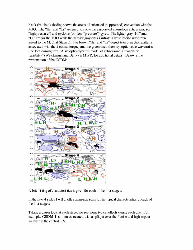
black (hatched) shading shows the areas of enhanced (suppressed) convection with theMJO. The “Hs” and “Ls” are used to show the associated anomalous anticyclonic (or“high pressure”) and cyclonic (or “low “pressure”) gyres. The lighter gray “Hs” and“Ls” are for the MJO while the heavier gray ones illustrate a west Pacific wavetrainlinked to the MJO at Stage 2. The brown “Hs” and “Ls” depict teleconnection patternsassociated with the frictional torque, and the green ones show synoptic-scale wavetrains. See forthcoming text, “A synoptic-dynamic model of subseasonal atmosphericvariability” (Weickmann and Berry) in MWR, for additional details. Below is thepresentation of the GSDM:

A brief listing of characteristics is given for each of the four stages.

In the next 4 slides I will briefly summarize some of the typical characteristics of each ofthe four stages:

Taking a closer look at each stage, we see some typical effects during each one. Forexample, GSDM 1 is often associated with a split jet over the Pacific and high impactweather in the central U.S.

• MJO convection around 110E with enhanced (suppressed) tropical convectiveforcing across the eastern (western) hemisphere;

• Amplified (tropical/subtropical) seasonal base state;• Low AAM / strengthened subtropical momentum sink; • PNA<0 forced by tM-tF index cycle (tM < 0, tF > 0 sequence);• Contracted east Asian and North American jets, displaced poleward/split flows

over the oceans;• The MJO and tM-tF index cycle give large positive frictional torques;• La Nina like base state with Pacific Ocean anticyclonic wave breaking;• Wave energy dispersion favors high impact weather across the USA Plains.

For GSDM 2. Typically one finds a fast moving Pacific wave train. SDM 2 can lead tocold temperatures in the central U.S., especially during the transition from SDM 1 toSDM 2.

• MJO convection around 150E• Eastward shifted seasonal base state;• d(AAM)/dt >0 / momentum sink shifting poleward;• The MJO and fast time scale component give large positive mountain torques;• Western Pacific to North American Rossby wavetrain/strong ridge from USA

west coast into Alaska;• Asian-Pacific wavetrain favors east Pacific cyclonic wave break for transition to

Stage 3;• Much below normal temperatures possible across central and eastern USA.

During GSDM 3 one typically sees high impact weather along the west coast. The jetstream often splits over the continental areas. Temperatures tend to be mild over thecentral and eastern U.S.

• MJO convection around date line with enhanced (suppressed) tropical convectivesignal across the western (eastern) hemisphere;

• Deamplified seasonal base state;• High AAM / weakened subtropical momentum sink; • PNA>0 forced by mountain torque > 0, friction torque < 0 sequence;• Extended east Asian and North American jets, displaced equatorward /split flows

cross the continents;• The MJO and tM-tF index cycle give large negative frictional torques;• El Nino like base state with east Pacific Ocean cyclonic wave breaking;• High impact weather event possible along USA west coast.

During GSDM 4 the westerlies tend to weaken. Temperatures tend to be mild over thecentral and eastern U.S.

• MJO convective signal across the western hemisphere, locations at ~160W, 60Wand 60E

• Westward shifted seasonal base state;• d(AAM)/dt <0 / weakened momentum sink shifting poleward;• MJO and fast component give large negative mountain torque;

• Strong subtropical jets, with subtropical westerlies weakening;• Asian-Pacific wavetrain favors anticyclonic wave break across east Pacific Ocean

for transition to Stage 1;• Heavy precipitation event possible across southwestern USA.

Next I would like to show how we can use the daily MJO charts. In the graphic below, pictured is the 200 mb CHI. Across the top is the MJO index number. Across theBottom are the SDM phase that corresponds to the MJO index number. The vertical linerepresents the core of the MJO convection.

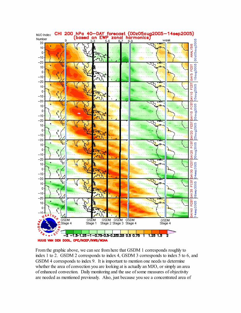
From the graphic above, we can see from here that GSDM 1 corresponds roughly toindex 1 to 2. GSDM 2 corresponds to index 4, GSDM 3 corresponds to index 5 to 6, andGSDM 4 corresponds to index 9. It is important to mention one needs to determinewhether the area of convection you are looking at is actually an MJO, or simply an areaof enhanced convection. Daily monitoring and the use of some measures of objectivityare needed as mentioned previously. Also, just because you see a concentrated area of

convection at index number “x” doesn’t automatically mean that you can assume GSDM“y”. One would need to look further into it, but it would give you some starting point. You may also notice how the convection tends to become weaker or more broken up as itprogresses east. SST’s need to be on the order of 29 C. to support deep tropicalconvection. SST’s tend to be higher in the eastern Hemisphere and is the reason for theapparent weakening of convection.

Moving on to teleconnections patterns I will start below with a chart, table 1, showing thetimes of the year that each pattern has the most significant affect on North America. Thechart shows the ranked importance of each teleconnection pattern. For the purposes ofthis paper, I chose to use only the top three in rank. From the table it is clear to see thatthe strongest influence on North American weather on an annual basis is the NAOpattern. Other patterns are important during various times of the year. The PNA patternis very significant during the cool season for example, while the East Pacific and NorthPacific patterns are most important during the warm season.

Table 1

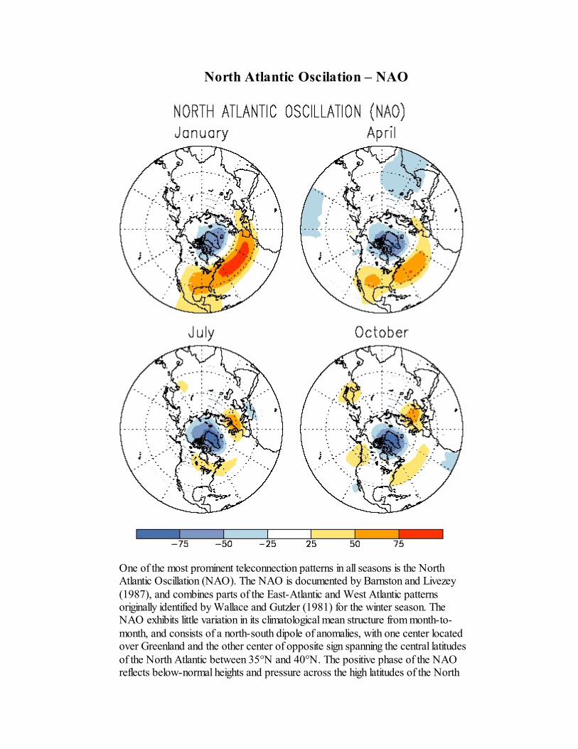
North Atlantic Oscilation – NAO

One of the most prominent teleconnection patterns in all seasons is the NorthAtlantic Oscillation (NAO). The NAO is documented by Barnston and Livezey(1987), and combines parts of the East-Atlantic and West Atlantic patternsoriginally identified by Wallace and Gutzler (1981) for the winter season. TheNAO exhibits little variation in its climatological mean structure from month-to-month, and consists of a north-south dipole of anomalies, with one center locatedover Greenland and the other center of opposite sign spanning the central latitudesof the North Atlantic between 35°N and 40°N. The positive phase of the NAOreflects below-normal heights and pressure across the high latitudes of the North

Atlantic and above-normal heights and pressure over the central North Atlantic,the eastern United States and western Europe. The negative phase reflects anopposite pattern of height and pressure anomalies over these regions. Both phasesof the NAO are associated with basin-wide changes in the intensity and locationof the North Atlantic jet stream and storm track, and in large-scale modulations ofthe normal patterns of zonal and meridional heat and moisture transport (Hurrell1995), which in turn results in changes in temperature and precipitation patternsoften extending from eastern North America to western and central Europe(Walker and Bliss 1932, van Loon and Rogers 1978, Rogers and van Loon 1979).

Strong positive phases of the NAO tend to be associated with above-normaltemperatures in the eastern United States and across northern Europe and below-normal temperatures in Greenland and oftentimes across southern Europe and theMiddle East. They are also associated with above-normal precipitation overnorthern Europe and Scandinavia and below-normal precipitation over southernand central Europe. Opposite patterns of temperature and precipitation anomaliesare typically observed during strong negative phases of the NAO. Duringparticularly prolonged periods dominated by one particular phase of the NAO,abnormal height and temperature patterns are also often seen extending well intocentral Russia and north-central Siberia.

The NAO exhibits considerable interseasonal and interannual variability, andprolonged periods (several months) of both positive and negative phases of thepattern are common. Additionally, the wintertime NAO exhibits significantinterannual and interdecadal variability (Hurrell 1995). For example, the negativephase of the NAO dominated the circulation from the mid-1950's through the1978/79 winter. During this approximately 24-year interval, there were fourprominent periods of at least three years each in which the negative phase wasdominant and the positive phase was notably absent. In fact, during the entireperiod the positive phase was observed in the seasonal mean only three times, andit never appeared in two consecutive years.

An abrupt transition to recurring positive phases of the NAO then occurred duringthe 1979/80 winter, with the atmosphere remaining locked into this mode throughthe 1994/95 winter season. During this 15-year interval, a substantial negativephase of the pattern appeared only twice, in the winters of 1984/85 and 1985/ 86.However, November 1995 - February 1996 (NDJF 95/96) was characterized by areturn to the strong negative phase of the NAO. Halpert and Bell (1997; theirsection 3.3) recently documented the conditions accompanying this transition tothe negative phase of the NAO. The 1996/97 winter season has exhibited a morevariable nature to the NAO, with negative phases of the pattern occurring inDecember 1996 and January 1997, and positive phases occurring in February andMarch 1997.

A representation of typical weather patterns associated the positive and negative phase ofNAO. In the positive phase of NAO, cold air remains to the north of the CONUS in

Canada. During the negative phase of NAO, cold air sinks south into the northeast onethird to one half of the CONUS. (see graphic below).

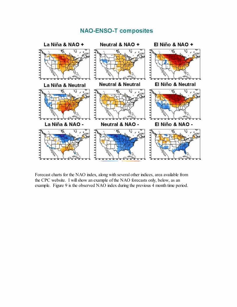
A set of correlation maps is presented here to show the effects of ENSO and NAOcombined. Labels on the chart should be self explanatory.

Forecast charts for the NAO index, along with several other indices, area available fromthe CPC website. I will show an example of the NAO forecasts only, below, as anexample. Figure 9 is the observed NAO index during the previous 4 month time period.

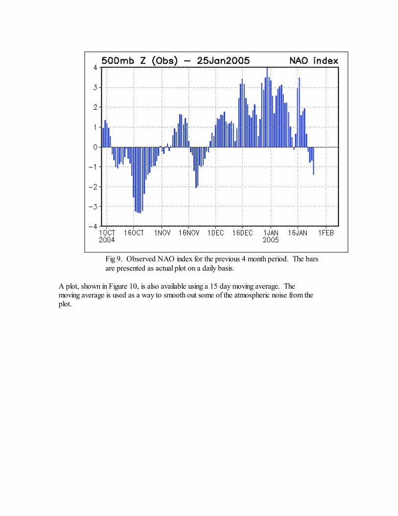
Fig 9. Observed NAO index for the previous 4 month period. The barsare presented as actual plot on a daily basis.

A plot, shown in Figure 10, is also available using a 15 day moving average. Themoving average is used as a way to smooth out some of the atmospheric noise from theplot.

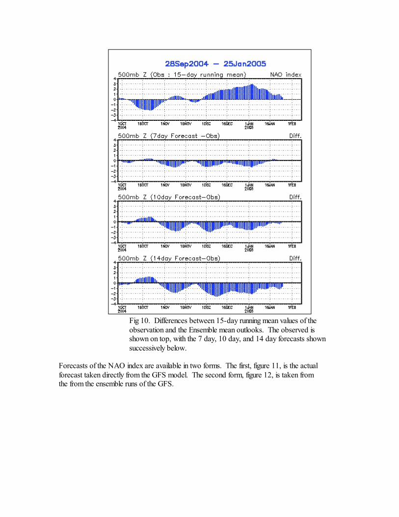
Fig 10. Differences between 15-day running mean values of theobservation and the Ensemble mean outlooks. The observed isshown on top, with the 7 day, 10 day, and 14 day forecasts shownsuccessively below.

Forecasts of the NAO index are available in two forms. The first, figure 11, is the actualforecast taken directly from the GFS model. The second form, figure 12, is taken fromthe from the ensemble runs of the GFS.

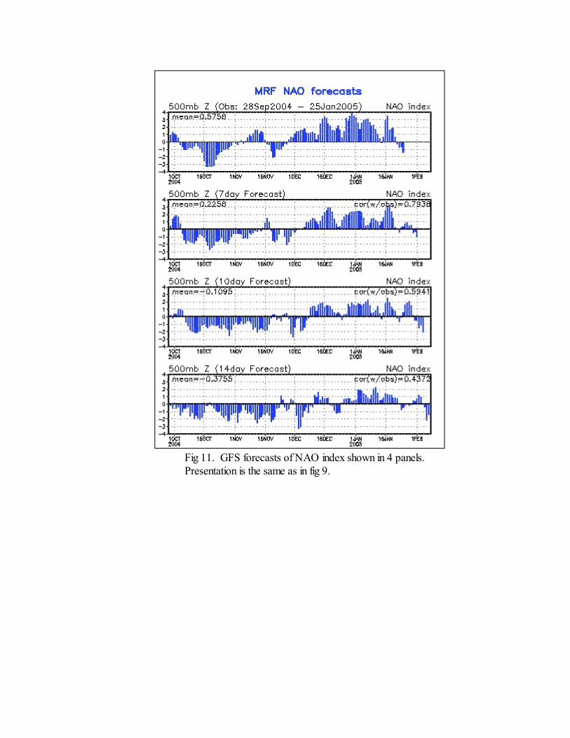
Fig 11. GFS forecasts of NAO index shown in 4 panels. Presentation is the same as in fig 9.

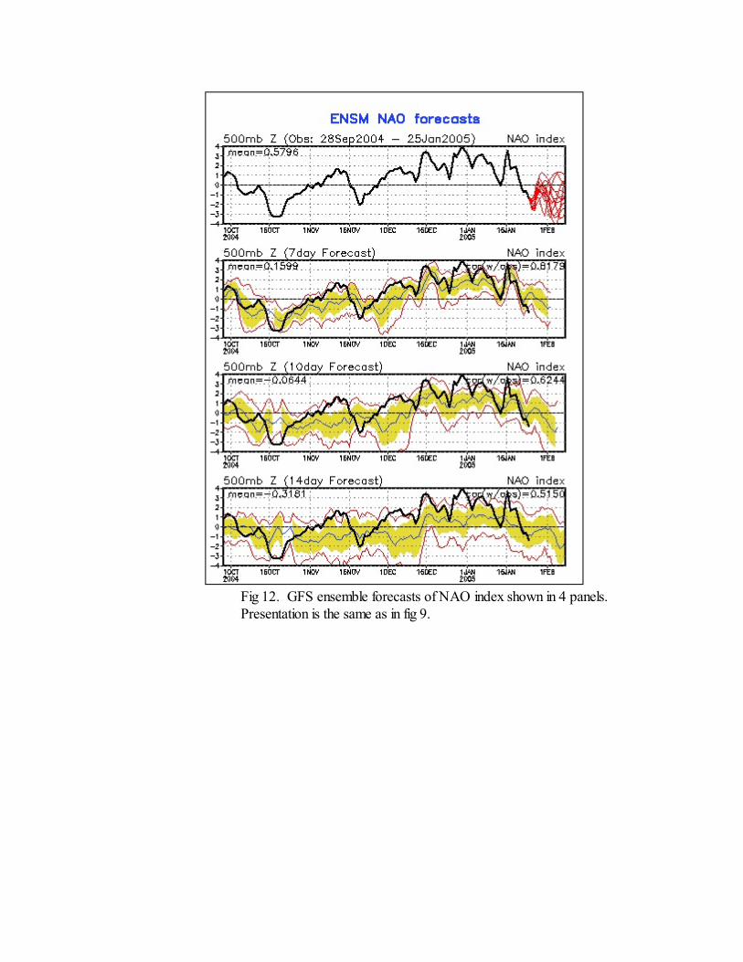
Fig 12. GFS ensemble forecasts of NAO index shown in 4 panels. Presentation is the same as in fig 9.

Pacific North America (PNA)

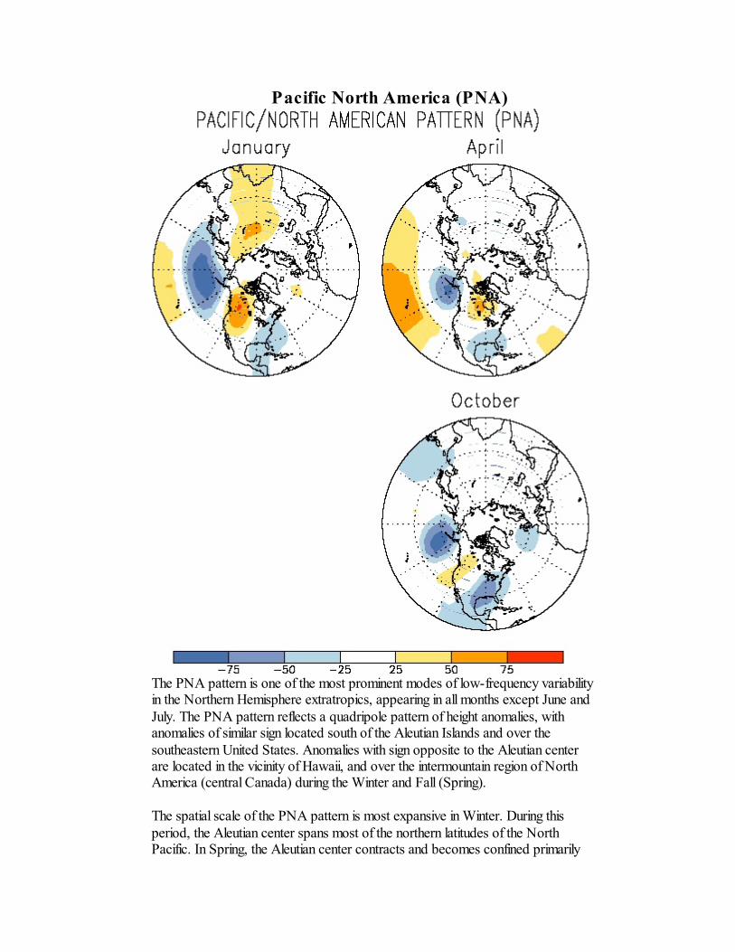
The PNA pattern is one of the most prominent modes of low-frequency variabilityin the Northern Hemisphere extratropics, appearing in all months except June andJuly. The PNA pattern reflects a quadripole pattern of height anomalies, withanomalies of similar sign located south of the Aleutian Islands and over thesoutheastern United States. Anomalies with sign opposite to the Aleutian centerare located in the vicinity of Hawaii, and over the intermountain region of NorthAmerica (central Canada) during the Winter and Fall (Spring).

The spatial scale of the PNA pattern is most expansive in Winter. During thisperiod, the Aleutian center spans most of the northern latitudes of the NorthPacific. In Spring, the Aleutian center contracts and becomes confined primarily

to the Gulf of Alaska. However, the subtropical center near Hawaii reachesmaximum amplitude during the spring. The PNA pattern then disappears duringJune and July, but reappears in the late summer and fall. During this period, themidlatitude centers become dominant and appear as a wave pattern emanatingfrom the eastern North Pacific. The subtropical center near Hawaii is weakestduring this period.

The time series of the PNA pattern also indicates substantial interseasonal,interannual and interdecadal variability. For example, a negative phase of thepattern dominated the period from 1964-1967, while a positive phase of thepattern tended to dominate from 1976-1988. A negative phase of the PNA thendominated during the 1989-1990 period, followed by a prolonged positive phasefrom fall 1991- early spring 1993.

North Pacific Pattern

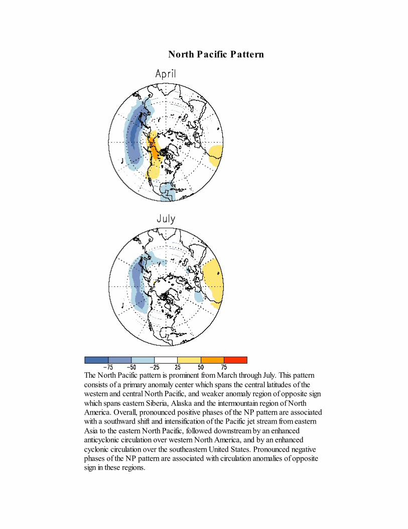
The North Pacific pattern is prominent from March through July. This patternconsists of a primary anomaly center which spans the central latitudes of thewestern and central North Pacific, and weaker anomaly region of opposite signwhich spans eastern Siberia, Alaska and the intermountain region of NorthAmerica. Overall, pronounced positive phases of the NP pattern are associatedwith a southward shift and intensification of the Pacific jet stream from easternAsia to the eastern North Pacific, followed downstream by an enhancedanticyclonic circulation over western North America, and by an enhancedcyclonic circulation over the southeastern United States. Pronounced negativephases of the NP pattern are associated with circulation anomalies of oppositesign in these regions.

Bell and Janowiak (1995) recently noted that a positive phase of the NP patternreflects one of the preferred responses of the extratropical atmospheric circulationto ENSO during the Northern Hemisphere spring. This response was particularlyevident during the 1992 and 1993 spring seasons, when a prolonged positivephase of the NP pattern dominated the circulation.

Bell and Janowiak also note that the atmospheric circulation during the severalmonth period prior to the onset of the Midwest floods of June-July 1993 wasdominated by the most pronounced and persistent positive phase of the NP patternin the historical record. Their study concluded that these conditions wereindirectly important to the onset and overall magnitude of the floods, since theyfostered an anomalously intense storm track over the midlatitudes of the NorthPacific. Dramatic changes in this storm track during June then ultimately initiatedthe Midwest floods.

East Pacific Pattern

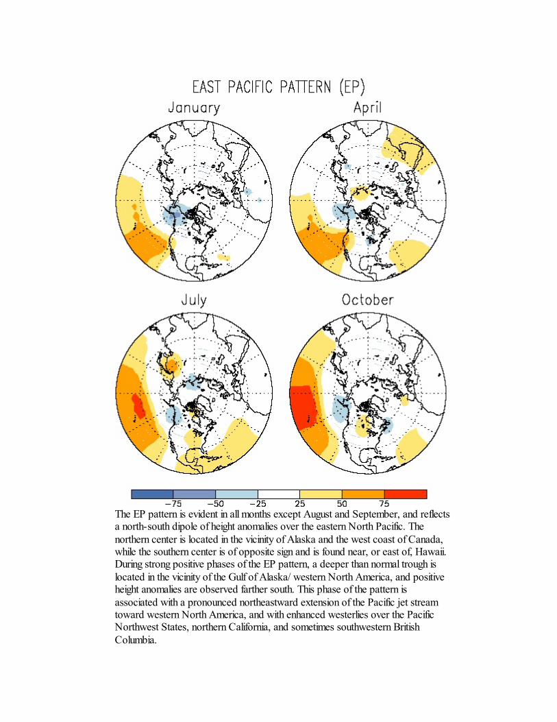
The EP pattern is evident in all months except August and September, and reflectsa north-south dipole of height anomalies over the eastern North Pacific. Thenorthern center is located in the vicinity of Alaska and the west coast of Canada,while the southern center is of opposite sign and is found near, or east of, Hawaii.During strong positive phases of the EP pattern, a deeper than normal trough islocated in the vicinity of the Gulf of Alaska/ western North America, and positiveheight anomalies are observed farther south. This phase of the pattern isassociated with a pronounced northeastward extension of the Pacific jet streamtoward western North America, and with enhanced westerlies over the PacificNorthwest States, northern California, and sometimes southwestern BritishColumbia.

In contrast, strong negative phases of the EP pattern are associated with apronounced split-flow configuration over the eastern North Pacific, and withreduced westerlies throughout the region. This circulation is accompanied by aconfinement of the climatological mean Pacific trough to the western NorthPacific, and possibly with a blocking flow configuration farther east.

The most persistent positive phase of the EP-Jet pattern occurred from 1973-1975, and the most persistent negative phase of the pattern occurred from early1992 through mid-1993. This latter period was dominated by warm episodeconditions in the equatorial Pacific, and by two distinct periods of mature ENSOconditions. During this period, the subtropical jet stream was generally strongerthan normal and displaced well east of its climatological -mean position towardthe southwestern United States. These conditions contributed to an end ofprolonged drought conditions in California (Bell and Basist 1994), and broughtabundant precipitation to the southwestern United States, particularly during the1992/93 winter. These conditions were also associated with generally above-normal precipitation over the central United States during the year preceding theonset of the Midwest floods of June-July 1993 (Bell and Janowiak 1995, Chagnon1996). This enhanced precipitation then contributed to above-normal soilmoisture levels throughout the Midwest during the period, and to near-saturatedsoil conditions just prior to the onset of the floods.

East Atlantic Jet Pattern

The East Atlantic Jet pattern is the third primary mode of low frequencyvariability found over the North Atlantic, appearing between April and August.This pattern also consists of a north-south dipole of anomaly centers, with onemain center located over the high latitudes of the eastern North Atlantic andScandinavia, and the other center located over Northern Africa and theMediterranean Sea. A positive phase of the EA-Jet pattern reflects anintensification of westerlies over the central latitudes of the eastern North Atlanticand over much of Europe, while a negative phase reflects a strong split-flowconfiguration over these regions, sometimes in association with long-livedblocking anticyclones in the vicinity of Greenland and Great Britain

The time series of the EA-jet pattern exhibits considerable interdecadalvariability. For example, the 1971-1978 period is dominated by the negativephase of the pattern, while the 1985-1993 period is dominated by the positivephase of the pattern. In fact, from 1986-1993 the positive phase of the pattern wasobserved nearly 70% of the time.

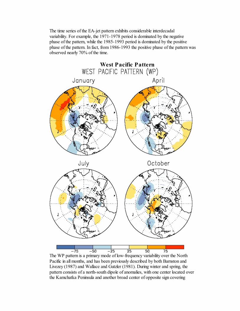
West Pacific Pattern

The WP pattern is a primary mode of low-frequency variability over the NorthPacific in all months, and has been previously described by both Barnston andLivezey (1987) and Wallace and Gutzler (1981). During winter and spring, thepattern consists of a north-south dipole of anomalies, with one center located overthe Kamchatka Peninsula and another broad center of opposite sign covering

portions of southeastern Asia and the low latitudes of the extreme western NorthPacific. Therefore, strong positive or negative phases of this pattern reflectpronounced zonal and meridional variations in the location and intensity of theentrance region of the Pacific (or East Asian) jet steam.

In the summer and fall, the WP pattern becomes increasingly wave-like, and athird prominent center appears over Alaska and the Beaufort Sea, with a signopposite to the center over the western North Pacific. This wave structure is mostevident in the Fall, when it extends downstream along a quasi great-circle routeinto the western United States. The time series of the WP pattern indicatesconsiderable intermonthly and interannual variability, and persistence of aparticular phase of the pattern is relatively common.

East Atlantic/West Russia Pattern

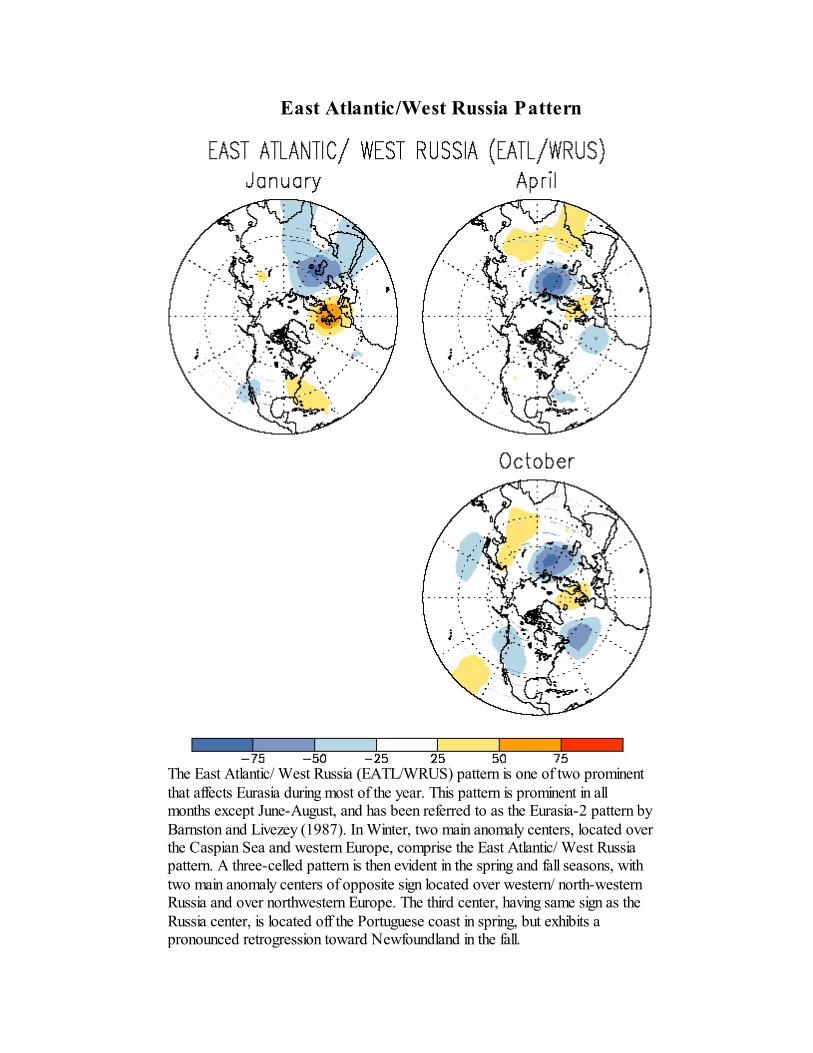
The East Atlantic/ West Russia (EATL/WRUS) pattern is one of two prominentthat affects Eurasia during most of the year. This pattern is prominent in allmonths except June-August, and has been referred to as the Eurasia-2 pattern byBarnston and Livezey (1987). In Winter, two main anomaly centers, located overthe Caspian Sea and western Europe, comprise the East Atlantic/ West Russiapattern. A three-celled pattern is then evident in the spring and fall seasons, withtwo main anomaly centers of opposite sign located over western/ north-westernRussia and over northwestern Europe. The third center, having same sign as theRussia center, is located off the Portuguese coast in spring, but exhibits apronounced retrogression toward Newfoundland in the fall.

The most pronounced and persistent negative phases of the East Atlantic/ WestRussia pattern tend to occur in winter and early spring, with particularly largenegative phases noted during the winters and early springs of 1969/70, 1976/77and 1978/79. Pronounced positive phases of the pattern are less common, with themost prominent positive phase evident during late winter/ early spring of1992/93. During this 1992/93 winter, negative height anomalies were observedthroughout western and southwestern Russia, and positive height anomalies wereobserved throughout Europe and the eastern North Atlantic. These conditionswere accompanied by warmer and wetter than normal conditions over largeportions of Scandinavia and northwestern Russia, and by much colder and drierthan normal conditions over the eastern Mediterranean Sea and the Middle East.During MAM 1993, the area of negative anomalies over western Russia persisted,the positive anomaly center over northwestern Europe became consolidated, and anegative anomaly center became established over the eastern North Atlantic.These conditions brought a continuation of warmer (colder) than normalconditions to Scandinavia (eastern Mediterranean Sea sector), and drier thannormal conditions to much of Europe.

Scandinavia Pattern

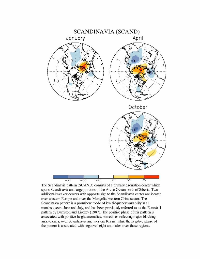
The Scandinavia pattern (SCAND) consists of a primary circulation center whichspans Scandinavia and large portions of the Arctic Ocean north of Siberia. Twoadditional weaker centers with opposite sign to the Scandinavia center are locatedover western Europe and over the Mongolia/ western China sector. TheScandinavia pattern is a prominent mode of low frequency variability in allmonths except June and July, and has been previously referred to as the Eurasia-1pattern by Barnston and Livezey (1987). The positive phase of this pattern isassociated with positive height anomalies, sometimes reflecting major blockinganticyclones, over Scandinavia and western Russia, while the negative phase ofthe pattern is associated with negative height anomalies over these regions.

The time series for the Scandinavia pattern also exhibits relatively largeinterseasonal, interannual and interdecadal variability. For example, a negativephase of the pattern dominated the circulation from early 1964 through mid-1968and from mid-1986 through early 1993. Negative phases of the pattern have alsobeen prominent during winter 1988/89, spring 1990, and winter/spring 1991/92.In contrast, positive phases of the pattern were observed during much of 1972,1976 and 1984.

Polar/Eurasian Pattern

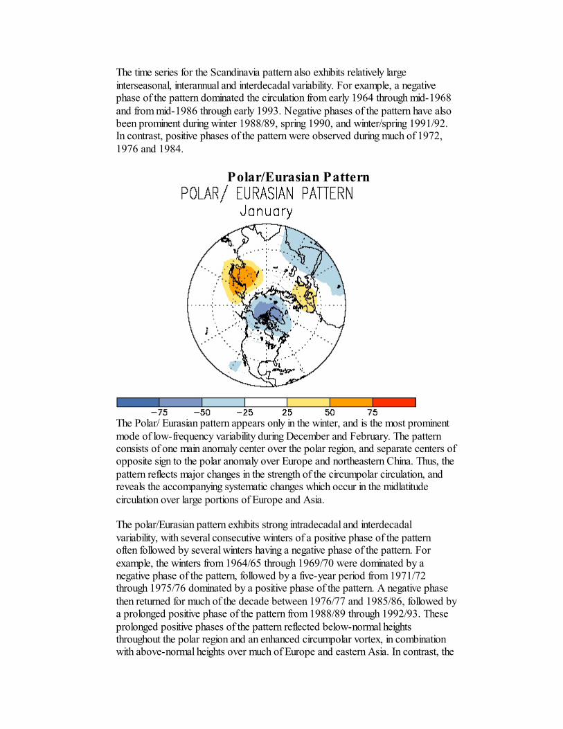
The Polar/ Eurasian pattern appears only in the winter, and is the most prominentmode of low-frequency variability during December and February. The patternconsists of one main anomaly center over the polar region, and separate centers ofopposite sign to the polar anomaly over Europe and northeastern China. Thus, thepattern reflects major changes in the strength of the circumpolar circulation, andreveals the accompanying systematic changes which occur in the midlatitudecirculation over large portions of Europe and Asia.

The polar/Eurasian pattern exhibits strong intradecadal and interdecadalvariability, with several consecutive winters of a positive phase of the patternoften followed by several winters having a negative phase of the pattern. Forexample, the winters from 1964/65 through 1969/70 were dominated by anegative phase of the pattern, followed by a five-year period from 1971/72through 1975/76 dominated by a positive phase of the pattern. A negative phasethen returned for much of the decade between 1976/77 and 1985/86, followed bya prolonged positive phase of the pattern from 1988/89 through 1992/93. Theseprolonged positive phases of the pattern reflected below-normal heightsthroughout the polar region and an enhanced circumpolar vortex, in combinationwith above-normal heights over much of Europe and eastern Asia. In contrast, the

prolonged negative phases of the pattern reflected above-normal heightsthroughout the polar region and a weaker than normal polar vortex, incombination with below-normal heights over much of Europe and eastern Asia.

The following two patterns do not has as strong of a correlation with theweather patterns as the previous patterns, however at the times they area important they may have strong affects on the western U.S. and Alaska.

Pacific Transition Pattern

The Pacific Transition pattern is prominent between May-August. The modeconsists of a wave-like pattern of height anomalies, which extends from the Gulfof Alaska eastward to the Labrador Sea, and is aligned along the 40oN latitudecircle. The prominent centers of action have a similar sign, and are located overthe intermountain region of the United States and over the Labrador Sea.Relatively weak anomaly centers with signs opposite to the above are locatedover the Gulf of Alaska and over the eastern United States.

Two of the most pronounced negative phases of the PT pattern in the historicalrecord occurred during July 1992 and July 1993. During each of these periods,well below-normal 500-mb heights were observed over the northwestern UnitedStates, in association with a substantially reduced strength of the climatologicalmean ridge, which is located over this region in Summer. Below-normal heightswere also observed over the Canadian Maritime Provinces and over the centralNorth Pacific during these months, while above-normal heights were observedover the Gulf of Alaska. During July 1993, these extremely anomalous conditionswere associated with a continuation of record flooding throughout the MidwestUnited States (Bell and Janowiak 1995).

Tropical/Northern Hemisphere Pattern

The Tropical/ Northern Hemisphere pattern was first classified by Mo andLivezey (1986), and appears as a prominent mode from November-February. Thepattern consists of one primary anomaly center over the Gulf of Alaska and aseparate anomaly center of opposite sign over the Hudson Bay. A weaker area ofanomalies having similar sign to the Gulf of Alaska anomaly extends acrossMexico and the extreme southeastern United States. This pattern reflects large-scale changes in both the location and eastward extent of the Pacific jet stream,and also in the strength and position of the climatological mean Hudson Bay Low.Thus, the pattern significantly modulates the flow of marine air into NorthAmerica, as well as the southward transport of cold Canadian air into the north-central United States.

Pronounced negative phases of the TNH pattern are often observed duringDecember and January when Pacific warm (ENSO) episode conditions arepresent (Barnston et al. 1991). One recent example of this is the 1994/95 winterseason, when mature Pacific warm episode conditions and a strong negative phaseof the TNH pattern were present. During this period, the mean Hudson Baytrough was much weaker than normal and shifted northeastward toward theLabrador Sea. Additionally, the Pacific jet stream was much stronger than normaland shifted southward to central California, well south of its climatological meanposition in the Pacific Northwest. This flow pattern brought well above-normaltemperatures to eastern North America and above-normal rainfall to thesouthwestern United States.

In contrast, positive phases of the TNH pattern tend to accompany Pacific coldevents. An example is the very persistent positive phase of the TNH pattern

during 1988/89 -1990/91, which developed in apparent association with thestrong 1988/89 Pacific cold event.

Will using the MJO and various teleconnections guarantee you a perfect forecast? Theanswer is, certainly not. The advantage of using these tools is that you will be able tomake more sound decisions and judgments as you look at the numerical model output,especially in the medium and longer range. This will become more important as we moveinto more active involvement with the forecast in the 8 to 14 day timeframe.

I’d like to go over a few cases briefly to show the potential of using the informationpresented here. I chose several cases to go through fairly briefly to demonstrate not onlyhow the information can be useful, but to show there is a linkage between theintraseasonal indices and the forecast process. Also, note I was able to find not just one,but 5 cases over a period of just two months.

From the 200 hPa Velocity Potential chart shown on the left, we can see that for 10March it would appear we were around index 7 as far as MJO, or at least MJO likeconvection, was concerned. If that was the only thing you looked at, you would expectthe weather to be warm. Indeed, this was not the case. How can that happen?

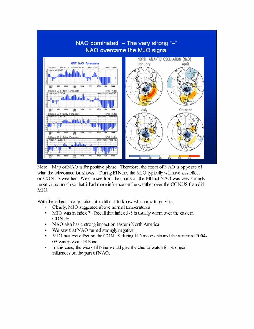
Note – Map of NAO is for positive phase. Therefore, the effect of NAO is opposite ofwhat the teleconnection shows. During El Nino, the MJO typically will have less effecton CONUS weather. We can see from the charts on the left that NAO was very stronglynegative, so much so that it had more influence on the weather over the CONUS than didMJO.

With the indices in opposition, it is difficult to know which one to go with. • Clearly, MJO suggested above normal temperatures• MJO was in index 7. Recall that index 3-8 is usually warm over the eastern

CONUS• NAO also has a strong impact on eastern North America• We saw that NAO turned strongly negative• MJO has less effect on the CONUS during El Nino events and the winter of 2004-

05 was in weak El Nino.• In this case, the weak El Nino would give the clue to watch for stronger

influences on the part of NAO.

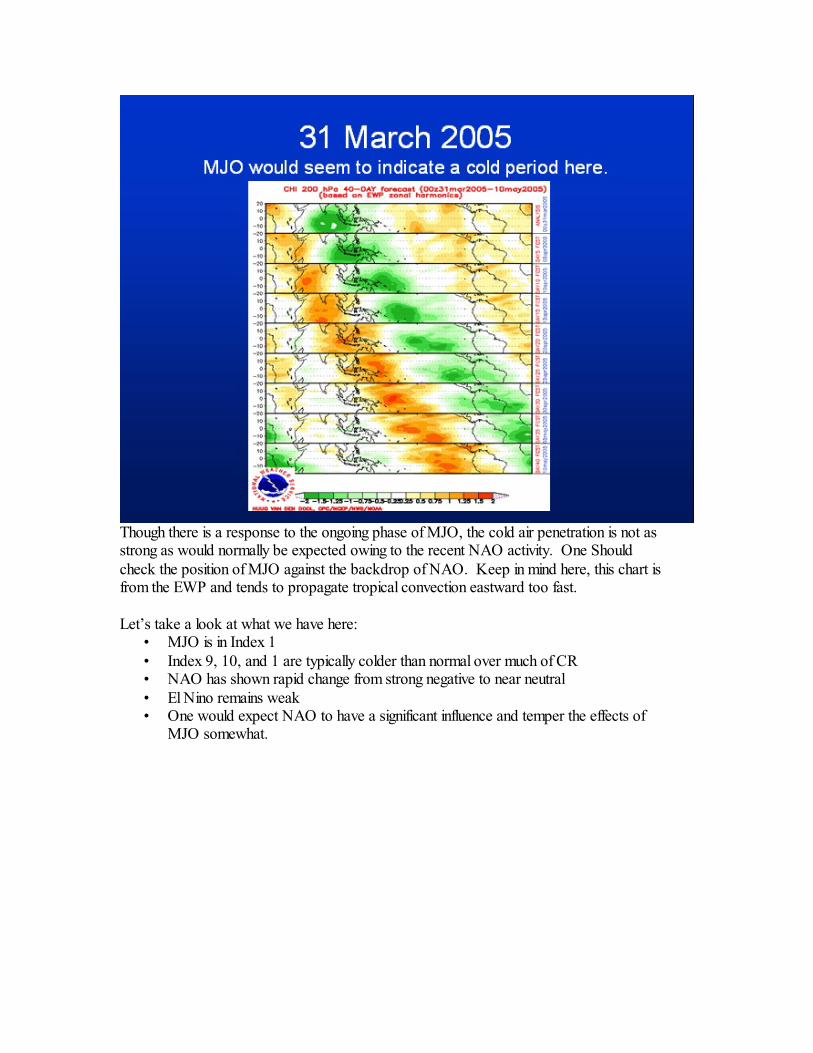
Though there is a response to the ongoing phase of MJO, the cold air penetration is not asstrong as would normally be expected owing to the recent NAO activity. One Shouldcheck the position of MJO against the backdrop of NAO. Keep in mind here, this chart isfrom the EWP and tends to propagate tropical convection eastward too fast.

Let’s take a look at what we have here:• MJO is in Index 1• Index 9, 10, and 1 are typically colder than normal over much of CR• NAO has shown rapid change from strong negative to near neutral• El Nino remains weak• One would expect NAO to have a significant influence and temper the effects of

MJO somewhat.

Note: It was a cool pattern but not extreme.

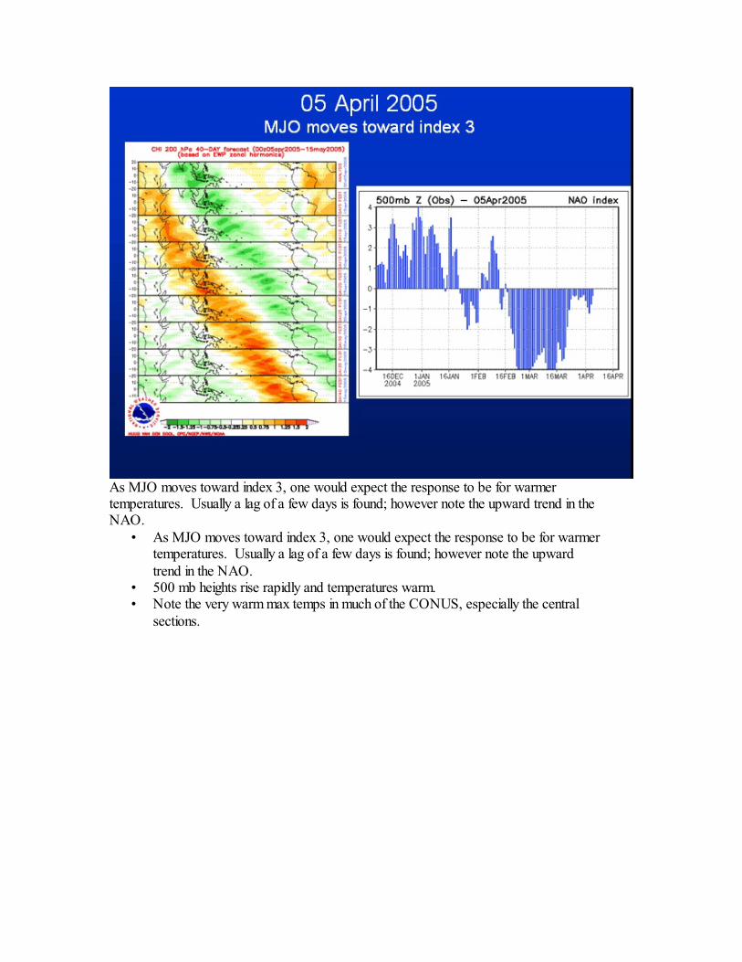
As MJO moves toward index 3, one would expect the response to be for warmertemperatures. Usually a lag of a few days is found; however note the upward trend in theNAO.

• As MJO moves toward index 3, one would expect the response to be for warmertemperatures. Usually a lag of a few days is found; however note the upwardtrend in the NAO.

• 500 mb heights rise rapidly and temperatures warm.• Note the very warm max temps in much of the CONUS, especially the central

sections.

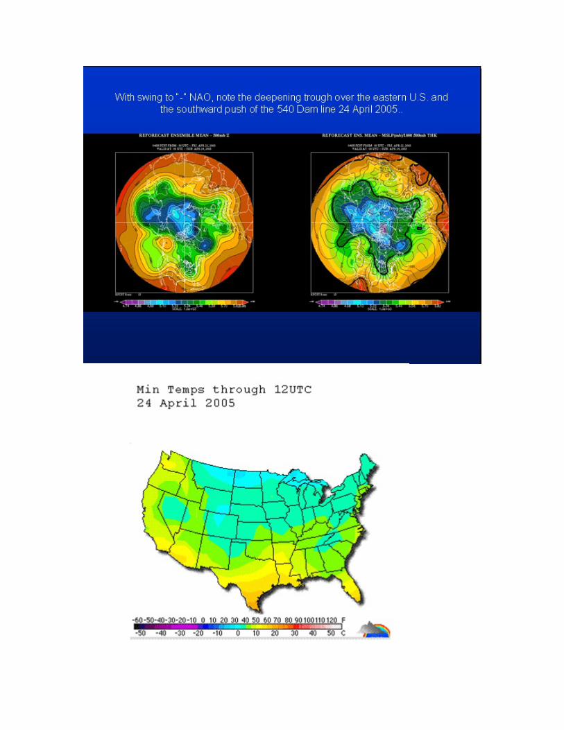
Shown above are the reforecast ensemble MSLP with 1000-500 thickness on the left, andensemble mean 500 mb height on the right for 12 UTC 05 April 2005. Below are maxtemperatures for the day. These readings are very much above normal over the centralU.S. for example. Note the highs in the 70s and 80s as far north as southeast ND intocentral MN.

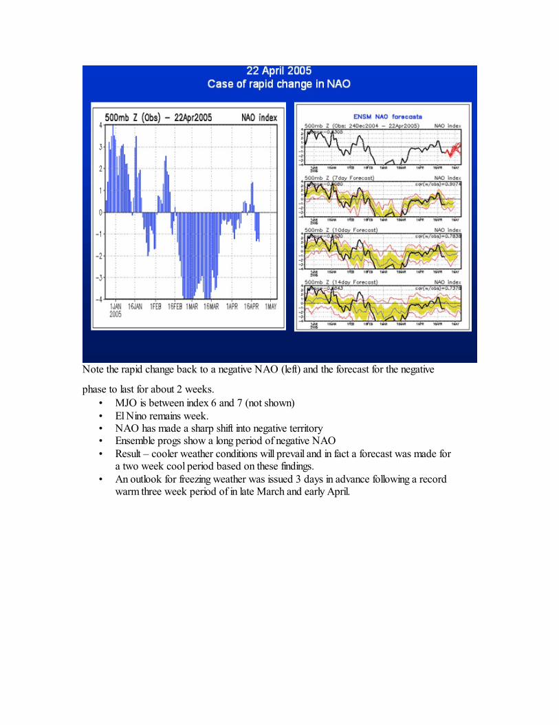
Note the rapid change back to a negative NAO (left) and the forecast for the negative

phase to last for about 2 weeks. • MJO is between index 6 and 7 (not shown)• El Nino remains week.• NAO has made a sharp shift into negative territory• Ensemble progs show a long period of negative NAO• Result – cooler weather conditions will prevail and in fact a forecast was made for

a two week cool period based on these findings. • An outlook for freezing weather was issued 3 days in advance following a record

warm three week period of in late March and early April.

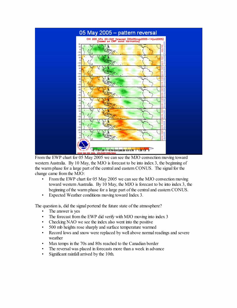
From the EWP chart for 05 May 2005 we can see the MJO convection moving towardwestern Australia. By 10 May, the MJO is forecast to be into index 3, the beginning ofthe warm phase for a large part of the central and eastern CONUS. The signal for thechange came from the MJO:

• From the EWP chart for 05 May 2005 we can see the MJO convection movingtoward western Australia. By 10 May, the MJO is forecast to be into index 3, thebeginning of the warm phase for a large part of the central and eastern CONUS.

• Expected Weather conditions moving toward Index 3.

The question is, did the signal portend the future state of the atmosphere?• The answer is yes• The forecast from the EWP did verify with MJO moving into index 3• Checking NAO we see the index also went into the positive• 500 mb heights rose sharply and surface temperature warmed• Record lows and snow were replaced by well above normal readings and severe

weather• Max temps in the 70s and 80s reached to the Canadian border• The reversal was placed in forecasts more than a week in advance• Significant rainfall arrived by the 10th.

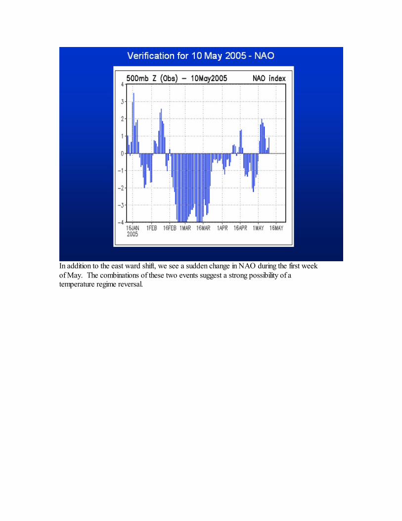
In addition to the east ward shift, we see a sudden change in NAO during the first weekof May. The combinations of these two events suggest a strong possibility of atemperature regime reversal.

After a record cold snap in late April and early May, the pattern underwent a suddenreversal as NAO flipped from negative to positive and MJO began to move into the index3 position. This can be seen in the maximum temperature graphic below:

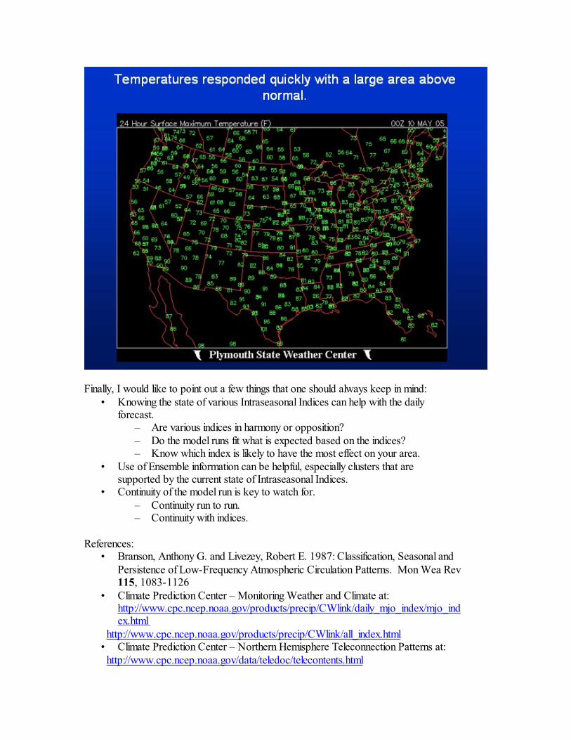
Finally, I would like to point out a few things that one should always keep in mind:• Knowing the state of various Intraseasonal Indices can help with the daily

forecast.– Are various indices in harmony or opposition?– Do the model runs fit what is expected based on the indices?– Know which index is likely to have the most effect on your area.

• Use of Ensemble information can be helpful, especially clusters that aresupported by the current state of Intraseasonal Indices.

• Continuity of the model run is key to watch for.– Continuity run to run.– Continuity with indices.

References:• Branson, Anthony G. and Livezey, Robert E. 1987: Classification, Seasonal and

Persistence of Low-Frequency Atmospheric Circulation Patterns. Mon Wea Rev115, 1083-1126

• Climate Prediction Center – Monitoring Weather and Climate at: http://www.cpc.ncep.noaa.gov/products/precip/CWlink/daily_mjo_index/mjo_index.html

http://www.cpc.ncep.noaa.gov/products/precip/CWlink/all_index.html • Climate Prediction Center – Northern Hemisphere Teleconnection Patterns at:

http://www.cpc.ncep.noaa.gov/data/teledoc/telecontents.html

• Madden, Roland, NCAR (Retired) Foresight Weather: NCAR COMET Programat: http://meted.ucar.edu/climate/mjo/index.htm

• Non-Operational Web Side of HUUG VAN DEN DOOL at the ClimatePrediction Center, Center, National Centers for Environmental Prediction at:

http://www.cpc.ncep.noaa.gov/products/people/wd51hd/ • Weickmann, Klaus and Berry, Edward 2005: A Synoptic-dynamic model of

Subseasonal Atmospheric Variability (submitted for publication in MonthlyWeather Review 10/05) orhttp://www.cdc.noaa.gov/MJO/Predictions/wb2006.pdf

• http://www.cdc.noaa.gov/people/klaus.weickmann/disc092804/Weather_Climate_Discussion_28SEP04.html

Additional Links:SSEC-http://www.ssec.wisc.edu/data/geo/mtsat/ http://www.ssec.wisc.edu/data/geo/met5/

MJO Information-http://www.cpc.ncep.noaa.gov/products/precip/CWlink/daily_mjo_index/mjo_index.shtml http://www.cpc.ncep.noaa.gov/products/precip/CWlink/MJO/mjo.shtmlhttp://www.cpc.ncep.noaa.gov/products/precip/CWlink/ http://www.cdc.noaa.gov/people/klaus.weickmann/disc021506/weather_climate_discussion_10Feb06.html

Teleconnection – Atmospheric monitoring indices-http://www.cpc.ncep.noaa.gov/products/precip/CWlink/all_index.htmlhttp://www.cpc.ncep.noaa.gov/data/teledoc/telecontents.shtml

Helpful MJO and Atmospheric State discussions- Atmospheric Insights - http://weatherclimatelink.blogspot.comExpert MJO Discussionshttp://www.cdc.noaa.gov/MJO/Forecasts/climate_discussions.html (intermittent)