Using Deep Learning to Estimate Tropical Cyclone Intensity fromSatellite Passive Microwave Imagery

ANTHONY WIMMERS AND CHRISTOPHER VELDEN

Cooperative Institute for Meteorological Satellite Studies, University of Wisconsin–Madison, Madison, Wisconsin

JOSHUA H. COSSUTH

Remote Sensing Division, U.S. Naval Research Laboratory, Washington, D.C.

(Manuscript received 8 November 2018, in final form 22 March 2019)

ABSTRACT

A deep learning convolutional neural network model is used to explore the possibilities of estimating

tropical cyclone (TC) intensity from satellite images in the 37- and 85–92-GHz bands. The model, called

‘‘DeepMicroNet,’’ has unique properties such as a probabilistic output, the ability to operate from partial

scans, and resiliency to imprecise TC center fixes. The 85–92-GHz band is the more influential data source

in the model, with 37GHz adding a marginal benefit. Training the model on global best track intensities

produces model estimates precise enough to replicate known best track intensity biases when compared to

aircraft reconnaissance observations. Model root-mean-square error (RMSE) is 14.3 kt (1 kt ’ 0.5144m s21)

compared to two years of independent best track records, but this improves to an RMSE of 10.6 kt when

compared to the higher-standard aircraft reconnaissance-aided best track dataset, and to 9.6 kt compared to the

reconnaissance-aided best track when using the higher-resolution TRMMTMI andAquaAMSR-Emicrowave

observations only. A shortage of training and independent testing data for category 5 TCs leaves the results at

this intensity range inconclusive. Based on this initial study, the application of deep learning to TC intensity

analysis holds tremendous promise for further development with more advanced methodologies and ex-

panded training datasets.

1. Introduction

Deep learning (DL) is a newly popular, powerful and

often confounding computational tool for developing

predictive models in the sciences. It builds on a long

legacy of neural network modeling, with a key feature

being the organization of neural connections into multi-

ple layers of nonlinear operations, enabling models

to apply high levels of abstraction in their tasks.

New hardware innovations, particularly in accessing

graphical processing units (GPUs), have enabled DL

algorithms to become powerful enough to rival hu-

man performance at complicated tasks such as image

classification (He et al. 2016). However, unlike most

other computational methods that are applied to

scientific problems, DL models can paradoxically

achieve high predictive performance (Schmidhuber

2015; LeCun et al. 2015) but a DL model’s methods

are difficult to practically untangle from its network

architecture in a way that derives meaningful scientific

information.

While the broader field of machine learning has had

a long and fruitful application to meteorology (see Haupt

et al. 2008; McGovern et al. 2017 and references therein),

the state of the science of DL applied to meteorology

is limited but rapidly growing. A large portion of work

in this field to date applies to short-term forecasting

for renewable energy (Diaz et al. 2015; Wan et al. 2016;

Sogabe et al. 2016; Hu et al. 2016). Other major research

includes feature identification for long-term climate

analysis (Kurth et al. 2018) and augmenting the output of

precipitation models with two-level DL techniques (Tao

et al. 2016, 2018; Tao and Gao 2017). Recently, Pradhan

et al. (2018) andChen et al. (2018) introducedDLmodels

applied to infrared and morphed rain rate images of

Corresponding author:AnthonyWimmers,wimmers@ssec.wisc.edu

Publisher’s Note: This article was revised on 9 July 2019 to cor-

rect a typographical error in Table 3 that was present when origi-

nally published.

JUNE 2019 W IMMERS ET AL . 2261

DOI: 10.1175/MWR-D-18-0391.1

� 2019 American Meteorological Society. For information regarding reuse of this content and general copyright information, consult the AMS CopyrightPolicy (www.ametsoc.org/PUBSReuseLicenses).

Unauthenticated | Downloaded 10/17/21 12:01 AM UTC

hurricanes, and these are discussed in detail later. The

proliferation of recent conference abstracts on DL in

meteorology also shows the impressive growth of this

field in the past year (e.g., Prabhat et al. 2019; Lagerquist

et al. 2019; Stewart et al. 2019; Gagne et al. 2019;Wu et al.

2019; Boukabara et al. 2019; Hall et al. 2019).

Tropical cyclone (TC) nowcasting is particularly well

suited for DL applications. Operational TC intensity

analysis remains largely dependent on quasi-subjective

techniques such as the Dvorak technique (Dvorak 1984;

Velden et al. 2006), requires intensive analyst training,

and lacks a formal incorporation of imagery beyond vis-

ible and infrared window frequencies. Furthermore, a

new generation of infrared imagers (Schmit et al. 2005,

2017) and emerging cubesat sensors (Blackwell et al.

2012; Cahoy et al. 2015; Reising et al. 2016) require

new, robust techniques for TC nowcasting and forecasting

that can assimilate a spectrally diverse variety of im-

ages all at once.

It is well known that the microwave imaging frequen-

cies available on polar-orbiting meteorological satellites

since the late 1980s offer unique perspectives for ob-

serving TCs. Uses of the imagery for TC applications

have been well documented in earlier studies (e.g.,

Velden et al. 1989; Cecil and Zipser 1999; Hawkins

et al. 2001; Kieper and Jiang 2012; Jiang 2012; Edson

2014). The majority of these were based on qualitative

image assessment or empirical analysis. More analyt-

ical approaches to examining microwave imagery have

revealed ways to nowcast/forecast intensity variations

from eyewall replacement cycles (Sitkowski et al.

2011) and rapid intensification (Rozoff et al. 2015). In

these efforts, the 85–92-GHz band in the horizontal po-

larization (hereafter ‘‘89-GHz band’’) is the most in-

fluential microwave band because of its superior

representation of TC structures revealed by ice

scattering in heavily convective areas. Early attempts

by Bankert and Tag (2002) to use the information

content of this band to estimate the full range of TC

intensities proved to be less effective than IR-based

methods such as the Dvorak technique. Neverthe-

less, there are several unique advantages of the 89-GHz

band for estimating TC intensity, such as depicting

eyewall/banding structure during central dense over-

cast environments. (There are also weaknesses, such

as poor resolution of very small TCs or the lack of

motion-resolving detail.) Bankert and Cossuth (2016)

have begun to capitalize on these advantages with a

decision tree algorithm that separates 89-GHz images

of TCs into different regimes such as shallow systems,

asymmetric systems and eye scenes. Jiang et al. (2019)

demonstrate a skillful regression model to estimate

TC intensity using large-scale TRMM 89-GHz spatial

features. A DL model could incorporate these same re-

lationships implicitly as well. Furthermore, the 89-GHz

band is well suited for exploration with DL because

nearly all the important structural information can be

captured in relatively low-resolution (5km) grids, facili-

tating fast computation. The 37-GHz band, on the other

hand, has a coarser resolution depending on the sensor,

but can be interpolated to 5-km grids with no loss in in-

formation. Other frequency bands have even lower res-

olution on the SSM/I and SSMIS sensors, and therefore

do not correspond closely enough to be used as an ade-

quate counterpart to the 37- and 89-GHz bands.

Non-DL methods using satellite sources besides the

37- and 89-GHz bands have set the current standard for

accurate, automated estimation of TC intensity. These

include using AMSU microwave soundings to measure

the TC warm core anomaly (Brueske and Velden 2003;

Demuth et al. 2004, 2006; Herndon and Velden 2014),

quantifying the finescale radial TC structure in geosta-

tionary infrared (Geo IR) imagery (Piñeros et al. 2008;Ritchie et al. 2012, 2014), and automating and enhancing

the logic of the Dvorak technique with Geo IR (Olander

and Velden 2007, 2018). The root-mean-square error

(RMSE) of these methods ranges from 10 to 15kt (1kt’0.5144ms21). Each has advantages and limitations dis-

cussed in section 6, so further improvements in satellite-

based objective intensity estimates are desirable.

This paper introduces a DL model designed to esti-

mate TC intensity using 37- and 89-GHz band imagery.

In doing so, we explore the potential of this application

of DL to 1) classify satellite microwave images to com-

pete in performance with existing subjective and auto-

mated analysis methods, 2) provide reliable uncertainty

information to accompany its output, and 3) improve the

understanding of certain TC-related aspects of 37- and

89-GHz sensor capabilities in areas that have not been

well addressed. Even though the technique requires an

introduction to many new concepts in machine learning,

the particular DL model applied here is a simple one. As

such, this study focuses on the kind ofmodel performance

that is easily achievable and able to be improved with

further development. Thus we present theDLmodel that

follows as a demonstration of capabilities and not a final

operational version.

2. Data

Generally, DL performs best with at least tens of

thousands of training samples, and model perfor-

mance scales logarithmically with the training sample

size (Sun et al. 2017). Thus we have sought out the

largest available dataset of TC observations in the 37- and

89-GHz bands. This is available in the Microwave

2262 MONTHLY WEATHER REV IEW VOLUME 147

Unauthenticated | Downloaded 10/17/21 12:01 AM UTC

Imagery from NRL TC (MINT) collection, which

covers global conical scanner observations from 1987

to 2012. As described in Cossuth et al. (2013), the

dataset includes brightness temperatures from DMSP

SSM/I and SSMIS, TRMM TMI, and Aqua AMSR-E

(Table 1, with acronyms defined). The diverse fre-

quency bands from these sensors centered on 85, 89,

and 91GHz are normalized in MINT to the sensitivity

of AMSR-E (89GHz) using the technique of Yang

et al. (2014). By contrast, the small variation in spectral

response between various sensors’ 37-GHz bands does

not require renormalization.

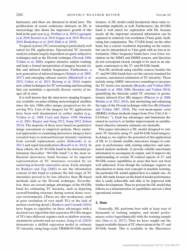
The imagery in MINT includes observations of TCs

ranging in intensity from 15 to 160 kt. Because of the

intensity distributions of the typical TC life cycle, the

images are most frequently of the tropical depression

stage, then decline in number with increasing intensity.

We filter the dataset for three factors to prevent mis-

leading structural patterns: 1) TCs must be centered

over water, 2) scan coverage must be .65% of the

image box, and 3) the TC must not be labeled as ‘‘extra-

tropical transition’’ in the records. The images are crop-

ped to a width of 3.68 (;400 km) in both dimensions and

sampled to 0.058 (;5 km) resolution using nearest-

neighbor interpolation, making the working images

72 3 72 pixels in size.

A standard measure of TC intensity is the maximum

sustained wind (MSW), defined as the TC’s maximum

1-min sustained wind at 10m above the surface. Here

we use the estimated MSW from the best track records

of two sources: 1) the HURDAT2 database, which uses

estimates from the National Hurricane Center for the

North Atlantic or east Pacific basins, and the Central

Pacific Hurricane Center in the central Pacific basin

(Landsea et al. 2013); and 2) the Joint Typhoon Warning

Center best tracks in thewest Pacific, north IndianOcean,

and Southern Hemisphere (Chu et al. 2002). Each image

is assigned the best track MSWmatching the image time

TABLE 1. Satellite microwave instruments used in the MINT dataset.

Satellitea Instrument Frequency (GHz) Orbit Footprint (km 3 km) Reference

DMSP F8–F15 SSM/I 37.0, H 85.5, H Polar, sunsynchronous 37 3 28, 16 3 14 Raytheon Systems

Company (2000)

DMSP F16–F18 SSMIS 37.0, H 91.7, H Polar, sunsynchronous 45 3 28, 14 3 13 Kunkee et al. (2008)

TRMM TMI 37.0, H 85.5, H Equatorial, between

388S and 388N16 3 9, 7 3 5 Kummerow et al. (1998)

Aqua AMSR-E 36.5, H 89.0, H Polar, sunsynchronous 14 3 8, 6 3 4 NASA MSFC (2001)

a Acronyms/abbreviations: DMSP: Defense Meteorological Satellites Program, SSM/I: Special Sensor Microwave Imager, H: Horizontal

polarization, SSMIS: Special Sensor Microwave Imager/Sounder, TRMM: Tropical Rainfall Measuring Mission, TMI: TRMM Micro-

wave Imager, AMSR-E: Advanced Microwave Scanning Radiometer—Earth Observing System.

FIG. 1. Histogram of TC passive microwave image samples used in the model training.

JUNE 2019 W IMMERS ET AL . 2263

Unauthenticated | Downloaded 10/17/21 12:01 AM UTC

through linear interpolation. Note that using these best

track MSW estimates as ‘‘truth’’ is not optimal because

only a minority of these values has in situ confirmation;

however, this was necessary for maintaining a large

sample size of relatively homogeneous data. Analysis

issues stemming from the limitations in this dataset are

discussed in sections 5 and 6.

The standard practice for DL modeling is to split

the dataset into independent training, validation, and

‘‘testing’’ components. Here, ‘‘validation’’ has a different

meaning than usual for atmospheric science applica-

tions. It denotes an independent confirmation of model

accuracy during training. By contrast, the ‘‘testing’’ com-

ponent uses independent data and ultimately measures

the accuracy of the finished model. In this study we use

year 2010 data for the validation, years 2007 and 2012

data for testing, and all other years for training (Fig. 1,

Table 2). These years were selected because 1) later

years have more data and better best track estimates;

and 2) 2007, 2010, and 2012 have an adequate amount

of category 4–5 aircraft reconnaissance observations for

statistical evaluation. In addition, we create a so-called

‘‘balanced’’ dataset during training and validation, which

is composed of duplicated data at lesser-sampled in-

tensities so that all values of MSW are equally repre-

sented. For example, referring to respective sample

sizes in Fig. 1, the 30-kt bin remains as is, the 50-kt bin is

duplicated 2.1 times and the 160-kt bin is duplicated

1233 times. Furthermore, all imagery including the

duplicated imagery is varied through rotation and off-

setting as described in section 4. This approach is nec-

essary for the model to assign equal importance to all

TC intensities during training, and is common practice

in CNN training in order to prevent the model from

inherently increasing its skill with the greater-sampled

image types at the expense of the lesser-sampled image

types. However, the testing dataset does not need to be

balanced in this way, because the determination of

model skill follows a different (and more conventional)

approach.

3. Deep learning model: DeepMicroNet

The common Deep Learning network model applied

to image data, and used here, is a convolutional neural

network (CNN). A full tutorial on how CNNs operate

TABLE 2. Dataset sizes and characteristics.

Dataset N N (balanced) Years Basins

Training 52 753 240 746 1987–2006, 2008–09, 2011 Global

Validation 3016 13 041 2010 Global

Testing 6705 — 2007, 2012 Global

Testing (recon only) 404 — 2007, 2012 North Atlantic,

east Pacific

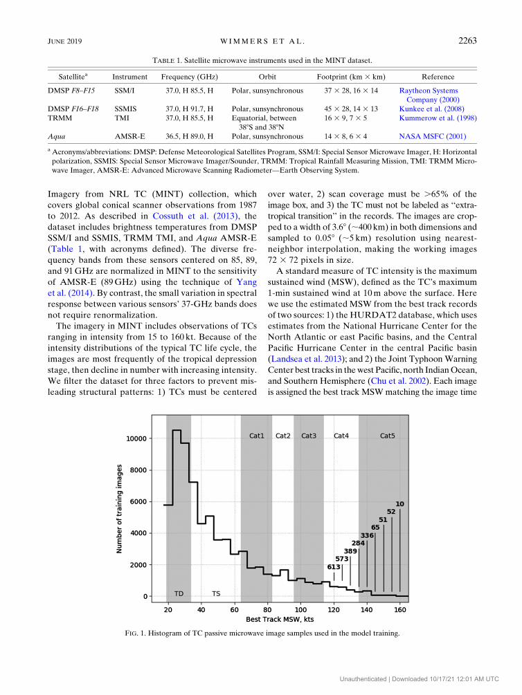
FIG. 2. Simplified diagram of the standard convolutional neural network architecture, with terms explained in section 3.

2264 MONTHLY WEATHER REV IEW VOLUME 147

Unauthenticated | Downloaded 10/17/21 12:01 AM UTC

is beyond the scope of this paper, but for background we

recommend O’Shea and Nash (2015) and Deshpande

(2016) to reach a more complete understanding of the

terminology and methods used in this section. Dieleman

et al. (2015) also provide an excellent demonstration of

CNNs to the problem of galaxy classification along with a

thorough introduction of the concepts. In broad terms, a

CNN operates by applying two- or three-dimensional

‘‘filters’’ that scan an input image for elemental features

of relevance to the task, and then producing an in-

termediate product with multiple channels (‘‘feature

maps’’) of information in a third dimension (Fig. 2),

while maintaining the spatial structure of the image

information. This operation repeats many times with

each operation producing a new intermediate layer.

The progressively larger-scale image representation of

successive layers allows them to work at a higher level

of abstraction than the layer before. Layer-wise oper-

ations include convolution (to resolve relevant patterns

and shapes), pooling (to reduce the size of the informa-

tion), normalization (to prevent runaway weighting) and

activation (to introduce nonlinearity with simple signal

gates). In the final stages of a CNN model, this three-

dimensional intermediate product is then remapped

as a flat, one-dimensional array of nodes. This array

connects to a set of ‘‘fully connected’’ layers and then

to the output layer. Together, all these layers make up

an architecture of interconnected nodes, or ‘‘neurons,’’

found in the convolutional filters and layered connec-

tions. Each connection between neurons is calibrated

with weights and offsets during the training of the

model in order to produce an optimized output. The

primary function of the convolution and pooling seg-

ment, shown in Fig. 2, is for feature identification,

whereas the primary function of the fully connected

segment is classification. Although normalization and

activation are not explicitly shown in this diagram, they

are applied throughout the model.

The particular architecture of our CNN model, called

‘‘DeepMicroNet’’ (Table 3), is loosely based on theAlexNet

design for image classification (Girshick et al. 2014). The

‘‘stride’’ column accounts for how the intermediate

TABLE 3. DeepMicroNet model architecture.a

Layer Type Filter size Stride Activation Feature maps Feature size

In Input — — — 1 or 2b 64 3 64

C1 Convolution 5 3 5 1 Leaky ReLU 16 64 3 64

P1 Max poolingc 2 3 2 2 — 16 32 3 32

BN1 Batch normalization — — — 16 32 3 32

C2 Convolution 5 3 5 1 Leaky ReLU 32 32 3 32

P2 Max pooling 2 3 2 2 — 32 16 3 16

BN2 Batch normalization — — — 32 16 3 16

C3 Convolution 3 3 3 1 Leaky ReLU 64 16 3 16

C4 Convolution 3 3 3 1 Leaky ReLU 64 16 3 16

C5 Convolution 3 3 3 1 Leaky ReLU 64 16 3 16

P5 Max pooling 2 3 2 2 — 64 8 3 8

C6 Convolution 3 3 3 1 Leaky ReLU 128 8 3 8

C7 Convolution 3 3 3 1 Leaky ReLU 128 8 3 8

C8 Convolution 3 3 3 1 Leaky ReLU 128 8 3 8

P8 Max pooling 2 3 2 2 — 128 4 3 4

C9 Convolution 3 3 3 1 Leaky ReLU 256 4 3 4

C10 Convolution 3 3 3 1 Leaky ReLU 256 4 3 4

C11 Convolution 3 3 3 1 Leaky ReLU 256 4 3 4

P11 Max pooling 2 3 2 2 — 512 2 3 2

C12 Convolution 3 3 3 1 Leaky ReLU 512 2 3 2

C13 Convolution 3 3 3 1 Leaky ReLU 512 2 3 2

C14 Convolution 3 3 3 1 Leaky ReLU 512 2 3 2

C15 Convolution 2 3 2 2 Leaky ReLU 1024 1 3 1

FC1 Fully connected — — Leaky ReLU — 1000

FC2 Fully connected — — Leaky ReLU — 200

Out Fully connected — — Softmax — 29

a Terms—Filter Size: Size of the convolutional filter, Stride: Spacing of the convolutional/pooling filter application, Activation: Nonlinear

‘‘signal gate’’ processing method following the layer process, Feature Maps: Layer depth of the product of convolution/pooling/etc.,

Feature Size: Row3 column size of the product of convolution/pooling/fully connected layer, LeakyReLU: ‘‘LeakyRectified LinearUnit’’

(a type of activation function that prevents neuron saturation in deep networks), Max Pooling: Calculation a local maximum of data within

feature maps (here in a 2 3 2 window, stepped by a stride of 2) in order to efficiently condense the information to fewer variables.b 1 if one channel only, 2 if 37 and 89GHz.c Steps that reduce the data size within the CNN are indented.

JUNE 2019 W IMMERS ET AL . 2265

Unauthenticated | Downloaded 10/17/21 12:01 AM UTC

layers are subsampled. The ‘‘Leaky ReLU’’ activation is a

fairly rapid and streamlined activation function (signal gate)

among several available options. The final signals from the

model (‘‘scores’’) are then processed with the softmax

function S, which normalizes the output into a probability

density function (PDF) in the output dimension:

S(yi)5

eyi

�j

eyj, (1)

where eyi is the exponent of the raw score coming from

the CNN model for the classification i (such as 70, 75 kt,

etc.), and the denominator is the sum of the terms for all

classifications.

This model design generally follows the best practices

of simple CNN construction. Specifically, convolutional

filter sizes are kept small in order to follow the ‘‘narrow

and deep’’ approach rather than ‘‘wide and shallow’’

because larger filters tend to increase computational

time. The addition of a pooling step is typical at every

other layer in the beginning in order to reduce di-

mensionality of the data early in processing, and then less

frequently afterward. Themanyparameters (overall number

of layers, feature map number, fully connected neuron

number, filter size and stride) were optimized by trial and

error, but are near the typical values for similarCNNmodels.

Most CNN architecture is designed to make classifi-

cations that have little to no interrelationship, such as

‘‘car,’’ ‘‘pedestrian,’’ and ‘‘street sign,’’ and aCNNmodel

is optimized to simply maximize the probability of cor-

rect classification. However, it would be unsuitable to

adopt this strict convention to the TC intensity problem

because then the model would not understand that

‘‘70 kt’’ is a close approximation of ‘‘75 kt,’’ and so on.

An alternative approach is to produce a scalar value

as output (such as MSW) and optimize the model by

minimizing the least squares error with the training

data. However, it would be less helpful to end users

to supply just a MSW value as output with no context.

Instead, we take the following unique approach that

retains the probabilistic output of the classification ap-

proach along with a built-in consideration for the re-

lationship between similar values of MSW. Here, the

‘‘truth’’ value of MSW is treated as a weighted distri-

bution ofMSWvalues in rough accordance with the best

track uncertainty reported by Torn and Snyder (2012).

For instance, one case of a best track value of ‘‘70 kt’’ is

treated in this model as a range of values {60, 65, 70, 75,

80 kt} weighted by importance with the input filterW 5{0.10, 0.23, 0.34, 0.23, 0.10}. The filter is applied univer-

sally, except that at the edges of the MSW range the

filter is truncated and renormalized accordingly. This

approach has the advantage of smoother and more

robust guidance toward the lowest error during model

training without the complicating influence of more

distant values of MSW, which can happen in a least-

squared error approach.

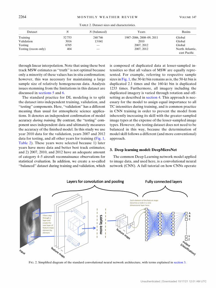
FIG. 3. Learning curve for the two-channel DeepMicroNet

model. Training progresses at 1000 images per step, hence the

number of training steps per epoch is 240 746/1000 5 241. The

model state at the point ‘‘Best loss’’ is the state used in this study.

TABLE 4. Training hyperparameter values in DeepMicroNet.

Hyperparameter Value

Batch size 1000

Learning rate 0.006

Learning rate decay 0.93 over 500 batch steps

Momentum 0.9

Dropout rate on fully

connected layers

50%

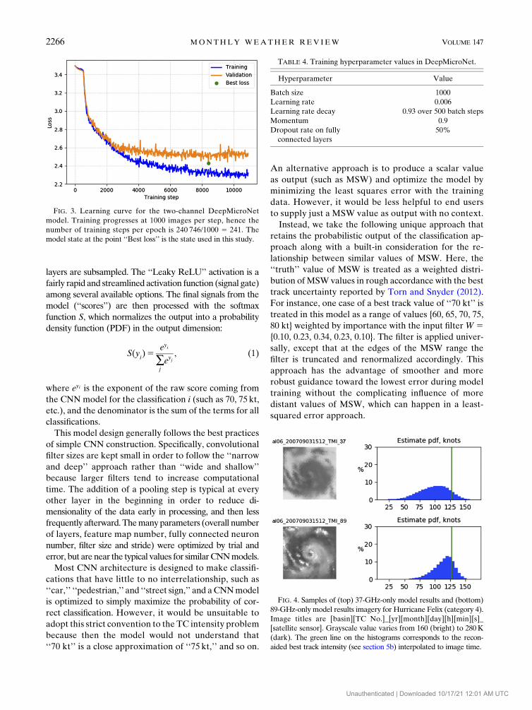
FIG. 4. Samples of (top) 37-GHz-only model results and (bottom)

89-GHz-only model results imagery for Hurricane Felix (category 4).

Image titles are [basin][TC No.]_[yr][month][day][h][min][s]_

[satellite sensor]. Grayscale value varies from 160 (bright) to 280K

(dark). The green line on the histograms corresponds to the recon-

aided best track intensity (see section 5b) interpolated to image time.

2266 MONTHLY WEATHER REV IEW VOLUME 147

Unauthenticated | Downloaded 10/17/21 12:01 AM UTC

We have set up 33 possible classifications of best track

MSW values from 10 to 170kt, stepped by 5kt. Note that

during training we use duplicates of the 20-kt data to train

the 10- and 15-kt classifications, and likewise the 165- and

170-kt classifications are trained with copies of the 160-kt

data.We developed this edge-buffer approach in order to

allow PDFs to spread naturally around the actual limits of

20 and 160kt for more accurate training. This would ad-

mittedly fail to train the exceedingly rare cases of.160-kt

intensity, but this issue is not important for the proof-of-

concept purpose of this study.

The DeepMicroNet model is built in Python with the

Tensorflow library (Abadi et al. 2016), which was se-

lected for its speed and versatility. The model training

runs on a server with 3 Intel Haswell CPUs, and always

in GPU-enabled mode employing one GeForce GTX

1080 8GB video card.

4. Model training

Model training in a DL architecture begins with a

random initialization of weights between model nodes,

FIG. 5. (a) Intensity error (RMSE) according to best trackMSW for the three model versions

labeled in the legend, and (b) average standard deviation of the PDFs according to best

track MSW.

JUNE 2019 W IMMERS ET AL . 2267

Unauthenticated | Downloaded 10/17/21 12:01 AM UTC

and then iteratively improves performance by shaping

the network toward an optimal fit to the training dataset

through stochastic gradient descent. This is very similar

to the approach of adjusting the state of an atmo-

spheric model with observational data and converg-

ing on a new solution with gradient descent along an

adjoint model (Thacker 1988; Errico 1997). Here, the

goal of the model is to reach optimal performance by

minimizing the loss function, defined as the ‘‘cross

entropy’’ of the output PDFs:

loss521

N�N

i50

W(yi) logS(y0i) , (2)

where N is the number of classifications, W is the input

filter applied to the ‘‘truth’’ classification yi and S(y0i) isthe softmax function applied to the model output. The

term ‘‘cross entropy’’ is appropriate here because it

parallels the mathematics of entropy along various

states of energy in statistical mechanics.

To reduce overfitting during model training, we also

employed three dataset augmentation techniques to

the training data. First, the positions of the training

images are randomly shifted 24 to 4 pixels in each di-

rection (620 km, to match the uncertainty in best

track positions) and cropped to 64 pixels in size from

the original 72-pixel template. Second, the images are

randomly flipped with 50% probability along the hor-

izontal axis so that Northern and Southern Hemisphere

configurations are represented equally, and so that the

model is rotationally invariant. Third, the images are

rotated randomly up to 408 in either direction. The

training process works through many iterations of the

dataset so that many combinations of offset, north/

south orientation and rotation are represented for each

image.

FIG. 6. Samples of (left) 37-GHz, (middle) 89-GHz imagery, and (right) corresponding

DeepMicroNet probabilisticMSWoutput for tropical depression strength TCs. Image titles are

[basin][TC No.]_[yr][month][day][h][min][s]_[satellite sensor]. Grayscale value varies from

160 (bright) to 280K (dark). The green line on the histograms corresponds to the recon-aided

best track intensity interpolated to image time. (top) A typical model underestimate of in-

tensity, and (bottom) a typical overestimate of intensity.

2268 MONTHLY WEATHER REV IEW VOLUME 147

Unauthenticated | Downloaded 10/17/21 12:01 AM UTC

The training process for the two-channel model (dis-

cussed in section 5b) converges to an optimum solu-

tion after 34 iterations, or ‘‘epochs,’’ of the training data

(Fig. 3). This lasted about 3 h on our system. Note that

the optimum solution is the state in which the validation

dataset, not the training dataset, has the lowest com-

puted loss, which is standard practice for model devel-

opment in machine learning. Further model training

generally results in overfitting to the training dataset.

Finally, the training hyperparameters, which con-

trol the learning process of the training stage (and are

rather esoteric to nonmachine learning researchers),

were finalized by recursively searching for the opti-

mum hyperparameter value that efficiently mini-

mized the loss, one at a time. These values are shared

in Table 4 simply to help with the reproducibility of

the model.

5. Independent case testing of the model

This section primarily describes the results of in-

dependent model testing and highlights the most

important features. For better clarity, the further discus-

sion of their meaning follows in the next section.

a. Comparative testing of 37- and 89-GHz channels

To understand the relative value of each channel to

estimating TC intensity, the DeepMicroNet model was

run in three versions: 1) using only the 37-GHz channel,

2) using only the 89-GHz channel, and 3) using both

channels. Because model performance varies slightly in

each training session, we trained the model three times

for each scenario and selected the best performer (with

respect to the validation dataset) to represent the group.

An example of 37-GHz-only and 89-GHz-only per-

formance (Fig. 4) shows how the model produces esti-

mates from image input. The probability density

function (PDF) is much wider for the 37-GHz-only

scenario than for the 89-GHz-only scenario, due to

lower precision in the model’s ability to train on the

data, and resulting in higher uncertainty in the model’s

intensity estimate.

Full results clearly show that the 89-GHz-onlymodel has

lower error and lower uncertainly than the 37-GHz-only

FIG. 7. As in Fig. 6, but for tropical storm strength TCs.

JUNE 2019 W IMMERS ET AL . 2269

Unauthenticated | Downloaded 10/17/21 12:01 AM UTC

model overall (Fig. 5). The 2-channel model, on the

other hand, slightly outperforms the 89-GHz-only model,

but shows no substantial difference in precision (width

of PDFs).Evidently the 89-GHz band supplies the more

relevant information to TC intensity, and the model uses

the 37-GHz band in a similar but less impactful way.

Only amarginal amount of information from the 37-GHz

band contributes uniquely to the 2-channel model, with

the largest improvement coming in the category 5

intensity range. However, it is difficult to generalize

this difference because of the small sample size for

category 5. Overall, the improvement is enough to

justify limiting the remaining model evaluation to

only the two-channel version of DeepMicroNet going

forward.

b. Model performance

The following describes a two-channel model se-

lected as the best of 12 runs based on performance

using the pretesting (validation) data. (The model was

found to perform differently on each run due to ran-

dom initialization and stochastic iterations toward

a local optimum.) Model performance is evaluated

against both the best track record and a more limited

dataset of best track intensity estimates within 3 h

from an aircraft reconnaissance observation (here-

after the ‘‘recon-aided best track’’). The first part

evaluates the ability of the model to replicate the best

track intensity estimates, whereas the second part

evaluates the ability of the model to estimate more

accurate recon-aided best track intensity. These two

comparisons are different insofar as the best track has

errors and biases of its own, largely due to the pre-

dominant influence of the Dvorak technique on the

best track record.

A small, representative sample from the 6705 test cases

demonstrates the variety of model output (Figs. 6–12).

(This sample was selected from the recon-aided dataset

of the east Pacific and North Atlantic basins in order to

insure an accurate ‘‘truth’’ MSW value, but we have

found that the following analysis applies to all basins.)

The figures are ordered by Saffir–Simpson hurricane

wind scale category, and each figure shows one un-

derestimation of MSW (top row), two high-accuracy

FIG. 8. As in Fig. 6, but for category 1 strength TCs.

2270 MONTHLY WEATHER REV IEW VOLUME 147

Unauthenticated | Downloaded 10/17/21 12:01 AM UTC

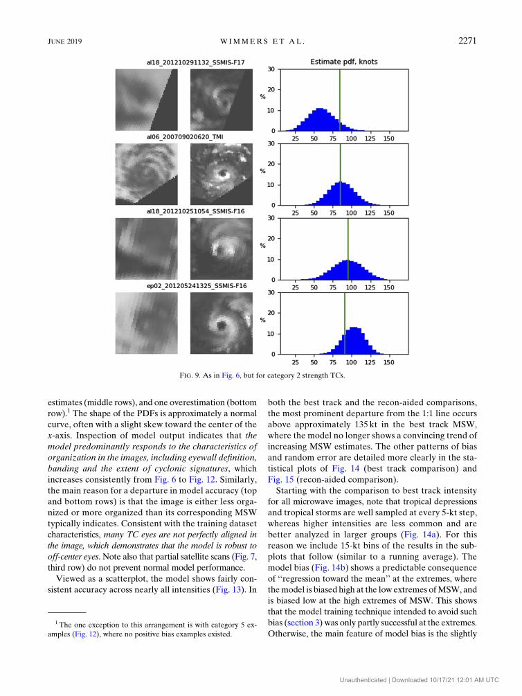
estimates (middle rows), and one overestimation (bottom

row).1 The shape of the PDFs is approximately a normal

curve, often with a slight skew toward the center of the

x-axis. Inspection of model output indicates that the

model predominantly responds to the characteristics of

organization in the images, including eyewall definition,

banding and the extent of cyclonic signatures, which

increases consistently from Fig. 6 to Fig. 12. Similarly,

the main reason for a departure in model accuracy (top

and bottom rows) is that the image is either less orga-

nized or more organized than its corresponding MSW

typically indicates. Consistent with the training dataset

characteristics, many TC eyes are not perfectly aligned in

the image, which demonstrates that the model is robust to

off-center eyes. Note also that partial satellite scans (Fig. 7,

third row) do not prevent normal model performance.

Viewed as a scatterplot, the model shows fairly con-

sistent accuracy across nearly all intensities (Fig. 13). In

both the best track and the recon-aided comparisons,

the most prominent departure from the 1:1 line occurs

above approximately 135 kt in the best track MSW,

where the model no longer shows a convincing trend of

increasing MSW estimates. The other patterns of bias

and random error are detailed more clearly in the sta-

tistical plots of Fig. 14 (best track comparison) and

Fig. 15 (recon-aided comparison).

Starting with the comparison to best track intensity

for all microwave images, note that tropical depressions

and tropical storms are well sampled at every 5-kt step,

whereas higher intensities are less common and are

better analyzed in larger groups (Fig. 14a). For this

reason we include 15-kt bins of the results in the sub-

plots that follow (similar to a running average). The

model bias (Fig. 14b) shows a predictable consequence

of ‘‘regression toward the mean’’ at the extremes, where

themodel is biased high at the low extremes ofMSW, and

is biased low at the high extremes of MSW. This shows

that the model training technique intended to avoid such

bias (section 3) was only partly successful at the extremes.

Otherwise, the main feature of model bias is the slightly

FIG. 9. As in Fig. 6, but for category 2 strength TCs.

1 The one exception to this arrangement is with category 5 ex-

amples (Fig. 12), where no positive bias examples existed.

JUNE 2019 W IMMERS ET AL . 2271

Unauthenticated | Downloaded 10/17/21 12:01 AM UTC

(but significantly) positive values in the middle range

(30–110 kt), which we will consider along with the bias

against recon-aided best track later on. Predictably, the

modes of the PDFs have less bias than the means be-

cause the means are more sensitive to skew, but it is

worthwhile to analyze the statistics of the mean and

mode together because the mean has less error away

from the extremes of MSW (Fig. 14c). However, error

from negative bias clearly dominates the model RMSE

in the category-5 range of intensities for both the mode

and mean. Likewise, positive bias is also significant for

the RMSE, but less extreme, at the tropical depression

(TD)–tropical storm (TS) range.

All the statistics up to this point evaluate the accuracy

of a single center value in the PDF distribution, but what

about the distribution itself? Here the reliability of the

PDF is measured by the percentage of samples whose

best track MSW fall inside the innermost 50% of the

PDFs (Fig. 14d). The percentage is above 50% if the

PDFs are too wide and below 50% if the PDFs are too

narrow. For most TC intensities the value is close to

50%, indicating that the PDF distributions accurately

reflect the true uncertainty of the model MSW estimate.

Only at category 5 intensities are the values too low,

confirming that here the distributions do not extend

far enough.

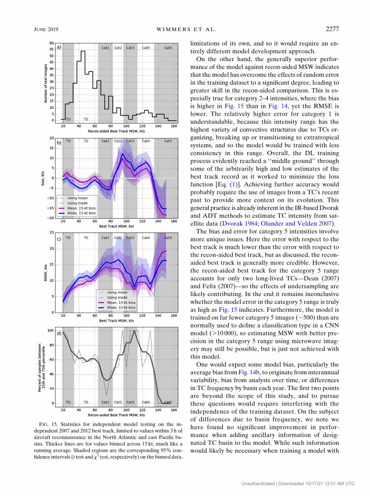
Recon-aided best track intensities are fewer in num-

ber by more than an order of magnitude (Fig. 15a), but

still numerous enough that it is at least possible to dis-

cuss the trends according to the Saffir-Simpson hurri-

cane wind scale category. In the TS–category 1 range,

the model is biased slightly low, and then biased high at

categories 2–4 (Fig. 15b). The strong negative bias at the

category 5 range is similar to the best track analysis

above, but here it is even more extreme. RMS error

(Fig. 15c) generally varies more with TC intensity, with

one relative maximum around categories 1–2, and an-

other maximum at category 5. Note also that error is

consistently lower for the model-derived mean than

for the mode, likely because of its lower magnitude of

bias (except for category 5). Finally, the evaluation of

the model PDF (Fig. 15d) has well over 50% of the

FIG. 10. As in Fig. 6, but for category 3 strength TCs. Note that themost significant low bias case

in this range (top row) has a mean error of only 25.4 kt.

2272 MONTHLY WEATHER REV IEW VOLUME 147

Unauthenticated | Downloaded 10/17/21 12:01 AM UTC

observations falling within the inner 50% of the model

PDF for most intensities. This reveals that over most

intensities the model PDF is too wide, or in other

words, the model intensity estimate is actually more

precise than its PDF indicates.

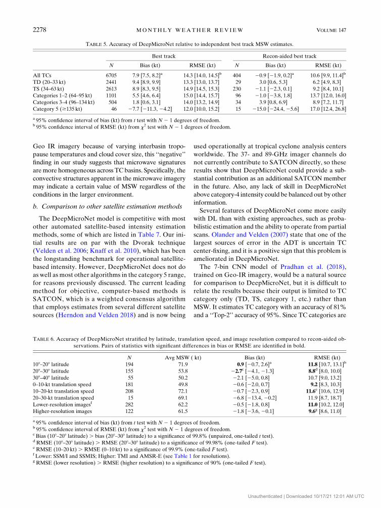
Error statistics from Figs. 14 and 15 using themean of

PDF values are summarized in Table 5.

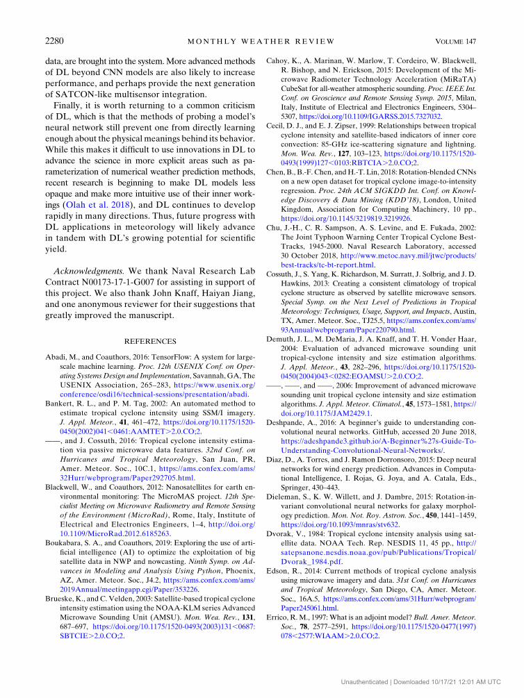
c. Sensitivity of the model to common TC variables

A further examination of the model sensitivity to lati-

tude, translation speed, and image resolution applied to

recon-aided observations is provided in Table 6. Pairs of

statistics with significant differences in bias or RMSE are

identified in bold. However, the groupings according to

latitude and translation speed have substantial differ-

ences in average MSW, which indicates a serious poten-

tial for cross correlation between model error and TC

intensity. For example, the RMSE is significantly lower in

each of the groupings for latitude and translation speed

that have lower MSW (and lower MSW alone corre-

sponds to lower RMSE as in Fig. 15c). A larger sample

of observations would be necessary to control for this

influence, and so these results for latitude and trans-

lation speed must be taken with caution.

The most counterintuitive result in this table is the

similarity in bias with translation speed from 0–10 to

10–20 kt (20.6 and 20.7 kt, respectively). This result

strongly suggests that the model has a mechanism for

incorporating the effects of translation speed within

0–20 kt. Whether this result persists in the (rather ex-

treme) 20–30-kt range is not certain because of the

small sample size (N 5 15).

Finally, the groupings by image resolution are the

most likely to be sampled fairly, as their average MSW

values differ by less than 1 kt. The RMSE is larger when

applied to lower-resolution images than when applied

to higher-resolution images to a confidence of 90%.

Moreover, the reduction in RMSE from 11.0 kt (lower

resolution) to 9.6 kt (higher resolution) is a substantial

improvement that approaches the accuracy of current

state-of-the-art methods (section 6b). Given the sig-

nificance of this result, it is reasonable to ask whether

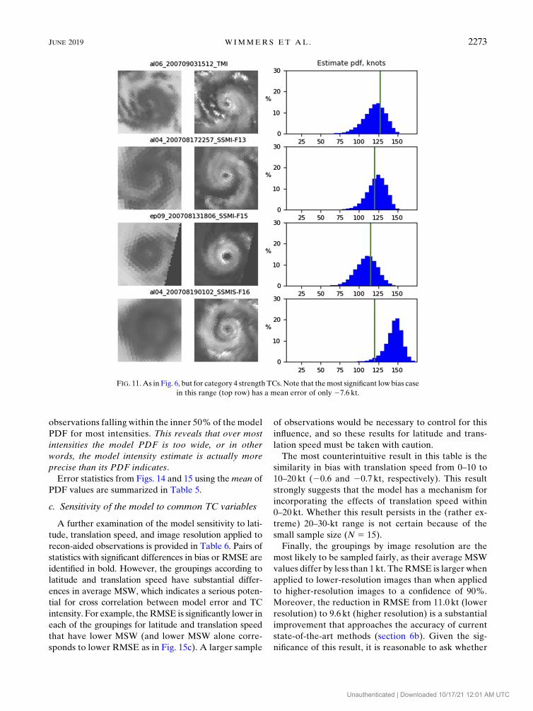
FIG. 11. As in Fig. 6, but for category 4 strength TCs. Note that themost significant low bias case

in this range (top row) has a mean error of only 27.6 kt.

JUNE 2019 W IMMERS ET AL . 2273

Unauthenticated | Downloaded 10/17/21 12:01 AM UTC

the 37-GHz channel is less impactful in DeepMicroNet

simply because of its lower resolution in most of the

training dataset, or because of something more fun-

damental to what it depicts? The lower precision of the

37-GHz-based model in estimating MSW (wider PDFs,

Fig. 4) at both high resolution and low resolution strongly

suggests that the reason is fundamental to the 37-GHz

channel. The reason for this is likely that the 37-GHz

signal captures low-level features (warm rain and shal-

low convection), whereas the 89-GHz signal captures

more of the deep convection associated with the eyewall

and inner rainbands that relate more to MSW.

d. Results of models trained to forecast TC intensity

After optimizing the CNN model to estimate MSW

at the time of the image, it is a simple task to retrain the

model with best track MSW forward in time, so that

the resulting model estimates the future MSW. When

comparing to the futureMSW from all best track cases,

the same sample was used as previously, omitting only

those with forecasts that were later than the latest best

track point. When comparing to recon-aided best track

MSW, the same sample was used as before, and was not

adjusted for the differing availability of reconnaissance

observations at the forecast time. This was done in order

to keep the sample observations consistent in each ver-

sion of the model, in spite of the trade-off of further un-

certainty in the ‘‘truth’’MSWvalue.Aswith the experiment

in section 5a, we used three model runs for each forecast

time and selected the best one to represent the results

for that time. This insures a more authentic trend with

time because it is less influenced by random error.

Results show a steady increase in model error at fore-

casting best track MSW beyond 6h, and an abrupt in-

crease in error at forecasting recon-aided MSW beyond

6 h (Fig. 16). However, in both cases the models had

slightly more skill at 16 h than at the exact time of the

satellite observation, which was also found with the

statistical prediction scheme of Jiang et al. (2019) based

on TRMM TMI imagery. This improvement in skill

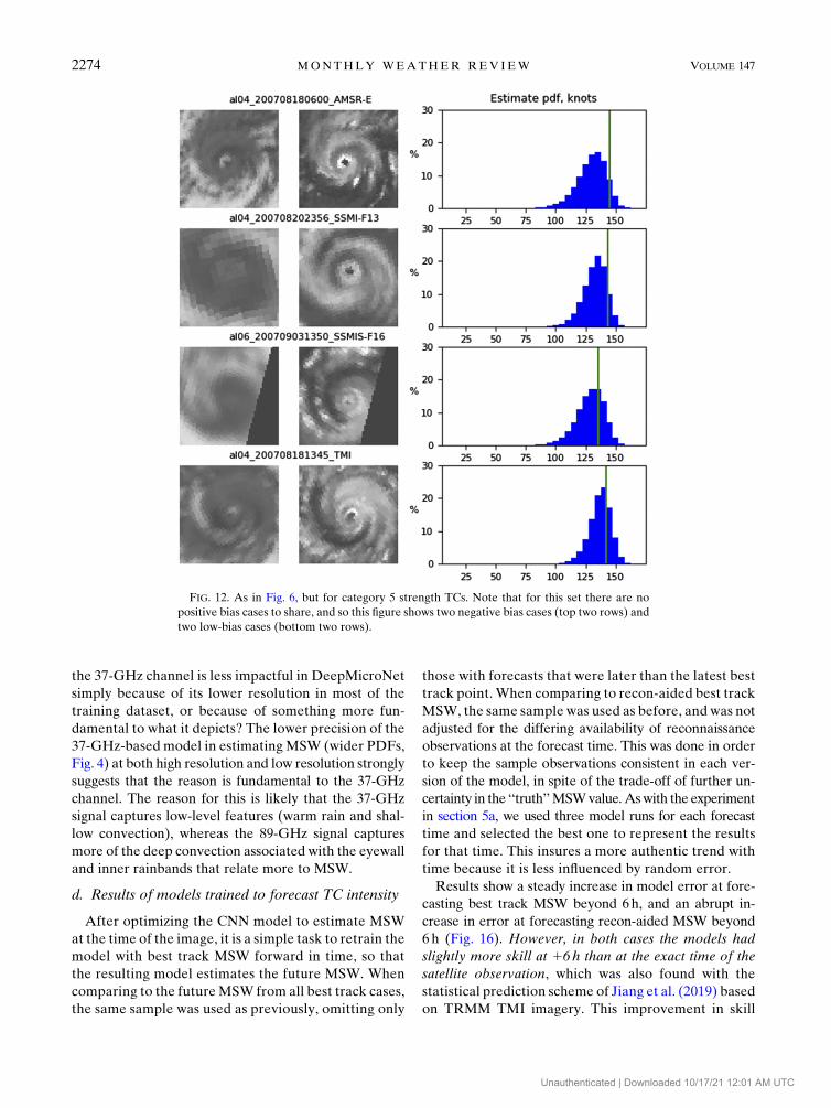
FIG. 12. As in Fig. 6, but for category 5 strength TCs. Note that for this set there are no

positive bias cases to share, and so this figure shows two negative bias cases (top two rows) and

two low-bias cases (bottom two rows).

2274 MONTHLY WEATHER REV IEW VOLUME 147

Unauthenticated | Downloaded 10/17/21 12:01 AM UTC

FIG. 13. (a) Heat map scatterplot of independent model-estimated MSW for 2007 and 2012 vs

global best track; (b) as in (a), but limited to recon-observed times/locations.

JUNE 2019 W IMMERS ET AL . 2275

Unauthenticated | Downloaded 10/17/21 12:01 AM UTC

at16 h makes sense in light of the time required for the

latent heat release from deep convection in a TC (ev-

ident in the 89-GHz imagery) to affect the gradient

balance and surface pressure/wind.

The stark difference in error between best track and

recon-aided cases beyond 6h is not easily accounted for,

but factors that could explain the difference include: a

lower temporal variability in the full best track MSW

dataset due to lack of reconnaissance, the higher oc-

currence of landfall shortly after reconnaissance (lead-

ing to higher MSW variability), and the higher average

variability in MSW in the recon-aided dataset due to its

higher average MSW. In other words, the best track

MSW is a more homogeneous dataset for testing accu-

racy with forecast time, indicating that this trend is ac-

tually better represented with the best track than with

the recon-aided dataset.

6. Discussion

a. Analysis of error

Perhaps counterintuitively, the DeepMicroNet model

performs better against TC intensity data informed by

reconnaissance (RMSE 5 10.6 kt) than against the kind

of best track data on which the model was directly

trained (RMSE5 14.3 kt). This is in spite of the fact that

the recon-aided best track has a higher proportion of

category 1, 2, and 5 TCs, which have higher model error

overall, and a lower proportion of TDs, which have

lower error. This result is very encouraging in light of

our understanding of the model training process. On

one hand, the model is expected to incorporate the

biases inherent in the best track training dataset. In-

deed, Knaff et al. (2010) observe that the Dvorak tech-

nique, which has a heavy influence on the best track,

exhibits a bias reaching as low as 24 to 26 kt where

MSW5 30–80 kt. Sheets and McAdie (1988) and Koba

et al. (1990, 1991) also note this tendency. Knaff et al.

(2010) also note a high bias in the Dvorak technique of

as much as 4 kt around MSW 5 100 kt, and then an-

other low bias of 28 kt at MSW 5 140 kt. All three of

these trends are captured very closely by our own com-

parison to recon-aided best track intensity (Fig. 15b). The

low-intensity bias in particular (aroundMSW5 30–80kt)

is often apparent in the microwave imagery as a system

with little convective organization but nonetheless high

surface winds, such as in Fig. 8 (top row). These biases

could be mitigated in the model by training on recon-

aided best track only, provided the sample size is large

enough for aDeep Learning environment. Overcoming

such a problem with sample size would be challenging,

given that the current training dataset has sample size

FIG. 14. Statistics for independent model testing on the in-

dependent 2007 and 2012 global best track. Thicker lines are for

values binned across 15 kt, much like a running average. Shaded

regions are the corresponding 95% confidence intervals (t test

and x2 test, respectively) on the binned data.

2276 MONTHLY WEATHER REV IEW VOLUME 147

Unauthenticated | Downloaded 10/17/21 12:01 AM UTC

limitations of its own, and so it would require an en-

tirely different model development approach.

On the other hand, the generally superior perfor-

mance of the model against recon-aided MSW indicates

that the model has overcome the effects of random error

in the training dataset to a significant degree, leading to

greater skill in the recon-aided comparison. This is es-

pecially true for category 2–4 intensities, where the bias

is higher in Fig. 15 than in Fig. 14, yet the RMSE is

lower. The relatively higher error for category 1 is

understandable, because this intensity range has the

highest variety of convective structures due to TCs or-

ganizing, breaking up or transitioning to extratropical

systems, and so the model would be trained with less

consistency in this range. Overall, the DL training

process evidently reached a ‘‘middle ground’’ through

some of the arbitrarily high and low estimates of the

best track record as it worked to minimize the loss

function [Eq. (1)]. Achieving further accuracy would

probably require the use of images from a TC’s recent

past to provide more context on its evolution. This

general practice is already inherent in the IR-basedDvorak

and ADT methods to estimate TC intensity from sat-

ellite data (Dvorak 1984; Olander and Velden 2007).

The bias and error for category 5 intensities involve

more unique issues. Here the error with respect to the

best track is much lower than the error with respect to

the recon-aided best track, but as discussed, the recon-

aided best track is generally more credible. However,

the recon-aided best track for the category 5 range

accounts for only two long-lived TCs—Dean (2007)

and Felix (2007)—so the effects of undersampling are

likely contributing. In the end it remains inconclusive

whether the model error in the category 5 range is truly

as high as Fig. 15 indicates. Furthermore, the model is

trained on far fewer category 5 images (;500) than are

normally used to define a classification type in a CNN

model (.10 000), so estimating MSW with better pre-

cision in the category 5 range using microwave imag-

ery may still be possible, but is just not achieved with

this model.

One would expect some model bias, particularly the

average bias fromFig. 14b, to originate from interannual

variability, bias from analysts over time, or differences

in TC frequency by basin each year. The first two points

are beyond the scope of this study, and to pursue

these questions would require interfering with the

independence of the training dataset. On the subject

of differences due to basin frequency, we note we

have found no significant improvement in perfor-

mance when adding ancillary information of desig-

nated TC basin to the model. While such information

would likely be necessary when training a model with

FIG. 15. Statistics for independent model testing on the in-

dependent 2007 and 2012 best track, limited to values within 3 h of

aircraft reconnaissance in the North Atlantic and east Pacific ba-

sins. Thicker lines are for values binned across 15 kt, much like a

running average. Shaded regions are the corresponding 95% con-

fidence intervals (t test and x2 test, respectively) on the binned data.

JUNE 2019 W IMMERS ET AL . 2277

Unauthenticated | Downloaded 10/17/21 12:01 AM UTC

Geo IR imagery because of varying interbasin tropo-

pause temperatures and cloud cover size, this ‘‘negative’’

finding in our study suggests that microwave signatures

aremore homogeneous across TC basins. Specifically, the

convective structures apparent in the microwave imagery

may indicate a certain value of MSW regardless of the

conditions in the larger environment.

b. Comparison to other satellite estimation methods

The DeepMicroNet model is competitive with most

other automated satellite-based intensity estimation

methods, some of which are listed in Table 7. Our ini-

tial results are on par with the Dvorak technique

(Velden et al. 2006; Knaff et al. 2010), which has been

the longstanding benchmark for operational satellite-

based intensity. However, DeepMicroNet does not do

as well as most other algorithms in the category 5 range,

for reasons previously discussed. The current leading

method for objective, computer-based methods is

SATCON, which is a weighted consensus algorithm

that employs estimates from several different satellite

sources (Herndon and Velden 2018) and is now being

used operationally at tropical cyclone analysis centers

worldwide. The 37- and 89-GHz imager channels do

not currently contribute to SATCON directly, so these

results show that DeepMicroNet could provide a sub-

stantial contribution as an additional SATCON member

in the future. Also, any lack of skill in DeepMicroNet

above category-4 intensity could be balanced out by other

information.

Several features of DeepMicroNet come more easily

with DL than with existing approaches, such as proba-

bilistic estimation and the ability to operate from partial

scans. Olander and Velden (2007) state that one of the

largest sources of error in the ADT is uncertain TC

center-fixing, and it is a positive sign that this problem is

ameliorated in DeepMicroNet.

The 7-bin CNN model of Pradhan et al. (2018),

trained on Geo-IR imagery, would be a natural source

for comparison to DeepMicroNet, but it is difficult to

relate the results because their output is limited to TC

category only (TD, TS, category 1, etc.) rather than

MSW. It estimates TC category with an accuracy of 81%

and a ‘‘Top-2’’ accuracy of 95%. Since TC categories are

TABLE 6. Accuracy of DeepMicroNet stratified by latitude, translation speed, and image resolution compared to recon-aided ob-

servations. Pairs of statistics with significant differences in bias or RMSE are identified in bold.

N Avg MSW ( kt) Bias (kt) RMSE (kt)

108–208 latitude 194 71.9 0.9 [20.7, 2.6]a 11.8 [10.7, 13.1]b

208–308 latitude 155 53.8 22.7c [24.1, 21.3] 8.8d [8.0, 10.0]

308–408 latitude 55 50.2 22.1 [25.0, 0.8] 10.7 [9.0, 13.2]

0–10-kt translation speed 181 49.8 20.6 [22.0, 0.7] 9.2 [8.3, 10.3]

10–20-kt translation speed 208 72.1 20.7 [22.3, 0.9] 11.6e [10.6, 12.9]

20–30-kt translation speed 15 69.1 26.8 [213.4, 20.2] 11.9 [8.7, 18.7]

Lower-resolution imagesf 282 62.2 20.5 [21.8, 0.8] 11.0 [10.2, 12.0]

Higher-resolution images 122 61.5 21.8 [23.6, 20.1] 9.6g [8.6, 11.0]

a 95% confidence interval of bias (kt) from t test with N 2 1 degrees of freedom.b 95% confidence interval of RMSE (kt) from x2 test with N 2 1 degrees of freedom.c Bias (108–208 latitude) . bias (208–308 latitude) to a significance of 99.8% (unpaired, one-tailed t test).d RMSE (108–208 latitude) . RMSE (208–308 latitude) to a significance of 99.98% (one-tailed F test).e RMSE (10–20 kt) . RMSE (0–10 kt) to a significance of 99.9% (one-tailed F test).f Lower: SSM/I and SSMIS; Higher: TMI and AMSR-E (see Table 1 for resolutions).g RMSE (lower resolution) . RMSE (higher resolution) to a significance of 90% (one-tailed F test).

TABLE 5. Accuracy of DeepMicroNet relative to independent best track MSW estimates.

Best track Recon-aided best track

N Bias (kt) RMSE (kt) N Bias (kt) RMSE (kt)

All TCs 6705 7.9 [7.5, 8.2]a 14.3 [14.0, 14.5]b 404 20.9 [21.9, 0.2]a 10.6 [9.9, 11.4]b

TD (20–33 kt) 2441 9.4 [8.9, 9.9] 13.3 [13.0, 13.7] 29 3.0 [0.6, 5.3] 6.2 [4.9, 8.3]

TS (34–63 kt) 2613 8.9 [8.3, 9.5] 14.9 [14.5, 15.3] 230 21.1 [22.3, 0.1] 9.2 [8.4, 10.1]

Categories 1–2 (64–95 kt) 1101 5.5 [4.6, 6.4] 15.0 [14.4, 15.7] 96 21.0 [23.8, 1.8] 13.7 [12.0, 16.0]

Categories 3–4 (96–134 kt) 504 1.8 [0.6, 3.1] 14.0 [13.2, 14.9] 34 3.9 [0.8, 6.9] 8.9 [7.2, 11.7]

Category 5 ($135 kt) 46 27.7 [211.3, 24.2] 12.0 [10.0, 15.2] 15 215.0 [224.4, 25.6] 17.0 [12.4, 26.8]

a 95% confidence interval of bias (kt) from t test with N 2 1 degrees of freedom.b 95% confidence interval of RMSE (kt) from x2 test with N 2 1 degrees of freedom.

2278 MONTHLY WEATHER REV IEW VOLUME 147

Unauthenticated | Downloaded 10/17/21 12:01 AM UTC

spaced by 13–30kt, a model such as DeepMicroNet with

an RMS error of 10.6kt would score at a similar level of

skill, though with higher precision. Further work would

be needed to show whether this difference in precision

also affects the inherent accuracy of the methods.

The recent DL regression model of Chen et al. (2018)

is also noteworthy here. They report an RMSE of 9.45 kt

compared to best track values for the west Pacific, east

Pacific, and North Atlantic basins. However, the mo-

del requires the Climate Prediction Center Morphing

(CMORPH, Joyce et al. 2004) rain rate imagery as in-

put, which is interpolated from microwave observations

from the past and future (CMORPHhas a 24-h latency).

Because of this latency and use of future data it is un-

fortunately not a near-real-time estimation like those in

Table 7. Regardless, it shows great promise in the combi-

nation of passive microwave imagery with other modes

of satellite observation.

7. Conclusions

By following a fairly standard recipe for CNN mod-

eling, this project has produced operational-quality TC

intensity estimates using satellite bands that have tra-

ditionally not played a major role in quantitative tech-

niques. The 89-GHz band in particular is shown to be a

first-order tool for intensity estimation—both in real

time and in forecasting to at least 6 h. Themodel’s ability

to find trends finer than the random error of the best

track and replicate the known best track biases shows

that further improvements are still possible. Addition-

ally, the low errors of this neural network technique

present a target for future analytical techniques to fur-

ther explain the precise mechanisms behind the 37- and

89-GHz bands’ relationship to intensity.

The technique has major implications for estimating

other aspects of TCs as well (e.g., radius of maximum

winds, rapid intensification, eyewall replacement cycles)

because the model design, and capabilities, would be

nearly the same for each of these applications. For some

tasks, only the training data and output classifications

would need to change. Furthermore, there is no reason

to believe that this level of performance is unique to 37-

and 89-GHz band imagery, as others have already

demonstrated a CNN application with Geo IR (Pradhan

et al. 2018; Chen et al. 2018). Even higher model accu-

racy and increased capabilities are all but certain when

more data sources, from satellite imagery to ancillary

FIG. 16. Error of the DeepMicroNet model trained on best track

intensity values at future times from 0 to 24 h, and tested on in-

dependent cases in 2007 and 2012. Shaded regions are the corre-

sponding 95% confidence intervals (x2 test).

TABLE 7. Comparable statistics of other satellite-based TC intensity estimation methods.

Method Data source Bias (kt)

RMSE (kt)

(all TCs)

RMSE (kt)

(categories 3–5) Referencesa

Dvorak technique Geo IR, Vis 2 to 28 10.5 12 Knaff et al. (2010)

Bias-corrected Dvorak

technique

Geo IR, Vis — 9.75 — Knaff et al. (2010)

Deviation angle variance Geo IR — 14–15 .15 Piñeros et al. (2008),Ritchie et al. (2012, 2014)

Advanced Dvorak

technique (ADT)

Geo IR ;0 11 13.3 Olander and Velden (2018)b

Warm core anomaly (CIRA) AMSU, ATMS 7 to 220 14 23 Demuth et al. (2004, 2006)

Warm core anomaly (CIMSS) AMSU, SSMIS, ATMS 22 12 13–14 Herndon and Velden (2018)b

Consensus approach

(SATCON)

ADT, AMSU, SSMIS,

ATMS

;0 8.9 9.2 Herndon and Velden (2018)b

Passive microwave TRMM TMI — 12.3 — Jiang et al. (2019)

Feature-based neural net SSM/I 85GHz — 19.8 — Bankert and Tag (2002)

Feature-based decision tree SSMI, SSMIS, TMI,

AMSR-E

— 11.9 — Bankert and Cossuth (2016)b

aWhere not explicitly stated in the reference paper, we approximate the values from tables and figures.b Nonrefereed source.

JUNE 2019 W IMMERS ET AL . 2279

Unauthenticated | Downloaded 10/17/21 12:01 AM UTC

data, are brought into the system.More advancedmethods

of DL beyond CNN models are also likely to increase

performance, and perhaps provide the next generation

of SATCON-like multisensor integration.

Finally, it is worth returning to a common criticism

of DL, which is that the methods of probing a model’s

neural network still prevent one from directly learning

enough about the physicalmeanings behind its behavior.

While this makes it difficult to use innovations in DL to

advance the science in more explicit areas such as pa-

rameterization of numerical weather prediction methods,

recent research is beginning to make DL models less

opaque and make more intuitive use of their inner work-

ings (Olah et al. 2018), and DL continues to develop

rapidly in many directions. Thus, future progress with

DL applications in meteorology will likely advance

in tandem with DL’s growing potential for scientific

yield.

Acknowledgments. We thank Naval Research Lab

Contract N00173-17-1-G007 for assisting in support of

this project. We also thank John Knaff, Haiyan Jiang,

and one anonymous reviewer for their suggestions that

greatly improved the manuscript.

REFERENCES

Abadi, M., and Coauthors, 2016: TensorFlow: A system for large-

scale machine learning. Proc. 12th USENIX Conf. on Oper-

ating SystemsDesign and Implementation, Savannah,GA, The

USENIX Association, 265–283, https://www.usenix.org/

conference/osdi16/technical-sessions/presentation/abadi.

Bankert, R. L., and P. M. Tag, 2002: An automated method to

estimate tropical cyclone intensity using SSM/I imagery.

J. Appl. Meteor., 41, 461–472, https://doi.org/10.1175/1520-

0450(2002)041,0461:AAMTET.2.0.CO;2.

——, and J. Cossuth, 2016: Tropical cyclone intensity estima-

tion via passive microwave data features. 32nd Conf. on

Hurricanes and Tropical Meteorology, San Juan, PR,

Amer. Meteor. Soc., 10C.1, https://ams.confex.com/ams/

32Hurr/webprogram/Paper292705.html.

Blackwell, W., and Coauthors, 2012: Nanosatellites for earth en-

vironmental monitoring: The MicroMAS project. 12th Spe-

cialist Meeting on Microwave Radiometry and Remote Sensing

of the Environment (MicroRad), Rome, Italy, Institute of

Electrical and Electronics Engineers, 1–4, http://doi.org/

10.1109/MicroRad.2012.6185263.

Boukabara, S. A., and Coauthors, 2019: Exploring the use of arti-

ficial intelligence (AI) to optimize the exploitation of big

satellite data in NWP and nowcasting. Ninth Symp. on Ad-

vances in Modeling and Analysis Using Python, Phoenix,

AZ, Amer. Meteor. Soc., J4.2, https://ams.confex.com/ams/

2019Annual/meetingapp.cgi/Paper/353226.

Brueske, K., and C. Velden, 2003: Satellite-based tropical cyclone

intensity estimation using the NOAA-KLM series Advanced

Microwave Sounding Unit (AMSU). Mon. Wea. Rev., 131,

687–697, https://doi.org/10.1175/1520-0493(2003)131,0687:

SBTCIE.2.0.CO;2.

Cahoy, K., A. Marinan, W. Marlow, T. Cordeiro, W. Blackwell,

R. Bishop, and N. Erickson, 2015: Development of the Mi-

crowave Radiometer Technology Acceleration (MiRaTA)

CubeSat for all-weather atmospheric sounding.Proc. IEEE Int.

Conf. on Geoscience and Remote Sensing Symp. 2015, Milan,

Italy, Institute of Electrical and Electronics Engineers, 5304–

5307, https://doi.org/10.1109/IGARSS.2015.7327032.

Cecil, D. J., and E. J. Zipser, 1999: Relationships between tropical

cyclone intensity and satellite-based indicators of inner core

convection: 85-GHz ice-scattering signature and lightning.

Mon. Wea. Rev., 127, 103–123, https://doi.org/10.1175/1520-

0493(1999)127,0103:RBTCIA.2.0.CO;2.

Chen, B., B.-F. Chen, andH.-T. Lin, 2018: Rotation-blended CNNs

on a new open dataset for tropical cyclone image-to-intensity

regression. Proc. 24th ACM SIGKDD Int. Conf. on Knowl-

edge Discovery & Data Mining (KDD’18), London, United

Kingdom, Association for Computing Machinery, 10 pp.,

https://doi.org/10.1145/3219819.3219926.

Chu, J.-H., C. R. Sampson, A. S. Levine, and E. Fukada, 2002:

The Joint Typhoon Warning Center Tropical Cyclone Best-

Tracks, 1945-2000. Naval Research Laboratory, accessed

30 October 2018, http://www.metoc.navy.mil/jtwc/products/

best-tracks/tc-bt-report.html.

Cossuth, J., S. Yang, K. Richardson, M. Surratt, J. Solbrig, and J. D.

Hawkins, 2013: Creating a consistent climatology of tropical

cyclone structure as observed by satellite microwave sensors.

Special Symp. on the Next Level of Predictions in Tropical

Meteorology: Techniques, Usage, Support, and Impacts, Austin,

TX, Amer. Meteor. Soc., TJ25.5, https://ams.confex.com/ams/

93Annual/webprogram/Paper220790.html.

Demuth, J. L., M. DeMaria, J. A. Knaff, and T. H. Vonder Haar,

2004: Evaluation of advanced microwave sounding unit

tropical-cyclone intensity and size estimation algorithms.

J. Appl. Meteor., 43, 282–296, https://doi.org/10.1175/1520-

0450(2004)043,0282:EOAMSU.2.0.CO;2.

——, ——, and ——, 2006: Improvement of advanced microwave

sounding unit tropical cyclone intensity and size estimation

algorithms. J. Appl. Meteor. Climatol., 45, 1573–1581, https://

doi.org/10.1175/JAM2429.1.

Deshpande, A., 2016: A beginner’s guide to understanding con-

volutional neural networks. GitHub, accessed 20 June 2018,

https://adeshpande3.github.io/A-Beginner%27s-Guide-To-

Understanding-Convolutional-Neural-Networks/.

Diaz, D., A. Torres, and J. Ramon Dorronsoro, 2015: Deep neural

networks for wind energy prediction. Advances in Computa-

tional Intelligence, I. Rojas, G. Joya, and A. Catala, Eds.,

Springer, 430–443.

Dieleman, S., K. W. Willett, and J. Dambre, 2015: Rotation-in-

variant convolutional neural networks for galaxy morphol-

ogy prediction.Mon. Not. Roy. Astron. Soc., 450, 1441–1459,

https://doi.org/10.1093/mnras/stv632.

Dvorak, V., 1984: Tropical cyclone intensity analysis using sat-

ellite data. NOAA Tech. Rep. NESDIS 11, 45 pp., http://

satepsanone.nesdis.noaa.gov/pub/Publications/Tropical/

Dvorak_1984.pdf.

Edson, R., 2014: Current methods of tropical cyclone analysis

using microwave imagery and data. 31st Conf. on Hurricanes

and Tropical Meteorology, San Diego, CA, Amer. Meteor.

Soc., 16A.5, https://ams.confex.com/ams/31Hurr/webprogram/

Paper245061.html.

Errico, R. M., 1997: What is an adjoint model?Bull. Amer. Meteor.

Soc., 78, 2577–2591, https://doi.org/10.1175/1520-0477(1997)

078,2577:WIAAM.2.0.CO;2.

2280 MONTHLY WEATHER REV IEW VOLUME 147

Unauthenticated | Downloaded 10/17/21 12:01 AM UTC

Gagne, D.-J., H. Chrisensen, A. Subramanian, and A. H.

Monahan, 2019: Evaluating generative adversarial network

stochastic parameterizations of the Lorenz ’96 model at

weather and climate time scales. 18th Conf. on Artificial

and Computational Intelligence and its Applications to

the Environmental Sciences, Phoenix, AZ, Amer. Meteor.

Soc., J1.2, https://ams.confex.com/ams/2019Annual/webprogram/

Paper352147.html.

Girshick, R., J. Donahue, T. Darrell, and J. Malik, 2014: Rich

feature hierarchies for accurate object detection and se-

mantic segmentation. Proc. IEEE Conf. on Computer Vision

and Pattern Recognition (CVPR), Columbus, OH, Institute

of Electrical and Electronics Engineers, 580–587, http://

doi.org/10.1109/CVPR.2014.81.

Hall, D., J. Q. Stewart, C. Bonfanti, M. W. Govett, S. Maksimovic,

and L. Trailovic, 2019: Deep learning for improved use of

satellite observations. Ninth Symp. on Advances in Modeling

and Analysis Using Python, Phoenix, AZ, Amer. Meteor. Soc.,

J4.3, https://ams.confex.com/ams/2019Annual/meetingapp.cgi/

Paper/353938.

Haupt, S. E., A. Pasini, and C.Marzban, 2008:Artificial Intelligence

Methods in the Enivornmental Sciences. Springer, 424 pp.

Hawkins, J., T. F. Lee, K. Richardson, C. Sampson, F. J. Turk,

and J. E. Kent, 2001: Satellite multi-sensor tropical cy-

clone structure monitoring. Bull. Amer. Meteor. Soc., 82,

567–578, https://doi.org/10.1175/1520-0477(2001)082,0567:

RIDOSP.2.3.CO;2.

He, K., X. Zhang, S. Ren, and J. Sun, 2016: Deep residual learning

for image recognition. IEEE Conf. on Computer Vision and

Pattern Recognition, Las Vegas, NV, Institute of Electrical

and Electronics Engineers, 770–778, https://doi.org/10.1109/

CVPR.2016.90.

Herndon, D., and C. Velden, 2014: An update on tropical cyclone

intensity estimation from satellite microwave sounders. 31st

Conf. on Hurricanes and Tropical Meteorology, San Diego,

CA, Amer. Meteor. Soc., 34, https://ams.confex.com/ams/

31Hurr/webprogram/Paper244770.html.

——, and ——, 2018: An update on the CIMSS SATellite CON-

sensus (SATCON) tropical cyclone intensity algorithm. 33rd

Conf. on Hurricanes and Tropical Meteorology, Ponte Verdi,

FL, Amer. Meteor. Soc., 284, https://ams.confex.com/ams/

33HURRICANE/webprogram/Paper340235.html.

Hu, Q., R. Zhang, and Y. Zhou, 2016: Transfer learning for

short-term wind speed prediction with deep neural net-

works. Renewable Energy, 85, 83–95, https://doi.org/10.1016/

j.renene.2015.06.034.

Jiang, H., 2012: The relationship between tropical cyclone intensity

change and the strength of inner-core convection. Mon.

Wea. Rev., 140, 1164–1176, https://doi.org/10.1175/MWR-

D-11-00134.1.

——, C. Tao, and Y. Pei, 2019: Estimation of tropical cyclone in-

tensity in the North Atlantic and Northeastern Pacific basins

using TRMM satellite passive microwave observations.

J. Appl. Meteor., 58, 185–197, https://doi.org/10.1175/JAMC-

D-18-0094.1.

Joyce, R. J., J. E. Janowiak, P. A. Arkin, and P. Xie, 2004:

CMORPH: A method that produces global precipitation

estimates from passive microwave and infrared data at

high spatial and temporal resolution. J. Hydrometeor., 5,

487–503, https://doi.org/10.1175/1525-7541(2004)005,0487:

CAMTPG.2.0.CO;2.

Kieper, M., and H. Jiang, 2012: Predicting tropical cyclone rapid

intensification using the 37GHz ring pattern identified from

passive microwave measurements. Geophys. Res. Lett., 39,

L13804, https://doi.org/10.1029/2012GL052115.

Knaff, J., D. Brown, J. Courtney, G. Gallina, and J. Beven II, 2010:

An evaluation of Dvorak technique–based tropical cyclone

intensity estimates. Wea. Forecasting, 25, 1362–1379, https://

doi.org/10.1175/2010WAF2222375.1.

Koba, H., S. Osano, T. Hagiwara, S. Akashi, and T. Kikuchi, 1990:

Relationship between the CI-number and central pressure and

maximum wind speed in typhoons (in Japanese). J. Meteor.

Res., 42, 59–67.

——, ——, ——, ——, and ——, 1991: Relationship between the

CI-number and central pressure and maximum wind speed in

typhoons (English translation). Geophys. Mag., 44, 15–25.

Kummerow, C., W. Barnes, T. Kozu, J. Shiue, and J. Simpson, 1998:

The Tropical Rainfall Measuring Mission (TRMM) sensor

package. J. Atmos. Oceanic Technol., 15, 809–817, https://doi.org/

10.1175/1520-0426(1998)015,0809:TTRMMT.2.0.CO;2.

Kunkee, D. B., G. A. Poe, D. J. Boucher, S. Swadley, Y. Hong,

J. Wessel, and E. Uliana, 2008: Design and evaluation of the first

Special Sensor Microwave Imager/Sounder (SSMIS). IEEE

Trans. Geosci. Remote Sens., 46, 863–883.

Kurth, T., and Coauthors, 2018: Exascale deep learning for

climate analytics. Proc. Int. Conf. for High Performance

Computing, Networking, Storage, and Analysis (SC ’18),

Piscataway, NJ, IEEE Press, 51, 12 pp., https://dl.acm.org/

citation.cfm?id53291724.

Lagerquist, R. A., A. McGovern, C. R. Homeyer, C. K. Potvin,

T. Sandmael, and T. M. Smith, 2019: Development and in-

terpretation of deep learning models for nowcasting con-

vective hazards. 18th Conf. on Artificial and Computational

Intelligence and Its Application to the Environmental Sci-

ences, Phoenix, AZ, Amer. Meteor. Soc., 3B.1, https://

ams.confex.com/ams/2019Annual/meetingapp.cgi/Paper/352846.

Landsea, C., J. Franklin, and J. Beven, 2013: The revised Atlantic

hurricane database (HURDAT2). United States National

Oceanic and Atmospheric Administration’s National Weather

Service, accessed 20 June 2018, 6 pp., www.nhc.noaa.gov/data/

hurdat/hurdat2-format-atlantic.pdf.

LeCun, Y., Y. Bengio, andG. Hinton, 2015: Deep learning.Nature,

521, 436–444, https://doi.org/10.1038/nature14539.

McGovern, A., K. Elmore, D. Gagne, S. Haupt, C. Karstens,

R. Lagerquist, T. Smith, and J. Williams, 2017: Using artifi-

cial intelligence to improve real-time decision making for

high-impact weather. Bull. Amer. Meteor. Soc., 98, 2073–

2090, https://doi.org/10.1175/BAMS-D-16-0123.1.

NASAMSFC, 2001:AMSR-EDataManagement Plan—August 2001.

NASA, accessed 20 June 2018, https://weather.msfc.nasa.gov/

AMSR/data_management_plan.html.

O’Shea, K., and R. Nash, 2015: An introduction to convolutional

neural networks. ArXiv preprint, accessed 20 June 2018,

https://arxiv.org/abs/1511.08458.

Olah, C., A. Satyanarayan, I. Johnson, S. Carter, L. Schubert,

K. Ye, A. Mordvintsev, 2018: The building blocks of in-

terpretability. Distill, accessed 20 June 2018, https://doi.org/

10.23915/distill.00010.

Olander, T., and C. Velden, 2007: The advanced Dvorak tech-

nique: Continued development of an objective scheme

to estimate tropical cyclone intensity using geostationary

infrared satellite imagery. Wea. Forecasting, 22, 287–298,

https://doi.org/10.1175/WAF975.1.

——, and ——, 2018: The UW-CIMSS advanced Dvorak tech-

nique (ADT)—Current status and future upgrades. 33rd

Conf. on Hurricanes and Tropical Meteorology, Ponte Verdi,

JUNE 2019 W IMMERS ET AL . 2281

Unauthenticated | Downloaded 10/17/21 12:01 AM UTC

FL, Amer. Meteor. Soc., 247, https://ams.confex.com/ams/

33HURRICANE/webprogram/Paper339058.html.

Piñeros,M. F., E.A.Ritchie, and J. S. Tyo, 2008:Objectivemeasures of

tropical cyclone structure and intensity change from remotely

sensed infrared image data. IEEE Trans. Geosci. Remote Sens.,

46, 3574–3580, https://doi.org/10.1109/TGRS.2008.2000819.

Prabhat, and Coauthors, 2019: Exascale deep learning for climate

science. 18th Conf. on Artificial and Computational Intelligence

and Its Application to the Environmental Sciences, Phoenix,

AZ, Amer. Meteor. Soc., 2B.1, https://ams.confex.com/ams/

2019Annual/meetingapp.cgi/Paper/351081.

Pradhan, R., R. Aygun, M. Maskey, R. Ramachandran, and

D. Cecil, 2018: Tropical cyclone intensity estimation using a

deep convolutional neural network. IEEE Trans. Image Pro-

cess., 27, 692–702, https://doi.org/10.1109/TIP.2017.2766358.Raytheon SystemsCompany, 2000: SSM/I user’s interpretation guide.

NOAA, accessed 20 June 2018, ftp://rain.atmos.colostate.edu/

FCDR/doc/SSMI_general/SSMI_Users_Interpretation_Guide_

Nov00.pdf.

Reising, S. C., and Coauthors, 2016: Temporal experiment for storms

and tropical systems technology demonstration (TEMPEST-D):

Risk reduction for 6U-class nanosatellite constellations. Geo-

physical Research Abstracts, Vol. 18, Abstract EGU2016-11622,

http://meetingorganizer.copernicus.org/EGU2016/EGU2016-

11622.pdf.

Ritchie, E. A., G. Valliere-Kelley, M. F. Piñeros, and J. S. Tyo,

2012: Tropical cyclone intensity estimation in the North

Atlantic basin using an improved deviation angle variance

technique. Wea. Forecasting, 27, 1264–1277, https://doi.org/

10.1175/WAF-D-11-00156.1.

——, K. M. Wood, O. G. Rodríguez-Herrera, M. F. Piñeros, andJ. S. Tyo, 2014: Satellite-derived tropical cyclone intensity in

the North Pacific Ocean using the deviation-angle variance

technique. Wea. Forecasting, 29, 505–516, https://doi.org/

10.1175/WAF-D-13-00133.1.

Rozoff, C., C. Velden, J. Kossin, and J. Kaplan, 2015: Improvements in

the probabilistic prediction of tropical cyclone rapid intensification

with passive microwave observations.Wea. Forecasting, 30, 1016–

1038, https://doi.org/10.1175/WAF-D-14-00109.1.

Schmidhuber, J., 2015: Deep learning in neural networks: An

overview.Neural Network, 61, 85–117, https://doi.org/10.1016/j.neunet.2014.09.003.

Schmit, T., M. Gunshor, W. Menzel, J. Gurka, J. Li, and

A. Bachmeier, 2005: Introducing the next-generation ad-

vanced baseline imager on GOES-R. Bull. Amer. Meteor.

Soc., 86, 1079–1096, https://doi.org/10.1175/BAMS-86-8-1079.

——, P. Griffith,M.M.Gunshor, J.M.Daniels, S. J. Goodman, and

W. J. Lebair, 2017: A closer look at the ABI on the GOES-R

series. Bull. Amer. Meteor. Soc., 98, 681–698, https://doi.org/10.1175/BAMS-D-15-00230.1.

Sheets, R. C., and C. McAdie, 1988: Tropical cyclone studies.

Part 1—Preliminary results of a study of the accuracy of

satellite-based tropical cyclone position and intensity estimates.

FCM-R11-1988, Federal Coordinator for Meteorological

Services and Supporting Research, 1-1–1-49. [Available

from Office of the Federal Coordinator for Meteorology,

8455 Colesville Rd., Ste. 1500, Silver Spring, MD 20910.]

Sitkowski, M., J. P. Kossin, and C. M. Rozoff, 2011: Intensity and

structure changes during hurricane eyewall replacement

cycles.Mon. Wea. Rev., 139, 3829–3847, https://doi.org/10.1175/

MWR-D-11-00034.1.

Sogabe, T., H. Ichikawa, T. Sogabe, K. Sakamoto, K. Yamaguchi,

M. Sogabe, T. Sato, and Y. Suwa, 2016: Optimization of de-

centralized renewable energy system by weather forecasting

and deep learning techniques. IEEE Innovative Smart Grid

Tech.—Asia, Melbourne, Australia, Institute of Electrical and

Electronics Engineers, 1014–1018, https://doi.org/10.1109/

ISGT-Asia.2016.7796524.

Stewart, J., C. Bonfanti, I. Jankov, L. Trailovic, and M. W. Govett,

2019: The need for HPC for deep learning with real-time

satellite observations. 18th Conf. on Artificial and Computa-

tional Intelligence and Its Applications to the Environmental

Sciences, Phoenix, AZ, Amer. Meteor. Soc., TJ10.2, https://

ams.confex.com/ams/2019Annual/meetingapp.cgi/Paper/350468.

Sun, C., A. Shrivastava, S. Singh, and A. Gupta, 2017: Revisiting un-

reasonable effectiveness of data in deep learning era. ArXiv

preprint, accessed 20 June 2018, https://arxiv.org/abs/1707.02968.

Tao, Y., and X. Gao, 2017: Precipitation identification with

bispectral satellite information using deep learning ap-

proaches. J. Hydrometeor., 18, 1271–1283, https://doi.org/

10.1175/JHM-D-16-0176.1.

——, ——, K. Hsu, S. Sorooshian, and A. Ihler, 2016: A deep

neural networkmodeling framework to reduce bias in satellite

precipitation products. J. Hydrometeor., 17, 931–945, https://

doi.org/10.1175/JHM-D-15-0075.1.

——, K. Hsu, A. Ihler, X. Gao, and S. Sorooshian, 2018: A two-

stage deep neural network framework for precipitation esti-

mation from bispectral satellite information. J. Hydrometeor.,

19, 393–408, https://doi.org/10.1175/JHM-D-17-0077.1.

Thacker, W. C., 1988: Fitting models to inadequate data by en-

forcing spatial and temporal smoothness. J. Geophys. Res., 93,

10 655–10 665, https://doi.org/10.1029/JC093iC09p10655.

Torn, R. D., and C. Snyder, 2012: Uncertainty of tropical cyclone

best-track information. Wea. Forecasting, 27, 715–729, https://

doi.org/10.1175/WAF-D-11-00085.1.

Velden, C., W. Olson, and B. Roth, 1989: Tropical cyclone center-

fixing using DMSP SSM/I (Special SensorMicrowave/Imager)

data. Fourth Conf. on Satellite Meteorology and Oceanogra-

phy, San Diego, CA, Amer. Meteor. Soc., J36–J39.

——, and Coauthors, 2006: The Dvorak tropical cyclone intensity

estimation technique: A satellite-based method that has en-

dured for over 30 years. Bull. Amer. Meteor. Soc., 87, 1195–

1210, https://doi.org/10.1175/BAMS-87-9-1195.

Wan, J., J. Liu, G. Ren, Y. Guo, D. Yu, and Q. Hu, 2016: Day-

ahead prediction of wind speedwith deep feature learning. Int.

J. Pattern Recognit. Artif. Intell., 30, 1650011, https://doi.org/

10.1142/S0218001416500117.

Wu, J., K. Kashinath, A. Albert, M. Prabhat, and H. Xiao, 2019:

Physics-informed generative learning to emulate unresolved

physics in climate models. 18th Conf. on Artificial and Compu-

tational Intelligence and Its Applications to the Environmental

Sciences Phoenix, AZ, Amer. Meteor. Soc., TJ17.2, https://

ams.confex.com/ams/2019Annual/meetingapp.cgi/Paper/351828.

Yang, S., J. Hawkins, and K. Richardson, 2014: The improvedNRL

tropical cyclone monitoring system with a unified microwave

brightness temperature calibration scheme. Remote Sens., 6,

4562–4581.

2282 MONTHLY WEATHER REV IEW VOLUME 147

Unauthenticated | Downloaded 10/17/21 12:01 AM UTC