user manual for rfscat simulator -...

User Manual forEuropean Space Agency

USER MANUAL FOR THE RFSCAT

SIMULATOR SOFTWARE PACKAGE

ESA CONTRACT NO. 14383/00/NL/DC

RFSCAT- Simulator

TABLE OF CONTENTS

1. INTRODUCTION ..................................................................................................................................................... 3

1.1. STRUCTURE OF THIS DOCUMENT.............................................................................................................................3

2. INSTALLATION ...................................................................................................................................................... 4

2.1. SYSTEM REQUIREMENTS.........................................................................................................................................42.2. UNPACKING THE ARCHIVE FILE.............................................................................................................................42.3. DIRECTORIES..........................................................................................................................................................5

2.3.1. Look-up Tables - /lut..................................................................................................................................62.3.2. Wind Fields - /wind....................................................................................................................................62.3.3. Pseudo Level 1b data - /l1b........................................................................................................................72.3.4. Output Files - /plots....................................................................................................................................7

2.4. FILENAMES.............................................................................................................................................................72.5. SOFTWARE.............................................................................................................................................................82.6. STARTING THE RFSCAT SIMULATOR...................................................................................................................9

3. GENERATING PSEUDO LEVEL 1B DATA ................................................................................................... 10

3.1. DEFINING THE RADAR SYSTEM.............................................................................................................................103.1.1. Select Instrument Parameters...................................................................................................................113.1.2. Select Antenna Pattern ............................................................................................................................123.1.3. Select Processing Parameters ..................................................................................................................13

3.2. DEFINING THE ORBIT...........................................................................................................................................143.3. DEFINING ATMOSPHERIC CONDITIONS..................................................................................................................15

4. WIND RETRIEVAL .............................................................................................................................................. 16

4.1. GENERATING A REFERENCE WIND FIELD............................................................................................................174.2. SELECTING A REFERENCE WIND FIELD ..............................................................................................................184.3. SELECTING PSEUDO LEVEL 1B DATA ..................................................................................................................194.4. STARTING THE WIND RETRIEVAL ........................................................................................................................20

5. ANALYSIS ............................................................................................................................................................... 21

5.1. FIGURE OF MERIT................................................................................................................................................225.2. OBTAIN THE QUALITY INDEX...............................................................................................................................225.3. SCATTERPLOTS.....................................................................................................................................................235.4. PDF-PLOTS........................................................................................................................................................245.5. SET RANGES........................................................................................................................................................255.6. FURTHER PLOTTING OPTIONS..............................................................................................................................265.7. CHANGING THE REFERENCE SYSTEM....................................................................................................................27

User Manual Version 1.0

1. Introduction RFSCAT- Simulator

1. Introduction

The software package RFSCAT-Simulator was developed within the project “Optimisation of rotating, range-gated fanbeam scatterometer for wind retrieval” (ESA Contract No. 14383/00/NL/DC) and was used forsimulating and analyzing various RFSCAT systems. The package consists of three major components:

1. The generator for simulating pseudo level 1b satellite data is written in IDL1 and the source code isprovided. It requires the Stars-Library which is an in-house development of ASTRIUM and notpart of this project. A compiled and licensed version is included for Intel-Linux systems. It mightbe necessary to recompile the Stars-Library for an installation on a different system.

2. The wind retrieval module is written in Fortran-90. The source code is provided as well as acompiled version for Intel-Linux systems. Recompilation could be done for any other system witha Fortran-90 compiler. This module requires look-up tables (LUT) which are provided with thesoftware.

3. The graphical user interface (GUI) and analysis tool is written in IDL and the source code isprovided. The GUI also controls the other two components, thus the user will not notice theheterogeneous software structure of the RFSCAT simulator.

In the course of the project several technical reports have be produced which describe the details andbackgrounds of:

� the geophysical wind scatterometer model functions (GMF) in Task-1 Report,

� the pseudo level 1b generator in Task-2b Report,

� the wind retrieval in Task-2a Report,

� the system performance evaluation in Task-3a Report, and

� the overall RFSCAT simulations in Task-3b Report.

1.1. Structure of this Document

This document provides the details for installing the RFSCAT simulator package in Section 2. The definition ofa RFSCAT system and the simulation of a pseudo level 1b product is described in Section 3. The Section 4 isdedicated to the reference wind field and its generation. Various predefined tools for analyzing the performanceof a RFSCAT system and its detailed performance in wind retrieval are described in Section 5.

1 IDL® is a trademark of Research Systems Inc., Boulder, CO, USA.


2. Installation RFSCAT- Simulator

2. Installation

The present version of the RFSCAT simulator has been developed under IDL version 5.4.1 on a Linux-Intelcomputer under SuSE Linux version 7.3. Recently it was transferred to SuSE Linux version 8.1 without anyproblems.

2.1. System Requirements

Major parts of the RFSCAT simulator software are written in IDL, therefore an IDL license of version 5.4 orhigher is required to run this software.

The package with software and look-up tables requires approximately 25 MByte of disk space. However, datafiles created by the simulator might need significantly more disk space, e.g., the pseudo level 1b file for a singleorbit of the baseline RFSCAT system is about 17 MByte large while the same file for a 25 km resolution wideswath instrument (1800 km) is about 110 MByte in size. Thus, it is recommended to reserve sufficient diskspace when using the simulator.

Furthermore, a minimum memory (RAM) of 512 MByte with at least the same size of swap-space isrecommended.

2.2. Unpacking the Archive File

The entire RFSCAT simulator package is delivered in a single compressed UNIX-TAR file (rfscat.tar.gz). Forinstallation, please copy this file into a directory for which you have full (read, write, and execute) permissionand extract all files with the command:

tar -xvzf rfscat.tar.gz

This will create the directory /rfscat with the following sub-directories:

/simulator - with the RFSCAT simulator software

/lut - with look-up tables for GMF and antenna pattern

/wind - for reference wind fields and retrieval results

/l1b - for pseudo level 1b data

/plots - for output files, PostScript graphics or ASCII data.

Furthermore, the directory ../rfscat/simulator/retrieval_module contains the FORTRAN source code of the windretrieval module and a respective make-file for recompilation.

In order to run the RFSCAT simulator, either include the ../rfscat/simulator – path in the IDL search path, orstart IDL from this directory. Prior to running the software, few adjustments must be made for the systemenvironment. This is being described in the following section Directories.



2.3. Directories

The default setting of directories and/or the location of the software might not be suitable for the desiredsystem. All this might be changed, but these changes must be documented in the IDL-file:

../rfscat/simulator/rfscat.ini

which is shown in Figure 1 below.

Even if the default setting is being used, the name of mydisk in dbpath and printpath must be adjusted to theactual setting.

;===================================================================; NAME: rfscat_ini.pro;; PURPOSE: Environment settings for the main module rfscat.pro of the; Rotating Fanbeam Scatterometer (RFSCAT) Simulator;; INPUT: None; OUTPUT: None; USES: None;; Current Setting for : ifars 11.04.2002;;===================================================================; Please set the followings paths according to your computer system; Make sure that you have write permission for all directories

dbpath = '/mydisk/rfscat/' ;==== main rfscat directory

printpath = '/mydisk/rfscat/plots/' ;==== for output files

;===================================================================; The following directories are also needed, it is recommended to; keep this setting :

lutpath = dbpath+'lut/' ;==== Look-up Tables

l1bpath = dbpath+'l1b/' ;==== Storage for Pseudo Level 1b products

windpath = dbpath+'wind/' ;==== Storage for wind fields

;===================================================================

IDL_5_4 = 1 ;==== set to "0" for versions prior to 5.4

;===================================================================; Change these switches only when you know what you are doing !

swap_bytes = 0 ;==== set to 1 if byte swapping for input files ;==== is required, e.g. for files from KNMI

nws = 80000 ;==== Number of Wind Cell Simulations

random_data = 0 ;==== set to 1 for test purpose

;===================================================================

Figure 1: Example of a rfscat.ini file.



2.3.1. Look-up Tables - /lut

Two different types of look-up tables are provided with the RFSCAT simulator.

The files with two-way antenna pattern of systems which have been simulated within the study are summarizedin Table 1. These antenna pattern can be accessed through the GUI and used for further system simulations.

The wind retrieval module requires look-up tables of the geophysical model functions (GMF). These tables arelisted in Table 2. They are based on experimental data as well as on theoretical work as described in the Task-1Report.

File Name Description

antenna_2beams_01.dat Split-beam instrument in the study.

antenna_ascat_00.datDerived from the ASCAT mid-beam antenna. Used for the baselineinstrument in the study.

antenna_seawinds_hpol_07.dat SeaWinds inner beam with H-polarization

antenna_seawinds_vpol_08.dat SeaWinds outer beam with V-polarization

antenna_shift_04.dat Shifted ASCAT mid-beam for a high orbit.

antenna_shift_06.dat Shifted ASCAT mid-beam for low orbit wide swath instrument.

Table 1: Two way antenna pattern of systems which have been simulated within the study.

File Name Description

c-vv2.dat GMF for C-band and vertical polarization, derived from CMOD-4

c-hh2.datGMF for C-band and horizontal polarization. CMOD-4 was scaled on the basis ofexperimental polarization ratio data.

c-pol2.datGMF for the polarimetric correlation coefficient at C-band. Based on theoretical work atKu-band and scaled to C-band.

ku-vv2.dat GMF for Ku-band and vertical polarization, derived from the NSCAT model.

ku-hh2.dat GMF for Ku-band and horizontal polarization, derived from the NSCAT model.

ku-pol2.dat GMF for the polarimetric correlation coefficient at Ku-band. Based on theoretical work.

Table 2: Look-up tables for different geophysical model functions (GMF).

2.3.2. Wind Fields - /wind

This directory is used for storing reference wind fields as well as retrieved wind fields. After the installation itwill contain a single file (n55a.ref) which contains a reference wind field for one orbit of the baseline RFSCATsystem as described in the Task-3b Report. It has normally distributed wind components with a mean of 0.0 m/sand a width of 5.5 m/s. The GUI allows to create reference wind fields of any size and statistical properties,which will be stored in this directory.



2.3.3. Pseudo Level 1b data - /l1b

This directory is empty after the installation. The first step in the simulation process is to compute the pseudolevel 1b data, which includes for each resolution cell the measurement geometry, the effective number ofsample, and the SNR' (see Task-2b Report for details). Together with reference wind fields real level 1b dataare created within the retrieval module, but only the retrieval results are stored again.

2.3.4. Output Files - /plots

The analysis module of the GUI offers various possibilities for displaying, plotting, and storing of analysisresults. This is the default location for these outputs.

2.4. Filenames

The filenames used by the RFSCAT simulator have a defined structure and/or specific extensions used in thefilters of various file selection menus.

The look-up tables for the GMF are known to the wind retrieval module and their names must not be modified.These tables are not needed anywhere else.

The antenna pattern files have the extension .dat and a two-digit number before the dot. This number is beingused in the filename of the pseudo level 1b data file. Make sure that this number allows unequivocalidentification of the used antenna pattern.

The reference wind field files have the extensions .ref. The entire name before the dot is used in the name ofthe retrieved wind field. Thus it is recommended to keep this name as short as possible, e.g., n55a.ref, which isprovided within the setup, has normally distributed components with a mean of 0.0 m/s and a width of 5.5 m/s.

The name of pseudo level 1b data file is generated by the RFSCAT simulator. It consists of information on theradar band (e.g., “C”), the polarization (e.g., “V”) and the antenna pattern number (e.g., “01”) and a simulationcounter. The extension is .l1b , thus the filename is like CV_a01_23.l1b . Together with this file an informationfile with the same name but the extension .inf is being stored with the parameters of the simulation.

The filename for retrieved wind field is also generated by the RFSCAT simulator. It has the extension .rwi andconsists of all pseudo level 1b files used for the system and the reference wind field name as well. Thus for afully polarimetric system it can be complicated as CV_a01_23_CH_a01_24_CP_a01_25_n55a.rwi.



2.5. Software

It is not expected that the user will (need to) modify the software, however the entire source code, except for theStars-Library of Astrium is included. An overview of the software in the ../rfscat/simulator directory is givenin Table 3.

Program Description

rfscat.pro Main IDL routine, initializes the graphical user interface (GUI)

rfscat_ini.pro Small IDL routine for setting the environment. This has to be modifiedduring the installation.

rfscat_pl1.proThe pseudo level 1b generator which requires the Stars-Library ofASTRIUM, see below.

rfscat_events.pro Library of event handling routines used by the GUI

rfscat_graphic.pro Library of graphical output routines.

rfscat_tools.pro Library of varies small routines and functions.

libStarsIDL.so Stars-Library used by the pseudo level 1b generator.

libStarsIDL.dlm IDL-dynamic link manager for the Stars-Library.

starsdoc.pro IDL documentation file for the pseudo level 1b generator.

wind_retrievalWind retrieval module from KNMI, called externally from the GUI. The FORTRAN source code can be found in the directory../rfscat/simulator/retrieval_module.

Table 3: Software in the ../rfscat/simulator directory.



2.6. Starting the RFSCAT Simulator

Make sure that you either have included the ../rfscat/simulator – directory in the IDL search path or that youstart IDL from the ../rfscat/simulator directory.

In order to run the RFSCAT simulator start IDL and enter rfscat at the IDL> prompt.

The “Main Window” of the RFSCAT Simulator as depicted in Figure 2 will appear on your computer screen:

Figure 2: Main window of the RFSCAT simulator.

If you start the simulator for the first time neither data for analysis nor data for wind retrieval are available.Thus, the first thing to do is to use the pseudo level 1b generator in order to create a satellite data set.


3. Generating Pseudo Level 1b Data RFSCAT- Simulator

3. Generating Pseudo Level 1b Data

When starting the RFSCAT simulator, the default instrument is the baseline (reference) system, which has beenused in the study. Via the menu -File - Generate Pseudo L1b Product this data can be compute immediately forone orbit. The menu point -Radar System - Generate Pseudo L1b Product has the same functionality. Theprogree of the simulation will be displayed in an extra pop-up window. However, various menus are at disposalfor selecting the instrument and orbit characteristics in detail. This user manual will not describe the meaningand function of all parameters, an extensive description can be found in the Task-2b Report.

3.1. Defining the Radar System

The radar system can be defined via the menu Radar System and the submenus (see Figure 3):

Select Instrument Parameters,

Select Antenna Pattern, and

Select Processing Parameters.

The menu point Select Default System overwrites all new selections with the parameters of the baselineRFSCAT system.

Figure 3: Main RFSCAT simulator window with the "Radar System" menu.



3.1.1. Select Instrument Parameters

Figure 4 depicts the selection window for instrument parameters. Presently only GMF for C- and Ku-bandscatterometers are available, thus the selection is restricted accordingly. Multi-channel systems cannot besimulated in a single run. A pseudo level 1b file has to be created for each channel, i.e., radar band and/orpolarization, and these data files are combined in the wind retrieval.

Note that for, e.g., a dual polarization instrument two pseudo level 1b files are required for H and V,respectively. Herein either the PRF has to be divided by 2 for alternating pulses for the two polarizations, or thepeak power has to be divided by 2 for two antennae fed through a power divider.


Figure 4: The Select Instrument Parameters Window.


3.1.2. Select Antenna Pattern

The most crucial design parameter for a RFSCAT system is the shape of the fan-beam antenna pattern in theelevation plane. The NRCS of the ocean surface is a strong function of the incidence angle which should becompensated as much as possible by the shape of the antenna gain. Furthermore, strong gradients in the patternshould be avoided in order to make the instrument less sensitive to pointing errors.

The RFSCAT simulator can use any antenna pattern which is provided in the ../rfscat/lut directory. As depictedin Figure 5(a) the pattern can be selected interactively and displayed for control (Figure 5(b)). The “PRINT”option creates a PostScript plot of the pattern, while the “EXPORT” option creates an ASCII data file with thevalues of antenna gain and incidence angle. The code (see Figure 5(b)) is generated on the basis of the actualdate and time and used within the file name.

The antenna pattern files are IDL save files generated with the IDL command :

save, filename=fname, i_gain2, i_incgain

whereby fname is the name of the antenna pattern file name, i_gain2 is a 1-dimensional array with the two-wayantenna gain (linear values), and i_incgain is a 1-dimensional array with the corresponding inclination angle (inradians).

(a) (b)

Figure 5: Selecting (a) and displaying (b) an antenna pattern.



3.1.3. Select Processing Parameters

When selecting the processing parameters (see Figure 6) one has to be careful because they are not necessarilyindependent from each other and from the desired orbit. The signal travel time at near swath (time between Txand Rx) will depend on the antenna pattern (smallest inclination angle) and orbit height. Also swath width andduration of the receiver window will depend on antenna pattern and orbit height. The resolution cannot besmaller than the one defined by the measurement geometry and the antenna beamwidth in azimuth of theinstrument parameters (see Figure 4).

In order to reduce the computational effort two simulation parameters are included (see Figure 6) which skip thecomputations of range bins and pulses, respectively. As shown in the Task-3b Report for values up to 20 forboth parameters no significant impact in the quality of the simulation was observed but a considerable gain incomputation time.



3.2. Defining the Orbit

The measurement geometry is very important for the performance of a RFSCAT system as described in theTask 3-b Report. From Figure 8 it can be seen that the RFSCAT simulator allows to define any orbit. Setting theduration of one revolution to 1 sec will force the simulator to compute pseudo level 1b data for exactly 1 orbit.

Figure 7: Main RFSCAT simulator window with the "Orbit" menu.


Figure 8: Selecting orbit parameters.


3.3. Defining Atmospheric Conditions

For an in-depth comparison of systems operating at different radar bands, the atmospheric influence on themicrowave radiation can be considered as well. Figure 10 depicts the respective parameters for atmospheric andrain loss.

Figure 9: Main RFSCAT simulator window with the "Atmosphere" menu.


Figure 10: Menu for the atmospheric conditions.

4. Wind Retrieval RFSCAT- Simulator

4. Wind Retrieval

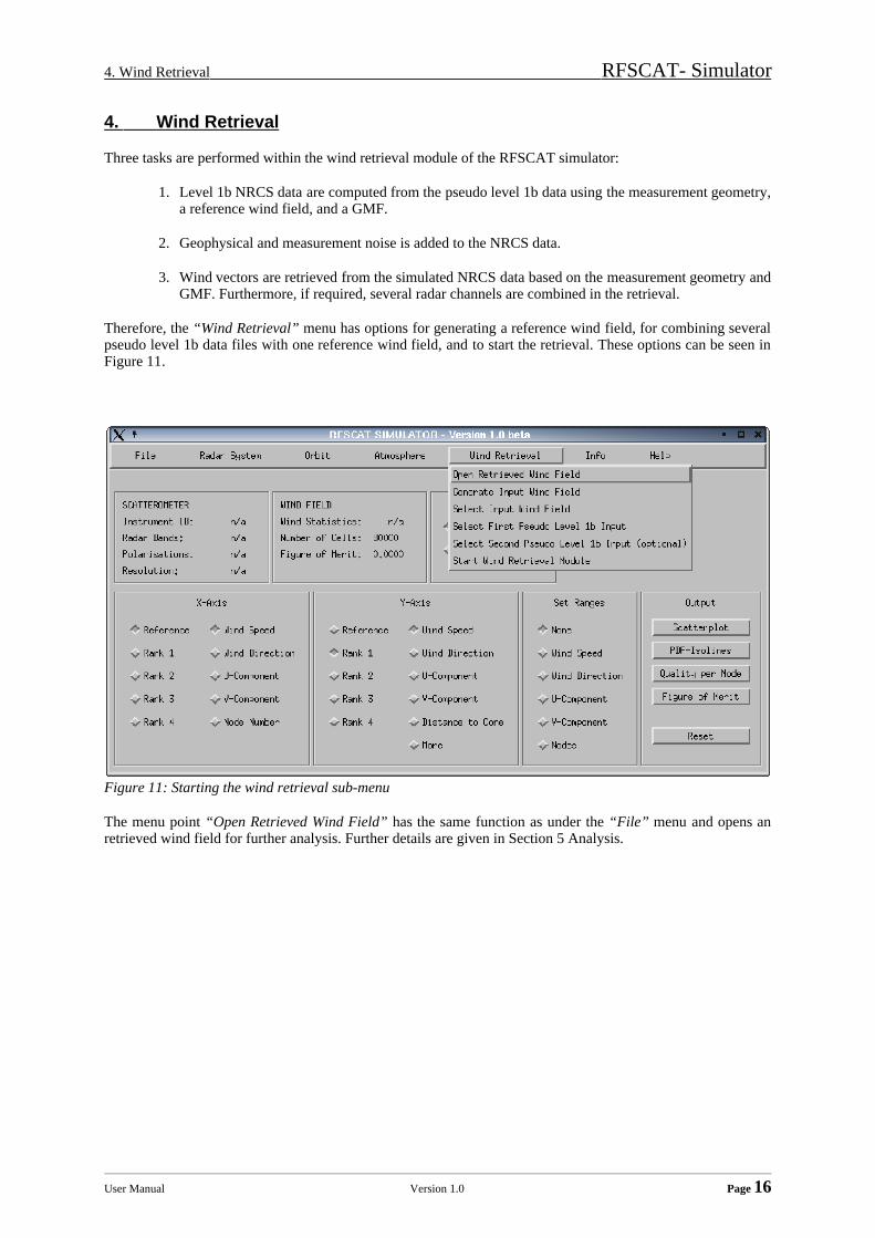
Three tasks are performed within the wind retrieval module of the RFSCAT simulator:

1. Level 1b NRCS data are computed from the pseudo level 1b data using the measurement geometry,a reference wind field, and a GMF.

2. Geophysical and measurement noise is added to the NRCS data.

3. Wind vectors are retrieved from the simulated NRCS data based on the measurement geometry andGMF. Furthermore, if required, several radar channels are combined in the retrieval.

Therefore, the “Wind Retrieval” menu has options for generating a reference wind field, for combining severalpseudo level 1b data files with one reference wind field, and to start the retrieval. These options can be seen inFigure 11.

Figure 11: Starting the wind retrieval sub-menu

The menu point “Open Retrieved Wind Field” has the same function as under the “File” menu and opens anretrieved wind field for further analysis. Further details are given in Section 5 Analysis.



4.1. Generating a Reference Wind Field

The menu point “Generate Input Wind Field” allows to create a reference wind field with a defined statistics.The u- and v-components of the wind field as well as the wind speed can be normally or uniformly distributedwith a given mean (only for normal distribution) and a given width. If a wind speed distribution is beingselected the wind direction is uniformly distributed. In the case of standard simulations of one orbit with 1500km or 1800 km swath width and resolutions of 50 km and 25 km the number of cells is set automatically.However, the number of wind vectors to be used in the retrieval can be set manually as well. The referencewind field will be stored under the given filename in the directory ../rfscat/wind (see Figure 12).


Figure 12: Defining the statistics of thereference wind field.


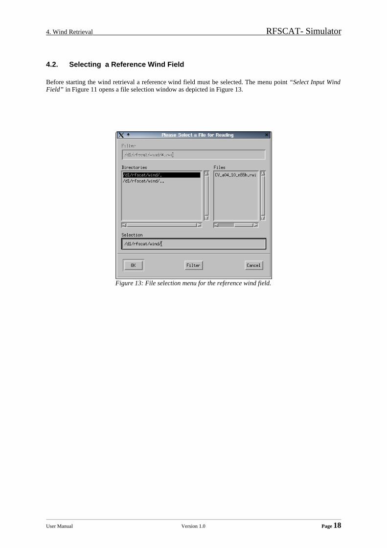
4.2. Selecting a Reference Wind Field

Before starting the wind retrieval a reference wind field must be selected. The menu point “Select Input WindField” in Figure 11 opens a file selection window as depicted in Figure 13.


Figure 13: File selection menu for the reference wind field.


4.3. Selecting Pseudo Level 1b Data

Before starting the wind retrieval at least one pseudo level 1b dataset must be selected. The menu point “SelectFirst Pseudo Level 1b Input” in Figure 11 opens a file selection window as depicted in Figure 14. Up to threeradar channels (pseudo level 1b datasets) can be combined in the current version of the RFSCAT simulator, viathe menu points “Select Second Pseudo Level 1b Input” and “Select Third Pseudo Level 1b Input”.


Figure 14: File selection menu for pseudo level 1b data.


4.4. Starting the Wind Retrieval

Before starting the wind retrieval via the menu point “Start Wind Retrieval Module” (see Figure 11) make surethat a reference wind field and at least one pseudo level 1b data file was selected, otherwise an error messagewill remind you.

The wind retrieval module is written in FORTRAN and called externally by the GUI. Consequently allmessages issued by this module will show-up in the terminal window from which IDL and the RFSCATsimulator were started and will not be displayed in pop-up windows like messages from the GUI.

The wind retrieval is a considerable computational effort, thus allow several minutes time for retrieving anentire orbit. The progress of the retrieval can be followed by the messages issued from the module in the mainIDL terminal window.

The resulting data will be stored in the respective .rwi file for further analysis (see Section 2.4 File Names fordetails).


5. Analysis RFSCAT- Simulator

5. Analysis

The third component of the RFSCAT simulator is the analysis tool. A retrieved wind field can be loaded via the“Open Retrieved Wind Field” menu point in the “File” menu (see Figure 15). This opens a file selection menuas depicted in Figure 16.

Figure 15: Main RFSCAT simulator window with the "File" menu.


Figure 16: File selection menu for the retrieved wind field.


5.1. Figure of Merit

Details on the Figure of Merit (FoM) concept are given in the Task-3a and Task-3b Reports. The FoM is ameasure of the quality of the wind retrieval. The output selection “Figure of Merit” starts a comprehensivecomputation of the retrieval performance as a function of node and finally of the FoM. The result displayed inthe WIND FIELD box of the main RFSCAT simulator window (see Figure 15).

5.2. Obtain the Quality Index

More detailed information is provided under the output-button “Quality per Node“ which also provides theFoM, but additionally displays the performance of the the RFSCAT system as a function of node across theinstrument swath as depicted in Figure 17. Herein the red line is the average performance and represents theFoM of this system.

The “PRINT” option creates a PostScript file of plot, while the “EXPORT” option creates an ASCII data filewith the values of quality index and node number. The code (see Figure 17) is generated on the basis of theactual date and time and used within the file name.


Figure 17: Display of the "Quality per Node".


5.3. Scatterplots

The analysis tool allows to plot the data is various ways. For comparing two datasets scatterplots are widelyused. Here the selection buttons on the main RFSCAT simulator window (see Figure 15) offer a wide range ofpossibilities for the X- and Y-axis.

The wind retrieval provides up to four solutions for the retrieved wind, which are ordered according to theirprobability from rank 1 to rank 4. Together with the reference wind field, five wind fields are at disposal fromwhich wind speed, wind direction, or one of the wind vector components u or v can be selected.

(a) (b)

(c) (d)

Figure 18: Examples for scatterplots.

Different examples of scatterplots are depicted in Figure 18. By default a linear regression is computed throughthe data points and the respective parameters are given in the display window. The regression line can beswitched on and off by the “Regression” button. Furthermore the data points can be connected by a line usingthe “Add Curve” button. This is recommended only when few data points are plotted like in Figure 18(d).

The “PRINT” option creates a PostScript plot of the scatterplot, while the “EXPORT” option creates an ASCIIdata file with the values pairs of the respective parameters. The code is generated on the basis of the actual dateand time and used within the file name.



5.4. PDF-Plots

Scatterplots might be difficult to survey when too many data points are plotted on top of each other. Here theirdensity distribution provides important information. Thus, all scatterplots can be displayed also as probabilitydensity functions (PDF) simply by toggling between the buttons “Scatterplot” and “PDF-Isolines” on the mainwindow of the RFSCAT simulator.

Figure 19 depicts examples of PDF-displays. The “PRINT” option creates a PostScript plot of the scatterplot,while the “EXPORT” option creates an ASCII data file with the values pairs of the respective parameters. Thecode is generated on the basis of the actual date and time and used within the file name.

(a) (b)

Figure 19: Examples of PDF plots.



5.5. Set Ranges

For a even more detailed analysis it might necessary to restrict the evaluation to certain ranges of wind speed,wind direction, wind components, or node numbers. The “Set Ranges” tool on the main RFSCAT simulatorwindow offers this possibility. The ranges can be selected individually in the respective “Adjust”-windows (seeFigure 20), either by editing the number directly or by using the scroll-bar with the mouse. The selection“None” will reset all parameters to their default values, which are +/- 25 m/s for the u- and v-component, 0.0-25.0 m/s for wind speed, 0-360 degrees for wind direction, and 0-72 for node number (corresponding to a 1800km wide swath and 25 km resolution).

Figure 20: "Adjust" windows for parameters.



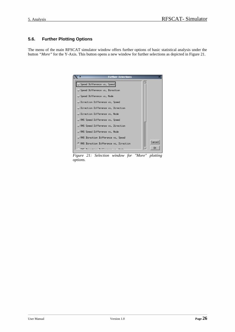
5.6. Further Plotting Options

The menu of the main RFSCAT simulator window offers further options of basic statistical analysis under thebutton “More” for the Y-Axis. This button opens a new window for further selections as depicted in Figure 21.


Figure 21: Selection window for "More" plottingoptions.


5.7. Changing the Reference System

The wind retrieval performance of a RFSCAT system might depend on the antenna azimuth angle with respectto the wind direction. Since the satellite heading varies considerably along one orbit this effect will not bevisible when plotting the results as a function of wind direction. Therefore, the coordinate system for the windvector can be switched between a geographical, which is the standard meteorological convention and a systemrelated the satellite heading, which varies accordingly along the orbit. The default setting is the geographicalsystem.


user manual for rfscat simulator -...

Documents

Transcript of user manual for rfscat simulator -...