U.S. DEPARTMENT OF THE INTERIOR

U.S. GEOLOGICAL SURVEY

EPOCH 2002 USERS' GUIDE FOR ULTRASONIC VELOCITY MEASUREMENTS IN GLACIER ICE

by

Joan J. FitzpatrickU.S.Geological Survey

Denver, CO

Open-File Report 92-534

This report is preliminary and has not been reviewed for conformity with U.S. Geological Survey editorial standards (or with the North American Stratigraphic Code). Any use of trade, product, or firm names is for descriptive purposes only and does not imply endorsement by the U.S. Government.

CONTENTS

Page

Abstract iii

Components of the EPOCH 2002......................................................................... 4Keypad layout............................... ......................................................................... .4

Operation..................... ....................................................................................................... 5Starting up and checking initial values................................................................ 5Calibrations............................................................................................................ 6

Delay or zero calibration........................................................................... 6Attenuation calibration..............................................................................?

Sample preparation.................................................................................. ............. .8Sample measurement................................................................................. ....... .....8

Troubleshooting................................................................................................................^

Selected bibliography......................................................................... ....... .................. .....11

FIGURES

Figure 1. Keypad layout for the Epoch 2002................................................................ 12

2. Full status display screen.............................................................................. 13

3. Example of full data screen for delay calibration.......................................14

4. Typical screen sequence during a measurement...................................15,16

5. Illustration of band saw cuts for vertical and transversep-wave measurements...................................................................................17

TABLES

Table 1. Manufacturer's specifications for the Epoch 2002......................................2,3

2. Information shown on the full status display only screen............................. 6

11

ABSTRACT

This report is an instruction manual in the set-up, calibration, and operation of the Panametrics Epoch 2002 ultrasonic testing workstation. Detailed procedures for sample preparation and measurement of differential p-wave velocities in fine-grained glacier ice are also outlined in this document. Measurement of the speed of propagation of elastic waves through ice in two mutually perpendicular directions, down and across the drilling axis of an ice core, yields information on the degree of orientation of ice crystals within the core and thus indicates the progress of fabric development as the ice recrystallizes in a stress field. Differential ultrasonic velocity measurements can be used both as a rapid screening method to track the progress of fabric development with increasing depth in an ice sheet or glacier and also to indicate zones of anomalous flow within the ice body. Additionally, measurement of both p- and s-wave velocities in a core allows computation of all elastic moduli.

in

INTRODUCTION

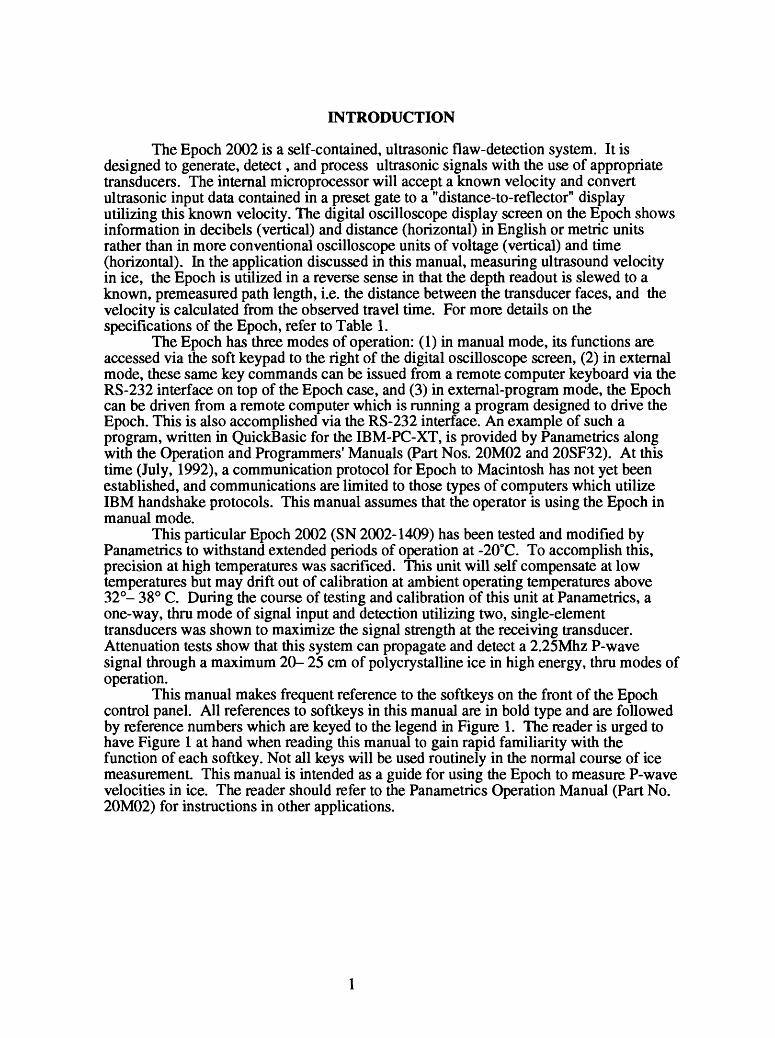
The Epoch 2002 is a self-contained, ultrasonic flaw-detection system. It is designed to generate, detect, and process ultrasonic signals with the use of appropriate transducers. The internal microprocessor will accept a known velocity and convert ultrasonic input data contained in a preset gate to a "distance-to-reflector" display utilizing this known velocity. The digital oscilloscope display screen on the Epoch shows information in decibels (vertical) and distance (horizontal) in English or metric units rather than in more conventional oscilloscope units of voltage (vertical) and time (horizontal). In the application discussed in this manual, measuring ultrasound velocity in ice, the Epoch is utilized in a reverse sense in that the depth readout is slewed to a known, premeasured path length, i.e. the distance between the transducer faces, and the velocity is calculated from the observed travel time. For more details on the specifications of the Epoch, refer to Table 1.

The Epoch has three modes of operation: (1) in manual mode, its functions are accessed via the soft keypad to the right of the digital oscilloscope screen, (2) in external mode, these same key commands can be issued from a remote computer keyboard via the RS-232 interface on top of the Epoch case, and (3) in external-program mode, the Epoch can be driven from a remote computer which is running a program designed to drive the Epoch. This is also accomplished via the RS-232 interface. An example of such a program, written in QuickBasic for the IBM-PC-XT, is provided by Panametrics along with the Operation and Programmers' Manuals (Part Nos. 20M02 and 20SF32). At this time (July, 1992), a communication protocol for Epoch to Macintosh has not yet been established, and communications are limited to those types of computers which utilize IBM handshake protocols. This manual assumes that the operator is using the Epoch in manual mode.

This particular Epoch 2002 (SN 2002-1409) has been tested and modified by Panametrics to withstand extended periods of operation at -20°C. To accomplish this, precision at high temperatures was sacrificed. This unit will self compensate at low temperatures but may drift out of calibration at ambient operating temperatures above 32°- 38° C. During the course of testing and calibration of this unit at Panametrics, a one-way, thru mode of signal input and detection utilizing two, single-element transducers was shown to maximize the signal strength at the receiving transducer. Attenuation tests show that this system can propagate and detect a 2.25Mhz P-wave signal through a maximum 20- 25 cm of polycrystalline ice in high energy, thru modes of operation.

This manual makes frequent reference to the softkeys on the front of the Epoch control panel. All references to softkeys in this manual are in bold type and are followed by reference numbers which are keyed to the legend in Figure 1. The reader is urged to have Figure 1 at hand when reading this manual to gain rapid familiarity with the function of each softkey. Not all keys will be used routinely in the normal course of ice measurement. This manual is intended as a guide for using the Epoch to measure P-wave velocities in ice. The reader should refer to the Panametrics Operation Manual (Part No. 20M02) for instructions in other applications.

Tab

le

1.

Man

ufac

ture

r's

Spec

ific

atio

n sh

eet

for

EP

OC

H 2

002.

Dis

pla

y

Gra

ticu

le

Sen

siti

vit

y

Rej

ect

Un

its

Vel

ocit

y

Zer

o O

ffse

t

Del

ay

Ran

ge

5" (

127)

dia

gona

lly m

easu

red

CR

T

Elec

troni

cally

gen

erat

ed 2

.25"

x 3

.125

" (5

7 x

80m

m) -

app

roxi

mat

e si

ze

HO

dB m

ax. r

eado

ut to

O.ld

B r

esol

utio

n w

ith a

utom

atic

refe

renc

e se

nsiti

vity

feat

ure

that

dis

play

s +

or -

devi

atio

n fr

om

refe

renc

e se

nsiti

vity

.

Abs

olut

ely

linea

r to

70%

of f

ull s

cale

.

Eng

lish

or m

etric

by

rear

pan

el s

witc

h se

lect

ion.

0.02

5 to

0.6

in /

jis

(635

tol

5240

m/s

)

0 to

200

|LIS

(Allo

ws

com

pens

atio

n fo

r ac

oust

ic s

ound

pat

h tim

e in

wed

ges

and

dela

y lin

es in

ord

er to

cal

cula

te s

ound

pa

th a

nd d

epth

.)

Fixe

d de

lays

of 0

, 1,

2, 5

, 10

, 20,

50,

100

, 20

0 in

. or

0,

10, 2

0, 5

0, 1

00,

200,

500

, 10

00,

2000

, 500

0mm

or

vari

able

fro

m 0

to 3

50 in

. 0

to 8

900m

m a

t the

vel

ocity

of l

ongi

tudi

nal

Pea

k M

emor

y

Ave

M

emor

y

Loc

k

Tes

t M

odes

Dis

play

U

pdat

e R

ate

Dig

itiz

atio

n

Rat

e

Ala

rms

wav

es in

ste

el.

Key

boar

d A

nnun

ciat

or

Exp

ansi

on

Fixe

d ra

nges

of

0.1,

0.2

, 0.

5, 1

.0, 2

.0,

5.0

in./

div.

or

2, 5

, 10

, 12

.5,

20,

25,

50,

100

mm

/div

or v

aria

ble

from

0.0

6 to

7.4

in./d

iv.

or 1

.5 t

o 19

0mm

/div

. at t

he v

eloc

ity o

f lo

ngitu

dina

l wav

es in

ste

el;

0.3

to 4

.0 in

./div

. or

.76

to 1

02m

m/d

iv a

t the

vel

ocity

of s

hear

w

aves

in s

teel

. O

ptio

nal e

xten

ded

rang

e is

av

aila

ble.

Aut

omat

ical

ly e

xpan

ds g

ated

por

tion

of

disp

lay

to fu

ll gr

atic

ule

wid

th.

Ou

tpu

ts

Siz

e

Prod

uces

sto

red

disp

lay

repr

esen

ting

max

imum

si

gnal

at a

ll lo

catio

ns.

(Use

d fo

r st

orin

g ec

hody

nam

ic.)

Prod

uces

sto

red

disp

lay

repr

esen

ting

the

aver

age

ampl

itude

at a

ll lo

catio

ns f

or u

p to

102

4 di

spla

y up

date

s.

Ena

bles

mos

t sys

tem

fun

ctio

ns to

be

lock

ed a

t pr

eset

val

ue to

avo

id a

ccid

enta

l rea

djus

tmen

t.

Puls

e-ec

ho o

r thr

ough

tran

smis

sion

(pi

tch

and

catc

h).

60H

z at

test

freq

uenc

ies

low

er th

an 4

MH

z.

25H

z or

gre

ater

at 4

- 6

MH

z, a

nd b

road

band

fi

lter

posi

tions

.

20-4

0MH

z at

test

freq

uenc

ies

low

er th

an 4

MH

z.

65-8

0MH

z at

4-6

MH

z, 1

0MH

z, a

nd b

road

band

fi

lter

posi

tions

.)

Vis

ual o

n di

spla

y sh

owin

g m

axim

um a

nd c

urre

nt

valu

e of

def

ect s

igna

l am

plitu

de in

gat

e. A

udib

le

horn

or e

arph

one.

Rea

r pan

el s

witc

h co

ntro

ls a

udib

le to

ne w

hen

key­

pa

ds a

re d

epre

ssed

.

Ana

log

outp

ut 0

to 1

vol

t pro

port

iona

l to

sign

al

ampl

itude

in g

ate.

Com

posi

te v

ideo

out

put,

75 o

hms

outp

ut im

­ pe

danc

e, 1

vol

t sig

nal l

evel

into

75

ohm

s, b

lack

ne

gativ

e, s

ync

nega

tive.

(A

llow

s in

terf

ace

with

a

vide

o pr

inte

r, V

CR

or v

ideo

mon

itor.)

10.2

5 x

4.75

x 1

2 in

ches

26

0 x

121

x 30

5 m

m

Tab

le 1

. M

anuf

actu

rer'

s Sp

ecif

icat

ion

shee

t fo

r E

PO

CH

200

2 (c

onti

nued

)

Dis

tanc

e R

eado

ut

Ref

ract

ed

Ang

le

Gat

e St

art

Gat

e W

idth

Gat

e L

evel

Tim

e V

arie

d G

ain

Dam

pin

g

Rec

tifi

er

Fre

quen

cy

Ran

ge

Pu

lser

Stat

us

Rea

dout

Prov

ides

sou

nd p

ath,

sur

face

, and

dep

th to

0.

001

in. o

r 0.0

4mm

reso

lutio

n

Can

be

ente

red

at 0

.0°

or 1

0 to

85°

re

frac

ted

angl

e in

0.1

° an

gle

reso

lutio

n.

Var

iabl

e ov

er c

ompl

ete

disp

lay

rang

e w

ith

loca

tion

read

out i

n un

its o

f met

al p

ath.

Var

iabl

e ov

er d

ispl

ayed

rang

e w

ith re

adou

t in

uni

ts o

f met

al p

ath.

Off

or o

n w

ith le

vel a

djus

tabl

e fr

om 4

to

80%

of f

iill s

cree

n.

Dis

tanc

e am

plitu

de c

orre

ctio

n w

ith re

solu

­ tio

n be

twee

n co

rrec

tion

poin

ts o

f 2(j.

s min

. an

d 30

dB d

ynam

ic ra

nge.

Gai

n cu

rve

can

be

of ar

bitra

ry s

hape

. Li

near

inte

rpol

atio

n is

m

ade

betw

een

corr

ectio

n po

ints

.

Fixe

d se

tting

s of

60,

80,

150

, and

400

ohm

s

Full

wav

e, h

alfw

ave

posi

tive

and

nega

tive

Bro

adba

nd (-

6dB

): 0.

5 to

15

MH

z N

arro

wba

nd (I

dB f

latn

ess)

: 0.4

- 0.

6,

0.9-

1.1,

2-4

,4-6

, 9-

11 M

Hz

Shoc

k ex

cita

tion,

-40

0V, o

pen

circ

uit,

high

and

low

ene

rgy

Wei

ght

12.5

Ibs

. (5.

7 K

g) w

ithou

t bat

tery

17

Ibs.

(7.7

Kg)

with

bat

tery

pac

k

Ope

rati

ng

Tem

pera

ture

-2

0°C

(+2

5°C

typi

cal)

to 5

0°C

Stor

age

Tem

pera

ture

-4

0°to

60°C

Bat

tery

Pac

k Q

uick

dis

conn

ect b

atte

ry p

ack

allo

ws b

atte

ry

pack

to b

e ch

arge

d w

ithou

t ope

ning

uni

t.

Bat

tery

T

ype

12 v

olt s

eale

d le

ad-le

ad d

ioxi

de b

atte

ry

Bat

tery

L

ife

12 h

rs. @

25°

C

Bat

tery

St

atus

Fu

ll sc

reen

bat

tery

sta

tus

indi

cato

r via

fron

t pa

nel k

eypa

d sh

ows

stat

e of

char

ge.

Bat

tery

Cha

rger

Sh

ort c

ircui

t pro

of b

atte

ry c

harg

er c

apab

le o

fop

erat

ing

unit

and

char

ging

bat

tery

sim

ulta

neou

sly

AC

R

equi

rem

ents

82

to 1

30 V

AC

/164

to 2

60 V

AC

, 47

to 6

6 H

z.

30 w

att m

axim

um.

Cha

rgin

g T

ime

16 h

ours

max

. dep

endi

ng o

n st

ate

of ch

arge

Pow

er

Con

sum

ptio

n 6

wat

ts

Tra

nsdu

cer

Con

nect

or

BN

C o

r Num

ber

1 L

emo

Han

dle/

Tilt

St

and

Var

iabl

e po

sitio

n, lo

ckin

g ty

pe

Dis

play

s lis

t of a

ll sy

stem

fun

ctio

ns w

ith

pres

ent v

alue

of e

ach

func

tion.

Abi

lity

to

supe

rimpo

se th

e st

atus

dis

play

ove

r the

A-s

can

for d

ocum

enta

tion.

10

Stor

ed

Abi

lity

to s

tore

, rec

all a

nd c

lear

10

dist

inct

M

emor

y Se

t-up

tra

nsdu

cer c

alib

ratio

ns

Components of the Epoch

The Epoch is a compact, field-portable unit which includes several subsystems. These subsystems are the digital oscilloscope and its attendant controls (gain and reject, distance and time base, peak and average memory), the pulser/receiver controls for the generation and detection of the ultrasonic signals (frequency filtering, pulse energy, signal damping), the internal microprocessor controls (gate controls, status and memory, recall and store setup functions, status and lock), and the transducers. The performance of the system, as a whole, depends on the optimization of the performance of the individual subsystems for the particular analytical task at hand. The settings which are recommended in this manual have proven to yield good results on fine-grained glacier ice. The settings recommended here may not yield the best possible results on other types of materials.

Keypad Layout

Figure 1 shows the layout of the softkey pad on the front of the Epoch. The keys are color coded into groups according to their function. The keys are grouped as follows:

Color Key Nos. Functions

Blue 1,7,3 gain and reject (vertical display axis)

Yellow 2,3,8,9,10,14,15 distance and time base (horizontal displayaxis)

Red 4,5,6 gate adjustment

Brown 11,12,17,18,23 pulser/receiver controls

Orange 16,20,21,22 status and memory/

Additional special keys include the two large green slewing keys [19 and 24], the yellow battery level key [25], and the green power key [26].

OPERATION

Starting Up and Checking Initial Values

Before using the Epoch, an initial check of starting settings should be made. These include the following:

Rear Panel Settings:audio alarm - off

units - mm composite video - connected to printer or an auxiliary screen

The Epoch can be run either on battery power or AC-line power (115 or 230V). To run on battery power, seat the battery pack firmly on the two guide pins provided on the back panel of the Epoch, making sure that the 4-pin receptacle on the battery pack is aligned with the 4-pin plug on the Epoch. Tighten the thumbscrews on either side of the seating pins. The battery level may be examined any time the Epoch is running by pressing the battery level key [25]. If the battery power runs low during the course of operation, the Epoch can continue to operate while recharging the battery by connecting the charger/adapter into the battery back at the 4-pin connector on the side of the battery pack. To run on AC-line power, select the appropriate line voltage by means of the slide switch on the back of the charger/adapter, connect the charger/adapter to the Epoch by means of the 4-pin connector on the end of the DC output cable, connect the charger/adapter power cable to the line power source, and turn it on by means of the power switch on the front. To power up the Epoch, press the green power key [#26] on the front panel. If the Epoch is operating properly, it will beep as the power comes on, and the Panametrics logo will appear on the screen within five seconds. The unit will self-test for approximately ten seconds. When the self-test is competed the unit is ready for operation. Press the orange status display key [#16] until the full status screen is displayed (Figure 2). Values on the status display screen should appear as shown in Table 2.

Adjust the parameters on the screen to match those shown in Table 2 by one of two methods. The user may recall the correct stored setup from memory by entering the status only display mode (depressing key #16 twice), selecting memory position #1 with the right slew key [19], and pressing the average memory key [22]. Readjustment of the values for parameters shown on the status display screen may also be accomplished by resetting the values of the chosen parameter using the keys indicated at the left and right of each status line listed in Table 2. For example, if the frequency key [18] is pressed several times, the value shown under the parameter labeled "FILTER" on the status display screen will scroll through the values 0.5, 1.0, 2 to 4, 4 to 6, 10, and BROADBAND. If the mode key [23] is pressed, the value will toggle from thru mode to T/R mode (transmit and receive). The reject [1], delay [14], and zero [8] keys are designed to slew through a continuum of values rather than scroll through a table of preset values. To reset any of these values, first press the desired function key and then slew to higher or lower values, using one of the two slew keys [19 and 24].

Table 2. Information shown on the full status display only screen

KEY# KEY#

1 REJ 0% xxxx* mm/DIV 15

13 xxxx dB

14 DELAY xxxx mm ZERO 2.43 us 8

18 FILTER broadband DAMPING 400 OHMS 11

4 GATE START xxxx ENERGY HIGH 17

5 GATE WIDTH xxxx HALFWAVE+ 12

6 GATE LEVEL 60% THRU MODE 23

2 VELxxxxM/sec < 0.0° / 0.00 mm 3

* values which are not critical at startup are indicated as xxxx

Calibrations

Delay or Zero Calibration

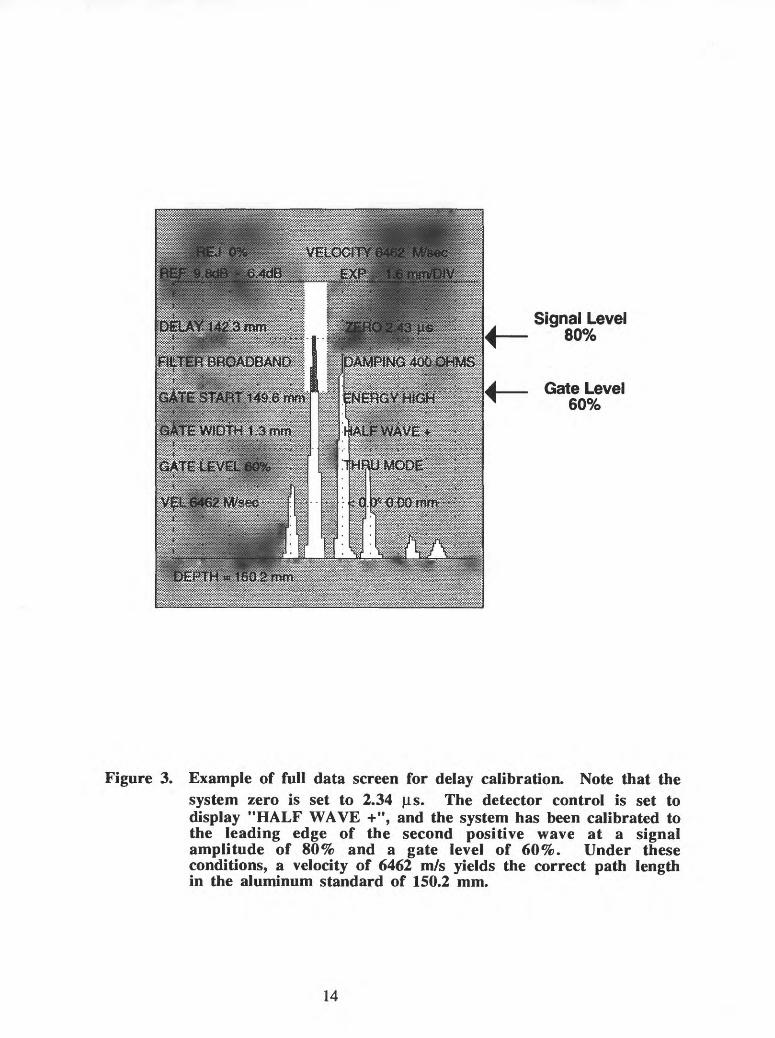
The first procedure necessary to acquire data is the determination of the travel time required for the ultrasonic signal to pass through everything exclusive of the sample itself. This includes the cables, backing plates, transducers, wearplates, and any buffer rods. This calibration should be made in two circumstances: (1) when the configuration of the system is changed, i.e. if a transducer or cable is changed, if a buffer rod is introduced, or if anything is done which changes the sound path length (exclusive of path length in the sample itself), or (2) when the operator chooses to change the portion of the signal over which the gate will be set for measurement, i.e. the operator wishes to redefine the first arrival in the wave train. An aluminum rod with a length-velocity- temperature calibration curve has been provided for this purpose. The factory calibrateddelay (or "zero") for the system as it is configured for ice measurements is 2.43 (is. Due to the internal quartz crystal time-base compensation of the unit, the delay or system zero is temperature insensitive. Although the operator should periodically check the delay calibration, the value of the system zero should not change during the course of normaloperation. The value of 2.43 (is assumes that the operator is using the two 6' HDAS cables, the 2.25Mhz transducers labeled 1 and 2, that glycerine bonding solution (Couplant B) is used to couple the transducers to the sample, that no buffer rods are used, and that the chosen first arrival is the leading edge of the second positive wave front (in the half-wave positive display) at a maximized peak signal of 80 percent and a gate level of 60 percent (see Figure 3). This is the standard configuration in which all measurements are made. If the operator chooses to change this configuration or to redefine the first arrival, the system zero must be recalibrated. The travel time in the

Epoch 2002 is calculated from the main bang to the first signal crossing into the gate minus the zero offset. Note that, using this algorithm, consistent setting of the signal peak and gate levels is crucial.

To check the calibration or redefine the system zero, ascertain that the ends of the aluminum rod are free from any buildup of ice or frost and then measure the length of the aluminum rod with a micrometer. This measurement should be precise to the nearest 0.1 mm. Measure the temperature of the rod and check these values against the calibration curve provided. Read the correct velocity off the curve or compute it from the equation provided. Ascertain that the Epoch is in thru-transmission mode, not transmit/receive mode using the status key [16], and that the detector control key [12] is in half-wave positive mode. Verify that the zero delay is set to 2.43 microseconds from the status display. Connect transducers #1 and #2 to the two HDAS cables and connect the cables to the Epoch. Apply three to four drops of warm glycerine to the center of the upturned face of one of the transducers, set it on a flat surface, and place the aluminum rod upright on the face of this transducer. Move the rod over the transducer with a circular motion until it wrings in slightly. Apply three to four more drops of glycerine to the center of the upright face of the aluminum rod and wring in the second transducer. At this point, a signal should be visible on the oscilloscope screen. If it is not, shrink the horizontal scale using the range key [15] until the signal is located, drag the gate over the signal using the gate position key [4], and then expand the screen using the range expansion key [9]. The gate and signal will now appear at the far left edge of the oscilloscope screen. To drag it to the center of the screen, press the delay key [14] once and use the slew keys [19 and 24] to reposition the signal and gate in the center of the screen. Adjust the position of the upper transducer on the face of the aluminum rod until the strongest signal possible is achieved. Leaving the transducers in the same position relative to each other, increase the signal to 80 percent by pressing the dB key [13] once and the up slew key [19]. Reposition the gate over the signal if necessary and drop the gate level to 60 percent using the gate position [4], gate level [6], and slewing keys [19 and 24]. Press the sound velocity key [2], slew the displayed value to the correct sound velocity of the calibration rod from the calibration curve and then press the distance to reflector key [3]. The depth displayed on the lower left corner of the screen should match the measured half length of the aluminum rod. If you have changed the system configuration or wish to redefine the portion of the wave train you are measuring, use the zero offset [8] and slew keys [19 and 24] to adjust the system zero value until the correct path length is displayed for the calibrated velocity.

Attenuation Calibration

If the operator intends to measure relative acoustic attenuation as well as velocity, the system must be standardized to a stable reference material. Measurement of the signal attenuation in this standard provides a constant point of comparison for measurements of attenuation in ice samples. (Absolute acoustic attenuation cannot be measured with this system.) A small leucite block with two polished ends has been provided for this purpose. The loss characteristics of this block are such that a 10 cm truepath in ice will generally result in a positive signal loss relative to the standard (i.e. more signal is lost in the ice than in the standard). To perform this calibration, measure the signal as described in the delay calibration section, omitting the path-length measurement step. When coupling the transducers onto the block, visually inspect the bond through the leucite and confirm that the entire face of the transducer is bonded to the standard block. Position the transducers to maximize the signal and increase the gain

until the signal reaches the 80 percent level. Drag the gate over the signal, set the gate level to 60 percent, and then depress the reference level key [7] twice. The new reference level should now appear in the upper left hand corner of the live screen. Do not press the reference level key again after the measurement has been made because this will cause the reference level to be reset to whatever level happens to be present in the gate at the time. After this calibration is completed, all other attenuation measurements will appear appended to this reference level as + or - values in decibels following the calibrated reference level. A positive value indicates that the measured sample has a larger acoustic loss than the reference standard and a negative value indicates that the sample has a smaller loss value.

Sample Preparation

Core samples should be trimmed with a band saw so that opposite pairs of faces are plane parallel to each other. Lack of plane-parallelism in these cuts is the major source of error in the velocity measurements. If no azimuth control is available on the core, two perpendicular sets of faces for the determination of longitudinal and transverse velocity are sufficient. If azimuth control is available, one set of faces for the longitudinal velocity and two perpendicular sets of faces for the transverse velocities should be cut. Cuts for the transverse velocity measurements should be made parallel and perpendicular to the direction of flow (see Figure 5). After the cuts are made, the cut faces should be sanded to smoothness on a wire mesh-covered, flat surface. Sanding should remove all traces of saw cuts and loose chips of ice . The distances between parallel faces can then be measured by calipers. These measurements should be repeated several times and averaged to obtain an estimate of the anticipated error arising from the uncertainty in the measurement of the path length.

Sample Measurement

Couple the transducers onto the ice sample with a small amount of warm couplant using a gentle wringing motion. Visually inspect the bond through the ice and confirm that the entire face of each transducer is bonded. If normal-incidence s-wave transducers are being used, apply several drops of cold water to the face of the transducer and freeze it onto the sample instead. Bring up the live waveform display on the Epoch using the status key [16]. If no signal appears on the screen, check the gain [13]. For a path length of approximately 10 cm of ice, the gain should be approximately +35dB relative to the standard. If the signal is not yet visible, either scroll along the screen using the delay key [14] or compress the horizontal axis using the range key [15] until the signal is located. When the signal is located, drag the gate [4] so that it is positioned over the second peak and adjust the gain again [13] to bring the signal above the gate level. Expand the range [9], if needed, so that the first arriving wave train fills the screen (Figure 4). Re-center the wave train on the screen if necessary. Position the transducers so that the amplitude of the signal is maximized. Investigate the sound paths through the sample by moving the transducers over the ice and watching the arrival time change. If large cracks are present in the sample or if the grain size is on the order of magnitude of the transducer diameter, large shifts in the velocity may be observed. Such samples may be unsuitable for analysis. Samples of deep ice that contain high concentrations of exsolved hydrate clathrates can also exhibit strong attenuation characteristics in directions normal to the exsolution plane. Anomalously low velocities will also be observed in these directions

because the truepath length may be longer than the measured distance between the transducers.

When the position of the transducers yields a satisfactory signal, readjust the gain [13] so that the peak amplitude of the second wave (in half-wave positive mode) is 80 percent of the full vertical scale. Reposition the gate, if necessary, so that the leading edge of this portion of the wave train crosses into the gate at a level of 60 percent [6]. Press the distance to reflector key [3] to bring up the depth display in the lower left corner of the screen and press the sound velocity key [2] to bring up the velocity display in the upper right corner. Adjust the velocity until the correct value for the half-path length appears in the depth window. The velocity displayed in the upper right corner is now the correct velocity for the measured depth. To save the screen and status information for printing, press the status key [16] until the full status screen and the live data screen are superimposed. Press the average memory key [22] to freeze the screen and print the screen contents using the video printer chained to the Epoch. Repeat this process for the transverse measurements.

Record the temperature of the sample at the time of measurement. The measured velocities can be corrected back to the in-situ temperature using the data tabulated in Kohnen (1974) where it is shown that

dVp /dT = -2.3m/sper°C dVs /dT = -1.2m/sper°C

Poisson's ratio and the pertinent elastic moduli can be calculated using the corrected data plus the temperature corrected densities.

TROUBLESHOOTING

No signal visible. Ascertain that the Epoch is functioning properly by decreasing the delay to 0.0 [Key 14] and increasing the gain [13] until the main bang is visible on the left edge of the screen. If no signal is visible, check the bnc connections between the cables and the Epoch and between the cables and the transducers. If the Epoch is functioning properly and the main bang is visible, slew the delay [14] to scroll across the screen without resetting the gain. If the signal is still not visible, check the filter [18] and damping controls [11] and the coupling at the transducers.

Noisv signal. Occasionally, samples with very high attenuation will yield very weak wave trains. If the sample cannot be cut thinner to allow more of the signal through, use the linear reject key [1] and average memory key [22] to improve the signal-to-noise ratio. Decoupling one of the transducers will help distinguish between what is signal and what is noise at very high gain settings. Very poor peak-to-background characteristics may be an indication that the sample is highly microcracked or is otherwise discontinuous (as in firn). Changing to a larger transducer may be helpful.

Inconsistent Signal. Remeasurement of a sample may yield inconsistent velocities if sound paths of varying lengths exist within the sample. It is advisable to investigate the propagation characteristics of the sample at the time of measurement by moving the transducers over the sample to insure that the measured velocity is the fastest the sample will yield. If possible, it is also advisable to make several measurements on an individual sample cut to successively shorter and shorter path lengths. If the velocity remains constant throughout this process, it may be assumed that the path length measured by calipers accurately reflects the truepath of the ultrasound waves through the ice.

10

SELECTED BIBLIOGRAPHY

Bennett, H.F., 1972, Measurements of ultrasonic wave velocities in ice cores from Greenland and Antarctica: U.S. Army Cold Regions Research and Engineering Laboratory Research Report 237, Hanover, NH, 58 p.

Bentley, C.R., 1972, Seismic-wave velocities in anisotropic ice: A comparison ofmeasured and calculated values in and around the deep drill hole at Byrd Station, Antarctica, Journal of Geophysical Research, v. 77, p. 4406-4420.

Gow, A.J. and Kohnen, H., 1978, Ultrasonic measurements on deep ice cores from Antarctica: Antarctic Journal of the United States, p. 48-50.

Gow, A.J. and Kohnen, H., 1979, The relationship of ultrasonic velocities to c-axis fabrics and relaxation characteristics of ice cores from Byrd Station, Antarctica: Journal of Glaciology, v. 24, p. 147-154.

Herron, S.L., Langway, C.C., Jr., and Brugger, K.A., 1985, Ultrasonic velocities and crystalline anisotropy in the ice core from Dye 3, Greenland, in Langway, C.C., Jr., Oeschger, H., and Dansgaard, W., eds., Greenland Ice Core: Geophysics, Geochemistry, and the Environment: American Geophysical Union Monograph 33, p. 23-31.

Kohnen, H., 1974, The temperature dependence of seismic waves in ice: Journal of Glaciology, v. 13, p. 144-147.

Kohnen, H. and Gow, A.J., 1979, Ultrasonic velocity investigations of crystal anisotropy in deep ice cores from Antarctica: Journal of Geophysical Research, v. 84, p. 4865-4874.

Krautkramer, J., and Krautkramer, H., 1990, Ultrasonic Testing of Materials, Springer- Verlag, Berlin., 423 p.

Pao, Y.H., ed., 1978, Elastic Waves and Non-Destructive Testing of Materials: American Society of Mechanical Engineers, Applied Mechanics Division Symposia Series, v. 29, 143 p.

11

1

7

13

2

8

14

19

24

3

9

15

20

25

4

10

16

21

26

5

11

17

22

6

12

18

23

i£OdB-l-

-A.

dB

tyisece y * 0 *

^ A __ ̂

IK-4-4< j

JjAU

iQQri'fc

^=~L

M?

PEAK MEM

'V

j-t

c a rl

TAVE MEM

FEE! PANAMETRICSE

A

jnnk

MHz

5

:POCH2002

1. REJECT (LINEAR)

2. SOUND VELOCITY / REFRACTED ANGLE

3. DISTANCE TO REFLECTOR

4. GATE POSITION

5. GATE WIDTH

6. GATE LEVEL

7. REFERENCE LEVEL

8. ZERO OFFSET

9. RANGE EXPANSION

10. TIME VARIED GAIN

11. DAMPING

12. DETECTOR CONTROL

13. SENSITIVITY (GAIN)

14. DELAY

15. RANGE

16. STATUS

17. ENERGY

18. FREQUENCY (FILTER)

19. SLEW (UP, RIGHT)

20. KEYBOARD LOCK

21. PEAK MEMORY

22. AVERAGE MEMORY

23. MODE

24. SLEW (DOWN, LEFT)

25. BATTERY STATUS

26. POWER (ON/OFF)

Figure 1. Keypad layout for the Epoch 20002

12

Figure 2. Full status display screen. After initial power up, press the status softkey twice to obtain this screen,

13

Signal Level 80%

Gate Level60%

Figure 3. Example of full data screen for delay calibration. Note that the system zero is set to 2.34 [is. The detector control is set to display "HALF WAVE +", and the system has been calibrated to the leading edge of the second positive wave at a signal amplitude of 80% and a gate level of 60%. Under these conditions, a velocity of 6462 m/s yields the correct path length in the aluminum standard of 150.2 mm.

14

Fig.

4A

Fig.

4B

Figu

re 4

. T

ypic

al s

cree

n se

quen

ce d

urin

g a

mea

sure

men

t.

A

Sign

al a

s it

app

ears

in

com

pres

sed

disp

lay.

H

ere

the

gate

lie

s ju

st t

o th

e le

ft o

f th

e si

gnal

.

B.

Sam

e sc

reen

aft

er t

he g

ate

is r

epos

ition

ed o

ver

the

peak

.

Figu

re 4

CFi

gure

4D

Figu

re 4

. (c

ont.)

C

Sam

e sc

reen

aft

er r

ange

exp

ansi

on k

ey (

9) i

s ac

tiva

ted.

band-saw cuts drilling direction20cm

maximumlength

5b. Illustration of band saw cuts for vertical p-wave measurements.

flow direction and normals

core cross section

5b. Illustration of band saw cuts for transverse p-wave measurements with azimuth control.

Figure 5. Illustration of band saw cuts for vertical and transverse p-wave velocity measurements.

17