
URBAN CLASSIFICATION WITH SENTINEL-1 Case …...URBAN CLASSIFICATION WITH SENTINEL-1 Case Study:...
27
_p URBAN CLASSIFICATION WITH SENTINEL-1 Case Study: Germany, 2018 TRAINING KIT – LAND06 DFSDFGAGRIAGRAGRI
Transcript of URBAN CLASSIFICATION WITH SENTINEL-1 Case …...URBAN CLASSIFICATION WITH SENTINEL-1 Case Study:...

_p
URBAN CLASSIFICATION WITH SENTINEL-1 Case Study: Germany, 2018
TRAINING KIT – LAND06 DFSDFGAGRIAGRAGRI

2
Research and User Support for Sentinel Core Products
The RUS Service is funded by the European Commission, managed by the European Space
Agency and operated by CSSI and its partners.
Authors would be glad to receive your feedback or suggestions and to know how this
material was used. Please, contact us on [email protected]
Cover images produced by RUS Copernicus
The following training material has been prepared by Serco Italia S.p.A. within the RUS
Copernicus project.
Date of publication: October 2018
Version: 1.2
Suggested citation:
Serco Italia SPA (2018). Urban Classification with Sentinel-1 – Case Study: Germany 2018
(version 1.2). Retrieved from RUS Lectures at https://rus-copernicus.eu/portal/the-rus-
library/learn-by-yourself/
This work is licensed under a Creative Commons Attribution-NonCommercial-ShareAlike 4.0
International License.
DISCLAIMER While every effort has been made to ensure the accuracy of the information contained in this publication, RUS Copernicus does not warrant its accuracy or will, regardless of its or their negligence, assume liability for any foreseeable or unforeseeable use made of this publication. Consequently, such use is at the recipient’s own risk on the basis that any use by the recipient constitutes agreement to the terms of this disclaimer. The information contained in this publication does not purport to constitute professional advice.

3
Table of Contents
1 Introduction to RUS ......................................................................................................................... 4
2 Urban mapping – background ......................................................................................................... 4
3 Training ............................................................................................................................................ 4
3.1 Data used ................................................................................................................................. 4
3.2 Software in RUS environment ................................................................................................. 4
4 Register to RUS Copernicus ............................................................................................................. 5
5 Request a RUS Copernicus Virtual Machine .................................................................................... 6
6 Step by step ................................................................................................................................... 10
6.1 Data download – ESA SciHUB ................................................................................................ 10
6.2 Download data ...................................................................................................................... 10
6.3 Sentinel-1 SNAP Preprocessing ............................................................................................. 13
6.3.1 Read ............................................................................................................................... 14
6.3.2 TOPSAR-Split .................................................................................................................. 14
6.3.3 Apply Orbit File .............................................................................................................. 15
6.3.4 Back Geocoding ............................................................................................................. 15
6.3.5 Enhanced Spectral Diversity .......................................................................................... 16
6.3.6 Coherence...................................................................................................................... 16
6.3.7 TOPSAR Deburst ............................................................................................................ 17
6.3.8 Multi-look ...................................................................................................................... 17
6.3.9 Terrain correction .......................................................................................................... 18
6.3.10 Subset ............................................................................................................................ 19
6.3.11 Write .............................................................................................................................. 19
6.4 Import vector data ................................................................................................................ 20
6.5 Random Forest Classification ................................................................................................ 20
7 Extra Steps ..................................................................................................................................... 23
7.1 Coherence images ................................................................................................................. 23
7.2 Create Stack ........................................................................................................................... 24
7.3 Multi-temporal Random Forest classification ....................................................................... 26
8 Further reading and resources ...................................................................................................... 27
4
1 Introduction to RUS
The Research and User Support for Sentinel core products (RUS) service provides a free and open
scalable platform in a powerful computing environment, hosting a suite of open source toolboxes
pre-installed on virtual machines, to handle and process data derived from the Copernicus Sentinel
satellites constellation.
In this tutorial, we will employ RUS to run a supervised classification using the Random Forest
algorithm and Sentinel-1 SLC data as input data over an area in Bochum, Germany.
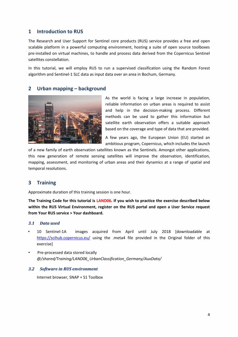
2 Urban mapping – background
As the world is facing a large increase in population,
reliable information on urban areas is required to assist
and help in the decision-making process. Different
methods can be used to gather this information but
satellite earth observation offers a suitable approach
based on the coverage and type of data that are provided.
A few years ago, the European Union (EU) started an
ambitious program, Copernicus, which includes the launch
of a new family of earth observation satellites known as the Sentinels. Amongst other applications,
this new generation of remote sensing satellites will improve the observation, identification,
mapping, assessment, and monitoring of urban areas and their dynamics at a range of spatial and
temporal resolutions.
3 Training
Approximate duration of this training session is one hour.
The Training Code for this tutorial is LAND06. If you wish to practice the exercise described below
within the RUS Virtual Environment, register on the RUS portal and open a User Service request
from Your RUS service > Your dashboard.
3.1 Data used
• 10 Sentinel-1A images acquired from April until July 2018 [downloadable at
https://scihub.copernicus.eu/ using the .meta4 file provided in the Original folder of this
exercise]
• Pre-processed data stored locally
@/shared/Training/LAND06_UrbanClassification_Germany/AuxData/
3.2 Software in RUS environment
Internet browser, SNAP + S1 Toolbox

5
4 Register to RUS Copernicus
To repeat the exercise using a RUS Copernicus Virtual Machine (VM), you will first have to register as
a RUS user. For that, go to the RUS Copernicus website (www.rus-copernicus.eu) and click on
Login/Register in the upper right corner.
Select the option Create my Copernicus SSO account and then fill in ALL the fields on the Copernicus
Users’ Single Sign On Registration. Click Register.
Within a few minutes you will receive an e-mail with activation link. Follow the instructions in the e-
mail to activate your account.
You can now return to https://rus-copernicus.eu/, click on Login/Register, choose Login and enter
your chosen credentials.

6
Upon your first login you will need to enter some details. You must fill all the fields.
5 Request a RUS Copernicus Virtual Machine
Once you are registered as a RUS user, you can request a RUS Virtual Machine to repeat this exercise
or work on your own projects using Copernicus data. For that, log in and click on Your RUS Service →
Your Dashboard.

7
Click on Request a new User Service to request your RUS Virtual Machine. Complete the form so that
the appropriate cloud environment can be assigned according to your needs.
If you want to repeat this tutorial (or any previous one) select the one(s) of your interest in the
appropriate field.
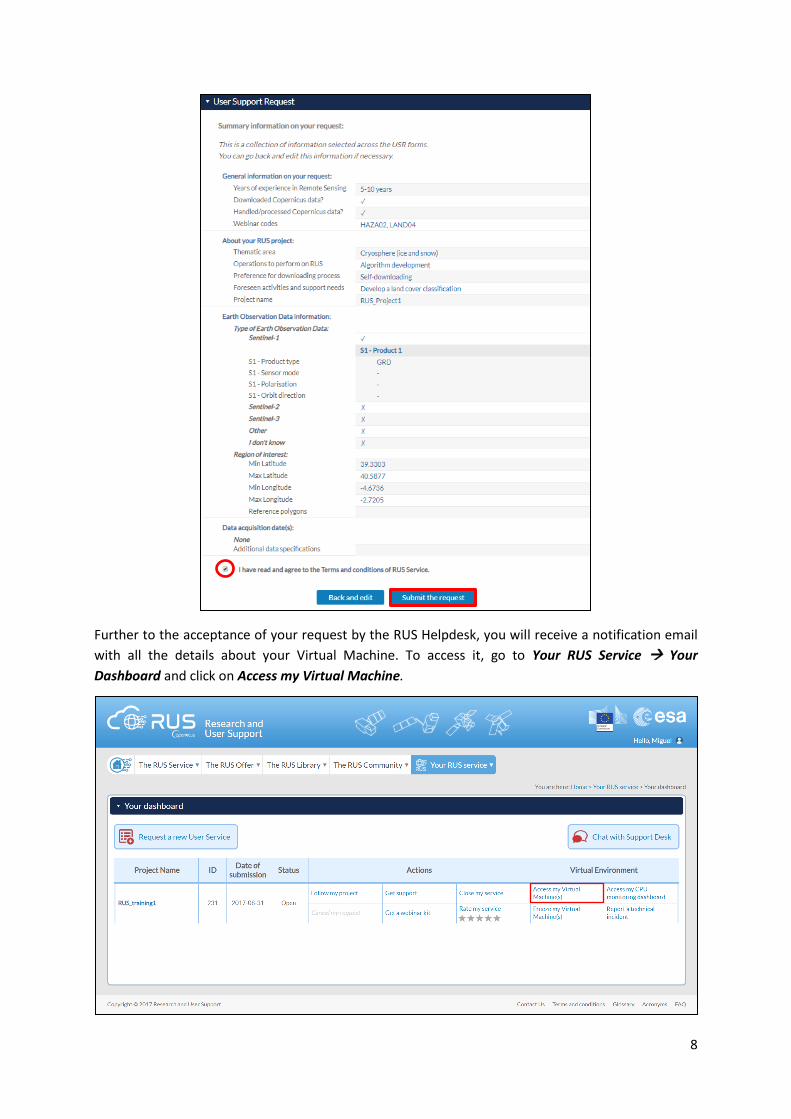
Complete the remaining steps, check the terms and conditions of the RUS Service and submit your
request once you are finished.
8
Further to the acceptance of your request by the RUS Helpdesk, you will receive a notification email
with all the details about your Virtual Machine. To access it, go to Your RUS Service → Your
Dashboard and click on Access my Virtual Machine.

9
Fill in the login credentials that have been provided to you by the RUS Helpdesk via email to access
your RUS Copernicus Virtual Machine.
This is the remote desktop of your Virtual Machine.

10
6 Step by step
6.1 Data download – ESA SciHUB
Before starting the exercise, make sure you are registered in the Copernicus Open Access Hub so that
you can access the free data provided by the Sentinel satellites.
Go to https://scihub.copernicus.eu/
Go to Open Hub. If you do not have an account, sign up in the upper right corner, fill in the details
and click register.
You will receive a confirmation email on the e-mail address you have specified: open the email and
click on the link to finalize the registration.
Once your account is activated – or if you already have an account – log in.
6.2 Download data
In this exercise, we will analyze 10 Sentinel-1A images during 2018. The following table shows the
date and reference of the images that will be used:

11
To improve the data acquisition process, we will use a download manager (See NOTE 1) that will
take care of downloading all products that will be used in this exercise. The metadata of the Sentinel
products are contained in a products.meta4 file created using the ‘Cart’ option of the Copernicus
Open Access Hub.
The products.meta4 file containing the links to the Sentinel-1 products to be downloaded can be
created following the methodology explained in NOTE 2. Follow the instructions and create your
cart file, download it and save it in the following path:
Path: /shared/Training/LAND06_UrbanClassification_Germany/Original/
Before using the downloading manager and the .meta4 file, let’s test if aria2 is properly installed in
the Virtual Machine. To do this, open the Command Line (in the bottom of your desktop window)
and type the following and press Enter:
aria2c
If aria2 is properly installed, the response should be as follows. If the response is ‘-bash aria2c:
command not found’ it means aria2 is not installed (See NOTE 3).
SATELLITE DATE IMAGE ID
Sentinel-1A
2018-04-12 S1A_IW_SLC__1SDV_20180412T171648_20180412T171715_021437_024E95_BDA1
2018-04-24 S1A_IW_SLC__1SDV_20180424T171648_20180424T171715_021612_02540A_BB21
2018-05-06 S1A_IW_SLC__1SDV_20180506T171649_20180506T171716_021787_025996_98AB
2018-05-18 S1A_IW_SLC__1SDV_20180518T171649_20180518T171716_021962_025F27_A15C
2018-05-30 S1A_IW_SLC__1SDV_20180530T171650_20180530T171717_022137_0264C8_5D94
2018-06-11 S1A_IW_SLC__1SDV_20180611T171651_20180611T171718_022312_026A3D_BBFC
2018-06-23 S1A_IW_SLC__1SDV_20180623T171652_20180623T171719_022487_026F7C_450E
2018-07-05 S1A_IW_SLC__1SDV_20180705T171652_20180705T171719_022662_027499_1B8F
2018-07-17 S1A_IW_SLC__1SDV_20180717T171653_20180717T171720_022837_0279EC_5E5E
2018-07-29 S1A_IW_SLC__1SDV_20180729T171654_20180729T171721_023012_027F72_97F6
NOTE 1: A download manager is a computer program dedicated to the task of downloading possibly
unrelated stand-alone files from (and sometimes to) the Internet for storage. For this exercise, we will
use aria2. Aria2 is a lightweight multi-protocol & multi-source command-line download utility. More
info at: https://aria2.github.io/

12
Once aria2 is ready to use, we can start the download process. For that, we need to navigate to the
folder where the products.meta4 is stored. Type the following command in the terminal and run it.
cd /shared/Training/LAND06_UrbanClassification_Germany/Original/
Next, type the following command (in a single line) to run the download tool. Replace username and
password (keep the quotation marks) with your login credentials for Copernicus Open Access Hub
(COAH). Do not clear your cart in the COAH until the download process is finished.
aria2c --http-user='username' --http-passwd='password' --check-certificate=
false --max-concurrent-downloads=2 -M products.meta4
The Sentinel products will be saved in the same path where the products.meta4 is stored.
NOTE 2: The Copernicus Open Access Hub allows you to add products to a ‘Cart’. For that, perform a
query; select the desired products from the result list and click on the ‘Add Product to Cart’ icon - . To
find the appropriate images, copy-paste the image ID specified in the table (pg. 11) in the search box of
the Copernicus Open Access Hub.
To view the products present in the cart just click anytime on the User Profile icon on top right corner of
the screen and then on "Cart". To download the cart click on "Download Cart" on the bottom right of
the page. A download window will pop up, asking the user confirmation to save a .meta4 file named
‘products.meta4’. This file contains all the metalinks of the products.
NOTE 3: If (and only if) the response is ‘-bash aria2c: command not found’, you need to install aria2. In
the command line, type: sudo apt-get install aria2
When requested, type: Y
Once finished, test the installation as explanied before.
13
6.3 Sentinel-1 SNAP Preprocessing
Once the Sentinel-1 images are downloaded, we need to run some pre-processing steps before they
can be used for the classification. For this purpose, we will use the SNAP software. In Applications ->
Processing open SNAP Desktop; click Open product , navigate to the following path and open the
two first S1 images (2018-04-12 and 2018-04-24)
Path: /shared/Training/LAND06_UrbanClassification_Germany/Original/
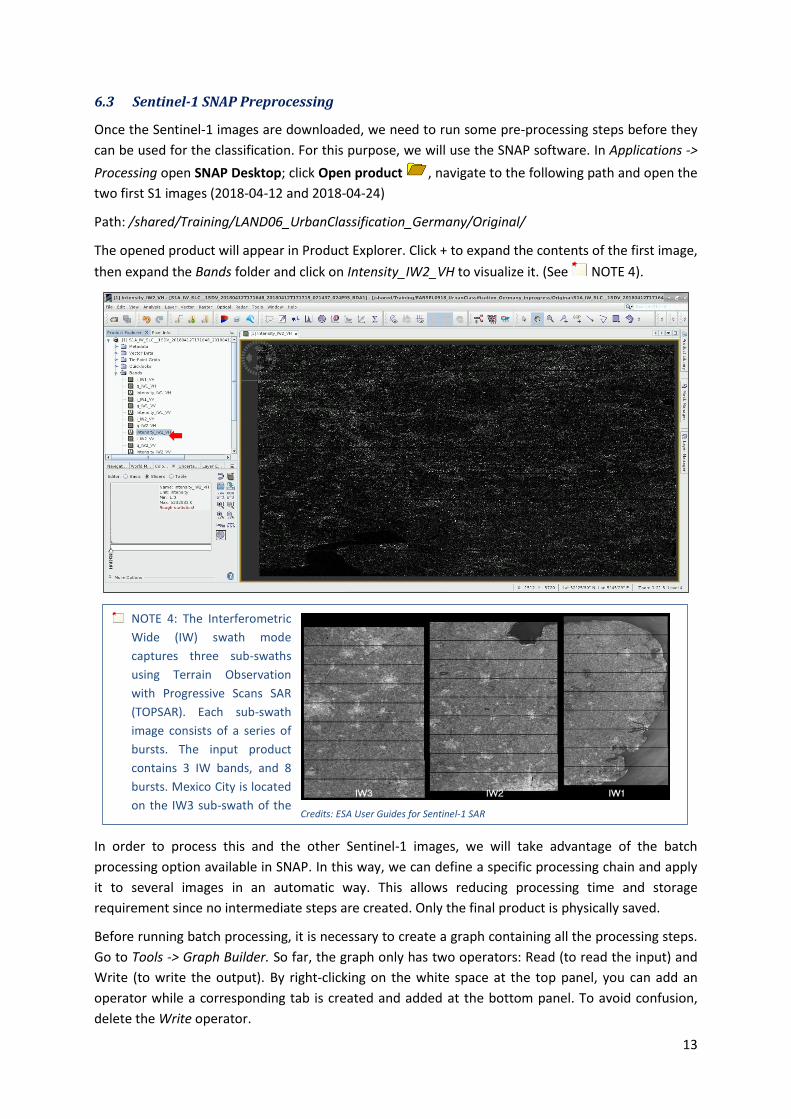
The opened product will appear in Product Explorer. Click + to expand the contents of the first image,
then expand the Bands folder and click on Intensity_IW2_VH to visualize it. (See NOTE 4).
In order to process this and the other Sentinel-1 images, we will take advantage of the batch
processing option available in SNAP. In this way, we can define a specific processing chain and apply
it to several images in an automatic way. This allows reducing processing time and storage
requirement since no intermediate steps are created. Only the final product is physically saved.
Before running batch processing, it is necessary to create a graph containing all the processing steps.
Go to Tools -> Graph Builder. So far, the graph only has two operators: Read (to read the input) and
Write (to write the output). By right-clicking on the white space at the top panel, you can add an
operator while a corresponding tab is created and added at the bottom panel. To avoid confusion,
delete the Write operator.
Credits: ESA User Guides for Sentinel-1 SAR
NOTE 4: The Interferometric
Wide (IW) swath mode
captures three sub-swaths
using Terrain Observation
with Progressive Scans SAR
(TOPSAR). Each sub-swath
image consists of a series of
bursts. The input product
contains 3 IW bands, and 8
bursts. Mexico City is located
on the IW3 sub-swath of the
Sentinel-1 images.

14
6.3.1 Read
In this analysis, we will derive coherence using as input two independent Sentinel-1A products. Due
to this, we need to add a second Read operator. For that, right click and go to Add -> Input-Output ->
Read. ). The corresponding tabs are created and added on the bottom panel. In the first Read tab set
the first image ([1] – 2018-04-12) as input. In the second Read(2) tab, set the second image ([2] –
2018-04-24) as input.
6.3.2 TOPSAR-Split
Since the area of interest is included in 2 bursts of the Sentinel-1 image, there is no need to process
the whole sub-swath with the 8 bursts (See NOTE 5). The extraction of Sentinel-1 TOPSAR bursts
will be made per acquisition and per sub-swath. This process will reduce the processing time in the
following processing steps and it is recommended when the analysis is focused only over a specific
area. To add the TOPSAR-Split operators, right click and go to Add -> Radar -> Sentinel-1 TOPS ->
TOPSAR-Split. Connect the operators as shown below by clicking to the right side of the Read
operator and dragging the red arrow towards the TOPSAR-Split operator.
In the TOPSAR-Split tabs, make sure to select the following parameters:
- Subswath: IW2
- Bursts: 1 to 2 (To do so, click on and drag it to the left until you reach Burst 2)
Do not click on any polarization. By default both are selected.
NOTE 5: The extraction of bursts in a sub-swath covering the area of interest may differ in Sentinel-1
images acquired on different dates.

15
6.3.3 Apply Orbit File
Next, we will update the orbit metadata (See NOTE 6) of the product to provide accurate satellite
position and velocity information. To add the operators to our graph, right click and go to Add ->
Radar -> Apply-Orbit-File. Connect the Apply-Orbit-File operators as shown below.
In the corresponding tabs, keep the default settings and click the option Do not fail if new orbit file is
not found.
6.3.4 Back Geocoding
Now we will co-registers the two S-1 SLC split products (master and slave) of the same sub-swath
using the orbits of the two products and a Digital Elevation Model (DEM). To add the operator, go to
Add-> Radar -> Corregistration -> S1 TOPS Corregistration -> Back-Geocoding. Set the two Apply Orbit
File operators as input. In the corresponding parameters tab, leave the default values.
NOTE 6: The orbit state vectors provided in the metadata of a SAR product are generally not accurate
and can be refined with the precise orbit files, which are available days-to-weeks after the generation
of the product. The orbit file provides accurate satellite position and velocity information. Based on this
information, the orbit state vectors in the abstract metadata of the product are updated. (SNAP Help)

16
6.3.5 Enhanced Spectral Diversity
This operator first estimates a constant range offset for the whole sub-swath of the split S-1 SLC
image using incoherent cross-correlation. Then, estimates a constant azimuth offset for the whole
sub-swath using an Enhanced Spectral Diversity (ESD) method. Finally, it performs range and azimuth
corrections for every burst using the range and azimuth offsets previously estimated. Right click and
go to Radar -> Coregistration -> S-1 TOPS coregistration -> Enhanced-Spectral-Diversity. Connect the
Back-Geocoding operator as shown below and leave all the parameters as default in the Enhanced-
Spectral-Diversity tab.
6.3.6 Coherence
Next, we will add the operator to derive the coherence image (See NOTE 7). Right click and go to
Add -> Radar -> Interferometric -> Products -> Coherence. Connect the Coherence operator as shown
below, select the option Subtract flat-earth phase and change the Square pixel parameter to 20.

17
6.3.7 TOPSAR Deburst
We continue the processing steps with Sentinel-1 TOPSAR Deburst. We have seen that each sub-
swath image consists of a series of bursts, where each burst has been processed as a separate SLC
image. The individually focused complex burst images are included, in azimuth-time order, into a
single sub-swath image with black-fill demarcation in between. There is sufficient overlap between
adjacent bursts and between sub-swaths to ensure the continuous coverage of the ground. The
images for all bursts in all sub-swaths are resampled to a common pixel spacing grid in range and
azimuth while preserving the phase information.
To add the TOPSAR-Deburst operator, go to Add -> Radar -> Sentinel-1 TOPS -> TOPSAR-Deburst. In
the TOPSAR-Deburst tab, select Polarizations: VV. Connect the Coherence operator as shown below
and keep all the parameters as default.
6.3.8 Multi-look
As the original SAR image contains inherent speckle noise, multilook processing is applied at this
moment to reduce the speckle appearance and to improve the image interpretability. To add the
Multilook operator go to Add -> Radar -> Multilook. Connect it to the TOPSAR-Deburst operator and
keep the default parameters.
NOTE 7: Coherence is the fixed relationship between waves in a beam of electromagnetic (EM)
radiation. Two wave trains of EM radiation are coherent when they are in phase. That is, they vibrate in
unison. In terms of the application to things like RADAR, the term coherence is also used to describe
systems that preserve the phase of the received signal.

18
6.3.9 Terrain correction
Our data are still in radar geometry, moreover due to topographical variations of a scene and the tilt
of the satellite sensor, the distances can be distorted in the SAR images. Therefore, we will apply
terrain correction to compensate for the distortions and reproject the scene to geographic projection
(See NOTE 8). To add the operator to our graph, right click and go to Add -> Radar -> Geometric ->
Terrain Correction -> Terrain-Correction. Connect it to the Multilook operator, change the pixel
spacing to 15 at the corresponding tab and make sure you select UTM / WGS 84 (Automatic) as Map
Projection.
NOTE 8: The geometry of topographical distortions in SAR
imagery is shown on the right. Here we can see that point B
with elevation h above the ellipsoid is imaged at position B’ in
SAR image, though its real position is B". The offset Δr
between B' and B" exhibits the effect of topographic
distortions. (SNAP Help)

19
6.3.10 Subset
Next, we need to reduce the spatial extent to focus on our study area. For that, add the Subset
operator. Right-click and go to Add -> Raster -> Geometric -> Subset. Connect it to the Terrain-
Correction operator. Select the option Geographic Coordinates and copy/paste the following
coordinates in Well-Known-Text format. Click Update to load them and Zoom in to the area.
POLYGON ((7.883054797352848 52.37328212685329, 8.210910785692109 52.37592581845208,
8.214610329430705 52.1670955892227, 7.888290792013983 52.16447160649477,
7.883054797352848 52.37328212685329))
6.3.11 Write
Finally, we need to properly save the output. For that, we first need to add the Write operator to our
graph. Right click and go to Add -> Input-Output -> Write. Connect the Write operator to the Subset
operator. In the Write tab, make sure you set the following name and directory.
Name: Coherence_20180412_20180424
Path: /shared/Training/LAND06_UrbanClassification_Germany/Processing/
Zoom in

20
Once finished, click on the Save icon. Navigate to the following path and save the graph as
1_S1_Splt_Orb_Cor_Coh_Deb_ML_TC.xml. Then, click Run to start the processing. It can take some
time depending on your VM specifications (3 hours approx. in a 16GB RAM and 4 cores VM).
Path: /shared/Training/LAND06_UrbanClassification_Germany/AuxData/
6.4 Import vector data
To prepare the data for the classification, the shapefile of the training areas has to be imported.
Select the Coherence_20180412_20180424 product in the product explorer and go to Vector ->
Import -> ESRI Shapefile. Navigate to the following path and click Open after selecting all the files.
Click No in the import geometry dialog.
Path: /shared/Training/LAND06_UrbanClassification_Germany/AuxData/
Once the vector data have been imported, do not forget to save the changes. Right click on the
subset product (index [3]) and click on Save Product. The vector data folder of the subset product
should look like the following image. Expand the product and open the Vector Data folder to check it.
6.5 Random Forest Classification
For this exercise, the Random Forest classification algorithm will be used (See NOTE 9).

21
Click on Raster -> Classification -> Supervised Classification -> Random Forest Classifier
In the ProductSet-Reader tab, click on the symbol. Navigate to the following path and select the
coherence image as input (Coherence_20180412_20180424).
Path: /shared/Training/LAND06_UrbanClassification_Germany/Processing/
Move to the Random-Forest-Classifier tab and set the following parameters:
- Uncheck the Evaluate classifier option
- Set the number of trees to 500
- Select all the shapefiles as training vectors
- Select all the bands as feature bands
NOTE 9: The Random Forest algorithm is a machine learning
technique that can be used for classification or regression. In
opposition to parametric classifiers (e.g. Maximum Likelihood), a
machine learning approach does not start with a data model but
instead learns the relationship between the training and the
response dataset. The Random Forest classifier is an aggregated
model, which means it uses the output from different models
(trees) to calculate the response variable.
Decision trees are predictive models that recursively split a dataset into regions by using a set of binary
rules to calculate a target value for classification or regression purposes. Given a training set with n
number of samples and m number of variables, a random subset of samples n is selected with
replacement (bagging approach) and used to construct a tree. At each node of the tree, a random
selection of variables m is used and, out of these variables, only the one providing the best split is used to
create two sub-nodes.
By combining trees, the forest is created. Each pixel of a satellite image is classified by all the trees of the
forest, producing as many classifications as number of trees. Each tree votes for a class membership and
then, the class with the maximum number of votes is selected as the final class.
More information about Random Forest can be found in Breiman, 2001.

22
Click now on the Write tab, set the Output folder to the following path, and specify the output name
according to the number of coherence images used: Classification_1_Coherence. Finally, click Run.
Path: /shared/Training/LAND06_UrbanClassification_Germany/Processing/
To visualize the result, expand the Bands folder in the Classification_1_Coherence product and
double click on LabelledClasses. You can change the colours by clicking on the Colour Manipulation
tab located in the lower left corner or by clicking on View -> Tool Windows -> Colour manipulation.
Select your own colours or click on the ‘Import colour palette’ icon ( ). Navigate to the following
path and select the RF_Colour.cpd file.
Path: /shared/Training/LAND06_UrbanClassification_Germany/AuxData/

23
7 Extra Steps
7.1 Coherence images
The result produced by using a single coherence image can be improved if more coherence products
are used for the classification. For this, we first have to produce them by following the same
approach as before. In SNAP, close all previous products, go to File -> Open product, navigate to the
following path and open the remaining 8 Sentinel-1 images that have not been used before. (2018-
05-06 | 2018-05-18 | 2018-05-30 | 2018-06-11 | 2018-06-23 | 20180705 | 20180717 | 20180729)
Path: /shared/Training/LAND06_UrbanClassification_Germany/Original/
Next, go to Tools -> GraphBuilder click on Load, navigate to the following path and open the
1_S1_Splt_Orb_Cor_Coh_Deb_ML_TC.xml graph file. Change the following parameters and click Run.
Remember that processing this graph may take some time depending on your VM specifications.
- Read tab → Make sure to select the Sentinel-1 product from 2018-05-06 (index [1]).
- Read(2) tab → Select the Sentinel-1 product from 2018-05-18 (index [2]).
- Write tab → Change the output name to Coherence_20180506_20180518

24
Once finished, repeat the same procedure for the remaining pair of images. Please note that since
this graph is computationally demanding, you may need to close and open SNAP in order to release
memory before processing a new pair of Sentinel-1 SLC products.
Read → 2018-05-30 [3] | Read(2) → 2018-06-11 [4] | Write → Coherence_20180530_20180611
Read → 2018-06-23 [5] | Read(2) → 2018-07-05 [6] | Write → Coherence_20180623_20180705
Read → 2018-07-17 [7] | Read(2) → 2018-07-29 [48] | Write → Coherence_20180717_20180729
After all the coherence images have been produced, close all the products in SNAP except for the 5
coherence images.
7.2 Create Stack
To use all the images as input for the Random Forest classification, we first need to stack all the
products together. For that, go to Radar -> Corresgistration -> Stack Tools -> Create Stack. In the
ProductSet-Reader tab, click at the icon to add the opened products. Click also at the icon to
update the metadata information.

25
Move now to the CreateStack tab and set the following parameters and click on the Find Optimal
Master button.
- Resampling type: NEAREST_NEIGHBOR
- Initial offset method: Product Geolocation
In the Write tab, change the output name to Coherence_Stack and make sure the output directory is
set to the following path and then click Run.
Path: /shared/Training/LAND06_UrbanClassification_Germany/Processing/

26
7.3 Multi-temporal Random Forest classification
Once the images are stacked, we can use them as input for the classification. Click on Raster ->
Classification -> Supervised Classification -> Random Forest Classifier
In the ProductSet-Reader tab, click on the symbol. Navigate to the following path and select the
stacked product as input (Coherence_Stack).
Path: /shared/Training/LAND06_UrbanClassification_Germany/Processing/
Move to the Random-Forest-Classifier tab and set the following parameters:
- Uncheck the Evaluate classifier option
- Set the number of trees to 500
- Select all the shapefiles as training vectors
- Select all the bands as feature bands
Click now on the Write tab, set the Output folder to the following path, and specify the output name
according to the number of coherence images used: Classification_5_Coherence. Finally, click Run.
Path: /shared/Training/LAND06_UrbanClassification_Germany/Processing/
To visualize the result, expand the Bands folder in the Classification_5_Coherence product and
double click on LabelledClasses. You can change the colours by clicking on the Colour Manipulation
tab located in the lower left corner or by clicking on View -> Tool Windows -> Colour manipulation.

27
Select your own colours or click on the ‘Import colour palette’ icon ( ). Navigate to the following
path and select the file RF_Colour.cpd.
Path: /shared/Training/LAND06_UrbanClassification_Germany/AuxData/
THANK YOU FOR FOLLOWING THE EXERCISE!
8 Further reading and resources
Sentinel-1 User Guide
https://sentinel.esa.int/web/sentinel/user-guides/sentinel-1-sar
Sentinel-1 Technical Guide
https://sentinel.esa.int/web/sentinel/technical-guides/sentinel-1-sar
InSAR Principles – ESA
http://www.esa.int/About_Us/ESA_Publications/InSAR_Principles_Guidelines_for_SAR_Interferometry_Processing_and_In
terpretation_br_ESA_TM-19
Breiman, L. (2001). Random Forests. Machine Learning, 45, 5–32, 45(1), 5–32.
FOLLOW US!!!
RUS-Copernicus website
website
RUS-Copernicus Training website
RUS Copernicus Training
@RUS-Copernicus
RUS-Copernicus
RUS-Copernicus


