Updated portfolio skills october 2015

1

Jordan Lisa Rose

Technical and Transferable Laboratory Skills Portfolio

Bio-science

2

Portfolio Index

Page number

Page title Portfolio skills (P1-P11)

Numerical representation of skills in each portfolio

3-5 P1 - Cell culture of INS-1 cell line 1,2,4,6,21,27,30,31,32

6-7 P2 - Immunofluorescence microscopy 1,6,17,23,24,27,30,32,33

8-11 P3 - Viral inoculation of tissue culture 1,2,3,5,6,11,20,27,28,30,31

12-16 P4 - PBMC separation and blood film preparation 3,5,6,18,19,27,28,29,30

17-20 P5 - Using an automated FBC analyser and interpreting results 6,11,27,33,34,

21-25 P6 - Enzyme-linked Immunosorbant assay (ELISA) 6,7,13,23,27,28,30,38

36-28 P7 - Assessing the GMO status of a plant food 6,14,15,16,22,27,30,31,33

29-33 P8 - Screening for inborn errors of metabolism 12,11,14,27,35,39

34-38 P9 - Precipitation techniques in agar 6,25,26,27,28,30,38

39-42 P10 - Sensitisation of smooth muscle tissue 10,11,27,28,30,37,38

43-45 P11 - Scientific poster presentation 8,9,29,36,40

Bioscience skills numbered 1-26

Culturing mammalian cells 1 Using positive and negative controls 14 Microscopy 2 Carrying out PCR 15

Using a haemocytometer 3 Carrying out agarose gel electrophoresis 16 Preparation of appropriate growth mediums 4 Preparing a secretagoge 17

Centrifugation 5 Isolation of PBMCs 18 Correct use of a pipettor/automated pipette 6 Making blood films 19

Carrying out an ELISA 7 Using a quantal assay 20 Research, analyse and critique journals 8 Preparation of PBS 21

Understand/explain complex scientific concepts 9 Visualising results using gel documentation 22 Set up and use of a gut bath 10 Using antibodies 23

Safe handling of bio-hazardous material 11 Immunofluorescence microscopy 24 The use of TLC 12 Making serial dilutions 25

Preparing dilutions 13 Carrying out immunodiffusion assays 26

Transferable skills number 27-40

Use of PPE and aseptic technique 27 Following standard operating protocols 34 Data analysis 28 Using initiative 35

Communicating results in a formal report 29 Use of PowerPoint 36 Following a protocol 30 Use of Minitab (Statistical analysis) 37 Time management 31 Displaying data graphically 38

Team work 32 Tabulating results 39 Using a computer based storage system 33 Learn from feedback 40

3

Name: Jordan Rose Date: 27/06/14

Source: Summer placement

Experiment: Cell culture of rat insulinoma cells (INS-1 cell line)

Portfolio Skills:

Bioscience skills Transferable skills

1. Culturing mammalian cells 2. Correct use of a pipettor 3. Preparation of appropriate growth medium 4. Preparation of PBS 5. Microscopy

1. Use of PPE and aseptic technique 2. Following a protocol 3. Time management 4. Team work

Aim:

Successfully grow, study and check the viability of rat insulanoma cells (INS-1 cell line)

Summary of evidence

Cell culture is carried out in an aseptic environment (use 70% ethanol to clean surfaces), with correct fume hood

regulations such as maintaining laminar air flow, avoid cluttering and access to an appropriate system of disposal. An

appropriate cell medium (in this case RPMI culture media with 10% Foetal Bovine Serum (FBS)) and PBS must be prepared

in advance. Trypsin EDTA, sterile culture flasks, a pipettor and wrapped disposable pipettes should be placed in the fume

cupboard in advance to avoid contamination whilst working under the fume cupboard.

Cultures that are to be split are taken directly from a flask that has cells that are approximately 80% confluent (80% of

surface of flask covered by cell monolayer). Splitting is achieved by carefully pouring off the media into a waste pot, then

using a sterile pipette add trypsin EDTA until all the cells adhered to the bottom of the flask are covered (75 cm2 flask

needs approximately 5 ml of trypsin). The trypsin should detach the cells without damaging them and gentle tapping on

the flask will aid this. At this point, some fresh culture media should be added to the flask to inactivate the trypsin. This

cell suspension can then be pipetted into new flasks (for a 25cm2 flask add approximately 5-10 ml of cell suspension, and

for 75cm2 flask add approximately 10-30ml of cell suspension.) After this point, allow the cells to grow over night in an

incubator at 37oC to allow them to recover and settle.

Over the next week, feed the cells by gently pouring media out of the flask (cells that are healthy should be adhered and

not dislodge and fall out with media) and add fresh media that has previously been warmed at 37°C in water bath for at

least 30 min. The flasks should be regularly checked via microscopy to monitor condition and growth. Once 80% confluent

is reached again, repeat the process of splitting the cells into new flasks.

BIOSCIENCE PORTFOLIO

4

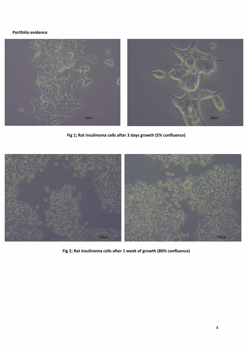
Portfolio evidence

Fig 1; Rat insulinoma cells after 3 days growth (5% confluence)

Fig 2; Rat insulinoma cells after 1 week of growth (80% confluence)

20µm 20µm

100µm

100µm

5

Reflection

Cell culture is a fundamental process in many areas of research. Rat insulinoma cells (INS-1) are used in the research of

diabetes due to their high insulin content and their excellent responsiveness to glucose. During this procedure, the

original cells that were split went on to remain healthy and viable. They were regularly split and used throughout the lab

as the basis for a range of procedures.

There was one incident of contamination though where a 25ml flask had to be discarded. This was noticed via microscopy

where a foreign body was spotted floating in the media. This meant that the cells in this particular flask where now

compromised and therefore unsuitable for use. This proved the importance of regular checks on the growth and state of

the cell culture and why aseptic technique is important.

Some insulinoma cells seemed to also produce a strange black substance significantly smaller than the cell itself. This was

later discovered to be due to the stress of moving the flasks too much and checking them far too often. Being particularly

gentle with the flasks seemed to reverse this problem though as once the cells were content again the black substance

disappeared.

6


Source: Summer placement

Experiment: Immunofluorescence Microscopy

Portfolio Skills:

Aim:

Prepping the cells by adding antibodies to them (primary – Goat abs and rabbit abs. Secondary – donkey anti-goat and donkey anti-rabbit abs) and properly storing the cells.

Use of the confocal laser scanning microscopy to view images of fluorescing proteins and identify the proteins Calpain 10 and Snap 25.

Summary of evidence

In order to study the proteins within the INS-1 cell line insulinoma cells, it is initially important to culture the cells and

make sure they are healthy. They are then split from their culture containers and added to a six-well plate which has a

sterile glass coverslip within each well. The cells will then grow and adhere, in the presence of a specially made

secretagoge, over the next 24 hours. These cells are then washed with PBS the next day and fixated by incubating the

cells in 100% methanol (chilled at -20°C) at room temperature for 5 minutes. DAPI is used to stain the nucleus of each cell

and a blocking solution is added before the addition of primary antibodies (Goat ab and rabbit ab) that will each bind to

Calpain 10 and Snap 25. Next secondary abs are added which will bond to the primary abs. Donkey anti-goat abs will bond

to the goat abs and fluoresce green when viewed through the confocal microscope, and the donkey anti-rabbit abs will

bond to rabbit abs and fluoresce red under the confocal microscope. This glass disk is then lifted carefully out of the well

using tweezers and studied to see which proteins are present.

Results

Calpain 10 = fluoresced green

Snap 25 = fluoresced red

Co-localisation of proteins = fluoresced orange


1. Cell culture 2. Correct use of a pipettor/automated

pipette 3. Preparing a secretagoge 4. Using primary and secondary antibodies 5. immunofluorescence microscopy

1. Use of PPE and aseptic technique 2. Following a protocol 3. Using a computer based storage system 4. Team work


7

Portfolio Evidence

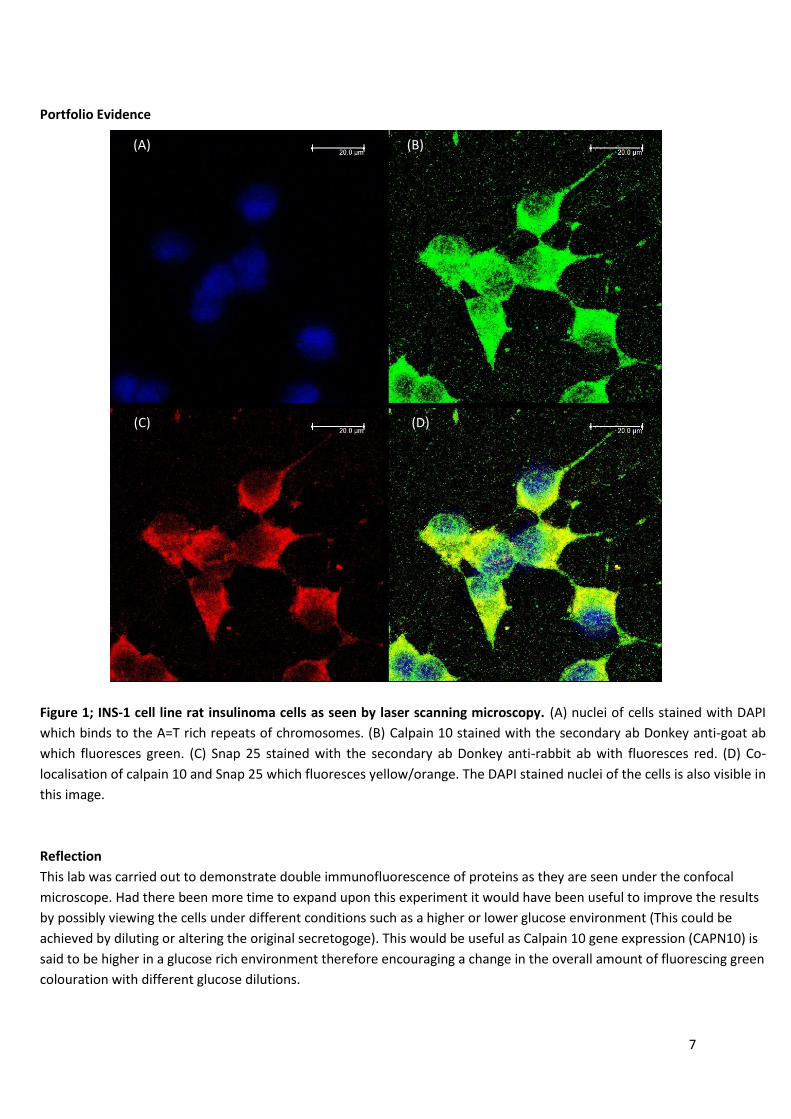
Figure 1; INS-1 cell line rat insulinoma cells as seen by laser scanning microscopy. (A) nuclei of cells stained with DAPI

which binds to the A=T rich repeats of chromosomes. (B) Calpain 10 stained with the secondary ab Donkey anti-goat ab

which fluoresces green. (C) Snap 25 stained with the secondary ab Donkey anti-rabbit ab with fluoresces red. (D) Co-

localisation of calpain 10 and Snap 25 which fluoresces yellow/orange. The DAPI stained nuclei of the cells is also visible in

this image.

Reflection

This lab was carried out to demonstrate double immunofluorescence of proteins as they are seen under the confocal

microscope. Had there been more time to expand upon this experiment it would have been useful to improve the results

by possibly viewing the cells under different conditions such as a higher or lower glucose environment (This could be

achieved by diluting or altering the original secretogoge). This would be useful as Calpain 10 gene expression (CAPN10) is

said to be higher in a glucose rich environment therefore encouraging a change in the overall amount of fluorescing green

colouration with different glucose dilutions.

(A) (B)

(D) (C)

8


Source: Immunology and virology

Experiment: Viral inoculation of a tissue culture

Portfolio Skills:


6. Culturing mammalian cells 7. Correct use of a pipettor 8. Handling bio-hazardous material with care 9. Microscopy 10. Counting viable cells using trypan blue and a

haemocytometer 11. The use of a quantal assay

1. Use of PPE and aseptic technique 2. Following a protocol 3. Time management 4. Data Analysis 5. Communicating results in a formal lab report

Aim:

Overseeing the growth, maintenance, viability and splitting of a cell culture (Rhesus monkey kidney cells), as well as overseeing the addition and growth of a virus within this cell culture.

Harvest the virus and add dilutions of the mixture (10-1 to 10-10) to a 96 well plate.

Use TCID50 to count the number of infectious virus particles based on cytopathic effect (CPE).

Use the Reed and Muench (1938) mathematical technique to determine the percentage of infection and to calculate the 50% end point, before determining viral titre.

Summary of evidence

Rhesus monkey kidney cells were cultured and infected with herpes virus. The virus was then harvested by centrifugation

and sonification of the cells. A serial dilution of the sample was then carried out (10-1 to 10-10) and then the dilutions were

seeded into a 96 well plate. TCID50, which is a quantal assay, was used to count the number of infectious virus particles

based on the presence of cytopathic effect (CPE) of the cells. This CPE could be displayed as rounding of the cells, syncytia

of adjacent cells, or the appearance of inclusion bodies. Once this information was gained the Reed and Muench (1938)

mathematical technique was used to determine the percentage of infection within cells and used to calculate the 50%

end point to determine viral titre.

Results

End point dilution that infects 50% of the cell cultures inoculated is 10-4.

The viral titre was 105.16 ID50/ml


9

Portfolio evidence

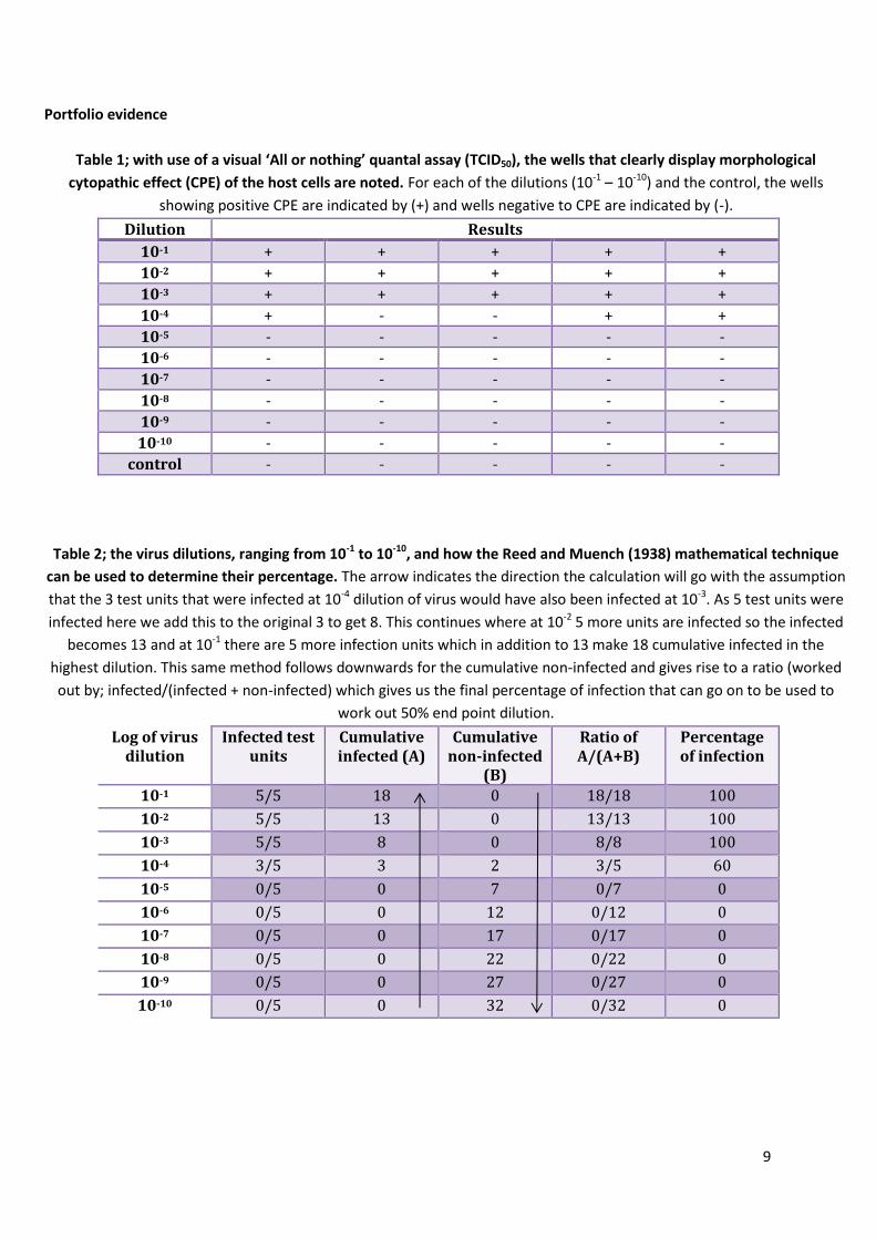
Table 1; with use of a visual ‘All or nothing’ quantal assay (TCID50), the wells that clearly display morphological

cytopathic effect (CPE) of the host cells are noted. For each of the dilutions (10-1 – 10-10) and the control, the wells

showing positive CPE are indicated by (+) and wells negative to CPE are indicated by (-).

Dilution Results

10-1 + + + + +

10-2 + + + + +

10-3 + + + + +

10-4 + - - + +

10-5 - - - - -

10-6 - - - - -

10-7 - - - - -

10-8 - - - - -

10-9 - - - - -

10-10 - - - - -

control - - - - -

Table 2; the virus dilutions, ranging from 10-1 to 10-10, and how the Reed and Muench (1938) mathematical technique

can be used to determine their percentage. The arrow indicates the direction the calculation will go with the assumption

that the 3 test units that were infected at 10-4 dilution of virus would have also been infected at 10-3. As 5 test units were

infected here we add this to the original 3 to get 8. This continues where at 10-2 5 more units are infected so the infected

becomes 13 and at 10-1 there are 5 more infection units which in addition to 13 make 18 cumulative infected in the

highest dilution. This same method follows downwards for the cumulative non-infected and gives rise to a ratio (worked

out by; infected/(infected + non-infected) which gives us the final percentage of infection that can go on to be used to

work out 50% end point dilution.

Log of virus dilution

Infected test units

Cumulative infected (A)

Cumulative non-infected

(B)

Ratio of A/(A+B)

Percentage of infection

10-1 5/5 18 0 18/18 100

10-2 5/5 13 0 13/13 100

10-3 5/5 8 0 8/8 100

10-4 3/5 3 2 3/5 60

10-5 0/5 0 7 0/7 0

10-6 0/5 0 12 0/12 0

10-7 0/5 0 17 0/17 0

10-8 0/5 0 22 0/22 0

10-9 0/5 0 27 0/27 0

10-10 0/5 0 32 0/32 0

10

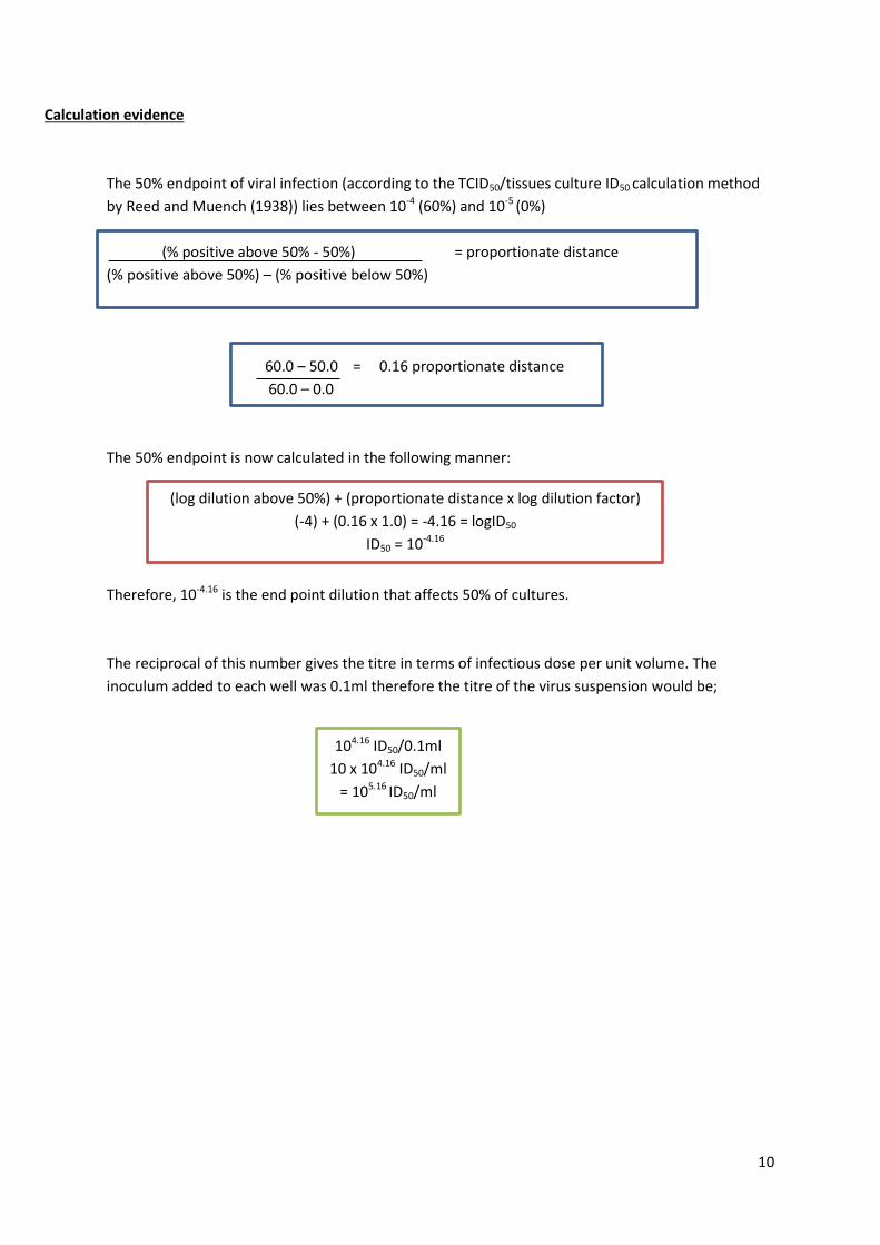
Calculation evidence

The 50% endpoint of viral infection (according to the TCID50/tissues culture ID50 calculation method

by Reed and Muench (1938)) lies between 10-4 (60%) and 10-5 (0%)

(% positive above 50% - 50%) = proportionate distance

(% positive above 50%) – (% positive below 50%)

60.0 – 50.0 = 0.16 proportionate distance

60.0 – 0.0

The 50% endpoint is now calculated in the following manner:

Therefore, 10-4.16 is the end point dilution that affects 50% of cultures.

The reciprocal of this number gives the titre in terms of infectious dose per unit volume. The

inoculum added to each well was 0.1ml therefore the titre of the virus suspension would be;

104.16 ID50/0.1ml

10 x 104.16 ID50/ml

= 105.16 ID50/ml

(log dilution above 50%) + (proportionate distance x log dilution factor)

(-4) + (0.16 x 1.0) = -4.16 = logID50

ID50 = 10-4.16

11

Reflection

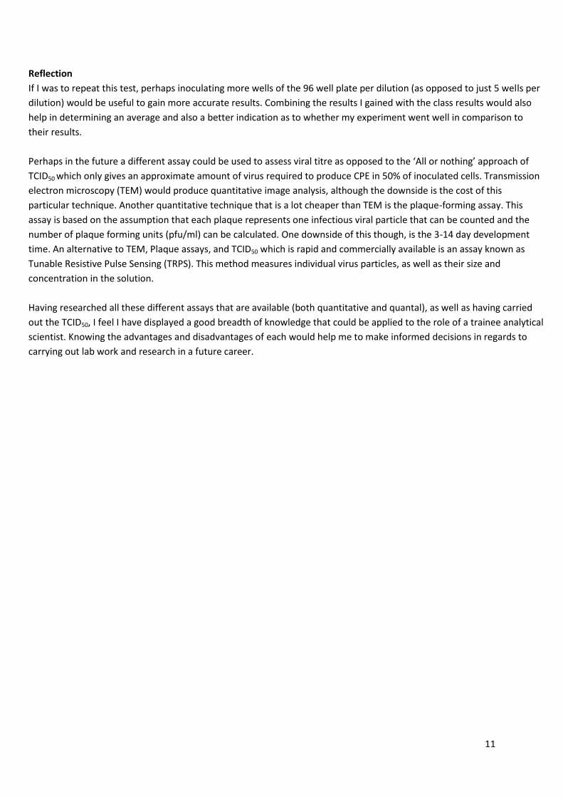
If I was to repeat this test, perhaps inoculating more wells of the 96 well plate per dilution (as opposed to just 5 wells per

dilution) would be useful to gain more accurate results. Combining the results I gained with the class results would also

help in determining an average and also a better indication as to whether my experiment went well in comparison to

their results.

Perhaps in the future a different assay could be used to assess viral titre as opposed to the ‘All or nothing’ approach of

TCID50 which only gives an approximate amount of virus required to produce CPE in 50% of inoculated cells. Transmission

electron microscopy (TEM) would produce quantitative image analysis, although the downside is the cost of this

particular technique. Another quantitative technique that is a lot cheaper than TEM is the plaque-forming assay. This

assay is based on the assumption that each plaque represents one infectious viral particle that can be counted and the

number of plaque forming units (pfu/ml) can be calculated. One downside of this though, is the 3-14 day development

time. An alternative to TEM, Plaque assays, and TCID50 which is rapid and commercially available is an assay known as

Tunable Resistive Pulse Sensing (TRPS). This method measures individual virus particles, as well as their size and

concentration in the solution.

Having researched all these different assays that are available (both quantitative and quantal), as well as having carried

out the TCID50, I feel I have displayed a good breadth of knowledge that could be applied to the role of a trainee analytical

scientist. Knowing the advantages and disadvantages of each would help me to make informed decisions in regards to

carrying out lab work and research in a future career.

12


Source: Immunology and Virology

Experiment: PBMC separation and blood film preparation

Portfolio Skills:


1. Correct use of automated pipettes 2. Isolation of PBMCs from whole blood 3. Centrifugation 4. Using a haemocytometer to count cells 5. Preparation of blood films

1. Use of PPE and aseptic technique 2. Following a protocol 3. Data analysis 4. Communicating results in a formal lab report

Aims:

The careful isolation of Peripheral blood mononuclear cells (PBMCs) from a sample of whole blood.

Preparation of blood films (both whole blood and separated blood).

Using a haemocytometer to determine the white blood cell (WBC) count of whole blood, and calculating the viable count of separated PBMC in cell suspension.

Summary of work

The purpose of this lab was to carefully and accurately separate PBMCs from a sample of whole blood. This was achieved

using density gravity sedimentation via Isopaque-Ficoll mixture, centrifugation and accurate pipetting technique to

extract the PBMC ‘halo’. The whole blood and the separated sample of PBMCs were used to make blood films. Leishman’s

reagent was added to the slides to determine a differential count of the whole blood, and to show how accurate my

PBMC separation was. A haemocytometer was used to determine the WBC count of the whole blood and to calculate the

viable count of separated PBMCs in cell suspension. This information was then used for a series of calculations aimed at

determining the percentage recovery of my final PBMC cell suspension.

Results

The percentage recovery of PBMCs was 88.5%.


13

Portfolio evidence

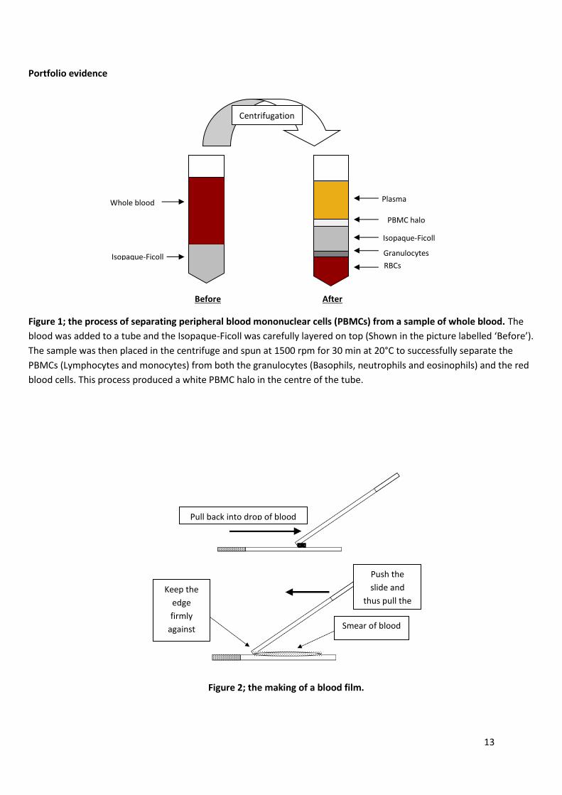
Figure 1; the process of separating peripheral blood mononuclear cells (PBMCs) from a sample of whole blood. The

blood was added to a tube and the Isopaque-Ficoll was carefully layered on top (Shown in the picture labelled ‘Before’).

The sample was then placed in the centrifuge and spun at 1500 rpm for 30 min at 20°C to successfully separate the

PBMCs (Lymphocytes and monocytes) from both the granulocytes (Basophils, neutrophils and eosinophils) and the red

blood cells. This process produced a white PBMC halo in the centre of the tube.

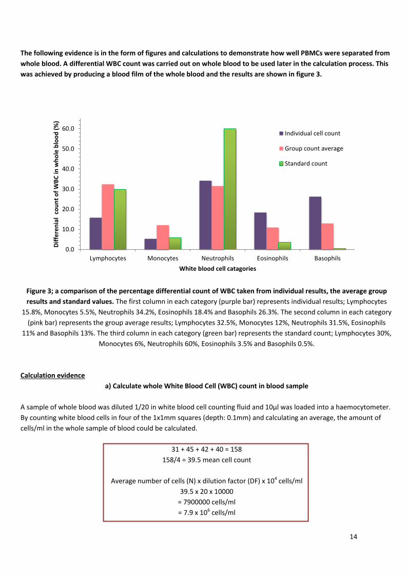
Figure 2; the making of a blood film.

Isopaque-Ficoll

Isopaque-Ficoll

Whole blood Plasma

PBMC halo

Granulocytes

RBCs

Before After

Centrifugation

Keep the

edge

firmly

against

the slide

Pull back into drop of blood

Push the

slide and

thus pull the

blood Smear of blood

14

The following evidence is in the form of figures and calculations to demonstrate how well PBMCs were separated from

whole blood. A differential WBC count was carried out on whole blood to be used later in the calculation process. This

was achieved by producing a blood film of the whole blood and the results are shown in figure 3.

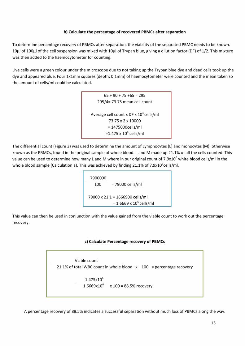
Figure 3; a comparison of the percentage differential count of WBC taken from individual results, the average group

results and standard values. The first column in each category (purple bar) represents individual results; Lymphocytes

15.8%, Monocytes 5.5%, Neutrophils 34.2%, Eosinophils 18.4% and Basophils 26.3%. The second column in each category

(pink bar) represents the group average results; Lymphocytes 32.5%, Monocytes 12%, Neutrophils 31.5%, Eosinophils

11% and Basophils 13%. The third column in each category (green bar) represents the standard count; Lymphocytes 30%,

Monocytes 6%, Neutrophils 60%, Eosinophils 3.5% and Basophils 0.5%.

Calculation evidence

a) Calculate whole White Blood Cell (WBC) count in blood sample

A sample of whole blood was diluted 1/20 in white blood cell counting fluid and 10µl was loaded into a haemocytometer.

By counting white blood cells in four of the 1x1mm squares (depth: 0.1mm) and calculating an average, the amount of

cells/ml in the whole sample of blood could be calculated.

31 + 45 + 42 + 40 = 158

158/4 = 39.5 mean cell count

Average number of cells (N) x dilution factor (DF) x 104 cells/ml

39.5 x 20 x 10000

= 7900000 cells/ml

= 7.9 x 106 cells/ml

0.0

10.0

20.0

30.0

40.0

50.0

60.0

Lymphocytes Monocytes Neutrophils Eosinophils Basophils

Dif

fere

nia

l co

un

t o

f W

BC

in w

ho

le b

loo

d (

%)

White blood cell catagories

Individual cell count

Group count average

Standard count

15

b) Calculate the percentage of recovered PBMCs after separation

To determine percentage recovery of PBMCs after separation, the viability of the separated PBMC needs to be known.

10µl of 100µl of the cell suspension was mixed with 10µl of Trypan blue, giving a dilution factor (DF) of 1/2. This mixture

was then added to the haemocytometer for counting.

Live cells were a green colour under the microscope due to not taking up the Trypan blue dye and dead cells took up the

dye and appeared blue. Four 1x1mm squares (depth: 0.1mm) of haemocytometer were counted and the mean taken so

the amount of cells/ml could be calculated.

65 + 90 + 75 +65 = 295

295/4= 73.75 mean cell count

Average cell count x DF x 104 cells/ml

73.75 x 2 x 10000

= 1475000cells/ml

=1.475 x 106 cells/ml

The differential count (Figure 3) was used to determine the amount of Lymphocytes (L) and monocytes (M), otherwise

known as the PBMCs, found in the original sample of whole blood. L and M made up 21.1% of all the cells counted. This

value can be used to determine how many L and M where in our original count of 7.9x106 white blood cells/ml in the

whole blood sample (Calculation a). This was achieved by finding 21.1% of 7.9x106cells/ml.

7900000

100 = 79000 cells/ml

79000 x 21.1 = 1666900 cells/ml

= 1.6669 x 106 cells/ml

This value can then be used in conjunction with the value gained from the viable count to work out the percentage

recovery.

c) Calculate Percentage recovery of PBMCs

Viable count

21.1% of total WBC count in whole blood x 100 = percentage recovery

1.475x106

1.6669x106 x 100 = 88.5% recovery

A percentage recovery of 88.5% indicates a successful separation without much loss of PBMCs along the way.

16

Reflection

Upon looking back at the lab, the differential counts greatly differed in my own results and the class results when

compared to the standard values. This was seen particularly in the neutrophils, eosinophils and basophils. A repeat of this

lab would be appropriate as it could either be due to the batch of blood that was used being high in this cells or it could

be down to inaccuracy of doing a manual count of differentials. Perhaps it would be worthwhile in the future to run

samples through an analyser to improve accuracy in this area.

This lab went better than expected in regards to gaining a high percentage recovery of PBMCs, but there is always room

for improvement. The use of a different separation technique would make the percentage recovery higher. A special

devise to make separation easier and more accurate could be used with one ne example of this being the BD Vacutainer®

cell preparation tube. This devise is vacuum-driven, contains anti-coagulant and a cell separation medium which is made

of polyester gel and a density gradient liquid. It can be used to draw blood and at the same time separate PBMCs within

the same tube. This would exclude the need for blood dilution or transfer to other containers which in turn could lead to

loss of PBMCs due to human error when using Isopaque-Ficoll, such as in this lab, which is highly operator dependant as it

has to be manually added and can cause unwanted variation to the percentage recovery rate.

17


Source: Project laboratory/haematology seminar

Experiment: Using an automated full blood count (FBC) analyser and analysing FBC results

Portfolio Skills:


1. Collection, handling and storage of human blood samples (bio-hazardous material)

2. Correct use of an automated pipette

1. Use of PPE and aseptic technique 2. Following standard operating

procedures (including quality control and changing reagents)

3. Using a computer based data storage system

Aim:

Collect blood from a healthy volunteer and analyse the sample (the sample may be diluted 7:1 using cell pack if not enough sample is readily available).

From example FBC data (Q1-3), interoperate the information and accurately diagnose the patient.

Summary of evidence

The proper use of the analyser was essential as well as following proper protocol when bringing in volunteers willing to

donate their blood. To demonstrate what results are expected from an automated full blood count analyser and to allow

for the diagnosis of certain disorders of the blood, the use of example data from a lab seminar was used in place of real

data. This was due to ethical approval of what was done with volunteer donations of blood and also the fact that all the

volunteers answered a health survey stating they were in fact healthy and ‘normal’, therefore little variation in the FBC

would be seen.

Suspected results

Sample 1 – Healthy female patient (False thrombocytopenia was seen due to clot in the sample)

Sample 2 – Microcytic anaemia

Sample 3 – Acute phase malaria


18

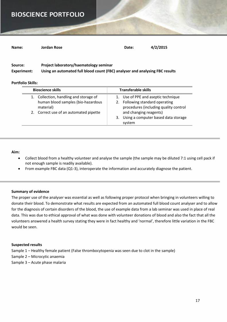
Portfolio Evidence

Figure 1; the proper collection of healthy blood samples and using the Sysmex XS 1000i automated analyser to gain a

full blood count. Spring activated lancets were used to prick the finger of a healthy volunteer and blood was collected in a

tube that contained EDTA to stop coagulation of the sample. Samples could be kept for up to a week at 4oC and analysed

using the Sysmex 1000i to gain a full blood count reading for the individual.

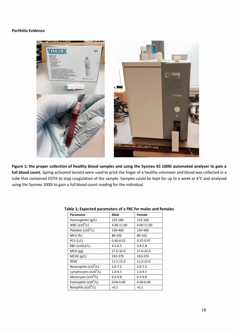
Table 1; Expected parameters of a FBC for males and females

Parameter Male Female

Haemoglobin (g/L) 135-180 115-160

WBC (x109/L) 4.00-11.00 4.00-11.00

Platelets (x109/L) 150-400 150-400

MCV (fL) 80-102 80-102

PCV (L/L) 0.40-0.52 0.37-0.47

RBC (x1012/L) 4.5-6.5 3.8-5.8

MCH (pg) 27.0-32.0 27.0-32.0

MCHC (g/L) 310-370 310-370

RDW 11.5-15.0 11.5-15.0

Neutrophils (x109/L) 2.0-7.5 2.0-7.5

Lymphocytes (x109/L) 1.0-4.5 1.0-4.5

Monocytes (x109/L) 0.2-0.8 0.2-0.8

Eosinophils (x109/L) 0.04-0.40 0.04-0.40

Basophils (x109/L) <0.1 <0.1

19

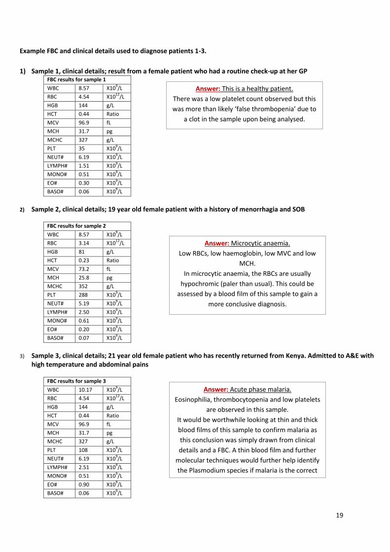
Example FBC and clinical details used to diagnose patients 1-3.

1) Sample 1, clinical details; result from a female patient who had a routine check-up at her GP FBC results for sample 1

WBC 8.57 X109/L

RBC 4.54 X1012

/L

HGB 144 g/L

HCT 0.44 Ratio

MCV 96.9 fL

MCH 31.7 pg

MCHC 327 g/L

PLT 35 X109/L

NEUT# 6.19 X109/L

LYMPH# 1.51 X109/L

MONO# 0.51 X109/L

EO# 0.30 X109/L

BASO# 0.06 X109/L

2) Sample 2, clinical details; 19 year old female patient with a history of menorrhagia and SOB

FBC results for sample 2

WBC 8.57 X109/L

RBC 3.14 X1012

/L

HGB 81 g/L

HCT 0.23 Ratio

MCV 73.2 fL

MCH 25.8 pg

MCHC 352 g/L

PLT 288 X109/L

NEUT# 5.19 X109/L

LYMPH# 2.50 X109/L

MONO# 0.61 X109/L

EO# 0.20 X109/L

BASO# 0.07 X109/L

3) Sample 3, clinical details; 21 year old female patient who has recently returned from Kenya. Admitted to A&E with high temperature and abdominal pains

FBC results for sample 3

WBC 10.17 X109/L

RBC 4.54 X1012

/L

HGB 144 g/L

HCT 0.44 Ratio

MCV 96.9 fL

MCH 31.7 pg

MCHC 327 g/L

PLT 108 X109/L

NEUT# 6.19 X109/L

LYMPH# 2.51 X109/L

MONO# 0.51 X109/L

EO# 0.90 X109/L

BASO# 0.06 X109/L

Answer: This is a healthy patient.

There was a low platelet count observed but this

was more than likely ‘false thrombopenia’ due to

a clot in the sample upon being analysed.

Answer: Microcytic anaemia.

Low RBCs, low haemoglobin, low MVC and low

MCH.

In microcytic anaemia, the RBCs are usually

hypochromic (paler than usual). This could be

assessed by a blood film of this sample to gain a

more conclusive diagnosis.

Answer: Acute phase malaria.

Eosinophilia, thrombocytopenia and low platelets

are observed in this sample.

It would be worthwhile looking at thin and thick

blood films of this sample to confirm malaria as

this conclusion was simply drawn from clinical

details and a FBC. A thin blood film and further

molecular techniques would further help identify

the Plasmodium species if malaria is the correct

diagnosis

20

Reflection

As only healthy samples were available (due to ethics concerning the use of human blood samples) there was no real

results generated to assess and diagnose. It would have been good practice to have the responsibility of working with

hospital samples but I feel the use of example FBC to practice diagnostic skills was adequate at this stage of

understanding the FBC analyser. As for the diagnosis of each of the 5 example patients using FBC results alone, coupling

this with looking at blood films would have helped to conclusively gained more accurate results.

The job application states that flow cytometry is a technique that will be carried out by the trainee analytical scientist.

During the time spent working with the automated haematological analyser I became very familiar with the machine and

came to understand its inner workings and therefore the concept behind flow cytometry. I feel this is adequate

background understanding and good practice for carrying out techniques of this nature in a professional setting.

21


Source: Antibody & DNA technology

Experiment: Enzyme-linked immunosorbent assay (ELISA)

Portfolio Skills:


1. Carrying out an ELISA 2. Making dilutions 3. Use of antibodies 4. Correct use of automated pipettes

1. Use of PPE and aseptic technique 2. Following a protocol 3. Data Analysis 4. Displaying data graphically

Aim:

Observe changes in the titre of antisera during the course of an immunisation schedule

Determine whether the antisera, taken after the third immunisation, is specific to human albumin

Evidence Review

During experiment 1, the titre will determine, from 3 antisera bleeds (bleed 1 - antiserum taken from a rabbit after first

immunisation, bleed 2 - antiserum taken after second immunisation and bleed 3 - antiserum taken after third

immunisation) which has the highest amount of antibody available to bond to human albumin. This will demonstrate an

effective immune response that will produce an increase in antibodies upon continued immunisation with a chosen

antigen (human albumin in this case). Each bleed will be diluted a number of times, including a series of three control

bleeds (a rabbit immunised with a phosphate buffered saline solution each time) and will be tested simultaneously to

demonstrate a change on the ELISA plate via colour change and absorbance readings. As expected, bleed 3 gave the best

results, with high bonding of antigen shown at 100% max binding value and 50% max binding value (table 2).

Experiment 2 will show the specificity of the antibody. Using another ELISA plate, the antiserum will be diluted again and

placed in wells containing human albumin, goat albumin and rabbit albumin. As with experiment 1, a control serum will

be used to observe changes in the results more clearly. Another colour change reaction and absorbance reading will

demonstrate whether or not this antibody is specific to only human albumin or if it can cross react with other species’

albumin. From my results it’s apparent that the antibody is specific to human albumin (table 3, figure 3).


22

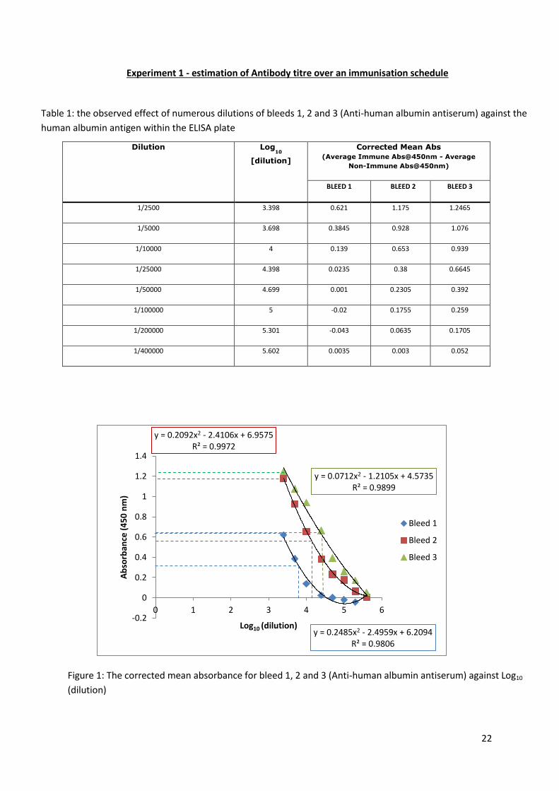
Experiment 1 - estimation of Antibody titre over an immunisation schedule

Table 1: the observed effect of numerous dilutions of bleeds 1, 2 and 3 (Anti-human albumin antiserum) against the

human albumin antigen within the ELISA plate

Dilution Log10

[dilution]

Corrected Mean Abs

(Average Immune Abs@450nm - Average

Non-Immune Abs@450nm)

BLEED 1 BLEED 2 BLEED 3

1/2500 3.398 0.621 1.175 1.2465

1/5000 3.698 0.3845 0.928 1.076

1/10000 4 0.139 0.653 0.939

1/25000 4.398 0.0235 0.38 0.6645

1/50000 4.699 0.001 0.2305 0.392

1/100000 5 -0.02 0.1755 0.259

1/200000 5.301 -0.043 0.0635 0.1705

1/400000 5.602 0.0035 0.003 0.052

Figure 1: The corrected mean absorbance for bleed 1, 2 and 3 (Anti-human albumin antiserum) against Log10

(dilution)

y = 0.2485x2 - 2.4959x + 6.2094 R² = 0.9806

y = 0.2092x2 - 2.4106x + 6.9575 R² = 0.9972

y = 0.0712x2 - 1.2105x + 4.5735 R² = 0.9899

-0.2

0

0.2

0.4

0.6

0.8

1

1.2

1.4

0 1 2 3 4 5 6

Ab

sorb

ance

(4

50

nm

)

Log10 (dilution)

Bleed 1

Bleed 2

Bleed 3

23

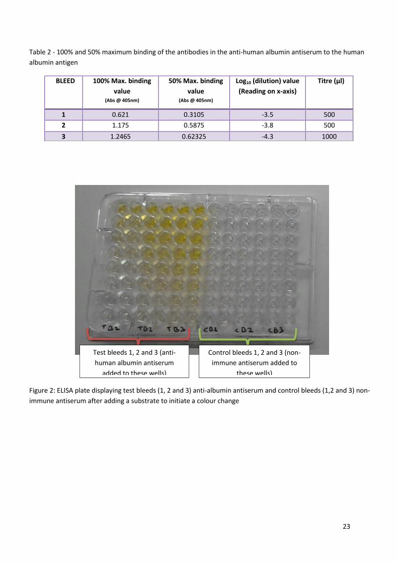
Table 2 - 100% and 50% maximum binding of the antibodies in the anti-human albumin antiserum to the human

albumin antigen

Figure 2: ELISA plate displaying test bleeds (1, 2 and 3) anti-albumin antiserum and control bleeds (1,2 and 3) non-

immune antiserum after adding a substrate to initiate a colour change

BLEED 100% Max. binding

value (Abs @ 405nm)

50% Max. binding

value (Abs @ 405nm)

Log10 (dilution) value

(Reading on x-axis)

Titre (μl)

1 0.621 0.3105 -3.5 500

2 1.175 0.5875 -3.8 500

3 1.2465 0.62325 -4.3 1000

Test bleeds 1, 2 and 3 (anti-

human albumin antiserum

added to these wells)

Control bleeds 1, 2 and 3 (non-

immune antiserum added to

these wells)

24

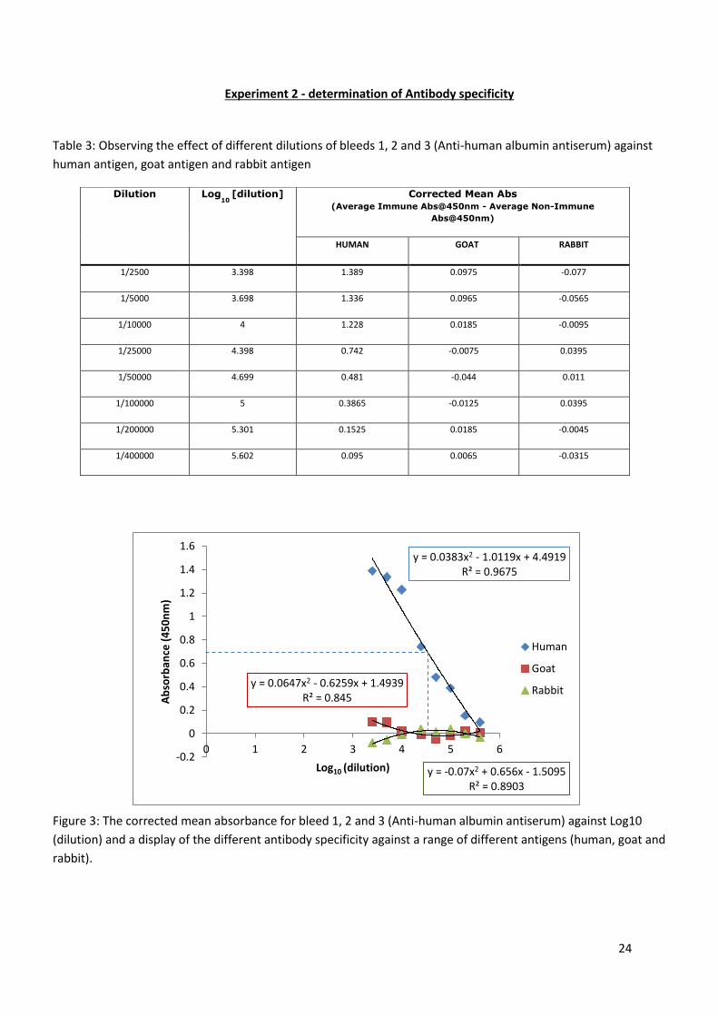
Experiment 2 - determination of Antibody specificity

Table 3: Observing the effect of different dilutions of bleeds 1, 2 and 3 (Anti-human albumin antiserum) against

human antigen, goat antigen and rabbit antigen

Figure 3: The corrected mean absorbance for bleed 1, 2 and 3 (Anti-human albumin antiserum) against Log10

(dilution) and a display of the different antibody specificity against a range of different antigens (human, goat and

rabbit).

Dilution Log10

[dilution] Corrected Mean Abs

(Average Immune Abs@450nm - Average Non-Immune

Abs@450nm)

HUMAN GOAT RABBIT

1/2500 3.398 1.389 0.0975 -0.077

1/5000 3.698 1.336 0.0965 -0.0565

1/10000 4 1.228 0.0185 -0.0095

1/25000 4.398 0.742 -0.0075 0.0395

1/50000 4.699 0.481 -0.044 0.011

1/100000 5 0.3865 -0.0125 0.0395

1/200000 5.301 0.1525 0.0185 -0.0045

1/400000 5.602 0.095 0.0065 -0.0315

y = 0.0383x2 - 1.0119x + 4.4919 R² = 0.9675

y = 0.0647x2 - 0.6259x + 1.4939 R² = 0.845

y = -0.07x2 + 0.656x - 1.5095 R² = 0.8903

-0.2

0

0.2

0.4

0.6

0.8

1

1.2

1.4

1.6

0 1 2 3 4 5 6

Ab

sorb

ance

(4

50

nm

)

Log10 (dilution)

Human

Goat

Rabbit

25

Table 4: Calculated data to determine the 100% and 50% maximum binding of the antibodies within anti-human

albumin antiserum to human antigen, goat antigen and rabbit antigen within the ELISA plates.

Figure 4: ELISA plate displaying test human, goat and rabbit antigen and control human, goat and rabbit albumin after

adding a substrate to initiate a colour change to show specificity of the antibody.

Reflection

From the results for experiment 1, bleed 1 has produced the least antibodies to target the antigen (human albumin). After

a 2nd immunisation the amount of antibody to antigen binding has doubled, proving the animal has since produced

memory B-cells for a quick response of future exposure to the antigen with a higher specificity of antibodies. Bleed 3 gave

the highest amount of antibody to antigen binding, but the increase wasn’t as sharp as what was seen in bleed 2, despite

a higher titre of bleed 3 binding antigen. This could be due to oversaturation of antibody within the wells as there is only a

limited amount of antigen that can be bound in the one area.

In experiment 2, the specificity of the antibody was almost exclusive to human albumin (figure 3). There is a slight

antibody to antigen interaction from the goat albumin at a low dilution (figure 3), but this and the signs of ab-ag binding

seen in the 1/25000, 1/50000 and 1/100000 of the rabbit, could both be due to an anomaly. Further testing would prove

if this is the case but for the most part the results gained from the goat and rabbit where non-specific to the anti-human

albumin antiserum (Table 3). The strong specificity of the antibody to the albumin is also clearly apparent in figure 4.

SPECIES 100% Max.

binding value (Abs @ 405nm)

50% Max.

binding value (Abs @ 405nm)

Log10 (dilution)

value (Reading on x-axis)

Titre (μl)

Human 1.389 0.6945 4.6 500

Goat 0.0975 0.0487 3.7 500

Rabbit 0.0395 0.0197 4.4 500

Test human, goat and rabbit

antigen (anti-human

albumin antiserum added to

these wells)

Control human, goat and

rabbit antigen (non-

immune antiserum added

to these wells)

26


Source: Genetics and Immunology

Experiment: Assessing the GMO status of a selected plant food

Portfolio Skills:


1. Correct use of automated pipettes 2. The use of positive and negative controls 3. Carrying out PCR 4. Carrying out agarose gel electrophoresis 5. Visualising results using gel

documentation devise

1. Use of PPE and aseptic technique 2. Time management 3. Following a protocol 4. Using a computer based data storage

system

Aim:

Use PCR to amplify DNA from test food sample and control samples (GMO-positive food and GMO-negative food)

Use electrophoresis to assess whether or not test food is GMO positive or negative.

Summary of evidence

Fresh corn was chosen as the plant food tested for genetic modification. The DNA of this test sample was extracted by

homogenisation using a pestle and mortar. The test DNA, plus positive and negative control plant DNA were then

prepared before being added to a thermal cycler which amplified the DNA by polymerase chain reaction (PCR). After

amplification of DNA the samples were added into wells of an agarose gel and electrophoresis was carried out to assess if

GMO primers had annealed to the sample. All lanes contained plant DNA so the lanes that contained plant primers (lanes

1, 3 and 5) should show bands at 500bp. Only the GMO positive DNA (lane 6) would bond to GMO primers at 200bp,

therefore acting as a positive control. The non-GMO DNA (lane 2) did not bond to GMO primers therefore acting as the

negative control. The corn (test plant food) did not generate a 200bp band with GMO primers therefore making it GMO

negative.

Result

The chosen plant food (fresh corn) was GMO negative


27

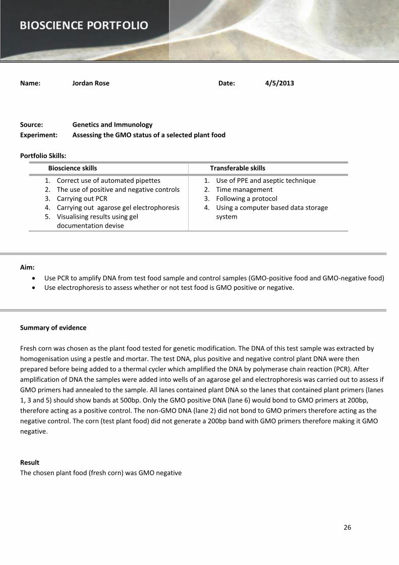
Portfolio Evidence

Figure 1: A visualisation of the gel electrophoresis that determines the GMO content of the test substances, including

positive and negative controls. Lane 1: non-GMO food with plant primers, Lane 2: non-GMO food with GMO primers,

Lane 3: Test food with plant primers, Lane 4: Test food with GMO primers, Lane 5: GMO positive template with plant

primers, Lane 6: GMO positive template with GMO primers, Lane 7: PCR molecular weight (MW) Ruler.

Table 1; Results of the gel electrophoresis. When a sample binds with plant primers it forms a 500bp band. When a

sample binds with GMO primers it forms a 200bp band.

Lane Sample Bands (yes/no)? Band sizes (bp)

1 Non-GMO food control with plant primers Yes 500

2 Non-GMO food control with GMO primers No 0

3 Test food control with plant primers Yes 500

4 Test food control with GMO primers No 0

5 GMO positive control with plant primers Yes 500

6 GMO positive control with GMO primers Yes 200

7 PCR Molecular Weight Ruler Yes 1000, 700, 500, 200, 100

1 2 3 4 5 6 7

1 2 3 4 5 6 7

28

Reflection

The result of the experiment was that the test food was GMO-negative, therefore leading to the assumption that the corn

was not genetically modified. To conclude that this was an accurate result for this corn crop a further study that looked at

more samples of the same corn crop would be acceptable.

There is a potential risk that my result was only showing as GMO-negative due to the potential acidic pH of the fresh corn

altering or denaturing the DNA when it was released from the cells, therefore leaving none to amplify. This problem

would not occur if the food that was tested was processed. Assessing the pH of the fresher foods would be appropriate

for future tests in order to rectify this potential problem with the procedure.

Perhaps another improvement could be using a different technique to extract the DNA from cells. The use of ultrasonic

lysis (soft sonification for DNA extraction) would be appropriate to make sure DNA is actually extracted as this could have

also been a reason for the negative result. Using the pestle and mortar is cheap, quick and easy to do but could have

been a potential reason why there was potentially no DNA extracted.

In regards to the techniques I have carried out, both are essential in an analytical laboratory setting. Using electrophoresis

to separate proteins and DNA according to size is a good way to study them and find out which proteins are in the cells

according to an appropriate MW ruler. PCR is an expensive technique but it is useful to use when there is a small sample

available. This means the DNA can be amplified so that multiple tests can be run using the same original sample.

29


Source: Clinical Biochemistry

Experiment: Screening for inborn errors in metabolism

Portfolio Skills:


1. The use of Thin Layer Chromatography 2. The use of positive and negative controls 3. Careful handling of human samples

1. Use of PPE and aseptic technique 2. Using initiative and understanding to choose

appropriate methods/tests 3. Tabulating results

Aim

To diagnose any errors in the metabolism of four neonatal urine samples.

Use thin layer chromatography (TLC) to identify the amino acids present in samples (A to D).

Ferric chloride test is carried out to detect phenols in the samples.

Use TLC to detect carbohydrates in the samples which tested negative for amino acids.

Specific tests should be carried out to identify the exact amino acids and carbohydrates present in the samples.

Summary of evidence

Urine sample A – From a neonate whose pregnancy and delivery were normal and it’s remained healthy

Urine sample B – From a mentally retarded patient

Urine sample C and D – From neonates failing to thrive.

Thin layer chromatography (TLC) was carried out on samples A to D to find the RF values and connect them to specific

amino acids. Once the results for the TLC are finalised, specific tests can be run to either conclude what amino acids are

present in the samples, and which can be ruled out. Samples A and B tested positive for amino acids, and sample C and D

tested negative, therefore they will be tested for carbohydrates.

A preliminary test for detecting inborn errors of metabolism can be carried out using the ferric chloride test. This is

achieved by noting the colour change of samples when 10% ferric chloride (FeCl3) is added drop-by-drop.

TLC with the standard sugars can be run next to the samples. Again the RF values are used to figure out which

carbohydrates have been found in the samples. More specific tests can be run to assess which carbohydrates are present

in the samples and which can be ruled out.

Conclusive diagnosis results

Sample A – Maple syrup urine disease

Sample B – Histidinemia

Sample C – Lactic acidosis (galactose present in urine)

Sample D – Essential fructosuria (fructose present in urine)


30

Portfolio evidence

Amino Acid Thin Layer Chromatography (TLC)

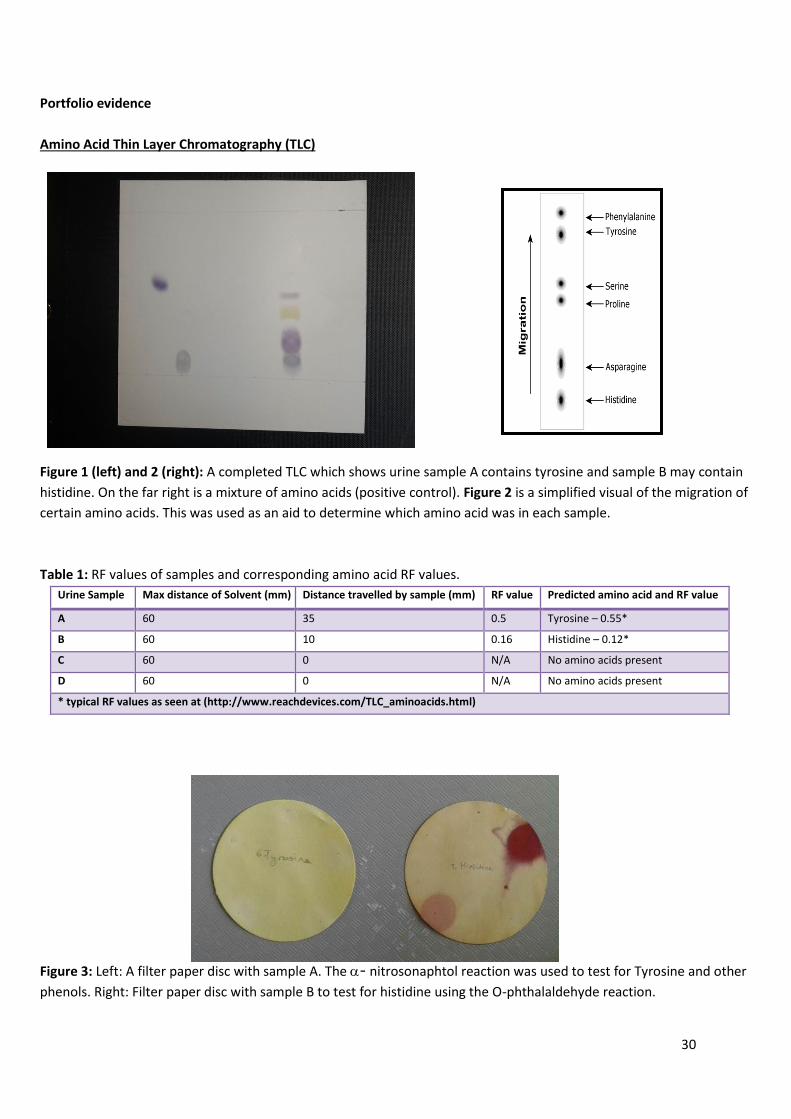
Figure 1 (left) and 2 (right): A completed TLC which shows urine sample A contains tyrosine and sample B may contain

histidine. On the far right is a mixture of amino acids (positive control). Figure 2 is a simplified visual of the migration of

certain amino acids. This was used as an aid to determine which amino acid was in each sample.

Table 1: RF values of samples and corresponding amino acid RF values.

Urine Sample Max distance of Solvent (mm) Distance travelled by sample (mm) RF value Predicted amino acid and RF value

A 60 35 0.5 Tyrosine – 0.55*

B 60 10 0.16 Histidine – 0.12*

C 60 0 N/A No amino acids present

D 60 0 N/A No amino acids present

* typical RF values as seen at (http://www.reachdevices.com/TLC_aminoacids.html)

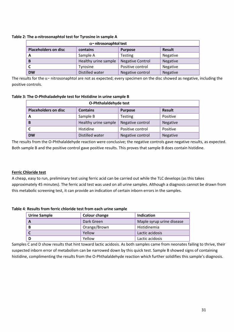
Figure 3: Left: A filter paper disc with sample A. The - nitrosonaphtol reaction was used to test for Tyrosine and other

phenols. Right: Filter paper disc with sample B to test for histidine using the O-phthalaldehyde reaction.

31

Table 2: The a-nitrosonaphtol test for Tyrosine in sample A

- nitrosonaphtol test

Placeholders on disc contains Purpose Result

A Sample A Testing Negative

B Healthy urine sample Negative Control Negative

C Tyrosine Positive control Negative

DW Distilled water Negative control Negative

The results for the - nitrosonaphtol are not as expected; every specimen on the disc showed as negative, including the

positive controls.

Table 3: The O-Phthaladehyde test for Histidine in urine sample B

O-Phthalaldehyde test

Placeholders on disc Contains Purpose Result

A Sample B Testing Positive

B Healthy urine sample Negative control Negative

C Histidine Positive control Positive

DW Distilled water Negative control Negative

The results from the O-Phthalaldehyde reaction were conclusive; the negative controls gave negative results, as expected.

Both sample B and the positive control gave positive results. This proves that sample B does contain histidine.

Ferric Chloride test

A cheap, easy to run, preliminary test using ferric acid can be carried out while the TLC develops (as this takes

approximately 45 minutes). The ferric acid test was used on all urine samples. Although a diagnosis cannot be drawn from

this metabolic screening test, it can provide an indication of certain inborn errors in the samples.

Table 4: Results from ferric chloride test from each urine sample

Urine Sample Colour change Indication

A Dark Green Maple syrup urine disease

B Orange/Brown Histidinemia

C Yellow Lactic acidosis

D Yellow Lactic acidosis

Samples C and D show results that hint toward lactic acidosis. As both samples came from neonates failing to thrive, their

suspected inborn error of metabolism can be narrowed down by this quick test. Sample B showed signs of containing

histidine, complimenting the results from the O-Phthalaldehyde reaction which further solidifies this sample’s diagnosis.

32

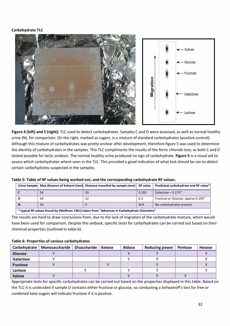
Carbohydrate TLC

Figure 4 (left) and 5 (right): TLC used to detect carbohydrates. Samples C and D were assessed, as well as normal healthy

urine (N), for comparison. On the right, marked as sugars, is a mixture of standard carbohydrates (positive control).

Although this mixture of carbohydrates was pretty unclear after development, therefore figure 5 was used to determine

the identity of carbohydrates in the samples. This TLC compliments the results of the ferric chloride test; as both C and D

tested possible for lactic acidosis. The normal healthy urine produced no sign of carbohydrate. Figure 5 is a visual aid to

assess which carbohydrates where seen in the TLC. This provided a good indication of what test should be ran to detect

certain carbohydrates suspected in the samples.

Table 5: Table of RF values being worked out, and the corresponding carbohydrate RF values.

Urine Sample Max distance of Solvent (mm) Distance travelled by sample (mm) RF value Predicted carbohydrate and RF value*

C 54 10 0.185 Galactose – 0.175*

D 54 12 0.2 Fructose or Glucose- approx 0.195*

N 54 0 N/A No carbohydrates present

* typical RF values found by (Wolfrom 1961) taken from “Advances in Carbohydrate Chemistry”

The results are hard to draw conclusions from, due to the lack of migration of the carbohydrate mixture, which would

have been used for comparison. Despite this setback, specific tests for carbohydrates can be carried out based on their

chemical properties (outlined in table 6).

Table 6: Properties of various carbohydrates

Carbohydrate Monosaccharide Disaccharide Ketose Aldose Reducing power Pentose Hexose

Glucose Y Y Y Y

Galactose Y Y Y Y

Fructose Y Y Y Y

Lactose Y Y Y Y

Xylose Y Y Y Y

Appropriate tests for specific carbohydrates can be carried out based on the properties displayed in this table. Based on

the TLC it is undecided if sample D contains either fructose or glucose, so conducting a Seliwanoff’s test for free or

combined keto-sugars will indicate fructose if it is positive.

33

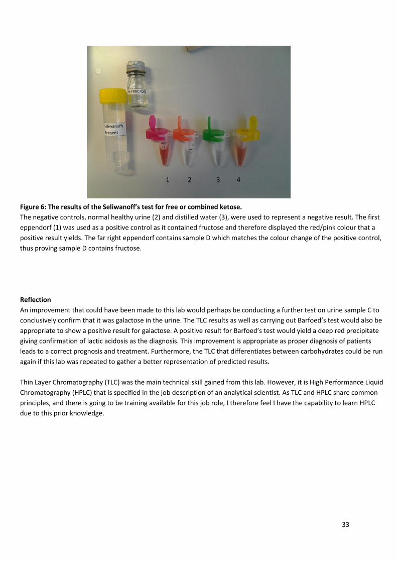
Figure 6: The results of the Seliwanoff’s test for free or combined ketose.

The negative controls, normal healthy urine (2) and distilled water (3), were used to represent a negative result. The first

eppendorf (1) was used as a positive control as it contained fructose and therefore displayed the red/pink colour that a

positive result yields. The far right eppendorf contains sample D which matches the colour change of the positive control,

thus proving sample D contains fructose.

Reflection

An improvement that could have been made to this lab would perhaps be conducting a further test on urine sample C to

conclusively confirm that it was galactose in the urine. The TLC results as well as carrying out Barfoed’s test would also be

appropriate to show a positive result for galactose. A positive result for Barfoed’s test would yield a deep red precipitate

giving confirmation of lactic acidosis as the diagnosis. This improvement is appropriate as proper diagnosis of patients

leads to a correct prognosis and treatment. Furthermore, the TLC that differentiates between carbohydrates could be run

again if this lab was repeated to gather a better representation of predicted results.

Thin Layer Chromatography (TLC) was the main technical skill gained from this lab. However, it is High Performance Liquid

Chromatography (HPLC) that is specified in the job description of an analytical scientist. As TLC and HPLC share common

principles, and there is going to be training available for this job role, I therefore feel I have the capability to learn HPLC

due to this prior knowledge.

1 2 3 4

34


Source: DNA and Antibody techniques

Experiment: precipitation techniques in agar (Immunodiffusion)

Portfolio Skills:


1. Carrying out single and double immunodiffusion assays

2. Making serial dilutions 3. Correct use of an automated pipette

1. Use of PPE and aseptic technique 2. Following a protocol 3. Data Analysis 4. Displaying data graphically

Aims:

Preform a double immunodiffusion assay and record the distance the line of precipitation has travelled to determine the titre of an anti-human albumen antiserum.

Preform a single immunodiffusion assay and measure the diameter of each ring (mm) to construct a standard calibration graph. Then calculation the concentration of amylase in the sample of saliva.

Summary of evidence

In a double radial immunodiffusion (Serological Ouchterlony test), the antigen (Ag) and antibody (Ab) diffuse through the

gel to reach each other and form an immune complex. This Ag-Ab immune complex is made of a lattice which forms only

when Ag and Abs are at an optimal ratio, also known as the zone of equivalence. Only at this point can they form a

precipitate and be visualised as a white line in the gel. This technique is used to check antiserum for the presence of Abs

that will bond to a particular Ag and to determine at what titre it will still be able to form an immune complex.

The single radial immunodiffusion (mancini test) is a technique used to determine the quantity of an antigen (Ag). In the

case of this experiment, the Ag was the enzyme amylase which was able to interact with the anti-human amylase

antibody (Ab) that was suspended in the gel. As the Ag travelled it left a ring of clearance caused by the Remazol Brilliant

Blue dye in the gel being lightened by Ag and Ab interaction. This technique is useful in determining how much amylase is

in the saliva samples used as it shows the clear zones well against the blue background. The results concluded that the

average 1/5 dilution of saliva contained 2mg/ml of amylase, 1/10 and 1/20 both contained 0.5mg/ml of amylase. Further

repeats of the experiment or the use of a range of results from the entire lab class would have made these average

results a lot more reliable.


35

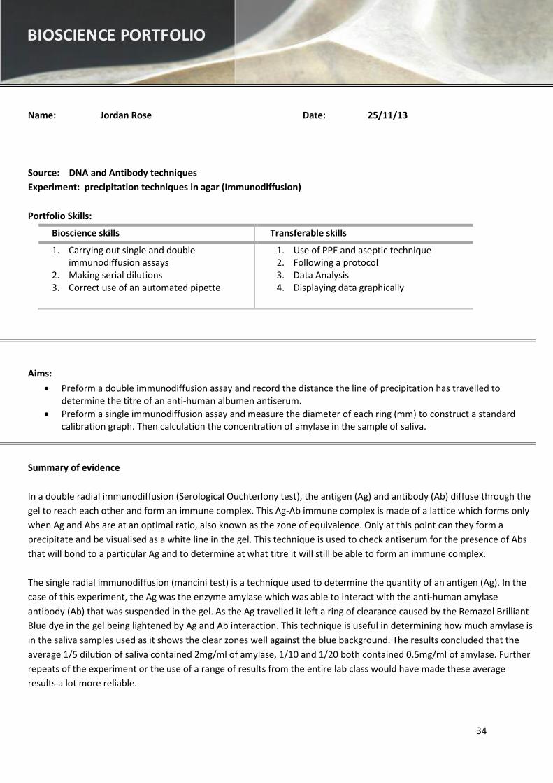
Portfolio evidence

Experiment 1 : Double Immunodiffusion Assay

Figure 1. Double radial immunodiffusion (Serological Ouchterlony). The bottom wells contain a range of dilutions of the

antiserum. The well labelled neat contains only Anti-albumin Antibody (15µl). After this, the 1/2 is made up of 15µl Anti-

albumin Antibody and 15µl of PBS (diluent) and so on to make up the 1/4, 1/8, 1/16 and 1/32 dilutions via serial dilution.

Each of the top wells contains 1mg/ml Albumen (Antigen).

Table 1: the distance travelled by the Anti-Albumin antibody to form an immunoprecipitate with an antigen. An

immunoprecipitate was formed with the Neat, 1/2 , 1/4 and 1/8 dilutions of the antibody. In all further dilutions there

were not enough antibodies available to form lattices and no visual line of precipitation could be measured

Distance migrated by the Precipitate

Ab

Dilution

Distance migrated (mm) (Relative to ANTIBODY well)

Distance migrated (mm) (Relative to ANTIGEN well)

Neat 7 7

1/2 6 8

1/4 5 9

1/8 No precipitate No precipitate

1/16 No precipitate No precipitate

1/32 No Precipitate No precipitate

Neat 1/2 1/4 1/8 1/16 1/32

1mg/ml Albumin

(Antigen)

Anti-albumin

various dilutions

(Antibody)

36

Experiment 2: Single Radial Immunodiffusion Assay

Figure 2: A Mancini (single radial immundiffusion) test to determine the amylase content of human saliva. The gel itself

is made up of 1% agar /0.6 % anti-human amylase antibody/0.25 % Remazol Brilliant Blue. Over time, the amylase bonds

with the antibodies and the blue colour fades, leaving a clearance zone. This clearance can be measured to determine

how much amylase is in each saliva dilution. The top 6 wells contain a dilution of the enzyme amylase. (1) Contains

10mg/ml amylase solution, (2) contains 5mg/ml amylase solution, (3) contains 2mg/ml amylase solution, (4) contains

1mg/ml amylase solution, (5) contains 0,5mg/ml amylase solution, and (6) contains 0.25mg/ml amylase solution. The

bottom row of wells contains saliva sample 1 (dilutions of 1/5, 1/10 and 1/20) and saliva sample 2 (repeat dilutions).

Table 2: The standard concentration of amylase in each well and the ring diameter, plus the diameter squared left in

the gel by the enzyme. This information can be used later for comparison with the dilutions of saliva placed into the wells

(Shown in figure 2). It’s clear to see that the more amylase present in the well the greater the interaction with the anti-

human antibody, thus the larger the ring diameter.

Amylase Concentration (mg/ml)

Ring Diameter (mm) [Ring Diameter (mm)]2

0.25 12 144

0.5 14 196

1 15 225

2 16 256

5 17 289

10 18 324

1/5 1/5 1/10 1/20 1/10 Saliva sample 1 (1) (2) (3) (4) (5)

(1) (2) (3) (4) (5) (6)

Saliva Sample 1 Saliva Sample 2

Repeat

1/5 1/10 1/10 1/20 1/20 1/5

37

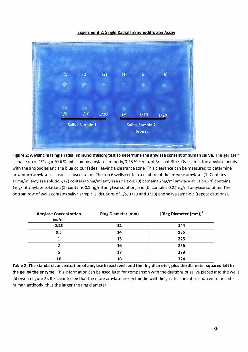
Figure 3: Ring diameter of various amylase standards with varying concentration. A is amylase standard at 10mg/ml

with a ring diameter of 18mm (324mm2), B is amylase standard at 5mg/ml with a ring diameter of 17mm (289mm2), C is

amylase standard at 2mg/ml with a ring diameter of 16mm (256mm2), D is amylase standard at 1mg/ml with a ring

diameter of 15mm (225mm2), E is amylase standard at 0.5mg/ml with a ring diameter of 14mm (196mm2), and F is

amylase standard at 0.25mg/ml with a ring diameter of 12mm (144mm2).

Table 3: The ring diameter of the saliva samples 1 and 2 and their average ring diameter. These results have been

compared with the results gained from our standard ring diameter of amylase (table 2) to gain the amount of amylase

thought to be in the saliva samples. Upon gaining an average it is evident that 1/5 dilution of saliva is equal to 2mg/ml of

amylase, 1/10 dilution of saliva is equal to 0.5mg/ml of amylase, and 1/20 of saliva is equal to 0.5mg/ml of amylase.

Saliva Dilutions Ring Diameter (mm) Average

Diameter

Sample Amylase

Conc (mg/ml)

Final Amylase

Conc (mg/ml) Rep 1 Rep 2

1 in 5 18 15 16.5 20 2

1 in 10 16 13 14.5 20 0.5

1 in 20 15 12 13.5 20 0.5

38

Reflection

The double immunodiffusion assay is a technique used to assess antiserum for the presence of antibodies that will bond

to a particular antigen. This will aid in determining at what titre the antibodies will have to be in order to form a visual

immune complex. Perhaps repeating this technique or viewing the whole lab class results would be worthwhile in order

to determine if my results are truly reliable or not.

For the single radial immunodiffusion assay, the average of the two repeats tests shows that the saliva sampled contains

2mg/ml of amylase. Despite one repeat of the experiment showing a lower concentration of amylase and the other

showing a higher concentration of amylase, this result is good as it proves that amylase is found within the human mouth.

As with the last technique, more repeats could be carried out as the results were wide spread and therefore gave an

average that was lower than expected. Repeating the test or looking at other class results would help to better

determine the correct amount of amylase in the saliva sample and check the reliability of my results.

39


Source: Pathophysiology and pharmacology of cells and tissues

Experiment: Sensitisation of smooth muscle tissue

Portfolio Skills:


1. Set up and use of a gut bath 2. Safe handling of animal tissue 3. Safe handling of various chemicals

1. Use of PPE and aseptic technique 2. Following a protocol 3. Use of Minitab (Statistical analysis) 4. Data analysis 5. Displaying data graphically

Aim:

To understand the response of non-sensitized and sensitized guinea pig ileum to egg albumen, bovine serum albumen, the agonists carbachol and histamine, and how the antagonist mepyramine affects response.

To determine the identity of the chemical that is released from sensitized mast cells.

To use Minitab to conduct statistical analysis of results.

Summary of evidence

In this lab, egg albumen is used as an example of a food allergen. The guinea pigs were kept in a clean environment

therefore making this protein foreign and therefore a threat to the health of the animal by their immune system.

Immunoglobulin E antibodies are produced when egg albumen is introduced to the tissue, and these antibodies attach to

high affinity FcepsilonRI (FcεRI) receptors on mast cells. A second exposure to egg albumen (figure 3) will result in the

allergen binding with the IgE antibodies, which would activate a coupled receptor. This causes mast cell degranulation,

and the release of many substances including preformed mediators. This is known as type I hypersensitivity and this

causes the smooth muscle of the guinea pig ileum to contract due to histamine being released from within preformed

mediators.

Mepyramine, a first generation antihistamine, acts as an antagonist and stops the histamine having this effect and is

therefore assessed (Figure 1,2 and 3). Carbachol, a cholinomimetic drug that activates the muscarinic acetylcholine

receptor, M3, is also looked at and compared to histamine. BSA was used as a control as it is not meant to cause any

contraction of smooth muscle.

Result

Histamine is the chemical assumed to cause smooth muscle contraction in this lab.


40

Portfolio Evidence

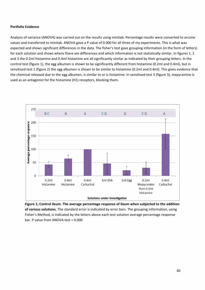
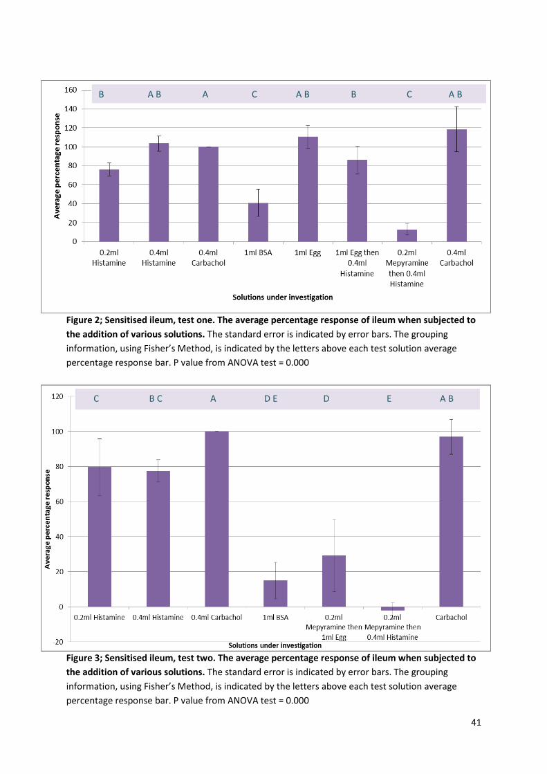
Analysis of variance (ANOVA) was carried out on the results using minitab. Percentage results were converted to arcsine

values and transferred to minitab. ANOVA gave a P value of 0.000 for all three of my experiments. This is what was

expected and shows significant differences in the data. The fisher’s test gave grouping information (in the form of letters)

for each solution and shows where there are differences and which information is not statistically similar. In figures 1, 2

and 3 the 0.2ml histamine and 0.4ml histamine are all significantly similar as indicated by their grouping letters. In the

control test (figure 1), the egg albumen is shown to be significantly different from histamine (0.2ml and 0.4ml), but in

sensitised test 1 (figure 2) the egg albumen is shown to be similar to histamine (0.2ml and 0.4ml). This gives evidence that

the chemical released due to the egg albumen, is similar to or is histamine. In sensitised test 3 (figure 3), mepyramine is

used as an antagonist for the histamine (H1) receptors, blocking them.

Figure 1; Control ileum. The average percentage response of ileum when subjected to the addition

of various solutions. The standard error is indicated by error bars. The grouping information, using

Fisher’s Method, is indicated by the letters above each test solution average percentage response

bar. P value from ANOVA test = 0.000

B C B A C D D C D A

41

Figure 2; Sensitised ileum, test one. The average percentage response of ileum when subjected to

the addition of various solutions. The standard error is indicated by error bars. The grouping

information, using Fisher’s Method, is indicated by the letters above each test solution average

percentage response bar. P value from ANOVA test = 0.000

Figure 3; Sensitised ileum, test two. The average percentage response of ileum when subjected to

the addition of various solutions. The standard error is indicated by error bars. The grouping

information, using Fisher’s Method, is indicated by the letters above each test solution average

percentage response bar. P value from ANOVA test = 0.000

B A B A C A B B C A B

C B C A D E D E A B

42

Reflection

The results gained from all tests, most notably those from sensitised test 1 (figure 2) and sensitised test 2 (figure

3), seem to conclusively point toward the chemical realised from the mast cells that’s responsible for the smooth

muscle contraction is histamine. My research did however show that mast cells degranulation releases an

assortment of chemicals into the extracellular environment. Separation of these constituents using high-

performance liquid chromatography (HPLC) would be appropriate for further investigation and also make the

evidence that histamine is responsible a lot stronger.

During this experiment, the BSA used was thought to be contaminated therefore showing unexpected results. If

this experiment was repeated in the future, the batch of BSA to be used should be brand new and sterile,

therefore giving a control that does not interfere with results.

43


Source: Various modules

Skill: Scientific poster presentation

Portfolio Skills:


1. Understand, interpret and explain complex scientific concepts

2. Research, analyse and critique journals

1. Using Microsoft PowerPoint 2. Confidently and clearly presenting work 3. Learning from feedback for future improvement

Aim:

Research and construct a poster that summarises the main concepts and areas of research addressing a particular poster title.

The use of figures, flowcharts and concise information will make the topic accessible and easy to follow.

Presenting the poster to an audience will expand on the information given on the posters, displaying a wider knowledge of the subject area.

Evidence Review

Summary of evidence

A scientific poster is an effective way to convey a particular scientific concept. It should be accessible to other researchers

in that field as well as drawing an interest to a more general audience. A poster should be a concise, eye-catching and

thought-provoking way of showing your research, and/or results, which should prompt others to want to further

understand the topic. The use of flowcharts, pictures, diagrams, tables and other figures breaks up the written segments

of the poster and makes the information easier to digest. Giving a presentation of your work in this way enables you to

add to the information already there and influence the audience to ask questions, making the poster more interactive and

memorable.


44

Portfolio evidence

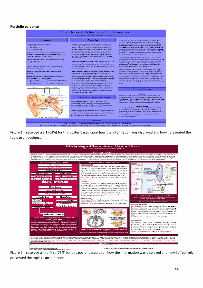
Figure 1; I received a 2.1 (64%) for this poster based upon how the information was displayed and how I presented the

topic to an audience.

Figure 2; I received a mid-first (75%) for this poster based upon how the information was displayed and how I effectively

presented the topic to an audience.

45

Reflection

Of my two posters, I feel that Figure 2 is the better of the pair. This is due to the fact that Figure 1 didn’t have a layout or

colour scheme that was as aesthetically pleasing as figure 2. Although a lot of research was put into this poster, there are

too many words bombarding the reader causing a loss of focus and overall disinterest in reading it all. Even though there

is a picture, the choice of including this particular picture didn’t add any new information to poster as it just reiterated

what was written. An improvement would be changing the colour and layout to something that is more attractive to the

viewer and cutting a lot of unnecessary words so the poster feels less like a book and more attractive to the eye. Bullet

points, flow charts, or diagrams would help to facilitate this.

Figure 2 has a layout and colour scheme which was more clean and professional. There was a lot of information but it was

given in a number of different ways, giving the poster more of a flow and making it easier to read overall. Although there

are still large chunks of written information, it is peppered throughout the poster, rather than bombarding the audience

with too much. When this poster was presented, all the information could be related in some way to every picture on

display. This allowed the audience to follow the information and find an interest in the topic as a whole compared to the

first poster (figure 1). The improvement of my grade also reflects how this was a better poster/presentation overall and

although I am happy with the outcome, further improvements such as expanding on novel research based on treatment

for instance would make the poster more distinguished and helpful for the reader in the long term.

Updated portfolio skills october 2015

Documents

Transcript of Updated portfolio skills october 2015