University of Groningen Multichannel EEG Visualization ...
31
University of Groningen Multichannel EEG Visualization Caat, Michael ten IMPORTANT NOTE: You are advised to consult the publisher's version (publisher's PDF) if you wish to cite from it. Please check the document version below. Document Version Publisher's PDF, also known as Version of record Publication date: 2008 Link to publication in University of Groningen/UMCG research database Citation for published version (APA): Caat, M. T. (2008). Multichannel EEG Visualization. s.n. Copyright Other than for strictly personal use, it is not permitted to download or to forward/distribute the text or part of it without the consent of the author(s) and/or copyright holder(s), unless the work is under an open content license (like Creative Commons). The publication may also be distributed here under the terms of Article 25fa of the Dutch Copyright Act, indicated by the “Taverne” license. More information can be found on the University of Groningen website: https://www.rug.nl/library/open-access/self-archiving-pure/taverne- amendment. Take-down policy If you believe that this document breaches copyright please contact us providing details, and we will remove access to the work immediately and investigate your claim. Downloaded from the University of Groningen/UMCG research database (Pure): http://www.rug.nl/research/portal. For technical reasons the number of authors shown on this cover page is limited to 10 maximum. Download date: 28-02-2022
Transcript of University of Groningen Multichannel EEG Visualization ...

University of Groningen
Multichannel EEG VisualizationCaat, Michael ten
IMPORTANT NOTE: You are advised to consult the publisher's version (publisher's PDF) if you wish to cite fromit. Please check the document version below.
Document VersionPublisher's PDF, also known as Version of record
Publication date:2008
Link to publication in University of Groningen/UMCG research database
Citation for published version (APA):Caat, M. T. (2008). Multichannel EEG Visualization. s.n.
CopyrightOther than for strictly personal use, it is not permitted to download or to forward/distribute the text or part of it without the consent of theauthor(s) and/or copyright holder(s), unless the work is under an open content license (like Creative Commons).
The publication may also be distributed here under the terms of Article 25fa of the Dutch Copyright Act, indicated by the “Taverne” license.More information can be found on the University of Groningen website: https://www.rug.nl/library/open-access/self-archiving-pure/taverne-amendment.
Take-down policyIf you believe that this document breaches copyright please contact us providing details, and we will remove access to the work immediatelyand investigate your claim.
Downloaded from the University of Groningen/UMCG research database (Pure): http://www.rug.nl/research/portal. For technical reasons thenumber of authors shown on this cover page is limited to 10 maximum.
Download date: 28-02-2022
Chapter 3
Data-Driven Visualization of MultichannelEEG Coherence with Functional Units
Abstract
Synchronous electrical activity in different brain regions is generally assumed to implyfunctional relationships between these regions. A measure for this synchrony is electroen-cephalography (EEG) coherence, computed between pairs of signalsas a function of fre-quency. A typical data-driven visualization of electroencephalography(EEG) coherenceis a graph layout, with vertices representing electrodes and edges representing significantcoherences between electrode signals. A drawback of this layout is its visual clutter formultichannel EEG. To reduce clutter, we define a functional unit (FU) as adata-driven re-gion of interest (ROI). An FU is a spatially connected set of electrodes recording pairwisesignificantly coherent signals, represented in the coherence graph bya spatially connectedclique. We present three methods to detect FUs. One is a maximal clique based (MCB)method (time complexity O(3n/3), with n the number of vertices). Another is a more effi-cient watershed based (WB) method (time complexity O(n2 logn)). To reduce the potentialover-segmentation of the WB method, the improved watershed based (IWB) method (timecomplexity O(n2 logn)) merges basins representing FUs during the segmentation if they arespatially connected and if their union is a clique. The WB and IWB method both are up to afactor of 100,000 times faster than the MCB method for a typical multichannel setting with128 EEG channels, thus making interactive visualization of multichannel EEGcoherencepossible. Results show that, considering the MCB method as the gold standard, the differ-ence between IWB and MCB FU maps is smaller than between WB and MCB FU maps. Wealso introduce two novel group maps for data-driven group analysis as extensions of the IWBmethod. First, the group mean coherence map preserves dominant features from a collec-tion of individual FU maps. Second, the group FU size map visualizes the average FU sizeper electrode across a collection of individual FU maps. Finally, we employan extensivecase study to evaluate the IWB FU map and the two new group maps for data-driven groupanalysis. Results, in accordance with conventional findings, indicate differences in EEGcoherence between younger and older adults. However, they also suggest that an initialselection of hypothesis-driven ROIs could be extended with additional data-driven ROIs.
40 3.1 Introduction
3.1 Introduction
Electroencephalography (EEG) is a method to measure the electrical activity of the brain usingelectrodes attached to the scalp at multiple locations. Synchronous electrical activity in differentbrain regions is generally assumed to imply functional relationships between these regions. Ameasure for this synchrony is EEG coherence, calculated between pairs of electrode signals as afunction of frequency (Hallidayet al.1995, Mauritset al.2006).
Related studies of functional brain connectivity use other noninvasive neuroimaging tech-niques, including magnetoencephalography (MEG) (Bosboomet al. 2006, Chenet al. 2003,Srinivasanet al.1999) and functional magnetic resonance imaging (fMRI) (Achardet al.2006,Cordeset al.2002, Salvadoret al.2005b, Salvadoret al.2005a). A typical visualization of EEG,MEG, and fMRI coherence, is a two-dimensional graph layout. Vertices represent electrodes,superconducting quantum interference devices (SQUIDS), or fMRI regions of interest (ROIs),respectively. Edges represent significant coherences between electrode signals, SQUID signals,or fMRI-ROI time series, respectively. Vertices are commonly visualized as dots and edges aslines. For multichannel EEG (e.g., (Kaminski et al.1997, Steinet al.1999)), MEG (e.g., (Chenet al.2003, Srinivasanet al.1999)), and fMRI (e.g., (Achardet al.2006, Salvadoret al.2005b)),this layout may suffer from a large number of overlapping edges, resulting in a cluttered visual-ization.
In the case of EEG, the reorganization of vertex positions (Fruchterman and Reingold 1991)to reduce clutter is not appropriate, because the electrodes have meaningful positions. Other so-lutions reorganize edges or vary visual attributes of the edges (Wonget al. 2003, Hermanet al.2000), but do not reduce the number of edges. Several methodsdivide EEG electrodes (Sarntheinet al.1998, Gladwinet al.2006), MEG SQUIDS (Bosboomet al.2006), or fMRI voxels (Salvadoret al.2005a) into disjoint hypothesis-driven ROIs and study coherences within or between ROIs.Other methods set out ROIs representing EEG electrodes (Kaminski et al. 1997, Franaszczuket al. 1994), MEG SQUIDS (Srinivasanet al. 1999), or fMRI-ROIs (Achardet al. 2006) alongrows and columns, thus obtaining a square contingency table. By arranging ROIs along rows andcolumns of a matrix, the spatial relations are lost.
Visualization of multichannel EEG (at least 64 electrodes)is not always managed well (tenCaatet al. 2005, ten Caatet al. 2007c, ten Caatet al. 2007d). Researchers often employ ahypothesis-driven definition of certain ROIs in which all electrodes are assumed to record similarsignals because of volume conduction effects (Lachauxet al. 1999). As an alternative for thehypothesis-driven approach, we introduce three methods todetect data-driven ROIs referred toas functional units (FUs) (ten Caatet al.2007d). An FU is represented in the coherence graphby a spatially connected clique. A clique is a vertex set in which every two-element subset isconnected by an edge. A cliqueC is maximalwhen it is not contained in any larger clique(‘larger’ meaning having more vertices). Within one FU, each pair of vertices represents twosignificantly coherent electrode signals. In any group of vertices other than a clique, there aretwo vertices representing two electrode signals which are not significantly coherent. Becauselarger ROIs are assumed to correspond to stronger source signals, larger FUs are consideredto be more interesting. Therefore, we focus on maximal cliques, with vertex sets as large aspossible.
Data-Driven Visualization of Multichannel EEG Coherence with FunctionalUnits 41
Our first FU detection method is a maximal clique based (MCB) method (ten Caatet al.2007d). Our second method is a watershed based (WB) method that detects spatially con-nected cliques in a greedy way (ten Caatet al. 2007e). However, it suffers from potentialover-segmentation problems. A third method is an improved watershed based (IWB) methodfor FU detection. It merges FUs if they are spatially connected and if their union is a clique, thusreducing over-segmentation obtained with the WB method. A functional unit map shows the FUdistribution for individual datasets. Each FU is a collection of Voronoi cells with identical grayvalue, with different gray values for adjacent FUs. FUs are connected by a line if the averagecoherence between FUs is significant.
In addition to individual dataset analysis, we introduce two new group maps for data-drivengroup analysis of multichannel EEG coherence as extensionsof the IWB method. They serveas a data-driven alternative for the common hypothesis-driven selection of coherences for groupanalysis (Mauritset al.2006, Gladwinet al.2006, Knyazevaet al.2006). First, the group meancoherence map preserves dominant features from a collection of individual FU maps. Second, thegroup FU size map visualizes the average FU size per electrode across a collection of individualFU maps. Results are reported for an extensive case study.
3.2 EEG Coherence
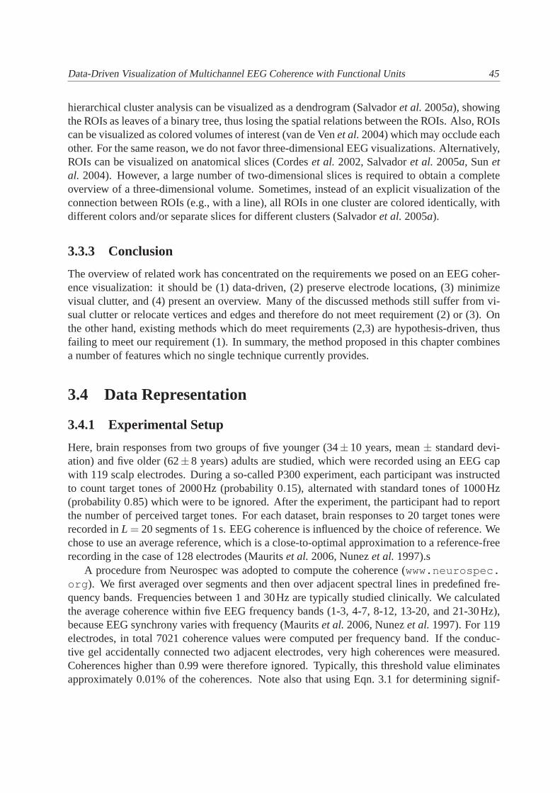
EEG can be recorded using currently up to 512 electrodes, labeled uniquely by a combinationof letters and digits (e.g., F3, Cz, P4, as in Fig. 3.1, right).A conductive gel is applied betweenskin and electrodes to reduce impedance. The electrical potential is measured at all electrodessimultaneously. The measured signals are amplified, resulting in one recording channel for everyelectrode. If there are many electrodes, the term ‘multichannel’ or ‘high-density’ EEG is used.As a result of volume conduction (Lachauxet al.1999), multiple electrodes can record a signalfrom a single source in the brain. Therefore, nearby electrodes usually record similar signals.Because sources of activity at different locations may be synchronous, electrodes far apart canalso record similar signals. A measure for this synchrony iscoherence, calculated between pairsof signals as a function of frequency. The coherencecλ as a function of frequencyλ for twocontinuous time signalsx andy is defined as the absolute square of the cross-spectrumfxy nor-malized by the autospectrafxx and fyy (Halliday et al.1995), having values in the interval[0,1]:
cλ(x,y) =| fxy(λ)|2
fxx(λ) fyy(λ) . The cross-spectrum and auto-spectrum can be interpreted as covarianceand variance as a function of frequency, respectively. An event-related potential (ERP) is anEEG recording of the brain response to a sensory stimulus. Tocalculate the coherence for anevent-related potential (ERP) withL repetitive stimuli, the EEG data can be segmented intoLsegments, each containing one brain response. A significance thresholdφ for the estimated co-herence is then given by (Hallidayet al.1995)
φ = 1− p1/(L−1), (3.1)
wherep is a probability value associated with a confidence levelα (p = 1−α). For an overviewof other common linear (and nonlinear) measures of synchrony, see (Peredaet al.2005).
42 3.3 Related Work
< LEFT RIGHT >
< P
OS
TE
RIO
R
A
NT
ER
IOR
>
0 0.5 10
200
400
600
800
1000
1200
CoherenceC
ount
p = 0.10p = 0.05p = 0.01
< LEFT RIGHT >
< P
OS
TE
RIO
R
A
NT
ER
IOR
>
Fp1 Fpz Fp2
F7F3 Fz F4
F8
T3 C3 Cz C4 T4
T5P3 Pz P4
T6
O1 Oz O2
AFz
FC5FC1 FC2
FC6
CP5 CP1 CP2 CP6
AF3 AF4
FT9 FT10
TP9 TP10
PO3POz
PO4
F5F1 F2
F6
P5P1 P2
P6
FC3 FC4
C5 C1 C2 C6
CP3 CP4
FCz
TP7CPz
TP8
PO7 PO8
AF7 AF8
PO9
PO1 PO2
PO10
FT7 FT8
T7 T8
AF1 AF2
T1 T2
P9 P10
O9POzP
O10P
AFF3 AFF4
FFC3 FFC4
FCC3 FCC4
CCP3 CCP4
CPP7CPP3 CPP4
CPP8
PPO3 PPO4
POO1 POO2
AFF1AFF2
FFC5FFC1 FFC2
FFC6
FCC5 FCC1 FCC2 FCC6
CCP5 CCP1 CCP2 CCP6
CPP5CPP1 CPP2
CPP6
PPO5PPO1PPO2
PPO6
POOz
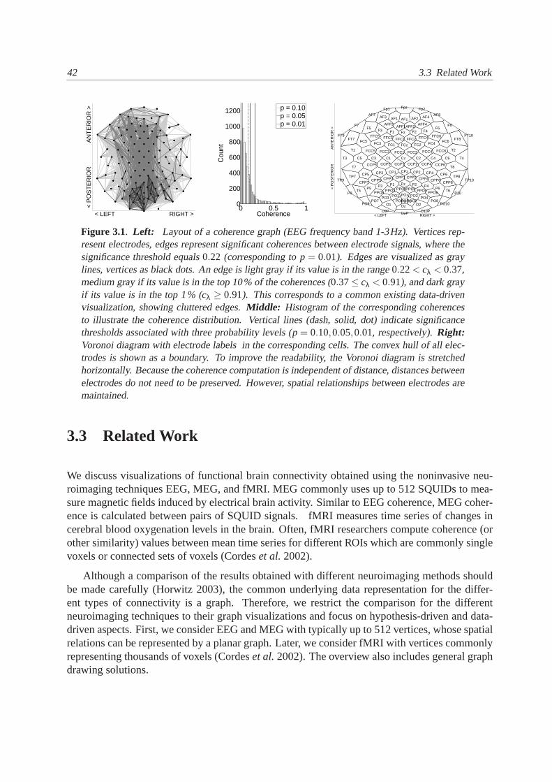
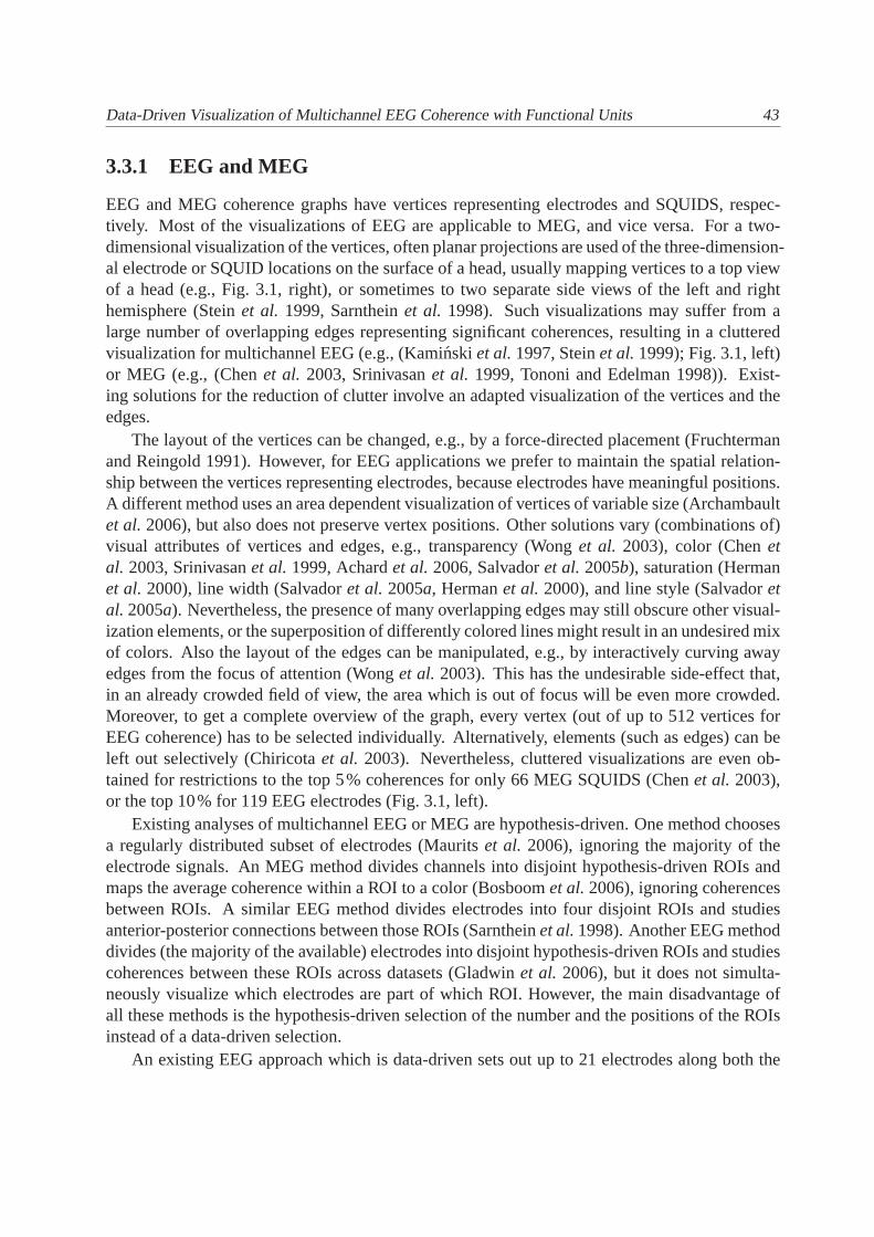
Figure 3.1. Left: Layout of a coherence graph (EEG frequency band 1-3Hz). Vertices rep-resent electrodes, edges represent significant coherences between electrode signals, where thesignificance threshold equals0.22 (corresponding top = 0.01). Edges are visualized as graylines, vertices as black dots. An edge is light gray if its value is in the range0.22< cλ < 0.37,medium gray if its value is in the top 10% of the coherences (0.37≤ cλ < 0.91), and dark grayif its value is in the top 1% (cλ ≥ 0.91). This corresponds to a common existing data-drivenvisualization, showing cluttered edges.Middle: Histogram of the corresponding coherencesto illustrate the coherence distribution. Vertical lines (dash, solid, dot) indicate significancethresholds associated with three probability levels (p = 0.10,0.05,0.01, respectively).Right:Voronoi diagram with electrode labels in the corresponding cells. The convex hull of all elec-trodes is shown as a boundary. To improve the readability, the Voronoi diagram is stretchedhorizontally. Because the coherence computation is independent of distance, distances betweenelectrodes do not need to be preserved. However, spatial relationships between electrodes aremaintained.
3.3 Related Work
We discuss visualizations of functional brain connectivity obtained using the noninvasive neu-roimaging techniques EEG, MEG, and fMRI. MEG commonly uses upto 512 SQUIDs to mea-sure magnetic fields induced by electrical brain activity. Similar to EEG coherence, MEG coher-ence is calculated between pairs of SQUID signals. fMRI measures time series of changes incerebral blood oxygenation levels in the brain. Often, fMRI researchers compute coherence (orother similarity) values between mean time series for different ROIs which are commonly singlevoxels or connected sets of voxels (Cordeset al.2002).
Although a comparison of the results obtained with different neuroimaging methods shouldbe made carefully (Horwitz 2003), the common underlying data representation for the differ-ent types of connectivity is a graph. Therefore, we restrictthe comparison for the differentneuroimaging techniques to their graph visualizations andfocus on hypothesis-driven and data-driven aspects. First, we consider EEG and MEG with typically up to 512 vertices, whose spatialrelations can be represented by a planar graph. Later, we consider fMRI with vertices commonlyrepresenting thousands of voxels (Cordeset al.2002). The overview also includes general graphdrawing solutions.
Data-Driven Visualization of Multichannel EEG Coherence with FunctionalUnits 43
3.3.1 EEG and MEG
EEG and MEG coherence graphs have vertices representing electrodes and SQUIDS, respec-tively. Most of the visualizations of EEG are applicable to MEG, and vice versa. For a two-dimensional visualization of the vertices, often planar projections are used of the three-dimension-al electrode or SQUID locations on the surface of a head, usually mapping vertices to a top viewof a head (e.g., Fig. 3.1, right), or sometimes to two separate side views of the left and righthemisphere (Steinet al. 1999, Sarntheinet al. 1998). Such visualizations may suffer from alarge number of overlapping edges representing significantcoherences, resulting in a clutteredvisualization for multichannel EEG (e.g., (Kaminskiet al.1997, Steinet al.1999); Fig. 3.1, left)or MEG (e.g., (Chenet al. 2003, Srinivasanet al. 1999, Tononi and Edelman 1998)). Exist-ing solutions for the reduction of clutter involve an adapted visualization of the vertices and theedges.
The layout of the vertices can be changed, e.g., by a force-directed placement (Fruchtermanand Reingold 1991). However, for EEG applications we prefer to maintain the spatial relation-ship between the vertices representing electrodes, because electrodes have meaningful positions.A different method uses an area dependent visualization of vertices of variable size (Archambaultet al.2006), but also does not preserve vertex positions. Other solutions vary (combinations of)visual attributes of vertices and edges, e.g., transparency (Wong et al. 2003), color (Chenetal. 2003, Srinivasanet al.1999, Achardet al.2006, Salvadoret al.2005b), saturation (Hermanet al. 2000), line width (Salvadoret al. 2005a, Hermanet al. 2000), and line style (Salvadoretal. 2005a). Nevertheless, the presence of many overlapping edges maystill obscure other visual-ization elements, or the superposition of differently colored lines might result in an undesired mixof colors. Also the layout of the edges can be manipulated, e.g., by interactively curving awayedges from the focus of attention (Wonget al. 2003). This has the undesirable side-effect that,in an already crowded field of view, the area which is out of focus will be even more crowded.Moreover, to get a complete overview of the graph, every vertex (out of up to 512 vertices forEEG coherence) has to be selected individually. Alternatively, elements (such as edges) can beleft out selectively (Chiricotaet al. 2003). Nevertheless, cluttered visualizations are even ob-tained for restrictions to the top 5% coherences for only 66 MEG SQUIDS (Chenet al. 2003),or the top 10% for 119 EEG electrodes (Fig. 3.1, left).
Existing analyses of multichannel EEG or MEG are hypothesis-driven. One method choosesa regularly distributed subset of electrodes (Mauritset al. 2006), ignoring the majority of theelectrode signals. An MEG method divides channels into disjoint hypothesis-driven ROIs andmaps the average coherence within a ROI to a color (Bosboomet al.2006), ignoring coherencesbetween ROIs. A similar EEG method divides electrodes into four disjoint ROIs and studiesanterior-posterior connections between those ROIs (Sarntheinet al.1998). Another EEG methoddivides (the majority of the available) electrodes into disjoint hypothesis-driven ROIs and studiescoherences between these ROIs across datasets (Gladwinet al. 2006), but it does not simulta-neously visualize which electrodes are part of which ROI. However, the main disadvantage ofall these methods is the hypothesis-driven selection of thenumber and the positions of the ROIsinstead of a data-driven selection.
An existing EEG approach which is data-driven sets out up to 21 electrodes along both the
44 3.3 Related Work
rows and columns of a matrix as a tiled display (Kaminski et al.1997, Franaszczuket al.1994).The result is a square contingency table showing coherence values for all possible electrode pairs.Each table entry is a square in which coherence is displayed between the two correspondingelectrode signals as a function of frequency. By arranging the electrodes along the rows andthe columns of the matrix, the spatial relations are lost. Asa result, consecutive entries in thetable do not need to imply coherence between pairs of signalsrecorded at adjacent electrodes onthe scalp. Similarly, a square contingency table is createdfor 78 MEG SQUIDS sorted into fourhypothesis-driven ROIs (Srinivasanet al.1999) (left/right, anterior/posterior). Each table entryissquare with the coherence of the corresponding signals mapped to a color. A different data-drivenEEG approach first localizes dipoles corresponding to maximally independent components inthe data, and then calculates and visualizes coherence between dipole activities (Delormeetal. 2002, Makeiget al.2004, De Vico Fallaniet al.2007). However, dipole source solutions arenot unique (Srinivasan 1999).
Another approach is restricted to local EEG coherence, which is defined as the coherencebetween two spatially neighboring electrodes (Rappelsberger and Petsche 1988, Schacket al.1999). It requires additional methods to study coherences between electrodes which are notdirect spatial neighbors. Another visualization creates amap of topographic submaps (Nolteetal. 2004), with one submap for each electrode visualizing the coherence between itself and everyother electrode. It does not explicitly visualize coherence between electrodes by connecting lines.As a consequence, every topographic submap (out of up to 512 submaps) needs to be studiedseparately to obtain a complete overview. Another drawbackis that local coherences dominatethe visualization (Nolteet al. 2004). A subselection of two topographic submaps out of 128 ismade by Knyazevaet al. (2006), without providing a complete overview of all coherences.
3.3.2 fMRI
For fMRI coherence, usually a limited number of so-called seed (or reference) voxels is selectedon the basis of prior anatomical or functional information.However, the anatomy may be ab-normal, and the choice of seed points may affect the results (Cordeset al. 2002). Nonetheless,an individual seed point or a spatially connected set of voxels including a seed point is con-sidered as a ROI having a (mean) time series. Vertices represent ROIs and can be visualizedthree-dimensionally (Worsleyet al. 2005) or two-dimensionally. A two-dimensional visualiza-tion uses, e.g., a planar projection of three-dimensional ROI positions or an approximation offunctional distances by graphical distances using metric multidimensional scaling (Salvadoretal. 2005a). An edge represents a significant similarity between two ROI time series. The visual-ization of edges as lines may lead to clutter (Achardet al.2006, Salvadoret al.2005b, Salvadoret al.2005a, Worsleyet al.2005).
Filtering edges may still lead to cluttered visualizations(Achardet al.2006). Other visualiza-tions set out ROIs along the rows and columns, thus obtaininga square contingency table. Eachtable entry is a square with a similarity value between the two corresponding signals mappedto a color (Srinivasanet al. 1999, Achardet al. 2006). Existing data-driven graph clusteringalgorithms include hierarchical cluster analysis (Cordeset al.2002) and independent componentanalysis (ICA) (Delormeet al.2002, Makeiget al.2004, van de Venet al.2004). The result of
Data-Driven Visualization of Multichannel EEG Coherence with FunctionalUnits 45
hierarchical cluster analysis can be visualized as a dendrogram (Salvadoret al.2005a), showingthe ROIs as leaves of a binary tree, thus losing the spatial relations between the ROIs. Also, ROIscan be visualized as colored volumes of interest (van de Venet al.2004) which may occlude eachother. For the same reason, we do not favor three-dimensional EEG visualizations. Alternatively,ROIs can be visualized on anatomical slices (Cordeset al. 2002, Salvadoret al. 2005a, Sunetal. 2004). However, a large number of two-dimensional slices isrequired to obtain a completeoverview of a three-dimensional volume. Sometimes, instead of an explicit visualization of theconnection between ROIs (e.g., with a line), all ROIs in one cluster are colored identically, withdifferent colors and/or separate slices for different clusters (Salvadoret al.2005a).
3.3.3 Conclusion
The overview of related work has concentrated on the requirements we posed on an EEG coher-ence visualization: it should be (1) data-driven, (2) preserve electrode locations, (3) minimizevisual clutter, and (4) present an overview. Many of the discussed methods still suffer from vi-sual clutter or relocate vertices and edges and therefore donot meet requirement (2) or (3). Onthe other hand, existing methods which do meet requirements(2,3) are hypothesis-driven, thusfailing to meet our requirement (1). In summary, the method proposed in this chapter combinesa number of features which no single technique currently provides.
3.4 Data Representation
3.4.1 Experimental Setup
Here, brain responses from two groups of five younger (34±10 years, mean± standard devi-ation) and five older (62±8 years) adults are studied, which were recorded using an EEGcapwith 119 scalp electrodes. During a so-called P300 experiment, each participant was instructedto count target tones of 2000Hz (probability 0.15), alternated with standard tones of 1000Hz(probability 0.85) which were to be ignored. After the experiment, the participant had to reportthe number of perceived target tones. For each dataset, brain responses to 20 target tones wererecorded inL = 20 segments of 1s. EEG coherence is influenced by the choice ofreference. Wechose to use an average reference, which is a close-to-optimal approximation to a reference-freerecording in the case of 128 electrodes (Mauritset al.2006, Nunezet al.1997).s
A procedure from Neurospec was adopted to compute the coherence (www.neurospec.org ). We first averaged over segments and then over adjacent spectral lines in predefined fre-quency bands. Frequencies between 1 and 30Hz are typically studied clinically. We calculatedthe average coherence within five EEG frequency bands (1-3, 4-7, 8-12, 13-20, and 21-30Hz),because EEG synchrony varies with frequency (Mauritset al.2006, Nunezet al.1997). For 119electrodes, in total 7021 coherence values were computed per frequency band. If the conduc-tive gel accidentally connected two adjacent electrodes, very high coherences were measured.Coherences higher than 0.99 were therefore ignored. Typically, this threshold value eliminatesapproximately 0.01% of the coherences. Note also that usingEqn. 3.1 for determining signif-
46 3.5 FU Detection
icance levels is a coarse approximation, since it does not take the number of spectral lines perband into account. However, this approximation only overestimates the significance level, anddoes not influence the visualization method itself.
3.4.2 EEG Coherence Graph
The data are represented by acoherence graphwith vertices representing electrodes. Coher-ences above the significance threshold (Eqn. 3.1) are represented by edges, coherences belowthe threshold are ignored. To determine spatial relationships between electrodes, a Voronoi dia-gram is employed which partitions the plane into regions of points with the same nearest vertex(Voronoi 1908). For EEG data, the vertex set equals the set ofelectrode positions (Fig. 3.1, right).The vertices are referred to as (Voronoi) centers, the region boundaries as (Voronoi) polygons.The area enclosed by a polygon is called a (Voronoi) cell. We call two cellsVoronoi neighborsif they have a boundary in common. A collection of cellsC is calledVoronoi-connectedif for apair φ0,φn ∈C there is a sequenceφ0,φ1, ...,φn of cells inC with each pairφi−1,φi consisting ofVoronoi neighbors. Cells, vertices, and electrodes are interchangeable for the use with the terms“Voronoi neighbor” and “Voronoi-connected”.
3.5 FU Detection
Whereas there are many unsupervised graph clustering methods, e.g., hierarchical clustering andICA (see Section 3.3), our choice is motivated by the type of cluster we desire. As a resultof volume conduction (Lachauxet al. 1999), multiple electrodes can record a signal from asingle source. Consequently, a spatially connected set of electrodes recording similar signals isconsidered as a data-driven ROI (a cluster). Such a ROI is referred to as functional unit (FU) andis represented in the EEG coherence graph by a clique consisting of a set of spatially connectedvertices.
Recall that larger ROIs are assumed to correspond to strongersource signals and are consid-ered to be more interesting. Therefore, our first method for FU detection is primarily based onthe detection of maximal cliques (Bron and Kerbosch 1973, Tomita et al. 2006). We adapt thismethod to detect spatially connected sets of vertices (ten Caatet al.2007d). Our second methodfor FU detection is based on watersheds, an efficient method for detecting spatially connectedsegments (Roerdink and Meijster 2000). We adapt this method to detected cliques in a greedyway (ten Caatet al. 2007e). However, it does not avoid the oversegmentation problem well-known for watersheds. A third method, also based on watersheds, reduces over-segmentation.
3.5.1 Maximal Clique Based (MCB) Method
Maximal Cliques
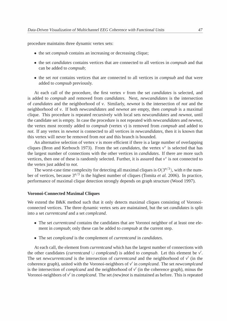
Bron and Kerbosch (B&K) (Bron and Kerbosch 1973) developed a method to detect all maximalcliques in a graph. It first branches the problem, and bounds unsuccessful branches. Its recursive
Data-Driven Visualization of Multichannel EEG Coherence with FunctionalUnits 47
procedure maintains three dynamic vertex sets:
• the setcompsubcontains an increasing or decreasing clique;
• the setcandidatescontains vertices that are connected to all vertices incompsuband thatcan be added tocompsub;
• the setnot contains vertices that are connected to all vertices incompsuband that wereadded tocompsubpreviously.
At each call of the procedure, the first vertexv from the setcandidatesis selected, andis added tocompsuband removed fromcandidates. Next, newcandidatesis the intersectionof candidatesand the neighborhood ofv. Similarly, newnotis the intersection ofnot and theneighborhood ofv. If both newcandidatesandnewnotare empty, thencompsubis a maximalclique. This procedure is repeated recursively with local setsnewcandidatesandnewnot, untilthe candidate set is empty. In case the procedure is not repeated withnewcandidatesandnewnot,the vertex most recently added tocompsub(vertexv) is removed fromcompsuband added tonot. If any vertex innewnotis connected to all vertices innewcandidates, then it is known thatthis vertex will never be removed fromnot and this branch is bounded.
An alternative selection of vertexv is more efficient if there is a large number of overlappingcliques (Bron and Kerbosch 1973). From the setcandidates, the vertexv∗ is selected that hasthe largest number of connections with the other vertices incandidates. If there are more suchvertices, then one of these is randomly selected. Further, it is assured thatv∗ is not connected tothe vertex just added tonot.
The worst-case time complexity for detecting all maximal cliques isO(3n/3), with n the num-ber of vertices, because 3n/3 is the highest number of cliques (Tomitaet al. 2006). In practice,performance of maximal clique detection strongly depends on graph structure (Wood 1997).
Voronoi-Connected Maximal Cliques
We extend the B&K method such that it only detects maximal cliques consisting of Voronoi-connected vertices. The three dynamic vertex sets are maintained, but the setcandidatesis splitinto a setcurrentcandand a setcomplcand.
• The setcurrentcandcontains the candidates that are Voronoi neighbor of at least one ele-ment incompsub; only these can be added tocompsubat the current step.
• The setcomplcandis the complement ofcurrentcandin candidates.
At each call, the element fromcurrentcandwhich has the largest number of connections withthe other candidates (currentcand∪ complcand) is added tocompsub. Let this element bev′.The setnewcurrentcandis the intersection ofcurrentcandand the neighborhood ofv′ (in thecoherence graph), united with the Voronoi-neighbors ofv′ in complcand. The setnewcomplcandis the intersection ofcomplcandand the neighborhood ofv′ (in the coherence graph), minus theVoronoi-neighbors ofv′ in complcand. The set(new)notis maintained as before. This is repeated
48 3.5 FU Detection
until newcurrentcandis empty. Ifnewnotis also empty, thencompsubis a Voronoi-connectedmaximal clique.
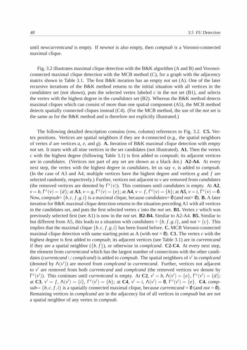
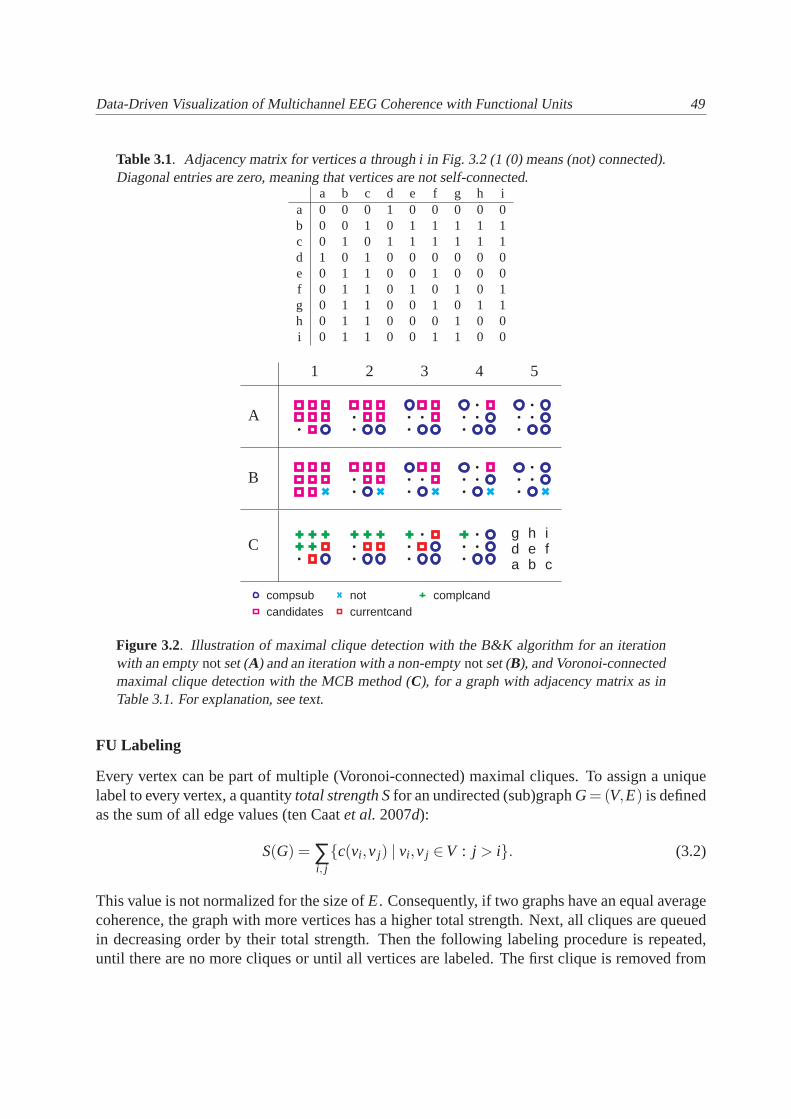
Fig. 3.2 illustrates maximal clique detection with the B&K algorithm (A and B) and Voronoi-connected maximal clique detection with the MCB method (C), for a graph with the adjacencymatrix shown in Table 3.1. The first B&K iteration has an emptynot set (A). One of the laterrecursive iterations of the B&K method returns to the initialsituation with all vertices in thecandidatesset (not shown), puts the selected vertex labeledc in the not set (B1), and selectsthe vertex with the highest degree in thecandidatesset (B2). Whereas the B&K method detectsmaximal cliques which can consist of more than one spatial component (A5), the MCB methoddetects spatially connected cliques instead (C4). (For the MCB method, the use of thenot set isthe same as for the B&K method and is therefore not explicitly illustrated.)
The following detailed description contains (row, column)references to Fig. 3.2.C5. Ver-tex positions. Vertices are spatial neighbors if they are 4-connected (e.g., the spatial neighborsof vertexd are verticesa, e, andg). A. Iteration of B&K maximal clique detection with emptynot set. It starts with all nine vertices in the set candidates (not illustrated).A1. Then the vertexc with the highest degree (following Table 3.1) is first added to compsub; its adjacent verticesare incandidates. (Vertices not part of any set are shown as a black dot.)A2-A4. At everynext step, the vertex with the highest degree incandidates, let us sayv, is added tocompsub.(In the case of A3 and A4, multiple vertices have the highest degree and verticesg and f areselected randomly, respectively.) Further, vertices not adjacent tov are removed fromcandidates(the removed vertices are denoted byΓc(v)). This continues untilcandidatesis empty. AtA2,v= b, Γc(v) = {d}; atA3, v= g, Γc(v) = {e}; atA4, v= f , Γc(v) = {h}; atA5, v= i, Γc(v) = /0.Now,compsub= {b,c, f ,g, i} is a maximal clique, becausecandidates= /0 (andnot= /0). B. A lateriteration for B&K maximal clique detection returns to the situation preceding A1 with all verticesin the candidates set, and puts the first selected vertexc into thenot set.B1. Vertexc which waspreviously selected first (see A1) is now in thenot set.B2-B4.Similar to A2-A4.B5. Similar tobut different from A5, this leads to a situation withcandidates= {b, f ,g, i}, andnot = {c}. Thisimplies that the maximal clique{b,c, f ,g, i} has been found before.C. MCB Voronoi-connectedmaximal clique detection with same starting point as A (withnot = /0). C1. The vertexc with thehighest degree is first added tocompsub; its adjacent vertices (see Table 3.1) are incurrentcandif they are a spatial neighbor ({b, f}), or otherwise incomplcand. C2-C4. At every next step,the element fromcurrentcandwhich has the largest number of connections with the other candi-dates (currentcand∪ complcand) is added tocompsub. The spatial neighbors ofv′ in complcand(denoted byΛ(v′)) are moved fromcomplcandto currentcand. Further, vertices not adjacentto v′ are removed from bothcurrentcandandcomplcand(the removed vertices we denote byΓc(v′)). This continues untilcurrentcandis empty. AtC2, v′ = b, Λ(v′) = {e}, Γc(v′) = {d};at C3, v′ = f , Λ(v′) = {i}, Γc(v′) = {h}; at C4, v′ = i, Λ(v′) = /0, Γc(v′) = {e}. C4. comp-sub= {b,c, f , i} is a spatially connected maximal clique, becausecurrentcand= /0 (andnot = /0).Remaining vertices incomplcandare in the adjacency list of all vertices incompsubbut are nota spatial neighbor of any vertex incompsub.
Data-Driven Visualization of Multichannel EEG Coherence with FunctionalUnits 49
Table 3.1. Adjacency matrix for verticesa throughi in Fig. 3.2 (1 (0) means (not) connected).Diagonal entries are zero, meaning that vertices are not self-connected.
a b c d e f g h ia 0 0 0 1 0 0 0 0 0b 0 0 1 0 1 1 1 1 1c 0 1 0 1 1 1 1 1 1d 1 0 1 0 0 0 0 0 0e 0 1 1 0 0 1 0 0 0f 0 1 1 0 1 0 1 0 1g 0 1 1 0 0 1 0 1 1h 0 1 1 0 0 0 1 0 0i 0 1 1 0 0 1 1 0 0
1 2 3 4 5
A
B
Ca b cd e fg h i
compsubcandidates
notcurrentcand
complcand
Figure 3.2. Illustration of maximal clique detection with the B&K algorithm for an iterationwith an emptynotset (A) and an iteration with a non-emptynotset (B), and Voronoi-connectedmaximal clique detection with the MCB method (C), for a graph with adjacency matrix as inTable 3.1. For explanation, see text.
FU Labeling
Every vertex can be part of multiple (Voronoi-connected) maximal cliques. To assign a uniquelabel to every vertex, a quantitytotal strength Sfor an undirected (sub)graphG= (V,E) is definedas the sum of all edge values (ten Caatet al.2007d):
S(G) = ∑i, j{c(vi ,v j) | vi ,v j ∈V : j > i}. (3.2)
This value is not normalized for the size ofE. Consequently, if two graphs have an equal averagecoherence, the graph with more vertices has a higher total strength. Next, all cliques are queuedin decreasing order by their total strength. Then the following labeling procedure is repeated,until there are no more cliques or until all vertices are labeled. The first clique is removed from
50 3.5 FU Detection
the queue, and all its vertices are assigned a unique label and are removed from the other cliques.If necessary, the changed cliques are separated into Voronoi-connected components. For allchanged cliques, the total strength is recomputed before they are put in the appropriate positionin the sorted queue. After completion of the labeling procedure, every set of identically labeledvertices is an FU.
3.5.2 Watershed Based (WB) Method
As an alternative to the MCB method, we present a greedy methodapproximating maximalcliques on the basis of the watershed transform (Roerdink andMeijster 2000). In the usualwatershed algorithm, a subset of all local minima is selected as markers. Markers are labeledand are associated with basins. Basins contain vertices withthe same label as the correspond-ing marker and are extended as follows, using the watershed implementation based on orderedqueues (Beucher and Meyer 1993). The first vertexv is removed from a queue of vertices sortedin decreasing order of priority. Every unlabeled neighborv′ of v receives the same label asv andis put into the queue with a priority depending on the value ofv′, but not higher than the priorityof v. This continues until the queue is empty.
Now we modify the usual watershed transform in order to obtain spatially connected setsof electrodes, where all electrodes in a given set have recorded mutually significantly coherentsignals. This modification concerns two steps in the watershed transform: (i) choice of mark-ers; (ii) use of an edge queue instead of a vertex queue. We explain these two points in moredetail.
First, we define a marker as an electrode recording a signal that is locally maximally coherentwith signals of its spatially neighboring electrodes. Because the EEG coherence graph has edgevalues instead of vertex values, we first assign a coherence value to each vertex by computing theaverage of the edge values between this vertex and all its Voronoi neighbors. Then, we select allvertices which are local maxima as markers to be associated with basins, because those verticesare locally maximally similar to their spatially neighboring vertices. Note that we chooseall localmaxima as markers, instead of a small subset as is usually done when the watershed algorithmis applied to digital images. In our case the over-segmentation problem is less severe, becausethe number of electrodes is an order of magnitude smaller than the number of pixels in an image.If the number of basins (i.e., clusters) found is still too large, we can suppress basins below acertain size in a post-processing step.
The second point concerns the type of queue we use. Whereas theusual queue-based im-plementation of the watershed transform applied to digitalimages uses a vertex queue sorted inincreasing order of value (Beucher and Meyer 1993), we use an edge queue sorted in decreasingorder of coherence value. (The vertex values are only used for defining the markers.) In casethe coherence graph has multiple identical edge values (which did not occur for our datasets), anordered queue consisting of queues with identically valuedelements can be used, as for digitalimages which usually contain multiple identically valued vertices (Beucher and Meyer 1993).
The WB method for greedy Voronoi-connected clique detectionmaintains the following dy-namic vertex sets.
Data-Driven Visualization of Multichannel EEG Coherence with FunctionalUnits 51
• bsni contains a sorted list of the vertices in basini.
• L(v) contains the basin label of vertexv.
• adjCohBsni contains a list of vertices (sorted by vertex number) which are adjacent toeachof the vertices inbsni in the coherence graph.
• queuecontains edges in decreasing order. When vertexv receives a label, an edgee =(v,v′) is added toqueuefor each unlabeled Voronoi neighborv′ of v, provided that thecorresponding edge value exceeds the significance threshold (Eqn. 3.1).
(Step 1) The edge queue is initialized with edges (corresponding with a significant coherence)between markers and their Voronoi neighbors. The first edge(v,v′) in this queue correspondsto the highest similarity (coherence) between any vertexv′ outside and a Voronoi neighboringvertexv inside a basin. Therefore, vertexv′ is the first candidate to be added to a basin.
(Step 2) The main procedure consists of the following steps.Remove the first edge, saye=(v,v′) from queue. In case vertexv′ was also labeled between the insertion and removal ofe=(v,v′), nothing is done and the procedure continues with a new edge.Otherwise (v′ is unla-beled), there are two cases. (i) In casev′ ∈ adjCohBsnL(v) (ln. 19), v′ receives labelL(v) and(ii) adjCohBsnL(v) is replaced by its intersection with the neighborhood ofv′ in the coherencegraph (ln. 21); (iii)v′ is added tobsnL(v) (ln. 22); (iv) queueis extended with the edges be-tweenv′ and its Voronoi-neighbors (ln. 23-27), provided that corresponding edge values exceedthe significance threshold. In the other case, ifv′ /∈ adjCohBsnL(v), v′ is not labeled (yet). Thisprocedure is repeated untilqueueis empty. Each basin then corresponds to an FU.
The time complexity of the WB method isO(n2 logn), with n the number of vertices (tenCaatet al.2007e), which can be seen as follows. Step 1 consists of creating a sorted edge queue,so has complexitynlogn, because the order of the number of edges between Voronoi neighbors isthe same as the order of the total number of edges in a planar graph (which isO(n)). In step 2, thefollowing steps are executedO(n) times with sorted vertex sets of at mostn vertices: (i) binarysearch for the presence of a vertex in a vertex set (O(logn)); (ii) binary search for the insertion ofa vertex into a vertex set (O(logn)); (iii) intersecting two vertex sets (O(n)); (iv) insertion of atmostn edges into the sorted queue(O(nlogn)). Step (iv) has a higher time complexity than (i)-(iii). Therefore, the time complexity for step 2 (O(n2 logn)) is higher than for step 1 (O(nlogn)),which makes the total time complexity of the WB method equal toO(n2 logn).
3.5.3 Improved Watershed Based (IWB) Method
Over-segmentation is a potential problem of the WB method. Toreduce over-segmentation, twospatially neighboring FUs are merged if their union is a clique in the coherence graph. To obtainthe improved watershed based (IWB) algorithm (Alg. 1) we insert lines 11-15 and lines 29-42 in the pseudocode of the WB algorithm (see also (ten Caatet al. 2007e)). In words, thedifference between the WB and IWB method is the following. In case vertexv′ was labeledbetween the insertion and removal ofe= (v,v′), nothing is done if the label ofv′ is equal to thelabel ofv. Otherwise (L(v′) 6= L(v)), see line 29), the following steps are executed consecutively
52 3.5 FU Detection
< LEFT RIGHT >
< P
OS
TE
RIO
R
AN
TE
RIO
R >
< LEFT RIGHT >
< P
OS
TE
RIO
R
AN
TE
RIO
R >
< LEFT RIGHT >
< P
OS
TE
RIO
R
AN
TE
RIO
R >
0.3
0.4
0.5
0.6
0.7
0.8
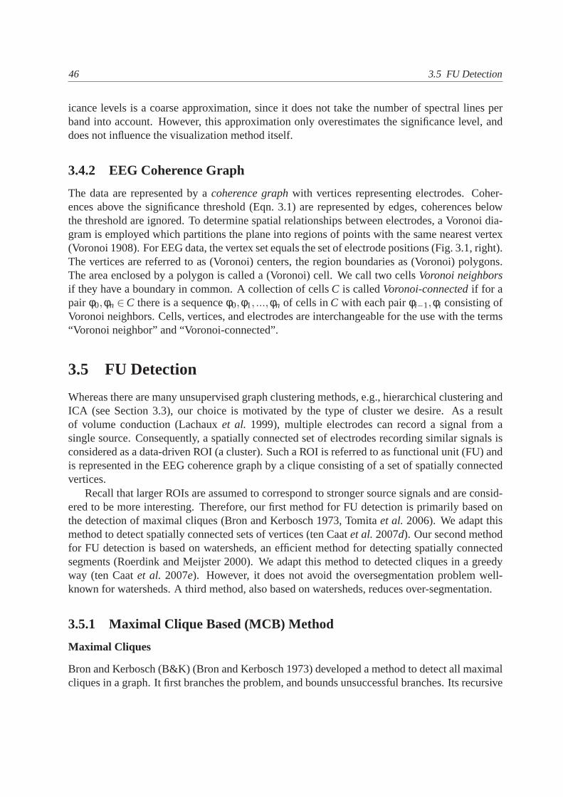
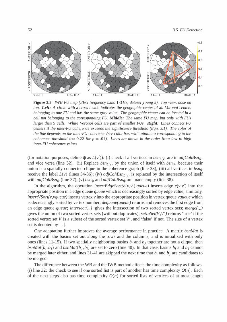
Figure 3.3. IWB FU map (EEG frequency band1-3Hz, dataset young 5). Top view, nose ontop. Left: A circle with a cross inside indicates the geographic center of all Voronoi centersbelonging to one FU and has the same gray value. The geographic center can be located in acell not belonging to the corresponding FU.Middle: The same FU map, but only with FUslarger than5 cells. White Voronoi cells are part of smaller FUs.Right: Lines connect FUcenters if the inter-FU coherence exceeds the significance threshold (Eqn. 3.1). The color ofthe line depends on the inter-FU coherence (see color bar, with minimum corresponding to thecoherence thresholdφ ≈ 0.22 for p = .01). Lines are drawn in the order from low to highinter-FU coherence values.
(for notation purposes, defineψ asL(v′)): (i) check if all vertices inbsnL(v) are inadjCohBsnψ,and vice versa (line 32). (ii) ReplacebsnL(v) by the union of itself withbsnψ, because theirunion is a spatially connected clique in the coherence graph(line 33); (iii) all vertices inbsnψreceive the labelL(v) (lines 34-36); (iv)adjCohBsnL(v) is replaced by the intersection of itselfwith adjCohBsnψ (line 37); (v)bsnψ andadjCohBsnψ are made empty (line 38).
In the algorithm, the operationinsertEdgeSort(e(v,v′),queue)inserts edgee(v,v′) into theappropriate position in a edge queuequeuewhich is decreasingly sorted by edge value; similarly,insertVSort(v,vqueue)inserts vertexv into the appropriate position in vertex queuevqueuewhichis decreasingly sorted by vertex number;dequeue(queue)returns and removes the first edge froman edge queuequeue; intersect(.,.) gives the intersection of two sorted vertex sets;merge(.,.)gives the union of two sorted vertex sets (without duplicates);setInSet(V ,V′) returns ‘true’ if thesorted vertex setV is a subset of the sorted vertex setV ′, and ‘false’ if not. The size of a vertexset is denoted by| . |.
One adaptation further improves the average performance inpractice. A matrixbsnMatiscreated with the basins set out along the rows and the columns, and is initialized with onlyones (lines 11-15). If two spatially neighboring basinsbi andb j together are not a clique, thenbsnMat(bi ,b j) andbsnMat(b j ,bi) are set to zero (line 40). In that case, basinsbi andb j cannotbe merged later either, and lines 31-41 are skipped the next time thatbi andb j are candidates tobe merged.
The difference between the WB and the IWB method affects the time complexity as follows.(i) line 32: the check to see if one sorted list is part of another has time complexityO(n). Eachof the next steps also has time complexityO(n) for sorted lists of vertices of at most length
Data-Driven Visualization of Multichannel EEG Coherence with FunctionalUnits 53
n: (ii) line 33: taking the union of two sorted lists, (iii) lines 34-36: labeling a list, (iv) line 37:intersecting two sorted lists, (v) line 38: making lists empty. Steps (i)-(v) are executedO(n) times(recall that the order of the number of edges between Voronoineighbors inqueueis O(n)). Thus,the time complexity of the IWB adaptation isO(n2) and the time complexity for the completeIWB algorithm is the same as for the WB method, i.e.,O(n2 logn).
3.6 FU Visualization
3.6.1 FU Map for Individual Dataset Analysis
FU Map Coloring
An FU map visualizes each FU as a set of Voronoi cells with identical gray value, with differentgray values for adjacent FUs. The problem of coloring the FUscorresponds to the coloring of aplane graph, assigning different colors to adjacent vertices. Humans can detect one color amonga total of about five to seven different colors rapidly and accurately (Healey 1996), whereas therecan be more than five FUs. However, for any plane graph, four colors are sufficient (Robertsonet al.1996).
To find a four-coloring of the FUs, the FUs are sorted by their number of neighboring FUs,from high to low. From a set of four available colors, each FU is assigned (one by one) acolor different from its neighbors. If there are already four different colors among its neighbors,there is an impasse. To solve the impasse, we make use of ac-d Kempe chain, which is aconnected component of a colored graph with vertices colored c or d. Interchanging the twocolors in a Kempe chain is referred to as Kempe chaining (Morgenstern and Shapiro 1991). Thisis executed randomly with neighbors of the impasse FU, untilthe impasse is solved. If thisdoes not terminate within a certain number of attempts, thenthe FUs are sorted randomly beforerestarting the coloring procedure.
Instead of four different colors, we use four different graylevels (Fig. 3.3, left, middle).Because larger FUs are considered to be more interesting, only FUs larger than 5 cells are con-sidered. White Voronoi cells are part of smaller FUs.
FU Map Connections
Given the FUs, we define theinter-FU coherence c′ at frequencyλ between two functional unitsW1 andW2 as the sum of the coherence values between one vertex inW1 and the other vertex inW2, scaled by the total number of edges betweenW1 andW2 (ten Caatet al.2007d):
c′λ(W1,W2) =∑i, j{cλ(vi ,v j) | vi ∈W1,v j ∈W2}
|W1| · |W2|. (3.3)
Here, |Wi| indicates the number of vertices inWi. Note that coherences between any pair ofvertices are taken into account, to normalize for the size ofthe FUs.

54 3.6 FU Visualization
Algorithm 1 WB pseudocode with adaptations (ln. 11-15, 29-42) to obtain the IWB method.INPUT: V is the vertex set;marker(i)= markeri; c(v,v′) = coherence(v,v′) = c(v′,v);
adjCohv = {v′ ∈V | c(v,v′) ≥ φ}; φ = sign. threshold; adjVorv = {v′ ∈V | v′ ∈ Vor.-neighborsv & v′ ∈ adjCohv};{adjCohv, adjVorv are both sorted by vertex number}
OUTPUT: bsni is basini (i.e., an FU) sorted by vertex numberINITIALIZATION :1: queue← /0 {queue of edges}2: for all v∈V do3: L(v)← 0 {L(v) = label of vertexv}4: end for5: for i = 1 to |marker| do6: bsni ← marker(i); v← marker(i); L(v)← i; adjCohBsnL(v) ← adjCohv7: for all v′ ∈ adjVorv do8: insertEdgeSort(e(v,v′),queue)9: end for
10: end for11: for i = 1 to |marker| do12: for j = 1 to |marker| do13: bsnMat(i, j)← 1 {IWB modification}14: end for15: end forMAIN :16: while queue6= /0 do17: e(v,v′)← dequeue(queue)18: if L(v′) = 0 then19: if v′ ∈ adjCohBsnL(v) then20: L(v′)← L(v)21: adjCohBsnL(v)←intersect(adjCohBsnL(v),adjCohv′ )22: bsnL(v)← insertVSort(v′,bsnL(v))23: for all v∗ ∈ adjVorv′ do24: if L(v∗) = 0 then25: insertEdgeSort(e(v′,v∗),queue)26: end if27: end for28: end ifBEGIN IWB29: else30: if (L(v′) 6= L(v)) and (bsnMat(L(v′),L(v)) 6= 0) then31: ψ← L(v′)32: if setInSet(bsnL(v),adjCohBsnψ) andsetInSet(bsnψ,adjCohBsnL(v)) then33: bsnL(v)←merge(bsnL(v),bsnψ)34: for all w′ ∈ bsnψ do35: L(w′)← L(v)36: end for37: adjCohBsnL(v) ← intersect(adjCohBsnL(v),adjCohBsnψ)38: bsnψ = /0; adjCohBsnψ = /039: else40: bsnMat(L(v),ψ)← 0; bsnMat(ψ,L(v))← 041: end if42: end ifEND IWB43: end if44: end while

Data-Driven Visualization of Multichannel EEG Coherence with FunctionalUnits 55
A line is drawn between FU centers if the corresponding inter-FU coherence exceeds a thresh-old (Fig 3.3, right). We consistently choose this thresholdto be equal to the significance thresh-old (Eqn. 3.1), as we already used this threshold to determine the initial graph.
3.6.2 Data-Driven Group Analysis
FU maps differ from individual to individual, making group analysis difficult. Therefore, wedevelop a data-driven method for group coherence analysis which detects common features ina collection of individual FU maps. Group coherence analyses are commonly based on groupmeans of coherences of interest. We show how our data-drivenROIs, i.e., the FUs, lead to adata-driven selection of coherences of interest.
Group Mean Coherence Map
We define agroup mean coherence graphas the graph containing the mean coherence for everyelectrode pair computed across a group, with vertices representing electrodes and edges contain-ing coherence values. To obtain a data-driven coherence visualization for a group, the groupmean coherence graph is thresholded, maintaining only the edges with a value exceeding thecoherence threshold (Eqn. 3.1). Next, an FU map is created for the group mean coherence graph,referred to asgroup mean coherence map.
Group FU Size Map
A group FU size map visualizes the average FU size for every electrode across a group, based onthe FU maps for every individual dataset. The average FU sizesof an electrodev is computed as
s(v) = ∑all datasets
{|W| | v∈W}#datasets
. (3.4)
with W the FU containingv in every FU map. The values for an electrode is mapped to thegray value of its corresponding Voronoi cell, similar to a (gray scale) topographic map (ten Caatet al. 2007c). Lighter gray is used for higher average FU sizes, as highervalues commonlycorrespond to lighter gray in gray scale images.
Consequently, a light Voronoi cell indicates that the corresponding electrode is on averagepart of large FUs.
3.7 Results
Throughout this section, we usep = 0.01. The corresponding coherence threshold isφ ≈0.22 (Eqn. 3.1).
56 3.7 Results
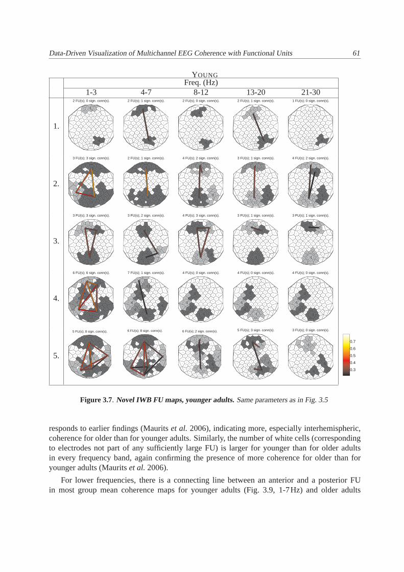
3.7.1 FU Map
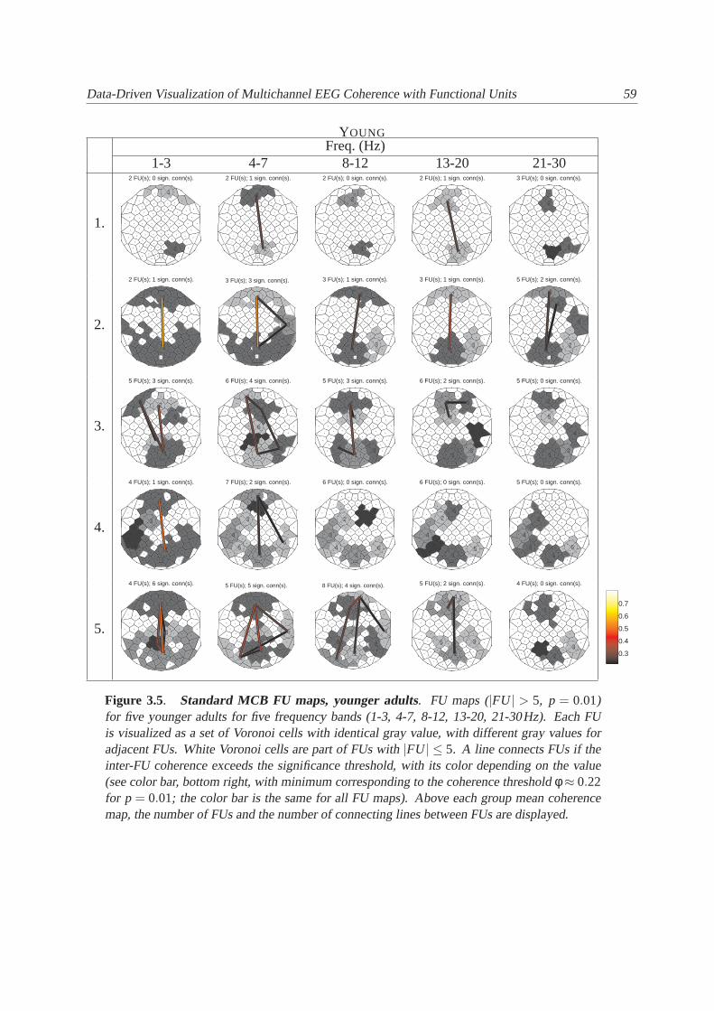
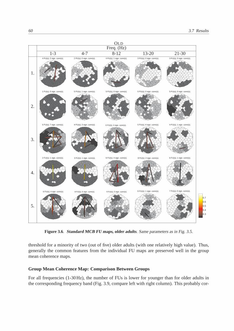
For a comparison of FU maps obtained with the three differentFU detection methods, seeFig. 3.4. FU maps for the five datasets in each group and each ofthe five frequency bandsare shown in Fig. 3.5 to 3.8 for the MCB and IWB method.
FU detection with the (non-optimized) MCB method was faster for smaller FU sizes, takingapproximately 1s for datasets with small FUs, and up to 2h forthe dataset with the largest FU.FU detection with the (non-optimized) WB method took around 0.04±0.02s (max. 0.14s) andwith the (non-optimized) IWB method around 0.05±0.04s (max. 0.25s). Consequently, the WBand IWB methods are up to a factor of 100,000 times faster than the MCB method for this typicalmultichannel EEG setting with 128 channels.
Because the MCB method is assumed to obtain the most interesting FUs corresponding to thestrongest source signals (Section 3.5), it is here considered as the gold standard. We comparedthe WB and the IWB method with the MCB method, and made an illustrative selection of seven(out of fifty) cases for a detailed discussion (Fig. 3.4). Theselection includes those settings (acombination of participant and frequency band) which result in the largest difference between theMCB, WB, and IWB method. The order of the seven illustrations is chosen such that it facilitatesthe discussion.
i. The one anterior FU detected by the MCB method is represented by two (smaller) spatiallyconnected anterior FUs by the WB method, whereas the IWB methodmerges two anteriorFUs. Because the WB and IWB methods both follow a greedy approach, the anterior FUsdo not correspond exactly to the anterior FU of the MCB FU map. Because the IWBmethod merges FUs during segmentation (and not afterwards,such as with hierarchicalwatersheds (Schultzet al.2007)), the vertices in the large anterior FU of the IWB FU mapdo not correspond exactly to the vertices that are part of thesmaller anterior FUs obtainedby the WB method.
ii. Although multiple anterior FUs are obtained with the WB method, they are smaller thanthe minimum size and are therefore not shown, whereas the IWB method merges smallerFUs into an anterior FU identical to the anterior FU found with the MCB method.
iii. This is one of the occurrences of the maximal absolute difference in the number of FUs be-tween the MCB (6 FUs) and IWB method (3 FUs). Nevertheless, the connection betweenan anterior and a posterior region which is visible in the MCB FU map is preserved in theIWB FU map.
iv. This is one of the occurrences of the maximal absolute difference in the number of FUsbetween the MCB (5 FUs) and WB method (10 FUs). Whereas the WB method showsvisually cluttered edges, the IWB method gives a better overview more similar to the MCBmethod.
v. The significance threshold used is apparently too low, as onevery large FU is found withthe MCB method and two very large FUs are found with the IWB method. The WB
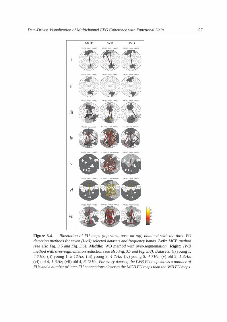
Data-Driven Visualization of Multichannel EEG Coherence with FunctionalUnits 57
MCB WB IWB
i
2 FU(s); 1 sign. conn(s).
1
2
3 FU(s); 3 sign. conn(s).
12
3
2 FU(s); 1 sign. conn(s).
1
3
ii
2 FU(s); 0 sign. conn(s).
1
2
1 FU(s); 0 sign. conn(s).
1
2 FU(s); 0 sign. conn(s).
1
2
iii
6 FU(s); 4 sign. conn(s).
1
2
3
4
5
6
4 FU(s); 4 sign. conn(s).
12
3
4
3 FU(s); 2 sign. conn(s).
2
4
6
iv
5 FU(s); 5 sign. conn(s).
1
23
4 5
10 FU(s); 27 sign. conn(s).
12
34
5
6
7
8
9
10
6 FU(s); 8 sign. conn(s).
5
6
7
8
910
v
1 FU(s); 0 sign. conn(s).
1
6 FU(s); 15 sign. conn(s).
2
3
5
7
8
9
2 FU(s); 1 sign. conn(s).
1
10
vi
2 FU(s); 1 sign. conn(s).
1
2
6 FU(s); 15 sign. conn(s).
12
3
45
6
2 FU(s); 1 sign. conn(s).
3
7
vii
6 FU(s); 4 sign. conn(s).
1
2
3
4
56
10 FU(s); 23 sign. conn(s).
12
3
4
5
6
7
8
912
7 FU(s); 7 sign. conn(s).
3
5
7
8
9
10
12
0.3
0.4
0.5
0.6
0.7
Figure 3.4. Illustration of FU maps (top view, nose on top) obtained with the three FUdetection methods for seven (i-vii ) selected datasets and frequency bands.Left: MCB method(see also Fig. 3.5 and Fig. 3.6).Middle: WB method with over-segmentation.Right: IWBmethod with over-segmentation reduction (see also Fig. 3.7 and Fig. 3.8). Datasets:(i) young 1,4-7Hz; (ii) young 1, 8-12Hz; (iii) young 3, 4-7Hz; (iv) young 5, 4-7Hz; (v) old 2, 1-3Hz;(vi) old 4, 1-3Hz; (vii) old 4, 8-12Hz. For every dataset, the IWB FU map shows a number ofFUs and a number of inter-FU connections closer to the MCB FU maps than the WB FU maps.
58 3.7 Results
method, however, results in 6 FUs completely connected by 15lines and does not (directly)make clear that the used threshold is too low.
vi. Both FUs found with the MCB and the IWB method are identical. The WBmethod hasmore FUs in the same region instead.
vii. The large anterior FUs found with the MCB and the IWB method are identical. The WBmethod has multiple FUs in the same region instead.
In all cases, the number of FUs and their size and locations are highly similar for the MCBFU maps and the corresponding IWB FU maps (Fig. 3.5–3.8). The absolute difference in thenumber of FUs between the WB and the MCB method is on average 1.8 with a maximum dif-ference of five FUs (four occurrences). The same difference between the IWB and the MCB isclearly smaller: 0.9 with a maximum of three FUs difference (two occurrences). Regarding theconnections between FUs, those found with the MCB method are generally also found in thecorresponding IWB FU maps. In particular, connections between a middle anterior and a middleposterior FU are present in the MCB FU map if and only if they arepresent in the correspond-ing IWB FU map, with one exception: for datasetold 5, 21-30Hz, the inter-FU coherence is justabove the threshold for the IWB method, contrary to the MCB method. For datasetsold 2and thefrequencies 1-3Hz, the connection between anterior and posterior regions is explicit in the IWBFU map (Fig. 3.8) and implicit in the MCB FU map (Fig. 3.6: the fact that one large FU con-sists of nearly all vertices implies that most anterior and most posterior vertices are completelyconnected).
3.7.2 Group Analysis
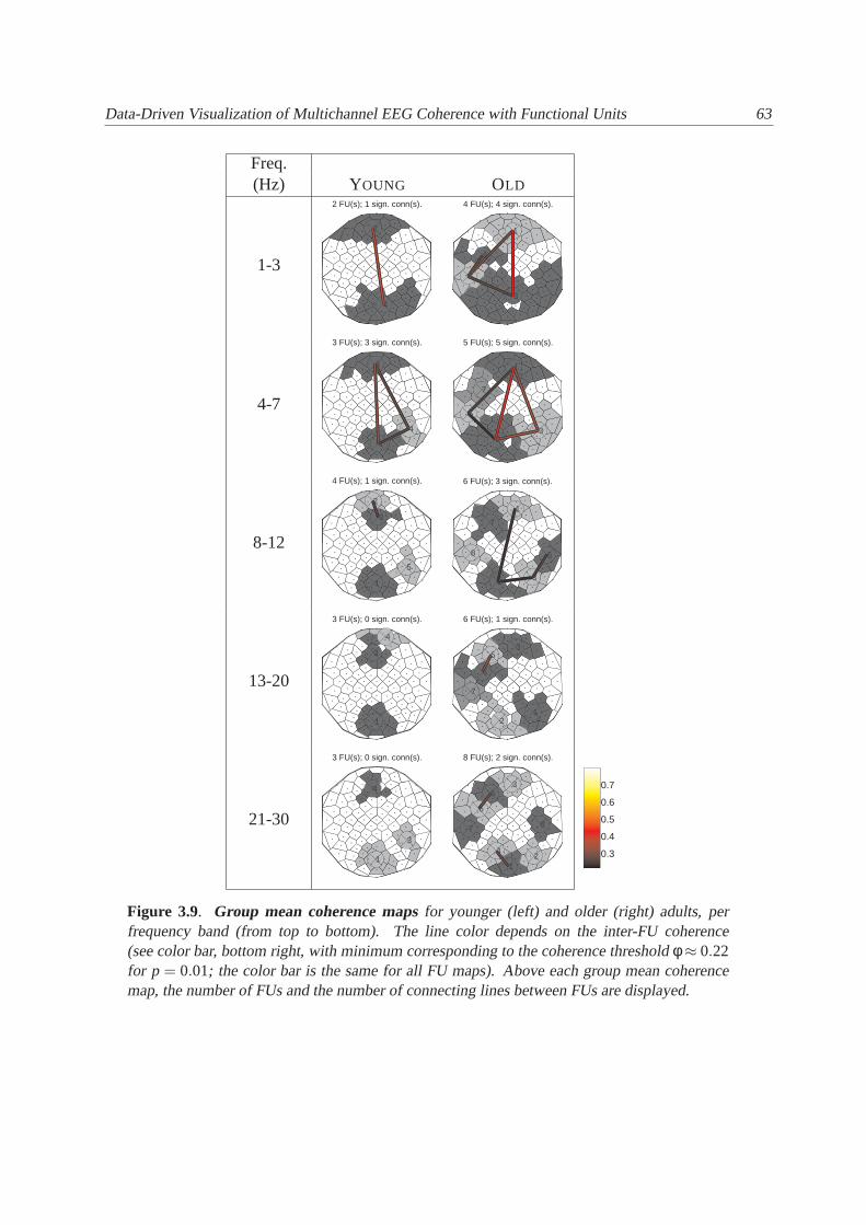
Group mean coherence maps (Fig. 3.9) and group FU size maps (Fig. 3.10) were obtained asextensions of the IWB FU detection method. They are shown for the two groups of younger andolder adults and the five frequency bands.
Individual FU Maps versus Group Mean Coherence Maps
The largest FUs for individual datasets of younger adults (Fig. 3.5, 3.7) are mostly located anteri-orly and posteriorly in the middle. This feature is also preserved in the corresponding group meancoherence maps (Fig. 3.9, left column). FU maps for older adults (Fig. 3.6, 3.8) usually showmore lateral FUs (at the sides of the head), which are preserved in the corresponding group meancoherence maps (Fig. 3.9, right). For both younger and olderadults, the number of FUs usuallydoes not change much across frequency bands in the individual dataset FU maps (Fig. 3.5–3.8,compare rows), as well as in the group mean coherence maps (Fig. 3.9, compare rows). In fourout of five frequency bands, inter-FU connections between a middle anterior and middle poste-rior FU are present in the group mean coherence map (Fig. 3.9)if they are present in the majorityof the individual FU maps in the corresponding frequency bands (Figs. 3.5–3.8). The only ex-ception is the 8-12Hz band, with anterior-posterior connections just above the threshold for amajority of three (out of five) younger adults, and with anterior-posterior connections above the
Data-Driven Visualization of Multichannel EEG Coherence with FunctionalUnits 59
YOUNGFreq. (Hz)
1-3 4-7 8-12 13-20 21-30
1.
2 FU(s); 0 sign. conn(s).
1
2
2 FU(s); 1 sign. conn(s).
1
2
2 FU(s); 0 sign. conn(s).
1
2
2 FU(s); 1 sign. conn(s).
1
2
3 FU(s); 0 sign. conn(s).
1
2
3
2.
2 FU(s); 1 sign. conn(s).
1
2
3 FU(s); 3 sign. conn(s).
1
2
3
3 FU(s); 1 sign. conn(s).
1
2
3
3 FU(s); 1 sign. conn(s).
1
2
3
5 FU(s); 2 sign. conn(s).
12
3
4
5
3.
5 FU(s); 3 sign. conn(s).
1
23
4
5
6 FU(s); 4 sign. conn(s).
1
2
3
4
5
6
5 FU(s); 3 sign. conn(s).
1
2
3
4
5
6 FU(s); 2 sign. conn(s).
1
2
3
4
5
6
5 FU(s); 0 sign. conn(s).
1
2
3
4
5
4.
4 FU(s); 1 sign. conn(s).
1
2
3
4
7 FU(s); 2 sign. conn(s).
1
2
3
4
56
7
6 FU(s); 0 sign. conn(s).
1
2
3
4
5
6
6 FU(s); 0 sign. conn(s).
1
2
3
4
5
6
5 FU(s); 0 sign. conn(s).
1
2
3
4
5
5.
4 FU(s); 6 sign. conn(s).
1
2
3
4
5 FU(s); 5 sign. conn(s).
1
23
4 5
8 FU(s); 4 sign. conn(s).
1
2
3
4
5
6
7
8
5 FU(s); 2 sign. conn(s).
1
2
3
4
5
4 FU(s); 0 sign. conn(s).
1
2
34
0.3
0.4
0.5
0.6
0.7
Figure 3.5. Standard MCB FU maps, younger adults. FU maps (|FU | > 5, p = 0.01)for five younger adults for five frequency bands (1-3, 4-7, 8-12,13-20, 21-30Hz). Each FUis visualized as a set of Voronoi cells with identical gray value, with different gray values foradjacent FUs. White Voronoi cells are part of FUs with|FU | ≤ 5. A line connects FUs if theinter-FU coherence exceeds the significance threshold, with its color depending on the value(see color bar, bottom right, with minimum corresponding to the coherence thresholdφ≈ 0.22for p = 0.01; the color bar is the same for all FU maps). Above each group mean coherencemap, the number of FUs and the number of connecting lines between FUs are displayed.
60 3.7 Results
OLDFreq. (Hz)
1-3 4-7 8-12 13-20 21-30
1.
4 FU(s); 2 sign. conn(s).
1
2
3
4
2 FU(s); 0 sign. conn(s).
1
2
4 FU(s); 1 sign. conn(s).
1
2
3
4
3 FU(s); 0 sign. conn(s).
1
2
3
3 FU(s); 0 sign. conn(s).
1
2
3
2.
1 FU(s); 0 sign. conn(s).
1
5 FU(s); 1 sign. conn(s).
1
2
3
4
5
5 FU(s); 0 sign. conn(s).
1
2
34
5
5 FU(s); 0 sign. conn(s).
1
2
3
4
5
5 FU(s); 0 sign. conn(s).
1
2
3
4
5
3.
5 FU(s); 7 sign. conn(s).
1
2
3 4
5
4 FU(s); 3 sign. conn(s).
1
2
3
4
6 FU(s); 4 sign. conn(s).
1
2
34
5
6
5 FU(s); 4 sign. conn(s).
1
23
4
5
4 FU(s); 1 sign. conn(s).
1
2
3
4
4.
2 FU(s); 1 sign. conn(s).
1
2
3 FU(s); 1 sign. conn(s).
1
2
3
6 FU(s); 4 sign. conn(s).
1
2
3
4
56
8 FU(s); 2 sign. conn(s).
1
2 3
4
5
6
8
9
6 FU(s); 1 sign. conn(s).
1
23
4
5
6
5.
6 FU(s); 4 sign. conn(s).
1
2
3
4
56
8 FU(s); 6 sign. conn(s).
1
2
3
4
56
7
8
9 FU(s); 0 sign. conn(s).
1
2
3
4
56 7
8
9
6 FU(s); 1 sign. conn(s).
1
2
3
45
6
7 FU(s); 0 sign. conn(s).
1
2
34
5
67
0.3
0.4
0.5
0.6
0.7
Figure 3.6. Standard MCB FU maps, older adults. Same parameters as in Fig. 3.5.
threshold for a minority of two (out of five) older adults (with one relatively high value). Thus,generally the common features from the individual FU maps are preserved well in the groupmean coherence maps.
Group Mean Coherence Map: Comparison Between Groups
For all frequencies (1-30Hz), the number of FUs is lower for younger than for older adults inthe corresponding frequency band (Fig. 3.9, compare left with right column). This probably cor-
Data-Driven Visualization of Multichannel EEG Coherence with FunctionalUnits 61
YOUNGFreq. (Hz)
1-3 4-7 8-12 13-20 21-30
1.
2 FU(s); 0 sign. conn(s).
1
4
2 FU(s); 1 sign. conn(s).
1
3
2 FU(s); 0 sign. conn(s).
1
2
2 FU(s); 1 sign. conn(s).
1
2
1 FU(s); 0 sign. conn(s).
1
2.
3 FU(s); 3 sign. conn(s).
2
3
7
2 FU(s); 1 sign. conn(s).
1
8
4 FU(s); 2 sign. conn(s).
3
7
8
9
3 FU(s); 1 sign. conn(s).
3
4
5
4 FU(s); 2 sign. conn(s).
25
6
7
3.
3 FU(s); 3 sign. conn(s).
2
45
3 FU(s); 2 sign. conn(s).
2
4
6
4 FU(s); 3 sign. conn(s).
2
3 4
7
3 FU(s); 1 sign. conn(s).
1
34
3 FU(s); 1 sign. conn(s).
1
3 7
4.
6 FU(s); 6 sign. conn(s).
2
3
4
5
6
7
7 FU(s); 1 sign. conn(s).
1
3
4
56
9
13
4 FU(s); 0 sign. conn(s).
1
2
3
7
4 FU(s); 0 sign. conn(s).
1
2
5
6
4 FU(s); 0 sign. conn(s).
1
3
5
7
5.
5 FU(s); 8 sign. conn(s).
2
56
8 9
6 FU(s); 8 sign. conn(s).
5
6
7
8
910
6 FU(s); 2 sign. conn(s).
2
3
5
6 7
8
5 FU(s); 3 sign. conn(s).
12
3
4
7
3 FU(s); 0 sign. conn(s).
1
3
5
0.3
0.4
0.5
0.6
0.7
Figure 3.7. Novel IWB FU maps, younger adults.Same parameters as in Fig. 3.5
responds to earlier findings (Mauritset al. 2006), indicating more, especially interhemispheric,coherence for older than for younger adults. Similarly, thenumber of white cells (correspondingto electrodes not part of any sufficiently large FU) is largerfor younger than for older adultsin every frequency band, again confirming the presence of more coherence for older than foryounger adults (Mauritset al.2006).
For lower frequencies, there is a connecting line between ananterior and a posterior FUin most group mean coherence maps for younger adults (Fig. 3.9, 1-7Hz) and older adults
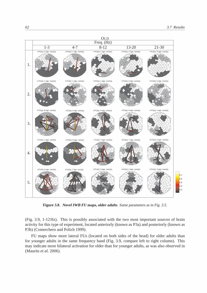
62 3.7 Results
OLDFreq. (Hz)
1-3 4-7 8-12 13-20 21-30
1.
4 FU(s); 2 sign. conn(s).
3
5
6
9
3 FU(s); 1 sign. conn(s).
2
5
6
4 FU(s); 1 sign. conn(s).
3
4
5
6
4 FU(s); 1 sign. conn(s).
2
4
5
6
3 FU(s); 0 sign. conn(s).
23
4
2.
2 FU(s); 1 sign. conn(s).
1
10
5 FU(s); 1 sign. conn(s).
12
8
9
12
5 FU(s); 1 sign. conn(s).
2 3
4
9
11
5 FU(s); 0 sign. conn(s).
12
5
7
8
5 FU(s); 0 sign. conn(s).
2 3
7
8
11
3.
5 FU(s); 8 sign. conn(s).
3
5
6
7
8
5 FU(s); 6 sign. conn(s).
2
4
5
6
7
6 FU(s); 4 sign. conn(s).
1
23
4
5
6
5 FU(s); 4 sign. conn(s).
1
2
3
4
5
4 FU(s); 1 sign. conn(s).
2
3
4
6
4.
2 FU(s); 1 sign. conn(s).
3
7
4 FU(s); 3 sign. conn(s).
2
7
8
11
7 FU(s); 7 sign. conn(s).
3
5
7
8
9
10
12
8 FU(s); 7 sign. conn(s).
1
2
3
4
56
8
9
8 FU(s); 6 sign. conn(s).
1
3
4
5
678
9
5.
6 FU(s); 8 sign. conn(s).
3
56 7
1011
8 FU(s); 7 sign. conn(s).
1
2
3
4
5
6
79
9 FU(s); 3 sign. conn(s).
1
2
3
4
5
67
8
10
6 FU(s); 1 sign. conn(s).
1
2
3
5
6
7
5 FU(s); 3 sign. conn(s).
1
2
3
5
7
0.3
0.4
0.5
0.6
0.7
Figure 3.8. Novel IWB FU maps, older adults. Same parameters as in Fig. 3.5.
(Fig. 3.9, 1-12Hz). This is possibly associated with the twomost important sources of brainactivity for this type of experiment, located anteriorly (known as P3a) and posteriorly (known asP3b) (Comerchero and Polich 1999).
FU maps show more lateral FUs (located on both sides of the head) for older adults thanfor younger adults in the same frequency band (Fig. 3.9, compare left to right column). Thismay indicate more bilateral activation for older than for younger adults, as was also observed in(Mauritset al.2006).
Data-Driven Visualization of Multichannel EEG Coherence with FunctionalUnits 63
Freq.(Hz) YOUNG OLD
1-3
2 FU(s); 1 sign. conn(s).
2
4
4 FU(s); 4 sign. conn(s).
1
3
6
8
4-7
3 FU(s); 3 sign. conn(s).
1
3
4
5 FU(s); 5 sign. conn(s).
1
23
5
7
8-12
4 FU(s); 1 sign. conn(s).
1
2
3
5
6 FU(s); 3 sign. conn(s).
1
2 3
6
7
8
13-20
3 FU(s); 0 sign. conn(s).
1
3
4
6 FU(s); 1 sign. conn(s).
12
35
6
7
21-30
3 FU(s); 0 sign. conn(s).
1
3
4
8 FU(s); 2 sign. conn(s).
12
3
4
5
6
7 8
0.3
0.4
0.5
0.6
0.7
Figure 3.9. Group mean coherence mapsfor younger (left) and older (right) adults, perfrequency band (from top to bottom). The line color depends on the inter-FU coherence(see color bar, bottom right, with minimum corresponding to the coherence thresholdφ≈ 0.22for p = 0.01; the color bar is the same for all FU maps). Above each group mean coherencemap, the number of FUs and the number of connecting lines between FUs are displayed.
64 3.7 Results
Freq.(Hz) YOUNG OLD
1-3
5
10
15
20
25
0
10
20
30
40
4-7
5
10
15
20
5
10
15
20
25
30
35
8-12
0
5
10
15
5
10
15
13-20
0
5
10
15
0
5
10
15
21-30
0
2
4
6
8
10
12
0
2
4
6
8
10
12
Figure 3.10. Group FU size mapsfor younger (left) and older (right) adults, per frequencyband (from top to bottom). The average FU size for each electrode, computed for the five in-dividual FU maps of every group (see Fig. 3.9), is mapped to a gray value(see right bar, withmaximum equal to the maximum average FU size). A lighter cell indicates that the correspond-ing electrode is on average part of larger and more interesting FUs. The gray scale range isadapted per group FU size map, to be able to better distinguish between light and dark regionsin one FU size map.
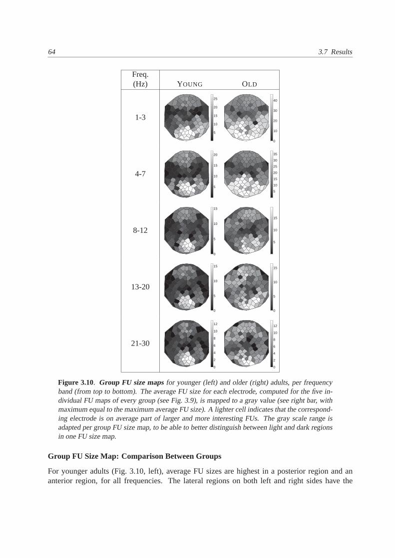
Group FU Size Map: Comparison Between Groups
For younger adults (Fig. 3.10, left), average FU sizes are highest in a posterior region and ananterior region, for all frequencies. The lateral regions on both left and right sides have the

Data-Driven Visualization of Multichannel EEG Coherence with FunctionalUnits 65
lowest average FU size.
Similarly, for older adults (Fig. 3.10, right), the highestaverage FU sizes occur in a posteriorand an anterior region, although for older adults those regions are more widespread than foryounger adults. Whereas the average FU sizes are lower on the sides than in the middle for bothyounger and older adults (Fig. 3.10), the difference between lower and higher average FU sizesis smaller for older than younger adults. This indicates more bilateral activation for older thanyounger adults, in correspondence with (Mauritset al.2006).
Cells for younger adults are generally part of FUs with a loweraverage size than corre-sponding cells for older adults (Fig. 3.10, compare color bars of the left and right column), oncemore confirming the observation of higher coherence for older than younger adults (Mauritsetal. 2006). Moreover, the average FU size decreases with increasing frequency, in agreement withthe presence of simultaneous activity at a more global scalefor lower EEG frequencies and at amore local scale for higher EEG frequencies (Nunezet al.1997).
Comparison of Hypothesis-Driven and Data-Driven Approaches
For the same type of data, a hypothesis-driven subselectionof 12 out of 119 scalp electrodes (Fp1,Fp2, F3, F4, C3, C4, P3, P4, O1, O2, O3, O4; see Fig. 3.1, right) and 15 coherences was made(Maurits et al. 2006). In contrast to this hypothesis-driven approach, FU maps together withgroup mean coherence maps and group FU size maps all contribute to a data-driven selectionof electrodes of interest. In addition to the coherences studied in (Mauritset al. 2006), ourdata-driven results suggest to include left and right temporal electrodes (e.g., T7 and T8), and toinclude both intrahemispheric and interhemispheric connections between anterior and posteriorregions.
3.7.3 Threshold Effect
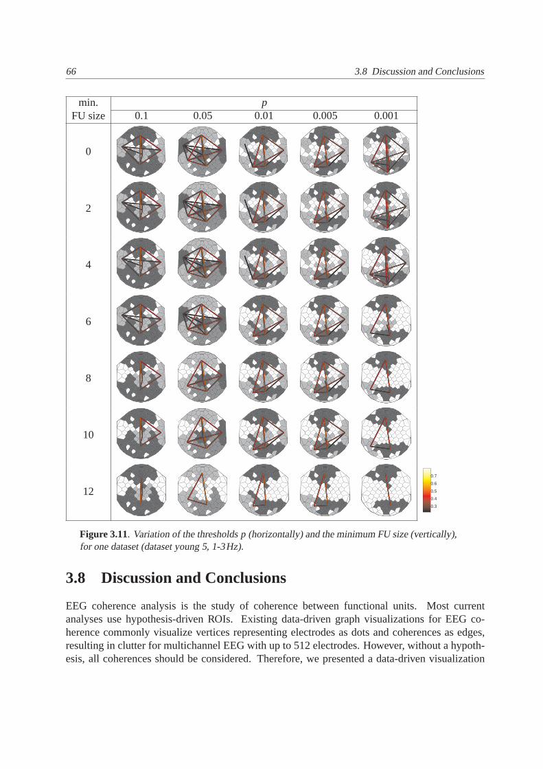
Two thresholds applied in the FU visualization are coherence thresholds. One concerns the initialcoherence graph, the other the inter-FU coherence. Both are chosen to be equal to each other andare related to a valuep (Eqn. 3.1). A third threshold is the minimum FU size.
Threshold variation is illustrated by FU maps for one dataset and one frequency band, vary-ing p and the minimum FU size (Fig. 3.11). Obviously, larger FUs are found for a higherpcorresponding with a lower coherence threshold. For the value p = 0.1, the highest inter-FUcoherence occurs between largest FUs which are located anteriorly and posteriorly. The sameis visible for the valuep = 0.001. Other significant inter-FU coherence appear between smallerFUs located laterally on the left and the right side, for all values ofp.
For other datasets and frequency bands, we have generally observed a similar pattern. Acrossdifferent threshold values, the largest FUs remain in the same regions and the highest inter-FUcoherences remain between FUs in the same regions.
66 3.8 Discussion and Conclusions
min. pFU size 0.1 0.05 0.01 0.005 0.001
0
2
4
6
8
10
12
0.3
0.4
0.5
0.6
0.7
Figure 3.11. Variation of the thresholdsp (horizontally) and the minimum FU size (vertically),for one dataset (dataset young 5, 1-3Hz).
3.8 Discussion and Conclusions
EEG coherence analysis is the study of coherence between functional units. Most currentanalyses use hypothesis-driven ROIs. Existing data-driven graph visualizations for EEG co-herence commonly visualize vertices representing electrodes as dots and coherences as edges,resulting in clutter for multichannel EEG with up to 512 electrodes. However, without a hypoth-esis, all coherences should be considered. Therefore, we presented a data-driven visualization
Data-Driven Visualization of Multichannel EEG Coherence with FunctionalUnits 67
method for multichannel EEG coherence, which strongly reduces clutter and is referred to asfunctional unit (FU) map. An FU is a spatially connected set of electrodes recording pairwisesignificantly coherent signals, represented in the graph bya spatially connected clique. The vi-sualization of an FU is a simplified representation of a spatially connected clique which does notexplicitly visualize all edges within a clique.
We developed three methods to detect FUs. One is the maximal clique based (MCB) method(time complexityO(3n/3), with n the number of vertices) (ten Caatet al.2007d), another is thewatershed based (WB) method designed with an interactive visualization in mind (time com-plexity O(n2 logn)) (ten Caatet al.2007e). Third, the improved watershed based (IWB) method(time complexityO(n2 logn)) merges two spatially neighboring FUs if their union is a cliquein the coherence graph. We did not choose one of the common solutions for over-segmentationwhich uses the concept of dynamics (Grimaud 1992), because dynamics are defined for vertexvalues, whereas the EEG coherence graph has edge values. Moreover, the IWB method mergesFUs during segmentation (and not afterwards, such as with hierarchical watersheds (Schultzetal. 2007)). FU detection with the WB and IWB method (taking about 0.04s and 0.05s, respec-tively) is up to a factor of 100,000 times faster than the MCB method, and makes interactivevisualization of multichannel EEG coherence possible.
Comparing the methods, the greedy WB and IWB methods directly result in uniquely la-beled electrodes contrary to the standard MCB method. Our three methods depend on the samethresholds: one for the initial coherence graph, one for theinter-FU coherence, and one for theminimum FU size. Threshold changes do not have a large effecton the most eminent FUs andinter-FU coherences. The MCB, WB, and IWB methods find FUs in approximately the samelocations, and the inter-FU connections present in the MCB FUmaps are generally also presentin the WB and IWB FU maps. However, the average difference between the WB and the MCBmethod regarding the number of FUs is 1.8 (for our parameters). The same difference betweenthe IWB and the MCB method has decreased to 0.9, for the case study that was presented.
Additionally, as an alternative to hypothesis-driven group analysis methods for multichannelEEG coherence, we proposed two novel data-driven group mapsfor visual group analysis. Theyare both extensions of the efficient IWB FU detection method. One is a group mean coherencemap, which is a data-driven FU map based on the group mean coherence. The other is a groupFU size map, showing for each electrode the average FU size across a collection of individualFU maps. Both novel group maps represent common elements froma set of individual FU maps.
Because conventional data-driven multichannel EEG coherence analysis is cumbersome,comparable conventional findings are rare. Nevertheless several conventional findings are con-firmed by observations in the new data-driven visualizations. (a) Coherence is lower for youngerthan older adults (Mauritset al. 2006). Accordingly, the number of FUs in group mean coher-ence maps is lower for younger than for older adults for 1-30Hz, group mean coherence mapsshow a larger number of white cells not part of any sufficiently large FU for younger adults thanolder adults, and group FU size maps show larger average FU sizes for older than for youngeradults.(b) Older adults have more bilateral activation than younger adults (Mauritset al.2006).In accordance, FU maps and group mean coherence maps displaymore FUs in lateral regions forolder than younger adults, whereas group FU size maps show that the average FU size is gen-erally higher for older than for younger adults and that the difference between lower and higher
68 3.8 Discussion and Conclusions
average FU sizes is smaller for older than younger adults.(c) There is simultaneous activity at amore global scale for lower EEG frequencies and at a more local scale for higher EEG frequen-cies (Nunezet al. 1997). In agreement, group FU size maps indicate that the average FU sizedecreases with increasing frequency.(d) The two most important sources of brain activity for thistype of data are located anteriorly (known as P3a) and posteriorly (known as P3b) (Comercheroand Polich 1999). Accordingly, FU maps and group mean coherence maps show connectionsbetween anterior and posterior FUs for lower frequencies.
Thus, the detection of data-driven ROIs for multichannel EEG coherence on the basis of theIWB method results in similar information as the MCB method, and this information is foundto agree with conventional findings. Also, the two new data-driven group maps, referred to asgroup mean coherence map and group FU size map, yield resultsin accordance with conven-tional findings. Yet, our results suggest to expand an earlier selection of hypothesis-driven ROIs(Mauritset al. 2006) with additional data-driven ROIs. This demonstratesthe usefulness of theIWB FU map, and both new data-driven group maps.
FU maps, group mean coherence maps, and group FU size maps allcontribute to a data-driven subselection of electrodes of interest (EOIs): the number of EOIs, their location, and theirregion of influence can be derived directly from the combination of FU maps, group mean co-herence maps, and group FU size maps. In other words, the novel IWB method together withthe two new group maps make a data-driven subselection of theavailable electrophysiologicalsignals possible. This can be used as a data-driven startingpoint for conventional quantitativegroup analysis. Our methods are currently applied to a multichannel EEG coherence study ofmental fatigue (ten Caatet al.2007a) by researchers from the Department of Experimental Psy-chology of the University of Groningen. In this study, the ROIs are obtained in a data-drivenway since no strong hypotheses can be formulated based on existing evidence. Our approachovercomes the severe limitations of conventional hypothesis-driven methods and takes full ad-vantage of all the available recordings. The presented visualization of (group) FU maps providesa very economical data summary of extensive experimental results, which otherwise would bevery difficult and time-consuming to assess. Initial responses from the psychologists using ourvisualization methods are very favorable.
The IWB method will be available inFUmaplabonhttp://www.rug.nl/informatica/onderzoek/programmas/svcg/demos .


![Visualization and Exploration of Multichannel EEG ... - rug.nl · bibliography [8]F. Beck, M. Burch, S. Diehl, and D. Weiskopf. The State of the Art in Visualizing Dynamic Graphs.](https://static.fdocuments.net/doc/165x107/5f7ddfa7b5775d0ed06e16fc/visualization-and-exploration-of-multichannel-eeg-rugnl-bibliography-8f.jpg)