UNIVERSIDAD SAN FRANCISCO DE QUITO USFQ Colegio de Posgrados
UNIVERSIDAD SAN FRANCISCO DE QUITO USFQ
Colegio de Ciencias e Ingeniería
Diseño del sistema de refrigeración para la caja lectora del detector de partículas tipo hadrón
. Proyecto de Investigación
David Alejandro Jaramillo Bazurto
Ingeniería Mecánica
Trabajo de titulación presentado como requisito para la obtención del título de
Ingeniero Mecánico
Quito, 10 de mayo 2019
UNIVERSIDAD SAN FRANCISCO DE QUITO USFQ
Colegio de Ciencias e Ingenierías
HOJA DE CALIFICACIÓN
DE TRABAJO DE TITULACIÓN
Diseño del sistema de refrigeración para la caja lectora del detector de partículas tipo hadrón
David Alejandro Jaramillo Bazurto
Calificación:
Nombre del profesor, Título académico: David Escudero Ph.D.
Firma del profesor: ____________________________
Quito, 10 de mayo 2019
2
Derechos de Autor
Por medio del presente documento certifico que he leído todas las Políticas y Manuales
de la Universidad San Francisco de Quito USFQ, incluyendo la Política de Propiedad
Intelectual USFQ, y estoy de acuerdo con su contenido, por lo que los derechos de propiedad
intelectual del presente trabajo quedan sujetos a lo dispuesto en esas Políticas.
Asimismo, autorizo a la USFQ para que realice la digitalización y publicación de este
trabajo en el repositorio virtual, de conformidad a lo dispuesto en el Art. 144 de la Ley Orgánica
de Educación Superior.
Firma del estudiante: _______________________________________ Nombres y apellidos: David Alejandro Jaramillo Bazurto Código: 00117002 Cédula de Identidad: 1716358492 Lugar y fecha: Quito, 10 de mayo de 2019
3
DEDICATORIA
Me gustaría agradecer en estas líneas la ayuda que muchas personas y colegas me han
prestado durante el proceso de investigación y redacción de este trabajo. En primer lugar,
quisiera agradecer a mi familia, especialmente a mis padres que me han ayudado y apoyado
en todo mi producto, a mi tutor, David Escudero, por haberme orientado en todos los
momentos que necesité sus consejos.
Así mismo, deseo expresar mi reconocimiento a la Universidad y a sus profesores por todas
las atenciones e información brindada a lo largo de esta indagación.
Finalmente, a mis amigos. Con todos los que compartí́ dentro y fuera de las aulas. Aquellos
amigos del cole, que se convierten en amigos de vida y aquellos que formaron parte de la
carrera universitaria y quienes serán mis colegas, gracias por todo su apoyo y diversión.
4
ABSTRACT
This project presents a development upgrade for the cooling system of the Readout Module Box (RBx) of the Hadron Calorimeter Detector (HCAL) from the LHC collider. The Compact Muon Solenoid (CMS) experiment will have a better performance if the HCAL electronics are working at the right conditions. One of the suitable options for doing this is by removing the heat from the front end electronics (FEE) located in the RBx compartment using water as a cooling fluid through cooper lines, however the current design is not cooling the electronics effectively, and thus a new design is proposed to cool the system. First, an analytical analysis with the fundamentals of heat transfer mechanism, thermodynamics and fluid mechanics is performed to determine the heat transfer area and then the length of the cooper tube. Then a fluid mechanics analysis to overview the pressure losses in the tube and momentum conservation effect by bends. Also, computational simulations were carried out using COMSOL Multiphysics software to observe the thermal behavior of the RBX using three types of arrangements of cooper lines on the floor of the RBx. The new distribution designs of the copper lines of the refrigeration system reduce the temperature of the RBx in approximately 10°C, improving the performance of the electronics.
Key words: RBx, cooling system, heat dissipated

5
RESUMEN
El presente proyecto es un desarrollo de mejora para el sistema de refrigeración de la caja lectora del detector de partículas tipo hadrón del largo colisionado de partículas. El experimento del solenoide compacto de muones tendrá un mejor rendimiento si el detector de partículas tipo hadrón trabaja en las condiciones correctas. Una de las opciones adecuadas es remover el calor de la caja electrónica frontal ubicada en el compartimento de la caja lectora, mediante el uso de agua como fluido de refrigeración por medio de tuberías de cobre. Sin embargo, el diseño actúa no está enfriando la electrónica eficientemente, por lo que un nuevo diseño es propuesto para enfriar el sistema. En primera instancia, un análisis analítico con los fundamentos de transferencia de calor, termodinámica y mecánica de fluidos es realizado para determinar el área de transferencia de calor y así la longitud de la tubería de cobre. Así también mediante el análisis de mecánica de fluidos se determina las pérdidas de presión en la tubería y la conservación del momento por efecto de los dobleces. Además, simulaciones computacionales fueron llevadas a cabo usando del software COMSOL Multiphysics para observar el comportamiento térmico de la caja lectora usando tres tipos de arreglos de tubería en el piso de la caja lectora. Como resultado, por el método de criterio de ponderados se seleccionó los diseños 1 & 2 para la fase preliminar de este proyecto. La nueva distribución de los diseños de las tuberías de cobre del sistema de refrigeración reduce la temperatura de la caja lectora en aproximadamente 10°C, mejorando el rendimiento de la electrónica. Palabras claves: Caja lectora, sistema de refrigeración, calor disipado
6
INDEX
Dedicatoria ................................................................................................................................. 3 1. Introduction ...................................................................................................................... 13 2. Methodology .................................................................................................................... 22
2.1 Analytical Design ........................................................................................................... 22 2.1.1 Fundamentals of heat transfer. ................................................................................ 22 2.1.2 Fundamentals of fluid mechanics. .......................................................................... 27 2.1.3 Conjugate Heat Transfer: Internal Flow. ................................................................ 29 2.1.4 Fundamentals applied to the system. ...................................................................... 32
2.2 CFD Analysis ................................................................................................................. 38 2.2.1 Comsol Multiphysics Overview. ............................................................................ 38 2.2.2 System design and analysis ..................................................................................... 45
3. RESULTS AND DISCUSSION ...................................................................................... 60 3.1 Mathematical Results ..................................................................................................... 60
3.1.1 Temperature distribution. ........................................................................................ 60 3.1.2 Pipe friction losses. ................................................................................................. 62
3.2 Tube layout results ......................................................................................................... 63 3.3 Simulation Results.......................................................................................................... 65
3.3.1 Qualitative results. .................................................................................................. 65 3.3.2 Quantitative Results. ............................................................................................... 72
4. CONCLUSION AND RECOMMENDATIONS ............................................................... 76 5. FUTURE WORK ............................................................................................................. 77 6. REFERENCES ................................................................................................................ 79 7. APPENDIX ...................................................................................................................... 81
7.1 APPENDIX A ................................................................................................................ 81 7.2 Appendix B .................................................................................................................... 83 7.3 Appendix C .................................................................................................................... 84
Script C.1. Octave script for design proposal 1 ............................................................... 84 Script C.2. Octave script for design proposal 2 ............................................................... 85 Script C.3. Octave script for design proposal 3 ............................................................... 86
7.4 Appendix D .................................................................................................................... 87

7
Acronyms
LHC Large Hadron Collider CMS Compact Muon Solenoid HCAL Hadron Calorimeter HB Hadron Barrel HF Hadron Forward HE Hadron Endcap HO Hadron Outward RBx Readout box FEE Front-End Electronics RM Readout Module QIE Charge Integrator Encoder card ODU Optical Decoder Unit HPD Hybrid Photodiode SiPM Silicon Photomultiplier LS2 Long shutdown 2 OD Outside diameter ID Inside diameter TDR Technical Design Report BC Boundary Condition
8
Nomenclature
𝑞𝑞 heat dissipated 𝑞𝑞𝑥𝑥 heat dissipated in the x direction T Temperature
Tm mean temperature Tin temperature at the inlet Tout temperature at the outlet Dt differential difference of temperature UA Overall heat transfer coefficient 𝑇𝑇1 Temperature at point 1 𝑇𝑇2 Temperature at point 2 𝑞𝑞´´𝑥𝑥 Heat flux 𝛥𝛥𝑇𝑇𝑐𝑐𝑐𝑐 Delta convection temperature 𝛥𝛥𝑇𝑇𝑈𝑈𝑈𝑈 Delta overall heat transfer coefficient 𝑇𝑇𝑠𝑠 Surface temperature 𝑇𝑇∞ Fluid temperature 𝑞𝑞´´𝑥𝑥 Heat flux 𝐸𝐸𝑖𝑖𝑖𝑖 Inside energy 𝐸𝐸𝑜𝑜𝑜𝑜𝑜𝑜 Outside energy 𝐸𝐸𝑔𝑔𝑔𝑔𝑖𝑖 Energy generated 𝐸𝐸𝑠𝑠𝑜𝑜 Storage energy 𝛥𝛥𝑇𝑇𝐼𝐼𝐼𝐼 Temperature difference internal energy 𝑇𝑇𝑄𝑄𝐼𝐼𝐼𝐼 QIE card temperature 𝑇𝑇𝑀𝑀 Module temperature 𝑇𝑇𝑅𝑅𝑅𝑅𝑅𝑅 RBx outside wall temperature �̇�𝑚 mass flow rate ℎ𝐿𝐿 Pressure losses ℎ𝑓𝑓 Major losses ℎ𝑚𝑚 Minor losses 𝑢𝑢 Velocity of fluid F Friction factor V Fluid velocity 𝑣𝑣1 Velocity specified at point 1 𝑣𝑣2 Velocity specified at point 2 𝑃𝑃1 Pressure specified at point 1 𝑃𝑃2 Pressure specified at point 2 𝑍𝑍1 Height specified at point 1 𝑍𝑍2 Height specified at point 2 𝑐𝑐𝑝𝑝 specific heat 𝜌𝜌 density of fluid µ kinematic viscosity K thermal conductivity 𝜀𝜀 Rugosity material 𝐻𝐻 Convection heat transfer coefficient ℎ Mean heat transfer coefficient
9
𝑁𝑁𝑢𝑢 Nusselt number 𝑁𝑁𝑢𝑢 Mean Nusselt number Pr Prandlt number Re Reynolds number 𝑅𝑅𝑅𝑅𝐷𝐷 Reynolds number based on the diameter of
the tube 𝐴𝐴 heat transfer area 𝐷𝐷 Diameter of tube
ID (D) Inner diameter OD Outside diameter Dx Differential of a x segment Δx Delta x L Length of tube 𝐴𝐴𝑜𝑜 Tube area 𝐴𝐴𝑝𝑝 Plain area ΔV Voltage difference
I Current R Resistance 𝑅𝑅𝑜𝑜 Thermal resistance ∑𝑅𝑅𝑜𝑜 Sum of resistances 𝑅𝑅𝑐𝑐𝑐𝑐 Conduction resistance 𝑅𝑅𝑐𝑐𝑐𝑐 Convection resistance 𝑅𝑅𝑜𝑜𝑜𝑜𝑜𝑜 Total resistance 𝑅𝑅𝑜𝑜𝑜𝑜𝑜𝑜 Sum of total resistances
d Differential

10
LIST OF FIGURES
Figure 1. CMS Overview (INSTITUTE OF PHYSICS PUBLISHING AND SISSA, 2008) . 13 Figure 2. HCAL Sections Overview (Ruchti, 2001) ................................................................ 14 Figure 3. Isometric view of a complete half barrel of the HB HCAL (Barney, 2003) ............ 14 Figure 4. Isometric view of the HB wedges, showing the hermetic design of the scintillator tiles (INSTITUTE OF PHYSICS PUBLISHING AND SISSA, 2008) ................................... 15 Figure 5. An r-z schematic drawing of quarter of the HCAL section showing the RBx location ( CERN Geneva The LHC Experiments Committee, 1997) ...................................... 16 Figure 6. Isometric view of a wedge mockup showing the RBx location (Ruchti, 2001) ....... 16 Figure 7. Drawing of a Readout box and its components (Schmidt, 2018) ............................ 17 Figure 8. Drawing of a RM without covers (Schmidt, 2018) .................................................. 18 Figure 9. Detail of copper tubes on the shell of the RBx (Schmidt, 2018) .............................. 20 Figure 10. Temperature distribution of electronics in the RBx (Schmidt, 2018) .................... 20 Figure 11. Illustration conduction mode ................................................................................. 23 Figure 12. Illustration convection mode .................................................................................. 24 Figure 13. Thermal resistance analogy ................................................................................... 26 Figure 14. Boundary layers. a) Velocity boundary layer. b) Thermal boundary layer [Incropera, 2011]...................................................................................................................... 30 Figure 15. Thermal energy ilustration ..................................................................................... 32 Figure 16. Heat load from electronics in the RBx (Schmidt, 2018) ........................................ 33 Figure 17. Graphical model for the mathematical analysis ..................................................... 34 Figure 18. Conservation of heat in the system ........................................................................ 35 Figure 19. Temperature vs position system graph ................................................................... 36 Figure 20. Comsol Multiphysics Overview (Wollblad, 2017) ................................................ 38 Figure 21. Comsol steps setup ................................................................................................. 39 Figure 22. Pattern proposals for tube floor. a) Proposal 1. b) Proposal 2 (CAE ASSOCIATES, 2009). c) Proposal 3 (Yang, 2009)................................................................. 46 Figure 23. Tube variables description ...................................................................................... 46 Figure 24. Layout proposal design 1........................................................................................ 50 Figure 25. Layout proposal design 2........................................................................................ 51 Figure 26. Layout proposal design 3........................................................................................ 51 Figure 27. Comsol model ......................................................................................................... 52 Figure 28. Geometry setup for Comsol model......................................................................... 53 Figure 29. Material setup for Comsol model ........................................................................... 54 Figure 30. Heat transfer in solids module setup for Comsol model ........................................ 55 Figure 31. Non isothermal module fluid flow setup for Comsol model .................................. 56 Figure 32. Non isothermal module heat transfer setup for Comsol model .............................. 57 Figure 33. Mesh setup for Comsol model ................................................................................ 58 Figure 34. Study setup for Comsol model ............................................................................... 59 Figure 35. Temperature function graph ................................................................................... 61 Figure 36. Relationship between cooling area and temperature .............................................. 62 Figure 37. Pressure change in function of length and number of lengths................................ 63 Figure 38. Proposal design 1 result .......................................................................................... 64 Figure 39. Proposal design 2 result .......................................................................................... 64 Figure 40. Proposal design 3 result .......................................................................................... 64 Figure 41. Initial temperature distribution of the system at t = 30 [min]................................. 65 Figure 42. Temperature distributon system of the present design at t = 35 [min] .................. 66

11
Figure 43. Temperature distribution system at t = 35 [min] a). Design 1................................ 67 b) Design 2. c) Design 3. ........................................................................................................ 67 Figure 44. Heat flux distribution at t = 35[min]. a). Design 1 ................................................. 68 b) Design 2. c) Design 3. ........................................................................................................ 68 Figure 45. Floor temperature distribution at t = 35[min]. a). Design 1 ................................... 70 b) Design 2. c) Design 3. ........................................................................................................ 70 Figure 46. Module 1 temperature distribution at t = 35[min]. a). Design 1 ............................ 71 b) Design 2. c) Design 3. ........................................................................................................ 71 Figure 47. Transient study of water at t = 35[min]. ................................................................. 72 Figure 48. Transient study of module 1 from t = 30 [min] to t = 35 [min]. ............................. 73 Figure 49. Transient study of floor from t = 30 [min] to t = 35 [min]. .................................... 73 Figure 50. Experimental setup of the prototype cooling system. ............................................ 77

12
LIST OF TABLES
Table 1. Known parameters of the RBx (Schmidt, 2018) ........................................................ 33 Table 2. Heat transfer analysis assumptions ............................................................................ 34 Table 3. Comsol steps description ........................................................................................... 39 Table 4. Common nodes or features in each Comsol step ....................................................... 40 Table 5. Common nodes or features for heat transfer in solids module .................................. 41 Table 6. Common nodes or features for non-isothermal flow module in heat transfer ........... 43 Table 7. Common nodes or features for non-isothermal flow module in fluid flow ............... 44 Table 8. Specification and values for the general variables of the design proposals............... 49 Table 9. Detail of the fill and modified variables of the design proposals .............................. 49 Table 10. Fluid properties results............................................................................................. 60 Table 11. Length per design..................................................................................................... 65 Table 12. Centralized weight method ...................................................................................... 74 Table 13. Experimental Setup Proposed Budget ..................................................................... 78
13
1. INTRODUCTION
The curiosity of humanity to understand the origin of matter has deliver results such as the
Higgs Boson or the God´s particle. This investigation was concluded by using the LHC from
CERN laboratories. The LHC particle accelerator is located at Geneva, Switzerland and has a
27 km diameter tunnel, installed 100 meters underground. The main motivation for the
development of the LHC project, is to probe the structure of matter and the forces that control
it by yielding collision of two protons. Furthermore, the observation of these particles could
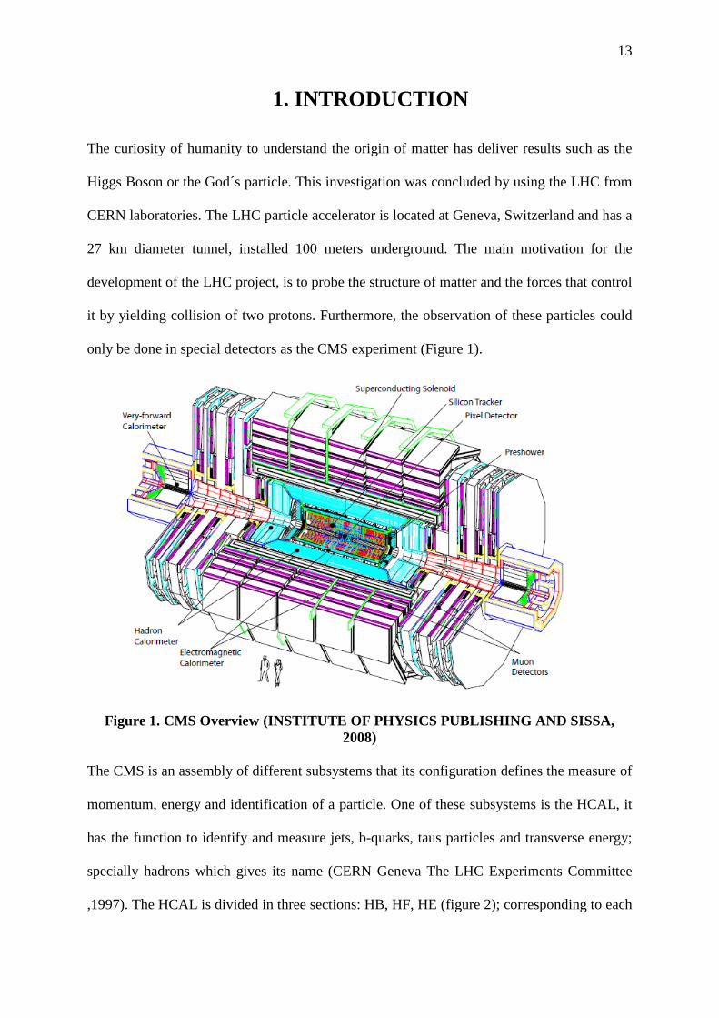
only be done in special detectors as the CMS experiment (Figure 1).
Figure 1. CMS Overview (INSTITUTE OF PHYSICS PUBLISHING AND SISSA, 2008)
The CMS is an assembly of different subsystems that its configuration defines the measure of
momentum, energy and identification of a particle. One of these subsystems is the HCAL, it
has the function to identify and measure jets, b-quarks, taus particles and transverse energy;
specially hadrons which gives its name (CERN Geneva The LHC Experiments Committee
,1997). The HCAL is divided in three sections: HB, HF, HE (figure 2); corresponding to each

14
part specific features to distinguish the type of particles they can detect. The HB is composed
of two half barrels of 18 wedges per barrel, sums up to 36 wedges (figure 3). A wedge is a
compartment which structure is configure as a sandwich of brass plates in the inside and
stainless-steel plates on the outside faces (figure 4). Moreover, the HB houses the front-end
electronics and the back-end electronics which are responsible for the data transmission of the
proton-proton collisions events in the CMS (The Phase-2 Upgrade of the CMS Barrel
Calorimeters TDR, 2017).
Figure 2. HCAL Sections Overview (Ruchti, 2001)
Figure 3. Isometric view of a complete half barrel of the HB HCAL (Barney, 2003)

15
Figure 4. Isometric view of the HB wedges, showing the hermetic design of the scintillator tiles (INSTITUTE OF PHYSICS PUBLISHING AND SISSA, 2008)
Furthermore, the HCAL integrates an optical system that converts the energy from the
collisions of the proton-proton particles to a digital signal. The optical system started with the
collection and storage of the energy in the brass plates from the collisions. Then, the light is
emitted by the scintillator tiles which are special thin plates that its material reacts to energy
and convert it to light; they are visible by using wavelength shifting fibers which are embedded
in the tiles. The energy is further transported in special fibers called optical fibers to the front-
end electronics. Here, the light is detected by a photodetector which account to convert the
optical signal (light) to an analog signal. At last, all the data process in the optical system is
sent to a room outside from the CMS.
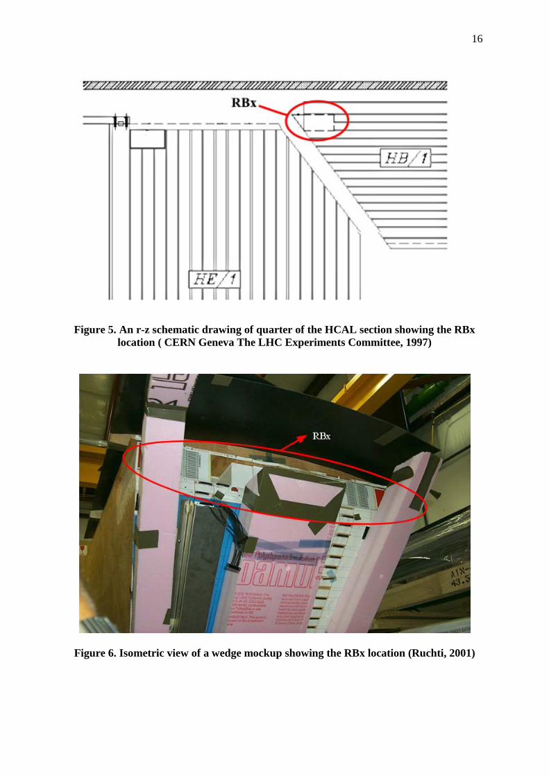
The FEE lies in each wedge, specifically in a component called RBx; that seems as a
rectangular box. Each wedge has a cutoff in its back part to house the RBx.; Figures 5 and 6
detail the location of the RBx in the HCAL.
16
Figure 5. An r-z schematic drawing of quarter of the HCAL section showing the RBx location ( CERN Geneva The LHC Experiments Committee, 1997)
Figure 6. Isometric view of a wedge mockup showing the RBx location (Ruchti, 2001)
17
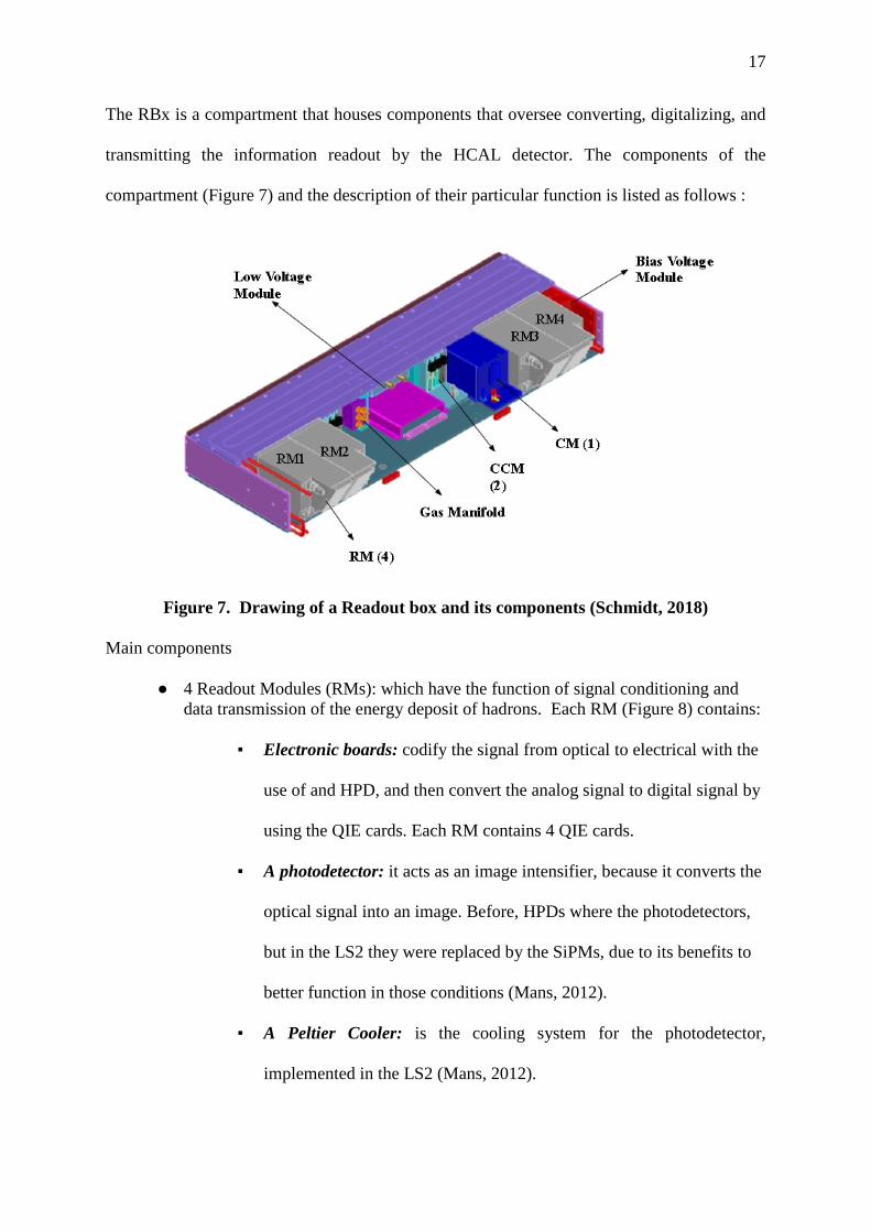
The RBx is a compartment that houses components that oversee converting, digitalizing, and
transmitting the information readout by the HCAL detector. The components of the
compartment (Figure 7) and the description of their particular function is listed as follows :
Figure 7. Drawing of a Readout box and its components (Schmidt, 2018)
Main components
● 4 Readout Modules (RMs): which have the function of signal conditioning and data transmission of the energy deposit of hadrons. Each RM (Figure 8) contains:
▪ Electronic boards: codify the signal from optical to electrical with the
use of and HPD, and then convert the analog signal to digital signal by
using the QIE cards. Each RM contains 4 QIE cards.
▪ A photodetector: it acts as an image intensifier, because it converts the
optical signal into an image. Before, HPDs where the photodetectors,
but in the LS2 they were replaced by the SiPMs, due to its benefits to
better function in those conditions (Mans, 2012).
▪ A Peltier Cooler: is the cooling system for the photodetector,
implemented in the LS2 (Mans, 2012).

18
▪ An ODU: is the receiver of the optical fibers that comes from the
scintillator tiles.
● 1 Calibration Module (CM): it generates a led pulse through a laser pulse for calibration.
● 1 Clock and Control Module (CCM): oversees controlling the other modules. Secondary components
● Bias voltage module: regulates the required voltage to the photodetector.
● Low voltage module: regulates the required voltage to the FEE.
Figure 8. Drawing of a RM without covers (Schmidt, 2018) The LHC is undergoing over a series of upgrades to optimize the detection and storage of the
collisions. In the phase 2 such changes as the integration of the peliter cooler and modifications
of the modules of the RBx has be done. Nowadays, to a better performance the cooling system
has to be upgrade as well, which is the main objective of this senior thesis (Butler, 2011).
19
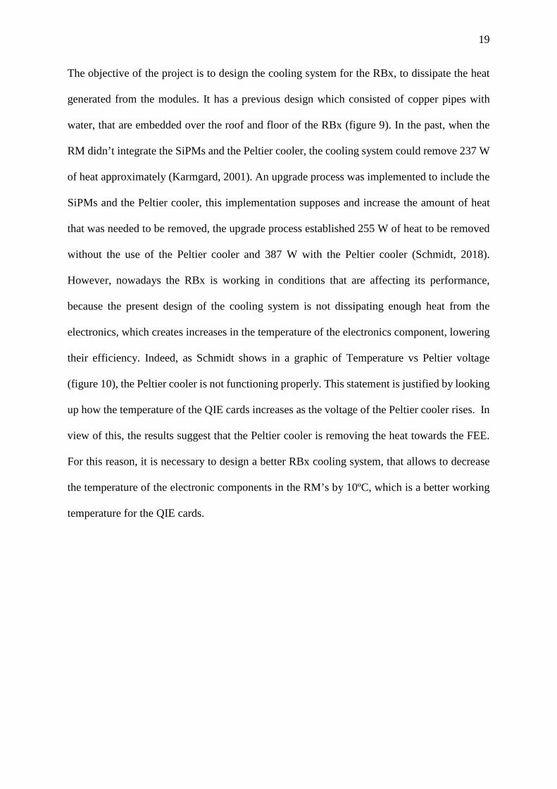
The objective of the project is to design the cooling system for the RBx, to dissipate the heat
generated from the modules. It has a previous design which consisted of copper pipes with
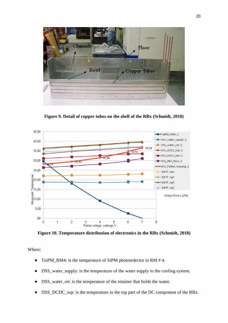
water, that are embedded over the roof and floor of the RBx (figure 9). In the past, when the
RM didn’t integrate the SiPMs and the Peltier cooler, the cooling system could remove 237 W
of heat approximately (Karmgard, 2001). An upgrade process was implemented to include the
SiPMs and the Peltier cooler, this implementation supposes and increase the amount of heat
that was needed to be removed, the upgrade process established 255 W of heat to be removed
without the use of the Peltier cooler and 387 W with the Peltier cooler (Schmidt, 2018).
However, nowadays the RBx is working in conditions that are affecting its performance,
because the present design of the cooling system is not dissipating enough heat from the
electronics, which creates increases in the temperature of the electronics component, lowering
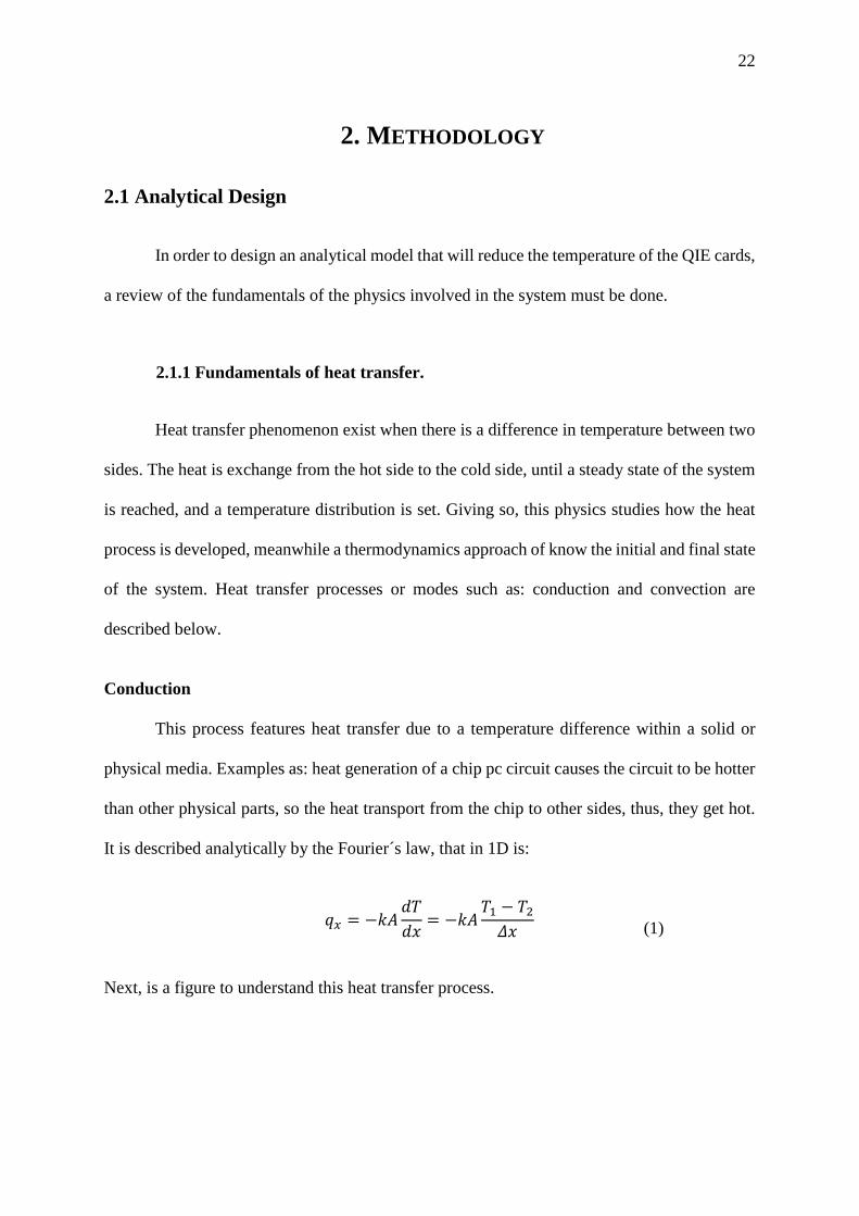
their efficiency. Indeed, as Schmidt shows in a graphic of Temperature vs Peltier voltage
(figure 10), the Peltier cooler is not functioning properly. This statement is justified by looking
up how the temperature of the QIE cards increases as the voltage of the Peltier cooler rises. In
view of this, the results suggest that the Peltier cooler is removing the heat towards the FEE.
For this reason, it is necessary to design a better RBx cooling system, that allows to decrease
the temperature of the electronic components in the RM’s by 10ºC, which is a better working
temperature for the QIE cards.
20
Figure 9. Detail of copper tubes on the shell of the RBx (Schmidt, 2018)
Figure 10. Temperature distribution of electronics in the RBx (Schmidt, 2018)
Where:
● TsiPM_RM4: is the temperature of SiPM phototedector in RM # 4.
● DSS_water_supply: is the temperature of the water supply to the cooling system.
● DSS_water_ret: is the temperature of the retainer that holds the water.
● DSS_DCDC_top: is the temperature in the top part of the DC component of the RBx.

21
● DSS_DCDC_bot: is the temperature in the bottom part of the DC component of the
RBx.
● DSS_RBx_floor: is the temperature of the floor of the RBx
● DSS_Peltier housing: is the temperature of the box that contains inside the peltier.
● QIE: is the temperature of the QIE card. The goal of this project is to design a new distribution layout for the copper tubes on the floor
of the Rbx. Therefore, it will help dissipate the heat produced by the electronics in the RBx
and reduce the temperature of these components.
22
2. METHODOLOGY
2.1 Analytical Design
In order to design an analytical model that will reduce the temperature of the QIE cards,
a review of the fundamentals of the physics involved in the system must be done.
2.1.1 Fundamentals of heat transfer.
Heat transfer phenomenon exist when there is a difference in temperature between two
sides. The heat is exchange from the hot side to the cold side, until a steady state of the system
is reached, and a temperature distribution is set. Giving so, this physics studies how the heat
process is developed, meanwhile a thermodynamics approach of know the initial and final state
of the system. Heat transfer processes or modes such as: conduction and convection are
described below.
Conduction
This process features heat transfer due to a temperature difference within a solid or
physical media. Examples as: heat generation of a chip pc circuit causes the circuit to be hotter
than other physical parts, so the heat transport from the chip to other sides, thus, they get hot.
It is described analytically by the Fourier´s law, that in 1D is:
𝑞𝑞𝑥𝑥 = −𝑘𝑘𝐴𝐴𝑑𝑑𝑇𝑇𝑑𝑑𝑑𝑑
= −𝑘𝑘𝐴𝐴𝑇𝑇1 − 𝑇𝑇2𝛥𝛥𝑑𝑑
(1)
Next, is a figure to understand this heat transfer process.

23
Figure 11. Illustration conduction mode
In addition, sometimes is useful an expression to indicate the direction of heat, as a vector.
This expression namely heat flux is function of the area and heat rate. Its expression in the x
direction is:
𝑞𝑞´´𝑥𝑥 =
𝑞𝑞𝑥𝑥𝐴𝐴
(2)
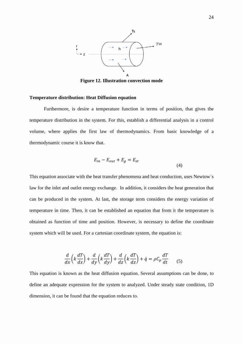
Convection
This process features heat transfer between the temperature difference of a solid and a
fluid. Typical examples as the experiment to take out the hand of a car in movement, gives the
sensation that the hand feel cold due to the convection process that acts around it. As the
example, sometimes the solid could be in movement or the opposite could also occur, when
the fluid is in movement. This mode is described by Newton´s law of cooling, which is:
𝑞𝑞 = ℎ𝐴𝐴𝛥𝛥𝑇𝑇𝑐𝑐𝑐𝑐 = ℎ𝐴𝐴(𝑇𝑇𝑆𝑆 − 𝑇𝑇∞)
(3)
Where the 𝐴𝐴 = 𝜋𝜋(𝐼𝐼𝐷𝐷)𝐿𝐿. Like in conduction, a figure is used to understand better the convection process.
24
Figure 12. Illustration convection mode
Temperature distribution: Heat Diffusion equation
Furthermore, is desire a temperature function in terms of position, that gives the
temperature distribution in the system. For this, establish a differential analysis in a control
volume, where applies the first law of thermodynamics. From basic knowledge of a
thermodynamic course it is know that.
𝐸𝐸𝑖𝑖𝑖𝑖 − 𝐸𝐸𝑜𝑜𝑜𝑜𝑜𝑜 + 𝐸𝐸𝑔𝑔 = 𝐸𝐸𝑠𝑠𝑜𝑜
(4) This equation associate with the heat transfer phenomena and heat conduction, uses Newtow´s
law for the inlet and outlet energy exchange. In addition, it considers the heat generation that
can be produced in the system. At last, the storage term considers the energy variation of
temperature in time. Then, it can be established an equation that from it the temperature is
obtained as function of time and position. However, is necessary to define the coordinate
system which will be used. For a cartesian coordinate system, the equation is:
𝑑𝑑𝑑𝑑𝑑𝑑
�𝑘𝑘𝑑𝑑𝑇𝑇𝑑𝑑𝑑𝑑� +
𝑑𝑑𝑑𝑑𝑑𝑑
�𝑘𝑘𝑑𝑑𝑇𝑇𝑑𝑑𝑑𝑑� +
𝑑𝑑𝑑𝑑𝑑𝑑
�𝑘𝑘𝑑𝑑𝑇𝑇𝑑𝑑𝑑𝑑� + �̇�𝑞 = 𝜌𝜌𝐶𝐶𝑝𝑝
𝑑𝑑𝑇𝑇𝑑𝑑𝑑𝑑
(5)
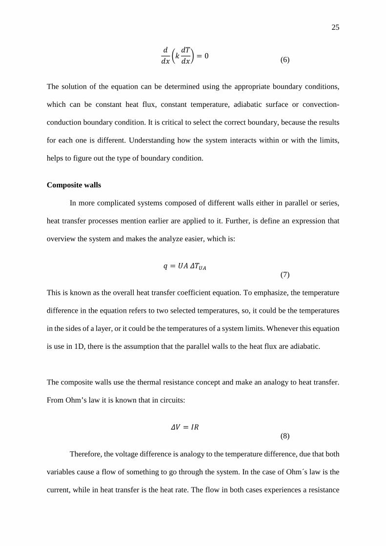
This equation is known as the heat diffusion equation. Several assumptions can be done, to
define an adequate expression for the system to analyzed. Under steady state condition, 1D
dimension, it can be found that the equation reduces to.
25
𝑑𝑑𝑑𝑑𝑑𝑑
�𝑘𝑘𝑑𝑑𝑇𝑇𝑑𝑑𝑑𝑑� = 0
(6)
The solution of the equation can be determined using the appropriate boundary conditions,
which can be constant heat flux, constant temperature, adiabatic surface or convection-
conduction boundary condition. It is critical to select the correct boundary, because the results
for each one is different. Understanding how the system interacts within or with the limits,
helps to figure out the type of boundary condition.
Composite walls
In more complicated systems composed of different walls either in parallel or series,
heat transfer processes mention earlier are applied to it. Further, is define an expression that
overview the system and makes the analyze easier, which is:
𝑞𝑞 = 𝑈𝑈𝐴𝐴 𝛥𝛥𝑇𝑇𝑈𝑈𝑈𝑈
(7) This is known as the overall heat transfer coefficient equation. To emphasize, the temperature
difference in the equation refers to two selected temperatures, so, it could be the temperatures
in the sides of a layer, or it could be the temperatures of a system limits. Whenever this equation
is use in 1D, there is the assumption that the parallel walls to the heat flux are adiabatic.
The composite walls use the thermal resistance concept and make an analogy to heat transfer.
From Ohm’s law it is known that in circuits:
𝛥𝛥𝛥𝛥 = 𝐼𝐼𝑅𝑅
(8)
Therefore, the voltage difference is analogy to the temperature difference, due that both
variables cause a flow of something to go through the system. In the case of Ohm´s law is the
current, while in heat transfer is the heat rate. The flow in both cases experiences a resistance
26
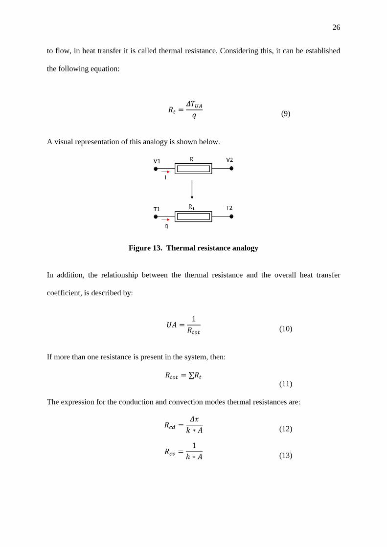
to flow, in heat transfer it is called thermal resistance. Considering this, it can be established
the following equation:
𝑅𝑅𝑜𝑜 =𝛥𝛥𝑇𝑇𝑈𝑈𝑈𝑈𝑞𝑞
(9)
A visual representation of this analogy is shown below.
Figure 13. Thermal resistance analogy
In addition, the relationship between the thermal resistance and the overall heat transfer
coefficient, is described by:
𝑈𝑈𝐴𝐴 =1𝑅𝑅𝑜𝑜𝑜𝑜𝑜𝑜
(10)
If more than one resistance is present in the system, then:
𝑅𝑅𝑜𝑜𝑜𝑜𝑜𝑜 = ∑𝑅𝑅𝑜𝑜
(11)
The expression for the conduction and convection modes thermal resistances are:
𝑅𝑅𝑐𝑐𝑐𝑐 =𝛥𝛥𝑑𝑑𝑘𝑘 ∗ 𝐴𝐴
(12)
𝑅𝑅𝑐𝑐𝑐𝑐 =1
ℎ ∗ 𝐴𝐴
(13)
27
2.1.2 Fundamentals of fluid mechanics.
This physics overview the development, forces, conditions that the fluid experiences in
a continuum movement. To analyzed properly a fluid, the flow condition and the fluid type
must be determined first. There are two types of fluids: laminar or turbulent, which depends
on the fluid velocity. A laminar fluid characterizes to be smooth with streamlines parallel to
each other. On the other hand, a turbulent flow is a chaotic fluid which drown to vortices inside
the fluid, to mix it. The velocity in the second type is higher than the first type. Also, there is a
transition zone from the laminar to the turbulent flow; in this zone the fluid shares a mix of
both flow types features.
Flow conditions
To determine the type of flow a dimensionless number know as Reynolds. It helps to
identify the type of flow by a numerical range, which separate the laminar from the turbulent
region. Also, it depends where the fluid goes through, outside or inside the system. For
example, the cooling of a chip using a blowing fan is an external flow and a heating ventilation
system using cooper lines is an internal flow. The Re definition is:
𝑅𝑅𝑅𝑅 =𝜌𝜌𝑢𝑢𝐷𝐷
µ
(14)
However, in a pipe fluid analysis the Re can be computed using the mass flow rate1.
𝑅𝑅𝑅𝑅𝐷𝐷 =4�̇�𝑚𝜋𝜋𝐷𝐷µ
(15)
In such cases, a transition number know as critical Re (𝑅𝑅𝑅𝑅𝑐𝑐𝑐𝑐) is established.
1 It is a more common used variable in situations with pipes
28
Losses by friction in pipes
Furthermore, the fluid experiences forces on it when it goes through a pipe. Such forces
like: body and contact. Body forces correspond to the gravity. A contact force is the friction
force that creates between the walls and the fluid. It depends on the rugosity of the material of
the pipe, identify it by smooth or a rough pipe. Also, the friction force has influence on the
velocity of the pipe, due that it causes changes in the direction of the fluid at the solid-fluid
interface. The equation that describes the effect of friction is the Darcy-Weisbach equation,
which is:
ℎ𝑓𝑓 =𝑓𝑓𝐿𝐿𝑣𝑣2
𝐷𝐷2𝑔𝑔
(16)
The friction factor (f) is obtained from the Colebrook equation2, that is applied either for any
range of Reynolds number.
1�𝑓𝑓
= −2 𝑙𝑙𝑙𝑙𝑔𝑔 𝑙𝑙𝑙𝑙𝑔𝑔 (𝜀𝜀𝐼𝐼𝐷𝐷3.7
+2.51
(𝑅𝑅𝑅𝑅)𝑓𝑓0.5
(17)
The velocity change also affects the pressure in the system when its experience forces, because
they are directly proportional by the Bernoulli equation.
𝑣𝑣12
2𝑔𝑔+𝑝𝑝1𝜌𝜌𝑔𝑔
+ 𝑑𝑑1 =𝑣𝑣22
2𝑔𝑔+𝑝𝑝2𝜌𝜌𝑔𝑔
+ 𝑑𝑑2 + ℎ𝑙𝑙
(18)
Where: ℎ𝑙𝑙 accounts for major losses (ℎ𝑓𝑓) and minor losses (ℎ𝑚𝑚) in the pipe. Major losses are associate
with the friction effects and minor losses to bends, fittings, contractions, expansion, etc. Thus:
ℎ𝑙𝑙 = ℎ𝑓𝑓 + ℎ𝑚𝑚
(19)
2 This equation is use instead of the Moody chart

29
Minor losses are determine with the following expression:
ℎ𝑚𝑚 =𝑘𝑘𝑣𝑣2
𝐷𝐷2𝑔𝑔
(20)
Fluids momentum conservation
Moreover, an essential part of fluid mechanics is the conservation of momentum. This
overview how the fluid interacts with the solid interface. The layout of the pipe is an essential
factor to consider when is analyzed. Especially when the pipe has bends, contractions or
expansions. Bends causes the fluid to change direction and its momentum. The Navier-Stokes
equation describes the change in momentum a fluid experiences in a fluid domain with its
boundaries, which is:
∑𝐹𝐹 =𝑑𝑑𝑑𝑑𝑑𝑑∫𝑐𝑐𝑐𝑐𝜌𝜌𝑣𝑣𝑑𝑑𝑣𝑣 + ∑𝑐𝑐𝑠𝑠𝜌𝜌𝑣𝑣(𝑣𝑣 ∗ 𝐴𝐴)
(21)
2.1.3 Conjugate Heat Transfer: Internal Flow.
For more complicated problems that deal with the coupling of heat transfer and fluid
mechanics, the conjugate heat transfer physics is use and if is inside a pipe, is name internal
flow.
Boundary layers
Due to the solid-fluid interaction, a boundary layer developed for both velocity and
temperature variables. The boundary layer describes the graphical behavior of the profile of
the variable in study, as follows. As a fluid is confined and a volumetric flow rate is set to it:
30
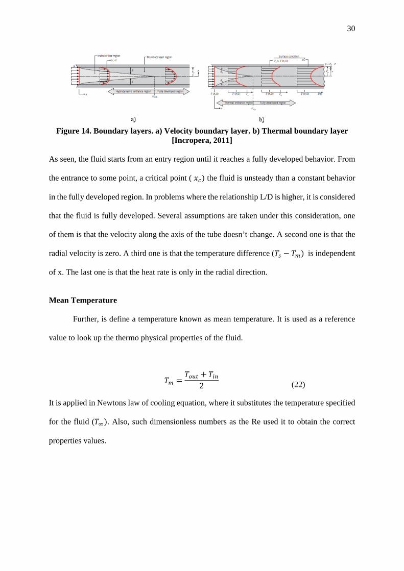
Figure 14. Boundary layers. a) Velocity boundary layer. b) Thermal boundary layer
[Incropera, 2011] As seen, the fluid starts from an entry region until it reaches a fully developed behavior. From
the entrance to some point, a critical point ( 𝑑𝑑𝑐𝑐) the fluid is unsteady than a constant behavior
in the fully developed region. In problems where the relationship L/D is higher, it is considered
that the fluid is fully developed. Several assumptions are taken under this consideration, one
of them is that the velocity along the axis of the tube doesn’t change. A second one is that the
radial velocity is zero. A third one is that the temperature difference (𝑇𝑇𝑠𝑠 − 𝑇𝑇𝑚𝑚) is independent
of x. The last one is that the heat rate is only in the radial direction.
Mean Temperature
Further, is define a temperature known as mean temperature. It is used as a reference
value to look up the thermo physical properties of the fluid.
𝑇𝑇𝑚𝑚 =𝑇𝑇𝑜𝑜𝑜𝑜𝑜𝑜 + 𝑇𝑇𝑖𝑖𝑖𝑖
2
(22)
It is applied in Newtons law of cooling equation, where it substitutes the temperature specified
for the fluid (𝑇𝑇∞). Also, such dimensionless numbers as the Re used it to obtain the correct
properties values.
31
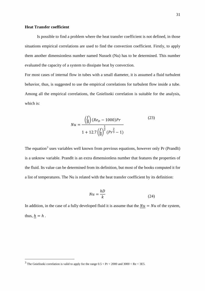
Heat Transfer coefficient
Is possible to find a problem where the heat transfer coefficient is not defined, in those
situations empirical correlations are used to find the convection coefficient. Firstly, to apply
them another dimensionless number named Nusselt (Nu) has to be determined. This number
evaluated the capacity of a system to dissipate heat by convection.
For most cases of internal flow in tubes with a small diameter, it is assumed a fluid turbulent
behavior, thus, is suggested to use the empirical correlations for turbulent flow inside a tube.
Among all the empirical correlations, the Gnielisnki correlation is suitable for the analysis,
which is:
𝑁𝑁𝑢𝑢 =�𝑓𝑓8� (𝑅𝑅𝑅𝑅𝐷𝐷 − 1000)𝑃𝑃𝑃𝑃
1 + 12.7 �𝑓𝑓8�12
(𝑃𝑃𝑃𝑃23 − 1)
(23)
The equation3 uses variables well known from previous equations, however only Pr (Prandlt)
is a unknow variable. Prandlt is an extra dimensionless number that features the properties of
the fluid. Its value can be determined from its definition, but most of the books computed it for
a list of temperatures. The Nu is related with the heat transfer coefficient by its definition:
𝑁𝑁𝑢𝑢 =ℎ𝐷𝐷𝑘𝑘
(24)
In addition, in the case of a fully developed fluid it is assume that the 𝑁𝑁𝑢𝑢 = 𝑁𝑁𝑢𝑢 of the system,
thus, ℎ = ℎ .
3 The Gnielisnki correlation is valid to apply for the range 0.5 < Pr < 2000 and 3000 < Re < 3E5.

32
Internal energy
In a heat transfer exchange between a solid and fluid, it can occur a change in the
temperature of the fluid, meaning its internal energy increases. Regarding an incompressible
fluid and a conservation of energy analysis, the following expression is defined.
𝑞𝑞 = �̇�𝑚𝐶𝐶𝑝𝑝𝛥𝛥𝑇𝑇𝐼𝐼𝐼𝐼 = �̇�𝑚𝐶𝐶𝑝𝑝(𝑇𝑇𝑜𝑜𝑜𝑜𝑜𝑜 − 𝑇𝑇𝑖𝑖𝑖𝑖)
(25) The equation known as thermal energy comes out under a sensible heat simplification and
assumptions such as: no latent heat changes, no generation, negligible potential and kinetic
energy, steady flow.
Figure 15. Thermal energy ilustration4
2.1.4 Fundamentals applied to the system.
Once review the fundamentals of fluid mechanics and heat transfer, they are applied to
the problem of study. Then, it must be understood what is known from it to proceed to the
correct analysis.
System overview
It is known: the geometry properties, that include the diameters of the tube to use and
the dimensions of the RBx and its modules; the materials of the system, which are water for
the fluid and Aluminum 6061 for the solid parts; the heat load specified by module from the
RBx; the volumetric flow rate (Q) and the inlet temperature of the fluid. This information is
4 The temperatures are taken as average temperatures computed over the cross section specified.
33
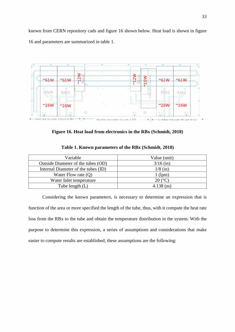
known from CERN repository cads and figure 16 shown below. Heat load is shown in figure
16 and parameters are summarized in table 1.
Figure 16. Heat load from electronics in the RBx (Schmidt, 2018)
Table 1. Known parameters of the RBx (Schmidt, 2018)
Variable Value (unit) Outside Diameter of the tubes (OD) 3/16 (in) Internal Diameter of the tubes (ID) 1/8 (in)
Water Flow rate (Q) 1 (lpm) Water Inlet temperature 20 (°C)
Tube length (L) 4.138 (m)
Considering the known parameters, is necessary to determine an expression that is
function of the area or more specified the length of the tube, thus, with it compute the heat rate
loss from the RBx to the tube and obtain the temperature distribution in the system. With the
purpose to determine this expression, a series of assumptions and considerations that make
easier to compute results are established, these assumptions are the following:
34
Table 2. Heat transfer analysis assumptions
One dimensional analysis Cooper resistance is negligible
Steady state system No fouling consider Fully developed flow No corrosion consider
Incompressible fluid without phase changes Cooper resistance is negligible No conduction in the fluid, just convection No radiation consider
Isotropic materials No contact resistances consider Bousiness approximation taken for the fluid5
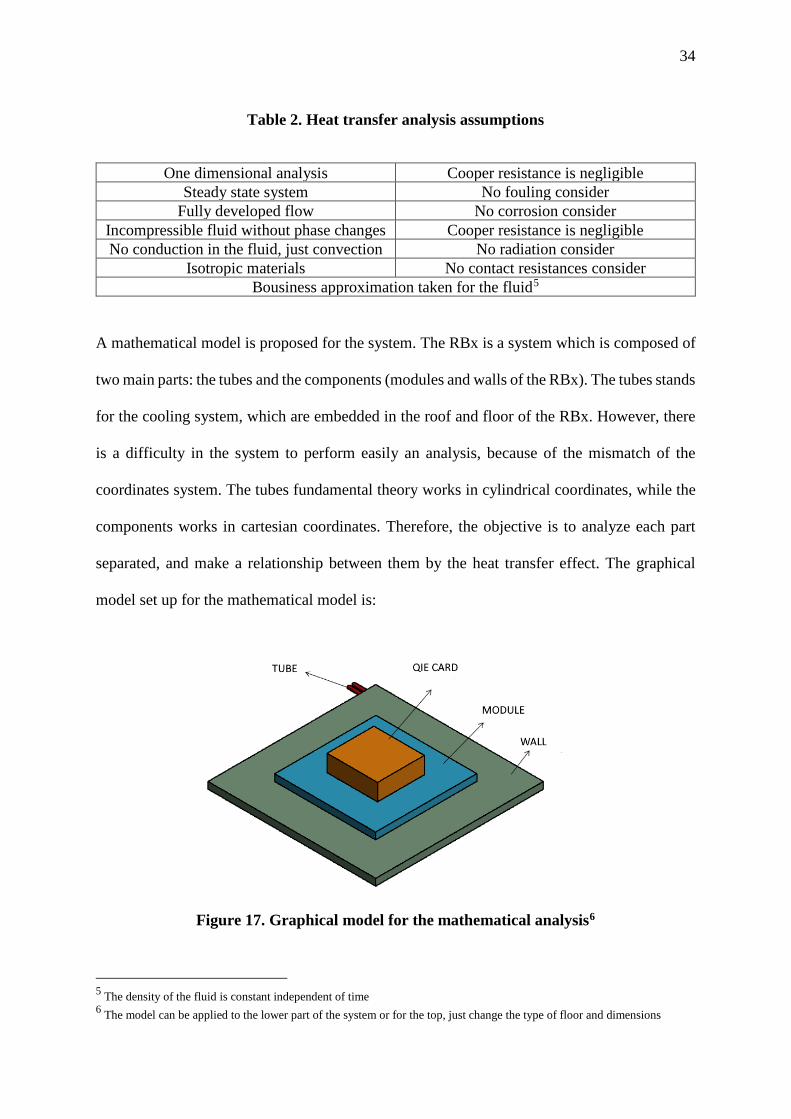
A mathematical model is proposed for the system. The RBx is a system which is composed of
two main parts: the tubes and the components (modules and walls of the RBx). The tubes stands
for the cooling system, which are embedded in the roof and floor of the RBx. However, there
is a difficulty in the system to perform easily an analysis, because of the mismatch of the
coordinates system. The tubes fundamental theory works in cylindrical coordinates, while the
components works in cartesian coordinates. Therefore, the objective is to analyze each part
separated, and make a relationship between them by the heat transfer effect. The graphical
model set up for the mathematical model is:
Figure 17. Graphical model for the mathematical analysis6
5 The density of the fluid is constant independent of time 6 The model can be applied to the lower part of the system or for the top, just change the type of floor and dimensions
35
Where:
QIE card: stands for the whole bunch of QIE cards in the modules.
Module: stands for the total wall thickness of the modules in the RBx (CM, CCM, RM).
Wall: stands for the external wall thickness of the RBx.
Tube: stands for the tube that belongs to the selected wall.
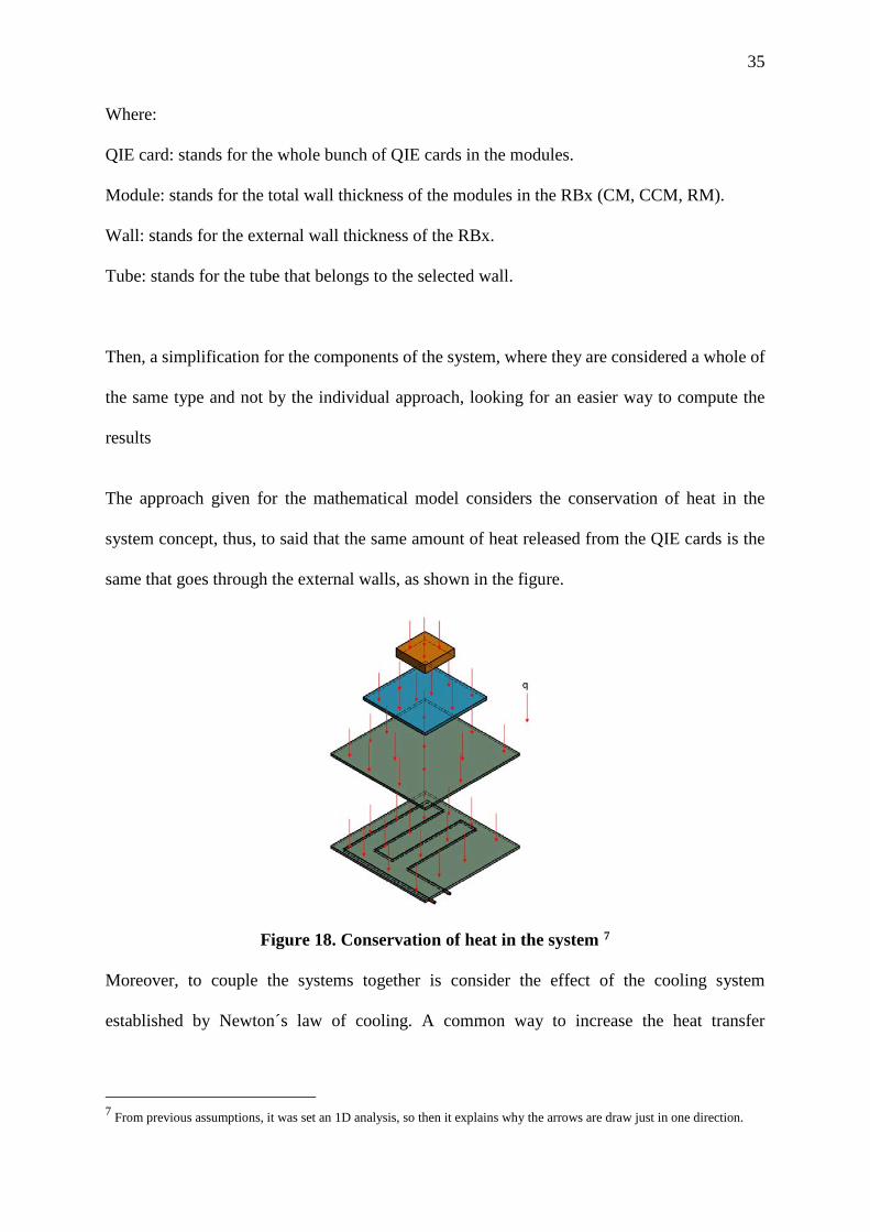
Then, a simplification for the components of the system, where they are considered a whole of
the same type and not by the individual approach, looking for an easier way to compute the
results
The approach given for the mathematical model considers the conservation of heat in the
system concept, thus, to said that the same amount of heat released from the QIE cards is the
same that goes through the external walls, as shown in the figure.
Figure 18. Conservation of heat in the system 7 Moreover, to couple the systems together is consider the effect of the cooling system
established by Newton´s law of cooling. A common way to increase the heat transfer
7 From previous assumptions, it was set an 1D analysis, so then it explains why the arrows are draw just in one direction.
36
convection is by increasing the h, however, is expensive. Therefore, the suitable option is to
increase the tube length and then the area of the tube occupied
inally, using equation a n expression of tempe rature as function of lengt h of the tube is obtaine d.
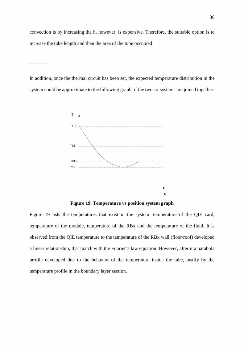
In addition, once the thermal circuit has been set, the expected temperature distribution in the
system could be approximate to the following graph, if the two co-systems are joined together.
Figure 19. Temperature vs position system graph
Figure 19 lists the temperatures that exist in the system: temperature of the QIE card,
temperature of the module, temperature of the RBx and the temperature of the fluid. It is
observed from the QIE temperature to the temperature of the RBx wall (floor/roof) developed
a linear relationship, that match with the Fourier’s law equation. However, after it a parabola
profile developed due to the behavior of the temperature inside the tube, justify by the
temperature profile in the boundary layer section.
37
Under this graphical model and mathematical model, it has been proposed a guide with a series
of steps in order to obtain an expression which relates the length of the tube and temperature.
As detail below:
1.- Determine the 𝑇𝑇𝑜𝑜𝑜𝑜𝑜𝑜 of the fluid by using: q = �̇�𝑚𝐶𝐶𝑝𝑝𝛥𝛥𝑇𝑇
2.- Obtain 𝑇𝑇𝑚𝑚 and use it to compute the fluid properties
3.- Determine the �̇�𝑚 by using the continuity equation and then compute the Re by using
equation 15. Once the Re is obtained, the friction factor can be determined from the Colebrook
equation. Using the results of the f and Re, the Nu can be computed from the Gnielisnki
correlation. Then, h is obtained from the Nu definition.
4.- Set the thermal circuit for the system and determine the resistances and its expressions by
using equations 12 & 13. Further, compute the total resistance by using equation 11 in terms
of the length of the tube.
5. – Using equation 10 the UA can be obtained, and at last using equation 7 the function of the
temperature difference in terms of the length can be obtained.
38
2.2 CFD Analysis
2.2.1 Comsol Multiphysics Overview.
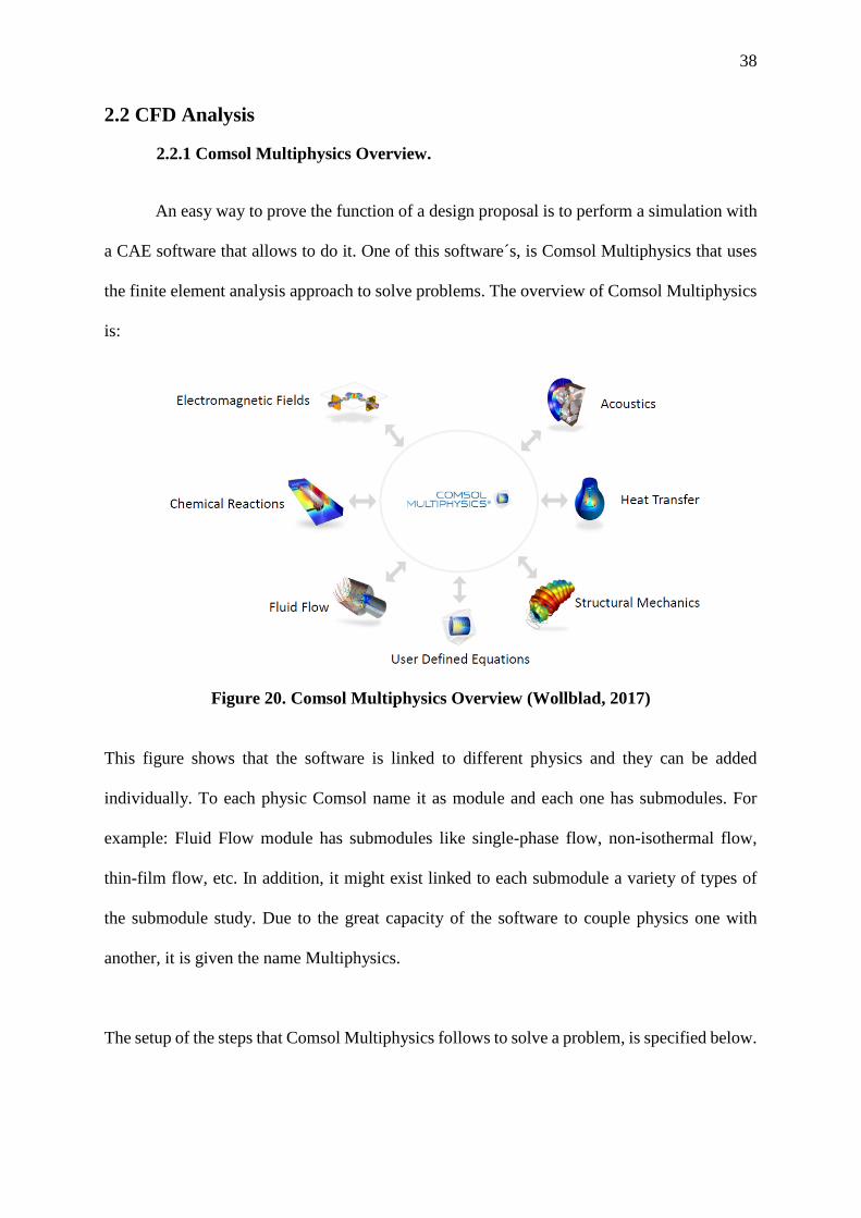
An easy way to prove the function of a design proposal is to perform a simulation with
a CAE software that allows to do it. One of this software´s, is Comsol Multiphysics that uses
the finite element analysis approach to solve problems. The overview of Comsol Multiphysics
is:
Figure 20. Comsol Multiphysics Overview (Wollblad, 2017)
This figure shows that the software is linked to different physics and they can be added
individually. To each physic Comsol name it as module and each one has submodules. For
example: Fluid Flow module has submodules like single-phase flow, non-isothermal flow,
thin-film flow, etc. In addition, it might exist linked to each submodule a variety of types of
the submodule study. Due to the great capacity of the software to couple physics one with
another, it is given the name Multiphysics.
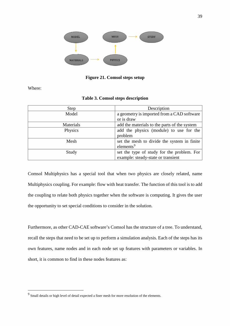
The setup of the steps that Comsol Multiphysics follows to solve a problem, is specified below.
39
Figure 21. Comsol steps setup
Where:
Table 3. Comsol steps description
Step Description Model a geometry is imported from a CAD software
or is draw Materials add the materials to the parts of the system Physics add the physics (module) to use for the
problem Mesh set the mesh to divide the system in finite
elements9 Study set the type of study for the problem. For
example: steady-state or transient Comsol Multiphysics has a special tool that when two physics are closely related, name
Multiphysics coupling. For example: flow with heat transfer. The function of this tool is to add
the coupling to relate both physics together when the software is computing. It gives the user
the opportunity to set special conditions to consider in the solution.
Furthermore, as other CAD-CAE software’s Comsol has the structure of a tree. To understand,
recall the steps that need to be set up to perform a simulation analysis. Each of the steps has its
own features, name nodes and in each node set up features with parameters or variables. In
short, it is common to find in these nodes features as:
9 Small details or high level of detail expected a finer mesh for more resolution of the elements.
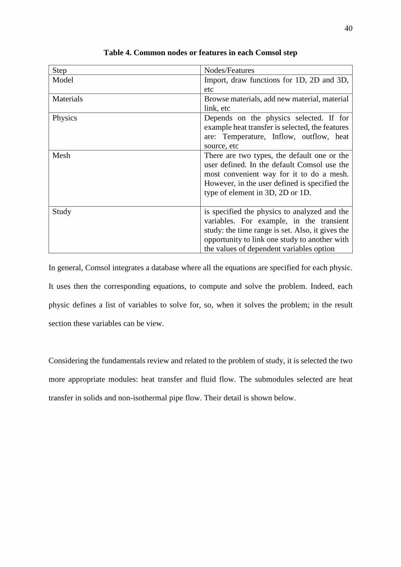
40
Table 4. Common nodes or features in each Comsol step
Step Nodes/Features Model Import, draw functions for 1D, 2D and 3D,
etc Materials Browse materials, add new material, material
link, etc Physics Depends on the physics selected. If for
example heat transfer is selected, the features are: Temperature, Inflow, outflow, heat source, etc
Mesh There are two types, the default one or the user defined. In the default Comsol use the most convenient way for it to do a mesh. However, in the user defined is specified the type of element in 3D, 2D or 1D.
Study is specified the physics to analyzed and the variables. For example, in the transient study: the time range is set. Also, it gives the opportunity to link one study to another with the values of dependent variables option
In general, Comsol integrates a database where all the equations are specified for each physic.
It uses then the corresponding equations, to compute and solve the problem. Indeed, each
physic defines a list of variables to solve for, so, when it solves the problem; in the result
section these variables can be view.
Considering the fundamentals review and related to the problem of study, it is selected the two
more appropriate modules: heat transfer and fluid flow. The submodules selected are heat
transfer in solids and non-isothermal pipe flow. Their detail is shown below.

41
2.2.1.1 Heat transfer in Solids module.
This module analyzes heat transfer modes, such as: conduction, convection and
radiation in a solid. However, it can specify a fluid domain in the system and this field is
recognize for the software as fluid. The variable solved in the module is the temperature. The
most common nodes or conditions that are set up in this module are:
Table 5. Common nodes or features for heat transfer in solids module
Node/Feature Description Temperature B.C to set a boundary with a specified
temperature Heat flux Set a boundary with the ability to generate or
exchange heat. It can be set a general inward heat flux condition, a convective heat flux condition and a heat rate condition
Thermal insulation By default, those boundaries that are not specified by a condition, are set up in this condition. It defines an adiabatic wall condition, meaning that there is not heat transfer interface due that it lacks a temperature difference
Heat source Set a boundary or a domain a heat generated Initial values Set the initial values for a transient analysis
regarding the variable solve for in the module.
Solid Associate the domain selected to a material The equation that is used in the heat transfer in solids module is the following:
𝜌𝜌𝐶𝐶𝑝𝑝𝑑𝑑𝑇𝑇𝑑𝑑𝑑𝑑
− 𝛻𝛻(𝑘𝑘𝛻𝛻𝑇𝑇) = 𝑄𝑄
(29)
As noticed the equation comes from the first law of thermodynamics. Is like the heat diffusion
equation but displayed in a different way. The first term accounts for the energy change in
time; the second accounts for the conduction term; and at last the term in the right accounts for
the heat generation in the system. For steady-state problems, the first term is zero (COMSOL,
2014).
42
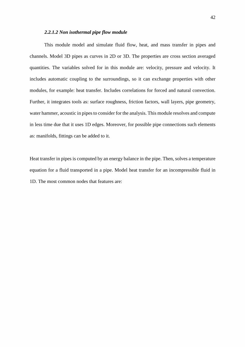
2.2.1.2 Non isothermal pipe flow module
This module model and simulate fluid flow, heat, and mass transfer in pipes and
channels. Model 3D pipes as curves in 2D or 3D. The properties are cross section averaged
quantities. The variables solved for in this module are: velocity, pressure and velocity. It
includes automatic coupling to the surroundings, so it can exchange properties with other
modules, for example: heat transfer. Includes correlations for forced and natural convection.
Further, it integrates tools as: surface roughness, friction factors, wall layers, pipe geometry,
water hammer, acoustic in pipes to consider for the analysis. This module resolves and compute
in less time due that it uses 1D edges. Moreover, for possible pipe connections such elements
as: manifolds, fittings can be added to it.
Heat transfer in pipes is computed by an energy balance in the pipe. Then, solves a temperature
equation for a fluid transported in a pipe. Model heat transfer for an incompressible fluid in
1D. The most common nodes that features are:
43
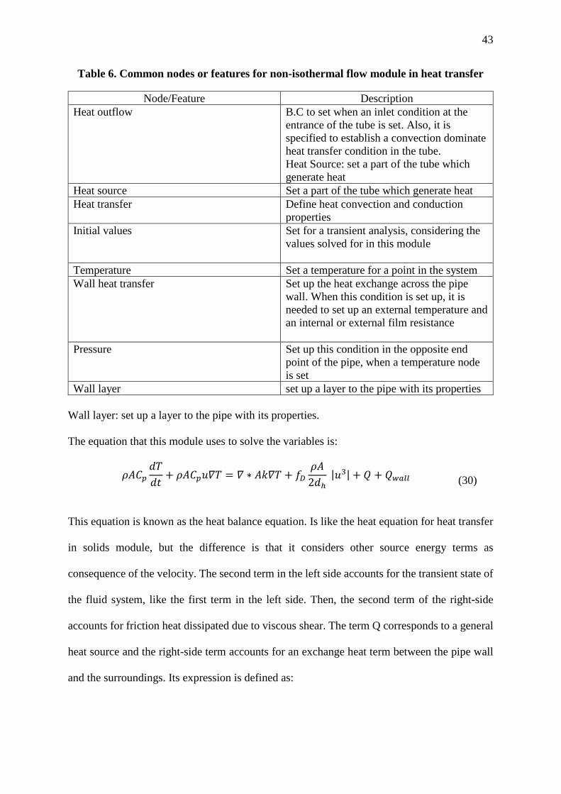
Table 6. Common nodes or features for non-isothermal flow module in heat transfer
Node/Feature Description Heat outflow B.C to set when an inlet condition at the
entrance of the tube is set. Also, it is specified to establish a convection dominate heat transfer condition in the tube. Heat Source: set a part of the tube which generate heat
Heat source Set a part of the tube which generate heat Heat transfer Define heat convection and conduction
properties Initial values Set for a transient analysis, considering the
values solved for in this module
Temperature Set a temperature for a point in the system Wall heat transfer Set up the heat exchange across the pipe
wall. When this condition is set up, it is needed to set up an external temperature and an internal or external film resistance
Pressure Set up this condition in the opposite end point of the pipe, when a temperature node is set
Wall layer set up a layer to the pipe with its properties Wall layer: set up a layer to the pipe with its properties. The equation that this module uses to solve the variables is:
𝜌𝜌𝐴𝐴𝐶𝐶𝑝𝑝𝑑𝑑𝑇𝑇𝑑𝑑𝑑𝑑
+ 𝜌𝜌𝐴𝐴𝐶𝐶𝑝𝑝𝑢𝑢𝛻𝛻𝑇𝑇 = 𝛻𝛻 ∗ 𝐴𝐴𝑘𝑘𝛻𝛻𝑇𝑇 + 𝑓𝑓𝐷𝐷𝜌𝜌𝐴𝐴2𝑑𝑑ℎ
|𝑢𝑢3| + 𝑄𝑄 + 𝑄𝑄𝑤𝑤𝑤𝑤𝑙𝑙𝑙𝑙
(30)
This equation is known as the heat balance equation. Is like the heat equation for heat transfer
in solids module, but the difference is that it considers other source energy terms as
consequence of the velocity. The second term in the left side accounts for the transient state of
the fluid system, like the first term in the left side. Then, the second term of the right-side
accounts for friction heat dissipated due to viscous shear. The term Q corresponds to a general
heat source and the right-side term accounts for an exchange heat term between the pipe wall
and the surroundings. Its expression is defined as:
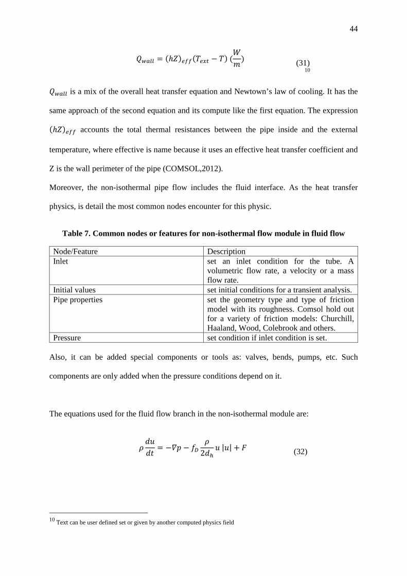
44
𝑄𝑄𝑤𝑤𝑤𝑤𝑙𝑙𝑙𝑙 = (ℎ𝑍𝑍)𝑔𝑔𝑓𝑓𝑓𝑓(𝑇𝑇𝑔𝑔𝑥𝑥𝑜𝑜 − 𝑇𝑇) (𝑊𝑊𝑚𝑚
)
(31)
10 𝑄𝑄𝑤𝑤𝑤𝑤𝑙𝑙𝑙𝑙 is a mix of the overall heat transfer equation and Newtown’s law of cooling. It has the
same approach of the second equation and its compute like the first equation. The expression
(ℎ𝑍𝑍)𝑔𝑔𝑓𝑓𝑓𝑓 accounts the total thermal resistances between the pipe inside and the external
temperature, where effective is name because it uses an effective heat transfer coefficient and
Z is the wall perimeter of the pipe (COMSOL,2012).
Moreover, the non-isothermal pipe flow includes the fluid interface. As the heat transfer
physics, is detail the most common nodes encounter for this physic.
Table 7. Common nodes or features for non-isothermal flow module in fluid flow
Node/Feature Description Inlet set an inlet condition for the tube. A
volumetric flow rate, a velocity or a mass flow rate.
Initial values set initial conditions for a transient analysis. Pipe properties set the geometry type and type of friction
model with its roughness. Comsol hold out for a variety of friction models: Churchill, Haaland, Wood, Colebrook and others.
Pressure set condition if inlet condition is set. Also, it can be added special components or tools as: valves, bends, pumps, etc. Such
components are only added when the pressure conditions depend on it.
The equations used for the fluid flow branch in the non-isothermal module are:
𝜌𝜌𝑑𝑑𝑢𝑢𝑑𝑑𝑑𝑑
= −𝛻𝛻𝑝𝑝 − 𝑓𝑓𝐷𝐷𝜌𝜌
2𝑑𝑑ℎ𝑢𝑢 |𝑢𝑢| + 𝐹𝐹
(32)
10 Text can be user defined set or given by another computed physics field
45
This equation is the momentum equation and is like the Navier-Stockes equation set before,
with an additional term and displayed in a different way. Some terms are common from both
equations, however, the second term in the right-side accounts for the pressure drop due to the
viscous shear. The F expression is a volume force term.
And the second equation is:
𝑑𝑑𝐴𝐴𝜌𝜌𝑑𝑑𝑑𝑑
+ 𝛻𝛻 ∗ (𝐴𝐴𝜌𝜌𝑢𝑢) = 0
(33)
Which is the continuity equation.
2.2.2 System design and analysis
Since there are some limitations in the modeling due to the mesh, it is selected an
approximated model to the real one that represents mostly the system. The details neglected
for this model are: holes, filets and chamfers. Also, elements irrelevant to the physics analyzed
as: wire, extra modules. However, firstly what is consider is the tube design in the floor wall,
because the system depends on it.
2.2.2.1 Overview of tube design
In general, a cooling system main task is to exchange heat from a source to a destination.
Thus, the system lowers its temperature from its initial condition. It can change in its design
and application, but it always searches to accomplish to reduce the temperature. The selected
one in this case is by using cooper tubes as media to reduce the temperature of the QIE cards.
Applications examples such as: ceiling floors, geothermal heating loops, oil pipelines
insulation, cold plates, heat pipes for desktop show the versatility of the topic.
46
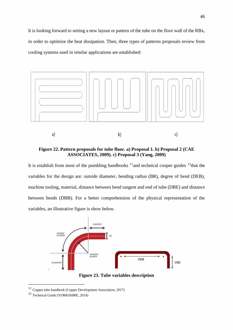
It is looking forward to setting a new layout or pattern of the tube on the floor wall of the RBx,
in order to optimize the heat dissipation. Then, three types of patterns proposals review from
cooling systems used in similar applications are established:
Figure 22. Pattern proposals for tube floor. a) Proposal 1. b) Proposal 2 (CAE ASSOCIATES, 2009). c) Proposal 3 (Yang, 2009)
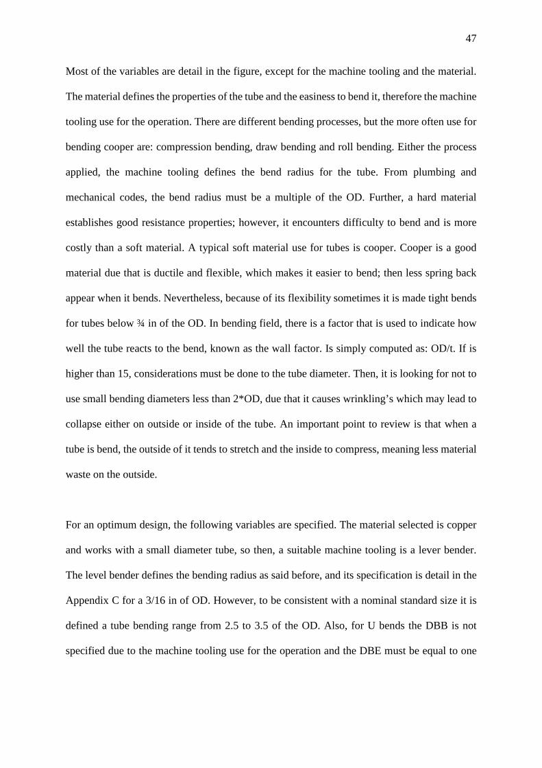
It is establish from most of the pumbling handbooks 11and technical cooper guides 12that the
variables for the design are: outside diameter, bending radius (BR), degree of bend (DEB),
machine tooling, material, distance between bend tangent and end of tube (DBE) and distance
between bends (DBB). For a better comprehension of the physical representation of the
variables, an illustrative figure is show below.
Figure 23. Tube variables description
11 Copper tube handbook (Copper Development Association, 2017) 12 Technical Guide (YORKSHIRE, 2014)
47
Most of the variables are detail in the figure, except for the machine tooling and the material.
The material defines the properties of the tube and the easiness to bend it, therefore the machine
tooling use for the operation. There are different bending processes, but the more often use for
bending cooper are: compression bending, draw bending and roll bending. Either the process
applied, the machine tooling defines the bend radius for the tube. From plumbing and
mechanical codes, the bend radius must be a multiple of the OD. Further, a hard material
establishes good resistance properties; however, it encounters difficulty to bend and is more
costly than a soft material. A typical soft material use for tubes is cooper. Cooper is a good
material due that is ductile and flexible, which makes it easier to bend; then less spring back
appear when it bends. Nevertheless, because of its flexibility sometimes it is made tight bends
for tubes below ¾ in of the OD. In bending field, there is a factor that is used to indicate how
well the tube reacts to the bend, known as the wall factor. Is simply computed as: OD/t. If is
higher than 15, considerations must be done to the tube diameter. Then, it is looking for not to
use small bending diameters less than 2*OD, due that it causes wrinkling’s which may lead to
collapse either on outside or inside of the tube. An important point to review is that when a
tube is bend, the outside of it tends to stretch and the inside to compress, meaning less material
waste on the outside.
For an optimum design, the following variables are specified. The material selected is copper
and works with a small diameter tube, so then, a suitable machine tooling is a lever bender.
The level bender defines the bending radius as said before, and its specification is detail in the
Appendix C for a 3/16 in of OD. However, to be consistent with a nominal standard size it is
defined a tube bending range from 2.5 to 3.5 of the OD. Also, for U bends the DBB is not
specified due to the machine tooling use for the operation and the DBE must be equal to one
48
OD. In the case of the layout design, the degree of bend for all the bends is 90 degrees. Possible
modifications be done if the wall factor goes beyond the limits
A methodology is implemented to obtain the optimum tube layout. It considers the space to
occupy and the design variables. For the first pattern proposal is detail explicitly, but for the
rest of proposals just the design layout is shown.
Design
In the design, it is wanted to increase the number of loops, so the length tube increases
as well. The methodology is to setup parameters for the segments of the layout, then establish
a program that uses the variables to compute and find out the optimum design. The optimum
design must fulfil all the design variables and is the longest one.
It has been established three types of variables: general, fill and modified. The general features
are measurements obtained from CERN repository cads and they are preserved for all the
designs. The modified variables are those that are used to modify the number of loops (n). And
finally the fill variables are used to fill measures of the layout. In each proposal the modified
and fill variables are different, due that each layout is unique. In addition, in order to obtain the
real length of the tube layout, extra variables are defined. Its only function is to help
determining the total length (𝐿𝐿𝑇𝑇) of the tube.
The specification of the three types of variables is listed below.

49
Table 8. Specification and values for the general variables of the design proposals
General variables Specification Value (m)
H accounts for the max height of the design space for the layout
0.304
W accounts for the max width of the design space for the layout
0.965
W separation between the starting point and the end point of the layout
0.018
O separation between the limit and the starting point of the layout
0.0127
H Tube length fill end h = OD
0.0047625
A separation between the layout and the limits
It is established that a = O
0.0127
C separation between the layout and the back-side end. Is the sum of parameter b and a. The parameter b accounts for a geometry interference.
b = 0.0144
c = b+a
Table 9. Detail of the fill and modified variables of the design proposals
Design proposal Type of variable Fill Modified Extra
1 L1, L2 L3, L4 C113 2 L1, L4, L5 L2, L3 3 L1, L5, L6 L2, L3, L4
Due to the complexity of not knowing the tube bending optimum diameter exactly. It is
established a user-friendly program by Octave Online Editor, which use the variables of the
figure and just vary the number of loops with the modified parameters. This optimum bending
13 defines a single pipe bend (curve), not all the U shape
50
diameter is looking forward for not to be the min or max limits of the bending diameter degree,
due that a less diameter involves higher effects of corrosion and dirtiness, and a larger diameter
is not ideal for optimize the use of available space. Therefore, this diameter in addition has to
be one which satisfies a long length, not too long or short, besides the conditions that has to
fulfil. Then, it is correct to select the bending radius that the machine tooling specified. The
purpose is then to obtain maximum number of loops for it. The scripts can be check out in
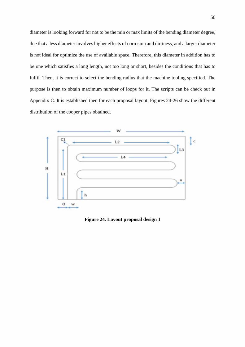
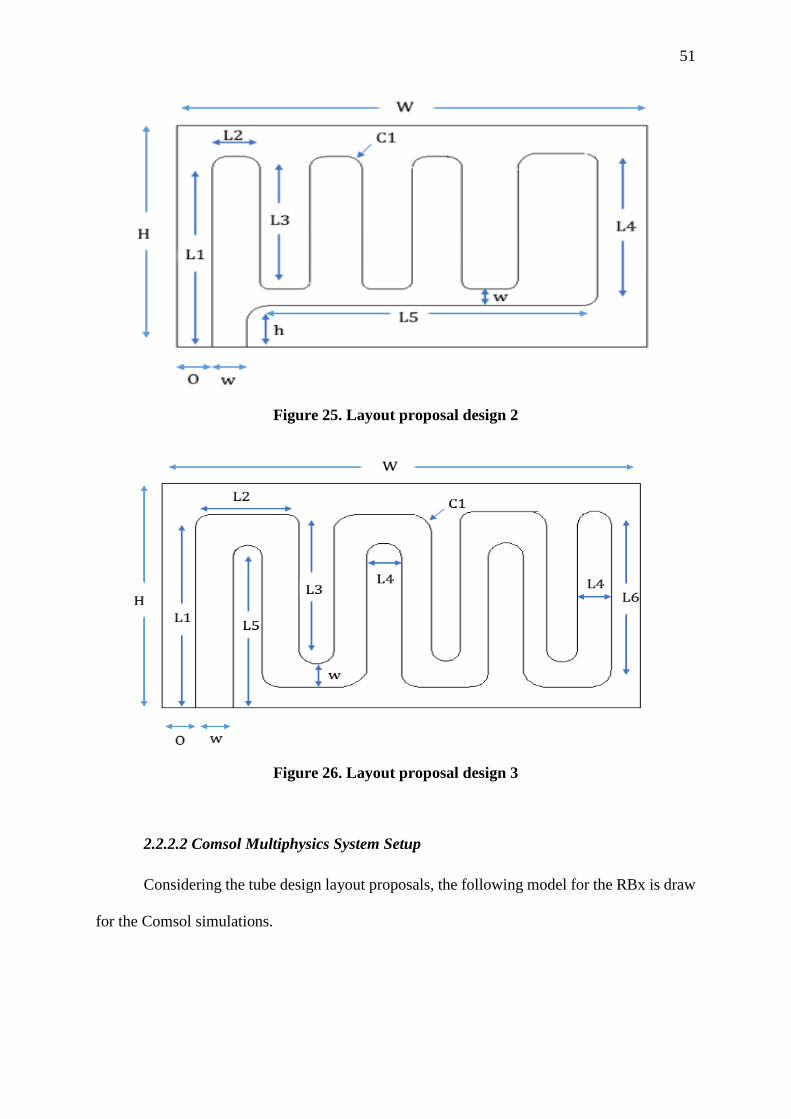
Appendix C. It is established then for each proposal layout. Figures 24-26 show the different
distribution of the cooper pipes obtained.
Figure 24. Layout proposal design 1
51
Figure 25. Layout proposal design 2
Figure 26. Layout proposal design 3
2.2.2.2 Comsol Multiphysics System Setup
Considering the tube design layout proposals, the following model for the RBx is draw
for the Comsol simulations.
52
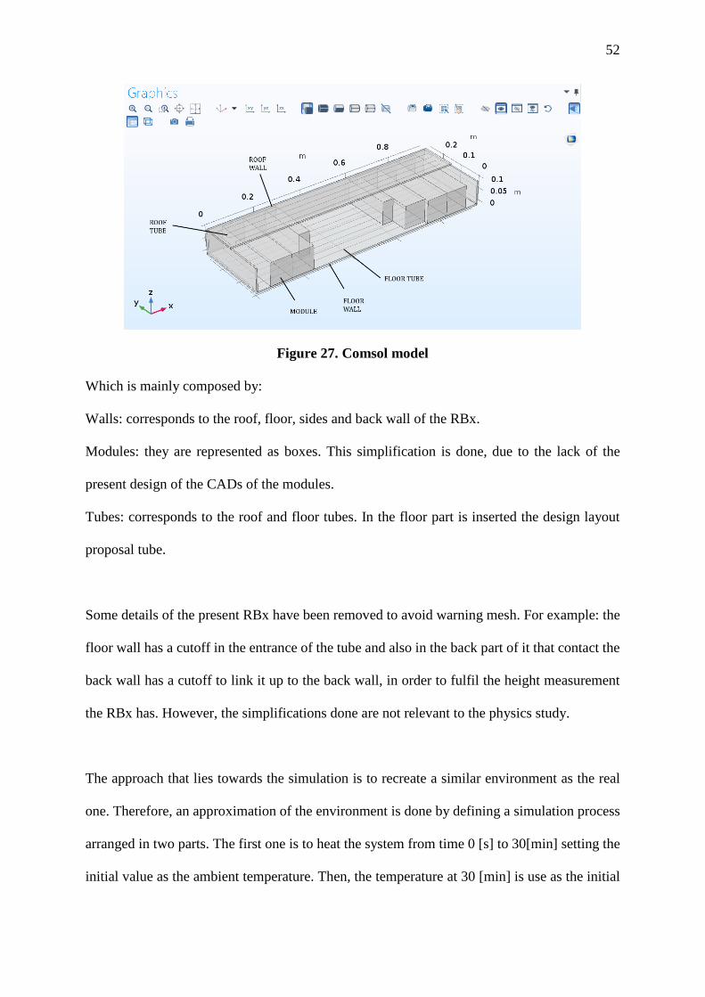
Figure 27. Comsol model
Which is mainly composed by:
Walls: corresponds to the roof, floor, sides and back wall of the RBx.
Modules: they are represented as boxes. This simplification is done, due to the lack of the
present design of the CADs of the modules.
Tubes: corresponds to the roof and floor tubes. In the floor part is inserted the design layout
proposal tube.
Some details of the present RBx have been removed to avoid warning mesh. For example: the
floor wall has a cutoff in the entrance of the tube and also in the back part of it that contact the
back wall has a cutoff to link it up to the back wall, in order to fulfil the height measurement
the RBx has. However, the simplifications done are not relevant to the physics study.
The approach that lies towards the simulation is to recreate a similar environment as the real
one. Therefore, an approximation of the environment is done by defining a simulation process
arranged in two parts. The first one is to heat the system from time 0 [s] to 30[min] setting the
initial value as the ambient temperature. Then, the temperature at 30 [min] is use as the initial
53
condition for the following part. The second part cools down the system for 5 [min] and in
consequence another distribution temperature exists in the system. Both parts in Comsol are
set as transient studies. Further, the selection of the most appropriate cooling proposal tube
layout is the one which lowers the system temperature more.
The detail of the steps set up in Comsol Multiphysics for the model are show below. In the
physics and follow steps, it is established a sequence with numbers to provide a guide of how
each node is define.
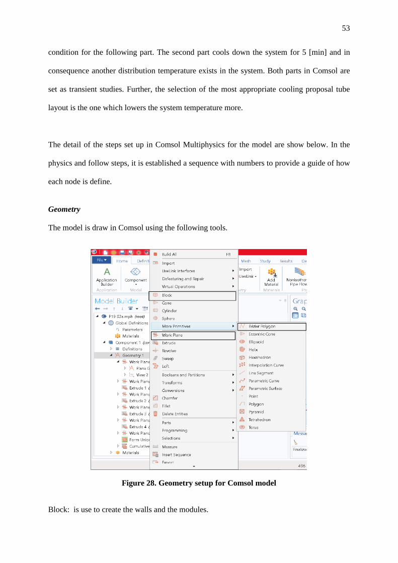
Geometry The model is draw in Comsol using the following tools.
Figure 28. Geometry setup for Comsol model
Block: is use to create the walls and the modules.
54
Work plane: is use to create independent parts, but are related to a common plane.
Bezier polygon: is use to create the 1D curves for the tubes.
The model is design to only insert a new tube layout proposal and keep everything the same.
So as not to have draw every time the layout change.
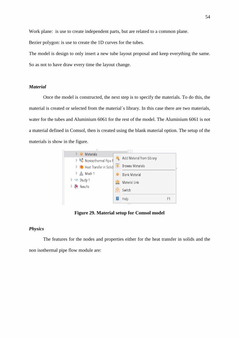
Material
Once the model is constructed, the next step is to specify the materials. To do this, the
material is created or selected from the material´s library. In this case there are two materials,
water for the tubes and Aluminium 6061 for the rest of the model. The Aluminium 6061 is not
a material defined in Comsol, then is created using the blank material option. The setup of the
materials is show in the figure.
Figure 29. Material setup for Comsol model
Physics
The features for the nodes and properties either for the heat transfer in solids and the
non isothermal pipe flow module are:

55
Heat Transfer in solids module setup
Figure 30. Heat transfer in solids module setup for Comsol model
In the heat transfer in solids node #1 is set as default. The solid node #2 specifies the
RBx as solid with the temperature (𝑇𝑇ℎ𝑜𝑜) and link the properties defined in the materials section.
In the initial values node # 3, it is specified the ambient temperature set up in node #1. This
corresponds to the initial condition of the system at time 0 [s]. The thermal insulation is set as
default. And at last, the heat source node #5 specifies the heat load per module according to
figure 16.
56
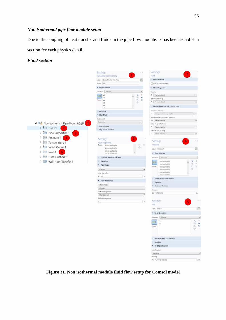
Non isothermal pipe flow module setup
Due to the coupling of heat transfer and fluids in the pipe flow module. Is has been establish a
section for each physics detail.
Fluid section
Figure 31. Non isothermal module fluid flow setup for Comsol model
57
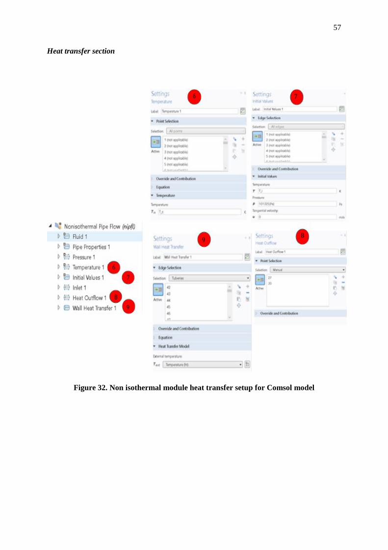
Heat transfer section
Figure 32. Non isothermal module heat transfer setup for Comsol model

58
Mesh setup
The mesh is user defined, where is divide by the elements section: edge for the 1D tube curves
and free tetrahedral for the rest of the geometry. It is set as follows:
Figure 33. Mesh setup for Comsol model

59
Study setup
In the study section, is composed of two steps. The first step considers the heat transient study
without the presence of the working fluid. The second step activates the cooling system [check
box] and uses the solution of the first step [values of dependent section].
Figure 34. Study setup for Comsol model
In this way the system is setup for the analysis.
60
3. RESULTS AND DISCUSSION
3.1 Mathematical Results
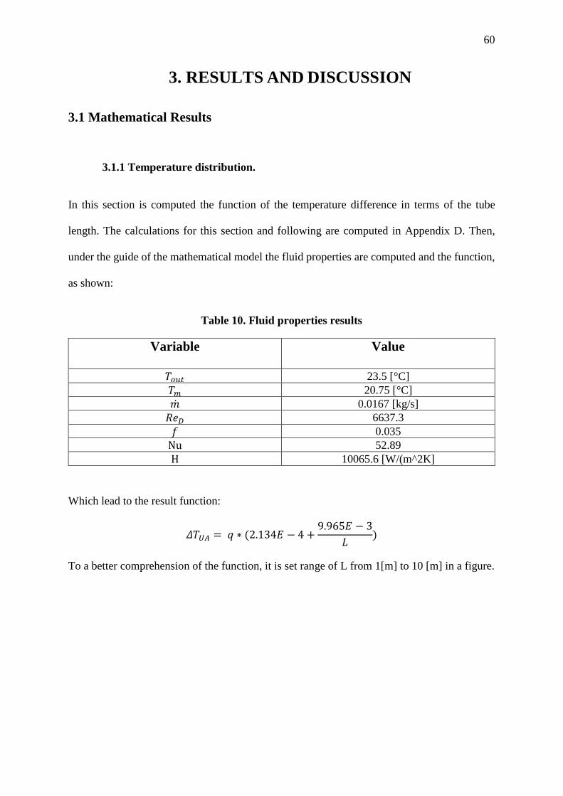
3.1.1 Temperature distribution.
In this section is computed the function of the temperature difference in terms of the tube
length. The calculations for this section and following are computed in Appendix D. Then,
under the guide of the mathematical model the fluid properties are computed and the function,
as shown:
Table 10. Fluid properties results
Variable
Value
𝑇𝑇𝑜𝑜𝑜𝑜𝑜𝑜 23.5 [°C] 𝑇𝑇𝑚𝑚 20.75 [°C] �̇�𝑚 0.0167 [kg/s] 𝑅𝑅𝑅𝑅𝐷𝐷 6637.3 𝑓𝑓 0.035
Nu 52.89 H 10065.6 [W/(m^2K]
Which lead to the result function:
𝛥𝛥𝑇𝑇𝑈𝑈𝑈𝑈 = 𝑞𝑞 ∗ (2.134𝐸𝐸 − 4 +9.965𝐸𝐸 − 3
𝐿𝐿)
To a better comprehension of the function, it is set range of L from 1[m] to 10 [m] in a figure.
61
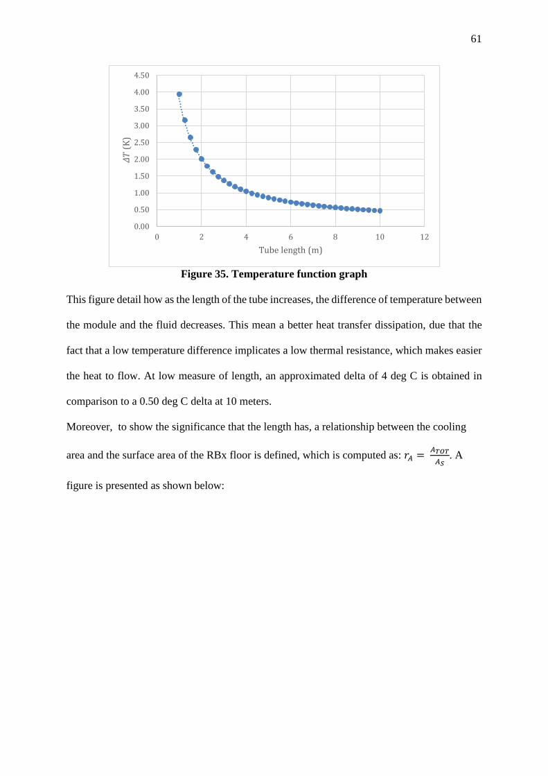
Figure 35. Temperature function graph
This figure detail how as the length of the tube increases, the difference of temperature between
the module and the fluid decreases. This mean a better heat transfer dissipation, due that the
fact that a low temperature difference implicates a low thermal resistance, which makes easier
the heat to flow. At low measure of length, an approximated delta of 4 deg C is obtained in
comparison to a 0.50 deg C delta at 10 meters.
Moreover, to show the significance that the length has, a relationship between the cooling
area and the surface area of the RBx floor is defined, which is computed as: 𝑃𝑃𝑈𝑈 = 𝑈𝑈𝑇𝑇𝑇𝑇𝑇𝑇𝑈𝑈𝑆𝑆
. A
figure is presented as shown below:
0.00
0.50
1.00
1.50
2.00
2.50
3.00
3.50
4.00
4.50
0 2 4 6 8 10 12
𝛥𝛥𝑇𝑇(K
)
Tube length (m)

62
Figure 36. Relationship between cooling area and temperature
It details that a lower temperature difference is obtained by a low relationship proportion of the
𝑃𝑃𝑈𝑈, meaning that the cooling area is bigger, and more heat can be dissipated, justify it by
Newtown’s law.
3.1.2 Pipe friction losses.
In this section is computed the pressure losses that the fluid experiences. It is focus on how
major losses and minor losses affect it, to demonstrate a figure of delta pressure is graph.
Hence, it is obtained a mean velocity of �𝑣𝑣 = 2.11 �𝑚𝑚𝑠𝑠�� and a bending k factor due to a 90-
degree bend in a turbulent flow of (𝐾𝐾𝑅𝑅 = 0.323). Considering this results and equation of
Bernouilli, the given function of pressure difference in terms of length is obtained.
𝛥𝛥𝑝𝑝 = [0.227(0.035 ∗ 𝐿𝐿
3.175𝐸𝐸 − 3+ 𝑛𝑛 ∗ 0.323)](9810)
0.00
0.50
1.00
1.50
2.00
2.50
3.00
3.50
4.00
4.50
0 5 10 15 20 25 30 35
𝛥𝛥𝑇𝑇(K
)
r_A

63
The function is graph by setting different number of bends (n) in the range of 1-80 bends and
a length range from 1-10 [m].
Figure 37. Pressure change in function of length and number of lengths
It is show that in a general overview, the major losses have a significance value more than the
minor losses. The effect of the bend is considerable but not as the friction between the pipe and
the fluid. A maximum change of pressure from 1 bend to 80 bends considering at 1-10 [m],
gives approximate 0.60 (atm), however, the change of pressure from 1-10[m] by the length of
the tube gives approximate 2.18 (atm).
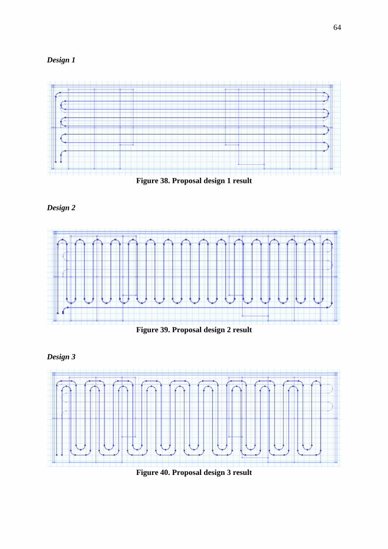
3.2 Tube layout results
In this section is presented the layout proposal designs results. This overview the results
variables and the layout design drawings for each case in COMSOL. At last, the total length of
the tube layout is presented.
0.00
0.50
1.00
1.50
2.00
2.50
3.00
3.50
0 2 4 6 8 10 12
𝛥𝛥P(a
tm)
Length (m)
1
10
20
30
40
50
60
70
80
n
64
Design 1
Figure 38. Proposal design 1 result
Design 2
Figure 39. Proposal design 2 result
Design 3
Figure 40. Proposal design 3 result

65
Table 11. Length per design
Design Length (m) 1 7.79 2 8.43 3 10.21
As shown, despite having the same bend diameter, it is obtained that the type of distribution
enables to obtain more or less tube length.
3.3 Simulation Results
This section is divided in two parts: qualitative results and quantitative results.
3.3.1 Qualitative results.
The qualitative results overview the results from the initial condition of the system and present
design temperature distribution. Moreover, in order to compare results, the temperature and
heat flux distribution is shown, the floor distribution and a selected module for each design
proposal.
The initial condition of the system before the activation of the cooling system, is show below:
Figure 41. Initial temperature distribution of the system at t = 30 [min]
At first glance, the temperature distribution in the RBx is not uniform due that the heat
generation in the left side is higher than the right side. So then, a higher temperature is expected
where more heat is generated.
66
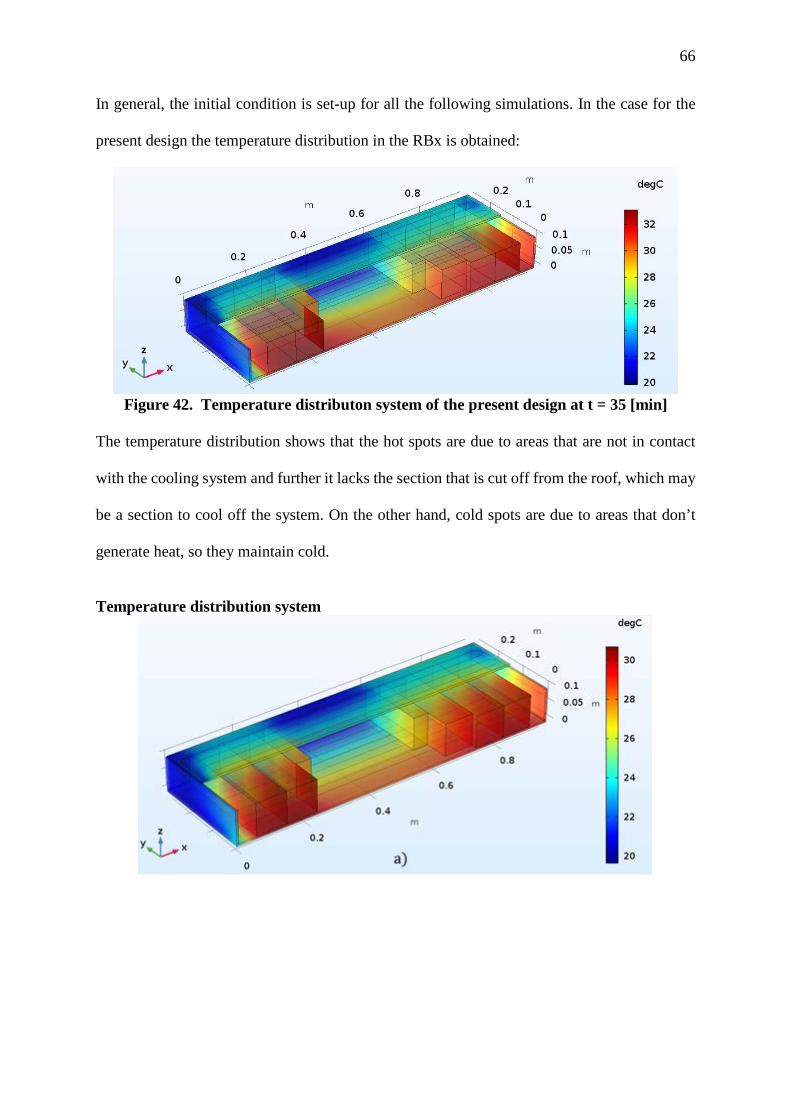
In general, the initial condition is set-up for all the following simulations. In the case for the
present design the temperature distribution in the RBx is obtained:
Figure 42. Temperature distributon system of the present design at t = 35 [min]
The temperature distribution shows that the hot spots are due to areas that are not in contact
with the cooling system and further it lacks the section that is cut off from the roof, which may
be a section to cool off the system. On the other hand, cold spots are due to areas that don’t
generate heat, so they maintain cold.
Temperature distribution system

67
Figure 43. Temperature distribution system at t = 35 [min] a). Design 1
b) Design 2. c) Design 3.
In this figure it can be seen that the distribution temperature is different for each proposal
design. The first design has a similar distribution to the present design, because it has the same
distribution but with more bends. The second design in comparison with the first one, shows
lower temperatures on the left side than the right side, due to the increase of quantity of the
cooling system area (length of tube), the same applied between the third design and the first.
In the second and third design, the temperature is higher in the right side, because as the fluid
advances it gains heat and its temperature increases, then, the heat transfer decreases.
68
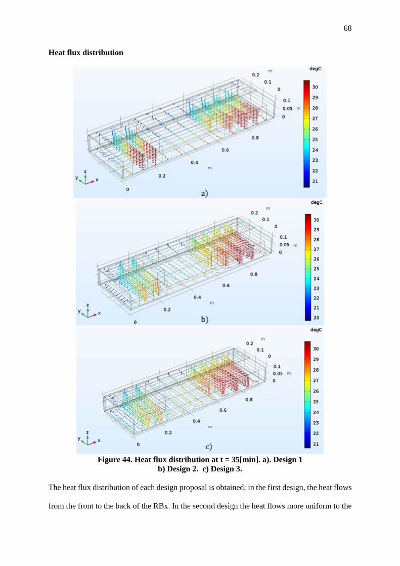
Heat flux distribution
Figure 44. Heat flux distribution at t = 35[min]. a). Design 1
b) Design 2. c) Design 3.
The heat flux distribution of each design proposal is obtained; in the first design, the heat flows
from the front to the back of the RBx. In the second design the heat flows more uniform to the
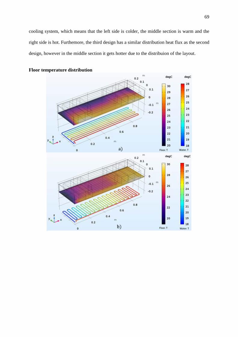
69
cooling system, which means that the left side is colder, the middle section is warm and the
right side is hot. Furthemore, the third design has a similar distribution heat flux as the second
design, however in the middle section it gets hotter due to the distribuion of the layout.
Floor temperature distribution
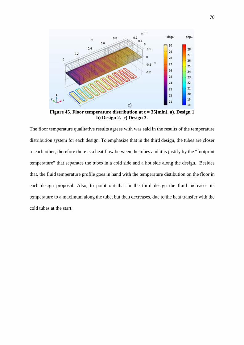
70
Figure 45. Floor temperature distribution at t = 35[min]. a). Design 1
b) Design 2. c) Design 3.
The floor temperature qualitative results agrees with was said in the results of the temperature
distribution system for each design. To emphasize that in the third design, the tubes are closer
to each other, therefore there is a heat flow between the tubes and it is justify by the “footprint
temperature” that separates the tubes in a cold side and a hot side along the design. Besides
that, the fluid temperature profile goes in hand with the temperature distibution on the floor in
each design proposal. Also, to point out that in the third design the fluid increases its
temperature to a maximum along the tube, but then decreases, due to the heat transfer with the
cold tubes at the start.

71
Module 1 temperature distribution
Figure 46. Module 1 temperature distribution at t = 35[min]. a). Design 1
b) Design 2. c) Design 3.
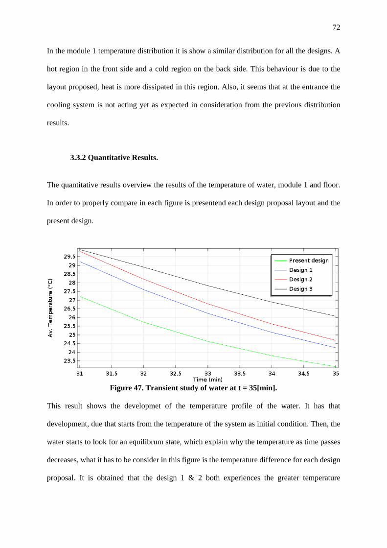
72
In the module 1 temperature distribution it is show a similar distribution for all the designs. A
hot region in the front side and a cold region on the back side. This behaviour is due to the
layout proposed, heat is more dissipated in this region. Also, it seems that at the entrance the
cooling system is not acting yet as expected in consideration from the previous distribution
results.
3.3.2 Quantitative Results.
The quantitative results overview the results of the temperature of water, module 1 and floor.
In order to properly compare in each figure is presentend each design proposal layout and the
present design.
Figure 47. Transient study of water at t = 35[min].
This result shows the developmet of the temperature profile of the water. It has that
development, due that starts from the temperature of the system as initial condition. Then, the
water starts to look for an equilibrum state, which explain why the temperature as time passes
decreases, what it has to be consider in this figure is the temperature difference for each design
proposal. It is obtained that the design 1 & 2 both experiences the greater temperature
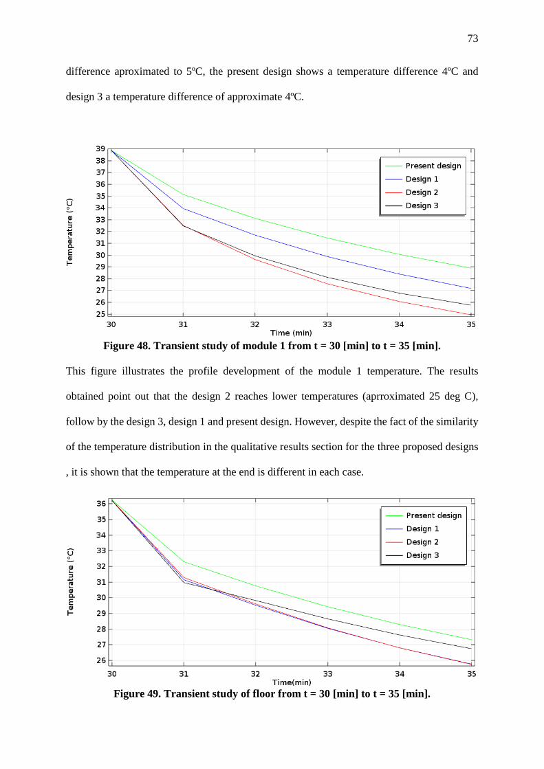
73
difference aproximated to 5ºC, the present design shows a temperature difference 4ºC and
design 3 a temperature difference of approximate 4ºC.
Figure 48. Transient study of module 1 from t = 30 [min] to t = 35 [min].
This figure illustrates the profile development of the module 1 temperature. The results
obtained point out that the design 2 reaches lower temperatures (aprroximated 25 deg C),
follow by the design 3, design 1 and present design. However, despite the fact of the similarity
of the temperature distribution in the qualitative results section for the three proposed designs
, it is shown that the temperature at the end is different in each case.
Figure 49. Transient study of floor from t = 30 [min] to t = 35 [min].

74
This figure illustrates the temperature profile of the floor. The results obtained point out that
design 1 & 2 reaches the lower temperatures (aprroximated 26ºC both) than the present design
and design 3. This corroborate with the qualitative results obtained of the temperature
distribution of the floor, that both design 1 & design 2 experiences a better heat dissipation rate
to the cooling system than the other layouts.
Having the results for all the proposed designs, the centralized weight method can be applied
to select the correct design layout. The criteria consider for the method are those that are
relevant to accomplish the features required for the cooling system. The criteria selected
are:heat dissipation (HD) , construction viability (CV) , cost (CST) and fluid control (FC). The
results are presented in the following table.
Table 12. Centralized weight method
CRITERIA
DESIGN HD (5) FEA (5) CST (3) FC (3) ∑▒+1 Result
1 4 5 3 3 16 1,6
2 5 5 2 2 15 1,5
3 4 3 1 1 9,5 0,95
10 1
The given score for each criteria agrees with the degree of importance that the criteria has on
the specifications. So, the heat dissipation and the feasibility have a higher value, due that both
criteria are the main objectives of the working project than the cost and fluid control. However,
that does not mean that the remaining criteria are negligible.

75
It is determined due to the closeness of the results from the centralized weight method, both
design 1 & 2 are selected. Then, the future work will test both designs to properly select the
correct one.
76
4. CONCLUSION AND RECOMMENDATIONS
In conclusion, a new distribution of the pipe was achieved; which is feasible to carry out
for a future construction. Firstly, it is determined that the tube layout is a remarkable design
factor to consider, since the length of the tube is not enough to ensure a greater heat transfer as
shown on the floor temperature distribution (Figure 45) and justify it by the quantitative results
from figure 49. Moreover, a simulation model was set-up in Comsol Multiphysics that allowed
to simulate the operating conditions of the RBx. Then, in the simulation results the three types
of proposal designs were compare , where it was obtained that the second design demostrate
better perfomance as a cooling system. However, when the centralized weigth method is
consider , the first design also became one of the selected options due to the results obtained.
In general, the selected proposal designs accomplish to reduce the temperature of the floor of
the RBx to approximate 26ºC. Nevertheless, both designs obtained greater temperature
difference of water by approximated 5ºC.
As recommendations of this senior thesis, it is suggested to use the same modules of
heat transfer in solids and non-isothermal pipe flow, since that avoids waste of time and
inneficient results. Further, if another refrigerant want to be use, the same procedure is
maintained; just change the set-up in the material section to specify the fluid type and
properties. To finalyze, the implementation of the updated CADs of the modules will help to
obtain more realistic results.

77
5. FUTURE WORK
The work done corresponds to the first part of this global project, the preliminary phase. In
which the designs over the system were coupling by simulation. The next phase follows the
construction of the prototype to evaluate experimentally the results, in order to validate the
results from the simulation and compare them. Therefore, the following experimental setup to
study the different cooper line distribution layouts is established, as shown in figure 50.
Figure 50. Experimental setup of the prototype cooling system.
Considering the previous experimental setup a projected budget for the construction is
proposed; considering it will be constructed in Ecuador.
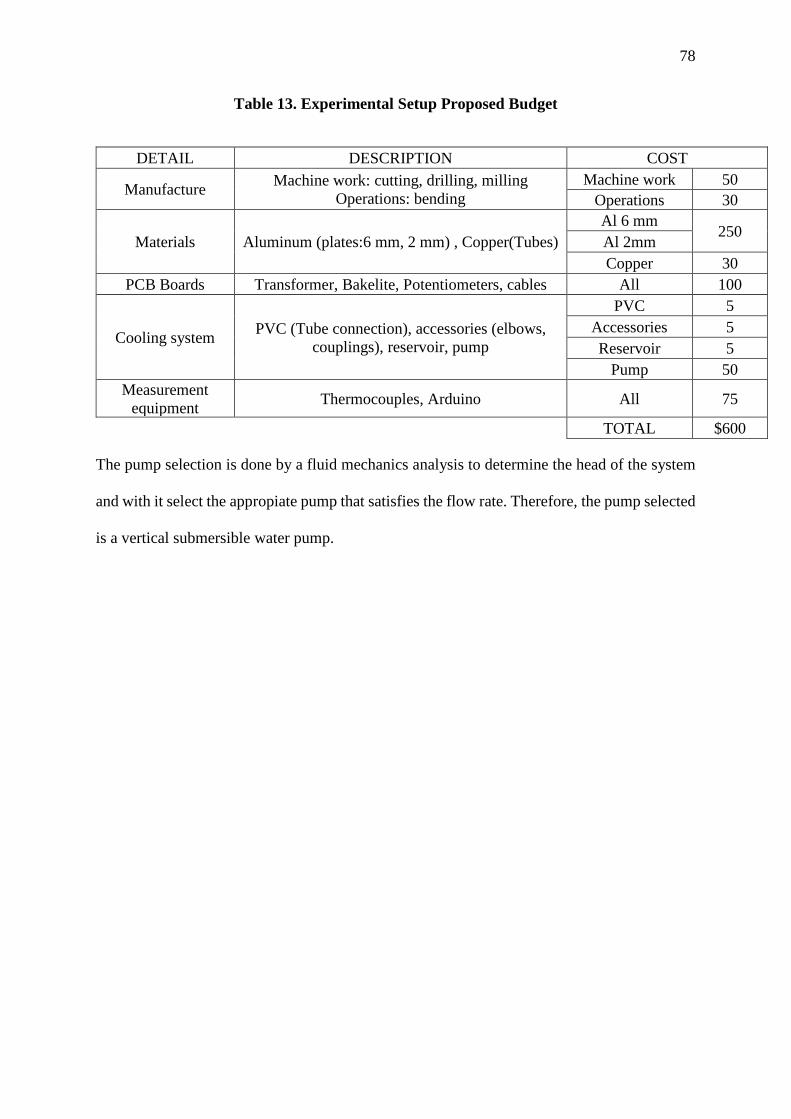
78
Table 13. Experimental Setup Proposed Budget
DETAIL DESCRIPTION COST
Manufacture Machine work: cutting, drilling, milling Operations: bending
Machine work 50 Operations 30
Materials Aluminum (plates:6 mm, 2 mm) , Copper(Tubes) Al 6 mm
250 Al 2mm Copper 30
PCB Boards Transformer, Bakelite, Potentiometers, cables All 100
Cooling system PVC (Tube connection), accessories (elbows, couplings), reservoir, pump
PVC 5 Accessories 5 Reservoir 5
Pump 50 Measurement
equipment Thermocouples, Arduino All 75
TOTAL $600
The pump selection is done by a fluid mechanics analysis to determine the head of the system
and with it select the appropiate pump that satisfies the flow rate. Therefore, the pump selected
is a vertical submersible water pump.
79
6. REFERENCES
CERN Geneva The LHC experiments Committee. (2017). The Phase-2 Upgrade of the CMS
Barrel Calorimeters TDR. Retrieved from
https://cds.cern.ch/record/2283187/files/CMS-TDR-015.pdf
CERN Geneva The LHC Experiments Committee. (1997). HCAL TDR. Retrieved from
https://cds.cern.ch/record/357153/files/CMS_HCAL_TDR.pdf
INSTITUTE OF PHYSICS PUBLISHING AND SISSA. (2008). The CMS experiment at the
CERN LHC (Vol. 3). https://doi.org/10.1088/1748-0221/3/08/S08004
Karmgard, D. (2001). RBX Cooling. Retrieved July 4, 2018, from
http://physics.bu.edu/cms/hcal/RBX_PRR/prr-cooling.ppt
Mans, J. (2012). CMS TDR for the Phase 1 Upgrade of the Hadron Calorimeter. Retrieved
from http://cds.cern.ch/record/1481837/files/CMS-TDR-010.pdf
Ruchti, R. (2001). HCAL RBX for HB HE and HO Status and Planning. Retrieved July 4,
2018, from http://physics.bu.edu/cms/hcal/RBX_PRR/RR PRR talk for 3-1-01 updated
2-24-01.ppt
Schmidt, I. (2018). HB RBX Introduction Ecuador.
Incropera, F. P. and DeWitt, D. P. (2011). Fundamentals of Heat and Mass Transfer. United
States, New York: John Wiley and Sons , Inc
Barney, D. (2003). An overview of the CMS experiment for CERN guides. Retrieved from
https://cds.cern.ch/record/2283187/files/CMS-TDR-015.pdf
Huc, N. (2014) .Conjugate heat transfer. Retrieved July 17, 2018, from
https://www.comsol.com/blogs/conjugate-heat-transfer/
Wollblad, C. (2017). CFD in Comsol Multiphysics. Retrieved from
https://www.kth.se/social/files/591470ecf276542fd65c9a1e/kth170510.pdf
COMSOL. (2014). Comsol Multiphysics User's Guide. Retrieved from
http://people.ee.ethz.ch/~fieldcom/pps-
comsol/documents/User%20Guide%20and%20Examples/COMSOLMultiphysicsUsers
Guide.pdf
COMSOL. (2012). Pipe flow module User's Guide. Retrieved from
http://people.ee.ethz.ch/~fieldcom/pps-
comsol/documents/User%20Guide%20and%20Examples/COMSOLMultiphysicsUsers
Guide.pdf

80
Copper Development Association. (2017). Copper Tube Handbook. Retrieved from
https://www.copper.org/publications/pub_list/pdf/copper_tube_handbook.pdf
YORKSHIRE. (2014). TECHNICAL GUIDE. Retrieved from http://yorkshirecopper.com/wp-
content/uploads/Technical-Guide-full-issue-02_14_Really2.pdf
CAE ASSOCIATES. (2009). Heat Exchanger Cooling Analysis. Retrieved from
https://caeai.com/sites/default/files/Heat%20Exchanger%20Cooling%20Analysis.pdf
Yang, J. (2009). Heat Transfer coefficient in flow convection of pipe cooling system in massive
concrete. Retrieved from https://www.jstage.jst.go.jp/article/jact/9/1/9_1_103/_article
Aalco. (2018). Aluminium Alloy 6061- T6 Extrusions. Retrieved from
http://www.aalco.co.uk/datasheets/?search=al%206061%20t6
Efunda. (2007). Absolute pipe roughness. Retrieved from
http://www.efunda.com/formulae/fluids/roughness.cfm
Munson, B. (2009). Fundamentals of Fluid Mechanics. United States, Jefferson City: John
Wiley and Sons , Inc
RIDGID. (2013). BENDING & FORMING. Retrieved from
http://www.ridgid.eu/catalog/EN/08_Bending_EN_WEB.pdf
White, F. (2011). Fluids Mechanics. United States, New York: Mc Graw Hill
CMS DocDB Administrators (2001). List of topics. Retrieved from https://cms-
docdb.cern.ch/cgi-bin/DocDB/DocumentDatabase

81
7. APPENDIX
7.1 Appendix A
Table A.1. Water properties (Incropera, 2011)
Table A.2. Aluminum 6061 properties (Aalco,2018)
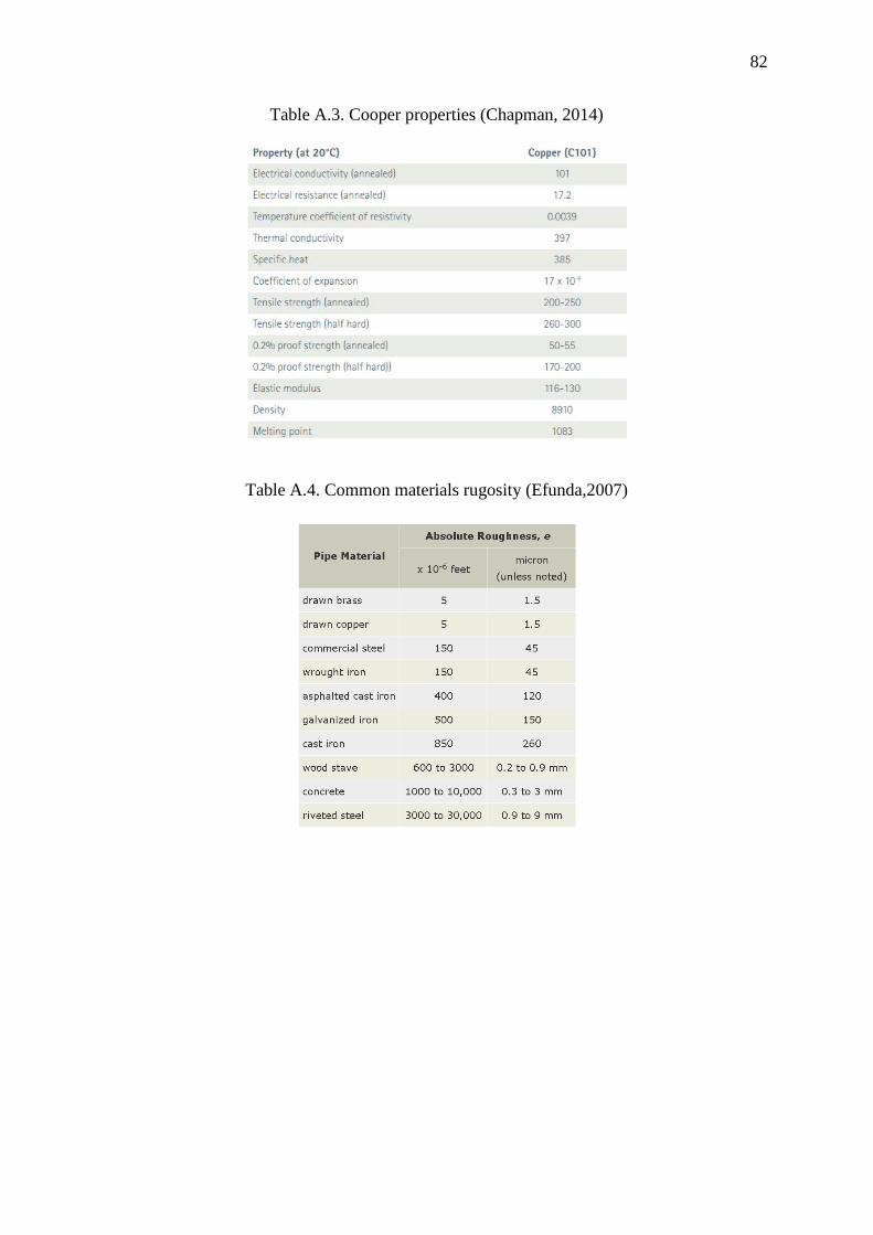
82
Table A.3. Cooper properties (Chapman, 2014)
Table A.4. Common materials rugosity (Efunda,2007)
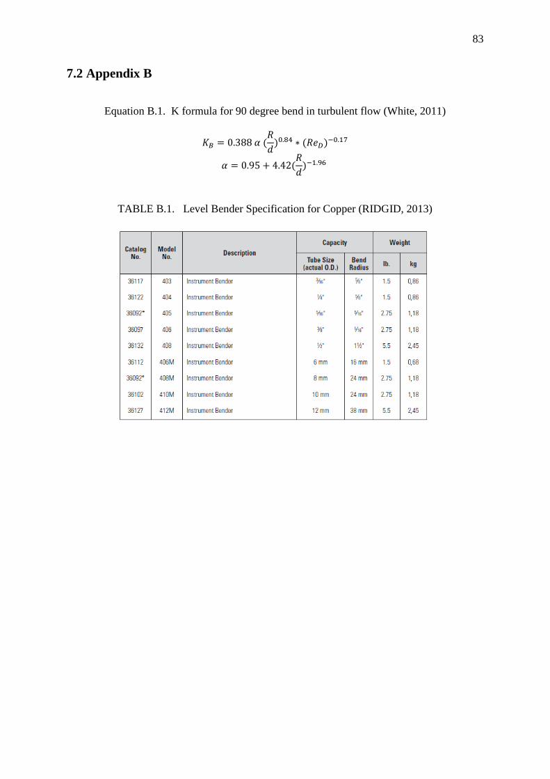
83
7.2 Appendix B
Equation B.1. K formula for 90 degree bend in turbulent flow (White, 2011)
𝐾𝐾𝑅𝑅 = 0.388 𝛼𝛼 (𝑅𝑅𝑑𝑑
)0.84 ∗ (𝑅𝑅𝑅𝑅𝐷𝐷)−0.17
𝛼𝛼 = 0.95 + 4.42(𝑅𝑅𝑑𝑑
)−1.96
TABLE B.1. Level Bender Specification for Copper (RIDGID, 2013)
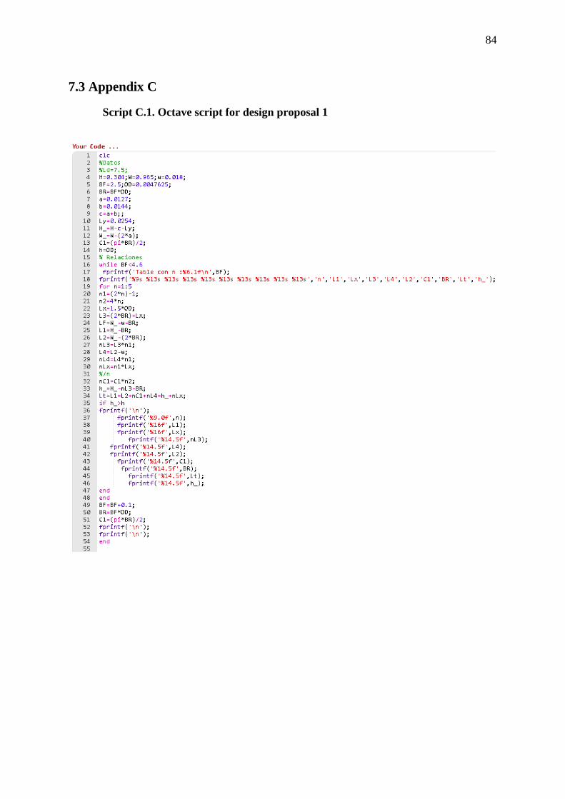
84
7.3 Appendix C
Script C.1. Octave script for design proposal 1
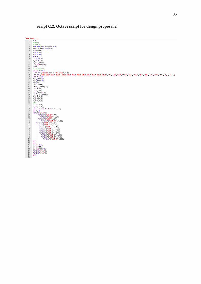
85
Script C.2. Octave script for design proposal 2
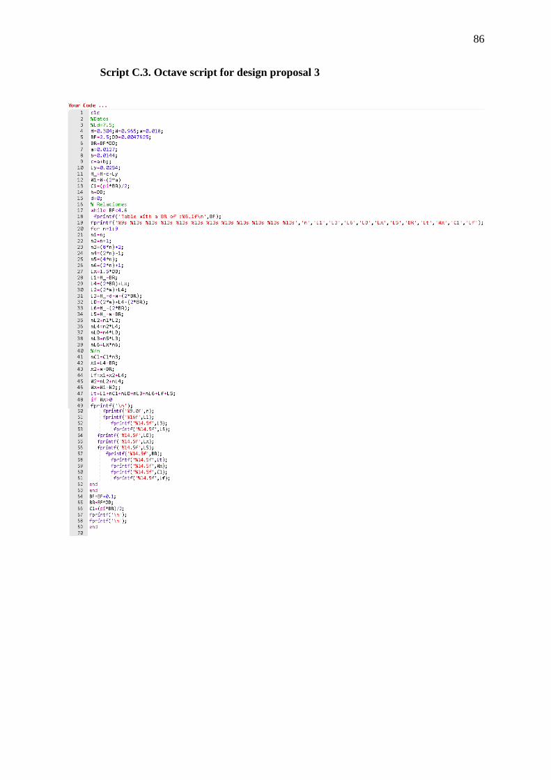
86
Script C.3. Octave script for design proposal 3
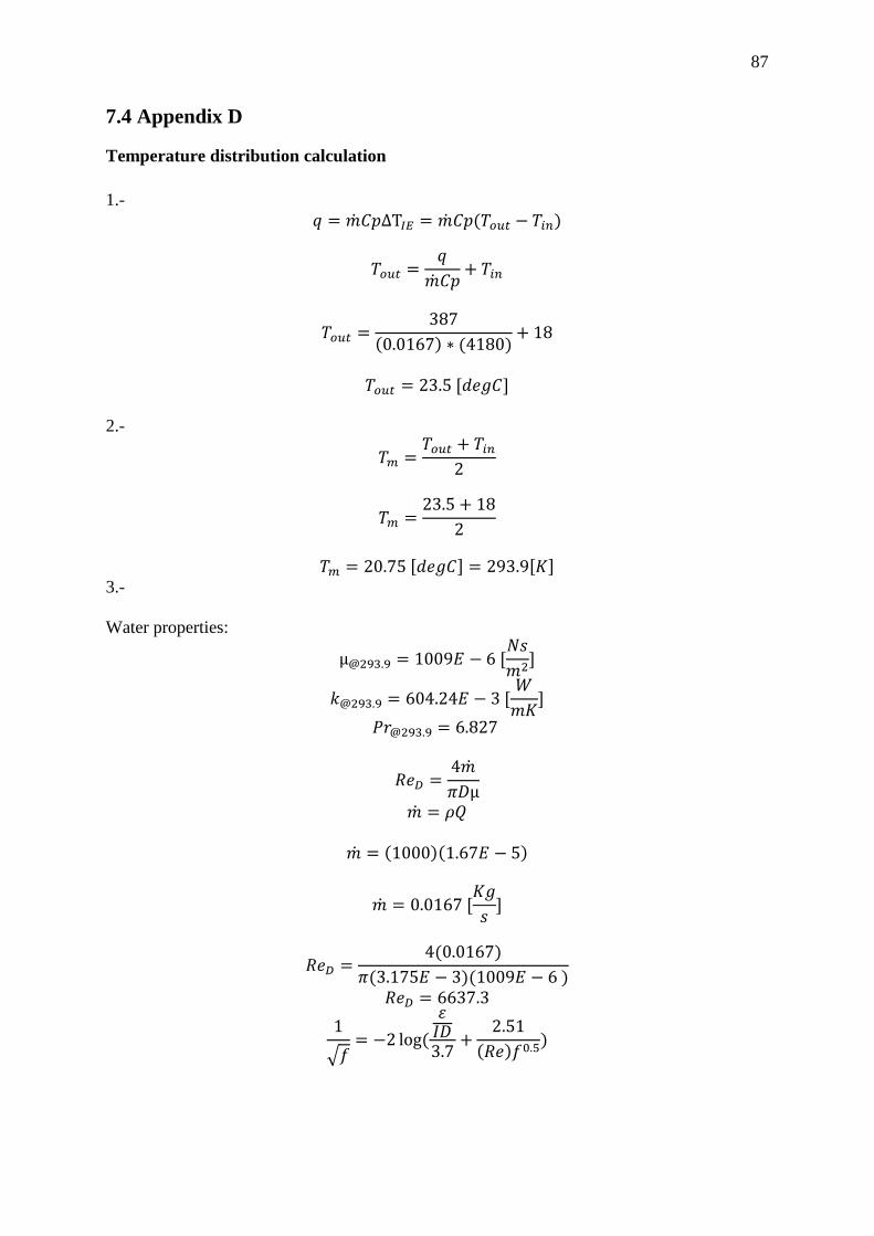
87
7.4 Appendix D
Temperature distribution calculation 1.-
𝑞𝑞 = �̇�𝑚𝐶𝐶𝑝𝑝ΔT𝐼𝐼𝐼𝐼 = �̇�𝑚𝐶𝐶𝑝𝑝(𝑇𝑇𝑜𝑜𝑜𝑜𝑜𝑜 − 𝑇𝑇𝑖𝑖𝑖𝑖)
𝑇𝑇𝑜𝑜𝑜𝑜𝑜𝑜 =𝑞𝑞
�̇�𝑚𝐶𝐶𝑝𝑝+ 𝑇𝑇𝑖𝑖𝑖𝑖
𝑇𝑇𝑜𝑜𝑜𝑜𝑜𝑜 =387
(0.0167) ∗ (4180)+ 18
𝑇𝑇𝑜𝑜𝑜𝑜𝑜𝑜 = 23.5 [𝑑𝑑𝑅𝑅𝑔𝑔𝐶𝐶]
2.-
𝑇𝑇𝑚𝑚 =𝑇𝑇𝑜𝑜𝑜𝑜𝑜𝑜 + 𝑇𝑇𝑖𝑖𝑖𝑖
2
𝑇𝑇𝑚𝑚 =23.5 + 18
2
𝑇𝑇𝑚𝑚 = 20.75 [𝑑𝑑𝑅𝑅𝑔𝑔𝐶𝐶] = 293.9[𝐾𝐾]
3.- Water properties:
µ@293.9 = 1009𝐸𝐸 − 6 [𝑁𝑁𝑁𝑁𝑚𝑚2]
𝑘𝑘@293.9 = 604.24𝐸𝐸 − 3 [𝑊𝑊𝑚𝑚𝐾𝐾
] 𝑃𝑃𝑃𝑃@293.9 = 6.827
𝑅𝑅𝑅𝑅𝐷𝐷 =4�̇�𝑚𝜋𝜋𝐷𝐷µ
�̇�𝑚 = 𝜌𝜌𝑄𝑄
�̇�𝑚 = (1000)(1.67𝐸𝐸 − 5)
�̇�𝑚 = 0.0167 [𝐾𝐾𝑔𝑔𝑁𝑁
]
𝑅𝑅𝑅𝑅𝐷𝐷 =4(0.0167)
𝜋𝜋(3.175𝐸𝐸 − 3)(1009𝐸𝐸 − 6 )
𝑅𝑅𝑅𝑅𝐷𝐷 = 6637.3 1�𝑓𝑓
= −2 log(𝜀𝜀𝐼𝐼𝐷𝐷3.7
+2.51
(𝑅𝑅𝑅𝑅)𝑓𝑓0.5)

88
1�𝑓𝑓
= −2 log(1.5𝐸𝐸 − 6
3.175𝐸𝐸 − 33.7
+2.51
(6637.3)𝑓𝑓0.5
Initial guess: 𝑓𝑓 = 0.02
1√0.02
= −2 log(1.5𝐸𝐸 − 6
3.175𝐸𝐸 − 33.7
+2.51
(6637.3)0.020.5
7.07 = 5.1
By iteration: 𝑓𝑓 = 0.035
𝑁𝑁𝑢𝑢 =�𝑓𝑓8� (𝑅𝑅𝑅𝑅𝐷𝐷 − 1000)𝑃𝑃𝑃𝑃
1 + 12.7 �𝑓𝑓8�12
(𝑃𝑃𝑃𝑃23 − 1)
𝑁𝑁𝑢𝑢 =�0.035
8 � (6637.3 − 1000)6.827
1 + 12.7 �0.0358 �
12
(6.82723 − 1)
𝑁𝑁𝑢𝑢 = 52.89
Nu =ℎ𝐷𝐷𝑘𝑘
h =𝑁𝑁𝑢𝑢𝑘𝑘𝐷𝐷
h =(52.89)(604.24𝐸𝐸 − 3)
(3.175𝐸𝐸 − 3)
h = 10065.6 [𝑊𝑊𝑚𝑚2𝐾𝐾
] 4.- Applied on the system, from the module temperature to the fluid temperature.
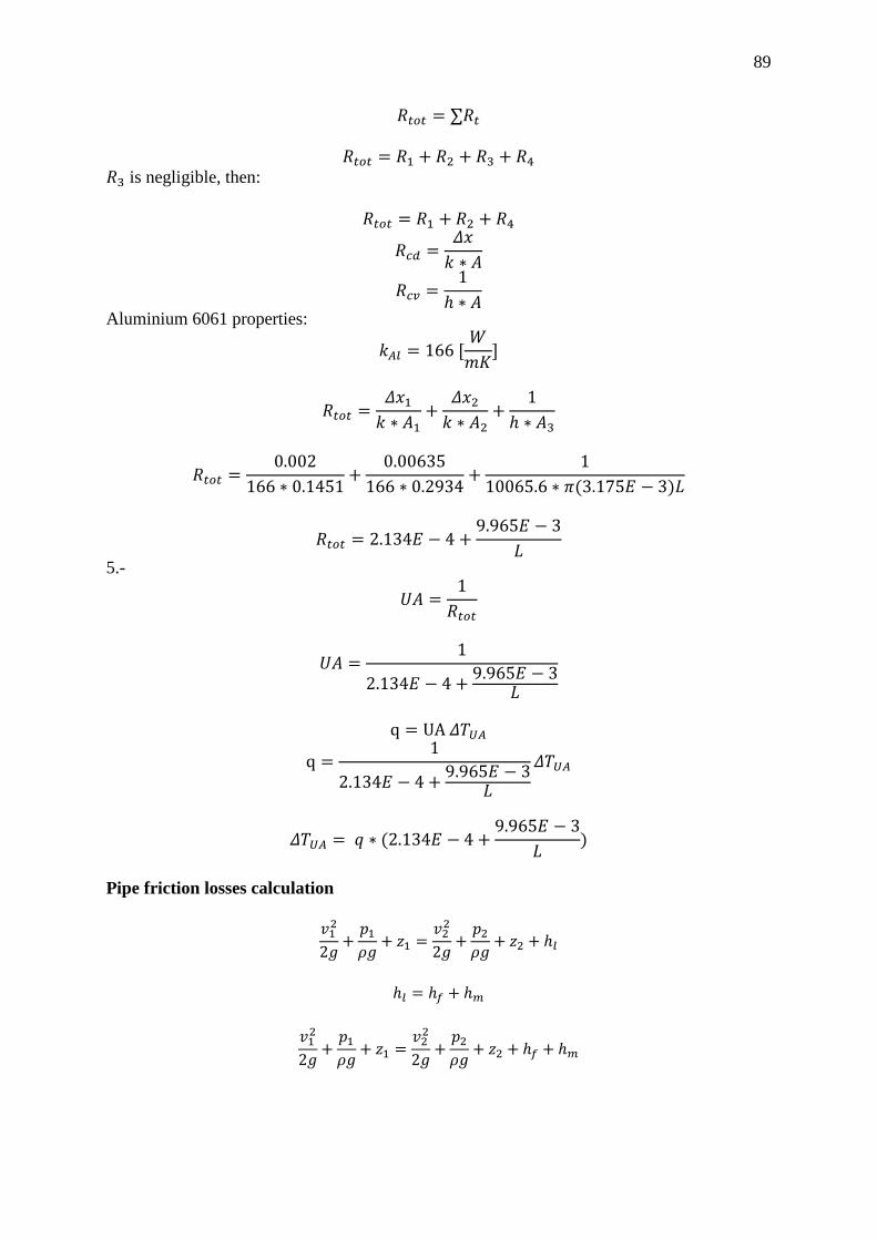
89
𝑅𝑅𝑜𝑜𝑜𝑜𝑜𝑜 = ∑𝑅𝑅𝑜𝑜
𝑅𝑅𝑜𝑜𝑜𝑜𝑜𝑜 = 𝑅𝑅1 + 𝑅𝑅2 + 𝑅𝑅3 + 𝑅𝑅4 𝑅𝑅3 is negligible, then:
𝑅𝑅𝑜𝑜𝑜𝑜𝑜𝑜 = 𝑅𝑅1 + 𝑅𝑅2 + 𝑅𝑅4
𝑅𝑅𝑐𝑐𝑐𝑐 =𝛥𝛥𝑑𝑑𝑘𝑘 ∗ 𝐴𝐴
𝑅𝑅𝑐𝑐𝑐𝑐 =1
ℎ ∗ 𝐴𝐴
Aluminium 6061 properties:
𝑘𝑘𝑈𝑈𝑙𝑙 = 166 [𝑊𝑊𝑚𝑚𝐾𝐾
]
𝑅𝑅𝑜𝑜𝑜𝑜𝑜𝑜 =𝛥𝛥𝑑𝑑1𝑘𝑘 ∗ 𝐴𝐴1
+𝛥𝛥𝑑𝑑2𝑘𝑘 ∗ 𝐴𝐴2
+1
ℎ ∗ 𝐴𝐴3
𝑅𝑅𝑜𝑜𝑜𝑜𝑜𝑜 =0.002
166 ∗ 0.1451+
0.00635166 ∗ 0.2934
+1
10065.6 ∗ 𝜋𝜋(3.175𝐸𝐸 − 3)𝐿𝐿
𝑅𝑅𝑜𝑜𝑜𝑜𝑜𝑜 = 2.134𝐸𝐸 − 4 +9.965𝐸𝐸 − 3
𝐿𝐿
5.-
𝑈𝑈𝐴𝐴 =1𝑅𝑅𝑜𝑜𝑜𝑜𝑜𝑜
𝑈𝑈𝐴𝐴 =1
2.134𝐸𝐸 − 4 + 9.965𝐸𝐸 − 3𝐿𝐿
q = UA 𝛥𝛥𝑇𝑇𝑈𝑈𝑈𝑈
q =1
2.134𝐸𝐸 − 4 + 9.965𝐸𝐸 − 3𝐿𝐿
𝛥𝛥𝑇𝑇𝑈𝑈𝑈𝑈
𝛥𝛥𝑇𝑇𝑈𝑈𝑈𝑈 = 𝑞𝑞 ∗ (2.134𝐸𝐸 − 4 +9.965𝐸𝐸 − 3
𝐿𝐿)
Pipe friction losses calculation
𝑣𝑣12
2𝑔𝑔+𝑝𝑝1𝜌𝜌𝑔𝑔
+ 𝑑𝑑1 =𝑣𝑣22
2𝑔𝑔+𝑝𝑝2𝜌𝜌𝑔𝑔
+ 𝑑𝑑2 + ℎ𝑙𝑙
ℎ𝑙𝑙 = ℎ𝑓𝑓 + ℎ𝑚𝑚
𝑣𝑣12
2𝑔𝑔+𝑝𝑝1𝜌𝜌𝑔𝑔
+ 𝑑𝑑1 =𝑣𝑣22
2𝑔𝑔+𝑝𝑝2𝜌𝜌𝑔𝑔
+ 𝑑𝑑2 + ℎ𝑓𝑓 + ℎ𝑚𝑚

90
ℎ𝑚𝑚 =𝑘𝑘𝑣𝑣2
2𝑔𝑔
ℎ𝑓𝑓 =𝑓𝑓𝐿𝐿𝑣𝑣2
𝐷𝐷2𝑔𝑔
𝛥𝛥𝑝𝑝𝜌𝜌𝑔𝑔
=𝑣𝑣2
2𝑔𝑔(𝑓𝑓𝐿𝐿𝐷𝐷
+ ∑𝐾𝐾𝑅𝑅)
1.- By using equation B.1:
𝐾𝐾𝑅𝑅 = 0.388 𝛼𝛼 (𝑅𝑅𝑑𝑑
)0.84 ∗ (𝑅𝑅𝑅𝑅𝐷𝐷)−0.17
𝛼𝛼 = 0.95 + 4.42(𝑅𝑅𝑑𝑑
)−1.96
𝑅𝑅𝑑𝑑
=19323
16
𝑅𝑅𝑑𝑑
= 3.167
This result is then used to select the correct 𝐾𝐾𝑅𝑅 to use. In order to do this, the equation of 𝐾𝐾𝑅𝑅 is
graph in the range of 1- 15 [R/d] to show how the factor is affected by the relationship.
Figure D1. Bending factor graph Furthermore, by using the figure D.1:
𝐾𝐾𝑅𝑅 = 0.323 2.-
𝑄𝑄 = 𝑣𝑣 ∗ 𝐴𝐴
𝑣𝑣 =𝑄𝑄𝐴𝐴
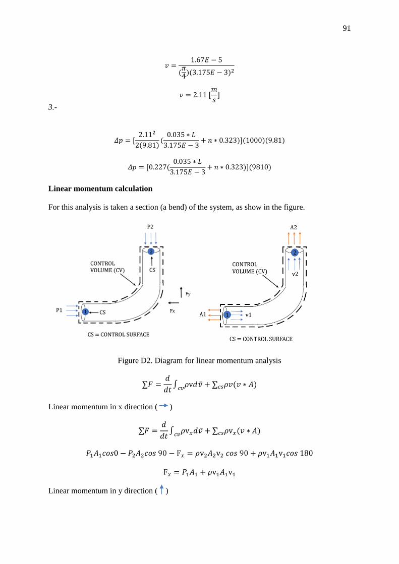
91
𝑣𝑣 =1.67𝐸𝐸 − 5
(𝜋𝜋4)(3.175𝐸𝐸 − 3)2
𝑣𝑣 = 2.11 [
𝑚𝑚𝑁𝑁
]
3.-
𝛥𝛥𝑝𝑝 = [2.112
2(9.81) (0.035 ∗ 𝐿𝐿
3.175𝐸𝐸 − 3+ 𝑛𝑛 ∗ 0.323)](1000)(9.81)
𝛥𝛥𝑝𝑝 = [0.227(0.035 ∗ 𝐿𝐿
3.175𝐸𝐸 − 3+ 𝑛𝑛 ∗ 0.323)](9810)
Linear momentum calculation For this analysis is taken a section (a bend) of the system, as show in the figure.
Figure D2. Diagram for linear momentum analysis
∑𝐹𝐹 =𝑑𝑑𝑑𝑑𝑑𝑑∫𝑐𝑐𝑐𝑐𝜌𝜌v𝑑𝑑�̅�𝑣 + ∑𝑐𝑐𝑠𝑠𝜌𝜌𝑣𝑣(𝑣𝑣 ∗ 𝐴𝐴)
Linear momentum in x direction ( )
∑𝐹𝐹 =𝑑𝑑𝑑𝑑𝑑𝑑∫𝑐𝑐𝑐𝑐𝜌𝜌v𝑥𝑥𝑑𝑑�̅�𝑣 + ∑𝑐𝑐𝑠𝑠𝜌𝜌v𝑥𝑥(𝑣𝑣 ∗ 𝐴𝐴)
𝑃𝑃1𝐴𝐴1𝑐𝑐𝑙𝑙𝑁𝑁0 − 𝑃𝑃2𝐴𝐴2𝑐𝑐𝑙𝑙𝑁𝑁 90 − F𝑥𝑥 = 𝜌𝜌v2𝐴𝐴2v2 𝑐𝑐𝑙𝑙𝑁𝑁 90 + 𝜌𝜌v1𝐴𝐴1v1𝑐𝑐𝑙𝑙𝑁𝑁 180
F𝑥𝑥 = 𝑃𝑃1𝐴𝐴1 + 𝜌𝜌v1𝐴𝐴1v1
Linear momentum in y direction ( )
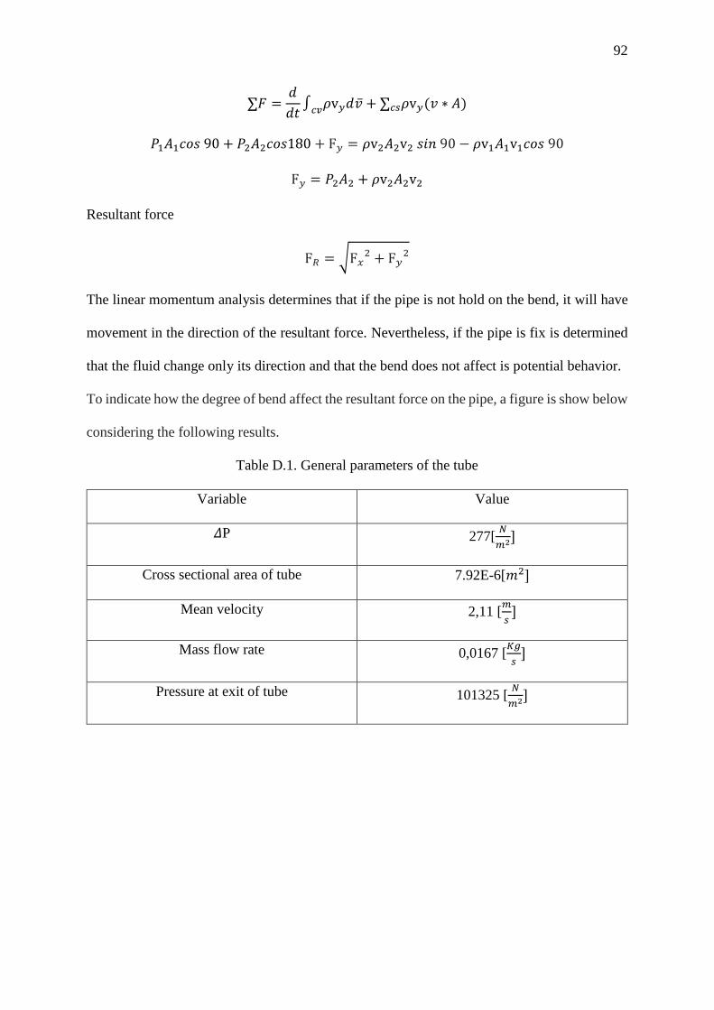
92
∑𝐹𝐹 =𝑑𝑑𝑑𝑑𝑑𝑑∫𝑐𝑐𝑐𝑐𝜌𝜌v𝑦𝑦𝑑𝑑�̅�𝑣 + ∑𝑐𝑐𝑠𝑠𝜌𝜌v𝑦𝑦(𝑣𝑣 ∗ 𝐴𝐴)
𝑃𝑃1𝐴𝐴1𝑐𝑐𝑙𝑙𝑁𝑁 90 + 𝑃𝑃2𝐴𝐴2𝑐𝑐𝑙𝑙𝑁𝑁180 + F𝑦𝑦 = 𝜌𝜌v2𝐴𝐴2v2 𝑁𝑁𝑠𝑠𝑛𝑛 90 − 𝜌𝜌v1𝐴𝐴1v1𝑐𝑐𝑙𝑙𝑁𝑁 90
F𝑦𝑦 = 𝑃𝑃2𝐴𝐴2 + 𝜌𝜌v2𝐴𝐴2v2
Resultant force
F𝑅𝑅 = �F𝑥𝑥2 + F𝑦𝑦2
The linear momentum analysis determines that if the pipe is not hold on the bend, it will have
movement in the direction of the resultant force. Nevertheless, if the pipe is fix is determined
that the fluid change only its direction and that the bend does not affect is potential behavior.
To indicate how the degree of bend affect the resultant force on the pipe, a figure is show below
considering the following results.
Table D.1. General parameters of the tube
Variable Value
𝛥𝛥P 277[ 𝑁𝑁𝑚𝑚2]
Cross sectional area of tube 7.92E-6[𝑚𝑚2]
Mean velocity 2,11 [𝑚𝑚𝑠𝑠
]
Mass flow rate 0,0167 [𝐾𝐾𝑔𝑔𝑠𝑠
]
Pressure at exit of tube 101325 [ 𝑁𝑁𝑚𝑚2]

93
Figure D3. Effect of DOB on the resultant force This indicate that the force in the x direction does not occupied a value importance in general,
due that the force that considers more is in the y direction. It is justified by the fact that as the
degree of bend increases, the x force decreases to approximate 0. The values obtained
demonstrate that the force impact on the bend is not critically and effects of it can be
disregarded.
Therefore, the conservation of momentum establishes that the fluid does not experience
changes in it, the same energy is conserved. However, from the friction losses analysis is
determine that the friction forces affected it, then, its kinetic energy change.
Pump calculation
𝑣𝑣12
2𝑔𝑔+𝑝𝑝1𝜌𝜌𝑔𝑔
+ 𝑑𝑑1 + 𝐻𝐻𝑃𝑃 =𝑣𝑣22
2𝑔𝑔+𝑝𝑝2𝜌𝜌𝑔𝑔
+ 𝑑𝑑2 + ℎ𝑙𝑙
ℎ𝑙𝑙 = ℎ𝑓𝑓 + ℎ𝑚𝑚 𝑣𝑣12
2𝑔𝑔+𝑝𝑝1𝜌𝜌𝑔𝑔
+ 𝑑𝑑1 + 𝐻𝐻𝑃𝑃 =𝑣𝑣22
2𝑔𝑔+𝑝𝑝2𝜌𝜌𝑔𝑔
+ 𝑑𝑑2 +𝑓𝑓𝐿𝐿𝑣𝑣2
𝐷𝐷2𝑔𝑔+𝑘𝑘𝑣𝑣2
2𝑔𝑔
𝐻𝐻𝑃𝑃 =𝑣𝑣2
2𝑔𝑔(𝑓𝑓𝐿𝐿𝐷𝐷
+ ∑𝐾𝐾𝑅𝑅 + 1)
𝐻𝐻𝑃𝑃 =𝑄𝑄2
2𝑔𝑔𝐴𝐴2(𝑓𝑓𝐿𝐿𝐷𝐷
+ ∑𝐾𝐾𝑅𝑅 + 1)
𝐻𝐻𝑃𝑃 =𝑄𝑄2
2𝑔𝑔𝐴𝐴2(𝑓𝑓𝐿𝐿𝐷𝐷
+ ∑𝐾𝐾𝑅𝑅 + 1)
0.00
0.10
0.20
0.30
0.40
0.50
0.60
0.70
0.80
0.90
0 20 40 60 80 100
Forc
e (N
)
DOB (°)
Fx
Fy
F
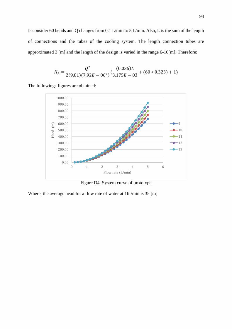
94
Is consider 60 bends and Q changes from 0.1 L/min to 5 L/min. Also, L is the sum of the length
of connections and the tubes of the cooling system. The length connection tubes are
approximated 3 [m] and the length of the design is varied in the range 6-10[m]. Therefore:
𝐻𝐻𝑃𝑃 =𝑄𝑄2
2(9.81)(7,92𝐸𝐸 − 062) ((0.035)𝐿𝐿
3.175𝐸𝐸 − 03+ (60 ∗ 0.323) + 1)
The followings figures are obtained:
Figure D4. System curve of prototype
Where, the average head for a flow rate of water at 1lit/min is 35 [m]
0.00
100.00
200.00
300.00
400.00
500.00
600.00
700.00
800.00
900.00
1000.00
0 1 2 3 4 5 6
Hea
d (m
)
Flow rate (L/min)
9
10
11
12
13