TREE:

A tree is a finite set of one or more nodes such that there is a specially designated node

called the Root, and zero or more non empty sub trees T1, T2....Tk, each of whose roots are

connected by a directed edge from Root R.

Example

ROOT: A node which doesn't have a parent. In the above tree. The Root is A.

NODE: Item of Information

LEAF: A node which doesn't have children is called leaf or Terminal node. Here B, K, L, G, H,

M, J are leafs.

SIBLINGS: Children of the same parents are said to be siblings, Here B, C, D, E , F, G are

siblings. Similarly I, J & K, L are siblings.

PATH: A path from node n, to nk is defined as a sequence of nodes n1, n2,n3....nk such that

ni is the parent of ni+1. There is exactly only one path from each node to root.

E.g.: Path from A to Q is A, E, J, Q. where A is the parent for E, E is the parent of J and J is the

parent of Q.

LENGTH: The length is defined as the number of edges on the path.

The length for the path A to Q is 3.

DEGREE: The number of subtrees of a node is called its degree.

Degree of A is 3

Degree of C is 0

Degree of D is 1

LEVEL: The level of a node is defined by initially letting the root be at level Zero, if a node is at

level L then its children are at level L + 1.

Level of A is 0.

Level of B, C, D, is 1.

Level of F, G, H, I, J is 2

Level of K, L, M is 3.

DEPTH: For any node n, the depth of n is the length of the unique path from root to n.

The depth of the root is zero.

HEIGHT: For any node n, the height of the node n is the length of the longest path from n to

the leaf.

The height of the leaf is zero

The height of the root A is 3.

The height of the node E is 2.

Note: The height of the tree is equal to the height of the root.

Depth of the tree is equal to the height of the tree.

ANCESTOR AND DESCENDANT: If there is a path from n1 to n2. n1 is an ancestor of n2, n2

is a descendant of n1.

IMPLEMENTATION OF TREES

Each node having a data, and pointer to each child of node. The number of children per

node can vary and is not known in advance, so it might be infeasible to make a children direct

links in the data datastructure, because there would be too much wasted space.

Here the arrow that point downward are FirstChild pointers. Arrow that go left to right are

NextSibling pointers. Null pointers are not drawn , there are too many.

BINARY TREE

Definition: - Binary Tree is a tree in which no node can have more than two children.

Maximum number of nodes at level i of a binary tree is 2i-1.

BINARY TREE NODE DECLARATIONS

Struct TreeNode {

int Element;

Struct TreeNode *Left ;

Struct TreeNode *Right;

};

Types of Binary Tress

1) Rooted Binary tree: - In which every node has atmost two children.

2) Full Binary Tree:-In which every node has zero or two children.

3) Perfect Binary Tree:- In which all the leaves are at same depth.

4) Complete Binary Tree:- In which all the leaves are at same depth n or n-1 for some n.

REPRESENTATION OF A BINARY TREE

There are two ways for representing binary tree, they are

* Linear Representation

* Linked Representation

Linear Representation

The elements are represented using arrays. For any element in position i, the left child is in

position 2i, the right child is in position (2i + 1), and the parent is in position (i/2)

1 2 3 4 5 6 7

E.g i=1, For node A, Left child at 2i=>2x1=2=>B, Right child at 2i+1=>(2x1)+1=3=>C

Linked Representation

The elements are represented using pointers. Each node in linked representation has three

fields, namely,

* Pointer to the left subtree

* Data field

A B C D E F G

* Pointer to the right subtree

In leaf nodes, both the pointer fields are assigned as NULL.

Tree Traversals

Traversing means visiting each node only once. Tree traversal is a method for visiting all the

nodes in the tree exactly once. There are three types of tree traversal techniques, namely

1. Inorder Traversal

2. Preorder Traversal

3. Postorder Traversal

Inorder Traversal

The inorder traversal of a binary tree is performed as

* Traverse the left subtree in inorder

* Visit the root

* Traverse the right subtree in inorder.

Example :

Inorder: A B C D E G H I J K

The inorder traversal of the binary tree for an arithmetic expression gives the expression in an

infix form.

RECURSIVE ROUTINE FOR INORDER TRAVERSAL

void Inorder (Tree T)

{

if (T ! = NULL)

{

Inorder (T->left);

printElement (T->Element);

Inorder (T->right);

}

}

Preorder Traversal

The preorder traversal of a binary tree is performed as follows,

* Visit the root

* Traverse the left subtree in preorder

* Traverse the right subtree in preorder.

Preorder: D C A B I G E H K J

The preorder traversal of the binary tree for the given expression gives in prefix form.

RECURSIVE ROUTINE FOR PREORDER TRAVERSAL

void Preorder (Tree T)

{

if (T ! = NULL)

{

printElement (T->Element);

Preorder (T->left);

Preorder (T->right);

}

Postorder Traversal

The postorder traversal of a binary tree is performed by the following steps.

* Traverse the left subtree in postorder.

* Traverse the right subtree in postorder.

* Visit the root.

Post order : B A C E H G J K I D

The postorder traversal of the binary tree for the given expression gives in postfix form.

RECURSIVE ROUTINE FOR POSTORDER TRAVERSAL

void Postorder (Tree T)

{

if (T ! = NULL)

{

Postorder (T->Left);

Postorder (T->Right);

PrintElement (T->Element);

}

EXAMPLE FOR TREE TRAVERSAL

Inorder : 5 10 15 20 25 30 40

Preorder : 20 10 5 15 30 25 40

Postorder : 5 15 10 25 40 30 20

EXPRESSION TREE

Expression Tree is a binary tree in which the leaf nodes are operands and the interior

nodes are operators. Like binary tree, expression tree can also be travesed by inorder, preorder

and postorder traversal.

Constructing an Expression Tree

Let us consider postfix expression given as an input for constructing an expression tree by

performing the following steps :

1. Read one symbol at a time from the postfix expression.

2. Check whether the symbol is an operand or operator.

(a) If the symbol is an operand, create a one - node tree and push a pointer on to the stack.

(b) If the symbol is an operator pop two pointers from the stack namely T1 and T2 and form a

new tree with root as the operator and T2 as a left child and T1 as a right child.

A pointer to this new tree is then pushed onto the stack.

Example: ab+cde+**

1) The first two symbols are operands, so create one-node tree & push pointers to them on

to a stack.

2) Next ‘+’ is read, so two pointers to trees are popped a new tree is formed and a pointer

is pushed on to a stack.

3) Next c,d,e are read and for each a one-node tree is created and a pointer to the

corresponding tree is pushed on to the stack

4) Now ‘+ is read, so two tree are merged.

5) Next ‘*’ is read, so pop two tree pointers and form a new tree with ‘*’ as root.

6) Next ‘*’ is read, two trees are merged, and a pointer to the final tree is left on the stack.

THE SEARCH TREE ADT: - BINARY SEARCH TREE

Definition: -

Binary search tree is a binary tree in which for every node X in the tree, the values of all

the keys in its left subtree are smaller than the key value in X, and the values of all the keys in

its right subtree are larger than the key value in X.

Note : * Every binary search tree is a binary tree.

* All binary trees need not be a binary search tree.

DECLARATION ROUTINE FOR BINARY SEARCH TREE

Struct TreeNode;

typedef struct TreeNode * SearchTree;

SearchTree Insert (int X, SearchTree T);

SearchTree Delete (int X, SearchTree T);

int Find (int X, SearchTree T);

int FindMin (Search Tree T);

int FindMax (SearchTree T);

SearchTree MakeEmpty (SearchTree T);

Struct TreeNode

{

int Element ;

SearchTree Left;

SearchTree Right;

};

Make Empty :-

This operation is mainly for initialization when the programmer prefer to initialize the first

element as a one - node tree.

ROUTINE TO MAKE AN EMPTY TREE :-

SearchTree MakeEmpty (SearchTree T)

{

if (T! = NULL)

{

MakeEmpty (T-> left);

MakeEmpty (T-> Right);

free (T);

}

return NULL ;

}

INSERT: -

To insert the element X into the tree,

* Check with the root node T

* If it is less than the root, Traverse the left subtree recursively until it reaches the T-> left

equals to NULL. Then X is placed in T-> left.

* If X is greater than the root. Traverse the right subtree recursively until it reaches the T->

right equals to NULL. Then x is placed in T->Right.

ROUTINE TO INSERT INTO A BINARY SEARCH TREE

SearchTree Insert (int X, searchTree T)

{

if (T = = NULL)

{

T = malloc (size of (Struct TreeNode));

if (T! = NULL) // First element is placed in the root.

{

T ->Element = X;

T-> left = NULL;

T -> Right = NULL;

}

}

else

if (X < T ->Element)

T ->left = Insert (X, T ->left);

else

if (X > T ->Element)

T ->Right = Insert (X, T ->Right);

// Else X is in the tree already.

return T;

}

Example : -

To insert 8, 4,1,6,5,7,10

* First element 8 is considered as Root.

*As 4< 8, Traverse towards left

*1<8, towards left & 1<4, towards left

*6<8, towards left & 6>4 then towards right.

*5<8, towards left and 5>4 towards right and 5<6 towards left

*7<8, towards left & 7>4, towards right and 7>6, towards right.

*finally 10>8 so move towards right.

FIND: -

* Check whether the root is NULL if so then return NULL.

* Otherwise, Check the value X with the root node value (i.e. T ->data)

(1) If X is equal to T ->data, return T.

(2) If X is less than T ->data, Traverse the left of T recursively.

(3) If X is greater than T ->data, traverse the right of T recursively.

ROUTINE FOR FIND OPERATION

Int Find (int X, SearchTree T)

{

If T = = NULL)

Return NULL ;

If (X < T->Element)

return Find (X, T->left);

else

If (X > T->Element)

return Find (X, T->Right);

else

return T; // returns the position of the search element.

}

Example : - To Find an element 7 (consider Previous example, X = 7)

7 is checked with the Root 7< 8, Go to the left child of 8

7 is checked with Root 4 7>4, Go to the right child of 4.

7 is checked with Root 6 7>6, Go to the right child of 6.

7 is checked with root 7 (Found)

FIND MIN

This operation returns the position of the smallest element in the tree. To perform

FindMin, start at the root and go left as long as there is a left child. The stopping point is the

smallest element.

RECURISVE ROUTINE FOR FINDMIN

int FindMin (SearchTree T)

{

if (T = = NULL);

return NULL ;

else if (T->left = = NULL)

return T;

else

return FindMin (T->left);

}

Example : -

Root T

(a) T! = NULL and T->left!=NULL, (b) T! = NULL and T->left!=NULL, Traverse left Traverse

left

(b) T! = NULL and T->left!=NULL, Traverse left Traverse left

(c) Since T left is Null, return T as a minimum element.

FINDMAX

FindMax routine return the position of largest elements in the tree. To perform a

FindMax, start at the root and go right as long as there is a right child. The stopping point is the

largest element.

RECURSIVE ROUTINE FOR FINDMAX

int FindMax (SearchTree T)

{

if (T = = NULL)

return NULL ;

else if (T->Right = = NULL)

return T;

else FindMax (T->Right);

}

Example :-

Root T

(a) T! = NULL and T->Right!=NULL, Traverse Right Traverse Right

(b) T! = NULL and T->Right!=NULL, Traverse Right Traverse Right

Max

(c) Since T Right is NULL, return T as a Maximum element

Delete :

Deletion operation is the complex operation in the Binary search tree. To delete an element,

consider the following three possibilities.

CASE 1: Node to be deleted is a leaf node (ie) No children.

CASE 2: Node with one child.

CASE 3: Node with two children.

CASE 1 Node with no children (Leaf node)

If the node is a leaf node, it can be deleted immediately.

CASE 2 : - Node with one child

If the node has one child, it can be deleted by adjusting its parent pointer that points to its child

node.

To Delete 5

To delete 5, the pointer currently pointing the node 5 is now made to to its child node 6

Before deletion After Deletion

Case 3 : Node with two children

It is difficult to delete a node which has two children. The general strategy is to replace the

data of the node to be deleted with its smallest data of the right subtree and recursively delete

that node.

Example 1 :

To Delete 5 :

* The minimum element at the right subtree is 7.

* Now the value 7 is replaced in the position of 5.

* Since the position of 7 is the leaf node delete immediately.

DELETION ROUTINE FOR BINARY SEARCH TREES

SearchTree Delete (int X, searchTree T) {

int Tmpcell ;

if (T = = NULL)

Error ("Element not found");

else

if (X < T->Element) // Traverse towards left

T->Left = Delete (X, T->Left);

else

if (X > T->Element) // Traverse towards right

T->Right = Delete (X, T->Right);

// Found Element to be deleted

else

// Two children

if (T->Left && T->Right)

{ // Replace with smallest data in right subtree

Tmpcell = FindMin (T->Right);

T->Element = Tmpcell->Element ;

T->Right = Delete (T->Element; T->Right);

}

else // one or zero children

{

Tmpcell = T;

if (T->Left = = NULL)

T = T->Right;

else if (T->Right = = NULL)

T = T->Left ;

free (TmpCell);

}

return T; }

THREADED BINARY TREE

During binary tree creation, for the leaf nodes there is no sub-tree further. So we just

setting the left and right field of leaf nodes as NULL, it is just wastage of the memory. So to

avoid NULL values in the node set the threads which are actually the links to predecessor and

successor nodes.

The Structure of the node is

struct thread

{

int data;

int lth,rth;

struct thread *left;

struct thread *right;

}

Inorder Threading Technique:

The basic idea in inorder threading is that the left thread should point to the

predecessor and the right thread points to the successor. Here assume head node as the

starting node and the root node of the tree is attached to left of head node.

Logic Explanation for Threaded binary tree:

In threaded binary tree, the NULL pointers are avoided. The left thread NULL pointer

should point to the predecessor and the right thread NULL pointer points to the successor.

There are two additional fields in each node named as lth and rth these fields indicate

whether left or right child is present. To set lth and rth field value as either 0 or 1. The value 0

indicates there is no left child. The value 1 indicates there is no right child.

Example: 10,8,6,12,9,11,14.

1) Initially create a dummy node which acts as a header of the tree.

lth Left data Right rth

0 NULL 1000 NULL 0

2) Take first value i.e. 10. The node with value 10 will be the root node and attach this

root node as left child of dummy node.

0 NULL 10 NULL 0

The NULL links of root’s left and right child will be pointed to dummy.

1 1000 NULL 0

0 10 0

3) Read ‘8’. The 8 will be compared with 10, 8<10, so attach 8 as left child of 10 and also

set root’s lth field to 1, indicating that the node 10 is having left child.

1 1000 NULL 0

1 10 0

4) Read 6, first compared to 10 (6<10), so go to left subtree then compared to 8 (6<8)

move to left sub tree. But lth field of node 8 is 0, indicating there is no left child to 8, so

attach 6 as left child to 8.

1 1000 NULL 0

1 10 0

0 8 0

1 8 0

0 6 0

5) Next ’12’. Compare to 10 (12>10).so attach 12 as right child of 10.

1 1000 NULL 0

1 10 0

6) Similarly attach 9, 11 and 14 as appropriate children.

AVL Tree : - (Adelson - Velskill and LANDIS)

An AVL tree is a binary search tree except that for every node in the tree, the height of the left and right subtrees can differ by atmost 1.

The height of the empty tree is defined to be - 1.

A balance factor is the height of the left subtree minus height of the right subtree. For an AVL tree all balance factor should be +1, 0, or -1. If the balance factor of any node in an AVL tree becomes less than -1 or greater than 1, the tree has to be balanced by making either single or double rotations.

An AVL tree causes imbalance, when any one of the following conditions occur.

1 8 0

0 6 0

Case 1: An insertion into the left subtree of the left child of node α

Case 2: An insertion into the right subtree of the left child of node α

Case 3: An insertion into the left subtree of the right child of node α

Case 4: An insertion into the right subtree of the right child of node α

These imbalances can be overcome by

1. Single Rotation

2. Double Rotation.

Single Rotation

Single Rotation is performed to fix case 1 and case 4.

Case 1. An insertion into the left subtree of the left child of K2. [LL ROTATION]

Single Rotation to fix Case 1.

General Representation

ROUTINE TO PERFORM SINGLE ROTATION WITH LEFT

SingleRotatewithLeft (Position K2)

{

Position K1;

K1 = K2 ->Left ;

K2 ->left = K1->Right ;

K1->Right = K2 ;

K2 ->Height = Max (Height (K2->Left), Height (K2-> Right)) + 1 ;

K1->Height = Max (Height (K1 ->left), K2->Height ) + 1;

return K1 ;

}

Example : Inserting the value `1' in the following AVL Tree makes AVL Tree imbalance

Before After

Single Rotation to fix Case 4 :-

Case 4 : - An insertion into the right subtree of the right child of K1. [RR ROTATION]

General Representation

ROUTINE TO PERFORM SINGLE ROTATION WITH RIGHT :-

Single Rotation With Right (Position K2)

{

Position K2 ;

K2 = K1->Right;

K1 ->Right = K2 ->Left ;

K2->Left = K1 ;

K1->Height = Max (Height (K1->Left), Height (K1-> Right)) +1 ;

K2 ->Height = Max (K1->Height, Height (K2 ->Right)) +1 ;

Return K2 ;

}

Example:

Double Rotation

Double Rotation is performed to fix case 2 and case 3.

Case 2 : An insertion into the right subtree of the left child. [RL ROTATION]

General Representation

ROUTINE TO PERFORM DOUBLE ROTATION WITH RIGHT:

Double Rotate with right (Position K1)

{ /* Rotation Between K2 & K3 */

K1 ->Right = Single Rotate with Left (K1 ->Right);

/* Rotation between K1 & K2 */

Return Single Rotate With Right (K1);

}

Example:

Case 3 : An insertion into the left subtree of the right child. [LR ROTATION]

General Representation

ROUTINE TO PERFORM DOUBLE ROTATION WITH LEFT:

Double Rotate with left (Position K3)

{ /* Rotation Between K1 & K2 */

K3 ->Left = Single Rotate with Right (K3 ->Left);

/* Rotation Between K3 & K2 */

Return Single Rotate With Left (K3);

}

Example:

ROUTINE TO INSERT IN AN AVL TREE : -

AVLTree Insert (AVL tree T, int X)

{

if (T = = NULL)

{

T = malloc (size of (Struct AVLnode));

if (T = = NULL)

Error ("out of space");

else

{

T->data =X;

T ->Height = 0;

T ->Left = NULL;

T ->Right = NULL;

}

}

else

if (X < T->data)

{

T ->left = Insert (T->left, X);

if (Height (T -> left) - Height (T->Right) = = 2)

if (X < T->left->data)

T = Single Rotate With left (T);

else

T = Double Rotate is the left (T);

}

else

if (X > T->data)

{

T ->Right = Insert (T->Right, X);

if (Height (T->Right) - Height (T->left) = = 2)

if(X > T->Right->Element)

T = Single Rotate with Right (T);

else

T = Double Rotate with Right (T);

}

T->Height = Max (Height (T->left), Height (T->Right))+1;

return T;

}

Example:

Example: 3, 6, 5, 1, 2, 4

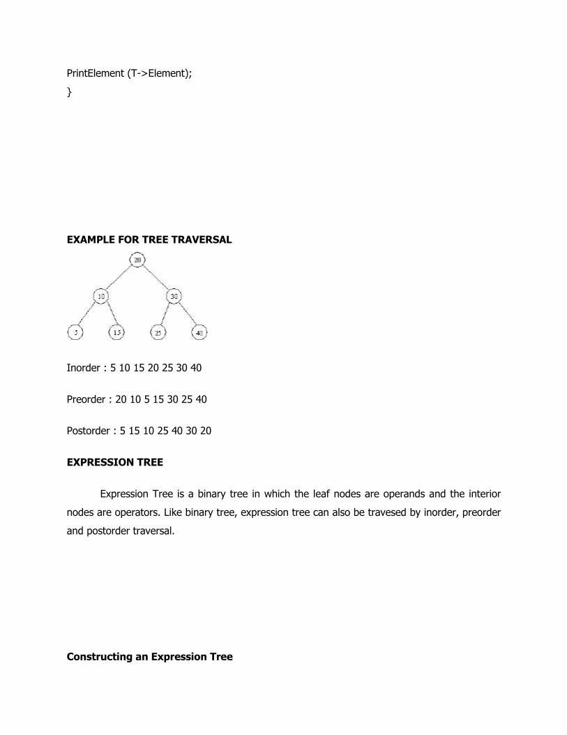
SPLAY TREES

1) Splay tress are variation of binary search tree.

2) The basic idea is not to spend too much time on balancing.

Key Idea:

The frequently accessed nodes are rotated as close as possible to the root. Whenever an

object is accessed, it becomes the new root. It should be done without adversely affecting

other nodes.

SPLAYING

1) If the accessed node is already is already in the root, nothing to do.

2) If the accessed node X has root as its parent then rotate X with its parent.

3) Otherwise ( X has both parent & Grant parent) there are four possible cases:-

a) X is left - right of GP

b) X is right – left of GP

c) X is left – left of P

d) X is right – right of P

Zig – Zag

Zig – Zig

1) K2 is the root that has no parent

2) X and P has either both left or both right children. Transforms the tree on the left to

right.

Zig – Zag (Double Rotation)

Zig – Zig (Single Rotation)

EXAMPLE: Make K1 as TOP

1) The first splay step is at k1, and is clearly a zig-zag, so we perform a standard AVL

double rotation using k1, k2, and k3. The resulting tree follows.

2) The next splay step at k1 is a zig-zig, so we do the zig-zig rotation with k1, k4, and k5, obtaining the final tree.

GRAPH

A graph G = (V, E) consists of a set of vertices, V and set of edges E. Vertices are referred to as nodes and the arc between the nodes are referred to as Edges. Each edge is a pair (v, w) where u, w V. (i.e.) v = V1, w = V2... Here V1, V2, V3, V4 are the vertices and (V1, V2), (V2, V3), (V3, V4), (V4, V1), (V2, V4), (V1, V3) are edges. BASIC TERMINOLOGIES Directed Graph (or) Digraph

Directed graph is a graph which consists of directed edges, where each edge in E is unidirectional. It is also referred as Digraph. If (v, w) is a directed edge then (v, w) # (w, v) (V1, V2) # (V2, V1) Undirected Graph

An undirected graph is a graph, which consists of undirected edges. If (v, w) is an undirected edge then (v,w) = (w, v) (V1, V2) = (V2, V1)

Weighted Graph

A graph is said to be weighted graph if every edge in the graph is assigned a weight or value. It can be directed or undirected grap Complete Graph

A complete graph is a graph in which there is an edge between every pair of vertices. A complete graph with n vertices will have n (n - 1)/2 edges.

Degree

The number of edges incident on a vertex determines its degree. The degree of the vertex V is written as degree (V).

The indegree of the vertex V, is the number of edges entering into the vertex V.

Similarly the out degree of the vertex V is the number of edges exiting from that vertex V.

Number of vertics is 4 Number of edges is 6 (i.e) there is a path from every vertex to every other vertex. A complete digraph is a strongly connected graph. Strongly Connected Graph

If there is a path from every vertex to every other vertex in a directed graph then it is

said to be strongly connected graph. Otherwise, it is said to be weakly connected graph.

Strongly Connected Graph Weakly Connected Graph Path A path in a graph is a sequence of vertices ω1, ω2, …. ωn such that ωi, ωi+1 Є E for 1 ≤ i ≤ N. The path from above diagram V1 to V3 is V1, V2 and V3. Length

The length of the path is the number of edges on the path, which is equal to N-1, where N represents the number of vertices. The length of the above path V1 to V3 is 2. (i.e) (V1, V2), (V2, V3). If there is a path from a vertex to itself, with no edges, then the path length is 0. Loop

If the graph contains an edge (v, v) from a vertex to itself, then the path is referred to as a loop. Simple Path

A simple path is a path such that all vertices on the path, except possibly the first and the last are distinct.

A simple cycle is the simple path of length atleast one that begins and ends at the same vertex. Cycle

A cycle in a graph is a path in which first and last vertex are the same. A graph which has cycle is referred to as cyclic graph Degree

The number of edges incident on a vertex determines its degree. The degree of the vertex V is written as degree (V). The indegree of the vertex V, is the number of edges entering into the vertex V. Similarly the out degree of the vertex V is the number of edges exiting from that vertex V.

Indegree (V1) = 2 Outdegree (V2) = 1 Acyclic Graph

A directed graph which has no cycles is referred to as acyclic graph. It is abbreviated as DAG. DAG - Directed Acyclic Graph. REPRESENTATION OF GRAPH Graph can be represented by Adjacency Matrix and Adjacency list. Adjacency Matrix

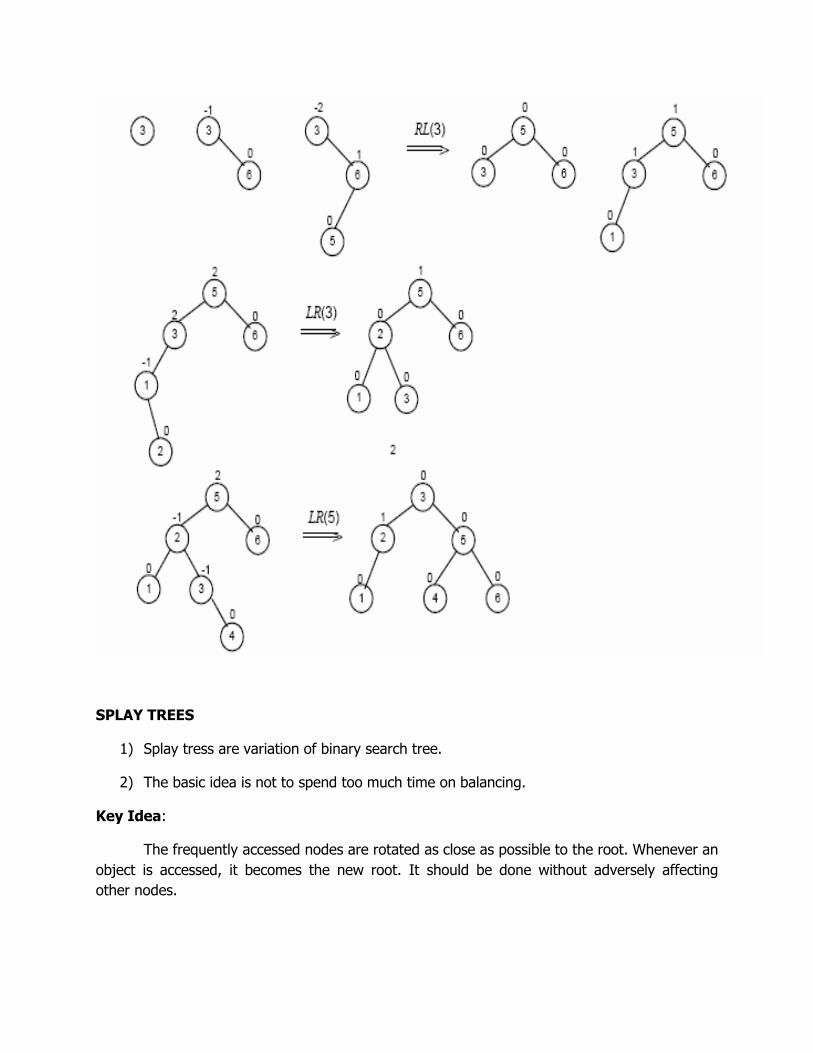
One simple way to represents a graph is Adjacency Matrix. The adjacency Matrix A for a graph G = (V, E) with n vertices is an n x n matrix, such that Aij = 1, if there is an edge Vi to Vj

Aij = 0, if there is no edge. Adjacency Matrix For Directed Graph

0 1 1 0

0 0 0 1

0 1 0 0

0 0 1 0

Example V1,2 = 1 Since there is an edge V1 to V2 Similarly V1,3 = 1, there is an edge V1 to V3 V1,1 & V1,4 = 0, there is no edge. Adjacency Matrix for Undirected Graph

Adjacency Matrix for Weighted Graph To solve some graph problems, Adjacency matrix can be constructed as Aij = Cij, if there exists an edge from Vi to Vj Aij = 0, if there is no edge & i = j If there is no arc from i to j, Assume C[i, j] = ∞ where i ≠ j.

Adjacency Matrix for Undirected Graph

Advantage * Simple to implement. Disadvantage * Takes O(n2) space to represents the graph * It takes O(n2) time to solve the most of the problems. Adjacency List Representation

In this representation, we store a graph as a linked structure. We store all vertices in a list and then for each vertex, we have a linked list of its adjacency vertices

0 1 1 0

1 0 1 1

1 1 0 1

0 1 1 0

0 3 9 ∞

∞ 0 ∞ 7

∞ 1 0 ∞

∞ 1 8 0

Disadvantage

* It takes 0(n) time to determine whether there is an arc from vertex i to vertex j. Since there can be 0(n) vertices on the adjacency list for vertex i.

Topological Sort

A topological sort is a linear ordering of vertices in a directed acyclic graph such that if there is a path from Vi to Vj, then Vj appears after Vi in the linear ordering.

Topological ordering is not possible. If the graph has a cycle, since for two vertices v and w on the cycle, v precedes w and w precedes v. To implement the topological sort, perform the following steps.

Step 1: - Find the indegree for every vertex. Step 2: - Place the vertices whose indegree is `0' on the empty queue. Step 3: - Dequeue the vertex V and decrement the indegree's of all its adjacent vertices. Step 4: - Enqueue the vertex on the queue, if its indegree falls to zero. Step 5: - Repeat from step 3 until the queue becomes empty. Step 6: - The topological ordering is the order in which the vertices dequeued. Routine to perform Topological Sort /* Assume that the graph is read into an adjacency matrix and that the indegrees are computed for every vertices and placed in an array (i.e. Indegree [ ] ) */ void Topsort (Graph G) { Queue Q ; int counter = 0; Vertex V, W ; Q = CreateQueue (NumVertex); Makeempty (Q); for each vertex V if (indegree [V] = = 0) Enqueue (V, Q); while (! IsEmpty (Q)) { V = Dequeue (Q); TopNum [V] = + + counter; for each W adjacent to V if (--Indegree [W] = = 0) Enqueue (W, Q); } if (counter ! = NumVertex) Error (" Graph has a cycle"); DisposeQueue (Q); /* Free the Memory */ } Note : Enqueue (V, Q) implies to insert a vertex V into the queue Q. Dequeue (Q) implies to delete a vertex from the queue Q. TopNum [V] indicates an array to place the topological numbering. Example 1:

0 1 1 0

0 0 1 1

0 0 0 1

0 0 0 0

Step 1 Number of 1's present in each column of adjacency matrix represents the indegree of the corresponding vertex. Indegree [a] = 0 Indegree [b] = 1 Indegree [c] = 2 Indegree [d] = 2 Step 2 Enqueue the vertex, whose indegree is `0' Vertex `a' is 0, so place it on the queue. Step 3 Dequeue the vertex `a' from the queue and decrement the indegree's of its adjacent vertex `b' & `c' Hence, Indegree [b] = 0 & Indegree [c] = 1 Now, Enqueue the vertex `b' as its indegree becomes zero. Step 4 Dequeue the vertex `b' from Q and decrement the indegree's of its adjacent vertex `c' and `d'. Hence, Indegree [c] = 0 & Indegree [d] = 1 Now, Enqueue the vertex `c' as its indegree falls to zero. Step 5 Dequeue the vertex `c' from Q and decrement the indegree's of its adjacent vertex `d'. Hence, Indegree [d] = 0 Now, Enqueue the vertex `d' as its indegree falls to zero. Step 6 Dequeue the vertex `d'. Step 7 As the queue becomes empty, topological ordering is performed, which is nothing but, the order in which the vertices are dequeued.

VERTEX 1 2 3 4

a 0 0 0 0

b 1 0 0 0

c 2 1 0 0

d 2 2 1 0

ENQUEUE a b c d

DEQUEUE a b c d

Example 2

Adjacency matrix:-

V1 V2 V3 V4 V5 V6 V7

V1 0 1 1 1 0 0 0

V2 0 0 0 1 1 0 0

V3 0 0 0 0 0 1 0

V4 0 0 1 0 0 1 1

V5 0 0 0 1 0 0 1

V6 0 0 0 0 0 0 0

V7 0 0 0 0 0 1 0

INDEGREE 0 1 2 3 1 3 2

Indegree [v1] = 0 Indegree [v2] = 1 Indegree [v3] = 2 Indegree [v4] = 3

Indegree [v5] = 1 Indegree [v6] = 3 Indegree [v7] = 2

VERTEX 1 2 3 4 5 6 7

V1 0 1 1 1 0 0 0

V2 0 0 0 1 1 0 0

V3 0 0 0 0 0 1 0

V4 0 0 1 0 0 1 1

V5 0 0 0 1 0 0 1

V6 0 0 0 0 0 0 0

V7 0 0 0 0 0 1 0

ENQUEUE V1 V2 V5 V4 V3,V7 V6

DEQUEUE V1 V2 V5 V4 V3 V7 V6

Therefore, the topological order is V1, V2, V3, V4, V5, V7 and V6.

Shortest Path Algorithm The Shortest path algorithm determines the minimum cost of the path from source to

every other vertex. The cost of the path V1, V2, --VN is . This is referred as weighted path length.

The unweighted path length is merely the number of the edges on the path, namely N - 1. Two types of shortest path problems, exist namely, 1. The single source shortest path problem

2. The all pairs shortest path problem The single source shortest path algorithm finds the minimum cost from single source vertex to all other vertices. Dijkstra's algorithm is used to solve this problem which follows the greedy technique. All pairs shortest path problem finds the shortest distance from each vertex to all other vertices. To solve this problem dynamic programming technique known as floyd's algorithm is used. These algorithms are applicable to both directed and undirected weighted graphs provided that they do not contain a cycle of negative length. Single Source Shortest Path

Given an input graph G = (V, E) and a distinguished vertex S, find the shortest path from S to every other vertex in G. This problem could be applied to both weighted and unweighted graph. Unweighted Shortest Path

In unweighted shortest path all the edges are assigned a weight of "1" for each vertex, the following three pieces of information is maintained. Algorithm for unweighted graph Known Specifies whether the vertex is processed or not. It is set to `1' after it is processed, otherwise `0'. Initially all vertices are marked unknown. (i.e) `0'. dv Specifies the distance from the source `s', initially all vertices are unreachable except for s, whose path length is `0'. Pv Specifies the bookkeeping variable which will allow us to print. The actual path. (i.e) The vertex which makes the changes in dv. To implement the unweighted shortest path, perform the following steps : Step 1: - Assign the source node as `s' and Enqueue `s'. Step 2: - Dequeue the vertex `s' from queue and assign the value of that vertex to be known and then find its adjacency vertices. Step 3:- If the distance of the adjacent vertices is equal to infinity then change the distance of that vertex as the distance of its source vertex increment by `1' and Enqueue the vertex. Step 4:- Repeat from step 2, until the queue becomes empty. ROUTINE FOR UNWEIGHTED SHORTEST PATH

void Unweighted (Table T) { Queue Q; Vertex V, W ; Q = CreateQueue (NumVertex); MakeEmpty (Q); /* Enqueue the start vertex s */ Enqueue (s, Q); while (! IsEmpty (Q)) { V = Dequeue (Q); V = Dequeue (Q); T[V]. Known = True; /* Not needed anymore*/ for each W adjacent to V if (T[W]. Dist = = INFINITY) { T[W] . Dist = T[V] . Dist + 1 ; T[W] . path = V; Enqueue (W, Q); } } DisposeQueue (Q) ; /* Free the memory */ }

Example

Source vertex ‘a’ is initially assigned a path length ‘0’.

After finding all vertices whose path length from ‘a’ is 1.

V Known dv pv

a 0 0 0

b 0 ∞ 0

c 0 ∞ 0

d 0 ∞ 0

Queue a

After finding all vertices whose path length from ‘a’ is 2.

Shortest path from source a vertex ‘a’ to other vertices are

a→ b is 1 a → c is 1

a → d is 2

Example 2

V3 is taken as a source node and its path length is initialized to ‘0’.

V Known dv pv

a 1 0 0

b 0 1 a

c 0 1 a

d 0 ∞ 0

Queue b, c Dequeue ‘a’

V Known dv pv

a 1 0 0

b 1 1 a

c 0 1 a

d 0 2 b

Queue c, d Dequeue ‘b’

V Known dv pv

a 1 0 0

b 1 1 a

c 1 1 a

d 0 2 b

Queue d Dequeue ‘c’

V Known dv pv

a 1 0 0

b 1 1 a

c 1 1 a

d 1 2 b

Queue empty Dequeue ‘d’

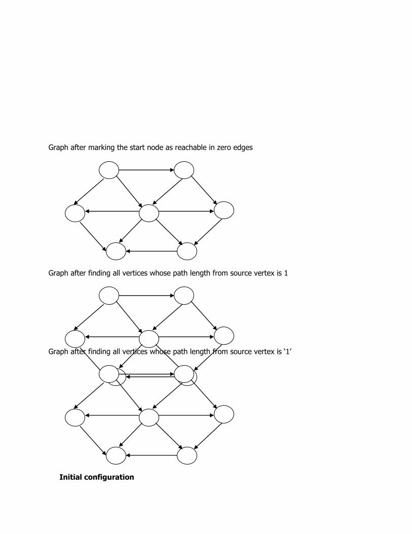
Graph after marking the start node as reachable in zero edges

Graph after finding all vertices whose path length from source vertex is 1

Graph after finding all vertices whose path length from source vertex is ‘1’

Initial configuration

V Known dv pv

V1 0 ∞ 0

V2 0 ∞ 0

V3 0 0 0

V4 0 ∞ 0

V5 0 ∞ 0

V6 0 ∞ 0

V7 0 ∞ 0

In general when the vertex `V' is dequeued and the distance of its adjacency vertex `w' is infinitive then distance and path of `w' is calculated as follows T [W]. Dist = T[V]. Dist + 1 T[W]. path = V When V3 is dequeued, known is set to 1 for that vertex the distance of its adjacent vertices V1 and V6 are updated if INFINITY. Path length of V1 is calculated as

T [V1]. Dist = T [V3]. Dist + 1 = 0 + 1 = 1 and its actual path is also calculated as T [V1] .path = V3 lllly T [V6]. Dist = T[V3]. Dist + 1 = 1 T [V6]. Path = V3 Similarly, when the other vertices are dequeued, the table is updated.

Initial state V3 Dequeued V1 Dequeued

V Known dv pv Known dv pv Known dv pv

V1 0 ∞ 0 0 1 V3 1 1 V3

V2 0 ∞ 0 0 ∞ 0 0 2 V1

V3 0 0 0 1 0 0 1 0 0

V4 0 ∞ 0 0 ∞ 0 0 2 V1

V5 0 ∞ 0 0 ∞ 0 0 ∞ 0

V6 0 ∞ 0 0 1 V3 0 1 V3

V7 0 ∞ 0 0 ∞ 0 0 ∞ 0

Q: V3 V1, V6 V6, V2, V4

V6 Dequeued V2 Dequeued V4 Dequeued

V Known dv pv Known dv pv Known dv pv

V1 1 1 V3 1 1 V3 1 1 V3

V2 0 2 V1 1 2 V1 1 2 V1

V3 1 0 0 1 0 0 1 0 0

V4 0 2 V1 0 2 V1 1 2 V1

V5 0 ∞ 0 0 3 V2 0 3 V2

V6 1 1 V3 1 1 V3 1 1 V3

V7 0 ∞ 0 0 ∞ 0 0 3 V4

Q: V2, V4 V4, V5 V5, V7

V5 Dequeued V7 Dequeued

V Known dv pv Known dv pv

V1 1 1 V3 1 1 V3

V2 1 2 V1 1 2 V1

V3 1 0 0 1 0 0

V4 1 2 V1 1 2 V1

V5 1 3 V2 1 3 V2

V6 1 1 V3 1 1 V3

V7 0 3 V4 1 3 V4

Q: V7 EMPTY

Data changes during the unweighted shortest path algorithm. The shortest distance from the source vertex V3 to all other vertex is listed below: V3 → V1 is 1 V3 → V2 is 2

V3 → V4 is 2 V3 → V5 is 3

V3 → V6 is 1 V3 → V7 is 3

Dijkstra's Algorithm

The general method to solve the single source shortest path problem is known as Dijkstra's algorithm. This is applied to the weighted graph G.

Dijkstra's algorithm is the prime example of Greedy technique, which generally solves a problem in stages by doing what appears to be the best thing at each stage. This algorithm proceeds in stages, just like the unweighted shortest path algorithm. At each stage, it selects a vertex v, which has the smallest dv among all the unknown vertices, and declares that as the shortest path from S to V and mark it to be known. We should set dw = dv + Cvw, if the new value for dw would be an improvement.

ROUTINE FOR ALGORITHM Void Dijkstra (Graph G, Table T) { int i ; vertex V, W; Read Graph (G, T) /* Read graph from adjacency list */ /* Table Initialization */ for (i = 0; i < Numvertex; i++) { T [i]. known = False; T [i]. Dist = Infinity; T [i]. path = NotA vertex; } T [start]. dist = 0; for ( ; ;) { V = Smallest unknown distance vertex; if (V = = Not A vertex) break ; T[V]. known = True; for each W adjacent to V if ( ! T[W]. known) { T [W]. Dist = Min [T[W]. Dist, T[V]. Dist + CVW] T[W]. path = V; } } }

Example 1:

Vertex `a' is chooses as source and is declared as known vertex. Then the adjacent vertices of `a' is found and their distances are updated as follows: T [b]. Dist = Min [T[b]. Dist, T[a]. Dist + Ca,b] = Min [∞, 0 + 2] = 2 T [d]. Dist = Min [T[d]. Dist, T[a]. Dist + Ca,d] = Min [∞, 0 + 1] = 1

V Known dv pv

a 0 0 0

b 0 ∞ 0

c 0 ∞ 0

d 0 ∞ 0

V Known dv pv

Now, select the vertex with minimum distance, which is not known and mark that vertex as visited. Here `d' is the next minimum distance vertex. The adjacent vertext to `d' is `c', therefore, the distance of c is updated a follows, T[c]. Dist = Min [T[c]. Dist, T[d]. Dist + Cd, c] = Min [, 1 + 1] = 2

The next minimum vertex is b and marks it as visited. Since the adjacent vertex d is already visited, select the next minimum vertex `c' and mark it as visited.

Example 2

a 1 0 0

b 0 2 a

c 0 ∞ 0

d 0 1 a

V Known dv pv

a 1 0 0

b 0 2 a

c 0 2 d

d 1 1 a

V Known dv pv

a 1 0 0

b 1 2 a

c 0 2 d

d 1 1 a

V Known dv pv

a 1 0 0

b 1 2 a

c 1 2 d

d 1 1 a

V Known dv pv

V1 0 0 0

V1 is taken as source vertex, and is marked known. Then the dv and Pv of its adjacent vertices are updated.

V2 0 ∞ 0

V3 0 ∞ 0

V4 0 ∞ 0

V5 0 ∞ 0

V6 0 ∞ 0

V7 0 ∞ 0

V Known dv pv

V1 1 0 0

V2 0 2 V1

V3 0 ∞ 0

V4 0 1 V1

V5 0 ∞ 0

V6 0 ∞ 0

V7 0 ∞ 0

V Known dv pv

V1 1 0 0

V2 0 2 V1

V3 0 3 V4

V4 1 1 V1

V5 0 3 V4

V6 0 9 V4

V7 0 5 V4

V Known dv pv

V1 1 0 0

V2 1 2 V1

V3 0 3 V4

V4 1 1 V1

V5 0 3 V4

V6 0 9 V4

V7 0 5 V4

V Known dv pv

V1 1 0 0

V2 1 2 V1

V3 0 3 V4

V4 1 1 V1

V5 1 3 V4

V6 0 9 V4

V7 0 5 V4

V Known dv pv

V1 1 0 0

V2 1 2 V1

V3 1 3 V4

V4 1 1 V1

V5 1 3 V4

V6 0 8 V3

V7 0 5 V4

The shortest distance from the source vertex V1 to all other vertex is listed below : V1 →V2 is 2 V1 →V3 is 3

V1 →V4 is 1 V1 →V5 is 3 V1 →V6 is 6 V1 →V7 is 5

MINIMUM SPANNING TREE

A spanning tree of a connected graph is its connected a cyclic subgraph that contains all the vertices of the graph.

A minimum spanning tree of a weighted connected graph G is its spanning tree of the smallest weight, where the weight of a tree is defined as the sum of the weights on all its edges.

The total number of edges in Minimum Spanning Tree (MST) is |V|-1 where V is the number of vertices. A minimum spanning tree exists if and only if G is connected. For any spanning Tree T, if an edge e that is not in T is added, a cycle is created. The removal of any edge on the cycle reinstates the spanning tree property.

V Known dv pv

V1 1 0 0

V2 1 2 V1

V3 1 3 V4

V4 1 1 V1

V5 1 3 V4

V6 0 6 V7

V7 1 5 V4

V Known dv pv

V1 1 0 0

V2 1 2 V1

V3 1 3 V4

V4 1 1 V1

V5 1 3 V4

V6 1 6 V7

V7 1 5 V4

Example

Spanning tree for the above graph

cost = 7 cost = 8

Cost=9 cost =8 cost = 5

Minimum spanning tree

Prim's Algorithm

Prim's algorithm is one of the way to compute a minimum spanning tree which uses a greedy technique. This algorithm begins with a set U initialised to {1}. It this grows a spanning tree, one edge at a time. At each step, it finds a shortest edge (u,v) such that the cost of (u, v) is the smallest among all edges, where u is in Minimum Spanning Tree and V is not in Minimum Spanning Tree.

Example:-

Here, `a' is taken as source vertex and marked as visited. Then the distance of its adjacent vertex is updated as follows: T[b].dist = Min [T[b].Dist, Ca,b] = Min (∞, 2) = 2 T[b].dist = Min [T[d].Dist, Ca,b] = Min (∞, 1) = 1 T[c].dist = Min [T[c].Dist, Ca,b] = Min (∞, 3) = 3

Next, vertex `d' with minimum distance is marked as visited and the distance of its unknown adjacent vertex is updated.

T[b].Dist = Min [T[b].Dist, Cd,b] = Min (2, 2)

= 2

V Known dv pv

a 0 0 0

b 0 ∞ 0

c 0 ∞ 0

d 0 ∞ 0

V Known dv pv

a 1 0 0

b 0 2 a

c 0 3 a

d 0 1 a

T[c].dist = Min [T[c].Dist, Cd,c] = Min (3,1)

Next, the vertex with minimum cost `c' is marked as visited and the distance of its unknown adjacent vertex is updated.

Since, there is no unknown vertex adjacent to `c', there is no updation in the distance. Finally, the vertex `b' which is not visited is marked.

V Known dv pv

a 1 0 0

b 0 2 a

c 0 1 d

d 1 1 a

V Known dv pv

a 1 0 0

b 0 2 a

c 1 1 d

d 1 1 a

V Known dv pv

a 1 0 0

b 1 2 a

c 1 1 d

d 1 1 a

The minimum cost of this spanning

Tree is 4 [i.e Ca, b + Ca,d + Cc, d]

Example 2

Consider V1 as source vertex and proceed from there.

Vertex V1 is marked as visited and then the distance of its adjacent vertices are updated as follows.

T[V2].dist = Min [T[V2].dist, Cv1, v2] = Min [∞, 2]

V Known dv pv

V1 0 0 0

V2 0 ∞ 0

V3 0 ∞ 0

V4 0 ∞ 0

V5 0 ∞ 0

V6 0 ∞ 0

V7 0 ∞ 0

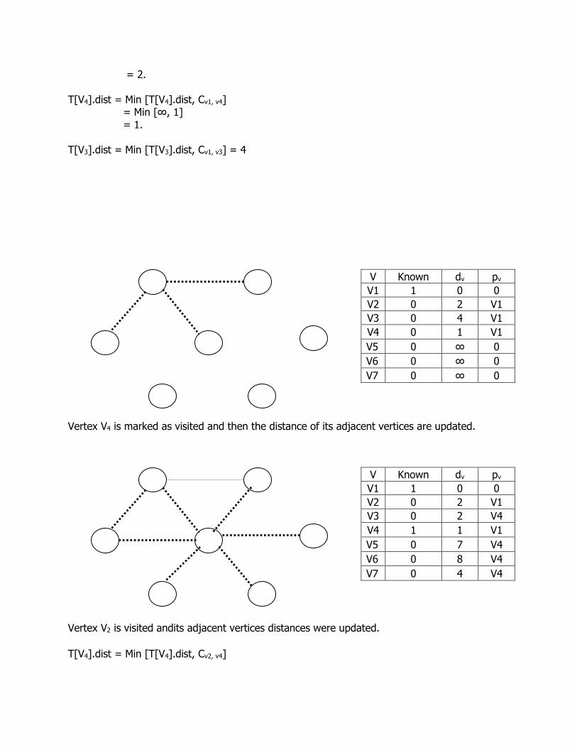
= 2. T[V4].dist = Min [T[V4].dist, Cv1, v4] = Min [∞, 1] = 1. T[V3].dist = Min [T[V3].dist, Cv1, v3] = 4

Vertex V4 is marked as visited and then the distance of its adjacent vertices are updated.

Vertex V2 is visited andits adjacent vertices distances were updated.

T[V4].dist = Min [T[V4].dist, Cv2, v4]

V Known dv pv

V1 1 0 0

V2 0 2 V1

V3 0 4 V1

V4 0 1 V1

V5 0 ∞ 0

V6 0 ∞ 0

V7 0 ∞ 0

V Known dv pv

V1 1 0 0

V2 0 2 V1

V3 0 2 V4

V4 1 1 V1

V5 0 7 V4

V6 0 8 V4

V7 0 4 V4

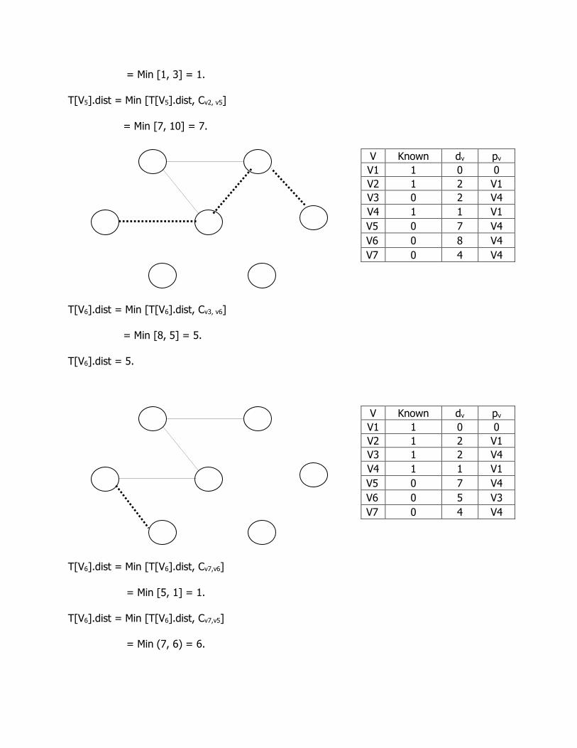
= Min [1, 3] = 1.

T[V5].dist = Min [T[V5].dist, Cv2, v5]

= Min [7, 10] = 7.

T[V6].dist = Min [T[V6].dist, Cv3, v6]

= Min [8, 5] = 5.

T[V6].dist = 5.

T[V6].dist = Min [T[V6].dist, Cv7,v6]

= Min [5, 1] = 1.

T[V6].dist = Min [T[V6].dist, Cv7,v5]

= Min (7, 6) = 6.

V Known dv pv

V1 1 0 0

V2 1 2 V1

V3 0 2 V4

V4 1 1 V1

V5 0 7 V4

V6 0 8 V4

V7 0 4 V4

V Known dv pv

V1 1 0 0

V2 1 2 V1

V3 1 2 V4

V4 1 1 V1

V5 0 7 V4

V6 0 5 V3

V7 0 4 V4

The minimum cost of this spanning tree is 16.

V Known dv pv

V1 1 0 0

V2 1 2 V1

V3 1 2 V4

V4 1 1 V1

V5 0 6 V7

V6 0 1 V7

V7 1 4 V4

V Known dv pv

V1 1 0 0

V2 1 2 V1

V3 1 2 V4

V4 1 1 V1

V5 0 6 V7

V6 1 1 V7

V7 1 4 V4

V Known dv pv

V1 1 0 0

V2 1 2 V1

V3 1 2 V4

V4 1 1 V1

V5 1 6 V7

V6 1 1 V7

V7 1 4 V4

Kruskal’s algorithm

Kruskal’s algorithm uses a greedy technique to compute a minimum spanning tree. This algorithm selects the edges in the order of smallest weight and accept an edge if it does not cause a cycle. The algorithm terminates if enough edges are accepted.

In general Kruskal’s algorithm maintains a forest – a collection of trees. Initially, there are |V| single node trees. Adding an edge merges two trees into one. When the algorithm terminates, there is only one tree, which is called as minimum spanning tree.

Example 1

Step 1: Initially each vertex is in its own set.

Step 2: Now, select the edge with minimum weight

Edge (a, d) is added to the minimum spanning tree.

Step 3: Select the next edge, with minimum weight and check whether it forms a cycle. If it forms a cycle, then that edge is rejected, else add the edge to the minimum spanning tree.

Step 4: Repeat step 3 until all vertices are included in the minimum spanning tree.

The minimum cost of this spanning tree is 4. [i.e., cost(a, d) + cost (c, d) + cost (a, b)]

Edge Weight Action

(a, d) 1 Accepted

(c, d) 1 Accepted

(a, d) 2 Accepted

Since all vertices are added the algorithm terminates.

Example 2

Step 1:

Step 2:

Step 3

Step 4:

Step 5:

Step 6

Edge Weight Action

(V1,V4) 1 Accepted

(V6,V7) 1 Accepted

(V1,V2) 2 Accepted

(V3,V4) 2 Accepted

(V2,V4) 3 Rejected

(V1,V3) 4 Rejected

(V4,V7) 4 Accepted

(V3,V6) 5 Rejected

(V5,V7) 6 Accepted

GRAPH TRAVERSAL

A graph traversal is a systematic way of visiting the nodes in a specific order. There are two types namely,

1) Breadth first traversal 2) Depth first traversal

Breadth first traversal

Breadth first search (BFS) of a graph G starts from an unvisited vertex u. then all the unvisited vertices vi adjacent to u are visited and then all unvisited vertices wj adjacent to vi are visited and so on. The traversal terminates when there are no more nodes tp visit. BFS uses a queue data structure to keep track of the order of nodes whose adjacent nodes are to be visited.

Steps to be implemented in BFS

Step 1: choose any node in the graph, designate it as search node and mark it as visited.

Step 2: using the adjacency matrix of the graph, find all the unvisited adjacent node to the search node and enqueue them into the queue Q.

Step 3: Then the node is dequeued from the queue. Mark that node as visited and designate it as new search node.

Step 4: Repeat step 2 and 3 using the new search node.

Step 5: This process continues until the queue Q which keeps track of the adjacent nodes is empty.

Example:

Adjacency matrix

A B C D

A 0 1 1 0

B 1 0 1 1

C 1 1 0 1

D 0 1 1 0

Implementation

1. Let ‘A’ be the source vertex. Mark it to as visited. 2. Find the adjacent unvisited vertices of ‘A’ and enqueue then into the queue. Here B

and C are adjacent nodes of A 3. Then vertex ‘B’ is dequeued and its adjacent vertices C and D are taken from the

adjacency matrix for enqueuing. Since vertex C is already in the queue, vertex D alone is enqueued. Here B is dequeued, D is enqueued.

4. Then vertex ‘C’ is dequeued and its adjacent vertices A,B and D are found. Since vertices A and B are already visited and vertex D is also in the queue, no enqueue operation takes place. Here C is dequeued.

5. Then vertex ‘D’ is dequeued. This process terminates as all the vertices are visited and the queue is empty.

Depth first search

Depth first works by selecting one vertex V of G as a start vertex ; V is marked visited. Then each unvisited vertex adjacent to V is searched in turn using depth first search recursively. This process continues until a dead end (i.e.) a vertex with no adjacent unvisited vertices is encountered. At a dead end, the algorithm backs up one edge to the vertex it came from and tries to continue visiting unvisited vertices from there.

The algorithm eventually halts after backing up to the starting vertex, with the latter being a dead end. By then, all the vertices in the same connected component as the starting vertex have been visited. If unvisited vertices still remain, the depth first search must be restarted at any one of them.

To implement the Depth first Search performs the following Steps:

Step 1: Choose any node in the graph. Designate it as the search node and mark it as visited.

Step 2: Using the adjacency matrix of the graph, find a node adjacent to the search node that has not been visited yet. Designate this as the new search node and mark it as visited.

Step 3: Repeat step 2 using the new search node. If no nodes satisfying (2) can be found, return to the previous search node and continue from there.

Step 4: When a return to the previous search node in (3) is impossible, the search from the originally choosen search node is complete.

Step 5: If the graph still contains unvisited nodes, choose any node that has not been visited and repeat step (1) through (4).

Example:

Adjacency matrix

A B C D

A 0 1 1 1

B 1 0 0 1

C 1 0 0 1

D 1 1 1 0

Implementation

1. Let `A' be the source vertex. Mark it to be visited. 2. Find the immediate adjacent unvisited vertex `B' of `A' Mark it to be visited. 3. From `B' the next adjacent vertex is `d' Mark it has visited. 4. From `D' the next unvisited vertex is `C' Mark it to be visited.

Applications of Depth First Search

1. To check whether the undirected graph is connected or not. 2. To check whether the connected undirected graph is Bioconnected or not. 3. To check the Acyclicity of the directed graph.

UNDIRECTED GRAPHS

A undirected graph is `connected' if and only if a depth first search starting from any node visits every node.

Example:

Adjacency matrix

A B C D E

A 0 1 0 1 1

B 1 0 1 1 0

C 0 1 0 1 1

D 1 1 1 0 0

E 1 0 1 0 0

Implementation

We start at vertex `A'. Then Mark A as visited and call DFS (B) recursively, Dfs (B) Marks B as visited and calls Dfs(c) recursively.

Dfs (c) marks C as visited and calls Dfs (D) recursively. No recursive calls are made to Dfs (B) since B is already visited.

Dfs(D) marks D as visited. Dfs(D) sees A,B,C as marked so no recursive call is made there, and Dfs(D) returns back to Dfs(C).

Dfs(C) calls Dfs(E), where E is unseen adjacent vertex to C.

Since all the vertices starting from ‘A’ are visited, so the above graph is said to be visited.