HAL Id: tel-00952842https://tel.archives-ouvertes.fr/tel-00952842

Submitted on 27 Feb 2014

HAL is a multi-disciplinary open accessarchive for the deposit and dissemination of sci-entific research documents, whether they are pub-lished or not. The documents may come fromteaching and research institutions in France orabroad, or from public or private research centers.

L’archive ouverte pluridisciplinaire HAL, estdestinée au dépôt et à la diffusion de documentsscientifiques de niveau recherche, publiés ou non,émanant des établissements d’enseignement et derecherche français ou étrangers, des laboratoirespublics ou privés.

Une étude expérimentale de la coercivité des aimantsNdFeB

Georgeta Ciuta

To cite this version:Georgeta Ciuta. Une étude expérimentale de la coercivité des aimants NdFeB. Autre [cond-mat.other].Université de Grenoble, 2013. Français. <NNT : 2013GRENY014>. <tel-00952842>

Université Joseph Fourier / Université Pierre Mendès France /

Université Stendhal / Université de Savoie / Grenoble INP

THÈSE Pour obtenir le grade de

DOCTEUR DE L’UNIVERSITÉ DE GRENOBLE Spécialité : Physique des materiaux

Arrêté ministériel : 7 août 2006

Présentée par

Georgeta CIUTA Thèse dirigée par Dominique GIVORD codirigée par Nora DEMPSEY préparée au sein de l’Institut Néel dans le Collège Doctorale de l’Université de Grenoble

Une étude expérimentale de la coercivité des aimants NdFeB Thèse soutenue publiquement le 12 juillet 2013 devant le jury composé de :

Viorel, POP Prof., Universitatea Babeș-Bolyai Cluj-Napoca, Roumanie, Rapporteur

Volker, NEU Senior Scientist, Institute for Metallic Materials dpt. Magnetic Microstructures, Dresden, Allemagne, Rapporteur

J.M.D., COEY FRS, Trinity College, Dublin, Irlande, Membre

Manabe, AKIRA Ingénieur, Toyota Motor Corporation, Japon, Membre

Alain, SCHUHL Prof., Institut Néel CNRS/UJF UPR 2940, Grenoble, France, Membre

Dominique, GIVORD Dr., Institut Néel CNRS/UJF UPR 2940, Grenoble, France, Directeur de

thèse

Nora, DEMPSEY Dr., Institut Néel CNRS/UJF UPR 2940, Grenoble, France, Co-directeur de

thèse

Acknowledgements

The present manuscript is the result of 3 years of work and the contribution of

many people. In this section I would like to address a few thoughts to people that, at

some moment, helped me from a personal, scientific and/or financial point of view.

So, starting with the end, I would like to thank the members of the jury that were

present during my thesis defense: Viorel Pop, Volker Neu, J. M. D. Coey, Manabe Akira

and Alain Schuhl.

Going back to the beginning, Nora and Dominique, thank you for trusting in me

(enough) back in 2010 to start a thesis together. I remember the discussion we had

with Nora in the exact place showed in the image below just a few months after

starting my PhD. You were saying that, if Dominique trusted me enough to propose me

a thesis there should be a reason. No matter what that reason was, I am glad it

happened.

!

2010,%Tokyo%Imperial%Palace%garden.%

Special thanks to my “stepsupervisor” Olivier Fruchart for the rich and fruitful

collaboration.

Frédéric, just for the records, when I will be famous I want people to know that

sharing the office with you for most of the thesis was one of the important things

keeping me rolling. Thank you for your encouragement and motivational speeches.

And yes, I know what the capital of Denmark is.

Talking about office colleagues, Nilay, Ozan …even if office colleagues for a

short time, it was love at first sight. You are great both of you (you too Ozan ).

Actually, you are the witness (at work) of me writing my thesis. If we survived that

period together, I think we can do anything together. Especially for the way you helped

me in the last months, I want to thank you and….bisous bisous. I am not afraid of turks

anymore.

Richard, I was really lucky to meet you in the beginning of my thesis. During all

the work we did together (all the times I bothered you) I discovered a very nice person

and I am sure we will meet again for some salată de boeuf cu pui. Mulțumesc. A fost o

adevărată plăcere. Brenda.

Luiz, dear Luiz. You are the first person I saw when I came in Grenoble, in the

lab the first day. You and Dominique. What can I say? Maybe “Shut up Luiz!”.

Damien ca va? Il fait beau, plein du soleil. Thank you for being so sporty and

motivating me also to go running every now and then…mostly tomorrow. Even if you

don't know (yet) to appreciate the beauty (I am talking about Romania of course), hey,

thanks for the laugh, scientific and non-scientific discussions.

Dmitry you’re next. That’s all I say. And maybe…yes, thanks for the Russian

approach during coffee breaks, we all learned something.

Tim, thanks for the daily “Geta, are you nervous?” for the period before defense.

You can not imagine how much it helped.

André, when I first met you I found you weird. I mean, you are weird but in a

nice way. You gave life to our team with your over - exaggerated life experiences. I

think I will miss the type of questions only you could ask.

Filippo, we did a good decision when we adopted you. Thanks for the coffees

and don't forget to clean your office. It’s a mess!!

I am also thanking the team of engineers (Didier, Eric, Laurent, Yves and all the

others) for their continuous help. In the same time, I want to mention the administration

(Sabine, Veronique, Marielle) that answer my questions and helped to survive the paper

work.

Ancuţa, cealaltă Ancuţa (Teo respectiv), un regret am: că nu ne-am văzut în

momentul de fericire, la final. Sper să fie cazul la voi, nu știm niciodată. In rest, se știe,

fără multe cuvinte că suntem dure. Sur le pont d’Avignon.

Vreau să mulțumesc de asemenea familiei mele pentru încredere și suport de-a

lungul întregilor ani de studiu. Nicu, cred că ar fi fost mult mai greu fără încurajările din

partea ta. Reprezentanților la susținere, Iulia & co., vă mulțumesc pentru participare,

ajutor și voie bună. Bon dimanche! Nice to meet you!

And now, to my personal coach… “C’est bientot fini”. This is the sentence that

brought me to the end. I am trained now to write thesis and prepare speeches and

more. Merci pour tout et pour me supporter. Douăzeci.

I would like to acknowledge Toyota Motor Corporation for the financial support.

!

!

i!

TABLE OF CONTENTS

General Introduction……………………………………….1

I. Introduction…………………………………………………4

I.1 Characteristics of hard magnetic materials……………………….4

I.2 Hard magnetic materials…………………………………………...5

I.3 RE-Fe magnets……………………………………………………....6

I.4 Processing of NdFeB-based magnets……………………………...6

I.5 NdFeB - based magnets. State of the art…………………………..7

References……………………………………………………………..10

II. Theory of Coercivity………………………………………13

II.1 Origin of coercivity. Anisotropy…………………………………13

II.2 Types of magnetization reversal in uni-axial high anisotropy systems…………………………………………………………………15

II.2.1 Nucleation………………………………………………15

II.2.2 Nucleation versus Pinning……………………………..17

II.3 Methods to characterize coercivity……………………………..19

II.3.1 Temperature and time dependence of coercivity……19

II.3.2 Angular dependence of coercivity……………………24

References……………………………………………………….……26

III. Sample preparation and characterization techniques….28

III.1Triode sputtering………………………………………………….28

III.2 Vibrating Sample Magnetometer……………………………….30

III.3 Scanning Electron Microscopy…………………………………32

III.4 X-Ray Diffraction………………………………………………..33

III.5 Magnetic Force Microscopy……………………………………34

References…………………………………………………………….36

IV. Macroscopic characterization of coercivity in bulk and thick film NdFeB-based systems…………………...........37

IV.1 Experimental analysis of the temperature dependence of the coercive field and of the activation volume………………………..37

IV.1.1 TMC bulk samples…………………………………….38

!

!

ii!

IV.1.1a Analysis of Hc(T) within the Micromagnetic Model………………………………………………………………….40

IV.1.1b Analysis of Hc(T) within the Global Model..43

IV.1.2 NdFeB-based thick films………………………………51

IV.2 Angular dependence of coercivity……………………………..54

IV.2.1 TMC bulk samples. Experimental results…………….54

IV.2.2 NdFeB-based thick films. Experimental results……..57

IV.2.3 Fit of the angular dependence experimental curves with calculated ones………………………………………………….58

IV.3 Minor loops……………………………………………………...60

References……………………………………………………………..65

V. Analysis of magnetization reversal in NdFeB-based thick films using Magnetic Force Microscopy…………………66

V.1 Choice of the probe………………………………………………66

V.2 Phase contrast in MFM images of thick hard magnetic films…70

V.3 Magnetization reversal in NdFeB-based thick films…………...76

V.3.1 Role of the intergranular phase………………………..77

V.3.1.1 Magnetization………………………………...77

V.3.1.2 Demagnetization……………………………..80

V.3.2 Role of the grain shape/size…………………………...84

References…………………………………………………………….89

VI. Conclusions and Perspectives……………………………91

Conclusions…………………………………………………………..91

Perspectives…………………………………………………………..92

Annex 1 Model of an AFM cantilever…………………………………......94

Annex 2 Model of the tip - sample magnetic interaction…………………95

Annex 3 Calculation of hysteresis loops and derived angular dependence of coercivity for an assembly of magnetically decoupled uni-axial particles………………………………………………………………………97

Annex 4 NdFeB spontaneous magnetization and anisotropy constants..103

Annex 5 Calculation of spatial derivatives of the stray field of a uniformly magnetized prism…………………………………………………………..104

Annex 6 Influence of topographic features on MFM imaging……..…...106

Annex 7 Structural and magnetic characterization of a low corcivity and a high coercivity thick films…………………………………………………108

Annex 8 Phase diagrams…………………………………………………..111

!

!

iii!

Annex 9 Effects of Cu addition on the magnetic properties of NdFB-based thick films…………………………………………………………………..112

Annex 10 Data (coercivity, activation volume) of the bulk samples discussed in chapter IV……………………………………………………117

!

! 1!

General Introduction

The discovery of the NdFeB magnets in 19831 ,2 , 3 , 4 ,5 was immediately

recognized as an important step in the history of permanent magnets

development. The permanent magnetic industry was, at that time, largely

dominated by the ferrite magnets, discovered in the Philips laboratories in the

50’s. SmCo magnets occupied niche markets, perhaps 5% in value. Their main

applications were military, in Travelling Wave Tubes and high performance servo

- motors. They had succeeded in entering one large-consumer application, the

earphone of the Walkman. NdFeB magnets had strong advantages compared to

SmCo: they had larger magnetization, neodymium was much less expensive than

samarium and even more important, Fe is one of the most common elements in

nature whereas Co was a strategic and expensive material. It was predicted at that

time that the NdFeB production would reach 3000 Tons in the year 2000. At that

date, the real figure was already 3 times more than the prediction. The NdFeB

magnets were essentially used in the voice coil motors of hard disk drives. Other

applications concerned high performance motors and MRI magnets.

Since then, the development of the NdFeB magnets has continued beyond

all predictions. The energy density of an electrical machine that contains NdFeB

magnets is significantly higher than that of a similar machine with a wound rotor.

Higher energy density means lighter machines. This is of primordial importance in

applications where energy consumption is critical. Toyota Motor Corporation

(TMC) has incorporated NdFeB magnets in the motor and the generator of the

Prius. A new application of the NdFeB magnets emerges in motors of wind

turbines. It permits reducing substantially the weight of the nacelle and requires a

much lower generator speed than motors with wound rotor.

In high-performance motor applications, the magnet temperature may

reach values of 160 °C - 180 °C. At such temperature the anisotropy of the

Nd2Fe14B is very strongly reduced and with it, the coercivity which represents the

resistance of a magnet to demagnetization. A fraction of the neodymium is

replaced by dysprosium to preserve sufficient coercivity at the operating

temperature. The Dy moments couple antiparallel to the Fe ones, which leads to a

very substantial reduction in the material’s magnetization. Furthermore, Dy is

much more expensive than Nd.

During the last years, it was understood that the development of NdFeB

magnets in these very large scale applications will require new processes,

permitting the properties of today’s magnets to be obtained in new materials

which would not contain any dysprosium, to be developed. Various initiatives

with this goal have been launched throughout the world. The work presented in

this thesis has been developed in the framework of a collaborative action initiated

by TMC, and gathering additionally the IFW Dresden and the University of

Sheffield. The global objective of this action was to progress in our understanding

of coercivity of real materials. The fundamental activity included preparation of

model systems, microstructural characterization, magnetic characterization and

modeling.

! 2!

The work presented here concerns essentially 2 different families of NdFeB

magnets. The first family consists of thick hard magnetic films deposited by triode

sputtering. In contrast to thin magnetic films, the film thickness here is typically

10 times larger than the grain size and thus the materials obtained present a

microstructure characteristic of “bulk” materials. The control of the various

parameters involved in the material preparation permits controlling the grain size

and shape of the grains more easily than in the usual processes used for magnet

preparation. These systems can thus be seen as models to study the nature of the

links existing between material’s microstructure and hard magnetic properties and

we have studied more particularly two samples having distinctly different

properties.

The second type of material studied is that of bulk materials prepared in

the Toyota laboratories. The Toyota research group has developed an original

approach in which a given magnet is submitted to an infiltration process with a

low melting temperature alloy, which diffuses easily into the grain boundaries.

By this process, the coercive properties are progressively, and very significantly,

improved, although the grain shape and size remain little affected. A total of 5

samples (the precursor + 4 infiltrated magnets) have been studied in this thesis.

The present work being centered on the study of coercivity in NdFeB hard

magnets, we have applied usual analyses, i.e. measurement of the temperature

dependence of the coercive field, of its angular dependence and of the activation

volume. We have tried as well to enlarge the scope of experimental tools. This

has included measurements of minor loops, which have been little explored until

today and MFM observations in different remanent states. Beyond the information

on the physical mechanisms involved, we have examined whether the parameters

extracted from the analysis of the coercivity could be used to characterize

materials in a phenomenological manner.

The present manuscript is organized as follows:

- A brief general introduction on permanent magnets is presented in the first

chapter. The parameters characterizing magnets are explained, the various types

of magnetic materials are presented, the REFeB magnets more particularly.

- Coercivity is described in chapter II. The classical coherent rotation model is

explained, and more importantly why real materials do not follow coherent

rotation. The models used to characterize coercivity in real materials are

described and the hypotheses that sustain them are given.

- Film preparation and other experimental tools used in the context of this work

are presented in chapter III. Most important in terms of personal involvement has

been thick film preparation using the high deposition rate triode sputtering

equipment of Institut Néel. I have also had a strong personal involvement in MFM

analysis, with the objective of going beyond qualitative observation.

- Chapter IV is concerned with the experimental analysis of the two families of

magnets presented above. An important aspect has been to try understanding the

meaning of the values of the parameters and its implication in the physics of the

reversal mechanisms.

! 3!

- Chapter V is focused on an MFM analysis of the thick film magnets during

reversal. Very different behaviors are identified, distinguishing weak and strong

coercivity materials. The results of these observations are also related to those of

the coercivity analysis in chapter IV.

- The main results of this work are recalled in the conclusions. New directions of

research are suggested to progress further in the understanding of magnetization

processes in hard magnetic materials.

- At the end of the manuscript, complementary information is given in the Annex

section.

!

!!!!!!!!!!!!!!!!!!!!!!!!!!!!!!!!!!!!!!!!!!!!!!!!!!!!!!!!

1!G. C. Hadjipanayis, R. C. Hazelton and K. R. Lawless, Appl. Phys. Lett. 43, 797 (1983);!

2!M. Sagawa, S. Fujimura, N. Togawa, H. Yamamoto and Y. Matsuura, J. Appl. Phys. 55(6), 2083 (1984);!

3!N. C. Koon and B. N. Das, J. Appl. Phys. 55, 2063 (1984);!

4!G. C. Hadjipanayis, R. C. Hazelton and K. R. Lawless, J. Appl. Phys. 55, 2073 (1984);!

5!J. J. Croat, J. F. Herbst, R. W. Lee and F. E. Pinkerton, J. Appl. Phys. 55, 2078 (1984).

!

!

! 4!

I. Introduction

I.1 Characteristics of hard magnetic materials

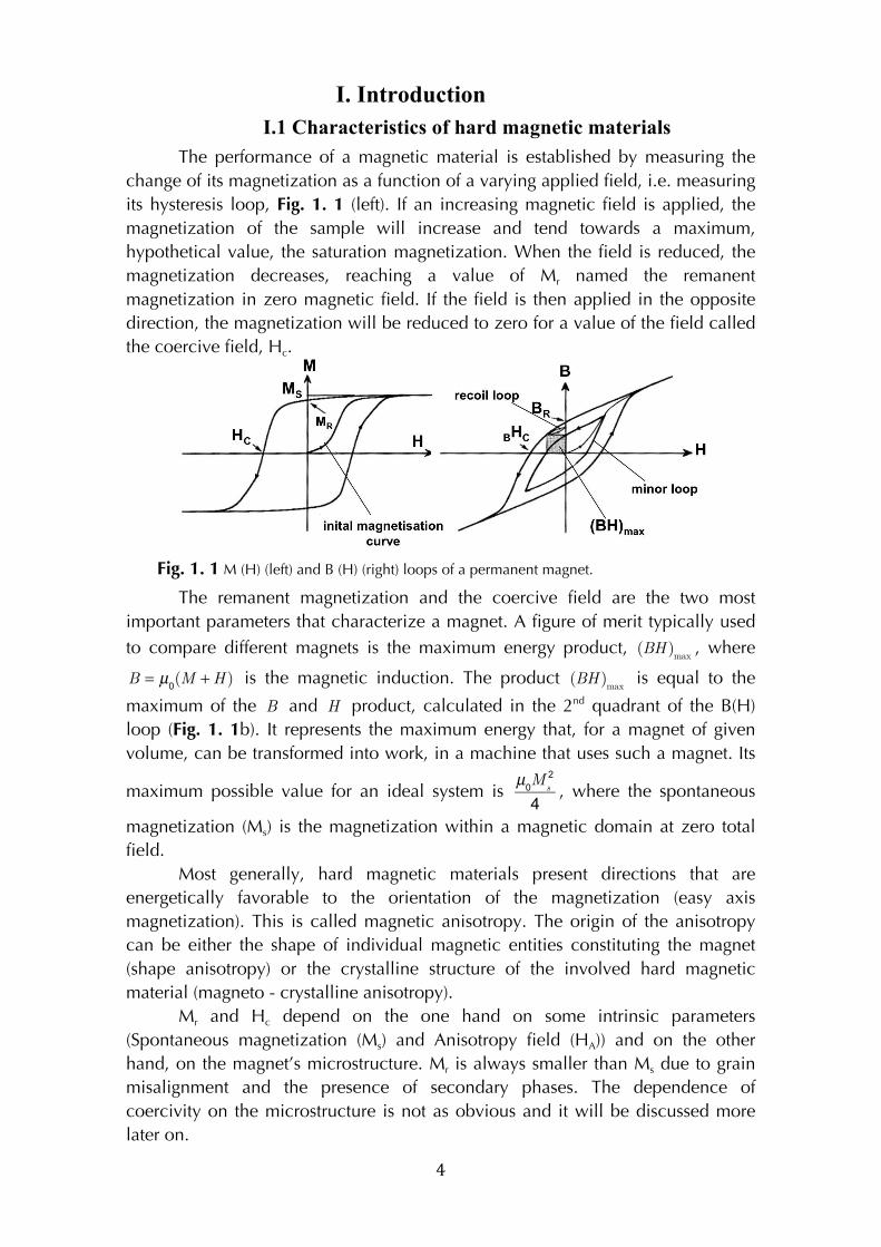
The performance of a magnetic material is established by measuring the

change of its magnetization as a function of a varying applied field, i.e. measuring

its hysteresis loop, Fig. 1. 1 (left). If an increasing magnetic field is applied, the

magnetization of the sample will increase and tend towards a maximum,

hypothetical value, the saturation magnetization. When the field is reduced, the

magnetization decreases, reaching a value of Mr named the remanent

magnetization in zero magnetic field. If the field is then applied in the opposite

direction, the magnetization will be reduced to zero for a value of the field called

the coercive field, Hc.

Fig. 1. 1 M (H) (left) and B (H) (right) loops of a permanent magnet.

The remanent magnetization and the coercive field are the two most

important parameters that characterize a magnet. A figure of merit typically used

to compare different magnets is the maximum energy product, (BH )

max, where

B = µ

0(M +H ) is the magnetic induction. The product

(BH )

max is equal to the

maximum of the B and H product, calculated in the 2nd quadrant of the B(H)

loop (Fig. 1. 1b). It represents the maximum energy that, for a magnet of given

volume, can be transformed into work, in a machine that uses such a magnet. Its

maximum possible value for an ideal system is

µ0M

s

2

4, where the spontaneous

magnetization (Ms) is the magnetization within a magnetic domain at zero total

field.

Most generally, hard magnetic materials present directions that are

energetically favorable to the orientation of the magnetization (easy axis

magnetization). This is called magnetic anisotropy. The origin of the anisotropy

can be either the shape of individual magnetic entities constituting the magnet

(shape anisotropy) or the crystalline structure of the involved hard magnetic

material (magneto - crystalline anisotropy).

Mr and Hc depend on the one hand on some intrinsic parameters

(Spontaneous magnetization (Ms) and Anisotropy field (HA)) and on the other

hand, on the magnet’s microstructure. Mr is always smaller than Ms due to grain

misalignment and the presence of secondary phases. The dependence of

coercivity on the microstructure is not as obvious and it will be discussed more

later on.

! 5!

I.2 Hard magnetic materials

The materials developed to produce permanent magnets are

(chronologically): steel alloys, Alnicos, ferrites and rare earth permanent magnets.

Before the ferrites were discovered, the magnets needed to be U - shaped,

horseshoe - shaped or in the form of long bars, in order to minimize the self-

demagnetizing field (shape anisotropy magnets). With the ferrites, which exploit

magneto-crystalline anisotropy, the shape constraint was eliminated since these

materials had, irrespective of their shape, coercivities bigger than their own

demagnetizing field.

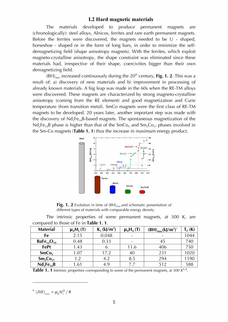
(BH)max increased continuously during the 20th century, Fig. 1. 2. This was a

result of: a) discovery of new materials and b) improvement in processing of

already known materials. A big leap was made in the 60s when the RE-TM alloys

were discovered. These magnets are characterized by strong magneto-crystalline

anisotropy (coming from the RE element) and good magnetization and Curie

temperature (from transition metal). SmCo magnets were the first class of RE-TM

magnets to be developed. 20 years later, another important step was made with

the discovery of Nd2Fe14B-based magnets. The spontaneous magnetization of the

Nd2Fe14B phase is higher than that of the SmCo5 and Sm2Co17 phases involved in

the Sm-Co magnets (Table 1. 1) thus the increase in maximum energy product.

Fig. 1. 2 Evolution in time of (BH)max.and schematic presentation of different types of materials with comparable energy density.

The intrinsic properties of some permanent magnets, at 300 K, are

compared to those of Fe in Table 1. 1.

Material μ0Ms (T) K1 (kJ/m3) μ0HA (T) (BH)max(kJ/m3)∗ TC (K)

Fe 2.15 0.048 - - 1044 BaFe12O19 0.48 0.33 - 45 740

FePt 1.43 6 11.6 406 750 SmCo5 1.07 17.2 40 231 1020

Sm2Co17 1.2 4.2 8.5 294 1190 Nd2Fe14B 1.61 4.9 7.7 512 588

Table 1. 1 Intrinsic properties corresponding to some of the permanent magnets, at 300 K1, 2.

!!!!!!!!!!!!!!!!!!!!!!!!!!!!!!!!!!!!!!!!!!!!!!!!!!!!!!!!

∗! (BH )

max= µ

0M

s

2 / 4 !

! 6!

I. 3 RE-Fe magnets

The outstanding properties of RE2Fe14B compounds are given mainly by the strong magneto-crystalline anisotropy provided by the RE element. As what concerns magnetization, the alloys formed with light rare earths (LREE) possess a high magnetization because the Fe magnetic lattice couples parallel with the RE magnetic lattice. On the contrary, the heavy rare earth elements (HREE) align anti-parallel with Fe giving a much-reduced overall magnetization17. However, HREE-TM alloys have the advantage of higher HA (e.g. HA (Dy2Fe14B) = 15 T; HA

(Nd2Fe14B) = 6.7 T). From all the possible compounds, the one with Nd, a LREE, has the

highest spontaneous magnetization. It implies that these magnets have the potential of achieving the highest maximum energy product.

The Nd2Fe14B compound crystallizes in a tetragonal structure, space group P42/mnm3,4,5. The lattice parameters are a = 8.8 Å and c = 12.2 Å6 and the magnetization easy axis is along c-axis above 135 K. The easy axis starts to tilt away from the c-axis below 135 K7,8. The angle between the easy axis and c-axis increases progressively from around 0° at T = 135 K to 30° at T = 4.2 K9.

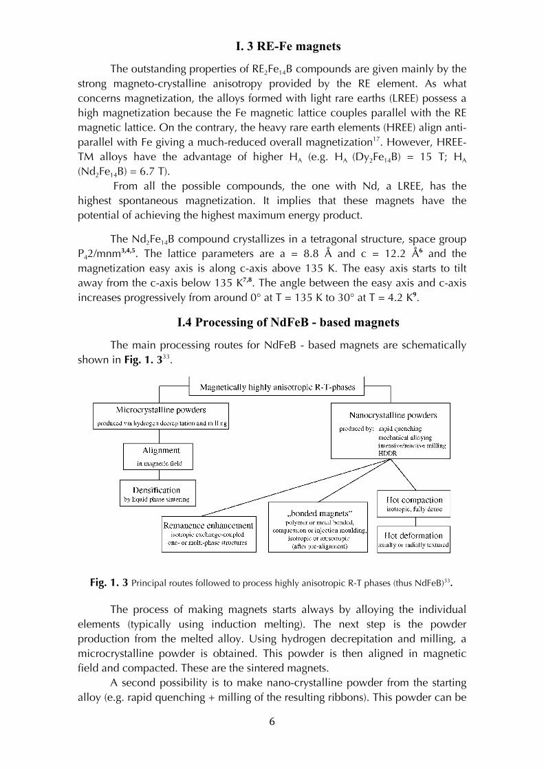
I.4 Processing of NdFeB - based magnets

The main processing routes for NdFeB - based magnets are schematically shown in Fig. 1. 333.

Fig. 1. 3 Principal routes followed to process highly anisotropic R-T phases (thus NdFeB)33.

The process of making magnets starts always by alloying the individual elements (typically using induction melting). The next step is the powder production from the melted alloy. Using hydrogen decrepitation and milling, a microcrystalline powder is obtained. This powder is then aligned in magnetic field and compacted. These are the sintered magnets.

A second possibility is to make nano-crystalline powder from the starting alloy (e.g. rapid quenching + milling of the resulting ribbons). This powder can be

! 7!

compacted as it is or mixed with a polymer (or a metal) producing the so-called

“bonded magnets”.

The highest (BH)max is obtained in anisotropic sintered NdFeB-magnets.

NdFeB has been prepared also in film form using both sputtering10,11,12,13,14

and Pulsed Laser Deposition15,16 techniques. Thin films have potential applications

in data storage, while thicker films are being developed for use in micro-systems.

The microstructure of the hard magnetic layer may be controlled to a certain

extent, through a control of preparation conditions. This allows an optimization of

the extrinsic properties, and makes films good candidates for studying

magnetization reversal.

I.5 NdFeB - based magnets. State of the art

Energy applications, like hybrid electric vehicles (HEV) and windmills, are

becoming more and more important. For permanent magnet based devices, there

is a need for magnetic materials with high (BH)max operational up to high

temperature (180 °C). As discussed previously, NdFeB magnets have the highest

(BH)max so they are appealing for this kind of application. The problem is that

above 100 °C, the coercivity of NdFeB is decreases rapidly with temperature so

that at the maximum working temperatures, the Hc of NdFeB is not sufficient. In

order to obtain enough coercivity at high temperatures, an increase of Hc at room

temperature is needed.

One way of improving coercivity of NdFeB-based magnets is to increase

the anisotropy field by adding HREE like Dy as Dy2Fe14B has much higher

anisotropy field than Nd2Fe14B. In this case, a part of Nd atoms in the 2:14:1

phase are replaced with Dy atoms. The inconvenience of Dy addition is the

decrease of saturation magnetization caused by the antiparallel alignement of Dy

magnetic moments and Fe magnetic moments17. The second problem with the Dy

is its cost, heavy rare earth, being more expensive than the light rare earths. In

this specific case, Dy is approximately 10 times more expensive than Nd. What is

more, Dy is a strategic element, with most of the known resources concentrated

in China.

In order to reduce the amount of Dy, the introduction of this element only

at the grain surface is a solution. In these magnets the reversal is thought to start at

defects present at grain boundaries. By increasing HA at the grain surface, the

coercivity should be increased. Two main techniques are used: the two powders

technique and grain boundary diffusion. In the first case, a mixture of two

powders (Nd2Fe14B-based powder and Dy-based powder) is generally aligned

under magnetic field, pressed, sintered at temperatures around 1000°C and

annealed at lower temperatures. The second powder can be for example

Dy2O318,19,20, DyHx

21, DyGa22 or Dy2S323. The resultant microstructure can be

considered as made of core-shell grains separated by secondary phases. The core

is typically 2:14:1 Dy- free, the shell 2:14:1 with some Nd atoms being replaced

by Dy atoms and the intergranular phases differ from one composition to another.

The thickness of the Dy-rich shell can, sometimes, be bigger than the size of the

Dy-free core in which case the amount of Dy is still high.

! 8!

In 2005, another technique, grain boundary diffusion (GBD) was

reported24,25. Dy-free sintered NdFeB-based magnets are coated with Dy-based

powders (Dy2O3, DyF3) and then heat-treated. In this case Dy is diffused along the

grain boundaries, forming a thin shell of (NdDy)2Fe14B around the Nd2Fe14B grains

and O and F form intergranular oxides with Nd. The thin shell has an increased

anisotropy and it has a positive effect on the Hc of these magnets. The amount of

Dy is significantly reduced compared to other techniques and the decrease of

remanent magnetization is almost zero. Hirota et al.25 report a decrease of Mr with

7% in the case of two powders technique and only 0.2% when GBD was used.

Alternatively, NdFeB-based magnets (with no Dy) were coated with a

sputtered layer of pure Dy and then annealed to allow Dy diffusion at the grain

interfaces26. Ding et al.27 reported an increase in coercivity with preservation of

remanence in magnets obtained by sintering of ribbons obtained from arc melting

of a NdFeB-based alloy. Prior sintering, the ribbons were immersed in a mixture

of DyF3 powder and ethanol, dried and annealed.

Recently, Li et al.28 studied the distribution of Dy in a commercial magnet

using SEM, TEM and 3DAP analysis. They suggest that the problem is not as

simple as thought. The increase of coercivity after addition of Dy might be due to

the anisotropy increase but not only. The intergranular phases are also different

(magnetically) and they could help in decoupling better the grains. It is clear that

the study related to Dy in NdFeB magnets is still an important one and efforts for

understanding in more detail what happens with Dy addition are still ongoing.

Another way of increasing the Hc is by improving the microstructure. It is

known that the coercivity increases when the grain size decreases (down to a few

10’s of nm). In sintered magnets, below 3 μm grain size the coercivity is lowered

due to oxidation. Using the so-called pressless process (PLP), Sagawa et al.

managed to obtain magnets with high Hc and grain size < 3 μm under Ar

atmosphere29.

In magnets based on NdFeB the intergranular phases play an important

role. There are two major types of secondary phases considered 30: i) very thin (1-

2 nm) metallic Nd-rich phases separating the main phase grains and ii) crystalline

oxides (Nd2O3, NdO)31 at triple junction points.

The exact chemical composition of the first type of secondary phase is

difficult to identify, considering the small sizes implied. Nevertheless, important

progress was made in the last years due to high-resolution characterization

techniques like TEM and atom probe. It is commonly believed that the thin layer

separating neighboring grains is non-magnetic and it enhances coercivity via

magnetic decoupling of the grains32,33,34. More recently, Sepehri-Amin et al.35

detected iron in the thin grain boundary using atom probe elemental analysis.

They prepared a thin layer of the same composition as the one detected at the

grain boundaries and they concluded that the phase is a soft magnetic one with a

saturation magnetization of ≈ 440 emu cm-3. In this case, the magnetization

reversal mechanism must be different. They suggest that the 2:14:1 grains are

magnetically coupled via the grain boundary phase which act to pin domain

walls.

! 9!

The coercivity of NdFeB - based magnets can be also increased by

improving the magnetic decoupling of the 2:14:1 phase. This is typically done by

adding non - magnetic elements that preferentially stay at the grain boundary. The

most used element for this purpose is Cu.

The effect of Cu on the magnetic properties of NdFeB was already studied

in different kinds of magnets: i) sintered magnets obtained starting from a

NdFeBCu-based powder36,37,38,39; ii) sintered magnets obtained starting from a

mixture of NdFeB - based powder and Cu powder40,41,42,43,44,45. The general

conclusion of all of these studies, indifferent of the exact composition, starting

powder size, final grain size etc. is the same: the addition of Cu improves

coercivity of NdFeB-based magnets by the formation of additional inter-granular

phases (with Nd and/or O) that decouple the 2:14:1 grains. The presence of the

low temperature eutectic NdCu2 facilitates the formation of a continuous inter-

granular phase. Recently, S. Sepehri-Amin et al., reported another way of

introducing Cu in the magnets, using NdCu powder46. They start from a mixture of

NdFeB-based and NdCu powders and get magnets with 2:14:1 nano-sized grains

enveloped in a Nd-rich (Cu containing) phase. Coercivity of 2.6T was obtained.

The Toyota Motor Corporation developed the so-called infiltration process in

order to introduce Cu to the Nd-rich grain boundaries47. Details about this process

are given in chapter III.

It is clear that the microstructure has a decisive role in the coercivity

mechanism of NdFeB-based magnets. Nevertheless, the exact nature of the

microstructure - coercivity link is not understood and as already mentioned, its

study has been one of the important objectives of this thesis.

! 10!

!!!!!!!!!!!!!!!!!!!!!!!!!!!!!!!!!!!!!!!!!!!!!!!!!!!!!!!!

1 J. M. D. Coey, Magnetism and Magnetic materials book, Cambridge, 2010, 614p;

2 C. Ndao , PhD thesis (2010);

3 J. F. Herbst, J. J. Croat, F. E. Pinkerton and W. B. Yelon, Phys. Rev. B 29, 4176 (1984);

4 D. Givord, H. S. Li and J. M. Moreau, Sol. State Comm. 50, 497 (1984);

5 C. B. Shoemaker, D. P. Shoemaker and R. Fruchart, Acta Cryst. C 40, 1665 (1984);

6 C. Abache and H. Oesterreicher, J. Appl. Phys. 57, 4112 (1985);

7 D. Givord, H. S. Li, J. M. Moreau, R. Perrier de la Bâthie and E. Du Trémolet de Lacheisserie, Physica B 130, 323 (1985);

8 D. Givord, H. S. Li and R. Perrier de la Bâthie, Sol. State Comm. 51, 857 (1984);

9 M. Sagawa, S. Fujimura, H. Yamamoto, Y. Matsuura and S. Hirosawa, J. Appl. Phys. 57(1), 4094 (1985);

10 F. J. Cadieu: In Physics of Thin Films, Francombe, M., Vossen, J. (eds.) vol. 16, Academic Press Inc., (1992);

11 B. A Kapitanov, N.V Kornilov, Ya. L Linetsky and V. Yu Tsvetkov, JMMM 127, 289-297 (1993);

12 S. Parhofer, G. Gieres, J. Wecker, and L. Schultz, J. Magn. Magn. Mater. 163, 32 (1996);

13 L. K. E. B. Serrona, R. Fujisaki, A. Sugimura, T. Okuda, N. Adachi, H. Ohsato, I. Sakamoto, A. Nakanishi, M. Motokawa, D. H. Ping, and K. Hono, J. Magn. Magn. Mater. 260, 406 (2003);

14!N. M. Dempsey, A. Walther, F. May and D. Givord, Appl. Phys. Lett. 90, 092509 (2007);!

15!U. Hannemann, S. Fähler, V. Neu, B. Holzapfel, and L. Schultz, Appl. Phys. Lett. 82, 3710 (2003);

16 Nakano, M., Katoh, R., H. Fukunaga. Fabrication of Nd–Fe–B Thick-Film Magnets by High-Speed PLD Method. IEEE Trans. Magn. 39, 2863-2865 (2003);

17 I. A. Campbell, J. Phys. F 2, L47 (1972);

18 M. Doser and G. Keeler, J. Appl. Phys. 64, 5311 (1988);

19 F. Z. Lian, L. Ai, X. S. Zhang and H. H. Zhao, JMMM 127, 190 (1993);

20 L. Li, J. Yi, Y. Peng and B. Huang, JMMM 308, 80 (2007);

21 R.S. Mottram, A. Kianvash and I. R. Harris, J. Alloys Comp. 283, 282(1999);

! 11!

!!!!!!!!!!!!!!!!!!!!!!!!!!!!!!!!!!!!!!!!!!!!!!!!!!!!!!!!

22 C.H. de Groot, K. H. J. Buschow, F. R. de Boer and K. de Kort, J. Appl. Phys. 83, 388 (1998);

23 A. M. Gabay, M. Marinescu, W. F. Li, J. F. Liu and G. C. Hadjipanayis, J. Appl. Phys. 109, 083916 (2011)

24 H. Nakamura, K. Hirota, M. Shimao, T. Minowa and M. Honshima, IEEE Trans. Magn. 41, 3844 (2005);

25 K. Hirota, H. Nakamura, T. Minowa and M. Honshima, IEEE Trans. Magn. 42, 2909 (2006);

26 D. Li, S. Suzuki, T. Kawasaki and K-i. Machida, Jpn. J. Appl. Phys. 47, 7876 (2008);

27 Y. Ding, R. J. Chen, Z. Liu, D. Lee and A. R. Yan, J. Appl. Phys. 107, 09A726(2010);

28 W.F. Li, H. Sepehri-Amin, T. Ohkubo, N. Hase and K. Hono, Acta Mat. 59, 3061 (2011);

29 M. Sagawa, in: S. Kobe, P.J. McGuinness (Eds.), Proceedings of the 21st Workshop on Rare-Earth Permanent Magnets and their Applications, Jozef Stefan Institute, Ljubliana, Slovenia, p183 (2010);

30 T. G. Woodcock, Y. Zhang, G. Hrkac, G. Ciuta, N. M. Dempsey, T. Schrefl, O. Gutfleisch and D. Givord, Scripta Materialia 67, 536 (2012);

31 T. G. Woodcock and O. Gutfleisch, Acta Mat. 59, 1026 (2011);

32 M. Sagawa, S. Fujimura, N. Togawa, H. Yamamoto and Y. Matsuura, J. Appl. Phys. 55(6), 2083 (1984);

33 O. Gutfleisch, J. Phys. D: Appl. Phys. 33, R157 (2000);

34 F. Vial, F. Joly, E. Nevalainen, M. Sagawa, K. Hiraga and K. T. Park, JMMM 242, 1329 (2002);

35 H. Sepehri-Amin, T. Ohkubo, T. Shima and K. Hono, Acta Mat. 60, 819 (2012); !

36 A. Kianvash and I. R. Harris, J. Appl, Phys. 70, 6453 (1991);

37 H. J. Engelmann, A. S. Kim and G. Thomas, Scripta Materialia 36, 55 (1997);

38 H. Lemke and G. Thomas, Scripta Materialia 37, 1651 (1997);

39 S. Pandian, V. Chandrasekaran, G. Markandeyulu, K. J. L. Iyer and K. V. S. Rama Rao, J. Appl. Phys. 92, 6082 (2002);

40 O.M. Ragg and I. R. Harris, J. Alloys Comp. 256, 252 (1997);

41 A. Yan, X. Song, Z. Chen and X. Wang, JMMM 185, 369 (1998);

42 R. S. Mottram, A. J. Williams and I. R. Harris, JMMM 234, 80 (2001);

! 12!

!!!!!!!!!!!!!!!!!!!!!!!!!!!!!!!!!!!!!!!!!!!!!!!!!!!!!!!!

43 X. G. Cui, M .Yan, T. Y. Ma and L. Q. Yu, Phys. B 403, 4182 (2008);

44 P. Yi, M. Lin, R. Chen, D. Lee and A. Yan, J. Alloys Comp. 491, 605 (2010);

45 C. Sun, W. Q. Liu, H. Sun, M. Yue, X. F. Yi and J. W. Chen, J. Mater. Sci. Technol. 28, 927 (2012);

46 H. Sepehri-Amin, D. Prabhu, M. Hayashi, T. Ohkubo, K. Hioki, A. Hattori and K. Hono, Scripta Mat. 68, 167 (2013);

47 A. Kato, S. Tetsuya, S. Noritsugu, K. Hideshi and S. Takashi (Toyota Motor Corporation), High coercive field NdFeB magnet and construction method therefor, JP2010010665 (2010).

!

! 13!

II. Theory of Coercivity

II.1 Origin of Coercivity. Anisotropy.

Coercivity characterizes the resistance of a ferromagnetic (or ferrimagnetic)

material to demagnetization. The coercive field refers to the magnetic field

needed to bring the magnetization to zero, along a certain direction, once it was

previously saturated along that direction.

The classification of magnetic materials into “hard” or “soft” materials is

based on the value of the coercive field. The present work is concentrated on

hard magnetic materials with Hc values typically higher than 0.1 T.

The intrinsic parameter that governs coercivity is the magnetic anisotropy,

which implies the existence of energetically favorable directions for

magnetization either related to the crystalline axes – magneto-crystalline

anisotropy - or related to the macroscopic shape of the sample – shape

anisotropy. The axis corresponding to the lower energy state is called the easy

axis while that corresponding to high energy is the hard axis. The physics of

anisotropy is explained in several books like for example the ones of G. Bertotti1,

R. Skomski and J.M.D. Coey2 or lectures of P. Bruno3.

Further, the case of uni-axial systems with strong anisotropy will be treated

since the materials we are studying enter into this category. In this type of system,

there is only one easy axis and the anisotropy energy density is approximated to:

!

E(θ) = K1sin2

θ +K2sin4

θ +K3sin6

θ + ...!

(2. 1)

where K

iis the i -th order anisotropy constant and θ is the angle between the

magnetization and the easy axis. Generally, only the first term is considered but

there are special cases where the next terms become important as well, especially

at low temperature. If (2. 1) is reduced to the first term and K

1> 0 , two equivalent

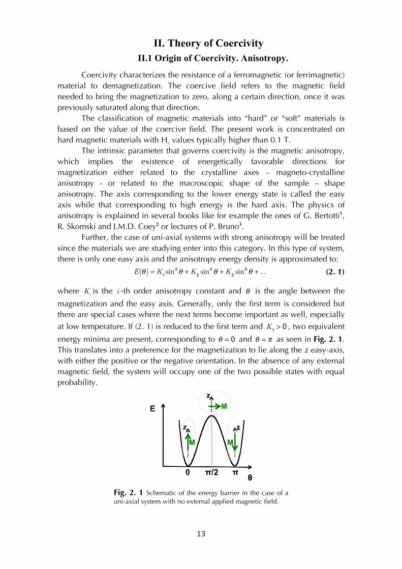
energy minima are present, corresponding to θ = 0 and θ = π as seen in Fig. 2. 1.

This translates into a preference for the magnetization to lie along the z easy-axis,

with either the positive or the negative orientation. In the absence of any external

magnetic field, the system will occupy one of the two possible states with equal

probability.

!

Fig. 2. 1 Schematic of the energy barrier in the case of a uni-axial system with no external applied magnetic field.

! 14!

The two energy minima are separated by a maximum, at θ = π 2 . This

corresponds to a magnetization hard axis and the energy needed to align the

magnetization along any direction perpendicular to the easy axis, is the

anisotropy energy.

Consider now that the magnetization is aligned along the easy axis at θ = 0

and a magnetic field is applied along the same axis, at θ = π . In the Stoner-

Wohlfarth model, the magnetization is assumed to rotate uniformly. The

associated energy becomes:

! E(θ) = K

1sin2

θ + µ0M

sH cosθ ! (2. 2)

where Ms is the spontaneous magnetization and H the applied magnetic field.

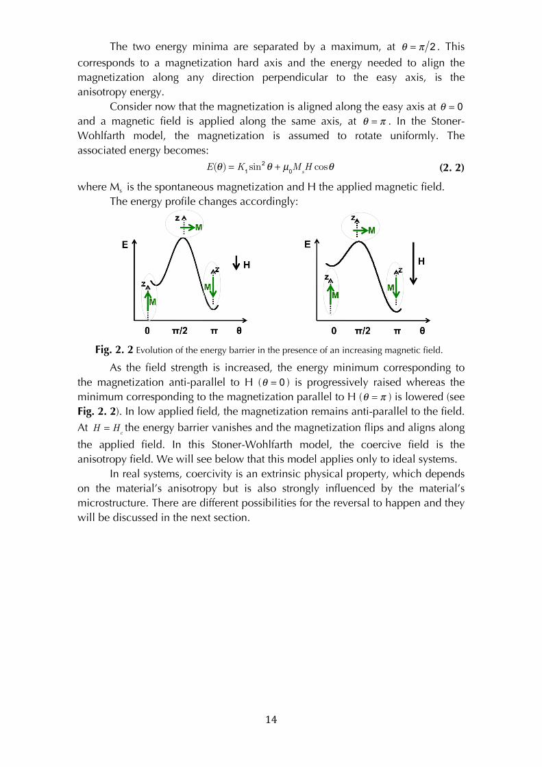
The energy profile changes accordingly:

! !

Fig. 2. 2 Evolution of the energy barrier in the presence of an increasing magnetic field.

As the field strength is increased, the energy minimum corresponding to

the magnetization anti-parallel to H ( θ = 0 ) is progressively raised whereas the

minimum corresponding to the magnetization parallel to H (θ = π ) is lowered (see

Fig. 2. 2). In low applied field, the magnetization remains anti-parallel to the field.

At H = H

cthe energy barrier vanishes and the magnetization flips and aligns along

the applied field. In this Stoner-Wohlfarth model, the coercive field is the

anisotropy field. We will see below that this model applies only to ideal systems.

In real systems, coercivity is an extrinsic physical property, which depends

on the material’s anisotropy but is also strongly influenced by the material’s

microstructure. There are different possibilities for the reversal to happen and they

will be discussed in the next section.

!

! 15!

II.2 Types of magnetization reversal in uniaxial high anisotropy

systems

!

II.2.1 Nucleation

Nucleation implies the occurrence of instabilities in a saturated magnetic

state for a certain value of an applied field, HN, the nucleation field. In the Stoner-

Wohlfarth model, discussed briefly in the first part of this section, the coercive

field is equal to the nucleation field. In real systems, reversal begins at defects and

it may be decomposed into two stages, nucleation and propagation. The larger of

these two fields determines the value of the coercive field. Two cases of

nucleation type reversal will be presented and the formula for the corresponding

nucleation field will be given.

Coherent rotation. Stoner-Wohlfarth model.

In the Stoner-Wohlfarth (SW) model4, the magnetization can be considered

homogeneous and the magnetic moments parallel at any moment. The model is

valid in particular for very small magnetic particles.

We consider that the easy axis is the z-axis and it coincides with the

direction of the applied field. The energy density is given by equation (2. 2).

The system will “look for” the position where its energy is minimized.

Accordingly, the equality ∂E / ∂θ = 0 gives:

! 2K

1sinθ cosθ − µ

0M

sH sinθ = 0 !

sinθ(2K

1cosθ − µ

0M

sH ) = 0 !

(2. 3) !

Considering that the nucleation field, at which the first instability in the

moment configuration will occur, corresponds to E

min= E

max, one gets:

!

Hn=

2K1

µ0M

s

! (2. 6)

which is the anisotropy field.

Full reversal follows nucleation. Thus, for coherent rotation, the coercive

field, identical to the nucleation field, is equal to the anisotropy field. It considers

that going from one easy direction to the other, the magnetization changes just

the direction, not its magnitude and it is obliged to pass through the hard axis

magnetization, thus it has to pay the anisotropy field in order to arrive in the next

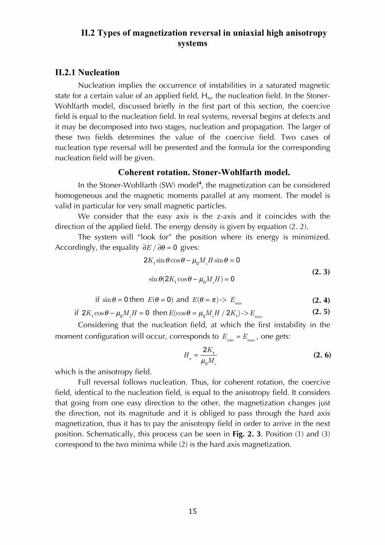
position. Schematically, this process can be seen in Fig. 2. 3. Position (1) and (3)

correspond to the two minima while (2) is the hard axis magnetization.

! !

if sinθ = 0 then E(θ = 0) and

E(θ = π)-> E

min

if 2K

1cosθ − µ

0M

sH = 0 then

E(cosθ = µ

0M

sH / 2K

1)->

E

max

(2. 4)

(2. 5)

! 16!

!

Fig. 2. 3 Schematic representing coherent rotation in uni-axial systems.

All that was mentioned about coherent rotation is valid for the case where

the field is applied along the easy direction. Interesting information can be

extracted if the field is applied along other directions. This topic will be discussed

in one of the next sections, where the angular dependence of coercivity for

different types of reversal will be presented.

Magnetization curling

Another nucleation type of magnetization reversal is the one called

magnetization curling. Contrary to the SW model, the magnetization does not

remain homogeneous during rotation. Flux closure occurs to reduce the

magnetostatic energy. While in the case of coherent rotation the exchange energy

was totally ignored, in this case, the exchange energy has to be paid but it is

compensated by the gain in magnetostatic energy.

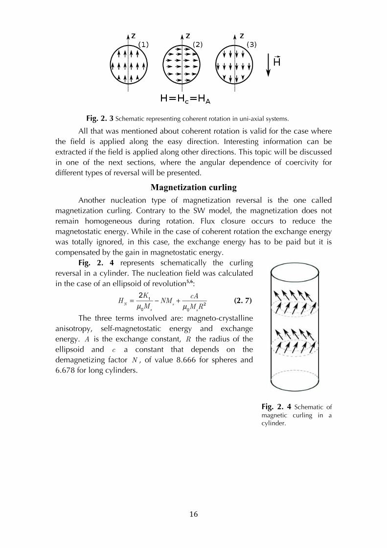
Fig. 2. 4 represents schematically the curling

reversal in a cylinder. The nucleation field was calculated

in the case of an ellipsoid of revolution5,6:

HN=

2K1

µ0M

s

−NMs+

cA

µ0M

sR

2! (2. 7)

The three terms involved are: magneto-crystalline

anisotropy, self-magnetostatic energy and exchange

energy. A is the exchange constant, R the radius of the

ellipsoid and c a constant that depends on the

demagnetizing factor N , of value 8.666 for spheres and

6.678 for long cylinders.

!!

Fig. 2. 4 Schematic of magnetic curling in a cylinder.

! 17!

II.2.2 Nucleation versus Pinning

For very high anisotropy systems, the difference in calculated coercive field

values for coherent rotation and curling are minor. Nevertheless, the coercivity

values measured experimentally are always smaller than the values given by both

the coherent rotation model and the curling model. This is the so-called Brown

paradox and can be explained by the fact that the microstructure has a strong

influence on coercivity. In reality, the presence of areas with lower anisotropy

decreases a lot the value of the coercive field. Nucleation starts at the lower

anisotropy regions and it will then propagate into the entire structure that is in

contact with that zone. So, a small defect can induce the reversal of an important

part of the system. After it nucleates, reversal may propagate in the entire system,

for the same field. In this case, reversal is controlled by nucleation. Alternatively,

the nucleus formed may remain pinned at magnetic heterogeneities, in which

case reversal is said to be pinning controlled.

In this context, nucleation consists in the formation, under a certain

applied field, of small nuclei (domains) with reversed magnetization separated,

via domain walls or domain wall like moment configurations, from the rest of the

material, which is still in its saturated state. After nucleation, the formed nucleus

may: i) disintegrate spontaneously (if the energy is not enough to maintain it); ii)

remain pinned or iii) grow into the rest of the magnetic body. In this latter case,

the propagation of magnetization reversal through the entire system proceeds for

the same field value as nucleation occurs. This corresponds to the case of

nucleation type materials, which are essentially homogeneous in the bulk. The

domain wall energy does not depend on its position and the nucleus of reversed

magnetization formed initially, grows to encompass the entire material, thus

minimizing Zeeman energy.

Conversely, it may happen that the growth of reversed domains is impeded

by some inhomogeneities in the material. In this case, the domain wall may be

trapped at some low energy defect region and an increased value of the applied

field is needed in order to be able to move further the domain wall. This is the

case of domain wall pinning. It is obvious that the pinning mechanism implies the

existence of reversed magnetic domains (related to the saturated state) so we

could say that there are no purely pinning type materials since we need to

produce, one way or another, some reversed regions.

So, we have a system decomposed into domains, with alternating

magnetization orientations, separated by magnetic domain walls. A domain wall

can be imagined as a membrane that can be moved using the Zeeman energy due

to the applied field. Its energy, for uniaxial systems considered here, is

γ = 4 AK

1. This membrane can move freely until it encounters some pinning

defects with, for instance, K1 smaller than the value of the base material. At that

point, the wall is stuck, the position being energetically favorable. In order to

move the wall further, the applied field must be increased. The concept of

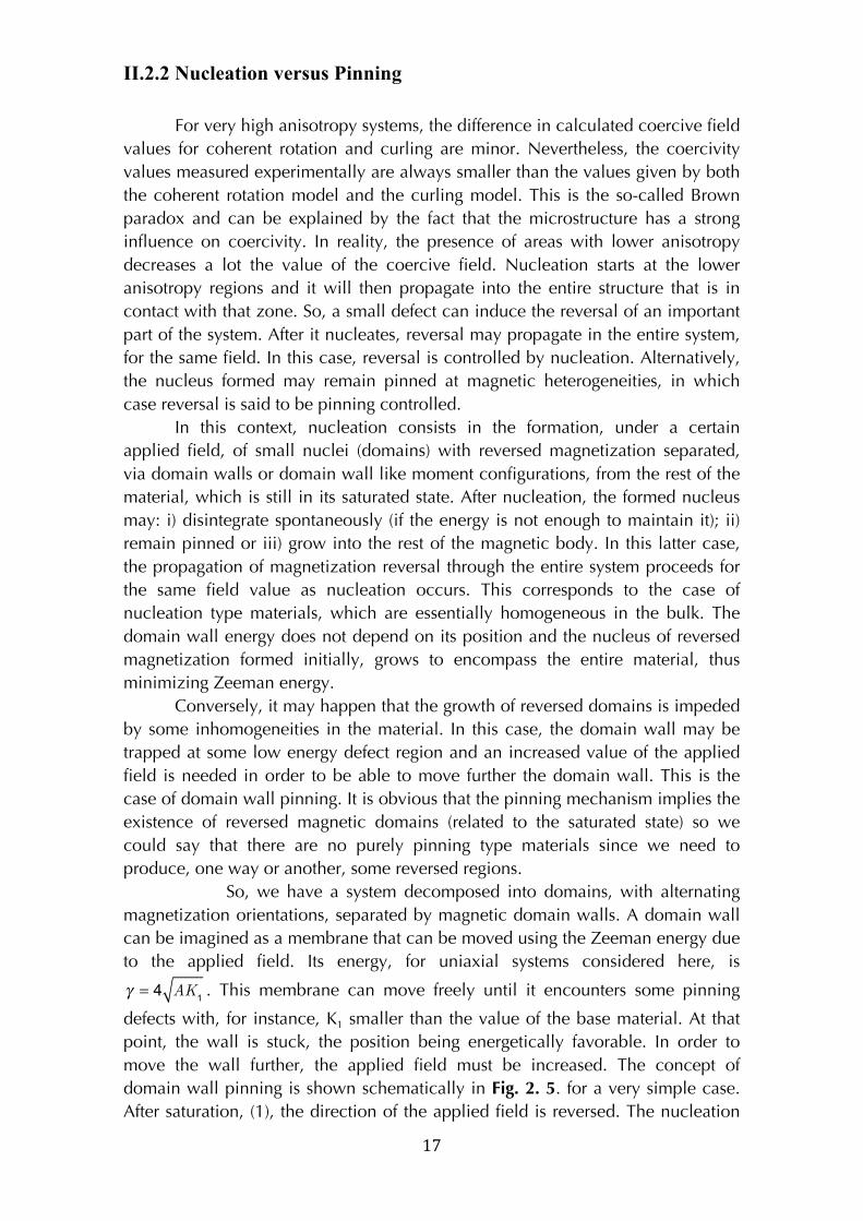
domain wall pinning is shown schematically in Fig. 2. 5. for a very simple case.

After saturation, (1), the direction of the applied field is reversed. The nucleation

! 18!

starts at (2), the domain wall is formed, it starts to move but at (3) it encounters

some defect points and is trapped there. A

bigger value of the field unblocks the wall and

in (4) saturation in the opposite direction is

achieved.

There are different pinning modes

depending on the domain wall characteristics

(energy, width, magnetic properties), pinning

site characteristics (dimensionality: point or

planar, magnetic nature) and the way they

interact with each other.

Friedberg and Paul7 and Hilzinger and

Kronmüller8 calculated the pinning field

defined as the maximum applied field for

which there exists a static domain wall solution in the case of a magnetic planar

defect (grain boundary) and a 180° domain wall:

!

Hp= 3

−3/2K

1

Ms

dw

δw

(A

1

A1

'−

K1

'

K1) ! (2. 8)

Here, K1, Ms, A1, are the anisotropy constant, spontaneous magnetization,

exchange constant characterizing the material outside the domain wall and A1’,

K1’ are the exchange constant and anisotropy constant related to the defect. dw

and δw represent the widths of the defect and of the domain wall, respectively.

Kronmuller et al.9 calculated the field for point defects:

!

Hc=

1

Ms

(K

1

δw

1/2+

A

δw

5/2)ρ1/2

! (2. 9)

with ρ the defect density and all the other parameters characterizing the main

phase.

As a general rule, the pinning is believed to be more effective for defects

comparable in size with the domain wall width and for domain walls where K1

varies drastically with the position.

In conclusion, defects can have both a positive and a negative effect on the

value of the coercivity. When they serve as nucleation points, they represent

weak points of a magnet while, when playing the role of pinning sites, they can

retard the reversal to higher applied fields, thus increasing the resistance to

demagnetization.

In some cases, the defect region source of domain wall pinning may be

associated to the same defect that is the source of nucleation. Then, the volume of

magnetization reversed at nucleation is extremely small, not detectable by

magnetization measurements. It is not possible to separate experimentally such

pinning-controlled coercivity from true nucleation. In this case, Givord and

Rossignol10 proposed to use the expression “passage” rather than “pinning”.

!

!

Fig. 2. 5 Depiction of magnetization reversal in the case of nucleation-pinning reversal mechanism.

! 19!

II.3 Methods to characterize coercivity

In the previous paragraphs, different types of magnetization reversal were

presented. Considering the experimental results in the case of uniaxial high

anisotropy systems, we can say that the mechanism of coercivity is a complex one

that implies more than one, possibly all of the above mentioned events:

nucleation at lower anisotropy defect points, formation of domain walls,

propagation of these domain walls into the main phase, pinning – depinning in

the case of inhomogeneous materials. Each of these events takes place for a

certain value of the external applied field, the highest of them being the coercive

field. Understanding why a certain process happens for that certain field and

relating it to the microstructure is an important and difficult problem in permanent

magnet research. Knowing how the microstructure should be optimized and

doing so, one can exploit better the intrinsic properties of the given material.

Why is this problem difficult? Because it is impossible to probe directly the

microstructure-reversal link, the critical lengths implied being too small to be

accessible to experiment. That’s why indirect measurements are used to study this

problem. The most important ones, that will be discussed further, are:

a) Temperature and time dependence of coercivity; b) Angular dependence of coercivity; c) Minor loop analysis.

II.3.1 Temperature and time dependence of coercivity

Hysteresis loops measured at different temperatures on NdFeB-based

magnetic materials show a continuous decrease of coercivity with increasing

temperature. The rate of the decrease may vary from one material to another as

shown for ex. in 11,12.

Starting from Hc(T) measurements, different models are being used to

analyze the magnetization reversal type.

The most used approach to analyze Hc(T) is the so-called micromagnetic

model (MM). In the framework of this model, the coercive field was found to have

the form:

!

Hc= α

2K1

µ0M

s

−Neff

Ms! (2. 10)

Expression (2. 10) was initially introduced on purely phenomenological

grounds13,14. Kronmüller and co-workers15 showed that the above mentioned

equation may be derived from linearization of the classical micro-magnetic

equations in the case of inhomogeneous systems, characterized by a strong

magneto-crystalline anisotropy with local deviations of the anisotropy constant.

Nucleation reversal starts at points where anisotropy is a fraction of the anisotropy

of the bulk. The parameter α in eq. (2. 10) indicates how much the anisotropy is

lowered in the nucleation starting points.

In 16, Hc(T) is treated considering three regions of temperature. The regions

are chosen knowing that in the Nd2Fe14B system, there is a spin reorientation at

around 135 K and the anisotropy changes from uni-axial to cone like.

! 20!

a) 135 K < T < 460 K

!

Hc= α

Kα

ψ

min2K

1

Ms

−Neff

Ms! (2. 11)

α

K is a structure related parameter that was calculated in the case of a

2r

0

width planar inhomogeneity with no anisotropy, as being:

!

αK= 1−

1

4π2

δw

2

r0

2(−1+ 1+

4K1r

0

2

A)2! (2. 12)

If 2πr

0≥ δ

w and the defect has no anisotropy, then (2. 12) becomes:

!

αK=

δw

πr0

! (2. 13)

α

ψ

min corresponds to

ψ ≅π

4 and it is derived from:

!

αψ=

1

cosψ

1

(1+ tg2/3ψ )3/2

(1+2K

2

K1

tg2/3ψ

1+ tg2/3ψ

) ! (2. 14)

It takes into consideration the grain misalignment, ψ being the angle

between the c-axis of the grain and the applied field.

Equation (2. 11) can be re-written as:

!

Hc

Ms

= αKα

ψ

min2K

1

Ms

1

Ms

−Neff! (2. 15)

The plot

Hc

Ms

vs.

αKα

ψ

min2K

1

Ms

will have a linear behavior and the values for

αK and Neff can be extracted. Knowing α

K, r

0 results naturally from (2. 13).

b) T < 135 K

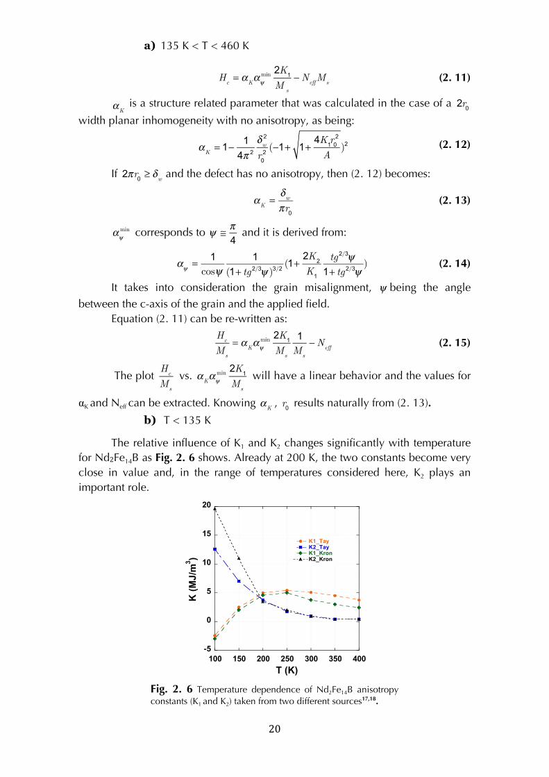
The relative influence of K1 and K2 changes significantly with temperature

for Nd2Fe14B as Fig. 2. 6 shows. Already at 200 K, the two constants become very

close in value and, in the range of temperatures considered here, K2 plays an

important role.

-5

0

5

10

15

20

100 150 200 250 300 350 400

K1_TayK2_TayK1_KronK2_Kron

K (

MJ

/m3)

T (K)!

Fig. 2. 6 Temperature dependence of Nd2Fe14B anisotropy constants (K1 and K2) taken from two different sources17,18.

! 21!

The coercive field is then:

!

Hc= α

' 4

3

K2

61/2

Ms

(K

1+ 2K

2+K

d

K2

)3/2! (2. 16)

where K

d=

1

2M

s

2(N⊥−N

) 15and α

' encompasses the effect of grain

surfaces. This last parameter can be extracted, like in the previous case, by

plotting the right graph.

c) T > 460K

At these high temperatures, K1 and K2 have very low values and the

coercivity is mainly due to domain wall pinning. For planar defects:

!

Hc=

2δw

3πr0

2K1

Ms

−NMs! (2. 17)

The plot

Hc

Ms

vs.

2K1

Ms

2provides the values for N and r0.

Briefly resumed, in many publications, the coercive field is simply

expressed as in (2. 10). Neff and α are considered as temperature independent

parameters even if, strictly speaking, they are not. Values of α > 0.3 are taken as

proof that reversal occurs by nucleation11, since the micromagnetic model as

developed, predicts that in this case, the nucleation field is larger than the

propagation field.

A second model, called the Global Model (GM) was proposed by Givord

et al.19, 20. It does not relate the coercivity directly to the anisotropy of the main

phase. The concept of activation volume is introduced and the coercivity is

related to this parameter that can be accessed experimentally.

The GM states that reversal is initiated in a critical volume, v

n

, with the

formation of a heterogeneous magnetic configuration, reminiscent of a domain

wall, of energy γ

n

, under a critical field:

!

Hcrit

= α ' γn

vn

1/3µ0M

s

! (2. 18)

α' being a phenomenological parameter and

M

s the spontaneous

magnetization of the main phase.

Thermal activation is also considered, at finite temperatures. In this case:

!

vn= v

a=

kBT

SvM

s

! (2. 19)

S

v is the viscosity coefficient, experimentally accessible from magnetic

after-effect measurements. This will be discussed further at the end of this chapter.

Further assumptions:

v

n

(critical volume), assumed to be proportional to δ

n

3 (domain wall width

in critical volume) is the critical volume in which reversal is initiated, assumed to

be equal to the experimentally derived activation volume v

a

;

γ

n (wall energy in critical volume) assumed proportional to γ (wall energy

main phase);

! 22!

A

n (exchange constant in critical volume) assumed to be proportional to A

(exchange constant of the main phase).

The coercive field is expressed as:

!

Hc= α

γ

va

1/3µ0M

s

−NMs− 25S

v! (2. 20)

Using the notation H

0= H

c+ 25S

v , equation (2. 20) becomes:

!

H0= α

γ

va

1/3µ0M

s

−NMs!

(2. 21)

or

H0

Ms

= αγ

va

1/3µ0M

s

2−N ! (2. 22)

The two parameters: α and N can be extracted by plotting

H0

Ms

vs.

γ

va

1/3µ0M

s

2.

To conclude this section, it can be noted that both the MM (2. 10) and GM

models (2. 20) assume simple proportionality between an intrinsic property of the

main phase (K or γ ) and the same property in the defect region.

An interesting aspect of the global model emerges in the case where the

anisotropy may be expressed in terms of 2nd order anisotropy only:

va δ

n

3≈ (

An

Kn

)3/2=> K

n

An

va

2/3

γn A

nK

n

An

va

1/3

Eq. (2. 18) becomes:

!

Hcrit α

' An

va

2/3M

s

= αA

va

2/3M

s

! (2. 23)

In expression (2. 23), the contribution of anisotropy is implicitly included

in the activation volume, an experimental quantity. An expression for the

temperature dependence of the coercive field is obtained which does not rely on

the hypothesis that the anisotropy (or the domain wall energy) in the defect region

is proportional to the main phase anisotropy. This relation can not be used in the

case of NdFeB magnets where higher order anisotropy constants must be

considered, in particular at low temperature.

Magnetic viscosity

Magnetic viscosity measurements give access to the activation volume, a

parameter used into the global model just described. When the system is in a

metastable state and this state is separated from lower energy states by energy

barriers of the same order of magnitude as the thermal energy, thermal activation

will contribute to magnetization reversal. The energy landscape is fixed and a

certain characteristic time τ is needed for the progressive rearrangement of the

magnetic structure to be produced and states with lower energy to be reached.

This time is given by the Arrhenius law:

! 23!

!

τ = τ

0e

Ea

kBT

! (2. 24)

τ0 is a constant of the order of 10-10 seconds and E

a is the characteristic height of

the barriers that will be surpassed after time τ . The bigger the ratio between

E

aand the thermal energy, the longer the time spent in front of these barriers.

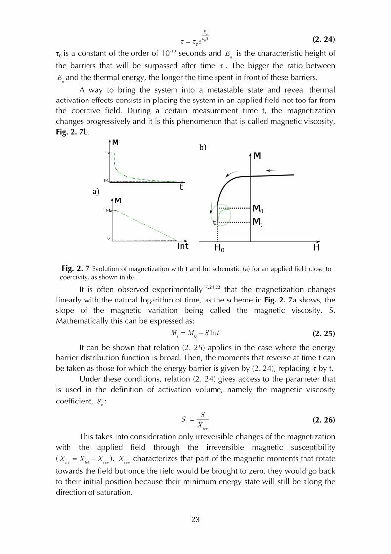
A way to bring the system into a metastable state and reveal thermal

activation effects consists in placing the system in an applied field not too far from

the coercive field. During a certain measurement time t, the magnetization

changes progressively and it is this phenomenon that is called magnetic viscosity,

Fig. 2. 7b.

a)

!

b)

!

Fig. 2. 7 Evolution of magnetization with t and lnt schematic (a) for an applied field close to coercivity, as shown in (b).

It is often observed experimentally17,21,22 that the magnetization changes

linearly with the natural logarithm of time, as the scheme in Fig. 2. 7a shows, the

slope of the magnetic variation being called the magnetic viscosity, S.

Mathematically this can be expressed as:

! M

t= M

0− S ln t ! (2. 25)

It can be shown that relation (2. 25) applies in the case where the energy

barrier distribution function is broad. Then, the moments that reverse at time t can

be taken as those for which the energy barrier is given by (2. 24), replacing τ by t.

Under these conditions, relation (2. 24) gives access to the parameter that

is used in the definition of activation volume, namely the magnetic viscosity

coefficient, S

v:

!

Sv=

S

Xirr

! (2. 26)

This takes into consideration only irreversible changes of the magnetization

with the applied field through the irreversible magnetic susceptibility

( X

irr= X

tot− X

rev).

X

rev characterizes that part of the magnetic moments that rotate

towards the field but once the field would be brought to zero, they would go back

to their initial position because their minimum energy state will still be along the

direction of saturation.

! 24!

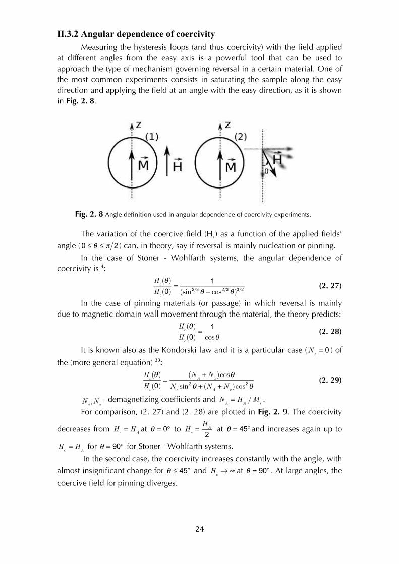
II.3.2 Angular dependence of coercivity

Measuring the hysteresis loops (and thus coercivity) with the field applied

at different angles from the easy axis is a powerful tool that can be used to

approach the type of mechanism governing reversal in a certain material. One of

the most common experiments consists in saturating the sample along the easy

direction and applying the field at an angle with the easy direction, as it is shown

in Fig. 2. 8.

!

Fig. 2. 8 Angle definition used in angular dependence of coercivity experiments.

The variation of the coercive field (Hc) as a function of the applied fields’

angle ( 0 ≤ θ ≤ π 2 ) can, in theory, say if reversal is mainly nucleation or pinning.

In the case of Stoner - Wohlfarth systems, the angular dependence of

coercivity is 4:

!

Hc(θ)

Hc(0)

=1

(sin2/3θ + cos2/3

θ)3/2! (2. 27)

In the case of pinning materials (or passage) in which reversal is mainly

due to magnetic domain wall movement through the material, the theory predicts:

!

Hc(θ)

Hc(0)

=1

cosθ! (2. 28)

It is known also as the Kondorski law and it is a particular case ( N

z= 0 ) of

the (more general equation) 23:

!

Hc(θ)

Hc(0)

=(N

A+N

x)cosθ

Nzsin2

θ + (NA+N

x)cos2

θ! (2. 29)

N

x,N

z

- demagnetizing coefficients and N

A= H

A/M

s.

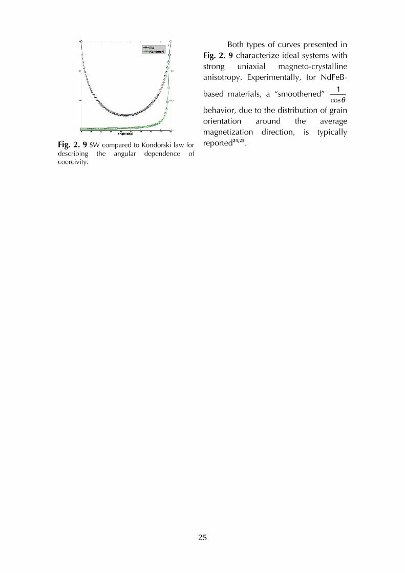
For comparison, (2. 27) and (2. 28) are plotted in Fig. 2. 9. The coercivity

decreases from H

c= H

Aat θ = 0° to

Hc=

HA

2 at θ = 45°and increases again up to

H

c= H

A for θ = 90° for Stoner - Wohlfarth systems.

In the second case, the coercivity increases constantly with the angle, with

almost insignificant change for θ ≤ 45° and H

c→ ∞ at θ = 90° . At large angles, the

coercive field for pinning diverges.

! 25!

Both types of curves presented in

Fig. 2. 9 characterize ideal systems with

strong uniaxial magneto-crystalline

anisotropy. Experimentally, for NdFeB-

based materials, a “smoothened”

1

cosθ

behavior, due to the distribution of grain

orientation around the average

magnetization direction, is typically

reported24,25. !

Fig. 2. 9 SW compared to Kondorski law for describing the angular dependence of coercivity.

! 26!

!

!!!!!!!!!!!!!!!!!!!!!!!!!!!!!!!!!!!!!!!!!!!!!!!!!!!!!!!!

1 G. Bertotti, Hysteresis in Magnetism. For physicists, materials scientists and engineers, Academic Press, 558p (1998);

2 R. Skomski and J.M.D Coey, Permanent magnetism, Taylor & Francis, 420p (1999);

3 P. Bruno, Physical origins and theoretical models of magnetic anisotropy, “Magnetismus von Festkörpern und grenzflächen”, edited by P.H. Dederichs, P. Grünberg and W. Zinn, 24. IFF-Ferienkurs, 24.1-24.8, Forschungszentrum Jülich (1993);

4 E.C.Stoner and E.P. Wohlfarth, Phil. Trans. of the Roy. Soc. Lond. Series A, math. And Phys. Sc. 240, 599 (1948);

5 Y. Ishii, J. Appl. Phys. 70, 3765 (1991);

6 A. Aharoni, Introduction to the Theory of ferromagnetism, Oxford University Press, Oxford, 319p (1996);

7 R. Friedberg and D. I. Paul, Phys. Rev. Lett. 34, 1234 (1975);

8 H.R. Hilzinger and H. Kronmüller, Phys. Lett., 51A, 59 (1975);

9 H. Kronmüller et al., Int. J. Magn. 5, 27 (1973);

10 D. Givord, M. Rossignol and V.M.T.S. Barthem, JMMM 258, 1 (2003);

11 H. Kronmüller and K.D. Durst, JMMM 74, 291 (1988);

12 A. Fukuno, K. Hirose and T. Yoneyama, J. Appl. Phys. 67, 4750 (1990);

13 F. Kools, J. Phys. C6, 349 (1985);

14 S. Hirosawa, K. Tokuhara, Y. Matsuura, H. Yamamoto, S. Fujimura and M. Sagawa, JMMM 61, 363 (1986);

15 H. Kronmuller, K. D. Durst and G. Martinek, JMMM 69, 149 (1987);

16 J. Hu, X.C. Kou and H. Kronmüller, Phys. Stat. Sol. (a) 138, K41 (1993);

17 D.W. Taylor, thesis Lab. Magn. L. Neel, Grenoble (1992);

18 K.D. Durst and H. Kronmüller, JMMM 59, 86 (1986);

19 D. Givord, P. Tenaud and T. Viadieu, IEEE Trans. Magn. 24, 1921 (1988);

20 V.T.M.S Barthem, D. Givord, M. F. Rossignol and P. Tenaud, Physica B 319, 127 (2002);

21 R. Street and J. C. Woolley, Proc. Phys. Soc. 62, 562 (1949);

22 Q. Yao, R. Grössinger, W. Liu, W.B. Cui, F. Yang, X.G. Zhao and Z. D. Zhang, JMMM 324, 2854 (2012);

! 27!

!!!!!!!!!!!!!!!!!!!!!!!!!!!!!!!!!!!!!!!!!!!!!!!!!!!!!!!!

23 R.M. Grechishkin, S. S. Soshin and S. E. Ilyashenko, 1st Int. Workshop on Simulation of Magnetization Processes, SMP95_72 (1995);

24 D. Elbaz, D. Givord, S. Hirosawa, F. P. Missell, M. F. Rossignol and V. Villas-Boas, J. Appl. Phys. 69, 5492 (1991);

25 F. Cebollada, M. F. Rossignol and D. Givord, Phys. Rev. B 52, 13511 (1995).

!

! 28!

III. Sample preparation and characterization techniques

!

Preparation

During this thesis, two types of samples were analyzed:

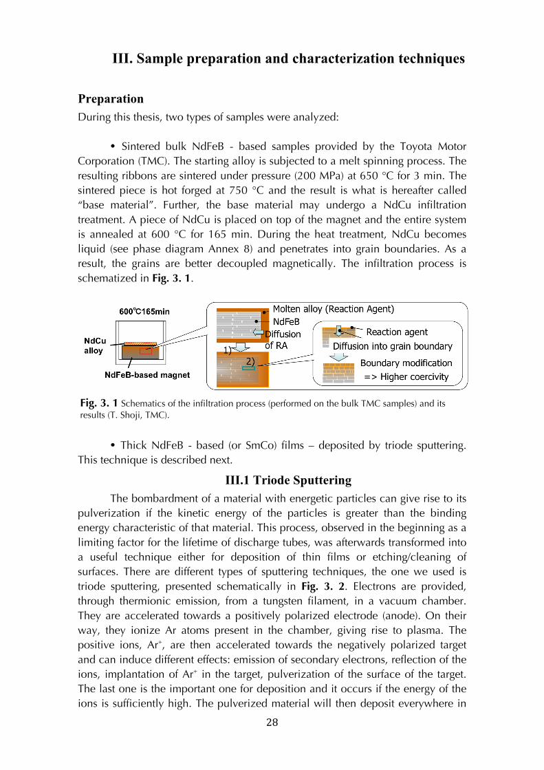
Sintered bulk NdFeB - based samples provided by the Toyota Motor

Corporation (TMC). The starting alloy is subjected to a melt spinning process. The

resulting ribbons are sintered under pressure (200 MPa) at 650 °C for 3 min. The

sintered piece is hot forged at 750 °C and the result is what is hereafter called

“base material”. Further, the base material may undergo a NdCu infiltration

treatment. A piece of NdCu is placed on top of the magnet and the entire system

is annealed at 600 °C for 165 min. During the heat treatment, NdCu becomes

liquid (see phase diagram Annex 8) and penetrates into grain boundaries. As a

result, the grains are better decoupled magnetically. The infiltration process is

schematized in Fig. 3. 1.

Fig. 3. 1 Schematics of the infiltration process (performed on the bulk TMC samples) and its results (T. Shoji, TMC).

Thick NdFeB - based (or SmCo) films – deposited by triode sputtering.

This technique is described next.

III.1 Triode Sputtering

The bombardment of a material with energetic particles can give rise to its

pulverization if the kinetic energy of the particles is greater than the binding

energy characteristic of that material. This process, observed in the beginning as a

limiting factor for the lifetime of discharge tubes, was afterwards transformed into

a useful technique either for deposition of thin films or etching/cleaning of

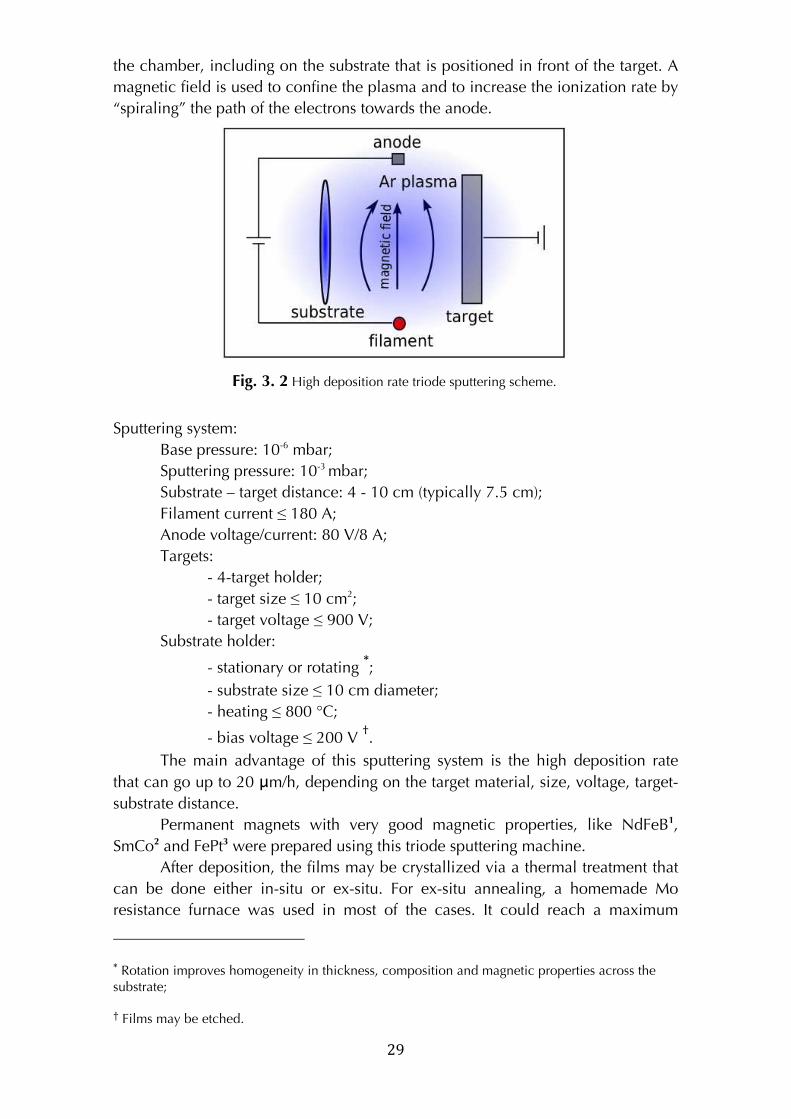
surfaces. There are different types of sputtering techniques, the one we used is

triode sputtering, presented schematically in Fig. 3. 2. Electrons are provided,

through thermionic emission, from a tungsten filament, in a vacuum chamber.

They are accelerated towards a positively polarized electrode (anode). On their

way, they ionize Ar atoms present in the chamber, giving rise to plasma. The

positive ions, Ar+, are then accelerated towards the negatively polarized target

and can induce different effects: emission of secondary electrons, reflection of the

ions, implantation of Ar+ in the target, pulverization of the surface of the target.

The last one is the important one for deposition and it occurs if the energy of the

ions is sufficiently high. The pulverized material will then deposit everywhere in

! 29!

the chamber, including on the substrate that is positioned in front of the target. A

magnetic field is used to confine the plasma and to increase the ionization rate by

“spiraling” the path of the electrons towards the anode.

!

Fig. 3. 2 High deposition rate triode sputtering scheme.

Sputtering system:

Base pressure: 10-6 mbar;

Sputtering pressure: 10-3 mbar;

Substrate – target distance: 4 - 10 cm (typically 7.5 cm);

Filament current ≤ 180 A;

Anode voltage/current: 80 V/8 A;

Targets:

- 4-target holder;

- target size ≤ 10 cm2;

- target voltage ≤ 900 V;

Substrate holder:

- stationary or rotating *;

- substrate size ≤ 10 cm diameter;

- heating ≤ 800 °C;

- bias voltage ≤ 200 V †.

The main advantage of this sputtering system is the high deposition rate

that can go up to 20 μm/h, depending on the target material, size, voltage, target-

substrate distance.

Permanent magnets with very good magnetic properties, like NdFeB1,

SmCo2 and FePt3 were prepared using this triode sputtering machine.

After deposition, the films may be crystallized via a thermal treatment that

can be done either in-situ or ex-situ. For ex-situ annealing, a homemade Mo

resistance furnace was used in most of the cases. It could reach a maximum

!!!!!!!!!!!!!!!!!!!!!!!!!!!!!!!!!!!!!!!!!!!!!!!!!!!!!!!!

*!Rotation improves homogeneity in thickness, composition and magnetic properties across the substrate;!

†!Films may be etched.!

! 30!

temperature of 1200 °C and a maximum ramp rate of around 10 °C/s for samples

≤ 4 cm in diameter. Recently, a Rapid Thermal Annealing (RTA) furnace was

acquired. Substrates of maximum size 10 cm can be annealed, for temperatures

up to 1300 °C and ramp rates between 1 °C/s and 300 °C/s.

Characterization

III.2 Vibrating Sample Magnetometer (VSM)

Magnetic measurements were performed using either VSM or VSM SQUID

magnetometers.

Faraday’s law of induction states that when the magnetic environment of a

coil is changed, there will be a voltage induced in that coil (

V ∝ −ΔΦ

Δt). Many

magnetometers work using this principle. A net magnetic moment is induced in

the sample to be measured by placing it in the magnetic field produced by a

super-conducting coil. The sample is placed in the center of the detection coils,

coils that will measure the voltage induced as a result of the vibration of the

sample in the magnetic field. The measured voltage is proportional to the

magnetization of the sample

( V ∝ −

ΔΦ

Δt⇒ V(t)dt ∝ −

ΔΦ

Δtdt ∝ ΔB ∝ ΔH + ΔM∫∫∫∫∫ ∝ ΔM∫ ). In this expression,

ΔH = 0∫ due to the anti-parallel winding of the detection coils.

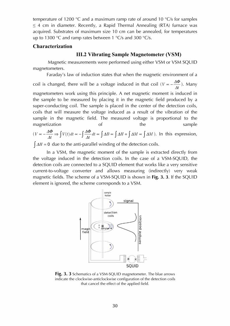
In a VSM, the magnetic moment of the sample is extracted directly from

the voltage induced in the detection coils. In the case of a VSM-SQUID, the

detection coils are connected to a SQUID element that works like a very sensitive

current-to-voltage converter and allows measuring (indirectly) very weak

magnetic fields. The scheme of a VSM-SQUID is shown in Fig. 3. 3. If the SQUID

element is ignored, the scheme corresponds to a VSM.

Fig. 3. 3 Schematics of a VSM-SQUID magnetometer. The blue arrows indicate the clockwise-anticlockwise configuration of the detection coils

that cancel the effect of the applied field.

! 31!

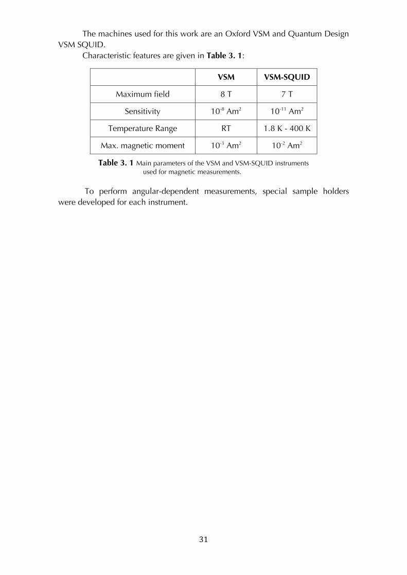
The machines used for this work are an Oxford VSM and Quantum Design

VSM SQUID.

Characteristic features are given in Table 3. 1:

VSM VSM-SQUID

Maximum field 8 T 7 T

Sensitivity 10-8 Am2 10-11 Am2

Temperature Range RT 1.8 K - 400 K

Max. magnetic moment 10-3 Am2 10-2 Am2

Table 3. 1 Main parameters of the VSM and VSM-SQUID instruments used for magnetic measurements. !

To perform angular-dependent measurements, special sample holders

were developed for each instrument.

! 32!

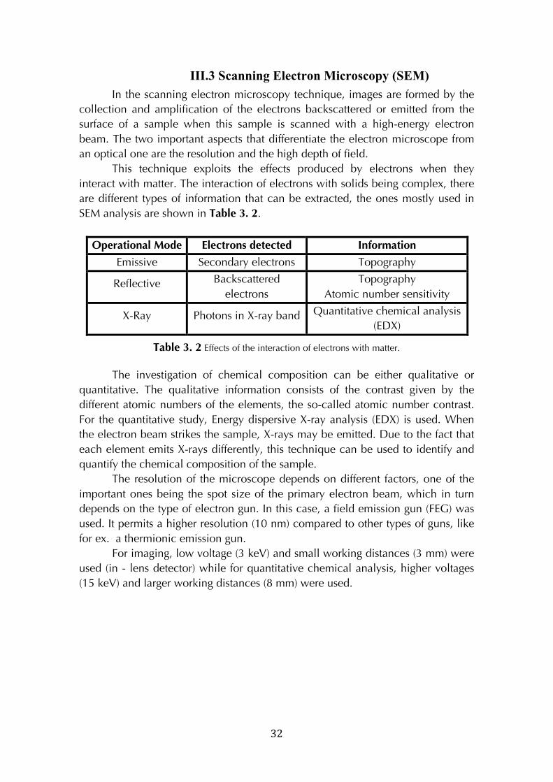
III.3 Scanning Electron Microscopy (SEM)

In the scanning electron microscopy technique, images are formed by the

collection and amplification of the electrons backscattered or emitted from the

surface of a sample when this sample is scanned with a high-energy electron

beam. The two important aspects that differentiate the electron microscope from

an optical one are the resolution and the high depth of field.

This technique exploits the effects produced by electrons when they

interact with matter. The interaction of electrons with solids being complex, there

are different types of information that can be extracted, the ones mostly used in

SEM analysis are shown in Table 3. 2.

Operational Mode Electrons detected Information

Emissive Secondary electrons Topography

Reflective Backscattered

electrons

Topography

Atomic number sensitivity

X-Ray Photons in X-ray band Quantitative chemical analysis

(EDX) !

Table 3. 2 Effects of the interaction of electrons with matter.

The investigation of chemical composition can be either qualitative or

quantitative. The qualitative information consists of the contrast given by the

different atomic numbers of the elements, the so-called atomic number contrast.

For the quantitative study, Energy dispersive X-ray analysis (EDX) is used. When

the electron beam strikes the sample, X-rays may be emitted. Due to the fact that

each element emits X-rays differently, this technique can be used to identify and

quantify the chemical composition of the sample.

The resolution of the microscope depends on different factors, one of the

important ones being the spot size of the primary electron beam, which in turn

depends on the type of electron gun. In this case, a field emission gun (FEG) was

used. It permits a higher resolution (10 nm) compared to other types of guns, like

for ex. a thermionic emission gun.

For imaging, low voltage (3 keV) and small working distances (3 mm) were

used (in - lens detector) while for quantitative chemical analysis, higher voltages

(15 keV) and larger working distances (8 mm) were used.

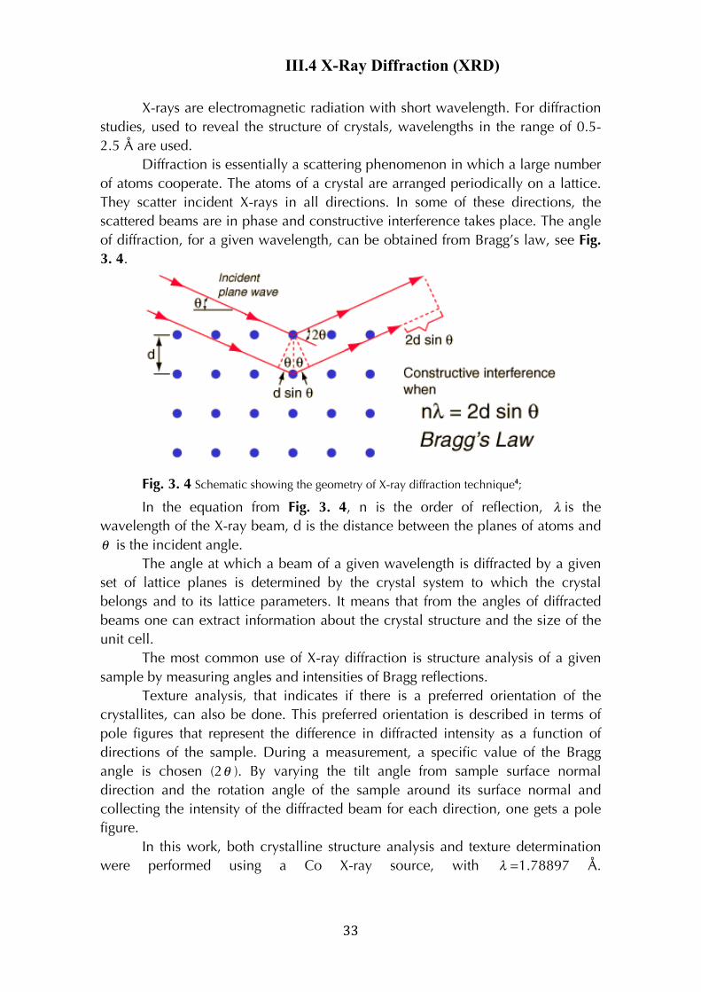
! 33!

III.4 X-Ray Diffraction (XRD)

X-rays are electromagnetic radiation with short wavelength. For diffraction

studies, used to reveal the structure of crystals, wavelengths in the range of 0.5-2.5 Å are used.

Diffraction is essentially a scattering phenomenon in which a large number of atoms cooperate. The atoms of a crystal are arranged periodically on a lattice. They scatter incident X-rays in all directions. In some of these directions, the scattered beams are in phase and constructive interference takes place. The angle of diffraction, for a given wavelength, can be obtained from Bragg’s law, see Fig.

3. 4.

Fig. 3. 4 Schematic showing the geometry of X-ray diffraction technique4;

In the equation from Fig. 3. 4, n is the order of reflection, λ is the wavelength of the X-ray beam, d is the distance between the planes of atoms and θ is the incident angle.

The angle at which a beam of a given wavelength is diffracted by a given set of lattice planes is determined by the crystal system to which the crystal belongs and to its lattice parameters. It means that from the angles of diffracted beams one can extract information about the crystal structure and the size of the unit cell.

The most common use of X-ray diffraction is structure analysis of a given sample by measuring angles and intensities of Bragg reflections.

Texture analysis, that indicates if there is a preferred orientation of the crystallites, can also be done. This preferred orientation is described in terms of pole figures that represent the difference in diffracted intensity as a function of directions of the sample. During a measurement, a specific value of the Bragg angle is chosen (2θ ). By varying the tilt angle from sample surface normal direction and the rotation angle of the sample around its surface normal and collecting the intensity of the diffracted beam for each direction, one gets a pole figure.

In this work, both crystalline structure analysis and texture determination were performed using a Co X-ray source, with λ =1.78897 Å.

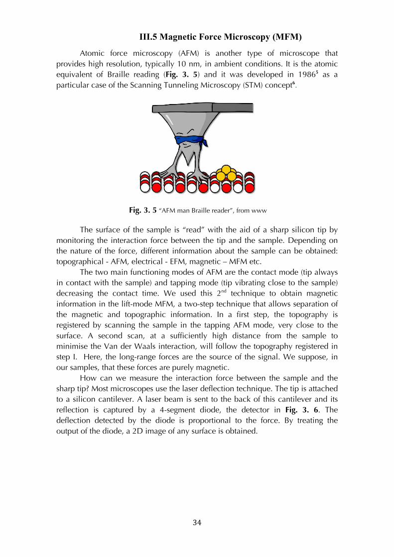
! 34!

III.5 Magnetic Force Microscopy (MFM)

Atomic force microscopy (AFM) is another type of microscope that

provides high resolution, typically 10 nm, in ambient conditions. It is the atomic

equivalent of Braille reading (Fig. 3. 5) and it was developed in 19865 as a

particular case of the Scanning Tunneling Microscopy (STM) concept6.

!

Fig. 3. 5 “AFM man Braille reader”, from www

The surface of the sample is “read” with the aid of a sharp silicon tip by

monitoring the interaction force between the tip and the sample. Depending on

the nature of the force, different information about the sample can be obtained:

topographical - AFM, electrical - EFM, magnetic – MFM etc.

The two main functioning modes of AFM are the contact mode (tip always

in contact with the sample) and tapping mode (tip vibrating close to the sample)

decreasing the contact time. We used this 2nd technique to obtain magnetic

information in the lift-mode MFM, a two-step technique that allows separation of

the magnetic and topographic information. In a first step, the topography is

registered by scanning the sample in the tapping AFM mode, very close to the

surface. A second scan, at a sufficiently high distance from the sample to

minimise the Van der Waals interaction, will follow the topography registered in

step I. Here, the long-range forces are the source of the signal. We suppose, in

our samples, that these forces are purely magnetic.

How can we measure the interaction force between the sample and the

sharp tip? Most microscopes use the laser deflection technique. The tip is attached

to a silicon cantilever. A laser beam is sent to the back of this cantilever and its

reflection is captured by a 4-segment diode, the detector in Fig. 3. 6. The

deflection detected by the diode is proportional to the force. By treating the

output of the diode, a 2D image of any surface is obtained.

!

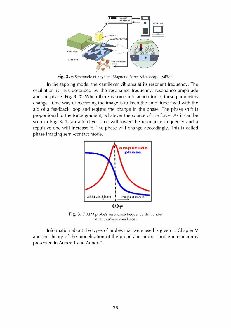
! 35!

!

Fig. 3. 6 Schematic of a typical Magnetic Force Microscope (MFM)7.

In the tapping mode, the cantilever vibrates at its resonant frequency. The

oscillation is thus described by the resonance frequency, resonance amplitude

and the phase, Fig. 3. 7. When there is some interaction force, these parameters

change. One way of recording the image is to keep the amplitude fixed with the

aid of a feedback loop and register the change in the phase. The phase shift is

proportional to the force gradient, whatever the source of the force. As it can be

seen in Fig. 3. 7, an attractive force will lower the resonance frequency and a

repulsive one will increase it. The phase will change accordingly. This is called

phase imaging semi-contact mode.

!

Fig. 3. 7 AFM probe’s resonance frequency shift under attractive/repulsive forces

Information about the types of probes that were used is given in Chapter V

and the theory of the modelisation of the probe and probe-sample interaction is

presented in Annex 1 and Annex 2.

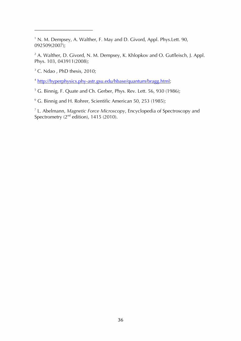
! 36!

!

!!!!!!!!!!!!!!!!!!!!!!!!!!!!!!!!!!!!!!!!!!!!!!!!!!!!!!!!

1 N. M. Dempsey, A. Walther, F. May and D. Givord, Appl. Phys.Lett. 90, 092509(2007);

2 A. Walther, D. Givord, N. M. Dempsey, K. Khlopkov and O. Gutfleisch, J. Appl. Phys. 103, 043911(2008);

3 C. Ndao , PhD thesis, 2010;

4 http://hyperphysics.phy-astr.gsu.edu/hbase/quantum/bragg.html;

5 G. Binnig, F. Quate and Ch. Gerber, Phys. Rev. Lett. 56, 930 (1986);

6 G. Binnig and H. Rohrer, Scientific American 50, 253 (1985);

7 L. Abelmann, Magnetic Force Microscopy, Encyclopedia of Spectroscopy and Spectrometry (2nd edition), 1415 (2010).

!

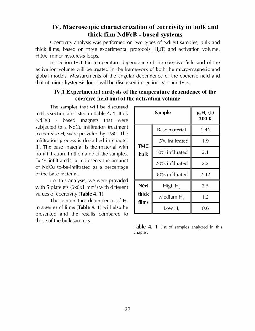
! 37!

IV. Macroscopic characterization of coercivity in bulk and

thick film NdFeB - based systems Coercivity analysis was performed on two types of NdFeB samples, bulk and

thick films, based on three experimental protocols: Hc(T) and activation volume,

Hc(θ), minor hysteresis loops.

In section IV.1 the temperature dependence of the coercive field and of the

activation volume will be treated in the framework of both the micro-magnetic and

global models. Measurements of the angular dependence of the coercive field and

that of minor hysteresis loops will be discussed in section IV.2 and IV.3.

IV.1 Experimental analysis of the temperature dependence of the

coercive field and of the activation volume

The samples that will be discussed

in this section are listed in Table 4. 1. Bulk

NdFeB - based magnets that were

subjected to a NdCu infiltration treatment

to increase Hc were provided by TMC. The

infiltration process is described in chapter

III. The base material is the material with

no infiltration. In the name of the samples,

“x % infiltrated”, x represents the amount

of NdCu to-be-infiltrated as a percentage

of the base material.

For this analysis, we were provided

with 5 platelets (6x6x1 mm3) with different

values of coercivity (Table 4. 1).

The temperature dependence of Hc

in a series of films (Table 4. 1) will also be

presented and the results compared to

those of the bulk samples.

!

!

!

Sample μ0Hc (T) 300 K

Base material 1.46

5% infiltrated 1.9

10% infiltrated 2.1

20% infiltrated 2.2

TMC

bulk

30% infiltrated 2.42

High Hc 2.5

Medium Hc 1.2

Néel

thick

films Low Hc 0.6

Table 4. 1 List of samples analyzed in this chapter.

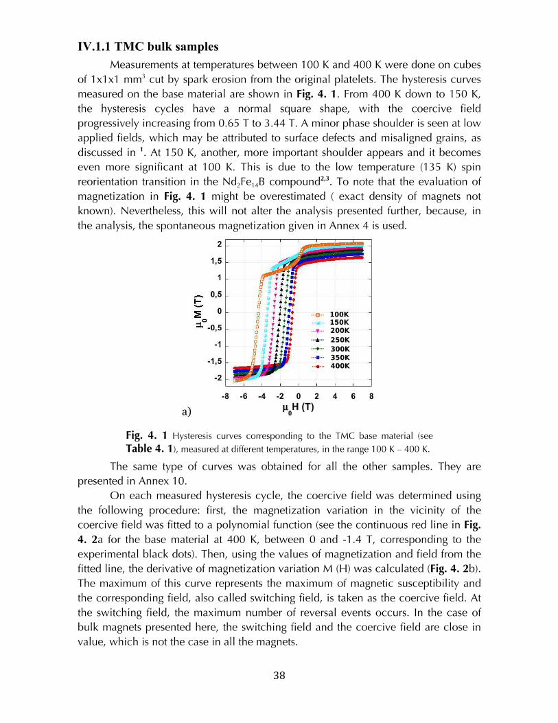
! 38!

IV.1.1 TMC bulk samples

Measurements at temperatures between 100 K and 400 K were done on cubes

of 1x1x1 mm3 cut by spark erosion from the original platelets. The hysteresis curves

measured on the base material are shown in Fig. 4. 1. From 400 K down to 150 K,

the hysteresis cycles have a normal square shape, with the coercive field

progressively increasing from 0.65 T to 3.44 T. A minor phase shoulder is seen at low

applied fields, which may be attributed to surface defects and misaligned grains, as

discussed in 1. At 150 K, another, more important shoulder appears and it becomes

even more significant at 100 K. This is due to the low temperature (135 K) spin

reorientation transition in the Nd2Fe14B compound2,3. To note that the evaluation of

magnetization in Fig. 4. 1 might be overestimated ( exact density of magnets not

known). Nevertheless, this will not alter the analysis presented further, because, in

the analysis, the spontaneous magnetization given in Annex 4 is used.

a)

Fig. 4. 1 Hysteresis curves corresponding to the TMC base material (see

Table 4. 1), measured at different temperatures, in the range 100 K – 400 K.!

The same type of curves was obtained for all the other samples. They are

presented in Annex 10.

On each measured hysteresis cycle, the coercive field was determined using

the following procedure: first, the magnetization variation in the vicinity of the

coercive field was fitted to a polynomial function (see the continuous red line in Fig.

4. 2a for the base material at 400 K, between 0 and -1.4 T, corresponding to the

experimental black dots). Then, using the values of magnetization and field from the

fitted line, the derivative of magnetization variation M (H) was calculated (Fig. 4. 2b).

The maximum of this curve represents the maximum of magnetic susceptibility and

the corresponding field, also called switching field, is taken as the coercive field. At

the switching field, the maximum number of reversal events occurs. In the case of

bulk magnets presented here, the switching field and the coercive field are close in

value, which is not the case in all the magnets.

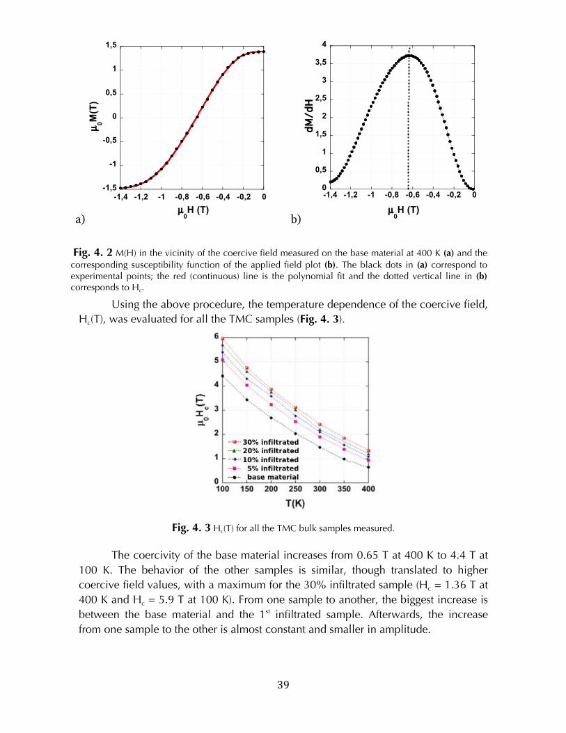
! 39!

a)

-1,5

-1

-0,5

0

0,5

1

1,5

-1,4 -1,2 -1 -0,8 -0,6 -0,4 -0,2 0

µ0M

(T)

µ0H (T)

b)

0

0,5

1

1,5

2

2,5

3

3,5

4

-1,4 -1,2 -1 -0,8 -0,6 -0,4 -0,2 0

dM/dH

µ0H (T)

Fig. 4. 2 M(H) in the vicinity of the coercive field measured on the base material at 400 K (a) and the corresponding susceptibility function of the applied field plot (b). The black dots in (a) correspond to experimental points; the red (continuous) line is the polynomial fit and the dotted vertical line in (b) corresponds to Hc.!

Using the above procedure, the temperature dependence of the coercive field,

Hc(T), was evaluated for all the TMC samples (Fig. 4. 3).

Fig. 4. 3 Hc(T) for all the TMC bulk samples measured.!

The coercivity of the base material increases from 0.65 T at 400 K to 4.4 T at

100 K. The behavior of the other samples is similar, though translated to higher

coercive field values, with a maximum for the 30% infiltrated sample (Hc = 1.36 T at

400 K and Hc = 5.9 T at 100 K). From one sample to another, the biggest increase is

between the base material and the 1st infiltrated sample. Afterwards, the increase

from one sample to the other is almost constant and smaller in amplitude.

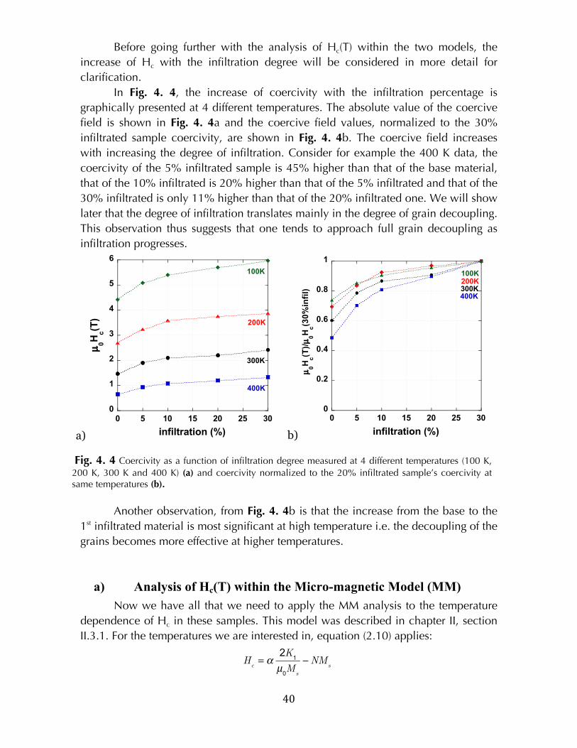
! 40!

Before going further with the analysis of Hc(T) within the two models, the

increase of Hc with the infiltration degree will be considered in more detail for

clarification.

In Fig. 4. 4, the increase of coercivity with the infiltration percentage is

graphically presented at 4 different temperatures. The absolute value of the coercive

field is shown in Fig. 4. 4a and the coercive field values, normalized to the 30%

infiltrated sample coercivity, are shown in Fig. 4. 4b. The coercive field increases

with increasing the degree of infiltration. Consider for example the 400 K data, the

coercivity of the 5% infiltrated sample is 45% higher than that of the base material,

that of the 10% infiltrated is 20% higher than that of the 5% infiltrated and that of the

30% infiltrated is only 11% higher than that of the 20% infiltrated one. We will show

later that the degree of infiltration translates mainly in the degree of grain decoupling.

This observation thus suggests that one tends to approach full grain decoupling as

infiltration progresses.

a)

0

1

2

3

4

5

6

0 5 10 15 20 25 30

µ0H

c(T

)

infiltration (%)

400K

100K

200K

300K

b)

0

0.2

0.4

0.6

0.8

1

0 5 10 15 20 25 30

infiltration (%)

µ0H

c(T

)/µ

0H

c(3

0%

infi

l)

100K200K300K400K

Fig. 4. 4 Coercivity as a function of infiltration degree measured at 4 different temperatures (100 K, 200 K, 300 K and 400 K) (a) and coercivity normalized to the 20% infiltrated sample’s coercivity at same temperatures (b).

Another observation, from Fig. 4. 4b is that the increase from the base to the

1st infiltrated material is most significant at high temperature i.e. the decoupling of the

grains becomes more effective at higher temperatures.

a) Analysis of Hc(T) within the Micro-magnetic Model (MM)

Now we have all that we need to apply the MM analysis to the temperature

dependence of Hc in these samples. This model was described in chapter II, section

II.3.1. For the temperatures we are interested in, equation (2.10) applies:

Hc= α

2K1

µ0M

s

−NMs

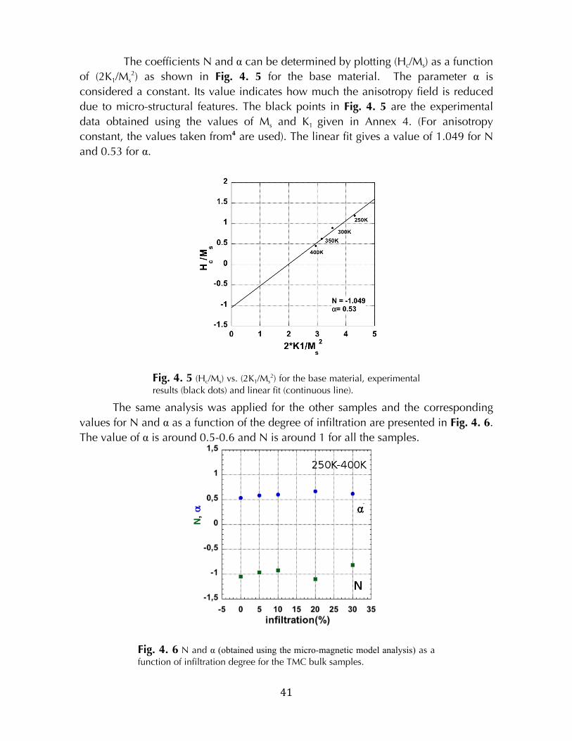
! 41!

The coefficients N and α can be determined by plotting (Hc/Ms) as a function

of (2K1/Ms2) as shown in Fig. 4. 5 for the base material. The parameter α is

considered a constant. Its value indicates how much the anisotropy field is reduced

due to micro-structural features. The black points in Fig. 4. 5 are the experimental

data obtained using the values of Ms and K1 given in Annex 4. (For anisotropy

constant, the values taken from4 are used). The linear fit gives a value of 1.049 for N

and 0.53 for α.

Fig. 4. 5 (Hc/Ms) vs. (2K1/Ms2) for the base material, experimental

results (black dots) and linear fit (continuous line).

The same analysis was applied for the other samples and the corresponding

values for N and α as a function of the degree of infiltration are presented in Fig. 4. 6.

The value of α is around 0.5-0.6 and N is around 1 for all the samples.

Fig. 4. 6 N and α (obtained using the micro-magnetic model analysis) as a function of infiltration degree for the TMC bulk samples.

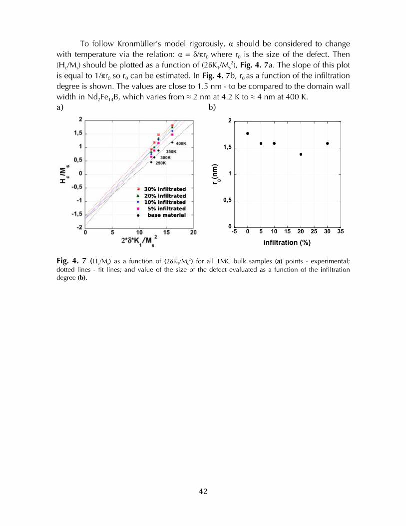
! 42!

To follow Kronmüller’s model rigorously, α should be considered to change

with temperature via the relation: α = δ/πr0 where r0 is the size of the defect. Then

(Hc/Ms) should be plotted as a function of (2δK1/Ms2), Fig. 4. 7a. The slope of this plot

is equal to 1/πr0 so r0 can be estimated. In Fig. 4. 7b, r0 as a function of the infiltration

degree is shown. The values are close to 1.5 nm - to be compared to the domain wall

width in Nd2Fe14B, which varies from ≈ 2 nm at 4.2 K to ≈ 4 nm at 400 K.

a)

b)

0

0,5

1

1,5

2

-5 0 5 10 15 20 25 30 35

r 0(n

m)

infiltration (%)

Fig. 4. 7 (Hc/Ms) as a function of (2δK1/Ms2) for all TMC bulk samples (a) points - experimental;

dotted lines - fit lines; and value of the size of the defect evaluated as a function of the infiltration degree (b)."

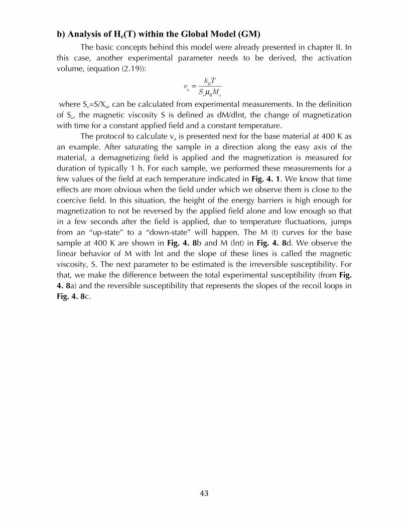
! 43!

b) Analysis of Hc(T) within the Global Model (GM)

The basic concepts behind this model were already presented in chapter II. In

this case, another experimental parameter needs to be derived, the activation

volume, (equation (2.19)):

va=

kBT

Svµ

0M

s

where Sv=S/Xirr can be calculated from experimental measurements. In the definition

of Sv, the magnetic viscosity S is defined as dM/dlnt, the change of magnetization

with time for a constant applied field and a constant temperature.

The protocol to calculate va is presented next for the base material at 400 K as

an example. After saturating the sample in a direction along the easy axis of the

material, a demagnetizing field is applied and the magnetization is measured for

duration of typically 1 h. For each sample, we performed these measurements for a

few values of the field at each temperature indicated in Fig. 4. 1. We know that time

effects are more obvious when the field under which we observe them is close to the

coercive field. In this situation, the height of the energy barriers is high enough for

magnetization to not be reversed by the applied field alone and low enough so that

in a few seconds after the field is applied, due to temperature fluctuations, jumps

from an “up-state” to a “down-state” will happen. The M (t) curves for the base

sample at 400 K are shown in Fig. 4. 8b and M (lnt) in Fig. 4. 8d. We observe the

linear behavior of M with lnt and the slope of these lines is called the magnetic

viscosity, S. The next parameter to be estimated is the irreversible susceptibility. For

that, we make the difference between the total experimental susceptibility (from Fig.

4. 8a) and the reversible susceptibility that represents the slopes of the recoil loops in

Fig. 4. 8c.

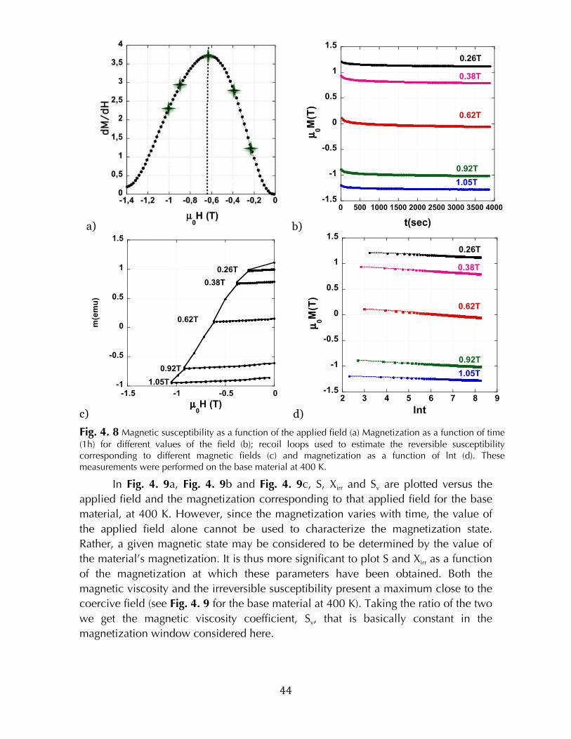
! 44!

a) b)

-1.5

-1

-0.5

0

0.5

1

1.5

0 500 1000 1500 2000 2500 3000 3500 4000

t(sec)

0.26T

0.38T

0.62T

0.92T

1.05T

µ0M(T)

c)

-1

-0.5

0

0.5

1

1.5

-1.5 -1 -0.5 0

m(e

mu

)

µ0H (T)

0.26T

0.38T

0.62T

0.92T

1.05T

d)

-1.5

-1

-0.5

0

0.5

1

1.5

2 3 4 5 6 7 8 9

lnt

0.26T

0.38T

0.62T

0.92T

1.05T

µ0M(T)

Fig. 4. 8 Magnetic susceptibility as a function of the applied field (a) Magnetization as a function of time (1h) for different values of the field (b); recoil loops used to estimate the reversible susceptibility corresponding to different magnetic fields (c) and magnetization as a function of lnt (d). These measurements were performed on the base material at 400 K.

In Fig. 4. 9a, Fig. 4. 9b and Fig. 4. 9c, S, Xirr and Sv are plotted versus the

applied field and the magnetization corresponding to that applied field for the base

material, at 400 K. However, since the magnetization varies with time, the value of

the applied field alone cannot be used to characterize the magnetization state.

Rather, a given magnetic state may be considered to be determined by the value of

the material’s magnetization. It is thus more significant to plot S and Xirr as a function

of the magnetization at which these parameters have been obtained. Both the

magnetic viscosity and the irreversible susceptibility present a maximum close to the

coercive field (see Fig. 4. 9 for the base material at 400 K). Taking the ratio of the two

we get the magnetic viscosity coefficient, Sv, that is basically constant in the

magnetization window considered here.

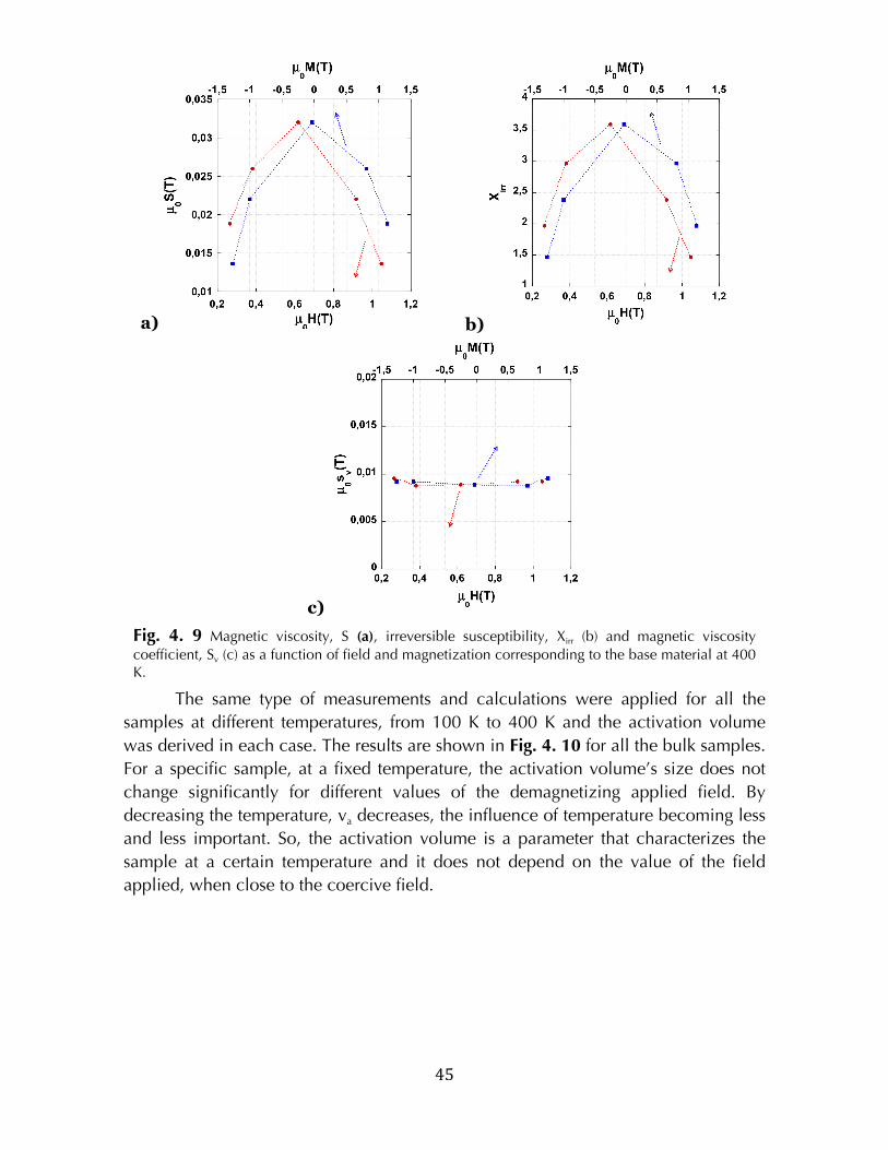
! 45!

a) b)

c)

Fig. 4. 9 Magnetic viscosity, S (a), irreversible susceptibility, Xirr (b) and magnetic viscosity coefficient, Sv (c) as a function of field and magnetization corresponding to the base material at 400 K.

The same type of measurements and calculations were applied for all the

samples at different temperatures, from 100 K to 400 K and the activation volume

was derived in each case. The results are shown in Fig. 4. 10 for all the bulk samples.

For a specific sample, at a fixed temperature, the activation volume’s size does not

change significantly for different values of the demagnetizing applied field. By

decreasing the temperature, va decreases, the influence of temperature becoming less

and less important. So, the activation volume is a parameter that characterizes the

sample at a certain temperature and it does not depend on the value of the field

applied, when close to the coercive field.

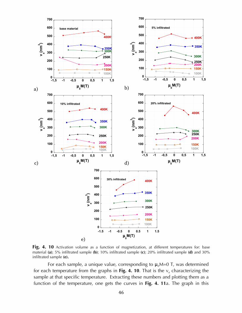
! 46!

a)

0

100

200

300

400

500

600

700

-1,5 -1 -0,5 0 0,5 1 1,5

µ0M(T)

va(n

m3)

400K

350K300K

250K

200K

150K

100K

base material

b)

0

100

200

300

400

500

600

700

-1,5 -1 -0,5 0 0,5 1 1,5

µ0M(T)

va(n

m3)

400K

350K

300K

250K200K

150K

100K

5% infiltrated

c)

0

100

200

300

400

500

600

700

-1,5 -1 -0,5 0 0,5 1 1,5

µ0M(T)

va(n

m3)

400K

350K

300K

250K

200K

150K100K

10% infiltrated

d)

0

100

200

300

400

500

600

700

-1,5 -1 -0,5 0 0,5 1 1,5

µ0M(T)

va(n

m3)

400K

300K250K

200K

150K

100K

20% infiltrated

e)

0

100

200

300

400

500

600

700

-1.5 -1 -0.5 0 0.5 1 1.5

400K

350K

300K

250K

200K

150K

100K

µ0M(T)

va(n

m3)

30% infiltrated

"

Fig. 4. 10 Activation volume as a function of magnetization, at different temperatures for: base material (a); 5% infiltrated sample (b); 10% infiltrated sample (c); 20% infiltrated sample (d) and 30% infiltrated sample (e).

For each sample, a unique value, corresponding to μ0M=0 T, was determined

for each temperature from the graphs in Fig. 4. 10. That is the va characterizing the

sample at that specific temperature. Extracting these numbers and plotting them as a

function of the temperature, one gets the curves in Fig. 4. 11a. The graph in this

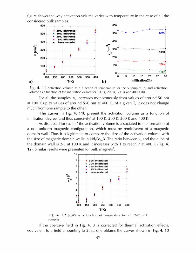
! 47!

figure shows the way activation volume varies with temperature in the case of all the

considered bulk samples.

a) b)

0

100

200

300

400

500

600

0 5 10 15 20 25 30

va(nm

3)

infiltration(%)

400K

300K

200K

100K

Fig. 4. 11 Activation volume as a function of temperature for the 5 samples (a) and activation volume as a function of the infiltration degree for 100 K, 200 K, 300 K and 400 K (b).!

For all the samples, va increases monotonously from values of around 50 nm

at 100 K up to values of around 550 nm at 400 K. At a given T, it does not change

much from one sample to the other.

The curves in Fig. 4. 11b present the activation volume as a function of

infiltration degree (and thus coercivity) at 100 K, 200 K, 300 K and 400 K.

As discussed for ex. in 5 the activation volume is associated to the formation of

a non-uniform magnetic configuration, which must be reminiscent of a magnetic

domain wall. Thus it is legitimate to compare the size of the activation volume with

the size of magnetic domain walls in Nd2Fe14B. The ratio between va and the cube of

the domain wall is 2-3 at 100 K and it increases with T to reach 7 at 400 K (Fig. 4.

12). Similar results were presented for bulk magnets6.

Fig. 4. 12 (va/δ3) as a function of temperature for all TMC bulk

samples.

If the coercive field in Fig. 4. 3 is corrected for thermal activation effects,

equivalent to a field amounting to 25Sv, one obtains the curves shown in Fig. 4. 13

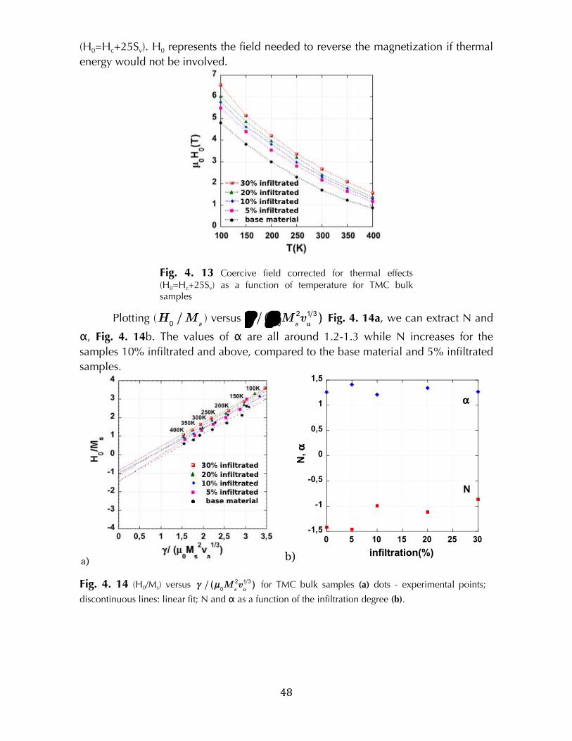
! 48!

(H0=Hc+25Sv). H0 represents the field needed to reverse the magnetization if thermal

energy would not be involved.

Fig. 4. 13 Coercive field corrected for thermal effects (H0=Hc+25Sv) as a function of temperature for TMC bulk samples

Plotting ( H

0/M

s) versus

γ /(µ

0M

s

2v

a

1/3) Fig. 4. 14a, we can extract N and

α, Fig. 4. 14b. The values of α are all around 1.2-1.3 while N increases for the

samples 10% infiltrated and above, compared to the base material and 5% infiltrated

samples.

a) b)

-1,5

-1

-0,5

0

0,5

1

1,5

0 5 10 15 20 25 30

N, α

infiltration(%)

N

α

Fig. 4. 14 (H0/Ms) versus γ /(µ

0M

s

2v

a

1/3) for TMC bulk samples (a) dots - experimental points;

discontinuous lines: linear fit; N and α as a function of the infiltration degree (b). !

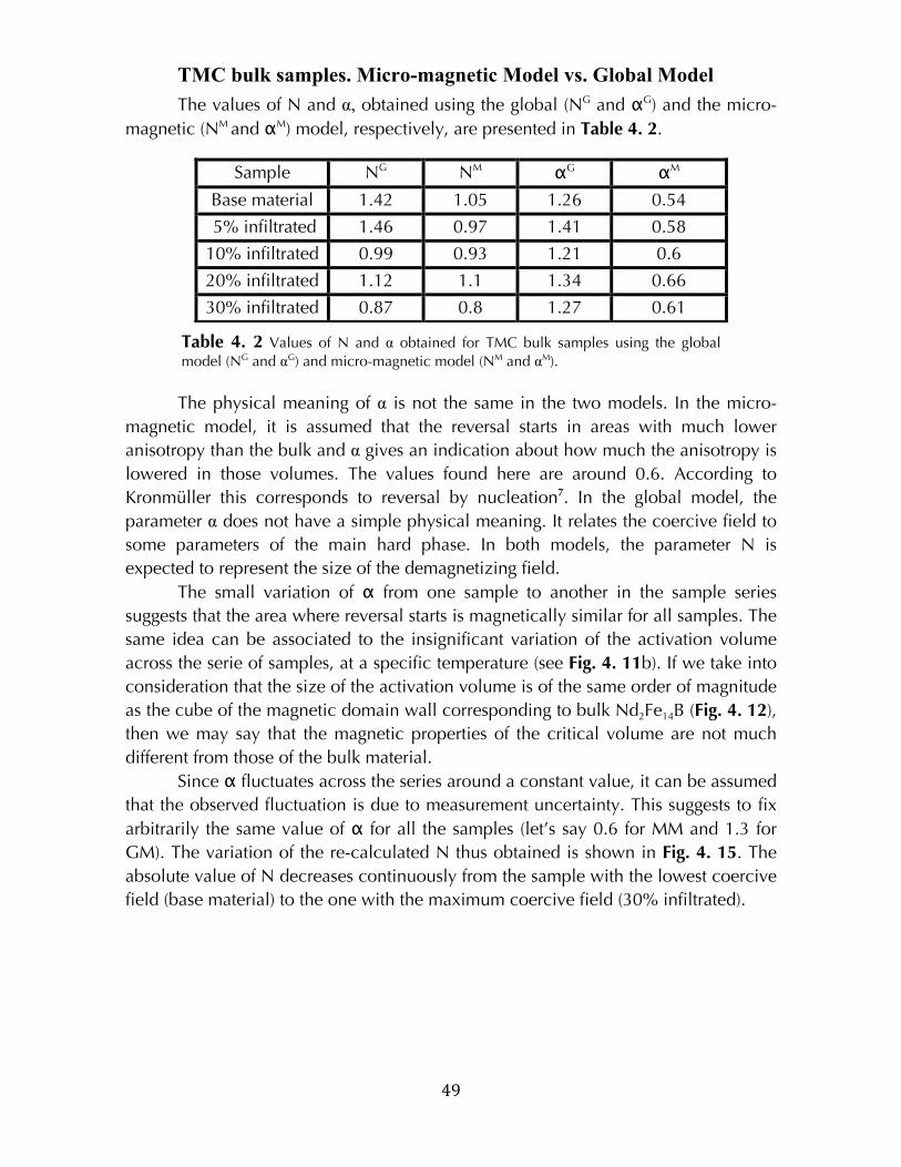
! 49!

TMC bulk samples. Micro-magnetic Model vs. Global Model

The values of N and α, obtained using the global (NG and αG) and the micro-

magnetic (NM and αM) model, respectively, are presented in Table 4. 2.

Sample NG NM αG α

M

Base material 1.42 1.05 1.26 0.54

5% infiltrated 1.46 0.97 1.41 0.58

10% infiltrated 0.99 0.93 1.21 0.6

20% infiltrated 1.12 1.1 1.34 0.66

30% infiltrated 0.87 0.8 1.27 0.61

Table 4. 2 Values of N and α obtained for TMC bulk samples using the global model (NG and αG) and micro-magnetic model (NM and αM).

The physical meaning of α is not the same in the two models. In the micro-

magnetic model, it is assumed that the reversal starts in areas with much lower

anisotropy than the bulk and α gives an indication about how much the anisotropy is

lowered in those volumes. The values found here are around 0.6. According to

Kronmüller this corresponds to reversal by nucleation7. In the global model, the

parameter α does not have a simple physical meaning. It relates the coercive field to

some parameters of the main hard phase. In both models, the parameter N is

expected to represent the size of the demagnetizing field.

The small variation of α from one sample to another in the sample series

suggests that the area where reversal starts is magnetically similar for all samples. The

same idea can be associated to the insignificant variation of the activation volume

across the serie of samples, at a specific temperature (see Fig. 4. 11b). If we take into

consideration that the size of the activation volume is of the same order of magnitude

as the cube of the magnetic domain wall corresponding to bulk Nd2Fe14B (Fig. 4. 12),

then we may say that the magnetic properties of the critical volume are not much

different from those of the bulk material.

Since α fluctuates across the series around a constant value, it can be assumed

that the observed fluctuation is due to measurement uncertainty. This suggests to fix

arbitrarily the same value of α for all the samples (let’s say 0.6 for MM and 1.3 for

GM). The variation of the re-calculated N thus obtained is shown in Fig. 4. 15. The

absolute value of N decreases continuously from the sample with the lowest coercive

field (base material) to the one with the maximum coercive field (30% infiltrated).

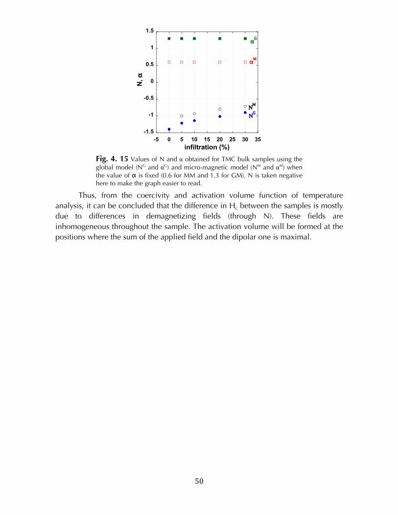
! 50!

-1.5

-1

-0.5

0

0.5

1

1.5

-5 0 5 10 15 20 25 30 35N

, α

infiltration (%)

αG

αM

ΝG

ΝM

Fig. 4. 15 Values of N and α obtained for TMC bulk samples using the global model (NG and αG) and micro-magnetic model (NM and αM) when the value of α is fixed (0.6 for MM and 1.3 for GM). N is taken negative here to make the graph easier to read.

Thus, from the coercivity and activation volume function of temperature

analysis, it can be concluded that the difference in Hc between the samples is mostly

due to differences in demagnetizing fields (through N). These fields are

inhomogeneous throughout the sample. The activation volume will be formed at the

positions where the sum of the applied field and the dipolar one is maximal.

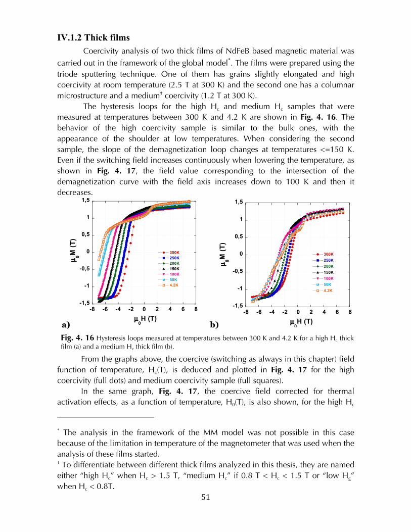
! 51!

IV.1.2 Thick films

Coercivity analysis of two thick films of NdFeB based magnetic material was

carried out in the framework of the global model*. The films were prepared using the

triode sputtering technique. One of them has grains slightly elongated and high

coercivity at room temperature (2.5 T at 300 K) and the second one has a columnar

microstructure and a medium† coercivity (1.2 T at 300 K).

The hysteresis loops for the high Hc and medium Hc samples that were

measured at temperatures between 300 K and 4.2 K are shown in Fig. 4. 16. The

behavior of the high coercivity sample is similar to the bulk ones, with the

appearance of the shoulder at low temperatures. When considering the second

sample, the slope of the demagnetization loop changes at temperatures <=150 K.

Even if the switching field increases continuously when lowering the temperature, as

shown in Fig. 4. 17, the field value corresponding to the intersection of the

demagnetization curve with the field axis increases down to 100 K and then it

decreases.

a)

-1,5

-1

-0,5

0

0,5

1

1,5

-8 -6 -4 -2 0 2 4 6 8

300K

250K

200K

150K

100K

50K

4.2K

µ0M

(T

)

µ0H (T)

b)

-1,5

-1

-0,5

0

0,5

1

1,5

-8 -6 -4 -2 0 2 4 6 8

300K

250K

200K

150K

100K

50K

4.2K

µ0M

(T

)

µ0H (T)

Fig. 4. 16 Hysteresis loops measured at temperatures between 300 K and 4.2 K for a high Hc thick film (a) and a medium Hc thick film (b). !

From the graphs above, the coercive (switching as always in this chapter) field

function of temperature, Hc(T), is deduced and plotted in Fig. 4. 17 for the high

coercivity (full dots) and medium coercivity sample (full squares).

In the same graph, Fig. 4. 17, the coercive field corrected for thermal

activation effects, as a function of temperature, H0(T), is also shown, for the high Hc

!!!!!!!!!!!!!!!!!!!!!!!!!!!!!!!!!!!!!!!!!!!!!!!!!!!!!!!!

* The analysis in the framework of the MM model was not possible in this case

because of the limitation in temperature of the magnetometer that was used when the

analysis of these films started. † To differentiate between different thick films analyzed in this thesis, they are named

either “high Hc” when Hc > 1.5 T, “medium Hc” if 0.8 T < Hc < 1.5 T or “low Hc”

when Hc < 0.8T.

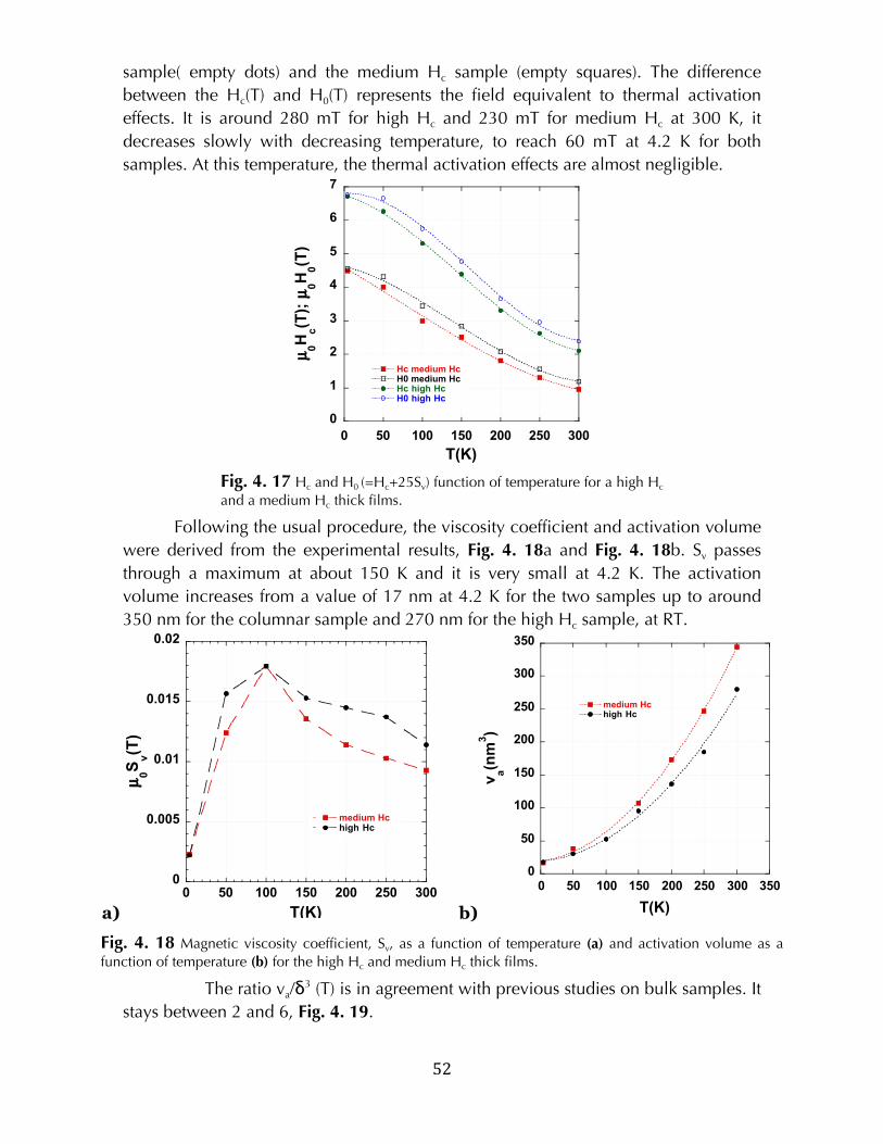
! 52!

sample( empty dots) and the medium Hc sample (empty squares). The difference

between the Hc(T) and H0(T) represents the field equivalent to thermal activation

effects. It is around 280 mT for high Hc and 230 mT for medium Hc at 300 K, it

decreases slowly with decreasing temperature, to reach 60 mT at 4.2 K for both

samples. At this temperature, the thermal activation effects are almost negligible.

0

1

2

3

4

5

6

7

0 50 100 150 200 250 300

Hc medium HcH0 medium HcHc high HcH0 high Hc

µ0H

c(T

); µ

0H

0(T

)

T(K)

Fig. 4. 17 Hc and H0 (=Hc+25Sv) function of temperature for a high Hc and a medium Hc thick films.

Following the usual procedure, the viscosity coefficient and activation volume

were derived from the experimental results, Fig. 4. 18a and Fig. 4. 18b. Sv passes

through a maximum at about 150 K and it is very small at 4.2 K. The activation

volume increases from a value of 17 nm at 4.2 K for the two samples up to around

350 nm for the columnar sample and 270 nm for the high Hc sample, at RT.

a)

0

0.005

0.01

0.015

0.02

0 50 100 150 200 250 300

medium Hchigh Hc

µ0S

v(T

)

T(K) b)

0

50

100

150

200

250

300

350

0 50 100 150 200 250 300 350

medium Hchigh Hc

va(n

m3)

T(K)

Fig. 4. 18 Magnetic viscosity coefficient, Sv, as a function of temperature (a) and activation volume as a function of temperature (b) for the high Hc and medium Hc thick films.

The ratio va/δ3 (T) is in agreement with previous studies on bulk samples. It

stays between 2 and 6, Fig. 4. 19.

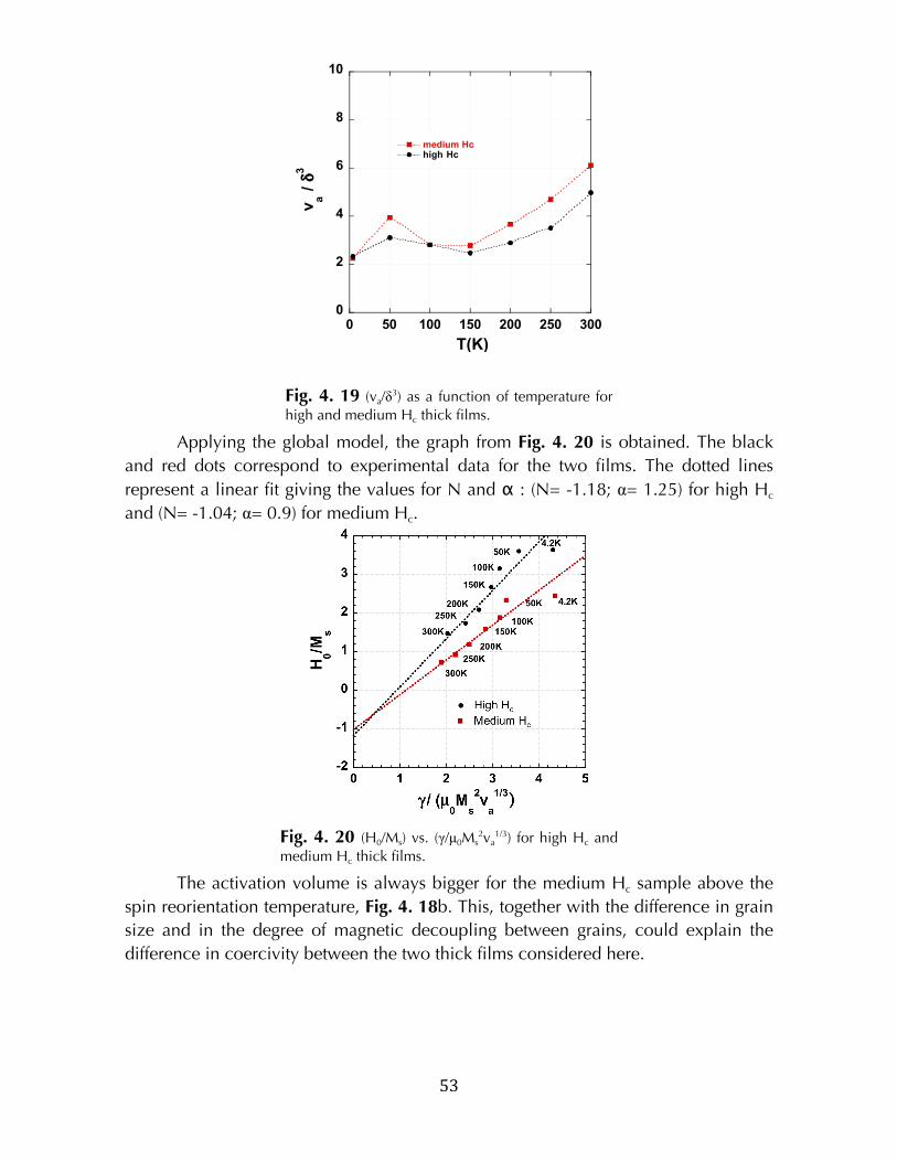
! 53!

0

2

4

6

8

10

0 50 100 150 200 250 300

medium Hchigh Hc

va /

δ3

T(K)

Fig. 4. 19 (va/δ3) as a function of temperature for

high and medium Hc thick films.

Applying the global model, the graph from Fig. 4. 20 is obtained. The black

and red dots correspond to experimental data for the two films. The dotted lines

represent a linear fit giving the values for N and α : (N= -1.18; α= 1.25) for high Hc

and (N= -1.04; α= 0.9) for medium Hc.

Fig. 4. 20 (H0/Ms) vs. (γ/µ0Ms2va

1/3) for high Hc and medium Hc thick films.

The activation volume is always bigger for the medium Hc sample above the

spin reorientation temperature, Fig. 4. 18b. This, together with the difference in grain

size and in the degree of magnetic decoupling between grains, could explain the

difference in coercivity between the two thick films considered here.

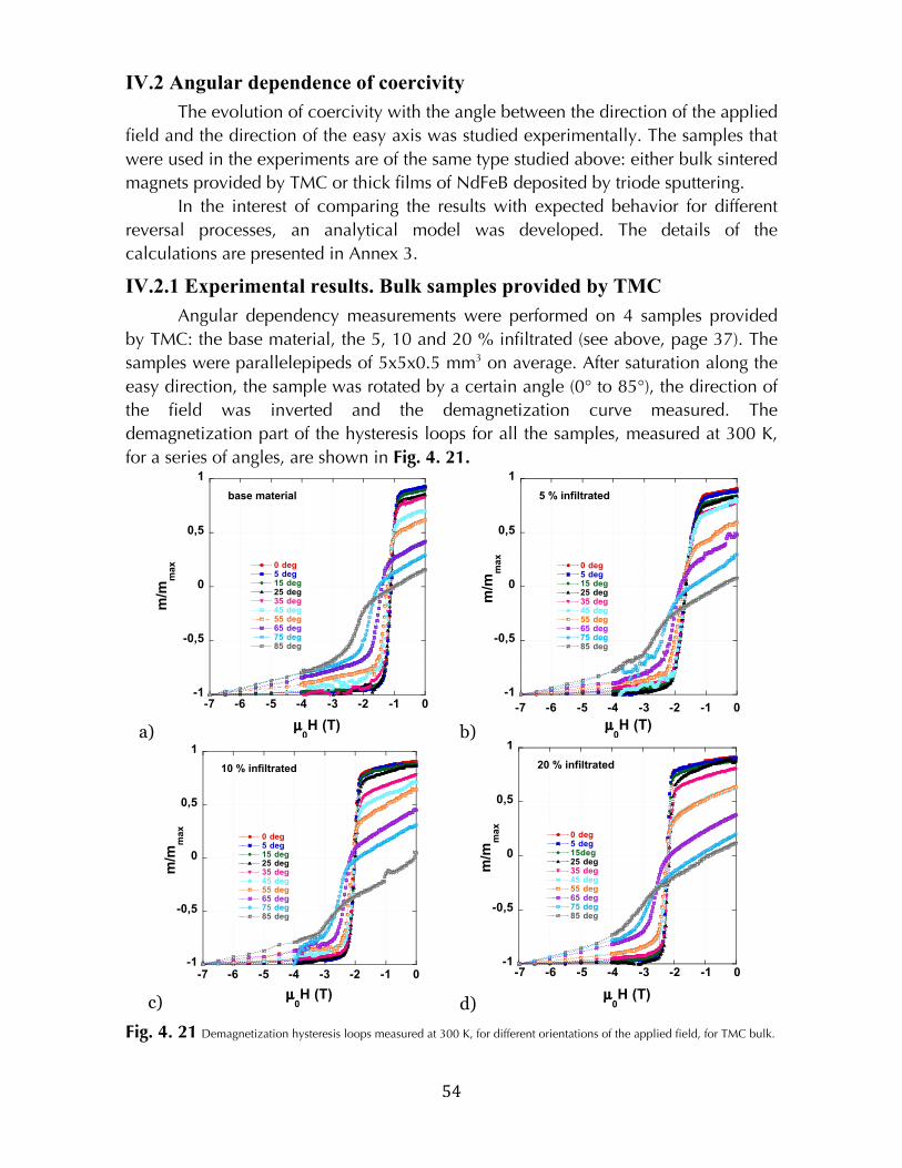
! 54!

IV.2 Angular dependence of coercivity

The evolution of coercivity with the angle between the direction of the applied

field and the direction of the easy axis was studied experimentally. The samples that

were used in the experiments are of the same type studied above: either bulk sintered

magnets provided by TMC or thick films of NdFeB deposited by triode sputtering.

In the interest of comparing the results with expected behavior for different

reversal processes, an analytical model was developed. The details of the

calculations are presented in Annex 3.

IV.2.1 Experimental results. Bulk samples provided by TMC

Angular dependency measurements were performed on 4 samples provided

by TMC: the base material, the 5, 10 and 20 % infiltrated (see above, page 37). The

samples were parallelepipeds of 5x5x0.5 mm3 on average. After saturation along the

easy direction, the sample was rotated by a certain angle (0° to 85°), the direction of

the field was inverted and the demagnetization curve measured. The

demagnetization part of the hysteresis loops for all the samples, measured at 300 K,

for a series of angles, are shown in Fig. 4. 21.

a)

-1

-0,5

0

0,5

1

-7 -6 -5 -4 -3 -2 -1 0

0 deg5 deg15 deg25 deg35 deg45 deg55 deg65 deg75 deg85 deg

m/m

ma

x

µ0H (T)

base material

b)

-1

-0,5

0

0,5

1

-7 -6 -5 -4 -3 -2 -1 0

0 deg5 deg15 deg25 deg35 deg45 deg55 deg65 deg75 deg85 deg

m/m

ma

x

µ0H (T)

5 % infiltrated

c)

-1

-0,5

0

0,5

1

-7 -6 -5 -4 -3 -2 -1 0

0 deg5 deg15 deg25 deg35 deg45 deg55 deg65 deg75 deg85 deg

m/m

ma

x

µ0H (T)

10 % infiltrated

d)

-1

-0,5

0

0,5

1

-7 -6 -5 -4 -3 -2 -1 0

0 deg5 deg15deg25 deg35 deg45 deg55 deg65 deg75 deg85 deg

20 % infiltrated

µ0H (T)

m/m

ma

x

Fig. 4. 21 Demagnetization hysteresis loops measured at 300 K, for different orientations of the applied field, for TMC bulk. !

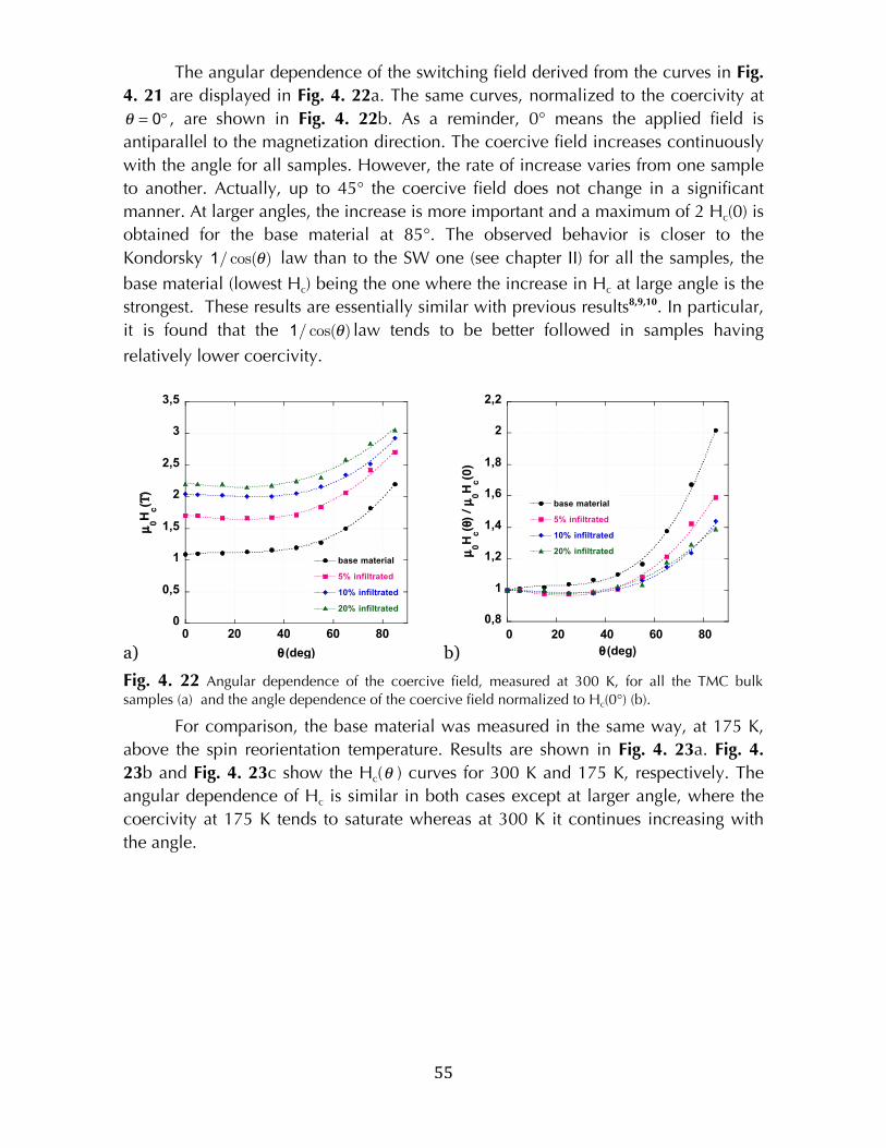
! 55!

The angular dependence of the switching field derived from the curves in Fig.

4. 21 are displayed in Fig. 4. 22a. The same curves, normalized to the coercivity at

θ = 0° , are shown in Fig. 4. 22b. As a reminder, 0° means the applied field is

antiparallel to the magnetization direction. The coercive field increases continuously

with the angle for all samples. However, the rate of increase varies from one sample

to another. Actually, up to 45° the coercive field does not change in a significant

manner. At larger angles, the increase is more important and a maximum of 2 Hc(0) is

obtained for the base material at 85°. The observed behavior is closer to the

Kondorsky 1/ cos(θ) law than to the SW one (see chapter II) for all the samples, the

base material (lowest Hc) being the one where the increase in Hc at large angle is the

strongest. These results are essentially similar with previous results8,9,10. In particular,

it is found that the 1/ cos(θ) law tends to be better followed in samples having

relatively lower coercivity.

a)

0

0,5

1

1,5

2

2,5

3

3,5

0 20 40 60 80

base material

5% infiltrated

10% infiltrated

20% infiltrated

µ0Hc(Τ)

θ (deg) b)

0,8

1

1,2

1,4

1,6

1,8

2

2,2

0 20 40 60 80

base material

5% infiltrated

10% infiltrated

20% infiltratedµ0H

c(θ

) /

µ0H

c(0

)

θ (deg)

Fig. 4. 22 Angular dependence of the coercive field, measured at 300 K, for all the TMC bulk samples (a) and the angle dependence of the coercive field normalized to Hc(0°) (b).

For comparison, the base material was measured in the same way, at 175 K,

above the spin reorientation temperature. Results are shown in Fig. 4. 23a. Fig. 4.

23b and Fig. 4. 23c show the Hc(θ ) curves for 300 K and 175 K, respectively. The

angular dependence of Hc is similar in both cases except at larger angle, where the

coercivity at 175 K tends to saturate whereas at 300 K it continues increasing with

the angle.

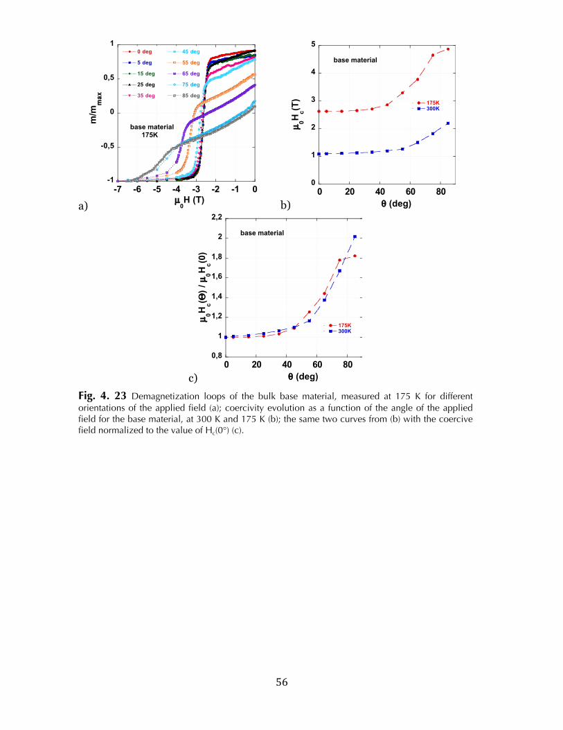
! 56!

a)

-1

-0,5

0

0,5

1

-7 -6 -5 -4 -3 -2 -1 0

0 deg

5 deg

15 deg

25 deg

35 deg

45 deg

55 deg

65 deg

75 deg

85 degm

/mmax

µ0H (T)

base material 175K

b)

0

1

2

3

4

5

0 20 40 60 80

175K300K

µ0H

c(T

)

θ (deg)

base material

c)

0,8

1

1,2

1,4

1,6

1,8

2

2,2

0 20 40 60 80

175K300K

µ0H

c(Θ

) / µ

0H

c(0

)

θ (deg)

base material

Fig. 4. 23 Demagnetization loops of the bulk base material, measured at 175 K for different orientations of the applied field (a); coercivity evolution as a function of the angle of the applied field for the base material, at 300 K and 175 K (b); the same two curves from (b) with the coercive field normalized to the value of Hc(0°) (c).

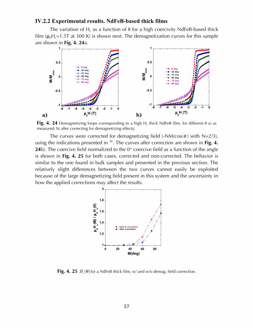
! 57!

IV.2.2 Experimental results. NdFeB-based thick films

The variation of Hc as a function of θ for a high coercivity NdFeB-based thick

film (μ0Hc=1.5T at 300 K) is shown next. The demagnetization curves for this sample

are shown in Fig. 4. 24a.

a)!

-1

-0.5

0

0.5

1

-8 -7 -6 -5 -4 -3 -2 -1 0

0 deg

30 deg

45 deg

60 deg

75 deg

90 degM/M

ma

x

µ0H (T) b)

-1

-0.5

0

0.5

1

-8 -7 -6 -5 -4 -3 -2 -1 0

0 deg

30 deg

45 deg

60 deg

75 deg

90 deg

M/M

max

µ0H (T)

Fig. 4. 24 Demagnetizing loops corresponding to a high Hc thick NdFeB film, for different θ a) as measured; b) after correcting for demagnetizing effects; "

The curves were corrected for demagnetizing field (-NM/cos(θ ) with N=2/3),

using the indications presented in 11. The curves after correction are shown in Fig. 4.

24b). The coercive field normalized to the 0° coercive field as a function of the angle

is shown in Fig. 4. 25 for both cases, corrected and non-corrected. The behavior is

similar to the one found in bulk samples and presented in the previous section. The

relatively slight differences between the two curves cannot easily be exploited

because of the large demagnetizing field present in this system and the uncertainty in

how the applied corrections may affect the results.

1

1,2

1,4

1,6

1,8

2

0 20 40 60 80

before correctionafter correction

µ0H

c(Θ

) / µ

0H

c(0

)

Θ(deg)

Fig. 4. 25 H

c(θ) for a NdFeB thick film, w/ and w/o demag. field correction.

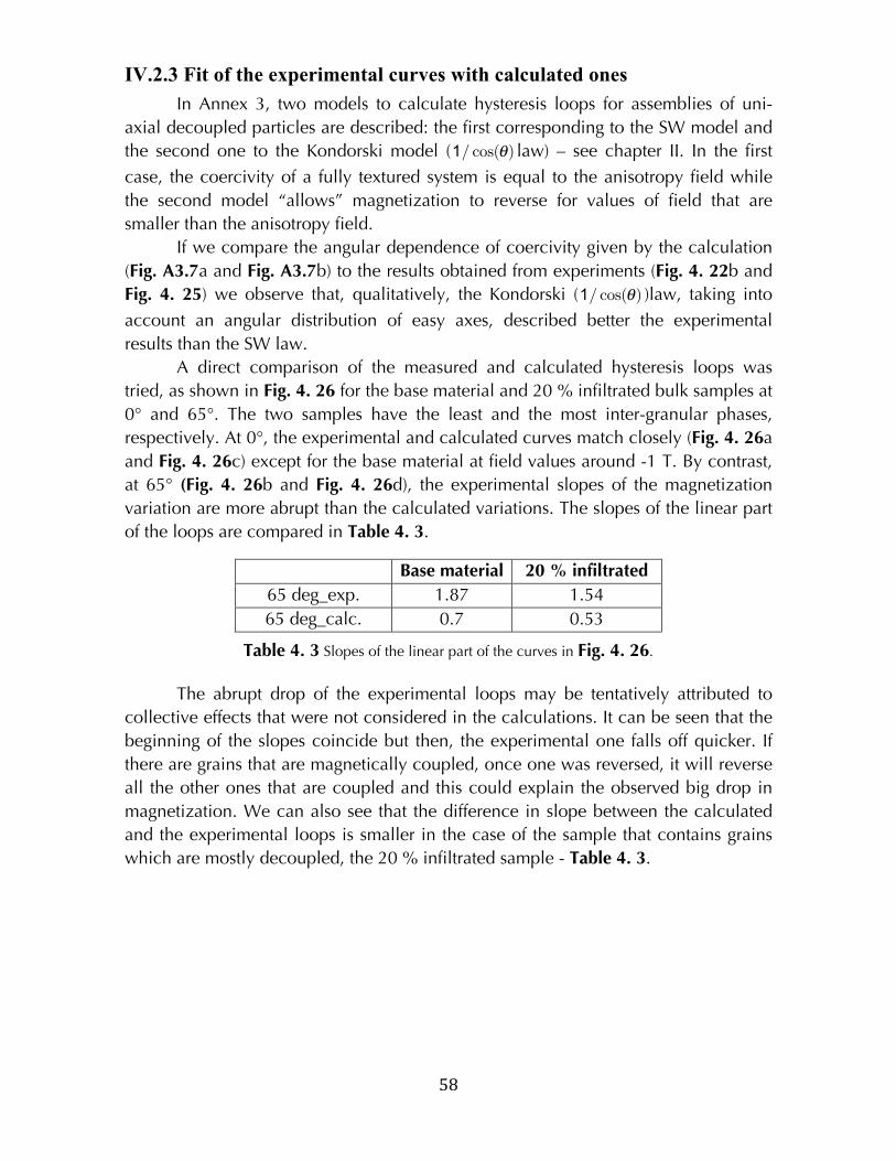
! 58!

IV.2.3 Fit of the experimental curves with calculated ones

In Annex 3, two models to calculate hysteresis loops for assemblies of uni-

axial decoupled particles are described: the first corresponding to the SW model and

the second one to the Kondorski model ( 1/ cos(θ) law) – see chapter II. In the first

case, the coercivity of a fully textured system is equal to the anisotropy field while

the second model “allows” magnetization to reverse for values of field that are

smaller than the anisotropy field.

If we compare the angular dependence of coercivity given by the calculation

(Fig. A3.7a and Fig. A3.7b) to the results obtained from experiments (Fig. 4. 22b and

Fig. 4. 25) we observe that, qualitatively, the Kondorski ( 1/ cos(θ) )law, taking into

account an angular distribution of easy axes, described better the experimental

results than the SW law.

A direct comparison of the measured and calculated hysteresis loops was

tried, as shown in Fig. 4. 26 for the base material and 20 % infiltrated bulk samples at

0° and 65°. The two samples have the least and the most inter-granular phases,

respectively. At 0°, the experimental and calculated curves match closely (Fig. 4. 26a

and Fig. 4. 26c) except for the base material at field values around -1 T. By contrast,

at 65° (Fig. 4. 26b and Fig. 4. 26d), the experimental slopes of the magnetization

variation are more abrupt than the calculated variations. The slopes of the linear part

of the loops are compared in Table 4. 3.

Base material 20 % infiltrated

65 deg_exp. 1.87 1.54

65 deg_calc. 0.7 0.53

Table 4. 3 Slopes of the linear part of the curves in Fig. 4. 26.

The abrupt drop of the experimental loops may be tentatively attributed to

collective effects that were not considered in the calculations. It can be seen that the

beginning of the slopes coincide but then, the experimental one falls off quicker. If

there are grains that are magnetically coupled, once one was reversed, it will reverse

all the other ones that are coupled and this could explain the observed big drop in

magnetization. We can also see that the difference in slope between the calculated

and the experimental loops is smaller in the case of the sample that contains grains

which are mostly decoupled, the 20 % infiltrated sample - Table 4. 3.

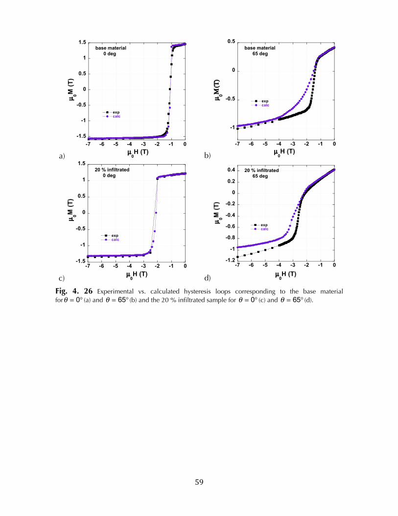
! 59!

a)

-1.5

-1

-0.5

0

0.5

1

1.5

-7 -6 -5 -4 -3 -2 -1 0

expcalc

µ0M

(T

)

µ0H (T)

base material 0 deg

b)

-1

-0.5

0

0.5

-7 -6 -5 -4 -3 -2 -1 0

expcalc

µ0Μ

(Τ

)

µ0H (T)

base material 65 deg

c)

-1.5

-1

-0.5

0

0.5

1

1.5

-7 -6 -5 -4 -3 -2 -1 0

expcalc

µ0M

(T

)

µ0H (T)

20 % infiltrated 0 deg

d)

-1.2

-1

-0.8

-0.6

-0.4

-0.2

0

0.2

0.4

-7 -6 -5 -4 -3 -2 -1 0

expcalc

µ0M

(T

)

µ0H (T)

20 % infiltrated 65 deg

Fig. 4. 26 Experimental vs. calculated hysteresis loops corresponding to the base material

for θ = 0° (a) and θ = 65° (b) and the 20 % infiltrated sample for θ = 0° (c) and θ = 65° (d).

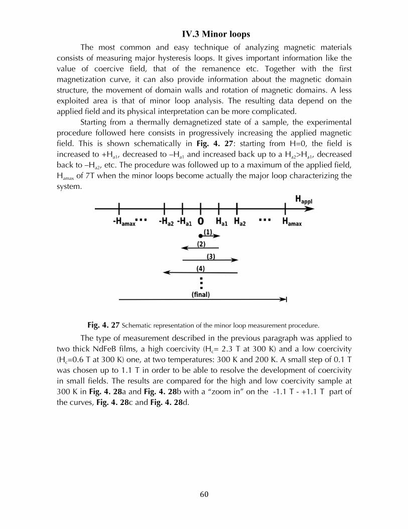
! 60!

IV.3 Minor loops

The most common and easy technique of analyzing magnetic materials

consists of measuring major hysteresis loops. It gives important information like the

value of coercive field, that of the remanence etc. Together with the first

magnetization curve, it can also provide information about the magnetic domain

structure, the movement of domain walls and rotation of magnetic domains. A less

exploited area is that of minor loop analysis. The resulting data depend on the

applied field and its physical interpretation can be more complicated.

Starting from a thermally demagnetized state of a sample, the experimental

procedure followed here consists in progressively increasing the applied magnetic

field. This is shown schematically in Fig. 4. 27: starting from H=0, the field is

increased to +Ha1, decreased to –Ha1 and increased back up to a Ha2>Ha1, decreased

back to –Ha2, etc. The procedure was followed up to a maximum of the applied field,

Hamax of 7T when the minor loops become actually the major loop characterizing the

system.

Fig. 4. 27 Schematic representation of the minor loop measurement procedure.!

The type of measurement described in the previous paragraph was applied to

two thick NdFeB films, a high coercivity (Hc= 2.3 T at 300 K) and a low coercivity

(Hc=0.6 T at 300 K) one, at two temperatures: 300 K and 200 K. A small step of 0.1 T

was chosen up to 1.1 T in order to be able to resolve the development of coercivity

in small fields. The results are compared for the high and low coercivity sample at

300 K in Fig. 4. 28a and Fig. 4. 28b with a “zoom in” on the -1.1 T - +1.1 T part of

the curves, Fig. 4. 28c and Fig. 4. 28d.

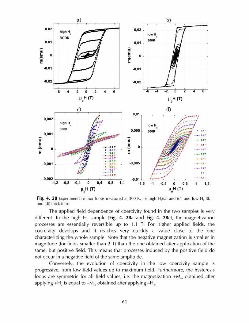
! 61!

a)

-0.02

-0.01

0

0.01

0.02

-6 -4 -2 0 2 4 6

m(e

mu

)

µ0H (T)

high Hc

300K

b)

-0,02

-0,01

0

0,01

0,02

-6 -4 -2 0 2 4 6

m(e

mu

)

µ0H (T)

low Hc

300K

c)

-0,002

-0,001

0

0,001

0,002

-1,2 -0,8 -0,4 0 0,4 0,8 1,2

0.1 T0.2 T0.3 T0.4 T0.5 T0.6 T0.7 T0.8 T0.9 T1 T1.1 T

m (

em

u)

µ0H (T)

high Hc

300K

d)

-0,01

-0,005

0

0,005

0,01

-1,5 -1 -0,5 0 0,5 1 1,5

0.1 T

0.2 T

0.3 T

0.4 T

0.5 T

0.6 T

0.7 T

0.8 T

0.9 T

1 T

1.1 T

m (

em

u)

µ0H (T)

low Hc

300K

Fig. 4. 28 Experimental minor loops measured at 300 K, for high Hc((a) and (c)) and low Hc ((b) and (d)) thick films."

The applied field dependence of coercivity found in the two samples is very

different. In the high Hc sample (Fig. 4. 28a and Fig. 4. 28c), the magnetization

processes are essentially reversible up to 1.1 T. For higher applied fields, the

coercivity develops and it reaches very quickly a value close to the one

characterizing the whole sample. Note that the negative magnetization is smaller in

magnitude (for fields smaller than 2 T) than the one obtained after application of the

same, but positive field. This means that processes induced by the positive field do

not occur in a negative field of the same amplitude.

Conversely, the evolution of coercivity in the low coercivity sample is

progressive, from low field values up to maximum field. Furthermore, the hysteresis

loops are symmetric for all field values, i.e. the magnetization +Mra obtained after

applying +Ha is equal to –Mra obtained after applying –Ha.

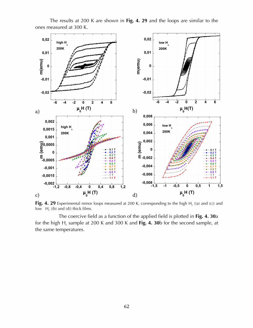
! 62!

The results at 200 K are shown in Fig. 4. 29 and the loops are similar to the

ones measured at 300 K.

a)

-0,02

-0,01

0

0,01

0,02

-6 -4 -2 0 2 4 6

m(e

mu

)

µ0H (T)

high Hc

200K

b)

-0,02

-0,01

0

0,01

0,02

-6 -4 -2 0 2 4 6

m(e

mu

)

µ0H(T)

low Hc

200K

c)

-0,002

-0,0015

-0,001

-0,0005

0

0,0005

0,001

0,0015

0,002

-1,2 -0,8 -0,4 0 0,4 0,8 1,2

0.1 T0.2 T0.3 T0.4 T0.5 T0.6 T0.7 T0.8 T0.9 T1 T1.1 T

µ0H (T)

high Hc

200K

m (

em

u)

d)

-0,008

-0,006

-0,004

-0,002

0

0,002

0,004

0,006

0,008

-1,5 -1 -0,5 0 0,5 1 1,5

0.1 T0.2 T0.3 T0.4 T0.5 T0.6 T0.7 T0.8 T0.9 T1 T1.1 T

m (

em

u)

µ0H (T)

low Hc

200K

Fig. 4. 29 Experimental minor loops measured at 200 K, corresponding to the high Hc ((a) and (c)) and low Hc ((b) and (d)) thick films.

The coercive field as a function of the applied field is plotted in Fig. 4. 30a

for the high Hc sample at 200 K and 300 K and Fig. 4. 30b for the second sample, at

the same temperatures.

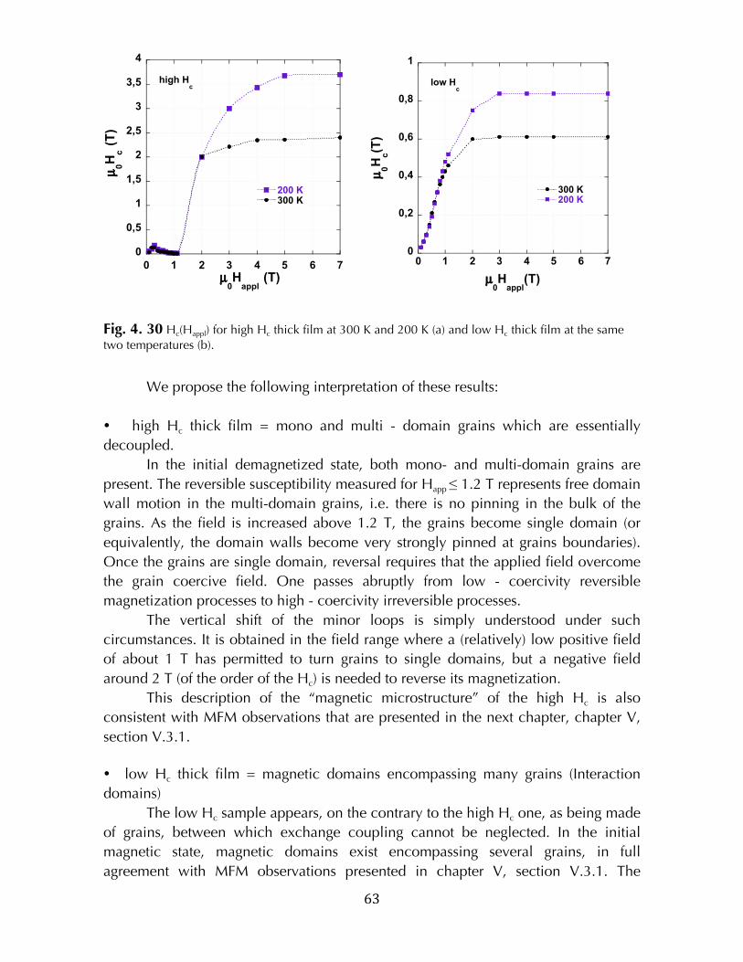
! 63!

0

0,5

1

1,5

2

2,5

3

3,5

4

0 1 2 3 4 5 6 7

200 K300 K

µ0H

c (

T)

µ0H

appl (T)

high Hc

0

0,2

0,4

0,6

0,8

1

0 1 2 3 4 5 6 7

300 K200 K

µ0H

c(T

)

µ0H

appl(T)

low Hc

Fig. 4. 30 Hc(Happl) for high Hc thick film at 300 K and 200 K (a) and low Hc thick film at the same two temperatures (b)."

We propose the following interpretation of these results:

high Hc thick film = mono and multi - domain grains which are essentially

decoupled.

In the initial demagnetized state, both mono- and multi-domain grains are

present. The reversible susceptibility measured for Happ ≤ 1.2 T represents free domain

wall motion in the multi-domain grains, i.e. there is no pinning in the bulk of the

grains. As the field is increased above 1.2 T, the grains become single domain (or

equivalently, the domain walls become very strongly pinned at grains boundaries).

Once the grains are single domain, reversal requires that the applied field overcome

the grain coercive field. One passes abruptly from low - coercivity reversible

magnetization processes to high - coercivity irreversible processes.

The vertical shift of the minor loops is simply understood under such

circumstances. It is obtained in the field range where a (relatively) low positive field

of about 1 T has permitted to turn grains to single domains, but a negative field

around 2 T (of the order of the Hc) is needed to reverse its magnetization.

This description of the “magnetic microstructure” of the high Hc is also

consistent with MFM observations that are presented in the next chapter, chapter V,

section V.3.1.

low Hc thick film = magnetic domains encompassing many grains (Interaction

domains)

The low Hc sample appears, on the contrary to the high Hc one, as being made

of grains, between which exchange coupling cannot be neglected. In the initial

magnetic state, magnetic domains exist encompassing several grains, in full

agreement with MFM observations presented in chapter V, section V.3.1. The

! 64!

microstructure seen by the domain wall is fundamentally heterogeneous and the

domain walls are expected to occupy positions where their energy is lower. A

distribution of energy barrier is expected to appear, thus explaining that irreversible

processes are found already at low applied field of approximately 2 T.

! 65!

!!!!!!!!!!!!!!!!!!!!!!!!!!!!!!!!!!!!!!!!!!!!!!!!!!!!!!!!

1 S. Heisz and G. Hilscher, JMMM 67, 20 (1987);

2 D. Givord, H. S. Li and R. Perrier de la Bâthie, Solid State Comm. 51, 857 (1984);

3 M. Sagawa, S. Fujimura, H. Yamamoto, Y. Matsuura and S. Hirosawa, J. Appl. Phys. 57, 4094 (1985);

4 K. D. Durst and H. Krönmuller, JMMM 59, 86(1986);

5 D. Givord, P. Tenaud and T. Viadieu, IEEE Trans. Magn. 24, 1921 (1988);

6 D. W. Taylor, V. Villas-Boas, Q. Lu, M.F. Rossignol, F.P. Missell, D. Givord and S. Hirosawa, JMMM 130, 225 (1994);

7 H. Krönmuller and K. D. Durst, JMMM 74, 291 (1988);

8 D. Givord, P. Tenaud and T. Viadieu, JMMM 72, 247 (1988);

9 G. Martinek and H. Krönmuller, JMMM 86, 177 (1990);

10 F. Cebollada, M. F. Rossignol and D. Givord, Phys. Rev. B 52, 13522 (1995);

11 A. N. Dobrynin, V.M.T.S Barthem and D. Givord, Appl. Phys. Lett. 95, 052511 (2009).!

!

! 66!

V. Analysis of magnetization reversal in NdFeB-based

thick films using Magnetic Force Microscopy

!

The relationship between the microstructure and the mechanism of

magnetization reversal is of great interest in permanent magnet research, as

discussed in chapter II. In this chapter, this relation is studied experimentally,

using magnetic force microscopy (MFM). It is the tool of choice for imaging

magnetic domains since it can provide good spatial resolution (50 nm

routinely)1,2,3,4 under ambient conditions. What is more, no sample preparation is

needed when imaging films if the surface is smooth enough.

The purpose of this study was to observe the evolution of the magnetic

domain structure of NdFeB-based thick films with different microstructures (and

thus different coercivities) with the applied field. The comparison of samples with

different microstructures will help us to see (indirectly) how the microstructure

influences the magnetic behavior of the materials. There have already been a

number of reports on MFM studies of NdFeB. Gouteff et al.5 and Woodcock et al.6

studied films of NdFeB in the thermally demagnetized state. Magnetization of

granular thin films deposited by PLD is reported by Neu et al.7 who identified a

nucleation type magnetization process in these films, that can be considered as an

“assembly of small micron-sized, rectangular NdFeB single crystals”8. A complete

study of magnetization and demagnetization of a die-upset NdFeB bulk magnet

with in-situ applied magnetic field was reported recently by Thielsch et al9.

Before presenting the study of domain structures of films in different states

of magnetization, the choice of the tip will be discussed and specific features

associated with MFM analysis of hard magnetic films will be reported.

V.1 Choice of the probe

The choice of the appropriate probe is an important step in MFM.

Parameters such as the coercivity of the tip’s magnetic coating and the cantilever

stiffness have to be carefully chosen as a function of the sample to be imaged.

One of the first papers reporting on the importance of the probe coating’s

coercivity is the one of Folks et al.10.

MFM imaging consists in bringing very close together two magnetic

materials – the sample on the one hand and the tip on the other hand. Naturally

there will be a magnetic interaction between them. Depending on the strength of

the interaction, three types of magnetic contrast may be considered11: charge,

susceptibility or hysteresis contrast. While the last two situations correspond to

reversible/irreversible changes in the magnetic structure of either the tip or the

sample, in the first case, no such changes are registered. We aimed for this case,

since the reduction of the number of variable parameters will ease the process of

understanding. In the second and third cases, it can be difficult to make the

difference between the information related to the sample and the information

given by the interaction between the tip and the sample since the tip and/or the

sample may change in an unpredictable way.

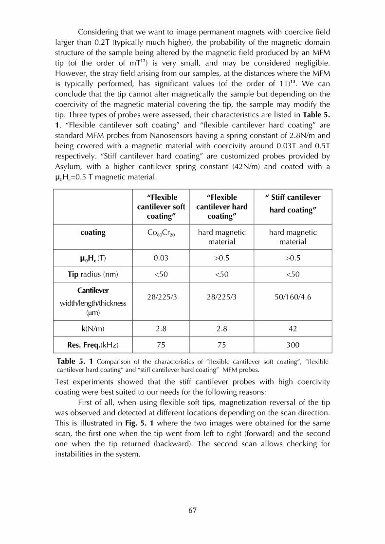
! 67!

Considering that we want to image permanent magnets with coercive field

larger than 0.2T (typically much higher), the probability of the magnetic domain

structure of the sample being altered by the magnetic field produced by an MFM

tip (of the order of mT12) is very small, and may be considered negligible.

However, the stray field arising from our samples, at the distances where the MFM

is typically performed, has significant values (of the order of 1T)13. We can

conclude that the tip cannot alter magnetically the sample but depending on the

coercivity of the magnetic material covering the tip, the sample may modify the

tip. Three types of probes were assessed, their characteristics are listed in Table 5.

1. “Flexible cantilever soft coating” and “flexible cantilever hard coating” are

standard MFM probes from Nanosensors having a spring constant of 2.8N/m and

being covered with a magnetic material with coercivity around 0.03T and 0.5T

respectively. “Stiff cantilever hard coating” are customized probes provided by

Asylum, with a higher cantilever spring constant (42N/m) and coated with a

μ0Hc=0.5 T magnetic material.

“Flexible cantilever soft

coating”

“Flexible cantilever hard

coating”

“ Stiff cantilever

hard coating”

coating Co80Cr20 hard magnetic material

hard magnetic material

μ0Hc (T) 0.03 >0.5 >0.5

Tip radius (nm) <50 <50 <50

Cantilever

width/length/thickness (µm)

28/225/3 28/225/3 50/160/4.6

k(N/m) 2.8 2.8 42

Res. Freq.(kHz) 75 75 300

Table 5. 1 Comparison of the characteristics of “flexible cantilever soft coating”, “flexible cantilever hard coating” and “stiff cantilever hard coating” MFM probes.

Test experiments showed that the stiff cantilever probes with high coercivity

coating were best suited to our needs for the following reasons:

First of all, when using flexible soft tips, magnetization reversal of the tip

was observed and detected at different locations depending on the scan direction.

This is illustrated in Fig. 5. 1 where the two images were obtained for the same

scan, the first one when the tip went from left to right (forward) and the second

one when the tip returned (backward). The second scan allows checking for

instabilities in the system.

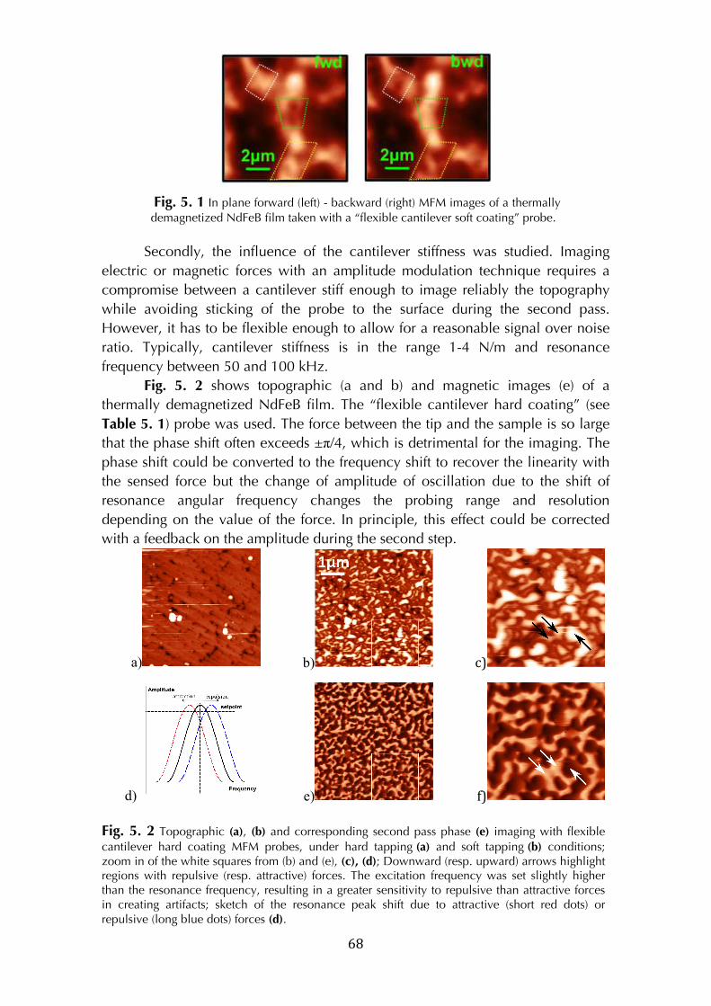
! 68!

!

Fig. 5. 1 In plane forward (left) - backward (right) MFM images of a thermally demagnetized NdFeB film taken with a “flexible cantilever soft coating” probe.

Secondly, the influence of the cantilever stiffness was studied. Imaging

electric or magnetic forces with an amplitude modulation technique requires a

compromise between a cantilever stiff enough to image reliably the topography

while avoiding sticking of the probe to the surface during the second pass.

However, it has to be flexible enough to allow for a reasonable signal over noise

ratio. Typically, cantilever stiffness is in the range 1-4 N/m and resonance

frequency between 50 and 100 kHz.

Fig. 5. 2 shows topographic (a and b) and magnetic images (e) of a

thermally demagnetized NdFeB film. The “flexible cantilever hard coating” (see

Table 5. 1) probe was used. The force between the tip and the sample is so large

that the phase shift often exceeds ±π/4, which is detrimental for the imaging. The

phase shift could be converted to the frequency shift to recover the linearity with

the sensed force but the change of amplitude of oscillation due to the shift of

resonance angular frequency changes the probing range and resolution

depending on the value of the force. In principle, this effect could be corrected

with a feedback on the amplitude during the second step.

a) ! b) ! c) !

d)! ! e) ! f) !

Fig. 5. 2 Topographic (a), (b) and corresponding second pass phase (e) imaging with flexible cantilever hard coating MFM probes, under hard tapping (a) and soft tapping (b) conditions; zoom in of the white squares from (b) and (e), (c), (d); Downward (resp. upward) arrows highlight regions with repulsive (resp. attractive) forces. The excitation frequency was set slightly higher than the resonance frequency, resulting in a greater sensitivity to repulsive than attractive forces in creating artifacts; sketch of the resonance peak shift due to attractive (short red dots) or repulsive (long blue dots) forces (d).

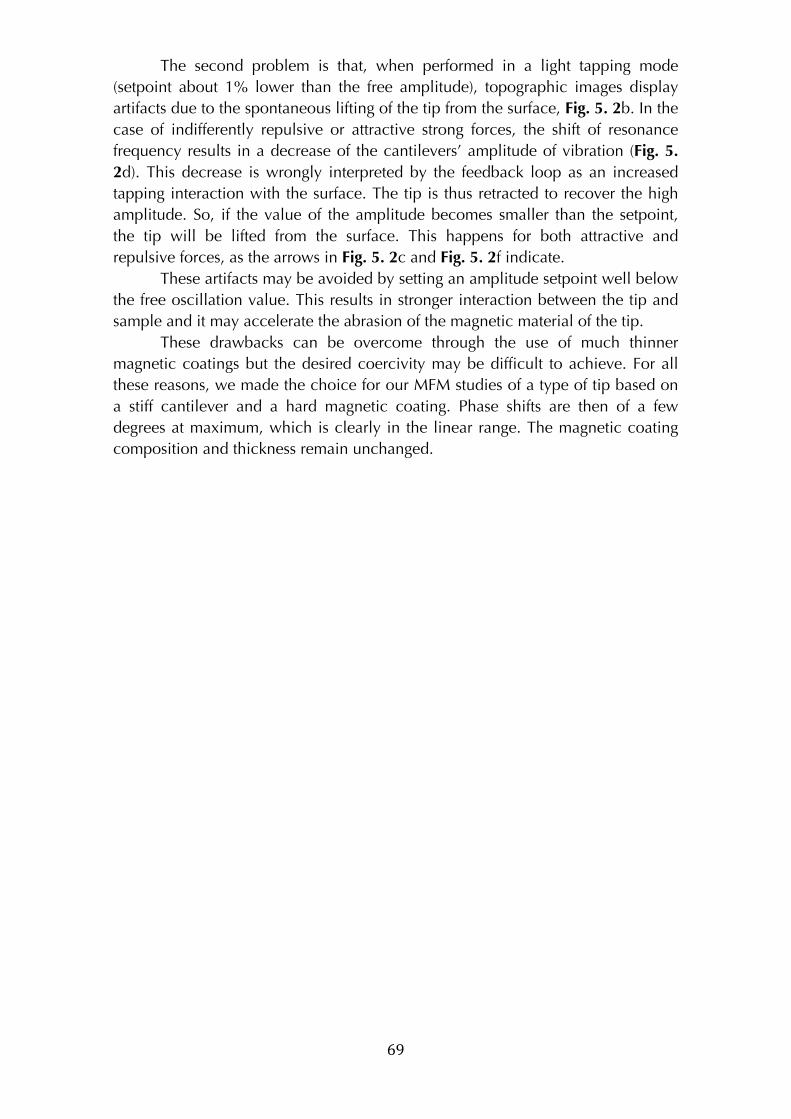
! 69!

The second problem is that, when performed in a light tapping mode

(setpoint about 1% lower than the free amplitude), topographic images display

artifacts due to the spontaneous lifting of the tip from the surface, Fig. 5. 2b. In the

case of indifferently repulsive or attractive strong forces, the shift of resonance

frequency results in a decrease of the cantilevers’ amplitude of vibration (Fig. 5.

2d). This decrease is wrongly interpreted by the feedback loop as an increased

tapping interaction with the surface. The tip is thus retracted to recover the high

amplitude. So, if the value of the amplitude becomes smaller than the setpoint,

the tip will be lifted from the surface. This happens for both attractive and

repulsive forces, as the arrows in Fig. 5. 2c and Fig. 5. 2f indicate.

These artifacts may be avoided by setting an amplitude setpoint well below

the free oscillation value. This results in stronger interaction between the tip and

sample and it may accelerate the abrasion of the magnetic material of the tip.

These drawbacks can be overcome through the use of much thinner

magnetic coatings but the desired coercivity may be difficult to achieve. For all

these reasons, we made the choice for our MFM studies of a type of tip based on

a stiff cantilever and a hard magnetic coating. Phase shifts are then of a few

degrees at maximum, which is clearly in the linear range. The magnetic coating

composition and thickness remain unchanged.

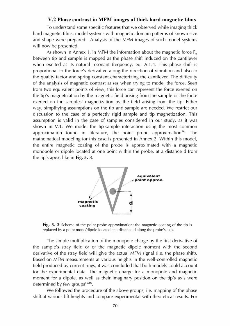
! 70!

V.2 Phase contrast in MFM images of thick hard magnetic films

To understand some specific features that we observed while imaging thick

hard magnetic films, model systems with magnetic domain patterns of known size

and shape were prepared. Analysis of the MFM images of such model systems

will now be presented.

As shown in Annex 1, in MFM the information about the magnetic force Fts

between tip and sample is mapped as the phase shift induced on the cantilever

when excited at its natural resonant frequency, eq. A.1.4. This phase shift is

proportional to the force’s derivative along the direction of vibration and also to

the quality factor and spring constant characterizing the cantilever. The difficulty

of the analysis of magnetic contrast arises when trying to model the force. Seen

from two equivalent points of view, this force can represent the force exerted on

the tip’s magnetization by the magnetic field arising from the sample or the force

exerted on the samples’ magnetization by the field arising from the tip. Either

way, simplifying assumptions on the tip and sample are needed. We restrict our

discussion to the case of a perfectly rigid sample and tip magnetization. This

assumption is valid in the case of samples considered in our study, as it was

shown in V.1. We model the tip-sample interaction using the most common

approximation found in literature, the point probe approximation14. The

mathematical modeling for this case is presented in Annex 2. Within this model,

the entire magnetic coating of the probe is approximated with a magnetic

monopole or dipole located at one point within the probe, at a distance d from

the tip’s apex, like in Fig. 5. 3.

The simple multiplication of the monopole charge by the first derivative of

the sample’s stray field or of the magnetic dipole moment with the second

derivative of the stray field will give the actual MFM signal (i.e. the phase shift).

Based on MFM measurements at various heights in the well-controlled magnetic

field produced by current rings, it was concluded that both models could account

for the experimental data. The magnetic charge for a monopole and magnetic

moment for a dipole, as well as their imaginary position on the tip’s axis were

determined by few groups15,16.

We followed the procedure of the above groups, i.e. mapping of the phase

shift at various lift heights and compare experimental with theoretical results. For

!

Fig. 5. 3 Scheme of the point probe approximation; the magnetic coating of the tip is replaced by a point mono/dipole located at a distance d along the probe’s axis.

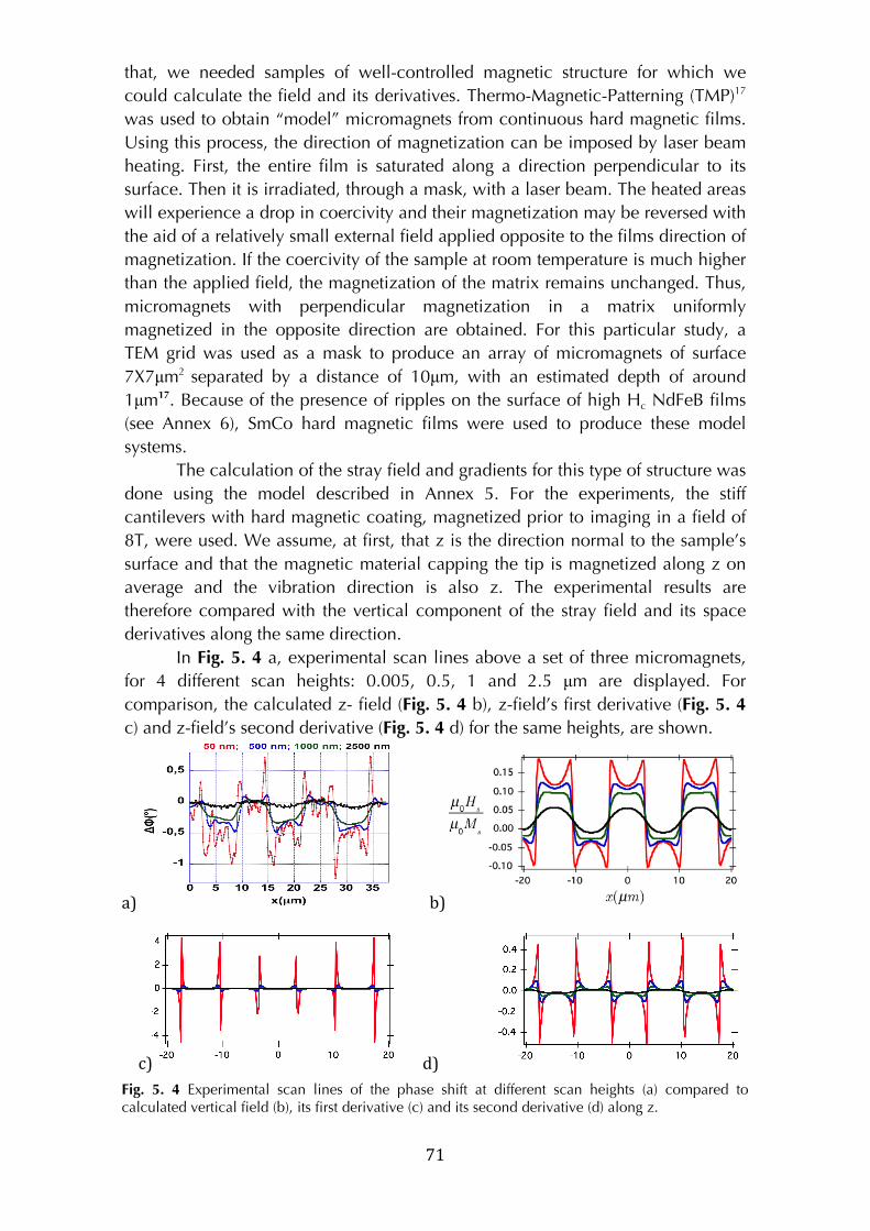
! 71!

that, we needed samples of well-controlled magnetic structure for which we

could calculate the field and its derivatives. Thermo-Magnetic-Patterning (TMP)17

was used to obtain “model” micromagnets from continuous hard magnetic films.

Using this process, the direction of magnetization can be imposed by laser beam

heating. First, the entire film is saturated along a direction perpendicular to its

surface. Then it is irradiated, through a mask, with a laser beam. The heated areas

will experience a drop in coercivity and their magnetization may be reversed with

the aid of a relatively small external field applied opposite to the films direction of

magnetization. If the coercivity of the sample at room temperature is much higher

than the applied field, the magnetization of the matrix remains unchanged. Thus,

micromagnets with perpendicular magnetization in a matrix uniformly

magnetized in the opposite direction are obtained. For this particular study, a

TEM grid was used as a mask to produce an array of micromagnets of surface

7X7µm2 separated by a distance of 10µm, with an estimated depth of around

1µm17. Because of the presence of ripples on the surface of high Hc NdFeB films

(see Annex 6), SmCo hard magnetic films were used to produce these model

systems.

The calculation of the stray field and gradients for this type of structure was

done using the model described in Annex 5. For the experiments, the stiff

cantilevers with hard magnetic coating, magnetized prior to imaging in a field of

8T, were used. We assume, at first, that z is the direction normal to the sample’s

surface and that the magnetic material capping the tip is magnetized along z on

average and the vibration direction is also z. The experimental results are

therefore compared with the vertical component of the stray field and its space

derivatives along the same direction.

In Fig. 5. 4 a, experimental scan lines above a set of three micromagnets,

for 4 different scan heights: 0.005, 0.5, 1 and 2.5 µm are displayed. For

comparison, the calculated z- field (Fig. 5. 4 b), z-field’s first derivative (Fig. 5. 4

c) and z-field’s second derivative (Fig. 5. 4 d) for the same heights, are shown.

a) ! b) !

c) ! d)!!!!!!!!!!!!! !

Fig. 5. 4 Experimental scan lines of the phase shift at different scan heights (a) compared to calculated vertical field (b), its first derivative (c) and its second derivative (d) along z.

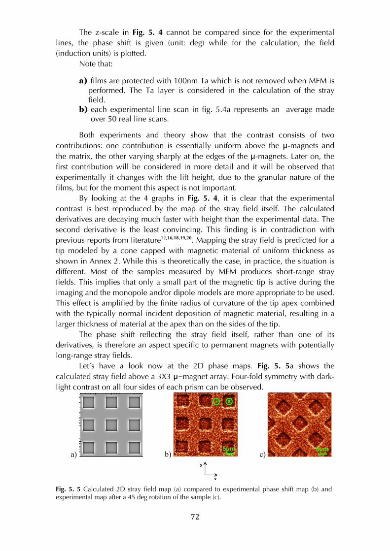
! 72!

The z-scale in Fig. 5. 4 cannot be compared since for the experimental

lines, the phase shift is given (unit: deg) while for the calculation, the field

(induction units) is plotted.

Note that:

a) films are protected with 100nm Ta which is not removed when MFM is performed. The Ta layer is considered in the calculation of the stray field.

b) each experimental line scan in fig. 5.4a represents an average made over 50 real line scans.

Both experiments and theory show that the contrast consists of two

contributions: one contribution is essentially uniform above the μ-magnets and

the matrix, the other varying sharply at the edges of the μ-magnets. Later on, the

first contribution will be considered in more detail and it will be observed that

experimentally it changes with the lift height, due to the granular nature of the

films, but for the moment this aspect is not important.

By looking at the 4 graphs in Fig. 5. 4, it is clear that the experimental

contrast is best reproduced by the map of the stray field itself. The calculated

derivatives are decaying much faster with height than the experimental data. The

second derivative is the least convincing. This finding is in contradiction with

previous reports from literature12,16,18,19,20. Mapping the stray field is predicted for a

tip modeled by a cone capped with magnetic material of uniform thickness as

shown in Annex 2. While this is theoretically the case, in practice, the situation is

different. Most of the samples measured by MFM produces short-range stray

fields. This implies that only a small part of the magnetic tip is active during the

imaging and the monopole and/or dipole models are more appropriate to be used.

This effect is amplified by the finite radius of curvature of the tip apex combined

with the typically normal incident deposition of magnetic material, resulting in a

larger thickness of material at the apex than on the sides of the tip.

The phase shift reflecting the stray field itself, rather than one of its

derivatives, is therefore an aspect specific to permanent magnets with potentially

long-range stray fields.

Let’s have a look now at the 2D phase maps. Fig. 5. 5a shows the

calculated stray field above a 3X3 μ-magnet array. Four-fold symmetry with dark-

light contrast on all four sides of each prism can be observed.

a) b) c)

Fig. 5. 5 Calculated 2D stray field map (a) compared to experimental phase shift map (b) and experimental map after a 45 deg rotation of the sample (c).

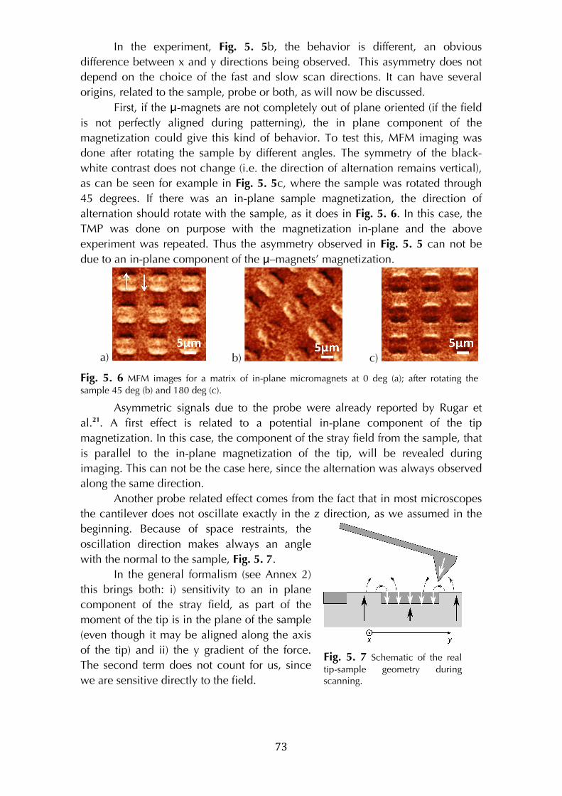
! 73!

In the experiment, Fig. 5. 5b, the behavior is different, an obvious

difference between x and y directions being observed. This asymmetry does not

depend on the choice of the fast and slow scan directions. It can have several

origins, related to the sample, probe or both, as will now be discussed.

First, if the μ-magnets are not completely out of plane oriented (if the field

is not perfectly aligned during patterning), the in plane component of the

magnetization could give this kind of behavior. To test this, MFM imaging was

done after rotating the sample by different angles. The symmetry of the black-

white contrast does not change (i.e. the direction of alternation remains vertical),

as can be seen for example in Fig. 5. 5c, where the sample was rotated through

45 degrees. If there was an in-plane sample magnetization, the direction of

alternation should rotate with the sample, as it does in Fig. 5. 6. In this case, the

TMP was done on purpose with the magnetization in-plane and the above

experiment was repeated. Thus the asymmetry observed in Fig. 5. 5 can not be

due to an in-plane component of the μ–magnets’ magnetization.

a) b) c)

Fig. 5. 6 MFM images for a matrix of in-plane micromagnets at 0 deg (a); after rotating the sample 45 deg (b) and 180 deg (c).

Asymmetric signals due to the probe were already reported by Rugar et

al.21. A first effect is related to a potential in-plane component of the tip

magnetization. In this case, the component of the stray field from the sample, that

is parallel to the in-plane magnetization of the tip, will be revealed during

imaging. This can not be the case here, since the alternation was always observed

along the same direction.

Another probe related effect comes from the fact that in most microscopes

the cantilever does not oscillate exactly in the z direction, as we assumed in the

beginning. Because of space restraints, the

oscillation direction makes always an angle

with the normal to the sample, Fig. 5. 7.

In the general formalism (see Annex 2)

this brings both: i) sensitivity to an in plane

component of the stray field, as part of the

moment of the tip is in the plane of the sample

(even though it may be aligned along the axis

of the tip) and ii) the y gradient of the force.

The second term does not count for us, since

we are sensitive directly to the field.

!

Fig. 5. 7 Schematic of the real tip-sample geometry during scanning.

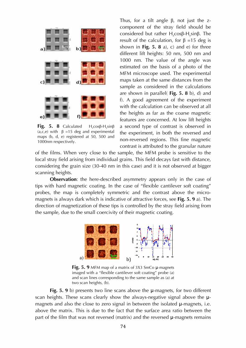
! 74!

Thus, for a tilt angle β, not just the z-

component of the stray field should be

considered but rather Hzcosβ-Hysinβ. The

result of the calculation, for β =15 deg is

shown in Fig. 5. 8 a), c) and e) for three

different lift heights: 50 nm, 500 nm and

1000 nm. The value of the angle was

estimated on the basis of a photo of the

MFM microscope used. The experimental

maps taken at the same distances from the

sample as considered in the calculations

are shown in parallel( Fig. 5. 8 b), d) and

f). A good agreement of the experiment

with the calculation can be observed at all

the heights as far as the coarse magnetic

features are concerned. At low lift heights

a second type of contrast is observed in

the experiment, in both the reversed and

non-reversed regions. This fine magnetic

contrast is attributed to the granular nature

of the films. When very close to the sample, the MFM probe is sensitive to the

local stray field arising from individual grains. This field decays fast with distance,

considering the grain size (30-40 nm in this case) and it is not observed at bigger

scanning heights.

Observation: the here-described asymmetry appears only in the case of

tips with hard magnetic coating. In the case of “flexible cantilever soft coating”

probes, the map is completely symmetric and the contrast above the micro-

magnets is always dark which is indicative of attractive forces, see Fig. 5. 9 a). The

direction of magnetization of these tips is controlled by the stray field arising from

the sample, due to the small coercivity of their magnetic coating.

a) ! b) !

Fig. 5. 9 MFM map of a matrix of 3X3 SmCo μ-magnets imaged with a “flexible cantilever soft coating” probe (a) and scan lines corresponding to the same sample as (a) at two scan heights, (b).

Fig. 5. 9 b) presents two line scans above the μ-magnets, for two different

scan heights. These scans clearly show the always-negative signal above the μ-

magnets and also the close to zero signal in between the isolated μ-magnets, i.e.

above the matrix. This is due to the fact that the surface area ratio between the

part of the film that was not reversed (matrix) and the reversed μ-magnets remains

!

!

Fig. 5. 8 Calculated Hzcosβ-Hysinβ (a,c,e) with β =15 deg and experimental maps (b, d, e) registered at 50, 500 and 1000nm respectively.

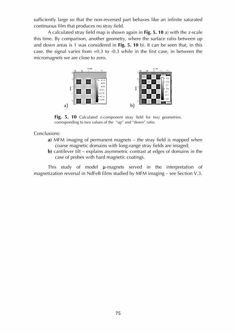
! 75!

sufficiently large so that the non-reversed part behaves like an infinite saturated

continuous film that produces no stray field.

A calculated stray field map is shown again in Fig. 5. 10 a) with the z-scale

this time. By comparison, another geometry, where the surface ratio between up

and down areas is 1 was considered in Fig. 5. 10 b). It can be seen that, in this

case, the signal varies from +0.3 to -0.3 while in the first case, in between the

micromagnets we are close to zero.

a)! ! b) !

Fig. 5. 10 Calculated z-component stray field for two geometries, corresponding to two values of the “up” and “down” ratio.

Conclusions:

a) MFM imaging of permanent magnets – the stray field is mapped when coarse magnetic domains with long-range stray fields are imaged;

b) cantilever tilt – explains asymmetric contrast at edges of domains in the case of probes with hard magnetic coatings.

This study of model μ-magnets served in the interpretation of

magnetization reversal in NdFeB films studied by MFM imaging – see Section V.3.

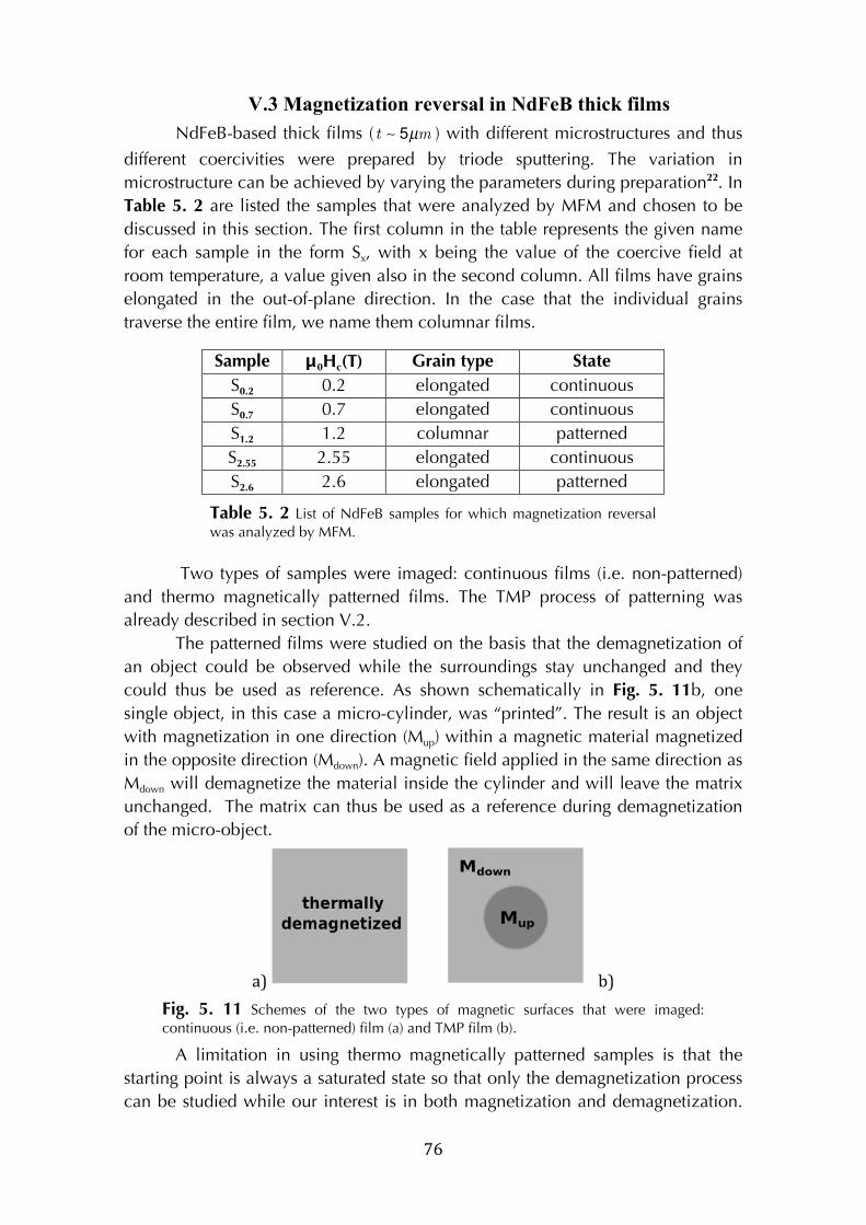
! 76!

V.3 Magnetization reversal in NdFeB thick films

NdFeB-based thick films ( t 5µm ) with different microstructures and thus

different coercivities were prepared by triode sputtering. The variation in

microstructure can be achieved by varying the parameters during preparation22. In

Table 5. 2 are listed the samples that were analyzed by MFM and chosen to be

discussed in this section. The first column in the table represents the given name

for each sample in the form Sx, with x being the value of the coercive field at

room temperature, a value given also in the second column. All films have grains

elongated in the out-of-plane direction. In the case that the individual grains

traverse the entire film, we name them columnar films.

Sample μ0Hc(T) Grain type State

S0.2 0.2 elongated continuous

S0.7 0.7 elongated continuous

S1.2 1.2 columnar patterned

S2.55 2.55 elongated continuous

S2.6 2.6 elongated patterned

Table 5. 2 List of NdFeB samples for which magnetization reversal was analyzed by MFM.

Two types of samples were imaged: continuous films (i.e. non-patterned)

and thermo magnetically patterned films. The TMP process of patterning was

already described in section V.2.

The patterned films were studied on the basis that the demagnetization of

an object could be observed while the surroundings stay unchanged and they

could thus be used as reference. As shown schematically in Fig. 5. 11b, one

single object, in this case a micro-cylinder, was “printed”. The result is an object

with magnetization in one direction (Mup) within a magnetic material magnetized

in the opposite direction (Mdown). A magnetic field applied in the same direction as

Mdown will demagnetize the material inside the cylinder and will leave the matrix

unchanged. The matrix can thus be used as a reference during demagnetization

of the micro-object.

a) b)!

Fig. 5. 11 Schemes of the two types of magnetic surfaces that were imaged: continuous (i.e. non-patterned) film (a) and TMP film (b).

A limitation in using thermo magnetically patterned samples is that the

starting point is always a saturated state so that only the demagnetization process

can be studied while our interest is in both magnetization and demagnetization.

! 77!

V.3.1 Role of the intergranular phase (S2.55 vs. S0.7)

To begin, the results obtained for two oop-textured samples, S0.7 and S2.55,

will be presented. These samples are part of the same deposit but taken from

different positions on the substrate. Due to the relatively large size of the substrate

(Si/SiO2 wafer of 10cm in diameter) and that of the target, the Nd/Fe content

varies across the wafer. Considering the results obtained from SEM, TEM, 3DAP,

VSM and XRD measurements of the two samples (see Annex 7), we tentatively

attribute the difference in coercivity to magnetic decoupling of the grains23. MFM

is used to test experimentally this assumption.

V.3.1.1 Magnetization

The first MFM images presented here, Fig. 5. 12 a) and Fig. 5. 12 b,

correspond to thermally demagnetized states of the low and high Hc samples,

respectively. The magnetic structure is similar, the width of the features observed

being in the same size range as the width of the grains. The domains in the low

coercivity sample are slightly elongated and bigger than the ones in the high

coercivity film.

A magnetic field was applied perpendicular to the sample’s surface and its

value was increased step by step. After each field application, the field was

reduced to zero and the sample was imaged in the corresponding remanent

magnetic state. The red points in Fig. 5. 13 indicate the corresponding remanent

magnetic states, for both samples (the curves were measured with the VSM).

Successive MFM images were made on the same part (10X10μm) of the

film and the results are shown in Fig. 5. 12. The bright domains in the images

correspond to those magnetic domains in the sample that are oriented in the same

direction as the applied external field and the black ones correspond to oppositely

magnetized domains.

The first steps of magnetization do not show big differences between the

samples. For applied magnetic fields smaller than 1T for S0.7 and 0.7T for S2.55, the

size of the observed features does not change significantly. This behavior is

attributed to the fact that the magnetization processes in this field range are

mainly reversible events (free magnetic domain wall movement) as could actually

be directly derived from the first magnetization curve (Fig. 5. 13). Upon

application of the magnetic field, the magnetic domain walls are moved so that

the magnetization in the field direction increases. Once the field is removed, the

walls can either move back or be pinned in some more energetically favorable

positions, depending on the value of the applied field and the microstructure of

the sample. The “remanent” state corresponding to each value of the applied field

depends on how much “freedom” to move the domain walls have. In higher

fields, the magnetic structure changes significantly: i) for the same sample with

increasing field but also ii) from one sample to the other.

In the case of S0.7, the low Hc sample, large magnetic domains

corresponding to the direction of the applied field (“white”) separated by smaller

oppositely magnetized domains (“black”) can be observed when fields superior to

2T are applied, Fig. 5. 12g, Fig. 5. 12i and Fig. 5. 12k. The white domains can

have lengths and widths of a few micrometers while the black ones are more

! 78!

elongated, with widths of maximum 2μm and lengths of a few micrometers. The

domain dimensions are significantly bigger than the width of the grains (100-150

nm from SEM images) indicating magnetic coupling between grains(i.e. the

formation of interaction domains). The area of white domains reaches a plateau

for an applied field of 2.3T. Each time the sample sees a field bigger than 2.3T,

the magnetic domains reorganize. The shape and size of the domains vary but the

ratio between up and down domains is similar. The three images just mentioned

have been binarized (Fig.5.19bis). The calculation of the ratio of white surface to

total surface gave 67.5% for 2.3 T applied field, 68 % for 4T and 74% for 8T.

The high coercivity film presents a magnetic structure that is more

granular-like for all values of the applied field (Fig. 5. 12, right column). The

smallest feature size is comparable to the grain width (200-250 nm for this

sample). The spatial extent of magnetic coupling in this sample is much reduced,

compared with the low coercivity sample. This is consistent with a better

magnetic decoupling of the grains due to the presence of a continuous non-

magnetic grain boundary phase.

Several aspects of the MFM images made following the application of the

maximum applied field, for the two samples, are considered further:

*low Hc sample ( Fig. 5. 12 k):

- the presence of big reversed domains;

- the appearance of strong black and white contrast at the

edges of the big saturated domains.

* high Hc sample (Fig. 5. 12l): granular contrast.

The presence of reversed domains in the low Hc sample after applying

even 8T can be interpreted in the following manner: the self demagnetizing field

alone is sufficient to induce nucleation at some low anisotropy defect points.

Because the grains are magnetically coupled between them (as the presence of

big magnetic domains indicate), big areas can be involved in the reversal and

they form the big black domains seen in the remanent state, even after saturation

under 8T. The reduced value of remanent magnetization, after applying 8T,

measured in the VSM is in agreement with this.

The second point related to the low Hc sample, the edge black-white

contrast is due to the tilt of the probe during MFM imaging – discussed in section

V.2.

To understand the granular contrast specific to the high Hc film, the

comparison between the two samples becomes important. Let’s consider a small

part (white square indicated in Fig. 5. 12k) of a saturated white domain in the low

coercivity sample (Fig. 5. 14a) and a similar sized part (white square in Fig. 5. 12l)

of the high coercivity one (Fig. 5. 14b). The z-scale shows that the actual

interaction between the sample and the tip – the phase shift in this case - is of the

same order of magnitude. Two line scans, corresponding to the two samples are

displayed for comparison in Fig. 5. 14c. Moreover, if the two line scans are

compared to one that corresponds to a transition from up to down domains in the

low coercivity sample (white dotted line Fig. 5. 12k), it can be seen that the

interaction is one order of magnitude higher. These three line scans are presented

together in Fig. 5. 14d.

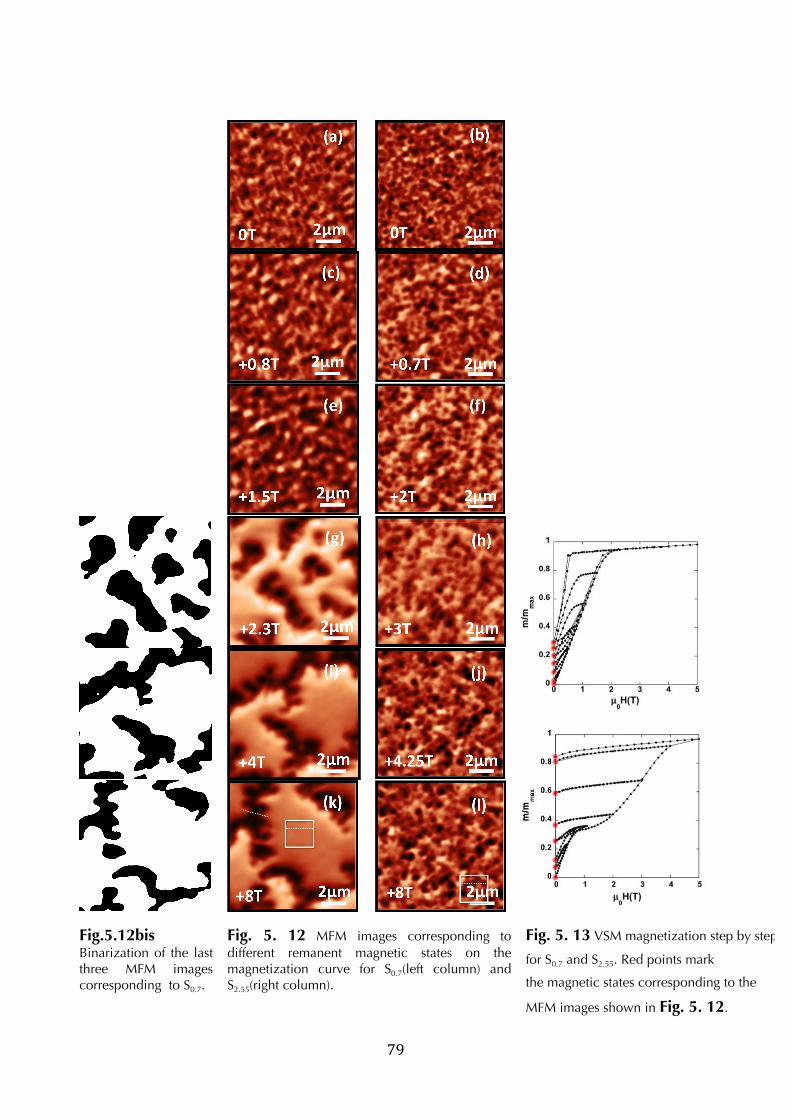
! 79!

!

! !

!

!

! !

!

!

! !

! ! !

! ! !

! ! !!

Fig.5.12bis Binarization of the last three MFM images corresponding to S0.7.

Fig. 5. 12 MFM images corresponding to different remanent magnetic states on the magnetization curve for S0.7(left column) and S2.55(right column).

!

Fig. 5. 13 VSM magnetization step by step

for S0.7 and S2.55. Red points mark

the magnetic states corresponding to the

MFM images shown in Fig. 5. 12.

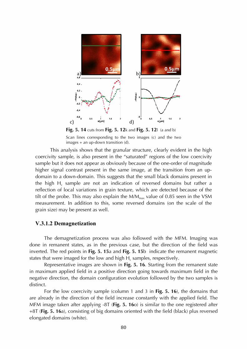
! 80!

!

a) ! b) !

c) !! d) !

Fig. 5. 14 cuts from Fig. 5. 12k and Fig. 5. 12l (a and b)

Scan lines corresponding to the two images (c) and the two images + an up-down transition (d).

This analysis shows that the granular structure, clearly evident in the high

coercivity sample, is also present in the “saturated” regions of the low coercivity

sample but it does not appear as obviously because of the one-order of magnitude

higher signal contrast present in the same image, at the transition from an up-

domain to a down-domain. This suggests that the small black domains present in

the high Hc sample are not an indication of reversed domains but rather a

reflection of local variations in grain texture, which are detected because of the

tilt of the probe. This may also explain the M/Mmax value of 0.85 seen in the VSM

measurement. In addition to this, some reversed domains (on the scale of the

grain size) may be present as well.

V.3.1.2 Demagnetization

!

The demagnetization process was also followed with the MFM. Imaging was

done in remanent states, as in the previous case, but the direction of the field was

inverted. The red points in Fig. 5. 15a and Fig. 5. 15b indicate the remanent magnetic

states that were imaged for the low and high Hc samples, respectively.

Representative images are shown in Fig. 5. 16. Starting from the remanent state

in maximum applied field in a positive direction going towards maximum field in the

negative direction, the domain configuration evolution followed by the two samples is

distinct.

For the low coercivity sample (column 1 and 3 in Fig. 5. 16), the domains that

are already in the direction of the field increase constantly with the applied field. The

MFM image taken after applying -8T (Fig. 5. 16o) is similar to the one registered after

+8T (Fig. 5. 16a), consisting of big domains oriented with the field (black) plus reversed

elongated domains (white).

! 81!

For the high Hc sample (column 2 and 4 in Fig. 5. 16), the reversal proceeds in a

different manner. In the beginning, small reversed nuclei (a few grains wide) form in

different parts of the sample. When the field is increased two things happen: i)

formation of new reversed zones and ii) a slight increase in the size of the already

existing nuclei. This is evidence for the already-mentioned magnetic decoupling of the

grains in these samples.

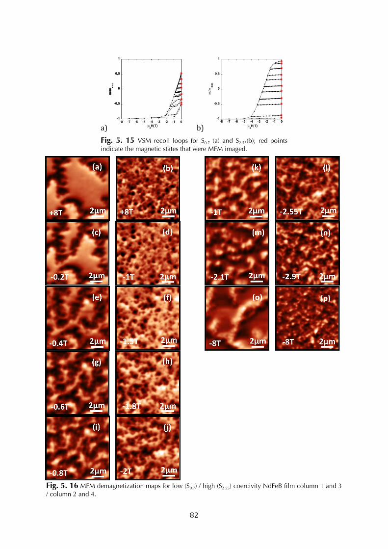
! 82!

a) ! b) !

Fig. 5. 15 VSM recoil loops for S0.7 (a) and S2.55(b); red points indicate the magnetic states that were MFM imaged.

! !

! !

! !

! !

! !

! !

! !

! !

Fig. 5. 16 MFM demagnetization maps for low (S0.7) / high (S2.55) coercivity NdFeB film column 1 and 3 / column 2 and 4.

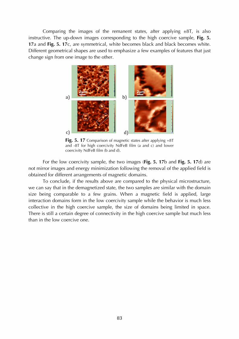
! 83!

Comparing the images of the remanent states, after applying ±8T, is also

instructive. The up-down images corresponding to the high coercive sample, Fig. 5.

17a and Fig. 5. 17c, are symmetrical, white becomes black and black becomes white.

Different geometrical shapes are used to emphasize a few examples of features that just

change sign from one image to the other.

a)! ! b)! !

c)! ! d) !

Fig. 5. 17 Comparison of magnetic states after applying +8T and -8T for high coercivity NdFeB film (a and c) and lower coercivity NdFeB film (b and d).

For the low coercivity sample, the two images (Fig. 5. 17b and Fig. 5. 17d) are

not mirror images and energy minimization following the removal of the applied field is

obtained for different arrangements of magnetic domains.

To conclude, if the results above are compared to the physical microstructure,

we can say that in the demagnetized state, the two samples are similar with the domain

size being comparable to a few grains. When a magnetic field is applied, large

interaction domains form in the low coercivity sample while the behavior is much less

collective in the high coercive sample, the size of domains being limited in space.

There is still a certain degree of connectivity in the high coercive sample but much less

than in the low coercive one.

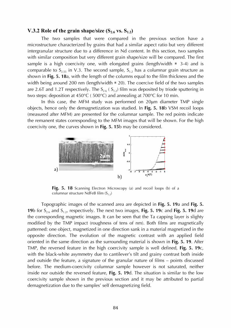
! 84!

V.3.2 Role of the grain shape/size (S2.6 vs. S1.2)

The two samples that were compared in the previous section have a

microstructure characterized by grains that had a similar aspect ratio but very different

intergranular structure due to a difference in Nd content. In this section, two samples

with similar composition but very different grain shape/size will be compared. The first

sample is a high coercivity one, with elongated grains (length/width 3-4) and is

comparable to S2.55 in V.3. The second sample, S1.2 has a columnar grain structure as

shown in Fig. 5. 18a, with the length of the columns equal to the film thickness and the

width being around 200 nm (length/width 20). The coercive field of the two samples

are 2.6T and 1.2T respectively. The S2.6 ( S1.2) film was deposited by triode sputtering in

two steps: deposition at 450°C ( 500°C) and annealing at 700°C for 10 min.

In this case, the MFM study was performed on 20µm diameter TMP single

objects, hence only the demagnetization was studied. In Fig. 5. 18b VSM recoil loops

(measured after MFM) are presented for the columnar sample. The red points indicate

the remanent states corresponding to the MFM images that will be shown. For the high

coercivity one, the curves shown in Fig. 5. 15b may be considered.

a)! !

b) !

Fig. 5. 18 Scanning Electron Microscopy (a) and recoil loops (b) of a columnar structure NdFeB film (S1.2)

Topographic images of the scanned area are depicted in Fig. 5. 19a and Fig. 5.

19b for S2.6 and S1.2, respectively. The next two images, Fig. 5. 19c and Fig. 5. 19d are

the corresponding magnetic images. It can be seen that the Ta capping layer is slighty

modified by the TMP impact (roughness of tens of nm). Both films are magnetically

patterned: one object, magnetized in one direction sank in a material magnetized in the

opposite direction. The evolution of the magnetic contrast with an applied field

oriented in the same direction as the surrounding material is shown in Fig. 5. 19. After

TMP, the reversed feature in the high coercivity sample is well defined, Fig. 5. 19c,

with the black-white asymmetry due to cantilever’s tilt and grainy contrast both inside

and outside the feature, a signature of the granular nature of films – points discussed

before. The medium-coercivity columnar sample however is not saturated, neither

inside nor outside the reversed feature, Fig. 5. 19d. The situation is similar to the low

coercivity sample shown in the previous section and it may be attributed to partial

demagnetization due to the samples’ self demagnetizing field.

!

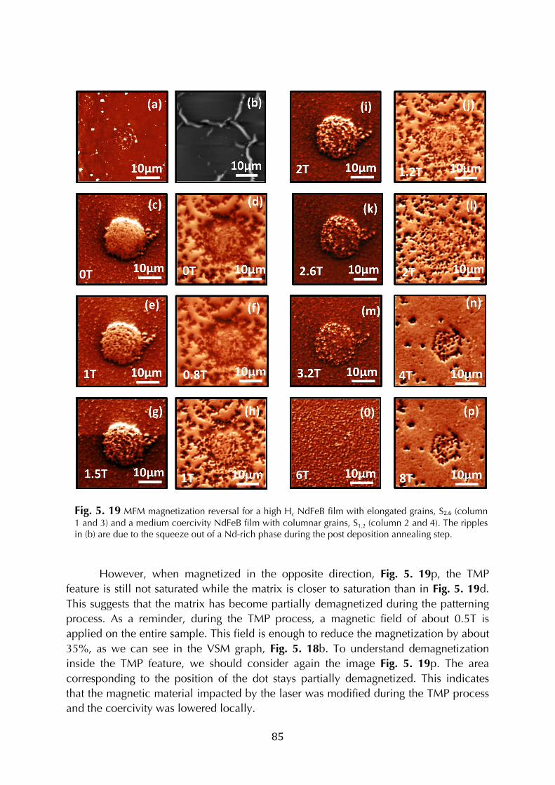
! 85!

!

However, when magnetized in the opposite direction, Fig. 5. 19p, the TMP

feature is still not saturated while the matrix is closer to saturation than in Fig. 5. 19d.

This suggests that the matrix has become partially demagnetized during the patterning

process. As a reminder, during the TMP process, a magnetic field of about 0.5T is

applied on the entire sample. This field is enough to reduce the magnetization by about

35%, as we can see in the VSM graph, Fig. 5. 18b. To understand demagnetization

inside the TMP feature, we should consider again the image Fig. 5. 19p. The area

corresponding to the position of the dot stays partially demagnetized. This indicates

that the magnetic material impacted by the laser was modified during the TMP process

and the coercivity was lowered locally.

! !

! !

! !

! !

! !

! ! !

! !

! !

Fig. 5. 19 MFM magnetization reversal for a high Hc NdFeB film with elongated grains, S2.6 (column 1 and 3) and a medium coercivity NdFeB film with columnar grains, S1.2 (column 2 and 4). The ripples in (b) are due to the squeeze out of a Nd-rich phase during the post deposition annealing step.

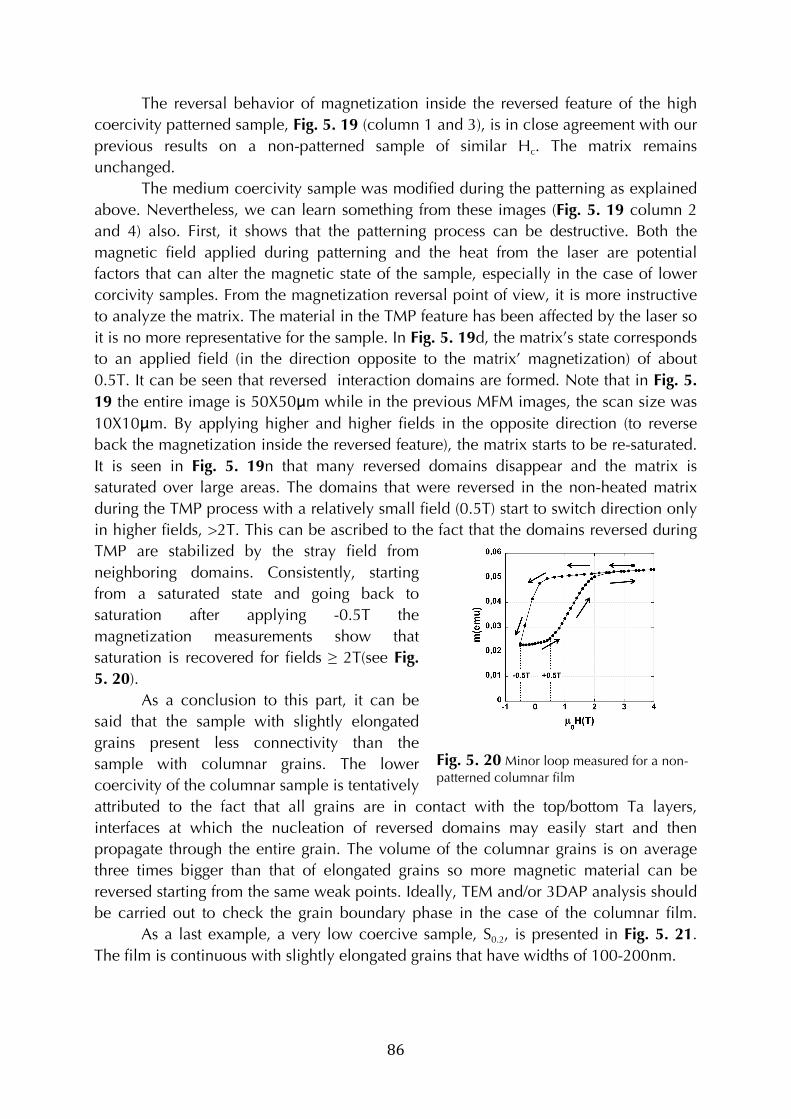
! 86!

The reversal behavior of magnetization inside the reversed feature of the high

coercivity patterned sample, Fig. 5. 19 (column 1 and 3), is in close agreement with our

previous results on a non-patterned sample of similar Hc. The matrix remains

unchanged.

The medium coercivity sample was modified during the patterning as explained

above. Nevertheless, we can learn something from these images (Fig. 5. 19 column 2

and 4) also. First, it shows that the patterning process can be destructive. Both the

magnetic field applied during patterning and the heat from the laser are potential

factors that can alter the magnetic state of the sample, especially in the case of lower

corcivity samples. From the magnetization reversal point of view, it is more instructive

to analyze the matrix. The material in the TMP feature has been affected by the laser so

it is no more representative for the sample. In Fig. 5. 19d, the matrix’s state corresponds

to an applied field (in the direction opposite to the matrix’ magnetization) of about

0.5T. It can be seen that reversed interaction domains are formed. Note that in Fig. 5.

19 the entire image is 50X50μm while in the previous MFM images, the scan size was

10X10μm. By applying higher and higher fields in the opposite direction (to reverse

back the magnetization inside the reversed feature), the matrix starts to be re-saturated.

It is seen in Fig. 5. 19n that many reversed domains disappear and the matrix is

saturated over large areas. The domains that were reversed in the non-heated matrix

during the TMP process with a relatively small field (0.5T) start to switch direction only

in higher fields, >2T. This can be ascribed to the fact that the domains reversed during

TMP are stabilized by the stray field from

neighboring domains. Consistently, starting

from a saturated state and going back to

saturation after applying -0.5T the

magnetization measurements show that

saturation is recovered for fields ≥ 2T(see Fig.

5. 20).

As a conclusion to this part, it can be

said that the sample with slightly elongated

grains present less connectivity than the

sample with columnar grains. The lower

coercivity of the columnar sample is tentatively

attributed to the fact that all grains are in contact with the top/bottom Ta layers,

interfaces at which the nucleation of reversed domains may easily start and then

propagate through the entire grain. The volume of the columnar grains is on average

three times bigger than that of elongated grains so more magnetic material can be

reversed starting from the same weak points. Ideally, TEM and/or 3DAP analysis should

be carried out to check the grain boundary phase in the case of the columnar film.

As a last example, a very low coercive sample, S0.2, is presented in Fig. 5. 21.

The film is continuous with slightly elongated grains that have widths of 100-200nm.

Fig. 5. 20 Minor loop measured for a non-patterned columnar film

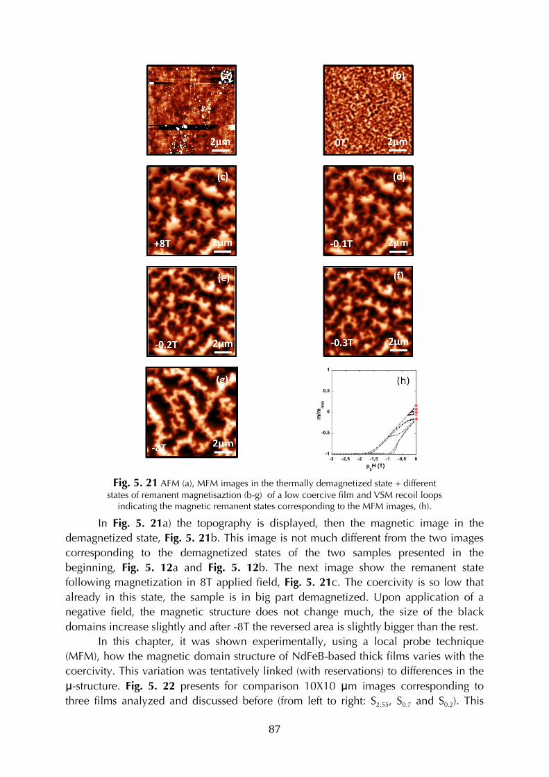
! 87!

! !

! !

! !

!

!

Fig. 5. 21 AFM (a), MFM images in the thermally demagnetized state + different states of remanent magnetisaztion (b-g) of a low coercive film and VSM recoil loops

indicating the magnetic remanent states corresponding to the MFM images, (h).

In Fig. 5. 21a) the topography is displayed, then the magnetic image in the

demagnetized state, Fig. 5. 21b. This image is not much different from the two images

corresponding to the demagnetized states of the two samples presented in the

beginning, Fig. 5. 12a and Fig. 5. 12b. The next image show the remanent state

following magnetization in 8T applied field, Fig. 5. 21c. The coercivity is so low that

already in this state, the sample is in big part demagnetized. Upon application of a

negative field, the magnetic structure does not change much, the size of the black

domains increase slightly and after -8T the reversed area is slightly bigger than the rest.

In this chapter, it was shown experimentally, using a local probe technique

(MFM), how the magnetic domain structure of NdFeB-based thick films varies with the

coercivity. This variation was tentatively linked (with reservations) to differences in the

μ-structure. Fig. 5. 22 presents for comparison 10X10 μm images corresponding to

three films analyzed and discussed before (from left to right: S2.55, S0.7 and S0.2). This

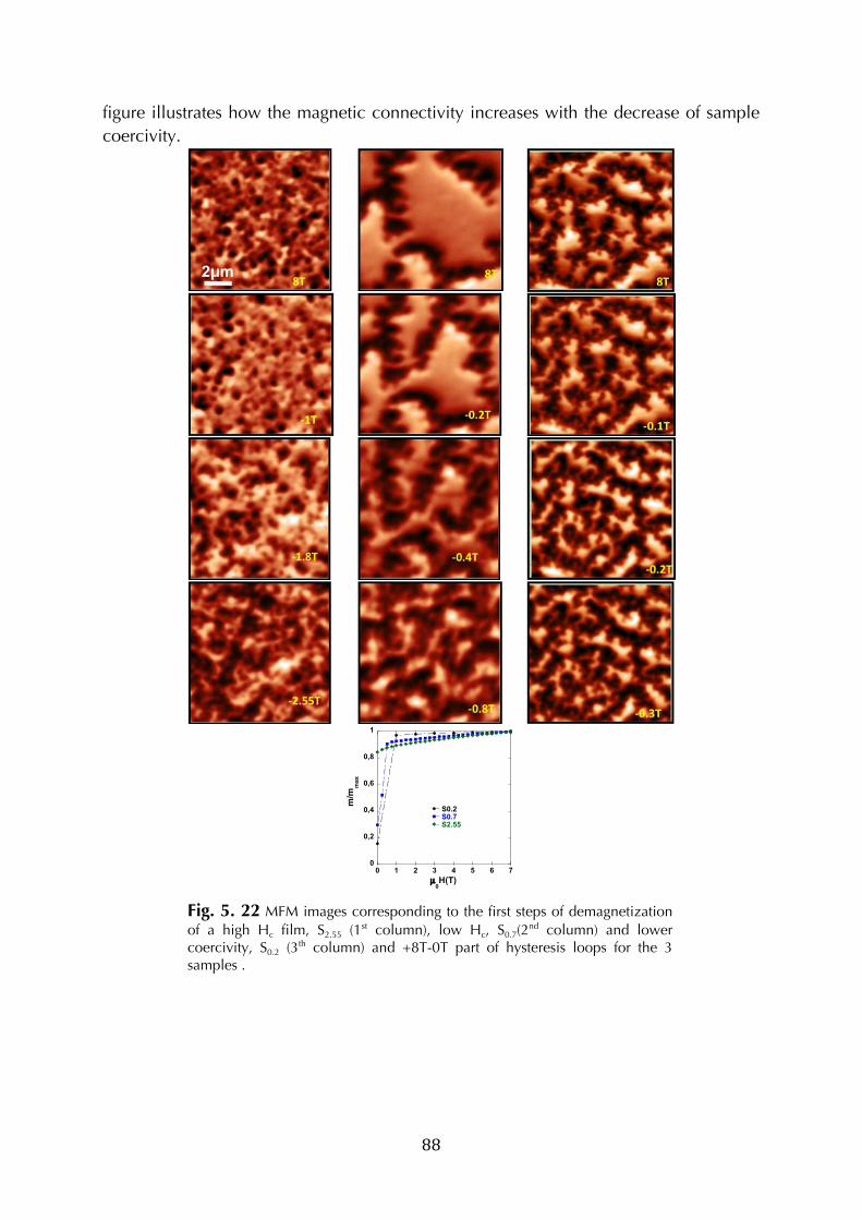
! 88!

figure illustrates how the magnetic connectivity increases with the decrease of sample

coercivity.

! ! !

! ! !

! ! !

! ! !

0

0,2

0,4

0,6

0,8

1

0 1 2 3 4 5 6 7

S0.2S0.7S2.55

m/m

max

µ0H(T)

!

Fig. 5. 22 MFM images corresponding to the first steps of demagnetization of a high Hc film, S2.55 (1st column), low Hc, S0.7(2

nd column) and lower coercivity, S0.2 (3th column) and +8T-0T part of hysteresis loops for the 3 samples .

! 89!

!!!!!!!!!!!!!!!!!!!!!!!!!!!!!!!!!!!!!!!!!!!!!!!!!!!!!!!!

1 Y. Martin, D. Rugar and H. K. Wickramasinghe, Appl. Phys. Lett. 52, 244 (1988);

2 H.J. Mamin, D. Rugar, J. E. Stern, R. E. Fontana and P. Kasiraj, Appl. Phys. Lett. 55, 318 (1989);

3 A. DiCarlo, M. R. Scheinfein and R. V. Chamberlin, Appl. Phys. Lett. 61, 2108 (1992);

4 L. Abelmann, S. Porthun, M. Haast, C. Lodder, A. Moser, M. E. Best, P. J.A van Schendel, B. Stiefel, H. J. Hug, G. P. Heydon, A. Farley, S. R. Hoon, T. Pfaffelhuber, R. Proksch and K. Babcock, JMMM 190, 135 (1998);

5 P.C. Gouteff, l. Folks and R. Street, JMMM 177-181, 1241-1242 (1998);

6 T.G. Woodcock, K. Khopkov, A. Walther, N. M. Dempsey, D. Givord, L. Schultz and O. Gutfleisch, Scripta Mat. 60, 826 (2009);

7 V. Neu, F. Grosmann, S. Melcher, S. Fähler and L. Schultz, JMMM 290-291, 1263-1266 (2005);

8 V. Neu, S. Melcher, U. Hannemann, S. Fähler and L. Schultz, Phys.Rev.B 70, 144418 (2004);

9 J. Thielsch, H. Stopfel, U. Wolff, V. Neu, T. G. Woodcock, K. Güth, L. Schultz and O. Gutfleisch, J. Appl. Phys. 111, 103901 (2012);

10 L. Folks and R. C. Woodward, JMMM 190, 28 (1998);

11 A. Hubert, W. Rave and S. L. Tomlinson, Phys. Stat. Sol. (b) 204, 817 (1997);

12 R. Engel-Herbert, D. M. Schaadt and T. Hesjedal, J. Appl. Phys. 99, 113905 (2006);

13 M. Kustov, P. Laczkowski, D. Hykel, K. Hasselbach, F. Dumas-Bouchiat, D. O’Brien, P. Kauffmann, R. Grechishkin, D. Givord, G. Reyne, O. Cugat and N. M. Dempsey, J. Appl. Phys. 108, 063914 (2010);

14 U. Hartmann, Phys. Lett. A 137, 475 (1989);

15 L. Kong and S. Y. Chou, Appl. Phys. Lett. 70, 2043 (1997);

16 J. Lohau, S. Kirsch, A. Carl, G. Dumpich and E. F. Wassermann, J. Appl. Phys. 86, 3410 (1999);

17 F. Dumas-Bouchiat, L. F. Zanini, M. Kustov, N. M. Dempsey, R. Grechishkin, K. Hasselbach, J. C. Orlianges, C. Champeaux, A. Catherinot and D. Givord, Appl. Phys. Lett. 96, 102511 (2010);

18 A. Wadas and H. J. Güntherodt, Phys. Lett. A 146, 277 (1990);

19 T. Arie, N. Yoshida, S. Akita and Y. Nakayama, J. Phys. D: Appl. Phys. 34, L43 (2001);

! 90!

!!!!!!!!!!!!!!!!!!!!!!!!!!!!!!!!!!!!!!!!!!!!!!!!!!!!!!!!

20 T. E. Schäffer, M. Radmacher and R. Proksch, J. Appl. Phys. 94, 6525 (2003);

21 D. Rugar, H. J. Mamin, G. Guethner, S. E. Lambert, J. E. Stern, I. McFadyen and T. Yogi, J. Appl. Phys. 68, 1169 (1990);

22 N. M. Dempsey, A. Walther, F. May and D. Givord, Appl. Phys. Lett. 90, 092509 (2007).!

23 N. M. Dempsey, T. G. Woodcock, H. Sepehri-Amin, Y. Zhang, H. Kennedy, D. Givord, K. Hono and O. Gutfleisch, Acta Materialia, accepted (2013);

!

! 91!

VI. Conclusions and perspectives

Conclusions

This thesis work concerned the study of magnetization reversal in NdFeB -

based magnets, with the aim to better understand and thus improve coercivity in

these technologically important materials. Magnetization reversal was studied

using both “global” (magnetometry) and “local probe” (magnetic force

microscopy) techniques. Two types of samples were considered: bulk magnets

provided by the Toyota Motor Corporation, and thick film magnets prepared at

Institut Néel, within the framework of this thesis. An original infiltration process

had been applied to the bulk magnets to introduce a NdCu grain boundary phase,

which resulted in an increase in coercivity. The main results of this work will now

be recalled:

Thick films as model systems

Thick films may be considered as model systems in which the μ-structure

can be modified by varying different process parameters (film composition,

deposition temperature…). During this work, triode sputtering was used to

prepare highly textured NdFeB films (typical thickness around 5 µm) with

coercivity ranging in value from 2.7 T down to 0.2 T. The grain shape was varied

from equiaxed to columnar.

- Coercivity analysis

The first major part of the work concerned the development of coercivity

analysis in both the bulk and thick film samples. The aim here was to assess

whether phenomenological models (the Micro-Magnetic Model “MM” and the

Global Model “GM”) could be used to characterize the behavior of these hard

magnetic materials. Two distinct contributions are considered in coercivity

analysis: i) the “α” parameter that concerns the region where the reversed nucleus

is formed, ii) a demagnetizing field parameter (“N”) that is associated with the

heterogeneous nature of the hard magnetic material.

Analysis of the bulk samples within both the Micro-Magnetic Model and

the Global Model shows that the change in coercivity owing to the infiltration

process is associated with a change in the demagnetizing field parameter (N),

while the parameter characterizing the formation of a reversed domain is

essentially unchanged. This suggests that coercivity enhancement is not due to a

modification of the nucleation process, but may be associated with decoupling of

the main phase grains, in agreement with microstructural observations. Strikingly,

at a given temperature, the activation volume is very similar for the different

samples.

In the films, on the contrary, the activation volume is found to differ, the

higher the coercivity, the lower the activation volume. Note that this behavior is

in agreement with the so-called “Barbier plot”, according to which the inverse of

the activation volume varies as the coercivity.

! 92!

Analysis of the angular dependence of coercivity is in agreement with

previous studies of bulk NdFeB magnets, showing that coercivity is not governed

by coherent rotation but expansion of a preformed nucleus. This is compatible

with the notion of “pinning”, but also with that of “passage-expansion”.

In all cases, the fact that the global model gives a fair account of the

temperature dependence of coercivity and activation volume, implies that the

magnetic properties within the activation volume are close to those of the main

phase. This hypothesis, which has been debated for a long time, has recently

received support from numerical modeling.

- Magnetic Force Microscopy

The second major part of this thesis concerned a study of magnetization

processes in thick films of NdFeB, using magnetic force microscopy. As part of

this study, we examined specific aspects of the MFM imaging of hard magnet

films. We demonstrated that mechanically stiff MFM probes coated with a hard

magnetic material are best suited to the study of thick hard magnetic films, owing

to strong probe-sample interactions. One consequence of using hard magnetic

probes is the detection of an in-plane component of the sample’s stray field, due

to the inclination of the probe during scanning. By comparing experimental

results with calculated field profiles of model micro-magnets prepared using a

thermomagnetic patterning technique, it was found that in the case of permanent

magnet films with coarse magnetic domains (and thus long-range stray fields) the

stray field of the sample, as opposed to it’s derivatives, is imaged in MFM.

Magnetization and demagnetization of NdFeB-based films with different

values of coercivity and different microstructures was studied using the MFM. The

magnetic domain structure of the thermally demagnetized state is similar for all

the samples, irrespective of their coercivity. On the contrary, the

magnetization/demagnetization behavior is seen to depend on the coercivity. In

low fields, reversible events occur, so that the remanent domain structures do not

evolve much, in agreement with the minor hysteresis loop analysis carried out on

high and low coercivity films in the magnetometer. However, after application of

higher fields, the remanent domain structures are coercivity dependent. Large

interaction domains are clearly observed to develop in the low coercivity sample,

while high coercivity samples are characterized by a fine granular magnetic

structure. Note that the persistence of this granular structure, even after the

application of 8 T, when the film is practically saturated, may be explained by the

sensitivity of the hard MFM tip to in-plane field components associated with local

variations in the alignment of individual grains. The collective nature of reversal

seen in the magnetization and demagnetization sweeps of medium to low

coercivity samples is due to exchange coupling between grains. This results from

direct contact between neighboring hard magnetic grains. Magnetization reversal

in the high coercivity films, which are known to have continuous Nd-rich grain

boundary phases, occurs by a mixture of nucleation and growth of existing

reversed domains.

! 93!

Perspectives

Based on recent progress made by a number of groups with grain boundary

engineering of NdFeB magnets, there is much potential to further increase the

coercivity of this technologically important material. Films may be considered as

model samples, in which the microstructure can be controlled through various

processing parameters. Multi-phase structures may be produced by the annealing

of single layer alloy deposits or alternatively multi-layer deposition may be used

to directly produce a multi-phase architecture in which the composition and

thickness of the individual phases is controlled. Multi-layer deposition also allows

for the study of diffusion between phases or along grain boundaries.

As an example of multi-phase structures produced by the annealing of

single layer alloy deposits, some preliminary experiments have been carried out in

the framework of this thesis, to study the influence of the addition of Cu in Nd-

rich NdFeB films (in this case, a piece of Cu was added to the NdFeB target).

Results presented in Annex 9, confirm the positive benefit of adding Cu on the

coercivity of NdFeB thick films. Further structural (TEM, 3DAP) and magnetic

(coercivity analysis, MFM..) studies are required to better understand and optimize

this approach. Controlled diffusion in multi-layer structures has also begun. We

think that these various film-based approaches hold much potential for the

development of magnets with reduced RE-content, including RE-lean hard-soft

nanocomposites, as well as RE-free materials.

Concerning coercivity analysis, this could be further developed together

with micro-magnetic simulations that take into account thermal activation effects.

We believe that the activation volume is an important parameter to be considered

in the study of magnetization reversal in hard magnetic materials.

Magnetic Force Microscopy is a powerful tool that may serve in the

understanding of magnetization reversal. In the case of thick films, imaging of the

cross section of films should shed more light on the influence of grain shape and

interfaces on reversal. The development of quantitative MFM imaging, with the

use of probes of known magnetization, is also of interest.

The development of permanent magnets relies on a triangular approach

combining sample preparation, characterization (structural and magnetic) and

modeling. Recent advances in all three domains (press-less processing,

infiltration, thin and thick film processing; atomic scale resolution imaging (TEM,

3DAP), MFM imaging under high field; molecular dynamics and micromagnetic

simulations including thermal activation) has already led to significant

improvements in the extrinsic properties achievable, and holds the key to

improving our understanding of these materials.

!

! 94!

Annex 1. Model of an AFM cantilever

We recall the usual description of a cantilever for atomic force microscopy

with a harmonic oscillator along a direction with coordinate z, with inertia m,

stiffness k and damping Γ, subject to an external force F:

(A1. 1)!

This description is very adequate for the physics of magnetic force

microscopy. F may contain the cantilever excitation at a given angular frequency

ω, as well as the force created by the sample Fts. The latter is classically expanded

to first order to remain within the frame of a harmonic oscillator. As dF/dz is

much smaller than the cantilever stiffness, this results simply in a linear shift of the

resonance angular frequency from its natural value, , to

. In magnetic force microscopy the information about the

magnetic force is then mapped as the phase shift induced on the cantilever when

excited at :

(A1. 2)

is the quality factor of the cantilever.

The linear relationship in (A1. 2 remains valid as long as the phase shift is

reasonably smaller than π/4. As the force is the gradient of energy, we may rewrite

the phase shift as:

(A1. 3)

This expression is particularly useful for the analysis of magnetic forces.

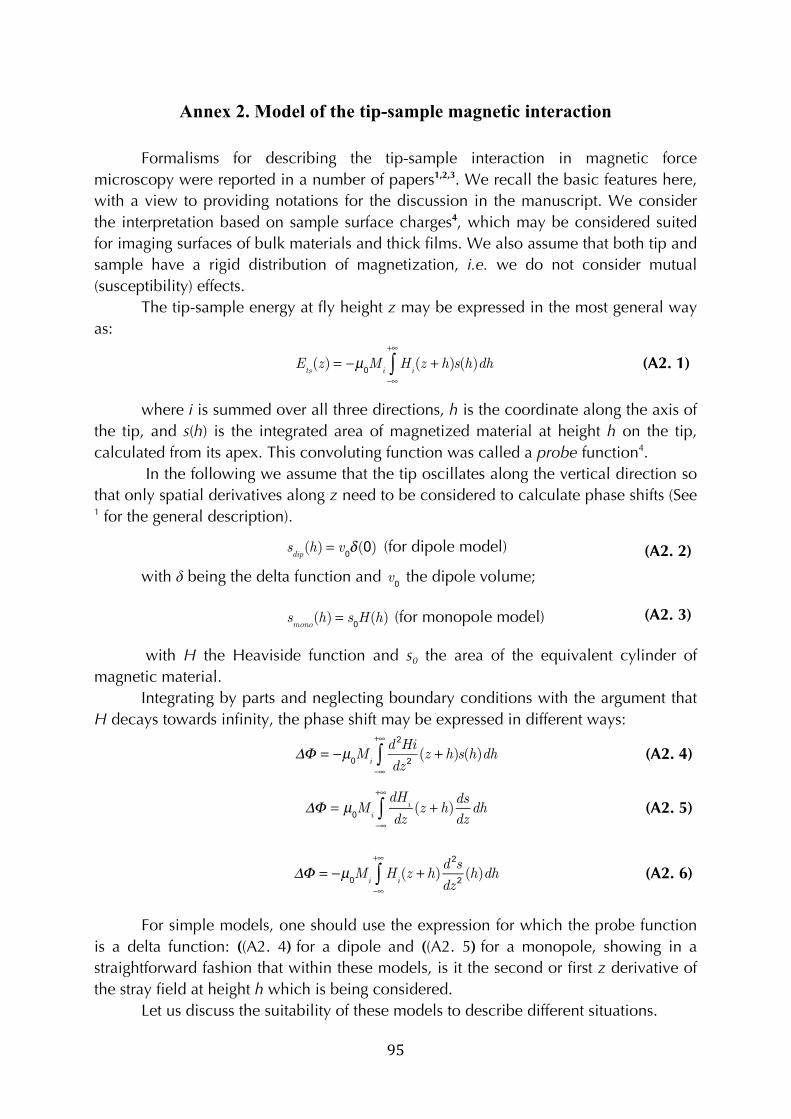
! 95!

Annex 2. Model of the tip-sample magnetic interaction

Formalisms for describing the tip-sample interaction in magnetic force

microscopy were reported in a number of papers1,2,3. We recall the basic features here,

with a view to providing notations for the discussion in the manuscript. We consider

the interpretation based on sample surface charges4, which may be considered suited

for imaging surfaces of bulk materials and thick films. We also assume that both tip and

sample have a rigid distribution of magnetization, i.e. we do not consider mutual

(susceptibility) effects.

The tip-sample energy at fly height z may be expressed in the most general way

as:

Ets(z) = −µ

0M

iH

i(z + h)s(h)dh

−∞

+∞

∫ (A2. 1)

where i is summed over all three directions, h is the coordinate along the axis of

the tip, and s(h) is the integrated area of magnetized material at height h on the tip,

calculated from its apex. This convoluting function was called a probe function4.

In the following we assume that the tip oscillates along the vertical direction so

that only spatial derivatives along z need to be considered to calculate phase shifts (See 1 for the general description).

s

dip(h) = v

0δ(0) (for dipole model) (A2. 2)

with δ being the delta function and v

0 the dipole volume;

s

mono(h) = s

0H(h) (for monopole model) (A2. 3)

with H the Heaviside function and s0 the area of the equivalent cylinder of

magnetic material.

Integrating by parts and neglecting boundary conditions with the argument that

H decays towards infinity, the phase shift may be expressed in different ways:

ΔΦ = −µ0M

i

d2Hi

dz2

(z + h)s(h)dh

−∞

+∞

∫ (A2. 4)

ΔΦ = µ0M

i

dHi

dz(z + h)

ds

dzdh

−∞

+∞

∫ (A2. 5)

ΔΦ = −µ0M

iH

i(z + h)

d2s

dz2(h)dh

−∞

+∞

∫ (A2. 6)

For simple models, one should use the expression for which the probe function

is a delta function: ((A2. 4) for a dipole and ((A2. 5) for a monopole, showing in a

straightforward fashion that within these models, is it the second or first z derivative of

the stray field at height h which is being considered.

Let us discuss the suitability of these models to describe different situations.

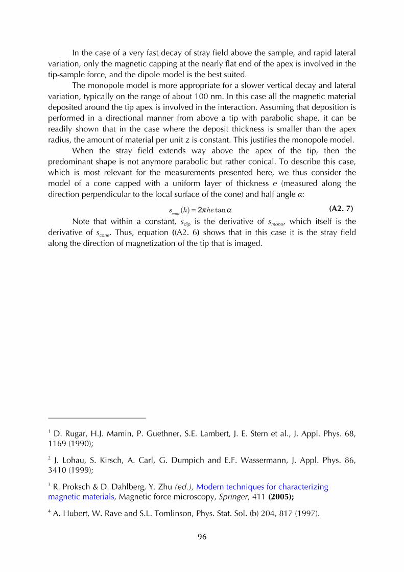
! 96!

In the case of a very fast decay of stray field above the sample, and rapid lateral

variation, only the magnetic capping at the nearly flat end of the apex is involved in the

tip-sample force, and the dipole model is the best suited.

The monopole model is more appropriate for a slower vertical decay and lateral

variation, typically on the range of about 100 nm. In this case all the magnetic material

deposited around the tip apex is involved in the interaction. Assuming that deposition is

performed in a directional manner from above a tip with parabolic shape, it can be

readily shown that in the case where the deposit thickness is smaller than the apex

radius, the amount of material per unit z is constant. This justifies the monopole model.

When the stray field extends way above the apex of the tip, then the

predominant shape is not anymore parabolic but rather conical. To describe this case,

which is most relevant for the measurements presented here, we thus consider the

model of a cone capped with a uniform layer of thickness e (measured along the

direction perpendicular to the local surface of the cone) and half angle α:

s

cone(h) = 2πhe tanα (A2. 7)

Note that within a constant, sdip is the derivative of smono, which itself is the

derivative of scone. Thus, equation ((A2. 6) shows that in this case it is the stray field

along the direction of magnetization of the tip that is imaged.

!!!!!!!!!!!!!!!!!!!!!!!!!!!!!!!!!!!!!!!!!!!!!!!!!!!!!!!!

1 D. Rugar, H.J. Mamin, P. Guethner, S.E. Lambert, J. E. Stern et al., J. Appl. Phys. 68, 1169 (1990);

2 J. Lohau, S. Kirsch, A. Carl, G. Dumpich and E.F. Wassermann, J. Appl. Phys. 86, 3410 (1999);

3 R. Proksch & D. Dahlberg, Y. Zhu (ed.), Modern techniques for characterizing magnetic materials, Magnetic force microscopy, Springer, 411 (2005);

4 A. Hubert, W. Rave and S.L. Tomlinson, Phys. Stat. Sol. (b) 204, 817 (1997).!

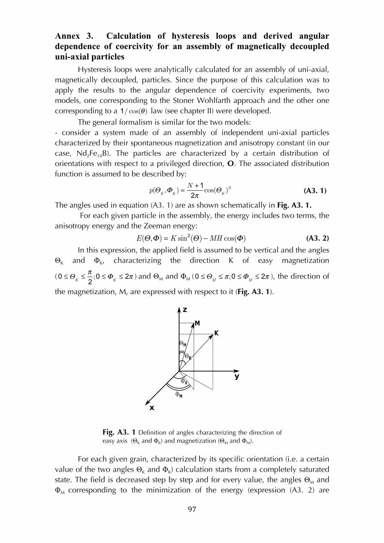
! 97!

Annex 3. Calculation of hysteresis loops and derived angular

dependence of coercivity for an assembly of magnetically decoupled

uni-axial particles

Hysteresis loops were analytically calculated for an assembly of uni-axial,

magnetically decoupled, particles. Since the purpose of this calculation was to

apply the results to the angular dependence of coercivity experiments, two

models, one corresponding to the Stoner Wohlfarth approach and the other one

corresponding to a 1/ cos(θ) law (see chapter II) were developed.

The general formalism is similar for the two models:

- consider a system made of an assembly of independent uni-axial particles

characterized by their spontaneous magnetization and anisotropy constant (in our

case, Nd2Fe14B). The particles are characterized by a certain distribution of

orientations with respect to a privileged direction, O. The associated distribution

function is assumed to be described by:

p(Θ

K,Φ

K) =

N +1

2πcos(Θ

K)N (A3. 1)

The angles used in equation (A3. 1) are as shown schematically in Fig. A3. 1.

For each given particle in the assembly, the energy includes two terms, the

anisotropy energy and the Zeeman energy:

E(Θ,Φ) = K sin2(Θ)−MH cos(Φ) (A3. 2)

In this expression, the applied field is assumed to be vertical and the angles

ΘK and ΦK, characterizing the direction K of easy magnetization

(

0 ≤ΘK≤π

2;0 ≤Φ

K≤ 2π ) and ΘM and ΦM ( 0 ≤Θ

M≤ π;0 ≤Φ

M≤ 2π ), the direction of

the magnetization, M, are expressed with respect to it (Fig. A3. 1).

Fig. A3. 1 Definition of angles characterizing the direction of easy axis (ΘK and ΦK) and magnetization (ΘM and ΦM).

For each given grain, characterized by its specific orientation (i.e. a certain

value of the two angles ΘK and ΦK) calculation starts from a completely saturated

state. The field is decreased step by step and for every value, the angles ΘM and

ΦM corresponding to the minimization of the energy (expression (A3. 2) are

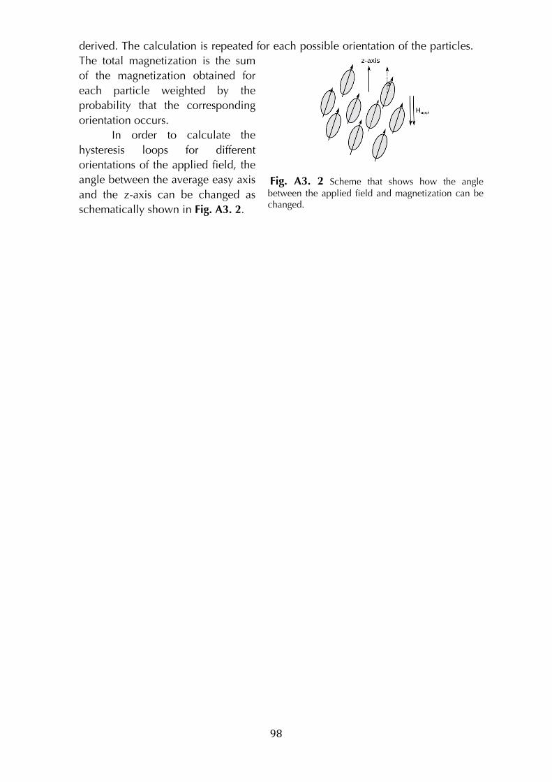
! 98!

derived. The calculation is repeated for each possible orientation of the particles.

The total magnetization is the sum

of the magnetization obtained for

each particle weighted by the

probability that the corresponding

orientation occurs.

In order to calculate the

hysteresis loops for different

orientations of the applied field, the

angle between the average easy axis

and the z-axis can be changed as

schematically shown in Fig. A3. 2.

Fig. A3. 2 Scheme that shows how the angle between the applied field and magnetization can be changed.

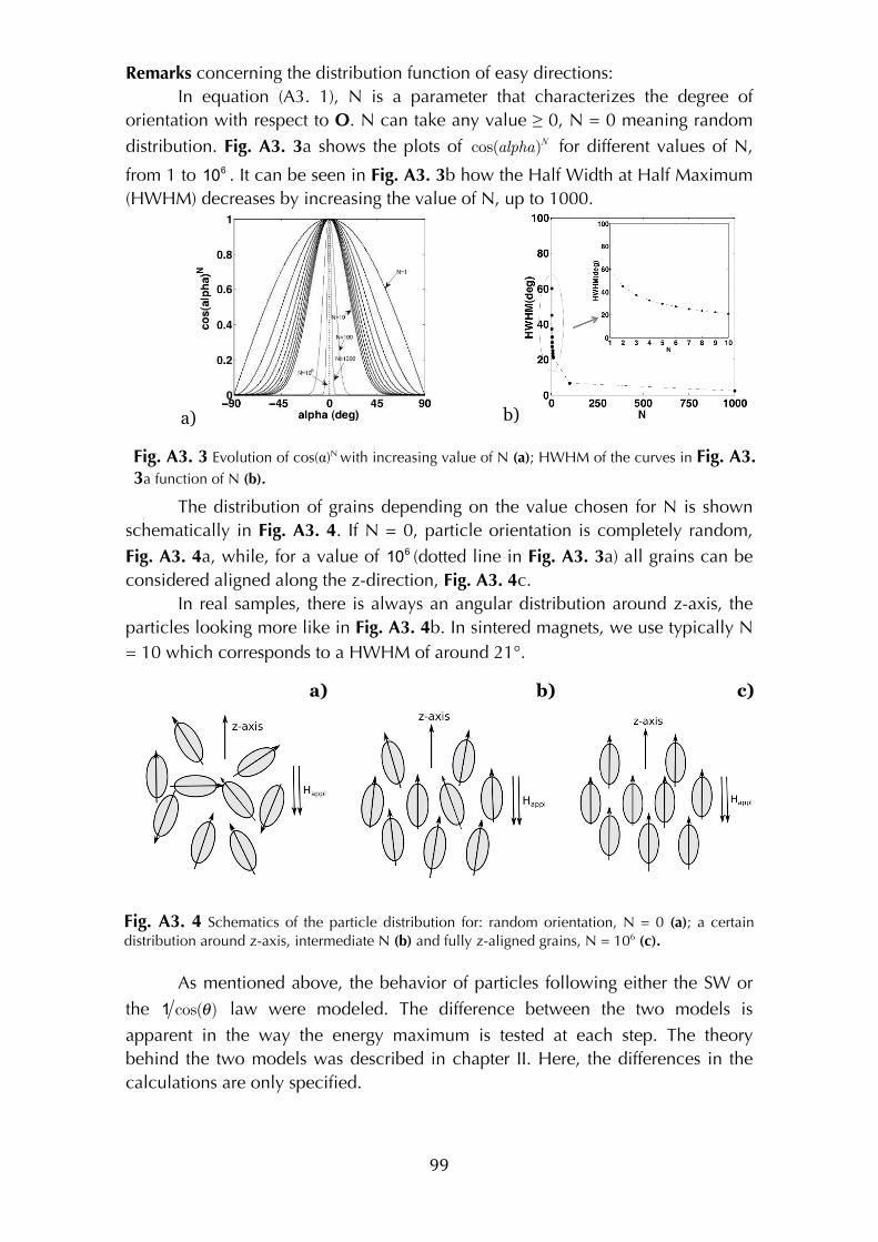
! 99!

Remarks concerning the distribution function of easy directions:

In equation (A3. 1), N is a parameter that characterizes the degree of

orientation with respect to O. N can take any value ≥ 0, N = 0 meaning random

distribution. Fig. A3. 3a shows the plots of cos(alpha)N for different values of N,

from 1 to 106 . It can be seen in Fig. A3. 3b how the Half Width at Half Maximum

(HWHM) decreases by increasing the value of N, up to 1000.

a) b)

Fig. A3. 3 Evolution of cos(α)N with increasing value of N (a); HWHM of the curves in Fig. A3. 3a function of N (b).!

The distribution of grains depending on the value chosen for N is shown

schematically in Fig. A3. 4. If N = 0, particle orientation is completely random,

Fig. A3. 4a, while, for a value of 106 (dotted line in Fig. A3. 3a) all grains can be

considered aligned along the z-direction, Fig. A3. 4c.

In real samples, there is always an angular distribution around z-axis, the

particles looking more like in Fig. A3. 4b. In sintered magnets, we use typically N

= 10 which corresponds to a HWHM of around 21°.

a)

b)

c)

Fig. A3. 4 Schematics of the particle distribution for: random orientation, N = 0 (a); a certain distribution around z-axis, intermediate N (b) and fully z-aligned grains, N = 106 (c).!

As mentioned above, the behavior of particles following either the SW or

the 1 cos(θ) law were modeled. The difference between the two models is

apparent in the way the energy maximum is tested at each step. The theory

behind the two models was described in chapter II. Here, the differences in the

calculations are only specified.

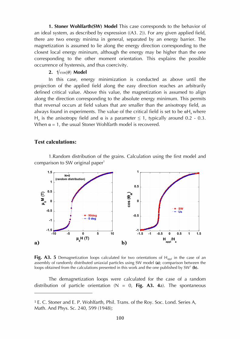
! 100!

1. Stoner Wohlfarth(SW) Model This case corresponds to the behavior of

an ideal system, as described by expression ((A3. 2)). For any given applied field,

there are two energy minima in general, separated by an energy barrier. The

magnetization is assumed to lie along the energy direction corresponding to the

closest local energy mininum, although the energy may be higher than the one

corresponding to the other moment orientation. This explains the possible

occurrence of hysteresis, and thus coercivity.

2. 1 cos(θ) Model

In this case, energy minimization is conducted as above until the

projection of the applied field along the easy direction reaches an arbitrarily

defined critical value. Above this value, the magnetization is assumed to align

along the direction corresponding to the absolute energy minimum. This permits

that reversal occurs at field values that are smaller than the anisotropy field, as

always found in experiments. The value of the critical field is set to be αHa where

Ha is the anisotropy field and α is a parameter ≤ 1, typically around 0.2 - 0.3.

When α = 1, the usual Stoner Wohlfarth model is recovered.

Test calculations:

1.Random distribution of the grains. Calculation using the first model and

comparison to SW original paper1

a)

-1.5

-1

-0.5

0

0.5

1

1.5

-10 -5 0 5 10

90deg0 deg

µ0M

(T

)

µ0H (T)

N=0(random distribution)

b)

-1

-0.5

0

0.5

1

-1.5 -1 -0.5 0 0.5 1 1.5

SWUs

co

s (Θ

M)

Happl

/Ha

Fig. A3. 5 Demagnetization loops calculated for two orientations of Happl in the case of an

assembly of randomly distributed uniaxial particles using SW model (a); comparison between the loops obtained from the calculations presented in this work and the one published by SW1 (b).

The demagnetization loops were calculated for the case of a random

distribution of particle orientation (N = 0, Fig. A3. 4a). The spontaneous

!!!!!!!!!!!!!!!!!!!!!!!!!!!!!!!!!!!!!!!!!!!!!!!!!!!!!!!!

1!E. C. Stoner and E. P. Wohlfarth, Phil. Trans. of the Roy. Soc. Lond. Series A, Math. And Phys. Sc. 240, 599 (1948);!

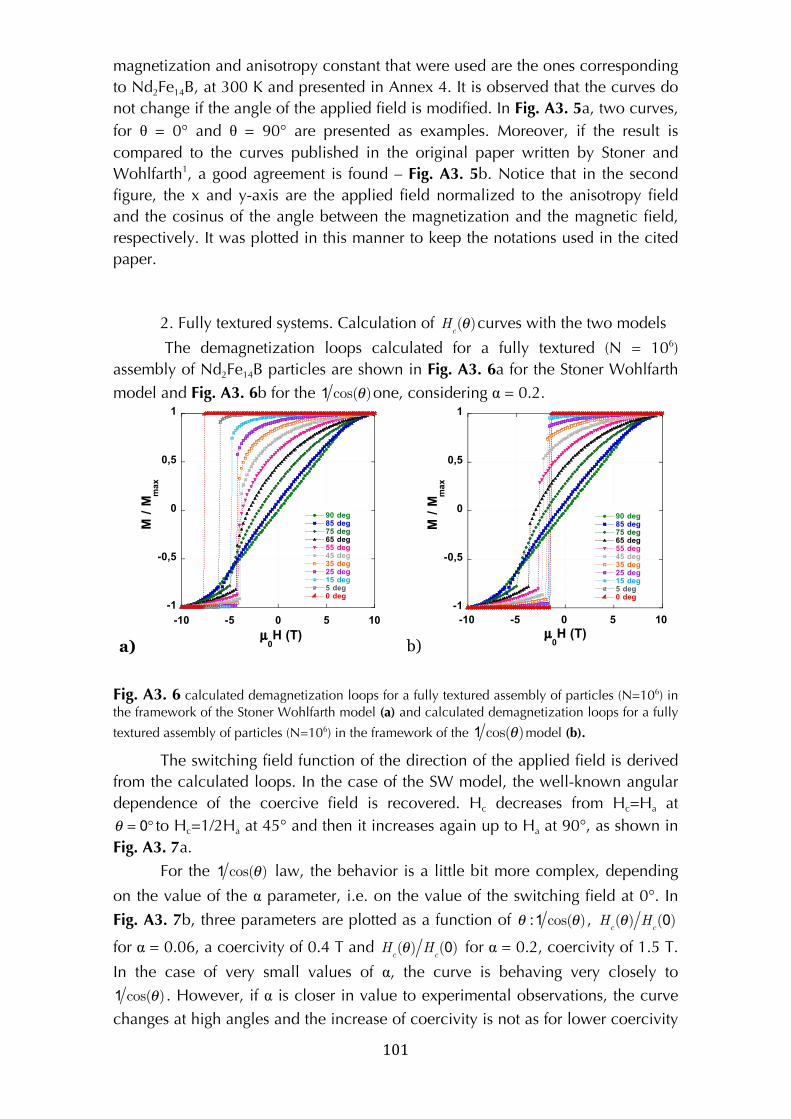
! 101!

magnetization and anisotropy constant that were used are the ones corresponding

to Nd2Fe14B, at 300 K and presented in Annex 4. It is observed that the curves do

not change if the angle of the applied field is modified. In Fig. A3. 5a, two curves,

for θ = 0° and θ = 90° are presented as examples. Moreover, if the result is

compared to the curves published in the original paper written by Stoner and

Wohlfarth1, a good agreement is found – Fig. A3. 5b. Notice that in the second

figure, the x and y-axis are the applied field normalized to the anisotropy field

and the cosinus of the angle between the magnetization and the magnetic field,

respectively. It was plotted in this manner to keep the notations used in the cited

paper.

2. Fully textured systems. Calculation of H

c(θ)curves with the two models

The demagnetization loops calculated for a fully textured (N = 106)

assembly of Nd2Fe14B particles are shown in Fig. A3. 6a for the Stoner Wohlfarth

model and Fig. A3. 6b for the 1 cos(θ)one, considering α = 0.2.

a)

-1

-0,5

0

0,5

1

-10 -5 0 5 10

90 deg85 deg75 deg65 deg55 deg45 deg35 deg25 deg15 deg5 deg0 deg

M /

Mm

ax

µ0H (T)

b)

-1

-0,5

0

0,5

1

-10 -5 0 5 10

90 deg85 deg75 deg65 deg55 deg45 deg35 deg25 deg15 deg5 deg0 deg

µ0H (T)

M /

Mm

ax

Fig. A3. 6 calculated demagnetization loops for a fully textured assembly of particles (N=106) in the framework of the Stoner Wohlfarth model (a) and calculated demagnetization loops for a fully

textured assembly of particles (N=106) in the framework of the 1 cos(θ)model (b).!

The switching field function of the direction of the applied field is derived

from the calculated loops. In the case of the SW model, the well-known angular

dependence of the coercive field is recovered. Hc decreases from Hc=Ha at

θ = 0° to Hc=1/2Ha at 45° and then it increases again up to Ha at 90°, as shown in

Fig. A3. 7a.

For the 1 cos(θ) law, the behavior is a little bit more complex, depending

on the value of the α parameter, i.e. on the value of the switching field at 0°. In

Fig. A3. 7b, three parameters are plotted as a function of θ : 1 cos(θ) , H

c(θ) H

c(0)

for α = 0.06, a coercivity of 0.4 T and H

c(θ) H

c(0) for α = 0.2, coercivity of 1.5 T.

In the case of very small values of α, the curve is behaving very closely to

1 cos(θ) . However, if α is closer in value to experimental observations, the curve

changes at high angles and the increase of coercivity is not as for lower coercivity

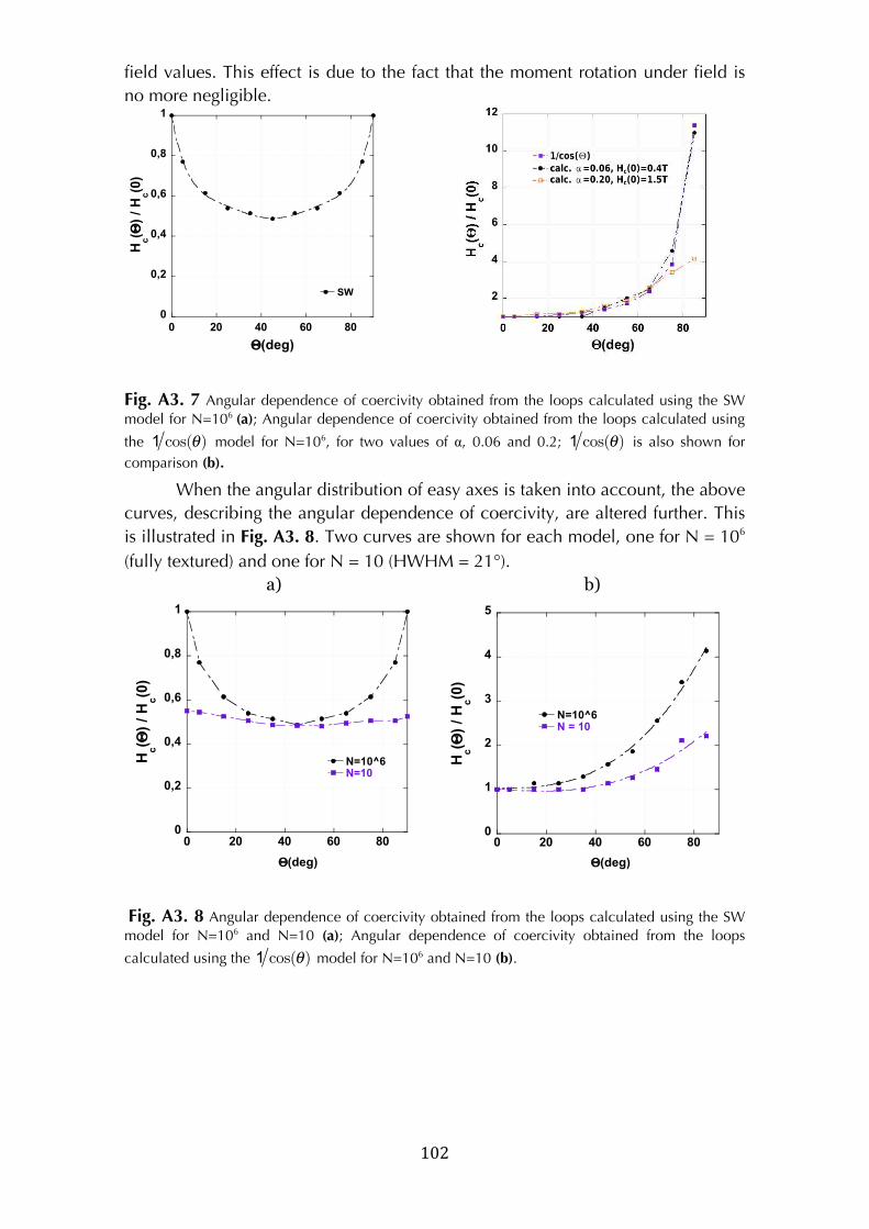
! 102!

field values. This effect is due to the fact that the moment rotation under field is

no more negligible.

0

0,2

0,4

0,6

0,8

1

0 20 40 60 80

SW

Hc(Θ

) /

Hc(0

)

Θ(deg)

Fig. A3. 7 Angular dependence of coercivity obtained from the loops calculated using the SW model for N=106 (a); Angular dependence of coercivity obtained from the loops calculated using

the 1 cos(θ) model for N=106, for two values of α, 0.06 and 0.2; 1 cos(θ) is also shown for

comparison (b).

When the angular distribution of easy axes is taken into account, the above

curves, describing the angular dependence of coercivity, are altered further. This

is illustrated in Fig. A3. 8. Two curves are shown for each model, one for N = 106

(fully textured) and one for N = 10 (HWHM = 21°).

a)

0

0,2

0,4

0,6

0,8

1

0 20 40 60 80

N=10^6N=10

Hc(Θ

) /

Hc(0

)

Θ(deg)

b)

0

1

2

3

4

5

0 20 40 60 80

N=10^6N = 10

Θ(deg)

Hc(Θ

) /

Hc(0

)

Fig. A3. 8 Angular dependence of coercivity obtained from the loops calculated using the SW model for N=106 and N=10 (a); Angular dependence of coercivity obtained from the loops

calculated using the 1 cos(θ) model for N=106 and N=10 (b).!

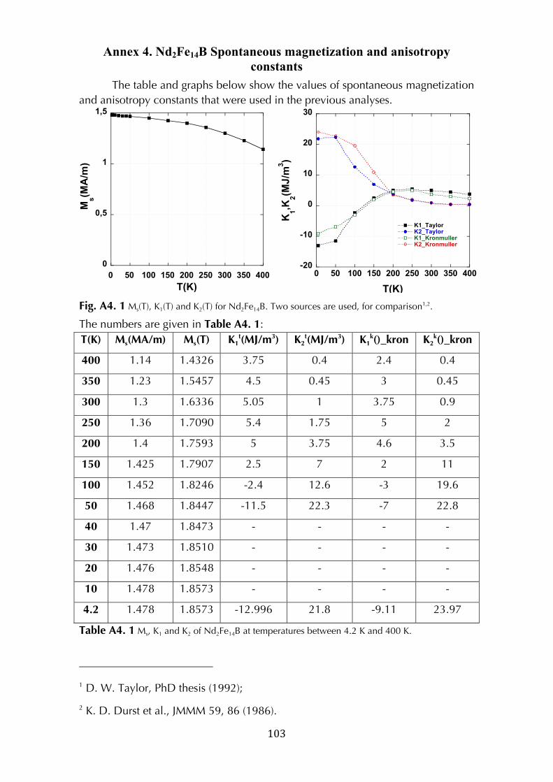
! 103!

Annex 4. Nd2Fe14B Spontaneous magnetization and anisotropy

constants

The table and graphs below show the values of spontaneous magnetization

and anisotropy constants that were used in the previous analyses.

0

0,5

1

1,5

0 50 100 150 200 250 300 350 400

Ms(MA/m)

T(K)

-20

-10

0

10

20

30

0 50 100 150 200 250 300 350 400

K1_TaylorK2_TaylorK1_KronmullerK2_Kronmuller

K1,K

2(M

J/m

3)

T(K)

Fig. A4. 1 Ms(T), K1(T) and K2(T) for Nd2Fe14B. Two sources are used, for comparison1,2.

The numbers are given in Table A4. 1:

T(K) Ms(MA/m) Ms(T) K1t(MJ/m3) K2

t(MJ/m3) K1k()_kron K2

k()_kron

400 1.14 1.4326 3.75 0.4 2.4 0.4

350 1.23 1.5457 4.5 0.45 3 0.45

300 1.3 1.6336 5.05 1 3.75 0.9

250 1.36 1.7090 5.4 1.75 5 2

200 1.4 1.7593 5 3.75 4.6 3.5

150 1.425 1.7907 2.5 7 2 11

100 1.452 1.8246 -2.4 12.6 -3 19.6

50 1.468 1.8447 -11.5 22.3 -7 22.8

40 1.47 1.8473 - - - -

30 1.473 1.8510 - - - -

20 1.476 1.8548 - - - -

10 1.478 1.8573 - - - -

4.2 1.478 1.8573 -12.996 21.8 -9.11 23.97

Table A4. 1 Ms, K1 and K2 of Nd2Fe14B at temperatures between 4.2 K and 400 K.

!!!!!!!!!!!!!!!!!!!!!!!!!!!!!!!!!!!!!!!!!!!!!!!!!!!!!!!!

1 D. W. Taylor, PhD thesis (1992);

2 K. D. Durst et al., JMMM 59, 86 (1986).

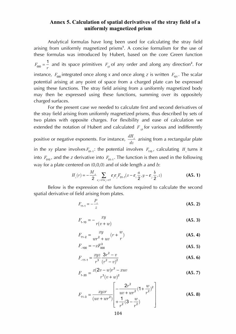
! 104!

Annex 5. Calculation of spatial derivatives of the stray field of a

uniformly magnetized prism

Analytical formulas have long been used for calculating the stray field

arising from uniformly magnetized prisms1. A concise formalism for the use of

these formulas was introduced by Hubert, based on the core Green function

F000

=1

r and its space primitives

F

ijkof any order and along any direction2. For

instance, F

000integrated once along x and once along z is written

F

101. The scalar

potential arising at any point of space from a charged plate can be expressed

using these functions. The stray field arising from a uniformly magnetized body

may then be expressed using these functions, summing over its oppositely

charged surfaces.

For the present case we needed to calculate first and second derivatives of

the stray field arising from uniformly magnetized prisms, thus described by sets of

two plates with opposite charges. For flexibility and ease of calculation we

extended the notation of Hubert and calculated F

ijkfor various and indifferently

positive or negative exponents. For instance,

dHx

dz arising from a rectangular plate

in the xy plane involves F

01−1: the potential involves

F

110, calculating

H

zturns it

into F

010, and the z derivative into

F

01−1. The function is then used in the following

way for a plate centered on (0,0,0) and of side length a and b:

Hz(r) = −

Ms

2ε

iε

jF

01−1

εi=±1;ε

j=±1

∑ (x − εi

a

2,y − ε

j

b

2,z) (A5. 1)

Below is the expression of the functions required to calculate the second

spatial derivative of field arising from plates.

F11−1

= −P

z

z (A5. 2)

(A5. 3)

(A5. 4)

(A5. 5)

F

−11−1=

xyz

r3

3r2− v

(r 2− v)2

(A5. 6)

(A5. 7)

F11−3

=xyzr

(uv +wr2)

−2r

2

uv +wr2(1+

w

r2)2

+1

r2(3 −

w

r2)

⎡

⎣

⎢⎢⎢⎢

⎤

⎦

⎥⎥⎥⎥

(A5. 8)

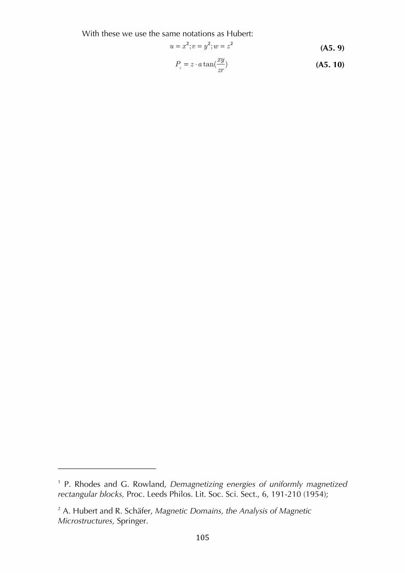
! 105!

With these we use the same notations as Hubert:

u = x

2;v = y

2;w = z

2 (A5. 9)

P

z= z ⋅a tan(

xy

zr) (A5. 10)

!

!

!

!

!

!

!

!

!

!

!

!

!

!

!

!

!

!

!

!

!

!

!

!!!!!!!!!!!!!!!!!!!!!!!!!!!!!!!!!!!!!!!!!!!!!!!!!!!!!!!!

1 P. Rhodes and G. Rowland, Demagnetizing energies of uniformly magnetized rectangular blocks, Proc. Leeds Philos. Lit. Soc. Sci. Sect., 6, 191-210 (1954);

2 A. Hubert and R. Schäfer, Magnetic Domains, the Analysis of Magnetic Microstructures, Springer.!

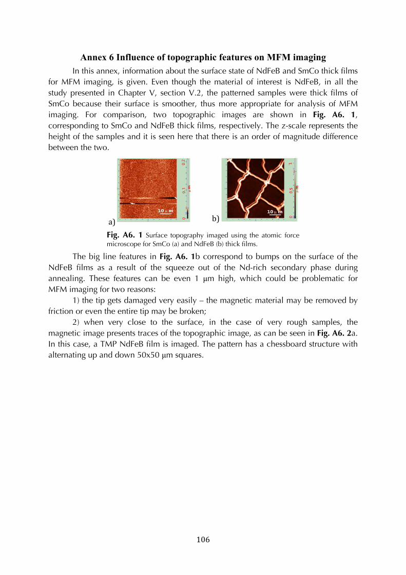
! 106!

Annex 6 Influence of topographic features on MFM imaging

In this annex, information about the surface state of NdFeB and SmCo thick films

for MFM imaging, is given. Even though the material of interest is NdFeB, in all the

study presented in Chapter V, section V.2, the patterned samples were thick films of

SmCo because their surface is smoother, thus more appropriate for analysis of MFM

imaging. For comparison, two topographic images are shown in Fig. A6. 1,

corresponding to SmCo and NdFeB thick films, respectively. The z-scale represents the

height of the samples and it is seen here that there is an order of magnitude difference

between the two.

a)! ! b)! !

Fig. A6. 1 Surface topography imaged using the atomic force microscope for SmCo (a) and NdFeB (b) thick films.

The big line features in Fig. A6. 1b correspond to bumps on the surface of the

NdFeB films as a result of the squeeze out of the Nd-rich secondary phase during

annealing. These features can be even 1 µm high, which could be problematic for

MFM imaging for two reasons:

1) the tip gets damaged very easily – the magnetic material may be removed by

friction or even the entire tip may be broken;

2) when very close to the surface, in the case of very rough samples, the

magnetic image presents traces of the topographic image, as can be seen in Fig. A6. 2a.

In this case, a TMP NdFeB film is imaged. The pattern has a chessboard structure with

alternating up and down 50x50 µm squares.

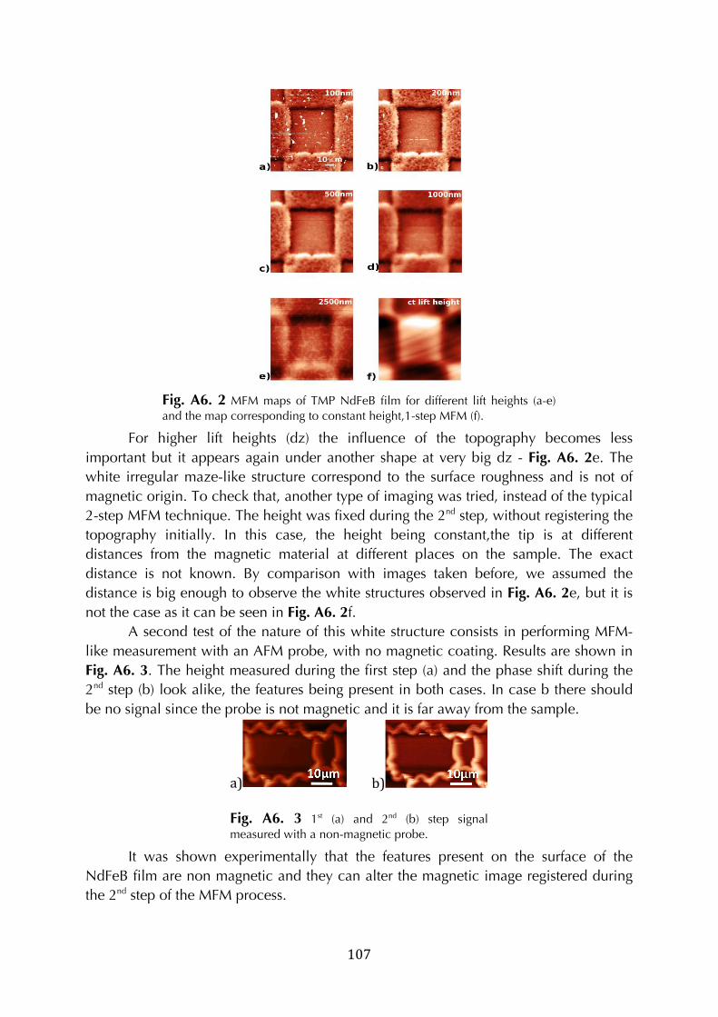
! 107!

Fig. A6. 2 MFM maps of TMP NdFeB film for different lift heights (a-e) and the map corresponding to constant height,1-step MFM (f).

For higher lift heights (dz) the influence of the topography becomes less

important but it appears again under another shape at very big dz - Fig. A6. 2e. The

white irregular maze-like structure correspond to the surface roughness and is not of

magnetic origin. To check that, another type of imaging was tried, instead of the typical

2-step MFM technique. The height was fixed during the 2nd step, without registering the

topography initially. In this case, the height being constant,the tip is at different

distances from the magnetic material at different places on the sample. The exact

distance is not known. By comparison with images taken before, we assumed the

distance is big enough to observe the white structures observed in Fig. A6. 2e, but it is

not the case as it can be seen in Fig. A6. 2f.

A second test of the nature of this white structure consists in performing MFM-

like measurement with an AFM probe, with no magnetic coating. Results are shown in

Fig. A6. 3. The height measured during the first step (a) and the phase shift during the

2nd step (b) look alike, the features being present in both cases. In case b there should

be no signal since the probe is not magnetic and it is far away from the sample.

a) ! b) !

Fig. A6. 3 1st (a) and 2nd (b) step signal measured with a non-magnetic probe.

It was shown experimentally that the features present on the surface of the

NdFeB film are non magnetic and they can alter the magnetic image registered during

the 2nd step of the MFM process.

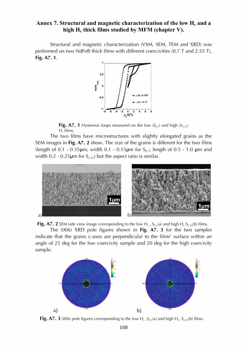
! 108!

Annex 7. Structural and magnetic characterization of the low Hc and a

high Hc thick films studied by MFM (chapter V).

!

Structural and magnetic characterization (VSM, SEM, TEM and XRD) was

performed on two NdFeB thick films with different coercivities (0.7 T and 2.55 T),

Fig. A7. 1.

!

Fig. A7. 1 Hysteresis loops measured on the low (S0.7) and high (S2.55) Hc films.

The two films have microstructures with slightly elongated grains as the

SEM images in Fig. A7. 2 show. The size of the grains is different for the two films

(length of 0.1 - 0.35μm, width 0.1 - 0.15μm for S0.7; length of 0.5 - 1.0 μm and

width 0.2 - 0.25μm for S2.55) but the aspect ratio is similar.

a) b)

Fig. A7. 2 SEM side view image corresponding to the low Hc , S0.7(a) and high Hc S2.55(b) films.

The (006) XRD pole figures shown in Fig. A7. 3 for the two samples

indicate that the grains c-axes are perpendicular to the films’ surface within an

angle of 25 deg for the low coercivity sample and 20 deg for the high coercivity

sample.

a) ! b) !

Fig. A7. 3 (006) pole figures corresponding to the low Hc ,S0.7(a) and high Hc, S2.55(b) films.

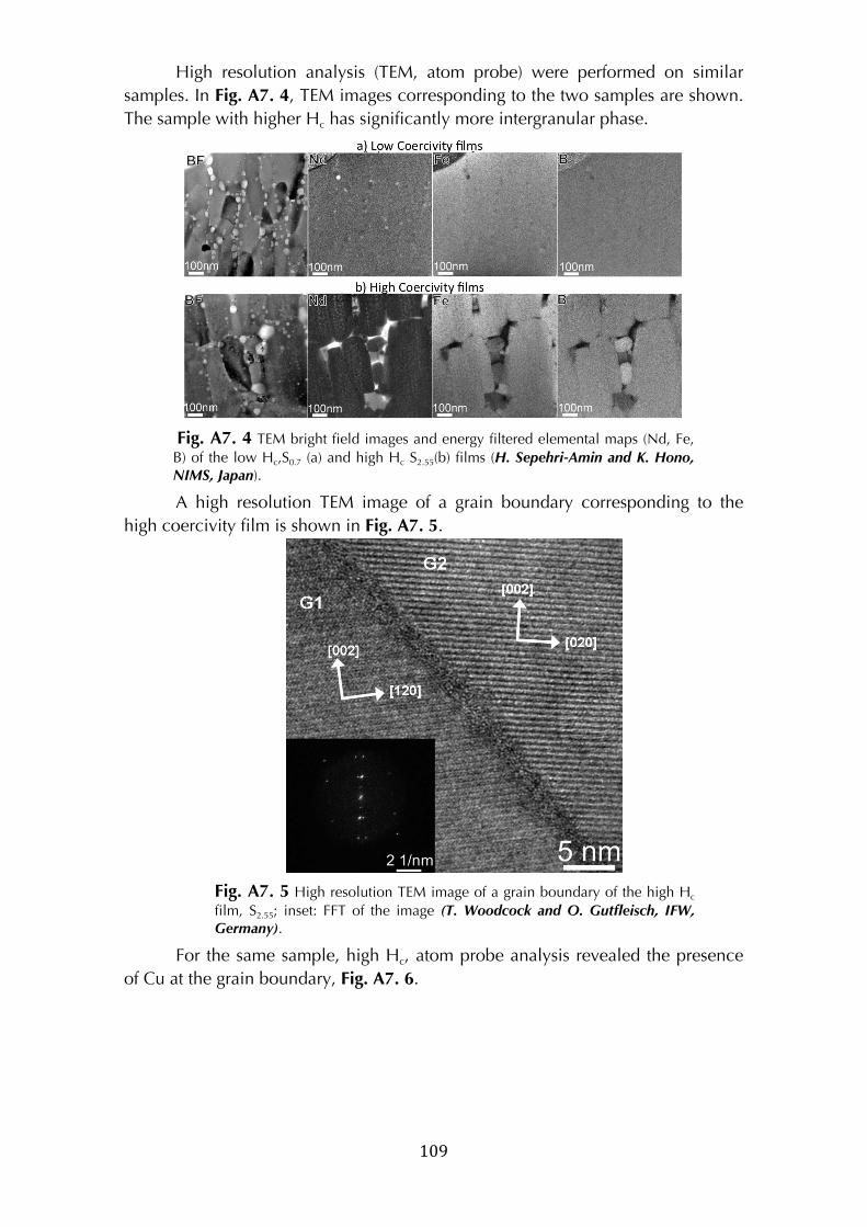
! 109!

High resolution analysis (TEM, atom probe) were performed on similar

samples. In Fig. A7. 4, TEM images corresponding to the two samples are shown.

The sample with higher Hc has significantly more intergranular phase.

!

Fig. A7. 4 TEM bright field images and energy filtered elemental maps (Nd, Fe, B) of the low Hc,S0.7 (a) and high Hc S2.55(b) films (H. Sepehri-Amin and K. Hono, NIMS, Japan).

A high resolution TEM image of a grain boundary corresponding to the

high coercivity film is shown in Fig. A7. 5.

!

Fig. A7. 5 High resolution TEM image of a grain boundary of the high Hc film, S2.55; inset: FFT of the image (T. Woodcock and O. Gutfleisch, IFW, Germany).

For the same sample, high Hc, atom probe analysis revealed the presence

of Cu at the grain boundary, Fig. A7. 6.

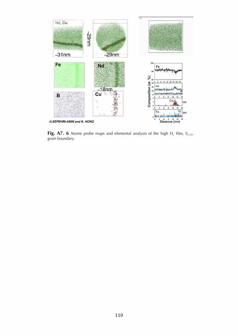
! 110!

!

Fig. A7. 6 Atome probe maps and elemental analysis of the high Hc film, S2.55, grain boundary.

!

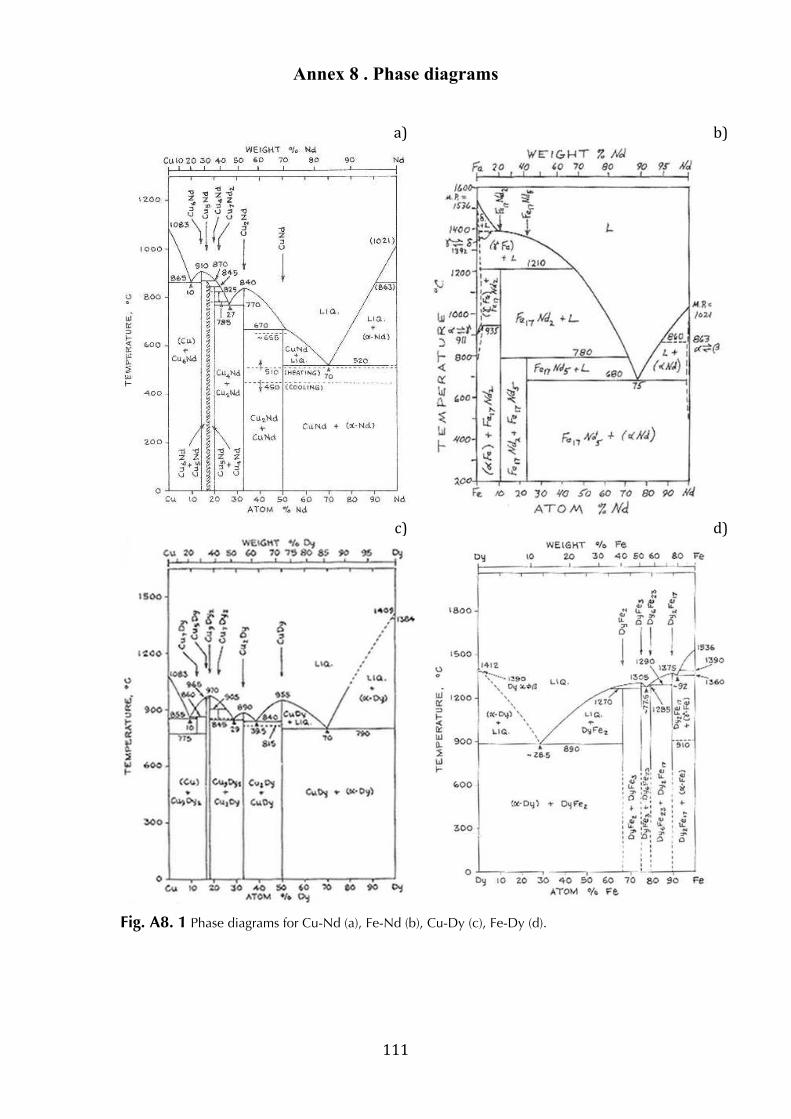
! 111!

Annex 8 . Phase diagrams

!

a)

!

b)

!c)

!

d)

!

Fig. A8. 1 Phase diagrams for Cu-Nd (a), Fe-Nd (b), Cu-Dy (c), Fe-Dy (d).

!

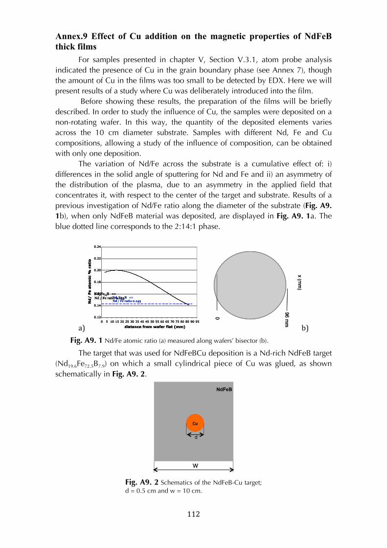
! 112!

Annex.9 Effect of Cu addition on the magnetic properties of NdFeB

thick films

For samples presented in chapter V, Section V.3.1, atom probe analysis

indicated the presence of Cu in the grain boundary phase (see Annex 7), though

the amount of Cu in the films was too small to be detected by EDX. Here we will

present results of a study where Cu was deliberately introduced into the film.

Before showing these results, the preparation of the films will be briefly

described. In order to study the influence of Cu, the samples were deposited on a

non-rotating wafer. In this way, the quantity of the deposited elements varies

across the 10 cm diameter substrate. Samples with different Nd, Fe and Cu

compositions, allowing a study of the influence of composition, can be obtained

with only one deposition.

The variation of Nd/Fe across the substrate is a cumulative effect of: i)

differences in the solid angle of sputtering for Nd and Fe and ii) an asymmetry of

the distribution of the plasma, due to an asymmetry in the applied field that

concentrates it, with respect to the center of the target and substrate. Results of a

previous investigation of Nd/Fe ratio along the diameter of the substrate (Fig. A9.

1b), when only NdFeB material was deposited, are displayed in Fig. A9. 1a. The

blue dotted line corresponds to the 2:14:1 phase.

a)! ! b)!!

Fig. A9. 1 Nd/Fe atomic ratio (a) measured along wafers’ bisector (b).

The target that was used for NdFeBCu deposition is a Nd-rich NdFeB target

(Nd19.6Fe72.5B7.9) on which a small cylindrical piece of Cu was glued, as shown

schematically in Fig. A9. 2.

!

Fig. A9. 2 Schematics of the NdFeB-Cu target; d = 0.5 cm and w = 10 cm.

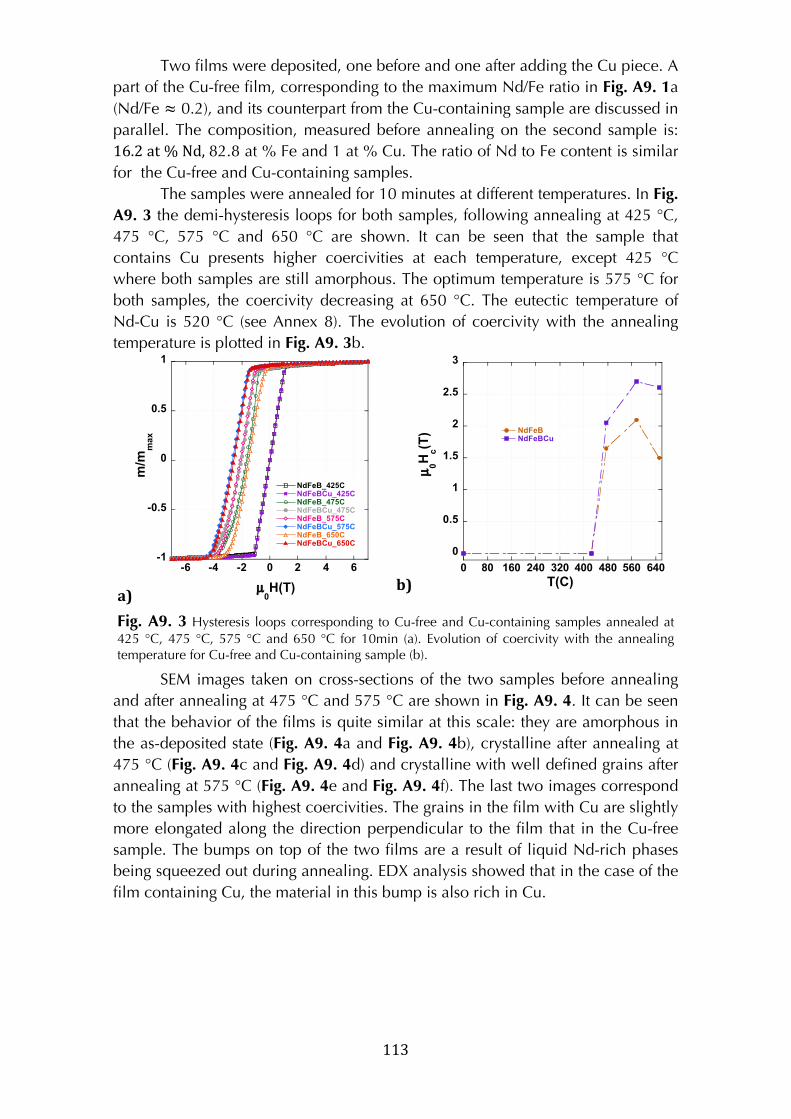
! 113!

Two films were deposited, one before and one after adding the Cu piece. A

part of the Cu-free film, corresponding to the maximum Nd/Fe ratio in Fig. A9. 1a

(Nd/Fe ≈ 0.2), and its counterpart from the Cu-containing sample are discussed in

parallel. The composition, measured before annealing on the second sample is:

16.2!at!%!Nd,!82.8 at % Fe and 1 at % Cu. The ratio of Nd to Fe content is similar

for the Cu-free and Cu-containing samples.

The samples were annealed for 10 minutes at different temperatures. In Fig.

A9. 3 the demi-hysteresis loops for both samples, following annealing at 425 °C,

475 °C, 575 °C and 650 °C are shown. It can be seen that the sample that

contains Cu presents higher coercivities at each temperature, except 425 °C

where both samples are still amorphous. The optimum temperature is 575 °C for

both samples, the coercivity decreasing at 650 °C. The eutectic temperature of

Nd-Cu is 520 °C (see Annex 8). The evolution of coercivity with the annealing

temperature is plotted in Fig. A9. 3b.

a)

-1

-0.5

0

0.5

1

-6 -4 -2 0 2 4 6

NdFeB_425CNdFeBCu_425CNdFeB_475CNdFeBCu_475CNdFeB_575CNdFeBCu_575CNdFeB_650CNdFeBCu_650C

m/m

max

µ0H(T)

#b)!

0

0.5

1

1.5

2

2.5

3

0 80 160 240 320 400 480 560 640

NdFeBNdFeBCu

µ0Hc(T)

T(C) #!

Fig. A9. 3 Hysteresis loops corresponding to Cu-free and Cu-containing samples annealed at 425 °C, 475 °C, 575 °C and 650 °C for 10min (a). Evolution of coercivity with the annealing temperature for Cu-free and Cu-containing sample (b).

SEM images taken on cross-sections of the two samples before annealing

and after annealing at 475 °C and 575 °C are shown in Fig. A9. 4. It can be seen

that the behavior of the films is quite similar at this scale: they are amorphous in

the as-deposited state (Fig. A9. 4a and Fig. A9. 4b), crystalline after annealing at

475 °C (Fig. A9. 4c and Fig. A9. 4d) and crystalline with well defined grains after

annealing at 575 °C (Fig. A9. 4e and Fig. A9. 4f). The last two images correspond

to the samples with highest coercivities. The grains in the film with Cu are slightly

more elongated along the direction perpendicular to the film that in the Cu-free

sample. The bumps on top of the two films are a result of liquid Nd-rich phases

being squeezed out during annealing. EDX analysis showed that in the case of the

film containing Cu, the material in this bump is also rich in Cu.

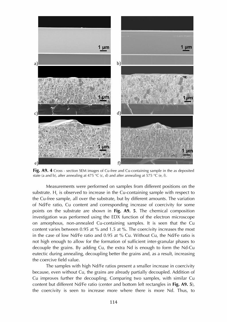
! 114!

a) ! b) !

c) ! d) !

e) ! f) !

Fig. A9. 4 Cross - section SEM images of Cu-free and Cu-containing sample in the as deposited state (a and b), after annealing at 475 °C (c, d) and after annealing at 575 °C (e, f).

Measurements were performed on samples from different positions on the

substrate. Hc is observed to increase in the Cu-containing sample with respect to

the Cu-free sample, all over the substrate, but by different amounts. The variation

of Nd/Fe ratio, Cu content and corresponding increase of coercivity for some

points on the substrate are shown in Fig. A9. 5. The chemical composition

investigation was performed using the EDX function of the electron microscope

on amorphous, non-annealed Cu-containing samples. It is seen that the Cu

content varies between 0.95 at % and 1.5 at %. The coercivity increases the most

in the case of low Nd/Fe ratio and 0.95 at % Cu. Without Cu, the Nd/Fe ratio is

not high enough to allow for the formation of sufficient inter-granular phases to

decouple the grains. By adding Cu, the extra Nd is enough to form the Nd-Cu

eutectic during annealing, decoupling better the grains and, as a result, increasing

the coercive field value.

The samples with high Nd/Fe ratios present a smaller increase in coercivity

because, even without Cu, the grains are already partially decoupled. Addition of

Cu improves further the decoupling. Comparing two samples, with similar Cu

content but different Nd/Fe ratio (center and bottom left rectangles in Fig. A9. 5),

the coercivity is seen to increase more where there is more Nd. Thus, to

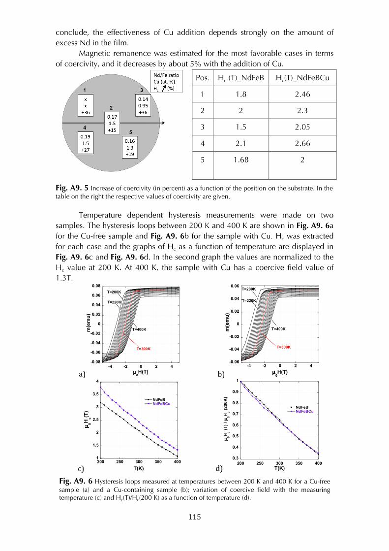
! 115!

conclude, the effectiveness of Cu addition depends strongly on the amount of

excess Nd in the film.

Magnetic remanence was estimated for the most favorable cases in terms

of coercivity, and it decreases by about 5% with the addition of Cu.

Pos. Hc (T)_NdFeB Hc(T)_NdFeBCu

1 1.8 2.46

2 2 2.3

3 1.5 2.05

4 2.1 2.66

5 1.68 2

Fig. A9. 5 Increase of coercivity (in percent) as a function of the position on the substrate. In the table on the right the respective values of coercivity are given.

Temperature dependent hysteresis measurements were made on two

samples. The hysteresis loops between 200 K and 400 K are shown in Fig. A9. 6a

for the Cu-free sample and Fig. A9. 6b for the sample with Cu. Hc was extracted

for each case and the graphs of Hc as a function of temperature are displayed in

Fig. A9. 6c and Fig. A9. 6d. In the second graph the values are normalized to the

Hc value at 200 K. At 400 K, the sample with Cu has a coercive field value of

1.3T.

a)

-0.08

-0.06

-0.04

-0.02

0

0.02

0.04

0.06

0.08

-4 -2 0 2 4

T=200K

T=220K

T=400K

T=300K

µ0H(T)

m(emu)

! b)

-0.06

-0.04

-0.02

0

0.02

0.04

0.06

-4 -2 0 2 4

m(emu)

µ0H(T)

T=400K

T=200K

T=220K

T=300K

!

c)

1

1.5

2

2.5

3

3.5

4

200 250 300 350 400

NdFeBNdFeBCu

µ0Hc(T)

T(K) ! d)

0.3

0.4

0.5

0.6

0.7

0.8

0.9

1

200 250 300 350 400

NdFeBNdFeBCu

µ0H

c (

T)

/ µ

0H

c (

200K

)

T(K) !

Fig. A9. 6 Hysteresis loops measured at temperatures between 200 K and 400 K for a Cu-free sample (a) and a Cu-containing sample (b); variation of coercive field with the measuring temperature (c) and Hc(T)/Hc(200 K) as a function of temperature (d).

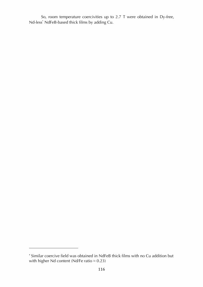
! 116!

So, room temperature coercivities up to 2.7 T were obtained in Dy-free,

Nd-less* NdFeB-based thick films by adding Cu.

!

!

!!!!!!!!!!!!!!!!!!!!!!!!!!!!!!!!!!!!!!!!!!!!!!!!!!!!!!!!

*!Similar coercive field was obtained in NdFeB thick films with no Cu addition but with higher Nd content (Nd/Fe ratio ≈ 0.23)!

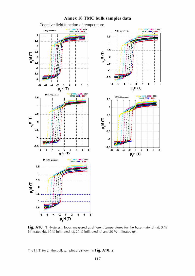
! 117!

Annex 10 TMC bulk samples data

Coercive field function of temperature

! !

-1,5

-1

-0,5

0

0,5

1

1,5

-8 -6 -4 -2 0 2 4 6 8

M(H) 20percent

µ0H (T)

µ0M

(T

)

100K; 150K; 200K; 250K 300K; 350K; 400K

!

!

!

Fig. A10. 1 Hysteresis loops measured at different temperatures for the base material (a), 5 % infiltrated (b), 10 % infiltrated (c), 20 % infiltrated (d) and 30 % infiltrated (e).

!

!

The Hc(T) for all the bulk samples are shown in Fig. A10. 2.

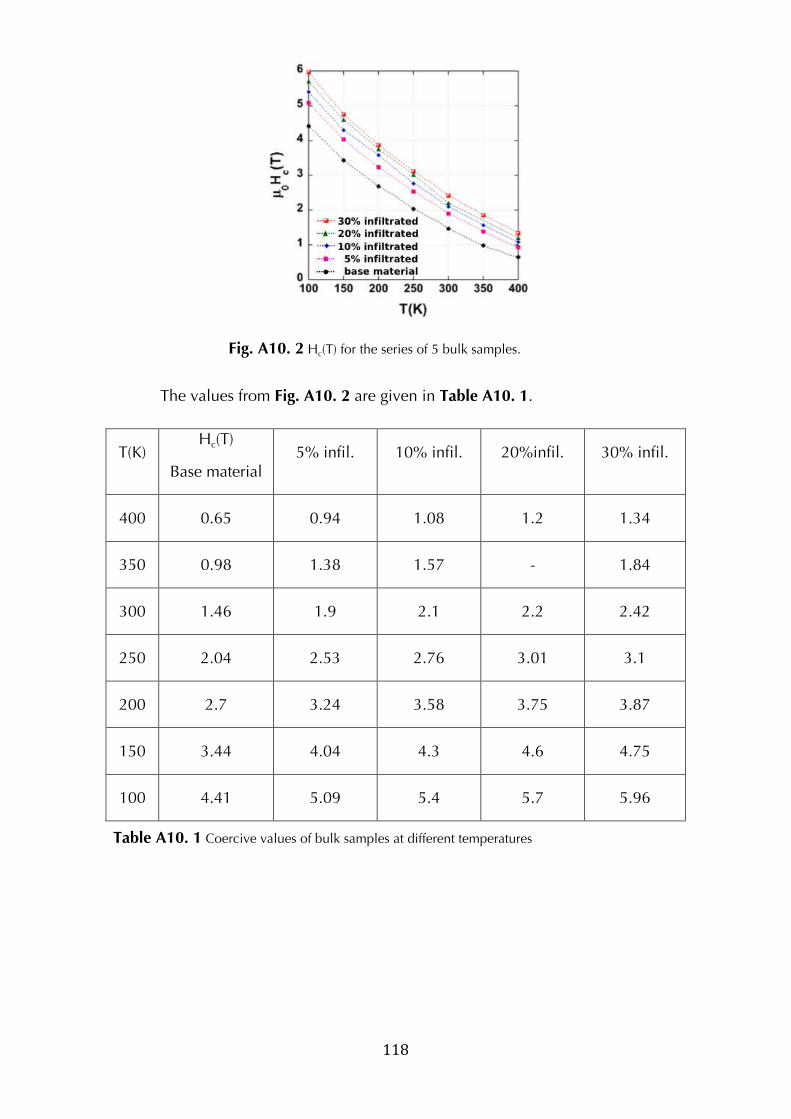
! 118!

!

Fig. A10. 2 Hc(T) for the series of 5 bulk samples.

The values from Fig. A10. 2 are given in Table A10. 1.

T(K) Hc(T)

Base material 5% infil. 10% infil. 20%infil. 30% infil.

400 0.65 0.94 1.08 1.2 1.34

350 0.98 1.38 1.57 - 1.84

300 1.46 1.9 2.1 2.2 2.42

250 2.04 2.53 2.76 3.01 3.1

200 2.7 3.24 3.58 3.75 3.87

150 3.44 4.04 4.3 4.6 4.75

100 4.41 5.09 5.4 5.7 5.96

Table A10. 1 Coercive values of bulk samples at different temperatures !

!

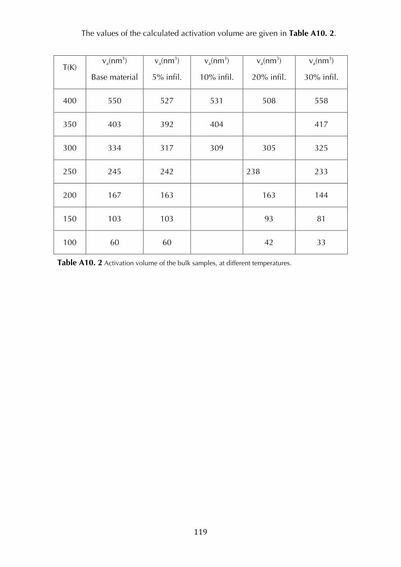
! 119!

The values of the calculated activation volume are given in Table A10. 2.

!

T(K) va(nm3)

Base material

va(nm3)

5% infil.

va(nm3)

10% infil.

va(nm3)

20% infil.

va(nm3)

30% infil.

400 550 527 531 508 558

350 403 392 404 417

300 334 317 309 305 325

250 245 242 238 233

200 167 163 163 144

150 103 103 93 81

100 60 60 42 33

Table A10. 2 Activation volume of the bulk samples, at different temperatures. !

!

!

Abstract Magnetization reversal in NdFeB-type permanent magnets was studied in this thesis, based on both global (magnetometry) and local (magnetic force microscopy) experimental techniques. Two types of samples were analyzed: bulk magnets of which magnetic properties are greatly improved as a result of NdCu infiltration along the grain boundaries (samples provided by Toyota Motor Corporation) and thick film magnets with different microstructures and thus different coercive fields. The temperature dependence of the coercive field and that of the activation volume were analyzed in the framework of two models: the micromagnetic and the global model. The derived values of the two main parameters characterizing coercivity (N representing demagnetizing field

effects and α linking the coercive field to the intrinsic magnetic properties of the hard phase) indicate that, in bulk magnets, the difference in coercivity between different samples is related

mainly to N whereas in films the parameter α plays the leading role. The activation volume derived from magnetic after effect measurements is similar for all bulk samples at a given temperature. On the opposite, it varies in the case of films: the higher the coercive field, the smaller the activation volume. Altogether, it is concluded that the magnetic properties within the activation volume are close to those of the main phase. The link between microstructure and coercivity was studied in thick films, using magnetic force microscopy. Imaging of films that present different microstructures was performed in different remanent states along the hysteresis cycle. Interaction domains were observed in the case of films with lower coercive field. In such low coercivity films, as well as in medium coercivity ones, magnetization reversal is dominated by domain wall propagation, instead of nucleation + propagation in high coercivity films. Keywords: hard magnetic materials, coercivity, microstructure, magnetization reversal, interaction domains, micromagnetic model, global model, magnetic force microscopy (MFM). Résumé Les processus d’aimantation dans des aimants de type NdFeB ont été étudiés dans le cadre de cette thèse, sur la base de mesures d’aimantation macroscopiques et de caractérisations locales (MFM). Deux types d’échantillons ont été analysés : des aimants massifs dont les propriétés excellentes résultent d’un processus d’infiltration de NdCu le long des joints de grain (échantillons fournis par Toyota Motor Corporation) et des échantillons sous forme de couches épaisses, dont les microstructures, et, de ce fait les propriétés magnétiques, diffèrent. La variation thermique du champ coercitif et celle du volume d’activation ont été analysées dans le cadre de deux modèles, respectivement dénommé micromagnétique et global. Les valeurs déduites des deux paramètres principaux caractérisant la coercitivité (N représentant les effets du champ démagnétisant et

α reliant le champ coercitif aux propriétés magnétiques intrinsèques de la phase dure) indiquent que dans les aimants massifs les différences de coercitivité entre échantillons sont dues pour

l’essentiel à la variation de N alors que dans les films, c’est la variation du paramètre α qui joue le rôle principal. Le volume d’activation à une température donnée, dérivé de mesures de trainage magnétique, a des valeurs proches pour tous les échantillons massifs. Au contraire, il varie d’un échantillon à l’autre dans le cas des films : plus le champ coercitif est fort, plus petit est le volume d’activation. Une conclusion générale de cette étude est que les propriétés magnétiques au sein du volume d’activation sont proches de celles de la phase dure Nd2Fe14B. Le lien entre microstructure et coercivité a été examiné dans les films épais par microscopie de force magnétique (MFM). Des observations de films dans différents états rémanents le long du cycle d’hystérésis ont été réalisées. Des « domaines d’interactions » ont été révélés dans les films de faible coercitivté. Dans de tels films, comme dans ceux de coercitivité moyenne, le renversement d’aimantation est dominé par la propagation de domaines, alors que dans les films de plus forte coercitivité, la nucléation suivie de la propagation de domaines d’orientation inverse à celle de l’aimantation principale dominent. Mots-clés : matériaux magnétiques durs, coercitivité, microstructure, renversement d’aimantation, domaines d’interaction, modèle micromagnétique, modèle global, microscopie de force magnétiques (MFM). !