Understanding Factors Affecting Arterial Reliability ...

Understanding Factors Affecting Arterial Reliability Performance Metrics

Final Report 1117August 2019

Avinash Unnikrishnan, Ph.D.

Sirisha Kothuri, Ph.D.

Jason Anderson, Ph.D.

NATIONAL INSTITUTE FOR TRANSPORTATION AND COMMUNITIES nitc-utc.net

UNDERSTANDING FACTORS AFFECTING ARTERIAL RELIABILITY PERFORMANCE METRICS

Final Report

NITC-RR-1117

by

Jason C. Anderson Rohan Sirupa Sirisha Kothuri

Avinash Unnikrishnan Portland State University

for

National Institute for Transportation and Communities (NITC) P.O. Box 751

Portland, OR 97207

August 2019

i

Technical Report Documentation Page 1. Report No.

NITC-RR-1117

2. Government Accession No.

3. Recipient’s Catalog No.

4. Title and Subtitle Understanding Factors Affecting Arterial Reliability Performance Metrics

5. Report Date Augusts 2019

6. Performing Organization Code

7. Author(s)

Jason C. Anderson, Rohan Sirupa, Sirisha Kothuri, Avinash Unnikrishnan

8. Performing Organization Report No.

9. Performing Organization Name and Address Portland State University Portland, OR 97201

10. Work Unit No. (TRAIS)

11. Contract or Grant No.

12. Sponsoring Agency Name and Address National Institute for Transportation and Communities (NITC) P.O. Box 751 Portland, OR 97207

13. Type of Report and Period Covered

14. Sponsoring Agency Code

15. Supplementary Notes

16. Abstract In recent years, the importance of travel time reliability has become equally important as average travel time. However, the majority focus of travel time research is average travel time or travel time reliability on freeways. In addition, the identification of specific factors (i.e., peak hours, nighttime hours, etc.) and their effects on average travel time and travel time variability are often unknown. The current study addresses these two issues through a travel time-based study on urban arterials. Using travel times collected via Bluetooth data, a series of analyses are conducted to understand factors affecting reliability metrics on urban arterials. Analyses include outlier detection, a detailed descriptive analysis of select corridors, median travel time analysis, assessment of travel time reliability metrics recommended by the Federal Highway Administration (FHWA), and a bivariate Tobit model. Results show that day of the week, time of day, and holidays have varying effects on average travel time, travel time reliability, and travel time variability. Results also show that evening peak hours have the greatest effects in regards to increasing travel time, nighttime hours have the greatest effects in regards to decreasing travel time, and directionality plays a vital role in all travel time-related metrics.

17. Key Words Travel Time, Reliability, Arterial, Bivariate Tobit

18. Distribution Statement No restrictions. Copies available from NITC: www.nitc-utc.net

19. Security Classification (of this report)

Unclassified

20. Security Classification (of this page)

Unclassified

21. No. of Pages 115

22. Price

ii

ACKNOWLEDGEMENTS The research team would like to acknowledge the funding support received from the National Institute for Transportation and Communities (NITC) under grant number 1117. The research team want to thank Shaun Quayle and Stacy Shetler from Washington County for providing access to the data used in the study.

DISCLAIMER The contents of this report reflect the views of the authors, who are solely responsible for the facts and the accuracy of the material and information presented herein. This document is disseminated under the sponsorship of the U.S. Department of Transportation University Transportation Centers Program [and other SPONSOR/PARTNER] in the interest of information exchange. The U.S. Government [and other SPONSOR/PARTNER] assumes no liability for the contents or use thereof. The contents do not necessarily reflect the official views of the U.S. Government [and other SPONSOR/PARTNER]. This report does not constitute a standard, specification, or regulation.

RECOMMENDED CITATION Anderson, J.C., Sirupa, R., Kothuri, S., Unnikrishnan, A.. Understanding Factors Affecting Arterial Reliability Performance Metrics. NITC-RR-1117. Portland, OR: Transportation Research and Education Center (TREC), 2019.

iii

TABLE OF CONTENTS EXECUTIVE SUMMARY ................................................................................................ 9 1.0 INTRODUCTION ................................................................................................ 11

1.1 RESEARCH OBJECTIVES ................................................................................ 12 2.0 LITERATURE REVIEW ...................................................................................... 13

2.1 INTRODUCTION ................................................................................................ 13 2.2 MEASURES ....................................................................................................... 13

2.2.1 Statistical Range Measures ......................................................................... 13 2.2.2 Research Studies Using Statistical Range Measures ................................. 15

2.3 BUFFER MEASURES ........................................................................................ 16 2.3.1 Research Studies Using Buffer Measures ................................................... 17

2.4 TARDY TRIP MEASURES ................................................................................. 18 2.5 PROBABILISTIC MEASURES ........................................................................... 19 2.6 FACTORS IMPACTING TRAVEL TIME RELIABILITY ....................................... 19

2.6.1 Traffic Influencing Events ............................................................................ 19 2.6.2 Traffic Demand ............................................................................................ 20 2.6.3 Physical Features ........................................................................................ 20 2.6.4 Research Studies ........................................................................................ 21

2.7 TRAVEL TIME DISTRIBUTION .......................................................................... 21 2.8 SUMMARY ......................................................................................................... 22

3.0 DESCRIPTIVE STATISTICS .............................................................................. 24 3.1 CORRIDOR SELECTION ................................................................................... 24 3.2 OUTLIER DETECTION ...................................................................................... 31 3.3 MEDIAN TRAVEL TIME ANALYSIS ................................................................... 37 3.4 DESCRIPTIVE STATISTICS OF RELIABILITY METRICS ................................. 47

3.4.1 Corridor Level Analysis................................................................................ 47 3.4.2 Segment Level Analysis .............................................................................. 60

3.5 SUMMARY ......................................................................................................... 63 4.0 FACTORS AND EFFECTS ON TRAVEL TIME AND TRAVEL TIME VARIABILITY ................................................................................................................ 65

4.1 INTRODUCTION ................................................................................................ 65 4.2 RELATED WORK ............................................................................................... 66

4.2.1 Nonparametric ............................................................................................. 67 4.2.2 Parametric ................................................................................................... 69

4.3 CORRIDOR AND TRAVEL TIME DATA ............................................................ 72 4.3.1 Corridor Selection ........................................................................................ 72 4.3.2 Travel Time Data ......................................................................................... 74 4.3.3 Weather Data .............................................................................................. 76

4.4 METHODOLOGY ............................................................................................... 77 4.4.1 Bivariate Tobit Model ................................................................................... 81 4.4.2 Model Fit and Performance ......................................................................... 82

4.5 RESULTS AND DISCUSSION ........................................................................... 82 4.5.1 Results for OR 99W ................................................................................... 82

4.5.1.1 ......................................................................................................... Northbound 82

iv

4.5.1.2 ......................................................................................................... Southbound 80

4.5.2 Results for Tualatin-Sherwood Road ........................................................... 87 4.5.2.1 ........................................................................................................... Eastbound 87 4.5.2.2 .......................................................................................................... Westbound 88

4.5.3 Results for Tualatin Valley Highway ............................................................ 90 4.5.3.1 ........................................................................................................... Eastbound 90 4.5.3.2 .......................................................................................................... Westbound 91

4.6 CORRIDOR COMPARISON............................................................................... 94 4.6.1 Morning Peak Hours .................................................................................... 94 4.6.2 Evening Peak Hours .................................................................................... 95 4.6.3 Weekend Peak Hours ................................................................................. 97 4.6.4 Nighttime Hours ........................................................................................... 98 4.6.5 Holidays....................................................................................................... 99

4.7 SUMMARY AND CONCLUSIONS ................................................................... 100 5.0 SUMMARY ....................................................................................................... 100 6.0 REFERENCES ................................................................................................. 105

v

LIST OF TABLES

Table 3.1: Summary of Selected Corridors ................................................................... 27 Table 3.2: Segment-level Summary of Tualatin Valley Highway (Eastbound) ............... 28 Table 3.3: Segment-level Summary of Tualatin Valley Highway (Westbound) .............. 28 Table 3.4: Segment-level Summary of Tualatin-Sherwood Road (Eastbound) ............. 29 Table 3.5: Segment-level Summary of Tualatin-Sherwood Road (Westbound) ............ 29 Table 3.6: Segment-level Summary of OR 99W (Northbound) ..................................... 30 Table 3.7: Segment-level Summary of OR 99W (Southbound) ..................................... 30 Table 3.8: Outlier Analysis for Tualatin Valley Hwy Corridor - Eastbound Traffic .......... 34 Table 3.9: Outlier Analysis for Tualatin Valley Hwy Corridor - Westbound Traffic ......... 34 Table 3.10: Outlier Analysis for Tualatin-Sherwood Road Corridor - Eastbound Traffic 35 Table 3.11: Outlier Analysis for Tualatin-Sherwood Road Corridor - Westbound Traffic

............................................................................................................................... 35 Table 3.12: Outlier Analysis for OR 99W Corridor - Northbound Traffic ........................ 36 Table 3.13: Outlier Analysis for OR 99W Corridor - Southbound Traffic ....................... 36 Table 3.14: Free-flow Travel Times and Speeds of all Corridors .................................. 48 Table 3.15: Overall Descriptive Statistics of all Corridors .............................................. 48 Table 3.16: Mean Values of Reliability Metrics .............................................................. 49 Table 3.17: Correlation Between Reliability Metrics during Weekdays and Weekends . 49 Table 3.18: Mean Value of Reliability Metrics During Weekdays .................................. 50 Table 3.19: Mean Value of Reliability Metrics During Weekends .................................. 50 Table 3.20: Mean Value of Reliability Metrics During Holidays ..................................... 51 Table 3.21: Mean Planning Index for Each Day of Each Corridor ................................. 53 Table 3.22: Median Travel Time and Mean Planning Index During Different Weather

conditions ............................................................................................................... 60 Table 3.23: Mean Planning Index for Each Segment of Tualatin Valley Hwy EB .......... 61 Table 3.24: Mean Planning Index for Each segment of Tualatin Valley Hwy WB .......... 61 Table 3.25: Mean Planning Index for Each segment of Tualatin-Sherwood EB ............ 62 Table 3.26: Mean Planning Index for Each Segment of Tualatin-Sherwood WB .......... 62 Table 3.27: Mean Planning Index for Each Segment of OR 99W NB ........................... 63 Table 3.28: Mean Planning Index for Each Segment of OR 99W SB ............................ 63 Table 4.1: Travel Time Studies Using Neural Networks ................................................ 67 Table 4.2: Travel Time Studies Using Bayesian-based Methods .................................. 68 Table 4.3: Travel Time Studies Using Kalman Filtering Methods .................................. 70 Table 4.4: Travel Time Studies Using Time Series Analyses ........................................ 71 Table 4.5: Travel Time Studies Using Regression-based Analyses .............................. 71 Table 4.6: Summary of Selected Corridors for Travel Time Models .............................. 73 Table 4.7: Empirical Peak Hours by Corridor and Day of the Week .............................. 75 Table 4.8: Bivariate Tobit Model Specifications for OR 99W (Northbound) ................... 85 Table 4.9: Bivariate Tobit Model Specifications for OR 99W (Southbound) .................. 86

vi

Table 4.10: Bivariate Tobit Model Specifications for Tualatin-Sherwood Road (Eastbound) ........................................................................................................... 88

Table 4.11: Bivariate Tobit Model Specifications for Tualatin-Sherwood Road (Westbound) .......................................................................................................... 89

Table 4.12: Bivariate Tobit Model Specifications for Tualatin Valley Highway (Eastbound) ............................................................................................................................... 90

Table 4.13: Bivariate Tobit Model Specifications for Tualatin Valley Highway (Westbound) ............................................................................................................................... 93

Table 4.14: Comparison of Morning Peak Hour Effects on Average Interval Travel Time ............................................................................................................................... 94

Table 4.15: Comparison of Morning Peak Hour Effects on Travel Time Standard Deviation ............................................................................................................................... 95

Table 4.16: Comparison of Evening Peak Hour Effects on Average Interval Travel Time ............................................................................................................................... 96

Table 4.17: Comparison of Evening Peak Hour Effects on Travel Time Standard Deviation ............................................................................................................................... 96

Table 4.18: Comparison of Weekend Peak Hour Effects on Average Interval Travel Time ............................................................................................................................... 97

Table 4.19: Comparison of Weekend Peak Hour Effects on Travel Time Standard Deviation ................................................................................................................ 97

Table 4.20: Comparison of Nighttime Hour Effects on Average Interval Travel Time ... 98 Table 4.21: Comparison of Nighttime Hours Effects on Travel Time Standard Deviation

............................................................................................................................... 98 Table 4.22: Comparison of Holiday Effects on Average Interval Travel Time ............... 99 Table 4.23: Comparison of Holiday Effects on Travel Time Standard Deviation ........... 99

LIST OF FIGURES Figure 1.1: Congestion Trends in the United States (Source: Federal Highway

Administration, 2017) ............................................................................................. 11 Figure 3.1: Tualatin Valley Highway (SE Brookwood Ave to SW Lombard Ave) ........... 25 Figure 3.2: Tualatin-Sherwood Road (OR 99W to I-5 SB On-Ramp) ............................ 25 Figure 3.3: OR 99W (SW Tualatin-Sherwood Rd. to SW Durham Rd.) ......................... 26 Figure 3.4: Outliers in Travel Times on Tualatin Valley Hwy (Eastbound) on Weekdays

............................................................................................................................... 32 Figure 3.5: Outliers in Travel Times on Tualatin Valley Hwy (Eastbound) on Weekends

............................................................................................................................... 32 Figure 3.6: Outliers in Travel Times on Tualatin Valley Hwy (Eastbound) on Holidays . 32 Figure 3.7: Outliers in Travel Times on Tualatin Valley Hwy (Westbound) on Weekdays

............................................................................................................................... 32 Figure 3.8: Outliers in Travel Times on Tualatin Valley Hwy (Westbound) on Weekends

............................................................................................................................... 33 Figure 3.9: Outliers in Travel Times on Tualatin Valley Hwy (Westbound) on Holidays 33 Figure 3.10: Variation in Travel Times on Tualatin Valley Hwy (Eastbound) on Weekdays

............................................................................................................................... 38

vii

Figure 3.11: Variation in Travel Times on Tualatin Valley Hwy (Westbound) on Weekdays ............................................................................................................................... 38

Figure 3.12: Variation in Travel Times on Tualatin Valley Hwy (Eastbound) on Weekends ............................................................................................................................... 39

Figure 3.13: Variation in Travel Times on Tualatin Valley Hwy (Westbound) on Weekends ............................................................................................................................... 39

Figure 3.14: Variation in Travel Times on Tualatin Valley Hwy (Eastbound) on Holidays ............................................................................................................................... 40

Figure 3.15: Variation in Travel Times on Tualatin Valley Hwy (Westbound) on Holidays ............................................................................................................................... 40

Figure 3.16: Variation in Travel Times on Tualatin-Sherwood Road (Eastbound) on Weekdays .............................................................................................................. 41

Figure 3.17: Variation in Travel Times on Tualatin-Sherwood Road (Westbound) on Weekdays .............................................................................................................. 41

Figure 3.18: Variation in Travel Times on Tualatin-Sherwood Road (Eastbound) on Weekends .............................................................................................................. 42

Figure 3.19: Variation in Travel Times on Tualatin-Sherwood Road (Westbound) on Weekends .............................................................................................................. 42

Figure 3.20: Variation in Travel Times on Tualatin-Sherwood Road (Eastbound) on Holidays ................................................................................................................. 43

Figure 3.21: Variation in Travel Times on Tualatin-Sherwood Road (Westbound) on Holidays ................................................................................................................. 43

Figure 3.22: Variation in Travel Times on OR 99W (Northbound) on Weekdays .......... 44 Figure 3.23: Variation in Travel Times on OR 99W (Southbound) on Weekdays .......... 44 Figure 3.24: Variation in Travel Times on OR 99W (Northbound) on Weekends .......... 45 Figure 3.25: Variation in Travel Times on OR 99W (Southbound) on Weekends ......... 45 Figure 3.26: Variation in Travel Times on OR 99W (Northbound) on Holidays ............. 46 Figure 3.27: Variation in Travel Times on OR 99W (Southbound) on Holidays ............. 46 Figure 3.28: Planning Index for Weekdays .................................................................... 52 Figure 3.29: Planning Index for Weekends ................................................................... 53 Figure 3.30: Planning Index for Tualatin Valley Highway Eastbound ............................ 54 Figure 3.31: Planning Index for Tualatin Valley Highway Westbound ........................... 55 Figure 3.32: Planning Index for Tualatin-Sherwood Road Eastbound ........................... 56 Figure 3.33: Planning Index for Tualatin-Sherwood Road Westbound .......................... 57 Figure 3.34: Planning Index for OR 99W Northbound ................................................... 58 Figure 3.35: Planning Index for OR 99W Southbound .................................................. 59 Figure 4.1: Travel Time Standard Deviation Distribution on (a) OR 99W Northbound and

(b) OR 99W Southbound ........................................................................................ 78 Figure 4.2: Travel Time Standard Deviation Distribution on (a) Tualatin-Sherwood Road

Eastbound and (b) Tualatin-Sherwood Road Westbound ...................................... 79 Figure 4.3: Travel Time Standard Deviation Distribution on (a) Tualatin Valley Highway

Eastbound and (b) Tualatin Valley Highway Westbound ....................................... 80

9

EXECUTIVE SUMMARY

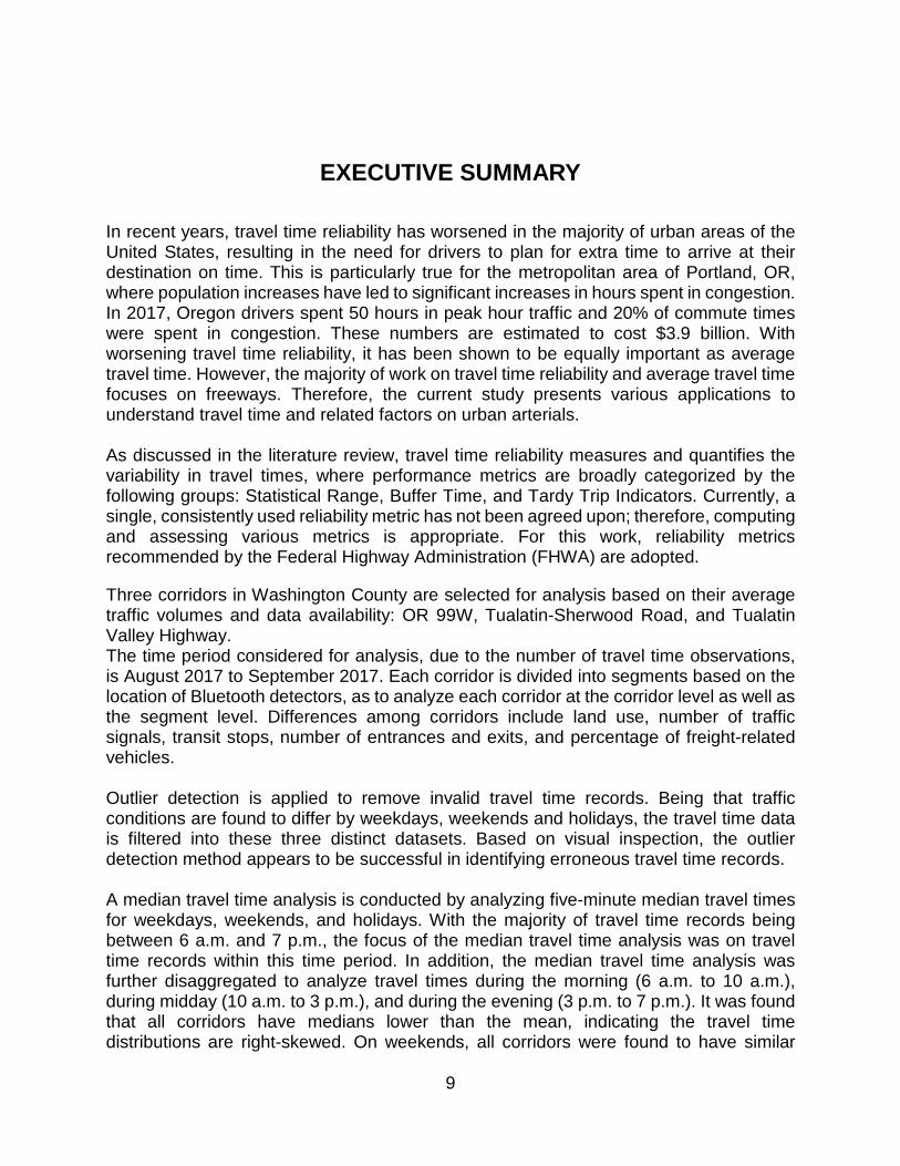
In recent years, travel time reliability has worsened in the majority of urban areas of the United States, resulting in the need for drivers to plan for extra time to arrive at their destination on time. This is particularly true for the metropolitan area of Portland, OR, where population increases have led to significant increases in hours spent in congestion. In 2017, Oregon drivers spent 50 hours in peak hour traffic and 20% of commute times were spent in congestion. These numbers are estimated to cost $3.9 billion. With worsening travel time reliability, it has been shown to be equally important as average travel time. However, the majority of work on travel time reliability and average travel time focuses on freeways. Therefore, the current study presents various applications to understand travel time and related factors on urban arterials. As discussed in the literature review, travel time reliability measures and quantifies the variability in travel times, where performance metrics are broadly categorized by the following groups: Statistical Range, Buffer Time, and Tardy Trip Indicators. Currently, a single, consistently used reliability metric has not been agreed upon; therefore, computing and assessing various metrics is appropriate. For this work, reliability metrics recommended by the Federal Highway Administration (FHWA) are adopted.

Three corridors in Washington County are selected for analysis based on their average traffic volumes and data availability: OR 99W, Tualatin-Sherwood Road, and Tualatin Valley Highway. The time period considered for analysis, due to the number of travel time observations, is August 2017 to September 2017. Each corridor is divided into segments based on the location of Bluetooth detectors, as to analyze each corridor at the corridor level as well as the segment level. Differences among corridors include land use, number of traffic signals, transit stops, number of entrances and exits, and percentage of freight-related vehicles. Outlier detection is applied to remove invalid travel time records. Being that traffic conditions are found to differ by weekdays, weekends and holidays, the travel time data is filtered into these three distinct datasets. Based on visual inspection, the outlier detection method appears to be successful in identifying erroneous travel time records. A median travel time analysis is conducted by analyzing five-minute median travel times for weekdays, weekends, and holidays. With the majority of travel time records being between 6 a.m. and 7 p.m., the focus of the median travel time analysis was on travel time records within this time period. In addition, the median travel time analysis was further disaggregated to analyze travel times during the morning (6 a.m. to 10 a.m.), during midday (10 a.m. to 3 p.m.), and during the evening (3 p.m. to 7 p.m.). It was found that all corridors have medians lower than the mean, indicating the travel time distributions are right-skewed. On weekends, all corridors were found to have similar

10

median travel time trends. However, on weekdays, peak median travel times varied by corridor and direction. As it pertains to statistics on travel time reliability metrics, the buffer index, planning index, and normalized standard deviation were presented. These metrics indicate that Tualatin-Sherwood Road has the lowest travel time reliability of the three corridors. It was also found that the westbound directions of Tualatin Valley Highway and Tualatin-Sherwood Road have slightly higher reliability compared to their eastbound directions. Of the selected corridors, OR 99W has the highest reliability, where the northbound is slightly more reliable than the southbound direction. In terms of time of day, mornings have the highest reliability and midday on weekends have the lowest reliability for all three corridors. At the segment level, shorter segments with a large number of entrances and exits have the lowest reliability. Through a bivariate modeling framework, significant factors on average travel time and travel time standard deviation were determined. In addition to determining such factors, their effects on average travel time and travel time standard deviation were quantified. Of the various methods to model travel time, the current work adopts a bivariate Tobit model to account for cross-equation correlation and the large number of zero observations for travel time standard deviation. Factors including morning peak hours, evening peak hours, weekend peak hours, and nighttime hours were found to be significant and have moderate to considerable effects on average travel time and travel time standard deviation. For nearly all factors, the largest effects (both positive and negative) on average travel time and travel time standard deviation are observed on Tualatin-Sherwood Road.

11

1.0 INTRODUCTION

The Moving Ahead for Progress in the 21st Century Act (MAP-21) established national performance goals for system reliability and seeks to improve the efficiency of the surface transportation system (Federal Highway Administration, 2012). Congestion is a critical problem in many urban areas in the United States. According to the 2015 Urban Mobility Scorecard, three billion gallons of fuel and seven billion extra hours were wasted due to congestion (Schrank et al., 2015b). Travel time reliability has worsened in most areas, and routinely, drivers have to plan for extra time than ever before in order to arrive just in time. According to the Federal Highway Administration’s Urban Congestion Report for October 2016, congestion trends as measured by metrics. such as number of congested hours and the travel and planning time index, all worsened in 2016 compared to 2015 (see Figure 1.1 below) (Federal Highway Administration, 2017a). Recent literature in modeling travel choices clearly shows that travel time reliability is as important as average travel time (Boyles et al., 2010; Pinjari and Bhat, 2006).

Figure 1.1: Congestion Trends in the United States (Source: Federal Highway Administration,

2017) Most of the existing reliability research has primarily focused on studying freeways in urban areas. There has been limited research on arterial corridors. While some research has focused on arterial travel time estimation and measurement (Liu et al., 2005; Kwong et al., 2009; Liu et al., 2006b), other researchers have studied arterial performance and ranking corridors for the purpose of traffic signal retiming (Day et al., 2015; Lavrenz et al., 2016).

12

1.1 RESEARCH OBJECTIVES

Past studies on travel time reliability have primarily focused on freeways. The primary objective of this study is to explore travel time reliability metrics on multimodal arterial corridors. The research seeks to answer the following key questions:

• What reliability-related metrics are currently being used or being considered for use in traffic planning and operations by practitioners and researchers for quantifying travel time reliability along arterial corridors?

• How can we best determine a viable method to detect and remove erroneous travel time records?

• Based on FHWA recommended travel time reliability metrics, how do multimodal arterials in Washington County, OR, perform?

• What factors impact average interval travel time and travel time standard deviation?

• What are the effects of identified factors on average interval travel time and travel time standard deviation?

13

2.0 LITERATURE REVIEW

2.1 INTRODUCTION

Travel time reliability and travel time variability are important metrics that can be used to describe the performance of the transportation system. According to the FHWA, travel time reliability is defined as the consistency or dependency in travel times as measured from day to day and/or across different times in a day (Federal Highway Administration, 2017b). According to Lomax et al. (2003), variability can be expressed as inconsistency in operating conditions. While both of these measures are important, reliability is more pertinent to travelers since it is related to their travel experience. Variability is related more to the facility and therefore more pertinent to transportation agencies (Lomax et al., 2003).

This chapter reviews the commonly used reliability measures and factors that impact travel time reliability and travel time distributions.

2.2 MEASURES

Performance measures that are used for reliability can be divided into three broad categories – Statistical Range, Buffer Time, and Tardy Trip Indicators. These are further described below. 2.2.1 Statistical Range Measures

These measures use standard deviation to represent the travel conditions that are experienced by travelers (Lomax et al., 2003). These are often represented as a deviation from the mean value. Measures that fall into this category include travel time window, percent variation, and variability index. • Travel Time Window

The average travel time is combined with the standard deviation to present a window within which travelers can expect their travel time to vary.

Travel Time Window = Average Travel Time ± Standard Deviation (2.1)

According to Lomax et al. (2003), this measure can be used for any mode or network size. • Percent Variation

Percent variation is the ratio between the standard deviation to the average travel time expressed as a percentage (Lomax et al., 2003). This measure is independent of trip

14

length, thus providing the ability to compare across different trip lengths. The ratio of standard deviation to average travel time is also known as the coefficient of variation.

Percent Variation =Standard Deviation

Average Travel Time× 100 (2.2)

• Variability Index

Variability index is a ratio of the peak to off-peak variation in travel conditions. This index is the ratio of the difference in the upper and lower 95% confidence intervals between the peak and off-peak period (Lomax et al., 2003):

Variability Index =(Upper 95% Value − Lower 95% Value)Peak

(Upper 95% Value − Lower 95% Value)Off−Peak (2.3)

Variability Index = Difference in peak – period confidence intervals (Upper 95% value – Lower 95% value) / Difference in Off –peak period confidence intervals (Upper 95% Value – Lower 95% Value). Additionally, percent variation or variability index can also be plotted graphically. • Standard Deviation

Standard deviation of travel times can also be used to characterize the variability in travel times (Day et al., 2015). Day et al. suggest that standard deviations should also be normalized with the speed limit travel times to account for varying lengths and speed limits.

𝑆𝑆′𝑇𝑇 = 𝑆𝑆𝑇𝑇𝑡𝑡𝑜𝑜

(2.4)

where 𝑆𝑆′𝑇𝑇 is the normalized standard deviation and 𝑆𝑆𝑇𝑇 is the raw standard deviation for time series 𝑇𝑇. Higher values of the normalized standard deviation imply greater unreliability. • Skew and Width

Van Lint and Van Zuylen (2005) propose measures based on the skew and width of the travel time distribution. The advantage of measures based on percentiles is that no assumption about the shape of the underlying travel distribution needs to be made. Skew is the ratio of the distance between the 90th and 50th percentile and the distance between the 50th and 10th percentile.

𝜏𝜏𝑠𝑠𝑠𝑠𝑠𝑠𝑠𝑠 = 𝑇𝑇90 − 𝑇𝑇50𝑇𝑇50 − 𝑇𝑇10

(2.5)

15

where 𝑇𝑇10 < 𝑇𝑇50 < 𝑇𝑇90. Van Lint and Van Zuylen (2005) suggest that the higher the skew, the higher the probability of extreme travel times that may occur relative to the median travel time. Width is the distance between the 90th and 50th percentile travel time relative to the median.

𝜏𝜏𝑣𝑣𝑣𝑣𝑣𝑣 = 𝑇𝑇90 − 𝑇𝑇10

𝑇𝑇50

(2.6)

Large values of 𝜏𝜏𝑣𝑣𝑣𝑣𝑣𝑣 indicate that the width of the travel time distribution is largely relative to its median value. • Combination of Skew and Width

Since 𝜏𝜏𝑠𝑠𝑠𝑠𝑠𝑠𝑠𝑠 and 𝜏𝜏𝑣𝑣𝑣𝑣𝑣𝑣 are very different for different freeway stretches, Van Lint and Zuylen (2005) propose a measure for travel time unreliability that removes the location specificity.

𝑈𝑈𝑈𝑈𝑣𝑣 = 𝜏𝜏𝑣𝑣𝑣𝑣𝑣𝑣 ln(𝜏𝜏𝑠𝑠𝑠𝑠𝑠𝑠𝑠𝑠)

𝐿𝐿𝑣𝑣 for 𝜏𝜏𝑠𝑠𝑠𝑠𝑠𝑠𝑠𝑠 > 1

𝑈𝑈𝑈𝑈𝑣𝑣 = 𝜏𝜏𝑣𝑣𝑣𝑣𝑣𝑣

𝐿𝐿𝑣𝑣 Otherwise

(2.7)

This measure indicates the likeliness of incurring a very bad travel time (Van Lint and Van Zuylen, 2005). The likeliness is large if either 𝜏𝜏𝑠𝑠𝑠𝑠𝑠𝑠𝑠𝑠 or 𝜏𝜏𝑣𝑣𝑣𝑣𝑣𝑣 or both are large. 2.2.2 Research Studies Using Statistical Range Measures

Day et al. (2015) studied travel times on arterial routes in Indiana using measures of central tendency (speed-normalized travel time) and variability (normalized standard deviation). They created a composite index that included the average value of travel time and its unreliability and used the index to rank arterials. Their findings revealed that routes with greater density of traffic signals tended to have higher average travel times and less reliability. Wang et al. (2017) used coefficient of variation of speed estimated from truck GPS data and developed a model using relationships between COV and density to forecast reliability. Ma et al. (2017b) used quantile regression to account for the heterogeneity in speed and coefficient of variation of speed to understand transit travel time reliability. Their findings revealed that the quantile regression model provided more indicative information compared to the mean-based regressions. Ma et al. used truck probe GPS data to forecast freeway travel time reliability using the coefficient of variation of spot speed

16

distribution. This study established relationships between travel time reliability and traffic density to forecast reliability for future traffic conditions. Bates et al. (2002) suggest that the median and percentile values provide more robust time-of-day and day-of-week estimates and easier means to reconstruct travel time distribution. Bates (2001) suggests using the 90th percentile to represent the upper bound of travel times.

2.3 BUFFER MEASURES

Buffer measures typically provide the extra time that travelers need to allot to their trip in order to arrive on time at their destination. This extra time or “buffer” reflects the uncertainty in travel conditions. Measures in this category include buffer time, buffer time index and planning time index. • Buffer Time

Buffer time is the extra time that is allotted to ensure on-time arrival. It is calculated as the difference between the average travel time and the 95th percentile travel time and expressed as:

Buffer Time (min) = 95th percentile travel time − Average travel time (2.8) • Buffer Index

Buffer index also represents the extra time that travelers need to allot for on-time arrival. It is computed as the difference between the 95th percentile travel time and the average travel time divided by the average travel time. It is expressed as a percentage. Higher values of the buffer index indicate greater unreliability.

Buffer Index = (95th percentile travel time − Average Travel Time)

Average Travel Time (2.9)

• Planning Time

Planning time refers to the total time that travelers allocate towards their trip. This measure includes buffer time. It is calculated as the 95th percentile travel time.

• Planning Time Index

Planning time index also refers to the total time that travelers allocate to their trip to ensure an on-time arrival. It differs from the buffer index because it also accounts for both typical and atypical delays (Federal Highway Administration, 2017b). It is computed as the 95th percentile travel time divided by the free-flow travel time.

17

Planning Time Index = 95th percentile travel timeFree − Flow Travel Time

(2.10)

• Travel Rate Envelope

Lomax et al. (2003) also suggest plotting the 5th and 95th percentile travel times for the peak period. The variation in conditions presented by these two travel times is similar to buffer time concepts. 2.3.1 Research Studies Using Buffer Measures

Lyman and Bertini (2008) studied the differences between buffer index, travel time index, and planning index for a segment on I-5 in Portland. The indices were estimated for one month of data over three consecutive years (the same month was used for estimation each year). Their findings revealed that while all three indices showed similar trends, the planning time index showed exaggerated trends when compared to the other two indices. Lyman and Bertini (2008) concluded that buffer index was the most conservative of all the indices studied. Pulugurtha and Imran (2017) used a microscopic simulation model to study density, travel time and density, and travel time reliability on freeways. Using planning time index measures, their findings revealed 95th percentile travel time decreased with a decrease in speed, but the 5th percentile travel time remained relatively constant. With buffer time index measures, they found that 95th and 50th percentile travel time values became closer as the speed limit decreased. They also examined the variation of planning time index (PTI) and buffer time index (BTI) as a function of speed limit and level of service (LOS). They found that the percent difference, when compared to the previous LOS-letter grade PTI threshold value, remains relatively similar with a slight increase or decrease in speed; however, for BTI threshold value the percent difference increases with a decrease in speed limit. Gong and Fan (2017) used travel time reliability measures such as frequency of congestion (FOC) and PTI to identify and rank recurrent freeway bottlenecks. FOC is defined as the percentage of travel times exceeding a threshold travel time or the percentage of travel speeds less than the threshold speed. Their results indicate that both FOC and PTI are capable of identifying and ranking bottlenecks. While previous research has found that the 95th percentile travel time is more susceptible to inclement weather or severe traffic crashes, this study found that 70% to 90% of the bottlenecks identified by the using the 80th percentile travel time are identical to those identified using the 95th percentile travel time. Their findings also indicate that using FOC or PTI alone may not be sufficient to quantify the intensity of traffic congestion caused by bottlenecks, and recommend that both travel time reliability and intensity measures be used together.

18

2.4 TARDY TRIP MEASURES

Tardy trip measures use the amount of late trips to measure system unreliability. Key measures in this category are the Florida Reliability Method, On-Time Arrival, and Misery Index.

• Florida Reliability Method

The Florida Reliability Method uses a proportion of average travel time in the peak period to estimate the limit of acceptable additional travel time range (Lomax et al., 2003), the Florida Reliability Statistic (FRS). Expected travel time is the sum of the average travel time and the additional travel time. The additional travel time can be defined by the user (e.g., 5%, 10%, 15%, 20% of the average). Travel times that are greater than the expected value are termed as unreliable trips. This statistic is calculated as follows:

FRS (% of Unreliable Trips)= 100% − (Percent trips with travel times greater than expected) (2.11)

• On-Time Arrival

Some studies have promoted the use of “lateness threshold” to determine unreliable trips (Lomax et al., 2003). An Urban Mobility Report produced by the Texas Transportation Institute suggested a threshold of 10% higher-than-average travel time (Schrank and Lomax, 1998). Lomax et al. (2003) state two concerns with this threshold. The acceptable late value may not vary linearly for each trip and is not related to trip duration. They also suggest that acceptable lateness may also be a function of the previous activity and the subsequent activity.

On − Time Arrival= 100%− (Percent of travel times greater than 110% of the average travel time)

(2.12)

• Misery Index

This measure estimates that average number of minutes the worst trips exceed the average (Lomax et al., 2003). It is estimated as follows:

Misery Index

= Average of travel rates for the longest 20% of trips − Average travel rates for all trips

Average travel rate

(2.13)

• Fosgerau’s Reliability Ratio

Fosgerau and Karlström (2010) proposed a reliability measure which is the ratio of the value of travel time variability to the value of time. They used Small’s delay model to

19

estimate the reliability ratio, in which the utility rate of arrival at the destination is a step function. 𝑤𝑤(𝑡𝑡) = 𝛼𝛼 − 𝛽𝛽, 𝑡𝑡 ≤ 𝑡𝑡∗ 𝑤𝑤(𝑡𝑡) = 𝛼𝛼 + 𝛾𝛾, 𝑡𝑡 > 𝑡𝑡∗ (2.14)

with the utility rate at the trip origin as a constant: ℎ(𝑡𝑡) = 𝛼𝛼 where 𝑡𝑡 is time of day, 𝑡𝑡∗ is the preferred arrival time and 𝛼𝛼, 𝛽𝛽 and 𝛾𝛾 are positive constants. The reliability ratio 𝜌𝜌 is estimated as:

𝜌𝜌 = 𝛽𝛽 + 𝛾𝛾𝛼𝛼

� 𝐹𝐹−1(𝑃𝑃) 𝑑𝑑𝑃𝑃1

𝛾𝛾𝛽𝛽+𝛾𝛾

(2.15)

where 𝐹𝐹−1(𝑃𝑃) is the inverse cumulative distribution function for the standardized travel time distribution and the integral is the mean lateness factor. The reliability ratio 𝜌𝜌 depends on traveler preference parameters 𝛼𝛼, 𝛽𝛽 and 𝛾𝛾 and the shape of the standardized travel time distribution, but does not depend on the mean travel time or the standard deviation.

2.5 PROBABILISTIC MEASURES

For these measures, travel time reliability is expressed as a probabilistic measure. Probabilistic travel measures often use a threshold travel time or a predefined window to differentiate between reliable and unreliable travel times (Van Lint et al., 2008). The Dutch Ministry of Transport, Public Works and Water Management proposed a reliability measure which stated that all trips should be made within 20% bounds of median travel time (Verker and Waterstaat, 2004).

2.6 FACTORS IMPACTING TRAVEL TIME RELIABILITY

Factors impacting travel time reliability are typically grouped into three categories: traffic influencing events, traffic demand, and physical features of the roadway (Kwon et al., 2011). These categories are further described below. 2.6.1 Traffic Influencing Events

This category includes factors that impact traffic such as traffic incidents, work zone activity and weather. • Traffic Incidents

20

This category is comprised of crashes and other incidents that can impact the traffic flow. Remedial actions include taking steps to prevent crashes and reacting promptly to incidents that occur in order to minimize the impacts (Kwon et al., 2011). • Work Zone Activity

This category is comprised of construction and other management activities. Measures that can be undertaken to reduce traffic impacts include better scheduling and execution of work zone activity. • Weather

Environmental conditions such as rain, fog, and snow comprise this category. Better response to adverse weather conditions can mitigate the impacts. 2.6.2 Traffic Demand

Factors in this category include fluctuations in daily demand and special events. • Fluctuations in Demand

The day-to-day fluctuations in demand also influence the reliability of travel times. Demand management strategies can help reduce the fluctuations in demand. • Special Events

Special events can have huge traffic impacts and, hence, can impact the reliability of travel times. Remedial measures include better planning of special events (Kwon et al., 2011). 2.6.3 Physical Features

This category includes traffic-control devices and inadequate base capacity. • Traffic-control Devices

Traffic-control devices such as railroad grade crossings and poorly timed traffic signals can also impact reliability. Optimizing the operation of signals and railroad grade crossings can help mitigate some of these impacts. • Inadequate Base Capacity

The roadway may contain physical bottlenecks that may constrain the demand. Remedial measures involve increasing the capacity (Kwon et al., 2011).

21

2.6.4 Research Studies

Kwon et al. (2011) studied the impact of the above-mentioned factors on buffer time, a measure of travel time reliability. They used 256 non-holiday weekdays of data from a freeway in the San Francisco Bay Area in California to estimate quantile regression models for three time periods: morning, noon, and afternoon. Their findings revealed that nonrecurrent factors (e.g., bottlenecks) impacted travel time reliability more during the afternoon than during the morning hours. The impact of traffic incidents was also highest during the afternoon, followed by morning and noon. The impact of weather was very small (2% to 5%) for all time periods. Work-zone contribution was highest at noon (13%), followed by afternoon (9%) and morning (5%). Special-event impacts were largely seen at noon (11.4%) and afternoon (0.9%) periods, but the coefficients were not statistically significant. A guide developed by the Strategic Highway Research Program (SHRP2) provides guidance on establishing monitoring programs for travel time reliability, including measuring, characterizing, identifying, and understanding the effects of recurrent and nonrecurrent events that affect travel time reliability (List et al., 2014).

2.7 TRAVEL TIME DISTRIBUTION

In order to fully understand travel time reliability on arterials, the shape of the travel time distribution (TTD) also needs to be studied. However, compared to freeways, travel time distribution estimation on arterials is more complex. Chen et al. (2014) found that TTD on arterials varies based on different levels of congestion, possibly due to varying traffic regimes, signal control strategies and correlation between neighboring segments. On arterials, most of the research has been focused on travel time estimation (Highway Capacity Manual, 2010; Skabardonis and Geroliminis, 2005, 2008; Liu and Ma, 2009). There is limited research on the segment-level and path-level variability in TTD. Ji and Zhang (2013) used high-resolution bus probe data for segment travel time estimation and found a bimodal distribution, with one mode corresponding to travel times without delay and the other mode corresponding to travel times with delay. Zheng and Van Zuylen (2011) studied the delay distributions at signalized intersections in order to understand segment-level TTD using stochastic arrivals and departures at signals. Their findings revealed a temporal correlation between arrival time and segment travel time. Path-level TTD is more important to travelers than segment-level TTD (Chen et al., 2017). Many studies have used unimodal distributions such as Normal, Lognormal, Gamma, Weibull, Exponential and Burr to characterize TTD on a path (Emam and Al-Deek, 2006; Uno et al., 2009; Susilawati et al., 2013; Taylor, 2017). Recently, however, researchers have found that the unimodal distribution may not accurately represent TTD because travel times during free-flow and congested conditions differ greatly (Guo et al., 2010; Feng et al., 2012; Kazagli and Koutsopoulos, 2013; Chen et al., 2014). TTD have strong skew and heavy upper-tail weight. Guo et al. (2010) used a mixture of Gaussian distributions to model travel times along an arterial in San Antonio. Feng et al. (2012) used GPS probe vehicles to estimate TTD using a mixture of normal distributions. Kazagli and Koutsopoulos (2013) used AVI data and a mixture of two

22

lognormal distributions to model travel times on arterials. Chen et al. (2014) used a regression model with varying weights to study path TTD in an urban area considering signal timings. Most segment-level or path-level TTD estimation procedures assume independence of segment travel times. Chen et al. (2017) suggest that this assumption may be warranted when estimating average travel times but not for estimating TTD. He et al. (2002) suggest that the assumptions made of long-term TTD estimation, such as peak hours, non-peak hours, seasonal and daily, may not be valid for short-term TTD estimation. Using Paramics simulation environment, He et al. studied the temporal and spatial variations in travel times and found a significant correlation between segment travel times. They suggest that the path TTD needs to account for correlation between individual segments and that route guidance should incorporate both temporal and spatial variability in travel times. Pattanamekar et al. (2003) used a joint probability distribution function to estimate the conditional mean and variance on one segment given the observations on the other segments. Rakha et al. (2006) suggested that the assumption of segment travel-time independence does not account for covariance. Using the segment-level dependencies between travel time variances, they estimated the freeway path travel time. Geroliminis and Skabardonis (2006) assumed linear correlation between successive segment travel times to estimate the variance of one urban route travel time. Herring et al. (2010) used a coupled Hidden Markov chain model to estimate TTD for segments using probe-vehicle data. Herring et al. found that TTD is correlated to the states of the spatial neighbors of the segment but independent from all the other variables. Ramezani and Geroliminis (2015) predicted path TTD using Markov chains, assuming that transition between different segment pairs are conditionally independent. Westgate et al. (2016) estimated a regression model to estimate TTD for ambulance travel times at the trip level, assuming dependence in segment travel times. Chen et al. (2017) used a copula-based approach to characterize the dependence between segment travel times. Their findings revealed that multimodal distributions are better for characterizing segment-level TTDs and dependencies between segment travel times were weak at the spatial aggregation used.

2.8 SUMMARY

This chapter reviewed the published literature on travel time reliability measures, factors affecting travel time reliability, and methods to estimate travel time distributions. Travel time reliability measures quantify the variability in travel times. Performance measures that are used for reliability are divided into three broad categories – Statistical Range, Buffer Time, and Tardy Trip Indicators. Research has not agreed upon one single measure, and it may be appropriate to compute several reliability measures depending upon availability of resources. The current version of the urban mobility report uses planning time index, travel time index and commuter stress index (measure of extra travel time for a commuter) to quantify freeway reliability (Schrank et al., 2015a). Factors affecting travel time reliability include incidents, work zones, weather, fluctuations in demand, special events, traffic control devices, and inadequate base capacity. A good

23

monitoring system should capture the contribution of each of these factors towards total variability (Lomax et al., 2003). Research on arterial travel time distributions is still evolving. Recent studies have found that unimodal distributions may not accurately represent TTDs and the assumption of independence of segment travel times does not hold.

24

3.0 DESCRIPTIVE STATISTICS

Three corridors in Washington County were selected for the analysis. We first describe the selection procedure and provide a comparison of roadway, geometric, and land use data along the corridors. An outlier detection method is outlined. We then provide a detailed descriptive statistical analysis of selected travel time reliability metrics for the three corridors .

3.1 CORRIDOR SELECTION

For this study, six corridors in Washington County were originally considered for the analysis:

• Cornell Road • Cornelius Pass Road • OR 99W • Murray Blvd • Tualatin-Sherwood Road • Tualatin Valley Highway

Based on the data availability and average traffic volumes, the following three corridors in both directions were selected for the travel time reliability analysis:

• OR 99W • Tualatin-Sherwood Road • Tualatin Valley Highway

Figure 3.1 to Figure 3.3 show the selected corridors. In these figures, the segments within each corridor, each segment’s beginning and ending location, and the length of each segment are defined. The analysis of the three corridors considers four months of data, August 2017 to November 2017. Since the majority of trips occur between 6 a.m. and 7 p.m., only observations within this period were considered. The travel time data for the selected corridors was collected from the website of BlueMAC1 Transportation Data Systems. In 2016, about 120 Bluetooth detector devices, called BlueMAC devices, were installed in Washington County to improve the commuter experience . Each BlueMAC deice is located at an intersection on various arterials . The vehicle capture rate of these BlueMAC devices is higher than 10% of the traffic for target corridors . From this website, one can select any two specific BlueMAC devices, one as the start and the other as the end point of the desired section of road, to get all of the travel times recorded by these detectors.

1 BlueMAC Analytics. Accessed at http://washcobm.digiwest.com/

25

Figure 3.2: Tualatin-Sherwood Road (OR 99W to I-5 SB On-Ramp)

Figure 3.1: Tualatin Valley Highway (SE Brookwood Ave to SW Lombard Ave)

26

Figure 3.3: OR 99W (SW Tualatin-Sherwood Rd. to SW Durham Rd.) Each of these selected corridors has different characteristics. For example, compared to Tualatin Valley Highway and Tualatin-Sherwood Road, OR 99W has very few traffic signals. Furthermore, Tualatin Valley Highway has a higher number of transit stops and has frequent bus service along the corridor. On the other hand, OR 99W and Tualatin-Sherwood Road only have a single major transit stop and the bus service frequency is less. These are examples of characteristics that can impact travel time. Table 3.1 provides a summary of the characteristics that can potentially influence travel times along the selected corridors.

27

Table 3.1: Summary of Selected Corridors Corridor Tualatin Valley

Highway Tualatin-Sherwood Road OR 99W

Start Location SE Tualatin Valley Highway and SE Brookwood Ave

SW Tualatin-Sherwood Road and OR 99W

OR 99W and SW Tualatin-Sherwood Road

End Location SW Canyon Road and SW Lombard Ave

SW Nyberg Street and I-5

OR 99W and SW Durham Road

Length (Miles) 6.42 4.66 3.56 Select Average Traffic Volumes

• 0.21% Motorcycles • 12.44% Four Tire,

Single Unit • 0.83% Buses • 1.32% Two Axle, Six

Tire, Single Unit • 0.56% 5-Axle Tractor

Semi Trailer • 0.15% Six or More

Axle Single Trailer





Axle Single Trailer





Axle, Single Trailer Land Use

• Industrial • General Commercial • Community Business

District • Neighborhood

Commercial • Residential District

(25 Units or More Per Acre)

• Institutional

• Industrial

• Industrial • Exclusive Farm Use • Agriculture and

Forest (20 Acre Minimum)

• Agriculture and Forest (5 Acre Minimum)

• Land Extensive Industrial

• Rural Residential (5 Acre Minimum)

• Residential District (24 Units Per Acre)

Traffic Signals 18 18 8 The three corridors considered for analysis are divided into multiple segments based on their geometric design. Table 3.2 to Table 3.7 summarize the characteristics of the individual segments by direction within each corridor. Table 3.2 and Table 3.3 provide the characteristics of each segment along the eastbound and westbound directions of Tualatin Valley Highway, respectively. In the eastbound direction, segments 4 and 5 are the smallest segments. Segment 5 in the eastbound direction and segment 1 in the westbound direction, which corresponds to the section between Lombard Avenue and Cedar Hills Boulevard, has a high number of entrances and exits per mile, which could cause substantial interruptions for the traffic flow. The westbound direction has a higher (nearly triple) number of entrances and exits relative to the eastbound direction.

28

Table 3.2: Segment-level Summary of Tualatin Valley Highway (Eastbound)

Segment Start Location End Location Length (Miles) Lanes Traffic

Signals Transit Stops

Entrances and Exits

01 Tualatin Valley Hwy and Brookwood Ave

Tualatin Valley Hwy and Cornelius Pass Rd.

1.46 2 3 4 1

02


Tualatin Valley Hwy and 185th Ave

1.71 2 4 7 10

03 Tualatin Valley Hwy and 185th Ave

Tualatin Valley Hwy and Murray Blvd.

2.03 2 to 3 5 8 2

04 Tualatin Valley Hwy and Murray Blvd.

Tualatin Valley Hwy and Cedar Hills Blvd.

0.75 3 to 2 2 2 3

05 Tualatin Valley Hwy and Cedar Hills Blvd.

Canyon Rd. and Lombard Ave 0.47 2 3 2 10

Table 3.3: Segment-level Summary of Tualatin Valley Highway (Westbound) Segment Start Location End Location Length

(Miles) Lanes Traffic Signals

Transit Stops

Entrances and Exits

01 Canyon Rd. and Lombard Ave

Tualatin Valley Hwy and Cedar Hills Blvd.

0.47 2 2 3 18


Tualatin Valley Hwy and Murray Blvd.

0.75 2 4 2 14


Tualatin Valley Hwy and 185th Ave

2.03 3 to 2 5 8 22



1.71 2 to 3 2 7 35

05


Tualatin Valley Hwy and Brookwood Ave

1.46 2 4 4 16

29

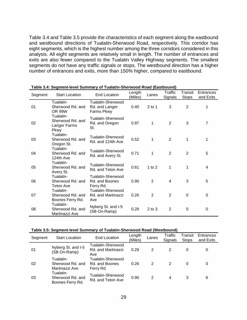
Table 3.4 and Table 3.5 provide the characteristics of each segment along the eastbound and westbound directions of Tualatin-Sherwood Road, respectively. This corridor has eight segments, which is the highest number among the three corridors considered in this analysis. All eight segments are relatively small in length. The number of entrances and exits are also fewer compared to the Tualatin Valley Highway segments. The smallest segments do not have any traffic signals or stops. The westbound direction has a higher number of entrances and exits, more than 150% higher, compared to eastbound. Table 3.4: Segment-level Summary of Tualatin-Sherwood Road (Eastbound)



Entrances and Exits

01 Tualatin-Sherwood Rd. and OR 99W

Tualatin-Sherwood Rd. and Langer Farms Pkwy

0.40 2 to 1 3 2 1

02


Tualatin-Sherwood Rd. and Oregon St.

0.97 1 2 3 7

03 Tualatin-Sherwood Rd. and Oregon St.

Tualatin-Sherwood Rd. and 124th Ave 0.52 1 2 1 1

04 Tualatin-Sherwood Rd. and 124th Ave

Tualatin-Sherwood Rd. and Avery St. 0.71 1 2 2 5

05 Tualatin-Sherwood Rd. and Avery St.

Tualatin-Sherwood Rd. and Teton Ave 0.61 1 to 2 1 1 4

06 Tualatin-Sherwood Rd. and Teton Ave

Tualatin-Sherwood Rd. and Boones Ferry Rd.

0.90 2 4 3 5

07 Tualatin-Sherwood Rd. and Boones Ferry Rd.

Tualatin-Sherwood Rd. and Martinazzi Ave

0.26 2 2 0 0

08 Tualatin-Sherwood Rd. and Martinazzi Ave

Nyberg St. and I-5 (SB On-Ramp) 0.29 2 to 3 2 0 0

Table 3.5: Segment-level Summary of Tualatin-Sherwood Road (Westbound)



Entrances and Exits

01 Nyberg St. and I-5 (SB On-Ramp)


0.29 2 2 0 0



0.26 2 2 0 0


Tualatin-Sherwood Rd. and Teton Ave 0.90 2 4 3 6

30



Entrances and Exits


Tualatin-Sherwood Rd. and Avery St. 0.61 2 to 1 1 1 1


Tualatin-Sherwood Rd. and 124th Ave 0.71 1 2 1


Tualatin-Sherwood Rd. and Oregon St.

0.52 1 2 2 3



0.97 1 3 2 7

08


Tualatin-Sherwood Rd. and OR 99W 0.40 1 to 2 2 1 2

Table 3.6 and Table 3.7 give the characteristics of each segment along the northbound and southbound directions of OR 99W, respectively. This corridor only has two segments, which is the smallest number among the three corridors in this analysis. Considering all the traffic obstructions per mile, including signals, transit stops, entrances and exits, segment 2 might be facing the highest interruptions to traffic flow. The southbound direction has a 50% higher number of entrances and exits per mile relative to the northbound direction. However, the northbound direction has nearly 50% higher number of transit stops per mile. Table 3.6: Segment-level Summary of OR 99W (Northbound)



Entrances and Exits

01 OR 99W & Tualatin-Sherwood Rd.

OR 99W & 124th Ave 2.35 3 to 2 3 3 15

02 OR 99W & 124th Ave

OR 99W & Durham Rd. 1.21 2 4 5 10

Table 3.7: Segment-level Summary of OR 99W (Southbound)



Entrances and Exits

01 OR 99W & Durham Rd.

OR 99W & 124th Ave 1.21 2 4 2 17

02 OR 99W & 124th Ave

OR 99W & Tualatin-Sherwood Rd.

2.35 2 to 3 3 5 19

31

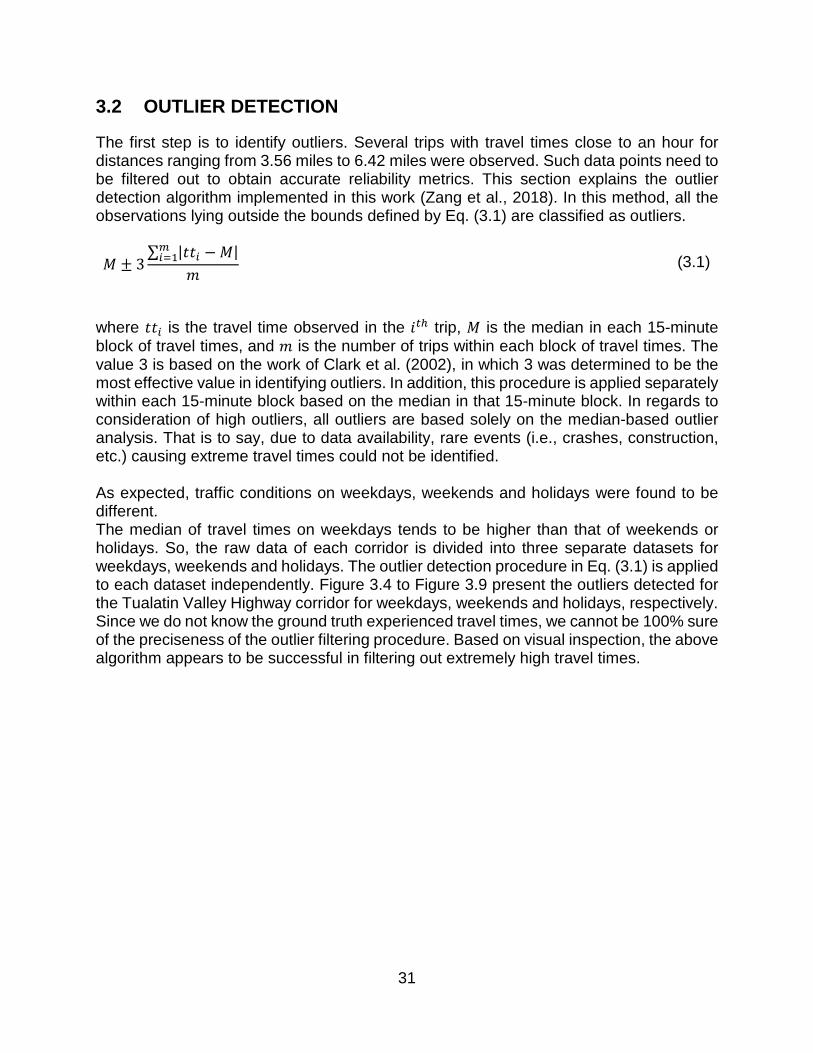
3.2 OUTLIER DETECTION

The first step is to identify outliers. Several trips with travel times close to an hour for distances ranging from 3.56 miles to 6.42 miles were observed. Such data points need to be filtered out to obtain accurate reliability metrics. This section explains the outlier detection algorithm implemented in this work (Zang et al., 2018). In this method, all the observations lying outside the bounds defined by Eq. (3.1) are classified as outliers.

𝑀𝑀 ± 3∑ |𝑡𝑡𝑡𝑡𝑖𝑖 − 𝑀𝑀|𝑚𝑚𝑖𝑖=1

𝑚𝑚 (3.1)

where 𝑡𝑡𝑡𝑡𝑖𝑖 is the travel time observed in the 𝑖𝑖𝑡𝑡ℎ trip, 𝑀𝑀 is the median in each 15-minute block of travel times, and 𝑚𝑚 is the number of trips within each block of travel times. The value 3 is based on the work of Clark et al. (2002), in which 3 was determined to be the most effective value in identifying outliers. In addition, this procedure is applied separately within each 15-minute block based on the median in that 15-minute block. In regards to consideration of high outliers, all outliers are based solely on the median-based outlier analysis. That is to say, due to data availability, rare events (i.e., crashes, construction, etc.) causing extreme travel times could not be identified. As expected, traffic conditions on weekdays, weekends and holidays were found to be different. The median of travel times on weekdays tends to be higher than that of weekends or holidays. So, the raw data of each corridor is divided into three separate datasets for weekdays, weekends and holidays. The outlier detection procedure in Eq. (3.1) is applied to each dataset independently. Figure 3.4 to Figure 3.9 present the outliers detected for the Tualatin Valley Highway corridor for weekdays, weekends and holidays, respectively. Since we do not know the ground truth experienced travel times, we cannot be 100% sure of the preciseness of the outlier filtering procedure. Based on visual inspection, the above algorithm appears to be successful in filtering out extremely high travel times.

32

Figure 3.4: Outliers in Travel Times on Tualatin Valley Hwy (Eastbound) on Weekdays

Figure 3.5: Outliers in Travel Times on Tualatin Valley Hwy (Eastbound) on Weekends Figure 3.6: Outliers in Travel Times on Tualatin Valley Hwy (Eastbound) on Holidays Figure 3.7: Outliers in Travel Times on Tualatin Valley Hwy (Westbound) on Weekdays

33

Figure 3.8: Outliers in Travel Times on Tualatin Valley Hwy (Westbound) on Weekends

Figure 3.9: Outliers in Travel Times on Tualatin Valley Hwy (Westbound) on Holidays

34

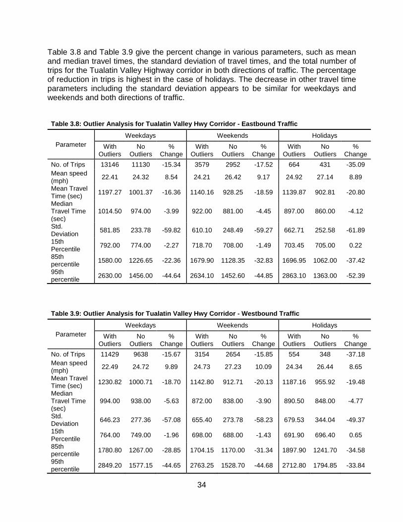
Table 3.8 and Table 3.9 give the percent change in various parameters, such as mean and median travel times, the standard deviation of travel times, and the total number of trips for the Tualatin Valley Highway corridor in both directions of traffic. The percentage of reduction in trips is highest in the case of holidays. The decrease in other travel time parameters including the standard deviation appears to be similar for weekdays and weekends and both directions of traffic. Table 3.8: Outlier Analysis for Tualatin Valley Hwy Corridor - Eastbound Traffic

Parameter Weekdays Weekends Holidays

With Outliers

No Outliers

% Change

With Outliers

No Outliers

% Change

With Outliers

No Outliers

% Change

No. of Trips 13146 11130 -15.34 3579 2952 -17.52 664 431 -35.09 Mean speed (mph) 22.41 24.32 8.54 24.21 26.42 9.17 24.92 27.14 8.89

Mean Travel Time (sec) 1197.27 1001.37 -16.36 1140.16 928.25 -18.59 1139.87 902.81 -20.80

Median Travel Time (sec)

1014.50 974.00 -3.99 922.00 881.00 -4.45 897.00 860.00 -4.12

Std. Deviation 581.85 233.78 -59.82 610.10 248.49 -59.27 662.71 252.58 -61.89

15th Percentile 792.00 774.00 -2.27 718.70 708.00 -1.49 703.45 705.00 0.22

85th percentile 1580.00 1226.65 -22.36 1679.90 1128.35 -32.83 1696.95 1062.00 -37.42

95th percentile 2630.00 1456.00 -44.64 2634.10 1452.60 -44.85 2863.10 1363.00 -52.39

Table 3.9: Outlier Analysis for Tualatin Valley Hwy Corridor - Westbound Traffic


With Outliers

No Outliers

% Change

With Outliers

No Outliers

% Change

With Outliers

No Outliers

% Change




994.00 938.00 -5.63 872.00 838.00 -3.90 890.50 848.00 -4.77

Std. Deviation 646.23 277.36 -57.08 655.40 273.78 -58.23 679.53 344.04 -49.37

15th Percentile 764.00 749.00 -1.96 698.00 688.00 -1.43 691.90 696.40 0.65

85th percentile 1780.80 1267.00 -28.85 1704.15 1170.00 -31.34 1897.90 1241.70 -34.58

95th percentile 2849.20 1577.15 -44.65 2763.25 1528.70 -44.68 2712.80 1794.85 -33.84

35

Table 3.10 and Table 3.11 give the percentage changes in various parameters for the Tualatin-Sherwood Road corridor in both directions of traffic. The percentage of change in each parameter is almost the same for weekdays and weekends irrespective of the direction of traffic. Table 3.10: Outlier Analysis for Tualatin-Sherwood Road Corridor - Eastbound Traffic


With Outliers

No Outliers

% Change

With Outliers

No Outliers

% Change

With Outliers

No Outliers

% Change




822.50 756.00 -8.09 637.00 606.00 -4.87 613.00 588.00 -4.08

Std. Deviation 722.67 328.41 -54.56 646.11 212.48 -67.11 646.68 236.04 -63.50

15th Percentile 525.00 506.00 -3.62 480.00 469.00 -2.29 475.30 474.00 -0.27

85th percentile 1773.95 1139.00 -35.79 1266.40 810.00 -36.04 1279.70 828.00 -35.30

95th percentile 2853.65 1499.00 -47.47 2546.20 1085.00 -57.39 2508.15 1142.50 -54.45

Table 3.11: Outlier Analysis for Tualatin-Sherwood Road Corridor - Westbound Traffic


With Outliers

No Outliers

% Change

With Outliers

No Outliers

% Change

With Outliers

No Outliers

% Change




775.00 720.00 -7.10 607.00 582.00 -4.12 601.00 567.50 -5.57

Std. Deviation 740.39 330.06 -55.42 656.99 213.36 -67.52 722.85 293.10 -59.45

15th Percentile 529.00 510.00 -3.59 477.00 467.00 -2.10 464.00 458.00 -1.29

85th percentile 1826.00 1114.00 -38.99 1252.00 774.00 -38.18 1540.00 804.25 -47.78

95th percentile 2894.00 1530.00 -47.13 2560.35 1093.00 -57.31 2784.30 1350.00 -51.51

36

Table 3.12 and Table 3.13 give the percentage changes in various parameters for the OR 99W corridor in both directions of traffic. Among the three corridors, OR 99W has the least percent of the reduction in the total number of trips and median of travel times. However, OR 99W has the highest percentage of the reduction in standard deviation. Table 3.12: Outlier Analysis for OR 99W Corridor - Northbound Traffic


With Outliers

No Outliers

% Change

With Outliers

No Outliers

% Change

With Outliers

No Outliers

% Change



Median Travel Time (sec) 358.00 350.00 -2.23 324.00 317.00 -2.16 321.00 317.00 -1.25

Std. Deviation 487.12 86.34 -82.28 480.01 72.23 -84.95 482.44 93.49 -80.62 15th Percentile 288.00 285.00 -1.04 271.00 269.00 -0.74 266.00 266.00 0.00

85th percentile 490.00 436.00 -11.02 418.00 382.00 -8.61 420.00 388.00 -7.62

95th percentile 1497.00 519.00 -65.33 1446.00 434.00 -69.99 1302.10 451.00 -65.36

Table 3.13: Outlier Analysis for OR 99W Corridor - Southbound Traffic


With Outliers

No Outliers

% Change

With Outliers

No Outliers

% Change

With Outliers

No Outliers

% Change



Median Travel Time (sec) 353.00 344.00 -2.55 327.00 321.00 -1.83 326.00 318.00 -2.45

Std. Deviation 543.78 116.57 -78.56 567.09 90.80 -83.99 520.38 111.55 -78.56 15th Percentile 283.00 281.00 -0.71 276.00 274.00 -0.72 271.00 269.00 -0.74

85th percentile 600.00 480.00 -20.00 445.00 385.00 -13.48 511.60 399.00 -22.01

95th percentile 1793.00 625.00 -65.14 1887.65 468.00 -75.21 1539.70 547.30 -64.45

37

For all three corridors, the percentage reduction in trips appears to be consistent across both directions and for weekdays and weekends. The holidays in some cases have different percentage changes. This could be potentially due to sample size issues or because holidays have different travel time patterns. All the corridors have medians lower than the mean, indicating the presence of right skew in the travel time distribution. After removing outliers, Tualatin-Sherwood and OR 99W have higher standard deviations on weekdays compared to weekends, showing lower reliability on weekdays which is expected. For the Tualatin Valley Highway corridor, the standard deviation was almost the same for weekdays and weekends in the westbound direction, and the standard deviation was slightly higher for weekends in the eastbound direction.

3.3 MEDIAN TRAVEL TIME ANALYSIS

In this section, we analyze the five-minute median travel times for weekdays, weekends and holidays separately and identify trends in peak hours. After removing the outliers, the median travel times for five-minute intervals were determined for each corridor in each direction. For the intervals with no data, the travel times were set to zero for graphical identification and to avoid errors during calculations. Tukey's Smoothing tool (R Core Team, 2019) was applied to the median curves of all the corridors to distinguish the peaks clearly. Within each day, the following time-periods are defined:

• Morning: 6 a.m. to 10 a.m. • Midday: 10 a.m. to 3 p.m. • Evening: 3 p.m. to 7 p.m.

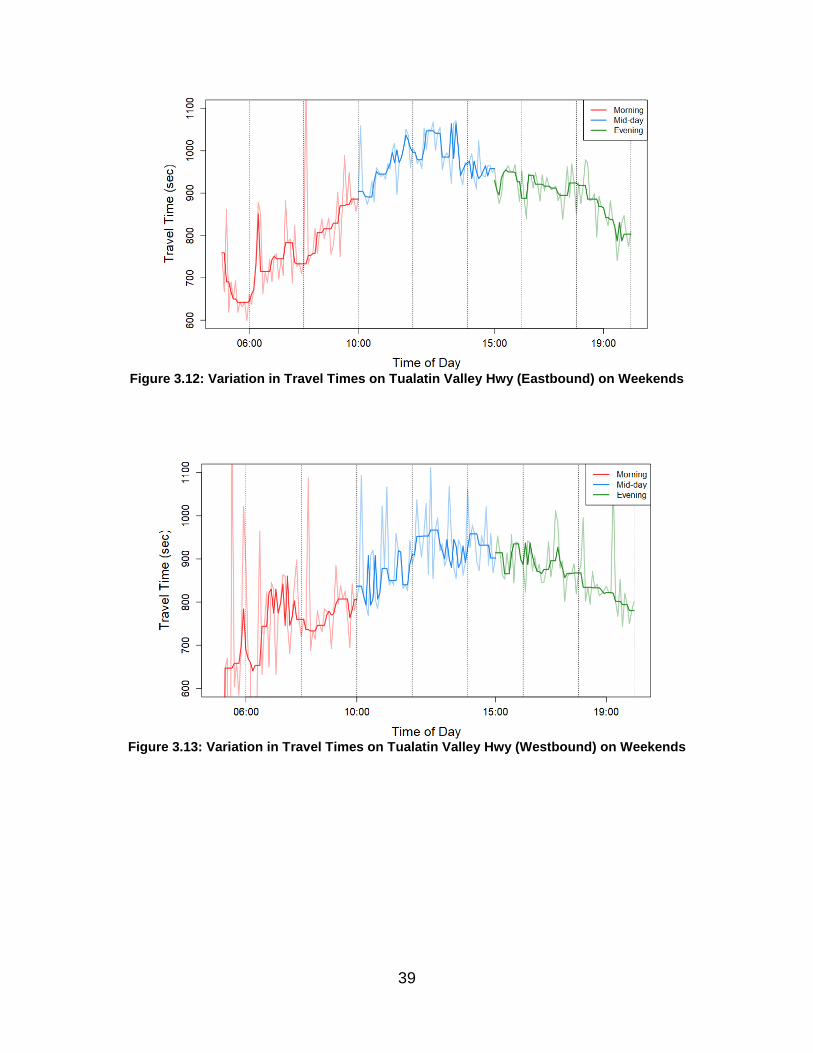
Figure 3.10 to Figure 3.15 show the variations in five-minute median travel times over Tualatin Valley Highway in the eastbound and westbound direction on weekdays, weekends and holidays. During the weekdays, there are two peaks, a sharper morning peak and a broader evening peak. In the eastbound direction, the travel time during the morning peak (around 7 a.m.) is higher whereas, in the westbound direction, the evening peak (between 5 p.m. and 6 p.m.) is more pronounced. In the westbound direction, during weekdays the travel times during midday becomes higher than the morning peak. Whereas, on weekends and holidays, the travel times gradually increase and decrease with the highest travel times observed between 12 p.m. and 2 p.m. in both directions. Also, in the case of holidays, the dataset is small and it doesn't have records for all intervals.

38

Figure 3.10: Variation in Travel Times on Tualatin Valley Hwy (Eastbound) on Weekdays

Figure 3.11: Variation in Travel Times on Tualatin Valley Hwy (Westbound) on Weekdays

39

Figure 3.12: Variation in Travel Times on Tualatin Valley Hwy (Eastbound) on Weekends

Figure 3.13: Variation in Travel Times on Tualatin Valley Hwy (Westbound) on Weekends

40

Figure 3.14: Variation in Travel Times on Tualatin Valley Hwy (Eastbound) on Holidays

Figure 3.15: Variation in Travel Times on Tualatin Valley Hwy (Westbound) on Holidays

Figure 3.16 to Figure 3.21 show the five-minute median travel time variations of Tualatin-Sherwood Road. During the weekday in the eastbound direction, the travel times show a sharp morning peak and a broader peak covering midday and evening, with the highest travel times between 2 p.m. and 3 p.m. In the weekdays in the westbound direction, there are three distinct peaks – morning, midday and evening of increasing magnitude. On weekends, the travel times gradually increase and decrease, with the highest travel times observed between 12 p.m. and 2 p.m. in both directions. No trends are observed during the holidays.

41

Figure 3.16: Variation in Travel Times on Tualatin-Sherwood Road (Eastbound) on Weekdays

Figure 3.17: Variation in Travel Times on Tualatin-Sherwood Road (Westbound) on Weekdays

42

Figure 3.18: Variation in Travel Times on Tualatin-Sherwood Road (Eastbound) on Weekends

Figure 3.19: Variation in Travel Times on Tualatin-Sherwood Road (Westbound) on Weekends

43

Figure 3.20: Variation in Travel Times on Tualatin-Sherwood Road (Eastbound) on Holidays

Figure 3.21: Variation in Travel Times on Tualatin-Sherwood Road (Westbound) on Holidays

Figure 3.22 to Figure 3.27 depict the variations of travel times along OR 99W. In both the northbound and southbound directions on weekdays, the evening peak dominates. On weekdays, there is a smaller morning peak in the northbound direction, whereas no morning peak is observed in the southbound direction. The fluctuations are lower on OR 99W compared to the previous two corridors. On weekends, the travel times gradually increase and decrease, with the highest travel times observed between noon and 2 p.m. in both directions.

44

Figure 3.22: Variation in Travel Times on OR 99W (Northbound) on Weekdays

Figure 3.23: Variation in Travel Times on OR 99W (Southbound) on Weekdays

45

Figure 3.24: Variation in Travel Times on OR 99W (Northbound) on Weekends

Figure 3.25: Variation in Travel Times on OR 99W (Southbound) on Weekends

46

Figure 3.26: Variation in Travel Times on OR 99W (Northbound) on Holidays

Figure 3.27: Variation in Travel Times on OR 99W (Southbound) on Holidays

To summarize, all three corridors exhibit similar travel time trends on weekends. However, the weekday peak travel time trends vary depending on direction and corridor.

47

3.4 DESCRIPTIVE STATISTICS OF RELIABILITY METRICS

This section first provides a detailed descriptive statistical analysis of the reliability of the selected corridors. We then compare the reliability of segments within each corridor. The reliability metrics used in this analysis are:

i. Buffer Index: The difference between the 95th percentile of travel times and the mean of travel times is called the buffer time, which refers to the extra time needed by the travelers to ensure on-time arrival. The ratio of the buffer time to the mean travel time is called the buffer index.

Buffer Index = (95th Percentile Travel Time − Mean Travel Time)

Mean Travel Time

(3.2)

ii. Normalized Standard Deviation: The normalized standard deviation is defined

as the ratio of the standard deviation of the travel times to the free-flow travel time.

Normalized SD = Standard Deviation of Travel Time

Free − Flow Travel Time

(3.3)

iii. Planning Index: The 95th percentile of travel times is called the planning time,

which refers to the total time that needs to be allocated to the trip to ensure on-time arrival at least for 95% of the trips. The ratio of this planning time to the free-flow travel time is called the planning index.

Planning Index = 95th Percentile Travel Time

Free − Flow Travel Time

(3.4)

Buffer and planning indexes are reliability metrics recommended by the FHWA ( 2017b). We also picked normalized standard deviation as standard deviation is a common metric used for comparing variability. 3.4.1 Corridor Level Analysis

The free-flow travel times of each corridor was estimated by adding the free-flow travel times of all the segments in that corridor. The free-flow speed of each segment in that corridor was assumed to be 5 miles per hour more than the speed limit of that segment (Moses and Mtoi, 2013). Then the free-flow travel time of each segment was found by dividing their respective lengths with the free-flow speeds. The free-flow travel time of each corridor is estimated by summing the free-flow travel times of all the segments. Table 3.14 gives the free-flow travel times and speeds of all the corridors. As expected,

48

there are no differences in free-flow travel times or speeds by direction. The Tualatin Valley Highway has the highest free-flow travel times, whereas OR 99W has the lowest free-flow travel times. This is consistent with the length of the corridors.

Table 3.14: Free-flow Travel Times and Speeds of all Corridors

Corridor Direction Free-flow Travel Time (sec)

Free-flow Speed (mph)

Tualatin Valley Highway Eastbound 506 46 Westbound 502 46

Tualatin-Sherwood Road

Eastbound 357 47 Westbound 358 47

OR 99W Northbound 236 55 Southbound 238 55

Table 3.15 provides the mean, median, and reliability metrics for each corridor. Each statistic was calculated for 15-minute time intervals from 6 a.m. to 7 p.m. and then averaged to get the overall statistic for each corridor. Note that the higher the value of the reliability metrics, the lower the travel time reliability. The Tualatin Valley Highway, which is the longest corridor, has the highest mean and median travel time. Tualatin-Sherwood Road has the lowest reliability. For both Tualatin Valley and Tualatin-Sherwood, the eastbound direction has marginally higher median travel times as well as slightly higher reliability compared to the westbound direction. OR 99W corridor has the lowest mean and median travel time and the highest reliability among the selected corridors. The northbound direction of OR 99W has marginally higher reliability than the southbound direction. Table 3.15: Overall Descriptive Statistics of all Corridors

Corridor Direction Mean Travel Time

Median Travel Time

Standard Deviation

Buffer Index

Normalized SD

Planning Index

Tualatin Valley Highway

Eastbound 987 955 171 0.31 0.34 2.59 Westboun

d 964 901 223 0.41 0.44 2.76


Eastbound 856 789 247 0.58 0.69 3.82 Westboun

d 835 740 278 0.71 0.78 4.00

OR 99W

Northbound 368 357 75 0.31 0.32 2.05

Southbound 370 352 91 0.40 0.38 2.19

49

Table 3.16 gives the mean values of all the reliability metrics across all 15-minute time intervals between 6 a.m. and 7 p.m. for weekdays, weekends and holidays individually for all corridors. From Section 3.3, it is evident that for any corridor, the weekday travel time trend is different from weekends and holidays. So, assuming that reliability of weekdays, weekends and holidays are different from each other, the analysis for each group of days is performed separately.

Table 3.16: Mean Values of Reliability Metrics

Corridor Direction Weekdays Weekends Holidays

Buffer Index

Normalized SD

Planning Index

Buffer Index

Normalized SD

Planning Index

Buffer Index

Normalized SD

Planning Index


EB 0.36 0.36 2.85 0.45 0.41 2.75 0.22 0.30 2.06

WB 0.48 0.46 3.08 0.54 0.51 2.89 0.26 0.40 2.12


EB 0.61 0.75 4.27 0.57 0.50 3.01 0.52 0.58 2.91

WB 0.74 0.80 4.39 0.61 0.52 2.99 0.64 0.73 3.23

OR 99W NB 0.30 0.32 2.12 0.29 0.27 1.82 0.33 0.32 1.92 SB 0.40 0.39 2.28 0.39 0.34 2.01 0.39 0.38 2.01

Tualatin-Sherwood’s westbound corridor has the lowest reliability and OR 99W’s northbound corridor has the highest reliability across weekdays, weekends and holidays. For both Tualatin-Sherwood and OR 99W, weekend reliability is higher than weekdays by all three metrics, which is expected. However, Tualatin Valley Highway is the only corridor where travel time reliability on weekdays is more than weekends, according to the buffer index and the normalized standard deviation. However, according to the planning index, weekends are more reliable than weekdays. Holidays, in general, are more reliable than other days, which is also expected. Table 3.17 presents the correlation between all three metrics, where BI, NS, and PI stand for buffer index, normalized standard deviation, and planning index, respectively. It appears that normalized standard deviation and planning index have strong positive correlations. The buffer and planning index have lower but positive correlations. Since the planning index uses percentiles, which is more outlier resistant, we will proceed with using planning index as the basis for analysis. We also focus on weekdays and weekends for further analysis, as travel times on holidays are, in general, more reliable.

Table 3.17: Correlation Between Reliability Metrics during Weekdays and Weekends

Corridor Direction Weekdays Correlation Weekends Correlation BI & NS NS & PI PI & BI BI & NS NS & PI PI & BI


EB 0.77 0.84 0.54 0.93 0.93 0.88 WB 0.83 0.88 0.62 0.85 0.93 0.87 EB 0.75 0.96 0.64 0.82 0.96 0.78

50

Tualatin-Sherwood Road WB 0.75 0.95 0.62 0.88 0.96 0.88

OR 99W NB 0.80 0.77 0.79 0.72 0.88 0.84 SB 0.75 0.89 0.57 0.76 0.89 0.93

Table 3.18 to Table 3.20 present the reliability metrics of each corridor during the morning, midday and evening time of a day, for weekdays, weekends, and holidays, respectively. Figure 3.28 and Figure 3.29 depict the variation in planning index for each 15-minute interval for weekdays and weekends across all corridors. The figures clearly show that Tualatin-Sherwood Road has the lowest reliability across almost all time periods, particularly during weekdays. For Tualatin-Sherwood Road, the midday period is the least reliable in both directions for both weekdays and weekends. The morning period has the highest reliability for all three corridors across all time periods. The midday period is the least reliable for all three corridors during the weekends. During the weekdays, for Tualatin Valley Highway the evening period has the lowest travel time reliability for the eastbound direction, and the midday and evening periods are the worst in terms of reliability for the westbound direction. For OR 99W, the evening period is the least reliable for weekdays. We can also see that the northbound direction of OR 99W has better reliability than the southbound direction for weekdays and weekends, with the difference being more pronounced for weekdays.

Table 3.18: Mean Value of Reliability Metrics During Weekdays

Corridor Direction Morning Midday Evening

Buffer Index

Normalized SD

Planning Index

Buffer Index

Normalized SD

Planning Index

Buffer Index

Normalized SD

Planning Index


EB 0.31 0.34 2.74 0.40 0.37 2.86 0.35 0.37 2.95

WB 0.42 0.37 2.64 0.58 0.55 3.30 0.40 0.45 3.27


EB 0.58 0.62 3.71 0.66 0.92 4.91 0.56 0.66 4.04

WB 0.79 0.70 3.90 0.88 0.98 5.02 0.51 0.68 4.10

OR 99W NB 0.28 0.26 1.95 0.30 0.32 2.02 0.34 0.36 2.42 SB 0.34 0.30 1.90 0.44 0.41 2.21 0.41 0.44 2.75

Table 3.19: Mean Value of Reliability Metrics During Weekends


Buffer Index

Normalized SD

Planning Index

Buffer Index

Normalized SD

Planning Index

Buffer Index

Normalized SD

Planning Index

EB 0.41 0.35 2.33 0.50 0.47 3.09 0.43 0.39 2.75

51


WB 0.51 0.47 2.52 0.57 0.56 3.15 0.53 0.50 2.93


EB 0.52 0.37 2.34 0.66 0.64 3.56 0.51 0.46 3.00

WB 0.54 0.40 2.35 0.63 0.59 3.32 0.66 0.54 3.20

OR 99W NB 0.29 0.21 1.64 0.32 0.35 1.98 0.26 0.24 1.79 SB 0.39 0.27 1.82 0.42 0.41 2.19 0.36 0.33 1.99

Table 3.20: Mean Value of Reliability Metrics During Holidays


Buffer Index

Normalized SD

Planning Index

Buffer Index

Normalized SD

Planning Index

Buffer Index

Normalized SD

Planning Index


EB 0.24 0.30 1.98 0.24 0.34 2.18 0.17 0.25 2.00

WB 0.09 0.15 1.12 0.40 0.60 2.82 0.26 0.41 2.25


EB 0.42 0.41 2.22 0.62 0.72 3.50 0.51 0.56 2.87

WB 0.62 0.74 2.94 0.67 0.73 3.47 0.63 0.72 3.23

OR 99W NB 0.35 0.28 1.82 0.35 0.38 2.03 0.28 0.28 1.86 SB 0.35 0.35 1.69 0.38 0.37 2.08 0.44 0.41 2.24

52

Figure 3.28: Planning Index for Weekdays

53

Figure 3.29: Planning Index for Weekends

Table 3.21 provides the mean planning index value for each corridor and each day of the week individually. Similar to what was observed in the earlier analysis, OR 99W has the highest reliability and Tualatin-Sherwood has the lowest reliability on any day. Further, for all corridors the reliability is highest on Sunday and it is followed by Saturday.

Table 3.21: Mean Planning Index for Each Day of Each Corridor

Day of Week

Tualatin Valley (EB)

Tualatin Valley (WB)

Tualatin-Sherwood

(EB)

Tualatin-Sherwood

(WB)

OR 99W (NB)

OR 99W (SB)

Monday 2.64 2.97 3.98 4.24 2.07 2.28 Tuesday 2.80 2.95 4.07 4.28 2.15 2.25

Wednesday 2.74 2.93 4.15 4.21 2.08 2.25 Thursday 2.76 2.97 4.13 4.25 2.16 2.23

Friday 2.76 2.98 4.27 4.14 2.11 2.26 Saturday 2.69 2.79 3.06 3.00 1.84 2.01 Sunday 2.56 2.68 2.78 2.80 1.82 1.91

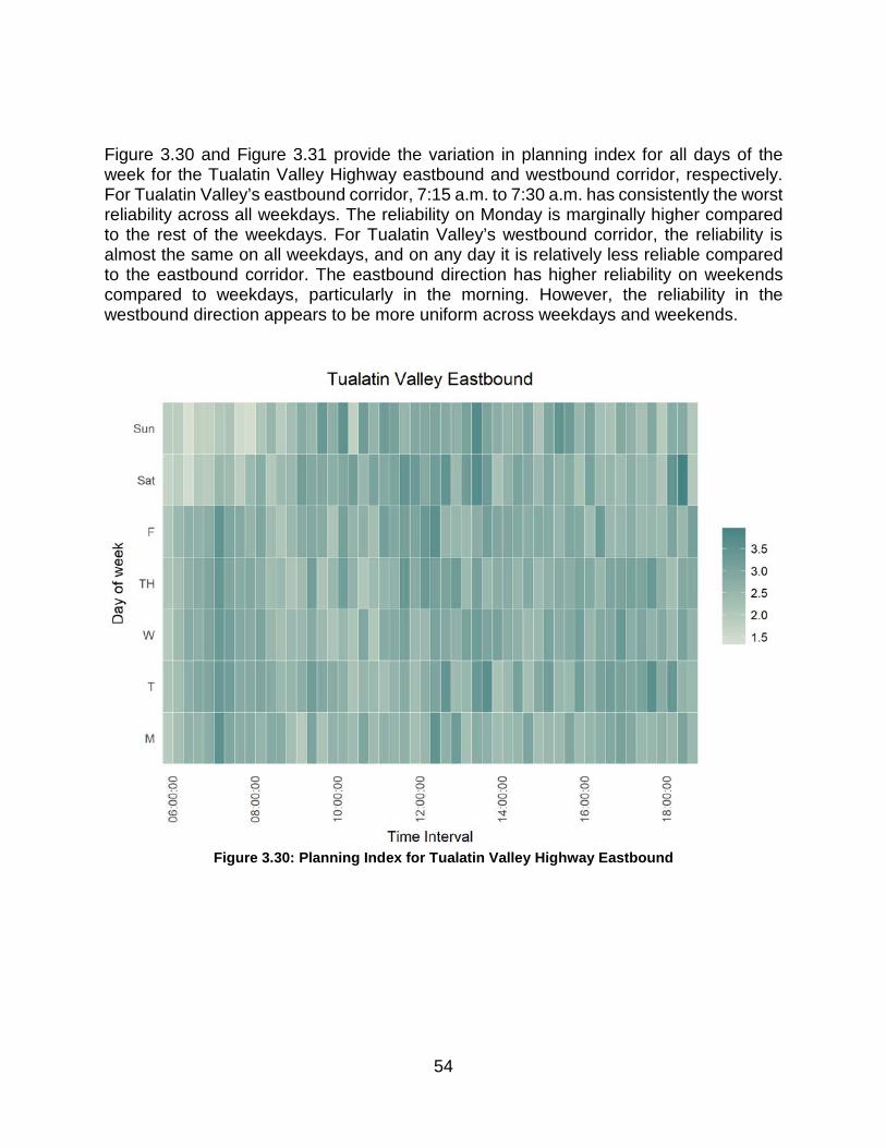
54

Figure 3.30 and Figure 3.31 provide the variation in planning index for all days of the week for the Tualatin Valley Highway eastbound and westbound corridor, respectively. For Tualatin Valley’s eastbound corridor, 7:15 a.m. to 7:30 a.m. has consistently the worst reliability across all weekdays. The reliability on Monday is marginally higher compared to the rest of the weekdays. For Tualatin Valley’s westbound corridor, the reliability is almost the same on all weekdays, and on any day it is relatively less reliable compared to the eastbound corridor. The eastbound direction has higher reliability on weekends compared to weekdays, particularly in the morning. However, the reliability in the westbound direction appears to be more uniform across weekdays and weekends.

Figure 3.30: Planning Index for Tualatin Valley Highway Eastbound

55

Figure 3.31: Planning Index for Tualatin Valley Highway Westbound

Figure 3.32 and Figure 3.33 provide the variation in planning index for all days of the week for Tualatin-Sherwood Road for the eastbound and westbound corridor, respectively. For Tualatin-Sherwood’s eastbound corridor during weekdays, Mondays have the highest reliability whereas Fridays have the lowest reliability. Weekday mornings have higher reliability in the eastbound and westbound directions. For the westbound corridor, the reliability is marginally higher on Fridays. Further, for the westbound corridor, the reliability appears to be higher on Friday and almost the same on the rest of the weekdays. The midday period appears to have the lowest reliability in the westbound direction, particularly from 11:15 a.m. to 11:30 a.m. Figure 3.32 and Figure 3.33 clearly show that weekends are more reliable than weekdays.

56

Figure 3.32: Planning Index for Tualatin-Sherwood Road Eastbound

57

Figure 3.33: Planning Index for Tualatin-Sherwood Road Westbound

Figure 3.34 and Figure 3.35 provide the variation in planning index for all days of the week for the OR 99W corridor for the eastbound and westbound corridors, respectively. For OR 99W, the northbound corridor has slightly higher reliability on Monday among the weekdays. For both the northbound and southbound directions, evening periods have the lowest reliability, with the lowest reliability period being more pronounced in the southbound direction. The reliability of the northbound corridor is higher compared to the southbound corridor.

58

Figure 3.34: Planning Index for OR 99W Northbound

59

Figure 3.35: Planning Index for OR 99W Southbound

To better understand travel times and their reliability, the existing travel time dataset is fused with the historical weather data obtained from CustomWeather2. This weather dataset has several weather attributes for each hour of a day, including temperature, weather descriptions, wind speed and direction, humidity, and visibility. Further, the weather condition descriptions include sunny, light rain, rain, fog and overcast, among others. The analysis is done to observe the variations in travel time and reliability when the weather changes from sunny to either rainy or foggy. 2 Custom Weather. Accessed at https://customweather.com/products/historical-data-analytics/

https://customweather.com/products/historical-data-analytics/

60

Table 3.22: Median Travel Time and Mean Planning Index During Different Weather Conditions

Corridor Direction Weather

Morning Midday Evening

Median PI Median PI Median PI

Tualatin Valley

Highway

EB Sunny 1006 2.72 996 2.84 1051 2.93

Not Sunny 1069 2.73 1001 2.78 1137 2.90

WB Sunny 884 2.61 973 3.33 1090 3.20

Not Sunny 871 2.47 949 2.88 1167 3.03


EB Sunny 778 3.70 988 4.89 871 3.98

Not Sunny 793 3.61 936 4.42 867 3.76

WB Sunny 686 3.81 822 4.94 921 4.06

Not Sunny 689 3.83 836 4.61 967 3.86

OR 99W

NB Sunny 347 1.89 362 2.10 413 2.39

Not Sunny 364 2.04 349 1.92 451 2.59

SB Sunny 326 1.97 344 2.27 448 2.77

Not Sunny 322 1.88 344 2.11 473 2.71

Table 3.22 present the median travel time and mean planning index of each corridor for different weather condition during the morning, midday and evening for weekdays. The table clearly shows that the effect of weather conditions does not have a significant effect on travel times and reliability. The effect is also varied. In some cases, there are slight increases in travel time with not-sunny weather, whereas an opposite effect is seen in other corridors. This is expected due to the timeframe of analysis, which is in the fall. We have not seen any extreme weather conditions which can affect the travel times during our time period of analysis. 3.4.2 Segment Level Analysis

In addition to the corridor=level analysis, we also compare the planning index of segments within each corridor for weekdays. The outliers for the segment-level data are filtered out using the procedure outlined in Section 3.2. Table 3.23 to Table 3.28 provide the mean planning index values for each segment within each corridor for morning, midday and evening periods individually.

61

From Table 3.23 and Table 3.24, segments 4 and 5 in the eastbound direction and 1 and 2 in the westbound direction (between Murray Boulevard and Lombard Avenue) have the lowest reliability, and segment 1 in the eastbound direction and 5 in the westbound direction (between Brookwood Avenue and Cornelius Pass Road) have the highest reliability. The segments between Murray Boulevard and Lombard Avenue are the shorter segments with a significantly high number of entrances and exits per mile compared to other segments. The reliability of these segments gets particularly worse in the evening time period. Note that the least reliable segments are those closest to OR 217 and Portland, and the most reliable segments are the farthest away from OR 217.

Table 3.23: Mean Planning Index for Each Segment of Tualatin Valley Hwy EB Segment

No. Start Location End Location Daily Average Morning Midday Evening

1 Tualatin Valley Hwy and Brookwood Ave


2.27 2.17 2.27 2.37

2 Tualatin Valley Hwy and Cornelius Pass Rd.

Tualatin Valley Hwy and 185th Ave 3.02 3.08 2.88 3.15


Tualatin Valley Hwy and Murray Blvd. 2.86 3 2.73 2.9


Tualatin Valley Hwy and Cedar Hills Blvd. 4.22 4.3 4.04 4.37


Canyon Rd. and Lombard Ave 4.04 3.27 4.21 4.62

Table 3.24: Mean Planning Index for Each Segment of Tualatin Valley Hwy WB Segment


1 Canyon Rd. and Lombard Ave

Tualatin Valley Hwy and Cedar Hills Blvd. 3.81 3.29 3.70 4.47


Tualatin Valley Hwy and Murray Blvd. 4.01 3.72 3.81 4.53


Tualatin Valley Hwy and 185th Ave 2.75 2.39 2.56 3.36



2.92 2.64 3.32 2.71

5 Tualatin Valley Hwy and Cornelius Pass Rd.

Tualatin Valley Hwy and Brookwood Ave 2.18 2.01 2.25 2.27

62

Table 3.25 and Table 3.26 provide the planning index values for each segment within Tualatin-Sherwood Road for the eastbound and westbound directions, respectively. The two short segments between Boones Ferry Road and I-5 have the worst reliability. For these segments, the travel time is particularly unreliable during the midday period. The segment between Langer Farms Parkway and Oregon Street have the highest reliability.

Table 3.25: Mean Planning Index for Each Segment of Tualatin-Sherwood EB Segment


1 Tualatin-Sherwood Rd. and OR 99W


4.63 4.11 4.70 5.07

2 Tualatin-Sherwood Rd. and Langer Farms Pkwy

Tualatin-Sherwood Rd. and Oregon St. 2.20 2.15 2.25 2.20


Tualatin-Sherwood Rd. and 124th Ave 3.38 3.49 3.29 3.37


Tualatin-Sherwood Rd. and Avery St. 3.58 3.49 3.60 3.64


Tualatin-Sherwood Rd. and Teton Ave 2.42 2.43 2.42 2.42



5.30 4.60 5.80 5.37



8.23 6.50 9.36 8.55


Nyberg St. and I-5 (SB On-Ramp) 6.70 5.33 7.71 6.81

Table 3.26: Mean Planning Index for Each Segment of Tualatin-Sherwood WB Segment


1 Nyberg St. and I-5 (SB On-Ramp)


6.62 5.88 7.03 6.85



6.23 6.04 6.21 6.43


Tualatin-Sherwood Rd. and Teton Ave 3.23 3.25 3.24 3.20


Tualatin-Sherwood Rd. and Avery St. 2.86 2.74 2.83 3.03


Tualatin-Sherwood Rd. and 124th Ave 4.50 3.46 4.49 5.56


Tualatin-Sherwood Rd. and Oregon St. 2.63 2.38 2.63 2.88

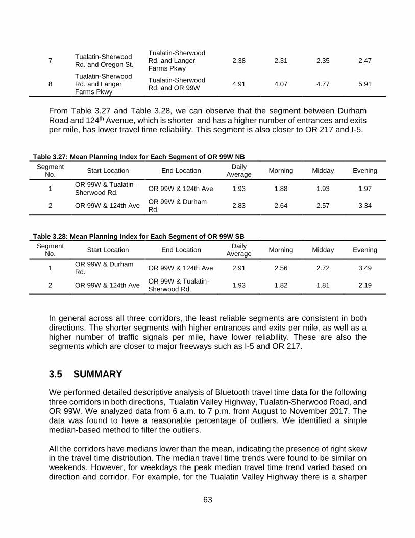
63



2.38 2.31 2.35 2.47

8 Tualatin-Sherwood Rd. and Langer Farms Pkwy

Tualatin-Sherwood Rd. and OR 99W 4.91 4.07 4.77 5.91

From Table 3.27 and Table 3.28, we can observe that the segment between Durham Road and 124th Avenue, which is shorter and has a higher number of entrances and exits per mile, has lower travel time reliability. This segment is also closer to OR 217 and I-5.

Table 3.27: Mean Planning Index for Each Segment of OR 99W NB Segment


1 OR 99W & Tualatin-Sherwood Rd. OR 99W & 124th Ave 1.93 1.88 1.93 1.97

2 OR 99W & 124th Ave OR 99W & Durham Rd. 2.83 2.64 2.57 3.34

Table 3.28: Mean Planning Index for Each Segment of OR 99W SB Segment


1 OR 99W & Durham Rd. OR 99W & 124th Ave 2.91 2.56 2.72 3.49

2 OR 99W & 124th Ave OR 99W & Tualatin-Sherwood Rd. 1.93 1.82 1.81 2.19

In general across all three corridors, the least reliable segments are consistent in both directions. The shorter segments with higher entrances and exits per mile, as well as a higher number of traffic signals per mile, have lower reliability. These are also the segments which are closer to major freeways such as I-5 and OR 217.

3.5 SUMMARY

We performed detailed descriptive analysis of Bluetooth travel time data for the following three corridors in both directions, Tualatin Valley Highway, Tualatin-Sherwood Road, and OR 99W. We analyzed data from 6 a.m. to 7 p.m. from August to November 2017. The data was found to have a reasonable percentage of outliers. We identified a simple median-based method to filter the outliers. All the corridors have medians lower than the mean, indicating the presence of right skew in the travel time distribution. The median travel time trends were found to be similar on weekends. However, for weekdays the peak median travel time trend varied based on direction and corridor. For example, for the Tualatin Valley Highway there is a sharper

64

morning peak and broader evening peak in the eastbound direction, and broader morning peak and a sharper evening peak in the westbound direction. For Tualatin-Sherwood, there is a sharp morning peak and broad peak covering midday and evening in the eastbound direction, and three peaks of increasing magnitude in the westbound direction. OR 99W has peak travel times in the evening period in both the northbound and southbound directions. There is a small morning peak observed in the northbound direction. We computed three different reliability metrics, buffer index, planning index, and normalized standard deviation. Tualatin Valley Highway, which is the longest corridor, has the highest mean and median travel time. Tualatin-Sherwood Road has the lowest reliability. For both Tualatin Valley and Tualatin-Sherwood, the eastbound direction has marginally higher median travel times as well as slightly higher reliability compared to the westbound direction. The OR 99W corridor has the lowest mean and median travel time and the highest reliability among the selected corridors. The northbound direction of OR 99W has marginally higher reliability than the southbound direction. In general, weekends and holidays were found to be more reliable than weekdays, which is expected. The morning period has the highest reliability for all three corridors across all time periods. The midday period is the least reliable for all three corridors during the weekends. For Tualatin-Sherwood Road, the midday period is the least reliable in both directions for both weekdays and weekends. During the weekdays for Tualatin Valley Highway, the evening period has the lowest travel time reliability for the eastbound direction, and the midday and evening period are the worst in terms of reliability for the westbound direction. For OR 99W, the evening period is the least reliable for weekdays. We can also see that the northbound direction of OR 99W has better reliability than the southbound direction for weekdays and weekends, with the difference being more pronounced for weekdays. Travel time reliability was found to have minor variations between weekdays for certain corridors. Mondays had marginally higher reliability for the northbound approach of the OR 99W corridor, and the Tualatin-Sherwood and Tualatin Valley eastbound corridors. Weather conditions were not found to have an impact on travel times and their reliability. However, during the timeframe of analysis, August to November 2017, there were no extreme weather events like snow or heavy rain. Therefore, we were unable to make any conclusions on the impact of weather on travel time reliability. We also compared the reliability of segments within each corridor. In general across all three corridors, the least reliable segments are consistent in both directions. The shorter segments with higher entrances and exits per mile, as well as higher number of traffic signals per mile, have lower reliability. These are also the segments which are closer to major freeways such as I-5 and OR 217.

65

4.0 FACTORS AND EFFECTS ON TRAVEL TIME AND TRAVEL TIME VARIABILITY

4.1 INTRODUCTION

In recent years, travel time reliability has worsened in the majority of urban areas of the United States, resulting in the need for drivers to plan for extra time to arrive at their destination on time. According to the most recent versions of the Urban Congestion Reports, the number of congested hours, travel time index, and planning time index all increased or remained the same from 2015 to 2016 (Federal Highway Administration, 2017a). Due to increases in congestion, it has been estimated that approximately three billion gallons of fuel and seven billion hours are consumed in traffic congestion each year (Schrank et al., 2015b). Increased travel times and variability in travel times due to congestion directly impact travelers and freight movements. Therefore, in an attempt to address these congestion-related issues, the Moving Ahead for Progress in the 21st Century Act (MAP-21) established national performance goals for system reliability that aimed to improve the efficiency of the surface transportation system (Federal Highway Administration, 2012). More specifically, in the Portland metro area (the location of the current study), congestions trends continue to worsen. In terms of population, the Portland area experienced an increase of 30,761 people from 2014 to 2015. From 2013 to 2015, this rise in population lead to a 13.6% increase in hours of weekday congestion and a 22.6% increase in the number of traffic delays (Oregon Department of Transportation, 2018b). These percentages are expected to increase, as forecasts show the Portland-area population is forecast to increase by 176,700 from 2015 to 2020. This was illustrated in a recent article, where Portland-area drivers were found to have spent 50 hours in peak-hour traffic in 2017, an increase of 6.4% over the previous year (Njus, 2018). In addition, using INRIX data, it was determined that approximately 20% of commute times are spent in congestion. Based on these statistics, the Portland area has the 12th-ranked worse traffic in the United States. As a result, it has been estimated that the time drivers spend in Portland-area traffic cost $3.9 billion per year due to fuel costs, costs due to lost time, and costs associated with freight delays (Njus, 2018). Due to increased congestion resulting in increased travel times and travel time variability, there have been numerous research efforts focusing on a variety of travel time concepts. Although some of these studies focus on arterials, the majority put their attention towards freeway travel times. Of the arterial-related work, areas of focus include travel time prediction, (Polus, 1979; Sen et al., 1996; Liu et al., 2006a; Liu et al., 2006b); travel time estimation (H. X. Liu and Ma, 2009; Chan et al., 2009; Hans et al., 2015; Skabardonis and Geroliminis, 2005); and travel time distribution (Hans et al., 2015; Chen et al., 2017; Zheng et al., 2017; Ramezani and Geroliminis, 2012; Yang et al., 2018). Although these works provide significant insights as it pertains to travel time on arterials, the effects of

66

specific factors on expected travel time and travel time standard deviation remain unknown. In light of this, the current study seeks to fill this gap in arterial travel time literature by identifying significant factors and quantifying their effects on travel time and travel time standard deviation on urban arterials. Due to potential correlation among unobservables for average travel time and travel time standard deviation (i.e., cross-equation correlation), the present study applies a bivariate econometric modeling approach to identify and quantify significant factors on expected travel time and travel time standard deviation. Based on data availability, specific factors included in model development are time-related variables (i.e., morning peak hours, evening peak hours, nighttime hours, and weekend peak hours); holidays (specific holidays that fall within the time frame used for analysis); weather conditions; and travel time and speed behavior in previous time intervals. Of the included variables, the following hypotheses are formed: Hypothesis 1

• Evening peak hours have the greatest positive effects on both average travel time and travel time standard deviation.

Hypothesis 2 • Nighttime hours have the greatest negative effects on average travel time and

travel time standard deviation.

Hypothesis 3 • Effects on average travel time and travel time standard deviation are significantly

different by direction.

4.2 RELATED WORK

The work in regards to travel time-related contexts is vast, varying from distribution fitting (Rahmani et al., 2015; Ma et al., 2017a; Fu et al., 2019; Ma et al., 2016; Westgate et al., 2016; Yang and Wu, 2016; Chalumuri and Yasuo, 2014; Guessous et al., 2014; Woodard et al., 2017); simulation-based studies (Chen and Chien, 2000; Ojeda-Cabral and Chorus, 2016; Zhang et al., 2018; Samandar, Williams, and Ahmed, 2018; Lv et al., 2019); and the value of travel time and travel time reliability (Athira et al., 2016; Truong and Hensher, 1985; Ettema and Timmermans, 2006; Devarasetty et al., 2012; Carrion and Levinson, 2012; Soriguera, 2014; Hensher, 2001; Engelson and Fosgerau, 2016; Kou et al., 2017; Xiao et al., 2017; Rich and Vandet, 2019; Bouscasse and Lapparent, 2019). However, of the travel time-related studies, the most related to the current work is travel time prediction or forecasting through various statistical methods. Hinsbergen et al. (2007) and Oh et al. (2015) summarize data-driven travel time prediction or forecasting methods into two distinct categories: parametric and nonparametric. As such, this section will review travel time prediction or forecasting studies based on these two categories.

67

4.2.1 Nonparametric

Of nonparametric methods in travel time research, many studies utilize neural network methods, Bayesian methods, or a combination of both. Park and Rilett (1998) conduct one of the earlier travel time studies using neural networks, in which modular artificial neural networks were used to forecast multiple-period freeway link travel times. One year later, Park and Rilett (1999) used a multilayer feedforward neural network model to forecast freeway link travel times. Focusing on the same freeway, Park et al. (1999) extended their previous studies to use a spectral basis neural network for real-time travel time forecasts. Palacharla and Nelson (1999) applied fuzzy logic and neural networks to dynamically estimate travel time on an arterial. For the freeway network of San Antonio, TX, Kisgyörgy and Rilett (2002) used a modular neural network to predict travel time using loop sensor and GPS data. Also focusing on freeway links, Dharia and Adeli (2003) applied a counter propagation neural network model to forecast freeway link travel times. Innamaa (2005) predicted freeway short-term travel times using a feedforward multilayer perceptron neural network model. Considering missing data by using data replacement schemes, Lint et al. (2005) utilized a state-space neural network to predict freeway travel times. Based off of a state-space neural network, Van Lint et al. (2007) predicted freeway travel time by modeling sate-space dynamics with a recurrent neural network. Khosravi et al. (2011b) applied a delta technique to construct prediction intervals for freeway travel times, as well as a genetic algorithm to automate neural network selection. To model freeway travel time, Zeng and Zhang (2013) applied a recurrent neural network model that considers temporal and spatial dynamics. Duan et al. (2016) used a deep learning model, LSTM neural network, to predict highway travel times in England. Wang et al. (2016) addressed spatial and autocorrelation in predicting travel times by applying a space- and time-delayed neural network model on a network in London. For a summary of neural network travel time studies, refer to Table 4.1. Table 4.1: Travel Time Studies Using Neural Networks

Study Method Roadway Type Park and Rilett (1998) • Clustering.

• Modular artificial neural network.

Freeway/Highway

Park and Rilett (1999) • Multilayer feedforward neural network.

Freeway/Highway

Park et al. (1999) • Spectral basis neural network

Freeway/Highway

Palacharla and Nelson (1999) • Fuzzy logit. • Neural network.

Arterial

You and Kim (2000) • Hybrid regression-based forecasting algorithm.

Network

Kisgyörgy and Rilett (2002) • Modular neural network. Freeway/Highway Dharia and Adeli (2003) • Counter propagation neural

network. Freeway/Highway

Innamaa (2005) • Feedforward multilayer perceptron neural network.

Freeway/Highway

Lint et al. (2005) • State-space neural network. Freeway/Highway

68

Lint et al. (2007) • State-space neural network. • Recurrent neural network.

Freeway/Highway

Khosravi et al. (2011b) • Delta technique. • Genetic algorithm. • Neural network.

Freeway/Highway

Zeng and Zhang (2013) • Recurrent neural network. Freeway/Highway Duan et al. (2016) • LSTM neural network. Freeway/Highway Wang et al. (2016) • Space- and time-delayed

neural network Network

The other most commonly used nonparametric approach for travel time prediction is the application of Bayesian methods. Van Hinsbergen and Van Lint (2008) used a Bayesian approach to combine multiple models to run in parallel. Utilizing a Bayesian pooling method, along with a fuzzy regression and a fusion algorithm, Choi and Chung (2009) estimated link travel time on urban networks. Van Hinsbergen et al. (2009) applied a Bayesian framework to both a state-space neural network and feedforward neural network to predict travel times on a highway in the Netherlands. Also using a Bayesian approach, Fei et al. (2011) utilized a Bayesian inference-based dynamic linear model to predict freeway travel times. Using both a Bayesian and delta method, Khosravi et al. (2011a) constructed prediction intervals for neural network forecasts of travel time. Liu et al. (2016) used an iterative Bayesian estimation approach to improve Bayesian fusion travel time estimates on urban arterials. Utilizing trip-based data and a Bayesian mixture model, Zhan et al. (2016) estimated travel times on an urban network. Working with various types of data, Mil and Piantanakulchai (2018) applied a Bayesian fusion approach and a Gaussian mixture model to estimate travel time while considering various traffic conditions. A summary of Bayesian-based methods is provided in Table 4.2. Table 4.2: Travel Time Studies Using Bayesian-based Methods

Study Method Roadway Type Hinsbergen and Lint (2008) • Bayesian framework with

multiple models. Freeway/Highway

Choi and Chung (2009) • Bayesian pooling. • Fuzzy regression. • Fusion algorithm.

Urban Network

Hinsbergen et al. (2009) • State-space and feedforward neural networks under a Bayesian framework.

Freeway/Highway

Fei et al. (2011) • Bayesian inference-based dynamic linear model.

Freeway/Highway

Khosravi et al. (2011a) • Bayesian and delta method with neural networks.

Freeway/Highway and Bus Route

Liu et al. (2016) • Iterative Bayesian fusion estimation.

Arterial

Zhan et al. (2016) • Bayesian mixture model. Urban Network Mil and Piantanakulchai (2018) • Bayesian fusion.

• Gaussian mixture model. Freeway/Highway

69

Although much of the nonparametric travel time prediction literature uses neural networks or Bayesian-based approaches, other nonparametric methods have been applied. Such examples include support vector regression (Wu et al., 2004), hazard-based duration models (Guo et al., 2011), and ensemble-based machine learning (Zhang and Haghani, 2015). 4.2.2 Parametric

As stated previously, parametric methods are the other approach that account for a variety of travel time prediction studies. Common parametric studies include the application of Kalman filtering, time-series models, and regression-based models. Of the parametric methods, much of the literature applies Kalman filtering methods. Chen and Chien (2001) used Kalman filtering to predict travel time on a freeway segment. A Kalman filtering approach was applied by Ming-sheng et al. (2002) to predict travel time on an urban expressway. Using automatic vehicle location data and automatic passenger counts, Shalaby and Farhan (2002) used Kalman filtering algorithms to predict bus travel times on an urban network. Chien and Kuchipudi (2003) utilized real-time and historical data, along with a Kalman filtering approach, to predict travel time on the New York State Thruway. Using a Kalman filtering algorithm, Chien et al. (2003) forecasted travel times for specific origin-destination pairs on New Jersey state highways. Kuchipudi and Chien (2003) developed a hybrid model, based on Kalman filtering, to predict travel times on the New York State Thruway. To predict travel time on arterials, Yang (2005a) applied a discrete-time Kalman filter under a special event scenario. Vanajakshi et al. (2009) used a Kalman filtering algorithm to predict bus travel times under heterogeneous traffic conditions on an urban network. Using Bluetooth data and ad hoc procedures, Barceló et al. (2010) applied Kalman filtering to predict travel time on freeways considering dynamic origin-destination estimation. Ji et al. (2010) applied a Kalman filtering method to dynamically predict travel time on a roadway in China. To compare prediction results for bus travel time on an urban network, Fan and Gurmu (2015) used Kalman filtering, historical average, and artificial neural network approaches. After organizing travel time data into clusters, Ladino et al. (2017) applied a Kalman filtering method to predict travel time on an arterial in France. Kumar et al. (2017) used a Kalman filtering approach to predict bus travel time using pattern trends and temporal discretization on an urban network. Using a spatial Kalman filtering method, Achar et al. (2019) predicted travel time and arrival time of buses on an urban network. Moonam et al. (2019) compared three methods, including Kalman filtering, to predict expected travel time on freeways. For a summary of travel time research using Kalman filtering techniques, refer to Table 4.3.

70

Table 4.3: Travel Time Studies Using Kalman Filtering Methods Study Method Roadway Type

Chen and Chien (2001) • Kalman filtering. Freeway/Highway Ming-sheng et al. (2002) • Kalman filtering. Freeway/Highway Shalaby and Farhan (2002) • Kalman filtering. Urban Network Chien and Kuchipudi (2003) • Kalman filtering. Freeway/Highway Chien et al. (2003) • Kalman filtering. Freeway/Highway Kuchipudi and Chien (2003) • Kalman filtering. Freeway/Highway Yang (2005a) • Kalman filtering. Arterials Vanajakshi et al. (2009) • Kalman filtering. Urban Network Barceló et al. (2010) • Kalman filtering.

• Ad hoc. Freeway/Highway

Ji et al. (2010) • Kalman filtering. Arterial Fan and Gurmu (2015) • Kalman filtering.

• Historical average model. • Artificial neural network.

Urban Network

Ladino et al. (2017) • Kalman filtering. • Clustering. • Best linear unbiased

estimation.

Arterial

Kumar et al. (2017) • Kalman filtering. Urban Network Achar et al. (2019) • Spatial Kalman filtering.

• State-space. Urban Network

Moonam et al. (2019) • Kalman filtering. • 𝑘𝑘-nearest neighbor. • Least squares regression

boosting.

Freeway/Highway

Another commonly used parametric method to predict or forecast travel time are time series analyses. Arem et al. (1997) applied a linear input-output ARMA (autoregressive moving average) model to predict travel time on freeway segments. D’Angelo et al. (1999) used a nonlinear SETAR (self-exciting threshold autoregressive) model, with single variable and multivariable prediction, to predict travel time on freeway corridors. Ishak and Al-Deek (2002) applied the nonlinear SETAR model proposed by D’Angelo et al. (1999) to evaluate its performance for short-term predictions on a freeway. Using a seasonal ARIMA (autoregressive integrated moving average) model, Williams and Hoel (2003) predicted travel time on freeways in both London and the United States. Yang (2005b) applied both an ARMA model and an ARIMA model to predict travel time along an arterial in Minnesota. Also using an ARIMA model, Billings and Yang (2006) predicted travel time on the same Minnesota arterial studied by Yang (2005b). Guin (2006), to predict freeway travel times in Georgia, applied a seasonal ARIMA model using historical travel time data. To forecast travel time variability on an urban network, Sohn and Kim (2009) applied the ARMA-GARCH (autoregressive moving average-generalized autoregressive conditional heteroscedasticity) model, where the ARMA and GARCH model are combined. In a spatial and temporal context, Reza et al. (2015) used an ARIMA model to forecast short-term travel time on a freeway due to a traffic incident. A summary of time series analyses for travel time prediction or forecasting is provided in Table 4.4.

71

Table 4.4: Travel Time Studies Using Time Series Analyses

Study Method Roadway Type Arem et al. (1997) • ARMA model. Freeway/Highway D’Angelo et al. (1999) • Nonlinear SETAR model. Freeway/Highway Ishak and Al-Deek (2002) • Nonlinear SETAR model. Freeway/Highway Williams and Hoel (2003) • Seasonal ARIMA model. Freeway/Highway Yang (2005b) • ARMA model.

• ARIMA model. Arterial

Billings and Yang (2006) • ARIMA model. Arterial Guin (2006) • Seasonal ARIMA model. Freeway/Highway Sohn and Kim (2009) • ARMA model.

• GARCH model. Urban Network

Reza et al. (2015) • ARIMA model. Freeway/Highway The final set of parametric approaches most observed in the travel time prediction literature are regression-based. In addition, these methods most relate to the proposed approach in the current study. Using a linear regression model, where coefficients vary as smooth functions of departure time, Zhang and Rice (2003) predicted short-term travel times on a freeway. Rice and Zwet (2004) also applied a linear regression approach with time-varying coefficients to predict travel time on freeways. Comparing tree-based methods and linear regression, Kwon et al. (2007) predicted travel time on freeways. In the context of bus arrival time, Bo et al. (2010) used linear regression and an adaptive algorithm to predict travel time as a means of predicting bus arrival time. Of the studies that most closely relate to the present study is the work of Martchouk et al. (2011), which applied a seemingly unrelated regression model to simultaneously estimate parameters on average travel time and travel time standard deviation. In doing so, Martchouk et al. identify specific factors that increase or decrease expected average travel time and travel time standard deviation. Jammula et al. (2018) used a linear regression model to predict travel time in mixed traffic conditions on an arterial, which was then compared to results of an arterial neural network. Using multivariate regression models, Rahman et al. (2018) estimated travel time on freeways. For a summary of regression-based travel time work, refer to Table 4.5. Table 4.5: Travel Time Studies Using Regression-based Analyses

Study Method Roadway Type Zhang and Rice (2003) • Linear regression with time-

varying coefficients. Freeway/Highway

Rice and Zwet (2004) • Linear regression with time-varying coefficients.

Freeway/Highway

Kwon et al. (2007) • Linear regression. • Tree-based methods.

Freeway/Highway

Bo et al. (2010) • Linear regression. • Adaptive algorithm.

Urban Network

Martchouk et al. (2011) • Seemingly unrelated regression.

Freeway/Highway

Jammula et al. (2018) • Linear regression. • Artificial neural network.

Arterial

72

Rahman et al. (2018) • Multivariate linear regression. Freeway/Highway As observed through the literature review, both nonparametric and parametric approaches have a primary focus of travel time on freeways or highways, with few studies focusing on arterials. In addition, although these works use various factors to predict travel time, quantitative effects of these factors are often not provided. For example, peak hours are known to increase expected travel times, but the measured effects (i.e., minutes and seconds) are unknown. Further, considering parametric approaches, the majority of regression-based studies apply basic linear regression models to predict travel time. With this in mind, the current study aims to uniquely fill these gaps in literature by focusing explicitly on travel time and arterials. On the parametric methodological side, to the best of the authors’ knowledge, the current study is the first to apply a bivariate Tobit model to simultaneously estimate average travel time and travel time standard deviation while accounting for the skewed distribution of travel time standard deviation. Lastly, the present work quantifies the effects of the predictor variables used through partial effects.

4.3 CORRIDOR AND TRAVEL TIME DATA

4.3.1 Corridor Selection

For the current study, four months of travel time data collected via Bluetooth detectors at select intersections on select corridors are used to identify significant factors affecting average interval travel times and their associated standard deviations. Being that the present work focuses on arterials, various potential arterials were considered for analysis. Upon investigation into potential corridors, five corridors were determined to have a large number of travel time records over a four-month period: August, September, October, and November of 2017. Of the five potential corridors, three were selected for analysis. The selected corridors, along with accompanying descriptions, are shown in Table 4.6.

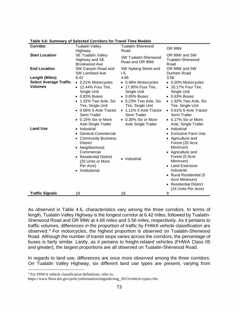
73

Table 4.6: Summary of Selected Corridors for Travel Time Models Corridor Tualatin Valley

Highway Tualatin-Sherwood Road OR 99W

Start Location SE Tualatin Valley Highway and SE Brookwood Ave

SW Tualatin-Sherwood Road and OR 99W

OR 99W and SW Tualatin-Sherwood Road

End Location SW Canyon Road and SW Lombard Ave

SW Nyberg Street and I-5

OR 99W and SW Durham Road

Length (Miles) 6.42 4.66 3.56 Select Average Traffic Volumes





Axle Single Trailer





Axle Single Trailer





Axle, Single Trailer Land Use • Industrial

• General Commercial • Community Business

District • Neighborhood

Commercial • Residential District

(25 Units or More Per Acre)

• Institutional

• Industrial

• Industrial • Exclusive Farm Use • Agriculture and

Forest (20 Acre Minimum)

• Agriculture and Forest (5 Acre Minimum)

• Land Extensive Industrial

• Rural Residential (5 Acre Minimum)

• Residential District (24 Units Per Acre)

Traffic Signals 18 18 8 As observed in Table 4.6, characteristics vary among the three corridors. In terms of length, Tualatin Valley Highway is the longest corridor at 6.42 miles, followed by Tualatin-Sherwood Road and OR 99W at 4.66 miles and 3.56 miles, respectively. As it pertains to traffic volumes, differences in the proportion of traffic by FHWA vehicle classification are observed.3 For motorcycles, the highest proportion is observed on Tualatin-Sherwood Road. Although the number of transit stops varies across the corridors, the percentage of buses is fairly similar. Lastly, as it pertains to freight-related vehicles (FHWA Class 05 and greater), the largest proportions are all observed on Tualatin-Sherwood Road. In regards to land use, differences are once more observed among the three corridors. On Tualatin Valley Highway, six different land use types are present, varying from 3 For FHWA vehicle classification definitions, refer to: https://www.fhwa.dot.gov/policyinformation/tmguide/tmg_2013/vehicle-types.cfm

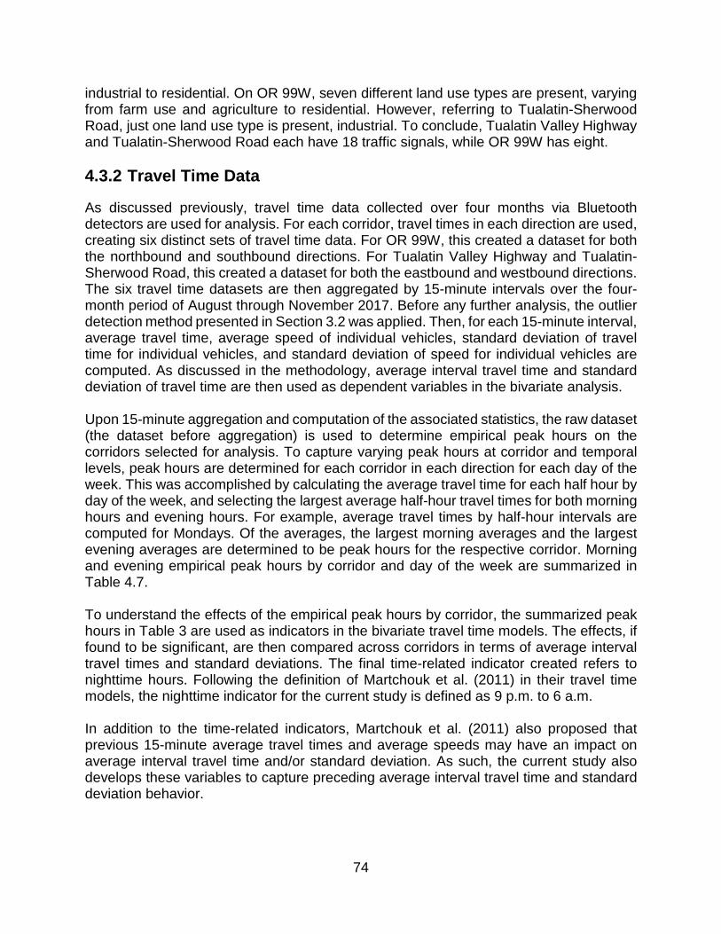
74

industrial to residential. On OR 99W, seven different land use types are present, varying from farm use and agriculture to residential. However, referring to Tualatin-Sherwood Road, just one land use type is present, industrial. To conclude, Tualatin Valley Highway and Tualatin-Sherwood Road each have 18 traffic signals, while OR 99W has eight. 4.3.2 Travel Time Data

As discussed previously, travel time data collected over four months via Bluetooth detectors are used for analysis. For each corridor, travel times in each direction are used, creating six distinct sets of travel time data. For OR 99W, this created a dataset for both the northbound and southbound directions. For Tualatin Valley Highway and Tualatin-Sherwood Road, this created a dataset for both the eastbound and westbound directions. The six travel time datasets are then aggregated by 15-minute intervals over the four-month period of August through November 2017. Before any further analysis, the outlier detection method presented in Section 3.2 was applied. Then, for each 15-minute interval, average travel time, average speed of individual vehicles, standard deviation of travel time for individual vehicles, and standard deviation of speed for individual vehicles are computed. As discussed in the methodology, average interval travel time and standard deviation of travel time are then used as dependent variables in the bivariate analysis. Upon 15-minute aggregation and computation of the associated statistics, the raw dataset (the dataset before aggregation) is used to determine empirical peak hours on the corridors selected for analysis. To capture varying peak hours at corridor and temporal levels, peak hours are determined for each corridor in each direction for each day of the week. This was accomplished by calculating the average travel time for each half hour by day of the week, and selecting the largest average half-hour travel times for both morning hours and evening hours. For example, average travel times by half-hour intervals are computed for Mondays. Of the averages, the largest morning averages and the largest evening averages are determined to be peak hours for the respective corridor. Morning and evening empirical peak hours by corridor and day of the week are summarized in Table 4.7. To understand the effects of the empirical peak hours by corridor, the summarized peak hours in Table 3 are used as indicators in the bivariate travel time models. The effects, if found to be significant, are then compared across corridors in terms of average interval travel times and standard deviations. The final time-related indicator created refers to nighttime hours. Following the definition of Martchouk et al. (2011) in their travel time models, the nighttime indicator for the current study is defined as 9 p.m. to 6 a.m. In addition to the time-related indicators, Martchouk et al. (2011) also proposed that previous 15-minute average travel times and average speeds may have an impact on average interval travel time and/or standard deviation. As such, the current study also develops these variables to capture preceding average interval travel time and standard deviation behavior.

75

Table 4.7: Empirical Peak Hours by Corridor and Day of the Week

Corridor Day of the Week Morning Peak Evening Peak Tualatin Valley Highway (Eastbound)

Monday 6:30 a.m. to 10:00 a.m.

2:30 p.m. to 6:00 p.m.

Tuesday 6:30 a.m. to 10:00 a.m.

3:00 p.m. to 6:30 p.m.

Wednesday 6:30 a.m. to 10:00 a.m.

2:00 p.m. to 6:00 p.m.

Thursday 6:30 a.m. to 10:30 a.m.

2:00 p.m. to 6:00 p.m.

Friday 6:30 a.m. to 11:00 a.m.

2:00 p.m. to 5:30 p.m.

Saturday 11:00 a.m. to 3:00 p.m. Sunday 12:00 p.m. to 4:00 p.m. Tualatin Valley Highway (Westbound)


3:00 p.m. to 6:00 p.m.


2:30 p.m. to 6:00 p.m.


3:00 p.m. to 6:00 p.m.


3:00 p.m. to 6:00 p.m.


3:00 p.m. to 6:00 p.m.

Saturday 12:30 p.m. to 4:00 p.m. Sunday 11:00 a.m. to 5:30 p.m. Tualatin-Sherwood Road (Eastbound)


2:00 p.m. to 5:30 p.m.


2:00 p.m. to 5:30 p.m.


2:00 p.m. to 5:30 p.m.


2:00 p.m. to 5:30 p.m.


2:00 p.m. to 5:30 p.m.

Saturday 11:30 a.m. to 2:30 p.m. Sunday 12:30 p.m. to 5:00 p.m. Tualatin-Sherwood Road (Westbound)


2:30 p.m. to 5:30 p.m.


3:00 p.m. to 6:00 p.m.


2:00 p.m. to 5:30 p.m.


2:00 p.m. to 5:30 p.m.


2:30 p.m. to 5:30 p.m.

Saturday 11:00 a.m. to 2:00 p.m.

76

Sunday 12:30 p.m. to 4:00 p.m. OR 99W (Northbound) Monday 6:30 a.m. to 10:30

a.m. 2:30 p.m. to 6:00 p.m.


2:30 p.m. to 6:00 p.m.


3:00 p.m. to 6:00 p.m.


2:30 p.m. to 6:00 p.m.


2:30 p.m. to 5:30 p.m.

Saturday 11:00 a.m. to 3:30 p.m. Sunday 12:00 p.m. to 3:30 p.m. OR 99W (Southbound Monday 6:30 a.m. to 10:30

a.m. 3:00 p.m. to 6:00 p.m.


3:00 p.m. to 6:00 p.m.


3:00 p.m. to 6:00 p.m.


3:00 p.m. to 6:00 p.m.


3:00 p.m. to 6:00 p.m.

Saturday 11:00 a.m. to 4:30 p.m. Sunday 12:30 p.m. to 4:30 p.m.

4.3.3 Weather Data

To better predict average interval travel times and travel time standard deviation, additional datasets with attributes that may impact travel time are explored. Of the datasets explored, the one dataset that could be fused with the raw format of the travel time data was historical weather data. Using weather data obtained from CustomWeather©, several weather attributes for each hour by day were merged with the travel time data. This was completed by generating a date index and time index in both datasets, in which the weather data could then be merged with the travel time data through these two indices. Of the weather attributes, the data included information on temperature, conditions (e.g., clear, overcast, rain, etc.), wind, and visibility. Leaving wind and visibility as continuous covariates for the bivariate analysis, the following weather condition indicators were created:

• Clear

• Sunny

77

• Foggy

• Rain and fog

• Light rain

4.4 METHODOLOGY

The purpose of the current study is to identify significant factors affecting average travel time and travel time variability and quantify their effects. As such, a bivariate modeling approach is applied. The choice of the bivariate analysis stems from potential cross-equation correlation among the error terms (i.e., correlation between unobservables related to average travel time and unobservables related to travel time standard deviation). By accounting for this cross-equation correlation, the efficiency of parameter estimations is improved (Greene, 2018; Cameron and Trivedi, 2005). In general, a seemingly unrelated regression (SUR) model would be appropriate in this context to simultaneously model average travel time and travel time standard deviation while accounting for cross-equation correlation and improving parameter efficiency. However, in using four months of travel time data and aggregating at 15-minute intervals, just one vehicle is observed for several 15-minute intervals over the four-month period considered. Subsequently, this results in a number of zero observations as it pertains to travel time standard deviation. Due to this potentially high number of zero observations, estimation of a SUR model would provide consistent estimates for the equation in which average travel time is the dependent variable, but would lead to inconsistent estimation of 𝜷𝜷 in the equation with travel time standard deviation as the dependent variable. To illustrate the number of zero observations in regards to travel time standard deviation, distributions of travel time standard deviation at 15-minute intervals by corridor are shown in Figure 4.1, Figure 4.2, and Figure 4.3.

In light of the presented distributions, an alternate modeling approach must be considered to account for the large number of zero observations regarding travel time standard deviation. For the current study, a bivariate Tobit modeling approach is used. The Tobit model (1958) is a censored regression or corner solution response model (Wooldridge, 2016; Cameron and Trivedi, 2005). The Tobit model allows the analyst to left- or right-censor at a given value to account for lower or upper thresholds. In the case of the current study, the left-censored value is zero.

78

Figure 4.1: Travel Time Standard Deviation Distribution on (a) OR 99W Northbound and (b) OR

99W Southbound

79

Figure 4.2: Travel Time Standard Deviation Distribution on (a) Tualatin-Sherwood Road Eastbound

and (b) Tualatin-Sherwood Road Westbound

80

Figure 4.3: Travel Time Standard Deviation Distribution on (a) Tualatin Valley Highway Eastbound

and (b) Tualatin Valley Highway Westbound

81

4.4.1 Bivariate Tobit Model

The bivariate Tobit model begins by defining two latent variables (Greene, 2016a; Trivedi and Zimmer, 2005): 𝑦𝑦𝑖𝑖𝑖𝑖∗ = 𝑿𝑿𝑖𝑖𝑖𝑖′ 𝜷𝜷𝑖𝑖 + 𝜀𝜀𝑖𝑖𝑖𝑖 , 𝑖𝑖 = 1, 2, … ,𝑁𝑁 and 𝑗𝑗 = 1, 2

𝑦𝑦𝑖𝑖𝑖𝑖 = �𝑦𝑦𝑖𝑖𝑖𝑖∗ if 𝑦𝑦𝑖𝑖𝑖𝑖∗ > 00 if 𝑦𝑦𝑖𝑖𝑖𝑖∗ ≤ 0

(4-1)

where 𝑦𝑦𝑖𝑖𝑖𝑖 is average interval travel time and travel time standard deviation (𝑗𝑗 = 1 for average interval travel time and 𝑗𝑗 = 2 for travel time standard deviation) for observation 𝑖𝑖, 𝑁𝑁 is the total number of observations, 𝜷𝜷𝑖𝑖 is a vector of parameters to be estimated, 𝑿𝑿𝑖𝑖𝑖𝑖′ is a vector of explanatory variables (e.g., peak-hour time, nighttime indicator, weather condition), and 𝜀𝜀𝑖𝑖𝑖𝑖 is a multivariate independently and normally distributed error term, such that: 𝜀𝜀𝑖𝑖~N�0,𝜎𝜎𝐽𝐽2,𝜌𝜌� (4-2)

with covariance matrix for a bivariate model:

� = �𝜎𝜎𝜀𝜀12 𝜌𝜌𝜀𝜀2𝜀𝜀1𝜎𝜎𝜀𝜀1

2 𝜎𝜎𝜀𝜀22

𝜌𝜌𝜀𝜀1𝜀𝜀2𝜎𝜎𝜀𝜀12 𝜎𝜎𝜀𝜀2

2 𝜎𝜎𝜀𝜀22 � (4-3)

where 𝜌𝜌 represents the correlation between error terms. If 𝜌𝜌 is statistically significant during estimation, there is significant cross-equation correlation and the bivariate approach is adequate. Based on the structure of the error terms (i.e., they are normally and independently distributed), the density function of 𝑦𝑦𝑖𝑖𝑖𝑖 has been shown to be (Trivedi and Zimmer, 2005; Greene, 2018):

𝑓𝑓𝑖𝑖�𝑦𝑦𝑖𝑖𝑖𝑖 | 𝑿𝑿𝑖𝑖𝑖𝑖′ 𝜷𝜷𝑖𝑖� = � �1 −Φ�𝑿𝑿𝑖𝑖𝑖𝑖′ 𝜷𝜷𝑖𝑖𝜎𝜎𝑖𝑖

��𝑦𝑦𝑖𝑖𝑖𝑖=0

� 𝜙𝜙�𝑦𝑦𝑖𝑖𝑖𝑖 − 𝑿𝑿𝑖𝑖𝑖𝑖′ 𝜷𝜷𝑖𝑖

𝜎𝜎𝑖𝑖�

𝑦𝑦𝑖𝑖𝑖𝑖>0

(4-4)

where Φ is the multivariate normal distribution function and 𝜙𝜙 is the multivariate normal density function. Using the density function, the bivariate Tobit log-likelihood function can be expressed using Olsen’s reparameterization transformation as follows (Olsen, 1978; Greene, 2016a):

82

𝐿𝐿𝐿𝐿 = � log �Φ �−𝑿𝑿𝑖𝑖1′ 𝜷𝜷1𝜎𝜎1

,− 𝑿𝑿𝑖𝑖2′ 𝜷𝜷2𝜎𝜎2

, 𝜌𝜌��𝑦𝑦1=0,𝑦𝑦2=0

+ � log ��1𝜎𝜎1�𝜙𝜙 �

𝑦𝑦1𝜎𝜎1− 𝑿𝑿𝑖𝑖1′ 𝜷𝜷1𝜎𝜎1

� �1 −Φ�𝛿𝛿 �𝑿𝑿𝑖𝑖2′ 𝜷𝜷2𝜎𝜎2

+ 𝜌𝜌𝜀𝜀1��𝑦𝑦1>0,𝑦𝑦2=0

+ � log ��1𝜎𝜎2�𝜙𝜙 �

𝑦𝑦2𝜎𝜎2− 𝑿𝑿𝑖𝑖2′ 𝜷𝜷2𝜎𝜎2

� �1 −Φ�𝛿𝛿 �𝑿𝑿𝑖𝑖1′ 𝜷𝜷1𝜎𝜎1

+ 𝜌𝜌𝜀𝜀2��𝑦𝑦1=0,𝑦𝑦2>0

+ � −log(2𝜋𝜋) + log𝑦𝑦1=1,𝑦𝑦2=1

�𝛿𝛿

𝜎𝜎1𝜎𝜎2− 2𝛿𝛿2(𝜀𝜀12 + 𝜀𝜀22 − 2𝜌𝜌𝜀𝜀1𝜀𝜀2)�

(4-5)

where 𝛿𝛿 is equal to 1 if 𝑦𝑦𝑖𝑖 is greater than zero, 𝛿𝛿 is equal to zero if 𝑦𝑦𝑖𝑖 is equal to zero, and all other terms have been defined previously. 4.4.2 Model Fit and Performance

To assess overall model fit, log-likelihood values computed via Eq. (5) are used to compute the Maddala 𝑅𝑅2 value. In previous work using Tobit models and/or their variants (i.e., bi- or multivariate), the Maddala 𝑅𝑅2 value has been shown to provide an adequate measure of the model’s fit (Anderson and Hernandez, 2017; Anastasopoulos, Tarko, and Mannering, 2008; Anastasopoulos, Mannering, et al., 2012; Anastasopoulos, Shankar, et al., 2012; Veall and Zimmerman, 1996). The Maddala 𝑅𝑅2 value is then computed as (Maddala, 1983):

𝑅𝑅2 = 1 − 𝑒𝑒�−2[𝐿𝐿𝐿𝐿(𝛽𝛽)−𝐿𝐿𝐿𝐿(0)]

𝑁𝑁 � (4-6) where 𝐿𝐿𝐿𝐿(𝛽𝛽) is the log-likelihood at convergence of the best fit model, 𝐿𝐿𝐿𝐿(0) is the log-likelihood at zero, and 𝑁𝑁 is the number of observations.

4.5 RESULTS AND DISCUSSION

To ease the presentation of results and discussion, each corridor will be presented and discussed individually by direction. Following the discussion of each corridor, a comparison of factors affecting average travel time and travel time standard deviation will be compared. 4.5.1 Results for OR 99W

4.5.1.1 Northbound

Best fit model specifications and effects on average travel time and travel time standard deviation on OR 99W (northbound) are shown in Table 4.8. As observed, the cross-

83

equation correlation term is significant with well over 99% confidence, indicating the bivariate approach is appropriate in this context. This suggests that there are correlated unobservables between average interval travel time and travel time standard deviation. In addition, with the cross-equation correlation terms being positive, the indirect effects of the correlated unobservables are increasing average interval travel time and travel time standard deviation. In other words, OR 99W may have both increasing average interval travel time and increasing travel time standard deviation due to commonly shared unobservables among the travel time metrics. Regarding significant indicators affecting average interval travel time various time-related indicators, holiday indicators, and average speed during the previous 15-minute intervals are found to be significant. Of the time-related indicators, four morning peak hours have significant effects on average interval travel time. Wednesday, Thursday, and Friday morning peak hours have approximately the same impact on average interval travel time, ranging from an expected increase, on average, of 23 seconds to 27 seconds. Tuesday morning peak hour has the largest impact on average interval travel time at an expected increase, on average, of 37 seconds. For evening peak hours, each day’s evening peak hours have significant effects on average interval travel time. The largest effects are observed on Tuesdays and Wednesdays, in which average interval travel time is expected to increase, on average, by one minute and 44 seconds. The time-related indicator with negative effects on average interval travel time is the indicator for nighttime (9 p.m. to 6 a.m.).4 Specifically, average interval travel time is expected to decrease, on average, by one minute and two seconds during these hours. Also with negative effects are the indicators for holidays, where average interval travel time on Labor Day and during Thanksgiving Day weekend are expected to decrease, on average, by 25 seconds and 26 seconds, respectively.5 In regards to the standard deviation equation, only time-related indicators are found to be significant, with just one having negative effects on travel time standard deviation. Of the time indicators with positive effects, Friday morning peak hour has the largest. Specifically, Friday morning peak hour is expected to increase, on average, travel time standard deviation by 13 seconds. The indicator with negative effects is the indicator for nighttime. According to estimations, nighttime hours are expected to decrease, on average, travel time standard deviation by 34 seconds.

4.5.1.2 Southbound

Best fit model specifications and effects on average interval travel time and travel time standard deviation on OR 99W (southbound) are shown in Table 4.9. Table 4.9 shows that the cross-equation correlation term is significant with well over 99% confidence, indicating the bivariate approach is appropriate in this context for OR 99W in the

4 As discussed previously, the definition of the nighttime indicator follows that of Martchouk et al. (2011). 5 With the 15-minute average travel time equation not having zero observations to censor, the effects are determined by the parameter estimations. In comparing Tobit estimations and OLS estimations of this regression equation, parameter estimates are identical. Regarding effects for the 15-minute standard deviation equation, an effects scale factor is computed based on the number of censored observations (Greene, 2016b).

84

southbound direction. As stated previously, this suggests that there are correlated unobservables between average interval travel time and travel time standard deviation. Referring to Table 4.9 and the 15-minute average travel time results, time-related indicators, holidays, and preceding average interval travel times are found to have significant effects. Regarding the time-related indicators, no morning peak hours are significant for the southbound direction of OR 99W. However, evening peaks for each weekday are found to be significant. Monday evening peak hour affects average interval travel time the least, as model estimations show that average interval travel times during Monday evening peak hour are expected, on average, to increase by one minute and 31 seconds. The remaining days of the week all have peak hours that increase average interval travel time, on average, by greater than two minutes. The evening peak hours with the largest effects are Thursday evening peak hour and Friday evening peak. Thursday evening peak hour is expected to increase average interval travel time, on average, by two minutes and 14 seconds, while Friday evening peak hour is expected to increase average interval travel time, on average, by two minutes and 19 seconds. As for weekend peak hours, just the Saturday peak hour is significant and is expected to increase average interval travel time, on average, by 30 seconds. The indicators with negative effects on average interval travel time are holidays. In particular, Labor Day is expected to decrease average interval travel time, on average, by 11 seconds and Thanksgiving Day weekend is expected to decrease average interval travel time, on average, by 17 seconds. For travel time standard deviation, two morning peak hours and all weekday evening peak hours are found to be significant. As it pertains to morning peak hours, the effects on travel time standard deviation are low compared to the effects of evening peak hours. For instance, Thursday and Friday morning peak hours are expected to increase average interval travel time, on average, by five seconds and four seconds, respectively. On the other hand, each evening peak hour is expected to increase average interval travel time by 10 seconds or greater, with the Monday evening peak hour having the largest impact at 18 seconds. With negative effects on travel time standard deviation are nighttime hours and Labor Day, where nighttime is expected to decrease travel time standard deviation, on average, by 42 seconds and Labor Day is expected to decrease travel time standard deviation, on average, by 13 seconds.

85

Table 4.8: Bivariate Tobit Model Specifications for OR 99W (Northbound) 𝒚𝒚𝟏𝟏 = 15-Minute Average Travel Time

Variable Coefficient Std. Error

Change in Travel Time

Constant 5.944a 0.026 Morning Peak Hours Tuesday (1 if 6:30 a.m. to 9:30 a.m., 0 Otherwise) 0.611a 0.038 + 37 sec Wednesday (1 if 6:30 a.m. to 11:00 a.m., 0 Otherwise) 0.421a 0.040 + 25 sec Thursday (1 if 6:30 a.m. to 11:00 a.m.) 0.448a 0.040 + 27 sec Friday (1 if 7:30 a.m. to 11:00 a.m., 0 Otherwise) 0.383a 0.078 + 23 sec Evening Peak Hours Monday (1 if 2:30 p.m. to 6:00 p.m., 0 Otherwise) 1.362a 0.040 + 1 min 22 sec Tuesday (1 if 3:30 p.m. to 6:00 p.m., 0 Otherwise) 1.731a 0.038 + 1 min 44 sec Wednesday (1 if 3:00 p.m. to 6:00 p.m., 0 Otherwise) 1.739a 0.043 + 1 min 44 sec Thursday (1 if 2:30 p.m. to 6:00 p.m., 0 Otherwise) 1.697a 0.034 + 1 min 42 sec Friday (1 if 2:30 p.m. to 5:30 p.m., 0 Otherwise) 1.437a 0.049 + 1 min 26 sec Weekend Peak Hours Saturday (1 if 11:00 a.m. to 3:30 p.m., 0 Otherwise) 0.488a 0.049 + 29 sec Off Peak Nighttime (1 if 9:00 p.m. to 6:00 a.m., 0 Otherwise) -1.026a 0.024 - 1 min 2 sec Holidays Labor Day (1 if Yes, 0 if No) -0.424a 0.078 - 25 sec Thanksgiving (1 if Yes, 0 if No) -0.430a 0.040 - 26 sec Speed 15-Minute Average Speed During Previous 15-Minute Time Period (mi/hr) -0.008a 0.001 - 0.5 sec

𝒚𝒚𝟐𝟐 = 15-Minute Travel Time Standard Deviation


Change in Standard Deviation

Constant 0.825a 0.012 Morning Peak Hours Friday (1 if 7:30 a.m. to 11:00 a.m., 0 Otherwise) 0.253a 0.036 + 13 sec Evening Peak Hours Monday (1 if 2:30 p.m. to 6:00 p.m., 0 Otherwise) 0.174a 0.042 + 9 sec Tuesday (1 if 3:30 p.m. to 6:00 p.m., 0 Otherwise) 0.191a 0.047 + 10 sec Wednesday (1 if 3:00 p.m. to 6:00 p.m., 0 Otherwise) 0.163a 0.051 + 8 sec Thursday (1 if 2:30 p.m. to 6:00 p.m., 0 Otherwise) 0.200a 0.044 + 10 sec Friday (1 if 2:30 p.m. to 5:30 p.m., 0 Otherwise) 0.114b 0.049 + 6 sec Weekend Peak Hours Saturday (1 if 11:00 a.m. to 3:30 p.m., 0 Otherwise) 0.209a 0.033 + 10 sec Sunday (1 if 12:00 p.m. to 3:30 p.m., Otherwise) 0.152a 0.033 + 8 sec Off Peak Nighttime (1 if 9:00 p.m. to 6:00 a.m., 0 Otherwise) -0.680a 0.018 - 34 sec Variances and Cross-Equation Correlation σ (15-Minute Average Travel Time) 0.778a 0.004 σ (15-Minute Standard Deviation) 0.675a 0.003 ρ (Cross-Equation Correlation) 0.473a 0.007 Model Summary Number of Observations 9,974 Log-Likelihood at Zero -24,708 Log-Likelihood at Convergence -20,525 Maddala R-Squared 0.57 a Significant at 99% Level of Confidence b Significant at 95% Level of Confidence

86

Table 4.9: Bivariate Tobit Model Specifications for OR 99W (Southbound) 𝒚𝒚𝟏𝟏 = 15-Minute Average Travel Time



Constant 4.970a 0.025 Evening Peak Hours Monday (1 if 3:00 p.m. to 6:00 p.m., 0 Otherwise) 1.515a 0.049 +1 min 31 sec Tuesday (1 if 3:00 p.m. to 6:00 p.m., 0 Otherwise) 2.150a 0.053 + 2 min 9 sec Wednesday (1 if 3:00 p.m. to 6:00 p.m., 0 Otherwise) 2.031a 0.056 + 2 min 2 sec Thursday (1 if 3:00 p.m. to 6:00 p.m., 0 Otherwise) 2.229a 0.055 + 2 min 14 sec Friday (1 if 3:00 p.m. to 6:00 p.m., 0 Otherwise) 2.313a 0.066 + 2 min 19 sec Weekend Peak Hours Saturday (1 if 11:00 a.m. to 4:30 p.m., 0 Otherwise) 0.493a 0.068 + 30 sec Off Peak Nighttime (1 if 9:00 p.m. to 6:00 a.m., 0 Otherwise) -0.640a 0.034 - 38 sec Holidays Labor Day (1 if Yes, 0 if No) -0.184b 0.093 - 11 sec Thanksgiving (1 if Yes, 0 if No) -0.287a 0.052 - 17 sec Preceding Travel Time 15-Minute Average Travel Time During Previous 15-Minute Time Period (mi/hr) 0.130a 0.003 + 8 sec




Constant 0.896a 0.016 Morning Peak Hours Thursday (1 if 7:00 a.m. to 11:00 a.m., 0 Otherwise) 0.103a 0.052 + 5 sec Friday (1 if 7:00 a.m. to 11:00 a.m., 0 Otherwise) 0.087c 0.051 + 4 sec Evening Peak Hours Monday (1 if 3:00 p.m. to 6:00 p.m., 0 Otherwise) 0.387a 0.066 + 18 sec Tuesday (1 if 3:00 p.m. to 6:00 p.m., 0 Otherwise) 0.226a 0.083 + 10 sec Wednesday (1 if 3:00 p.m. to 6:00 p.m., 0 Otherwise) 0.309a 0.079 + 14 sec Thursday (1 if 3:00 p.m. to 6:00 p.m., 0 Otherwise) 0.241a 0.085 + 11 sec Friday (1 if 3:00 p.m. to 6:00 p.m., 0 Otherwise) 0.279a 0.102 + 13 sec Weekend Peak Hours Saturday (1 if 11:00 a.m. to 4:30 p.m., 0 Otherwise) 0.269a 0.042 + 12 sec Sunday (1 if 12:30 p.m. to 4:30 p.m., Otherwise) 0.091b 0.045 + 4 sec Off Peak Nighttime (1 if 9:00 p.m to 6:00 a.m., 0 Otherwise) -0.905a 0.030 - 42 sec Holidays Labor Day (1 if Yes, 0 if No) -0.294b 0.135 - 13 sec Variances and Cross-Equation Correlation 𝜎𝜎 (15-Minute Average Travel Time) 0.957a 0.005 𝜎𝜎 (15-Minute Standard Deviation) 0.942a 0.004 𝜌𝜌 (Cross-Equation Correlation) 0.496a 0.006 Model Summary Number of Observations 9,577 Log-Likelihood at Zero -28,155 Log-Likelihood at Convergence -24,145 Maddala R-Squared 0.57 a Significant at 99% Level of Confidence b Significant at 95% Level of Confidence c Significant at 90% Level of Confidence

87

4.5.2 Results for Tualatin-Sherwood Road

4.5.2.1 Eastbound

Best fit model specifications and effects on average interval travel time and travel time standard deviation on Tualatin-Sherwood Road (eastbound) are shown in Table 4.10. As with the previous two models, the cross-equation correlation term is significant with well over 99% confidence, indicating the bivariate approach is appropriate in this context. As stated previously, this suggests that there are correlated unobservables between average interval travel time and travel time standard deviation. On Tualatin-Sherwood Road, in the eastbound direction, morning peak hours and evening peak hours for each day of the week are significant in regards to average interval travel time. For morning peak hours, the day with the smallest effects on average interval travel time is Monday and the largest is Friday. To be specific, Monday morning peak hour is expected to increase average interval travel time, on average, by one minute and one second, whereas Friday morning peak hour is expected to increase average interval travel time, on average, by two minutes and 22 seconds. During evening peak hours, all of which are found to be significant, the effects on average interval travel time are substantially larger compared to morning peak hours. For instance, four of the five peak hours (all days but Thursdays) result in an increase of average interval travel times of greater than three minutes. In particular, Monday peak hour is expected to increase average interval travel time, on average, by three minutes and 18 seconds; Tuesday peak hour (also the largest effect) is expected to increase average interval travel time, on average, by three minutes and 48 seconds; Wednesday peak hour is expected to increase average interval travel time, on average, by three minutes and 41 seconds; and, Friday peak hour is expected to increase average interval travel time, on average, by three minutes and 25 seconds. Of the indicators with negative effects are nighttime hours and holidays, each with varying effects on average interval travel time. Nighttime hours are expected to decrease average interval travel time by three minutes and seven seconds; Labor Day is expected to decrease average interval travel time by two minutes and 16 seconds; and Thanksgiving Day weekend is expected to decrease average interval travel time by one minute and 58 seconds. The time-related factors significant for travel time standard deviation are primarily morning peak hours, with one evening peak hour, weekend peak hours, and nighttime hours also significant. Of the morning peak hours, Wednesday and Friday morning peak hours have the largest effects on travel time standard deviation at an expected increase of 45 seconds and 52 seconds, respectively. The only significant evening peak hour is Monday, where travel time standard deviation is expected to increase by 31 seconds. The largest impact on travel time standard deviation are nighttime hours, which are expected to decrease travel time standard deviation by one minute and 25 seconds. Also resulting in an expected decrease in travel time standard deviation is Thanksgiving weekend, with an expected decrease of 26 seconds.

88

4.5.2.2 Westbound

Best fit model specifications and effects on average interval travel time and travel time standard deviation on Tualatin-Sherwood Road (westbound) are shown in Table 4.11. As with the previous three models, the cross-equation correlation term is significant with well over 99% confidence, indicating the bivariate approach is appropriate in this context for Tualatin-Sherwood Road in the westbound direction. As stated previously, this suggests that there are correlated unobservables between average interval travel time and travel time standard deviation. In regards to average interval travel time, both morning and evening peak hours for all days of the week are significant. Of the morning peak hours, Wednesday has the largest expected increase in average interval time at one minute and 47 seconds. The morning peak hour with the smallest impact on average interval travel time is Monday, with an expected increase of 53 seconds. For evening peak hours, the effects on travel time are markedly greater. Tuesday evening peak hour has the largest impact with an expected average interval travel time increase of five minutes and two seconds. Still, the remaining evening peak hours each have an expected increase in average interval travel time of greater than three minutes. Once more, nighttime hours and holidays have negative effects on average interval travel time. In particular, nighttime hours are expected to decrease average interval travel time by two minutes and 49 seconds; Labor day is expected to decrease average interval travel time by two minutes and eight seconds; and Thanksgiving Day weekend is expected to decrease average interval travel time by one minute and 36 seconds. For factors affecting travel time standard deviation, no evening peak hours are found to be significant; yet, four morning peak hours are significant. Of the four, Tuesday and Wednesday morning peak hours have the largest effects on travel time standard deviation at expected increases of 56 seconds and 59 seconds, respectively. For negative effects, the largest impact on travel time standard deviation are nighttime hours, with an expected decrease of one minute and 37 seconds. Table 4.10: Bivariate Tobit Model Specifications for Tualatin-Sherwood Road (Eastbound) 𝒚𝒚𝟏𝟏 = 15-Minute Average Travel Time



Constant 10.401a 0.089 Morning Peak Hours Monday (1 if 7:00 a.m. to 11:00 a.m., 0 Otherwise) 1.022a 0.200 + 1 min 1 sec Tuesday (1 if 7:00 a.m. to 11:00 a.m., 0 Otherwise) 1.925a 0.205 + 1 min 55 sec Wednesday (1 if 7:00 a.m. to 11:00 a.m., 0 Otherwise) 2.171a 0.184 + 2 min 10 sec Thursday (1 if 7:00 a.m. to 11:00 a.m., 0 Otherwise) 1.999a 0.209 + 2 min 0 sec Friday (1 if 7:30 a.m. to 11:00 a.m., 0 Otherwise) 2.359a 0.215 + 2 min 22 sec Evening Peak Hours Monday (1 if 2:00 p.m. to 5:30 p.m., 0 Otherwise) 3.304a 0.186 + 3 min 18 sec Tuesday (1 if 2:00 p.m. to 5:30 p.m., 0 Otherwise) 3.806a 0.179 + 3 min 48 sec Wednesday (1 if 2:00 p.m. to 5:30 p.m., 0 Otherwise) 3.679a 0.185 + 3 min 41 sec Thursday (1 if 2:00 p.m. to 5:30 p.m., 0 Otherwise) 2.904a 0.187 + 2 min 54 sec Friday (1 if 2:00 p.m. to 5:30 p.m., 0 Otherwise) 3.413a 0.177 + 3 min 25 sec

89

Weekend Peak Hours Saturday (1 if 11:30 a.m. to 2:30 p.m., 0 Otherwise) 1.350a 0.286 + 1 min 21 sec Off Peak Nighttime (1 if 9:00 p.m to 6:00 a.m., 0 Otherwise) -3.119a 0.119 - 3 min 7 sec Holidays Labor Day (1 if Yes, 0 if No) -2.259a 0.505 - 2 min 16 sec Thanksgiving (1 if Yes, 0 if No) -1.974a 0.252 - 1 min 58 sec Preceding Travel Time 15-Minute Average Travel Time During Previous 15-Minute Time Period (mi/hr) 0.199a 0.005 + 12 sec




Constant 1.612a 0.048 Morning Peak Hours Tuesday (1 if 7:00 a.m. to 11:00 a.m., 0 Otherwise) 0.944a 0.153 + 37 sec Wednesday (1 if 7:00 a.m. to 11:00 a.m., 0 Otherwise) 1.167a 0.156 + 45 sec Thursday (1 if 7:00 a.m. to 11:00 a.m., 0 Otherwise) 0.965a 0.171 + 37 sec Friday (1 if 7:30 a.m. to 11:00 a.m., 0 Otherwise) 1.342a 0.160 + 52 sec Evening Peak Hours Monday (1 if 2:00 p.m. to 5:30 p.m., 0 Otherwise) 0.798a 0.163 + 31 sec Weekend Peak Hours Saturday (1 if 11:30 a.m. to 2:30 p.m., 0 Otherwise) 0.624a 0.226 + 24 sec Sunday (1 if 12:30 p.m. to 5:00 p.m., Otherwise) 0.445b 0.182 + 17 sec Off Peak Nighttime (1 if 9:00 p.m. to 6:00 a.m., 0 Otherwise) -2.187a 0.086 - 1 min 25 sec Holidays Thanksgiving (1 if Yes, 0 if No) -0.668a 0.205 - 26 sec Variances and Cross-Equation Correlation 𝜎𝜎 (15-Minute Average Travel Time) 3.364a 0.022 𝜎𝜎 (15-Minute Standard Deviation) 2.843a 0.021 𝜌𝜌 (Cross-Equation Correlation) 0.378a 0.009 Model Summary Number of Observations 9,242 Log-Likelihood at Zero -44,962 Log-Likelihood at Convergence -41,947 Maddala R-Squared 0.48 a Significant at 99% Level of Confidence b Significant at 95% Level of Confidence

Table 4.11: Bivariate Tobit Model Specifications for Tualatin-Sherwood Road (Westbound) 𝒚𝒚𝟏𝟏 = 15-Minute Average Travel Time



Constant 10.396a 0.091 Morning Peak Hours Monday (1 if 7:30 a.m. to 11:00 a.m., 0 Otherwise) 0.878a 0.177 + 53 sec Tuesday (1 if 7:30 a.m. to 11:00 a.m., 0 Otherwise) 1.404a 0.260 + 1 min 24 sec Wednesday (1 if 7:30 a.m. to 11:00 a.m., 0 Otherwise) 1.784a 0.192 + 1 min 47 sec Thursday (1 if 7:30 a.m. to 11:00 a.m., 0 Otherwise) 1.673a 0.176 + 1 min 40 sec Friday (1 if 6:30 a.m. to 11:00 a.m., 0 Otherwise) 1.288a 0.172 + 1 min 17 sec Evening Peak Hours Monday (1 if 2:30 p.m. to 5:30 p.m., 0 Otherwise) 3.173a 0.178 + 3 min 10 sec Tuesday (1 if 3:00 p.m. to 6:00 p.m., 0 Otherwise) 5.039a 0.171 + 5 min 2 sec

90

Wednesday (1 if 2:00 p.m. to 5:30 p.m., 0 Otherwise) 3.762a 0.167 + 3 min 46 sec Thursday (1 if 2:00 p.m. to 5:30 p.m., 0 Otherwise) 3.897a 0.165 + 3 min 54 sec Friday (1 if 2:30 p.m. to 5:30 p.m., 0 Otherwise) 3.844a 0.189 + 3 min 51 sec Weekend Peak Hours Saturday (1 if 11:00 a.m. to 2:00 p.m., 0 Otherwise) 1.109a 0.202 + 1 min 7 sec Off Peak Nighttime (1 if 9:00 p.m to 6:00 a.m., 0 Otherwise) -2.810a 0.112 - 2 min 49 sec Holidays Labor Day (1 if Yes, 0 if No) -2.137a 0.495 - 2 min 8 sec Thanksgiving (1 if Yes, 0 if No) -1.596a 0.177 - 1 min 36 sec Preceding Travel Time 15-Minute Average Travel Time During Previous 15-Minute Time Period (mi/hr) 0.164a 0.005 + 10 sec




Constant 2.051a 0.048 Morning Peak Hours Tuesday (1 if 7:30 a.m. to 11:00 a.m., 0 Otherwise) 1.372a 0.168 + 56 sec Wednesday (1 if 7:30 a.m. to 11:00 a.m., 0 Otherwise) 1.464a 1.464 + 59 sec Thursday (1 if 7:30 a.m. to 11:00 a.m., 0 Otherwise) 1.107a 0.161 + 45 sec Friday (1 if 6:30 a.m. to 11:00 a.m., 0 Otherwise) 0.452a 0.168 + 18 sec Weekend Peak Hours Sunday (1 if 12:30 p.m. to 4:00 p.m., Otherwise) 0.647a 0.185 + 26 sec Off Peak Nighttime (1 if 9:00 p.m. to 6:00 a.m., 0 Otherwise) -2.390a 0.091 - 1 min 37 sec Holidays Thanksgiving (1 if Yes, 0 if No) -0.305c 0.164 - 12 sec Variances and Cross-Equation Correlation 𝜎𝜎 (15-Minute Average Travel Time) 3.302a 0.021 𝜎𝜎 (15-Minute Standard Deviation) 3.049a 0.021 𝜌𝜌 (Cross-Equation Correlation) 0.484a 0.007 Model Summary Number of Observations 9,491 Log-Likelihood at Zero -46,672 Log-Likelihood at Convergence -43,803 Maddala R-Squared 0.45 a Significant at 99% Level of Confidence c Significant at 90% Level of Confidence

4.5.3 Results for Tualatin Valley Highway

4.5.3.1 Eastbound

Best fit model specifications and effects on average interval travel time and travel time standard deviation on Tualatin-Sherwood Road (eastbound) are shown in Table 4.12. As with the previous four models, the cross-equation correlation term is significant with well over 99% confidence, indicating the bivariate approach is appropriate in this context for Tualatin Valley Highway in the eastbound direction. As stated previously, this suggests that there are correlated unobservables between average interval travel time and travel time standard deviation.

91

With respect to average interval travel time, morning peak hours and evening peak hours for each day of the week are significant. Along this corridor in this direction, Tuesday morning peak hour has the largest impact on average interval travel time at two minutes and 19 seconds. Wednesday morning peak hour, also with a larger impact on average interval travel time, is expected to increase average interval travel time by one minute and 59 seconds. The morning peak hour with the smallest impact is Friday, where Friday morning peak hour is expected to increase average interval travel time by 47 seconds. Of the evening peak hours, Tuesday again has the largest impact, as model estimations indicate Tuesday evening peak hour is expected to increase average interval travel time by two minutes and 55 seconds. The evening peak hour with the smallest impact is Monday with an expected increase in average interval travel time of one minute and 51 seconds. On this corridor, Saturday peak hour has a considerable impact on average interval travel time with an expected increase of one minute and 26 seconds. As with the previous models, nighttime hours and holidays result in an expected decrease in average interval travel time. Specifically, nighttime hours are expected to decrease average interval travel time by three minutes and 10 seconds; Labor Day is expected to decrease average interval travel time by two minutes and seven seconds; and Thanksgiving Day weekend is expected to decrease average interval travel time by one minute and 22 seconds. As it pertains to travel time standard deviation, morning peak hours for four days, nighttime hours, and Labor Day are the only significant factors. In regards to morning peak hours, Friday has the largest impact with an expected travel time standard deviation increase of 28 seconds and Monday has the smallest impact with an expected increase of 18 seconds. Nighttime hours and Labor Day, again, have negative effects on travel time standard deviation. As for nighttime hours, estimations indicate an expected decrease in travel time standard deviation of 50 seconds, while Labor Day is expected to decrease travel time standard deviation by 35 seconds.

4.5.3.2 Westbound

The sixth, and final, travel time model is for Tualatin Valley Highway in the westbound direction. Best fit model specifications and effects on average interval travel time and travel time standard deviation on Tualatin Valley Highway (westbound) are shown in Table 4.13. As with the previous five models, the cross-equation correlation term is significant with well over 99% confidence, indicating the bivariate approach is appropriate in this context for Tualatin Valley Highway in the westbound direction. Again, as stated previously, this suggests that there are correlated unobservables between average interval travel time and travel time standard deviation. For average interval travel time, no morning peak hours are significant and all evening peak hours are significant. Of the evening peak hours, Friday has the largest impact on average interval travel time with an expected increase of four minutes and 39 seconds. Also with a considerable impact is the Wednesday peak hour, as estimations show an expected increase of four minutes and 18 seconds. Again, as with the previous models, nighttime hours and holidays decrease expected travel time. Based on model estimations, nighttime hours are expected to decrease average interval travel time by two minutes and

92

41 seconds, while Labor Day is expected to decrease average interval travel time by one minute and 19 seconds. Travel time standard deviation for Tualatin Valley Highway in the eastbound direction had the fewest significant factors with three. The first is Sunday peak hour with an expected increase in travel time standard deviation of 16 seconds. The second is the indicator for nighttime hours and results in an expected decrease in travel time standard deviation of one minute and 18 seconds. The third is Labor Day and is expected to decrease travel time standard deviation by 54 seconds. Table 4.12: Bivariate Tobit Model Specifications for Tualatin Valley Highway (Eastbound) 𝒚𝒚𝟏𝟏 = 15-Minute Average Travel Time



Constant 15.418a 0.091 Morning Peak Hours Monday (1 if 6:30 a.m. to 10:00 a.m., 0 Otherwise) 1.103a 0.214 + 1 min 6 sec Tuesday (1 if 6:30 a.m. to 10:00 a.m., 0 Otherwise) 2.309a 0.201 + 2 min 19 sec Wednesday (1 if 6:30 a.m. to 10:00 a.m., 0 Otherwise) 1.977a 0.219 + 1 min 59 sec Thursday (1 if 6:30 a.m. to 10:30 a.m., 0 Otherwise) 1.587a 0.211 + 1 min 35 sec Friday (1 if 6:30 a.m. to 11:00 a.m., 0 Otherwise) 0.781a 0.266 + 47 sec Evening Peak Hours Monday (1 if 2:30 p.m. to 6:00 p.m., 0 Otherwise) 1.854a 0.250 + 1 min 51 sec Tuesday (1 if 3:00 p.m. to 6:30 p.m., 0 Otherwise) 2.917a 0.214 + 2 min 55 sec Wednesday (1 if 2:00 p.m. to 6:00 p.m., 0 Otherwise) 2.349a 0.235 + 2 min 21 sec Thursday (1 if 2:00 p.m. to 6:00 p.m., 0 Otherwise) 2.621a 0.213 + 2 min 37 sec Friday (1 if 2:00 p.m. to 5:30 p.m., 0 Otherwise) 2.216a 0.302 + 2 min 13 sec Weekend Peak Hours Saturday (1 if 11:00 a.m. to 3:00 p.m., 0 Otherwise) 1.427a 0.217 + 1 min 26 sec Off Peak Nighttime (1 if 9:00 p.m to 6:00 a.m., 0 Otherwise) -3.164a 0.108 - 3 min 10 sec Holidays Labor Day (1 if Yes, 0 if No) -2.120a 0.504 - 2 min 7 sec Thanksgiving (1 if Yes, 0 if No) -1.367a 0.207 - 1 min 22 sec Preceding Travel Time 15-Minute Average Travel Time During Previous 15-Minute Time Period (mi/hr) 0.056a 0.005 + 3 sec




Constant 0.436a 0.048 Morning Peak Hours Tuesday (1 if 6:30 a.m. to 10:00 a.m., 0 Otherwise) 0.566a 0.209 + 18 sec Wednesday (1 if 6:30 a.m. to 10:00 a.m., 0 Otherwise) 0.696a 0.252 + 22 sec Thursday (1 if 6:30 a.m. to 10:30 a.m., 0 Otherwise) 0.658a 0.210 + 21 sec Friday (1 if 6:30 a.m. to 11:00 a.m., 0 Otherwise) 0.892a 0.188 + 28 sec Off Peak Nighttime (1 if 9:00 p.m to 6:00 a.m., 0 Otherwise) -1.602a 0.095 - 50 sec Holidays Labor Day (1 if Yes, 0 if No) -1.115a 0.398 - 35 sec Variances and Cross-Equation Correlation 𝜎𝜎 (15-Minute Average Travel Time) 3.144a 0.020

93

𝜎𝜎 (15-Minute Standard Deviation) 2.748a 0.025 𝜌𝜌 (Cross-Equation Correlation) 0.238a 0.014 Model Summary Number of Observations 7,116 Log-Likelihood at Zero -31,386 Log-Likelihood at Convergence -29,995 Maddala R-Squared 0.32 a Significant at 99% Level of Confidence

Table 4.13: Bivariate Tobit Model Specifications for Tualatin Valley Highway (Westbound) 𝒚𝒚𝟏𝟏 = 15-Minute Average Travel Time



Constant 15.581a 0.105 Evening Peak Hours Monday (1 if 2:30 p.m. to 6:00 p.m., 0 Otherwise) 3.267a 0.260 + 3 min 16 sec Tuesday (1 if 3:00 p.m. to 6:30 p.m., 0 Otherwise) 3.432a 0.259 + 3 min 26 sec Wednesday (1 if 2:00 p.m. to 6:00 p.m., 0 Otherwise) 4.308a 0.264 + 4 min 18 sec Thursday (1 if 2:00 p.m. to 6:00 p.m., 0 Otherwise) 3.740a 0.275 + 3 min 44 sec Friday (1 if 2:00 p.m. to 5:30 p.m., 0 Otherwise) 4.654a 0.275 + 4 min 39 sec Weekend Peak Hours Saturday (1 if 11:00 a.m. to 3:00 p.m., 0 Otherwise) 1.295a 0.264 + 1 min 18 sec Off Peak Nighttime (1 if 9:00 p.m to 6:00 a.m., 0 Otherwise) -2.678a 0.127 - 2 min 41 sec Holidays Labor Day (1 if Yes, 0 if No) -1.319b 0.533 - 1 min 19 sec Thanksgiving (1 if Yes, 0 if No) -0.697a 0.240 - 42 sec Preceding Travel Time 15-Minute Average Travel Time During Previous 15-Minute Time Period (mi/hr) 0.039a 0.006 + 2 sec




Constant 0.463a 0.061 Weekend Peak Hours Sunday 0.557a 0.179 + 16 sec Off Peak Nighttime (1 if 9:00 p.m to 6:00 a.m., 0 Otherwise) -2.684a 0.137 - 1 min 18 sec Holidays Labor Day (1 if Yes, 0 if No) -1.842b 0.721 - 54 sec Variances and Cross-Equation Correlation 𝜎𝜎 (15-Minute Average Travel Time) 3.738a 0.029 𝜎𝜎 (15-Minute Standard Deviation) 3.546a 0.042 𝜌𝜌 (Cross-Equation Correlation) 0.250a 0.016 Model Summary Number of Observations 6,750 Log-Likelihood at Zero -30,886 Log-Likelihood at Convergence -29,840 Maddala R-Squared 0.27 a Significant at 99% Level of Confidence b Significant at 95% Level of Confidence

94

4.6 CORRIDOR COMPARISON

The following subsections compare significant factors by corridor and direction. Comparisons between morning peak hours, evening peak hours, weekend peak hours, nighttime hours, and holidays will be made. 4.6.1 Morning Peak Hours

For a comparison of morning peak hour effects on average interval travel time and travel time standard deviation, see Table 4.14 and Table 4.15. As shown in Table 4.14, morning peak hours have the least effects on OR 99W, as well as no significant effects in the southbound direction. Also with no significant effects in one direction is Tualatin Valley Highway, where no significant effects of morning peak hours are observed in the westbound direction. The largest effects, and each peak hour is significant in each direction, are observed on Tualatin-Sherwood Road. Tualatin-Sherwood Road is a primary arterial between Hillsboro, OR, and Beaverton, OR, then continues with a different name into Portland. The larger effects observed eastbound are likely explained by commuter traffic headed from Hillsboro to Beaverton or Portland. On Tualatin Valley Highway, the significance of morning peak hours in the eastbound direction may be explained by travelers exiting Interstate 5 to head east for work or the larger percentage of freight-related vehicles. For travel time standard deviation, just three morning peak hours are significant for OR 99W, one in the northbound direction (Friday) and two in the southbound direction (Thursday and Friday). On Tualatin Valley Highway, no westbound morning peak hours are significant and four of five eastbound morning peak hours are significant. Again, Tualatin-Sherwood Road has the most significant peak hours, with all morning peak hours, other than Monday, in each direction being significant. The greater variability on Tualatin-Sherwood Road is contingent on day of the week and direction. For example, standard deviation is expected to have a larger increase during the middle of the week in the westbound direction and a larger decrease in the eastbound direction on Friday.

Table 4.14: Comparison of Morning Peak Hour Effects on Average Interval Travel Time Corridor Direction Monday Tuesday Wednesday Thursday Friday OR 99W Northbound - ↑ 37 sec ↑ 25 sec ↑ 27 sec ↑ 23 sec

Southbound - - - - -

Tualatin-Sherwood Road Eastbound ↑ 61 sec

↑ 115 sec ↑ 130 sec ↑ 120

sec ↑ 142 sec

Westbound ↑ 53 sec ↑ 84 sec ↑ 107 sec ↑ 100

sec ↑ 77 sec

Tualatin Valley Highway Eastbound ↑ 66 sec

↑ 139 sec ↑ 119 sec ↑ 95 sec ↑ 47 sec

Westbound - - - - -

95

Table 4.15: Comparison of Morning Peak Hour Effects on Travel Time Standard Deviation

Corridor Direction Monday Tuesday Wednesday Thursday Friday

OR 99W Northbound - - - - ↑ 13 sec

Southbound - - - ↑ 5 sec ↑ 4 sec

Tualatin-Sherwood Road Eastbound - ↑ 37 sec ↑ 45 sec ↑ 37 sec ↑ 52

sec Westbound - ↑ 56

sec ↑ 59 sec ↑ 45 sec ↑ 18 sec

Tualatin Valley Highway Eastbound - ↑ 18 sec ↑ 22 sec ↑ 21 sec ↑ 28

sec Westbound - - - - -

4.6.2 Evening Peak Hours

For a comparison of evening peak hour effects on average interval travel time and travel time standard deviation, see Table 4.16 and Table 4.17. As anticipated, evening peak hours for each day in each direction are significant on all corridors. In general, the smallest increases are observed on OR 99W, although four evening peak hours in the southbound direction have considerable effects on average interval travel time. These increases might be explained by travelers electing to take OR 99W, rather than Interstate 5, to avoid more severe evening congested conditions on the interstate. In regards to Tualatin Valley Highway, larger effects on average interval travel time are observed in the westbound direction. This is likely a result of commuters who live outside of Portland and are commuting home after work. Lastly, there is Tualatin-Sherwood Road. In general, the directional difference is not as profound as Tualatin Valley Highway, where the largest differences by direction are on Tuesday and Thursday. The similar increases in average interval travel time may be explained by the arterial being a primary junction point to Interstate 5. Regarding travel time standard deviation, all evening peak hours in each direction are significant on OR 99W, with the greater variation being observed in the southbound direction. Considering travelers who elect to take OR 99W over Interstate 5, the difference in standard deviation may be capturing the associated traffic volumes. Of the other two corridors, Tualatin-Sherwood Road and Tualatin Valley Highway, just one peak hour on one corridor is significant in terms of travel time standard deviation. The significant peak hour is Monday on Tualatin-Sherwood Road in the eastbound direction.

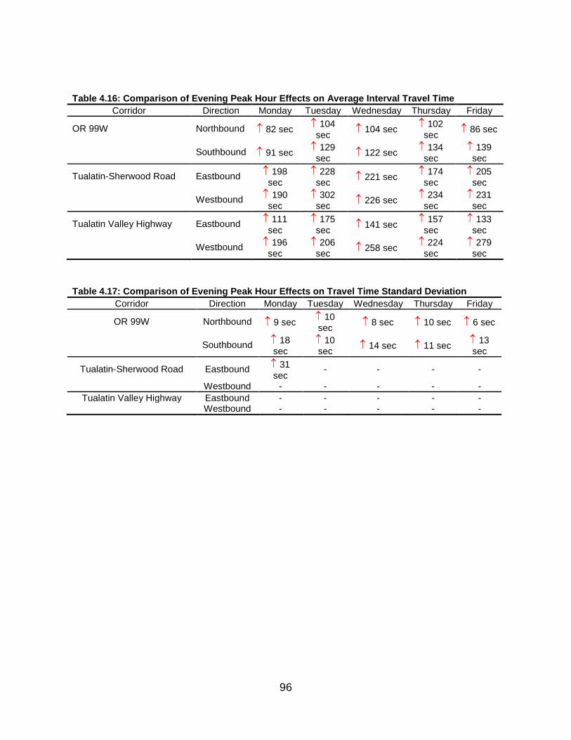
96

Table 4.16: Comparison of Evening Peak Hour Effects on Average Interval Travel Time


OR 99W Northbound ↑ 82 sec ↑ 104 sec ↑ 104 sec ↑ 102

sec ↑ 86 sec

Southbound ↑ 91 sec ↑ 129 sec ↑ 122 sec ↑ 134

sec ↑ 139 sec


↑ 228 sec ↑ 221 sec ↑ 174

sec ↑ 205 sec

Westbound ↑ 190 sec

↑ 302 sec ↑ 226 sec ↑ 234

sec ↑ 231 sec

Tualatin Valley Highway Eastbound ↑ 111 sec

↑ 175 sec ↑ 141 sec ↑ 157

sec ↑ 133 sec

Westbound ↑ 196 sec

↑ 206 sec ↑ 258 sec ↑ 224

sec ↑ 279 sec

Table 4.17: Comparison of Evening Peak Hour Effects on Travel Time Standard Deviation


OR 99W Northbound ↑ 9 sec ↑ 10 sec ↑ 8 sec ↑ 10 sec ↑ 6 sec

Southbound ↑ 18 sec

↑ 10 sec ↑ 14 sec ↑ 11 sec ↑ 13

sec


- - - - Westbound - - - - -

Tualatin Valley Highway Eastbound - - - - - Westbound - - - - -

97

4.6.3 Weekend Peak Hours

For a comparison of weekend peak hour effects on average interval travel time and travel time standard deviation, see Table 4.18 and Table 4.19. In terms of average interval travel time, no Sunday peak hour is found to be significant among the three corridors. However, Saturday peak hours in each direction on all corridors are significant. On OR 99W, the effects of Saturday peak hours are approximately the same in both directions. For the other two corridors, larger directional differences are observed. On Tualatin-Sherwood Road, the effects of Saturday peak hour are greater in the eastbound direction. Similar results are observed for Tualatin Valley Highway, in which the effects of Saturday peak hour are greater in the eastbound direction.

In regards to travel time standard deviation, Saturday peak is significant for two corridors: OR 99W and Tualatin-Sherwood Road. For OR 99W, the impact on standard deviation is approximately the same in both directions. On Tualatin-Sherwood Road, Saturday peak hour is significant in only the eastbound direction. As it pertains to Sunday peak hours, unlike average interval travel time, Sunday peak hour is significant across the three corridors. The largest effects on travel standard deviation are observed for Tualatin-Sherwood Road, where the larger impact occurs in the westbound direction. Sunday peak hour on Tualatin Valley Highway is found to be significant in only the westbound direction.

Table 4.18: Comparison of Weekend Peak Hour Effects on Average Interval Travel Time

Corridor Direction Saturday Sunday OR 99W Northbound ↑ 29 sec -

Southbound ↑ 30 sec - Tualatin-Sherwood Road Eastbound ↑ 81 sec -

Westbound ↑ 67 sec - Tualatin Valley Highway Eastbound ↑ 86 sec -

Westbound ↑ 78 sec -

Table 4.19: Comparison of Weekend Peak Hour Effects on Travel Time Standard Deviation

Corridor Direction Saturday Sunday OR 99W Northbound ↑ 10 sec ↑ 8 sec

Southbound ↑ 12 sec ↑ 4 sec Tualatin-Sherwood Road Eastbound ↑ 24 sec ↑ 17 sec

Westbound - ↑ 26 sec Tualatin Valley Highway Eastbound - -

Westbound - ↑ 16 sec

98

4.6.4 Nighttime Hours

For a comparison of nighttime hours effects on average interval travel time and travel time standard deviation, see Table 4.20 and Table 4.21. As shown, nighttime hours substantially decrease the expected average interval travel times on each corridor in each direction. On OR 99W, the greater decrease is observed in the northbound direction at 62 seconds (compared to 38 seconds in the southbound direction). On Tualatin-Sherwood Road, the eastbound direction has a lower expected travel time compared to the westbound direction (187 seconds to 169 seconds). Nighttime hours on Tualatin Valley Highway also have a greater impact in the eastbound direction, as average interval travel time is expected to decrease by 190 seconds (compared to 161 seconds in the westbound direction). In regards to standard deviation, nighttime hours substantially decrease the travel time standard deviation on each corridor in each direction. However, compared to average interval travel times, the opposite direction experiences the larger expected decrease in travel time standard deviation. For instance, OR 99W southbound has an expected decrease in travel time standard deviation of 42 seconds, compared to 34 seconds in the northbound direction. On Tualatin-Sherwood Road, the greater impact is experienced in the westbound direction, with an expected decrease of 97 seconds. Lastly, on Tualatin Valley Highway, the greater impact is also experienced in the westbound direction, where travel time standard deviation is expected to decrease by 78 seconds.

Table 4.20: Comparison of Nighttime Hour Effects on Average Interval Travel Time

Corridor Direction Nighttime Hours (9:00 p.m. to 6:00 a.m.) OR 99W Northbound ↓ 62 sec

Southbound ↓ 38 sec Tualatin-Sherwood Road Eastbound ↓ 187 sec

Westbound ↓ 169 sec Tualatin Valley Highway Eastbound ↓ 190 sec

Westbound ↓ 161 sec

Table 4.21: Comparison of Nighttime Hours Effects on Travel Time Standard Deviation

Corridor Direction Nighttime Hours (9:00 p.m. to 6:00 a.m.) OR 99W Northbound ↓ 34 sec Southbound ↓ 42 sec Tualatin-Sherwood Road Eastbound ↓ 85 sec Westbound ↓ 97 sec Tualatin Valley Highway Eastbound ↓ 50 sec

Westbound ↓ 78 sec

99

4.6.5 Holidays

For a comparison of holiday effects on average interval travel time and travel time standard deviation, see Table 4.22 and Table 4.23. In regards to average interval travel time, holidays decrease the expected average interval travel time on each corridor in each direction. On OR 99W, the holiday effects are fairly similar by holiday and direction. On Tualatin-Sherwood Road, the effects on the eastbound direction are greater. For Labor Day, the decrease in expected average interval travel time is 136 seconds (compared to 128 seconds in the westbound direction). For Thanksgiving weekend, the decrease in expected average interval travel time is 118 seconds (compared to 96 seconds in the westbound direction). The same trend is true for Tualatin Valley Highway, in which the decrease in expected average interval travel time are substantially greater in the eastbound direction. As for travel time standard deviation, the results are varied. On OR 99W, only Labor Day and in the southbound direction has significance. On Tualatin-Sherwood Road, Thanksgiving weekend is significant, while Labor Day is not. In addition, the difference in the decrease in expected average interval travel times is 14 seconds between eastbound and westbound directions. For Tualatin Valley Highway, the only significant effects occur on Labor Day. Specifically, Labor Day is expected to decrease the average interval travel time in the eastbound direction by 35 seconds, whereas the westbound direction is expected to experience a decrease of 54 seconds.

Table 4.22: Comparison of Holiday Effects on Average Interval Travel Time

Corridor Direction Labor Day Thanksgiving OR 99W Northbound ↓ 25 sec ↓ 26 sec Southbound ↓ 11 sec ↓ 17 sec Tualatin-Sherwood Road Eastbound ↓ 136 sec ↓118 sec Westbound ↓ 128 sec ↓ 96 sec Tualatin Valley Highway Eastbound ↓ 127 sec ↓ 82 sec

Westbound ↓ 79 sec ↓ 42 sec

Table 4.23: Comparison of Holiday Effects on Travel Time Standard Deviation

Corridor Direction Labor Day Thanksgiving OR 99W Northbound - - Southbound ↓ 13 sec - Tualatin-Sherwood Road Eastbound - ↓ 26 sec Westbound - ↓ 12 sec Tualatin Valley Highway Eastbound ↓ 35 sec - Westbound ↓ 54 sec -

100

4.7 SUMMARY AND CONCLUSIONS

Using four months of travel time data collected via Bluetooth detectors, average travel time and travel time standard deviation on urban arterials were analyzed. The empirical data was used to identify empirical peak hours, then aggregated at 15-minute intervals and merged with weather data. Using the merged dataset, various indicators were created to identify and quantify the effects on average interval travel time and travel time standard deviation. Due to the aggregation procedure, and the nature of the dependent variable, a bivariate modeling approach was applied. In doing so, the current study addresses the gaps in literature by focusing exclusively on arterials, applying a previously unused parametric method, and quantifies the effects of specific variables on average interval travel time and travel time standard deviation. Though the bivariate Tobit model, correlation among unobservables related to average interval travel time and standard deviation (i.e., cross-equation correlation) have been accounted for. In addition, the large number of zero observations as it pertains to travel time standard deviation have been addressed. For each model, the correlation coefficient is found to be significant with well over 99% confidence, indicating the bivariate approach is adequate and preferred in this context. From model estimations, several characteristics were found to statistically impact expected average interval travel time and travel time standard deviation, including morning peak hours, evening peak hours, weekend peak hours, nighttime hours, holidays, and speed or travel time behavior in the preceding 15-minute period. Using model estimations and effects from the aforementioned indicators, Hypothesis 1 to Hypothesis 3 can be answered. Hypothesis 1 Evening peak hours have the greatest effects on expected increases in average interval travel time, but do not have the greatest effects on expected increases in travel time standard deviation. On that premise, Hypothesis 1 is rejected. Similar, or greater, increases in travel time standard deviation are observed during morning peak hours and evening peak hours. Hypothesis 2 Nighttime hours have the greatest negative effects (i.e., decreases) on average interval travel time and travel time standard deviation. Therefore, the authors fail to reject Hypothesis 2. This is plausible, as traffic volumes are substantially lower during the hours of 9 p.m. to 6 a.m. Lower traffic volumes will decrease average interval travel times due to decreases in the likelihood of encountering congestion. In addition, due to lower traffic volumes, incidents along the roadway (e.g., crash, work-zone, etc.) are likely to have less of an impact on travel time and travel time variability. Hypothesis 3 For cases in which there was more than one observation, a two-sample 𝑡𝑡-test was conducted to determine if there is any statistical difference of effects by direction. In

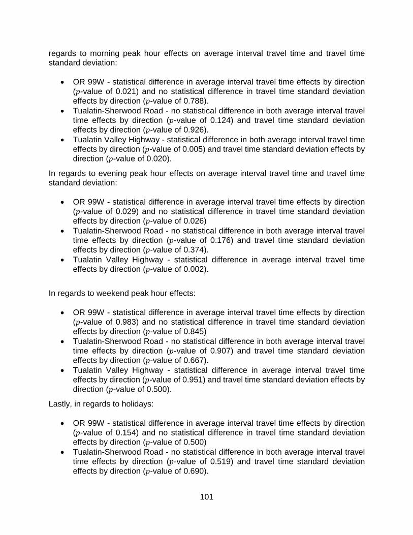
101

regards to morning peak hour effects on average interval travel time and travel time standard deviation:

• OR 99W - statistical difference in average interval travel time effects by direction (𝑝𝑝-value of 0.021) and no statistical difference in travel time standard deviation effects by direction (𝑝𝑝-value of 0.788).

• Tualatin-Sherwood Road - no statistical difference in both average interval travel time effects by direction (𝑝𝑝-value of 0.124) and travel time standard deviation effects by direction (𝑝𝑝-value of 0.926).

• Tualatin Valley Highway - statistical difference in both average interval travel time effects by direction (𝑝𝑝-value of 0.005) and travel time standard deviation effects by direction (𝑝𝑝-value of 0.020).

In regards to evening peak hour effects on average interval travel time and travel time standard deviation:

• OR 99W - statistical difference in average interval travel time effects by direction (𝑝𝑝-value of 0.029) and no statistical difference in travel time standard deviation effects by direction (𝑝𝑝-value of 0.026)


• Tualatin Valley Highway - statistical difference in average interval travel time effects by direction (𝑝𝑝-value of 0.002).

In regards to weekend peak hour effects:



• Tualatin Valley Highway - statistical difference in average interval travel time effects by direction (𝑝𝑝-value of 0.951) and travel time standard deviation effects by direction (𝑝𝑝-value of 0.500).

Lastly, in regards to holidays:



102

• Tualatin Valley Highway - statistical difference in average interval travel time effects by direction (𝑝𝑝-value of 0.274) and travel time standard deviation effects by direction (𝑝𝑝-value of 0.800).

Considering that each corridor analyzed in the current study has essentially the same traffic volumes, yet effects of time-related factors are shown to be substantially different in some cases, lessons can be learned from a policy and practice perspective. The corridor that experienced the greatest increase in expected travel times is a segment connecting an interstate and a principal arterial.

103

5.0 SUMMARY

The presented work presents various applications to understand travel time and related factors. Items include a detailed literature review on travel time reliability metrics; corridor selection and associated descriptive statistics; outlier detection and removal; median travel time analysis; descriptive statistics on travel time reliability metrics; and a modeling framework to identify significant factors and quantify their effects on average travel time and travel time standard deviation.

The literature review revealed that travel time reliability measures quantifies the variability in travel times, where performance metrics are broadly categorized by the following groups: Statistical Range, Buffer Time, and Tardy Trip Indicators. It was discovered that a single, consistently used reliability metric has not been agreed upon; therefore, computing and assessing various metrics is appropriate. However, FHWA does recommend a series of travel time reliability metrics, in which these metrics were adopted for the current study. It was also determined that arterial-focused travel time research is sparse when compared to freeway-based travel time research.

For the travel time analysis, three corridors in Washington County were selected based on their average traffic volumes and data availability: OR 99W, Tualatin-Sherwood Road, and Tualatin Valley Highway. The time period considered for analysis, due to the number of travel time observations, was August to November 2017. Each corridor was divided into segments based on the location of Bluetooth detectors, as to analyze each at the corridor level as well as the segment level. It was found that each corridor, although having similar average traffic volumes, has varying aspects that may impact travel time. Differences among corridors include land use, number of traffic signals, transit stops, number of entrances and exits, and percentage of freight-related vehicles. Before any analyses on the travel time data were to take place, an outlier detection method was adopted to identify and remove invalid travel times. Being that traffic conditions were found to differ by weekdays, weekends and holidays, the travel time data was filtered into these three distinct datasets. The outlier detection method was then applied to each dataset independently. Based on visual inspection, the outlier detection method appears to be successful in identifying erroneous travel time records. Upon outlier removal, the change in travel time statistics were assessed. This resulted in an increase in average speed and 15th percentile travel times, while all other metrics decreased (e.g., average travel time, median travel time, travel time standard deviation, etc.). Using the datasets with outliers removed, a median travel time analysis was conducted. This was done by analyzing five-minute median travel times for weekdays, weekends and holidays. With the majority of travel time records being between 6 a.m. and 7 p.m., the focus of the median travel time analysis was on travel time records within this time period. In addition, the median travel time analysis was further disaggregated to analyze travel times during the morning (6 a.m. to 10 a.m.), during midday (10 a.m. to 3 p.m.), and during the evening (3 p.m. to 7 p.m.). It was found that all corridors have medians lower than the mean, indicating the travel time distributions are right-skewed. On weekends, all corridors

104

were found to have similar median travel time trends. However, on weekdays, peak median travel times varied by corridor and direction. As it pertains to statistics on travel time reliability metrics, the buffer index, planning index, and normalized standard deviation were presented. These metrics indicate that Tualatin-Sherwood Road has the lowest travel time reliability of the three corridors. It was also found that the westbound directions of Tualatin Valley Highway and Tualatin-Sherwood Road have slightly higher reliability compared to their westbound directions. Of the selected corridors, OR 99W has the highest reliability, where the northbound is slightly more reliable than the southbound direction. In terms of time of day, mornings have the highest reliability and midday on weekends has the lowest reliability for all three corridors. At the segment level, shorter segments with a large number of entrances and exits have the lowest reliability. Through a bivariate modeling framework, significant factors on average travel time and travel time standard deviation were determined. In addition to determining such factors, their effects on average travel time and travel time standard deviation were quantified. Of the various methods to model travel time, the current work adopts a bivariate Tobit model to account for cross-equation correlation and the large number of zero observations for travel time standard deviation. Factors including morning peak hours, evening peak hours, weekend peak hours, and nighttime hours were found to be significant and have moderate to considerable effects on average travel time and travel time standard deviation. For nearly all factors, the largest effects (both positive and negative) on average travel time and travel time standard deviation are observed on Tualatin-Sherwood Road.

105

6.0 REFERENCES

Achar, Avinash, Dhivya Bharathi, Bachu Anil Kumar, and Lelitha Vanajakshi. 2019. Bus Arrival Time Prediction : A Spatial Kalman Filter Approach. IEEE Transactions on Intelligent Transportation Systems, 1-10. https://doi.org/10.1109/TITS.2019.2909314.

Anastasopoulos, Panagiotis Ch., Fred L. Mannering, Venky N. Shankar, and John E. Haddock. 2012. A Study of Factors Affecting Highway Accident Rates Using the Random-Parameters Tobit Model. Accident Analysis and Prevention 45, pp. 628–633.

Anastasopoulos, Panagiotis Ch., Venky N. Shankar, John E. Haddock, and Fred L. Mannering. 2012. A Multivariate Tobit Analysis of Highway Accident-Injury-Severity Rates. Accident Analysis and Prevention 45, pp. 110–119.

Anastasopoulos, Panagiotis Ch., Andrew P. Tarko, and Fred L. Mannering. 2008. Tobit Analysis of Vehicle Accident Rates on Interstate Highways. Accident Analysis and Prevention 40 (2), pp. 768–775.

Anderson, Jason, and Salvador Hernandez. 2017. Heavy-Vehicle Crash Rate Analysis: Comparison of Heterogeneity Methods Using Idaho Crash Data. Transportation Research Record: Journal of the Transportation Research Board 2367, pp. 56–66.

Athira, I.C., C.P. Muneera, K. Krishnamurthy, and M.V.L.R. Anjaneyulu. 2016. Estimation of Value of Travel Time for Work Trips. Transportation Research Procedia 17, pp. 116–123.

Barceló, Jaime, Lidin Montero, Laura Marqués, and Carlos Carmona. 2010. Travel Time Forecasting and Dynamic Origin-Destination Estimation for Freeways Based on Bluetooth Traffic Monitoring. Transportation Research Record: Journal of the Transportation Research Board 2175, pp. 19–27.

Bates, John. 2001. Reliability: The Missing Model Variable. In Travel Behaviour Research: The Leading Edge, edited by David Hensher.

Bates, John, Ian Black, John Fearon, and Clive Gilliam. 2002. Supply Models for Use in Modelling the Variability of Journey Times on the Highway Network. In 2002 European Transport Conference.

Billings, Daniel, and Jiann-Shiou Yang. 2006. Application of the ARIMA Models to Urban Roadway Travel Time. In IEEE International Conference on Systems, Man, and Cybernetics, 2529–2534.

Bo, Yu, Jing Lu, Bin Yu, and Zhongzhen Yang. 2010. An Adaptive Bus Arrival Time Prediction Model. Journal of the Eastern Asia Society for Transportation Studies 8, pp. 1126–1136. http://www.easts.info/publications/journal_proceedings/journal2010/100064.pdf.

Bouscasse, Hélène, and Matthieu de Lapparent. 2019. Perceived Comfort and Values of Travel Time Savings in the Rhône-Alpes Region. Transportation Research Part A: Policy and Practice 124, pp. 370–387.

Boyles, Stephen D., Avinash Voruganti, and S. Travis Waller. 2010. Quantifying Travel

106

Time Variability in Transportation Networks. Cameron, A. Colin, and Pravin K. Trivedi. 2005. Microeconometrics: Methods and

Applications. Carrion, Carlos, and David Levinson. 2012. Value of Travel Time Reliability: A Review

of Current Practice. Transportation Research Part A: Policy and Practice 46 (4), pp. 720–741.

Chalumuri, Ravi Sekhar, and Asakura Yasuo. 2014. Modelling Travel Time Distribution Under Various Uncertainties on Hanshin Expressway of Japan. European Transport Research Review 6 (1), pp. 85–92.

Chan, K. S., William H. K. Lam, and Mei Lam Tam. 2009. Real-Time Estimation of Arterial Travel Times with Spatial Travel Time Covariance Relationships. Transportation Research Record: Journal of the Transportation Research Board 2121, pp. 102–109.

Chen, Mei, and Steven I. J. Chien. 2001. Dynamic Freeway Travel-Time Prediction with Probe Vehicle Data: Link Based Versus Path Based. Transportation Research Record: Journal of the Transportation Research Board 1768, pp. 157–161.

Chen, Mei, and Steven I.J. Chien. 2000. Determining the Number of Probe Vehicles for Freeway Travel Time Estimation by Microscopic Simulation. Transportation Research Record: Journal of the Transportation Research Board 1719, pp. 61–68.

Chen, Min, Guizhen Yu, Peng Chen, and Yunpeng Wang. 2017. A Copula-Based Approach for Estimating the Travel Time Reliability of Urban Arterial. Transportation Research Part C: Emerging Technologies 82, pp. 1–23.

Chen, Peng, Kai Yin, and Jian Sun. 2014. Application of Finite Mixture of Regression Model with Varying Mixing Probabilities to Estimation of Urban Arterial Travel Times. Transportation Research Record: Journal of the Transportation Research Board 2442, pp. 96–105.

Chien, Steven I-Jy, and Chandra Mouly Kuchipudi. 2003. Dynamic Travel Time Prediction with Real-Time and Historic Data. Journal of Transportation Engineering 129 (6), pp. 608–616.

Chien, Steven I. J., Xiaobo Liu, and Kaan Ozbay. 2003. Predicting Travel Times for the South Jersey Real-Time Motorist Information System. Transportation Research Record: Journal of the Transportation Research Board 1855, pp. 32–40.

Choi, Keechoo, and YounShik Chung. 2002. A Data Fusion Algorithm for Estimating Link Travel Time. Journal of Intelligent Transportation Systems: Technology, Planning, and Operations 7 (3–4), pp. 235–260.

Clark, Stephen D., S. Grant-Muller, and Haibo Chen. 2002. Cleaning of Matched License Plate Data. Transportation Research Record: Journal of the Transporatio Research Board 1801, pp. 1-7.

D’Angelo, Matthew P., Haitham M. Al-Deek, and Morgan C. Wang. 1999. Travel-Time Prediction for Freeway Corridors. Transportation Research Record: Journal of the Transportation Research Board 1676, pp. 184–191.

Day, Christopher M., Stephen M. Remias, Howell Li, Michelle M. Mekker, Margaret L. McNamara, Edward D. Cox, and Darcy M. Bullock. 2015. Performance Ranking of Arterial Corridors Using Travel Time and Travel Time Reliability Metrics. Transportation Research Record: Journal of the Transportation Research Board 2487, pp. 44–54.

107

Devarasetty, Prem Chand, Mark Burris, and W. Douglass Shaw. 2012. The Value of Travel Time and Reliability-Evidence From a State Preference Survey and Actual Usage. Transportation Research Part A: Policy and Practice 46 (8), pp. 1227–1240.

Dharia, Abhijit, and Hojjat Adeli. 2003. Neural Network Model for Rapid Forecasting of Freeway Link Travel Time. Engineering Applications of Artificial Intelligence 16 (7–8), pp. 607–613.

Duan, Yanjie, Yisheng Lv, and Fei-Yue Wang. 2016. Travel Time Prediction with LSTM Neural Network. In IEEE 19th International Conference on Intelligent Transportation Systems, 1053–1058.

Emam, Emam B., and Haitham Al-Deek. 2006. Using Real-Life Dual-Loop Detector

Data to Develop New Methodology for Estimating Freeway Travel Time Reliability. Transportation Research Record: Journal of the Transportation Research Board 1959, pp. 140–150.

Engelson, Leonid, and Mogens Fosgerau. 2016. The Cost of Travel Time Variability: Three Measures With Properties. Transportation Research Part B: Methodological 91, pp. 555–564.

Ettema, Dick, and Harry Timmermans. 2006. Costs of Travel Time Uncertainty and Benefits of Travel Time Information: Conceptual Model and Numerical Examples. Transportation Research Part C: Emerging Technologies 14 (5), pp. 335–350.

Fan, Wei, and Zegeye Gurmu. 2015. Dynamic Travel Time Prediction Models for Buses Using Only GPS Data. International Journal of Transportation Science and Technology 4 (4), pp. 353–366.

Federal Highway Administration. 2012. Moving Ahead For Progress in the 21st Century Act (MAP-21): A Summary of Highway Provisions. https://www.fhwa.dot.gov/map21/docs/map21_summary_hgwy_provisions.pdf.

Federal Highway Administration. 2017a. Urban Congestion Reports. https://ops.fhwa.dot.gov/perf_measurement/ucr/.

Federal Highway Administration. 2017b. Travel Time Reliability: Making It There On Time, All The Time. https://ops.fhwa.dot.gov/publications/tt_reliability/TTR_Report.htm.

Fei, Xiang, Chung-Cheng Lu, and Ke Liu. 2011. A Bayesian Dynamic Linear Model Approach for Real-Time Short-Term Freeway Travel Time Prediction. Transportation Research Part C: Emerging Technologies 19 (6), pp. 1306–1318.

Feng, Yiheng, John Hourdos, and Gary A. Davis. 2012. Bayesian Model for Constructing Arterial Travel Time Distributions Using GPS Probe Vehicles. In 91st Annual Meeting of the Transportation Research Board.

Fosgerau, Mogens, and Anders Karlström. 2010. The Value of Reliability. Transportation Research Part B: Methodological 44 (1), pp. 38–49.

Fu, Fengjie, Wei Qian, and Hongzhao Dong. 2019. Estimation of Route Travel Time Distribution with Information Fusion from Automatic Number Plate Recognition Data. Journal of Transportation Engineering, Part A: Systems 145 (7), pp. 04019029.

Geroliminis, Nikolas, and Alexander Skabardonis. 2006. Real Time Vehicle Reidentification and Performance Measures on Signalized Arterials. In 9th International IEEE Conference on Intelligent Transportation Systems.

108

Gong, Linfeng, and Wei (David) Fan. 2017. Applying Travel-Time Reliability Measures in Identifying and Ranking Recurrent Freeway Bottlenecks at the Network Level. Journal of Transportation Engineering, Part A: Systems2 143 (8), pp. 04017042.

Greene, William H. 2016a. LIMDEP Version 11 Econometric Modeling Guide. Greene, William H. 2016b. LIMDEP Version 11 Reference Guide. Greene, William H. 2018. Econometric Analysis. 8th ed. Guessous, Younes, Maurice Aron, Neila Bhouri, and Simon Cohen. 2014. Estimating

Travel Time Distribution Under Different Traffic Conditions. Transportation Research Procedia 3, pp. 339–348.

Guin, Angshuman. 2006. Travel Time Prediction Using a Seasonal Autoregressive Integrated Moving Average Time Series Model. In IEEE Intelligent Transportation Systems Conference, 493–498.

Guo, Feng, Hesham Rakha, and Sangjun Park. 2010. Multistate Model for Travel Time Reliability. Transportation Research Record: Journal of the Transportation Research Board 2188, pp. 46–54.

Guo, Hongwei, Ziyou Gao, Xiaobao Yang, Xiaomei Zhao, and Wuhong Wang. 2011. Modeling Travel Time under the Influence of On-Street Parking. Journal of Transportation Engineering 138 (2), pp. 229–235.

Hans, Etienne, Nicolas Chiabaut, and Ludovic Leclercq. 2015. Applying Variational Theory to Travel Time Estimation on Urban Arterials. Transportation Research Part B: Methodological 78, pp. 169–181.

He, Rachel R., Henry X. Liu, Alain L. Kornhauser, and Bin Ran. 2002. Temporal and Spatial Variability of Travel Time.

Hensher, David A. 2001. The Valuation of Commuter Travel Time Savings for Car Drivers: Evaluating Alternative Model Specifications. Transportation 28 (2), pp. 101–118.

Herring, Ryan, Aude Hofleitner, Pieter Abbeel, and Alexandre Bayen. 2010. Estimating Arterial Traffic Conditions Using Sparse Probe Data. In 13th International IEEE Conference on Intelligent Transportation Systems.

Highway Capacity Manual. 2010. Innamaa, Satu. 2005. Short-Term Prediction of Travel Time Using Neural Networks on

an Interurban Highway. Transportation 32 (6), pp. 649–669. Ishak, Sherif, and Haitham Al-Deek. 2002. Performance Evaluation of Short-Term Time-

Series Traffic Prediction Model. Journal of Transportation Engineering 128 (6), pp. 490–498.

Jammula, Jaya Krishna, Rajesh Bera, and Kodavanti Venkata Raghavendra Ravishankar. 2018. Travel Time Prediction Modelling in Mixed Traffic Conditions. International Journal for Traffic and Transport Engineering 8 (1), pp. 135–147.

Ji, Huifeng, Aigong Xu, Xin Sui, and Lanyong Li. 2010. The Applied Research of Kalman in the Dynamic Travel Time Prediction. In 18th International Conference on Geoinformatics.

Ji, Yuxiong, and H. Michael Zhang. 2013. Travel Time Distributions on Urban Streets: Estimation with Hierarchical Bayesian Mixture Model and Application to Traffic Analysis with High-Resolution Bus Probe Data. In 92nd Annual Meeting of the Transportation Research Board.

Kazagli, Evanthia, and Haris N. Koutsopoulos. 2013. Estimation of Arterial Travel Time

109

from Automatic Number Plate Recognition Data. Transportation Research Record: Journal of the Transportation Research Board 2391, pp. 22–31.

Khosravi, Abbas, Ehsan Mazloumi, Saeid Nahavandi, Doug Creighton, and J.W.C. van Lint. 2011a. A Genetic Algorithm-Based Method for Improving Quality of Travel Time Prediction Intervals. Transportation Research Part C: Emerging Technologies 19 (6), pp. 1364–1376.

Khosravi, Abbas, Ehsan Mazloumi, Saeid Nahavandi, Doug Creighton, and J.W.C Van Lint. 2011b. Prediction Intervals to Account for Uncertainties in Travel Time Prediction. IEEE Transactions on Intelligent Transportation Systems 12 (2), pp. 537–547.

Kisgyörgy, Lajos, and Laurence R. Rilett. 2002. Travel Time Prediction by Advanced Neural Network. Periodica Polytechnica Civil Engineering 46 (1), pp. 15–32.

Kou, Weibin, Xumei Chen, Lei Yu, Yi Qi, and Ying Wang. 2017. Urban Commuters’ Valuation of Travel Time Reliability Based on State Preference Survey: A Case Study of Beijing. Transportation Research Part A: Policy and Practice 95, pp. 372–380.

Kuchipudi, Chandra Mouly, and Steven I. J. Chien. 2003. Development of a Hybrid Model for Dynamic Travel-Time Prediction. Transportation Research Record: Journal of the Transportation Research Board 1855, pp. 22–31.

Kumar, B. Anil, Lelitha Vanajakshi, and Shankar C. Subramanian. 2017. Pattern-Based Time-Discretized Method for Bus Travel Time Prediction. Journal of Transportation Engineering, Part A: Systems 143 (6), pp. 04017012.

Kwon, Jaimyoung, Tiffany Barkley, Rob Hranac, Karl Petty, and Nick Compin. 2011. Decomposition of Travel Time Reliability into Various Sources: Incidents, Weather, Work Zones, Special Events, and Base Capacity. Transportation Research Record: Journal of the Transportation Research Board2 2229, pp. 28–33.

Kwon, Jaimyoung, Benjamin Coifman, and Peter Bickel. 2007. Day-to-Day Travel-Time Trends and Travel-Time Prediction from Loop-Detector Data. Transportation Research Record: Journal of the Transportation Research Board 1717 (1), pp. 120–129.

Kwong, Karric, Robert Kavaler, Ram Rajagopal, and Pravin Varaiya. 2009. Arterial Travel Time Estimation Based on Vehicle Re-Identification Using Wireless Magnetic Sensors. Transportation Research Part C: Emerging Technologies 17 (6), pp. 586–606.

Ladino, Andres, Alain Kibangou, Hassen Fourati, and Carlos Canudas de Wit. 2017. Travel Time Forecasting From Clustered Time Series Via Optimal Fusion Strategy. In European Control Conference, 2234–2239.

Lavrenz, Steven Michael, Christopher M. Day, Benjamin Smith, James R. Sturdevant, and Darcy M. Bullock. 2016. Assessing Longitudinal Arterial Performance and Traffic Signal Retiming Outcomes. Transportation Research Record: Journal of the Transportation Research Board, 66–77.

List, George F., Billy Williams, Nagui Rouphail, Rob Hranac, Lee Rodegerdts, Alan F. Karr, Xuesong Zhou, Jeffery Wojtowicz, Joseph Schofer, and Asad Khattak. 2014. Guide to Establishing Monitoring Programs for Travel Time Reliability.

Liu, Hao, Hans Van Lint, and Henk Van Zuylen. 2005. An Investigation of Urban Arterial Travel Time Variability. Advanced OR and AI Methods in Transportation.

110

Liu, Hao, Hans Van Lint, Henk Van Zuylen, and Maria Salomons. 2006a. Neural Network Based Traffic Flow Model for Urban Arterial Travel Time Prediction. Netherlands TRAIL Research School.

Liu, Hao, Henk Van Zuylen, Hans Van Lint, and Maria Salomons. 2006b. Predicting Urban Arterial Travel Time with State-Space Neural Networks and Kalman Filters. Transportation Research Record: Journal of the Transportation Research Board 1968, pp. 99–108.

Liu, Henry X., and Wenteng Ma. 2009. A Virtual Vehicle Probe Model for Time-Dependent Travel Time Estimation on Signalized Arterials. Transportation Research Part C: Emerging Technologies 17 (1), pp. 11–26.

Liu, Kai, Meng-Ying Cui, Peng Cao, and Jiang-Bo Wang. 2016. Iterative Bayesian Estimation of Travel Times on Urban Arterials: Fusing Loop Detector and Probe Vehicle Data. PLos ONE 11 (6), pp. e0158123.

Lomax, Tim, David Schrank, Shawn Turner, and Richard Margiotta. 2003. Selecting Travel Reliability Measures. https://static.tti.tamu.edu/tti.tamu.edu/documents/TTI-2003-3.pdf.

Lv, Wei, Xu Zhou, Zhiming Fang, Feizhou Huo, and Xiaolian Li. 2019. Simulation Study of Vehicle Travel Time on Route With Signals Considering Comprehensive Influencing Factors. Physica A: Statistical Mechanics and Its Applications, https://doi.org/10.1016/j.physa.2019.121389.

Lyman, Kate, and Robert L. Bertini. 2008. Using Travel Time Reliability Measures to Improve Regional Transportation Planning and Operations. Transportation Research Record: Journal of the Transportation Research Board 2046, pp. 1–10.

Ma, Zhenliang, Luis Ferreira, Mahmoud Mesbah, and Sicong Zhu. 2016. Modeling Distributions of Travel Time Variability for Bus Operations. Journal of Advanced Transportation 50 (1), pp. 6–24.

Ma, Zhenliang, Haris N. Koutsopoulos, Luis Ferreira, and Mahmoud Mesbah. 2017. Estimation of Trip Travel Time Distribution Using a Generalized Markov Chain Approach. Transportation Research Part C: Emerging Technologies 74, pp. 1–21.

Ma, Zhenliang, Sicong Zhu, Haris N. Koutsopoulos, and Lius Ferreira. 2017. Quantile Regression Analysis of Transit Travel Time Reliability with Automatic Vehicle Location and Farecard Data. Transportation Research Record: Journal of the Transportation Research Board 2652, pp. 19–29.

Maddala, G.S. 1983. Limited-Dependent and Qualitative Variables in Econometrics. Edited by Jean-Michael Grandmont, Charles F. Manksi, Angus Deaton, Daniel McFadden, and Hugo Sonnenschein.

Martchouk, Maria, Fred Mannering, and Darcy Bullock. 2011. Analysis of Freeway Travel Time Variability Using Bluetooth Detection. Journal of Transportation Engineering 137 (10), pp. 697–704.

Mil, Soknath, and Mongkut Piantanakulchai. 2018. Modified Bayesian Data Fusion Model for Travel Time Estimation Considering Spurious Data and Traffic Conditions. Applied Soft Computing 72, pp. 65–78.

Ming-sheng, Hang, Yang Xiao-guang, and Peng Guo-xiong. 2002. Study of Predicted Travel Time in Urban Expressway Based on Kalman Filter. Journal of Tongi University 30 (9), pp. 1068–1072.

Moonam, Hasan M., Xiao Qin, and Jun Zhang. 2019. Utilizing Data Mining Techniques

111

to Predict Expected Freeway Travel Time From Experienced Travel Time. Mathematics and Computers in Simulation 155, pp. 154–167.

Moses, Ren, and Enock Mtoi. 2013. Evaluation of Free Flow Speeds on Interrupted Flow Facilities.

Njus, Elliot. 2018. Portland-Area Traffic Congestion Is Still Getting Worse, Report Says. The Oregonian. https://www.oregonlive.com/commuting/2018/02/portland-area_traffic_congesti.html.

Oh, Simon, Young-Ji Byon, Kitae Jang, and Hwasoo Yeo. 2015. Short-Term Travel-Time Predictions on Highway: A Review of the Data Driven Approach. Transport Reviews 35 (1), pp. 4–32.

Ojeda-Cabral, Manuel, and Caspar G. Chorus. 2016. Value of Travel Time Changes: Theory and Simulation to Understand the Connection Between Random Valuation and Random Utility Methods. Transport Policy 48, pp. 139–145.

Olsen, Randall J. 1978. Note on the Uniqueness of the Maximum Likelihood Estimator for the Tobit Model. Econometrica 46 (5), pp. 1211–1215.

Oregon Department of Transportation. 2018a. Value Pricing by the Numbers. https://www.oregon.gov/ODOT/KOM/Infographic_Final.pdf.

Oregon Department of Transportation. 2018b. Portland Metro Area Value Pricing Feasibility Analysis Fact Sheet. https://www.oregon.gov/ODOT/Value Pricing PAC/2018_0108_VP_FactSheet.PDF.

Palacharla, Prasad V., and Peter C. Nelson. 1999. Application of Fuzzy Logic and Neural Networks for Dynamic Travel Time Estimation. International Transactions in Operational Research 6 (1), pp. 145–160.

Park, Dongjoo, and Laurence R. Rilett. 1998. Forecasting Multiple-Period Freeway Link Travel Times Using Modular Neural Networks. Transportation Research Record: Journal of the Transportation Research Board 1617, pp. 163–170.

Park, Dongjoo, and Laurence R. Rilett. 1999. Forecasting Freeway Link Travel Times With a Multilayer Feedforward Neural Network. Computer-Aided Civil and Infrastructure Engineering 14 (5), pp. 357–367.

Park, Dongjoo, Laurence R. Rilett, and Gunhee Han. 1999. Spectral Basis Neural Networks for Real-Time Travel Time Forecasting. Journal of Transportation Engineering 125 (6), pp. 515–523.

Pattanamekar, Parichart, Dongjoo Park, Laurence R. Rilett, Jeomho Lee, and Choulki Lee. 2003. Dynamic and Stochastic Shortest Path in Transportation Networks With Two Components of Travel Time Uncertainty. Transportation Research Part C: Emerging Technologies 11 (5), pp. 331–354.

Pinjari, Abdul, and Chandra Bhat. 2006. Nonlinearity of Response to Level-of-Service Variables in Travel Mode Choice Models. Transportation Research Record: Journal of the Transportation Research Board 1977, pp. 67–74.

Polus, Abishai. 1979. A Study of Travel Time and Reliability on Arterial Routes. Transportation 8 (2), pp. 141–151.

Pulugurtha, Srinivas S., and Md Shah Imran. 2017. Modeling Basic Freeway Section of Level-of-Service Based on Travel Time Reliability. Case Studies on Transport Policy https://do.

R Core Team. 2019. R: A Language and Environment for Statistical Computing. Rahman, Khaliqur, Shoaib Mallick, and Muhammad Asif. 2018. Travel Time Estimation

112

Using Multivariate Regression Model. In Qatar Foundation Annual Research Conference.

Rahmani, Mahmood, Erik Jenelius, and Haris N. Koutsopoulos. 2015. Non-Parametric Estimation of Route Travel Time Distributions From Low-Frequency Floating Car Data. Transportation Research Part C: Emerging Technologies 58, pp. 343–362.

Rakha, H.A., I. EL-Shawarby, M. Arafeh, and F. Dion. 2006. Estimating Path Travel-Time Reliability. In 9th International IEEE Conference on Intelligent Transportation Systems.

Ramezani, Mohsen, and Nikolas Geroliminis. 2012. On the Estimation of Arterial Route Travel Time Distribution. Transportation Research Part B: Methodological 46 (10), pp. 1576–1590.

Ramezani, Mohsen, and Nikolas Geroliminis. 2015. Queue Profile Estimation in Congested Urban Networks with Probe Data. Computer-Aided Civil and Infrastructure Engineering 30 (6), pp. 414–432.

Reza, R M Zahid, Srinivas S Pulugurtha, and Venkata R Duddu. 2015. ARIMA Model for Forecasting Short-Term Travel Time Due to Incidents in Spatio-Temporal Context. In 94th Annual Meeting of the Transportation Research Board.

Rice, John, and Erik van Zwet. 2004. A Simple and Effective Method for Predicting Travel Times on Freeways. IEEE Transactions on Intelligent Transportation Systems 5 (3), pp. 200–207.

Rich, Jeppe, and Christian Anker Vandet. 2019. Is the Value of Travel Time Savings Increasing? Analysis Throughout a Financial Crisis. Transportation Research Part A: Policy and Practice 124, pp. 145–168.

Samandar, M. Shoaib, Billy M. Williams, and Ishtiak Ahmed. 2018. Weigh Station Impact on Truck Travel Time Reliability: Results and Findings from a Field Study and a Simulation Experiment. Transportation Research Record 2672 (9), pp. 120–129.

Schrank, David, Bill Eisele, and Tim Lomax. 2015a. Urban Mobility Report. Schrank, David, Bill Eisele, Tim Lomax, and Jim Bak. 2015b. 2015 Urban Mobility

Scorecard. https://static.tti.tamu.edu/tti.tamu.edu/documents/mobility-scorecard-2015-wappx.pdf.

Schrank, David, and Tim Lomax. 1998. Urban Roadway Congestion Annual Report. Sen, Ashish, Siim Soot, Joseph Ligas, and Xin Tian. 1996. Arterial Link Travel Time

Estimation: Probes, Detectors and Assignment-Type Models. Shalaby, Amer, and Ali Farhan. 2002. Bus Travel Time Prediction Model for Dynamic

Operations Control and Passenger Information Systems. In 82nd Meeting of the Transportation Research Board.

Skabardonis, Alexander, and Nikolaos Geroliminis. 2005. Real-Time Estimation of Travel Times on Signalized Arterials. In 16th International Symposium on Transportation and Traffic Theory: Flow, Dynamics, and Human Interaction, 387–406. https://infoscience.epfl.ch/record/141883/files/Skab.Gerol.2005.pdf.

Skabardonis, Alexander, and Nikolas Geroliminis. 2008. Real-Time Monitoring and Control on Signalized Arterials. Journal of Intelligent Transportation Systems: Technology, Planning, and Operations 12 (2), pp. 64–74.

Sohn, Keemin, and Daehyun Kim. 2009. Statistical Model for Forecasting Link Travel Time Variability. Journal of Transportation Engineering 135 (7), pp. 440–453.

113

Soriguera, Francesc. 2014. On the Value of Highway Travel Time Information Systems. Transportation Research Part A: Policy and Practice 70, pp. 294–310.

Susilawati, Susilawati, Maichael A.P. Taylor, and Sekhar V.C. Somenahalli. 2013. Distributions of Travel Time Variability on Urban Roads. Journal of Advanced Transportation 47 (8), pp. 720–736.

Taylor, Michael A.P. 2017. Fosgerau’s Travel Time Reliability Ratio and the Burr Distribution. Transportation Research Part B: Methodological 97, pp. 50–63.

Tobin, James. 1958. Estimation of Relationships for Limited Dependent Variables. Econometrica 26 (1), pp. 24–36.

Trivedi, Pravin K., and David M. Zimmer. 2005. Copula Modeling: An Introduction for Practitioners. Foundations and Trends in Econometrics 1 (1), pp. 1–111.

Truong, Truong P., and David A. Hensher. 1985. Measurement of Travel Time Values and Opportunity Cost From a Discrete-Choice Model. The Economic Journal 95 (378), pp. 438–451.

Uno, Nobuhiro, Fumitaka Kurauchi, Hiroshi Tamura, and Yasunari Iida. 2009. Using Bus Probe Data for Analysis of Travel Time Variability. Journal of Intelligent Transportation Systems: Technology, Planning, and Operations 13 (1), pp. 2–15.

Van Arem, Bart, Martie J.M. Van Der Vlist, M. (Rik) Muste, and Stef A. Smulders. 1997. Travel Time Estimation in the GERDIEN Project. International Journal of Forecasting 13 (1), pp. 73–85.

Van Hinsbergen, C.P.IJ., and J.W.C. Van Lint. 2008. Bayesian Combination of Travel Time Prediction Models. Transportation Research Record: Journal of the Transportation Research Board 2064 (1), pp. 73–80.

Van Hinsbergen, C.P.IJ., J.W.C. Van Lint, and F.M. Sanders. 2007. Short Term Traffic Prediction Models.

Van Hinsbergen, C.P.IJ., J.W.C. Van Lint, and H.J. Van Zuylen. 2009. Bayesian Training and Committees of State-Space Neural Networks for Online Travel Time Prediction. Transportation Research Record: Journal of the Transportation Research Board 2105, pp. 118–126.

Van Lint, J.W.C., S.P. Hoogendoorn, and H.J. Van Zuylen. 2005. Accurate Freeway Travel Time Prediction With State-Space Neural Networks Under Missing Data. Transportation Research Part C: Emerging Technologies 13 (5–6), pp. 347–369.

Van Lint, J.W.C., S.P. Hoogendoorn, and H.J. Van Zuylen. 2007. Freeway Travel Time Prediction with State-Space Neural Networks: Modeling State-Space Dynamics with Recurrent Neural Networks. Transportation Research Record: Journal of the Transportation Research Board 1811 (1), pp. 30–39.

Van Lint, J.W.C., and H.J. Van Zuylen. 2005. Monitoring and Predicting Freeway Travel Time Reliability: Using Width and Skew of Day-to-Day Travel Time Distribution. Transportation Research Record: Journal of the Transportation Research Board 1917, pp. 54–62.

Van Lint, J.W.C, Henk J. Van Zuylen, and H. Tu. 2008. Travel Time Unreliability on Freeways: Why Measures Based on Variance Tell Only Half the Story. Transportation Research Part A: Policy and Practice 42 (1), pp. 258–277.

Vanajakshi, L., S.C. Subramanian, and R. Sivanandan. 2009. Travel Time Prediction Under Heterogeneous Traffic Conditions Using Global Positioning System Data From Buses. IET Intelligent Transportation Systems 3 (1), pp. 1–9.

114

Veall, Michael R., and Klaus F. Zimmerman. 1996. Pseudo-R2 Measures for Some Common Limited Dependent Variable Models. Journal of Economic Surveys 10 (3), pp. 241–259.

Verker, Ministerie van, and Waterstaat. 2004. Mobility Note: Towards Reliable and Predictable Accessibility.

Wang, Jiaqiu, Ioannis Tsapakis, and Chen Zhong. 2016. A Space-Time Delay Neural Network Model for Travel Time Prediction. Engineering Applications of Artificial Intelligence 52, pp. 145–160.

Wang, Zun, Anne Goodchild, and Edward McCormack. 2017. A Methodology for Forecasting Freeway Travel Time Reliability Using GPS Data. Transportation Research Procedia 25, pp. 842–852.

Westgate, Bradford S., Dawn B. Woodard, David S. Matteson, and Shane G. Henderson. 2016. Large-Network Travel Time Distribution Estimation for Ambulances. European Journal of Operational Research 252 (1), pp. 322–333.

Williams, Billy M., and Lester A. Hoel. 2003. Modeling and Forecasting Vehicular Traffic Flow as a Seasonal ARIMA Process: Theoretical Basis and Empirical Results. Journal of Transportation Engineering 129 (6), pp. 664–672.

Woodard, Dawn, Galina Nogin, Paul Koch, David Racz, Moises Goldszmidt, and Eric Horvitz. 2017. Predicting Travel Time Reliability Using Mobile Phone GPS Data. Transportation Research Part C: Emerging Technologies 75, pp. 30–44.

Wooldridge, Jeffery M. 2016. Introductory Econometrics: A Modern Approach. 6th ed. Wu, Chun-Hsin, Jan-Ming Ho, and D.T. Lee. 2004. Travel-Time Prediction With Support

Vector Regression. IEEE Transactions on Intelligent Transportation Systems 5 (4), pp. 276–281.

Xiao, Yu, Nicolas Coulombel, and André de Palma. 2017. The Valuation of Travel Time Reliability: Does Congestion Matter? Transportation Research Part B: Methodological 97, pp. 113–141.

Yang, Jiann-Shiou. 2005a. Travel Time Prediction Using the GPS Test Vehicle and Kalman Filtering Techniques. In American Control Conference, 2128–2133.

Yang, Jiann-Shiou. 2005b. A Study of Travel Time Modeling Via Time Series Analysis. In IEEE Conference on Control Applications, 855–860.

Yang, Qichi, Guoyuan Wu, Kanok Boriboonsomsin, and Matthew Barth. 2018. A Novel Arterial Travel Time Distribution Estimation Model and Its Application to Energy/Emissions Estimation. Journal of Intelligent Transportation Systems: Technology, Planning, and Operations 22 (4), pp. 325–337.

Yang, Shu, and Yao-Jan Wu. 2016. Mixture Models for Fitting Freeway Travel Time Distributions and Measuring Travel Time Reliability. Transportation Research Record: Journal of the Transportation Research Board 2594, pp. 95–106.

You, Jinsoo, and Tschangho John Kim. 2000. Development and Evaluation of a Hybrid Travel Time Forecasting Model. Transportation Research Part C: Emerging Technologies 8 (1–6), pp. 231–256.

Zang, Z., X. Xu, C. Yang, and A. Chen. 2018. A Closed-Form Estimation of the Travel Time Percentile Function for Characterizing Travel Time Reliability. Transportation Research Part B: Methodological 118, pp. 228–247.

Zeng, Xiaosi, and Yunlong Zhang. 2013. Development of Recurrent Neural Network Considering Temporal-Spatial Input Dynamics for Freeway Travel Time Modeling.

115

Computer-Aided Civil and Infrastructure Engineering 28 (5), pp. 359–371. Zhan, Xianyuan, Satish V. Ukkusuri, and Chao Yang. 2016. A Bayesian Mixture Model

for Short-Term Average Link Travel Time Estimation Using Large-Scale Limited Information Trip-Based Data. Automation in Construction 72, pp. 237–246.

Zhang, Xiaoyan, and John A. Rice. 2003. Short-Term Travel Time Prediction. Transportation Research Part C: Emerging Technologies 11 (3–4), pp. 187–210.

Zhang, Yanru, and Ali Haghani. 2015. A Gradient Boosting Method to Improve Travel Time Prediction. Transportation Research Part C: Emerging Technologies 58, pp. 308–324.

Zhang, Yongliang, M.N. Smirnova, A.I. Bogdanova, Zuojin Zhu, and N.N. Smirnov. 2018. Travel Time Estimation by Urgent-Gentle Class Traffic Flow Model. Transportation Research Part B: Methodological 113, pp. 121–142.

Zheng, Fangfang, and Henk Van Zuylen. 2011. Modeling Variability of Urban Travel Times by Analyzing Delay Distribution for Multiple Signalized Intersections. Transportation Research Record: Journal of the Transportation Research Board 2259, pp. 80–95.

Zheng, Fangfang, Henk Van Zuylen, and Xiaobo Liu. 2017. A Methodological Framework of Travel Time Distribution Estimation for Urban Signalized Arterial Roads. Transportation Science 51 (3), pp. 893–917.

Understanding Factors Affecting Arterial Reliability ...

Documents

Transcript of Understanding Factors Affecting Arterial Reliability ...