Uncertainty Modelling with Polynomial Chaos Expansion 1_Final... · Uncertainty Analysis with...

BTEX in CSG flowback water - Summary 1

Uncertainty Modelling with Polynomial Chaos Expansion Stage 1 - Final Report

Celoxis System ID: 149297 Report Release Date: 24 November 2015

Uncertainty Analysis with Polynomial Chaos Expansion 2

Research Team

Professor Stephen Tyson

School of Earth Sciences, University of Queensland

Associate Professor Diane Donovan

School of Mathematics and Physics, University of Queensland

Associate Professor Bevan Thompson


Mr Steve Lynch


Mr Marvin Tas School of Mathematics and Physics, University of Queensland

Citation

Tyson, S., Donovan, D., Thompson, B., Lynch, S., & Tas, M. (2015). Uncertainty modelling with polynomial chaos expansion: Stage 1 – Final Report.

ISBN: 978-1-74272-173-6

Disclosure

The UQ, Centre of Coal Seam Gas is currently funded by the University of Queensland 22%

($5 million) and the Industry members 78% ($17.5 million) over 5 years. An additional $3.0

million is provided by industry members for research infrastructure costs. The industry

members are QGC, Santos, Arrow and APLNG. The centre conducts research across Water,

Geoscience, Petroleum Engineering and Social Performance themes.

For more information about the Centre’s activities and governance see http://www.ccsg.uq.edu.au/

Disclaimer

The information, opinions and views expressed in this report do not necessarily represent those

of The University of Queensland, the Centre for Coal Seam Gas or its constituent members or

associated companies. Researchers within or working with the Centre for Coal Seam Gas are

bound by the same policies and procedures as other researchers within The University of

Queensland, which are designed to ensure the integrity of research. You can view these policies

at: http://ppl.app.uq.edu.au/content/4.-research-and-research-training

The Australian Code for the Responsible Conduct of Research outlines expectations and

responsibilities of researchers to further ensure independent and rigorous investigations.

This report has not yet been independently peer reviewed. Document Control Sheet

Version # Reviewed by Revision Date Brief description of changes

1 Diane Donovan 08/15 Report writing

http://www.ccsg.uq.edu.au/

http://ppl.app.uq.edu.au/content/4.-research-and-research-training


2 Stephen Tyson 08/15 Review (no comments)

3 Andrew Garnett 19/11/15 Recommended inclusion of a ‘Look Ahead’ Section

4 Diane Donovan 24/11/15 Included ‘Look Ahead Section’

5 Elizabeth Alcantarino 24/11/15 Formatting


Executive Summary

Traditionally static models have been used to develop strategies for the quantification of petroleum resources and other engineering processes. Such models are used to quantify uncertainty in output given limited input information, such as limited subsurface information. Historically these techniques have incorporated Monte-Carlo simulations—multiple repetitions of the simulation using randomly chosen values for input variables. However, depending on the dimension of the ‘sample space’, accuracy comes at a cost-- a very large numbers of simulations.

More recently in [Xiu et .al. (2003), Sarma et. al. (2011)] Polynomial Chaos, PC, expansion has been suggested as a technique to reduce the number of simulations required to quantify uncertainty. Polynomial Chaos has its origins in an article by Wiener [Wiener, (1938)].

The current project is tasked with assessing the suitability of PC for determining uncertainties in static models that assess flow behaviour of reservoirs and uncertainty in reservoir volumes. The main thrust is the effective upscaling of reservoir parameters.


Table of Contents

1. Stage 1 - Outcomes ............................................................................................................................ 6

1.1 Outcomes ................................................................................................................................... 6

1.2 Looking Ahead ........................................................................................................................... 6

2. Polynomial Chaos Expansion ............................................................................................................. 7

2.1 Overview .................................................................................................................................... 7

2.2 Advantages and Disadvantages ................................................................................................. 8

2.3 Variation on the Basic Techniques ............................................................................................. 8

2.4 Future Directions ....................................................................................................................... 9

3. A Brief Review of the Theory ............................................................................................................. 9

3.1 Principle Ideas ............................................................................................................................ 9

3.2 Understanding Uncertainty ..................................................................................................... 12

3.3 The General Theory of PC ........................................................................................................ 12

3.4 Multiphase Flows and Reservoir Production Optimization ..................................................... 13

3.5 Chemical Contamination through Groundwater ..................................................................... 14

3.6 Vortex Induced Vibrations ....................................................................................................... 14

3.7 Fault Tolerance and Sensitivity Testing ................................................................................... 15

3.8 Stress Testing ........................................................................................................................... 15

3.9 Chemical Interactions .............................................................................................................. 15

3.10 Experimental Design ................................................................................................................ 15


1. Stage 1 - Outcomes

1.1 Outcomes We have:

• Established a research team with expertise to match Stage 1 tasks, including o S Tyson, D Donovan, B Thompson, S Lynch, M Tas;

• Completed a comprehensive literature review of the theory of Polynomial Chaos. • Developed pilot software for implementation and testing of the theory; • Developed an extensive data base of central publications in the area; • Completed a review of existing applications of Polynomial Chaos across engineering

and geoscience. Including applications in the modelling of-- stress testing, groundwater contamination, computational fluid dynamics, vortex induced vibration, reservoir quantification, mechanical components testing, power loss analysis, fault tolerance and sensitivity testing;

• Reviewed and summarized the supporting mathematical theory1; • Implemented and reproduced results of Polynomial Chaos for basic functions and

models (predator/prey). • Presented initial findings on Polynomial Chaos and Experimental Design to industry

representatives; • Published an article on quantification of uncertainty within the framework of

experimental design, and another publication in preparation.

1.2 Looking Ahead The next phase of this project will implement Polynomial Chaos on a range of problems, including:

- Determining most likely porosity given single flow data for ground water. - Determining a 2 phase flow regime for subsurface reservoirs.

• The next deliverable is code to implement non-intrusive Polynomial Chaos for a variety of modelling scenarios to be delivered on 1/05/2016. This will be used to demonstrate the versatility of non-intrusive Polynomial Chaos.

• Stage 2 is anticipated to be completed on 1/05/2016. • At the end of Stage 2 a decision whether to develop a Petrel plug-in will be made. • The overall project is due to complete on 31/12/2016.

1 See Appendix B for a rigorous discussion of the theory.


A plot of PCEs of varying degree using a Hermite Polynomial basis to approximate a periodic function.

2. Polynomial Chaos Expansion

2.1 Overview Uncertainty quantification in modelling processes is multifaceted including:

1. Estimation of uncertainty in model inputs; 2. Propagation of uncertainty of inputs to model outputs; 3. Estimation of uncertainty in model outputs.

Historically, Monte Carlo methods have been widely applied as a stochastic technique that uses randomness in the input variables to model uncertainty in the outputs. It involves repeated simulations based on pseudo-random inputs to generate a set of model outputs. However the required number of simulations to achieve acceptable accuracy can be prohibitive. Thus the challenge is to develop efficient and effective techniques for harnessing this random process while still successfully capturing the uncertainty in the input parameters.

Polynomial Chaos is a relatively new stochastic method that can capture uncertainty in physical input parameters through a basis of polynomials that propagate this uncertainty to model outputs with a limited number of simulations.

Thus Polynomial Chaos, PC, allows for uncertainty quantification of input parameters and response outputs within a probabilistic framework. This framework allows for the physical characteristics, such as the topology and geometry of the region, or substance variation and impurities, to be incorporated into the system.

The central technique of Polynomial Chaos is the use of orthogonal polynomials as a basis for the fitting of response outputs based on a probabilistic data set. This data set may be the result of some experiment or simulation for which we want to fit a response surface, or alternatively the data may be instances of uncertain input values to variables within a model or simulation.


A plot of a function of a random variable for which the beta point is around the value 3. Two PCEs are also plotted, one created from a distribution of mean 0 and one from a distribution with mean 3. Note that the latter is more accurate around the beta point.

2.2 Advantages and Disadvantages Advantages of Polynomial Chaos:

• Fast and efficient; • Different probability distributions can be assigned to input parameters; • A spectral representation for the random process in terms of orthogonal basis

functions, thus simplifying implementation; • Reduced computation cost significantly when compared to brute force methods such

as Monte-Carlo simulations; • Easy access to the statistics of the random inputs including moments and the

probability density function, providing an expansion where the zero-index term contains the solution mean;

• Sensitivity to the chosen probability distribution and thus the variability in parameters and propagates this effect through the model to the response.

Disadvantages of Polynomial Chaos:

• Non-normal random input distributions must be treated with care. Generalised polynomial chaos and the Askey scheme are techniques suggested to increase rate of convergence [Choi et. al. (2004)] or transformation techniques [Tatang (1995)].

• Convergence domains must be studied with care for both smooth and non-smooth outputs [Crestaux et.al. (2009)].

• PC does not quantify the approximation error as a component of uncertainty [O’Hagan (2013) p. 10].

• Changing the input distribution could require the output strengths to be recomputed and also the convergence and truncation parameter to be recomputed [O’Hagan (2013) p. 15].

2.3 Variation on the Basic Techniques

In many physical situations the study is focussed on failure or extreme probabilities rather than determining the entire distribution of the response surface. For instance we may be interested in the input values for which the output responses fall below a certain threshold. In these instances the focus is on estimating response surfaces for inputs with small probability. Here the implementation of PC is focussed on the tail probabilities rather than being centred on the mean.


The literature contains a number of variations to PC proposed for precisely these situations, namely shifted PC and windowed PC [Paffrath et. al. (2007)].

In shifted PC the probability distribution is shifted to coincide with points of largest failure probability, or ‘beta points'. The theory is that better estimates on failure probabilities will be achieved at the beta point if the error in a PC expansion minimised with respect to that point.

Windowed PC first determines the beta point and then chooses a neighbourhood or `window' about that point over which the approximation will be taken. So we truncate and renormalise the distribution to obtain a better resolution close to the beta point. The down side is that the approximation will now contain absolutely no information outside of the chosen window.

2.4 Future Directions • List of appropriate test models, including

o multidimensional groundwater flows and generalization of code to multidimensional modelling scenarios;

o reservoir production optimization; • Document unit tests and acceptance protocols; • Define calibration procedures; • Validate workflows, including

o implementation of PC in conjunction with closed-loop reservoir management and history matching;

• Generalization of code and workflows to multidimensional modelling scenarios; • Compare and contrast PC with other techniques such as quasi-Monte Carlo and

stochastic collocation. • Develop Petrel plug-in for PC; • Stage 2: presentation to technical working group; • Final Report and Presentation to Technical Working Group.

3. A Brief Review of the Theory

3.1 Principle Ideas To explain the concept of PC we will restrict our discussion to a model with 2 input variables and so in 3- dimensional space. The inputs will be denoted x and y and the outputs z=f(x,y). It will be assumed that a number of sample points

(𝑥1,𝑦1), (𝑥2,𝑦2), … , (𝑥𝑛,𝑦𝑛)

are chosen as input to the model giving output values

𝑧1 = 𝑋(𝑥1,𝑦1), 𝑧2 = 𝑋(𝑥2,𝑦2) , … , 𝑧𝑛 = 𝑋(𝑥𝑛, 𝑦𝑛)

The initial goal is to fit a response surface to the values 𝑧1, 𝑧2, …, 𝑧𝑛. Thus we wish to identify a suitable function X that approximates the response distribution.


Now going back to the PC, we want to identify a function X which approximates the output given input

(𝑥1,𝑦1), (𝑥2,𝑦2) , … , (𝑥𝑛,𝑦𝑛).

That is, approximates

𝑋(𝑥1,𝑦1),𝑋(𝑥2,𝑦2), … ,𝑋(𝑥𝑛,𝑦𝑛).

More correctly we want to identify orthogonal polynomials 𝜙1,𝜙2, … ,𝜙𝑞and coefficients 𝑤1,𝑤2, … ,𝑤𝑞 such that for all sample points (𝑥𝑖, 𝑦𝑖),

𝑋 = 𝑥[1,0,0] + 𝑦[0,1,0] + 𝑧[0,0,1], 𝑥, 𝑦, 𝑧 ∈ ℝ.

[1,0,0], [0,1,0], [0,0,1].

[1,0,0]. [0,1,0] = 1.0 + 0.1 + 0.0 = 0,

[1,0,0]. [0,0,1] = 1.0 + 0.0 + 0.1 = 0,

𝑥 = 𝑋. [1,0,0].

To explain the basic theory of PC we digress and give an analogy to aid understanding.

Take any point X=(x,y,z) in 3-dimensional space. This point can be written as

That is, the point X can be written as a linear combination of the three basis vectors

In 3-dimensional space these three vectors are at right angles to each other and are said to be orthogonal to each other; that is,

[0,1,0]. [0,0,1] = 0.0 + 1.0 + 0.1 = 0.

So, for instance, we can solve directly for x by using

This orthogonality property significantly reduces computation.

In general we want to find a function that

can be used to approximate the surface

passing through the sample points.


𝑋(𝑥𝑖,𝑦𝑖) ≈ 𝑤1𝜙1(𝑥𝑖,𝑦𝑖) + 𝑤2𝜙2(𝑥𝑖,𝑦𝑖) + ⋯+ 𝑤𝑞𝜙𝑞(𝑥𝑖,𝑦𝑖)

Here distinct polynomials 𝜙𝑗 and 𝜙𝑘 are orthogonal if the expected value of the product is zero; that is,

𝔼�𝜙𝑗 𝜙𝑘� = �𝜙𝑗(𝜖)𝜙𝑘(𝜖)𝑝(𝜖)𝑑𝜖 = 0,

where p is the probability density function for the random variable 𝜖. The theory tells us that generally the coefficients 𝑤1,𝑤2, … ,𝑤𝑞 can be evaluated as

𝑤𝑘 =𝔼(𝜙𝑘 𝑋)𝔼(𝜙𝑘 𝜙𝑘) =

∫𝜙𝑘(𝜖)𝑋(𝜖)𝑝(𝜖)𝑑𝜖∫𝜙𝑘(𝜖)𝜙𝑘(𝜖)𝑝(𝜖)𝑑𝜖

.

In this way the orthogonal polynomials “play nicely together” and reduce the necessary computation.

In addition, we want the model to capture the uncertainty and variability in the sample points and so we match the set of orthogonal polynomials to the underlying probability distribution. In particular, if the sample points are

• uniformly random variables we use Legendre polynomials; • standard normal variables we use Hermite polynomials; • exponential random variables we use Laguerre polynomials.

The mathematical theory behind Polynomial Chaos is one technique that allows us to achieve this with reduced costs.

Higher degree PCEs approximate the underlying distribution more accurately.


An extensive bibliography is included, with a more detailed discussion of some central papers in this review provided below.2

3.2 Understanding Uncertainty The quantification of uncertainty, particularly the characterisation of output uncertainty due to input uncertainty is an important part of any modelling scenario and therefore one of the fundamental challenge of this project. McKay [McKay (1992)] provides a good analysis of uncertainty analysis and we begin here.

Uncertainty in input values can result from the use of guesstimates, or arise as statistical error in analysis of data, or though physical impurities or non-homogeneity. Consequently, input may be treated as a random variable with a probability distribution. Since the output is approximated as a function of input data, it may be treated as a random variable.

Thus ``the purpose of uncertainty analysis is to quantify the variability in the output of a computer model due to variability in the values of the inputs.'' [McKay (1992)]

Ideally, knowledge of the input probability distribution would completely specify the output probability distribution, but in practice the output probability distribution will be estimated through sample runs of a model. McKay's paper [McKay (1992)] presents a discussion of the advantages of using techniques based on Latin hypercube sampling, as distinct from simple random sampling, to determine this probability distribution for the output. Vaurio [Vaurio (2005)] also provides a good discussion of uncertainty with respect to failures rates and tail probabilities and will be of interest when applying shifted and windowed PC.

3.3 The General Theory of PC Wiener is credited as introducing the concept of Polynomial Chaos in a paper published in American Journal of Mathematics in 1938 [Weiner (1938)], a technique that has proved highly applicable, with subsequent publications detailing variations and extensions, as well as many instances of its application across engineering, science, biology and medicine.

A highly readable and comprehensive introduction to the theory of PC can be found in the tutorial by O’Hagan [O’Hagan (2013)]. This tutorial has laid the foundation for our work and is an outstanding theoretical reference. It provides a rigorous discussion of the mathematical and statistical interplay. Further it interprets the theory for quantification of uncertainty in mechanistic models. Much of this discussion aligns with the more comprehensive booklet, titled “Polynomial Chaos based uncertainty propagation intrusive and non-intrusive methods” by Debusschere et.al [Debusschere et.al. (2012)]-- a good reference for the more intricate parts of the theory. Another good reference can be found in the 1991 book by Ghanem and Spanos [Ghanem et.al. (1991)]. See also the review report by Sudret and Der Kiureghian, UCB/SEMM-2000/08 accessible at https://www1.ethz.ch/ibk/su/publications/Reports/SFE-report-Sudret.pdf.

The determination of the coefficients in the PC expansion is central to the theory. An interesting question is “Can knowledge of the moments be used effectively to determine coefficients?” This question will be further investigated as part of this research project, where we will follow the ideas presented in [Oladyshkin (2012)]. Here the authors derive formulae

2 Further details and copies of abstracts can be found in constructed database.


for the expansion coefficients purely in terms of moments (possibly calculated from a data set) and demonstrate that only finitely many moments are required to calculate a finite-order expansion. If such an expansion is possible then it is suggested that the PC expansion may converge more quickly.

There are also a number of papers that compare PC to other methods, for instance [Sarma et.al. (2011)] where PC with quasi-Monte Carlo techniques are used to estimate expansion coefficients. The paper [Mathelin et.al (2005)] compares PC to stochastic collocation. In Stage 2 of the project we will investigate alternatives to PC and compare and contrast results.

3.4 Multiphase Flows and Reservoir Production Optimization Most reservoirs are subsurface, and in many instances are comprised of relatively thin slabs of porous material, with oil or gas being extracted naturally or through well pumps. However, over the life of a well it can be necessary to maintain pressure by injecting water into the reservoir. In this scenario a study of multiphase fluid flows is an integral part of reservoir production analysis and optimization.

The paper [Li et.al (2011)] by Li, Sarma and Zhang, 2011, gives a good introduction to the use of PC in reservoir quantification and proposes it as an alternate technique for uncertainty propagation. This article is a good benchmarking publication, with a discussion of the performance of PC expansion compared to brute-force MC, incorporating standard experimental design techniques, to calculate statistical quantities for some oil reservoir models. The authors note that while experimental design, ED, methods are applied widely to quantify uncertainties in reservoir production and economic appraisal, a key disadvantage is that the full probability density functions (PDFs) of the input random parameter is not incorporated consistently into the model. The paper compares PC and ED for synthetic and realistic reservoir models with different types of PDF being considered. Results show that PC can greatly reduce computation when compared to Mote Carlo (MC) simulation.

There are many other examples in the literature of Polynomial Chaos expansion being applied to fluid dynamics. One good source of the application of PC to this area is the 2009 paper by Najm [Najm (2009)]. This paper describes the use of PC for the quantification of random variables/fields in the modelling of fluid flows and discusses their application for the propagation of uncertainty in computational models. Many applications are considered, including flow in porous media, incompressible and compressible flows, and thermofluid and reacting flows. Najm also provides good details of the DEs underpinning the models and is a good starting point for implementation of such ideas. These ideas will be compared and contrasted with work in [Jansen et.al. (2008)] and extended to include closed-loop analysis for reservoir management.

A good starting point for closed-loop reservoir management incorporating PC is [Sarma et.al. (2005)]. In this paper the authors solve numerically an optimal control problem related to reservoir modeling. PC is used to propagate uncertainties and applies PC to the study of real-time dynamic water-flood optimization of a synthetic reservoir with an uncertain permeability field. Bayesian inversion theory is incorporated into the model updating and history-matching. But it is important to note that details of the underlying models are not found in this paper, but are presented in [Jansen et.al.(2008)].

For more general publications on closed-loop reservoir management see [Jansen et.al. (2008)] and [Jansen et.al. (2009)]. These paper discuss methods used to increase the recovery of oil


from subsurface reservoirs and better control of the multiphase flow in the reservoir over the entire production period. A discussion is presented on how various elements from process control may play a role in such ‘closed-loop’ reservoir management, in particular optimization, parameter estimation and model reduction techniques. The actual model for the multiphase flow and PC are also discussed here.

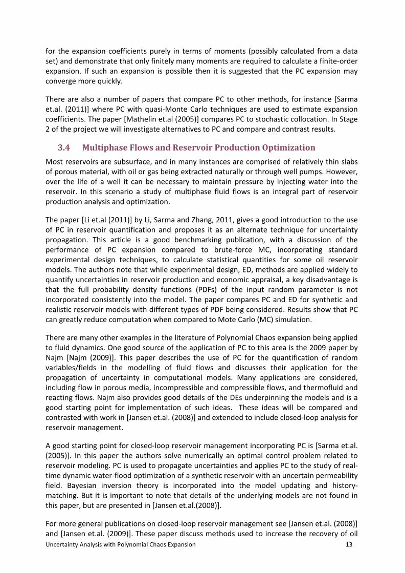
3.5 Chemical Contamination through Groundwater The transportation of contaminants through grounds water is an important component of any mineral exploration and extraction process. As in other processes uncertainty of input values governing groundwater models, necessitates the use of stochastic models for quantifying the concentration of contaminants at specific spatial locations and in different time frames. Datta and Kushwaha [Datta et.al (2011)] propose PC to quantify and propagate such uncertainty in related stochastic models.

3.6 Vortex Induced Vibrations Polynomial Chaos expansion has been used to study vortex induced vibration (VIV) in elastically mounted cylinders in a moving fluid. In most scenarios the VIV has in-line and transverse motion through the interplay of the oscillator natural frequencies and the hydrodynamic forcing terms arising from the viscous flow and quantified by Navier Stokes.

Again the natural frequencies of the oscillator are treated as random quantities, meaning that the frequency values are uncertain within certain ranges.

In our initial studies we have focussed on uncertainty propagation for two simpler problems. The first is a 2-dimensional vibration of an elastically mounted cylinder where the natural frequencies in each direction are equal and on incompressible viscous flow under uncertainty. Variants of both of these problems can then be coupled to study VIV. This work followed the papers:

[Lucor et.al. (2008)] where the authors used PC to build an accurate response surfaces for vortex-induced vibrations (VIV) of flexibly mounted cylinders with two degree-of-freedom. It provides details of stochastic DEs and uses general PC in two dimensions to solve for parameters in the associated model.

A plot of concentration of contaminants against the cumulative distribution function for a number of random input variables at t=1000 days and different distances for x.


[Xiu et.al (2002)] provides good mathematical background for the implementation of generalised PC with details of optimal polynomial bases for various input distributions presented, including the Askey scheme. PC is first applied to second-order oscillators to demonstrate convergence, and subsequently is coupled to incompressible Navier-Stokes equations. Errors are estimated and shown to compare well with similar laboratory experimental results, for the pressure distribution on the surface of a cylinder subject to vortex-induced vibrations.

3.7 Fault Tolerance and Sensitivity Testing Polynomial Chaos is seen as a highly suitable technique for testing at the tail end of probabilities and in this context for testing fault tolerance. The paper [Paffrath et.al. (2007)] uses PC to successfully approximate failure probabilities for associated DE based models. To accurately capture the tail probabilities they develop the new techniques of shifted and windowed PC. The performance of the two methods is demonstrated by a predator-prey model and a chemical reaction problem

Considerable work has been done on using PC to efficiently compute Sobol's indices, where the bulk of computation is transferred to calculating expansion coefficients. These methods have been applied successfully to finite element models, with generalized PC expansions being used to build a surrogate that allow one to compute the Sobol’s indices analytically as a post-processing of the PC coefficients. Further details can be found in [Sudret (2008)] and [Crestaux et.al. (2009)].

3.8 Stress Testing Much work has been done on combining Experimental Design techniques with PC and in particular the paper [Choi et.al 2004] provides a good discussion of the associated statistics and the implementation of regression analysis. Finite element models are analysed and in particular a model to quantify the stress occurring in a joined-wing.

3.9 Chemical Interactions Polynomial Chaos has been used broadly across the research community. One such example can be found in [Debusschere et.al. (2003)] where PC is applied to the propagation of uncertainty in a certain physical model (a coupled system of PDE). Numerical results are obtained, but are not verified. It would be good to verify these results analytically by comparing them to say Monte Carlo techniques.

3.10 Experimental Design As mentioned earlier Experimental Design techniques are an integral part of uncertainty quantification and PC. Indeed many of the PC articles are based on and compared with earlier studies using techniques, such as Monte Carlo techniques, and incorporating ED techniques (Plackett-Burman, central composite and D-optimal designs and a space filling designs) and response surface fitting techniques (kriging, splines and neural networks). For examples of such publications see [Yeten et.al. (2008)].

APPENDIX A

References

[1] L.R. Bissonnette and S.A. Orszag. Dynamical properties of truncated wiener-hermiteexpansions. Phys. Fluids, 10(12):2603–2613, 1967.

[2] K. Burrage, P. Burrage, D. Donovan, and H.B. Thompson. Populations of Models,Experimental Designs and Coverage of Parameter Space by Latin Hypercube andOrthogonal Sampling. Procedia Computer Science, 51:1762–1771, 2015.

[3] K. Burrage, P.M. Burrage, D. Donovan, T. McCourt, and H.B. Thompson. Estimateson the coverage of parameter space using populations of model. In Modelling andSimulation, IASTED, ACTA Press, 2014.

[4] R.H. Cameron andW.T. Martin. The orthogonal development of nonlinear functionalsin series of fourier-hermite functionals. Ann. Math., 48(2):385–392, 1947.

[5] Seung-Kyum Choi, Ramana V Grandhi, Robert A. Canfield, and Chris L. Pettit.Polynomial chaos expansion with latin hypecube sampling for estimating responsevariability. AIAA Journal, 42(6):1191–1198, 2004.

[6] S.K. Choi, R. V. Grandhi, and R. A. Canfield. Structural reliareliability: non-gaussianstochastic behaviour. Computers and Structures, 82(13,14):1113–1121, 2004.

[7] A.J. Chorin. Gaussian fields and random flow. J. Fluid Mech., 85:325–347, 1974.

[8] S Cremaschi, G.E. Kouba, and Subramani H.J. Characterization of confidence inmultiphase flow predictions. Energy & Fuels, 26(7):4034–4045, 2012.

[9] T. Crestaux, O. Le Maitre, and J.-M. Martinez. Polynomial chaos expansion forsensitivity analysis. Reliability Engineering and System Safety, 94(7):1161–1172,2009.

[10] S.C. Crow and G.H. Canavan. Relationship between a wiener-hermite and an energycascade. J. Fluid Mech., 41(2):387–403, 1970.

[11] D. Datta and Kushwaha.S. Uncertainty quantification using stochastic response sur-face method case study-transport of chemical contaminants through groundwater.International Journal of Energy, Information and Communication, 2(3):49–58,2011.

[12] B. Debusschere, H. Najm, Sargsyan K., and Safta C. Polynomial chaos baseduncertainty propogation intrusive and non-intrusive methods. Published atvenus.usc.edu/UQ-SummerSchool-2012/Debusschere.pdf, 2012.

[13] B. Debusschere, H. Najm, A. Matta, O. Knio, R. Ghanem, and O. Maitre. Proteinlabeling reactions in electrochemical microchannel flow: Numerical simulation anduncertainty propagation. Physics of Fluids, 15(8):2238–2250, 2003.

[14] R. Ghanem and Dham S. Stochastic finite element analysis for multiphase flow inheterogeneous porous media. Transport in Porous Media, 32:329–262, 1998.

Uncertainty Propagation with Polynomial Chaos 16

[15] Roger G. Ghanem and Pol D. Spanos. Stochastic Finte Elements: A SpectralApproach. Springer-Verlag, 1991.

[16] J.C. Helton and F.J. Davis. Latin Hypercube sampling and the propogation of uncer-tainty in analyses of complex systems. Reliability Engineering and Systems Safety,89:305–330, 2003.

[17] F. Hossain, E.N. Anagnostou, and K.-H. Lee. A non-linear and stochastic responsesurface method for bayesian estimation of uncertainty in soil moisture simulation froma land surface model. Nonlinear Processes in Geophysics, 11:427–440, 2004.

[18] Jan-Dirk Jansen, Okko H. Bosgra, and Paul M.J. Van den Hof. Model-based control ofmultiphase flow in subsurface oil reservoirs. Journal of Process Control, 18:846–855,2008.

[19] J.D. Jansen, S.D. Douma, D.R. Brouwer, P.M.J. Van den Hof, O.H. Bosgra, and A.W.Heemink. Closed-loop reservoir management. SPE International, SPE 119098, 2009.

[20] S.H. Lee and W. Chen. A comparitive study of uncertainty propogation method forblack-box-type problems. Struct Multidisc Optim, 37:239–253, 2009.

[21] O.P. LeMaitre, M.T. Reagan, H. Najm, R. Ghanem, and O.M. Knio. A stochasticprojection method for fluid flow: Ii. random process. Journal of ComputationalPhysics, 181:9–44, 2002.

[22] H. Li and D. Zhang. Probabilistic collocation method for flow in porous media:Comparisons with other stochastic methods. Water Resources Research, 43:1–13,2007.

[23] H. Li and D. Zhang. Efficient and accurate quantification of uncertainty for multimultiflow with the probabilistic collocation method. Society of Petroleum Engineers,14(4):665–679, 2009.

[24] Heng Li, Pallav Sarma, and Dongxiao Zhang. A comparative study of theprobabilistic-collocation and experimental design methods for petroleum-reservoir un-certainty quantification. SPE Journal, 16(2):429–439, 2011.

[25] D Lucor and M S Triantafyllou. Parametric study of a two degree-of-freedom cylindersubject to vortex-induced vibrations. Journal of Fluids and Structures, 24(8):1284–1293, 2008.

[26] L. Mathelin and M.Y.and Zang T.A. Hussaini. Stochastic approaches to uncertaintyquantification in cfd simulations. Numerical Algorithms, 38(1-3):209–236, 2005.

[27] M.D. McKay. Latin Hypercube sampling as a tool in uncertainty analysis of com-puter models. In J.J. Swain, D. Goldsman, R.C. Crain, and J.R. Wilson, editors,Proceedings of the 1992 Winter Simulation Conference, pages 557–564, 1992.

[28] M.D. McKay, Beckman, and Conover W.J. A comparison of three methods for select-ing values of input variables in the analysis of output for a computer code. Techno-metrics, 21:239–245, 1979.

[29] W.C. Meecham and D.T. Jeng. Use of the wiener-hermite expansion for nearly normalturbulence. J. Fluid Mech., 32:225–249, 1968.


[30] W.C. Meecham and A. Siegel. Wiener-hermite expansion in model turbulence at largereynolds numbers. Phys. Fluids, 7:1178–1190, 1964.

[31] H. Najm. Uncertainty quantification and polynomial chaos techniques in computa-tional fluid dynamics. Annual Review of Fluid Mechanics, 41:35–52, 2009.

[32] Anthony O’Hagan. Polynomial chaos: A tutorial and critique from a statistician’sperspective. 2013.

[33] S. Oladyshkin and W. Nowak. Data-driven uncertainty quantification using the ar-bitrary polynomial chaos expansion. Reliability Engineering and System Safety,106:179–190, 2012.

[34] M. Paffrath and U. Wever. Adapted polynomial chaos expansion for failure detection.Journal of Computational Physics, 226:263–281, 2007.

[35] S. Psaltis, T.W. Farrell, K. Burrage, P. Burrage, P. McCabe, T.J. Moroney, I. Turner,and S. Mazumder. Mathematical modelling of gas production and compositional shiftof a csg field 1: Local model development. Energy, 2015.

[36] M.T. Reagan, H.N. Najm, R.G. Ghanem, and O.M. Knio. Uncertainty quantificationin reaction flow simulations through non-intrusive spectral projection. Combustionand Flame, 132:545–555, 2003.

[37] P. Sarma, L.J. Durlofsky, and K. Aziz. Efficient closed-loop production optimisationunder uncertainty. Society of Petroleum Engineersprocess, SPE 94241, 2005.

[38] P. Sarma and J. Xie. Efficient and robust uncertainty quantification in reservoirsimulation with polynomial chaos expansions and non-intrusive spectral projection.SPE International, SPE 1411963, 2011.

[39] A. Siegel, T. Imamura, and W.C. Meecham. Wiener-hermite expansion in modelturbulence in the late decay stage. J. Math. Phys., 6:707–721, 1965.

[40] M. Stein. Large sample properties of simulations using Latin Hypercube sampling.Technometrics, 29(2):143–151, 1987.

[41] B. Sudret. Global sensitivity analysis using polynomial chaos expansion. ReliabilityEngineering and System Safety, (93):964–979, 2008.

[42] B. Sudret and A. Der Kiureghian. Stochastic finite element methods and reliabil-ity: A state of the art report. Technical Report UBC/SEMM-2000/08, University ofCalifornia, Berkerley, November 2000.

[43] B. Tang. Orthogonal Array-Based Latin Hypercubes. Orthogonal Array-Based LatinHypercubes, 88(424):1392–1397, 1993.

[44] E. Tixier, D. Lombardi, B. Rodriguez, and J.F. Gerbeau. Variability modelling incardiac epectrophysiology through an inverse uncertainty qantification approach. InP. Nithiarasu and E. Budyn (Eds.), editors, 4th International Conference on Com-putational and Mathematical Biomedical Engineering - CMBE2015, 2015.


[45] J.K. Vaurio. Uncertainties and quantification of common cause failure rates and proba-bilities for system analyses. Reliability Engineering and System Safety, 90:186–195,2005.

[46] W.J. Welch, R.J. Buck, J. Sacks, H.P. Wynn, T.J. Mitchell, and M.D. Morris. creening,Predicting, and Computer Experiments. Technometrics, 34:15–25, 1992.

[47] N. Wiener. The homogeneous chaos. American Journal of Mathematics, 60(4):897–936, 1938.

[48] D. Xiu and G.E. Karniadakis. Modeling uncertainty in flow simulations via generalizedpolynomial chaos. Journal of Computational Physics, 187:137–167, 2003.

[49] D Xiu, D. Lucor, C. H. Su, and G. E. Karniadakis. Stochastic modeling of flow-structure interactions using generalized polynomial chaos. Journal of Fluids Engi-neering, 124(1):51–59, 2002.

[50] D. Xiu and S.J. Sherwinb. Parametric uncertainty analysis of pulse wave propaga-tion in a model of a human arterial network. Journal of Computational Physics,226(2):1385–1407, 2007.

[51] B. Yeten, A. Castellini, B. Guyaguler, and Chen W.H. A comparison study on exper-imental design and response surface methodologies. SPE International, SPE 93347,2005.

[52] Y.K. Zhang. Stochastic Methods for Flow in Porous Media Coping with Uncer-tainties. Academic Press, 2001.


APPENDIX B

Research Notes OnUncertainty Propagation using Polynomial Chaos

Diane Donovan, Steve Lynch, Marvin Tas, Bevan Thompson and Steve Tyson

1 Uncertainty Analysis

McKay presents the following discussion about uncertainty analysis in his 1992 paper [27].An important part of model analysis is the quantification of uncertainty, particularly

the characterisation of output uncertainty due to input uncertainty; that is, quantifyingchanges in the output � given small changes in the input �. Input uncertainty mayarise because the values may be guesstimates, or they may be estimated from data, orin physical situations there might be variability from impurities. Consequently the inputis treated as a random variable with a probability distribution, and since the output iscomputed as a function of the input data, it is also treated as a random variable.Thus “the purpose of uncertainty analysis is to quantify the variability in the

output of a computer model due to variability in the values of the inputs.”[27]Ideally, knowledge of the probability distribution for � would specify the probability

distribution of � , but in practice the probability distribution of � will be estimated fromsample runs of the model. McKay’s paper [27] presents a discussion of the advantagesof using techniques based on Latin hypercube sampling, as distinct from simple randomsampling, to determine this probability distribution for the output � .

2 General discussion of Polynomial Chaos Expansion

The following general discussion about the advantages of polynomial chaos expansion(PCE) and is taken from a paper by Lucor and Triantafyllou [25]. In this paper theypropose PCE as a non-statistical method for solving differential equations that form partof a model that:

- incorporates geometry through coordinates;

- allows for uncertainty quantification of input parameters and solution outputs withina probabilistic framework.

The main advantages are that PCE allows us to:

- assign a given probability distribution to the set of input parameters;

- accurately predict the response for any set of parameters within the domain;

- develop a spectral representation for the random process in terms of orthogonal basisfunctions, thus simplifying implementation.

The positive outcomes of PCE are that this technique

- is fast and efficient;


- reduces computation cost significantly when compared to brute force methods suchas Monte-Carlo;

- propagates the effect of the chosen random distribution through the model to thenumerical solution, and so provides for sensitivity to the variability in parameters;

- provides easy access to the statistics of the random inputs, as well as, moments andprobability density functions;

- gives an expansion where the zero-index term contains the solution mean.

3 PCE, basic theory taken from O’Hagan’s tutorial [32]

For a given computer model we make the following assumptions:

- The model input is assumed to be a known random variable, �.

- The model output is also assumed to be a random variable � � ��, where � iseither a known function or � is computer generated.

Under the assumption that it may be expensive to compute � � �� or difficultto characterize it as a function of �, we make a modelling choice to recalibrate � as afunction of a more user friendly random variable � where

� � ��

So our interim goal is to approximate � such that � � ��. Note that � may not beunique. We refer to � as the germ, that may take a variety of distributions: uniformrandom variable; standard normal variable; exponential random variable.In the case of one source of uncertainty Polynomial Chaos Expansion, PCE, provides

a series expansion for the function � :

��

��

where �� are orthogonal polynomials of order �, � � �, and

��

��

converges in a meaningful way. More specifically, the expected value of the differencesquared between � and the series expansion tend to zero:

E��

��

�� as � ��

that is,��

�� converges to � in mean square. Two polynomials � and � are orthogonalif

�� E��

The key idea is to identify coefficients �� which ensure this convergence and we do thisusing a “mathematical trick” that improves accuracy and efficiency.


We begin by taking the series expansion

��

��

and multiply by �� to obtain

��

��

Now note that E�� E��

�� simplifies because �� and �� are orthogonal and��

��

�E��

�� E�� , so E�� E��

�� That is,��

��

��

��

��

��

Further using this new simplified version it is now possible to solve for �� given

��

��

��

��

��

��

Implying that

��

�� (1)

We compute for � up to � analytically, possible only for �� , otherwise we use MonteCarlo Simulation, but over a much smaller number of data points. For an alternate methodfor the computation of �� see Section 5The choice of the distribution of � is important when computing

��

��

because we would like � to be nice (especially for MCS), for example normally distributed.Once we have the coefficients ��’s and so we have � as a function of a random variable

�, we can go back to estimating the output .We note that

� ��

so let �� .The advantage here is that now is a function of � the preferred random variable and

we can repeat the process to estimate coefficients �� for � up to � in

��

��

��

��

and use��

��

��

��

It is worth remembering that PCE expands the model function using an orthogonalpolynomial series, where polynomials are chosen to match the distribution of the germ,ensuring E�� for � �� . In particular, if the germ is

- a uniformly random variable we use Legendre polynomials;

- a standard normal variable we use Hermite polynomials;

- a exponential random variable we use Laguerre polynomials.


4 Adapted PCE or failure detection

In many situations we are less interested in the full probability distribution for the outputof some model as we are in determining the probability that some user-defined ‘failure’occurs. As an example, below we consider a predator-prey model where the event that theprey population drops below a certain threshold; in other situations, a significant loss oninvestment or the destruction of some mechanical component might be classed as failures.One would hope that in any given model that failures do not occur too often, so extracare must be taken to calculate failure probabilities. Indeed, extra care must be takenwhenever one tries to estimate small probabilities numerically.In [34], Paffrath and Wever have proposed two forms of adapted PCE that hold promise

for detecting failures more effectively than the standard PCE approach described above.In this section we describe both of them and discuss the results of one application from[34].

4.1 Shifted PCE

The idea behind shifted polynomial chaos is to take expansions with respect to a proba-bility distribution whose mean coincides with the point of largest failure probability, or‘beta point’, for the model. If � is a standard normal random variable with density � anda failure is defined to be the event that �� for some function �, then the beta pointcan be determined by solving the simple optimisation problem

� ��

Taking the usual Hermite polynomials �� and applying a shift in domain �� we obtain a new basis of polynomials, which are orthogonal with respect to �� .To see this, simply compute

��

��

��

��

� ��

� ��

The belief is that the error in an expansion of � with respect to the �� should be minimisedat �, leading to better estimates on failure probabilities. Paffrath and Wever do not delveany further into theoretical aspects here, but there are some obvious questions to ask. Forexample, the total probability of failure is given by

P��

��

and we might investigate how the PCE approximation to this quantity varies as the shiftchanges. Failures are occurring over an entire region - is the beta point an optimal choice?

4.2 Windowed PCE

In windowed polynomial chaos we first determine the beta point for our model, or someapproximation to it, and then choose a neighbourhood or ‘window’ about that point


over which to approximate. If � is a random variable with probability density function��, then we may form a windowed approximation to any random variable �� of interestas follows. We first truncate and renormalise � so that it is supported in �, by setting

��

��

��

We then perform the Gram-Schmidt algorithm on the polynomial basis �� toobtain an orthogonal basis �� over �, with respect to the inner product

��

��

Finally, we compute expansion coefficients as before, but use �� to project in (1). Again,this should result in better resolution close to the beta point, however our approximationwill now contain absolutely no information about � outside of the chosen window. Anotherpossible downside is the need to re-perform Gram-Schmidt each time a new window ischosen - this is necessary since the truncated distribution �� will almost never have astandard form, and so the standard polynomial bases become unavailable.

5 Alternate method for calculating coefficients

Equation 1 describes how to determine the coefficients �� in the PCE using analytical ornumerical techniques. Choi, Grandhi, Canfield and Pettit [5] describe how these coeffi-cients can be estimated using regression analysis based on Latin hypercube sampling.A Latin Hypercube Sample of dimension �, with underlying set � �� , is a

set of �-tuples chosen from � such that each component takes the set of values .More precisely, a Latin Hypercube Sample, LHS, is a set � � �� such that

��

for � ��

LHSs over a �-dimensional parameter space are easy to generate and can be representedas an � array � � �� , (� � � , � � � � �), where each row corresponds to a�-tuple. For instance:

1) For each variable ��, � � � � �, divide the range of that variable into non-overlapping intervals ��, � � � on the basis of equal probability.

2) For each column � generate a random permutation �� on the set �� . For� � � , if �� , then randomly select (with respect to its probability densityfor the given variable) one value �� and set �� .

3) Repeat Step 2 for all � � �� until we have filled the � array.

Now this LHS can be combined with PCEs to build an approximation for the responsemodel for the uncertain parameters. Choi et.al. begin with the following insightful discus-sion for a simple model for approximating the non-linear relationships. This model takesthe form

� ��


In this model, �� and �� are the mean, linear, quadratic, and cubic effects of theresponses, respectively, and most of the time model uses polynomials

��

However, since these functions are not orthogonal, the computation can be excessive forsay large positive values for � and for large negative values for � the cubic power takes largenegative values while the quadratic term take large positive values. Thus small changes in� �� could result in large changes in the coefficients �� and the associated least-squares problem may be ill conditioned. The alternative is to use orthogonal polyomialsand implement PCE.Choi et.al. provide a general discussion of PCE, where in their notation they write the

PCE as

��

�

��

where � is a random character used in the estimation of the variables, �� are the coefficientsof interest and �� are the orthogonal polynomials. They comment that if a solutionis known then the coefficients �� can be calculated as

��

��

where often MCS is used to evaluate the expected values. However Choi et.al. proposean alternative to MCS based on LHS and illustrate their method on a simple example, aspresented in the next subsection.So in summary the Choi et.al. procedure, [5], is as follows.

1) Select experimental designs using LHS.

2) Simulate system response at each design point.

3) Construct approximate model using PCE.

4) Conduct ANOVA and residual analysis.

6 Applications and Examples

6.1 A simple example

Choi, Grandhi and Canfield [5] studied the simple model is � ��, where � is a normalrandom variable which has a mean of 2, unit standard deviation and is approximatedby a second-order polynomial model:

� � ��

where is a standard normal distribution �� . Their choice of orthogonal polynomialsis:

��


and where the random variable � is transformed as

� � ��

Then the unknown coefficients are found by first using LHS to identify points in theparameter space, then �� are determined using regression analysis based on theselected points.Choi et.al. repeat this process for a third-order polynomial model where coefficients

�� are calculated and it is found that �� is insignificant. Using arguments sup-ported by statistics given in an ANOVA table, they deduce that the third-order polynomialis sufficient for the fitting.They go on to comment that in this simple example the error can be determined by

plotting the response and comparing it to the MacLaurin polynomial. In other, more indepth, examples it is possible to check the error using residual analysis.Choi et.al. then go on to apply the same procedure to a �-dimensional model � �

��, and in the later stages of the paper illustrate with a practical example analysingbuckling in a joined-wing model.

6.2 PCE applied to Spring and Harmonic Motion

To demonstrate the applicability of PCE to models built around differential equations, weconsider the equation of motion for a unit mass on a spring,

��

Here � stands for the displacement of the mass and � for the spring constant. Even ifwe introduce some randomness by taking � � �� to be a strictly positive, uniformlydistributed random variable, the resulting equation

�� (2)

can be solved analytically. For illustration however, let us expand � and � as truncatedseries of Legendre polynomials:

��

��

��

��

��

Notice that the coefficients of � are now time dependent, while the polynomial basisremains fixed. Substituting these expansions back into the DE then yields

��

��

��

��

��

��

��

��

��

� ��

��

��

We now make use of the orthogonality of our polynomial basis once more. The projectionof the left-hand-side onto any � simplifies to

� ��

��

��

�

��

��


while on the right we obtain��

��

��

��

��

��

��

��

so we see that

��

��

��

��

�� (3)

Hence the problem of calculating the coefficients �� reduces to solving the deterministicsystem of coupled ODE’s (3). The hope is that solving this system for a surrogate andusing that to run simulations will be more efficient than repeatedly solving (2), as a crudeMonte-Carlo approach would require. It is worth noting that each of the values �� can be found analytically. Indeed, many of them vanish.

6.3 A predator-prey model

Paffrath and Wever achieved some success at predicting failure probabilities in a simplepredator-prey model, the Lotka-Volterra system:

��

��

Here the coupling constants �, and � are all taken to be positive and � and respectivelymeasure the time-dependent sizes of prey and predator populations in an ecosystem. Theauthors introduce randomness by allowing �� to be normally distributed with mean 1and standard deviation 0.01, and define a failure to be the event that �� . Theythen fix a set of initial conditions and run a large number of Monte-Carlo simulations toobtain a near-exact estimate of the failure probability over time. This was then comparedto estimates obtained by expanding �, and � in third-order Hermite expansions withrespect to a standard normal (CH), a normal with shift � � (SH), and a windowednormal (WH) with � �� . The results are summarised in Figure ??.Clearly the accuracy of the three different approximations is highly dependent on time,

but each performs well at least on some interval. This raises a number of questionsregarding optimal choices of windows and shifts, and how these choices depend on theevolution of a system, but demonstrates the potential of both techniques.

6.4 PCE applied to a vortex induced vibration scenario

In this section, we are working towards using PCE to study vortex induced vibration (VIV)in elastically mounted cylinders in a moving fluid. The VIV has in-line and transversemotion through the interplay of the oscillator natural frequencies and the hydrodynamicforcing terms arising from the viscous flow and quantified by Navier Stokes. Again thenatural frequencies of the oscillator are treated as random quantities, meaning that thefrequency values are uncertain within certain ranges.We begin by focussing on uncertainty propagation for two much simpler problems.

The first is a 2-dimensional vibration of an elastically mounted cylinder where the naturalfrequencies in each direction are equal. The focus is on incompressible viscous flow underuncertainty. Variants of both of these problems can then be coupled to study VIV.


6.4.1 Mathematics for UQ using PCE to model oscillating cylinders

In the first example we use PCE to solve differential equations that model an elasticallymounted cylinder with natural frequencies of oscillation which are random variables andsubject to random forces.Let the position of the centre of the cylinder be �� where

��

��

��

� ��

�� and �� represent the natural frequencies of the oscillatoralong the �� and �� directions, respectively. Here the uncertainty is represented by thedependency on �.For VIV the hydrodynamic forcing �� acts as a coupling between these equations

whose solutions are computed iteratively.We may use a parametric representation of the second order stochastic process:

X��

with X�� varying randomly over time � as

��

��

��

� ��

��

��

In this PCE

� ��, � � N, are zero-mean random vectors (uncertain sets of parameters)dependent on a random event � chosen from a random event space ;

� �� and �� are coefficients of interest;

� �� are orthogonal polynomials over the domain ��.

We use Legendre polynomials as are uniformly distributed.For now we simplify the above presentation and use an approach suggested by Xiu,

Lucor, Su and Karniadakis [49].So starting with

�� (4)�� (5)

we relabel as X � x, �� and �� Then let �x � y and theequation can be rewritten as

x

�� y�

y

�� y � ��x � f��

Here x� y� f are two dimensional and �� and �� are correlated random variables.


Then we use PCE to approximate � and � as follows

� ��

��

��

� ��

��

� ��

��

where �� are coefficients of the PCE of �� respectively. Note that we

have truncated to a finite sum. This is then applied in the differential equations

��

��

��

��

��

��

��

��

��

��

��

��

��

��

��

��

��

��

��

��

��

��

��

��

To illustrate the solution technique we only take one of the Equations 4 and 5.There is some work to be done using a Galerkin projection of the above equation

onto each polynomial basis �� to ensure the error is orthogonal to the functional spacespanned by the finite-dimensional basis ��. However with a bit of work the abovesimplifies to

��

�� (6)

��

��

�

��

��

��

��

��

��

��

��

��

��

�� (7)

where �� and �� ; here �� E��This gives a set of �� coupled ODEs with the terms �� and ��

� � beingevaluated analytically from the definition of ��.Here we can use some standard tricks to simplify the calculations.

� If we assume that the natural frequency of the oscillator is uniformly distributed(a natural assumption in this setting) then we can use Legendre polynomials �� so��

�� where � is Kronecker delta � � if � � � and � � otherwise.

� Moreover �� so after scaling

��

�

��

��

��

where we have rescaled the mean zero uniform random variable � to have the PDFequal to �� on �� .

� Now �� is a polynomial of degree at most � � so Gaussian Quadraturecould be used to compute the ��

��, �� and �� although analytic formula are notdifficult to compute in this case.

Now (6) and (7) are a coupled system of � � �� ODEs which can be solved accu-rately and efficiently through code developed by Shampine that is incorporated in severalpackages including Matlab.


6.4.2 Uncertainty propagation using PCE applied to Navier Stokes

We are now in a position to consider a more complicate scenario.Let the 2-dimensional velocity field be given by u�� We consider incompressible flow so u satisfies the following Navier Stokes equation

� � u � �� (8)�u

�� u � ��u � ��

��u� (9)

Here �� is the Reynolds number and � is the pressure.Now expand u and � � to order � ; that is, set

u�x� ��

��

u��x� ��

��x� ��

��

��x� ��

The Navier Stokes equations become

��

��

� � ui� � ��

��

��

�u�

��

��

��

��

��

�u� � ��u��

��

��

��

��

��u��

Similarly to the ODE case projecting onto the random space spanned by ��and

taking inner products with each of � we obtain

� � uk � ��

�u�

��

��

��

��

��

��

��

�u� � ��u�� u��

Thus we have a set of � � equations that are Navier Stokes like. We can changecoordinates setting x � x� � ��x� �� where now the �� and �� variables are theoriginal variables. Thus linking an ODE variant of Equations 6 and 7 with the PDE, forthe case of one cylinder.The combined system of PDEs and ODEs have to be solved together. This is done

iteratively one time step at a time.Returning to the paper by Lucor and Traintafyllou [25] where they choose the time

step to be 1/5 of the natural frequency of the oscillator. They consider two cases: onewhere the natural frequency in the inline direction is the same as in the transverse direc-tion and another where these are different; one can take � �

��

�� where the ��

are independently and identically distributed (iid) uniform random variables; again theseshould be independent of the other random variables.We need boundary conditions, so we consider upstream a constant velocity U which we

assume is subject to uniformly distributed noise so U � �� i� here i is a unit vectorin the inline � direction while � is a uniformly distributed random variable with mean 0and variance � In the new coordinates the RHS of (8) acquires the term A�� and the cylinder occupies x � 0.


Of course � and � are independent random variables where � is the uniformly dis-tributed uncertainty in the natural frequency of the elastically supported cylindrical bluffbody.The fluid forces on the cylinder are computed by

F ��

��n��u��u� � � n��

where n is the outward normal on the cylinder, �� is arc length around the curved surfaceof the cylinder.Also � is the diameter of the cylinder and

��

�

��

�

and ��

�

��

�

7 Weather derivatives

A very brief summary of Pricing weather derivatives, PhD thesis by B Petschel.Electricity producer’s profit depends directly on electricity demand and data shows

that power usage depends significantly on temperature through air-conditioning (quitemarkedly in Australia since around 2000).Basic information

- Weather (temp.) derivatives are financial contracts with payoffs depending onheating degree days (HDD) and cooling degree days (CDD).

- CDD measures how much the daily average temperature exceeds 65 deg F (temper-ature in US Govt buildings).

- Temperature model cannot be based on normal variables since this leads to toomany outliers in the fit.

- The Solution is to add a jump term to the temperature model.

- Temperature Model is a stochastic differential equation with jumps; the temper-ature (solution) is a random variable.

Temp � Av. Temp. � random, drifting & jumping, process

used to approximate the cooling degrees days; the solution is integrated over timeapproximating average temperature, which is a random variable.

The result is a model that fits Brisbane temperature data fairly well.

However we now have a problem because adding a jump means that temperature(solution) no longer has a nice formula.Ben’s solution is to get a formula for the moment generating function, which can be

expressed in terms of its moments (mean, variance, kurtosis etc). Hermite polynomials(functions) are used to approximate the generating function and moments can be obtainedas a by product of the procedure. We can price CDD contracts using moments.


7.1 PCE and Ben’s problem

Both problems essentially reduce to

��

��

��


Uncertainty Modelling with Polynomial Chaos Expansion 1_Final... · Uncertainty Analysis with...

Documents

Transcript of Uncertainty Modelling with Polynomial Chaos Expansion 1_Final... · Uncertainty Analysis with...