Generalized polynomial chaos and stochastic collocation … · 2019-01-14 · Generalized...

Generalized polynomial chaos and stochastic collocation methods

for uncertainty quantification in aerodynamics

J. Peter , Eric Savin (1)

(1)ONERA DAAA - DTIS

November 2018

J. Peter et al. (ONERA DAAA) November 2018 1 / 101

Outline

1 Introduction. Need for Uncertainty Quantification

2 Probability basics, Monte-Carlo, surrogate-based Monte-Carlo

3 Non-intrusive polynomial methods for 1D / tensorial nD propagation

4 Introduction to Smolyak’s sparse quadratures

5 Examples of application

6 Conclusions


Introduction. Need for Uncertainty Quantification

Outline






6 Conclusions



Need for (UQ)Example I : drag evaluation

Deterministic drag of airplane in cruise

Total drag Cd at cruise nominal Mach number (M=0.82) Cd(0.82)a/c shape satisfying constraints on lift, pitching moment, rolling moment...

Actually cruise flight Mach number varies

Waiting for landing slotSpeeding up to cope with pilot maximum flight time

→ Variable Mach number described by D(M)

Robust calculation of airplane cruise drag

Compute∫Cd(M)D(M)dM, instead of Cd(0.82)



Need for (UQ)Example II : fan design

Fan operational conditions subject to changes in wind conditions

Manufacturing subject to tolerances

Robust design accounts forvariability of external parameterstolerances for internal parameters

Figure: Robust design (from cenaero.be)



Need for (UQ)Example III : validation process

Unkown data in experiment

Upwind Mach number (equivalent to far-field Mach number in free-stream)not fully controled in wind tunnels dM = 0.001

Unknown physical constant needed in numerical model

Wall roughness constant (milled, brazed, eroded surface...)

Discrepancy in a computational/experimental validation process !

Compute the mean and standard deviation of the output(s) of interest due tothe uncertain inputs



(UQ) inputs and outputsDefinition of uncertain inputs

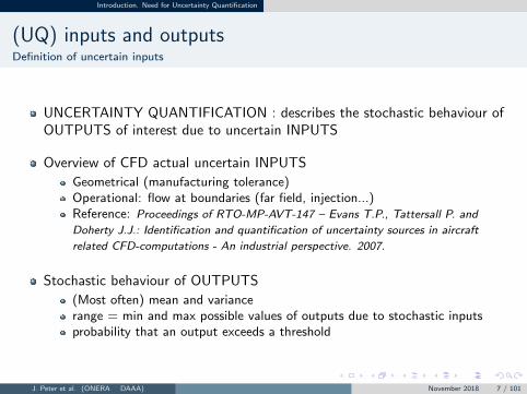
UNCERTAINTY QUANTIFICATION : describes the stochastic behaviour ofOUTPUTS of interest due to uncertain INPUTS

Overview of CFD actual uncertain INPUTS

Geometrical (manufacturing tolerance)Operational: flow at boundaries (far field, injection...)Reference: Proceedings of RTO-MP-AVT-147 – Evans T.P., Tattersall P. and

Doherty J.J.: Identification and quantification of uncertainty sources in aircraft

related CFD-computations - An industrial perspective. 2007.

Stochastic behaviour of OUTPUTS

(Most often) mean and variancerange = min and max possible values of outputs due to stochastic inputsprobability that an output exceeds a threshold



Three issues with (UQ)1 terminology

Lack of agreement on the definition of “error”, “uncertainty”...

AIAA Guide G-077-1998 Uncertainty is a potential deficiency in any phase areactivity of the modeling process that is due to the lack of knowledge. Error isa recognizable deficiency in any phase or activity of the modelling processthat is not due to the lack of knowledge

ASME Guide V& V 20 (in its simpler version adopted for the LisbonWorkshops on CFD uncertainty) The validation comparison error is definedas the difference between the simulation value and the experimental datavalue. It is split in numerical, model, input and data errors (assumed to beindependant). Numerical (resp. input, model, data) uncertainty is a bound ofthe absolute value of numerical (resp. input, model, data) error



Three issues with (UQ)2 (UQ) validation and verification

(UQ) CFD-based exercise leads to standard deviation of some outputs

Compare this standard deviation to the discretization error

Richardson method, GCI...Pierce et al. Venditti et al. adjoint based formulas for functional outputs

Compare this standard deviation to the modeling error

Run several (RANS) modelsRun better models than (RANS)

Numerical (UQ) investigation only makes sense if standard deviation due touncertain inputs not much smaller than modelling or discretization error



Three issues with (UQ)3 lack of shared well-defined problems ?

Quite difficult to get information from industry in order to define relevant(UQ) exercises

Quite difficult to understand when industry uses (UQ) and when industryuses multi-point analysis / optimization to deal with parameter variations

Do not only common problems with in-house CFD and chosen (UQ) method.Also share

mathematical test cases with specific complexitymathematical test cases derived from industrial cases (using surrogates)

or it is difficult/impossible to split the influence of discrepancies in CFDmethods and the one in (UQ) methods



Slides and lecture notes

ONERA involved in EU projects, RTO project on (UQ)

Provide accessible information for non-experts

Examples, illustrations, explicit 2D formulas...

Slides and lecture notes


Probability basics, Monte-Carlo, surrogate-based Monte-Carlo

Outline






6 Conclusions



Basics of probability (1)

A classical introduction to probability basics involves

event (one dice value, one Mach number value)

a sample space Ω (all six dice values, interval of Mach number values)

set of events space A (σ-algebra) set of subsets of Ω, stable by union,intersection, including null set ∅ and Ω

a probability function P on A such that P(Ω) = 1,P(∅) = 0, plus naturalproperties for complementary parts and union of disjoint parts

OUT random variables X depending on the event ξ (like CDp or CLp of an airfoildepending on the far-field Mach number through Navier-Stokes equations)




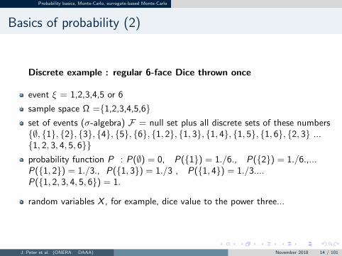
Discrete example : regular 6-face Dice thrown once

event ξ = 1,2,3,4,5 or 6

sample space Ω =1,2,3,4,5,6set of events (σ-algebra) F = null set plus all discrete sets of these numbers∅, 1, 2, 3, 4, 5, 6, 1, 2, 1, 3, 1, 4, 1, 5, 1, 6, 2, 3 ...1, 2, 3, 4, 5, 6probability function P : P(∅) = 0, P(1) = 1./6., P(2) = 1./6.,...P(1, 2) = 1./3., P(1, 3) = 1./3 , P(1, 4) = 1./3....P(1, 2, 3, 4, 5, 6) = 1.

random variables X , for example, dice value to the power three...




Continuous example : Far-field Mach number in [0.81,0.85]

event ξ = a Mach number value in [0.81,0.85]

sample space Ω = [0.81,0.85]

set of events (σ-algebra) F = all subparts of [0.81,0.85]

probability function P. Probability of (union of) intervals I ∈ Fto be defined from a probability density function D, integrating D over I .

Example: Dφ(φ) =35

32(1.− φ2)3 φ ∈ [−1, 1] φ = (ξ − 0.83)/0.02

Dξ(ξ) =1

0.02Dφ(φ) =

1

0.02

35

32(1.− (

ξ − 0.83

0.02)2)3

possible random variables X = lift, drag, pitching moment of a wing... withvariable Mach number M∞(“event“ ξ) in the farfield



Basics of probability (4)Example of probability density functions

Set of probability density functions of β−distributions on [0,+1] with the α− 1β − 1 convention for exponants

Dα,β(x) =xα−1(1− x)β−1∫ 1

0tα−1(1− t)β−1dt

x ∈ [0, 1]



Need for (UQ)Intrusive vs non-intrusive methods

Non-intrusive methods. No change in the analysis code

Post-processing of deterministic simulations

Intrusive methods. Changes in the analysis code

Stochastic expansion of state/primitive variablesGalerkin projections. Larger set of equations

Probably not feasible for large industrial codes



Monte-Carlo – 1

Monte-Carlo mimics the law of the event in a series of calculations

Reference method for all uncertainty propagation methods

Generation of a sampling (ξ1, ξ2..., ξp..., ξN ...) of the p.d.f D(ξ)

Computation of corresponding flow fields W (ξp), p ∈ [1,N]

Computation of functional outputs J (ξp) = J(W (ξp),X (ξp))Discrete estimation of mean and variance:

E(J ) =

∫J (ξ)D(ξ)dξ ' JN =

1

N

p=N∑p=1

J (ξp)

σ2J = E((J − E(J ))2) =

∫(J (ξ)− E(J ))2D(ξ)dξ ' σ2

JN=

1

N − 1

p=N∑p=1

(J (ξp)− JN)2

Need to quantify accuracy of estimation



Monte-Carlo – 2Accuracy of mean

Scalar case, variance σJ is known, N sampling size,√N JN−E(J )

σJ N (0, 1)

(Normal distribution)

Probability density function (p.d.f.) of N (0, 1)- DN (x) = 1√2Π

e−x2

2

Symmetric cumulative distribution function - ΦN (x) = 1√2Π

∫ x

−x e− t2

2 dt

With ε confidence : E (J ) ∈ [JN − uεσJ√N, JN + uε

σJ√N

] ε = 1√2Π

∫ uε

−uεe−

t2

2 dt

ε 0.5 0.9 0.95 0.99uε 0.674 1.645 1.960 2.576

With 99% confidence :

E (J ) ∈ [JN − 2.576σJ√N, JN + 2.576

σJ√N

] (0.99 =1√2Π

∫ 2.576

−2.576

e−t2

2 dt)




Scalar case, variance σJ is unknown, N sampling size,√N JN−E(J )

σJN S(N − 1) – Student distribution

With ε confidence :

E (J ) ∈ [JN − uε(N−1)

σJN√N, JN + uε(N−1)

σJN√N

]

uεN as function of ε and N found in tables. uεN decreases with N increasing

Student distribution converges to Normal distribution for large N

Tables for uεN−1

ε N 1 2 20 30 ∞0.95 12.71 4.303 2.086 2.042 1.9600.99 63.66 9.925 2.845 2.750 2.576

Figure: Value of uε(N−1) for Student distribution S(N − 1) N ≥ 2




Scalar case: variance σJ is unknown, N sampling size√N JN−E(J )

σJN S(N − 1) – Student distribution

Student distribution S(N) probability density function:

DS(N)(x) =Γ(N+1

2 )

Γ(N2 )√NΠ

(1 +x2

N)−

N+12

(Γ(u) =

∫ +∞

0

tu−1e−tdt

)

With ε confidence (ε ∈]0, 1.[):

E (J ) ∈ [JN − uε(N−1)

σJN√N, JN + uε(N−1)

σJN√N

] ε =

∫ uεN−1

−uεN−1

DS(N−1)(t)dt



Monte-Carlo – 5Accuracy of estimation: variance (1) (skpd)

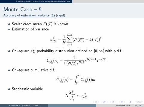
Scalar case: mean E (J ) is known

Estimation of variance

σ2JN

=1

N

i=N∑i=1

(J (ξp)− E (J ))2

Chi-square χ2N probability distribution defined on [0,∞[ with p.d.f. :

Dχ2N

(x) =1

Γ(N/2)2N/2xN/2−1e−x/2

Chi-square cumulative d.f. :

Φχ2N

(x) =

∫ x

0

Dχ2N

(t)dt

Stochastic variable

NS2JN

σ2J χ2

N



Monte-Carlo – 6Chi-square probabilistic density functions Dχ2

Nand cumulative density functions Φχ2

N(skpd)



Monte-Carlo – 7Accuracy of variance (2) (skpd)

Scalar case: mean E (J ) is known - Nσ2JNσ2J χ2

N

With ε = 1− α confidence :

Φ−1χ2N

(α

2) ≤ N

σ2JN

σ2J≤ Φ−1

χ2N

(1.− α

2)

With ε = 1− α confidence :

σ2J ∈ [N

σ2JN

Φ−1χ2N

(1− α2 ),N

σ2JN

Φ−1χ2N

(α2 )]

x N 2 20 300.005 10.597 39.997 53.6720.995 0.0100 7.434 13.787

Figure: Value of Φ−1

χ2N

(x)




Application. With 99% confidence, depending on N number of samples

N = 2⇒ σ2J ∈ [0.189 S2

J2, 200 S2

J2]

N = 20⇒ σ2J ∈ [0.500 S2

J20, 2.69 S2

J20]

N = 30⇒ σ2J ∈ [0.559 S2

J30, 2.18 S2

J30]

N = 100⇒ σ2J ∈ [0.713 S2

J100, 1.49 S2

J100]

Convergence speed of bounds towards 1.

The cumulative distribution of the Chi-Square law ΦN(x) can be expressed as

Φχ2N

(x) = 1Γ(N/2)

∫ x/2

0

tN/2e−tdt =γ(N/2, x/2)

Γ(N/2)(γ lower incomplete Γ

function)

Check properties of (the inverse of) Φχ2N

Check convergence speed of N/Φ−1χ2N

(1− α2 ) and N/Φ−1

χ2N

(α2 )




Scalar case: mean E (J ) is unknown - Stochastic variable

(N − 1)σ2JNσ2J χ2

N−1

With ε = (1− α) confidence :

σ2J ∈ [(N − 1)

σ2JN

Φ−1χ2N−1

(1− α2 ), (N − 1)

σ2JN

Φ−1χ2N−1

(α2 )]

x N 3 4 20 300.005 10.597 12.838 38.582 52.3360.995 0.0100 0.0717 6.844 13.121

Figure: Value of Φ−1

χ2N−1

(x)



Monte-Carlo – 10Cost issue. Regularity of output.

Typical realistic estimation of accuracy of mean estimated by Monte-Carlo is :

With a N point sampling, with 99% confidence :

E (J ) ∈ [JN − u0.99,(N−1)σJN√N, JN + u0.99,(N−1)

σJN√N

]

with u0.99,1 = 63.66, u0.99,2 = 9.925, u0.99,3 = 5.841, u0.99,9 = 3.250,u0.99,19 = 2.861, u0.99,19 = 2.756,... decreasing with the number of samples,N, towards limiting value 2.576.

Convergence speed of Monte-Carlo for mean value estimation is 1√N

Increasing precision of Monte-Carlo estimation by a factor of 10 requiresmultiplying the number of evaluations by a factor of 100

Extremely expensive if one evaluation requires numerical solution ofEuler or (RANS) equations



Monte-Carlo – 11Cost issue. Regularity of outputs

Convergence speed of Monte-Carlo for mean value estimation is 1√N

Extremely expensive if one evaluation requires numerical solution ofEuler or (RANS) equations

Besides ouputs of CFD calculations are often very regular functions of theparameters of interest

Take advantage of the regularity of (random) output variables seen asfunction of (stochastic/events) inputs variables

Derive a surrogate of the output variables as function of the input variablesusing specific stochastic surrogates → next section

Derive a surrogate of the output variables as function of the input variablesusing general surrogates → end of this section section

Calculate mean, variance, kurtosis, range, risk... for the surrogate



Meta-model based Monte-Carlo

Figure: Monte-Carlo method with meta-modelsJ. Peter et al. (ONERA DAAA) November 2018 29 / 101


Meta-models

Restriction: approximation of a function of interest. What kind of surrogatecan be used ?

1 Classical metamodels: Kriging, Radial Basis Function, Support VectorRegression. (used regularly at ONERA 1)

2 Other meta-models of specific interest for UQ: generalized polynomial Chaos(gPC), Stochastic Colllocation (SC)

3 Other model of specific interest for large dimensions: adjoint based linear orquadratic Taylor expansion

Influence of meta-model accuracy on mean and variance accuracy ?

1Modeles de substitution pour l’optimisation globale de forme en arodynamique et mthodelocale d’optimisation sans paramtrisation. Manuel Bompard. PhD Thesis. December 2011



Application of metamodel-based Monte-Carlo

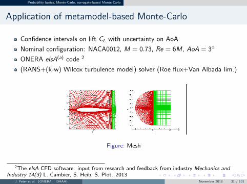
Confidence intervals on lift CL with uncertainty on AoA

Nominal configuration: NACA0012, M = 0.73, Re = 6M, AoA = 3

ONERA elsA(a) code 2

(RANS+(k-w) Wilcox turbulence model) solver (Roe flux+Van Albada lim.)

Figure: Mesh

2The elsA CFD software: input from research and feedback from industry Mechanics andIndustry 14(3) L. Cambier, S. Heib, S. Plot. 2013



Distribution of uncertainty

Beta distribution (parameters (3.,3.))over [-1,1]

Db(ξ) =15

16(1− ξ)2(1 + ξ)2

p.d.f of angle of attack AoA over [2.9,3.1]

Da(α) = 10Db(10.(α− 3.))

Figure: Beta distribution of AoA



Monte-Carlo method for CL mean

0.484

0.486

0.488

0.49

0.492

0.494

0.496

0.498

1 10 100 1000

Estimated mean value90 percent95 percent99 percent

Best MC with MM value

Figure: Mean of CL coefficient and confidence interval



Monte-Carlo method for CL variance

0

2e-05

4e-05

6e-05

8e-05

0.0001

0.00012

0.00014

0.00016

0.00018

0.0002

1 10 100 1000

Estimated variance value90 percent95 percent99 percent


Figure: Variance of CL coefficient and confidence interval



Metamodel based Monte-Carlo: learning sample

Use learning sample based on roots of Tchebyshev polynomials

2.90 2.92 2.94 2.96 2.98 3.00 3.02 3.04 3.06 3.08 3.10−1

0

1

Figure: Tchebychev distribution (11 points)



Metamodel-based Monte-Carlo: reconstruction of CL

Figure: CL



Metamodel-based Monte-Carlo for CL meancalling metamodel instead of CFD code

0.484

0.486

0.488

0.49

0.492

0.494

0.496

0.498

1 10 100 1000 10000 100000 1e+06 1e+07

Estimated mean value90 percent95 percent99 percent


Figure: Mean of CL coefficient and confidence interval



Metamodel-based Monte-Carlo for CL variancecalling metamodel instead of CFD code

0

2e-05

4e-05

6e-05

8e-05

0.0001

0.00012

0.00014

0.00016

0.00018

0.0002

1 10 100 1000 10000 100000 1e+06 1e+07

Estimated variance value90 percent95 percent99 percent


Figure: Variance of CL coefficient and confidence interval


Non-intrusive polynomial methods for 1D / tensorial nD propagation

Outline






6 Conclusions



Two polynomial methods for (UQ). 1D and nD tensorial

Stochastic specific polynomial surrogates

For all non-intrusive methods

Presentation for one uncertain parameter ξ, probability density function D(ξ)

Extention to a vector of two uncertain parameters ξ = (ξ1, ξ2) under therestriction that

D(ξ) = D1(ξ1)× D2(ξ2)

and no sparsity is sought for = extension of N-point evaluation method in 1Duses N2 evaluations in dimension 2

Extrapolation to d-D to discuss complexity and cost

Generalized polynomial chaos method

Stochastic collocation method



Generalized polynomial chaos Method (gPC) – 1

Polynomial expansion of the quantity of interest, scalar output or vector

F (ξ) ' gF (ξ) =l=M∑l=0

ClPl (ξ)

Coefficients of the expansion computable by different methods (quadrature, collocation)

Polynomial basis orthogonal for the dot product defined by the p.d.f. D(ξ)

< Pl ,Pm >=

∫Pl (ξ)Pm(ξ)D(ξ)dξ = δlm

Straightforward calculation of mean and variance of the polynomial expansion (thatapproximates the quantity of interest)

Orthogonal polynomials – Abramowitz and Stegun: Handbook of Mathematical functions.(1972). Chapter 22

Spectral expansions – J. P. Boyd: Chebyshef and Fourier spectral methods (2001)



Generalized polynomial chaos Method (gPC) – 2Families of orthogonal polynomials

Normal distribution Dn(ξ) = 1√2Π

e−ξ2

2 on R → Hermitte polynomials

Gamma distribution Dg (ξ) = exp(−ξ) on R+ → Laguerre polynomials

Uniform distribution Du(ξ) = 0.5 on [−1, 1]→ Legendre polynomials

Chebyshev distribution Dcf (ξ) = 1/Π/√

1− ξ2 on [−1, 1]→ Chebyshev (first-kind)polynomials

Chebyshev distribution Dcs(ξ) =√

1− ξ2 on [−1, 1]→ Chebyshev (second-kind)polynomials

Beta distribution Dβ(ξ) = (1− ξ)α(1 + ξ)β/∫ 1−1(1− u)α(1 + u)βdu

α > −1. , β > −1. on [−1,+1] → Jacobi polynomials (incl. Chebyshev polynomials)

Non-usual probabilistic density functions, Dl (ξ) computed by Gram-Schmidtorthogonalisation process.




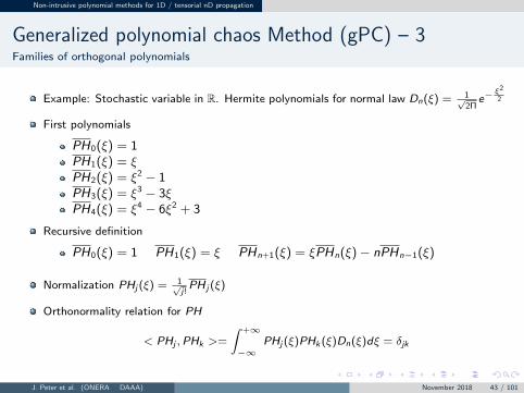
Example: Stochastic variable in R. Hermite polynomials for normal law Dn(ξ) = 1√2Π

e−ξ2

2

First polynomials

PH0(ξ) = 1PH1(ξ) = ξPH2(ξ) = ξ2 − 1PH3(ξ) = ξ3 − 3ξPH4(ξ) = ξ4 − 6ξ2 + 3

Recursive definition

PH0(ξ) = 1 PH1(ξ) = ξ PHn+1(ξ) = ξPHn(ξ)− nPHn−1(ξ)

Normalization PHj (ξ) = 1√j!PH j (ξ)

Orthonormality relation for PH

< PHj ,PHk >=

∫ +∞

−∞PHj (ξ)PHk (ξ)Dn(ξ)dξ = δjk




Example: Stochastic variable in [-1,1]. First-kind Chebyshef polynomials for probabilitydensity function Dcf (ξ) = 1

Π1√

1−ξ2

Family of orthonormal polynomials for < f , g >=∫ 1−1 f (t)g(t)Dcf (t)dt

T 0(ξ) = 1T 1(ξ) = ξT 2(ξ) = 2ξ2 − 1T 3(ξ) = 4ξ3 − 3ξ

Recursive definition

T 0(ξ) = 1 T 1(ξ) = ξ T n+1(ξ) = 2ξT n(ξ)− T n−1(ξ)

Normalization T0 = T 0 T1 =√

2 T 1... Tn =√

2 T n (n ≥ 1)

Orthonormality of the Tj ,

< Tj ,Tk >=∫ 1−1 Tj (ξ)Tk (ξ)Dcf (ξ)dξ = δjk

Specific property T n(cos(θ)) = cos(nθ) (hence ||T n||∞ ≤ 1.)



Generalized polynomial chaos Method (gPC) – 5Polynomial expansion

Expansion of a functional output depending on stochastic variable ξ

F (ξ) ' gF (ξ) =l=M∑l=0

ClPl (ξ)

Expansion of a field on part of the mesh depending on stochastic variable ξ (i is a genericindex for a part of the mesh nodes like wall nodes)

W (i , ξ) ' gW (i , ξ) =l=M∑l=0

Cl (i)Pl (ξ)

Accuracy of ideal gW depending on degree and regularity. Theory of spectral expansions

Stochastic post-processing for gW (gF ) instead of W (F )

Straighforward calculation of gW (gF ) mean and variance



Generalized polynomial chaos Method (gPC) – 6Coefficients computation (1/4) - Gaussian quadrature

Expansion of part of flow field depending on stochastic variable ξ and generic mesh index i

W (i , ξ) ' gW (i , ξ) =l=M∑l=0

Cl (i)Pl (ξ)

From orthonormality property Cl (i) =< gW (i),Pl > Under regularity assumptionsCl (i) =<W (i),Pl >

Proof Assume D is defined on an interval of R and bounded. Assume uniform convergence of spectralexpansion over its domain of definition

W (i, ξ) =l=∞∑l=0

Cl (i)Pl (ξ)

Multiply by Pn(ξ)D(ξ)

W (i, ξ)Pn(ξ)D(ξ) =l=∞∑l=0

Cl (i)Pl (ξ)Pn(ξ)D(ξ)

Integrating over domain of definition of D(ξ) yields Cn(i) =< W (i),Pn >



Generalized polynomial chaos Method (gPC) – 7Coefficients computation (2/4) - Gaussian quadrature


gW (i , ξ) =l=M∑l=0

Cl (i)Pl (ξ) Cl (i) =< gW (i),Pl >

Gaussian quadrature for

Cl (i) =<W ,Pl >=

∫W (i , ξ)Pl (ξ)D(ξ)dξ

Computation by Gaussian quadrature associated to p.d.f D with g points. Exactintegration of poynomials up to degree (2g − 1)

Example of criteria for definition of number of points g = enough points to recoverorthogonality property at discrete level for all polynomials of the expansions

2M ≤ 2g − 1



Generalized polynomial chaos Method (gPC) – 8Coefficients computation (3/4) – Gaussian quadrature


gW (i , ξ) =l=M∑l=0

Cl (i)Pl (ξ) Cl (i) =< gW (i),Pl >

g -point Gaussian quadrature associated to D∫h(ξ)D(ξ)dξ '

k=g∑k=1

ωkh(ξk )

(wk ,ξk ) depend on D(ξ). Exact for polynomials up to degree (2g-1)

Calculation of gPC coefficients

Cl (i) =<W ,Pl >=

∫W (i , ξ)Pl (ξ)D(ξ)dξ =

k=g∑k=1

ωkW (i , ξk )Pl (ξk )

Cl (i) exact if W (i , ξ)Pl (ξ) polynomial of ξ of degree lower equal to (2g − 1)



Generalized polynomial chaos Method (gPC) – 9Coefficients computation (4/4) – collocation

Other way : collocation or least-square collocation

NB Less accuracy results than for Gauss quadrature

Identify W (i , ξl ) and gW (i , ξl ) for M + 1 values of ξ. Identify F (ξl ) and gF (ξl ) for M + 1values of ξ.

l=M∑l=0

ClPl (ξk ) = F (ξk ) ∀ k ∈ 1,M + 1 solved for Cl

1 Number of F evaluations = number of coefficients. Linear system

2 Number of F evaluations > number of coefficients. Solve least-square problem problem

3 Number of F evaluations < number of coefficients. see later “sparsity-of-effects” &“compressed sensing”

Matrix notation F column vector of F values, C column vector of unknown polynomialcoefficients K matrix Kij = Pj (ξi )

KC = F



Generalized polynomial chaos Method (gPC) – 10Stochastic post-processing (1/3)

F (ξ) ' gF (ξ) =l=M∑l=0

ClPl (ξ)

Stochastic post-processing (mean and variance) done for the expansion gF instead of F

straightforward evaluation of mean value

E(gF (ξ)) =

∫ (l=M∑l=0

ClPl (ξ)

)D(ξ)dξ = C0

straightforward evaluation of variance

E((gF (ξ)− C0)2) =

∫ (l=M∑l=1

ClPl (ξ)

)2

D(ξ)dξ =l=M∑l=1

C2l




F (ξ) ' gF (ξ) =l=M∑l=0

ClPl (ξ)

Stochastic post-processing (mean and variance) done for the expansion gF instead of F

Skewness

E

((gF (ξ)− µ

σ

)3)

=1

(∑l=M

l=1 C 2l )3/2

∫ (l=M∑l=1

ClPl(ξ)

)3

D(ξ)dξ

requires the knowledge/calculation of∫Pl(ξ)Pn(ξ)Pp(ξ)D(ξ)dξ integrals

Calculation of range. Sample ξ and evaluate gF (ξ)

Probability of that F exceeds a threshold T . Sample ξ and evaluate gF (ξ) for∫1gF (ξ)>TD(ξ)dξ




gW (i , ξ) =l=M∑l=0

Cl (i)Pl (ξ)

For vectors as well, stochastic post-processing (mean and variance) done for the expansion

gW instead of W

straightforward evaluation of mean value

E(gW (i , ξ)) =

∫ (l=M∑l=0

Cl(i)Pl(ξ)

)D(ξ)dξ = C0(i)


E((gW (i , ξ)− C0(i))2) =

∫ (l=M∑l=1

Cl(i)Pl(ξ)

)2

D(ξ)dξ =l=M∑l=1

Cl(i)2

Estimation of skewness, kurtosis...Estimation of rangeEstimation of probability to exceed a threshold



2D tensorial extension of (gPC) method – 1Definition

2 uncertain parameters (ξ1, ξ2) ∈ I1× I2

D(ξ1, ξ2) = Dα(ξ1)Dβ(ξ2)

Families of orthogonal polynomials for Dα(ξ1) and Dβ(ξ2) are (Pα0 ,Pα1 ,P

α2 , ...) and

(Pβ0 ,Pβ1 ,P

β2 , ...)

Polynomial extension (output functional case)

F (ξ1, ξ2) ' gF (ξ1, ξ2) =∑

k≤M1,l≤M2

Ck,lPαk (ξ1)Pβl (ξ2)



2D tensorial extension of (gPC) method – 2Tensorial product of two quadrature rules

Calculate the (M1 + 1)× (M2 + 1) coefficients by integration over interval I1× I2 as

Ck,l =

∫I1×I2

F (ξ1, ξ2)Pαk (ξ1)Pβl (ξ2)Dα(ξ1)Dβ(ξ2)dξ1dξ2

Tensorial approach. First define the tensorial product of two 1D Gaussian rules forintegration in directions ξ1 ξ2 over I1 and I2

A[f ] =

k=gα∑k=1

ωαk f (ξαk )

(approximating

∫I1f (u)Dα(u)du

)

B[g ] =

l=gβ∑l=1

ωβl g(ξβl )

(approximating

∫I2g(v)Dβ(v)dv

)Tensorial quadrature (A⊗ B) over I1× I2

(A⊗ B)[h] =∑

k≤gα,l≤gβ

ωαk ωβl h(ξαk , ξ

βl )



2D tensorial extension of (gPC) method – 3Tensorial product of two quadrature rules

Calculate the (M1 + 1)× (M2 + 1) coefficients by integration over interval I1× I2 as

Ck,l =

∫I1×I2

F (ξ1, ξ2)Pαk (ξ1)Pβl (ξ2)Dα(ξ1)Dβ(ξ2)dξ1dξ2

Tensorial quadrature (A⊗ B) over I1× I2

(A⊗ B)[h] =∑

k≤gα,l≤gβ

ωαk ωβl h(ξαk , ξ

βl )

(that is exact for ξp1 ξq2 if p ≤ 2gα − 1 and q ≤ 2gβ − 1)

Calculation of gPC coefficient

Ck,l =

∫I1×I2

F (ξ1, ξ2)Dα(ξ1)Dβ(ξ2)dξ1dξ2 ' (A⊗ B)[F ] =∑

k≤gα,l≤gβ

ωαk ωβl F (ξαk , ξ

βl )



2D tensorial extension of (gPC) method – 4Calculation of coefficients using the tensor product of two quadrature rules

Calculate the M1 ×M2 coefficients by integration over I1 × I2 as

Ck,l =

∫F (ξ1, ξ2)Pαk (ξ1)Pβl (ξ2)D1(ξ1)Dβ(ξ2)dξ1dξ2

by tensorial quadrature rule∫I1×I2

F (ξ1, ξ2)Dα(ξ1)Dβ(ξ2)dξ1dξ2 '∑

k≤gα,l≤gβ


βl )

Requires gα × gβ flow calculations and evaluations of F



2D tensorial extension of (gPC) method – 5Calculation of coefficients using collocation

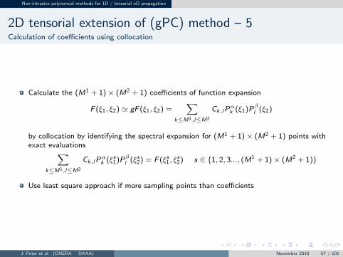
Calculate the (M1 + 1)× (M2 + 1) coefficients of function expansion

F (ξ1, ξ2) ' gF (ξ1, ξ2) =∑

k≤M1,l≤M2


by collocation by identifying the spectral expansion for (M1 + 1)× (M2 + 1) points withexact evaluations∑

k≤M1,l≤M2

Ck,lPαk (ξs1)Pβl (ξs2) = F (ξs1, ξ

s2) s ∈ 1, 2, 3..., (M1 + 1)× (M2 + 1)

Use least square approach if more sampling points than coefficients



2D tensorial extension of (gPC) method – 6Stochastic post processing

gPC 2D expansion

gF (ξ1, ξ2) =∑

k≤M1,l≤M2


Calculation of mean

E(gF ) =

∫ ∑k≤M1,l≤M2


dξ1dξ2 = C0,0


V (gF ) = E((gF − C0,0)2)

=

∫ ∑k≤M1,l≤M2

Ck,lPαk (ξ1)Pβl (ξ2)D(ξ1, ξ2)dξ1dξ2 − C0,0

2

D(ξ1)αDβ(ξ2)dξ1dξ2

=

∫ ∑k≤M1,l≤M2 (k,l)6=(0,0)


2

D(ξ1)αD(ξ2)βdξ1dξ2

=∑

k≤M1,l≤M2 (k,l)6=(0,0)

C 2k,l

Calculation of variance



Stochastic collocation method – 1Definition

Another approach for non-intrusive polynomial chaos based on Lagrangian polynomialexpansion. [Tatang 1995] [Xiu et al. 2005], [Loeven et al. 2007] for compressible CFD

Dedicated stochastic polynomial expansion using Lagrangian polynomials

W (i , ξ) ' scW (i , ξ) =l=M+1∑l=1

Wl (i)Hl (ξ) Hl (ξ) =m=M+1∏

m=1,m<>l

(ξ − ξm)

(ξl − ξm)

(sum of polynomials of degree M)

Note that

scW (i , ξl ) =l=N∑l=1

Wl (i)Hl (ξl ) = Wl (i)

→ no coefficient calculation step. Compute flows (and extract part of state variables fields)W (i , ξl ) corresponding to the ξl / substitute W (i , ξl ) to Wl (i)

scW (i , ξ) =l=M+1∑l=1

W (i , ξl )Hl (ξ)



Stochastic collocation method – 2Suitable set of points

Polynomial expansion using Lagrangian polynomials

W (i , ξ) ' scW (i , ξ) =l=M+1∑l=1

W (i , ξl )Hl (ξ)

Definition of (ξ1, ξ2, ..., ξM+1) ?

1 M + 1 points of the (M + 1)-point Gaussian quadrature associated to D(ξ) (most often,not absolutely necessary)

2 Any set of (M + 1) distinct points

Calculate mean and variance using the (M + 1)-point Gaussian quadratureassociated to D(ξ). Exact mean and variance. Not so simple formulasCalculate mean and variance using interpolatory quadrature associated to thenodes. Inexact mean and variance.



Stochastic collocation method – 3Mean and variance evaluation 1/3

Stochastic post-processing (mean and variance) done for the expansion scW instead of W – In case the(ξ1, ξ2, ..., ξM+1) are the M + 1 points of the (M + 1)-point Gaussian quadrature associated to D(ξ),the weights being (ω1, ω2, ..., ωM+1)

straightforward evaluation of mean value (degree M polynomial)

E(scW (i, ξ)) =

∫scW (i, ξ)D(ξ)dξ =

m=M+1∑m=1

ωmscW (i, ξm) =m=M+1∑m=1

ωmW (i, ξm)

straightforward evaluation of variance (degree 2M polynomial)

E((scW (i, ξ)− E(scW (i)))2) = E(scW (i, ξ)2)− E(scW (i))2

=

∫scW (i, ξ)2D(ξ)dξ − E(scW (i))2

=m=M+1∑m=1

ωmscW (i, ξm)2 − E(scW (i))2

=m=M+1∑m=1

ωmW (i, ξm)2 −(

m=M+1∑m=1

ωmW (i, ξm)

)2

Both exact from quadrature polynomial exactness.



Stochastic collocation method – 4Mean and variance evaluation 2/3

Stochastic post-processing (mean and variance) done for the expansion scW instead of W – In case the(ξ1, ξ2, ..., ξM+1) are not the M + 1 points of the (M + 1)-point quadrature associated to D(ξ). Notethese Gauss quadrature points (ν1, ν2, ..., νM+1) and the weights (ω1, ω2, ..., ωM+1) (no flow have beencalculated for the νm)

This quadrature is used for evaluations of mean and variance

Evaluation of mean value (degree M polynomial)

E(scW (i, ξ)) =

∫scW (i, ξ)D(ξ)dξ =

M+1∑m=1

ωm scW (i, νm)

Evaluation of variance (degree 2M polynomial)


=


=m=M+1∑m=1

ωm scW (i, νm)2 −(

m=M+1∑m=1

ωmscW (i, νm)

)2

Both exact from quadrature polynomial exactness. No simple expression for scW (i, νm)



Stochastic collocation method – 5Mean and variance evaluation 3/3 (skpd)

Stochastic post-processing (mean and variance) done for the expansion scW instead of W – In case the(ξ1, ξ2, ..., ξM+1) are not the M + 1 points of the (M + 1)-point Gaussian quadrature associated toD(ξ)

Interpolatory quadrature associated to the set is used (it is NOT associated to distribution D and Dterms will remain). Weights are denoted (γ1, γ2, ..., γM+1)

In general, inexact evaluation of mean value (due to D factor)

E(scW (i, ξ)) =

∫scW (i, ξ)D(ξ)ξ '

M+1∑m=1

γl scW (i, ξl )D(ξl ) =M+1∑m=1

γl W (i, ξl )D(ξl )

In general, inexact evaluation of variance (due to D factor and polynomial degree)


=


'm=M+1∑m=1

γl scW (i, ξl )2D(ξl )−

(M+1∑m=1

γl W (i, ξl )D(ξl )

)2



2D tensorial extension of (SC) method – 1Definition (1/2)


D(ξ1, ξ2) = Dα(ξ1)Dβ(ξ2)

For the sake of simplicity presented for a scalar output

For the sake of simplicity, tensorial grid of (M1 + 1) and (M2 + 1) Gauss-points associatedto Dα and Dβ .

(ξα1 , ξα2 , ..., ξ

αM1+1

)× (ξβ1 , ξβ2 , ..., ξ

β

M2+1)

the weights being

(ωα1 , ωα2 , ..., ω

αM1+1

) (ωβ1 , ωβ2 , ..., ω

β

M2+1)

Lagrange polynomials associated to the two sets

Hαk (ξ1) =m=M1+1∏

m=1,m<>k

(ξ1 − ξαm)

(ξαk − ξαm)Hβl (ξ2) =

m=M2+1∏m=1,m<>l

(ξ2 − ξβm)

(ξβl − ξβm)



2D tensorial extension of (SC) method – 2Definition (2/2)


D(ξ1, ξ2) = Dα(ξ1)Dβ(ξ2)

Hαk (ξ1) Hβl (ξ2) Lagrange polynomials associated to the two sets of (M1 + 1) (resp.

(M2 + 1)) Gauss quadrature points associated to Dα (resp. Dβ)

Stochastic collocation 2D expansion

scF (ξ1, ξ2) =∑

k≤M1;l≤M2

dk,lHαk (ξ1)Hαl (ξ2) scF (ξ1, ξ2) ' F (ξ1, ξ2)

Identification of the coefficients dk,l = F (ξαk , ξβl )

scF (ξ1, ξ2) =∑

k≤M1;l≤M2

F (ξαk , ξβl )Hαk (ξ1)Hβl (ξ2)



2D tensorial extension of (SC) method – 3

The tensor product of the two Gaussian rules is∫F (ξ1, ξ2)Dα(ξ1)Dβ(ξ2)dξ1dξ2 =

∑k≤M1+1;l≤M2+1


βl )

It exactly integrates all monomials ξp1 ξq2 such that p ≤ 2M1 + 1 q ≤ 2M2 + 1

Calculation of the mean of scF∫scF (ξ1, ξ2)Dα(ξ1)Dβ(ξ2)dξ1dξ2 =

∑k≤M1+1;l≤M2+1

ωαk ωβl scF (ξαk , ξ

βl )

but simply scF (ξαk , ξβl ) = F (ξαk , ξ

βl ) and

E(scF ) =

∫scF (ξ1, ξ2)Dα(ξ1)Dβ(ξ2)dξ1dξ2 =

∑k≤M1+1;l≤M2+1


βl )



2D tensorial extension of (SC) method – 4

The tensor product of the two Gaussian quadratures∫F (ξ1, ξ2)Dα(ξ1)Dβ(ξ2)dξ1dξ2 =

∑k≤M1+1;l≤M2+1


βl )

Calculation of the mean of scF (exact due to polynomial degree)

E(scF ) =

∫scF (ξ1, ξ2)Dα(ξ1)Dβ(ξ2)dξ1dξ2 =

∑k≤M1+1;l≤M2+1


βl )

Calculation of the variance scF (exact due to polynomial degree)

V (scF ) = E((scF − E(scF ))2) = E(scF 2)− E(scF )2

=

∫scF (ξ1, ξ2)2Dα(ξ1)Dβ(ξ2)dξ1dξ2 − E(scF )2

=∑

k≤M1+1;l≤M2+1


βl )2 −

∑k≤M1+1;l≤M2+1


βl )

2



d-D tensorial generalized polynomial choas (gPC) andstochstic collocation (SC) method

Assume same number of collocation or (Gaussian) quadrature points in all directions M

Calculation of polynomial expansion in dimension d requires Md CFD calculations

Not sustainable if d is high. Example with 9 points per direction. Required number ofsimulations

92 = 81 94 = 6561 95 = 59049 96 = 531441 98 = 43.046721 910 = 3.486.784401

feasible up to d = 4 or 5

Introdution of polynomial limited by total degree, t (straightforward)

Bound the total degree t of the polynomial instead of limiting the individual degree in eachvariable. Number of terms of the basis

Z =

(d + tt

)

Introdution of Smolyak sparse quadratures often called sparse grids (not so simple)


Introduction to Smolyak’s sparse quadratures

Outline






6 Conclusions



Smolyak sparse grids – 1Tensorial product of two quadrature rules (Reminder)

2D case

A[f ] =m∑i=1

ai f (xi ) B[f ] =n∑

i=1

bi f (yi ),

A⊗ B[g ] =m∑i=1

n∑j=1

aibj g(xi , yj ),

Straighforward extension to nD

A1 ⊗ A2 ⊗ ...⊗ Ad [f ] =

n1∑i1=1

...

nd∑id=1

w1i1 ...wdid f (x1i1 , ..., xdid )



Smolyak sparse grids – 2Hierarchy of 1D qudratures. Difference of 1D quadratures

1D hierachy of quadratures denotes Ql with increasing number of points. Assumed to beused in all directions

Nested (= quadrature points of points Ql include the quadrature points of Ql−1) or notnested

Difference in successive quadratures

∆k [f ] := Qk [f ]− Qk−1[f ]

Q0[f ] := 0.

Rewriting of a tensor quadrature

Ql1 ⊗ ...⊗ Qld [f ] =∑

k/ 1≤kj≤lj

(∆k1⊗ ...⊗∆kd )

2D illustration

Q3 ⊗ Q2[f ] = (Q3 − Q2)⊗ (Q2 − Q1)[f ] + (Q3 − Q2)⊗ (Q1 − Q0)[f ] +

(Q2 − Q1)⊗ (Q2 − Q1)[f ] + (Q2 − Q1)⊗ (Q1 − Q0)[f ] +

(Q1 − Q0)⊗ (Q2 − Q1)[f ] + (Q1 − Q0)⊗ (Q1 − Q0)[f ]



Smolyak sparse grids – 3Smolyak sparse quadratures (1/2)

Fundamental rewriting of a tensor quadrature

Ql1 ⊗ ...⊗ Qld [f ] =∑

k/ 1≤kj≤lj

(∆k1⊗ ...⊗∆kd )[f ]

Definition of Smolyak sparse quadrature of level l

Qdl [f ] =

∑|k|1≤l+d−1

(∆k1⊗ ...⊗∆kd )[f ]

Very general construction refering to the indices of the 1D quadratures in the hierarchy(not degree, not polynomial exactness...)



Smolyak sparse grids – 4Smolyak sparse quadratures (2/2)

Definition of Smolyak sparse quadrature of level l

Qdl [f ] =

∑|k|1≤l+d−1

(∆k1⊗ ...⊗∆kd )[f ]

Other expressions of Smolayk sparse grids with difference of quadratures

Qdl [f ] =

d+l−1∑j=d

∑k/|k|1=j

(∆k1⊗ ...⊗∆kd )[f ]

Qdl+1[f ] = Qd

l [f ] +∑

k/|k|1=d+l

(∆k1⊗ ...⊗∆kd )[f ]

Direct expressions of Smolayk sparse grids with quadratures

Qdl [f ] =

∑max(l,d)≤|k|1≤l+d−1

(−1)l+d−|k|1−1

(d − 1|k|1 − l

)(Qk1

⊗ ...⊗ Qkd )[f ]



Smolyak sparse grids – 5Polynomial exactness (1/2)

Tensorial product of 1D polynomials

d⊗i=1

P1si

= (x1, ..., xd ) ∈ Rd →d∏

i=1

pi (xi ) ∈ R, pi ∈ P1si

where P1si

is the set of mono-variable polynomials of degree lower or equal to si

The i-th quadrature of the 1D hierarchy Qi is assumed to have polynomial exactness mi

such that mi ≤ mi+1

The Smolyak sparse grid quadrature

Qdl [f ] =

∑|k|1≤l+d−1

(∆k1⊗ ...⊗∆kd )[f ]

is exact for all polynomials of the non classical space

V(Qdl ) = SpanP1

mk1⊗ ...⊗ P1

mkd/ |k|1 = l + d − 1



Smolyak sparse grids – 6Polynomial exactness (2/2)

Example: Series (n/n + 2) nested rules U1, U2, U3, U4 involving n1 = 1, n2 = 3, n3 = 5,n4 = 7 points and having polynomial exactness m1 = 0, m2 = 2, m3 = 4, m4 = 6

Polynomial exactness of Smolyak sparse grid U24

U24 [f ] =

5∑j=2

∑k/|k|1=j

(∆k1⊗∆k2

)[f ]

U24 [f ] = (U4 ⊗ U1 + U3 ⊗ U2 + U2 ⊗ U3 + U1 ⊗ U4 + ...lower .. order...)[f ]

From previous slide, U24 is exact for polynomial vector space V(U2

4 )

V(U24 ) = SpanPm4 ⊗ Pm1 + Pm3 ⊗ Pm2 + Pm2 ⊗ Pm3 + Pm1 ⊗ Pm4,

that isV(U2

4 ) = SpanP6 ⊗ P0 + P4 ⊗ P2 + P2 ⊗ P4 + P0 ⊗ P6.



Smolyak sparse grids – 7Number of evaluations, bounds for weights, error analysis

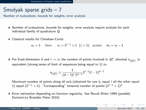
Number of evaluations, bounds for weights, error analysis require analysis for eachindividual family of quadrature Qi

Classical results for Clenshaw-Curtis

n1 = 1 then ni = 2i−1 + 1 (i > 1) points mi = ni − 1

For fixed dimension d and l →∞ the number of points involved in Qdl , denoted n(Qd

l), is

equivalent (strong sense of limit of sequences being equal to 1) to

n(Qdl

) '1

(d − 1)! 2d−12l−1(l − 1)d−1

Maximum number of points along all axis (obtained for one kj equal l all the other equal

1) equal (2l−1 + 1). “Corresponding” tensorial number of points (2l−1 + 1)d

Error estimation depending on function regularity. See Novak Ritter 1999 (possiblyDumont-Le Brazidec Peter 2018)


Examples of application

Outline






6 Conclusions



FG5 generic missile – 3 uncertain parametersNominal mesh at the wall

Generic missile FG5.ONERA experiments. RANS CFD3 uncertain parameters exercise. Angle of attack α, upper fin angle, upper finpositionThree outputs of interest. Side force (CYA), rolling moment (CLA), yawingmoment (CNA)Joint ONERA, DLR, USAF exercise. AIAA paper 2017-1197



FG5 generic missile – 3 uncertain parametersFlow conditions. Uncertain parameters

Nominal flow conditions M = 0.8 α = 12o ReD = 0.6 106

Output of interest : rolling moment, yawing moment, side forceUncertain parameters

Angle of attack in [10o , 14o ]

dα′ = (α− 12)/2 Ds2(dα′) =15

16(1− dα′2)2

Change in upper fin azimutal position in [−1o , 1o ]

dφ = φ− 22.5 Ds3(dφ) =35

32(1− dφ2)3

Upper fin angle in [−1o , 1o ]

Ds3(ξ) =35

32(1− ξ2)3

Joint probability of the three uncertain parameters

D(dα′, dφ, ξ) = Ds2(dα′)Ds3(dφ)Ds3(ξ) =15

16

352

322(1−dα′2)2(1−dφ2)3(1−ξ2)3



FG5 generic missile – 3 uncertain parametersOutputs of interest as function AoA



FG5 generic missile – 3 uncertain parametersNominal flow (1/2)



FG5 generic missile – 3 uncertain parametersNominal flow (2/2)



FG5 generic missile – 3 uncertain parameters

Comparison of nominal flows

DLR Calculations with TAU, USAF caclulations with AVUS, ONERAcalculations with elsAComparison of Kp on the fins and rear part of the missile, comparison ofstagnation pressure in vertical planesThe three flow solutions match well. Good starting point for (UQ) study

Individual variation of outputs w.r.t. parameters

CYA, CLA, CNA non linear as function of α as in the experimentCYA, CLA, CNA linear as function of fin angleCYA, CLA, CNA linear as function of fin position



FG5 generic missile – 3 uncertain parametersFin deformation

(the two mesh deformations can be combined)



FG5 generic missile – 3 uncertain parametersStrategies for UQ

ONERA

3D quadrature = 31-point Smolyak sparse grid based on (1D) Fejer secondrule.31 flow calculations. Classical checks

Quadrature exactly integrates degree 3 polynomials in dimension 3... butD(dα′, dφ, ξ) is a degree 16 polynomialConsidered quadrature fails to correctely integrate D(dα′, dφ, ξ)

Kriging fitted to the 31 evaluations of CLA. Corresponding surrogates forCYA, CNACalculation of mean value and variance based on Riemann sums for (surrogate× D(dα′, dφ, ξ))




DLR

76 TAU simulations budget (actually 8, 16, 32,88, 64 then 76 performingintermediate statistics)Three Kriging surrogates fitted to the 8 then 16... then 76 CLA, CYA, CNAvaluesOne million Monte-Carlo sample built from the cumulative density functions ofDs2(dα′), Ds3(dφ) and Ds3(ξ)Monte-Carlo mean and variance for the Kriging surrogates based on theD(dα′, dφ, ξ)-consistent sampling(Visual) pdf of outputs

ONERA - DLR

Checking individual variations of CLA, CYA, CNA w.r.t. ONERA calculationsshowed differences in slopes → differences in variance expected.




USAF

10 simulations budgetDoE = corners of the parameters domain plus two face centersQuadratic surrogateAnalysis of variance based on the quadratic surrogate



FG5 generic missile – 3 uncertain parameters

More difference in standard deviation than in mean (than visually looking at Kp)



RAE2822 – 3 uncertain parametersNominal mesh at the wall

RAE2822.

RAE experiments.

Case 6. Flow conditions M∞ = 0.725, α = 2.92o, Re = 6.50 · 106

RANS calculations. Outputs of interest CD , CL, CM

Uncertainties on free-stream Mach number M∞, angle of attack α, thickness to chordratio r = h/c

AIAA Paper 2016-433 E. Savin et al.

a = b Xm XM

ξ1 4 0.97× r 1.03× rξ2 4 0.95×M∞ 1.05×M∞ξ3 4 0.98× α 1.02× α

βI(x ; a, b) = 1[Xm,XM ](x)Γ(a + b)

Γ(a)Γ(b)

(x − Xm)a−1(XM − x)b−1

(XM − Xm)a+b−1



RAE2822 – 3 uncertain parametersMesh



RAE2822 – 3 uncertain parametersMesh

0 0.1 0.2 0.3 0.4 0.5 0.6 0.7 0.8 0.9 1−1.5

−1

−0.5

0

0.5

1

1.5

x

Cp

Experimental

Numerical



RAE2822 – 3 uncertain parametersgPC expansion of outputs of interest

gPC expansion. Normalized 1D Jacobi-polynomials ψ orthornormal for

< ψj , ψk >=

∫ +1

−1ψj (ξ)ψk (ξ)

35

32(1− ξ2)3dξ = δjk

Multivariate polynomials involved in the R3 → R1 expansions of CD , CL, CM

ψj(ξ) =3∏

d=1

ψjd (ξd ) |j|1 = j1 + j2 + j3 ≤ t

Total degree t is 8. Dimension is d=3. Number of term in the polynomial expansion is

Z =

(t + dd

)=

(8 + 3

3

)=

(113

)= 165

CD gPC expansion

gCD(ξ1, ξ2, ξ3) =∑

|j|1=j1+j2+j3≤8

cj ψj1 (ξ1) ψj2 (ξ2) ψj3 (ξ3)




1D base-quadrature = p-point Gauss-Jacobi-Lobatto quadrature. Polynomialexactness degree (2p-3)

3D quadratures

Tensorial = Tensorial product of the 10-point Gauss-Jacobi-Lobattoquadrature.Polynomial exactness up to degree 17 for each variable ξj . Exact integration ofproducts of degree 8 polynomials. Exact variance of gPC expansions.Number of points 1000 (103)

Smolyak sparse quadrature = 7-th level Smolyak sparse grid based on thefamily of Gauss-Jacobi-Lobatto quadraturesNumber of points 201



RAE2822 – 3 uncertain parametersVisualization of quadrature points

Figure: Visualization of 6-point tensorial Gauss-Jacobi-Lobatto quadrature and 7th levelSmolyak quadrature based on Gauss-Jacobi-Lobatto quadratures – gPC coefficients arecalculated with 10-point tensorial GJL and 7th level Smolyak quadrature based on GJL




Calculation of the GPC coefficients as (for cD )

cj =

∫ψj(ξ)CD (ξ)D(ξ)dξ

=

∫ψj1

(ξ1) ψj2(ξ2) ψj3

(ξ3)CD (ξ1, ξ2, ξ3)353

323(1− ξ2

1)3(1− ξ22)3(1− ξ2

3)3dξ1dξ2dξ3

First two moments of the aerodynamic coefficients computed by the 10–th level product rule (1000points)

µ σ

CD 133.37e-04 34.128e-04CL 72.274e-02 1.6695e-02CM -453.99e-04 32.239e-04

First two moments of the aerodynamic coefficients computed by the 7–th level sparse rule (201 points)

µ σ

CD 133.38e-04 34.097e-04CL 72.269e-02 1.6729e-02CM -453.96e-04 32.175e-04



RAE2822 – 3 uncertain parametersgPC compressed sensing (1/4)

Reminder: calculation of gPC coefficients by collocation.

Presentation in case of a multi-variate polynomial of fixed total order

Identify F (ξ) and gF (ξ) for Q values of ξ.∑|j|1≤t

CjPj(ξk ) = F (ξk ) ∀ k ∈ 1...q

Matrix notation F column vector of F values, C column vector of unknown polynomialcoefficients K matrix Ki ind(j) = Pj(ξi )

KC = F

Square linear system if number of evaluations = dimension polynomial basis

Least square system if number of evaluations > dimension polynomial basis

Possible use of compressed sensing if number of evaluations < dimension polynomialbasis




Collocation linear system. Identify F (ξ) and gF (ξ) for q values of ξ.

F (ξk ) =∑|j|1≤t

CjPj(ξk ) ∀ k ∈ 1...q

or in matrix notationKC = F

K has q lines (number of evaluations) and Z columns (number of polynomials in the basis)

May be solved with less information (evaluations) than unkowns (gPC coefficients) by

compressed sensing provided

The actual gPC expansion that is looked for is sparse = has many coefficientsvery close to 0. This is often the case. This is called “sparsity of effects”This is verfied for the searched expansionRequires a (random) sampling incoherent with basis of polynomial that ismeasured by the “mutual coherence”

max1 ≤ j, l ≤ Z

j 6= l

|KTj Kl |

‖Kj‖2‖Kl‖2

that should have the lowest possible value




Collocation linear system. Identify F (ξ) and gF (ξ) for q values of ξ.

F (ξk ) =∑|j|1≤t

CjPj(ξk ) ∀ k ∈ 1...q

In matrix notationKC = F

The underdetermined problem is then solved by L1 minimization

C∗ = arg minh∈RZ

‖h‖1; ‖ Kh− F‖2 ≤ ε




165 polynomals in the basis

80 random sampling points

Mutual coherence equal 0.93

Good recovery of mean and variance with compressed sensing gPC :

µ σ

CD 133.33e-04 34.052e-04CL 72.271e-02 1.6703e-02CM -453.95e-04 32.180e-04


Conclusions

Outline






6 Conclusions


Conclusions

Way forward...

Uncertainty quantification

needed for robust analysis, robust design, validationmore and more interest and projects (EU, RTO...)

Way to proceed

Get precise definition of industry relevant problemsUse both mechanical and mathematical test cases

ChallengesDeal with large numbers of uncertain parameters

Use sensitivity analysis (Sobol indices...)Use sparsity of effects

Deal with geometrical uncertainties


Generalized polynomial chaos and stochastic collocation … · 2019-01-14 · Generalized...

Documents

Transcript of Generalized polynomial chaos and stochastic collocation … · 2019-01-14 · Generalized...