UNBONDED MONOSTRANDS FOR CAMBER … · 2.5.3.1 NCHRP 496 Shrinkage Model..... 23 2.5.4 Prestressing...

UNBONDED MONOSTRANDS FOR CAMBER ADJUSTMENT

by

Vivek Sethi

Thesis presented to the faculty of the

Virginia Polytechnic Institute and State University

In partial fulfillment of the requirements for the degree of

Master of Science

in

Civil Engineering

Committee:

Carin L. Roberts-Wollmann, Co-Chair

Kamal B. Rojiani, Co-Chair

Richard E. Weyers

Feb 13, 2006

Blacksburg, VA

Keywords: Camber, Creep, Shrinkage, High strength concrete, Monte Carlo Simulation,

Prediction models, Probability distribution, Unbonded monostrands

Copyright 2006 Vivek Sethi

iii

UNBONDED MONOSTRANDS FOR CAMBER ADJUSTMENT

Vivek Sethi

Abstract

Prestressed concrete structural members camber upwards or downwards depending upon

the location of application of prestress force. Identical members do not camber equally

due to variability of the factors influencing it. Differential camber in the beams, if

significant, results in excessively tall haunches or girder top flange extending into the

bottom of the slab. For adjacent members like deck bulb-tees and box girders that are to

be transversely post-tensioned the differential camber causes problems during the fit up

process. This variation is undesirable and hinders the smooth progress of construction

work if not properly accounted for at the design stage.

Various factors influence camber and camber growth in prestressed members. Some of

the factors are concrete strength and modulus, concrete creep and shrinkage properties,

curing conditions, maturity of concrete at release of prestress force, initial strand stress,

climatic conditions in storage and length of time in storage. Combinations of these

variables result in variation of camber of otherwise similar beams at the time they are

erected.

One way to increase the precision of camber estimation is to use Monte Carlo simulation

based upon the randomized parameters affecting the camber and camber growth. In this

method, the parameters, in the form of a probability distribution function, are combined

and passed through a deterministic model resulting in camber and camber growth

prediction with narrowed probability bounds as compared to single definite value given

by most contemporary methods. This outcome gives the expected range of cambers for a

given girder design. After determining the expected range of camber, the ultimate goal is

to provide guidelines for using unbonded monostrands for camber adjustment.

iv

ACKNOWLEDGEMENT

Saying a thank you would not fully express my gratitude toward my professors who have

been my mentors and guides for the last one and a half years. I would like to thank

especially my committee chair and advisor Dr. Carin L. Roberts-Wollmann who showed

faith in my capabilities and gave me an opportunity to work on this project. She was a

constant source of inspiration and guidance and was always there to answer my every

question. I would also like to thank my committee co-chair Dr. Kamal B Rojiani, without

whose expertise and guidance in Statistical methods, this work would not have been a

reality. I would also like to thank Dr. Richard E. Weyers for serving as a member of my

committee and for his guidance on concrete materials.

I would like to express my gratitude toward my mother Sumitra Sethi, father VK Sethi,

sister Swati and brother-in-law Harsh, without whose financial and emotional support, I

could never be the person I am now.

I would like to say a special thanks to my roommate Surya, whose constant motivation

and good food kept me working for long hours. I would like to thank my friends Manoj,

Hasan, Ravi, Sumit, Vyas, for their encouragement and support.

Last but not least, I would like to thank God for giving me patience and perseverance to

fulfill my dreams.

iii

Table of Contents

List of tables......................................................................................................................vii

List of figures…………………………………………………………………………….ix

Chapter 1............................................................................................................................. 1 Introduction......................................................................................................................... 1

1.1 Introduction............................................................................................................... 1 1.2 Implementing a Probabilistic Analysis ..................................................................... 2

1.2.1 Transformed Section Analysis........................................................................... 2 1.2.2 Monte Carlo Applications.................................................................................. 3

1.3 Objective and Scope ................................................................................................. 3 1.4 Organization.............................................................................................................. 4

Chapter 2............................................................................................................................. 5 Literature review................................................................................................................. 5

2.1 Introduction............................................................................................................... 5 2.2 Problems with Prestressed Concrete......................................................................... 6 2.3 Prestress Losses ........................................................................................................ 6 2.4 Camber...................................................................................................................... 9 2.5 Parameters Affecting Camber................................................................................. 12

2.5.1 Modulus of Elasticity....................................................................................... 12 2.5.1.1 AASHTO LRFD Specification ..................................................................... 13 2.5.1.2 ACI 363......................................................................................................... 14 2.5.1.3 ACI 318......................................................................................................... 14 2.5.1.4 NCHRP 496 .................................................................................................. 14

2.5.2 Creep .................................................................................................................... 15 2.5.2.1 Mathematical Model of Creep of Concrete .................................................. 17 2.5.2.2 NCHRP 496 Creep Model ............................................................................ 19

2.5.3 Shrinkage ............................................................................................................. 21 2.5.3.1 NCHRP 496 Shrinkage Model...................................................................... 23

2.5.4 Prestressing Steel Relaxation............................................................................... 24 2.5.5 Age at Release...................................................................................................... 26 2.5.6 Thermal Effects.................................................................................................... 26 2.6 Monte Carlo Method............................................................................................... 27

2.6.1 Theory of Monte Carlo Method....................................................................... 27 2.6.2 Monte Carlo Approximation of Exact Integrals .............................................. 29

2.7 Conclusions............................................................................................................. 30 Chapter 3........................................................................................................................... 31 Method of Analysis........................................................................................................... 31

3.1 Introduction............................................................................................................. 31 3.2 Description of Model .............................................................................................. 32

3.2.1 Instantaneous Deflections (Phase 1) ................................................................ 33 3.2.2 Time Dependent Camber Changes (Phase II).................................................. 36

3.3 Program Operation.................................................................................................. 38 3.4 Implementing the Monte Carlo Procedure.............................................................. 38

iv

3.5 Member Modeling and Input .................................................................................. 39 Chapter 4........................................................................................................................... 42 Statistical Parameters and Random Number Generation.................................................. 42

4.1 Introduction............................................................................................................. 42 4.2 Statistical Parameters .............................................................................................. 42

4.2.1 Concrete Strength Variability .......................................................................... 42 4.2.2 Variability of Prestressing Steel Parameters.................................................... 43 4.2.2.1 Modulus of Elasticity of Prestressing Steel .................................................. 43 4.2.2.2 Prestressing Steel Area ................................................................................. 43 4.2.2.3 Depth of Prestressing Strands ....................................................................... 44 4.2.2.4 Ultimate Tensile Strength of Prestressing Steel............................................ 44 4.2.2.5 Jacking Stress in Prestressing Strands .......................................................... 45

4.2.3 Ultimate Shrinkage Coefficient ........................................................................... 45 4.2.4 Ultimate Creep Coefficient .................................................................................. 46 4.2.5 Curing Time and Loading Age ............................................................................ 46 4.2.6 Humidity .............................................................................................................. 46 4.2.7 Cross Sectional Area............................................................................................ 47 4.2.8 Perimeter .............................................................................................................. 47 4.2.9 Moment of Inertia ................................................................................................ 47 4.2.10 Ratio of Volume to Surface Area....................................................................... 47 4.2.11 Unit Weight of Concrete.................................................................................... 48 4.3 Practical Application of Theory of Monte Carlo .................................................... 48

4.3.1 Variance Reduction Techniques ...................................................................... 48 4.3.2 Transformation of Variables ............................................................................ 50 4.3.3 Random Number Generator............................................................................. 50 4.3.4 Rejection Techniques....................................................................................... 51

Chapter 5........................................................................................................................... 54 Evaluation of Variability of Camber in Prestressed Concrete Bridge Girders ................. 54

5.1 Introduction............................................................................................................. 54 5.2 Parametric Study..................................................................................................... 54 5.3 Comparison of Field Data....................................................................................... 61 5.4 Sensitivity Analysis ................................................................................................ 68 5.5 Feasibility Study for Using Unbonded Monostrands.............................................. 72

Chapter 6........................................................................................................................... 81 Findings and Recommendations ....................................................................................... 81

6.1 Findings................................................................................................................... 81 6.2 Recommendations for Future Research .................................................................. 83

References......................................................................................................................... 85 APPENDIX A................................................................................................................... 90 APPENDIX B ................................................................................................................. 114 APPENDIX C ................................................................................................................. 117

C.1.1 Assumptions ...................................................................................................... 118 C.1.2 Feasibility Check for Anchorage Arrangement in the PCBT Girder with No Draped Strands............................................................................................................ 118

C.1.2.1 Vertical Bearing Plates............................................................................... 118 C.1.2.2 Bearing Stresses Behind Vertical Anchorages........................................... 119

v

C.1.2.3 Horizontal Bearing Plates........................................................................... 121 C.1.2.4 Bursting Reinforcement ............................................................................. 121 C.1.2.5 Bearing Stress Behind Horizontal Anchorage ........................................... 122 C.1.2.6 Compressive Stress at the End of Local Zone............................................ 122

C.1.3 Feasibility Check for Anchorage Arrangement in PCBT Girder with Draped Strands......................................................................................................................... 123

C.1.3.1 Bearing Stress Behind Horizontal Anchorage ........................................... 123 C.1.3.2 Compressive Stress at the End of Local Zone............................................ 124

C1.4 Camber Control Using Unbonded Monostrands................................................ 124 VITA............................................................................................................................... 128

vi

List of Tables

Table 4.1-Camber parameters and their statistical distributions…………………………53

Table 5.1-Comparison between Deterministic and Probabilistic solution of camber at

release for PCBT 29 girder………………………………………………………………56

















Table 5.10-Field data provided by Bayshore Concrete for a PCBT 45 girder………......62

Table 5.11-Comparison of predicted range of camber at release values to experimentally

measured camber at release……………………………………………………………...63

Table 5.12-Comparison between the MCS predicted values and experimentally measured

values of camber at release and camber growth for Cooper River bridge girders………68

Table 5.13-Results of Sensitivity Study…………………………………………………70

Table 5.14-Comparison between expected variation and correction achieved due to

unbonded monostrands for PCBT 29 girder…………………………………………….76


unbonded monostrands for PCBT 37 girder……………………………………………..76

vii















Table A.1-Details for number of strands used in PCBT sections………………………113

Table B1-Data of beams in Sample 1……………………………….…..……………...115

Table B2-Data of beams in Sample 2…………………………………...……………...116

viii

List of figures

Figure 2.1-Stress versus time in the strands in a pretensioned concrete girder……….......8

Figure 2.2-Elastic components of beam camber and deflection immediately after

release……………………………………………………………………………………10

Figure 2.3-Components of time dependent camber and deflection……………………...11

Figure 5.1-Graph showing the probability density function of camber at release for beam

number 1…………………………………………………………………………………61

Figure 5.2-Dimensions of the 79 in. modified bulb tee used in the Cooper River Bridge,

Charleston………………………………………………………………………………..64


sample 1………………………………………………………………………………….65

Figure 5.4-Graph showing the probability density function of camber growth at 60 days

for beam sample 1………………………………………………………………………..65


sample 2………………………………………………………………………………….66

Figure 5.6-Graph showing the probability density function of camber growth at 60 days

for beam sample 2………………………………………………………………………..66

Figure 5.7-Graph showing the probability density function of final camber at 60 days for

beam sample 1……………………………………………………………………………67

Figure 5.8-Graph showing the probability density function of final camber at 60 days for

beam sample 2……………………………………………………………………………67

Figure 5.9-Sketch showing the arrangement of Type S6 monostrand anchorages in a

PCBT girder having no draped strands…………………………………………………..73

Figure 5.10-Sketch showing the arrangement of Type S6 monostrand anchorages in a

PCBT girder having draped strands……………………………………………………...73

Figure A.1-Graph showing the probability density function of camber at release for beam

number 1…………………………………………………………………………………91

Figure A.2-Graph showing the probability density function of camber growth at 90 days

for beam number 1……………………………………………………………………….91

ix


number 2…………………………………………………………………………………92


for beam number 2……………………………………………………………………….92


number 3…………………………………………………………………………………93


for beam number 3……………………………………………………………………….93


number 4…………………………………………………………………………………94


for beam number 4……………………………………………………………………….94


number 5…………………………………………………………………………………95


for beam number 5……………………………………………………………………….95

Figure A.11-Graph showing the probability density function of camber at release for

beam number 6…………………………………………………………………………...96


for beam number 6……………………………………………………………………….96


beam number 7…………………………………………………………………………...97


for beam number 7……………………………………………………………………….97


beam number 8…………………………………………………………………………...98


for beam number 8…………………………………………………………………….....98


beam number 9...…………………………………………………………………………99

x


for beam number 9……………………………………………………………………....99


beam number 10..……………………………………………………………………….100


for beam number 10..…………………………………………………………………...100


beam number 11………….……………………………………………………………..101


for beam number 11…..………………………………………………………………...101


beam number 12………….……………………………………………………………..102


for beam number 12…..………………………………………………………………...102


beam number 13………….……………………………………………………………..103


for beam number 13…..………………………………………………………………...103


beam number 14………….……………………………………………………………..104


for beam number 14…..………………………………………………………………...104


beam number 15………….……………………………………………………………..105


for beam number 15…..………………………………………………………………...105


beam number 16………….……………………………………………………………..106


for beam number 16…..………………………………………………………………...106

xi


beam number 17………….……………………………………………………………..107


for beam number 17…..………………………………………………………………...107


beam number 18………….……………………………………………………………..108


for beam number 18…..………………………………………………………………...108


beam number 19………….……………………………………………………………..109


for beam number 19…..………………………………………………………………...109


beam number 20………….……………………………………………………………..110


for beam number 20…..………………………………………………………………...110


beam number 21………….……………………………………………………………..111


for beam number 21…..………………………………………………………………...111

Figure A.43 Dimension details of a PCBT sections used by VDOT…………………...112

Figure B1 Strand Pattern of Sample 1………………………………………………….115

Figure B1 Strand Pattern of Sample 2………………………………………………….116

Figure C.1 Data sheet showing the dimension details of type S6 anchorage used……..127

xii

Chapter 1

Introduction

1.1 Introduction

Camber and camber growth are characteristic of all prestress members. Beams are

observed to camber differently even though they have similar dimensions and concrete

properties. This difference in camber of otherwise identical beams poses many problems

during construction like increased haunch depths, jutting of beams into the bottom of the

slab and increase in time for setting up the forms for cast in place deck slabs. Also for

adjacent box girders and deck bulb-tees, the difference in camber causes problems during

the fit up process. This unnecessarily increases the time and cost of construction.

Engineers over the years have improved their understanding of the behavior of concrete,

but have been unable to precisely predict it. Concrete is a very complex material and its

properties depend on materials used and environmental conditions under which it is

produced and stored. These infinite combinations of materials and environmental

conditions render it impossible to model precisely. The camber and camber growth in

prestress members depends on various factors such as concrete strength and modulus,

concrete creep and shrinkage properties, curing conditions, maturity of concrete at release

of prestress force, initial strand stress, climatic conditions in storage and length of time in

storage. Combination of these variable parameters results in variation of camber at the

time of erection.

Lack of proper models to predict the behavior of concrete results in erroneous estimates

of prestress losses and thus the camber in prestressed members. The variability in the

concrete properties calls for the use of probabilistic methods to estimate a range of

camber rather than calculating a discreet value as given by most contemporary methods.

1

The limits of the parameters affecting the camber and camber growth and their statistical

distribution have been determined from experimental tests and published in literature. It

is therefore possible to create a probability distribution function of the camber and

camber growth in structural members based upon the random variation of the parameters

and a model that can combine these parameters to calculate camber. This should give the

range of camber expected for the structural member simulated by the model.

1.2 Implementing a Probabilistic Analysis

The overall analysis in this thesis consists of the application of two methods. The first

being the transformed section analysis of concrete using the age adjusted effective

modulus to plot the moment curvature relationships for calculation of camber and the

second is randomizing the parameters affecting the above analysis using the Monte Carlo

method to generate a probability distribution for the camber and camber growth.

1.2.1 Transformed Section Analysis

The stresses, strains and the prestress losses in the structural members are computed

using either a net concrete section or a transformed section. The advantage of the

transformed section analysis using the age adjusted effective modulus is that prestress

losses are not calculated explicitly but are accounted for intrinsically in the method. The

stresses and strains at various sections in the structural member are calculated using the

transformed section analysis and then the force, moment and curvature in the net concrete

section at various points is calculated. After that, the curvature diagram is plotted and

then using the moment area method the deflection is calculated.

The camber growth is calculated using a change in curvature plot. The change in

curvature is calculated using the age adjusted effective modulus approach by setting the

necessary equilibrium, constitutive and compatibility relationships on the forces in the net

concrete section. The parameters used to calculate the camber and camber growth are

randomized from their probability distribution functions using the Monte Carlo method

2

and the probability distributions of camber and camber growth is generated. This

probability distribution then gives a mean, an upper bound and a lower bound in which

the camber is expected to fall for the member simulated. Thus its helps in establishing a

confidence interval for the camber and camber growth rather than giving a discrete value

as given by contemporary methods.

1.2.2 Monte Carlo Applications

The numerical method known as the Monte Carlo method is a statistical simulation

technique to simulate a random or stochastic process. The Monte Carlo method is often

used in simulations where the number of variables affecting the behavior of a system are

too numerous and not sufficiently well understood for an analytical solution. The only

requirement of the method is that the factors affecting the physical behavior of the system

be described as probability distribution functions. Examples of the implementation of the

Monte Carlo methods in civil engineering include the comparison of prestress loss

methods in prestressed concrete beams (Ahlborn and Glibertson, 2003). Kirkpatrick

(2001) determined the statistics of impact of chloride induced corrosion on service life of

Virginia bridge decks using the Monte Carlo method. MacGregor (1979) used the method

to develop the statistics of shear strength for slender reinforced beams in bending. Monte

Carlo methods are also used in limit state applications where the reliability of high

strength concrete is studied or where the reliability of partially prestressed beams is

studied at those limit states (Naaman et al., 1982). The above examples use the Monte

Carlo method to develop the statistics.

1.3 Objective and Scope

The objectives of this thesis are as follows:

1. To develop a simple probabilistic model for camber and camber growth of

prestressed concrete members based on the transformed section analysis using the

age adjusted effective modulus approach similar to the one used in NCHRP 496().

3

2. To utilize the probabilistic model in Monte Carlo simulation to simulate camber

and camber growth characteristics of commonly used girder types produced by

prestressing plants in Virginia. The probabilistic model should simulate camber

and camber growth characteristics of all possible girder types commonly used in

modern bridges. It is anticipated that the results of the simulation will provide

expected values of camber and camber growth and a range in which they are

expected to fall.

3. To confirm the validity of the model by comparing the results with the actual field

data.

4. To study the feasibility of providing unbonded monostrands at the bottom of the

girder, to adjust the camber upwards, as well as at the top of the girder to adjust

the camber downwards. In addition, the influence of the monostrands tendons on

the girder stresses and ultimate strength will also be studied.

5. To provide recommendations for future work.

1.4 Organization

This thesis is divided into six chapters. The first chapter introduces the problem statement

and briefly describes the approach and the method of analysis used in this thesis. The

second chapter is the theoretical development of the model and briefly reviews the

literature associated with it. The method of analysis is described in the third chapter. The

fourth chapter describes the method of random number generation and the statistics of the

variables describing the model. Results of the simulation are presented in the fifth

chapter. Discussion of these results and recommendations for future work are suggested

in the sixth chapter.

4

Chapter 2

Literature review

2.1 Introduction

Concrete is an excellent compressive material but has poor tensile properties. Its tensile

strength is approximately 10 percent of its compressive strength (Nilson, 1997). The

tensile strength of concrete is unpredictable and is associated with small deformations

prior to failure. These small deformations lead to a brittle failure, which is undesirable in

design from safety and serviceability points of view. Therefore, reinforcing steel bars are

placed in concrete members to improve their tensile performance and make the structure

more ductile. Ordinary reinforcing steel is suitable for short span members. For medium

and long spans, problems like excessive member size, steel quantities beyond those

necessary to ensure ductile failure, and lack of economy are encountered.

The concept of prestressing concrete beams was invented in an effort to reduce excessive

member sizes, span longer distances and improve the serviceability performance of

ordinary reinforced concrete. The most common serviceability problems are crack

widths and deflections. It is observed that crack widths are directly proportional to the

magnitude of stress in reinforcing steel. Thus to limit crack widths, reinforcing steel is

used at a much lower stress than it is capable of withstanding. The problems of large

deflections and crack width are overcome by prestressing the steel at a high stress and

applying most of the steel strain before the member is loaded.

The reasons why prestressed concrete is preferred over reinforced concrete are as

follows:

• Longer spans

• Lighter members

• Efficient use of materials

• Control of cracking

5

• Smaller deflections

• Smaller dead load to live load ratio

• Greater carrying capacity for a given member size.

The development of prestressed concrete is credited to French engineer Eugene

Freyssinet. He noticed the improvement in concrete performance that arises from

prestressing. He was the first person who studied the effects of creep and shrinkage on

prestressed concrete. His studies led him to realize that steel at high initial stress should

be used to ensure that the prestress force lost due to time effects is not greater than the

applied prestress to the steel. Thus, the use of high strength steel in prestressing began.

2.2 Problems with Prestressed Concrete

The use of prestressed concrete is very wide and varied. Its use is becoming more popular

with time and slowly it is becoming a material of choice. In spite of many advances in the

use of prestressed concrete, there have been only small advances in methods of predicting

time dependent losses. There is a need for an all-encompassing model for predicting

creep and shrinkage behavior in concrete, which is simple enough to be used by design

engineers in practical applications. Research is still going on in this area but it is unlikely

that this problem can be solved in near future. The reason that this problem cannot be

solved so easily is the complex nature of concrete. Due to the complexity of predicting

the creep and shrinkage of concrete, various code committees have developed predictive

models which are conservative for design but sacrifice economy and efficiency (Bazant et

al. 1984). It is for this reason that the precast industry and researchers are constantly

endeavoring to develop a better model for the prediction of creep and shrinkage.

2.3 Prestress Losses

Prestress losses are divided into two categories:

• Instantaneous losses

6

• Time dependent losses

Instantaneous losses depend on the method of prestressing used:

In pretensioned concrete, the instantaneous losses are as follows:

• Elastic shortening

In post-tensioned concrete, the instantaneous losses are as follows:

• Frictions losses (curvature and wobble)

• Seating losses

• Elastic shortening (with multiple tendons)

Elastic shortening losses occur because of shortening of concrete in the elastic range due

to applied stress. Friction losses occur only in post tensioning due to the friction between

the tendon and the duct through which it is passed. Seating losses depend on the type of

equipment used by the post-tensioning supplier and most manufacturers of post

tensioning systems specify it as a standard value.

Time dependent losses are independent of the method of prestressing used, and they are

as follows:

• Loss due to creep of concrete

• Loss due to shrinkage of concrete

• Loss due to relaxation of steel strand

• Thermal effects

Thermal effects on long-term prestress losses are neglected in design. They are

significant in the regions where extreme temperature variations occur. Incorporating the

effects of temperature in creep and shrinkage models is very difficult due to the complex

nature of the problem (Bazant, 1985). In normal operating environments, the effect of

temperature is insignificant and therefore it is neglected (Bazant et al. 1983).

For the other time dependent losses, various analytical models are used to predict the

behavior. However, due to the material complexity of concrete, it is very difficult to

develop a comprehensive model for predicting creep and shrinkage effects in concrete

over time. Relaxation of prestressing steel is a type of creep effect and is defined as loss

7

of stress in steel at constant strain. This effect is predicted quite well by its analytical

model because of the homogeneity of material.

Various internationally recognized models are available for predicting creep, shrinkage,

elastic shortening and strand relaxation effects. Each method has its merits and

drawbacks. For this thesis, the model recommended by NCHRP Report 496 (2003) for

predicting creep, shrinkage and elastic shortening are used. The reason for using the

NCHRP Report 496 model is that it is the only model designed specifically for high

strength concrete (HSC) and is already included in the 2005 Interim AASHTO LRFD

specification. The strand relaxation model is the Prestressed Concrete Institute Bridge

Design Manual model (PCI, 1997). The AASHTO LRFD design methods are used in this

thesis for design of girders. Major factors affecting the prestressed concrete and

ultimately the camber are discussed in the following sections. The variation of stress

versus time in a prestressed concrete girder is shown in Fig 2.1

Figure 2.1 Stress versus time in the strands in a pretensioned concrete girder (NCHRP

Report 496, 2003)

8

2.4 Camber

Camber is the upward deflection in flexural members due to an eccentrically applied

prestressing force. Camber is subdivided into two categories i.e., initial camber and long-

term camber. Initial camber is induced at transfer of the prestressing force at the time of

release. It is the net upward deflection calculated by algebraically summing the smaller

downward deflection caused by the beam self weight (∆beam) and the larger upward

deflection (∆ps) caused by the prestressing force applied at an eccentricity ‘e’ below the

center of gravity of the section. The components of camber due to self weight and

prestressing force are given in Eqs. 2.1 and 2.2

45

384s

beamc

wLE I

∆ = (2.1)

2

8s

psc

PeLE I

∆ = (2.2)

for straight tendon profile

The magnitude of initial camber is the difference (∆ps- ∆beam) between the above two

values. Figure 2.2 illustrates the components of initial camber in the beams.

The long-term camber is extremely difficult to predict because of the large variability in

the factors affecting it. Some of the factors affecting the camber growth are concrete

strength and modulus, maturity of concrete at the time of transfer of prestress, creep, and

shrinkage. The time dependent growth of camber is most affected by creep, which is

caused by sustained applied loads such as prestress, and dead weight on the beam as

shown in Figure 2.3.

Various methods are available for predicting initial and long-term camber in girders.

Many studies have been done in the past to verify these methods with experimental

9

a) Loads applied to beam at release

b) Deflections due to beam weight

c) Camber due to prestressing force

Figure 2.2 Elastic components of beam camber and deflection immediately after release

(Byle et al. 1997).

10

Figure 2.3 Components of time dependent camber and deflection (Byle et al. 1997).

11

results. Literature pertaining to these studies has been reviewed and a brief overview of

these studies is given in the following paragraphs.

It has been observed that beams having identical cross sectional dimensions and material

properties have significant variation in their cambers (Stallings et al. 2001). Kelly, Breen

and Bradberry (1987) found that beams made of low strength concrete exhibited the

greatest camber during erection, the greatest time dependent effects, and the least final

camber at the end of their service life whereas beams made of high strength concrete

exhibited opposite trends. Hinkle (2005) measured the camber of beams from the time of

release until an age of 180 days. The experimental results showed the camber to increase

until an age of 40 days, after which it stabilized for the duration of the measurement.

Byle, Burns and Carrasquillo (1997) tracked camber and deflection from the time of

release until the beams were in service. They compared the experimental results with the

PCI method (PCI BDM, 1997) and the time step method (Branson, 1997) and they found

the time step method to be a better predictor of camber when using time dependent

material properties. Stallings and Eskildsen (2001) compared the experimentally

measured values with theoretical values calculated using an incremental time step

method. It was observed that when standard parameters of creep and shrinkage were used

with an incremental time step method, it over predicted the camber by 24 percent. Upon

using the parameters of HSC it under estimated the values by 6 percent on an average

below the measured camber values. The larger error when standard parameters were used

was attributed to over estimation of creep effects.

2.5 Parameters Affecting Camber

2.5.1 Modulus of Elasticity

Researchers over the years have worked to find a simple relationship for the modulus of

elasticity of concrete. Neville (1997) asserted that there could be no simple relationship

between the modulus of elasticity and compressive strength of concrete. The reason for

this is that the modulus of elasticity of concrete is affected not only by the modulus of

12

elasticity of the aggregate but also the volumetric content of the aggregate in the mix.

Current equations of modulus of elasticity given in various codes and specifications do

not account for the bond between the aggregate and cement paste. Upon loading the

concrete, micro cracking occurs at the interface of aggregates and cement paste and it is

observed to affect the structural behavior of concrete. The stress-strain relationship of the

constituent materials is observed to be linear but their combined response in concrete is

nonlinear. The stress strain relationship for concrete is curvilinear and depends on the

relative stiffness of aggregates and cement paste.

Due to the lower water cement ratio (w/c) in HSC mixes, the modulus of elasticity is

found to be similar between the hardened cement paste and aggregate. Thus, concrete

behaves as a more homogeneous material and its stress strain curve approaches linearity.

Baalbaaki, Aitcin and Ballivy (1992) observed that the relationship between the modulus

of elasticity and compressive strength are only valid for normal strength concrete. They

also observed that predicting the modulus of elasticity of concrete based on the modulus

of elasticity of aggregate worked well for granite and limestone aggregates, but not for

quartzite and sandstone aggregates.

Various studies have been done to measure the accuracy of models for prediction of

modulus of elasticity of concrete with the experimental results. The models that have

been studied and a summary of the findings are as follows:

2.5.1.1 AASHTO LRFD Specification

The present AASHTO Equation 5.4.2.4-1 (AASHTO LRFD, 1998) given as Equation

number 2.3 is applicable only for concrete having unit weights of 0.090kcf to 0.155kcf.

1.5 '33000c cE w= cf (kcf and ksi) (2.3)

where Ec is the concrete modulus of elasticity,

fc’ is the concrete compressive strength of 4x8 cylinder at corresponding age, and

wc is the unit weight of concrete.

13

The ACI 363 Committee report (ACI 363, 1992) observed that this equation tends to

significantly over estimate the modulus of elasticity of concretes with compressive

strengths higher than 6 ksi. Huo, Al-Omaishi, and Tadros (2001) observed a similar

trend. NCHRP 496 (2003) also observed a similar trend where the above equation

overestimated the modulus of elasticity for HSC.

2.5.1.2 ACI 363

The ACI 363 (ACI 363, 1992) equation for modulus of elasticity, given as Equation 2.4

below.

( )1.5

'1000 12650.145

cc c

wE f⎛ ⎞= +⎜ ⎟⎝ ⎠

(kcf and ksi) (2.4)

where the Ec, fc’ and wc are same as defined above.

This equation also over predicts the modulus for high strength concrete (Ahlborn et al.

1996). Myers and Carrasquillo (1999) have shown that modulus of elasticity of concrete

appears to be a function of aggregate content and type. The above equation also does not

include factors other than concrete self-weight and strength.

2.5.1.3 ACI 318

ACI 318 (ACI 318, 2002) also uses a similar equation as the AASHTO LRFD Equation

5.4.2.4-1 and similar trends of under prediction of modulus of elasticity have been

reported by various researchers (Kahn et al. 1997).

2.5.1.4 NCHRP 496

This is the most recent equation given for predicting the modulus of elasticity of high

strength concrete. It includes the effect of aggregate type, the equation is given as: 1.5'

'1 233000 0.140

1000c

cf

cE K K f⎛ ⎞

= +⎜ ⎟⎝ ⎠

(ksi) (2.5)

14

where Ec, fc’ have the same meaning as above and

wc= 1.5'

0.1401000

cf⎛ ⎞+⎜ ⎟

⎝ ⎠

K1 = represents the difference between the national average and local average if

test results are available

K2 = represents whether an upper bound or lower bound is required. Note that fc’

is in ksi.

Tadros and Al-Omaishi (2003) have observed that this equation predicts the upper and

lower bounds for the modulus of elasticity of the high strength concrete made in four

states of Nebraska, New Hampshire, Texas and Washington very well. They have also

given values of K1 and K2 depending on the types of aggregates available in these states.

They have suggested that where the values of K1 and K2 are not available they should be

taken as one.

Waldron (2004) measured the prestress losses for nine HSC girders in Virginia and

compared the losses predicted by various methods. He found that the NCHRP 496 (2003)

method to be one of the best predictors. The difference between measured and predicted

losses was less than 5 ksi. This method has been incorporated in the 2005 Interim

AASHTO LRFD Specifications. Thus, in this thesis this model is used for predicting the

modulus of elasticity, creep and shrinkage of concrete.

2.5.2 Creep

Concrete creep is the most significant time and stress dependent effect in concrete.

Considerable research has been done in the field of creep study. Despite this, there is no

all-encompassing model which can predict creep and shrinkage accurately. This is due to

material complexity of concrete, which renders the task of predicting accurately creep

effects in concrete very difficult. Concrete after its formation is not in a state of

equilibrium and undergoes change due to ongoing hydration reaction and moisture

15

diffusion through the member. Therefore, creep is separated in two components, basic

creep and drying creep. Basic creep is the continued deformation under an applied stress

occurring in a sealed specimen in a hydro-equilibrium environment. Drying creep occurs

when a specimen is free to exchange moisture with the environment, inducing a drying

stress in the specimen. In a prestressed girder, creep results in camber growth. The

prolonged shortening of the bottom flange of the girder due to eccentrically applied

prestress force causes the growth of camber in girders. The rate and extent of creep in

prestressed girders depends on factors like time, maturity of the concrete at the time the

time load is first applied, magnitude of applied stress, curing conditions, ambient relative

humidity, mixture proportions, aggregate properties and w/c ratio.

Creep characteristics of concrete depend on the maturity of the concrete at the time it is

first loaded. A more mature concrete specimen has better capacity to resist creep on

application of load. HSC is found to be more sensitive to early age loading than normal

strength concrete (Kahn et al 1997).

The magnitude of applied stress also influences creep characteristics of concrete. ACI

209 (ACI, 1992) suggests that the amount of creep is proportional up to an applied stress

level of 40 percent of concrete strength. Shams and Kahn (2000) have suggested that, for

HSC the amount of creep is proportional up to 60 percent of concrete compressive

strength. According to AASHTO LRFD specifications (AASHTO, 1998) also, concrete

strains are proportional to applied stress equal to 60 percent of concrete compressive

strength.

ACI 209 (ACI, 1992) and AASHTO LRFD specifications indicate that at relative

humidity of 40 percent, the ultimate creep coefficient is 36 percent higher than at a

relative humidity of 80 percent. The ambient relative humidity affects the amount of

drying creep.

Concrete creep is also affected by curing conditions. It has been observed that steam

curing can reduce creep by 30 to 50 percent by accelerating the hydration of cement

16

(Neville, 1997). Researchers have also observed that concrete cured at high temperature

exhibits more creep than concrete cured at lower temperature because of increased

porosity and internal cracking (Mokhtarzadeh and French, 2000). Air cured specimens of

concrete are found to exhibit more creep than moist cured specimens (Kahn, et. al. 1997).

The constituent materials and their mix proportions also affect the creep characteristics of

concrete. The majority of creep occurs in the cement paste surrounding the aggregate.

Therefore, the type of cement used also affects the creep. Rapid hardening cement

produces a stiffer paste quickly and thus they exhibit lesser creep than slower hardening

cement. (Neville, 1970). Aggregate properties like grading, particle size, shape, stiffness,

surface roughness and absorption also affect creep. Concrete made with stiffer aggregates

is found to exhibit lesser creep as the cement paste transfers the load applied to the

aggregates (Mokhtarzadeh and French, 2000). Alexander (1996) found that aggregates

with low absorption tend to produce lesser creep. Several researchers have observed that

concrete with high compressive strength and lower w/c ratio exhibits lower creep than

normal strength concrete (Alexander et al, 1996).

2.5.2.1 Mathematical Model of Creep of Concrete

Concrete can be approximated as an aging linear visco-elastic material for which the

uniaxial relationship between stress and strain can be expressed as a Stieltje’s integral

(Bazant, 1975) as opposed to other forms such as Rieman’s integral or Volterra’s integral

which do not include discontinuous stress histories. The Time Step method for

calculating creep strains is a numerical equivalent of Stieltje’s integral.

0

( , ) ( )t

ot t o oJ t t d tε ε σ− = ∫ (2.6)

where

dσ is the increment or decrement of stress occurring in different time steps, and

dσ(to) is the stress applied at time zero or the time of loading,

εt is the total normal strain of an axially loaded specimen and is the sum total of creep,

shrinkage, thermal and inelastic strain,

17

εt° is the instantaneous elastic strain at the time of loading,

J(t,to) is the creep compliance defined as the strain at time t including the instantaneous

elastic strain caused by a unit stress since time to.

The following assumptions are made to use the preceding function:

1. The water content history of concrete is disregarded.

2. Temperature effects on creep are disregarded.

The above assumptions allow the stress or strain at any time to be considered as a

function of the previous stress or strain alone.

McHenry (McHenry, 1943) realized the importance of the above equation in the principal

of superposition as applied to concrete. The principal of superposition states that the

stress or strain response due to two subsequent stress or strain histories is the sum of the

individual responses. Experimental evidence and past studies have shown that this

method models the time dependent behavior of concrete very well (Branson, 1977).

Other forms of the above equation are given below.

Rieman’s Integral

''

0

( )( ) ( ) ( , )t

od tt t J t t d

dtσε ε ⎛ ⎞− = ⎜ ⎟

⎝ ⎠∫ 't

ε ⎤⎦

(2.7)

if σ(t) is a continuous function.

Volterra’s Integral

'

0

( ) ( , ) ( ') ( ')t

oRt E t t d t d tσ ε⎡= −⎣∫ (2.8)

where

ER(t,t’) is the relaxation modulus or stress at time t caused by a unit constant strain

introduced at time t’ t. Creep properties are completely described by either J(t,t’) or

E

≤

R(t,t’).

Several engineering societies and specification committees use the following form to

describe the creep compliance J(t,t’).

18

1 ( , ') 1( , ') ( , ')( ') ( ')

t tJ t t C t tE t E tφ+

= = + (2.9)

Φ(t,t’) is the ratio of creep strain to elastic strain under constant stress and is called the

creep coefficient.

C(t,t’) is the specific creep

Engineering societies have made the following approximations.

( , ') ( ') ( ')ut t t t tφ φ φ= − (2.10)

where

Φ(t,t’) is the ratio of creep strain to elastic strain under constant stress and is called the

creep coefficient,

Φu (t’) is the ultimate creep coefficient,

Φ(t- t’) is the reduction factor for the ultimate creep coefficient and is a function of time.

The creep coefficient is a function of the ultimate creep value, reduced by a factor that is

a function of time. Various researchers and technical committees have proposed a

number of different models. The function of these models is to determine ( , ')t tφ . The

NCHRP 496 model is used in this thesis and will be discussed in the following sections.

2.5.2.2 NCHRP 496 Creep Model

Tadros et al. (2003) have proposed this model. This is the only model specifically

developed for HSC. The NCHRP 496 creep model uses a similar approach as to that used

in PCI BDM. The PCI BDM model was also developed by Tadros et al. (1985). The

model used here uses the age adjusted effective modulus concept (Bazant, 1972). The

effective modulus is defined as follows.

* ( )( , )1 ( , ) ( ,

c oc o

o o

E tE t tt t C t tχ

=+ )

(2.11)

where

Ec(to) is the elastic modulus of concrete at transfer,

χ(t,to) is the aging coefficient,

19

C(t,to) is the creep coefficient,

NCHRP 496 recommends the use of the following equation for predicting creep in HSC.

1 2( , ) 1.90i crt t K Kψ γ= (2.12)

where

ψ(t,ti) is the creep strain at time t

K1 and K2 represents the average, upper and lower bound values of the creep coefficient

for local materials

1.90 is the ultimate creep coefficient

γcr is the product of the applicable correction factors.

γcr (2.13) td la s hc fk k k k k=

The applicable correction factors are as follows:

ktd is the time development correction factor and is given by

ktd 61 4 'ci

tf t

=− +

(2.14)

where t is the age of concrete after loading, in days.

kla is the loading factor and is given by

kla (2.15) 0.118it−=

where ti is the age of concrete when load is initially applied for accelerated curing and the

age of concrete (in days) minus 6 days for moist curing.

ks is the size factor

ks 1064 94 /

735V S−

= (2.16)

where V/S is the volume to surface area ratio

khc is the humidity factor for creep

khc 1.56 0.008H= − (2.17)

where H is the relative humidity, in percent

20

kf is the concrete strength factor

kf '

51 cif

=+

(2.18)

where fci’ is the specified compressive strength at prestress transfer (ksi).

Equation (2.12) and the correction factors given in Equations (2.13) through (2.18) are

based on research done on HSC girders in four states, Texas, Washington, New

Hampshire and Nebraska.

Several other models such as ACI 209, AASHTO LRFD, B3, Sakata, GL2000, Shams

and Kahn, AFREM are available for predicting the creep and shrinkage in concrete.

However, none of these models are as all encompassing and accurate. Most of them

either over predict or under predict the creep strains. Various researchers have conducted

studies to verify the best predictor of experimentally measured values. However, there

has been no consensus amongst them. Townsend (2003) reports that the ACI 209

modified method is the best predictor of creep strain of all models considered. Waldron

(2004) reports that the AASHTO LRFD model is the best for predicting creep strains.

According to Myerson (2001), the Sakata model is the best predictor of creep strain. Huo

et al. (2001) have found that the ACI 209 model over predicts creep strains. Due to

availability of a vast amount of literature with conflicting opinions about the best

predictor of creep and shrinkage model, no conclusion about the best model can be

drawn. Therefore in this thesis the NCHRP Report 496 model is used since it was

adopted in 2005 Interim AASHTO LRFD specification. Most designers in industry use

these specifications so it was the most logical choice.

2.5.3 Shrinkage

The volumetric change in a concrete specimen in the absence of load is called shrinkage.

Shrinkage has three components, drying shrinkage, autogenous shrinkage and

21

carbonation. Drying shrinkage takes place when excess water, not consumed during the

hydration process, diffuses into the environment. Autogenous shrinkage occurs because

the volume of hydrated cement is less than the solid volume of dry unhydrated cement.

Carbonation occurs when carbon dioxide present in the atmosphere reacts with calcium

hydroxide in the cement paste, in the presence of moisture, and results in a decrease in

the volume of concrete.

Shrinkage is also a time dependent effect and like creep it also shortens the concrete

member, thus reducing the strand stress. Shrinkage depends on many factors like ambient

relative humidity, curing conditions, size and shape of the member and concrete mix

proportions. Drying shrinkage occurs due to the difference between the ambient relative

humidity and the internal relative humidity of concrete. It only occurs when the ambient

relative humidity is lesser than the latter. According to ACI 209 and AASHTO LRFD

specifications, shrinkage will increase 67 percent when ambient relative humidity

decreases from 80 percent to 40 percent.

Myers (1986) observed that higher strength concrete had lower shrinkage strains as

compared to normal strength concrete. This can be attributed to the lower w/c ratio.

Moisture content in concrete is a significant factor affecting the amount of shrinkage

especially drying shrinkage. Lower water content in concrete means that less water is

available for diffusion and thus less drying shrinkage will occur (Shah and Ahmad,

1994). Researchers have also observed that accelerated curing at high temperatures

reduces shrinkage in concrete specimens. Specimens cured using heat to accelerate the

curing process exhibit 75 percent less shrinkage (Mak, et al., 1997).

All of the models mentioned above for creep have a shrinkage model too. Similar to

creep there is no consensus as to which model is the best predictor of concrete shrinkage.

Townsend (2003) found ACI 209 modified model to be the best predictor of shrinkage

strains. According to Myerson (2001), the Sakata model is the best predictor of shrinkage

strains. Waldron (2004) found GL2000 to be the best model for predicting shrinkage

22

strains. Due to a lack of consensus on the best model for prediction of shrinkage strains,

the NCHRP 496 model is used in this thesis.

2.5.3.1 NCHRP 496 Shrinkage Model

Tadros et al. (2003) have proposed this model. This is the only model specifically

developed for HSC.

NCHRP 496 recommends the use of following equation for predicting shrinkage strains

in HSC. 6

1 2480.0 10sh shx K Kε γ−= (2.19)

where

εsh is the shrinkage strain at time t

K1 and K2 represents the average upper and lower bound values of the creep coefficient

for local materials.

480x10-6 is the ultimate shrinkage strain

γsh is the product of the applicable correction factors.

γsh (2.20) td s hc fk k k k=

The applicable correction factors are as follows:

ktd is the time development correction factor and is given by

ktd 61 4 'ci

tf t

=− +

(2.21)

where t is the age of concrete after loading, in days.

f’ci is the concrete strength at release, ksi

23

ks is the size factor and is given by

ks 1064 94 /

735V S−

= (2.22)

where V/S is the volume to surface area ratio (inches).

khc is the humidity factor for creep and is given by

khc 2.00 0.0143H= − (2.23)

where H is the relative humidity, in percent

kf is the concrete strength factor and is given by

kf '

51 cif

=+

(2.24)

where fci’ is the specified compressive strength at prestress transfer (ksi).

This formula and the above correction factors are based on research on HSC girders in

four states, Texas, Washington, New Hampshire and Nebraska.

2.5.4 Prestressing Steel Relaxation

Stress relieved strand is the most commonly used prestressing steel nowadays. The most

commonly used strand is the seven-wire strand. It is fabricated by intertwining six wires

around a central core wire of slightly larger diameter.

Prestressing steel is high strength steel with minimum ultimate tensile strength ranging

from 250 ksi to 300 ksi depending upon the grade of strand used. Strands with diameters

of 0.5 in. and 0.6 in. are most commonly used in bridge girders. They are initially

stressed to a level of up to 80 percent of their ultimate tensile strength and at transfer the

stress remaining in these stands is close to 75 percent of their ultimate tensile strength

(Collins et al. 1991). At such high stresses the steel creeps, but since it is at a constant

24

strain, it is termed as relaxation. The amount of relaxation in steel depends on the stress;

the higher the stress the greater the relaxation. The relationship between the stress and

relaxation is not linear.

Generally, two types of strands are used in prestressing applications, normal relaxation

and low relaxation. Low relaxation strand is predominantly used nowadays because of

the low stress loss characteristics it exhibits. Low relaxation strands are stress relieved by

stretching them at an appropriate temperature during the manufacturing process.

Relaxation losses in prestressing steel are also dependent on temperature. Elevated

temperature results in an increased relaxation loss. Steam curing is done at high

temperatures which results in rapid relaxation in the tendons. This must be accounted for

in the calculation of the initial camber if the elevated temperatures (>80° C) are

maintained for an extended period. Due to prolonged exposure to high temperature, cold

worked strand suffers permanent reduction in strength. Short-term temperature increases

do not affect the strength of steel adversely and subsequent cooling restores the strength

(Naaman, 1982). In a prestressed concrete member, the tendon stress is gradually

reduced, not only by relaxation losses, but also by the time dependent effects of creep and

shrinkage in the concrete.

Magura et al. (1964) have developed the following relationship to predict the stress in

prestressing steel at any time t.

log( )( ) 1 0.55pips pi

py

ftf t fK f

⎡ ⎤⎛ ⎞= − −⎢ ⎜⎜⎢ ⎥⎝ ⎠⎣ ⎦

⎥⎟⎟ (2.25)

where

t is in hours and not less than one hour

Log(t) is the logarithm to the base 10

0.55pi

py

ff

≥

fpi is the strand stress at the beginning of the desired interval in ksi

fpy is the yield stress of the strand in ksi

K=45 for low relaxation steel

25

K=10 for normal relaxation steel

For the stress loss due to pure relaxation:

log( )( ) ( ) 0.55pipr pi ps pi

py

ftf t f f t fK f

⎡ ⎤⎛ ⎞∆ = − = −⎢ ⎥⎜⎜ ⎟⎟⎢ ⎥⎝ ⎠⎣ ⎦

(2.26)

The Prestressed Concrete Institute () suggests the use of following equation to compute

relaxation losses in low relaxation strands which are used for girders in this study.

log( ) log( ) 0.5545

pin rrel pi

py

ft tf ff

⎛ ⎞−⎛ ⎞∆ = −⎜⎜ ⎟⎜⎝ ⎠⎝ ⎠⎟⎟ (2.27)

where ∆frel is loss in stress due to relaxation in ksi,

tn is the time at the end of the desired interval in hours,

tr is the time at the beginning of the desired interval in hours, .

fpi is the strand stress at the beginning of the desired interval in ksi,

fpy is the yield stress of the strand in ksi.

0.55pi

py

ff

≥

2.5.5 Age at Release

Kelly, Breen and Bradberry (1987) found that maturity of concrete at the time of release

had very little effect on the camber growth.

2.5.6 Thermal Effects

The camber in a prestressed beam is significantly affected by ambient conditions during

storage and time of measurement. Various conditions like wind, relative humidity, solar

radiations, and composite material and section properties of the girder can influence the

internal temperature of the girder. A structural member experiences a thermally induced

strain and expands uniformly if the temperature increase is uniform. However due to the

26

precompressed tensile zone the bottom flange is restrained and the compressive flange is

free to expand. This induces a curvature in the girder. Also according to the field data

gathered, the temperature increase is not uniform. Girders experience higher temperatures

in the top flange than in the bottom flange thereby creating a thermal gradient.

Researchers have observed temperature gradients as high as 77° F in prestressed girders.

The temperature variation also affects steel relaxation losses in prestressed girders

(Naaman, 1982). In a study done by Byle, Burns and Carrasquillo (1997) at the

University of Texas an empirical analysis method was used to correlate the temperature

gradient with camber in the girders. NCHRP 276 Report outlines an analytical method for

investigating thermal effects in concrete superstructures. Barr et al., (2005) observed that

temperature variation during the casting of girders also affects the camber.

2.6 Monte Carlo Method

The Monte Carlo method is applied in this thesis to model the variability in camber of

prestressed girders. The Monte Carlo method is used to generate a probability distribution

function for camber and camber growth. The probability distribution function generated

by the Monte Carlo method will serve two purposes. The first being the prediction of

limits of expected behavior of camber and camber growth in prestressed girders. This will

help the designer in establishing a confidence interval on the expected camber. Secondly

it will help the designer in estimating the amount of camber to be adjusted upwards or

downwards depending on the significance level chosen by the designer.

2.6.1 Theory of Monte Carlo Method

The theory of the Monte Carlo method is given in a number of references (Gentle, 2003

and Grewal, 2004). The expected value of a continuous random variable is given by

Equation 2.28.

( ) ( )E x xf x∞

−∞

= ∫ dx (2.28)

27

where x is the random variable and f(x) is its probability distribution function.

For a continuous function of multiple variables, the expected value of the function can be

written as

1 2 1 2 1 2 1 2( ( , ,..., ) ..... ( , ,..., ) ( , ..., ) ....n n n nE g x x x g x x x f x x x dx dx dx∞ ∞ ∞

−∞ −∞ −∞

= ∫ ∫ ∫ (2.29)

where g(x1,x2…,xn) is a function of variables, and f(x1,x2…,xn) is the multivariate

probability distribution function (PDF) of variables x1 to xn . Integrating such expressions

is a very complicated task mathematically. Some functions can be evaluated numerically.

The multivariate probability distribution functions when plotted give a three dimensional

bell shaped curve. Predicting values of a variable that are dependent on other variables

requires knowledge of conditional probability and the task becomes all the more

complicated as the number of variables increases. Therefore knowledge of mathematical

functions that define multivariate PDF or even the PDF’s of the variables is very scant.

This makes the task of determination of camber and camber growth very difficult

considering the fact that they are dependent on a number of variables and non-linear

functions. Therefore, the numerical approach called the Monte Carlo simulation is used.

It has been assumed that all the variables affecting camber and camber growth, used for

the Monte Carlo simulation in this thesis are independent and have PDFs that can be

approximated by a normal distribution. In the case where insufficient data is available,

the mean value is approximated on the distribution of a variable an approximation is

made and it is assumed to be normally distributed. The variable whose distribution was

known was taken from past technical literature.

In the Monte Carlo method, a set of random values for each of the variables is generated.

These values are then passed to the simulation model. Once the distribution parameters

are determined, it is possible to determine a set of probable values or establish a

confidence interval on the expected value. For the purpose of the study, the value

expected is camber and camber growth. The output from the simulation model is a set of

values for camber and camber growth. These values are then used to determine the

28

statistical parameters of an assumed distribution such as a uniform distribution or a

normal distribution.

2.6.2 Monte Carlo Approximation of Exact Integrals

The mean value of a continuous random variable is defined as before by Equation (2.28).

The variance of a variable is given by

[ ]2

22 2( ) ( ) ( ) ( ) ( )VAR x E x E x x f x dx xf x dx∞ ∞

−∞ −∞

⎡ ⎤= − = − ⎢ ⎥

⎣ ⎦∫ ∫ (2.30)

The Monte Carlo approximation of the above expression is given as follows:

It is assumed that the variables x1 through xn are sampled randomly from the PDF f(x), a

function G may be defined as :

1( )

N

n n nn

G gλ=

= ∑ x (2.31)

where gn may be a different function of xn and λn is a real number. Each gn is a random

variable and the sum of gn(xn) is also a random variable. The expectation of the value G

becomes:

1 1

( ) ( ) ( )N N

n n n n n nn n

E G G E g x g xλ λ= =

⎡ ⎤= = =⎢ ⎥

⎣ ⎦∑ ∑ (2.32)

where λn=1N

The variance of the function G is:

[ ]22 2

1

1( ) ( ) ( ) ( ( )) ( ( ))N

n nn

VAR G E G E G VAR g x VAR g xN

λ=

= − = =∑ (2.33)

That is, as N, the number of samples of x increases, the variance of the mean value of G

decreases as[ ] 1N − . This leads to the central idea of Monte Carlo evaluation of integrals.

An integral may be approximated by a sum as follows:

29

1

1( ( )) ( ) ( ) ( )N

nn

E g x g x f x dx E g xN

∞

=−∞

⎡ ⎤= = ⎢ ⎥

⎣ ⎦∑∫ (2.34)

The form of the above expression is described as follows:

Draw a series of random variables, xn, from f(x). Evaluate each g(x) for each xn. The

arithmetic mean of all the values of g is an estimate of integral. The variance of this

estimate decreases as the number of terms N increases. As the number of dimensions of

an integral decreases, the Monte Carlo method at times can be the only way to evaluate

that integral(Gentle, 2003). The evaluator is in control of the accuracy of the result.

Greater accuracy can be obtained by either increasing the number of samples N, by using

a variance reduction technique, or a combination of both.

The Monte Carlo method in this thesis is primarily used for the following. First, it is used

to check the efficacy of the camber prediction model used in this thesis. Second, it is used

to provide a confidence interval on the camber for a particular girder with given section

and material properties. Third, it is used to perform a sensitivity analysis to determine

which factors most affect the camber and camber growth.

2.7 Conclusions

In this chapter, a review of literature on the factors affecting camber and camber growth

was presented. Several models are available for predicting creep and shrinkage of

concrete. However, there is no consensus as regards which model is the most accurate.

Some of the models discussed here are for normal strength concrete. Only the NCHRP

496 model has been specifically developed for high strength concrete. However, even this

model is not very accurate and there is considerable difference in the predicted and actual

measured values of camber and prestressed losses. Thus, a probabilistic model using the

Monte Carlo methods is preferred over a deterministic model. A probabilistic model will

provide a range of camber values rather than a single discreet value.

30

Chapter 3

Method of Analysis

3.1 Introduction

All current methods for predicting camber calculate a single discrete value. However,

from the field data available it has been observed that camber of beams having identical

design material properties, cross sectional dimensions and cast in similar ambient weather

conditions have a significant variations in camber. Therefore, to account for variation in

camber, a probabilistic approach is required. The advantage of a probabilistic method

over contemporary methods is that it accounts for the variation in the factors affecting

camber. Thus it gives a range of camber values that can be expected for a girder with

given sectional and material properties. This will help the designer in establishing a

confidence interval for the camber of the beam that is being designed.

The method of analysis used in this study is the transformed section analysis proposed by

Tadros et al. (2003) for calculating initial camber. For predicting camber growth, the Age

Adjusted Effective Modulus method suggested by Trost (1967) and Bazant (1975) is

used. The advantage of the method proposed in this study is that it uses data presented in

the AASHTO LRFD specifications. The primary drawback of the method is that it

requires the designer to have statistical information on time and on the factors affecting

camber. It also requires a little more computational effort and time on the part of designer

but this problem is overcome by the use of a computer. A program implementing the

above two methods was developed as part of this study. In addition, the elements of the

Monte Carlo Simulation method were incorporated in the program.

31

3.2 Description of Model

The computer program used in this study is based on the method described in the

following section. The camber at release is calculated using the curvature diagram of the

beam. Camber growth is calculated using the change in the curvature diagram, where

change in curvature occurs due to time dependent effects such as creep and shrinkage in

concrete and relaxation in steel strands. The Moment Area method is used to calculate the

midspan defections from the curvature diagram. The beams examined in this study have

both straight and harped tendons; therefore, the moment area method is the most

straightforward method for determination of midspan deflections.

The method used in this thesis is divided into two phases. Phase one deals with

calculation of camber at transfer. To increase the accuracy of the calculations in this

study, the effects of self-weight and prestressing force are considered simultaneously.

The curvature calculated for phase one is the algebraic sum of the curvature due to self-

weight and prestressing force. Self-weight is an important factor because of the large

cross sectional area of the members studied. The curvature, including the effects of both

self-weight and prestressing force, is calculated at various locations in the beam and the

moment area method is used to calculate the midspan deflection.

After transfer, the beam is exposed to the environment and undergoes shrinkage. The

other time dependent effects of concrete creep and relaxation of prestressing strands have

already begun. The age adjusted effective modulus approach is now used to set up

equilibrium, compatibility and constitutive relationships for calculating the change in

curvature due to the time dependent effects of creep, shrinkage and relaxation of steel

strands. The advantage of using the age adjusted effective modulus approach is that it

accounts for the variation in creep due to maturity of concrete and changing prestress

force. This is important because creep of concrete is smaller under a continuously

decreasing effective prestress force than under a constant applied load. The equations

developed in this phase are then used to calculate the change in curvature due to time

32

dependent effects at various locations. Then the change in the curvature diagram is

plotted and change in deflection is calculated using the moment area method.

3.2.1 Instantaneous Deflections (Phase 1)

The method used in phase one is described in detail in the following steps:

1. Calculate the jacking force.

0.75j pu strandP f A nstrand= (3.1)

where

fpu is the specified ultimate tensile strength of prestressing steel, ksi,

Astrand is the cross sectional area of strand, in.2,

nstrand is the number of strands.

2. Calculate the net and transformed section properties of the beam.

n g psA A A= − (3.2)

g bg ps cgbn

n

A y A yy

A−

= (3.3)

2(n g ps bn cgI I A y y= − − ) (3.4)

( 1)tr g pci psA A n A= + − (3.5)

( 1)g bg pci ps cgbtr

tr

A y n A yy

A+ −

= (3.6)

2( ) ( 1) (tr g g btr bg pci ps btr cg2)I I A y y n A y y= + − + − − (3.7)

where

An is the net area of concrete section of the beam, in.2,

Ag is the gross sectional area of the beam, in.2,

Aps is the total area of prestressing strands, in.2,

ybn is the distance of the center of gravity of the net concrete section of the beam from the

extreme fiber of the bottom flange, in.,

33

ybg is the distance of the center of gravity of the gross section of the beam from the

extreme fiber of the bottom flange, in.,

ycg is the distance of the center of gravity of the prestressing strands from the extreme

fiber of the bottom flange, in.,

In is the second moment of area of the net concrete section of the beam, in.4,

Atr is the area of the equivalent transformed section of the beam, in.2,

ppci

ci

En

E= (3.8)

npci is the modular ratio

Ep is the modulus of elasticity of prestressing strands, ksi,

Eci is the modulus of elasticity of concrete at release, ksi,

ybtr is the distance of the center of gravity of the equivalent transformed section of the

beam from the extreme fiber of the bottom flange, in.,

Itr is the second moment of area of the equivalent transformed section, in.4.

3. Calculate the self weight moment and prestressing force at release by subtracting

the loss in prestressing force due to relaxation

(2sw

wx l xM −=

) (3.9)

rel j relaxationP P P= − (3.10)

where

Msw is the self weight moment, in.-k,

w is the weight per unit length of the beam, k/in.,

L is the length of the beam, in.,

Prel is the effective prestressing force at release, k,

Prelaxation is the loss is prestressing force due to relaxation of strands and is calculated

using the relaxation loss model suggested by PCI (PCI BDM, 1997) as described in

Equation (2.27).

34

4. Calculate the stresses at the extreme fibers, incorporating the effects of self-

weight in addition to the prestressing force and moment

( ) (rel rel btr sw btrtop

tr tr tr

P P e h y M h yfA I I

− −= − +

) (3.11)

rel rel btr sw btrbot

tr tr tr

P P ey M yfA I I

= + − (3.12)

where

ftop is the stress at extreme top fiber of the beam,

e is the eccentricity of the prestressing strands with respect to the center of gravity of the

equivalent transformed section,

h is the height of the section,

fbot is the stress at the extreme bottom fiber of the beam.

5. Calculate the stress at the level of the centroid of the prestressing strand pattern 2

rel rel swcgp

tr tr tr

P P e MfA I I

= + −e (3.13)

where

fcgp is the stress at the centroid of prestressing strand pattern properties.

6. Calculate the values of strains at the extreme fibers of the beam and the centroid

of the prestressing strand pattern using Hooke’s law

toptop

ci

fE

ε = (3.14)

botbot

ci

fE

ε = (3.15)

cgpps

ci

fE

ε = (3.16)

7. Calculate initial curvature

bot top

hε ε

φ−

= (3.17)

8. Calculate initial forces in the prestressing strands

35

( . . . )i rel ps p strandP P E nstrand Aε= − (3.18)

where

. . .ps p strandE nstrand Aε is the elastic shortening loss, kips.

9. Calculate the initial force in the concrete at the net center of gravity

( ) (rel rel bn btr sw bn btrconc

tr tr tr

P P e y y M y yfA I I

−= − +

)−

A

c

(3.19)

.conc conc nP f= (3.20)

10. Check equilibrium by checking

i conP P= (3.21)

11. Calculate the moment in the net concrete section

. .conc ci nM E Iφ= (3.22)

To calculate the initial camber, the above steps are repeated at various locations in the

beam and the curvature diagram is plotted. Then initial camber at release can be

calculated using the moment area method.

3.2.2 Time Dependent Camber Changes (Phase II)

After getting the initial camber, the long term camber is calculated by using the equations

developed for the second phase. The method used in the second phase is described in

detail in the following steps:

1. The sum of the changes in the forces in the concrete and the prestressing strands

must be zero

0g psN N∆ + ∆ = (3.23)

where

∆Ng is the change in axial force in the girder, kips,

∆Nps is the change in force in prestressing strands, kips.

2. The sum of the changes in the moments in the section must be zero

36

0g psM N e∆ + ∆ = (3.24)

∆Mg is the change in the moment in the net concrete section, in.-k,

e is the eccentricity of strand pattern about the net section centroid, in.

3. The change in girder strain at the centroid can be calculated as follows

(1 )o

g gg g g

g g g g

N NE A E A shgε φ µφ

∆∆ = + + +ε (3.25)

where

∆εg is the change in girder strain at the centroid of the girder,

Ngo is the initial axial force in the net concrete section, kips,

Eg is the modulus of elasticity of concrete at release, kips,

Ag is the net area of concrete section, in (An),

Φg is the creep coefficient at time t corrected using the correction factors given in

NCHRP 496,

µ is the aging coefficient =0.8,

εshg is the shrinkage strain at time t corrected using the factors given in NCHRP 496.

4. The change in the steel strain can be calculated as follows

ps relaxps

ps p

N NA E

ε∆ − ∆

∆ = (3.26)

where

∆Nrelax is the change in prestressing force due to relaxation, kips.

5. The change in the curvature can be calculated as follows

(1 )o

g gg g

g g g g

M Mx

E I E Iφ µφ

∆∆ = + + (3.27)

where

∆x is the change in curvature of the cross section,

Ig is the second moment of area of the net concrete section (In), o

gM is the initial moment in net concrete section.

37

6. The following compatibility equation relates the strains and the curvature:

ps gxeε ε∆ − ∆ = ∆ (3.28)

The above equations are solved using the Gaussian elimination method to calculate the

change in curvature. The above steps are then repeated to calculate the change in

curvature at various locations. These calculated values at various locations are used to

plot the change in the curvature diagram and the change in deflection is computer using

the moment area method.

3.3 Program Operation

It has been stated that the objective of this thesis is to determine bounds on camber in the

prestressed beams being analyzed by developing a PDF of the camber for these girders.

The model described in the preceding section was programmed into the computer and the

Monte Carlo algorithm was implemented to develop the PDF of camber and camber

growth. The Monte Carlo algorithm was implemented after the program was checked by

entering nominal design values for a girder and checking the solution with hand

calculations for the same girder. The program developed for this study was written in

Visual Basic.Net.

3.4 Implementing the Monte Carlo Procedure

The Monte Carlo procedure is a process to randomize the input variables to the camber

prediction model. For example, in the model described above, 15 input variables are

randomized. The number of simulations depends on the discretion of the user. The

procedure for implementing the Monte Carlo method is outlined below.

1. Determine the statistics of the input variables.

2. Determine or assume a PDF for each input variable.

3. Generate a set of random numbers for each input variable using step one and two.

The number of values generated depends on the number of trials.

38

4. For each trial, a set of input values is entered into the simulation model and the

response of the girder in terms of camber and camber growth values is obtained.

5. These values are then used to determine the PDF and statistics of camber and

camber growth.

This procedure simulates many of the possible material and environmental conditions

that the girder may be subjected to and thereby simulates the girder response to these

conditions in the form of camber and camber growth values.

3.5 Member Modeling and Input

Member modeling in this study means representing the data pertaining to the member

being studied in a form that can be easily read into the simulation program. The number

of sections of interest along the length of member depends on the amount of change in

curvature along the length. If the curvature of the beam changes too frequently then the

number of sections required would be more but otherwise only those sections would be of

interest wherever there is a significant change in slope of the curvature diagram. For this

study the input variables for the program at each section of interest, are the cross

sectional dimensions of the beam, grade of strand, area of strand, number and pattern of

strands at each section, concrete strength at release and at 28 days and age at release. For

the variables that are considered to be random, it is necessary to establish their mean,

standard deviation, lower limit and upper limit. The program generates random values for

these variables from a standard normal distribution by calling a subroutine GAUSS,

which generates random numbers from a standard normal distribution. A standard normal

distribution is a normal distribution having a mean value of zero and a standard deviation

of one. The GAUSS subroutine internally calls the Visual Basic.Net RND function that

returns a uniformly distributed number from zero to one. The uniformly distributed

number generated by the RND function is transformed to a normally distributed number

using the Box-Mueller algorithm. If the upper and lower limit of a variable is specified

then the generated number is checked against these limits. If it satisfies the limits, it is

accepted or otherwise it is rejected. When random values for all sixteen variables are

39

generated and stored, the program uses these 16 values as input for the algorithm

developed for the model described above.

The main program uses these values and calculates section properties, forces, moments

and finally the curvature at each section of interest. The program then proceeds to

calculate the deflection using the algorithm based on the moment area method. All the

values of the deflection calculated for each simulation are stored in arrays. The forces and

moments developed at each net concrete section are then used in the algorithm for Phase

II of the model. Here, the random values of the ultimate creep and shrinkage coefficients

are corrected using correction factors specified in NCHRP 496. The set of equations used

in the second phase are then solved by the Gaussian Elimination method by calling a

subroutine GAUSSELIM for each specified section. The change in curvature due to time

dependent effects at each section is calculated by solving this set of equations. The

moment area method is used to calculate the change in deflection. The change in

deflection and the values used to calculate it for each iteration are stored in an array.

The input values and the values of initial camber and change in camber calculated using

the program are stored in an array and then transferred to MS Excel. Here a statistical

analysis is performed on the stored variables to determine properties such as the mean,

standard deviation and kurtosis. This is done to verify the accuracy of random number

generator and the transformation routines. Results indicate that the random number

generator and transformation routine worked really well. The difference between the

assumed and calculated statistical parameters of the variables was found to be

insignificant at 15000 simulations.

The same statistical analysis is carried out on the values of camber and change in camber

to determine their statistical parameters and to plot their probability distribution using the

Excel histogram function. The result of this analysis is the outcome expected in this

thesis. It helps to compare the mean value of the predicted camber and camber growth to

those calculated using the deterministic analysis. In addition, the probability distribution

plotted helps in establishing a confidence interval and provides a range of values within

40

which camber and camber growth is expected to fall. The predicted range can be used to

determine the number of monostrands required to adjust the camber up or down so that it

is equal to the mean value.

41

Chapter 4

Statistical Parameters and Random Number Generation

4.1 Introduction

In this chapter, the statistical parameters of the variables needed for the probabilistic

analysis of camber and camber growth are presented. The statistical parameters of most

of the variables were available in the literature. Assumptions were made for those

variables where no data was available regarding their bounds or statistical distributions,

assumption were made and noted in here.

4.2 Statistical Parameters

4.2.1 Concrete Strength Variability

Researchers have only developed models for the 28-day characteristic strength of

concrete. All the published statistical information pertaining to this model is based on the

work of Mirza et. al.(1978). According to Mirza et. al.(1978) the mean 28-day

compressive strength of concrete in a structure for a minimum acceptable curing is given

by Equation 4.1 ' '0.675 1100 1.15cr c c

'f f= + ≤ f psi (4.1)

The variability in the concrete strength is given by the following equation: 2 2 0.0084ccylv v= + (4.2)

where

vccyl is the coefficient of variation of compression test cylinder.

The probability distribution function of concrete strength can be considered to be Normal

(Naaman, 1982).Based on the above equations, various researchers have chosen

statistical parameters for modeling concrete strength variability at transfer and 28 days.

Mwanza (1993) and Mwanza and Scanlon (2000) have chosen the mean as given in the

above equation and a coefficient of variation (COV) of 0.176. Steinberg (1995) has taken

the COV as 0.15 for concrete at transfer and a COV of 0.18 for concrete strength at 28

42

days. Ahlborn and Gilbertson (2003) have chosen the mean as 1.10f’c and a COV of 0.20

for concrete strength at transfer and a COV of 0.174 for concrete strength at 28 days. In

the above research, the PDF of the concrete strength was taken to be normal. The data

given by Ahlborn and Gilbertson is used in this thesis.

4.2.2 Variability of Prestressing Steel Parameters

4.2.2.1 Modulus of Elasticity of Prestressing Steel

The nominal value of the modulus of elasticity of prestressing strands is given as 28500

ksi. For pretensioning and post tensioning operations in the field it is generally specified

to use the value given by the manufacturer for that particular batch of strands. Mirza et.

al.(1978) have given the mean value of the elastic modulus of prestressing steel as

1.011Ep where Ep is the nominal value of elastic modulus of prestressing steel. They have

also given the distribution of this variable as normal. Kikuchi et. al. (1978) have given the

COV of this variable as 2.11 percent. Mwanza and Scanlon (2003) have used a COV of 1

percent. Steinberg (1995) uses the same value for the mean and the COV. Ahlborn and

Gilbertson (2003) have used the nominal value as the mean value and COV of 2 percent.

For this thesis, same values were used.

4.2.2.2 Prestressing Steel Area

The variability in the area of prestressing steel arises due to manufacturing tolerances. It

has been observed that manufacturers using strict quality control procedures generally

tend towards the positive tolerances. It has also been observed from extensive statistical

studies that ratio of actual area to required area is always greater than one. Therefore, the

following equation is used to for calculating the mean area of prestressing steel.

1.01176ps psnA A= (4.3)

where

43

Apsn is the design or nominal value of the area of prestressing strand.

Aps is the actual area of prestressing strand

The COV of this variable is given as 1.25 percent, the prestressing strand area is normally

distributed (Naaman, 1982).

4.2.2.3 Depth of Prestressing Strands

Strand placement in pretensioning or post tensioning is done using templates, which are

fabricated according to the exact dimensions as specified in design. This leads to lower

variability in their position. These small variabilities have a negligible effect on camber.

Mirza et. al. (1978) have suggested that the mean value of depth of prestressing strands is

normally distributed and is equal to the nominal value plus 1/16th of an inch. The COV

varies from a value of 4 percent to a value given by 0.68/member depth where member

depth is in ft. Ahlborn et. al.(2003). have also used the same values. Kikuchi et. al.(1978).

have given the mean depth as the nominal depth plus 1/8th of an inch with a standard

deviation of 11/64 inches. The values suggested by Mirza et. al.(1978) are used in this

thesis.

4.2.2.4 Ultimate Tensile Strength of Prestressing Steel

It is generally observed that the ultimate tensile strength of prestressing strands is higher

than that specified for the strand. It is also variable and unpredictable. There this variable

is also considered random in this study. Ahlborn and Gilbertson (2003) have used a mean

value of 281 ksi for Grade 270 strand whose minimum ultimate tensile strength is 270

ksi. The distribution for this variable is also assumed as normal and COV is given as 2.5

percent. These values reported by Ahlborn et. Al(2003). is quoted in paper by Mirza et.

al. (1980). The same values are used in the thesis.

44

4.2.2.5 Jacking Stress in Prestressing Strands

The nominal value of jacking stress is taken as 0.75fpu (AASHTO LRFD, 1998). This

value can be variable since it depends on many factors like the jacking force transferred

to the strands and the ultimate tensile strength of strands. However, there are practical

limits on the value of this variable. The maximum jacking stress in the strand should not

exceed 0.80fpu. The PCI BDM (PCI, 1997) has specified an upper and lower limit for

this variable. The values of upper and lower limits as reported in Ahlborn and Gilbertson

(2003) are 212.7 and 192.5 respectively. The distribution is assumed as normal and the

mean value is given as 202.5 ksi, which is equal to 0.75fpu for Grade 270 strand. This

thesis also uses the same values.

4.2.3 Ultimate Shrinkage Coefficient

Many researchers have shown that the shrinkage of HSC mix is lower than the Normal

strength mix. For normal strength mixes, the ultimate shrinkage strain had a mean value

of 780e-6 in/in and lower, upper bound values 415e-6 in/in and 1070e-6 in/in respectively

(ACI 209, 1992). For HSC mixes, the mean value is taken as 480e-6 in/in, a lower bound

value of 250e-6 in/in and upper bound value of 700e-6 in/in (NCHRP 496, 2003). These

values are derived from data given in NCHRP 496. The distribution for the shrinkage

values is assumed approximately normal based on the work of Bazant (Bazant et al.,

1984). The COV is found by assuming the above-specified limits at a 5 percent

significance level. It means that the probability of shrinkage strain values falling between

the above two values is 0.95. It also signifies the ratio of the area under the normal curve.

The statistical Z –tables were used to calculate the COV and at the 5 percent significance

level the COV was found to be 27.7 percent and thus a standard deviation of 1.33e-4

in/in. was found.

45

4.2.4 Ultimate Creep Coefficient

Similar to shrinkage, the creep of HSC mix is also lower as compared to Normal Strength

concrete mix. For normal strength concrete, the ultimate creep coefficient is 2.35e-6 in/in.

The lower bound of this variable is 1.30e-6 in/in. and upper bound value is 4.15e-6 in/in.

(ACI 209, 1992). According to the data given in NCHRP 496 (2003), the mean value of

this variable is 1.90e-6 in/in with a lower bound of 1.25e-6in/in. and an upper bound of

2.50e-6 in/in. Bazant has found that the probability distribution function of the creep

coefficient can be approximated as normal. Mirza et. al. (1978) have suggested that the

distribution of this variable can be approximated as log normal. For the study done in this

thesis the distribution is assumed to be normal with a mean of 1.90e-6 in/in. The COV of

this variable is calculated using the statistical Z-tables at a 5 percent significance level

and it is found to be 19.1 percent.

4.2.5 Curing Time and Loading Age

In this study curing and loading age are considered to be the same. According to Ahlborn

and Gilbertson (2003), the mean for this variable is taken as 36 hours with an upper and

lower bound of 48 and 24 hours respectively. The COV is 20.2 percent. The distribution

is approximated as normal. This thesis uses the same data. The sensitivity analysis done

in this thesis showed that the curing time and loading age do not have a significant effect

on camber.

4.2.6 Humidity

The humidity is also modeled as a random variable in this thesis. The mean value of 70

percent is chosen with an upper bound of 100 percent and a lower bound of 40 percent.

The distribution was approximated as normal and statistical Z-tables were used to

calculate the COV by assuming the lower and upper bounds at a 5 percent significance

level. The COV was found to be 12.3 percent. Ahlborn and Gilbertson (2003) have used

46

the mean as 75 percent with an upper bound of 89 percent and a lower bound of 60

percent. The COV used in their study is 11.8 percent.

4.2.7 Cross Sectional Area

The cross sectional area of the member is also variable. However, there is less variability

because the most prestressed concrete members are precast and produced in plant

conditions. This thesis uses the same approach as used by Ahlborn and Gilbertson (2003).

The upper and lower bound of the cross sectional area is found from the dimension

tolerances given in PCI Bridge Design Manual. After determining the upper and lower

bounds, the mean is chosen as the mean of the distribution. The distribution is

approximated as normal. Then using the upper and lower bound values at a 5 percent

significance level and the statistical Z-tables the COV is found.

4.2.8 Perimeter

A similar approach, as described above for the cross sectional area is also used for

computing the statistics of the perimeter. The distribution is assumed normal. Statistical

Z-tables are used to calculate the COV.

4.2.9 Moment of Inertia

A similar approach to that described in the previous two sections is used to determine

statistical parameters of the moment of inertia.

4.2.10 Ratio of Volume to Surface Area

This variable is not directly used for camber calculation but it is used in the correction

factors applied to the time dependent effects of creep and shrinkage. The V/S ratio is

47

calculated using the ratio of area of the member to the perimeter of the member. Since

both these variables are treated as random variables, they are directly used to calculate

this ratio.

4.2.11 Unit Weight of Concrete

The mean value of the unit weight of concrete is assumed as 0.150kcf. According to

Ahlborn and Gilbertson (2003) and Mwanza and Scanlon (2003) the distribution of unit

weight of concrete is normal with a COV of 1.25 percent.

4.3 Practical Application of Theory of Monte Carlo

Just implementing the Monte Carlo procedure to perform simulation does not necessarily

guarantee good results. The implementation of Monte Carlo in practical applications

requires the use of certain techniques to ensure that simulation produces the desired

results. The technique used in this thesis is outlined below.

4.3.1 Variance Reduction Techniques

Several variance reduction techniques are available and the most commonly used are

listed here. These are Jackknifing, Antithetic Variates, Stratification, Common Random

Numbers, Control Variates, Importance Sampling and Conditional Monte Carlo (Gentle,

2003).

The factor that is common to all above-mentioned techniques is that they reduce the

variance and thereby increase the accuracy of the solution without increasing the number

of trials. This was beneficial in the past when the computational capabilities were limited

and accuracy was desired by limiting the number of runs. With the advent of better

computational capabilities these variance reduction techniques are only used in very

complex and large simulations. For medium or small simulations model like the one in

48

this study even a personal computer is powerful enough to handle the number of

computations. Thus, convergence is achieved by increasing the number of runs rather

than applying these variance reduction techniques.

In the development phase of the program used in this study, several trials with different

number of runs were done to determine the minimum number required to achieve good

convergence. It was determined that around 15000 runs of simulation were required to

reduce the variance and achieve the results with desired precision. It was observed that

the difference between the actual and calculated values of the statistical parameters of the

variables was less than 1 percent. A similar approach was used for determining the

number of runs required to achieve the desired precision in the outcome of the model. It

was observed that for 20000 simulations the difference in the results when compared to

15000 simulations was insignificant. Therefore, the number of iterations for the

simulation was chosen as 15000. The total time needed for generating the random

numbers and performing the computations was less than 2 minutes on a laptop computer.

It is possible to get an error estimate of the simulation by invoking the Central Limit

Theorem, which gives the following expression (Grewal, 2004).

1

1 3 0.997N

jj

vP X mN N=

⎛ ⎞− ⟩ =⎜⎜

⎝ ⎠∑ ⎟⎟ (4.4)

where

N is the number of samples or runs,

xj represents the N sampled values,

m is the mean value of N samples,

v is the standard deviation of the N variables.

The equation written above is read as follows: For the 99.7 percent confidence interval,

the approximation to m is correct with an error not exceeding 3vN

(Grewal, 2004). The

error can then be modified by either using the variance reduction technique or increasing

49

the number of runs. The increase in the number of runs was considered a better choice for

this study.

4.3.2 Transformation of Variables

Random number generators in any programming language are programmed to generate

random numbers in the interval zero to one with a uniform distribution. The reason for

this is that random numbers generated from a standard uniform distribution can be used

to obtain random numbers from other distributions through a transformation process.

Therefore, it finds its application in Monte Carlo simulations because it involves use of

random numbers from a particular distribution.

4.3.3 Random Number Generator

Random numbers generated by a random number generator are not truly random.

Therefore, they are called pseudo random numbers. In one dimension, these numbers

appear random but in three-dimensional space, these random numbers are not exactly

random but appear in some kind of pattern (Gentle, 2003). The non-randomness exhibited

by the numbers in three-dimensional space can be in the form of parallel lines or spirals.

The quality of random number generator depends on how long is its period, which is the

number of random numbers without being repeated and how truly random are the

numbers generated by it.

Various types of random number generators are available in the literature (Gentle, 2003).

They are divided into two types a) Linear Congruential Generators and b) Non Linear

Congruential generators. There are several types of linear congruential generators such as

Multiple Recursive generator, Matrix Congruential Generator, Add-with-carry, Subtract-

with- borrow and Multiply-with-carry generators. The random number generator used in

this thesis is the Linear Congruential Generator built in Visual Basic.Net. However, its

type is not known. It is recommended that this generator is suitable for normal

50

applications but not for cryptography applications. The random numbers generated by

this generator are in interval zero to one and are uniformly distributed. The PDF desired

is a Gaussian so a transformation is done using a Box-Mueller algorithm (Gentle, 2003). 0.5( 2 ln 1) (2 2)iX U COS Uπ= − (4.5)

0.51 ( 2 ln 1) (2 2)iX U SIN Uπ+ = − (4.6)

where U1 and U2 are uniformly distributed random numbers and Xi and Xi+1 are the

corresponding normally distributed random numbers from a standard normal distribution.

The standard normal distribution is designated as N(0,1) and has a mean of zero and

standard deviation of one.

4.3.4 Rejection Techniques

The term rejection technique refers to the process of sampling from a known PDF. A trial

random number is selected. Then this number is subjected to either one or more tests if

one or more than one random variable is involved. The proposed number may be

accepted if it passes the test, or rejected if it fails. If a trial random number is rejected

then the cycle is repeated until a random number is accepted.

In this study the random number generated is already sampled from a standard normal

distribution. This distribution has to be shifted to the desired distribution as none of the

parameters used in the study in this thesis have a standard normal distribution. In

addition, some of the variables have a truncated normal distribution. In a truncated

normal distribution, the tails are shortened. Values, sampled from a standard normal

distribution but lying outside the truncation limits should be rejected. Then the number

generated from an N(0,1) distribution must be resampled until it is accepted.

In a truncated distribution, the Z variable has a minimum and maximum value. For

example, the jacking stress in a grade 270 strand cannot be less that 192.5 ksi and cannot

be higher than 202.5 ksi. The standard normal distribution has infinitely long tails but it

must be truncated to reflect the practical limits on the variable. The jacking stress of

51

prestressing strands can then assume any value between the two end points and with a

maximum expectancy around the mean value. Let a and b be the lower and upper limits

of the distribution upon back transforming the Z variable to a standard normal

distribution. The equations for the upper and lower limits are as follows:

: a mLowerLimitσ− (4.7)

: b mUpperLimitσ− (4.8)

where the upper and lower limits are for the generated random number ξ. If the generated

random number is lower or higher than the lower and upper limit respectively then it is

rejected and the process is repeated until acceptance.

The transformation of the random variable from a standard normal distribution back to its

usual form is given as follows:

Z m σξ= + (4.9)

where

Z is the desired random variable,

m is the mean value of random variable,

σ is the standard deviation of the random variable,

ξ is the value of the N(0,1) distributed random variable.

The actual variables and their statistical parameters are listed in the Table 4.1. Fifteen

different variables, all with a normal or truncated normal distribution were input into the

computer program. Another three were generated as a combination of these fifteen

variables. All of the variables were randomly generated 15000 times over the limits

specified in the table and stored in an array and then each row of this array was used as

input for the model for every iteration of simulation. The only disadvantage of this

technique is that it may have a low efficiency i.e. it may reject many numbers before it

accepts one. However, this cannot be considered a significant disadvantage given the

powerful computational capabilities now available on the desktop.

52

Table 4.1 Camber parameters and their statistical distributions Variable Nominal Value Mean Value Coefficient of

Variation

Distribution

Type

puf 270 ksi 281ksi 0.025 Normal

cγ cnγ cnγ 0.030 Normal

pE 28500 ksi 28500ksi 0.020 Normal

psA psnA 1.01176 psnA 0.0125 Normal

E 0 to +1/16 in. 0.04 to 0.68 Normal

pjf 202.6 ksi

High/Low 212.7/192.5

202.6 ksi 0.030 Truncated

Normal 'cf '

cf 1.1 'cf 0.174 Normal

'cif '

cif 1.1 'cif 0.200 Normal

RH 70 percent

High/Low 100/40

70 percent 0.123 Truncated

Normal

gA Design cross sectional area

High/Low depends on

dimensional tolerances

Mean of high

and low value

Computed Truncated

Normal

Perimeter Design Perimeter

High/Low Depends on

dimension tolerances

Mean of high

and low value

computed Truncated

Normal

gI Design MOI

High/Low Depends on

dimension tolerances

Mean of high

and low value

computed Truncated

Normal

t, time 36 hours

High/Low 48/24

36 hours 0.202 Truncated

Normal

Ultimate

Shrinkage

Coefficient

480e-6 in/in

High/Low 250e-6/700e-6

480e-6 in/in 0.277 Normal

Ultimate

Creep

Coefficient

1.90e-6 in/in

High/Low 1.25e-6/2.5e-6

1.90e-6 in/in 0.191 Normal

53

Chapter 5

Evaluation of Variability of Camber in

Prestressed Concrete Bridge Girders

5.1 Introduction

The study done in this thesis is primarily focused on I girders. The girders studied in this

thesis are PCBT’s used by VDOT. The study was divided into four phases. The first

phase included the development of a computer program implementing the Monte Carlo

method on the model. This phase was completed by performing a parametric study to

check the efficacy of the model and to determine the behavior of the probabilistic model

in comparison to the deterministic solution calculated using the AASHTO LRFD

specifications. After verifying the accuracy of the model, it was tested against actual field

data. The values predicted by the model after simulations were compared to

experimentally measured values. This constituted the second phase of the study. In the

third phase, a sensitivity analysis was done to determine which variables of the model

had a significant effect on the predicted camber and camber growth. For the fourth and

the last phase of this study, a feasibility study was performed to check whether the

objective of controlling camber using unbonded monostrands could be achieved. The

following sections discuss the various phases of this study and the results obtained.

5.2 Parametric Study

The parametric study was done for two main purposes, the first was to check the accuracy

and effectiveness of the model and the second was to determine the difference between

the probabilistic solution given by the model and the deterministic solution calculated

using the AASHTO LRFD specification. The study was done on the commonly available

PCBT sections in Virginia. VDOT provided the data sheet specifying the concrete

strength, span length, spacing of beams, and depth of slab and distance of harping point

54

for the PCBT’s. These beams were designed using the AASHTO LRFD specifications to

calculate the strand pattern and initial camber. The Monte Carlo simulation was

performed using the same data and the results were compared to the AASHTO LRFD

method values. For camber growth, the AASHTO LRFD method does not include time

dependent effects for calculating long-term camber, therefore those values could not be

compared. The AASHTO LRFD equations used to calculate the camber at release and at

the time of erection are shown in Equations (5.1) to (5.2). The net camber at transfer and

at the time of erection is the algebraic sum of deflections calculated using Equations (5.1)

and (5.2). It was observed in this study that the average value predicted by the

probabilistic method was 15- 20 percent higher than that calculated by the deterministic

method. The reason for over prediction by the MCS method as compared to AASHTO

method could be the inclusion of elastic shortening loss along the full length of girder and

the over prediction of modulus of elasticity of HSC by the AASHTO method. Tables 5.1

to 5.9 show the comparison between the deterministically and probabilistically

determined values of camber at release. A sheet showing a reference PCBT section with

its section properties and a table showing the number of strands used in sections

depending on the span length and concrete strength is attached in Appendix A.

2 2'

8 6i c

pci

P e L e aE I

⎛ ⎞∆ = −⎜

⎝ ⎠⎟ in. (5.1)

where

∆p is the upward deflection due to an eccentrically applied prestressing force,

Pi is the total prestressing force after transfer,

ec is the eccentricity of the prestressing force at midspan,

e’ is the difference between the eccentricity of prestressing steel at midspan and end of

the beam,

a is the distance from the end of the beam to the harp point,

L is the overall beam length,

Eci is the modulus of elasticity of concrete at transfer,

I is the gross moment of inertia of the precast beam.

55

45

384gci

wLE I

∆ = in. (5.2)

where

∆g is the downward deflection due to beam self weight at transfer or erection,

w is the beam self weight,

Eci is the modulus of elasticity of precast beam at transfer,

I is the gross moment of inertia,

L is the overall beam length at transfer and c/c of bearing length at the time of erection.

PCBT 29

Table 5.1 Comparison between Deterministic and Probabilistic solution of camber at release for PCBT 29 girder. Concrete Strength

(psi)

Span Length

(ft)

Number of Strands

Mean Camber from MCS

(in.)

AASHTO Camber

(in.) MCS/AASHTO

5000

40 12 0.335 0.308 1.09 6000 45 14 0.480 0.423 1.13 40 12 0.309 0.269 1.15 7000 50 16 0.586 0.526 1.11 40 12 0.287 0.263 1.09 8000 60 24 1.115 0.933 1.20

56

PCBT 37


(psi)

Span Length

(ft)

Number of Strands


(in.)

AASHTO Camber

(in.) MCS/AASHTO

40 12 0.273 0.237 1.15 5000 55 20 0.785 0.673 1.17 40 12 0.249 0.220 1.13 6000 60 18 0.679 0.590 1.15 40 12 0.229 0.202 1.13 7000 75 28 1.350 1.117 1.21 40 14 0.262 0.233 1.12 8000 80 34 1.725 1.517 1.14

PCBT 45


(psi)

Span Length

(ft)

Number of Strands


(in.)

AASHTO Camber

(in.) MCS/AASHTO

40 14 0.260 0.227 1.15 5000 70 20 0.800 0.690 1.16 40 14 0.237 0.208 1.14 6000 85 28 1.319 1.132 1.17 40 16 0.254 0.226 1.12 7000 95 38 2.050 1.781 1.15 40 16 0.232 0.212 1.09 8000 100 44 2.345 2.047 1.15

57

PCBT 53


(psi)

Span Length

(ft)

Number of Strands


(in.)

AASHTO Camber

(in.) MCS/AASHTO

40 16 0.245 0.214 1.14 5000 90 26 1.128 0.955 1.18 40 16 0.223 0.197 1.13 6000 105 38 1.962 1.664 1.18 40 18 0.234 0.208 1.13 7000 115 50 2.823 2.439 1.16 40 18 0.217 0.195 1.11 8000 115 50 2.648 2.301 1.15

PCBT 61


(psi)

Span Length

(ft)

Number of Strands


(in.)

AASHTO Camber

(in.) MCS/AASHTO

40 18 0.232 0.203 1.14 5000 110 36 1.852 1.477 1.25 40 18 0.211 0.186 1.13 6000 120 44 2.320 1.873 1.24 40 20 0.207 0.184 1.13 7000 125 50 2.644 2.377 1.11 40 20 0.193 0.172 1.12 8000 125 48 2.339 2.002 1.17

58

PCBT 69


(psi)

Span Length

(ft)

Number of Strands


(in.)

AASHTO Camber

(in.) MCS/AASHTO

40 18 0.232 0.203 1.14 5000 120 40 1.968 1.657 1.19 40 20 0.191 0.170 1.12 6000 130 48 2.481 2.024 1.23 40 20 0.176 0.156 1.13 7000 135 50 2.460 2.013 1.22 40 22 0.183 0.165 1.11 8000 135 50 2.310 1.902 1.21

PCBT 77


(psi)

Span Length

(ft)

Number of Strands


(in.)

AASHTO Camber

(in.) MCS/AASHTO

40 20 0.182 0.163 1.12 5000 130 50 2.560 2.174 1.18 40 20 0.166 0.146 1.14 6000 135 44 1.973 1.657 1.19 40 22 0.170 0.151 1.13 7000 140 48 2.136 1.810 1.18 40 22 0.158 0.142 1.11 8000 140 46 1.849 1.568 1.18

59

PCBT 85


(psi)

Span Length

(ft)

Number of Strands


(in.)

AASHTO Camber

(in.) MCS/AASHTO

40 20 0.160 0.140 1.14 5000 135 38 1.490 1.420 1.05 40 22 0.161 0.140 1.15 6000 145 46 1.881 1.638 1.15 40 22 0.149 0.131 1.14 7000 150 50 2.032 1.730 1.17 40 24 0.152 0.124 1.23 8000 150 50 1.905 1.601 1.19

PCBT 93


(psi)

Span Length

(ft)

Number of Strands


(in.)

AASHTO Camber

(in.) MCS/AASHTO

40 22 0.157 0.137 1.15 5000 145 46 1.930 2.017 0.96 40 22 0.142 0.126 1.13 6000 155 50 2.031 1.679 1.21 40 24 0.145 0.129 1.12 7000 155 48 1.735 1.437 1.21 40 26 0.147 0.132 1.11 8000 150 48 1.626 1.352 1.20

60

5.3 Comparison of Field Data

The comparison of field data was the most important phase of this study. The reason for

its importance is that one of the aims of this study is to develop a tool for designers, with

which they can better predict the camber and avoid the delays caused in construction due

to its variability. The field data required for this study was provided by Bayshore

Concrete. They provided the data for the commonly used PCBT 45 section. The data

provided included the date of casting, age at release, concrete strength at release, length

of beam, number of bottom straight strands, number of draped strands and measured

camber at mid span. Table 5.10 presents the data provided by Bayshore Concrete. Monte

Carlo Simulation was performed for these girders and probability distribution was

generated for camber and camber growth. A representative graph for the probability

density function of camber and camber growth is as shown in Figure 5.1. Results of the

simulation for the beams are shown in Figure A.1 to A.42 in Appendix A. A comparison

of range of camber at release predicted by simulation and experimentally measured

values is shown in Table 5.11. Unfortunately, long-term field data for these girders was

not available to compare the predicted camber growth values.

0

100

200

300

400

500

600

1.17

9

1.33

9

1.49

9

1.65

9

1.81

9

1.97

9

2.13

9

2.29

9

2.45

9

2.61

9

2.77

9

2.93

9

3.09

9

3.25

8

Camber in inches

Freq

uenc

y

Skewness = 0.848 Kurtosis = 1.631

Figure 5.1 Graph showing the probability density function of camber at release for beam

number 1

61

Table 5.10 Field data provided by Bayshore Concrete for a PCBT 45 girder

Beam Number

Date of casting

Beam Length

(ft)

Concrete Strength

at ReleasePsi

Age at Release(days)

Camber at

release (inches)

Number of

Bottom Strands

Number of

Draped Strands

1 11/19/05 89.625 7809 2 2.375 28 4

2 11/19/05 89.600 7831 2 2.500 28 4

3 11/16/05 89.071 7732 2 1.375 28 4

4 11/16/05 89.670 8100 2 1.440 28 4

5 11/14/05 106.350 7452 1 3.625 36 8

6 11/14/05 107.250 7357 1 3.250 36 8

7 11/10/05 108.150 8341 1 2.875 36 8

8 11/10/05 107.540 7942 2 3.000 36 8

9 11/8/05 106.450 7592 1 2.810 36 8

10 11/8/05 105.875 7641 1 2.688 36 8

11 11/3/05 106.920 6983 1 2.560 36 8

12 11/3/05 106.290 7747 1 2.560 36 8

13 10/29/05 108.150 8566 2 2.940 36 8

14 10/29/05 107.540 7914 2 2.875 36 8

15 10/27/05 91.770 7698 1 1.500 26 4

16 10/21/05 89.560 8519 3 1.690 26 4

17 10/21/05 94.770 8772 3 1.750 26 4

18 10/19/05 93.650 7553 1 1.690 26 4

19 10/19/05 93.080 7532 1 1.375 26 4

20 10/12/05 94.400 8317 2 1.500 26 4

21 10/12/05 93.920 7684 2 1.500 26 4

62

Table 5.11 Comparison of predicted range of camber at release values to experimentally

measured camber at release

Beam

Number

MCS Predicted

Range

(in.)

Mean

(in.)

Measured

Value

(in.)

Standard

Deviation

1 1.357-2.775 1.821 2.375 0.223

2 1.354-2.779 1.817 2.500 0.223

3 1.357-2.598 1.819 1.375 0.219

4 1.330-2.736 1.787 1.440 0.220

5 2.063-4.107 2.794 3.625 0.336

6 2.085-4.143 2.826 3.250 0.340

7 1.955-3.950 2.666 2.875 0.326

8 2.003-4.021 2.725 3.000 0.332

9 2.043-4.078 2.769 2.810 0.334

10 2.031-4.057 2.751 2.688 0.332

11 2.140-4.224 2.894 2.560 0.344

12 2.020-4.042 2.739 2.560 0.331

13 1.926-3.907 2.630 2.940 0.326

14 2.007-4.027 2.730 2.875 0.332

15 1.382-2.380 1.860 1.500 0.228

16 1.280-2.483 1.725 1.690 0.215

17 1.313-2.733 1.784 1.750 0.225

18 1.417-2.895 1.912 1.690 0.235

19 1.413-2.886 1.905 1.375 0.234

20 1.350-2.791 1.830 1.500 0.229

21 1.406-2.891 1.900 1.500 0.234

63

Hinkle (2005) measured the initial and long-term camber for two sets of girders used in

the Cooper River Bridge in Charleston, SC. Figure 5.2 shows the dimensions of the

girder. Each set of girders was grouped according to strand pattern and length. The strand

pattern and the details of the group for both sets is shown in Figure B1, B2, and Table B1

and B2 respectively in Appendix B. The girders in a set were chosen on the basis that

their length did not differ by more than 6 inches. The design strength of concrete at

release was given as 6100 psi and at 28 days as 9000 psi (Hinkle, 2005). A Monte Carlo

simulation was done using this data and the results, in the form of graphs, are as shown in

Figures 5.3 to 5.8. Table 5.12 shows the comparison between the actual field values

measured by Hinkle (2005) and the range predicted by the Monte Carlo Simulation.

Figure 5.2 Dimensions of the 79 in. modified bulb tee used in the Cooper River Bridge,

Charleston, SC (Hinkle, 2005)

64

0

100

200

300

400

500

600

1.65

7

1.83

9

2.02

0

2.20

2

2.38

4

2.56

6

2.74

7

2.92

9

3.11

1

3.29

2

3.47

4

3.65

6

3.83

8

4.01

9

4.20

1

4.38

3

Camber in inches

Freq

uenc

y



sample 1

0

100

200

300

400

500

600

0.22

0

0.42

9

0.63

9

0.84

8

1.05

8

1.26

7

1.47

7

1.68

6

1.89

6

Camber in in

Freq

uenc

y

Figure 5.4 Graph showing the probability density fun

for beam sample 1

65

Skewness = 0.795Kurtosis = 1.347

2.10

5

2.31

5

2.52

4

2.73

4

2.94

3

3.15

3

3.36

2

ches

ction of camber growth at 60 days

0

100

200

300

400

500

600

2.07

7

2.29

6

2.51

6

2.73

5

2.95

4

3.17

4

3.39

3

3.61

2

3.83

2

4.05

1

4.27

0

4.49

0

4.70

9

4.92

8

5.14

8

5.36

7

Camber in inches

Freq

uenc

y



sample 2

0

100

200

300

400

500

600

0.26

5

0.50

2

0.74

0

0.97

7

1.21

4

1.45

2

1.68

9

1.92

6

2.16

4

2.40

1

2.63

8

2.87

6

3.11

3

3.35

0

3.58

8

3.82

5

Camber in inches

Freq

uenc

y


Figure 5.6 Graph showing the probability density function of camber growth at 60 days

for beam sample 2

66

0

100

200

300

400

500

600

1.979

2.380

2.780

3.181

3.581

3.982

4.383

4.783

5.184

5.584

5.985

6.385

6.786

7.187

Camber in inches

Freq

uenc

y


Figure 5.7 Graph showing the probability density function of final camber at 60 days for

beam sample 1

0

100

200

300

400

500

600

2.473

2.926

3.378

3.831

4.284

4.736

5.189

5.642

6.094

6.547

Camber in inches

Freq

uenc

y

Figure 5.8 Graph showing the probability density function o

beam sample 2

67


7.000

7.452

7.905

8.357

f final camber at 60 days for

Table 5.12 Comparison between the MCS predicted values and experimentally measured

values of camber at release and camber growth for Cooper River bridge girders

Measured Camber

Beam Number Sample Number Camber Type MCS Predicted Range

1 2 3 4

Camber at release 1.884-3.701 1.60 1.80 2.50 2.75

Camber Growth

(60 days) 0.482-2.576 0.50 0.50 0.40 0.35

1

Camber

(60 days) 2.335-5.896 2.10 2.30 2.90 3.10

Camber at release 2.351-4.545 2.50 2.50 2.75 2.90

Camber Growth

(60 days) 0.562-2.935 0.75 0.90 0.50 0.60

2

Camber

(60 days) 2.900-6.890 3.25 3.45 3.25 3.50

Upon observing the data in Table 5.11 and 5.12, it is observed that the beams have a

significant variation in camber even though they were having similar concrete strengths

and were cast in similar environmental conditions. It is also noted that MCS method was

able to predict this variation. For PCBT 45 section in Table 5.11, no long-term camber

change data was available so no conclusion could be drawn for the long-term change in

camber. Referring to Table 5.12 little data was available for long-term change in camber

and it was observed that the camber growth and final camber values predicted by the

MCS method were at the lower end of the range.

5.4 Sensitivity Analysis

In the third phase of this study, a sensitivity analysis was done in order to determine

which of the 15 parameters mentioned in Table 4.1 affected the camber and camber

growth the most. An assumption was made that all the variables are statistically

68

independent. The model used in this thesis does not use the concrete strength at 28 days

for calculations. Therefore, the number of variables used in the sensitivity analysis is only

14. The number of runs used per variable was the same as the number of iterations

performed for the simulation that is 15000 runs were used.

One variable was varied while holding the others constant. The results for camber and

camber growth are tabulated in Table 5.13. The average value of camber and camber

growth respectively for 15000 different values of the variable are given in the second and

third column of Table 5.13. The coefficient of variation of camber and camber growth

respectively for the variable are shown in columns four and five. It is expected that the

value of camber and camber growth would tend towards the Monte Carlo expected value

when all variables are treated as random and to the deterministic value when all values

are considered to be deterministic. Column six and seven present a weighting factor

signifying the relative importance of each variable in predicting camber and camber

growth.

From Table 5.13 it is evident which parameters have the greatest effect on camber and

camber growth. From statistical theory, the variability due to all the variables combined

should be equal to the sum of variability of individual variables (Grewal, 2004). The

expression depicting the above statement is given as Equation 5.3.

2var

1( ) ( )

n

all individual iablesi

V V=

= ∑ 2 (5.3)

Note: This equation is true only if all the variables are normally distributed.

The sum at the bottom of columns six and seven shows that this relation is indeed

satisfied.

From Table 5.13, it can be seen that the concrete strength at release and the unit weight of

concrete account for about 75 percent of the variability in camber. The reason for

concrete strength at release accounting for so much variability is that it also affects the

modulus of elasticity of concrete, which is a major variable affecting the camber and

69

Table 5.13 Results of Sensitivity Study

Variable

Mean of

camber

at release

Mean of

Camber

growth

COV

Camber

COV

Camber

Growth

Initial 2

2all

VV

Growth 2

2all

VV

All 1.899 1.054 0.12332 0.30178 1 1

None 1.759 0.911 0 0 0 0

Ultimate Tensile

Strength 1.875 0.983 0.03969 0.04721 0.09631 0.02438

Concrete Unit

Weight 1.875 0.984 0.01752 0.02223 0.01878 0.00540

E Prestressing

Steel 1.875 0.984 0.00215 0.00846 0.00028 0.00078

Area, Prestressing

Steel 1.875 0.984 0.01861 0.01811 0.02118 0.00358

Jacking Stress 1.759 0.911 0.03932 0.04737 0.09452 0.02454

Concrete Strength,

release 1.785 0.947 0.11041 0.20590 0.74523 0.46365

Humidity 1.759 0.911 7.59961E-07 0.05238 3.53E-11 0.03000

Area of Girder 1.753 0.906 0.01205 0.02138 0.00888 0.00500

Perimeter of

Girder 1.759 0.911 7.59961E-07 0.00127 3.53E-11 1.79E-05

Moment of Inertia 1.760 0.911 0.01555 0.01416 0.01478 0.00219

Loading Age 1.759 0.946 7.59961E-07 0.02056 3.53E-11 0.00462

Ultimate

Shrinkage Coeff. 1.759 0.911 7.59961E-07 0.03601 3.53E-11 0.01418

Ultimate Creep

Coeff. 1.759 0.908 7.59961E-07 0.19634 3.53E-11 0.42160

CG Strands 1.759 0.911 0.00056 0.00056 1.96E-05 3.55E-06 SUM 1 1

70

camber growth. In order to generalize the simulation program, jacking stress was made a

function of ultimate tensile strength. Therefore, in the sensitivity analysis the contribution

of variability in ultimate tensile strength to the total variability in camber and camber

growth is attributed to jacking stress. The variability in jacking stress in prestressing

steel, accounts for 19 percent of the variability in camber. Around 2 percent of the

variability in prediction of camber at release is accounted by the variability in the area of

prestressing steel. The moment of inertia of the girder accounts for another 1 percent.

Other factors such as the modulus of elasticity of prestressing steel, age of concrete at

loading, cross sectional area, perimeter of the section and environmental conditions

modeled as ambient humidity, variability of creep and shrinkage coefficients have very

little effect on the variability of camber at release.

For camber growth the concrete strength at release accounts for about 46 percent of the

total variability in camber growth. The reason for this high contribution of concrete

strength is that it also affects the modulus of elasticity of concrete which in turn accounts

for the maturity of concrete with age by the use of age adjusted effective modulus. The

contribution to the variability in concrete creep and shrinkage from various types of

concrete is 43 percent. Approximately 5 percent of the total variability in the growth of

camber is accounted by the variation in jacking stress.

Relative humidity accounts for a further 3 percent of the total variability. The remaining

part is accounted by other factors such as modulus of elasticity of prestressing strands,

area of prestressing strands, cross sectional area, perimeter and moment of inertia of the

beam. The variability in the center of gravity of strands is found to have an insignificant

effect on the ultimate variability in camber and camber growth.

The curing time and loading age of the girder were set equal and were expected to have a

significant effect on the variability of camber and camber growth. However, the results

showed otherwise and their effect on the ultimate variability was insignificant.

71

5.5 Feasibility Study for Using Unbonded Monostrands

The final objective of this thesis is to find an economically feasible solution for camber

control. The solution proposed in this thesis is to use unbonded monostrands for

controlling camber. The options analyzed in this study were to use the unbonded

monostrands in the bottom and top flange of the girder to bring the camber up or down

depending on the need. However, the option of using monostrands in the bottom flange to

bring the camber up to the desired value was discarded. The reason for this was that there

was no space available to insert the anchorages. Secondly, the lower camber can be made

up with a deeper haunch depth. For camber greater than the mean predicted value, it is

suggested that unbonded monostrands to be used in the top flange of the girder to bring

the camber down to the desired value. The feasibility study done for this thesis

concentrated on three aspects of using unbonded monostrands in the top flange.

The first aspect of the study was to determine an arrangement of anchorages in the top

flange. The arrangement decided upon depended on the strand pattern used in the girders.

For girders having no draped strands, the middle two anchorages had their long edges

placed vertically. The other two anchorages had their long edges horizontal. The number

of anchorages and their distance from the centerline of the girder cross section depended

on the fact that the minimum cover required around 0.6 in. diameter strands is two inches.

The top flange is tapered towards the edge and to meet the cover requirement of the

strands only four anchorages could be placed. In the girders that had draped strands, the

anchorages were placed horizontally. The two arrangements are shown in Figures 5.9 and

5.10 respectively. The anchorage used for this feasibility study is Type S6 manufactured

by M/S VSL. A data sheet showing the dimensions of anchorages is attached in

Appendix A.

72

Figure 5.9 Sketch showing the arrangement of Type S6 monostrand anchorages in a

PCBT girder having no draped strands.

Figure 5.10 Sketch showing the arrangement of Type S6 monostrand anchorages in a

PCBT girder having draped strands.

73

After determining the arrangement of anchorages the second aspect studied was the

stresses developed in the anchorage zone. The two stresses that are most important in the

anchorage zone are the bearing stresses directly under the plate and the bursting stresses

in the orthogonal direction of applied compressive force of the tendon (Wollmann et al.

2000). The allowable bearing stress was calculated using the equation based on the

provisions in the AASHTO Standard Specification for highway bridges. The equation

used in this study is as shown in Equation 5.4. Note the conversion to allowable stress

form from the LRFD form.

' '0.5 1.0cpi ci cig

Af f fA

= ≤ (5.4)

where

fcpi is the allowable bearing stress on concrete during tendon stressing,

f’ci is the concrete cylinder strength at the time of tendon stressing,

A is the distribution area,

Ag is the gross bearing plate area.

The above equation is valid if no local zone confinement reinforcement is provided. The

average bearing stress under '0.8jack ps sP A= f is given as shown in Equation (5.5)

jackbi cpi

b

Pf f

A= ≤ (5.5)

where

fbi is the average bearing stress under the plate,

Ab is the net bearing plate area.

The bursting stress in the anchorage zone is calculated by assuming rectangular section

behavior. For rectangular sections the Guyon’s equations (Wollmann et al. 2004) are used

for calculating the bursting force and maximum bursting stress (Wollmann et al. 2004).

The equation used for calculating the bursting force and stress are as shown in Equations

5.6 to 5.8.

14burstP bT

h⎛= −⎜⎝ ⎠

⎞⎟ (5.6)

74

0.45max 1tP bf

h t h⎛= −⎜× ⎝ ⎠

⎞⎟ (5.7)

max 0.55

burstt

Tfh t

=×

(5.8)

where

b is the bearing plate width,

h is the member height,

t is the member width,

P is the tendon force,

Tburst is the bursting force, and

max ft is the maximum bearing stress.

The above-mentioned equations are used to calculate stresses for the four anchorages

used in the top flange. In addition, the compressive force at the end of the local zone is

also checked and as per AASHTO provisions it should not be greater than 0.5f’c. A

sample design calculation for the top flange of a PCBT section used by VDOT is attached

as Appendix C.

The third aspect of this study was to determine how much camber could be controlled by

using the four unbonded monostrands. The approach used in this part of the feasibility

study was to assume the distribution of long-term camber growth as normal and then take

two standard deviations to the right of the mean. The two standard deviations to the right

of the mean would give the camber in excess of what is generally expected. In addition, it

would account for the values of camber greater than the mean that have a 90 percent

chance of falling between mean and the max possible value of camber predicted by the

simulation. A study was done using the sections and span lengths used for the parametric

study and the results are presented in the Tables 5.14 to 5.22. The results are discussed in

the next chapter. A systematic procedure for calculating the camber controlled by

unbonded monostrands placed in top flange is shown in Appendix C.

75

PCBT 29

Table 5.14 Comparison between expected variation and correction achieved due to unbonded monostrands for PCBT 29 girder.

ConcreteStrength

Span Length

(ft)

Numberof

Strands

Number of 0.6 in.

Strands

2σ of Camber growth from Mean (in.)

Camber Corrected

(in.) Corrected/2σ

5000

40 12 4 0.181 0.186 1.02 6000 45 14 4 0.248 0.236 0.95 40 12 4 0.156 0.170 1.08 7000 50 16 4 0.274 0.267 0.97 40 12 4 0.136 0.158 1.16 8000 60 24 4 0.445 0.356 0.80

PCBT 37


Concrete Strength

Span Length

(ft)

Number of

Strands

Number of 0.6 in.

Strands


Camber Corrected

(in.) Corrected/2σ

40 12 4 0.166 0.148 0.89 5000 55 20 4 0.411 0.281 0.68 40 12 4 0.140 0.134 0.95 6000 60 18 4 0.334 0.302 1.15 40 12 4 0.120 0.123 1.02 7000 75 28 4 0.544 0.431 0.79 40 14 4 0.127 0.113 1.12 8000 80 34 4 0.629 0.454 0.72

76

PCBT 45


Concrete Strength

Span Length

(ft)

Number of

Strands

Number of 0.6 in.

Strands


Camber Corrected

(in.) Corrected/2σ

40 14 4 0.158 0.113 0.71 5000 70 20 4 0.406 0.348 0.85 40 14 4 0.134 0.102 0.76 6000 85 28 4 0.549 0.462 0.84 40 16 4 0.131 0.094 0.72 7000 95 38 4 0.736 0.529 0.72 40 16 4 0.115 0.087 0.76 8000 100 44 4 0.773 0.542 0.70

PCBT 53


Concrete Strength

Span Length

(ft)

Number of

Strands

Number of 0.6 in.

Strands


Camber Corrected

(in.) Corrected/2σ

40 16 4 0.148 0.091 0.61 5000 90 26 4 0.501 0.458 0.91 40 16 4 0.125 0.082 0.66 6000 105 38 4 0.712 0.562 0.79 40 18 4 0.120 0.075 0.62 7000 115 50 4 0.896 0.618 0.69 40 18 4 0.105 0.069 0.66 8000 115 50 4 0.829 0.572 0.69

77

PCBT 61


Concrete Strength

Span Length

(ft)

Number of

Strands

Number of 0.6 in.

Strands


Camber Corrected

(in.) Corrected/2σ

40 18 4 0.139 0.074 0.53 5000 110 36 4 0.712 0.562 0.79 40 18 4 0.118 0.067 0.57 6000 120 44 4 0.789 0.603 0.76 40 20 4 0.107 0.062 0.58 7000 125 50 4 0.840 0.600 0.71 40 20 4 0.093 0.057 0.61 8000 125 48 4 0.738 0.556 0.75

PCBT 69


Concrete Strength

Span Length

(ft)

Number of

Strands

Number of 0.6 in.

Strands


Camber Corrected

(in.) Corrected/2σ

40 18 4 0.120 0.062 0.51 5000 120 40 4 0.731 0.562 0.77 40 20 4 0.106 0.056 0.53 6000 130 48 4 0.825 0.595 0.72 40 20 4 0.091 0.052 0.57 7000 135 50 4 0.777 0.589 0.76 40 22 4 0.087 0.048 0.55 8000 135 50 4 0.720 0.546 0.76

78

PCBT 77


Concrete Strength

Span Length

(ft)

Number of Strands

Number of 0.6 in.

Strands


Camber Corrected

(in.) Corrected/2σ

40 20 4 0.110 0.054 0.49 5000 130 50 4 0.897 0.564 0.63 40 20 4 0.093 0.049 0.53 6000 135 44 4 0.680 0.551 0.81 40 22 4 0.087 0.044 0.50 7000 140 48 4 0.696 0.543 0.78 40 22 4 0.076 0.041 0.54 8000 140 46 4 0.595 0.503 0.84

PCBT 85


Concrete Strength

Span Length

(ft)

Number of Strands

Number of 0.6 in.

Strands


Camber Corrected

(in.) Corrected/2σ

40 20 4 0.098 0.046 0.47 5000 135 38 4 0.555 0.530 0.95 40 22 4 0.090 0.042 0.47 6000 145 46 4 0.631 0.552 0.87 40 22 4 0.077 0.038 0.50 7000 150 50 4 0.647 0.542 0.84 40 24 4 0.073 0.035 0.48 8000 150 50 4 0.598 0.502 0.84

79

PCBT 93


Concrete Strength

Span Length

(ft)

Number of

Strands

Number of 0.6 in.

Strands


Camber Corrected

(in.) Corrected/2σ

40 22 4 0.095 0.041 0.43 5000 145 46 4 0.685 0.536 0.78 40 22 4 0.080 0.037 0.46 6000 155 50 4 0.663 0.554 0.84 40 24 4 0.075 0.034 0.45 7000 155 48 4 0.563 0.509 0.90 40 26 4 0.070 0.031 0.44 8000 150 48 4 0.519 0.471 0.91

From the Tables 5.14 to 5.22 it is evident that for larger sections like PCBT 53 to PCBT

93, a larger correction in camber was possible for longer spans as compared to smaller

spans. However, the smaller sections from PCBT 29 to PCBT 37 exhibit an opposite

trend. The PCBT 45 section doesn’t show a particular trend and no conclusion can be

derived on the trend of correction achieved for that section.

80

Chapter 6

Findings and Recommendations

6.1 Findings

The major findings based on the results of the research reported in this thesis are

presented in the following paragraphs.

Monte Carlo simulation of camber in prestressed girders showed that it is possible to

predict the range of camber. The parametric study done as part of the thesis showed that

the mean value predicted by Monte Carlo simulation, was about 15 to 20 percent higher

than that calculated using the deterministic AASHTO LRFD method. This indicates that

the simulation has an average bias of about 17 percent when compared with the

deterministic solution. The probable reason for the higher value of the camber obtained

from the Monte Carlo simulation could be that the AASHTO LRFD method over predicts

the modulus of elasticity for high strength concrete whereas the modulus of elasticity

equation used in this study is specifically developed for high strength concrete. Another

reason is that it also assumes some elastic shortening for the entire beam. It was also

observed that the probability distribution of the camber was not exactly normal even

though all the variables used for prediction of camber are assumed to have a normal

distribution. The skewness and kurtosis of the distribution of camber were on an average

0.8 and 1.7 respectively. The values of skewness and kurtosis are relative values to the

normal distribution as measured by Excel. Positive value of skewness indicates a longer

right tail of the distribution and a positive value for kurtosis indicates that the distribution

is more peaked as compared to the normal distribution. A Chi squared goodness of fit

test was also done on the probability distribution of camber to check if it can be

approximated as normal. The results of the test showed that the distribution can be

approximated as lognormal rather than normal distribution.

In Table 5.2, beams 1, 2, 3 and 4 can be grouped into one sample and beams 5, 6, 7 and 9

into another sample. The grouping is done according to their similar span lengths,

81

material properties, cross sectional area and strand patterns. The deterministic solution

predicted the same value for all the beams in a sample while measured values were

highly variable. Comparison of field values and predicted ranges indicated that the Monte

Carlo method used in this thesis could predict the upper and lower bound values for the

group quite accurately.

The long-term change in camber data for PCBT 45 was not available; therefore, those

values predicted by the method were not compared to field data. The little data available

from Hinkle’s (2005) work was compared to the predicted values, and it was found that

the experimentally measured values were on the lower bound of the predicted range.

The results of the sensitivity analysis showed that the variability in concrete strength at

release accounted for a significant part in the variability of camber at release. This is

partly because of the fact that the modulus of elasticity of concrete also depends on

concrete strength. The variability in jacking force also has a significant effect on the

variability in initial camber. For change in camber over time, the certainty in predicting

creep and shrinkage of concrete was a major contributing factor in the change of camber

over time. Concrete strength was also a significant factor, since it affects the change in

modulus of elasticity of concrete and maturity of concrete with age. Environmental

effects like relative humidity and curing time also influence the camber to a moderate

extent.

The feasibility study for using unbonded mono strands also showed that monostrand

anchorages in the top flange can be used with minimal additional reinforcement. Stresses

in the anchorage zone were found to be less than the allowable stresses. For the

commonly used PCBT sections, only four anchorages could be accommodated in the top

flange. Also, 0.6-in. diameter strands were used for correcting the deviation from mean

camber. The value selected as the limit for camber correction was two standard

deviations above the mean. It was observed that more correction was possible for larger

girders with longer spans than with smaller spans. However, smaller girders showed an

opposite trend. The amount of correction achieved by the unbonded monostrands varied

82

over the section sizes and span lengths. In some cases, for example the smaller sections,

it was possible to reduce excess camber more than was desired, whereas in other cases

the correction was only up to 50 percent of the desired value.

6.2 Recommendations for Future Research

1. The study done in this thesis was primarily focused on I-girders. However this

model can also be used for other shapes of girders. Therefore, for future work, the

model should be generalized and tested for other shapes.

2. Due to the complex nature of the thermal effects on the girder at the time of

casting as well as storing, it was not possible to include these effects in the model

in the initial phase of this study. It is recommended that corrections for thermal

effects to be included in the model and that the predicted values be checked with

field-measured values.

3. Little data was available on long-term changes in camber. The long-term camber

change values predicted by the model were compared to limited field data. It is

recommended that the long-term data for change in camber be collected and

compared to the predicted values generated from the model.

4. Uncertainty in the prediction of creep and shrinkage is a major source of error and

variability in the model. Due to the lack of an accurate model for predicting creep

and shrinkage, it is very difficult to predict long-term change in camber values. In

addition, the error in the values predicted by the NCHRP 496 Report model is

unknown. Therefore, for future research, the error in the NCHRP 496 model for

prediction of creep and shrinkage should be calculated and should be incorporated

in the model to reduce the variability in the prediction of long-term camber

change.

83

5. Past research has shown that environmental conditions have a significant affect on

camber. However, the sensitivity analysis does not reflect the significance of the

environmental conditions on the variability in camber. A probabilistic analysis

incorporating spectral analysis should be performed to model environmental

conditions.

6. The feasibility study for use of mono strands to control camber showed that it is

possible to place anchorages in the top flange and control the camber up to 70- 90

percent of the correction required. The method of analysis for the anchorage

zones employed in this thesis is an approximate linear elastic method given by

Guyon (Wollmann et al. 2004) which is valid only for rectangular sections.

However the top flange of the girders is tapered and it is not accurate to model the

flange as a rectangular section. For future work, a detailed Strut and Tie modeling

or a detailed finite element analysis of the anchorage zone should be done to

accurately assess the amount of stress developed.

7. Placement of unbonded monostrands in the girder would increase the material

and labor cost of the girder. A detailed cost analysis for the placement of

unbonded monostrands to asses the economic impact on the total cost of the

girders should be done as a future work to this study.

84

References

1. American Association of State Highway and Transportation Officials (AASHTO),

(1996).Standard Specification for Highway Bridges: Sixteenth Edition. Washington,

D.C.


(1998).LRFD Specification for Highway Bridges: Second Edition. Washington, D.C.


(1989).Guide Specifications “Thermal effects in Concrete Bridge Superstructures

(NCHRP R-276)”. Washington, D.C.

4. American Concrete Institute (ACI), (1992). “Prediction of creep, shrinkage, and

temperature effects in concrete structures.” Manual of Concrete Practice, ACI 209R-

92, Farmington Hills, MI.

5. American Concrete Institute (ACI), (1992). “State-of-the-art report on high strength

concrete.” Manual of Concrete Practice, ACI 363R-92, Farmington Hills, MI.

6. American Concrete Institute (ACI), (2002). “Building code requirements for

structural concrete and commentary.” Manual of Concrete Practice, ACI 318-02,

Farmington Hills, MI.

7. Ahlborn, T. M., French, C. E., and Leon, R. T. (1995), “Applications of high-strength

concrete to long-span prestressed bridge girders.” Transportation Research Record,

1476, pp 22-30.

8. Alexander, M. G. (1996). “Aggregates and the deformation properties of concrete.”

ACI Materials Journal, November-December, pp 569-577.

9. Ahlborn, T. M., French, C. E., and Shield, C. K. (2000). “High-Performance Concrete

Prestressed Bridge Girders: Long Term and Flexural Behavior,” Report 2000-32,

Minnesota Department of Transportation, St. Paul, MN p. 91.

10. Ahlborn, T. M., Gilbertson, C.G., (2003). “Probabilistic Comparison of Prestress

Loss Methods in Prestressed Concrete Beams”, PCI Journal, September-October, pp

52-63.

85

11. Baalbaki, W., Aitcin, P-C., and Ballivy, G., (1992). "On Predicting Modulus of

Elasticity in High-Strength Concrete," ACI Materials Journal, Sep-Oct, Vol. 89, No.

5, pp 517-520.

12. Bazant, Z.P., (1975). “Theory of Creep and Shrinkage in Concrete Structures: A

Précis of Recent Development”, Mechanics Today, V.2, pp1-93.

13. Bazant, Z.P., Chern, J.C., (1984). “Bayesian Statistical Prediction of Concrete Creep

and Shrinkage”, ACI Journal, July-August, pp 319-330.

14. Bazant, Z.P., Panula, L., (1980). “Creep and Shrinkage Characterization for

Analyzing Prestressed Concrete Structures”, PCI Journal, May-June, pp 86-122.

15. Bazant, Z.P., Wittman, F.H., (1983). “Creep and Shrinkage in Concrete Structures”,

john Wiley & Sons Ltd.

16. Branson, D.E., (1977). “Deformations of Concrete Structures” McGraw-Hill Book

Company.

17. Byle, K.A., Burns, N.H., Carrasquillo, R.L., (1997). “Time Dependent Behavior of

Prestressed High Performance Concrete Bridge Beams” Center for Transportation

Research , University of Texas at Austin, October.

18. Collins, M. P. and Mitchell, D., (1991). “Prestressed Concrete Structures”, Prentice

Hall, Englewood Cliffs, NJ.

19. Gentle, J. E., (2003). “Random Number Generation and Monte Carlo Methods”,

Springer.

20. Grewal, B.S., (2004). “Higher Engineering Mathematics”, Khanna Publishers.

21. Hinkle, S., (2005). “Thesis Draft”, Master’s Thesis, Via Dept. of Civil and

Environmental Engineering, Virginia Polytechnic Institute and State University,

Blacksburg, VA.

22. Huo, X.S., Al-Omaishi, N., and Tadros, M.K., (2001). “Creep, Shrinkage, and

Modulus of Elasticity of High Performance Concrete,” ACI Material Journal, Vol.

98, No. 6, November-December, pp. 440-449.

23. Kahn, A. A., Cook, W. D., and Mitchell, D., (1997). “Creep, shrinkage, and thermal

strains in normal, medium, and high strength concrete during hydration.” ACI

Materials Journal, 94(2), 156-163.

86

24. Kelly, D.J., Breen, J.E., Bradberry, T.E., (1987). “Time Dependent Deflections of

Pretensioned Beams” Center for Transportation Research, University of Texas at

Austin, August.

25. Kikuchi, D. K., and Mirza, S. A., and MacGregor, J. G., (1978). “Strength Variability

of Bonded Prestressed Concrete Beams, Structural Engineering Report No. 68”,

University of Alberta, 196 pp.

26. Kirkpatrick, T.J., (2001). “Impact of Specification Changes on Chloride Induced

Corrosion Service Life of Virginia Bridge Decks.” Master’s Thesis, Via Dept. of

Civil and Environmental Engineering, Virginia Polytechnic Institute and State

University, Blacksburg, VA.

27. Magura, D. D., Sozen, M. A., and Siess, C. P., (1964). “A Study of Relaxation in

Prestressing Reinforcement”, PCI Journal, V. 9, No. 2, pp 13-57.

28. Mak, S. L., Foster, G., Chirgwin, G., and Ho, D. W. S., (1997). “Properties of high

performance heat-cured slag cement concrete for bridge structures.” Proceedings of

the 3rd CANMET/ACI International Conference, Kuala Lumpur, Malaysia, 821-830.

29. McHenry, D., (1943). “A New Aspect of Creep in Concrete and its Applications to

Design”, ASTM Proceedings, V. 43, pp 1069-1084.

30. Mirza, S.A., Hatznikolas, M., Macgregor, J.G., (1978). “Statistical Descriptions of the

Strength of Concrete”, ASCE Journal of Structural Division

31. Mirza, S.A., Kikuchi, Dennis, K., Macgregor, J.G., (1980). “Flexural Strength

Reduction Factor for Bonded Prestressed Concrete Beams”, ACI Journal V 77, No. 4,

July-August, pp 237-246

32. Mirza, S.A., Macgregor, J.G., (1979). “Statistical Study of Shear Strength of

Reinforced Concrete Slender Beams”, ACI Journal, November, pp 1159-1177.

33. Mokhtarzadeh, A. and French, C., (2000). “Time-dependent properties of high-

strength concrete with consideration for precast applications.” ACI Materials Journal,

97(3), pp 263-271.

34. Mwanza, P., (1993). “Bayesian Prediction of Prestress Losses in Prestressed Concrete

Girders Using a Monte Carlo Generated Prior”, M. S. Thesis in Civil Engineering,

The Pennsylvania State University, 194 pp.

87

35. Mwanza, P., and Scanlon, A., (2000). “Monte Carlo Simulation of Prestress Loss in

Prestressed Bridge Girders.” Proceedings of the 28th Annual Conference of the

Canadian Society for Civil Engineering, London, Ontario, 4 pp.

36. Myers, J. J. and Carrasquillo, R. L., (1999). “Production and Quality Control of High

Performance Concrete in Texas Bridge Structures,” Research Report 580/589-1,

Center for Transportation Research, University of Texas, Austin, TX 176 pp.

37. Myerson, R., (2001). “Compressive Creep of Prestressed Concrete Mixtures with and

without Mineral Admixtures” Master’s Thesis, Via Dept. of Civil and Environmental

Engineering, Virginia Polytechnic Institute and State University, Blacksburg, VA

38. Naaman, A.E., (1982). “Prestressed Concrete Analysis and Design”, McGraw-Hill

Book Company.

39. Naaman, A.E., Siriaksorn, A., (1982). “Reliability of Partially Prestressed Concrete

Beams at Serviceability Limit States”, PCI Journal, November-December, pp 66-85.

40. Neville, A.M., (1997). “Aggregate Bond and Modulus of Elasticity of Concrete” ACI

Materials Journal, January-February, pp 71-74.

41. Neville, A. M., (1970). “Creep of Concrete: Plain, Reinforced, and Prestressed

Concrete”, North-Holland Publishing Company, Amsterdam, Holland.

42. Nilson, A.H. (1997). “Design of Prestressed Concrete”, John Wiley and Sons Ltd.

43. Precast/Prestressed Concrete Institute (PCI), (1997). “Bridge Design Manual”,

Chicago, IL.

44. Shah, S. P. and Ahmad, S. H., (1994). “High Performance Concrete: Properties and

Applications”, McGraw-Hill, New York.

45. Shams, M. K. and Kahn, L. F., (2000). “Time-dependent behavior of high-strength

concrete: task 3, use of high strength/high performance concrete for precast

prestressed concrete bridges in Georgia.” Structural Engineering, Mechanics, and

Materials Research Report No. 00-1, Georgia Institute of Technology, Atlanta GA.

46. Stallings, J. M. and Eskildsen, S., (2001). "Camber and Prestress Losses in High

Performance Concrete Bridge Girders," Highway Research Center, Harbert

Engineering Center, Auburn University, Auburn, AL, May, 116 pp.

47. Steinberg, Eric P., (1995). “Probabilistic Assessment of Prestress Loss in

Pretensioned Prestressed Concrete.” PCI Journal, November-December, pp 76-85.

88

48. Tadros, M. K., Al-Omaishi, N., Seguirant, S. J., and Gallt, J. G., (2003). “Prestress

losses in pretensioned high-strength concrete bridge girders.” NCHRP Report 496,

National Cooperative Highway Research Program, Transportation Research Board,

National Research Council.

49. Townsend, B., (2003). “Creep and shrinkage of a high strength concrete mixture.”

Master’s Thesis, Via Dept. of Civil and Environmental Engineering, Virginia

Polytechnic Institute and State University, Blacksburg, VA.

50. Trost, H., (1967). “Auswirkungen des superprositionspringzips auf kriech-und

relaxations probleme bei Beton and Apannbeton.” Beton and Stahlbetonbau, 62(10)

230-238.

51. Waldron, C.J., (2004). “Investigation of Long-Term Prestress Losses in Pretensioned

High Performance Concrete Girders” PhD Dissertation, Via Dept. of Civil and

Environmental Engineering, Virginia Polytechnic Institute and State University,

Blacksburg, VA.

52. Wollmann, G.P., Wollmann, C.L.R., (2000). “Anchorage Zone Design” Chapter 8

Post Tensioning Manual, Sixth Edition.

89

APPENDIX A

The Appendix A contains the graphs representing the probability density function for

camber and camber growth of PCBT 45 used by VDOT. In addition, it contains data

sheets showing the dimension details and number of strands used in PCBT sections

depending upon the spacing of girders, span length and concrete strength.

90

0

100

200

300

400

500

600

1.17

9

1.33

9

1.49

9

1.65

9

1.81

9

1.97

9

2.13

9

2.29

9

2.45

9

2.61

9

2.77

9

2.93

9

3.09

9

3.25

8

Camber in inches

Freq

uenc

y


Figure A.1 Graph showing the probability density function of camber at release for beam

number 1

0

100

200

300

400

500

600

0.18

2

0.37

1

0.56

0

0.74

9

0.93

8

1.12

7

1.31

6

1.50

5

1.69

4

Camber in in

Freq

uenc

y

Figure A.2 Graph showing the probability density fun

for beam number 1

91


1.88

3

2.07

2

2.26

1

2.45

0

2.63

9

2.82

8

3.01

7

ches


0

100

200

300

400

500

600

1.17

7

1.31

9

1.46

1

1.60

3

1.74

5

1.88

7

2.02

9

2.17

1

2.31

3

2.45

5

2.59

7

2.73

9

2.88

1

3.02

3

3.16

5

3.30

7

Camber in inches

Freq

uenc

y



number 2

0

100

200

300

400

500

600

0.18

1

0.37

0

0.55

9

0.74

7

0.93

6

1.12

4

1.31

3

1.50

2

1.69

0

1.87

9

2.06

8

2.25

6

2.44

5

2.63

3

2.82

2

3.01

1

Camber in inches

Freq

uenc

y


Figure A.4 Graph showing the probability density function of camber growth at 90 days

for beam number 2

92

0

100

200

300

400

500

600

1.18

0

1.32

1

1.46

3

1.60

5

1.74

7

1.88

9

2.03

1

2.17

3

2.31

5

2.45

6

2.59

8

2.74

0

2.88

2

3.02

4

3.16

6

3.30

8

Camber in inches

Freq

uenc

y



number 3

0

100

200

300

400

500

600

0.18

3

0.37

3

0.56

3

0.75

2

0.94

2

1.13

1

1.32

1

1.51

1

1.70

0

Camber in in

Freq

uenc

y


for beam number 3

93


1.89

0

2.07

9

2.26

9

2.45

9

2.64

8

2.83

8

3.02

8

ches


0

100

200

300

400

500

600

1.15

4

1.29

5

1.43

5

1.57

6

1.71

6

1.85

7

1.99

8

2.13

8

2.27

9

2.41

9

2.56

0

2.70

1

2.84

1

2.98

2

3.12

2

3.26

3

Camber in inches

Freq

uenc

y



number 4

0

100

200

300

400

500

600

0.17

5

0.36

1

0.54

6

0.73

1

0.91

6

1.10

1

1.28

6

1.47

2

1.65

7

1.84

2

2.02

7

2.21

2

2.39

7

2.58

2

2.76

8

2.95

3

Camber in inches

Freq

uenc

y



for beam number 4

94

0

100

200

300

400

500

600

1.80

7

2.01

2

2.21

6

2.42

1

2.62

5

2.82

9

3.03

4

3.23

8

3.44

3

3.64

7

3.85

1

4.05

6

4.26

0

4.46

5

4.66

9

4.87

3

Camber in inches

Freq

uenc

y



number 5

0

100

200

300

400

500

600

0.25

8

0.50

0

0.74

3

0.98

6

1.22

8

1.47

1

1.71

4

1.95

7

2.19

9

Camber in in

Freq

uenc

y


for beam number 5

95


2.44

2

2.68

5

2.92

8

3.17

0

3.41

3

3.65

6

3.89

8

ches


0

100

200

300

400

500

600

1.82

8

2.03

3

2.23

9

2.44

5

2.65

1

2.85

7

3.06

2

3.26

8

3.47

4

3.68

0

3.88

5

4.09

1

4.29

7

4.50

3

4.70

8

4.91

4

Camber in inches

Freq

uenc

y


Figure A.11 Graph showing the probability density function of camber at release for

beam number 6

0

100

200

300

400

500

600

0.26

0

0.50

3

0.74

7

0.99

0

1.23

3

1.47

7

1.72

0

1.96

3

2.20

7

Camber in in

Freq

uenc

y


for beam number 6

96


2.45

0

2.69

3

2.93

7

3.18

0

3.42

3

3.66

7

3.91

0

ches


0

100

200

300

400

500

600

1.70

5

1.90

5

2.10

4

2.30

4

2.50

3

2.70

3

2.90

2

3.10

2

3.30

2

3.50

1

3.70

1

3.90

0

4.10

0

4.29

9

4.49

9

4.69

8

Camber in inches

Freq

uenc

y



beam number 7

0

100

200

300

400

500

600

0.23

0

0.45

9

0.68

8

0.91

6

1.14

5

1.37

4

1.60

2

1.83

1

2.06

0

Camber in in

Freq

uenc

y


for beam number 7

97


2.28

8

2.51

7

2.74

6

2.97

5

3.20

3

3.43

2

3.66

1

ches


0

100

200

300

400

500

600

1.75

1

1.95

3

2.15

5

2.35

6

2.55

8

2.76

0

2.96

2

3.16

4

3.36

5

3.56

7

3.76

9

3.97

1

4.17

2

4.37

4

4.57

6

4.77

8

Camber in inches

Freq

uenc

y



beam number 8

0

100

200

300

400

500

600

0.24

2

0.47

6

0.71

1

0.94

6

1.18

1

1.41

6

1.65

0

1.88

5

2.12

0

Camber in in

Freq

uenc

y


for beam number 8

98


2.35

5

2.59

0

2.82

4

3.05

9

3.29

4

3.52

9

3.76

4

ches


0

100

200

300

400

500

600

1.78

9

1.99

3

2.19

6

2.39

9

2.60

3

2.80

6

3.01

0

3.21

3

3.41

7

3.62

0

3.82

4

4.02

7

4.23

1

4.43

4

4.63

7

4.84

1

Camber in inches

Freq

uenc

y



beam number 9

0

100

200

300

400

500

600

0.25

3

0.49

4

0.73

4

0.97

5

1.21

5

1.45

6

1.69

7

1.93

7

2.17

8

2.41

9

2.65

9

2.90

0

3.14

0

3.38

1

3.62

2

3.86

2

Camber in inches

Freq

uenc

y



for beam number 9

99

0

100

200

300

400

500

600

1.77

8

1.98

0

2.18

3

2.38

6

2.58

8

2.79

1

2.99

4

3.19

6

3.39

9

3.60

1

3.80

4

4.00

7

4.20

9

4.41

2

4.61

5

4.81

7

Camber in inches

Freq

uenc

y



beam number 10

0

100

200

300

400

500

600

0.25

2

0.49

2

0.73

2

0.97

3

1.21

3

1.45

3

1.69

3

1.93

4

2.17

4

Camber in in

Freq

uenc

y


for beam number 10

100


2.41

4

2.65

4

2.89

4

3.13

5

3.37

5

3.61

5

3.85

5

ches


0

100

200

300

400

500

600

1.88

0

2.08

8

2.29

7

2.50

5

2.71

3

2.92

2

3.13

0

3.33

9

3.54

7

3.75

5

3.96

4

4.17

2

4.38

0

4.58

9

4.79

7

5.00

5

Camber in inches

Freq

uenc

y



beam number 11

0

100

200

300

400

500

600

0.27

3

0.52

2

0.77

1

1.02

0

1.26

9

1.51

8

1.76

6

2.01

5

2.26

4

2.51

3

2.76

2

3.01

1

3.25

9

3.50

8

3.75

7

4.00

6

Camber in inches

Freq

uenc

y



for beam number 11

101

0

100

200

300

400

500

600

1.76

7

1.96

9

2.17

2

2.37

4

2.57

6

2.77

8

2.98

0

3.18

3

3.38

5

3.58

7

3.78

9

3.99

2

4.19

4

4.39

6

4.59

8

4.80

0

Camber in inches

Freq

uenc

y



beam number 12

0

100

200

300

400

500

600

0.24

8

0.48

7

0.72

5

0.96

4

1.20

2

1.44

1

1.67

9

1.91

7

2.15

6

Camber in in

Freq

uenc

y


for beam number 12

102


2.39

4

2.63

3

2.87

1

3.11

0

3.34

8

3.58

7

3.82

5

ches


0

100

200

300

400

500

600

1.67

9

1.87

7

2.07

5

2.27

3

2.47

1

2.66

9

2.86

7

3.06

5

3.26

3

3.46

1

3.65

9

3.85

8

4.05

6

4.25

4

4.45

2

4.65

0

Camber in inches

Freq

uenc

y



beam number 13

0

100

200

300

400

500

600

0.22

5

0.45

0

0.67

6

0.90

1

1.12

7

1.35

2

1.57

8

1.80

3

2.02

9

2.25

4

2.48

0

2.70

5

2.93

1

3.15

6

3.38

2

3.60

7

Camber in inches

Freq

uenc

y



for beam number 13

103

0

100

200

300

400

500

600

1.75

5

1.95

7

2.15

9

2.36

1

2.56

3

2.76

5

2.96

6

3.16

8

3.37

0

3.57

2

3.77

4

3.97

6

4.17

8

4.38

0

4.58

2

4.78

4

Camber in inches

Freq

uenc

y



beam number 14

0

100

200

300

400

500

600

0.24

2

0.47

8

0.71

3

0.94

8

1.18

3

1.41

8

1.65

4

1.88

9

2.12

4

Camber in in

Freq

uenc

y


for beam number 14

104


2.35

9

2.59

4

2.83

0

3.06

5

3.30

0

3.53

5

3.77

0

ches


0

100

200

300

400

500

600

1.20

1

1.34

6

1.49

1

1.63

6

1.78

0

1.92

5

2.07

0

2.21

5

2.35

9

2.50

4

2.64

9

2.79

4

2.93

8

3.08

3

3.22

8

3.37

3

Camber in inches

Freq

uenc

y



beam number 15

0

100

200

300

400

500

600

0.18

5

0.37

8

0.57

1

0.76

4

0.95

7

1.15

0

1.34

2

1.53

5

1.72

8

1.92

1

2.11

4

2.30

7

2.50

0

2.69

3

2.88

6

3.07

9

Camber in inches

Freq

uenc

y



for beam number 15

105

0

100

200

300

400

500

600

700

1.10

9

1.24

6

1.38

3

1.52

1

1.65

8

1.79

6

1.93

3

2.07

0

2.20

8

2.34

5

2.48

3

2.62

0

2.75

7

2.89

5

3.03

2

3.17

0

Camber in inches

Freq

uenc

y



beam number 16

0

100

200

300

400

500

600

0.16

6

0.34

7

0.52

9

0.71

0

0.89

2

1.07

3

1.25

5

1.43

6

1.61

8

Camber in in

Freq

uenc

y


for beam number 16

106


1.79

9

1.98

1

2.16

2

2.34

4

2.52

5

2.70

7

2.88

8

ches


0

100

200

300

400

500

600

1.13

5

1.27

7

1.41

9

1.56

1

1.70

3

1.84

6

1.98

8

2.13

0

2.27

2

2.41

4

2.55

6

2.69

8

2.84

0

2.98

2

3.12

4

3.26

6

Camber in inches

Freq

uenc

y



beam number 17

0

100

200

300

400

500

600

0.16

3

0.34

1

0.52

0

0.69

8

0.87

6

1.05

5

1.23

3

1.41

1

1.59

0

1.76

8

1.94

6

2.12

5

2.30

3

2.48

1

2.65

9

2.83

8

Camber in inches

Freq

uenc

y



for beam number 17

107

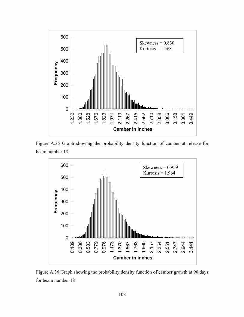
0

100

200

300

400

500

600

1.23

2

1.38

0

1.52

8

1.67

6

1.82

3

1.97

1

2.11

9

2.26

7

2.41

5

2.56

2

2.71

0

2.85

8

3.00

6

3.15

3

3.30

1

3.44

9

Camber in inches

Freq

uenc

y



beam number 18

0

100

200

300

400

500

600

0.18

9

0.38

6

0.58

3

0.77

9

0.97

6

1.17

3

1.37

0

1.56

7

1.76

3

Camber in in

Freq

uenc

y


for beam number 18

108


1.96

0

2.15

7

2.35

4

2.55

1

2.74

7

2.94

4

3.14

1

ches


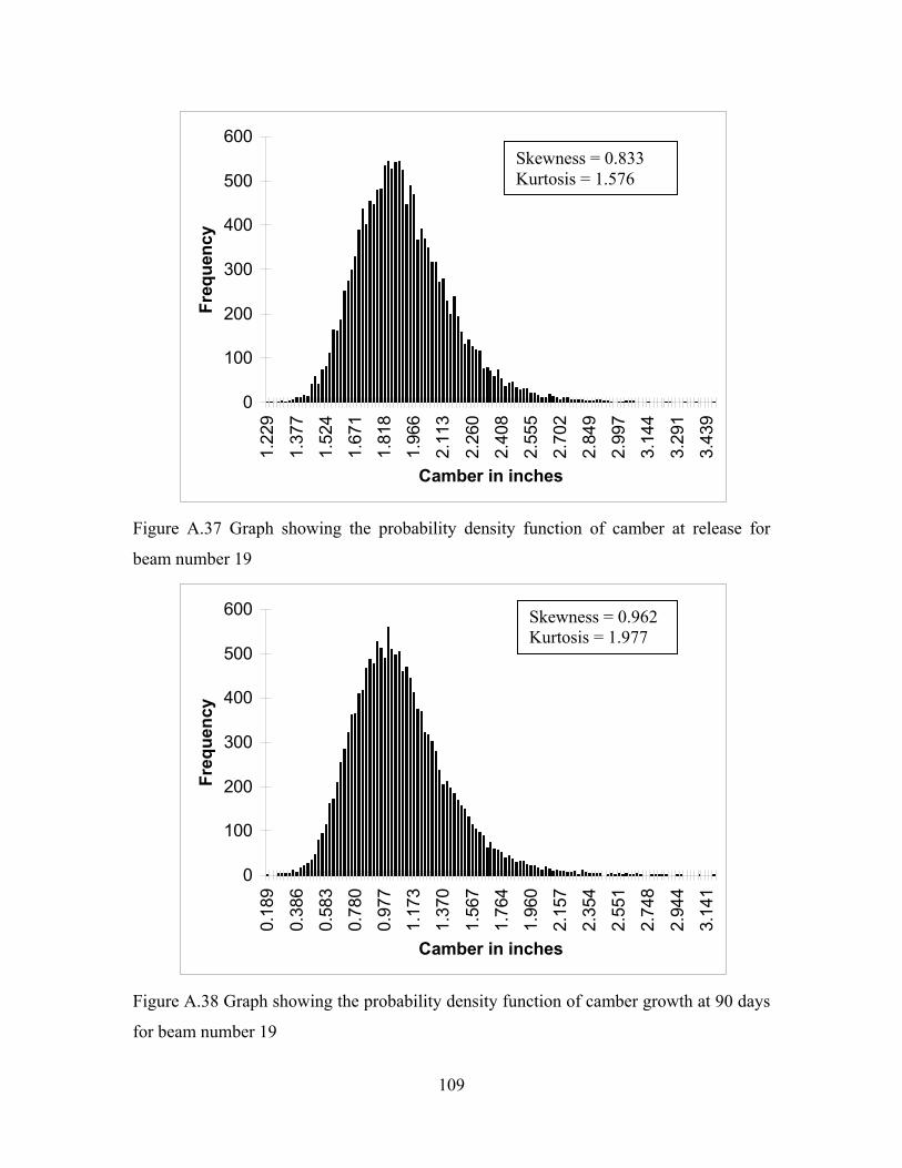
0

100

200

300

400

500

600

1.22

9

1.37

7

1.52

4

1.67

1

1.81

8

1.96

6

2.11

3

2.26

0

2.40

8

2.55

5

2.70

2

2.84

9

2.99

7

3.14

4

3.29

1

3.43

9

Camber in inches

Freq

uenc

y



beam number 19

0

100

200

300

400

500

600

0.18

9

0.38

6

0.58

3

0.78

0

0.97

7

1.17

3

1.37

0

1.56

7

1.76

4

1.96

0

2.15

7

2.35

4

2.55

1

2.74

8

2.94

4

3.14

1

Camber in inches

Freq

uenc

y



for beam number 19

109

0

100

200

300

400

500

600

1.17

0

1.31

4

1.45

8

1.60

2

1.74

6

1.89

0

2.03

4

2.17

8

2.32

3

2.46

7

2.61

1

2.75

5

2.89

9

3.04

3

3.18

7

3.33

1

Camber in inches

Freq

uenc

y



beam number 20

0

100

200

300

400

500

600

0.17

2

0.35

7

0.54

2

0.72

7

0.91

2

1.09

7

1.28

1

1.46

6

1.65

1

Camber in in

Freq

uenc

y


for beam number 20

110


1.83

6

2.02

1

2.20

6

2.39

1

2.57

6

2.76

1

2.94

6

ches


0

100

200

300

400

500

600

1.22

2

1.37

0

1.51

7

1.66

4

1.81

1

1.95

9

2.10

6

2.25

3

2.40

0

2.54

8

2.69

5

2.84

2

2.98

9

3.13

7

3.28

4

3.43

1

Camber in inches

Freq

uenc

y



beam number 21

0

100

200

300

400

500

600

0.18

6

0.38

1

0.57

5

0.77

0

0.96

5

1.16

0

1.35

5

1.54

9

1.74

4

1.93

9

2.13

4

2.32

8

2.52

3

2.71

8

2.91

3

3.10

8

Camber in inches

Freq

uenc

y



for beam number 21

111

Figure A.43 Dimension details of a PCBT sections used by VDOT. (VDOT)

112

Table A.1 Details for number of strands used in PCBT sections.

113

APPENDIX B

Appendix B contains the data sheets showing the strand pattern and the girder details of

the two samples used in the study done by Hinkle (2005).

114

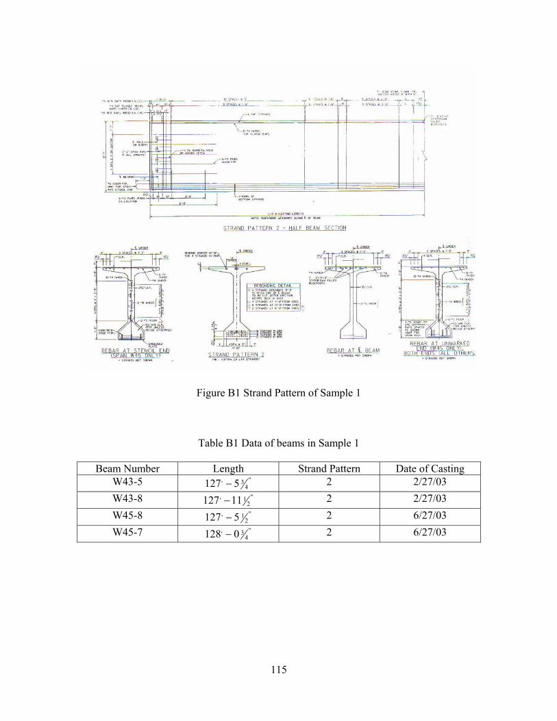
Figure B1 Strand Pattern of Sample 1

Table B1 Data of beams in Sample 1

Beam Number Length Strand Pattern Date of Casting W43-5 ", 3

4127 5− 2 2/27/03 W43-8 ", 1

2127 11− 2 2/27/03 W45-8 ", 1

2127 5− 2 6/27/03 W45-7 ", 3

4128 0− 2 6/27/03

115

Figure B2 Strand Pattern of Sample 2

Table B2 Data of beams in Sample 2

Beam Number Length Strand Pattern Date of Casting W23-4 ", 1

2136 6− 3 3/12/03 W24-3 ", 1

4136 9− 3 2/26/03 W23-3 ", 1

4136 9− 3 3/12/03 W27-7 ", 1

2136 9− 3 7/3/03

116

APPENDIX C

Appendix C contains sample design calculations for the post-tensioned anchorage zone

design for the unbonded monostrand anchorage. It also contains the procedure for

determining the correction achieved by using the unbonded monostrands. In addition, it

contains a data sheet showing the dimension details of the VSL type S6 monostrand

anchorage.

117

C.1.1 Assumptions

The following assumptions were made to perform these calculations:

1. Rectangular section behavior is assumed.

2. The critical section behind the group of anchorages is assumed at h/3 from the

first bearing surface of the anchorage.

3. The length of the local zone is assumed to be equal to the length of anchorage

plus twice the edge distance of anchorage.

4. Rate of dispersion of compressive stress is assumed as 1:2 from the edge of

bearing plate for e/b>3.

The size of type S6 anchorage is 4.13x2.95 inches.

C.1.2 Feasibility Check for Anchorage Arrangement in the PCBT Girder with No

Draped Strands

C.1.2.1 Vertical Bearing Plates

Referring to Figure 5.9 and using the Guyon’s method

'0.80jack ps sP A= f = 0.8x0.217x270 = 46.9 kips

Calculate the bursting force and stress around the two vertical anchorages in the middle.

From Equation 5.6

46.9 4.131 3.824 6.13burstT k⎛ ⎞= − =⎜ ⎟

⎝ ⎠ips

where

118

b is the bearing plate width and is equal to 4.13,

h is the member height and is equal to b plus twice the edge distance of 1 in. on each side,

P is the jacking force applied to one strand.

Calculate max ft using Equation 5.8

3.82max0.55 0.55 6.13 9.0

burstt

Tfhw

= =× ×

= 0.251 ksi

where, w is the member width calculated using assumptions 2 and 4.

The c/c distance of the middle two anchorages is 4 in.

Therefore w = 4+2.95+2.04(h/3) = 9.0 in.

Check this bursting stress against the allowable bursting stress

Allowable bearing stress is given by Equation C.1

' 4tallowable f f= ci (C.1)

where f’ci concrete strength at the time of stressing in psi.

The concrete strength chosen here is 5000 psi as this is the lowest concrete strength used

in the PCBT’s used by VDOT.

Therefore allowable ft = 0.283 ksi.

For vertical anchorages allowable ft is greater than max ft therefore it is ok.

C.1.2.2 Bearing Stresses Behind Vertical Anchorages

Bearing stress behind each anchorage is checked using Equations 5.4 and 5.5. The

method of checking the bearing stress is as follows: first the bearing stress under the first

vertical anchorage is checked and then the bearing stress under the adjacent vertical

anchorage is checked. Then the bearing stress under the two anchorages combined is

checked.

Using Equation 5.4, the allowable bearing stress under the bearing plate is:

36.1670.5 512.183cpif = × × =4.30ksi < 5.0ksi

119

where

f’ci=5 ksi, is the concrete strength at the time of stressing,

A=36.167, is the distribution area given as axay,

Ag = 12.183 is the gross bearing plate area given as bxby.

ax = bx + 2ex≤2bx

ay = by + 2ey≤2by

where bx, by are the dimensions of the bearing plate and ex, ey are the edge distances to

the bearing plates.

The limitation on the above equation is 14 4x

y

ee≤ ≤

The average bearing stress using Equation 5.3 is

46.94.13 2.95×

= 3.84 ksi < 4.30 ksi. Hence Ok

For the second bearing plate stress adjacent to the first one, the allowable bearing stress is

24.520.5 5 3.5412.183

× × = ksi.

As the allowable stress is less than the actual average bearing stress under the plate, we

need to check the combined bearing stress under the two anchorages.

The combined allowable average bearing stress is given as

8.95 6.130.5 5 3.752 12.183

×× × =

×ksi < 5.0 ksi

where ax = 8.95, is equal to the out to out edge distance of the two bearing plates plus the

edge distance of one inch on either side.

ay = 6.13 is the length of the bearing plate plus the edge distance of 1 in. on either side.

The dimensions for ax, ay are chosen in such a way that they lead to conservative design

values.

The average bearing stress under the two plates is

2 46.94.13 6.95

××

=3.26 ksi < 3.75 ksi

where, 6.95 is the out to out edge distance of the bearing plates in inches.

120

Therefore, the stress under the combined action of plates is ok and no confinement

reinforcement is required.

C.1.2.3 Horizontal Bearing Plates

Referring to Figure 5.9, the bursting stress for horizontal anchorage is

46.9 2.951 4.804 5burstT k⎛ ⎞= − =⎜ ⎟

⎝ ⎠ips

where

b is the bearing plate width equal to 2.95 in.,

h is the member height and is equal to b plus twice the edge distance of 1 inch on each

side,

P is the same as above.

The maximum bursting stress is

4.80max0.55 0.55 5 5.80

burstt

Tfhw

= =× ×

= 0.300 ksi

where, w is the member width calculated using assumptions 2 and 4,

Therefore w = 4.13+1.67(h/3) =9.0 in.

Checking this bursting stress against the allowable bursting stress gives

0.300 ksi > 0.283 ksi therefore the flange requires bursting reinforcement behind this

anchorage.

C.1.2.4 Bursting Reinforcement

Using 1.2 as the load factor and 0.85 as the resistance factor the required bursting

reinforcement is (Wollmann et al. 2000)

21.2 4.80 0.110.85 60sA in×

= =×

(C.2)

Therefore, provide #3 bars vertical tie behind each horizontal anchorage

121

C.1.2.5 Bearing Stress Behind Horizontal Anchorage

From Equation 5.4 the allowable bearing stress under the horizontal anchorage is

8.26 50.5 512.183

×× × = 4.60 ksi < 5.0 ksi Ok

where ax = 2x2.17 + 4.13 = 8.67 > 8.26 (2bx); ax = 8.26 in.

ay = 2x1 + 2.95 = 4.95 < 5.9 (2by); ay = 5 in.

The average bearing stress under the horizontal anchorage is

46.94.13 2.95×

= 3.84 ksi < 4.60 ksi Ok

C.1.2.6 Compressive Stress at the End of Local Zone

The length of the local zone for a conservative design is taken as the smaller dimension

of the anchorage plus twice the edge distance of one inch.

Therefore Llz = 2.95 + 2x1 = 4.95 in.

Using assumption 4 for rate of dispersion, the length at the end of the local zone for all

the four anchorages is given as 19.55 + 4.95 = 24.5 in.

The depth at the end of local zone is 5 inches i.e. the maximum depth available for

horizontal anchorages for a conservative design.

So the stress at the end of the local zone is

4 46.924.5 5×

× = 1.53 ksi < 2.5 ksi (0.5f’ci)

Therefore, it is feasible to provide four anchorages in the top flange of a PCBT, which

does not have any draped strands.

122

C.1.3 Feasibility Check for Anchorage Arrangement in PCBT Girder with Draped

Strands

Referring to Figure 5.10 and using a similar approach as used in Section C.1.2.3 for

horizontal bearing plates we would have to provide a #3 vertical tie behind each

anchorage.

C.1.3.1 Bearing Stress Behind Horizontal Anchorage

Using Equation 5.4 the allowable bearing stress under the horizontal anchorage is

8.26 50.5 512.183

×× × = 4.60 ksi < 5.0 ksi Ok

where ax = 2x2.17 + 4.13 = 8.67 > 8.26 (2bx); ax = 8.26 in.

ay = 2x1 + 2.95 = 4.95 < 5.9 (2by); ay = 5 in.


46.94.13 2.95×

= 3.84 ksi < 4 60 ksi Ok

For the second bearing plate adjacent to the first one the allowable bearing stress is

5.13 50.5 512.183

×× × = 3.84 ksi < 5.0 ksi Ok

where ax = 2x0.5 + 4.13 = 5.13 < 8.26 (2bx); ax = 5.13 in.

ay = 2x1 + 2.95 = 4.95 < 5.9 (2by); ay = 5 in.


2 46.98.76 2.95

××

= 3.63 ksi < 4.60 ksi Ok

where 8.76in., is the out to out edge distance of the horizontal bearing plates.

123

C.1.3.2 Compressive Stress at the End of Local Zone

The length of the local zone for conservative design is taken as the smaller dimension of

anchorage plus twice the edge distance of one inch.

Therefore Llz = 2.95 + 2x1 = 4.95 in.

Using assumption 4 for rate of dispersion, the length at the end of the local zone for all

the four anchorages is given as 23.00 + 4.95 = 27.95 in.

The depth at the end of local zone is 5 in. i.e. the maximum depth available for horizontal

anchorages for a conservative design value.

So the stress at the end of the local zone is

4 46.927.95 5×

×= 1.342 ksi < 2.5 ksi (0.5f’ci)

Therefore, it is feasible to provide four anchorages in the top flange of a PCBT, which

has draped strands.

C1.4 Camber Control Using Unbonded Monostrands

For controlling camber, the following steps were followed to determine the camber

controlled by four 0.6 in. monostrands.

1. Calculate the transformed section properties of the beam.

( 1)tr g pc psA A n A= + − (C.3)

( 1)g bg pc ps cgbtr

tr

A y n A yy

A+ −

= (C.4)

2( ) ( 1) (tr g g btr bg pc ps btr cg2)I I A y y n A y y= + − + − − (C.5)

where

Ag is the gross sectional area of the beam, in.2,

Aps is the total area of prestressing strands, in.2,

ybg is the distance of the center of gravity of the gross section of the beam from extreme

fiber of bottom flange, in.,

124

ycg is the distance of the center of gravity of the prestressing strands from extreme fiber

of bottom flange, in.,

Atr is the area of the equivalent transformed section of the beam, in.2,

ppc

c

En

E= (C.6)

npc is the modular ratio,

Ep is the modulus of elasticity of prestressing strands, ksi,

Ec is the modulus of elasticity of concrete at the time of stressing of steel, ksi,

ybtr is the distance of the center of gravity of the equivalent transformed section of the

beam from the extreme fiber of the bottom flange, in.,

Itr is the second moment of area of the equivalent transformed section, in.4.

2. Calculate the effective force in monostrands

_0.70monostrands pu ps monostrandsP f A= (C.7)

The above Equation calculates the effective force in monostrands after instantaneous

friction and seating losses.

3. Calculate the stresses at the extreme fibers of the beam

(monostrands monostrands btrtop

tr tr

P P e hfA I

)y−= + (C.8)

monostrands monostrands btrbot

tr tr

P PfA I

= −ey (C.9)

where

ftop is the stress at extreme top fiber of the beam,

e is the eccentricity of the post tensioned monostrands with respect to the center of

gravity of the equivalent transformed section,

h is the height of the section,

fbot is the stress at the extreme bottom fiber of the beam.

4. Calculate strains at the extreme fibers of the beam using the Hooke’s law

125

toptop

c

fE

ε = (C.10)

botbot

c

fE

ε = (C.11)

5. Calculate curvature of the transformed section

bot top

hε ε

φ−

= (C.12)

6. Calculate the curvature at various sections along the length of beam up to

midspan using the above steps and plot the curvature diagram.

7. Calculate the downward deflection using the moment area method.

126

Figure C.1 Data sheet showing the dimension details of type S6 anchorage used.

127

VITA

Vivek Sethi was born on May 30, 1980 in Madras, India. He completed his high school

from Ramjas School- Pusa Rd, New Delhi in 1997. He graduated with Bachelor of

Engineering in Civil Engineering from Punjab Engineering College, Chandigarh in 2001.

He worked for 3 years in Simplex Concrete Piles (I) Ltd. as Assistant Engineering (Civil)

on a large-scale infrastructure project. Vivek Sethi joined Virginia Tech for pursuing

Master of Science in Civil Engineering in August 2004.

128

UNBONDED MONOSTRANDS FOR CAMBER … · 2.5.3.1 NCHRP 496 Shrinkage Model..... 23 2.5.4 Prestressing...

Documents

Transcript of UNBONDED MONOSTRANDS FOR CAMBER … · 2.5.3.1 NCHRP 496 Shrinkage Model..... 23 2.5.4 Prestressing...